Applied Numerical Mathematics 106 (2016) 1–23

Contents lists available at ScienceDirect

Applied Numerical Mathematics

www.elsevier.com/locate/apnum

Sensitivity analysis for active control of the Helmholtz

equation

M. Hubenthal b, D. Onofrei a,∗a Department of Mathematics, University of Houston, Houston, TX 77004, United Statesb Institute for Mathematics and its Applications, University of Minnesota, Minneapolis, MN 55455, United States

a r t i c l e i n f o a b s t r a c t

Article history:Received 5 September 2015Received in revised form 12 March 2016Accepted 17 March 2016Available online 21 March 2016

Keywords:Active exterior cloakingHelmholtz equationIntegral equationsRegularization

In previous works we considered the Helmholtz equation with fixed frequency k outside a discrete set of resonant frequencies, where it is implied that, given a source region Da ⊂ R

d (d = 2,3) and u0, a solution of the homogeneous scalar Helmholtz equation in a set containing the control region Dc ⊂ R

d , there exists an infinite class of boundary data on ∂ Da so that the radiating solution to the corresponding exterior scalar Helmholtz problem in Rd \ Da will closely approximate u0 in Dc . Moreover, it will have vanishingly small values beyond a certain large enough “far-field” radius R .In this paper we study the minimal energy solution of the above problem (e.g. the solution obtained by using Tikhonov regularization with the Morozov discrepancy principle) and perform a detailed sensitivity analysis. In this regard we discuss the stability of the minimal energy solution with respect to measurement errors as well as the feasibility of the active scheme (power budget and accuracy) depending on: the mutual distances between the antenna, control region and far field radius R; value of the regularization parameter; frequency; location of the source.

© 2016 IMACS. Published by Elsevier B.V. All rights reserved.

1. Introduction

The current literature has significantly addressed the idea of active manipulation of vector and scalar fields in desired regions of space.

In fact the active (partial) nulling of fields in the low-frequency acoustics was first studied in [21] (feed-forward control of sound) and in [28] (feedback control of sound). The reviews [33,15,19,20,32,9,31,7] and references therein discuss the active sound control problem for arbitrary finite frequency.

For cloaking applications, the strategy proposed in [26] employs a continuous active layer on the boundary of the control region while the scheme discussed in [11–14,10] (see also [37]), uses a discrete number of active sources located in the exterior of the control region to manipulate the fields. These field manipulation problems may be thought of as a prelude to the recommended line of research proposed here. In these works, manipulation of electrostatic fields has been treated as well as time varying scalar fields in two and three dimensions by using integral representation theorems. These results were further extended in [27], where a detailed sensitivity analysis is presented.

* Corresponding author.E-mail addresses: huben003@umn.edu (M. Hubenthal), onofrei@math.uh.edu (D. Onofrei).

http://dx.doi.org/10.1016/j.apnum.2016.03.0030168-9274/© 2016 IMACS. Published by Elsevier B.V. All rights reserved.

2 M. Hubenthal, D. Onofrei / Applied Numerical Mathematics 106 (2016) 1–23

In a parallel development in [34,35] the authors make use of the equivalence principle and show how a dipole array can cancel the known electromagnetic scattered field from a cylinder. Further experimental results on active cloaking are presented in [22] for the quasistatic regime and in [6] for the finite frequency regime.

Yet another approach for active cloaking is the use of essentially non-radiating sources. The works [24,23] and [25]studied the structure of such sources and in [5,4] the author considered their applications for the active cloaking.

In [2] an alternative active scattering cancellation strategy is proposed where it is shown that suitably designed active meta-surfaces (e.g., active smart electrical circuits) can in principle be tuned to suppress the scattering from known incident fields. These results are supported by simulation and in [36] experimental proof was obtained for a cylindrical scatterer of 2.2-wavelengths in length and 0.31-wavelengths in cross section. In all the above works foreknowledge of the fields to be reduced was available.

The active manipulation of quasistatic fields by using one source was studied with the help of boundary layer potentials in [29]. Recently in [30] we extended the results presented in [29] to the active control problem for the exterior scalar Helmholtz equation. In particular, we characterized an infinite class of boundary functions on the source boundary ∂ Daso that we achieve the desired manipulation effects in several mutually disjoint exterior regions. The method is novel in the sense that instead of using microstructures, exterior active sources modeled with the help of the above boundary controls are employed for the desired control effects. Such exterior active sources can represent velocity potential, pressure or currents depending on the regime of interest.

In the current paper we propose a sensitivity and feasibility study for the minimal norm solution of the active manipu-lation problem considered in [29,30]: one antenna Da approximating a given field in a prescribed near field control region Dc with very little radiation on ∂ B R(0), with R � 1 (see Fig. 1). We make use of the results in [30] and present a detailed sensitivity and feasibility study for the minimal norm solution of the problem. As we will explain in Section 2 this problem may be relevant to protection from unwanted interrogation as well as for the question of near field synthesis with small far field radiation.

The paper is organized as follows: In Section 2 we present the physical motivation behind our study. In Section 3we recall the general result obtained in [30] in the context of exterior active cloaking. Section 4 we present an L2

conditional stability result for the minimal norm solution with respect to measurement errors of the incoming field. In Section 5 we present the numerical details of the Tikhonov regularization algorithm with the Morozov discrepancy prin-ciple for the computation of the minimal norm solution of the exterior active cloaking problem in two dimensions. We will numerically observe the fact that the scheme requires large antenna powers in the far field and we will provide nu-merical support for our theoretical stability results. An important part of this section will be focused on the sensitivity analysis, where we will study: the dependence of the control results as a function of mutual distances between the an-tenna, control region and far field region; and the broadband character of our scheme in the near field region. Finally, in Section 6 we highlight the main results of the paper and discuss current and future challenges and extensions of our research.

2. Motivation and main results

The motivation behind our work is the desire to create stable, low budget schemes, for the approximation of desired fields in the exterior of controlled active sources with possible applications in antenna synthesis, inverse source problems, and electromagnetic or acoustic cloaking/shielding.

Our analysis focuses on a the following situation:

Problem. A single active antenna, Da , approximates a desired pattern in its near field region, Dc , with very little spillover in the far field (e.g. beyond a certain fixed radius R).

The geometry of the problem is sketched in Fig. 1. In Proposition 4.1 and Corollary 4.1 we prove, under suitable source type conditions, the stability of the minimal energy solution (the Morozov solution) of the above problem. In Section 5 we also provide a sensitivity numerical analysis of the minimal energy solution (e.g., its stability, power budget and accuracy) with respect to various parameters: distance between antenna Da and control region Dc , wave number k, noise level ε , far field boundary R . The numerical sensitivity analysis performed in Section 5 suggest that the scheme proposed by us has a broadband character and is feasible (good accuracy with good power budget) only in a thin sub region in the near field of the sources but possible for a wide enough angular span.

Our result proposes a stable scheme for the synthesis of active sources with controllable near fields and very weak far fields and, besides their possible applicability in near field synthesis applications, this type of sources are theoreti-cally very important in the analysis of the inverse source problems since they are near the kernel of the far field operator and thus are the main cause of instabilities. Their understanding will guide us to a proper penalization of the cost func-tional to avoid such instabilities. A separate publication with the 3D analysis is in preparation and will be communicated soon.

The presented results imply that one can control a thin but angularly wide near field region of a small active weak radiator and this fact implies the possibility to build a suitable array of such elements with the property that they will cancel an incoming field with very little radiation in the far field. Thus, paired with an appropriate feedback control loop,

M. Hubenthal, D. Onofrei / Applied Numerical Mathematics 106 (2016) 1–23 3

Fig. 1. An antenna defined by ∂Da with a control region Dc and far field region B R (0).

we believe that such an array could be mounted in a thin electromagnetic transparent skin around a given scatterer (the array being a small distance away from the scatterer) and protect it from unwanted interrogation by canceling the incident field in the region between the array and the scatterer.

The same question in the acoustic regime is currently studied by our group and will be reported in a forthcoming publication.

3. Background

In this section we will recall the main result regarding the active exterior control problem for the Helmholtz equation obtained in [30]. We will focus only on the case where one active external source (antenna) Da protects a control region Dc from an interrogating far field and maintains an overall small signature beyond a disk of large enough radius R .

The general setup for this question will be as follows. Let B R ⊂ Rd be the ball of radius R > 0. We assume 0 ∈ Da ⊂ B R

is the region inside a single antenna with sufficiently smooth boundary ∂ Da . We also let Dc � B R be the control region, which is assumed to satisfy Dc ∩ Da = ∅ (see Fig. 1). The numerical simulations in the current work are performed for the two dimensional case but the methods are adaptable to the three dimensional setting as well. Consider the function space

� = L2(∂ Dc) × L2(∂ B R),

endowed with the scalar product

(φ,ψ)� =∫

∂ Dc

φ1(y)ψ1(y)dSy +∫

∂ B R

φ2(y)ψ2(y)dSy, (3.1)

which is a Hilbert space. For the remainder of the paper we will assume that every L2 space of complex valued functions will be endowed with the usual inner product. As in [30] consider K : L2(∂ Da) → �, the double layer potential operator restricted to ∂ Dc and ∂ B R , respectively, defined by

Kφ(x, z) = (K1φ(x), K2φ(z)), φ ∈ L2(∂ Da), (3.2)

where

K1 : L2(∂ Da) → L2(∂ Dc), K1φ(x) =∫

∂ Da

φ(y)∂�(x,y)

∂νydsy, for x ∈ ∂ Dc,

K2 : L2(∂ Da) → L2(∂ B R), K2φ(z) =∫

∂ Da

φ(y)∂�(z,y)

∂νydsy, for z ∈ ∂ B R(0). (3.3)

Here �(x, y) represents the fundamental solution of the relevant Helmholtz operator, i.e.,

�(x,y) =

⎧⎪⎪⎨⎪⎪⎩eik|x−y|

4π |x − y| , for d = 3

i4 H (1)

0 (k|x − y|), for d = 2

(3.4)

with H (1)0 = J0 + iY0 representing the Hankel function of first type. Note that in (3.3) the integrals are to be understood as

singular integrals defined through an operator extension from C(∂ Da). We will also consider k such that

4 M. Hubenthal, D. Onofrei / Applied Numerical Mathematics 106 (2016) 1–23

1) − k2 is not a Neumann eigenvalue for the Laplace operator in Da or B R(0),

2) − k2 is not a Dirichlet eigenvalue for the Laplace operator in Dc. (3.5)

As in [30] we introduce the adjoint operator K ∗ : � → L2(∂ Da), which can be shown to satisfy

K ∗ψ(x) =∫

∂ Dc

ψ1(y)∂�(y,x)

∂νxdSy +

∫∂ B R

ψ2(y)∂�(y,x)

∂νxdSy, x ∈ ∂ Da. (3.6)

This paper proposes a sensitivity study for the following problem: Let V � Dc and R ′ > R . For a fixed wave number k > 0 and fixed 0 < μ 1, find a function h ∈ C(∂ Da) such that there exists u ∈ C2(Rn \ Da) ∩ C1(Rn \ Da) solving⎧⎪⎨⎪⎩

( + k2)u(x) = 0 x ∈Rn \ Da

u = h on ∂ Da

‖u − f1‖C(V ) = O(μ) and ‖u‖C(Rn\B R′ (0)) = O(μ),

(3.7)

where f1 is a solution of the Helmholtz equation in a neighborhood of the control region Dc . In fact, by using the operator K and regularity arguments it is shown in [30] that a class of solutions for problem (3.7) can be obtained by considering the following problem: for a fixed wave number k > 0 satisfying conditions (3.5), a given function f = ( f1, 0) ∈ � and μ > 0, find a density function φ ∈ C(∂ Da) such that

‖Kφ − f ‖� ≤ μ. (3.8)

Problem (3.8) is in fact a Fredholm integral equation of the first kind, and it was studied in a very general setting in [30]. There the authors proved that the bounded and compact operator K is also one-to-one and has a dense (but not closed) range, thus proving the existence of a class of solutions for (3.8) (and thus for (3.7)). However, the fact that Kis compact and that its range is not closed also implies that problem (3.8) is ill-posed. By using regularization, one can approximate a solution to problem (3.8) with an arbitrary level of accuracy μ 1. There are several methods known in the literature, but we will use in this paper the Tikhonov regularization method [8,1]. This method, when applied to the operator K : L2(∂ Da) → �, proposes a solution φα ∈ C(∂ Da) of the form

φα = (α I + K ∗K )−1 K ∗ f , for 0 < α 1, (3.9)

where α is a suitably chosen regularization parameter.It is known that ‖Kφα − f ‖� → 0 as α → 0, (see [17], Theorem 2.16), but the optimal choice of α is an essential step

in designing a feasible method (e.g., finding a minimal norm solution), and there are various modalities to do this. In this paper we will use the Morozov discrepancy principle associated to the following weighted residual:

E(φ,h) = 1

‖h1‖2L2(∂ Dc)

‖K1φ − h1‖2L2(∂ Dc)

+ 1

2π R‖K2φ‖2

L2(∂ B R ), (3.10)

for every given h = (h1, 0) ∈ �. The reasoning behind using the weighted residual discrepancy functional defined at 3.10 is as follows. Due to the asymptotic behavior of ∂�(x, y)

∂νy=O(|x − y|−1/2) as |x − y| → ∞, we have that given a fixed density φ,

‖Kφ‖L2(∂ B R ) = O(1) as R → ∞. In other words, using the space L2(∂ B R) with the standard surface measure is not really suited to the decay properties of double layer potential solutions, because the decay of the normal derivative ∂ν� is too weak. Similarly, we use the relative norm

‖K1φ − h1‖L2(∂ Dc)

‖h1‖L2(∂ Dc)

(3.11)

on ∂ Dc because this is a useful quantity for determining how good the control is, regardless of the norm of h1. Thus our procedure for finding an approximate solution for problem (3.8) is to first make use of the Tikhonov regularization for the operator K : L2(∂ Da) → � as described in (3.9) to obtain φα and then apply the Morozov’s discrepancy principle for the choice of α ([18]), i.e. such that

E(φα, f ) = δ2, (3.12)

with δ2 ≤ μ2 min

{1

2‖ f1‖2L2(∂ Dc)

,1

4π R

}.

In what follows, we will account for noise and measurement errors and will consider (3.12) with f = ( f1, 0) ∈ � replaced by fε = ( fε,1, fε,2) ∈ �, given by

fε = ( f1 + εs, 0) ∈ �, (3.13)

M. Hubenthal, D. Onofrei / Applied Numerical Mathematics 106 (2016) 1–23 5

where s ∈ L2(∂ Dc) is a random perturbation with ‖s‖L2(∂ Dc)≤ 2‖ f1‖L2(∂ Dc)

and f1 is a solution of the Helmholtz equation in a neighborhood of the control region Dc . We mention that in the numerical experiments of Section 5, f1 denotes the k frequency component of the far field of a far field observer. Note that this assumption about the interrogating signal ensures that f1 is a solution of the Helmholtz equation in B R . In the noisy case (i.e. when f is replaced by fε ) equation (3.12) becomes

E(φα, fε) = δ2, (3.14)

where φα = (α I + K ∗K )−1 K ∗ fε is the Tikhonov regularization solution. From the definition of E and classical results, [17,18], it follows that (3.14) admits at least a solution α. Moreover, as we will discuss in Section 4, motivated by numerical evidence, we formulate the hypothesis that there exists ε0 > 0 such that for each ε ∈ (0, ε0), problem (3.14) has a unique solution α(ε) which uniquely defines a differentiable function ε � α(ε). We will study the minimal norm solution uniquely determined by (3.14), discuss its stability for given noisy data in � and, in the case of data corresponding to a point source, analyze its sensitivity with respect to parameters such as: mutual distances between Da , Dc and B R(0); wave number k; and the location of the point source.

4. Stability estimate for the Tikhonov regularization

In this section we present analytical and numerical arguments which indicate the stability of the minimum norm solution φα with respect to noise level ε for a given fixed discrepancy level δ. Next, we present below Lemma 4.1 which will provide bounds for ‖ f1‖L2(∂ DC ) and α in terms of the operatorial norm of K ∗

1 .

Lemma 4.1. Let 0 < δ < 1√2

and z = (z1, 0) ∈ � with z1 �= 0. Consider vα = (α I + K ∗K )−1 K ∗z ∈ C(∂ Da), with α such that E(vα, z) ≤ δ2 . Then we have

‖z1‖L2(∂ Dc)≤ 4‖K ∗

1‖O‖vα‖L2(∂ Da), (4.1)

α ≤ 4δ‖K ∗1‖2

O, (4.2)

where K ∗1 is the adjoint operator for K1 defined by (3.3) and ‖ · ‖O denotes the operatorial norm.

Proof. We will start with the proof of (4.1). Note that since E(vα, z) ≤ δ2, we have

‖K1 vα − z1‖2L2(∂ Dc)

≤ δ2‖z1‖2L2(∂ Dc)

. (4.3)

From (4.3) we obtain

‖K1 vα‖2L2(∂ Dc)

− 2 Re(K1 vα, z1)L2(∂ Dc)+ ‖z1‖2

L2(∂ Dc)≤ δ2‖z1‖2

L2(∂ Dc), (4.4)

and this implies

‖z1‖2L2(∂ Dc)

(1 − δ2) ≤ 2 Re(vα, K ∗1 z1)L2(∂ Da)

≤ 2‖vα‖L2(∂ Da)‖K ∗

1 z1‖L2(∂ Da). (4.5)

Then (4.5) gives

‖vα‖L2(∂ Da)≥

‖z1‖2L2(∂ Dc)

(1 − δ2)

2‖K ∗1 z1‖L2(∂ Da)

=(

1 − δ2

2

)( ‖z1‖L2(∂ Dc)

‖K ∗1 z1‖L2(∂ Da)

)‖z1‖L2(∂ Dc)

≥ 1 − δ2

2

(‖z1‖L2(∂ Dc)

‖K ∗1‖O

)≥ ‖z1‖L2(∂ Dc)

4‖K ∗1‖O . (4.6)

Next we proceed towards proving (4.2). From the definition of vα we have

αvα + K ∗K vα = K ∗z = K ∗1 z1,

αvα + K ∗2 K2 vα = K ∗

1 (z1 − K1 vα). (4.7)

Here we have used from (3.3) and (3.6) that

K ∗ψ = K ∗1ψ1 + K ∗

2ψ2, for all ψ ∈ �,

K ∗K w = K ∗K1 w + K ∗K2 w, for all w ∈ L2(∂ Da). (4.8)

1 2

6 M. Hubenthal, D. Onofrei / Applied Numerical Mathematics 106 (2016) 1–23

Multiplying (4.7) with vα in the sense of the usual scalar product in L2(∂ Da), we obtain

α‖vα‖2L2(∂ Da)

+ ‖K2 vα‖2L2(∂ Da)

= (K ∗1 (z1 − K1 vα), vα)L2(∂ Da)

. (4.9)

Using (4.3), (4.6) and (4.8) in (4.9) we then have

α‖vα‖L2(∂ Da)≤ δ‖K ∗

1‖O‖z1‖L2(∂ Dc)=⇒ α ≤ 4δ‖K ∗

1‖2O. �

Consider the function g : (0, ∞) × (0, ∞) → (0, ∞) defined by

g(α, ε) = E(φα, fε), (4.10)

where fε ∈ � was introduced in (3.13), and φα is the Tikhonov regularization solution introduced in (3.14). With this notation, (3.14) can be rewritten as

g(α, ε) = δ2, (4.11)

where δ is the desired fixed discrepancy level. By using classical results (e.g., [17,18]) it can be observed that for every ε , (4.11) admits at least one solution in (0, ∞) and that g defined by (4.10) is differentiable with respect to positive α and ε , respectively. In fact, it follows from classical arguments that a maximum value of α for a given ε exists. This solution of (4.11) corresponds to the L2 minimal energy solution and we will further refer to it as the Morozov solution.

For the remainder of the paper, unless otherwise specified, C will denote a generic constant which depends only on the operator K , dc = diam(Dc) and d = dist(∂ Dc, ∂ Da). The next Proposition states a central stability result concerning the Morozov solution of (4.11). We have,

Proposition 4.1. Let 0 < δ be as above, and fε and f1 as defined in (3.13). For every ε ≥ 0 consider φαε = (αε I + K ∗K )−1 K ∗ fε ∈C(∂ Da) with αε = α(ε) the Morozov solution of (4.11). Then we have,

‖φαε − φα0‖L2(∂ Da)

‖φαε ‖L2(∂ Da)

≤

∣∣∣∣αε

α0− 1

∣∣∣∣+√∣∣∣∣αε

α0− 1

∣∣∣∣2 + 64ε (2δ + Cδε + Cε)

α0‖K ∗

1‖2O

2. (4.12)

Proof. Fix ε > 0 and let f = fε for ε = 0. Let us recall that α(ε) is uniquely implicitly defined by the equation E((αε I +K ∗K )−1 K ∗ fε, fε) = δ2 and by Lemma 4.2 it will be differentiable in some interval (0, ε0) for all wavenumbers k. Next consider

αεφαε + K ∗Kφαε = K ∗ fε,

α0φα0 + K ∗Kφα0 = K ∗ f ,

where α0 = α(0), f0 = ( f1, 0) (as in (3.13)) and φα0 = (α0 I + K ∗K )−1 K ∗ f0. Subtracting, we obtain

α0φα0 − αεφαε + K ∗K (φα0 − φαε ) = K ∗( f − fε),

α0(φα0 − φαε ) + (α0 − αε)φαε + K ∗K (φα0 − φαε ) = K ∗( f − fε). (4.13)

Integrating both sides of (4.13) against φα0 − φαε yields

α0‖φα0 − φαε ‖2L2(∂ Da)

+ (α0 − αε)(φαε , φα0 − φαε )L2(∂ Da)+ ‖K (φα0 − φαε )‖2

�

= (K (φα0 − φαε ), f − fε)� = (K1(φα0 − φαε ), f1 − fε,1)L2(∂ Dc), (4.14)

where, we have used (3.3) and the fact that f2 = fε,2 = 0 in the last equality above. Thus,

α0‖φα0 − φαε ‖2L2(∂ Da)

≤ |α0 − αε |‖φαε ‖L2(∂ Da)‖φα0 − φαε ‖L2(∂ Da)

+ ‖ f1 − fε,1‖L2(∂ Dc)‖K1(φα0 − φαε )‖L2(∂ Dc)

(4.15)

Observe that

‖K1(φα0 − φαε )‖L2(∂ Dc)≤ ‖K1φα0 − f1‖L2(∂ Dc)

+ ‖K1φαε − fε,1‖L2(∂ Dc)+ ‖ f1 − fε,1‖L2(∂ Dc)

≤ δ‖ f1‖L2(∂ Dc)+ δ‖ fε,1‖L2(∂ Dc)

+ Cε‖ f1‖L2(∂ Dc)

= (2δ + Cδε + Cε)‖ f1‖L2(∂ Dc), (4.16)

where fε,1 = f1 + εs with ‖s‖L2(∂ Dc)≤ C‖ f1‖L2(∂ Dc)

, and we have used the definition of φαε and (3.10) in the inequalities above. Using (4.16) in (4.15) we obtain

M. Hubenthal, D. Onofrei / Applied Numerical Mathematics 106 (2016) 1–23 7

Fig. 2. Plot of F (α) = E(φα, fε ) − δ2 for ε = 0.005 and α in a range where one can see its non-monotonic behavior below a particular threshold.

α0‖φα0 − φαε ‖2L2(∂ Da)

≤ |α0 − αε |‖φαε ‖L2(∂ Da)‖φα0 − φαε ‖L2(∂ Da)

+ ε (2δ + Cδε + Cε)‖ f1‖2L2(∂ Dc)

. (4.17)

If we define A := ‖φαε −φα0 ‖L2(∂ Da)

‖φαε ‖L2(∂ Da), inequality (4.17) implies that

α0 A2 ≤ |α0 − αε |A +ε (2δ + Cδε + Cε)‖ f1‖2

L2(∂ Dc)

‖φαε ‖2L2(∂ Da)

≤ |α0 − αε |A + 16ε (2δ + Cδε + Cε)‖K ∗1‖2

O, (4.18)

where we have used (4.1) of Lemma 4.1 in the last inequality above. Next, consider

h(A) := A2 −∣∣∣∣αε

α0− 1

∣∣∣∣ A − 16‖K ∗1‖2

Oε (2δ + Cδε + Cε)

α0.

Then, from (4.18) we have h(A) ≤ 0 and this implies that

A ≤

∣∣∣∣αε

α0− 1

∣∣∣∣+√∣∣∣∣αε

α0− 1

∣∣∣∣2 + 64‖K ∗1‖2

Oε (2δ + Cδε + Cε)

α0

2which completes the proof. �

Next, before presenting the main stability result of this section, we must understand under what conditions equation (4.11) admits a unique solution α(ε) with the property that the resulting function ε � α(ε) is differentiable.

We will first discuss the monotonic character of g as this will be essential in establishing the differentiability of α(ε). We first note that, as suggested by the numerics, g is not in general globally monotonic with respect to α as can be seen in Fig. 2, which considers an antenna of radius a = 0.01, region of control characterized in polar coordinates by r1 = 0.011, r2 = 0.015, θ ∈ [3π/4, 5π/4], wave number k = 10, fε given by (3.13) with f1 = 1

4 H (1)0 (k|x − x0|) with x0 = [10000, 0]T ,

and noise level ε = 0.005.On the other hand, for the same geometry and functional settings as in Fig. 2, we observe in Fig. 3 that for each ε

small enough, e.g. ε < 0.015, g(α, ε) = E(φα, fε) is strictly increasing with respect to α when α ∈ (10−4, 1). Moreover, for every ε < 0.015 the Morozov solution α(ε) is the unique solution of (4.11) in (10−4, 1). In other words, for this particular example we have that ∂

∂α g(α, ε) �= 0 in α = αε for ε < 0.015 and this together with the uniqueness and the implicit function theorem implies the differentiability of αε for ε < 0.015!

In fact, numerical results suggest that this conclusion is true for a broadband spectrum of k values. Indeed, let us consider the same geometry and functional settings as in Fig. 2, Fig. 3 with k ∈ [1, 100] and ε = 0.005. Table 1 summarizes the values

8 M. Hubenthal, D. Onofrei / Applied Numerical Mathematics 106 (2016) 1–23

Fig. 3. Plot of g(α, ε) = E(φα, fε ) and ∂∂α g(α, ε) with respect to α, ε together with the unique largest value α(ε) such that E(φαε , fε ) = δ2, where δ = 0.02

is fixed.

Table 1Table of values −pk such that g(α, ε) is increasing with respect to α for α ≥ 10−pk . ε is fixed at 0.005 in this case.

k −pk Morozov α

1.0 −5.74057337341 0.0021397

6.0 −5.15371857022 0.0022445

11.0 −4.61487654411 0.0027985

16.0 −4.43348001737 0.0037643

21.0 −7.22374205154 0.0052228

26.0 −6.73292218326 0.0072707

31.0 −6.41280555768 0.0098052

36.0 −6.18339417827 0.012607

41.0 −5.97530913764 0.015782

46.0 −5.78858575492 0.01971

k −pk Morozov α

51.0 −5.63387601498 0.023987

56.0 −5.5538513243 0.028226

61.0 −5.58052339557 0.032734

66.0 −7.93866063316 0.038053

71.0 −7.78393971408 0.043891

76.0 −7.60786606025 0.048884

81.0 −7.41580451387 0.05425

86.0 −7.2077344143 0.060871

91.0 −7.00500135956 0.066982

96.0 −6.90364624001 0.07278

of pk > 0 for which g(α, ε) is locally strictly monotonic with respect to α in an interval (10−pk , 1), as well as the value of the Morozov solution α(ε, k) for each k. We can see from Table 1 and Fig. 4 that α(ε, k) ∈ (10−pk , 1) and that dueto the monotonicity of g , α(ε, k) it is the unique solution of (4.11) in (10−pk , 1). This also suggests that ∂

∂α g(α, ε) �= 0in α = α(ε, k) for small enough ε , which again, together with the uniqueness and implicit function theorem, implies the differentiability of α(ε, k) for small enough ε!

For simplicity of notation, in what follows we will write sometimes α instead of αε = α(ε) and we will use α′ and f ′ε,i

to denote dαdε and dfε,i

dε respectively. Motivated by the above numerics, we formulate the following more general hypothesis:

Hypothesis 1. Assume the same geometrical setup as in Section 3 and let fε , f1 be as in (3.13). Then there exists p0 > 0and ε0 > 0 such that ∂

∂α g(α, ε) �= 0 in (10−p0 , 1) × (0, ε0) for all wave numbers k, and the Morozov solution α(ε) is the unique solution of (4.11) in (10−p0 , 1).

For example, as discussed above, for fε , f1 as in (3.13) with s = ν̂‖ f1‖L2(∂ Dc)where ̂ν ∈ L2(∂ Dc) is a random perturbation

with ‖̂ν‖L2(∂ Dc)= 1, and for the same geometry and data as in Fig. 2 and Fig. 3, we have that Hypothesis 1 is satisfied for

p0 = 10−4 and ε small enough for all k = 1,100. As a consequence of uniqueness and implicit function theorem we have that whenever Hypothesis 1 is satisfied, the definition of α(ε) and the implicit function theorem imply:

M. Hubenthal, D. Onofrei / Applied Numerical Mathematics 106 (2016) 1–23 9

Fig. 4. Threshold value pk for which F (α) is increasing when α > 10−pk . Also shows the value of α for which F (α) = δ2 with the same setting as in Fig. 3, where δ = 0.02 and the noise level ε = 0.005.

Lemma 4.2. There exists ε0 > 0 such that for every ε ∈ (0, ε0), the function α : (0, ε0) → (0, ∞), where for each ε ∈ (0, ε0), α(ε)

represents the Morozov solution of (4.11), will be differentiable for all wave numbers k.

The next Lemma is a technical result needed in the stability estimate obtained in Corollary 4.1.

Lemma 4.3. Let f1 be a solution of the Helmholtz equation in a neighborhood of Dc satisfying the following source type condition:∥∥∥∥∥K1ψ0 − f1

‖ f1‖L2(∂ Dc)

∥∥∥∥∥L2(∂ Dc)

≤ Cδ for some ψ0 ∈ L2(∂ Da) with ‖ψ0‖L2(∂ Da)≤ Cδ. (4.19)

Assume R (radius of B R(0)) is such that,

‖ f1‖L2(∂ Dc)≤ √

π R. (4.20)

Consider sε = f1 + ε2 ν̂‖ f1‖L2(∂ Dc)

where ̂ν ∈ L2(∂ Dc) is a random perturbation with ‖̂ν‖ ≤ 1. Assume the same functional framework as in Proposition 4.1 and that Hypothesis 1 holds true in the case when fε is given by

fε = ( fε,1, fε,2) = ( f1 + εsε, 0). (4.21)

Then, there exists ε0 > 0 such that the Morozov solution of equation (4.11) α = α(ε) satisfies

α|α′| ≤ Cδ2

√α

, for all ε < ε0. (4.22)

Proof. Define the weights

w1 := 1

‖ fε,1‖2L2(∂ Dc)

w2 := 1

2π R

and denote Tα := (K ∗K + α I)−1, Rα := Tα K ∗ . Then using the Einstein summation convention, we may write

E(φα, fε) = wi‖Kiφα − fε,i‖2L2(W i)

= wi (Kiφα − fε,i, Kiφα − fε,i)

L2(W i),

where W1 = ∂ Dc , W2 = ∂ B R . Next, as in Lemma 4.2, we observe that Hypothesis 1 together with the implicit function theorem imply the uniqueness and differentiability of α(ε), on the interval ε ∈ (0, ε0) for some ε0 > 0, where α(ε) is uniquely and implicitly defined by the equation E((αε I + K ∗K )−1 K ∗ fε, fε) = δ2. Differentiating the equation E((αε I +K ∗K )−1 K ∗ fε, fε) = δ2 with respect to ε and noting that δ is fixed, we obtain

10 M. Hubenthal, D. Onofrei / Applied Numerical Mathematics 106 (2016) 1–23

0 = ∂ε E(φα, fε) = 2wi Re(

Kiφ′α − f ′

ε,i, Kiφα − fε,i)

L2(W i)

− 2(w1)2 Re(

f ′ε,1, fε,1

)L2(∂ Dc)

‖K1φα − fε,1‖2L2(∂ Dc)

. (4.23)

Next, from (K ∗K + α I)φα = K ∗ fε we observe that

φ′α = Rα f ′

ε − α′Tαφα. (4.24)

Thus, we may write

Kiφ′α − f ′

ε,i = −α′Ki Tαφα + Ki Rα f ′ε − f ′

ε,i . (4.25)

By using (4.25) and (4.24) we obtain that

2(

Kiφ′α − f ′

ε,i, Kiφα

)L2(W i)

= −2α′ (Tαφα, K ∗i Kiφα

)L2(∂ Da)

+ 2(

Ki Rα f ′ε − f ′

ε,i, Kiφα

)L2(W i)

, (4.26)

and

−2(

fε,i, Kiφ′α − f ′

ε,i

)L2(W i)

= 2α′ ( fε,i, Ki Tαφα

)L2(W i)

− 2(

fε,i, Ki Rα f ′ε − f ′

ε,i

)L2(W i)

= 2α′ (K ∗i fε,i, Tαφα

)L2(∂ Da)

− 2(

fε,i, Ki Rα f ′ε − f ′

ε,i

)L2(W i)

. (4.27)

Let P , Q be defined by

P = 2wi[(

Kiφα − fε,i, Ki Rα f ′ε − f ′

ε,i

)L2(W i)

+ α′ (K ∗i fε,i − K ∗

i Kiφα, Tαφα

)L2(∂ Da)

](4.28)

Q = 2(w1)2 ( f ′ε,1, fε,1

)L2(∂ Dc)

‖K1φα − fε,1‖2. (4.29)

Then from (4.26), (4.27) used in (4.23) we obtain

0 = ∂ε E(φα, fε) = Re(P ) − Re(Q ). (4.30)

We focus first on P introduced in (4.28). In this regard, let us define

Li := (Kiφα − fε,i, Ki Rα f ′

ε − f ′ε,i

)L2(W i)

. (4.31)

Observe that (4.21) implies

f ′ε = ( f ′

ε,1, f ′ε,2) = ( f1 + εν̂‖ f1‖L2(∂ Dc)

,0). (4.32)

First note that by using classical arguments based on the singular value decomposition for K : L2(∂ Da) → �, one can adapt the results in [17] (Theorem 2.7) and obtain,

‖KRα K z − K z‖� ≤ C√

α‖z‖L2(∂ Da), for every z ∈ L2(∂ Da). (4.33)

Let f =(

f1

‖ f1‖L2(∂ Dc)

,0

)and v = f ′

ε

‖ f1‖L2(∂ Dc)

− f . By using the definition of E and �, (3.10), (4.19), (4.20), (4.32), (4.33),

Cauchy’s inequality and the triangle inequality in (4.31), we obtain

2|wi Li| ≤ Cδ(√

w1‖K1 Rα f ′ε − f ′

ε,1‖L2(∂ Dc)+ √

w2‖K2 Rα f ′ε − f ′

ε,2‖L2(∂ B R (0)))

≤ Cδ(‖K1 Rα(v + f ) − (v1 + f1)‖L2(∂ Dc)+ ‖K2 Rα(v + f ) − (v2 + f2)‖L2(∂ B R (0)))

≤ Cδ‖KRα(v + f ) − (v + f )‖�

≤ Cδ(‖KRα f − f ‖� + ‖KRα v − v‖�)

≤ Cδ(‖KRα Kψ0 − Kψ0‖� + ‖KRα(Kψ0 − f )‖� + ‖Kψ0 − f ‖�) + Cδε√α

≤ Cδ2√α + Cδ2

√α

+ Cδ2 + Cδε√α

≤ Cδ2

√α

, (4.34)

where Einstein summation convention was used and where, in the second inequality above we make use of (4.20) to obtain √w2w1

≤ 1 and √

w1‖ f1‖L2(∂ Dc)< C for small enough ε , and in the fourth and fifth inequalities above we have used that

||Rα ||O ≤ 1√ (e.g. see [17]), and respectively, that ε < δ and ψ0 satisfies the source condition (4.19).

2 α

M. Hubenthal, D. Onofrei / Applied Numerical Mathematics 106 (2016) 1–23 11

Expanding P defined in (4.28) and using the fact that fε,2 = 0 and φα = Tα K ∗ fε = Tα K ∗1 fε,1, we obtain

P = 2α′

‖ fε,1‖2L2(∂ Dc)

(K ∗

1 fε,1, Tαφα

)L2(∂ Da)

− 2α′

‖ fε,1‖2L2(∂ Dc)

(K ∗

1 K1φα, Tαφα

)L2(∂ Da)

− 2α′

2π R

(K ∗

2 K2φα, Tαφα

)L2(∂ Da)

+ 2wi Li

= 2α′

‖ fε,1‖2

(T −1α φα, Tαφα

)L2(∂ Da)

− 2α′

‖ fε,1‖2

(K ∗

1 K1φα, Tαφα

)L2(∂ Da)

− 2α′

2π R

(K ∗

2 K2φα, Tαφα

)L2(∂ Da)

+ 2wi Li

= 2α′

‖ fε,1‖2

((α I + K ∗

2 K2)φα, Tαφα

)L2(∂ Da)

− 2α′

2π R

(K ∗

2 K2φα, Tαφα

)L2(∂ Da)

+ 2wi Li

= 2αα′

‖ fε,1‖2 (φα, Tαφα)L2(∂ Da)+ α′

‖ fε,1‖2B(

K ∗2 K2φα, Tαφα

)L2(∂ Da)

+ 2wi Li, (4.35)

where B = 2 −‖ fε,1‖2

L2(∂ Dc)

π Rand we have used that T −1

α = α I + K ∗1 K1 + K ∗

2 K2 in the third equality above. Observe that

(4.20) implies B ≥ 0. Introduce the notation K̃2 := √B K2, and denote vα := φα

‖ fε,1‖L2(∂ Dc)

. Then (4.35) becomes

P = 2αα′ (vα, Tα vα)L2(∂ Da)+ α′ (K̃ ∗

2 K̃2 vα, Tα vα

)L2(∂ Da)

+ 2wi Li

= αα′ (vα, Tα vα)L2(∂ Da)+ α′ ((α I + K̃ ∗

2 K̃2)vα, Tα vα

)L2(∂ Da)

+ 2wi Li . (4.36)

From [16] (see Section V.3.10), for any self-adjoint linear operator A : H → H , where H is a given Hilbert space (real or complex), we have that:

0 < γ = infλ∈Sp(A)

λ =⇒ (Ax, x)H ≥ γ (x, x)H , (4.37)

where (·, ·) in (4.37) denotes the usual Hilbert product and where Sp(A) denotes the real spectrum of the operator A. Then, by using (4.37) for the operator Tα we obtain

(vα, Tα vα)L2(∂ Da)≥ 1

α + μ21

‖vα‖2L2(∂ Da)

≥ 1

1 + μ21

‖vα‖2L2(∂ Da)

≥ C‖vα‖2L2(∂ Da)

, (4.38)

where we have used that 1

α + μ21

= infλ∈Sp(Tα)

λ with μ1 denoting the largest singular value of K .

Next consider Dα := α I + K̃ ∗2 K̃2. Then, because Dα and Tα are linear, bounded, self-adjoint, invertible and positive defi-

nite operators, we have that Dα Tα will also be linear, bounded, self-adjoint, invertible and have strictly positive eigenvalues. Indeed, for any eigenvalue-eigenvector pair (x, λ) of Dα Tα we have

DαTαx = λx ⇒ Tαx = λD−1α x ⇒ λ = (Tαx, x)

(D−1α x, x)

≥ 0.

Observing that 0 /∈ Sp(Dα Tα) we have the claim, and the positive definiteness of Dα Tα follows. Thus we have((α I + K̃ ∗

2 K̃2)vα, Tα vα

)L2(∂ Da)

= (Dα vα, Tα vα)L2(∂ Da)≥ 0 (4.39)

From (4.36), (4.38) and (4.39) used in (4.30), we obtain

|2wi Li| + |Q | ≥ |α′| ∣∣α (vα, Tα vα)L2(∂ Da)+ (Dα vα, Tα vα)L2(∂ Da)

∣∣≥ |α′|Cα‖vα‖2

L2(∂ Da)

≥ Cα|α′|‖vα‖2L2(∂ Da)

. (4.40)

From (4.29) and elementary algebraic manipulations we obtain,

|Q | ≤ 2‖ f1‖L2(∂ Dc)

‖ fε,1‖42

‖ fε,1‖L2(∂ Dc)· δ2‖ fε,1‖2

L2(∂ Dc)= 2‖ f1‖L2(∂ Dc)

δ2

‖ fε,1‖L2(∂ Dc)

≤ Cδ2 (4.41)

L (∂ Dc)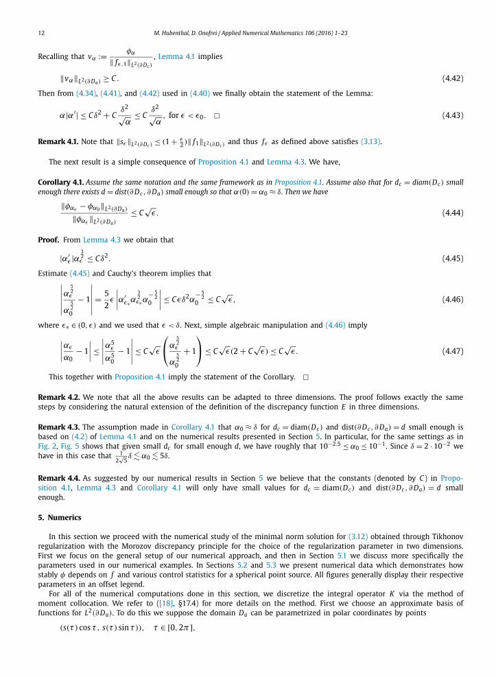

12 M. Hubenthal, D. Onofrei / Applied Numerical Mathematics 106 (2016) 1–23

Recalling that vα := φα

‖ fε,1‖L2(∂ Dc)

, Lemma 4.1 implies

‖vα‖L2(∂ Da)≥ C . (4.42)

Then from (4.34), (4.41), and (4.42) used in (4.40) we finally obtain the statement of the Lemma:

α|α′| ≤ Cδ2 + Cδ2

√α

≤ Cδ2

√α

, for ε < ε0. � (4.43)

Remark 4.1. Note that ‖sε‖L2(∂ Dc)≤ (1 + ε

2 )‖ f1‖L2(∂ Dc)and thus fε as defined above satisfies (3.13).

The next result is a simple consequence of Proposition 4.1 and Lemma 4.3. We have,

Corollary 4.1. Assume the same notation and the same framework as in Proposition 4.1. Assume also that for dc = diam(Dc) small enough there exists d = dist(∂ Dc, ∂ Da) small enough so that α(0) = α0 ≈ δ. Then we have

‖φαε − φα0‖L2(∂ Da)

‖φαε ‖L2(∂ Da)

≤ C√

ε. (4.44)

Proof. From Lemma 4.3 we obtain that

|α′ε |α

32ε ≤ Cδ2. (4.45)

Estimate (4.45) and Cauchy’s theorem implies that∣∣∣∣∣∣α52ε

α52

0

− 1

∣∣∣∣∣∣= 5

2ε

∣∣∣∣α′ε∗α

32ε∗α

− 52

0

∣∣∣∣≤ Cεδ2α− 5

20 ≤ C

√ε, (4.46)

where ε∗ ∈ (0, ε) and we used that ε < δ. Next, simple algebraic manipulation and (4.46) imply∣∣∣∣αε

α0− 1

∣∣∣∣≤∣∣∣∣∣α5

ε

α50

− 1

∣∣∣∣∣≤ C√

ε

⎛⎝α52ε

α52

0

+ 1

⎞⎠≤ C√

ε(2 + C√

ε) ≤ C√

ε. (4.47)

This together with Proposition 4.1 imply the statement of the Corollary. �Remark 4.2. We note that all the above results can be adapted to three dimensions. The proof follows exactly the same steps by considering the natural extension of the definition of the discrepancy function E in three dimensions.

Remark 4.3. The assumption made in Corollary 4.1 that α0 ≈ δ for dc = diam(Dc) and dist(∂ Dc, ∂ Da) = d small enough is based on (4.2) of Lemma 4.1 and on the numerical results presented in Section 5. In particular, for the same settings as in Fig. 2, Fig. 5 shows that given small dc for small enough d, we have roughly that 10−2.5 ≤ α0 ≤ 10−1. Since δ = 2 · 10−2 we have in this case that 1

2√

5δ � α0 � 5δ.

Remark 4.4. As suggested by our numerical results in Section 5 we believe that the constants (denoted by C ) in Propo-sition 4.1, Lemma 4.3 and Corollary 4.1 will only have small values for dc = diam(Dc) and dist(∂ Dc, ∂ Da) = d small enough.

5. Numerics

In this section we proceed with the numerical study of the minimal norm solution for (3.12) obtained through Tikhonov regularization with the Morozov discrepancy principle for the choice of the regularization parameter in two dimensions. First we focus on the general setup of our numerical approach, and then in Section 5.1 we discuss more specifically the parameters used in our numerical examples. In Sections 5.2 and 5.3 we present numerical data which demonstrates how stably φ depends on f and various control statistics for a spherical point source. All figures generally display their respective parameters in an offset legend.

For all of the numerical computations done in this section, we discretize the integral operator K via the method of moment collocation. We refer to ([18], §17.4) for more details on the method. First we choose an approximate basis of functions for L2(∂ Da). To do this we suppose the domain Da can be parametrized in polar coordinates by points

(s(τ ) cosτ , s(τ ) sinτ )), τ ∈ [0,2π ],

M. Hubenthal, D. Onofrei / Applied Numerical Mathematics 106 (2016) 1–23 13

Fig. 5. Plot of α0 with respect to k and μ with δ = 0.02.

where s :R →R+ is a 2π -periodic smooth function. Using these coordinates, any function φ defined on ∂ Da can be realized via the pullback as a function of τ :

φ(s(τ ) cosτ , s(τ ) sinτ ).

For convenience, let us use the notation τ̂ = (cosτ , sinτ ) and τ̂⊥ = (− sinτ , cosτ ).Now let na ∈ N and let τ j = 2π j

na, 0 ≤ j ≤ na − 1 be na equally spaced points on the interval [0, 2π). We then use the

exponential basis functions {eilτ }na−1l=0 for L2([0, 2π ]) and approximate a given φ ∈ L2(∂ Da) via interpolation at the points

{τ j}na−1j=0 ⊂ [0, 2π ]. Note that

∫∂ Da

φ(y)∂�

∂νy(x, y)dSy =

2π∫0

φ(s(τ ) cosτ , s(τ ) sinτ )∂�

∂νy(x, (s(τ ) cosτ , s(τ ) sinτ ))

·√

s(τ )2 + s′(τ )2 dθ. (5.1)

Furthermore, since (s′(τ ) cosτ − s(τ ) sinτ , s(τ ) cosτ + s′(τ ) sinτ

)is a tangent vector to ∂ Da , we have that

ν(y) = ν(τ ) = (s(τ ) cosτ + s′(τ ) sinτ , s(τ ) sinτ − s′(τ ) cosτ )√s(τ )2 + s′(τ )2

= s(τ )τ̂ − s′(τ )τ̂⊥√s(τ )2 + s′(τ )2

is the unit outward normal vector to ∂ Da . It is then straightforward to compute in the case of the Helmholtz equation in 2D that

∂�

∂νy(x, (s(τ ) cosτ , s(τ ) sinτ ))

= ∇y�(x, (s(τ ) cosτ , s(τ ) sinτ )) · ν(τ )

= ik

4H(1)′

0 (k|x − s(τ )τ̂ |) s(τ )τ̂ − x√s(τ )2 + |x|2 − 2s(τ )x · τ̂ · s(τ )τ̂ − s′(τ )τ̂⊥√

s(τ )2 + s′(τ )2.

Let na ∈N be the number of sample points on the antenna, ∂ Da , and let nc ∈N be the total number of sample points on ∂ Dc . Also let nR be the total number of sample points on ∂ B R . We write the 2 × (nc + nR) matrix of points

X := [x1, . . . , xnc+nR ],where each x j is a 2-vector, {x j}nc

j=1 ⊂ ∂ Dc and {x j}nc+nRj=nc+1 ⊂ ∂ B R . Approximations of all the integrals involved are then com-

puted using a standard left endpoint sum with the appropriate quadrature weights. All the numerical examples presented herein take Dc to be an annular sector parametrized by r ∈ [r1, r2] and θ ∈ [θ1, θ2]. See Fig. 6 for details.

14 M. Hubenthal, D. Onofrei / Applied Numerical Mathematics 106 (2016) 1–23

Fig. 6. Antenna and control region geometry used for numerical experiments.

For each 1 ≤ j ≤ nc + nR and each 0 ≤ l ≤ na − 1, we compute K [eilτ ](x j) via the approximation

2π

na

na−1∑m=0

∂�(x j, [s(τm) cos (τm) , s(τm) sinτm]T )

∂νyeilτm

√s(τm)2 + s′(τm)2.

If we fix j and vary l, we see that the above sum is equivalent to computing the discrete Fourier transform of the na-vector

v j :=[

∂�(x j, [s(τm) cosτm, s(τm) sinτm]T )

∂νy

√s(τm)2 + s′(τm)2

]na−1

m=0

, (5.2)

which can be computed efficiently using the Fast Fourier Transform algorithm. In particular, for the vector v j in (5.2)

[K {eilτ }(x j)]na−1l=0 ≈ 2πFFT(v j),

where FFT is defined on na-vectors w = [w1, . . . , wna ]T ∈ Cna by

FFT(w) =⎡⎣ 1

na

na∑j=1

w je2π i( j−1)(l−1)

na

⎤⎦na

l=1

. (5.3)

So the matrix representation of K is then the na × (nc + nR) matrix

A := 2π [FFT(v1), · · · ,FFT(vnc+nR )]. (5.4)

Now, in order to approximately solve the ill-posed problem Kφ = ( f1, f2), we attempt to solve the linear system

K1φ(x j) = f1(x j), 1 ≤ j ≤ nc

K2φ(x j) = f2(x j), nc + 1 ≤ j ≤ nc + nR .

Since A is computed with respect to the functions eilθ , we first consider the approximate coefficients of φ with respect to the finite basis {eilτ }na−1

l=0 , given by

cl := 1

na

na−1∑m=0

e−ilτmφ(s(τm) cos(τm), s(τm) sin(τm))dτ ≈ 1

2π

2π∫0

e−ilτ φ(s(τ ) cos(τ ), s(τ ) sin(τ ))dτ . (5.5)

Let

h = [c0, c1, . . . , cna−1]T ∈Cna .

We then numerically compute the Tikhonov regularized solution

hα := (A∗ A + α I)−1 A∗ f ,

M. Hubenthal, D. Onofrei / Applied Numerical Mathematics 106 (2016) 1–23 15

with α > 0. The solution vector hα yields the approximate coefficients cl of the desired density φ with respect to the functions {eilτ }na−1

l=0 . We obtain the density φα corresponding to hα sampled at the angles τm on ∂ Da by the for-mula

φα(τm) :=na−1∑l=0

[hα]leilτm .

After computing the residual Kφ − f (e.g. for φ = φα), we will then need to compute

E(φα, f ) = 1

‖ f1‖2L2(∂ Dc)

‖K1φ − f1‖2L2(∂ Dc)

+ 1

2π R‖K2φ − f2‖2

L2(∂ B R ).

Recall that the discrepancy function F (α) was defined by

F (α) = E(φα, f ) − δ2, (5.6)

where δ > 0 is a fixed error parameter. As discussed in Section 4, the mapping

α �→ E(φα, f )

is not globally increasing, as can be numerically demonstrated. However, for certain feasible regions of (α, ε), F is increasing. And in this case, there is a unique αδ such that F (αδ) = 0. To find αδ , we use Newton’s method combined with an initial coarse line search to identify a good starting point.

First note that if we split the matrix A into two blocks Anear (nc by na) and Afar (nR by na) so that

A =[

Anear

Afar

],

then [Aφ]1 = Anearφ, [Aφ]2 = Afarφ, and A∗ A = A∗near Anear + A∗

far Afar . In the discretized setting, instead of (3.11) we take

F (α) = 1

‖ f1‖2‖Anearhα − f1‖2

L2(∂ Dc)+ 1

2π R‖Afarhα − f2‖2

L2(∂ B R )− δ2 (5.7)

with

hα = (A∗ A + α I)−1 A∗ f = (A∗near Anear + A∗

far Afar + α I)−1(

A∗near f1 + A∗

far f2

). (5.8)

Then in the same spirit as that presented in [3] for Tikhonov regularization with respect to the standard L2 norm, we compute

F ′(α) = −2α

‖ f1‖2L2(∂ Dc)

Re

(∂hα

∂α, hα

)

+(

1

π R− 2

‖ f1‖2L2(∂ Dc)

)Re

(∂hα

∂α, A∗

far Afarhα − A∗far f2

)(5.9)

∂hα

∂α= −(A∗ A + α I)−1hα, (5.10)

where (·, ·) denotes the L2 inner product on ∂ Da .The function f1 defined on ∂ Dc could be, for example, the trace of a plane wave, or of the fundamental solution to the

Helmholtz equation based at some fixed point x0, i.e. a point source. For this paper, we focus on the case where f1 is a point source and where f2 ≡ 0 on ∂ B R . A spherical point source is represented as

i

4H (1)

0 (k|x − x0|), (5.11)

where x0 is the source point (typically outside of B R ).For such an f1, there are some quantities in which we will be interested so as to determine the effectiveness of a

given density φ in solving the problem Kφ = f . These are: the relative error of Kφ on ∂ Dc which will be indicated by the behavior of F (α); the L2 average of Kφ on ∂ B R ; the relative and absolute stability of φ when applying a small perturbation to f1; the norm of φ on ∂ Da . More explicitly, we will measure√

F (αε)

δ,

1√2π R

‖K2φαε ‖L2(∂ B R ), (5.12)

‖φαε − φα0‖L2(∂ Da)

‖φ ‖ 2, ‖φαε − φα0‖L2(∂ Da)

, (5.13)

α0 L (∂ Da)

16 M. Hubenthal, D. Onofrei / Applied Numerical Mathematics 106 (2016) 1–23

and

‖φαε ‖L2(∂ Da), (5.14)

where φαε is the Tikhonov regularization solution to Kφ = ( f1,ε , 0) with ‖ f1 − f1,ε‖L2(∂ Dc)= ε‖ f1‖L2(∂ Dc)

, and φα0 is the solution with unperturbed f1 with αε and α0 chosen according to the Morozov principle. The Morozov solution α0 and αε

are computed via Newton’s Method using (5.9) and (5.10) such that

E(φα0 , f ) = δ2

E(φαε , fε) = δ2. (5.15)

See also the discussion following (5.6). Recall from (3.13), that when adding noise to the data ( f1, 0), we choose a random perturbation η ∈ L2(∂ Dc) and set

f1,ε = f1 + εη̂‖ f1‖L2(∂ Dc), (5.16)

where ε > 0 represents the relative percentage of noise added. In the discrete case, the noise is chosen to be a complex nc-vector ν whose real and imaginary components are pseudorandom numbers (we used uniformly distributed noise, but any distribution would yield similar results) on the interval (−1, 1). Furthermore, for reproducibility, whenever generating ν using a pseudorandom number generator, we always reset the seed to the same value.

5.1. Parameters used for numerical experiments

Here we describe some of the parameters used for the various numerical experiments presented. In Section 5.3 we always assume that ∂ Da is a circle with radius given by a = 0.01, and that ∂ Dc is a sector of an annulus with θ1 = 3π/4and θ2 = 5π/4. We also take R = 10 in all computational examples. We remark that we always restrict the distance from Dc to Da to be no smaller than 10−3 due to the numerical limitations of our approach. This is due to the fact that Kφ is a singular integral when evaluating at points very near to ∂ Da . Therefore, at points on ∂ Dc that are near ∂ Da the limitations of machine precision become more and more apparent. Numerically, we observed that our direct approach starts to break down near d = dist(∂ Dc, ∂ Da) = 10−4. However, we stress that one could most likely obtain high accuracy in computing Kφ

for d ≤ 10−4 by using the Nyström method as discussed in [18].For the collocation method, we use na = 256 sample points on ∂ Da , and narc1 = 256 points on the inner arc of ∂ Dc ,

with the remaining points chosen so as to keep the quadrature weights approximately constant. Thus for a very thin region, nc ≈ 512. We also take nR = 256 (number of sample points on ∂ B R ). Note that increasing nc or nR will put more emphasis on matching f on ∂ Dc or ∂ B R , respectively. The discrepancy parameter δ used for Tikhonov regularization will typically be fixed at 0.02. The key variables under consideration are d = r1 −a, k, and ε (perturbation parameter for adding noise to f1). All of the plots presented in the following sections involve varying two of the aforementioned parameters and plotting different quantities of interest, as stated in (5.12)–(5.14).

When evaluating the relative change in φ given a perturbation of f1, denoted by fε,1, we remark that for the parameter choices we used, a 0.5% change (ε = 0.005) in f1 yielded a roughly 5% change in φ. However, one must keep in mind that this depends quite a lot on the parameters used. In particular, setting the discrepancy δ = 0.02 in all the simulations had an important effect on the numerical results. If we had used δ = 0.05 instead (which leads to approximately a 5% mismatch on the region ∂ Dc), then the relative change in φ given ε = 0.005 would be noticeably smaller. So ultimately there is a tradeoff between μ, R , k, δ, and ε which is not entirely trivial, but this still can be examined experimentally as we have done.

5.2. Near field stability

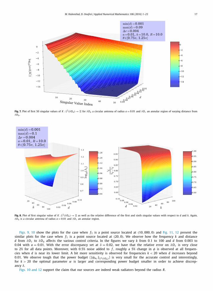
We present below Fig. 7, which shows how the first 50 singular values of the operator K = (K1, K2) vary with d. It is clear that for d small (i.e. for control in the nearfield of the antenna), the rate of decay of the singular values of K is considerably slower than for larger d. This in turn provides some experimental evidence for the fact that nearfield control seems to be more feasible in terms of stable dependence of the solution φ on f . We also show Fig. 8, which shows the behavior of the first and sixth singular value of K with respect to d and k.

5.3. Control for a spherical point source

We now consider the case that

f1(x) = i

4H (1)

0 (k|x − x0|),where x0 is the source point. In all examples presented in this section, we will show plots of the relevant quantities intro-duced at (5.13), (5.14) and we assume R = 10 unless otherwise noted, and x0 = [20, 0]T or x0 = [10000, 0]T (to approximate a source at infinity).

M. Hubenthal, D. Onofrei / Applied Numerical Mathematics 106 (2016) 1–23 17

Fig. 7. Plot of first 50 singular values of K : L2(∂Da) → � for ∂Da a circular antenna of radius a = 0.01 and ∂Dc an annular region of varying distance from ∂Da .

Fig. 8. Plot of first singular value of K : L2(∂Da) → � as well as the relative difference of the first and sixth singular values with respect to d and k. Again, ∂Da is a circular antenna of radius a = 0.01 and ∂Dc an annular region.

Figs. 9, 10 show the plots for the case when f1 is a point source located at (10, 000, 0) and Fig. 11, 12 present the similar plots for the case when f1 is a point source located at (20, 0). We observe how the frequency k and distance d from ∂ Dc to ∂ Da affects the various control criteria. In the figures we vary k from 0.1 to 100 and d from 0.003 to 0.04 with a = 0.01. With the error discrepancy set at δ = 0.02, we have that the relative error on ∂ Dc is very close to 2% for all data points. Moreover, with 0.5% noise added to f , roughly a 5% change in φ is observed at all frequen-cies when d is near its lower limit. A bit more sensitivity is observed for frequencies k < 20 when d increases beyond 0.01. We observe tough that the power budget (‖φαε ‖L2(∂ Da)

) is very small for the accurate control and interestingly, for k > 20 the optimal parameter α is larger and corresponding power budget smaller in order to achieve discrep-ancy δ.

Figs. 10 and 12 support the claim that our sources are indeed weak radiators beyond the radius R .

18 M. Hubenthal, D. Onofrei / Applied Numerical Mathematics 106 (2016) 1–23

Fig. 9. Plot vs. k and d for f1 a spherical point source at x0 = [10000, 0]T .

Fig. 10. Plot of the far field on ∂B R vs. d and ε for f1 a spherical point source at x0 = [10000, 0]T .

It is clear from the figures that for smaller d values the sensitivity of φ to 0.5% noise added to f is close to 5%. As d increases, sensitivity of φ to noise increases as expected. Having x0 nearer or farther from ∂ B R does not have a very significant effect on the overall shape of each subplot.

Figs. 13, 14 show the plots for the case when f1 is a point source located at (10, 000, 0) and Figs. 15, 16 present the similar plots for the case when f1 is a point source located at (20, 0). The numerics indicate how the quantities of interest change with d and the noise factor ε , both with k = 10. The reason for choosing k = 10 instead of, e.g., k = 1 is that from Fig. 9 we see a slightly higher sensitivity of φ to noise for approximately 1 < k < 20 when d starts to increase. So the goal was to capture the worst case scenario for the control stability.

For smaller values of d we see as before that a roughly 0.5% change in f1 yields about a 5% change in φ. Moreover, the dependence on ε for fixed d is superlinear, consistent with the illposedness of the problem. Interestingly, sensitivity of φat d ≈ 0.015 is better than at nearby values, but of course such a value depends on the other parameters of the problem setup. As before, it can be seen in the figures that in both situations our antennas are weak radiators.

M. Hubenthal, D. Onofrei / Applied Numerical Mathematics 106 (2016) 1–23 19

Fig. 11. Plot vs. k and d for f1 a spherical point source at x0 = [20, 0]T .

Fig. 12. Plot of the far field on ∂B R vs. k and d for f1 a spherical point source at x0 = [20, 0]T .

Finally, we consider Fig. 17, which shows the dependence on R and k for a source at x0 = [10000, 0]T . Overall, one can see that R can be decreased to around R = 3 at any frequency between 0.1 and 100 and still achieve the same approximate level of sensitivity for φ as in the previous plots with R = 10.

6. Conclusions and future work

In this paper we studied the feasibility of the active control scheme for the scalar Helmholtz equation. In the L2 setting, we presented analytic conditional stability results as well as detailed 2D numerical sensitivity studies for the minimal energy solution. We provided analytic and 2D numerical arguments for the scheme’s feasibility and broadband character in the near field when the field to be approximated corresponds to an external point source. In Section 2 we highlighted the possible applications of our results for near field synthesis, for the characterization of nonradiating sources with controllable near fields and for Radar Cross-Section (RCS) reduction.

20 M. Hubenthal, D. Onofrei / Applied Numerical Mathematics 106 (2016) 1–23

Fig. 13. Plot vs. d and ε for f1 a spherical point source at x0 = [10000, 0]T .

Fig. 14. Plot of the far field on ∂B R vs. d and ε for f1 a spherical point source at x0 = [10000, 0]T .

We focused our discussion in this paper only on the case of the field to be approximated corresponding to a far field point source (i.e. similar to a plane wave with corresponding decay).

Although we did not include the plots in this paper, we have also numerically studied the case when the interro-gating field is a plane wave without decay or a given uniform field. We observed the scheme does not behave well for the uniform field and that although the stability and accuracy of the near field scheme are essentially independent of the plane wave direction, the overall performance of the scheme is not as good when compared to the case of an interrogating signal coming from a far field observer presented above. In particular, in the case of a nearfield control re-gion as in, e.g., Fig. 13, we observed satisfactory numerical control of a plane wave so long as its direction is not too close to ±π/2, which is related to the shape and orientation of the control region. Moreover, such behavior seems to become more exaggerated as k increases. Also, for the same settings as in Fig. 2 when comparing the case of an in-terrogating far field point source with an interrogating plane wave, we obtained 5% versus 8% stability error and power

M. Hubenthal, D. Onofrei / Applied Numerical Mathematics 106 (2016) 1–23 21

Fig. 15. Plot vs. d and ε for f1 a spherical point source at x0 = [20, 0]T .

Fig. 16. Plot of the far field on ∂B R vs. d and ε for f1 a spherical point source at x0 = [10000, 0]T .

budget levels of ≈ 10−1 versus ≈ 10. We conclude that the scheme performance depends not only on the location of the control region with respect to the source region but also on the amplitude and oscillatory pattern of the incoming field.

Our analysis makes use of Hypothesis 1 which was suggested by the numerics but which we could not prove at this point. Nevertheless we believe that our discussion presents a strong argument for the characterization of almost non-radiating sources with controllable near fields and for the possibility of stable approximation/canceling of unwanted interrogating signals.

Currently we are considering the extension of the sensitivity numerical analysis for scalar fields to 3D and the problem of active manipulation for linear arrays and for large elongated antennas. Then, as a next step in our research efforts, we will work on the extension of the stability analysis to the full Maxwell system in free space.

22 M. Hubenthal, D. Onofrei / Applied Numerical Mathematics 106 (2016) 1–23

Fig. 17. Plot vs. k and R for f1 a spherical point source at x0 = [10000, 0]T .

Acknowledgements

M. Hubenthal was partially supported and D. Onofrei was partially supported by the AFOSR under the 2013 YIP Award FA9550-13-1-0078 and by ONR under the award N00014-15-1-2462.

References

[1] A. Bakushinsky, A. Goncharsky, Ill-Posed Problems: Theory and Applications, Math. Appl., vol. 301, Kluwer Academic Publishers Group, Dordrecht, 1994, Translated from the Russian by I.V. Kochikov.

[2] P.Y. Chen, C. Argyropoulos, A. Alu, Broadening the cloaking bandwidth with non-foster metasurfaces, Phys. Rev. Lett. 111 (2013) 233001.[3] D. Colton, R. Kress, Inverse Acoustic and Electromagnetic Scattering Theory, second edition, Appl. Math. Sci., vol. 93, Springer-Verlag, Berlin, 1998.[4] A.J. Devaney, Nonradiating surface sources, J. Opt. Soc. Am. A 21 (2004).[5] A.J. Devaney, Mathematical Foundation of Imaging, Tomography and Wavefield Inversion, Cambridge University Press, 2012, A Wiley-Interscience Pub-

lication.[6] J. Du, S. Liu, Z. Lin, Broadband optical cloak and illusion created by the low order active sources, Opt. Express 20 (2012) 8608.[7] S. Elliot, P. Nelson, Integral equation methods in scattering theory, Electron. Commun. Eng. J. 2 (1990) 127–136.[8] H.W. Engl, M. Hanke, A. Neubauer, Regularization of Inverse Problems, Math. Appl., vol. 375, Kluwer Academic Publishers Group, Dordrecht, 1996.[9] C. Fuller, A. von Flotow, Active control of sound and vibration, IEEE 15 (1995) 9–19.

[10] F. Guevara Vasquez, G.W. Milton, D. Onofrei, Mathematical analysis of the active exterior cloak for 2d quasistatic electromagnetics, Anal. Math. Phys. 2 (2012) 231–246.

[11] F. Guevara Vasquez, G.W. Milton, D. Onofrei, Active exterior cloaking for the 2d Laplace and Helmholtz equations, Phys. Rev. Lett. 103 (2009) 073901.[12] F. Guevara Vasquez, G.W. Milton, D. Onofrei, Broadband exterior cloaking, Opt. Express 17 (2009) 14800–14805.[13] F. Guevara Vasquez, G.W. Milton, D. Onofrei, Exterior cloaking with active sources in two dimensional acoustics, Wave Motion 48 (2011) 515–524,

Special Issue on Cloaking of Wave Motion.[14] F. Guevara Vasquez, G.W. Milton, D. Onofrei, P. Seppecher, Transformation elastodynamics and active exterior acoustic cloaking, in: R.V. Craster, S. Guen-

neau (Eds.), Acoustic Metamaterials, in: Springer Series in Materials Science, vol. 166, Springer, Netherlands, 2013, pp. 289–318.[15] D. Guicking, Active Control of Sound and Vibration History – Fundamentals – State of the Art, Festschrift DPI, Herausgeber (ed.), Universitatsverlag

Gottingen, 2007.[16] T. Kato, Perturbation Theory for Linear Operators, Classics in Mathematics, Springer-Verlag, Berlin, 1995, Reprint of the 1980 edition.[17] A. Kirsch, An Introduction to the Mathematical Theory of Inverse Problems, second edition, Appl. Math. Sci., vol. 120, Springer, New York, 2011.[18] R. Kress, Linear Integral Equations, third edition, Appl. Math. Sci., vol. 82, Springer, New York, 2014.[19] J. Loncaric, V. Ryaben’kii, S. Tsynkov, Active shielding and control of environmental noise, Technical Report, Institute for Computer Applications in

Science and Engineering (ICASE), 2000.[20] J. Loncaric, S. Tsynkov, Quadratic optimization in the problems of active control of sound, Appl. Numer. Math. 52 (2005) 381–400.[21] P. Lueg, Process of silencing sound oscillations, 1936, US Patent 2,043,416.[22] Q. Ma, Z.L. Mei, S.K. Zhu, T.Y. Jin, T.J. Cui, Experiments on active cloaking and illusion for Laplace equation, Phys. Rev. Lett. 111 (2013) 173901.[23] E. Marengo, A. Devaney, The inverse source problem of electromagnetics: linear inversion formulation and minimum energy solution, IEEE Trans.

Antennas Propag. 47 (1999) 410–412.[24] E. Marengo, A. Devaney, F.K. Gruber, Inverse source problem with reactive power constraint, IEEE Trans. Antennas Propag. 52 (2004) 1586–1595.[25] E. Marengo, R. Ziolkowski, Nonradiating and minimum energy sources and their fields: generalized source inversion theory and applications, IEEE

Trans. Antennas Propag. 48 (2000).

M. Hubenthal, D. Onofrei / Applied Numerical Mathematics 106 (2016) 1–23 23

[26] D.A.B. Miller, On perfect cloaking, Opt. Express 14 (2006) 12457–12466.[27] A.N. Norris, F.A. Amirkulova, W.J. Parnell, Source amplitudes for active exterior cloaking, Inverse Probl. 28 (2012) 105002.[28] H.F. Olson, E.G. May, Electronic sound absorber, J. Acoust. Soc. Am. 25 (1953) 829.[29] D. Onofrei, On the active manipulation of fields and applications: I. The quasistatic case, Inverse Probl. 28 (2012) 105009.[30] D. Onofrei, Active manipulation of fields modeled by the Helmholtz equation, J. Integral Equ. Appl. 26 (2014) 553–579.[31] N. Peake, D. Crighton, Active control of sound, Annu. Rev. Fluid Mech. 32 (2000) 137–164.[32] A. Peterson, S. Tsynkov, Active control of sound for composite regions, SIAM J. Appl. Math. 67 (2007) 1582–1609.[33] B. Popa, D. Shinde, A. Konneker, S. Cummer, Active acoustic metamaterials reconfigurable in real time, Phys. Rev. B 91 (2015).[34] M. Selvanayagam, G. Eleftheriades, An active electromagnetic cloak using the equivalence principle, IEEE Antennas Wirel. Propag. Lett. 11 (2012)

1226–1229.[35] M. Selvanayagam, G.V. Eleftheriades, Experimental demonstration of active electromagnetic cloaking, Phys. Rev. X 3 (2013) 041011.[36] J. Soric, P. Chen, A. Kerkhoff, D. Rainwater, K. Melin, A. Alu, Simulation analysis of an active cancellation stealth system, Optik (2014) 5273–5277.[37] H. Zheng, J. Xiao, Y. Lai, C. Chan, Exterior optical cloaking and illusions by using active sources: a boundary element perspective, Phys. Rev. B 81 (2010)

195116.