ENSCO

Applied Meteorology Unit (AMU)

Quarterly Report

Third Quarter FY-99

Contract NAS10-96018

31 July 1999

ENSCO, Inc. 1980 N. Atlantic Ave., Suite 230

Cocoa Beach, FL 32931 (407) 853-8202 (AMU)

(407) 783-9735

i

Distribution: NASA HQ/Q/F. Gregory NASA HQ/AS/F. Cordova NASA KSC/PH/D. King NASA KSC/PH/R. Roe NASA KSC/AA-C/L. Shriver NASA KSC/AA/R. Bridges NASA KSC/MK/D. McMonagle NASA KSC/PZ-H/H. Silipo NASA KSC/PZ-H-C/D. Frostrum NASA KSC/AA-C-1/J. Madura NASA KSC/AA-C-1/F. Merceret NASA KSC/BL/J. Zysko NASA KSC/MM-E/G. Allen NASA KSC/MM-G/O. Toledo NASA JSC/MA/T. Holloway NASA JSC/ZS8/F. Brody NASA JSC/MS4/J. Richart NASA JSC/MS4/R. Adams NASA JSC/DA8/W. Hale NASA MSFC/EL23/D. Johnson NASA MSFC/EL23/B. Roberts NASA MSFC/SA0-1/A. McCool NASA MSFC/EL23/S. Pearson 45 WS/CC/D. Urbanski 45 WS/DOR/W. Tasso 45 WS/SY/D. Harms 45 WS/SYA/B. Boyd 45 RANS/CC/S. Liburdi 45 OG/CC/P. Benjamin 45 LG/CC/B. Evans 45 LG/LGQ/R. Fore CSR 1300/M. Maier CSR 4140/H. Herring 45 SW/SESL/D. Berlinrut SMC/CWP/Coolidge SMC/CWP/J. Rodgers SMC/CWP/T. Knox SMC/CWP/R. Bailey SMC/CWP (PRC)/P. Conant Hq AFSPC/DORW/S. Carr Hq AFMC/DOW/P. Yavosky Hq AFWA/CC/C. French Hq AFWA/DNX/R. Lefevre Hq AFWA/DN/N. Feldman Hq USAF/XOW/F. Lewis Hq AFRL/XPPR/B. Bauman Office of the Federal Coordinator for Meteorological Services and Supporting Research SMC/SDEW/B. Hickel SMC/MEEV/G. Sandall NOAA “W/OM”/L. Uccellini NOAA/OAR/SSMC-I/J. Golden NOAA/ARL/J. McQueen

ii

NOAA Office of Military Affairs/L. Freeman University of Berkeley – ROTC/T. Adang NWS Melbourne/B. Hagemeyer NWS Southern Region HQ/“W/SRH”/X. W. Proenza NWS Southern Region HQ/“W/SR3”/D. Smith NSSL/D. Forsyth NWS/“W/OSD5”/B. Saffle FSU Department of Meteorology/P. Ray NCAR/J. Wilson NCAR/Y. H. Kuo 30 WS/CC/C. Davenport 30 WS/SYR/S. Sambol 30 SW/XP/R. Miller NOAA/ERL/FSL/J. McGinley SMC/CLNER/B. Kempf Aerospace Corp./B. Lundblad Tetratech/NUS Corp./H. Firstenberg The Weather Channel/G. Forbes ENSCO Contracts/F. Warchal

1

Executive Summary

This report summarizes AMU activities for the third quarter of Fiscal Year (FY) 99 (April - June 1999). A detailed project schedule is included in the Appendix.

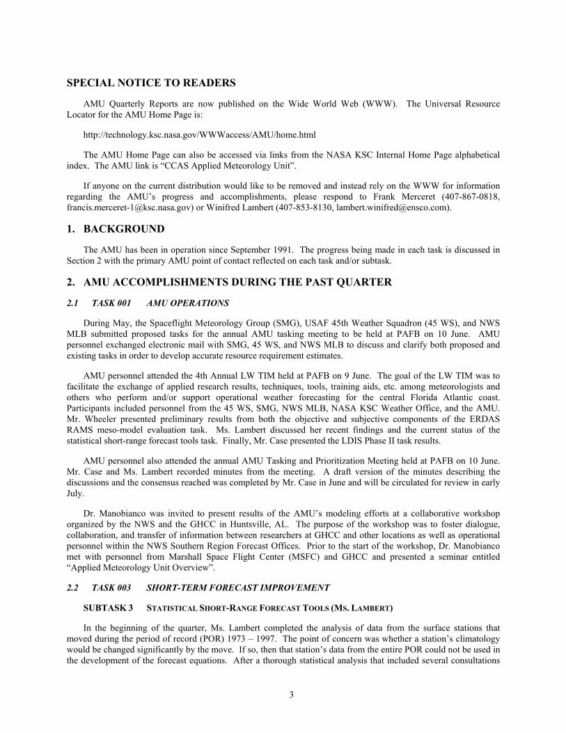
AMU personnel attended the annual AMU Tasking and Prioritization Meeting held at Patrick Air Force Base (PAFB) on 10 June. A draft version of the minutes describing the discussions and the tasks on which consensus was reached has been distributed. A summary of the new tasks to be executed by the AMU is given in the following table.

Task Name Product Sought Operational Benefit Target Begin Date

Target Completion

Date

Extend ERDAS RAMS Evaluation

− Tools to evaluate RAMS quality in real-time

− Training on use of tools − Evaluation of performance

for various weather elements

− Recommendations on improving RAMS

− Final Report documenting all of the above

− Need to advise Range Safety on quality of RAMS

− Seize opportunity for improved local forecasting

Jul 99 Dec 00

WSR-74C IRIS Exploitation

(Phase 1)

− Report or memo outlining prioritized suggestions for IRIS products

− Fully exploit Integrated Radar Information System (IRIS) capabilities

Oct 99 Jan 00

WSR-74C IRIS Exploitation

(Phase 2)

− Build and implement tools identified in Phase 1

− Provide training on use of products

− Final Report documenting products/tools/training

− Improve forecasting of certain weather phenomena that may not be forecast without access to the developed product

Jan 00 Mar 01

Improve Anvil Forecasting (Phase 1)

− Report on technical feasibility of forecasting anvil

− Consultation on decision to proceed to Phase 2

− Improve anvil forecasting for flight rules and launch commit criteria

Oct 99 Mar 00

Local Data Integration System

(Phase 3)

− Assistance in installing and configuring LDIS at customer offices

− Report detailing lessons learned or other notes

− Customers will have access to timely high resolution meteorological data for launch/landing support

Oct 99 Mar 00

Detecting Chaff Source Regions

− Report documenting source regions of chaff affecting radars around KSC during the winter months

− Chaff has negative impact on radar data

− Documentation to show chaff source regions

Oct 99 Jun 00

Ms. Lambert developed preliminary forecast equations for specific ceiling and visibility categories using hourly surface observation data from the National Weather Service in Melbourne (NWS MLB). The overall verificaton scores revealed ambiguous results in skill of the observations-based equations. The poor results may have been caused by using an inappropriate model, multiple linear regression (MLR) in this case. Analysis of the data also revealed that stratification of the data by season might be needed. Future work will include exploratory data analysis to determine relationships between the predictors and predictands and any temporal trends, the addition of data from surrounding stations, and the use of models other than MLR for equation development.

The AMU began an options hours task in April to evaluate the accuracy and reliability of data collected from a “hyper-sodar” by comparing its data to those from the Kennedy Space Center / Cape Canaveral Air Station

2

(KSC/CCAS) wind tower network and 915 MHz profilers. Mr. Palmblad completed the evaluation and a first draft of the final report in June. The final report is currently being circulated for internal review.

In April, the Eastern Range Dispersion Assessment System Regional Atmospheric Modeling System (ERDAS RAMS) evaluation protocol was completed and consists of an objective and subjective component. Preliminary results show that RAMS performs well in forecasting the temperature, wind speed and wind direction at selected wind towers. RAMS was able to forecast 24 out of 25 east-coast sea breeze (ECSB) occurrences and 5 out of 6 non-occurrences. These results indicate that the model is performing well in forecasting ECSB occurrences, however the results are still preliminary due to the small sample size used in the calculations.

Mr. Case continued to work on the real-time Local Data Integration System (LDIS) simulation and sensitivity study. He prepared all the observational and model data needed for ingest into the LDIS, and generated graphical products of primary and derived cloud, wind, and moisture products that have potential value for operations. The final report is currently being written.

Mr. Evans gave a presentation to the Model Verification Program (MVP) Workshop outlining the steps followed in the AMU Option Hours project. He described each model used, their configurations, and how they were initialized. All model output was delivered to the National Oceanic and Atmospheric Administration’s Atmospheric Turbulence Diffusion Laboratory (NOAA ATDL) for analysis. The results will be used to validate and improve the toxic hazard models used by the Eastern and Western Ranges.

AMU personnel attended the 4th Annual Local Weather (LW) Technical Interchange Meeting (TIM) held at PAFB on 9 June. The goal of the LW TIM was to facilitate the exchange of applied research results, techniques, tools, training aids, etc. among meteorologists and others who perform and/or support operational weather forecasting for the central Florida Atlantic coast. Dr. Manobianco was invited to present results of the AMU’s modeling efforts at a collaborative workshop organized by the NWS and the Global Hydrology and Climate Center (GHCC) in Huntsville, AL. The purpose of the workshop was to foster dialogue, collaboration, and transfer of information between researchers at GHCC and other locations as well as operational personnel within the NWS Southern Region Forecast Offices.

During this quarter, Dr. Merceret completed the investigation of the lifetime of upper-air wind features as a function of their vertical size. He developed a technique for correcting measured coherence functions for environment noise and an empirical model for wind coherence as a function of time lag and vertical scale. A first draft of a possible journal article was prepared for internal review.

3

SPECIAL NOTICE TO READERS

AMU Quarterly Reports are now published on the Wide World Web (WWW). The Universal Resource Locator for the AMU Home Page is:

http://technology.ksc.nasa.gov/WWWaccess/AMU/home.html

The AMU Home Page can also be accessed via links from the NASA KSC Internal Home Page alphabetical index. The AMU link is “CCAS Applied Meteorology Unit”.

If anyone on the current distribution would like to be removed and instead rely on the WWW for information regarding the AMU’s progress and accomplishments, please respond to Frank Merceret (407-867-0818, francis.merceret-1@ksc.nasa.gov) or Winifred Lambert (407-853-8130, lambert.winifred@ensco.com).

1. BACKGROUND

The AMU has been in operation since September 1991. The progress being made in each task is discussed in Section 2 with the primary AMU point of contact reflected on each task and/or subtask.

2. AMU ACCOMPLISHMENTS DURING THE PAST QUARTER

2.1 TASK 001 AMU OPERATIONS

During May, the Spaceflight Meteorology Group (SMG), USAF 45th Weather Squadron (45 WS), and NWS MLB submitted proposed tasks for the annual AMU tasking meeting to be held at PAFB on 10 June. AMU personnel exchanged electronic mail with SMG, 45 WS, and NWS MLB to discuss and clarify both proposed and existing tasks in order to develop accurate resource requirement estimates.

AMU personnel attended the 4th Annual LW TIM held at PAFB on 9 June. The goal of the LW TIM was to facilitate the exchange of applied research results, techniques, tools, training aids, etc. among meteorologists and others who perform and/or support operational weather forecasting for the central Florida Atlantic coast. Participants included personnel from the 45 WS, SMG, NWS MLB, NASA KSC Weather Office, and the AMU. Mr. Wheeler presented preliminary results from both the objective and subjective components of the ERDAS RAMS meso-model evaluation task. Ms. Lambert discussed her recent findings and the current status of the statistical short-range forecast tools task. Finally, Mr. Case presented the LDIS Phase II task results.

AMU personnel also attended the annual AMU Tasking and Prioritization Meeting held at PAFB on 10 June. Mr. Case and Ms. Lambert recorded minutes from the meeting. A draft version of the minutes describing the discussions and the consensus reached was completed by Mr. Case in June and will be circulated for review in early July.

Dr. Manobianco was invited to present results of the AMU’s modeling efforts at a collaborative workshop organized by the NWS and the GHCC in Huntsville, AL. The purpose of the workshop was to foster dialogue, collaboration, and transfer of information between researchers at GHCC and other locations as well as operational personnel within the NWS Southern Region Forecast Offices. Prior to the start of the workshop, Dr. Manobianco met with personnel from Marshall Space Flight Center (MSFC) and GHCC and presented a seminar entitled “Applied Meteorology Unit Overview”.

2.2 TASK 003 SHORT-TERM FORECAST IMPROVEMENT

SUBTASK 3 STATISTICAL SHORT-RANGE FORECAST TOOLS (MS. LAMBERT)

In the beginning of the quarter, Ms. Lambert completed the analysis of data from the surface stations that moved during the period of record (POR) 1973 – 1997. The point of concern was whether a station’s climatology would be changed significantly by the move. If so, then that station’s data from the entire POR could not be used in the development of the forecast equations. After a thorough statistical analysis that included several consultations

4

with ENSCO statisticians, she concluded that station moves of approximately a mile or less with minimal changes in elevation did not cause a significant change in climate.

In May, Ms. Lambert began preliminary development of the forecast equations using the method outlined in Vislocky and Fritsch (1997, hereafter VF). In this study, hourly surface observation data were used to develop probability forecasts for the standard flight categories of Low Instrument Flight Rules (LIFR), Instrument Flight Rules (IFR), Marginal Visual Flight Rules (MVFR), and Visual Flight Rules (VFR). Either low ceilings or low visibilities create these categories. VF developed forecast equations for 25 stations in the eastern United States using observational data from the stations themselves and 177 other stations in the region. They also developed persistence climatology forecast equations for each of the categories at the 25 stations using the observations from the forecast sites and a climatic term. These forecasts served as a benchmark against which all other forecast types were compared. All equations were developed using least squares multiple linear regression (MLR) to relate certain variables to the flight categories to be predicted. The observations-based forecasts showed an improvement in skill over persistence climatology when the results were averaged over all 25 stations. The reader is referred to VF for further details.

Ms. Lambert developed the observations-based and persistence climatology equations according to VF. She also developed a basic persistence forecast in which the forecast is equal to the observation at the initial time. Persistence and persistence climatology were used as benchmarks against which the observations-based forecasts were compared. Development of each of the techniques will be discussed separately in the next three sections, and the results from the comparisons will be shown in the final section. In the following discussion, a predictor is a value used to predict the occurrence of a certain flight category, and a predictand is one of the flight categories to be predicted.

Observations-Based Method

To test the observation-based method in VF, Ms. Lambert began by using NWS MLB hourly surface observation data at 1200 UTC to make a one-hour flight category forecast valid at 1300 UTC. Unlike VF, data from other stations were not used in developing the observations-based equations. The data were first divided into an equation-development portion (dependent data set) and an equation-testing portion (independent data set). Of the 25 years of data from 1973 to 1997, 5 years (1974, 1985, 1987, 1990, and 1996) were used as the independent data set and the other years were used as the dependent data set. The data were not stratified any further, i.e. there was no stratification based on season, time of day, month, etc. The next step involved extracting the appropriate data types for the predictors and predictands from the database. Table 1 contains the list of predictands and Table 2 contains the list of predictors used in the development of the equations. These are the same as those found in VF. In Table 1, the flight category is the predictand and the binary threshold is the value that ceiling or visibility must be to create the associated flight category. For any given observation the predictand value will either be 0 if it did not occur or 1 if it did occur.

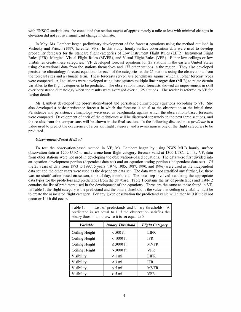
Table 1. List of predictands and binary thresholds. A predictand is set equal to 1 if the observation satisfies the binary threshold, otherwise it is set equal to 0.

Variable Binary Threshold Flight Category

Ceiling Height < 500 ft LIFR Ceiling Height < 1000 ft IFR Ceiling Height ≤ 3000 ft MVFR Ceiling Height > 3000 ft VFR Visibility < 1 mi LIFR Visibility < 3 mi IFR Visibility ≤ 5 mi MVFR Visibility > 5 mi VFR

5

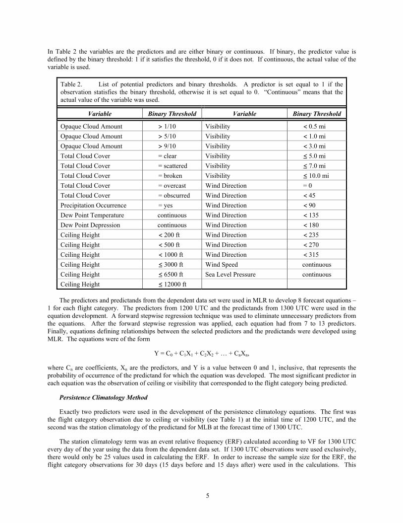
In Table 2 the variables are the predictors and are either binary or continuous. If binary, the predictor value is defined by the binary threshold: 1 if it satisfies the threshold, 0 if it does not. If continuous, the actual value of the variable is used.

Table 2. List of potential predictors and binary thresholds. A predictor is set equal to 1 if the observation statisfies the binary threshold, otherwise it is set equal to 0. “Continuous” means that the actual value of the variable was used.

Variable Binary Threshold Variable Binary Threshold

Opaque Cloud Amount > 1/10 Visibility < 0.5 mi Opaque Cloud Amount > 5/10 Visibility < 1.0 mi Opaque Cloud Amount > 9/10 Visibility < 3.0 mi Total Cloud Cover = clear Visibility ≤ 5.0 mi Total Cloud Cover = scattered Visibility ≤ 7.0 mi Total Cloud Cover = broken Visibility ≤ 10.0 mi Total Cloud Cover = overcast Wind Direction = 0 Total Cloud Cover = obscurred Wind Direction < 45 Precipitation Occurrence = yes Wind Direction < 90 Dew Point Temperature continuous Wind Direction < 135 Dew Point Depression continuous Wind Direction < 180 Ceiling Height < 200 ft Wind Direction < 235 Ceiling Height < 500 ft Wind Direction < 270 Ceiling Height < 1000 ft Wind Direction < 315 Ceiling Height ≤ 3000 ft Wind Speed continuous Ceiling Height ≤ 6500 ft Sea Level Pressure continuous Ceiling Height ≤ 12000 ft

The predictors and predictands from the dependent data set were used in MLR to develop 8 forecast equations – 1 for each flight category. The predictors from 1200 UTC and the predictands from 1300 UTC were used in the equation development. A forward stepwise regression technique was used to eliminate unnecessary predictors from the equations. After the forward stepwise regression was applied, each equation had from 7 to 13 predictors. Finally, equations defining relationships between the selected predictors and the predictands were developed using MLR. The equations were of the form

Y = C0 + C1X1 + C2X2 + … + CnXn,

where Cn are coefficients, Xn are the predictors, and Y is a value between 0 and 1, inclusive, that represents the probability of occurrence of the predictand for which the equation was developed. The most significant predictor in each equation was the observation of ceiling or visibility that corresponded to the flight category being predicted.

Persistence Climatology Method

Exactly two predictors were used in the development of the persistence climatology equations. The first was the flight category observation due to ceiling or visibility (see Table 1) at the initial time of 1200 UTC, and the second was the station climatology of the predictand for MLB at the forecast time of 1300 UTC.

The station climatology term was an event relative frequency (ERF) calculated according to VF for 1300 UTC every day of the year using the data from the dependent data set. If 1300 UTC observations were used exclusively, there would only be 25 values used in calculating the ERF. In order to increase the sample size for the ERF, the flight category observations for 30 days (15 days before and 15 days after) were used in the calculations. This

6

increased the sample size to 620. For example, when calculating the IFR-due-to-ceiling-ERF for 1 July at 1300 UTC, the number of occurrences of IFR in the period 16 June – 16 July would be counted. The total number of occurrences for each category on every day of the year and each time of day was divided by 620, yielding a value between 0 and 1. The ERF value for 1300 UTC 29 February was made equal to the value calculated for 1300 UTC 28 February.

MLR was used to develop a relationship between the two predictors and the predictand at 1300 UTC. The flight category observation at 1200 UTC had a value of either 0 (not observed) or 1 (observed), the ERF was a value between 0 and 1, inclusive. The equation developed produced a value between 0 and 1 that represented the probability of occurrence of the predictand, equivalent to the observations-based method.

Persistence Method

The persistence method assumes that the observation at the forecast time will be the same as that at the initial time. Therefore, if a certain flight category was observed at 1200 UTC, a forecast value of 1 was assigned to that category at 1300 UTC. Otherwise, a value of 0 was assigned.

Preliminary Results

Probability forecasts were made for the data in the dependent and independent data sets using the equations developed by each of the three methods. The Brier Score (B), defined as the average of the squared differences between the observations and the forecasts, was calculated for each forecast method using the equation

2

1

)(1B i

n

ii of

n−= ∑

=

,

where n is the number of observations in the data set, f is the 1300 UTC probability forecast, and o is the 1300 UTC observation (0 or 1).

The Brier Score was used to calculate the percent improvement given by the observations-based forecast over the persistence and persistence climatology forecasts. The percent improvement is also known as the Skill Score (S) and is given by the equation

100)BB(

)BB(S ×−−

=r0

r ,

where B is the observations-based forecast Brier Score, Br is the Brier Score of the reference forecast (persistence or persistence climatology), and B0 is the Brier Score for a perfect forecast. Since the Brier Score is calculated using the difference between the forecast and the observation, B0 is 0. The quantity is multiplied by 100 to yield a percent value. Table 3 shows the results of the Skill Score calculations.

7

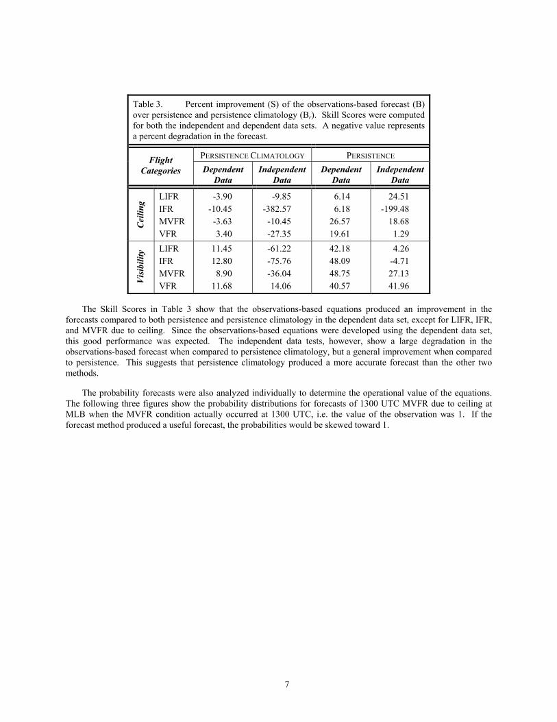
Table 3. Percent improvement (S) of the observations-based forecast (B) over persistence and persistence climatology (Br). Skill Scores were computed for both the independent and dependent data sets. A negative value represents a percent degradation in the forecast.

PERSISTENCE CLIMATOLOGY PERSISTENCE Flight Categories Dependent

Data Independent

Data Dependent

Data Independent

Data

Cei

ling

LIFR IFR MVFR VFR

-3.90 -10.45

-3.63 3.40

-9.85 -382.57

-10.45 -27.35

6.14 6.18

26.57 19.61

24.51 -199.48

18.68 1.29

Vis

ibili

ty LIFR

IFR MVFR VFR

11.45 12.80

8.90 11.68

-61.22 -75.76 -36.04 14.06

42.18 48.09 48.75 40.57

4.26 -4.71 27.13 41.96

The Skill Scores in Table 3 show that the observations-based equations produced an improvement in the forecasts compared to both persistence and persistence climatology in the dependent data set, except for LIFR, IFR, and MVFR due to ceiling. Since the observations-based equations were developed using the dependent data set, this good performance was expected. The independent data tests, however, show a large degradation in the observations-based forecast when compared to persistence climatology, but a general improvement when compared to persistence. This suggests that persistence climatology produced a more accurate forecast than the other two methods.

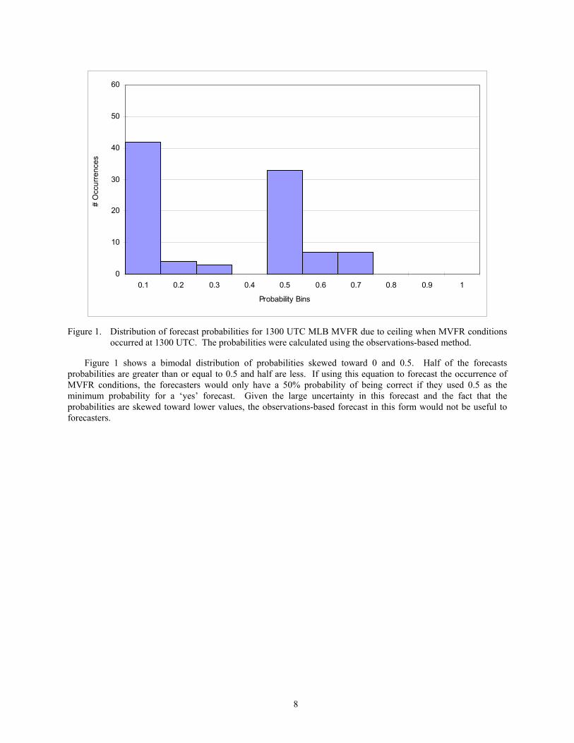
The probability forecasts were also analyzed individually to determine the operational value of the equations. The following three figures show the probability distributions for forecasts of 1300 UTC MVFR due to ceiling at MLB when the MVFR condition actually occurred at 1300 UTC, i.e. the value of the observation was 1. If the forecast method produced a useful forecast, the probabilities would be skewed toward 1.

8

0

10

20

30

40

50

60

0.1 0.2 0.3 0.4 0.5 0.6 0.7 0.8 0.9 1

Probability Bins

# O

ccur

renc

es

Figure 1. Distribution of forecast probabilities for 1300 UTC MLB MVFR due to ceiling when MVFR conditions

occurred at 1300 UTC. The probabilities were calculated using the observations-based method.

Figure 1 shows a bimodal distribution of probabilities skewed toward 0 and 0.5. Half of the forecasts probabilities are greater than or equal to 0.5 and half are less. If using this equation to forecast the occurrence of MVFR conditions, the forecasters would only have a 50% probability of being correct if they used 0.5 as the minimum probability for a ‘yes’ forecast. Given the large uncertainty in this forecast and the fact that the probabilities are skewed toward lower values, the observations-based forecast in this form would not be useful to forecasters.

9

0

10

20

30

40

50

60

0.1 0.2 0.3 0.4 0.5 0.6 0.7 0.8 0.9 1

Probability Bins

# O

ccur

renc

es

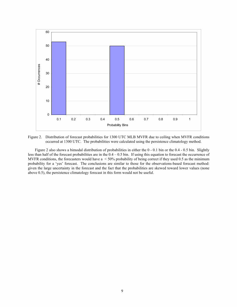
Figure 2. Distribution of forecast probabilities for 1300 UTC MLB MVFR due to ceiling when MVFR conditions

occurred at 1300 UTC. The probabilities were calculated using the persistence climatology method.

Figure 2 also shows a bimodal distribution of probabilities in either the 0 - 0.1 bin or the 0.4 - 0.5 bin. Slightly less than half of the forecast probabilities are in the 0.4 – 0.5 bin. If using this equation to forecast the occurrence of MVFR conditions, the forecasters would have a < 50% probability of being correct if they used 0.5 as the minimum probability for a ‘yes’ forecast. The conclusions are similar to those for the observations-based forecast method: given the large uncertainty in the forecast and the fact that the probabilities are skewed toward lower values (none above 0.5), the persistence climatology forecast in this form would not be useful.

10

0

10

20

30

40

50

60

0.1 0.2 0.3 0.4 0.5 0.6 0.7 0.8 0.9 1

Probability Bins

# O

ccur

renc

es

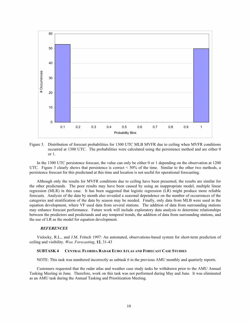
Figure 3. Distribution of forecast probabilities for 1300 UTC MLB MVFR due to ceiling when MVFR conditions

occurred at 1300 UTC. The probabilities were calculated using the persistence method and are either 0 or 1.

In the 1300 UTC persistence forecast, the value can only be either 0 or 1 depending on the observation at 1200 UTC. Figure 3 clearly shows that persistence is correct < 50% of the time. Similar to the other two methods, a persistence forecast for this predictand at this time and location is not useful for operational forecasting.

Although only the results for MVFR conditions due to ceiling have been presented, the results are similar for the other predictands. The poor results may have been caused by using an inappropriate model, multiple linear regression (MLR) in this case. It has been suggested that logistic regression (LR) might produce more reliable forecasts. Analysis of the data by month also revealed a seasonal dependence on the number of occurrences of the categories and stratification of the data by season may be needed. Finally, only data from MLB were used in the equation development, where VF used data from several stations. The addition of data from surrounding stations may enhance forecast performance. Future work will include exploratory data analysis to determine relationships between the predictors and predictands and any temporal trends, the addition of data from surrounding stations, and the use of LR as the model for equation development.

REFERENCES

Vislocky, R.L., and J.M. Fritsch 1997: An automated, observations-based system for short-term prediction of ceiling and visibility. Wea. Forecasting, 12, 31-43

SUBTASK 4 CENTRAL FLORIDA RADAR ECHO ATLAS AND FORECAST CASE STUDIES

NOTE: This task was numbered incorrectly as subtask 6 in the previous AMU monthly and quarterly reports.

Customers requested that the radar atlas and weather case study tasks be withdrawn prior to the AMU Annual Tasking Meeting in June. Therefore, work on this task was not performed during May and June. It was eliminated as an AMU task during the Annual Tasking and Prioritization Meeting.

11

2.3 TASK 004 INSTRUMENTATION AND MEASUREMENT

SUBTASK 5 I&M AND RSA SUPPORT (DR. MANOBIANCO AND MR. WHEELER)

At the request of Mr. Boyd (45 WS) and Col. Harms (45 WS), Dr. Manobianco prepared a briefing entitled “Mesoscale modeling on the Eastern Range in support of weather and safety” that was presented via teleconference to the 83rd Range Commander’s Council Meteorology Group (RCC MG) meeting. The briefing described components of the ERDAS including the configuration, initialization, and evaluation of the RAMS that provides wind forecasts to drive dispersion models. Dr. Manobianco delivered the briefing remotely from the Range Operations Control Center (ROCC) while Col. Harms managed the PowerPoint slides on site at the meeting. Mr. Allan Dianic and Mr. Randy Evans were present with Dr. Manobianco in the ROCC to answer questions about ERDAS RAMS.

SUBTASK 10 EVALUATION OF WIND PROFILER DATA (DR. MANOBIANCO AND MR. PALMBLAD)

NOTE: This task was numbered incorrectly as subtask 5 in the previous three AMU monthly reports. All future AMU monthly and quarterly reports will list the evaluation of wind profiler data described below under Task 4, subtask 10.

The AMU began an options hours task in April 1999 to evaluate the accuracy and reliability of data collected from a “hyper-sodar” for eight days covering the periods 28 October – 2 November 1998 and 16 – 17 March 1999. The evaluation was accomplished using KSC/CCAS wind tower and 915 MHz profiler observations. The primary technical work on the task was performed by Mr. Robert Palmblad (ENSCO, Inc.) and supervised by Dr. Manobianco.

Dr. Manobianco completed the task plan in late April. The 1-minute and 5-minute tower data for all eight days and the 915 MHz profiler data from 16 – 17 March 1999 were obtained from CSR personnel. In addition, Ms. Lambert provided 915 MHz profiler data from 28 October – 2 November 1998 and performed quality control on these data using routines developed for the AMU 915 MHz profiler task. Mr. Palmblad uploaded the sodar, tower, and 915 MHz profiler data to a personal computer (PC) at ENSCO’s Cocoa Beach office and started to examine time series of 5-minute sodar data collected on 17 March 1999.

During May, Mr. Palmblad compared sodar data from 17 March 1999 with Tower 313 and False Cape 915 MHz profiler observations by computing the bias and root mean square (RMS) differences in wind speed and direction as a function of height. He also determined the availability of sodar data as a function of height for the 17 March collection period. The 5-minute sodar data from 17 March have greater temporal and vertical resolution than the 915 MHz profiler data. Therefore, the sodar data were averaged vertically and temporally before computing the bias and RMS to provide a more representative assessment of the accuracy and reliability of the sodar wind measurements.

Mr. Palmblad completed the evaluation and a first draft of the final report in June. The final report is currently being circulated for internal review.

2.4 TASK 005 MESOSCALE MODELING

SUBTASK 4 DELTA EXPLOSION ANALYSIS (MR. EVANS)

The Delta Explosion Analysis project is being funded by KSC under AMU option hours. Mr. Evans is completing revisions of the draft final report on the Delta II explosion. The draft will go to 45 WS and 45 SW for review in July.

SUBTASK 5 MODEL VALIDATION PROGRAM (MR. EVANS)

The primary purpose of the U.S. Air Force’s Model Validation Program (MVP) Data Analysis project, which was funded by option hours from the U.S. Air Force, was to produce RAMS and HYPACT data for the three MVP sessions conducted at Cape Canaveral in 1995-1996. On 11 May Mr. Evans gave a presentation via teleconference

12

to the MVP workshop titled “RAMS & HYPACT modeling for MVP Sessions I, II, & III”. This presentation outlined the steps in the project, which are given below.

Two models were tested in the study: the RAMS and the Hybrid Particle and Concentration Transport (HYPACT) model. RAMS and HYPACT simulations were produced for MVP Sessions I, II, and III.

The RAMS model was run in both the ERDAS and the Parallelized RAMS Operational Weather Simulation System (PROWESS) configurations. The ERDAS configuration used RAMS Version 3a, three nested grids with an innermost grid spacing of 3 km, and no microphysics. The PROWESS configuration used RAMS Version 4a, four nested grids with an innermost grid spacing of 1.5 km, and microphysics. In addition, PROWESS employed a parallel processing technique. Simulations for both configurations were initialized at 0000 and 1200 UTC and produced hourly output.

Both RAMS configurations were initialized with Nested Grid Model (NGM) gridded data when available through the Meteorological Interactive Data Display System (MIDDS). During Session II, however, NGM data were available for only 12 of the 17 days in the Session period due to MIDDS problems. Therefore, PROWESS was initialized using the 2.5 degree National Center for Atmospheric Research/National Center for Environmental Prediction (NCAR/NCEP) Reanalysis data for all 17 days during Session II. However, ERDAS simulations were initialized with the available NGM data only on the 12 days the NGM data was available.

The HYPACT model was initialized with RAMS output data. HYPACT runs were made with both RAMS configurations. The grid domain was 60 X 60 km in the horizontal and 1.5 km in the vertical. The grid spacing was 400 m horizontally and 50 m vertically. The time step used was 180 s (3 min).

The HYPACT-modeled source emission rate and concentrations were calculated in 10-minute increments. For each 10-minute period, the average and standard deviations of the flow rate, latitude, longitude, and heights were calculated. The emission rate corresponded to the flow rate and the shape of the source is determined by the average and standard deviation values of the latitude, longitude, and height. The concentrations were output in parts-per-trillion (ppt) of sulfur hexa-flouride.

RAMS and HYPACT output from all three sessions was sent to the NOAA ATDL for analysis. The results will be used to validate and improve the toxic hazard models used by the Eastern and Western Ranges.

SUBTASK 8 MESO-MODEL EVALUATION (MR. WHEELER AND DR. MANOBIANCO)

ERDAS RAMS Evaluation

In April, the ERDAS RAMS evaluation protocol was completed, reviewed, and approved by the 45 WS, SMG, NWS MLB and NASA. The evaluation protocol consists of an objective and subjective component. The protocol also states that a limited data set will be evaluated. The objective component will focus on the overall accuracy of wind, temperature and moisture at selected sites. The subjective evaluation will verify RAMS forecasts of the onset and movement of the central Florida ECSB, precipitation, and low-level temperature. The subjective verification will be performed by examining RAMS output from both 0000 and 1200 UTC daily model runs. The results presented in the following sections are preliminary and are based on a small sample.

Objective Evaluation

Mr. Dianic of ENSCO, Inc. is performing the objective evaluation of the task. As part of this evaluation, he developed software to analyze the observational and forecast data. These tools compare current and archived model data to surface, upper air, wind tower network, and profiler observational data. Mr. Dianic began computing the bias, mean absolute error, and RMS error of wind speed, wind direction, temperature, and dew point temperature at KSC/CCAS wind towers and standard surface stations. These error statistics will be computed separately for RAMS forecasts initialized at 1200 and 0000 UTC during the months of April through September 1999.

Based on preliminary evaluation results using data collected from April and May 1999, the RAMS model performs well in forecasting the average spatial trends in observed temperature, wind speed and wind direction at selected wind towers. The model tended to underestimate the diurnal temperature cycle at towers 1012 and 509 by approximately 5oC. This systematic error may be related to initializing the soil moisture at a constant value, which

13

was too high during April and May 1999. The AMU will perform additional sensitivity runs with RAMS to determine if the forecast errors are related to soil moisture, grid resolution, or other factors.

Subjective Evaluation

Mr. Wheeler is performing the subjective component of the evaluation that will verify RAMS forecasts of the onset, motion, and depth of the central Florida ECSB across the KSC/CCAS wind tower network, as well as precipitation and low-level temperature. Four worksheets were developed to aid in verifying the model forecasts during the 1999 warm season from 1 May through 1 September. The subjective verification examines RAMS output from both 0000 and 1200 UTC daily model runs. The evaluation usually takes place prior to 0800 EDT and from 1000 – 1300 EDT, Monday through Friday.

As part of the subjective evaluation, 45 WS forecasters and Launch Weather Officers (LWO) are encouraged to participate through discussions of model performance, normally around 0700 and 1200 EDT. These discussions focus on model forecasts of the ECSB and precipitation from the last two RAMS runs. This participation is noted on the AMU worksheets. In June 1999, Mr. Wheeler provided training/guidance on how to call up ERDAS RAMS displays. On several occasions Mr. Pinder of the 45 WS stated he was impressed by the accuracy and timing of the 1-hour precipitation forecasts.

Preliminary results of the subjective evaluation on the May data set were presented at the 4th Annual LW TIM in June. During May, there were 13 observed ECSB days out of 19 days that data were collected. The 915 MHz profiler data were not available for most of the first half of the month due to a change in data formats by the Range Standardization and Automation (RSA) contractor. In addition, the ERDAS RAMS data collection routine does not archive 915 MHz profiler observations when the Weber-Wuertz quality control algorithm identifies bad data. As a result, 915 MHz profiler data were available to evaluate the depth of the ECSB for only 7 days in May. The verification of precipitation was performed for 10 out of 19 days. Initially, there was a problem archiving the 1-hour precipitation product on the Weather Surveillance Radar-1988 Doppler (WSR-88D). To solve this problem, a loop of the 1-hour precipitation product was developed on the AMU’s WSR-88D Principle User Processor (PUP). As long as the PUP communication line to Melbourne stays up, two days worth of data will be available at all times.

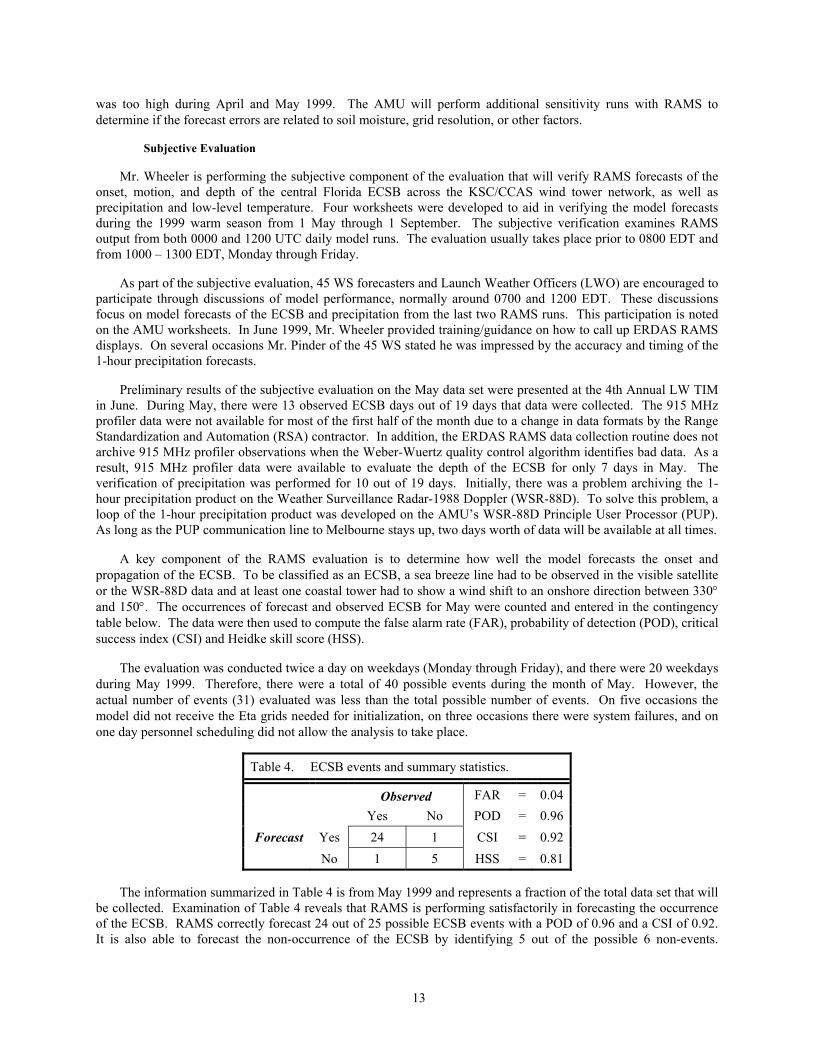
A key component of the RAMS evaluation is to determine how well the model forecasts the onset and propagation of the ECSB. To be classified as an ECSB, a sea breeze line had to be observed in the visible satellite or the WSR-88D data and at least one coastal tower had to show a wind shift to an onshore direction between 330° and 150°. The occurrences of forecast and observed ECSB for May were counted and entered in the contingency table below. The data were then used to compute the false alarm rate (FAR), probability of detection (POD), critical success index (CSI) and Heidke skill score (HSS).

The evaluation was conducted twice a day on weekdays (Monday through Friday), and there were 20 weekdays during May 1999. Therefore, there were a total of 40 possible events during the month of May. However, the actual number of events (31) evaluated was less than the total possible number of events. On five occasions the model did not receive the Eta grids needed for initialization, on three occasions there were system failures, and on one day personnel scheduling did not allow the analysis to take place.

Table 4. ECSB events and summary statistics.

Observed FAR = 0.04 Yes No POD = 0.96

Forecast Yes 24 1 CSI = 0.92 No 1 5 HSS = 0.81

The information summarized in Table 4 is from May 1999 and represents a fraction of the total data set that will be collected. Examination of Table 4 reveals that RAMS is performing satisfactorily in forecasting the occurrence of the ECSB. RAMS correctly forecast 24 out of 25 possible ECSB events with a POD of 0.96 and a CSI of 0.92. It is also able to forecast the non-occurrence of the ECSB by identifying 5 out of the possible 6 non-events.

14

Although the analysis was done using a small sample size (one month), it does show that the model is performing satisfactorily in forecasting the occurrence or non-occurrence of the ECSB. Evaluation of the model’s warm season performance will continue through September 1999. At that time, additional statistical information will be computed and presented in an interim report.

MM5 Evaluation

The NWS MLB requested that the Department of Forestry MM5 evaluation task be withdrawn prior to the AMU annual tasking meeting in June. Therefore, Dr. Manobianco has stopped work on this task.

SUBTASK 9 LOCAL DATA INTEGRATION SYSTEM EXTENSION (MR. CASE)

The real-time LDIS simulation and sensitivity study continued during the past quarter. Following a one-month delay due to the development and modification of the level III WSR-88D remapping algorithm, all other aspects of the project progressed on schedule. The remapping algorithm ingests WSR-88D level III data, as received at SMG, and converts/interpolates the data onto the Advanced Regional Prediction System (ARPS) Data Analysis System (ADAS) grid.

Prior to the real-time LDIS simulation of 15-28 February 1999, Mr. Case completed the preparation of all archived data for the two-week period. He ran conversion and processing programs for all data types within the two-week archive, and corrected problems associated with the surface and rawinsonde conversion algorithms. Also, Mr. Case adjusted the WSR-88D remapping algorithm to run more efficiently.

In addition to preparing all observational data, Mr. Case modified and ran an ADAS pre-processing program that interpolates Rapid Update Cycle (RUC) forecast gridded data onto the 10-km ADAS analysis grid. The RUC 3−6-hr forecasts served as a background, or first guess field, for the subsequent 10-km ADAS analyses. Because RUC data are received at SMG up to 3 hours after the model initialization time, the RUC 3−6-hr forecasts rather than analyses were used as background fields for ADAS in order to simulate a real-time configuration. The RUC data were interpolated to the ADAS analysis grid every 15 minutes corresponding to the frequency of the ADAS analysis cycle. While converting these RUC data onto the ADAS analysis grid, Mr. Case documented the specific times when no RUC forecast was archived. Correspondingly, no analyses were generated for the times when the RUC data were not available. However, this problem could be corrected by using an older RUC or Eta forecast grid as a background field for ADAS. As in LDIS Phase I, once the 10-km ADAS analysis was completed, it served as the background field for the 2-km ADAS analysis grid.

As part of the real-time LDIS simulation, graphical products were routinely generated for both the 10-km and 2-km analysis grids. The graphical products were created using the General Meteorological Package (GEMPAK) software and emphasis was placed on the visualization of primary and derived cloud, wind, and moisture products that have potential value for operations. Among the products included are horizontal and vertical slices of wind speed and direction, divergence, vertical velocity, cloud liquid and ice mixing ratios, precipitation mixing ratios, and relative humidity. Convective parameters and surface temperature plots were also generated. In addition, time-height cross sections of select quantities were produced every six hours. Mr. Case qualitatively examined these products during and after the real-time simulations to determine the potential utility of a real-time LDIS and its derived products.

Sample graphical products from the real-time LDIS simulation were presented at the 4th Annual LW TIM on 9 June. These results will form the basis for additional case studies in the LDIS Phase II Final Report. Emphasis will be placed on specific days that experienced weather of operational interest to SMG.

One of the objectives of this extension task is to determine the influence of level II versus level III WSR−88D data on the subsequent ADAS analyses. The control simulations for the 2-week archive ingested level III data from SMG for all Florida sites. Once the control simulations were completed, Mr. Case re-ran several hours of analyses from 28 February using level II data from the NWS MLB. On 28 February, a pre-frontal line of thunderstorms propagated southeastward across east-central Florida followed by the low-level cold front. The preliminary comparison revealed that the analyses using level II WSR−88D data could adequately resolve both bands of low-level convergence associated with the pre-frontal thunderstorms and the cold front. However, ADAS analyses

15

using the degraded level III WSR-88D data could not resolve the convergence associated with the cold front. These results will be included in the LDIS Phase II Final Report to illustrate the dependence of ADAS analyses on high-quality level II WSR-88D data to adequately resolve subtle mesoscale wind features.

Finally, Mr. Case attended the 8th Conference on Mesoscale Processes in Boulder, CO from 28 June to 1 July. At this conference, he presented a poster that included results from the LDIS Phase I case study of a thunderstorm outflow boundary that scrubbed an Atlas launch operation on 26 July 1997.

2.5 AMU CHIEF’S TECHNICAL ACTIVITIES (DR. MERCERET)

During this quarter, Dr. Merceret completed the investigation of the lifetime of upper-air wind features as a function of their vertical size. He developed a technique for correcting measured coherence functions for environment noise. He also developed an empirical model for wind coherence as a function of time lag and vertical scale. The model produces a power-law relation between coherence time and vertical scale. A first draft of a possible journal article was prepared for internal review. The results will be presented to the Titan Day of Launch Working Group (DOLWG) in July.

16

NOTICE

Mention of a copyrighted, trademarked, or proprietary product, service, or document does not constitute endorsement thereof by the author, ENSCO, Inc., the AMU, the National Aeronautics and Space Administration, or the United States Government. Any such mention is solely for the purpose of fully informing the reader of the resources used to conduct the work reported herein.

17

List of Acronyms

30 SW 30th Space Wing 30 WS 30th Weather Squadron 45 LG 45th Logistics Group 45 OG 45th Operations Group 45 SW 45th Space Wing 45 WS 45th Weather Squadron ADAS ARPS Data Assimilation System AFMC Air Force Materiel Command AFRL Air Force Research Laboratory AFSPC Air Force Space Command AFWA Air Force Weather Agency AMU Applied Meteorology Unit ARPS Advanced Regional Prediction System ATDL Atmospheric Turbulence Diffusion Laboratory CCAS Cape Canaveral Air Station CSI Critical Success Index CSR Computer Science Raytheon ECSB East Coast Sea Breeze EDT Eastern Daylight Time ERDAS Eastern Range Dispersion Assessment System ERF Event Relative Frequency FAR False Alarm Rate FSL Forecast Systems Laboratory FSU Florida State University FY Fiscal Year GEMPAK General Meteorological Package GHCC Global Hydrology and Climate Center HSS Heidke Skill Score HYPACT HYbrid Particle And Concentration Transport I&M Improvement and Modernization IFR Instrument Flight Rules IRIS Integrated Radar Information System JSC Johnson Space Center KSC Kennedy Space Center LDIS Local Data Integration System LIFR Low Instrument Flight Rules LR Logistic Regression LWO Launch Weather Officer LW TIM Local Weather Technical Interchange Meeting

18

List of Acronyms

MHz Mega-Hertz MIDDS Meteorological Interactive Data Display System MLR Multiple Linear Regression MSFC Marshall Space Flight Center MVFR Marginal Visual Flight Rules MVP Model Validation Program NASA National Aeronautics and Space Administration NCAR National Center for Atmospheric Research NCEP National Center for Environment Prediction NGM Nested Grid Model NOAA National Oceanic and Atmospheric Administration NSSL National Severe Storms Laboratory NWS MLB National Weather Service Melbourne PAFB Patrick Air Force Base PC Personal Computer POD Probability of Detection POR Period of Record PROWESS Parallelized RAMS Operational Weather Simulation System PUP Principle User Processor RAMS Regional Atmospheric Modeling System RCC MG Range Commanders Council Meteorology Group RMS Root Mean Square ROCC Range Operations Control Center RSA Range Standardization and Automation RUC Rapid Update Cycle SMC Space and Missile Center SMG Spaceflight Meteorology Group USAF United States Air Force UTC Universal Coordinated Time VF Vislocky and Fritsch VFR Visual Flight Rules WSR-88D Weather Surveillance Radar - 88 Doppler WWW World Wide Web

19

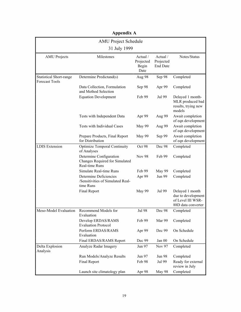
Appendix A

AMU Project Schedule

31 July 1999

AMU Projects Milestones Actual / Projected

Begin Date

Actual / Projected End Date

Notes/Status

Statistical Short-range Forecast Tools

Determine Predictand(s) Aug 98 Sep 98 Completed

Data Collection, Formulation and Method Selection

Sep 98 Apr 99 Completed

Equation Development Feb 99 Jul 99 Delayed 1 month- MLR produced bad results, trying new models

Tests with Independent Data Apr 99 Aug 99 Await completion of eqn development

Tests with Individual Cases May 99 Aug 99 Await completion of eqn development

Prepare Products, Final Report for Distribution

May 99 Sep 99 Await completion of eqn development

LDIS Extension Optimize Temporal Continuity of Analyses

Oct 98 Dec 98 Completed

Determine Configuration Changes Required for Simulated Real-time Runs

Nov 98 Feb 99 Completed

Simulate Real-time Runs Feb 99 May 99 Completed Determine Deficiencies

/Sensitivities of Simulated Real-time Runs

Apr 99 Jun 99 Completed

Final Report May 99 Jul 99 Delayed 1 month due to development of Level III WSR-88D data converter

Meso-Model Evaluation Recommend Models for Evaluation

Jul 98 Dec 98 Completed

Develop ERDAS/RAMS Evaluation Protocol

Feb 99 Mar 99 Completed

Perform ERDAS/RAMS Evaluation

Apr 99 Dec 99 On Schedule

Final ERDAS/RAMS Report Dec 99 Jan 00 On Schedule Delta Explosion Analysis

Analyze Radar Imagery Jun 97 Nov 97 Completed

Run Models/Analyze Results Jun 97 Jun 98 Completed Final Report Feb 98 Jul 99 Ready for external

review in July Launch site climatology plan Apr 98 May 98 Completed

20