APPLIED HYDRODYNAMICS: AN INTRODUCTION324872/Intro.pdf · APPLIED HYDRODYNAMICS: AN INTRODUCTION by...
23
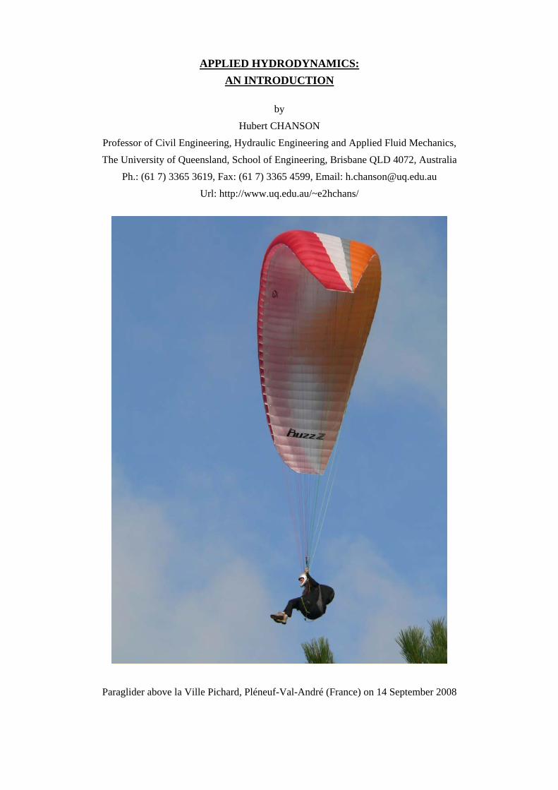
APPLIED HYDRODYNAMICS: AN INTRODUCTION by Hubert CHANSON Professor of Civil Engineering, Hydraulic Engineering and Applied Fluid Mechanics, The University of Queensland, School of Engineering, Brisbane QLD 4072, Australia Ph.: (61 7) 3365 3619, Fax: (61 7) 3365 4599, Email: [email protected] Url: http://www.uq.edu.au/~e2hchans/ Paraglider above la Ville Pichard, Pléneuf-Val-André (France) on 14 September 2008
Transcript of APPLIED HYDRODYNAMICS: AN INTRODUCTION324872/Intro.pdf · APPLIED HYDRODYNAMICS: AN INTRODUCTION by...
APPLIED HYDRODYNAMICS:
AN INTRODUCTION
by
Hubert CHANSON
Professor of Civil Engineering, Hydraulic Engineering and Applied Fluid Mechanics,
The University of Queensland, School of Engineering, Brisbane QLD 4072, Australia
Ph.: (61 7) 3365 3619, Fax: (61 7) 3365 4599, Email: [email protected]
Url: http://www.uq.edu.au/~e2hchans/
Paraglider above la Ville Pichard, Pléneuf-Val-André (France) on 14 September 2008

II
DÉDICACE
To Ya Hui.
Pour Bernard, Nicole et André.
III
TABLE OF CONTENTS
Page
Dédicace II
Table of Contents III
List of Symbols V
Acknowledgments IX
About the author X
Préface XIII
Chapter 1 - Presentation 1
Part I - Irrotational Flow Motion of Ideal Fluid
Chapter I-1 - Introduction to Ideal Fluid Flows I-1-1
Chapter I-2 - Ideal Fluid Flows and Irrotational Flow Motion 1-2-1
Chapter I-3 - Two-Dimensional Flows (1) Basic equations and flow analogies I-3-1
Chapter I-4 - Two-Dimensional Flows (2) Basic flow patterns I-4-1
Chapter I-5 - Complex potential, velocity potential & Joukowski transformation I-5-1
Chapter I-6- Joukowski transformation, theorem of Kutta-Joukowski & lift force on airfoil I-6-1
Chapter I-7 - Theorem of Schwarz-Christoffel, free streamlines & applications I-7-1
Part II - Real Fluid Flows : Theory and Applications
II-1 Introduction II-1

IV
II-2 An introduction to turbulence II-2
II-3 Boundary Layer Theory. Application to Laminar Boundary layer Flows II-3
II-4 Turbulent Boundary layers II-4
Appendices
Appendix A - Glossary - Electronic material A-1
Appendix B - Constants and fluid properties B-1
Appendix C -Unit conversions - Electronic material C-1
Appendix D - Mathematics - Electronic material D-1
Appendix E - The software 2D Flow+ E-1
+ Elecronic download of demonstration version (Electronic material)
Appendix F - Digital video movies F-1
+ Elecronic download / Electronic material (e.g. video streaming)
Assignments
Assignment A - Application to the design of the Alcyone 2 AA-1
Assignment B - Applications to Civil Design on the Gold Coast BB-1
Assignment C - Wind flow past a series of circular buildings CC-1
Assignment D - Prototype freighter Testing DD-1
References R-1
Index of Authors
Index of Subjects
Suggestion/Correction form - Electronic material

V

V
LIST OF SYMBOLS
A cross-section area (m2);
C celerity (m/s);
CD drag coefficient; CD = Drag
12 Vo
2 chord for a two-dimensional object;
CL lift coefficient; CL = Lift
12 Vo
2 chord for a two-dimensional object;
Cc contraction coefficient;
Cd discharge coefficient;
Cv energy loss coefficient;
DH hydraulic diameter (m) :
DH = 4 cross-sectional area
wetted perimeter = 4 APw
d flow depth (m);
e internal energy per unit mass (J/kg);
Fp pressure force (N);
Fv volume force (N);
f Darcy coefficient (or head loss coefficient, friction factor);
fvisc viscous force (N);
g gravity constant (m/s2) : g = 9.80 m/s2 (in Brisbane);
H 1- total head (m) defined as : H = P
g + z +
V2
2 g
2- piezometric head (m) defined as : H = P
g + z
h height (m);
K 1- vortex strength (m2/s) or circulation;
2- hydraulic conductivity (m/s);
k permeability (m2);
k constant of proportionality;
ks equivalent sand roughness height (m);
L length (m);
P absolute pressure (Pa);
Pd dynamic pressure (Pa);
Ps static pressure (Pa);
Q discharge (m3/s);
q discharge per meter width (m2/s);
R 1- circle radius (m);

VI
2- cylinder radius (m);
R1 radius (m);
Ro gas constant : Ro = 8.3143 J/Kmole;
r polar radial coordinate (m);
T thermodynamic (or absolute) temperature (K);
U volume force potential;
V velocity (m/s);
v specific volume (m3/kg) :
v = 1
W complex potential : W = + i;
w complex velocity : w = -Vx + iVy;
x Cartesian coordinate (m);
y Cartesian coordinate (m);
z 1- altitude (m);
2- complex number (Chapters I-5 & I-6);
velocity potential (m2/s);
circulation (m2/s);
specific heat ratio :
= CpCv
1- strength of doublet (m3/s);
2- dynamic viscosity (N.s/m2 or Pa.s);
kinematic viscosity (m2/s) :
=
= 3.141592653589793238462643;
polar coordinate (radian);
density (kg/m3);
surface tension (N/m);
shear stress (Pa);
o average shear stress (Pa);
1- speed of rotation (rad/s);
2- hydrodynamic frequency (Hz) of vortex shedding;
stream function vector; for a two-dimensional flow in the {x,y} plane :
= (0, 0, );
two-dimensional flow stream function (m2/s);
Subscript
n normal component;
VII
o reference conditions : e.g., free-stream flow conditions;
r radial component;
s streamwise component;
x x-component;
y u-component;
z z-component;
ortho-radial component;
Notes :
1- Water at atmospheric pressure and 20.2 Celsius has a kinematic viscosity of exactly 10-6 m2/s.
2- Water in contact with air has a surface tension of about 0.073 N/m.
Dimensionless numbers
Ca Cauchy number (HENDERSON 1966) :
Ca = V2
ECO where Eco is the fluid compressibility;
CD drag coefficient for a structural shape :
CD = o
12 V2
= shear stress
dynamic pressure
where o is the shear stress (Pa);
Note : other notations include Cd and Cf;
Fr Reech-Froude number :
Fr = V
g dcharac
Note : some authors use the notation :
Fr = V2
g dcharac =
V2 A g A dcharac
= inertial force
weight
M Sarrau-Mach number :
M = VC
Nu Nusselt number :
Nu = ht dcharac
= heat transfer by convectionheat transfer by conduction
where ht is the heat transfer coefficient (W/m2/K) and is the thermal conductivity
Re Reynolds number :
Re = V dcharac
= inertial forcesviscous forces
Re* shear Reynolds number :
Re* = V* ks

VIII
St Strouhal number :
St = dcharac
Vo
We Weber number :
We = V2
dcharac
= inertial forces
surface tension forces
Note : some authors use the notation : We = V
dcharac
;
Comments
The variable dcharac characterises the geometric characteristic length (e.g. pipe diameter, flow depth,
sphere diameter, ...).

IX
ACKNOWLEDGEMENTS
The author wants to thank especially Professor Colin J. APELT, University of Queensland, for his
help, support and assistance all along the academic career of the writer. He thanks also Dr Sergio
MONTES, University of Tasmania for his positive feedback and advice on the course material.
He expresses his gratitude to all the people who provided photographs and illustrations of interest,
including:
Mr Jacques-Henri BORDES (France);
Mr and Mrs J. CHANSON (Paris, France);
Mr A. CHANSON (Brisbane, Australia);
Ms Y.H. CHOU (Brisbane, Australia);
Mr Francis FRUCHARD (Lyon,France)
Prof. C. LETCHFORD, University of Tasmania;
Dassault Aviation;
Dryden Aircraft Photo Collection (NASA);
Equipe Cousteau, France;
NASA Earth Observatory;
Northrop Grumman Corporation;
Officine Maccaferri, Italy;
Rafale International;
Stéphane SAISSI (France);
Sequana-Normandie;
VF communication, La Grande Arche;
Vought Retiree Club;
Washington State Department of Transport;
At last, but not the least, the author thanks all the people including students and former students,
professionals, and colleagues who gave him information, feedback and comments on his lecture
material. In particular, he acknowledges : Mr and Mrs J. CHANSON (Paris, France); Ms Y.H. CHOU
(Brisbane, Australia); Mr G. ILLIDGE (University of Queensland); Mrs N. LEMIERE (France);
Professor N. RAJARATNAM (University of Alberta, Canada); Mr R. STONARD (University of
Queensland).

X
ABOUT THE AUTHOR
Hubert CHANSON received a degree of 'Ingénieur Hydraulicien' from the Ecole Nationale Supérieure
d'Hydraulique et de Mécanique de Grenoble (France) in 1983 and a degree of 'Ingénieur Génie
Atomique' from the 'Institut National des Sciences et Techniques Nucléaires' in 1984. He worked for
the industry in France as a R&D engineer at the Atomic Energy Commission from 1984 to 1986, and
as a computer professional in fluid mechanics for Thomson-CSF between 1989 and 1990. From 1986
to 1988, he studied at the University of Canterbury (New Zealand) as part of a Ph.D. project.
Hubert CHANSON is a Professor in hydraulic engineering and applied fluid mechanics at the
University of Queensland since 1990. His research interests include design of hydraulic engineering
and structures, experimental investigations of two-phase flows, coastal hydrodynamics, water quality
modelling, environmental management and natural resources. He authored single-handedly eight
books including: "Hydraulic Design of Stepped Cascades, Channels, Weirs and Spillways"
(Pergamon, 1995), "Air Bubble Entrainment in Free-Surface Turbulent Shear Flows" (Academic
Press, 1997), "The Hydraulics of Open Channel Flow : An Introduction" (Butterworth-Heinemann,
1999 & 2004), "The Hydraulics of Stepped Chutes and Spillways" (Balkema, 2001), "Environmental
Hydraulics of Open Channel Flows" (Elsevier, 2004), "Applied Hydrodynamics: an Introduction to
Ideal and Real Fluid Flows" (CRC Press, 2009) and "Tidal Bores, Aegir, Eagre, Mascaret, Pororoca:
Theory and Observations" (World Scientific, 2011). He co-authored the book "Fluid Mechanics for
Ecologists" (IPC Press, 2002) and he edited several books (Balkema 2004, IEaust 2004, The
University of Queensland 2006,2008,2010, Engineers Australia 2011). His textbook "The Hydraulics
of Open Channel Flow: An Introduction" has already been translated into Chinese (Hydrology Bureau
of Yellow River Conservancy Committee) and Spanish (McGraw Hill Interamericana), and it was re-
edited in 2004. His publication record includes nearly 650 international refereed papers, and his work
was cited over 4,000 times since 1990. Hubert Chanson has been active also as consultant for both
governmental agencies and private organisations. He chaired the Organisation of the 34th IAHR
World Congress held in Brisbane, Australia between 26 June and 1 July 2011.
The International Association for Hydraulic engineering and Research (IAHR) presented Hubert
CHANSON the 13th Arthur Ippen award for outstanding achievements in hydraulic engineering. This
award is regarded as the highest achievement in hydraulic research. The American Society of Civil
Engineers, Environmental and Water Resources Institute (ASCE-EWRI) presented him with the 2004
award for the best practice paper in the Journal of Irrigation and Drainage Engineering ("Energy
Dissipation and Air Entrainment in Stepped Storm Waterway" by CHANSON and TOOMBES 2002).
In 1999 he was awarded a Doctor of Engineering from the University of Queensland for outstanding
research achievements in gas-liquid bubbly flows.

XI
He has been awarded eight fellowships from the Australian Academy of Science. In 1995 he was a
Visiting Associate Professor at National Cheng Kung University (Taiwan R.O.C.) and he was Visiting
Research Fellow at Toyohashi University of Technology (Japan) in 1999 and 2001. In 2008, he was an
invited Professor at the University of Bordeaux (France). In 2004 and 2008, he was a visiting Research
Fellow at Laboratoire Central des Ponts et Chaussées (France). In 2008 and 2010, he was an invited
Professor at the Université de Bordeaux, I2M, Laboratoire des Transferts, Ecoulements, Fluides, et
Energetique, where he is an adjunct research fellow.
Hubert CHANSON was invited to deliver keynote lectures at the 1998 ASME Fluids Engineering
Symposium on Flow Aeration (Washington DC), at the Workshop on Flow Characteristics around
Hydraulic Structures (Nihon University, Japan 1998), at the first International Conference of the
International Federation for Environmental Management System IFEMS'01 (Tsurugi, Japan 2001), at
the 6th International Conference on Civil Engineering (Isfahan, Iran 2003), at the 2003 IAHR Biennial
Congress (Thessaloniki, Greece), at the International Conference on Hydraulic Design of Dams and
River Structures HDRS'04 (Tehran, Iran 2004), at the 9th International Symposium on River
Sedimentation ISRS04 (Yichang, China 2004), at the International Junior Researcher and Engineer
Workshop on Hydraulic Structures IJREW'06 (Montemor-o-Novo, Portugal 2006), at the 2nd
International Conference on Estuaries & Coasts ICEC-2006 (Guangzhou, China 2006), at the 16th
Australasian Fluid Mechanics Conference 16AFMC (Gold Coast, Australia 2007), at the 2008 ASCE-
EWRI World Environmental and Water Resources Congress (Hawaii, USA 2008), the 2nd
International Junior Researcher and Engineer Workshop on Hydraulic Structures IJREW'08 (Pisa,
Italy 2008), the 11th Congrès Francophone des Techniques Laser CTFL 2008 (Poitiers, France 2008),
International Workshop on Environmental Hydraulics IWEH09 (Valencia, Spain 2009), 17th Congress
of IAHR Asia and Pacific Division (Auckland, New Zealand 2010), International Symposium on
Water and City in Kanazawa - Tradition, Culture and Climate (Japan 2010), 2nd International
Conference on Coastal Zone Engineering and Management (Arabian Coast 2010) (Oman 2010), NSF
Partnerships for International Research and Education (PIRE) Workshop on “Modelling of Flood
Hazards and Geomorphic Impacts of Levee Breach and Dam Failure" (Auckland 2012). He gave
invited lectures at the International Workshop on Hydraulics of Stepped Spillways (ETH-Zürich,
2000), at the 2001 IAHR Biennial Congress (Beijing, China), at the International Workshop on State-
of-the-Art in Hydraulic Engineering (Bari, Italy 2004), at the Australian Partnership for Sustainable
Repositories Open Access Forum (Brisbane, Australia 2008), at the 4th International Symposium on
Hydraulic Structures (Porto, Portugal 2012). He lectured several short courses in Australia and
overseas (e.g. Taiwan, Japan, Italy).
His Internet home page is {http://www.uq.edu.au/~e2hchans}. He also developed a gallery of
photographs website {http://www.uq.edu.au/~e2hchans/photo.html} that received more than 2,000 hits
per month since inception. His open access publication webpage is the most downloaded publication
XII
record at the University of Queensland open access repository:
{http://espace.library.uq.edu.au/list.php?browse=author&author_id=193}.
{http://www.uq.edu.au/~e2hchans/photo.html} Gallery of photographs in water
engineering and environmental fluid mechanics
{http://www.uq.edu.au/~e2hchans/url_menu.html} Internet technical resources in water engineering and environmental fluid mechanics
{http://www.uq.edu.au/~e2hchans/reprints.html} Reprints of research papers in water engineering and environmental fluid mechanics
{http://espace.library.uq.edu.au/list.php?browse=author&author_id=193} Open access publications at UQeSpace
Photo - Hubert CHANSON, Professor in Hydraulic Engineering and Applied Fluid Mechanics
XIII
PRÉFACE
Fluid dynamics is the engineering science dealing with forces generated by fluids in motion. Fluid
dynamics and hydrodynamics play a vital role in our everyday life, from the ventilation of our home,
the air flow around cars and aircrafts, wind loads on building. When driving a car, the air flow around
the vehicle body induces some drag which increases with the square of the car speed, contributing to
excess fuel consumption, as well as some downforce used in motor car racing. This advanced
undergraduate and post-graduate textbook is designed especially assist senior undergraduate and
postgraduate students in Aeronautical, Civil, Environmental, Hydraulic and Mechanical Engineering.
The textbook derives from a series of lecture notes developed by the author for the past twenty two
years. The notes were enhanced based upon some extensive feedback from his students as well as
colleagues. The present work draws upon the strength of the acclaimed text "Applied Hydrodynamics:
An Introduction to Ideal and Real Fluid Flows" (CHANSON 2009), with the inclusion of a number of
updates, revisions, corrections, the addition of more exercises, some Internet-based resources
(webpage to be added) and a series of new digial movies available at the book's webpage (webpage to
be added).
Reviews of "Applied Hydrodynamics: An Introduction to Ideal and Real Fluid Flows"
"The book contains a lot of applications and exercises. It handles some aspects in more detail than
other books in hydrodynamics. [...] A great number of the chosen applications comes from phenomena
in nature and from technical applications." (Prof. B. PLATZER, in Z. Angew Math. Mech., 2011, Vol.
91, No. 5, p. 399.)
"This book merits being read and even studied by a very large spectrum of people who should be able
to find it on the shelves of the professional and university libraries that respect themselves. [...] There
is an abyss of ignorance concerning Hydrodynamics bases. [...] This population of modellers [the
users of commercial hydraulics simulation software] receive now, with Hubert Chanson’s book, a tool
for such understanding as well as the material for individual catching up with desired knowledge
profile." (Dr. J. CUNGE, in Journal of Hydraulic Research, 2013, Vol. 51, No. 1, pp. 109-110.)
"Professor Chanson’s book will be an important addition to the field of hydrodynamics. I am glad to
recommend it to instructors, students, and researchers who are in need of a clear and updated
presentation of the fundamentals of fluid mechanics and their applications to engineering practice."
(Dr. O. CASTRO-ORGAZ, in Journal of Hydraulic Engineering, 2013, Vol. 139, No. 4, p. 460.)
1
CHAPTER 1
PRESENTATION
Summary
The thrust of the textbook is presented and discussed. Then, after a short paragraph on fluid properties,
the fundamental equations of real fluid flows are detailed. The particular case of ideal fluid is
presented in the next chapter (Chap. I-1).
1. Presentation
Fluid dynamics is the engineering science dealing with forces and energies generated by fluids in
motion. The study of hydrodynamics involves the application of the fundamental principles of
mechanics and thermodynamics to understand the dynamics of fluid flow motion. Fluid dynamics and
hydrodynamics play a vital role in everyday lives. Practical examples include the flow motion in the
kitchen sink, the exhaust fan above the stove, and the air conditioning system in our home. When we
drive a car, the air flow around the vehicle body induces some drag which increases with the square of
the car speed and contributes to fuel consumption. Engineering applications encompass fluid transport
in pipes and canals, energy generation, environmental processes and transportation (cars, ships,
aircrafts). Other applications includes coastal structures, wind flow around buildings, fluid circulations
in lakes, oceans and atmosphere (Fig. 1), even fluid motion in the human body. Further illustrations
are presented in Appendix F in the form of movies accessible through the publisher’s website.
Civil, environmental and mechanical engineers require basic expertise in hydrodynamics, turbulence,
multiphase flows and water chemistry. The education of these fluid dynamic engineers is a challenge
for present and future generations. Although some introduction course is offered at undergraduate
levels, most hydrodynamic subjects are offered at postgraduate levels only, and they rarely develop the
complex interactions between air and water. Too many professionals and government administrators
do not fully appreciate the complexity of fluid flow motion, nor the needs for further higher education
of quality. Today's engineering problems require engineers with hydrodynamic expertise for a broad
range of situations spanning from design and evaluation to maintenance and decision-making. These
challenges imply a sound understanding of the physical processes and a solid grasp of the physical
laws governing fluid flow motion.
2
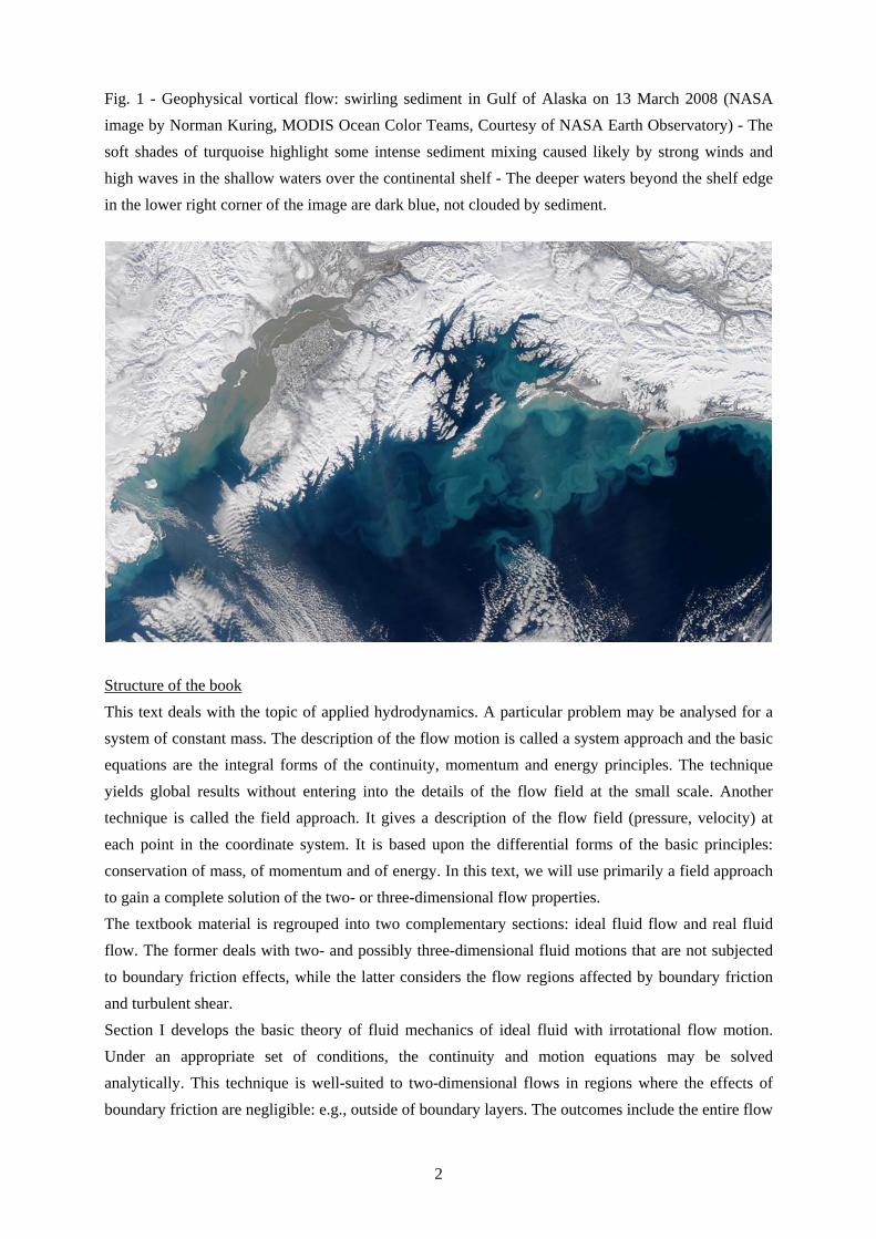
Fig. 1 - Geophysical vortical flow: swirling sediment in Gulf of Alaska on 13 March 2008 (NASA
image by Norman Kuring, MODIS Ocean Color Teams, Courtesy of NASA Earth Observatory) - The
soft shades of turquoise highlight some intense sediment mixing caused likely by strong winds and
high waves in the shallow waters over the continental shelf - The deeper waters beyond the shelf edge
in the lower right corner of the image are dark blue, not clouded by sediment.
Structure of the book
This text deals with the topic of applied hydrodynamics. A particular problem may be analysed for a
system of constant mass. The description of the flow motion is called a system approach and the basic
equations are the integral forms of the continuity, momentum and energy principles. The technique
yields global results without entering into the details of the flow field at the small scale. Another
technique is called the field approach. It gives a description of the flow field (pressure, velocity) at
each point in the coordinate system. It is based upon the differential forms of the basic principles:
conservation of mass, of momentum and of energy. In this text, we will use primarily a field approach
to gain a complete solution of the two- or three-dimensional flow properties.
The textbook material is regrouped into two complementary sections: ideal fluid flow and real fluid
flow. The former deals with two- and possibly three-dimensional fluid motions that are not subjected
to boundary friction effects, while the latter considers the flow regions affected by boundary friction
and turbulent shear.
Section I develops the basic theory of fluid mechanics of ideal fluid with irrotational flow motion.
Under an appropriate set of conditions, the continuity and motion equations may be solved
analytically. This technique is well-suited to two-dimensional flows in regions where the effects of
boundary friction are negligible: e.g., outside of boundary layers. The outcomes include the entire flow

3
properties (velocity magnitude and direction, pressure) at any point. Although no ideal fluid actually
exists, many real fluids have small viscosity and the effects of compressibility may be negligible. For
fluids of low viscosity the viscosity effects are appreciable only in a narrow region surroundings the
fluid boundaries. For incompressible flow where the boundary layer remains thin, non-viscous fluid
results may be applied to real fluid to a satisfactory degree of approximation. Applications include the
motion of a solid through an ideal fluid which is applicable with slight modification to the motion of
an aircraft through the air, of a submarine through the oceans, flow through the passages of a pump or
compressor, or over the crest of a dam, and some geophysical flows. While the complex notation is
introduced in the chapters I-5 to I-7, it is not central to the lecture material and could be omitted if the
reader is not familiar with complex variables.
Fig. 3 - Paraglider above Dune du Pilat (France) on 7 Sept. 2008
In Nature, three types of shear flows are encountered commonly: (1) jets and wakes, (2) developing
boundary layers, and (3) fully-developed open channel flows. Section II presents the basic boundary
layer flows and shear flows. The fundamentals of boundary layers are reviewed. The results are
applied to both laminar and turbulent boundary layers. Basic shear flow and jet applications are
developed. The text material aims to emphasise the inter-relation between ideal and real-fluid flows.
For example, the calculations of an ideal flow around a circular cylinder are presented in Chapter I-4
and compared with real-fluid flow results. Similarly, the ideal fluid flow equations provide the
boundary conditions for the developing boundary layer flows (Chap. II-3 and II-4). The calculations of

4
lift force on air foil, developed for ideal-fluid flows (Chap. I-6), give good results for real-fluid flow
past a wing at small to moderate angles of incidence (Fig. 2).
The lecture material is supported by a series of appendices (A to F), while some major homework
assignments are developed before the bibliographic references. The appendices include some basic
fluid properties, unit conversion tables, mathematical aids, an introduction to an ideal-fluid flow
software, and some presentation of relevant video movies.
Computational fluid dynamics (CFD) is largely ignored in the book. It is a subject in itself and its
inclusion would yield a too large material for an intermediate textbook. In many universities,
computational fluid dynamics is taught as an advanced postgraduate subject for students with solid
expertise and experience in fluid mechanics and hydraulics. In line with the approach of LIGGETT
(1994), this book aims to provide a background for studying and applying CFD.
The lecture material is designed as an intermediate course in fluid dynamics for senior undergraduate
and postgraduate students in Civil, Environmental, Hydraulic and Mechanical Engineering. Basic
references on the topics of Section I include STREETER (1948) and VALLENTINE (1969). The first
four chapters of the latter reference provides some very pedagogical lecture material for simple flow
patterns and flow net analysis. References on the topics of real fluid flows include SCHLICHTING
(1979) and LIGGETT (1994). Relevant illustrations of flow motion comprise VAN DYKE (1982),
JSME (1988) and HOMSY (2000,2004)
Warning
Sign conventions differ between various textbooks. In the present manuscript, the sign convention may differ sometimes
from the above references.
2. Fluid Properties
The density of a fluid is defined as its mass per unit volume. All real fluids resist any force tending
to cause one layer to move over another but this resistance is offered only while movement is taking
place. The resistance to the movement of one layer of fluid over an adjoining one is referred to the
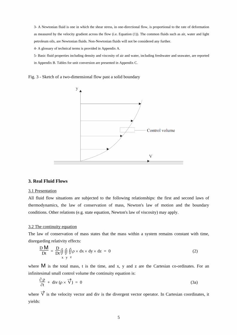
viscosity of the fluid. Newton's law of viscosity postulates that, for the straight parallel motion of a
given fluid, the tangential stress between two adjacent layers is proportional to the velocity gradient in
a direction perpendicular to the layers (Fig. 3):
= Vy
(1)
where is the dynamic viscosity of the fluid.
Notes
1- Isaac NEWTON (1642-1727) was an English mathematician (see Glossary).
2- The kinematic viscosity is the ratio of viscosity to mass density:
=
5
3- A Newtonian fluid is one in which the shear stress, in one-directional flow, is proportional to the rate of deformation
as measured by the velocity gradient across the flow (i.e. Equation (1)). The common fluids such as air, water and light
petroleum oils, are Newtonian fluids. Non-Newtonian fluids will not be considered any further.
4- A glossary of technical terms is provided in Appendix A.
5- Basic fluid properties including density and viscosity of air and water, including freshwater and seawater, are reported
in Appendix B. Tables for unit conversion are presented in Appendix C.
Fig. 3 - Sketch of a two-dimensional flow past a solid boundary
3. Real Fluid Flows
3.1 Presentation
All fluid flow situations are subjected to the following relationships: the first and second laws of
thermodynamics, the law of conservation of mass, Newton's law of motion and the boundary
conditions. Other relations (e.g. state equation, Newton's law of viscosity) may apply.
3.2 The continuity equation
The law of conservation of mass states that the mass within a system remains constant with time,
disregarding relativity effects:
D M
Dt = DDt
x
y
z
dx dy dz = 0 (2)
where M is the total mass, t is the time, and x, y and z are the Cartesian co-ordinates. For an
infinitesimal small control volume the continuity equation is:
t
+ div ( V
) = 0 (3a)
where V
is the velocity vector and div is the divergent vector operator. In Cartesian coordinates, it
yields:
6
t
+ i=x,y,z
( ) Vixi
= 0 (3b)
where Vx, Vy and Vz are the velocity components in the x-, y- and z-directions respectively.
For an incompressible flow (i.e. = constant) the continuity equation becomes:
div V
= 0 (4a)
and in Cartesian coordinates:
i=x,y,z
Vixi
= 0 (4b)
Notes
1- The word Cartesian is named after the Frenchman DESCARTES (App. A). It is spelled with a capital C. René
DESCARTES (1596-1650) was a French mathematician, scientist, and philosopher who is recognised as the father of
modern philosophy.
2- In Cartesian coordinates, the velocity components are Vx, Vy, Vz :
V
= (Vx, Vy, Vz)
3- The vector notation is used herein to lighten the mathematical writings. The reader will find some relevant
mathematical aids in Appendix C.
4- For a two-dimensional and incompressible flow the continuity equations is :
Vxx
+ Vyy
= 0
5- Considering an incompressible fluid flowing in a pipe the continuity equation may be integrated between two cross
sections of areas A1 and A2. Denoting V1 and V2 the mean velocity across the sections, we obtain:
Q = V1 A1 = V2 A2
The above relationship is the integral form of the continuity equation.
3.3 The motion equation
3.3.1 Equation of motion
Newton's second law of motion is expressed for a system as:
DDt ( )M V
= F
(5)
where F
refers to the resultant of all external forces acting on the system, including body forces
such as gravity, and V
is the velocity of the centre of mass of the system. The forces acting on the
control volume are (a) the surface forces (i.e. shear forces) and (b) the volume force (i.e. gravity). For
an infinitesimal small volume, the momentum equation is applied to the i-component of the vector
equation :
7
D ( ) Vi
Dt =
( ) Vi
t +
j=x,y,z Vj
( ) Vixj
= Fvi + j=x,y,z
ijxj
(6)
where Fv is the resultant of the volume forces, is the stress tensor (see Notes below) and i,j = x,y,z.
If the volume forces Fv
are derived from a potential U (U = -gz for the gravity force), they can be
rewritten as:
Fv
= - grad U
(7)
where grad is the gradient vector operator. In Cartesian coordinates, it yields:
Fvx = - Ux
Fvy = - Uy
Fvz = - Uz
For a Newtonian fluid, the shear forces are (1) the pressure forces and (2) the resultant of the viscous
forces on the control volume. Hence, for a Newtonian fluid, the momentum equation becomes:
D ( ) V
Dt = Fv
- grad P
+ f
visc (8a)
where f
visc is the resultant of the viscous forces on the control volume and P is the pressure. In
Cartesian coordinates, it yields:
D ( ) Vi
Dt = Fvi - Pxi
+ fvisci (8b)
Assuming a constant viscosity over the control volume and using the expressions of shear and normal
stresses in terms of the viscosity and velocity gradients, the equation of motion becomes
D ( ) Vi
Dt = Fvi
- Pxi
- 23
j=x,y,z 2 Vjxi xj
+ j=x,y,z
2 Vi
xj xj +
2 Vjxj xi
(8c)
Notes
1- The gravity force equals:
Fv
= - grad
(g z)
U = g
x
where the z-axis is positive upward (i.e. U = g z) and g is the gravity acceleration (Appendix B).
2- The i-component of the vector of viscous forces is:
fi = div i = j=x,y,z
ijxj
8
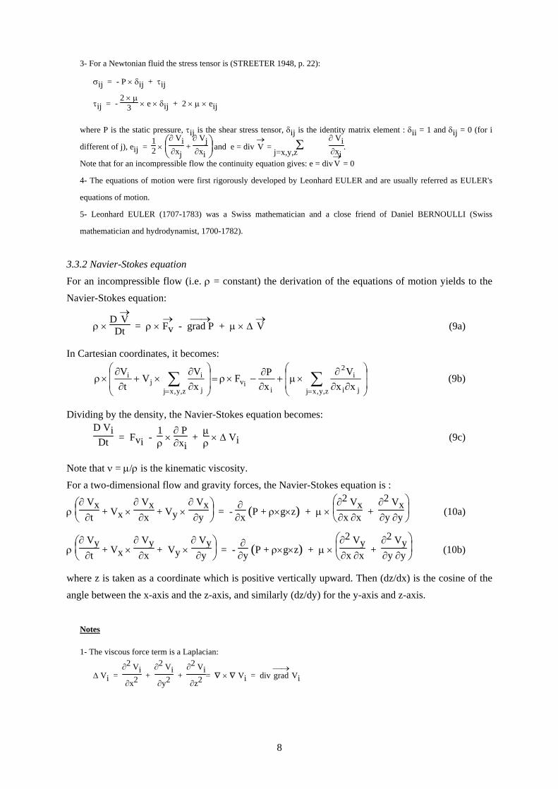
3- For a Newtonian fluid the stress tensor is (STREETER 1948, p. 22):
ij = - P ij + ij
ij = - 2
3 e ij + 2 eij
where P is the static pressure, ij is the shear stress tensor, ij is the identity matrix element : ii = 1 and ij = 0 (for i
different of j), eij = 12
Vi
xj + Vjxi
and e = div V
= j=x,y,z
Vixi
.
Note that for an incompressible flow the continuity equation gives: e = div V
= 0
4- The equations of motion were first rigorously developed by Leonhard EULER and are usually referred as EULER's
equations of motion.
5- Leonhard EULER (1707-1783) was a Swiss mathematician and a close friend of Daniel BERNOULLI (Swiss
mathematician and hydrodynamist, 1700-1782).
3.3.2 Navier-Stokes equation
For an incompressible flow (i.e. = constant) the derivation of the equations of motion yields to the
Navier-Stokes equation:
D V
Dt = Fv
- grad P
+ V
(9a)
In Cartesian coordinates, it becomes:
z,y,xj ji
i2
iiv
z,y,xj j
ij
i
xx
V
x
PF
x
VV
t
V (9b)
Dividing by the density, the Navier-Stokes equation becomes:
D ViDt = Fvi -
1
Pxi
+ Vi (9c)
Note that = / is the kinematic viscosity.
For a two-dimensional flow and gravity forces, the Navier-Stokes equation is :
Vx
t + Vx
Vxx
+ Vy Vxy
= - x
( )P + gz +
2 Vx
x x +
2 Vxy y
(10a)
Vy
t + Vx
Vyx
+ Vy Vyy
= - y
( )P + gz +
2 Vy
x x +
2 Vyy y
(10b)
where z is taken as a coordinate which is positive vertically upward. Then (dz/dx) is the cosine of the
angle between the x-axis and the z-axis, and similarly (dz/dy) for the y-axis and z-axis.
Notes
1- The viscous force term is a Laplacian:
Vi = 2 Vi
x2 + 2 Vi
y2 + 2 Vi
z2 = Vi = div grad
Vi

9
2- The equations were first derived by NAVIER in 1822 and POISSON in 1829 by an entirely different method. They
were derived in a manner similar as above by SAINT-VENANT in 1843 and STOKES in 1845.
3- Henri NAVIER (1785-1835) was a French engineer who primarily designed bridge but also extended EULER's
equations of motion. Siméon Denis POISSON (1781-1840) was a French mathematician and scientist. He developed the
theory of elasticity, a theory of electricity and a theory of magnetism. The Frenchman Adhémar Jean Claude BARRÉ DE
SAINT-VENANT (1797-1886) developed the equations of motion of a fluid particle in terms of the shear and normal
forces exerted on it. George Gabriel STOKES (1819-1903), British mathematician and physicist, is known for his
research in hydrodynamics and a study of elasticity (see Glossary, App. A).