Applied Geostatistics

Miles Logsdonmlog@u.washington.edu

Mimi D’Ioriomimid@u.washington.edu

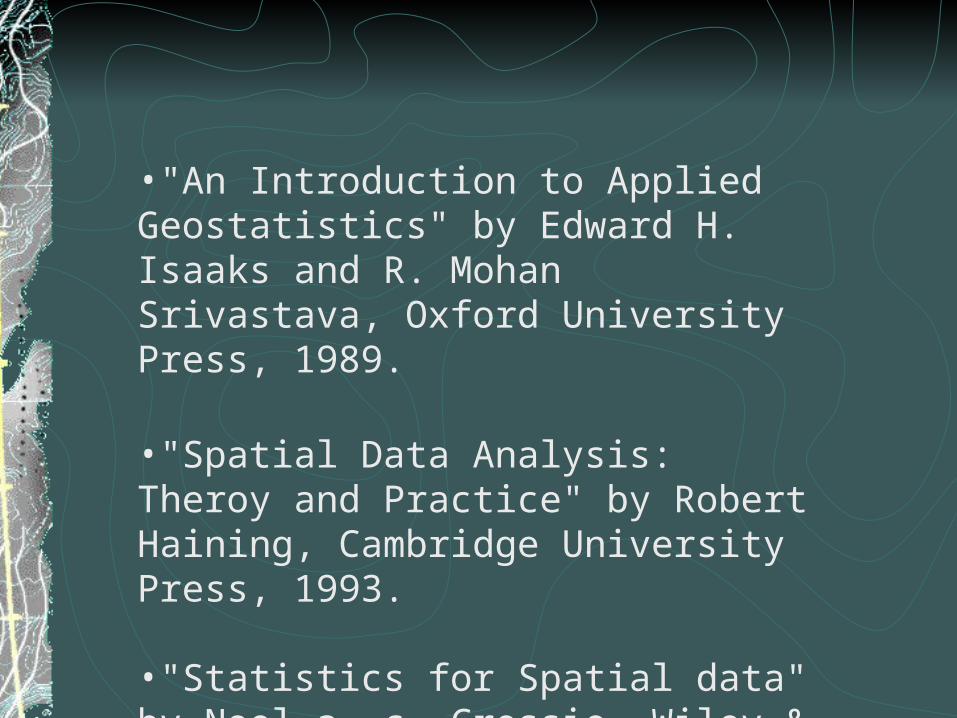
•"An Introduction to Applied Geostatistics" by Edward H. Isaaks and R. Mohan Srivastava, Oxford University Press, 1989.

•"Spatial Data Analysis: Theroy and Practice" by Robert Haining, Cambridge University Press, 1993.

•"Statistics for Spatial data" by Noel a. c. Cressie, Wiley & Sons, Inc. 1991.

Introduction to Geostatistics

Z(s)D • D is the spatial domain or area of

interest

• s contains the spatial coordinates

• Z is a value located at the spatial coordinates

{Z(s): s D}Geostatistics: Z random; D fixed, infinite, continuousLattice Models: Z random; D fixed, finite, (ir)regular gridPoint Patterns: Z 1; D random, finite

GeoStatistics

•Univariate

•Bivariate

•Spatial Description

-A way of describing the spatial continuity as an essential feature of natural phenomena.

- The science of uncertainty which attempts to model order in disorder.

- Recognized to have emerged in the early 1980’s as a hybrid of mathematics, statistics, and mining engineering.

- Now extended to spatial pattern description

Univariate •One Variable•Frequency (table)•Histogram (graph)

•Do the same thing (i.e count of observations in intervals or classes

•Cumulative Frequency (total “below” cutoffs)

Measurements of location (center of distribution

mean (m µ x )medianmode

Measurements of spread (variability)variancestandard deviationinterquartile range

Measurements of shape (symmetry & length

coefficient of skewnesscoefficient of variation

Summary of a histogram

x

n

ii

n

1

2 2

1

1 / n x ii

n

st d. . 2

IQ R Q Q 3 1

C S

nx i

i

n

1 3

12

C V

Bivariate

Scatterplots

X i n

Yi n

p

p

Correlation

p

n i x i yi

n

x y

x y

1

1

Linear Regression

y ax b a p

b a

y

x

y x

slopeconstant

Values at locations that are near to each other are more similar than values at locations that are farther apart.

Autocorrelation

Spatial Description- Data Postings = symbol maps

(if only 2 classes = indicator map- Contour Maps- Moving Windows => “heteroscedasticity”

(values in some region are more variable than in others)- Spatial Continuity

(h-scatterplots * Xj,Yj

tj hij=tj-ti

* Xi,Yi

* ti

(0,0)

Spatial lag = h = (0,1) = same x, y+1

h=(0,0) h=(0,3) h=(0,5)

correlation coefficient(i.e the correlogram, relationship of p with h

Lags

Variograms: How do we estimate them?

21

34

1

2

43

Binning Lags

Variograms: How do we estimate them?

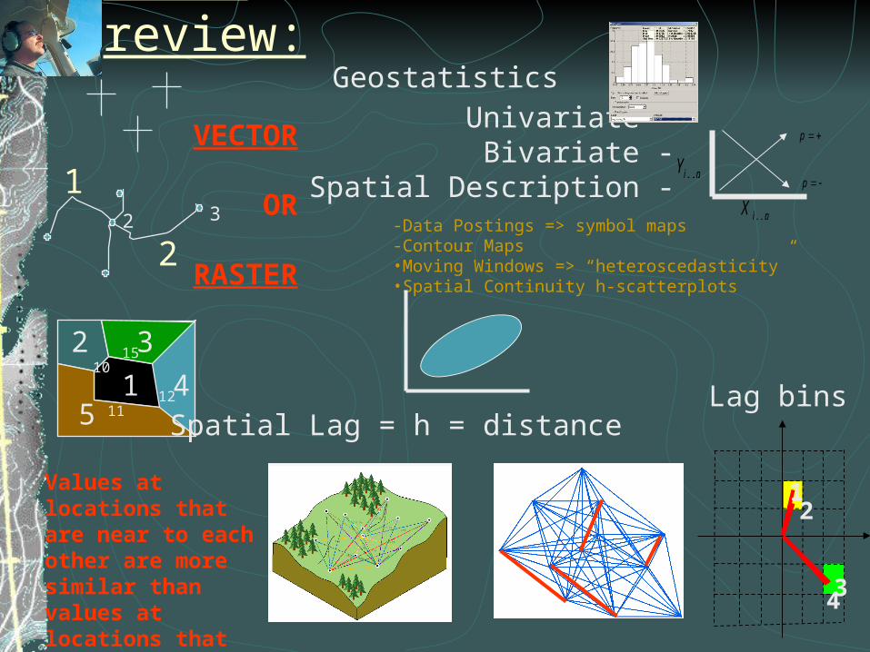
Let’s review:

Univariate -Bivariate -

Spatial Description -

Geostatistics

X i n

Yi n

p

p

1

2 3

45

15

1211

10

2 3

1

2

VECTOR

OR

RASTER

21

34

Spatial Lag = h = distance Lag bins

Values at locations that are near to each other are more similar than values at locations that are farther apart.

= Autocorrelation

-Data Postings => symbol maps-Contour Maps•Moving Windows => “heteroscedasticity”•Spatial Continuity h-scatterplots

Definitions

))()(var()(2

Variogram

)(/)()(

ationAutocorrel

))(),(cov()(

Covariance

hssh

0hh

hssh

ZZ

CC

ZZC

Variograms: What are they?

•Correlogram = p(h) = the relationship of the correlation coefficient of an h-scatterplot and h (the spatial lag)•Covariance = C(h) = the relationship of the coefficient of variation of an h-scatterplot and h•Semivariogram = variogram = = moment of inertia

( )h

1

2

2

1n i ii

n

x ymoment of inertia =

OR: half the average sum difference between the x and y pairof the h-scatterplot

OR: for a h(0,0) all points fall on a line x=y

OR: as |h| points drift away from x=y

Isotropy

Variograms: What are their features?

Anisotropy

Variograms: What are their features?

Anisotropy

Variograms: What are their features?

Anisotropy

Variograms: What are their features?

Represent the Data

Represent the Represent the DataData

Explore the DataExplore the DataExplore the Data

Fit a ModelFit a ModelFit a Model

Perform Diagnostics

Perform Perform DiagnosticsDiagnostics

Compare the Models

Compare the Compare the ModelsModels

Structured Structured Process in Process in GeostatisticsGeostatistics

Physiognomy / Pattern / structure

Composition = The presence and amount of each element type without spatially explicit measures.

Proportion, richness, evenness, diversity

Configuration = The physical distribution in space and spatial character of elements.

Isolation, placement, adjacency

** some metrics do both **

Types of MeticsArea MetricsPatch Density, Size and VariabilityEdge MetricsShape MetricsCore Area MetricsNearest-Neighbor MetricsDiversity MetricsContagion and Interspersion Metrics

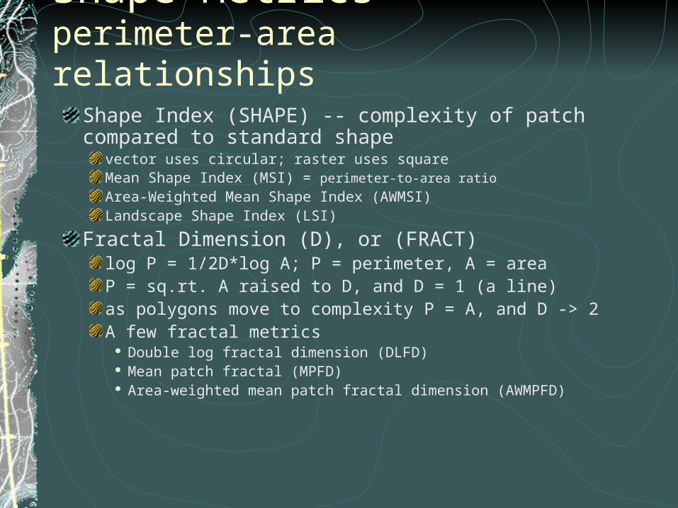
Shape Metricsperimeter-area relationships

Shape Index (SHAPE) -- complexity of patch compared to standard shape

vector uses circular; raster uses squareMean Shape Index (MSI) = perimeter-to-area ratioArea-Weighted Mean Shape Index (AWMSI)Landscape Shape Index (LSI)

Fractal Dimension (D), or (FRACT) log P = 1/2D*log A; P = perimeter, A = areaP = sq.rt. A raised to D, and D = 1 (a line)as polygons move to complexity P = A, and D -> 2A few fractal metrics

Double log fractal dimension (DLFD) Mean patch fractal (MPFD) Area-weighted mean patch fractal dimension (AWMPFD)

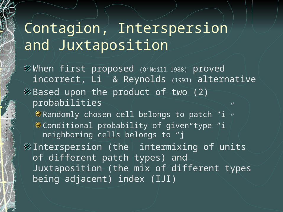
Contagion, Interspersion and Juxtaposition

When first proposed (O’Neill 1988) proved incorrect, Li & Reynolds (1993) alternativeBased upon the product of two (2) probabilities

Randomly chosen cell belongs to patch “i”Conditional probability of given type “i” neighboring cells belongs to “j”

Interspersion (the intermixing of units of different patch types) and Juxtaposition (the mix of different types being adjacent) index (IJI)

Changing patternsMonth NP LPI LSI MPFD IJI

January 21.00 28.46 7.79 1.35 66.89

February 98.00 25.08 9.64 1.27 65.57

March 92.25 21.61 9.65 1.29 67.23

April 93.73 18.99 8.43 1.26 70.12

May 84.00 25.45 9.04 1.29 68.67

June 103.33 15.00 9.39 1.27 71.96

July 82.86 25.03 9.38 1.29 70.63

August 24.10 26.23 7.96 1.33 72.40

September 20.78 26.78 7.96 1.34 70.18

October 22.08 25.78 7.97 1.35 65.60

November 20.80 29.94 7.95 1.37 67.21

December 21.43 32.32 7.57 1.34 67.23

Flying