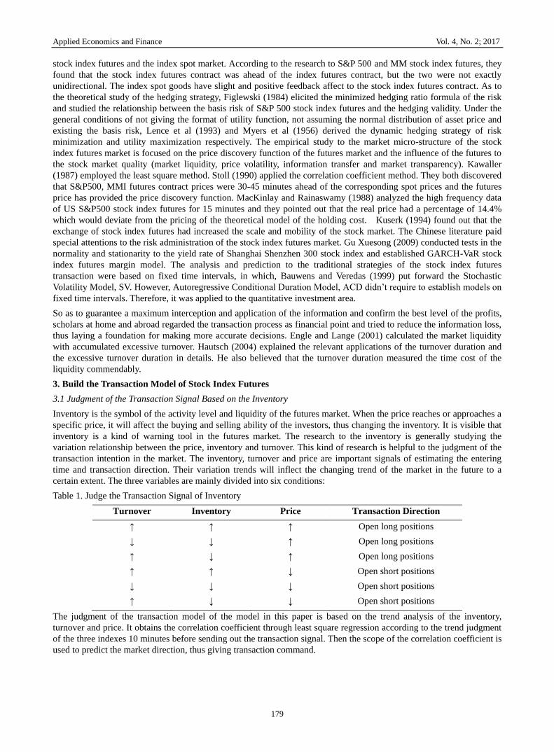
Applied Economics and Finance

Vol. 4, No. 2; March 2017

ISSN 2332-7294 E-ISSN 2332-7308

Published by Redfame Publishing

URL: http://aef.redfame.com

178

Research on Strategies of Stock Index Futures Transaction Based on

LMS Linear Regression Yaqian Pan1, Yang Li1, Shiqi Yu1, Xiaomin Fu1

1Finance Department of International Bussiness School, Jinan University, Zhuhai 519070, China;

Correspondence: Yaqian Pan, Finance Department of International Bussiness School, Jinan University, Qianshan road

206#, Zhuhai City, Guangdong Province, Post NO 519070, China.

Received: December 2, 2016 Accepted: December 22, 2016 Available online: February 16, 2017

doi:10.11114/aef.v4i2.2235 URL: https://dx.doi.org/10.11114/aef.v4i2.2235

Abstract

In recent years, stock index futures has developed into an important financial derivative in the global capital market and

provided an indispensable investment and hedging tool for investors. This paper is mainly studying the low frequency

transaction of stock index futures. Firstly, it conducts data cleaning to the stock index futures data and has an

interpolation calculation to the missing values. Afterwards, it judges the market information in the short period and

achieves the purpose of gaining profits through the basis. Furthermore, the time and the price difference are used as the

key factors for establishing the quantitative model of gaining profits. Through lease square regression and inventory

analysis technology, it completes the whole transaction process with several actions such as judging the open position

time, transaction direction, reverse position closing time and yield accounting. Finally, as to the regression testing of the

model, it detects the expression of the strategy through annual earnings, maximum drawback, transaction frequency,

Sharpe ratio, variety commonality and cycle commonality. In the end, it conducts scientific analysis to the approaches

used in the model and discusses the advantages and disadvantages of the model, thus providing some optimizing

strategies in considering the improvement direction in practical application.

Keywords: quantitative transactions, inventory analysis technique, lease square regression, regression testing of the

model

1. Research Background and Current Situation

Futures is the transaction agreement which conducts look-ahead buying and selling according to the firm price. The

futures trading is divided into speculation and delivery. Speculation means gaining price difference through buying low

and selling high or through selling high and buying low while delivery refers to the bargaining transaction which is

going to be carried out in the future at the fixed transaction price. Stock index futures is exactly the futures contract with

the stock price index as the subject matter. It has the effects as avoiding investment risk, interest arbitrage, reducing

stock market fluctuation rate and enriching the investment strategy. The achievement of the above functions of the stock

index futures is based on a mature market, in which the interaction of the spot price and the future price will bring the

variation of the transaction price.

Since the exchange of stock index futures has the characteristics of T+0 and the leveraged transaction of the cash

deposit, it has more risks than the exchange of the ordinary shares. China has pushed out the stock index futures in 2010.

During this period, Shanghai Shenzhen 300 index futures had an over 99% fitting degree with Shanghai Shenzhen 300

index. However, since the irregular development of the stock index futures market in China has brought risk-taking

mentalities to some investors, there are too many speculation factors in the market. Since December, 2014, the trading

volume of the stock index futures had a jumpy growth. From May, 2015 to August, 2015, the average daily trading

volume of Shanghai Shenzhen 300 stock index futures has surpassed 2500 billion. The abnormal upsurge had brought

hidden dangers to the great shock of the futures market in the later period. Since June, 15th, 2015, the stock index

futures and Shanghai Shenzhen 300 index have shown a great decline, with amplitude reaching almost 40%. Several

stock index futures have shown daily fluctuations of over 5% in high frequency. The great fluctuations are affected by

the market factors and its self risk amplification, which has brought the danger of market investment. Therefore, it is

extremely urgent to conduct risk control and administration to the stock index futures

2. Literature Review

As to the finding of the price function, Stoll and Whaley (1990) studies how the information is transmitted between the

Applied Economics and Finance Vol. 4, No. 2; 2017

179

stock index futures and the index spot market. According to the research to S&P 500 and MM stock index futures, they

found that the stock index futures contract was ahead of the index futures contract, but the two were not exactly

unidirectional. The index spot goods have slight and positive feedback affect to the stock index futures contract. As to

the theoretical study of the hedging strategy, Figlewski (1984) elicited the minimized hedging ratio formula of the risk

and studied the relationship between the basis risk of S&P 500 stock index futures and the hedging validity. Under the

general conditions of not giving the format of utility function, not assuming the normal distribution of asset price and

existing the basis risk, Lence et al (1993) and Myers et al (1956) derived the dynamic hedging strategy of risk

minimization and utility maximization respectively. The empirical study to the market micro-structure of the stock

index futures market is focused on the price discovery function of the futures market and the influence of the futures to

the stock market quality (market liquidity, price volatility, information transfer and market transparency). Kawaller

(1987) employed the least square method. Stoll (1990) applied the correlation coefficient method. They both discovered

that S&P500, MMI futures contract prices were 30-45 minutes ahead of the corresponding spot prices and the futures

price has provided the price discovery function. MacKinlay and Rainaswamy (1988) analyzed the high frequency data

of US S&P500 stock index futures for 15 minutes and they pointed out that the real price had a percentage of 14.4%

which would deviate from the pricing of the theoretical model of the holding cost. Kuserk (1994) found out that the

exchange of stock index futures had increased the scale and mobility of the stock market. The Chinese literature paid

special attentions to the risk administration of the stock index futures market. Gu Xuesong (2009) conducted tests in the

normality and stationarity to the yield rate of Shanghai Shenzhen 300 stock index and established GARCH-VaR stock

index futures margin model. The analysis and prediction to the traditional strategies of the stock index futures

transaction were based on fixed time intervals, in which, Bauwens and Veredas (1999) put forward the Stochastic

Volatility Model, SV. However, Autoregressive Conditional Duration Model, ACD didn’t require to establish models on

fixed time intervals. Therefore, it was applied to the quantitative investment area.

So as to guarantee a maximum interception and application of the information and confirm the best level of the profits,

scholars at home and abroad regarded the transaction process as financial point and tried to reduce the information loss,

thus laying a foundation for making more accurate decisions. Engle and Lange (2001) calculated the market liquidity

with accumulated excessive turnover. Hautsch (2004) explained the relevant applications of the turnover duration and

the excessive turnover duration in details. He also believed that the turnover duration measured the time cost of the

liquidity commendably.

3. Build the Transaction Model of Stock Index Futures

3.1 Judgment of the Transaction Signal Based on the Inventory

Inventory is the symbol of the activity level and liquidity of the futures market. When the price reaches or approaches a

specific price, it will affect the buying and selling ability of the investors, thus changing the inventory. It is visible that

inventory is a kind of warning tool in the futures market. The research to the inventory is generally studying the

variation relationship between the price, inventory and turnover. This kind of research is helpful to the judgment of the

transaction intention in the market. The inventory, turnover and price are important signals of estimating the entering

time and transaction direction. Their variation trends will inflect the changing trend of the market in the future to a

certain extent. The three variables are mainly divided into six conditions:

Table 1. Judge the Transaction Signal of Inventory

Turnover Inventory Price Transaction Direction

↑ ↑ ↑ Open long positions

↓ ↓ ↑ Open long positions

↑ ↓ ↑ Open long positions

↑ ↑ ↓ Open short positions

↓ ↓ ↓ Open short positions

↑ ↓ ↓ Open short positions

The judgment of the transaction model of the model in this paper is based on the trend analysis of the inventory,

turnover and price. It obtains the correlation coefficient through least square regression according to the trend judgment

of the three indexes 10 minutes before sending out the transaction signal. Then the scope of the correlation coefficient is

used to predict the market direction, thus giving transaction command.

Applied Economics and Finance Vol. 4, No. 2; 2017

180

4. Model Building

4.1 Data Pre-processing

Matlab data grasp algorithm is applied to get the K line data of 1 minute from Shanghai Shenzhen stock index futures

within three years. Then by treating and matching the time and K line data, it conducts data pre-cleaning, eliminates the

abnormal values and utilizes multiple interpolations to fill up the missing data of the suspension data.

4.2 Transaction Triggering Rules Based on Least Square Regression

The general quantitative strategy includes intraday strategy, trending strategy and mode recognition strategy. This paper

combines the intraday strategy and trending strategy and then acquires the regression coefficient of the transaction price

of T minutes before through lease square regression. Then the regression coefficient is regarded as the criteria of the

market tendency while the specific coefficient boundary is served as the entering signal. After that, the positive and

negative of the coefficient is treated to judge the transaction direction. If the coefficient is higher than 3, it is required to

open long positions. If the coefficient is lower than -2, it is required to open short positions. If the coefficient is between

-2 and 3, it is not required to open positions. After opening the positions, the algorithm will continue to search

transaction signal and buy in more shares to continue open short or long positions in the same direction. While setting

the triggering conditions of closing positions reversely, it combines target closing, secondary closing, and stop-loss

closing and sets three conditions of closing. For example, when it is opening the long positions, the target closing point

is 5% higher than the entry price; the secondary closing point is 0.5% lower than the maximum closing price and the

stop-loss closing point is 6% lower than the closing price. Finally, it is required to calculate the profits and losses of

every minute and accumulate. When the total revenue has lost 900000, stop investing and go bankrupt.

4.2.1 Detailed Algorithm of Transaction Triggering Rules

As to moment t1 (T<t1<242720 ), we firstly apply lease square regression to fit the relationship tendency slope a1,a2,a3

between the closing price, turnover, and inventory from moment t1 to T and moment t1 to 1. Then we can make the

following judgment.

{

a1≥A1，buy is real

a1≤A2，sell short is real

A2<a1<A1，do nothing

In which, T is the selected periodic coefficient to predict the tendency, which means that the current stock index

tendency is predicted according to the tendency in T minutes before, thus the judgment of opening long or short

positions will be made. A1, A2 are the parameters of predicting opening long or short positions. When a1 is higher than

A1, it is required to open long positions, otherwise, it is required to open short positions.

If buy or sellshort is true, mark t= t1, t2=t1 and turn to (2), otherwise carry out t1= t1 +1 and turn to (1).

1) Try to make t=t+1 and then compare a1 in moment t and t2.If the absolute value of the former a1 is bigger than the

absolute value of the latter, it is required to continue opening long or short positions (add one hand every time), make t2

=t and then turn to (2). If the absolute value of the former is less than or equal to the absolute value of the latter, make

t=t-1 and then carry out the next operation.

2) Make t=t+1 and maxprice=max{𝐻𝑖𝑔ℎ(𝑡1), … , 𝐻𝑖𝑔ℎ(𝑡 − 1)}, and it represents the top price which has ever appeared

in the current period. Make minprice=min{𝐿𝑜𝑤(𝑡1), … , 𝐿𝑜𝑤(𝑡 − 1)}, and it represents the minimum price which has

ever appeared in the current period. When buy is true, if it meets the conditions of 𝑚𝑎𝑥𝑝𝑟𝑖𝑐𝑒

𝑐𝑙𝑜𝑠𝑒(𝑡−1)− 1 ≥ 𝐵1 or 1 −

𝑐𝑙𝑜𝑠𝑒(𝑡1)

𝑐𝑙𝑜𝑠𝑒(𝑡−1)≥ 𝐵2 or close(t − 2) − close(t − 1) ≥ 𝐵3 ,sell can be predicted as true and turn to (1), otherwise repeat (3).

When the sellshort is true, if it reaches the conditions of 1 −𝑚𝑖𝑛𝑝𝑟𝑖𝑐𝑒

𝑐𝑙𝑜𝑠𝑒(𝑡−1)≥ 𝐶1 or

𝑐𝑙𝑜𝑠𝑒(𝑡1)

𝑐𝑙𝑜𝑠𝑒(𝑡−1)− 1 ≥ 𝐶2 or Close(t − 1) −

Close(t − 2) ≥ 𝐶3 ,buycover is judged as true. In which, B1, B2, B3, C1, C2 ,C3 are respectively the controllable

losses of closing long and short positions, estimated increase amount and judging criteria of emergency situations, it can

be set as 0.005,0.003, 10 for the time being.

3) The model can be improved through regulating the parameters A1 , A2, B1, B2, B3,C1, C2 ,C3 continually,

thus choosing a better solution.

Applied Economics and Finance Vol. 4, No. 2; 2017

181

4.2.2 The Calculating Means of the Total Profits (Index points)

1) If the operation of opening long positions is carried at the moment of t-1, the calculation of the profit in each

minute has to be added with the settled profit of the current minute, that is profit(t) = profit(t − 1) +

[𝐶𝑙𝑜𝑠𝑒(𝑡) − 𝐶𝑙𝑜𝑠𝑒(𝑡 − 1)] × (𝑡2 − 𝑡1 + 1)

2) If the operation of opening short positions is carried at the moment of t-1, the calculation of the profit in each

minute has to be added with the settled profit of the current minute, that is profit(t) = profit(t − 1) +

[−𝐶𝑙𝑜𝑠𝑒(𝑡) + 𝐶𝑙𝑜𝑠𝑒(𝑡 − 1)] × (𝑡2 − 𝑡1 + 1)

3) If the operation of closing positions is carried at the moment of t, then every profit has to be deducted the

handling charges. That is profit(t) = profit(t) − fee × Close(t) × (𝑡2 − 𝑡1 + 1)

4) If the operation of opening positions is carried at the moment of t, then every profit has to be deducted the

handling charges. That is profit(t) = profit(t) − fee × Close(t) . When profit(t) < −3000 , shut down

procedure, and put out t.

4.2.3 Simulation Operation Analysis of the Model

Firstly, it is required to choose the proper prediction time from the perspective of maximizing the profit. After

tests, T value is better to be around 20. We make the tendency slope between the closing price and time with T

value set at 10,17,20,25,30 within 12351-12360 minutes and 210325-210334 minutes. Therefore, we make the

following Table 2.

Table 2. The comparative statement of the tendency slope with different T

T 12351 12352 12353 12354 12355 12356 12357 12358 12359 12360

10 -2.50 -2.49 -2.13 -1.50 -0.53 0.40 0.57 0.61 0.49 0.12

17 -1.11 -1.28 -1.32 -1.32 -1.34 -1.25 -1.11 -0.96 -0.79 -0.69

20 -0.76 -0.93 -1.00 -1.03 -1.07 -1.06 -1.05 -1.02 -0.92 -0.86

25 -0.40 -0.51 -0.57 -0.62 -0.69 -0.74 -0.78 -0.79 -0.78 -0.82

30 -0.39 -0.41 -0.41 -0.39 -0.45 -0.49 -0.52 -0.54 -0.56 -0.62

T 210325 210326 210327 210328 210329 210330 210331 210332 210333 210334

10 -6.31 -6.64 -6.52 -5.76 -4.45 -2.73 -0.23 0.61 0.33 0.27

17 -2.71 -3.18 -3.54 -3.76 -3.87 -3.89 -3.73 -3.45 -3.15 -2.73

20 -2.09 -2.45 -2.75 -2.97 -3.14 -3.26 -3.26 -3.19 -3.10 -2.94

25 -1.39 -1.66 -1.91 -2.11 -2.29 -2.43 -2.50 -2.53 -2.56 -2.57

30 -0.96 -1.16 -1.36 -1.54 -1.69 -1.84 -1.92 -1.99 -2.06 -2.12

Combining the variation tendency of the practical closing price, we get to know that the tendency slope has a smart

variation with the fluctuation of the closing price and it is disjointed with the current closing price when T=10.

Therefore, it is not good for predicting the tendency of the current closing price. When T=30, the tendency slope has a

gentle variation with the fluctuation of the closing price and it is not good for seizing opportunities, thus it is not

profitable. Hence, T value is better to be around 20.

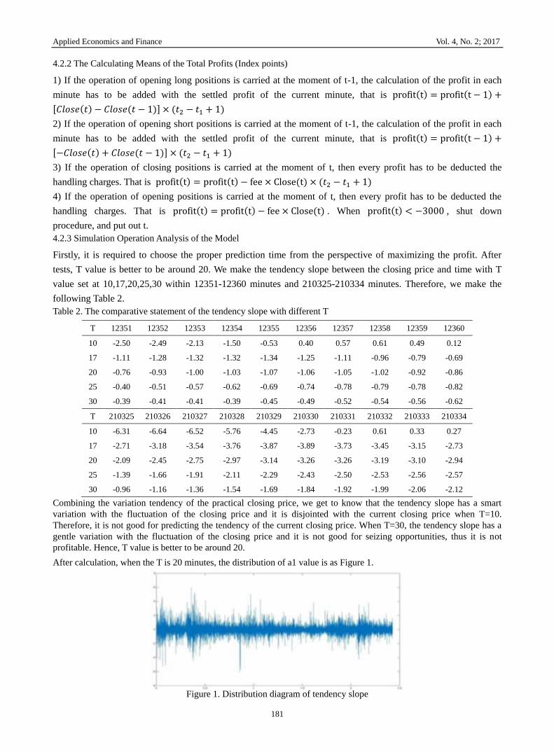
After calculation, when the T is 20 minutes, the distribution of a1 value is as Figure 1.

Figure 1. Distribution diagram of tendency slope

Applied Economics and Finance Vol. 4, No. 2; 2017

182

From the diagram, we can conclude that there is little frequency out of the scope. Then the selection ranges of A1 , A2

are [0,4] and [0, −4] respectively. Combining the expert opinions and the practical conditions, it can be A1=3 and

A2=2 for the time being.

However, B1 , B2, B3, C1, C2, C3 are the estimated losses of closing long positions and short positions, estimated

increase amount and the determination coefficient of emergent situation respectively. The determination of the six

parameters is related to the psychology of the investors. If the investor is risky, he can turn up the estimated increase

amount of closing the long and short positions, estimated losses as well as the determination coefficient of emergent

situation (stop value) properly. Otherwise, he can minish the parameters properly. The scope of the six parameters

chosen in this paper is as the following. 𝐵1 ∈ [0.005,0.01] ,𝐵2 ∈ [0.005,0.05] ,𝐵3 ∈ [3,20] ,𝐶1 ∈ [0.005,0.01] ,𝐶2 ∈[0.005,0.05] ,𝐶3 ∈ [3,20] .

The actual income of t moment is the total revenue of t moment (index points) multiply by 300.

Sumprofit(t) = profit(t) × 300

The final profit is exactly the profit of t=242720.

finalprofit = Sumprofit(242720)

The price trend of the preceding 17 minutes will be obtained through least square regression. Then the signal of opening

positions can be searched.

From the above statements, we can find out that there are three conditions to close the short positions:

1 −𝑚𝑖𝑛𝑝𝑟𝑖𝑐𝑒

𝑐𝑙𝑜𝑠𝑒(𝑡−1)≥ 𝐶1 or

𝑐𝑙𝑜𝑠𝑒(𝑡1)

𝑐𝑙𝑜𝑠𝑒(𝑡−1)− 1 ≥ 𝐶2 or Close(t − 1) − Close(t − 2) ≥ 𝐶3 .As to T=213405, minprice

=2229.6, Close(t1)=2233.6, Close(t-1)=2236.2, Close(t-2)=2230.2, set C1, C2, C3 at 0.01,0.08,25 respectively,

and the results of the three conditions of closing positions are as following:

1 −𝑚𝑖𝑛𝑝𝑟𝑖𝑐𝑒

𝐶𝑙𝑜𝑠𝑒(𝑡−1)= 1 −

2229.6

2236.2= 0.003 < 𝐶1 ,

𝐶𝑙𝑜𝑠𝑒(𝑡1)

𝐶𝑙𝑜𝑠𝑒(𝑡−1)− 1 =

2233.6

2236.2− 1 = 0.001 < 𝐶2 , Close(t − 1) − Close(t −

2) = 2236.2 − 2230.2 = 6 < 𝐶3 .The three conditions are not satisfied. So, it will not close the positions and

then jump to the next moment to repeat the same judgment.

After calculation, when T jumps to 213419, the condition of closing the positions is reached (1 −𝑚𝑖𝑛𝑝𝑟𝑖𝑐𝑒

𝐶𝑙𝑜𝑠𝑒(𝑡−1)= 1 −

2229.6

2257.2= 0.012 > 𝐶1). Therefore, the closing position operation is made at this moment. And then it continues to

judge if it will go on opening long or short positions. And so on, the operation of opening or closing long positions

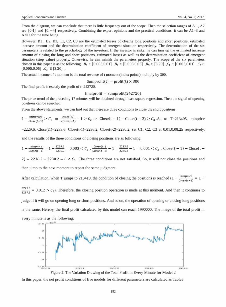
is the same. Hereby, the final profit calculated by this model can reach 1990000. The image of the total profit in

every minute is as the following:

Figure 2. The Variation Drawing of the Total Profit in Every Minute for Model 2

In this paper, the net profit conditions of five models for different parameters are calculated as Table3.

Applied Economics and Finance Vol. 4, No. 2; 2017

183

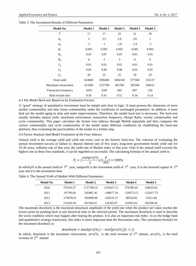
Table 3. The Investment Results of Different Parameters

Model No. Model 1 Model 2 Model 3 Model 4 Model 5

T 17 17 20 21 30

A1 3 2.5 2.8 2.8 3

A2 -2 -1 -1.8 -1.9 -2

B1 0.005 0.005 0.005 0.005 0.005

B2 0.05 0.07 0.05 0.05 0.05

B3 6 3 3 6 6

C1 0.01 0.01 0.01 0.01 0.01

C2 0.05 0.08 0.08 0.05 0.05

C3 20 25 25 20 20

Final yield 634600 1990400 1004100 577560 235137

Maximum retracement 411000 1127700 462700 395500 394521

Transaction frequency 1029 3549 843 807 228

Risk-reward ratio 0.36 0.41 0.51 0.34 0.14

4.3 The Model Back-test Based on Its Evaluation Factors

A “good” strategy of quantitative investment must be simple and clear in logic. It must possess the characters of more

market commonality and time frame commonality under the conditions of unchanged parameters. In addition, it must

find out the model aging in time and make improvements. Therefore, the model back-test is necessary. The back-test

usually includes annual yield, maximum retracement, transaction frequency, Sharpe Ratio, variety commonality and

cycle commonality. This paper calculates the former four indexes through Matlab separately and then compares the

variety commonality and cycle commonality of the model under different conditions by establishing the back-test

platform, thus evaluating the practicability of the model in a further step.

4.4 Factor Analysis And Model Evaluation of the Four Indexes

Annual yield is the average yield and yield rate every year in the historic back-test. The criterion of evaluating the

annual investment success or failure is: deposit interest rate of five years, long-term government bonds yield rate for

10-30 years, inflation rate of that year, the yield rate of Market index of that year. Only if the annual yield exceeds the

highest one in these four standards, it can be regarded as successful. The calculating formula of the annual yield is:

𝑃𝑖 = (𝑠𝑢𝑚𝑝𝑟𝑜𝑓𝑖𝑡

𝐼𝑖)/(

𝑑

365) × 100%

In which,Pi is the annual yield of i𝑡ℎ year, sumprofit is the investment yield of i𝑡ℎ year, Ii is the invested capital of i𝑡ℎ

year and d is the investment date.

Table 4. The Annual Yield of Models With Different Parameters

Model No. Model 1 Model 2 Model 3 Model 4 Model 5

2010 755193.57 1717299.35 1191827.12 576788.30 239635.03

2011 -81700.64 245481.36 -148677.34 -129273.15 -125417.73

2012 -174078.91 -563909.96 -165233.27 -80516.65 15521.08

2013 135183.29 591569.61 126205.07 210563.02 105398.34

The maximum drawback is the maximum drawback amplitude of the yield rate when the product net value reaches the

lowest point by pushing back at any historical time in the selected period. The maximum drawback is used to describe

the worst condition which may happen after buying the product. It is also an important risk index. As to the hedge fund

and quantitative strategy transaction, this index is more important than the fluctuation ratio. The calculation formula for

the maximum drawback is:

drawback = max{𝑝𝑟𝑜𝑓𝑖𝑡𝑖} − 𝑚𝑖𝑛{𝑝𝑟𝑜𝑓𝑖𝑡𝑗}(𝑖 < 𝑗)

In which, drawback is the maximum retracement, 𝑝𝑟𝑜𝑓𝑖𝑡𝑖 is the total revenue of i𝑡ℎ minute, 𝑝𝑟𝑜𝑓𝑖𝑡𝑗 is the total

revenue of j𝑡ℎ minute

Applied Economics and Finance Vol. 4, No. 2; 2017

184

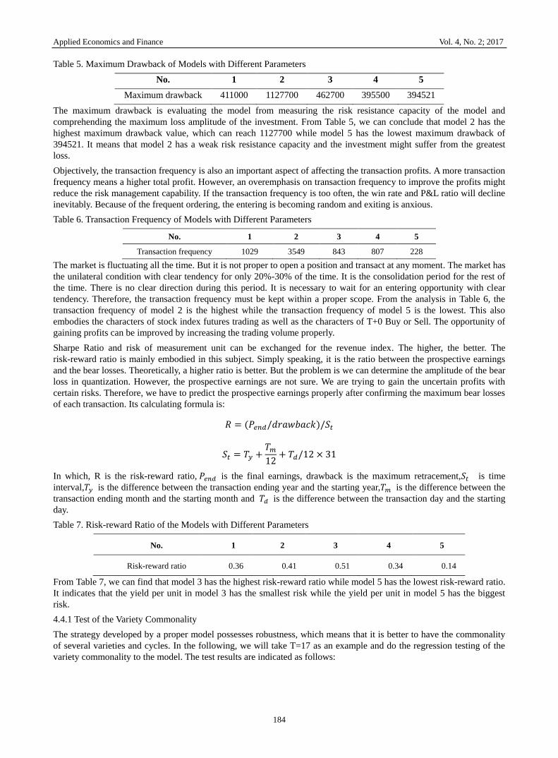
Table 5. Maximum Drawback of Models with Different Parameters

No. 1 2 3 4 5

Maximum drawback 411000 1127700 462700 395500 394521

The maximum drawback is evaluating the model from measuring the risk resistance capacity of the model and

comprehending the maximum loss amplitude of the investment. From Table 5, we can conclude that model 2 has the

highest maximum drawback value, which can reach 1127700 while model 5 has the lowest maximum drawback of

394521. It means that model 2 has a weak risk resistance capacity and the investment might suffer from the greatest

loss.

Objectively, the transaction frequency is also an important aspect of affecting the transaction profits. A more transaction

frequency means a higher total profit. However, an overemphasis on transaction frequency to improve the profits might

reduce the risk management capability. If the transaction frequency is too often, the win rate and P&L ratio will decline

inevitably. Because of the frequent ordering, the entering is becoming random and exiting is anxious.

Table 6. Transaction Frequency of Models with Different Parameters

No. 1 2 3 4 5

Transaction frequency 1029 3549 843 807 228

The market is fluctuating all the time. But it is not proper to open a position and transact at any moment. The market has

the unilateral condition with clear tendency for only 20%-30% of the time. It is the consolidation period for the rest of

the time. There is no clear direction during this period. It is necessary to wait for an entering opportunity with clear

tendency. Therefore, the transaction frequency must be kept within a proper scope. From the analysis in Table 6, the

transaction frequency of model 2 is the highest while the transaction frequency of model 5 is the lowest. This also

embodies the characters of stock index futures trading as well as the characters of T+0 Buy or Sell. The opportunity of

gaining profits can be improved by increasing the trading volume properly.

Sharpe Ratio and risk of measurement unit can be exchanged for the revenue index. The higher, the better. The

risk-reward ratio is mainly embodied in this subject. Simply speaking, it is the ratio between the prospective earnings

and the bear losses. Theoretically, a higher ratio is better. But the problem is we can determine the amplitude of the bear

loss in quantization. However, the prospective earnings are not sure. We are trying to gain the uncertain profits with

certain risks. Therefore, we have to predict the prospective earnings properly after confirming the maximum bear losses

of each transaction. Its calculating formula is:

𝑅 = (𝑃𝑒𝑛𝑑/𝑑𝑟𝑎𝑤𝑏𝑎𝑐𝑘)/𝑆𝑡

𝑆𝑡 = 𝑇𝑦 +𝑇𝑚

12+ 𝑇𝑑/12 × 31

In which, R is the risk-reward ratio, 𝑃𝑒𝑛𝑑 is the final earnings, drawback is the maximum retracement,𝑆𝑡 is time

interval,𝑇𝑦 is the difference between the transaction ending year and the starting year,𝑇𝑚 is the difference between the

transaction ending month and the starting month and 𝑇𝑑 is the difference between the transaction day and the starting

day.

Table 7. Risk-reward Ratio of the Models with Different Parameters

No. 1 2 3 4 5

Risk-reward ratio 0.36 0.41 0.51 0.34 0.14

From Table 7, we can find that model 3 has the highest risk-reward ratio while model 5 has the lowest risk-reward ratio.

It indicates that the yield per unit in model 3 has the smallest risk while the yield per unit in model 5 has the biggest

risk.

4.4.1 Test of the Variety Commonality

The strategy developed by a proper model possesses robustness, which means that it is better to have the commonality

of several varieties and cycles. In the following, we will take T=17 as an example and do the regression testing of the

variety commonality to the model. The test results are indicated as follows:

Applied Economics and Finance Vol. 4, No. 2; 2017

185

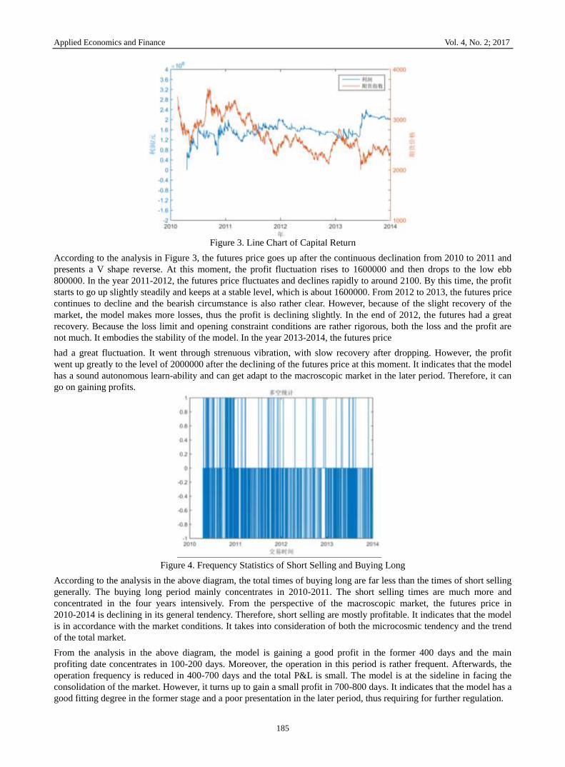
Figure 3. Line Chart of Capital Return

According to the analysis in Figure 3, the futures price goes up after the continuous declination from 2010 to 2011 and

presents a V shape reverse. At this moment, the profit fluctuation rises to 1600000 and then drops to the low ebb

800000. In the year 2011-2012, the futures price fluctuates and declines rapidly to around 2100. By this time, the profit

starts to go up slightly steadily and keeps at a stable level, which is about 1600000. From 2012 to 2013, the futures price

continues to decline and the bearish circumstance is also rather clear. However, because of the slight recovery of the

market, the model makes more losses, thus the profit is declining slightly. In the end of 2012, the futures had a great

recovery. Because the loss limit and opening constraint conditions are rather rigorous, both the loss and the profit are

not much. It embodies the stability of the model. In the year 2013-2014, the futures price

had a great fluctuation. It went through strenuous vibration, with slow recovery after dropping. However, the profit

went up greatly to the level of 2000000 after the declining of the futures price at this moment. It indicates that the model

has a sound autonomous learn-ability and can get adapt to the macroscopic market in the later period. Therefore, it can

go on gaining profits.

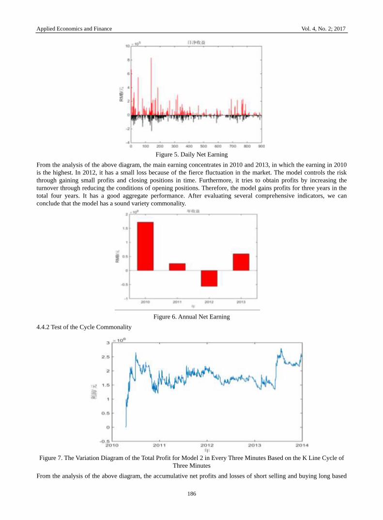
Figure 4. Frequency Statistics of Short Selling and Buying Long

According to the analysis in the above diagram, the total times of buying long are far less than the times of short selling

generally. The buying long period mainly concentrates in 2010-2011. The short selling times are much more and

concentrated in the four years intensively. From the perspective of the macroscopic market, the futures price in

2010-2014 is declining in its general tendency. Therefore, short selling are mostly profitable. It indicates that the model

is in accordance with the market conditions. It takes into consideration of both the microcosmic tendency and the trend

of the total market.

From the analysis in the above diagram, the model is gaining a good profit in the former 400 days and the main

profiting date concentrates in 100-200 days. Moreover, the operation in this period is rather frequent. Afterwards, the

operation frequency is reduced in 400-700 days and the total P&L is small. The model is at the sideline in facing the

consolidation of the market. However, it turns up to gain a small profit in 700-800 days. It indicates that the model has a

good fitting degree in the former stage and a poor presentation in the later period, thus requiring for further regulation.

Applied Economics and Finance Vol. 4, No. 2; 2017

186

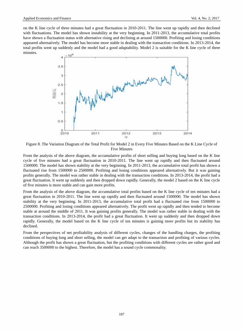
Figure 5. Daily Net Earning

From the analysis of the above diagram, the main earning concentrates in 2010 and 2013, in which the earning in 2010

is the highest. In 2012, it has a small loss because of the fierce fluctuation in the market. The model controls the risk

through gaining small profits and closing positions in time. Furthermore, it tries to obtain profits by increasing the

turnover through reducing the conditions of opening positions. Therefore, the model gains profits for three years in the

total four years. It has a good aggregate performance. After evaluating several comprehensive indicators, we can

conclude that the model has a sound variety commonality.

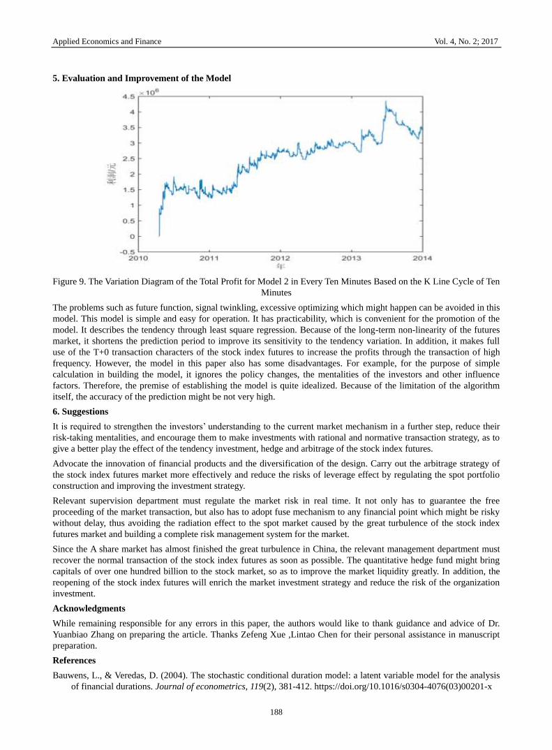
Figure 6. Annual Net Earning

4.4.2 Test of the Cycle Commonality

Figure 7. The Variation Diagram of the Total Profit for Model 2 in Every Three Minutes Based on the K Line Cycle of

Three Minutes

From the analysis of the above diagram, the accumulative net profits and losses of short selling and buying long based

Applied Economics and Finance Vol. 4, No. 2; 2017

187

on the K line cycle of three minutes had a great fluctuation in 2010-2011. The line went up rapidly and then declined

with fluctuations. The model has shown instability at the very beginning. In 2011-2013, the accumulative total profits

have shown a fluctuation status with alternative rising and declining at around 1500000. Profiting and losing conditions

appeared alternatively. The model has become more stable in dealing with the transaction conditions. In 2013-2014, the

total profits went up suddenly and the model had a good adaptability. Model 2 is suitable for the K line cycle of three

minutes.

Figure 8. The Variation Diagram of the Total Profit for Model 2 in Every Five Minutes Based on the K Line Cycle of

Five Minutes

From the analysis of the above diagram, the accumulative profits of short selling and buying long based on the K line

cycle of five minutes had a great fluctuation in 2010-2011. The line went up rapidly and then fluctuated around

1500000. The model has shown stability at the very beginning. In 2011-2013, the accumulative total profit has shown a

fluctuated rise from 1500000 to 2500000. Profiting and losing conditions appeared alternatively. But it was gaining

profits generally. The model was rather stable in dealing with the transaction conditions. In 2013-2014, the profit had a

great fluctuation. It went up suddenly and then dropped down rapidly. Generally, the model 2 based on the K line cycle

of five minutes is more stable and can gain more profits.

From the analysis of the above diagram, the accumulative total profits based on the K line cycle of ten minutes had a

great fluctuation in 2010-2011. The line went up rapidly and then fluctuated around 1500000. The model has shown

stability at the very beginning. In 2011-2013, the accumulative total profit had a fluctuated rise from 1500000 to

2500000. Profiting and losing conditions appeared alternatively. The profit went up rapidly and then tended to become

stable at around the middle of 2011. It was gaining profits generally. The model was rather stable in dealing with the

transaction conditions. In 2013-2014, the profit had a great fluctuation. It went up suddenly and then dropped down

rapidly. Generally, the model based on the K line cycle of ten minutes is gaining more profits but its stability has

declined.

From the perspectives of net profitability analysis of different cycles, changes of the handling charges, the profiting

conditions of buying long and short selling, the model can get adapt to the transaction and profiting of various cycles.

Although the profit has shown a great fluctuation, but the profiting conditions with different cycles are rather good and

can reach 3500000 to the highest. Therefore, the model has a sound cycle commonality.

Applied Economics and Finance Vol. 4, No. 2; 2017

188

5. Evaluation and Improvement of the Model

Figure 9. The Variation Diagram of the Total Profit for Model 2 in Every Ten Minutes Based on the K Line Cycle of Ten

Minutes

The problems such as future function, signal twinkling, excessive optimizing which might happen can be avoided in this

model. This model is simple and easy for operation. It has practicability, which is convenient for the promotion of the

model. It describes the tendency through least square regression. Because of the long-term non-linearity of the futures

market, it shortens the prediction period to improve its sensitivity to the tendency variation. In addition, it makes full

use of the T+0 transaction characters of the stock index futures to increase the profits through the transaction of high

frequency. However, the model in this paper also has some disadvantages. For example, for the purpose of simple

calculation in building the model, it ignores the policy changes, the mentalities of the investors and other influence

factors. Therefore, the premise of establishing the model is quite idealized. Because of the limitation of the algorithm

itself, the accuracy of the prediction might be not very high.

6. Suggestions

It is required to strengthen the investors’ understanding to the current market mechanism in a further step, reduce their

risk-taking mentalities, and encourage them to make investments with rational and normative transaction strategy, as to

give a better play the effect of the tendency investment, hedge and arbitrage of the stock index futures.

Advocate the innovation of financial products and the diversification of the design. Carry out the arbitrage strategy of

the stock index futures market more effectively and reduce the risks of leverage effect by regulating the spot portfolio

construction and improving the investment strategy.

Relevant supervision department must regulate the market risk in real time. It not only has to guarantee the free

proceeding of the market transaction, but also has to adopt fuse mechanism to any financial point which might be risky

without delay, thus avoiding the radiation effect to the spot market caused by the great turbulence of the stock index

futures market and building a complete risk management system for the market.

Since the A share market has almost finished the great turbulence in China, the relevant management department must

recover the normal transaction of the stock index futures as soon as possible. The quantitative hedge fund might bring

capitals of over one hundred billion to the stock market, so as to improve the market liquidity greatly. In addition, the

reopening of the stock index futures will enrich the market investment strategy and reduce the risk of the organization

investment.

Acknowledgments

While remaining responsible for any errors in this paper, the authors would like to thank guidance and advice of Dr.

Yuanbiao Zhang on preparing the article. Thanks Zefeng Xue ,Lintao Chen for their personal assistance in manuscript

preparation.

References

Bauwens, L., & Veredas, D. (2004). The stochastic conditional duration model: a latent variable model for the analysis

of financial durations. Journal of econometrics, 119(2), 381-412. https://doi.org/10.1016/s0304-4076(03)00201-x

Applied Economics and Finance Vol. 4, No. 2; 2017

189

Cornell, B., & French, K. R. (1983). Taxes and the pricing of stock index futures. The Journal of Finance, 38(3),

675-694. https://doi.org/10.1111/j.1540-6261.1983.tb02496.x

Dong, F. (2015). On the Application of Fusing Mechanism in China's Stock Index Futures. Modern Business, 27,

112-113. http://dx.doi:10.3969/j.issn.1673-5889.2015.27.061

Figlewski, S. (1984). Hedging Performance and Basis Risk in Stock Index Futures. Journal of Finance, 39(3), 657-669.

https://doi.org/10.1111/j.1540-6261.1984.tb03654.x

Glosten, L. R., & Milgrom, P. R. (1985). Bid, ask and transaction prices in a specialist market with heterogeneously

informed traders. Journal of financial economics, 14(1), 71-100. https://doi.org/10.1016/0304-405x(85)90044-3

Kawaller, I, G., Koch, P, D., & Koch, T. W. (1987). The temporal price relationship between S&P 500 futures and the

S&P 500 index. Journal of Finance, 42(5), 1309- 1329. https://doi.org/10.1111/j.1540-6261.1987.tb04368.x

Kuserk, G. J., & Locke, P. R. (1994). Market maker competition on futures exchanges. The Journal of Derivatives, 1(4),

56-66. https://doi.org/10.3905/jod.1994.407894

Li, Y. Q. (2012). A Study on the Effect of Stock Index Futures on Short-term Market Volatility-Based on the Shanghai

and Shenzhen 300 stock index futures data. Friends of Accounting, 14, 99-12.

http://dx.doi:10.3969/j.issn.1004-5937.2012.14.034

Liang, X. Y. (2010). Research on Investment Strategy Simulation of Stock Index Futures Market Based on

Netlogo(Doctoral dissertation, Tianjin University).

Liu, B. (2008). An Empirical Analysis of Stock Index Futures Hedging Performance. (Doctoral dissertation, Tianjin

University).

Liu, X. C., & Chen, L. N. (2009). Research Progress, Method and Prospect of Stock Index Futures at Home and Abroad.

Academics in China, 6, 278-285.

Myers, R., Hanson, S. D. (1996). Optimal Dynamic Hedging in Unbiased Futures Markets. American Journal of

Agricultural Economics, 78(1), 13-13.https://doi.org/10.2307/1243774

Parlour, C. A. (1998). Price dynamics in limit order markets. Review of Financial Studies, 11(4), 789-816.

https://doi.org/10.1093/rfs/11.4.789

Stoll, H. R., & Whaley, R. E. (1990). The Dynamic of Stock Index and Stock Futures Return. The Journal of Financial

and Quantitative Analysis, 25(4), 441-468. https://doi.org/10.2307/2331010

Wang, X., & Yu, W. H. (2016). Research on Stock Index Futures Trading Strategy - Based on Autoregressive

Conditional Duration Model. Review of Investment Studies, 1, 122-136.

Wu, G. H. (2009). Simulation and Study on Trading Strategies of Stock Index Futures. (Doctoral dissertation, Tianjin

University).

Zhang, Y. K., & Yang, H. (2014). Pricing of Shanghai and Shenzhen Stock Index Futures Based on Black-Scholes

Model. Journal of Beihua University(Social Sciences), 15(2), 45-49.

http://dx.doi:10.3969/j.issn.1009-5101.2014.02.009

Copyrights

Copyright for this article is retained by the author(s), with first publication rights granted to the journal.

This is an open-access article distributed under the terms and conditions of the Creative Commons Attribution license

which permits unrestricted use, distribution, and reproduction in any medium, provided the original work is properly

cited.