APPLIED DYNAMICS - download.e-bookshelf.de · APPLIED DYNAMICS With Applications to Multibody and...

APPLIED DYNAMICS

With Applications to Multibody and Mechatronic Systems

FRANCIS C. MOON Cornell University

A Wiley-Interscience Publication

JOHN WILEY & SONS, INC. New York - Chichester - Weinheim . Brisbane - Singapore Toronto

APPLIED DYNAMICS

APPLIED DYNAMICS

With Applications to Multibody and Mechatronic Systems

FRANCIS C. MOON Cornell University

A Wiley-Interscience Publication

JOHN WILEY & SONS, INC. New York - Chichester - Weinheim . Brisbane - Singapore Toronto

This book is printed on acid-free paper.@

Copyright 0 1998 by John Wiley & Sons, Inc.

All rights reserved. Published simultaneously in Canada.

No part of this publication may be reproduced, stored in a retrieval system or transmitted in any form or by any means, electronic, mechanical, photocopying, recording, scanning or otherwise, except as permitted under Section 107 or 108 of the 1976 United States Copyright Act, without either the prior written permission of the Publisher, or authorization through payment of the appropriate per-copy fee to the Copyright Clearance Center, 222 Rosewood Drive, Danvers, MA 01923, (978) 750-8400, fax (978) 750-4744. Requests to the Publisher for permission should be addressed to the Permissions Department, John Wiley & Sons, Inc., 605 Third Avenue, New York, NY 10158-0012, (212) 850-601 1, fax (212) 850-6008, E-Mail: [email protected].

Library of Congress Cataloging-in-Publication Data

Moon, F. C., 1939- Applied dynamics : with applications to multibody and mechatronic

systems / by Francis C. Moon.

p. cm. “A Wiley-Interscience publication.” Includes bibliographical references (p. ISBN 0-471-13828-2 (cloth : alk. paper) 1. Dynamics. I. Title.

QA845.M657 1998 620.1 ’054--dc21

Printed in the United States of America

10 9 8 7 6 5 4 3

) and index.

97-20250 CIP

CONTENTS

Preface

1 Dynamic Phenomena and Failures

1.1 Introduction, 1

1.2 What’s New in Dynamics? 2

1.3 Dynamic Failures, 13

1.4 Basic Paradigms in Dynamics, 19

1.5 Coupled and Complex Dynamic Phenomena, 3 1

1.6 Dynamics and Design, 32

1.7 Modern Physics of Dynamics and Gravity, 33

2 Basic Principles of Dynamics

2.1 Introduction, 36

2.2 Kinematics, 36

2.3 Equilibrium and Virtual Work, 42

2.4 Systems of Particles, 44

2.5 Rigid Bodies, 51

2.6 D’Alembert’s Principle, 54

2.7 The Principle of Virtual Power, 56

ix

1

36

V

vi CONTENTS

62 3 Kinematics


3.2 Angular Velocity, 64

3.3 Matrix Representation of Angular Velocity, 67

3.4 Kinematics Relative to Moving Coordinate Frames, 68

3.5 Constraints and Jacobians, 72

3.6 Finite Motions, 75

3.7 Transformation Matrices for General Rigid-body Motion, 83

3.8 Kinematic Mechanisms, 88

4 Principles of D’Alembert, Virtual Power, and Lagrange’s Equations 103


4.2 D’Alembert’s Principle, 107

4.3 Lagrange’s Equations, 1 16

4.4 The Method of Virtual Power, 133

4.5 Nonholonomic Constraints: Lagrange Multipliers, 146

4.6 Variational Principles in Dynamics: Hamilton’s Principle, 153

5 Rigid Body Dynamics 168


5.2 Kinematics of Rigid Bodies, 171

5.3 Newton-Euler Equations of Motion, 181

5.4 Lagrange’s Equations for a Rigid Body, 205

5.5 Principle of Virtual Power for a Rigid Body, 214

5.6 Nonholonomic Rigid Body Problems, 230

6 Introduction to Robotics and Multibody Dynamics


6.2 Graph Theory and Incidence Matrices, 258

6.3 Kinematics, 265

6.4 Equations of Motion, 269

254

CONTENTS vii

6.5 Inverse Problems, 289

6.6 Impact Problems, 296

7 Orbital and Satellite Dynamics


7.2 Central-force Dynamics, 327

7.3 Two-body Problems, 338

7.4 Rigid-body Satellite Dynamics, 341

7.5 Tethered Satellites, 358

325

8 Electromechanical Dynamics: An Introduction to Mechatronics 374

8.1 Introduction and Applications, 374

8.2 Electric and Magnetic Forces, 376

8.3 Electromechanical Material Properties, 383

8.4 Dynamic Principles of Electromagnetics, 390

8.5 Lagrange’s Equations for Magnetic Systems, 395

8.6 Applications, 407

8.7 Control Dynamics, 416

9 Introduction to Nonlinear and Chaotic Dynamics


9.2 Nonlinear Resonance, 435

9.3 The Undampled Pendulum: Phase-plane Motions, 439

9.4 Self-excited Oscillations: Limit Cycles, 443

9.5 Flows and Maps: PoincarC Sections, 446

9.6 Complex Dynamics in Rigid-body Applications, 458

432

Appendix A Second Moments of Mass for Selected Geometric

Appendix B Commercial Dynamic Analysis and Simulation Software Codes 478

References 483

Index 487

Objects 474

PREFACE

The modern post industrial era has ushered in a new set of dynamics problems and applications, such as robotic systems, high-speed maneuver- able aircraft, microelectromechanical systems, space-craft dynamics, magnetic bearings, active suspension in automobiles, and 500-kph magnetically levitated trains. Up until the 1950s, engineers generally dealt with dynamic effects in machines and structures from a quasi-static point of view or not at all. In the last quarter of this century, however, incorporation of dynamic forces in design has become necessary, as new materials have permitted higher loads, speeds, and temperatures, resulting in more lightweight and optimally designed dynamical devices.

One success of the computer revolution in the field of dynamics has been the codification of analysis tools in linear dynamical systems. Codes are now available to accurately predict natural frequencies and mode shapes of complicated structures and machines. This has pushed the frontiers of dynamical analysis into nonlinear dynamics and multibody systems, and coupled field dynamical problems such as electromagneto-dynamics, fluid- structural dynamics, and intelligent control of machine-structure interactions. In Europe and Japan the combined field of dynamics, control, and computer science is called Mechatronics.

So why another textbook in dynamics? This book is written to fill a gap between elementary dynamics textbooks taught at the sophomore level, such as Meriam, Beers, Johnson, etc., and advanced theoretical books, such as Goldstein, Guckenheimer, and Holmes, etc., taught at the advanced graduate level. The focus of this book is on modern applied problems and new tools for analysis.

ix

X PREFACE

The goals of this textbook are:

0 To illustrate the phenomena and applications of modern dynamics through interesting examples without excessive mathematical abstrac- tion.

0 To introduce the student to a clear statement of the principles of dynamics in the context of modern analytical and computational methods.

0 To introduce modern methods of virtual velocities or principle of virtual power as developed by Jourdain, Kane, and others through clear illustrative examples.

0 To develop educated intuition about advanced dynamics phenomena. 0 To integrate modeling, derivation of equations, and solution of equa-

tions as much as possible. 0 To provide an introduction to applications related to robotics, mecha-

tronics, aerospace dynamics, multibody machine dynamics, and nonlinear dynamics.

The level chosen for this text is at the undergraduate senior, masters degree, or first-year graduate level, although an honors junior class should have no difficulty with the material.

Most parts of this book have been used in an Intermediate Dynamics course taught at Cornell University by the author over the course of a decade. Students who have taken the course have included mechanical and civil engineers, theoretical mechanics, and applied physics students. The levels have ranged from seniors, master of engineering, to Ph.D.-level students. The core of the material (Chapters 2-6) can be taught in a one-semester course or in two quarter-system courses. In recent years the author has taught the course using MATLAB and MATHEMATICA. Students are asked to write programs to automatically derive Lagrange’s equations or to obtain a time history of the motion. Also term projects have been used to teach the course in which students have 4-5 weeks to analyze and write a report about a specific dynamics application, often using the class notes as a launching platform to venture into more advanced material as given in the list of references and advanced texts.

Both vector and matrix methods are presented in the book. Experience has shown that students easily master Lagrange’s equations, but still struggle with the three-dimensional vector dynamics introduced in elementary courses in dynamics. Thus the author has kept a strong element of kinematics in the book.

An important feature of this book is the development of the method of virtual velocities based on the principle of virtual power. Virtual power ideas go back many centuries, but were formalized in dynamics by Jourdain at the turn of this century. In the 1960s Professor Thomas Kane of Stanford University developed a related formalism to derive equations of motion

PREFACE xi

using virtual velocities. However, in Europe and Germany a less formal, more direct use of the principle of virtual power has been used in textbooks and software. ‘This book presents the less formal approach. The method is not only simpler in many cases than Lagrange’s equations, but is sometimes more suited to solving multibody problems using computer methods.

The second half of the book reflects the author’s research interests, especially in magnetomechanical dynamics and nonlinear phenomena. There are an increasing number of electromechanical applications, and there are few pedagogical treatments of the derivation of equations, of motion in such systems. In the last two decades, research in dynamics has shown that deriving equations of motion does not always give one intuitive knowledge of the dynamical phenomena that is embodied in them. The chapter on nonlinear dynamics is included to review some of the important phenomena associated with the nonlinear equations of rigid-body dynamics.

Of course, modern problems in dynamics are sometimes closely linked with control. A brief mention of control issues is discussed in Chapter 1, and a few of the problems in Chapter 8 incorporate feedback control forces. However, the subject is too broad to squeeze into this text.

Finally, the pedagogical style of writing emphasizes phenomena and applications. Thus the book is intended for a broad spectrum of students, not just the most advanced, although the advanced student with develop dynamical intuition with this book. The goals here are to motivate, develop educated intuition in dynamics, and to develop confidence to use modern software tools and programs that solve dynamics problems.

A final word to the Lecturer. Professors wishing to use this book as a text may obtain a copy of solved selected homework problems from the Author, care of Mechanical and Aerospace Engineering, Upson Hall Cornell Uni- versity, Ithaca, NY, 14853.

ACKNOWLEDGMENTS

I wish to acknowledge the help of some of my former and present graduate students who have provided criticism, computations and have checked some of the solutions. In particular, I thank Dr. Matt Davies (National Institute of Standards and Technology), Dr. Erin Catto (Parametrics Corporation), Dr. Mark Johnson (General Electric), Mani Thothadri, Tamas Kolmar-Nagy and Duncan Calloway.

Finally, I am indebted to the skilled typing of Ms. Debbie De Camillo and the drawing of the figures by Ms. Teresa Howley. The help and patience of the Wiley staff in this project is also acknowledged, especially Greg Franklin, John Falcone, and Lisa Van Horn.

FRANCIS C. MOON Ithaca. New York April 1998

DYNAMIC PHENOMENA AND FAILURES

1.1 INTRODUCTION

For the scientist, dynamics is both familiar and fascinating; its subject matter is close to everyday experience, yet it still holds surprises and mysteries. To the engineer, dynamics is a tool to predict forces and to design machines. But dynamics also embodies problems that can destroy and damage both the machines and the people that use them. These many facets of dynamics are the subject of this book.

At its most basic core, dynamics requires forces to change the velocity of bodies and produces forces in machines when accelerations are present. In the study of dynamics the student either learns how to predict motions from a given set of forces or how to calculate the resultant forces from the motions. Force means the interaction of one body with another or the interaction of one part of a body with another, interactions that can deform, damage, and destroy the machines the engineer designs and builds. Yet before one can acquire the skills to successfully predict and design, most students must build a catalog of dynamic phenomena and then slowly begin to formalize the ways of modeling these phenomena with mathematics.

This catalog building begins early with play: swings, bicycles, sports. Then these experiences are formalized in laboratory experiments or careful obser- vation of dynamic events. Finally constructs such as time, space, velocity are introduced with which one begins to learn the mathematical laws and techniques to calculate and simulate. Although the main focus of this book is on model building, analysis, and calculation, the student is encouraged to re-experience the phenomena through play and informal experiment. We

1

2 DYNAMIC PHENOMENA AND FAILURES

take for granted the importance of play in forming our early concepts of dynamics. The late Nobel laureate Richard Feynman told about visualizing early concepts of his theory of quantum electrodynamics by observing the wobble of empty food plates that students were playfully throwing like Frisbees in the cafeteria at Cornell University. I often encourage my students to buy dynamic toys such as gyros and spinning tops, and when no one is looking to play with some of the dynamic toys of their younger siblings.

While avoidance of excessive forces, stresses, and motions is a prime interest of the student as engineer, to the student as scientist the challenge and joy of understanding the complexities of the subject often inspires the long hours of mathematical study required to master the subject. Although this text is directed toward technical mastery of dynamics, the student should not lose sight of the intellectual fascination of the subject.

We began this text by reviewing the motivation for studying dynamics at the end of the twentieth century. This includes looking at new applications as well as reviewing the relation between dynamics and failure in modern engineering. We also present a catalog of some of the basic phenomena of dynamics and their simplest mathematical models. A more general review of the principles of dynamics is presented in Chapter 2. The development of a working knowledge of the principles of dynamics is then given in Chapters 3, 4, and 5.

It is assumed that the reader has had elementary courses in the dynamics of particles and rigid bodies as well as a basic working knowledge of vector calculus and ordinary differential equations.

1.2 WHAT’S NEW IN DYNAMICS?

What could be new in a field that celebrated its tricentennial in 1986, the anniversary of Newton’s Principia’? Ten years earlier one could have said “not much.” But in the last quarter of the twentieth century, the field of dynamics has developed a new vigor inspired by new discoveries, new methods of formulation, new computational and experimental tools, and new applications.

New Discoveries

The most widely recognized discovery in dynamics in the last twenty years has been chaotic dynamics. Chaos theory is a branch of nonlinear dynamics.

’ Isaac Newton (1642-1727) occupied the Lucasian Chair of Mathematics at Cambridge University. Newton invented the calculus, along with Leibniz. In 1687 he published his Philosophire Naturalis Principia Mathematica in which he presented his famous laws of motion as well as his law of gravity. The Lucasian Chair is now occupied by Stephen Hawking whose new theories of gravity seek to replace those of Newton and Einstein (see Hawking, 1988).

1.2 WHAT'S NEW IN DYNAMICS? - A cos w t

3

-81 I I I I I I

-4 -2 0 2 4 6 8 10

0-

Figure 1-1 amount of viscous damping.

Phase-plane trajectory of the periodically forced pendulum with a small

Out of new theoretical ideas have come experimental evidence for deterministic chaos-motions whose time histories are sensitive to initial conditions. Such motions resemble random dynamics but originate from nonrandom deterministic systems. An example is shown in Figure 1-1 for the forced motion of a simple pendulum. The input motion is periodic, but the output motion is a complex pattern of rotary and oscillatory motions. These ideas had their origin in the work of Henri Poincare (ca 1905), but their full meaning in dynamics took nearly a century of mathematical study and the advance of computers to become clear. Mechanical systems that are now


known to exhibit such motions are:

0 Buckled structures under dynamic loading 0 Impact problems 0 Friction devices 0 Fluid-structure problems 0 Magnetomechanical systems 0 Forced pendular-type problems

An introduction to chaotic and nonlinear dynamics is given in Chapter 9. [see also Moon (1992) or Guckenheimer and Holmes (1983).]

New Methods of Formulation of Dynamic Models

The formulation of mathematical models for simulation and analysis is a major part of the practice of dynamics. Until the early 1960s the two principal methods were the Newton-Euler force approach, taught in the first two years of engineering training, and Lagrange’s equations based on energy functions. Since the 1960s however, two methods have been rediscovered. These are D’Alembert’s principle of virtual work and Jourdain’s principle of virtual power. The former is essentially an extension of the principle of virtual work to dynamics, while the latter principle goes back to the time of Aristotle but was presented in mathematical form by Philip E.B. Jourdain in 1907. The virtual power or virtual velocity method was rediscovered by Professor Thomas Kane of Stanford University in the 1960s. He extended this method to rigid bodies and developed it into a formal structure sometimes refered to as Kanes’ equations (see, e.g., Kane and Levinson, 1985, as well as Chapters 4 and 5 in this book).

New Applications

In rigid-body dynamics, two dominant new areas of application have been multibody dynamics and mechatronics. Multibody dynamics involves formulation of models for connected rigid or near rigid bodies. Mechatronics involves the introduction of electromagnetic actuators and feedback forces sometimes incorporating computer intelligence.

Multibody Problems The most common multibody system is the bicycle (Figure 1-2). The four principal rigid-body components are two wheels, a frame holding a seat, and a fork steering bar. Pedal-sprocket, drive chain, and gearing add dozens of other rigid-body subcomponents. And, of course, the rider can sometimes be viewed as a multilinked system. In spite of the ubiquitous nature of the bicycle and the recent improvements in the so-called

1.2 WHAT’S NEW IN DYNAMICS? 5

Rear Derailleur Front Derailleur Forks

Figure 1-2 The modern bicycle: a multibody system with both geometric (holonomic) and kinematic (nonholonomic) constraints. (Courtesy of Trek Bicycles Inc.)

mountain bike, very little hard dynamic knowledge is known about this system apart from empirical trials and observations. Adding to the complex- ity, is the rolling constraint, which adds so-called nonholonornic constraints (Chapters 4 and 5 ) .

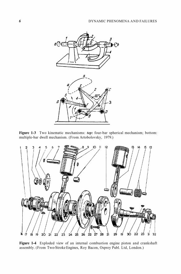
The subject of multilink kinematics is an old field with a long history. The collection of linkage systems by F. Reuleaux in Germany for teaching kinematics in the nineteenth Century has yet to be rivaled in this century. And the beautiful catalog of kinematic mechanisms by the Russian Arto- bolsky (see the References section) shows the great variety of devices for creating motion in a mechanical system (Figure 1-3). See Erdman (1993) for a review of modern kinematics.

One of the world’s most ubiquitous simple multibody mechanisms is the slider crank (Figure 1-4) used in internal combustion engines. Earlier dynamic analysis of the forces in such systems used graphical methods. Today there are powerful commercial and research codes to analyze and graphically simulate the motions of complicated dynamic systems (see Schiehlen, 1990).

One of the recent tools has been the use of graph theory to represent the connectedness topology of the multibody system. Figure 1-5 shows chain, closed-loop, and tree-type multibody geometries. The classic serial link


C

3

Figure 1-3 Two kinematic mechanisms: top: four-bar spherical mechanism; bottom: multiple-bar dwell mechanism. (From Artobolovsky, 1979.)

Figure 1-4 Exploded view of an internal combustion engine piston and crankshaft assembly. (From Two-Stroke Engines, Roy Bacon, Osprey Publ. Ltd, London.)

1.2 WHAT'S NEW IN DYNAMICS? 7

Chain

Closed Loop

Tree Structure

Figure 1-5 Linked multibody systems: top: chain structure; middle: closed-loop structure; bottom: tree structure.

mechanism (Figure 1-6) can be an open chain, a closed chain or a loop structure if it comes in contact with its base environment. Some of the most difficult dynamics problems in these systems are friction, impact, and rolling contracts, which still require more research. Practical examples of multibody


p Pitch

Figure 1-6 Serial-link robotic manipulator arm showing kinematic degrees of freedom. (From Rosheim, 1995. Reprinted with permission.)

1.2 WHAT'S NEW IN DYNAMICS? 9

systems include:

0 Robotic devices 0 Door and latch mechanisms in aircraft design, jigs, and fixtures 0 Train, tandum trucks, and buses 0 Docking of space vehicles 0 Solar panel deployment on satellites 0 Helicopters 0 Biomechanical systems: walking and mobility prosthetics

Modern texts in multibody dynamics include Huston (1990), Shabana (1989), Roberson and Schwertassek (1988) and Wittenburg (1977).

Mechatvonics Other names are used for this class of problems, including controlled machines, smart machines and structures, and intelligent machines. However the term, mechatronics is in use in Europe and Japan where mechatronic devices such as magnetic bearings and automated cameras and video equipment have been pioneered. One of the large-scale applications of mechatronics is the Mag-Lev train shown in Figure 1-7 that has been developed in Japan and Germany. Active magnetic bearings for large and small rotary machines such as gas pipeline pumps and machine tool spindles have been pioneered in Switzerland, France, and Japan. (see e.g., Moon, 1994). In the United States a significant amount of research and development has been directed toward microelectromechanical systems or MEMS (Figure 1-8).

The distinguishing feature of most of these systems compared to tradi- tional controlled machines, has been the incorporation of sensing, actuation, and intelligence in producing and controlling motion in machines and structures. Thus the engineer is called on to integrate control and intelligence into the mechanical design from the very beginning and not as an add-on after the machine is designed. For example, the control motions at the joints of serial robot arms will effect the dynamics of manipulation and must be optimized along with the rest of the system.

New Methods of Computation

The development of microprocessors, workstations, and computer graphics has resulted in a plethora of codes and software to solve particle, rigid body, and coupled elastic body dynamics problems (see Appendix B and Schiehlen, 1990). An example is shown in Figure 1-9. Often, however, the methods of formulation and solution of dynamic problems are not transparent to the user who cannot assess the limitation of such codes.

These new codes allow one to specify geometry, materials, and the type of joints and constraints. The derivation of equations of motion is hidden from


Superconducting magnet

(bl

Figure 1-7 Sketch of two Mag-Lev systems (a) Electromagnetic levitation (EML), which requires electronic feedback control. (b) Electrodynamic levitation using superconducting magnets. (From Moon, 1994)

the user. The integrated motions are presented in the form of computer- generated graphs and movie frame simulation of the moving objects. Two of the major workstation codes in use are DADS and ADAMS and another for the PC is Working Model.

An intermediate level code for dynamic analysis is MATLAB. Here the user must provide the equations of motion and MATLAB will numerically integrate and display the results graphically. A few examples of the use of MATLAB are given in this text.

In addition to these numerical codes, however, software to perform symbolic mathematical operations have appeared, such as MACSYMA, MAPLE, and MATHEMATICA. A few examples of the use of these codes to derive equations of motion are given in this text.

1.2 WHAT’S NEW IN DYNAMICS? 11

Figure 1-8 substrate. See also Chapter 8, Figure 8-24. (Courtesy Adams, 1996.)

Microelectromechanical (MEMS) accelerometer photoetched from a silicon

New Experimental Tools

In the last two decades the ability of the dynamicist and the engineer to observe and measure dynamical systems has been greatly enhanced by new sensors, signal processing, and actuator devices for control.


. ..;. .............

.......... .:. ....

...; .............

..-: ......; ......

... ; ....... \ ..... ' W

.. .> ...... ;. ....

.. ; ..............

........... ; ..... Figure 1-9 Still cartoon frame from a dynamic simulation code using Working Model software. (See also Appendix B)

Sensing and Measurement Systems The two most important developments have been optical sensing systems and video recording. These include:

0 Optical follower cameras for large motions 0 Fiber-optic proximity systems for small motions 0 Optical encoders for rotary and linear motions 0 Holographic methods for elastic deformation 0 High-speed framing cameras 0 X-Ray methods 0 Portable video scanning cameras

1.3 DYNAMIC FAILURES 13

Signal Processing Methods There are four basic signal-processing systems for storing data from dynamical systems; analog and digital oscilloscopes, dedicated signal analysis electronics, and computer hardware, such as hard drives. These devices are either directly connected to sensing electronics or a buffer is used, such as a data-acquisition system. Many measurement systems use a direct input to a computer or microprocessor where the data are analyzed in software.

One of the important advances in dynamic measurement has been the invention of the fast Fourier transform chip (FFT). This allows on-line calculation of dynamic Fourier transforms or spectra, which in the past required post-data-acquisition processing.

System Zdentijication: Linear Systems This field has seen the development of software tools to allow the construction of a linear mathematical model (usually differential or difference equations) from a digitally sampled dynamic data record. In some systems where the data are sampled at different spatial locations on the machine or structure, the spatial eigenmodes can also be reconstructed. In control systems that use model-based feedback, algo- rithms such as Kalman filters are used to obtain an approximate model of the system under control.

System Identification: Nonlinear Systems Methods for nonlinear dynamical systems are under continual development. In recent years the development of Chaos Theory (Chapter 9) has produced an evolving methodology based on constructing the topological and geometric features of the dynamical object in phase space. New techniques based on time series sampling of dynamic records such as fractal dimension and false nearest neighbors, allow us to place a bound on the dimension of the phase space (see Moon, 1992; Abarbanel, 1996).

Other methods, such as Poincare maps (Chapter 9) and bifurcation diagrams, have been used to characterize the nature of motions in nonlinear systems.

1.3 DYNAMIC FAILURES

While dynamic analysis in engineering is often used to create motions in physical systems, in many cases unwanted dynamic failures are to be avoided. Such failures include:

0 Large deflections 0 Fatigue 0 Motion-induced fracture 0 Dynamic instability, e.g., flutter, chatter, wheel shimmy 0 Impact-induced local damage


0 Dynamic buckling in structures 0 Motion-included noise 0 Instability about a steady motion, e.g., wheel on rails 0 Thermal heating due to dynamic friction

A few of the most important failure modes are fatigue, dynamic instability, and noise.

Fatigue

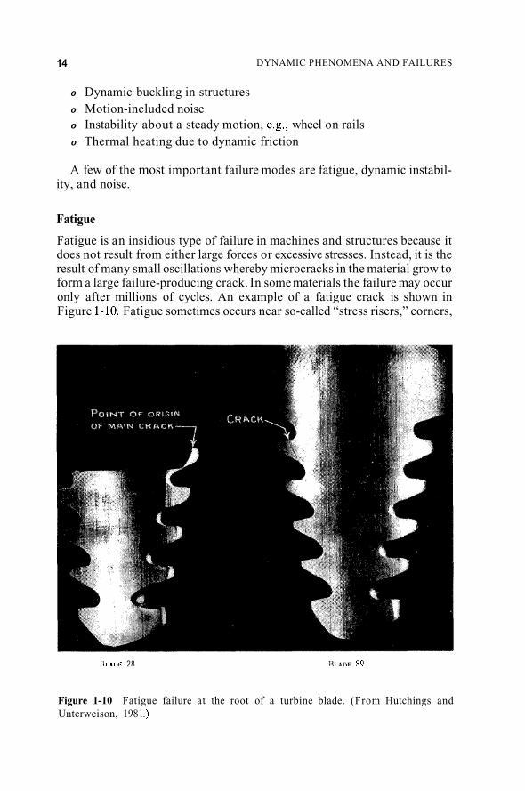
Fatigue is an insidious type of failure in machines and structures because it does not result from either large forces or excessive stresses. Instead, it is the result of many small oscillations whereby microcracks in the material grow to form a large failure-producing crack. In some materials the failure may occur only after millions of cycles. An example of a fatigue crack is shown in Figure 1-10, Fatigue sometimes occurs near so-called “stress risers,” corners,

BLADE 28 RI..4DE 89

Figure 1-10 Unterweison, 198 1 .)

Fatigue failure at the root of a turbine blade. (From Hutchings and

1.3 DYNAMIC FAILURES 15

Number of cycles

0.001 I I I I I I I

0.1 1 10 lo2 103 1 o4 1 o5 Number of cycles

1.0 r

0.001 I I I I 1 I

0.1 1 10 lo2 103 1 o4 Number of cycles

Figure 1-11 S-N Curve: Plastic strain vs. cycles to failure. Top: aluminum, commerically pure; middle: titanium, commercially pure; bottom: Zn-A1 alloy. (From Frost et al., 1974.)


holes, etc. But fatigue can also occur through repeated dynamic contact such as in gear teeth in transmissions or rolling problems in rail-wheel systems. A standard plot of dynamic stress vs. number of cycles to failure is shown in Figure 1-1 1 for aluminum and titanium. In the case of steel there sometimes exists a dynamic stress below which cracks don’t grown, a so-called “fatigue limit stress.” In the case of aluminum, however, a limit doesn’t exist, so any level of repeated stress will eventually lead to failure. Fatigue is one reason why the study of small vibrations is such an important subgroup of dynamics. (See e.g., Frost et al., 1974.)

Dynamic Instabilities

Many machines are designed to operate in a steady dynamic state character- ized by a constant velocity, such as an aircraft or constant rotation as in turbines and generators. A satellite pointing toward the earth involves both steady translation and rotation. One classic failure mode in these machines is a significant departure from steady state. Examples include:

0 Wing flutter Machine tool chatter Vehicle skidding, wheel shimmy

e Train derailment 0 Uncontrollable spin of aircraft

In many of these systems, a linear stability analysis can be performed. As an example consider the lateral-yaw motions of a Mag-Lev vehicle moving along a guideway, shown in Figure 1-12 (see Chapter 8, also Moon, 1994). The lateral motion of the center of mass, u, and the yaw, 4, can be modelled as two coupled oscillators:

where some of the constants depend on the steady velocity parameter, Vo. In linear stability analysis, one looks for a solution of the form

[ ;] = [ This problem results in a so-called eigenvalueproblem. In general there might be two such solutions, i.e., two sets of { A i , Bi, si} where s1 = f ( V o ) , s2 = g( Vo). These values can be complex, i.e., si = ai + iPi.

When ai = 0, we say the mode is oscillatory; ai < 0, Pi # 0, the system is

APPLIED DYNAMICS - download.e-bookshelf.de · APPLIED DYNAMICS With Applications to Multibody and...

Documents

Transcript of APPLIED DYNAMICS - download.e-bookshelf.de · APPLIED DYNAMICS With Applications to Multibody and...