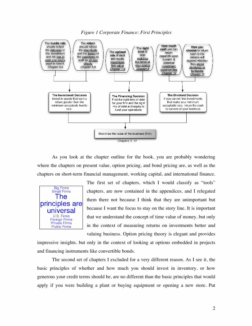
1

Preface Let me begin this preface with a confession of a few of my own biases. First, I

believe that theory and the models that flow from it should provide the tools to

understand, analyze, and solve problems. The test of a model or theory then should not be

based on its elegance but on its usefulness in problem solving. Second, there is little in

corporate financial theory that is new and revolutionary. The core principles of corporate

finance are common sense and have changed little over time. That should not be

surprising. Corporate finance is only a few decades old, and people have been running

businesses for thousands of years; it would be exceedingly presumptuous of us to believe

that they were in the dark until corporate finance theorists came along and told them what

to do. To be fair, it is true that corporate financial theory has made advances in taking

commonsense principles and providing structure, but these advances have been primarily

on the details. The story line in corporate finance has remained remarkably consistent

over time.

Talking about story lines allows me to set the first theme of this book. This book

tells a story, which essentially summarizes the corporate finance view of the world. It

classifies all decisions made by any business into three groups—decisions on where to

invest the resources or funds that the business has raised, either internally or externally

(the investment decision), decisions on where and how to raise funds to finance these

investments (the financing decision), and decisions on how much and in what form to

return funds back to the owners (the dividend decision). As I see it, the first principles of

corporate finance can be summarized in Figure 1, which also lays out a site map for the

book. Every section of this book relates to some part of this picture, and each chapter is

introduced with it, with emphasis on that portion that will be analyzed in that chapter.

(Note the chapter numbers below each section). Put another way, there are no sections of

this book that are not traceable to this framework.

2

Figure 1 Corporate Finance: First Principles

As you look at the chapter outline for the book, you are probably wondering

where the chapters on present value, option pricing, and bond pricing are, as well as the

chapters on short-term financial management, working capital, and international finance.

The first set of chapters, which I would classify as “tools”

chapters, are now contained in the appendices, and I relegated

them there not because I think that they are unimportant but

because I want the focus to stay on the story line. It is important

that we understand the concept of time value of money, but only

in the context of measuring returns on investments better and

valuing business. Option pricing theory is elegant and provides

impressive insights, but only in the context of looking at options embedded in projects

and financing instruments like convertible bonds.

The second set of chapters I excluded for a very different reason. As I see it, the

basic principles of whether and how much you should invest in inventory, or how

generous your credit terms should be, are no different than the basic principles that would

apply if you were building a plant or buying equipment or opening a new store. Put

3

another way, there is no logical basis for the differentiation between investments in the

latter (which in most corporate finance books is covered in the capital budgeting

chapters) and the former (which are considered in the working capital chapters). You

should invest in either if and only if the returns from the investment exceed the hurdle

rate from the investment; the fact the one is short-term and the other is long-term is

irrelevant. The same thing can be said about international finance. Should the investment

or financing principles be different just because a company is considering an investment

in Thailand and the cash flows are in Thai baht instead of in the United States, where the

cash flows are in dollars? I do not believe so, and in my view separating the decisions

only leaves readers with that impression. Finally, most corporate finance books that have

chapters on small firm management and private firm management use them to illustrate

the differences between these firms and the more conventional large publicly traded firms

used in the other chapters. Although such differences exist, the commonalities between

different types of firms vastly overwhelm the differences, providing a testimonial to the

internal consistency of corporate finance. In summary, the second theme of this book is

the emphasis on the universality of corporate financial principles across different firms,

in different markets, and across different types of

decisions.

The way I have tried to bring this universality

to life is by using five firms through the book to

illustrate each concept; they include a large, publicly

traded U.S. corporation (Disney); a small, emerging market commodity company

(Aracruz Celulose, a Brazilian paper and pulp company); an Indian manufacturing

company that is part of a family group (Tata Chemicals), a financial service firm

(Deutsche Bank); and a small private business (Bookscape, an independent New York

City bookstore). Although the notion of using real companies to illustrate theory is

neither novel nor revolutionary, there are, two key differences in the way they are used in

this book. First, these companies are analyzed on every aspect of corporate finance

introduced here, rather than just selectively in some chapters. Consequently, the reader

can see for him- or herself the similarities and the differences in the way investment,

financing, and dividend principles are applied to four very different firms. Second, I do

4

not consider this to be a book where applications are used to illustrate theory but a book

where the theory is presented as a companion to the illustrations. In fact, reverting back

to my earlier analogy of theory providing the tools for understanding problems, this is a

book where the problem solving takes center stage and the tools stay in the background.

Reading through the theory and the applications can be instructive and even

interesting, but there is no substitute for actually trying things out to bring home both the

strengths and weaknesses of corporate finance. There are several ways I have made this

book a tool for active learning. One is to introduce concept questions at regular intervals

that invite responses from the reader. As an example, consider the following illustration

from Chapter 7:

7.2. The Effects of Diversification on Venture Capitalist

You are comparing the required returns of two venture capitalists who are interested in

investing in the same software firm. One has all of his capital invested in only software

firms, whereas the other has invested her capital in small companies in a variety of

businesses. Which of these two will have the higher required rate of return?

❒ The venture capitalist who is invested only in software companies.

❒ The venture capitalist who is invested in a variety of businesses.

❒ Cannot answer without more information.

This question is designed to check on a concept introduced in an earlier chapter

on risk and return on the difference between risk that can be eliminated by holding a

diversified portfolio and risk that cannot and then connecting it to the question of how a

business seeking funds from a venture capitalist might be affected by this perception of

risk. The answer to this question in turn will expose the reader to more questions about

whether venture capital in the future will be provided by diversified funds and what a

specialized venture capitalist (who invests in one

sector alone) might need to do to survive in such an

environment. This will allow readers to see what, for

me at least, is one of the most exciting aspects of

corporate finance—its capacity to provide a

5

framework that can be used to make sense of the events that occur around us every day

and make reasonable forecasts about future directions.

The second active experience in this book is found in the Live Case Studies at the

end of each chapter. These case studies essentially take the concepts introduced in the

chapter and provide a framework for applying them to any company the reader chooses.

Guidelines on where to get the information to answer the questions are also provided.

Although corporate finance provides an internally consistent and straightforward

template for the analysis of any firm, information is

clearly the lubricant that allows us to do the analysis.

There are three steps in the information process—

acquiring the information, filtering what is useful

from what is not, and keeping the information

updated. Accepting the limitations of the printed page on all of these aspects, I have put

the power of online information to use in several ways.

1. The case studies that require the information are accompanied by links to Web sites

that carry this information.

2. The data sets that are difficult to get from the Internet or are specific to this book,

such as the updated versions of the tables, are available on my own Web site

(www.damodaran.com) and are integrated into the book. As an example, the table

that contains the dividend yields and payout ratios by industry sectors for the most

recent quarter is referenced in Chapter 9 as follows:

There is a data set online that summarizes dividend yields and payout ratios for

U.S. companies, categorized by sector.

You can get to this table by going to the website for the book and checking for

datasets under chapter 9.

3. The spreadsheets used to analyze the firms in the book are also available on my Web

site and are referenced in the book. For instance, the spreadsheet used to estimate the

optimal debt ratio for Disney in Chapter 8 is referenced as follows:

6

Capstru.xls : This spreadsheet allows you to compute the optimal debt ratio firm

value for any firm, using the same information used for Disney. It has updated

interest coverage ratios and spreads built in.

As with the dataset listing above, you can get this spreadsheet by going to the

website for the book and checking under spreadsheets under chapter 8.

For those of you have read the first two editions of this book, much of what I have

said in this preface should be familiar. But there are three places where you will find this

book to be different:

a. For better or worse, the banking and market crisis of 2008 has left lasting wounds

on our psyches as investors and shaken some of our core beliefs in how to

estimate key numbers and approach fundamental trade offs. I have tried to adapt

some of what I have learned about equity risk premiums and the distress costs of

debt into the discussion.

b. I have always been skeptical about behavioral finance but I think that the area has

some very interesting insights on how managers behave that we ignore at our own

peril. I have made my first foray into incorporating some of the work in

behavioral financing into investing, financing and dividend decisions.

As I set out to write this book, I had two objectives in mind. One was to write a book that

not only reflects the way I teach corporate finance in a classroom but, more important,

conveys the fascination and enjoyment I get out of the subject matter. The second was to

write a book for practitioners that students would find useful, rather than the other way

around. I do not know whether I have fully accomplished either objective, but I do know

I had an immense amount of fun trying. I hope you do, too!

1.1

1

CHAPTER 1

THE FOUNDATIONS

It’s all corporate finance.

My unbiased view of the world

Every decision made in a business has financial implications, and any decision

that involves the use of money is a corporate financial decision. Defined broadly,

everything that a business does fits under the rubric of corporate finance. It is, in fact,

unfortunate that we even call the subject corporate finance, because it suggests to many

observers a focus on how large corporations make financial decisions and seems to

exclude small and private businesses from its purview. A more appropriate title for this

book would be Business Finance, because the basic principles remain the same, whether

one looks at large, publicly traded firms or small, privately run businesses. All businesses

have to invest their resources wisely, find the right kind and mix of financing to fund

these investments, and return cash to the owners if there are not enough good

investments.

In this chapter, we will lay the foundation for the rest of the book by listing the

three fundamental principles that underlie corporate finance—the investment, financing,

and dividend principles—and the objective of firm value maximization that is at the heart

of corporate financial theory.

The Firm: Structural Set-Up In the chapters that follow, we will use firm generically to refer to any business,

large or small, manufacturing or service, private or public. Thus, a corner grocery store

and Microsoft are both firms.

The firm’s investments are generically termed assets. Although assets are often

categorized by accountants into fixed assets, which are long-lived, and current assets,

which are short-term, we prefer a different categorization. The assets that the firm has

already invested in are called assets in place, whereas those assets that the firm is

1.2

2

expected to invest in the future are called growth assets. Though it may seem strange

that a firm can get value from investments it has not made yet, high-growth firms get the

bulk of their value from these yet-to-be-made investments.

To finance these assets, the firm can raise money from two sources. It can raise

funds from investors or financial institutions by promising investors a fixed claim

(interest payments) on the cash flows generated by the assets, with a limited or no role in

the day-to-day running of the business. We categorize this type of financing to be debt. Alternatively, it can offer a residual claim on the cash flows (i.e., investors can get what

is left over after the interest payments have been made) and a much greater role in the

operation of the business. We call this equity. Note that these definitions are general

enough to cover both private firms, where debt may take the form of bank loans and

equity is the owner’s own money, as well as publicly traded companies, where the firm

may issue bonds (to raise debt) and common stock (to raise equity).

Thus, at this stage, we can lay out the financial balance sheet of a firm as follows:

We will return this framework repeatedly through this book.

First Principles Every discipline has first principles that govern and guide everything that gets

done within it. All of corporate finance is built on three principles, which we will call,

rather unimaginatively, the investment principle, the financing principle, and the dividend

principle. The investment principle determines where businesses invest their resources,

the financing principle governs the mix of funding used to fund these investments, and

the dividend principle answers the question of how much earnings should be reinvested

back into the business and how much returned to the owners of the business. These core

corporate finance principles can be stated as follows:

1.3

3

• The Investment Principle: Invest in assets and projects that yield a return greater

than the minimum acceptable hurdle rate. The hurdle rate should be higher for riskier

projects and should reflect the financing mix used—owners’ funds (equity) or

borrowed money (debt). Returns on projects should be measured based on cash flows

generated and the timing of these cash flows; they should also consider both positive

and negative side effects of these projects.

• The Financing Principle: Choose a financing mix (debt and equity) that maximizes

the value of the investments made and match the financing to the nature of the assets

being financed.

• The Dividend Principle: If there are not enough investments that earn the hurdle rate,

return the cash to the owners of the business. In the case of a publicly traded firm, the

form of the return—dividends or stock buybacks—will depend on what stockholders

prefer.

When making investment, financing and dividend decisions, corporate finance is

single-minded about the ultimate objective, which is assumed to be maximizing the value

of the business. These first principles provide the basis from which we will extract the

numerous models and theories that comprise modern corporate finance, but they are also

commonsense principles. It is incredible conceit on our part to assume that until corporate

finance was developed as a coherent discipline starting just a few decades ago, people

who ran businesses made decisions randomly with no principles to govern their thinking.

Good businesspeople through the ages have always recognized the importance of these

first principles and adhered to them, albeit in intuitive ways. In fact, one of the ironies of

recent times is that many managers at large and presumably sophisticated firms with

access to the latest corporate finance technology have lost sight of these basic principles.

The Objective of the Firm

No discipline can develop cohesively over time without a unifying objective. The

growth of corporate financial theory can be traced to its choice of a single objective and

the development of models built around this objective. The objective in conventional

corporate financial theory when making decisions is to maximize the value of the

business or firm. Consequently, any decision (investment, financial, or dividend) that

1.4

4

increases the value of a business is considered a good one, whereas one that reduces firm

value is considered a poor one. Although the choice of a singular objective has provided

corporate finance with a unifying theme and internal consistency, it comes at a cost. To

the degree that one buys into this objective, much of what corporate financial theory

posits makes sense. To the degree that this objective is flawed, however, it can be argued

that the theory built on it is flawed as well. Many of the disagreements between corporate

financial theorists and others (academics as well as practitioners) can be traced to

fundamentally different views about the correct objective for a business. For instance,

there are some critics of corporate finance who argue that firms should have multiple

objectives where a variety of interests (stockholders, labor, customers) are met, and there

are others who would have firms focus on what they view as simpler and more direct

objectives, such as market share or profitability.

Given the significance of this objective for both the development and the

applicability of corporate financial theory, it is important that we examine it much more

carefully and address some of the very real concerns and criticisms it has garnered: It

assumes that what stockholders do in their own self-interest is also in the best interests of

the firm, it is sometimes dependent on the existence of efficient markets, and it is often

blind to the social costs associated with value maximization. In the next chapter, we

consider these and other issues and compare firm value maximization to alternative

objectives.

The Investment Principle

Firms have scarce resources that must be

allocated among competing needs. The first and

foremost function of corporate financial theory is to

provide a framework for firms to make this decision

wisely. Accordingly, we define investment decisions to include not only those that create

revenues and profits (such as introducing a new product line or expanding into a new

market) but also those that save money (such as building a new and more efficient

distribution system). Furthermore, we argue that decisions about how much and what

inventory to maintain and whether and how much credit to grant to customers that are

Hurdle Rate: A hurdle rate is a

minimum acceptable rate of return for

investing resources in a new investment.

1.5

5

traditionally categorized as working capital decisions, are ultimately investment decisions

as well. At the other end of the spectrum, broad strategic decisions regarding which

markets to enter and the acquisitions of other companies can also be considered

investment decisions.

Corporate finance attempts to measure the return on a proposed investment

decision and compare it to a minimum acceptable hurdle rate to decide whether the

project is acceptable. The hurdle rate has to be set higher for riskier projects and has to

reflect the financing mix used, i.e., the owner’s funds (equity) or borrowed money (debt).

In Chapter 3, we begin this process by defining risk and developing a procedure for

measuring risk. In Chapter 4, we go about converting this risk measure into a hurdle rate,

i.e., a minimum acceptable rate of return, both for entire businesses and for individual

investments.

Having established the hurdle rate, we turn our attention to measuring the returns

on an investment. In Chapter 5 we evaluate three alternative ways of measuring returns—

conventional accounting earnings, cash flows, and time-weighted cash flows (where we

consider both how large the cash flows are and when they are anticipated to come in). In

Chapter 6 we consider some of the potential side costs that might not be captured in any

of these measures, including costs that may be created for existing investments by taking

a new investment, and side benefits, such as options to enter new markets and to expand

product lines that may be embedded in new investments, and synergies, especially when

the new investment is the acquisition of another firm.

The Financing Principle

Every business, no matter how large and complex, is ultimately funded with a mix

of borrowed money (debt) and owner’s funds (equity). With a publicly trade firm, debt

may take the form of bonds and equity is usually common stock. In a private business,

debt is more likely to be bank loans and an owner’s savings represent equity. Though we

consider the existing mix of debt and equity and its implications for the minimum

acceptable hurdle rate as part of the investment principle, we throw open the question of

whether the existing mix is the right one in the financing principle section. There might

be regulatory and other real-world constraints on the financing mix that a business can

1.6

6

use, but there is ample room for flexibility within these constraints. We begin this section

in Chapter 7, by looking at the range of choices that exist for both private businesses and

publicly traded firms between debt and equity. We then turn to the question of whether

the existing mix of financing used by a business is optimal, given the objective function

of maximizing firm value, in Chapter 8. Although the trade-off between the benefits and

costs of borrowing are established in qualitative terms first, we also look at quantitative

approaches to arriving at the optimal mix in Chapter 8. In the first approach, we examine

the specific conditions under which the optimal financing mix is the one that minimizes

the minimum acceptable hurdle rate. In the second approach, we look at the effects on

firm value of changing the financing mix.

When the optimal financing mix is different from the existing one, we map out

the best ways of getting from where we are (the current mix) to where we would like to

be (the optimal) in Chapter 9, keeping in mind the investment opportunities that the firm

has and the need for timely responses, either because the firm is a takeover target or

under threat of bankruptcy. Having outlined the optimal financing mix, we turn our

attention to the type of financing a business should use, such as whether it should be

long-term or short-term, whether the payments on the financing should be fixed or

variable, and if variable, what it should be a function of. Using a basic proposition that a

firm will minimize its risk from financing and maximize its capacity to use borrowed

funds if it can match up the cash flows on the debt to the cash flows on the assets being

financed, we design the perfect financing instrument for a firm. We then add additional

considerations relating to taxes and external monitors (equity research analysts and

ratings agencies) and arrive at strong conclusions about the design of the financing.

The Dividend Principle

Most businesses would undoubtedly like to have unlimited investment

opportunities that yield returns exceeding their hurdle rates, but all businesses grow and

mature. As a consequence, every business that thrives reaches a stage in its life when the

cash flows generated by existing investments is greater than the funds needed to take on

good investments. At that point, this business has to figure out ways to return the excess

cash to owners In private businesses, this may just involve the owner withdrawing a

1.7

7

portion of his or her funds from the business. In a publicly traded corporation, this will

involve either paying dividends or buying back stock. Note that firms that choose not to

return cash to owners will accumulate cash balances that grow over time. Thus, analyzing

whether and how much cash should be returned to the owners of a firm is the equivalent

of asking (and answering) the question of how much cash accumulated in a firm is too

much cash.

In Chapter 10, we introduce the basic trade-off that determines whether cash

should be left in a business or taken out of it. For stockholders in publicly traded firms,

we note that this decision is fundamentally one of whether they trust the managers of the

firms with their cash, and much of this trust is based on how well these managers have

invested funds in the past. In Chapter 11, we consider the options available to a firm to

return assets to its owners—dividends, stock buybacks and spin-offs—and investigate

how to pick between these options.

Corporate Financial Decisions, Firm Value, and Equity Value If the objective function in corporate finance is to maximize firm value, it follows

that firm value must be linked to the three corporate finance decisions outlined—

investment, financing, and dividend decisions. The link between these decisions and firm

value can be made by recognizing that the value of a firm is the present value of its

expected cash flows, discounted back at a rate that reflects both the riskiness of the

projects of the firm and the financing mix used to finance them. Investors form

expectations about future cash flows based on observed current cash flows and expected

future growth, which in turn depend on the quality of the firm’s projects (its investment

decisions) and the amount reinvested back into the business (its dividend decisions). The

financing decisions affect the value of a firm through both the discount rate and

potentially through the expected cash flows.

This neat formulation of value is put to the test by the interactions among the

investment, financing, and dividend decisions and the conflicts of interest that arise

between stockholders and lenders to the firm, on one hand, and stockholders and

managers, on the other. We introduce the basic models available to value a firm and its

equity in Chapter 12, and relate them back to management decisions on investment,

1.8

8

financial, and dividend policy. In the process, we examine the determinants of value and

how firms can increase their value.

A Real-World Focus The proliferation of news and information on real-world businesses making

decisions every day suggests that we do not need to use hypothetical examples to

illustrate the principles of corporate finance. We will use five businesses through this

book to make our points about corporate financial policy:

1. Disney Corporation: Disney Corporation is a publicly traded firm with wide holdings

in entertainment and media. Most people around the world recognize the Mickey

Mouse logo and have heard about or visited a Disney theme park or seen some or all

of the Disney animated classic movies, but it is a much more diversified corporation

than most people realize. Disney’s holdings include cruise line, real estate (in the

form of time shares and rental properties in Florida and South Carolina), television

(Disney cable, ABC and ESPN), publications, movie studios (Miramax, Pixar and

Disney) and consumer products. Disney will help illustrate the decisions that large

multi-business and multinational corporations have to make as they are faced with the

conventional corporate financial decisions—Where do we invest? How do we finance

these investments? How much do we return to our stockholders?

2. Bookscape Books: This company is a privately owned independent bookstore in New

York City, one of the few left after the invasion of the bookstore chains, such as

Barnes and Noble and Borders. We will take Bookscape Books through the corporate

financial decision-making process to illustrate some of the issues that come up when

looking at small businesses with private owners.

3. Aracruz Celulose: Aracruz Celulose is a Brazilian firm that produces eucalyptus pulp

and operates its own pulp mills, electrochemical plants, and port terminals. Although

it markets its products around the world for manufacturing high-grade paper, we use

it to illustrate some of the questions that have to be dealt with when analyzing a

company that is highly dependent upon commodity prices – paper and pulp, in this

instance, and operates in an environment where inflation is high and volatile and the

economy itself is in transition.

1.9

9

4. Deutsche Bank: Deutsche Bank is the leading commercial bank in Germany and is

also a leading player in investment banking. We will use Deutsche Bank to illustrate

some of the issues the come up when a financial service firm has to make investment,

financing and dividend decisions. Since banks are highly regulated institutions, it will

also serve to illustrate the constraints and opportunities created by the regulatory

framework.

5. Tata Chemicals: Tata Chemicals is a firm involved in the chemical and fertilizer

business and is part of one of the largest Indian family group companies, the Tata

Group, with holdings in technology, manufacturing and service businesses. In

addition to allowing us to look at issues specific to manufacturing firms, Tata

Chemicals will also give us an opportunity to examine how firms that are part of

larger groups make corporate finance decisions.

We will look at every aspect of finance through the eyes of all five companies, sometimes

to draw contrasts between the companies, but more often to show how much they share.

A Resource Guide To make the learning in this book as interactive and current as possible, we

employ a variety of devices.

This icon indicates that spreadsheet programs can be used to do some of the

analysis that will be presented. For instance, there are spreadsheets that calculate the

optimal financing mix for a firm as well as valuation spreadsheets.

This symbol marks the second supporting device: updated data on some of the

inputs that we need and use in our analysis that is available online for this book. Thus,

when we estimate the risk parameters for firms, we will draw attention to the data set

that is maintained online that reports average risk parameters by industry.

At regular intervals, we will also ask readers to answer questions relating to a

topic. These questions, which will generally be framed using real-world examples,

will help emphasize the key points made in a chapter and will be marked with this

icon.

1.10

10

✄ .In each chapter, we will introduce a series of boxes titled “In Practice,” which will

look at issues that are likely to come up in practice and ways of addressing these

issues.

We examine how firms behave when it comes to assessing risk, evaluating

investments and determining the mix off debt and equity, and dividend policy. To

make this assessment, we will look at both surveys of decision makers (which

chronicle behavior at firms) as well as the findings from studies in behavioral finance

that try to explain patterns of management behavior.

Some Fundamental Propositions about Corporate Finance There are several fundamental arguments we will make repeatedly throughout this

book.

1. Corporate finance has an internal consistency that flows from its choice of

maximizing firm value as the only objective function and its dependence on a few

bedrock principles: Risk has to be rewarded, cash flows matter more than accounting

income, markets are not easily fooled, and every decision a firm makes has an effect on

its value.

2. Corporate finance must be viewed as an integrated whole, rather than a collection of

decisions. Investment decisions generally affect financing decisions and vice versa;

financing decisions often influence dividend decisions and vice versa. Although there are

circumstances under which these decisions may be independent of each other, this is

seldom the case in practice. Accordingly, it is unlikely that firms that deal with their

problems on a piecemeal basis will ever resolve these problems. For instance, a firm that

takes poor investments may soon find itself with a dividend problem (with insufficient

funds to pay dividends) and a financing problem (because the drop in earnings may

make it difficult for them to meet interest expenses).

3. Corporate finance matters to everybody. There is a corporate financial aspect to almost

every decision made by a business; though not everyone will find a use for all the

components of corporate finance, everyone will find a use for at least some part of it.

Marketing managers, corporate strategists, human resource managers, and information

1.11

11

technology managers all make corporate finance decisions every day and often don’t

realize it. An understanding of corporate finance will help them make better decisions.

4. Corporate finance is fun. This may seem to be the tallest claim of all. After all, most

people associate corporate finance with numbers, accounting statements, and hardheaded

analyses. Although corporate finance is quantitative in its focus, there is a significant

component of creative thinking involved in coming up with solutions to the financial

problems businesses do encounter. It is no coincidence that financial markets remain

breeding grounds for innovation and change.

5. The best way to learn corporate finance is by applying its models and theories to real-

world problems. Although the theory that has been developed over the past few decades

is impressive, the ultimate test of any theory is application. As we show in this book,

much (if not all) of the theory can be applied to real companies and not just to abstract

examples, though we have to compromise and make assumptions in the process.

Conclusion This chapter establishes the first principles that govern corporate finance. The

investment principle specifies that businesses invest only in projects that yield a return

that exceeds the hurdle rate. The financing principle suggests that the right financing mix

for a firm is one that maximizes the value of the investments made. The dividend

principle requires that cash generated in excess of good project needs be returned to the

owners. These principles are the core for what follows in this book.

2.1

1

CHAPTER 2

THE OBJECTIVE IN DECISION MAKING

If you do not know where you are going, it does not matter how you get there.

Anonymous

Corporate finance’s greatest strength and greatest weakness is its focus on value

maximization. By maintaining that focus, corporate finance preserves internal

consistency and coherence and develops powerful models and theory about the right way

to make investment, financing, and dividend decisions. It can be argued, however, that all

of these conclusions are conditional on the acceptance of value maximization as the only

objective in decision-making.

In this chapter, we consider why we focus so strongly on value maximization and

why, in practice, the focus shifts to stock price maximization. We also look at the

assumptions needed for stock price maximization to be the right objective, what can go

wrong with firms that focus on it, and at least partial fixes to some of these problems. We

will argue strongly that even though stock price maximization is a flawed objective, it

offers far more promise than alternative objectives because it is self-correcting.

Choosing the Right Objective Let’s start with a description of what an objective is and the purpose it serves in

developing theory. An objective specifies what a decision maker is trying to accomplish

and by so doing provides measures that can be used to choose between alternatives. In

most firms, the managers of the firm, rather than the owners, make the decisions about

where to invest or how to raise funds for an investment. Thus, if stock price

maximization is the objective, a manager choosing between two alternatives will choose

the one that increases stock price more. In most cases, the objective is stated in terms of

maximizing some function or variable, such as profits or growth, or minimizing some

function or variable, such as risk or costs.

So why do we need an objective, and if we do need one, why can’t we have

several? Let’s start with the first question. If an objective is not chosen, there is no

2.2

2

systematic way to make the decisions that every business will be confronted with at some

point in time. For instance, without an objective, how can Disney’s managers decide

whether the investment in a new theme park is a good one? There would be a menu of

approaches for picking projects, ranging from reasonable ones like maximizing return on

investment to obscure ones like maximizing the size of the firm, and no statements could

be made about their relative value. Consequently, three managers looking at the same

project may come to three separate conclusions.

If we choose multiple objectives, we are faced with a different problem. A theory

developed around multiple objectives of equal weight will create quandaries when it

comes to making decisions. For example, assume that a firm chooses as its objectives

maximizing market share and maximizing current earnings. If a project increases market

share and current earnings, the firm will face no problems, but what if the project under

analysis increases market share while reducing current earnings? The firm should not

invest in the project if the current earnings objective is considered, but it should invest in

it based on the market share objective. If objectives are prioritized, we are faced with the

same stark choices as in the choice of a single objective. Should the top priority be the

maximization of current earnings or should it be maximizing market share? Because there

is no gain, therefore, from having multiple objectives, and developing theory becomes

much more difficult, we argue that there should be only one objective.

There are a number of different objectives that a firm can choose between when it

comes to decision making. How will we know whether the objective that we have chosen

is the right objective? A good objective should have the following characteristics.

a. It is clear and unambiguous. An ambiguous objective will lead to decision rules

that vary from case to case and from decision maker to decision maker. Consider,

for instance, a firm that specifies its objective to be increasing growth in the long

term. This is an ambiguous objective because it does not answer at least two

questions. The first is growth in what variable—Is it in revenue, operating

earnings, net income, or earnings per share? The second is in the definition of the

long term: Is it three years, five years, or a longer period?

b. It comes with a timely measure that can be used to evaluate the success or failure

of decisions. Objectives that sound good but don’t come with a measurement

2.3

3

mechanism are likely to fail. For instance, consider a retail firm that defines its

objective as maximizing customer satisfaction. How exactly is customer

satisfaction defined, and how is it to be measured? If no good mechanism exists

for measuring how satisfied customers are with their purchases, not only will

managers be unable to make decisions based on this objective but stockholders

will also have no way of holding them accountable for any decisions they do

make.

c. It does not create costs for other entities or groups that erase firm-specific

benefits and leave society worse off overall. As an example, assume that a

tobacco company defines its objective to be revenue growth. Managers of this

firm would then be inclined to increase advertising to teenagers, because it will

increase sales. Doing so may create significant costs for society that overwhelm

any benefits arising from the objective. Some may disagree with the inclusion of

social costs and benefits and argue that a business only has a responsibility to its

stockholders, not to society. This strikes us as shortsighted because the people

who own and operate businesses are part of society.

The Classical Objective There is general agreement, at least among corporate finance theorists that the

objective when making decisions in a business is to maximize value. There is some

disagreement on whether the objective is to maximize the value of the stockholder’s stake

in the business or the value of the entire business (firm), which besides stockholders

includes the other financial claim holders (debt holders, preferred stockholders, etc.).

Furthermore, even among those who argue for stockholder wealth maximization, there is

a question about whether this translates into maximizing the stock price. As we will see

in this chapter, these objectives vary in terms of the assumptions needed to justify them.

The least restrictive of the three objectives, in terms of assumptions needed, is to

maximize the firm value, and the most restrictive is to maximize the stock price.

Multiple Stakeholders and Conflicts of Interest In the modern corporation, stockholders hire managers to run the firm for them;

these managers then borrow from banks and bondholders to finance the firm’s operations.

2.4

4

Investors in financial markets respond to information about the firm revealed to them by

the managers, and firms have to operate in the context of a larger society. By focusing on

maximizing stock price, corporate finance exposes itself to several risks. Each of these

stakeholders has different objectives and there is the distinct possibility that there will be

conflicts of interests among them. What is good for managers may not necessarily be

good for stockholders, and what is good for stockholders may not be in the best interests

of bondholders and what is beneficial to a firm may create large costs for society.

These conflicts of interests are exacerbated further when we bring in two

additional stakeholders in the firm. First, the employees of the firm may have little or no

interest in stockholder wealth maximization and may have a much larger stake in

improving wages, benefits, and job security. In some cases, these interests may be in

direct conflict with stockholder wealth maximization. Second, the customers of the

business will probably prefer that products and services be priced lower to maximize

their utility, but again this may conflict with what stockholders would prefer.

Potential Side Costs of Value Maximization As we noted at the beginning of this section, the objective in corporate finance

can be stated broadly as maximizing the value of the entire business, more narrowly as

maximizing the value of the equity stake in the business or even more narrowly as

maximizing the stock price for a publicly traded firm. The potential side costs increase as

the objective is narrowed.

If the objective when making decisions is to maximize firm value, there is a

possibility that what is good for the firm may not be good for society. In other words,

decisions that are good for the firm, insofar as they increase value, may create social

costs. If these costs are large, we can see society paying a high price for value

maximization, and the objective will have to be modified to allow for these costs. To be

fair, however, this is a problem that is likely to persist in any system of private enterprise

and is not peculiar to value maximization. The objective of value maximization may also

face obstacles when there is separation of ownership and management, as there is in most

large public corporations. When managers act as agents for the owners (stockholders),

there is the potential for a conflict of interest between stockholder and managerial

2.5

5

interests, which in turn can lead to decisions that make managers better off at the expense

of stockholders.

When the objective is stated in terms of stockholder wealth, the conflicting

interests of stockholders and bondholders have to be reconciled. Since stockholders are

the decision makers and bondholders are often not completely protected from the side

effects of these decisions, one way of maximizing stockholder wealth is to take actions

that expropriate wealth from the bondholders, even though such actions may reduce the

wealth of the firm.

Finally, when the objective is narrowed further to one of maximizing stock price,

inefficiencies in the financial markets may lead to misallocation of resources and to bad

decisions. For instance, if stock prices do not reflect the long-term consequences of

decisions, but respond, as some critics say, to short-term earnings effects, a decision that

increases stockholder wealth (which reflects long-term earnings potential) may reduce the

stock price. Conversely, a decision that reduces stockholder wealth but increases earnings

in the near term may increase the stock price.

Why Corporate Finance Focuses on Stock Price Maximization

Much of corporate financial theory is centered on stock price maximization as the

sole objective when making decisions. This may seem surprising given the potential side

costs just discussed, but there are three reasons for the focus on stock price maximization

in traditional corporate finance.

• Stock prices are the most observable of all measures that can be used to judge the

performance of a publicly traded firm. Unlike earnings or sales, which are updated

once every quarter or once every year, stock prices are updated constantly to reflect

new information coming out about the firm. Thus, managers receive instantaneous

feedback from investors on every action that they take. A good illustration is the

response of markets to a firm announcing that it plans to acquire another firm.

Although managers consistently paint a rosy picture of every acquisition that they

plan, the stock price of the acquiring firm drops at the time of the announcement of

the deal in roughly half of all acquisitions, suggesting that markets are much more

skeptical about managerial claims.

2.6

6

• If investors are rational and markets are efficient, stock prices will reflect the long-

term effects of decisions made by the firm. Unlike accounting measures like earnings

or sales measures, such as market share, which look at the effects on current

operations of decisions made by a firm, the value of a stock is a function of the long-

term health and prospects of the firm. In a rational market, the stock price is an

attempt on the part of investors to measure this value. Even if they err in their

estimates, it can be argued that an erroneous estimate of long-term value is better than

a precise estimate of current earnings.

• Finally, choosing stock price maximization as an objective allows us to make

categorical statements about the best way to pick projects and finance them and to test

these statements with empirical observation.

2.1. : Which of the Following Assumptions Do You Need to Make for Stock Price Maximization to Be the Only Objective in Decision Making?

a. Managers act in the best interests of stockholders.

b. Lenders to the firm are fully protected from expropriation.

c. Financial markets are efficient.

d. There are no social costs.

e. All of the above.

f. None of the above

In Practice: What Is the Objective in Decision Making in a Private Firm or a

Nonprofit Organization?

The objective of maximizing stock prices is a relevant objective only for firms

that are publicly traded. How, then, can corporate finance principles be adapted for

private firms? For firms that are not publicly traded, the objective in decision-making is

the maximization of firm value. The investment, financing, and dividend principles we

will develop in the chapters to come apply for both publicly traded firms, which focus on

stock prices, and private businesses, which maximize firm value. Because firm value is

not observable and has to be estimated, what private businesses will lack is the

2.7

7

feedback—sometimes unwelcome—that publicly traded firms get from financial markets

when they make major decisions.

It is, however, much more difficult to adapt corporate finance principles to a not-

for-profit organization, because its objective is often to deliver a service in the most

efficient way possible, rather than make profits. For instance, the objective of a hospital

may be stated as delivering quality health care at the least cost. The problem, though, is

that someone has to define the acceptable level of care, and the conflict between cost and

quality will underlie all decisions made by the hospital.

Maximize Stock Prices: The Best-Case Scenario If corporate financial theory is based on the objective of maximizing stock prices,

it is worth asking when it is reasonable to ask managers to focus on this objective to the

exclusion of all others. There is a scenario in which managers can concentrate on

maximizing stock prices to the exclusion of all other considerations and not worry about

side costs. For this scenario to unfold, the following assumptions have to hold.

1. The managers of the firm put aside their own interests and focus on

maximizing stockholder wealth. This might occur either because they are

terrified of the power stockholders have to replace them (through the annual

meeting or via the board of directors) or because they own enough stock in the

firm that maximizing stockholder wealth becomes their objective as well.

2. The lenders to the firm are fully protected from expropriation by stockholders.

This can occur for one of two reasons. The first is a reputation effect, i.e., that

stockholders will not take any actions that hurt lenders now if they feel that doing

so might hurt them when they try to borrow money in the future. The second is

that lenders might be able to protect themselves fully by writing covenants

proscribing the firm from taking any actions that hurt them.

3. The managers of the firm do not attempt to mislead or lie to financial markets

about the firm’s future prospects, and there is sufficient information for markets

to make judgments about the effects of actions on long-term cash flows and value.

Markets are assumed to be reasoned and rational in their assessments of these

actions and the consequent effects on value.

2.8

8

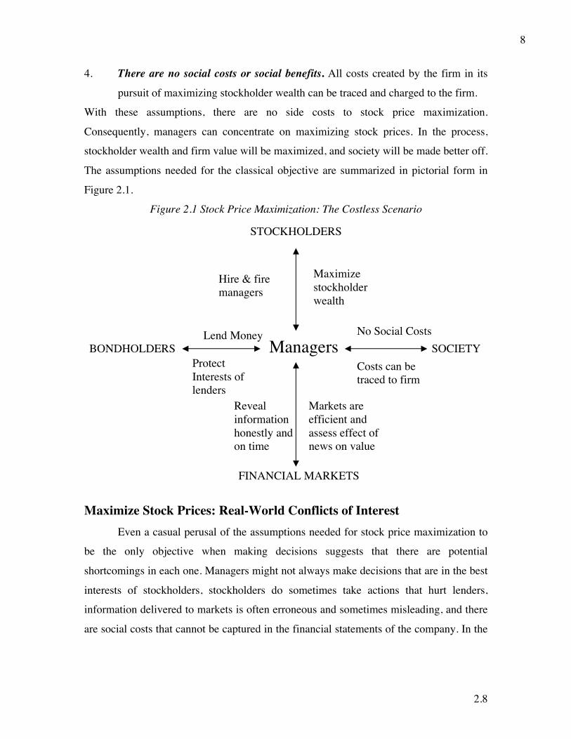
4. There are no social costs or social benefits. All costs created by the firm in its

pursuit of maximizing stockholder wealth can be traced and charged to the firm.

With these assumptions, there are no side costs to stock price maximization.

Consequently, managers can concentrate on maximizing stock prices. In the process,

stockholder wealth and firm value will be maximized, and society will be made better off.

The assumptions needed for the classical objective are summarized in pictorial form in

Figure 2.1.

Figure 2.1 Stock Price Maximization: The Costless Scenario

STOCKHOLDERS

Maximizestockholderwealth

Hire & firemanagers

BONDHOLDERSLend Money

ProtectInterests oflenders

FINANCIAL MARKETS

SOCIETYManagers

Revealinformationhonestly andon time

Markets areefficient andassess effect ofnews on value

No Social Costs

Costs can betraced to firm

Maximize Stock Prices: Real-World Conflicts of Interest Even a casual perusal of the assumptions needed for stock price maximization to

be the only objective when making decisions suggests that there are potential

shortcomings in each one. Managers might not always make decisions that are in the best

interests of stockholders, stockholders do sometimes take actions that hurt lenders,

information delivered to markets is often erroneous and sometimes misleading, and there

are social costs that cannot be captured in the financial statements of the company. In the

2.9

9

section that follows, we consider some of the ways real-world problems might trigger a

breakdown in the stock price maximization objective.

Stockholders and Managers

In classical corporate financial theory, stockholders are assumed to have the

power to discipline and replace managers who do not maximize their wealth. The two

mechanisms that exist for this power to be exercised are the annual meeting, wherein

stockholders gather to evaluate management performance, and the board of directors,

whose fiduciary duty it is to ensure that managers serve stockholders’ interests. Although

the legal backing for this assumption may be reasonable, the practical power of these

institutions to enforce stockholder control is debatable. In this section, we will begin by

looking at the limits on stockholder power and then examine the consequences for

managerial decisions.

The Annual Meeting

Every publicly traded firm has an annual meeting of its stockholders, during

which stockholders can both voice their views on management and vote on changes to the

corporate charter. Most stockholders, however, do not go to the annual meetings, partly

because they do not feel that they can make a difference and partly because it would not

make financial sense for them to do so.1 It is true that investors can exercise their power

with proxies,2 but incumbent management starts of with a clear advantage.3 Many

stockholders do not bother to fill out their proxies; among those who do, voting for

incumbent management is often the default option. For institutional stockholders with

significant holdings in a large number of securities, the easiest option, when dissatisfied

with incumbent management, is to “vote with their feet,” which is to sell their stock and

move on. An activist posture on the part of these stockholders would go a long way

1An investor who owns 100 shares of stock in, say, Coca-Cola will very quickly wipe out any potential returns he makes on his investment if he or she flies to Atlanta every year for the annual meeting. 2A proxy enables stockholders to vote in absentia on boards of directors and on resolutions that will be coming to a vote at the meeting. It does not allow them to ask open-ended questions of management. 3This advantage is magnified if the corporate charter allows incumbent management to vote proxies that were never sent back to the firm. This is the equivalent of having an election in which the incumbent gets the votes of anybody who does not show up at the ballot box.

2.10

10

toward making managers more responsive to their interests, and there are trends toward

more activism, which will be documented later in this chapter.

The Board of Directors

The board of directors is the body that oversees the management of a publicly

traded firm. As elected representatives of the stockholders, the directors are obligated to

ensure that managers are looking out for stockholder interests. They can change the top

management of the firm and have a substantial influence on how it is run. On major

decisions, such as acquisitions of other firms, managers have to get the approval of the

board before acting.

The capacity of the board of directors to discipline management and keep them

responsive to stockholders is diluted by a number of factors.

1. Many individuals who serve as directors do not spend much time on their fiduciary

duties, partly because of other commitments and partly because many of them serve

on the boards of several corporations. Korn/Ferry,4 an executive recruiter, publishes a

periodical survey of directorial compensation, and time spent by directors on their

work illustrates this very clearly. In their 1992 survey, they reported that the average

director spent 92 hours a year on board meetings and preparation in 1992, down from

108 in 1988, and was paid $32,352, up from $19,544 in 1988.5 As a result of scandals

associated with lack of board oversight and the passage of Sarbanes-Oxley, directors

have come under more pressure to take their jobs seriously. The Korn/Ferry survey

for 2007 noted an increase in hours worked by the average director to 192 hours a

year and a corresponding surge in compensation to $62,500 a year, an increase of

45% over the 2002 numbers.

2. Even those directors who spend time trying to understand the internal workings of a

firm are stymied by their lack of expertise on many issues, especially relating to

accounting rules and tender offers, and rely instead on outside experts.

4Korn/Ferry surveys the boards of large corporations and provides insight into their composition. 5This understates the true benefits received by the average director in a firm, because it does not count benefits and perquisites—insurance and pension benefits being the largest component. Hewitt Associates, an executive search firm, reports that 67 percent of 100 firms that they surveyed offer retirement plans for their directors.

2.11

11

3. In some firms, a significant percentage of the directors work for the firm, can be

categorized as insiders and are unlikely to challenge the chief executive office (CEO).

Even when directors are outsiders, they are often not independent, insofar as the

company’s CEO often has a major say in who serves on the board. Korn/Ferry’s

annual survey of boards also found in 1988 that 74 percent of the 426 companies it

surveyed relied on recommendations by the CEO to come up with new directors,

whereas only 16 percent used a search firm. In its 1998 survey, Korn/Ferry found a

shift toward more independence on this issue, with almost three-quarters of firms

reporting the existence of a nominating committee that is at least nominally

independent of the CEO. The latest Korn/Ferry survey confirmed a continuation of

this shift, with only 20% of directors being insiders and a surge in boards with

nominating committees that are independent of the CEO.

4. The CEOs of other companies are the favored choice for directors, leading to a

potential conflict of interest, where CEOs sit on each other’s boards. In the Korn-

Ferry survey, the former CEO of the company sits on the board at 30% of US

companies and 44% of French companies.

5. Many directors hold only small or token stakes in the equity of their corporations.

The remuneration they receive as directors vastly exceeds any returns that they make

on their stockholdings, thus making it unlikely that they will feel any empathy for

stockholders, if stock prices drop.

6. In many companies in the United States, the CEO chairs the board of directors

whereas in much of Europe, the chairman is an independent board member.

The net effect of these factors is that the board of directors often fails at its

assigned role, which is to protect the interests of stockholders. The CEO sets the agenda,

chairs the meeting, and controls the flow of information, and the search for consensus

generally overwhelms any attempts at confrontation. Although there is an impetus toward

reform, it has to be noted that these revolts were sparked not by board members but by

large institutional investors.

The failure of the board of directors to protect stockholders can be illustrated with

numerous examples from the United States, but this should not blind us to a more

troubling fact. Stockholders exercise more power over management in the United States

2.12

12

than in any other financial market. If the annual meeting and the board of directors are,

for the most part, ineffective in the United States at exercising control over management,

they are even more powerless in Europe and Asia as institutions that protect stockholders.

Ownership Structure

The power that stockholders have to influence management decisions either

directly (at the annual meeting) or indirectly (through the board of directors) can be

affected by how voting rights are apportioned across stockholders and by who owns the

shares in the company.

a. Voting rights: In the United States, the most common structure for voting rights in a

publicly traded company is to have a single class of shares, with each share getting a

vote. Increasingly, though, we are seeing companies like Google, News Corp and

Viacom, with two classes of shares with disproportionate voting rights assigned to

one class. In much of Latin America, shares with different voting rights are more the

rule than the exception, with almost every company having common shares (with

voting rights) and preferred shares (without voting rights). While there may be good

reasons for having share classes with different voting rights6, they clearly tilt the

scales in favor of incumbent managers (relative to stockholders), since insiders and

incumbents tend to hold the high voting right shares.

b. Founder/Owners: In young companies, it is not uncommon to find a significant

portion of the stock held by the founders or original promoters of the firm. Thus,

Larry Ellison, the founder of Oracle, continues to hold almost a quarter of the firm’s

stock and is also the company’s CEO. As small stockholders, we can draw solace

from the fact that the top manager in the firm is also its largest stockholder, but there

is still the danger that what is good for an inside stockholder with all or most of his

wealth invested in the company may not be in the best interests of outside

stockholders, especially if the latter are diversified across multiple investments.

c. Passive versus Active investors: As institutional investors increase their holdings of

equity, classifying investors into individual and institutional becomes a less useful

6 One argument is that stockholders in capital markets tend to be short term and that the investors who own the voting shares are long term. Consequently, entrusting the latter with the power will lead to better decisions.

2.13

13

exercise at many firms. There are, however, big differences between institutional

investors in terms of how much of a role they are willing to play in monitoring and

disciplining errant managers. Most institutional investors, including the bulk of

mutual and pension funds, are passive investors, insofar as their response to poor

management is to vote with their feet, by selling their stock. There are few

institutional investors, such as hedge funds and private equity funds, that have a much

more activist bent to their investing and seek to change the way companies are run.

The presence of these investors should therefore increase the power of all

stockholders, relative to managers, at companies.

d. Stockholders with competing interests: Not all stockholders are single minded about

maximizing stockholders wealth. For some stockholders, the pursuit of stockholder

wealth may have to be balanced against their other interests in the firm, with the

former being sacrificed for the latter. Consider two not uncommon examples. The

first is employees of the firm, investing in equity either directly or through their

pension fund. They have to balance their interests as stockholders against their

interests as employees. An employee layoff may help them as stockholders but work

against their interests, as employees. The second is that the government can be the

largest equity investor, which is often the aftermath of the privatization of a

government company. While governments want to see the values of their equity

stakes grow, like all other equity investors, they also have to balance this interest

against their other interests (as tax collectors and protectors of domestic interests).

They are unlikely to welcome plans to reduce taxes paid or to move production to

foreign locations.

e. Corporate Cross Holdings: The largest stockholder in a company may be another

company. In some cases, this investment may reflect strategic or operating

considerations. In others, though, these cross holdings are a device used by investors

or managers to wield power, often disproportionate to their ownership stake. Many

Asian corporate groups are structured as pyramids, with an individual or family at the

top of the pyramid controlling dozens of companies towards the bottom using

corporations to hold stock. In a slightly more benign version, groups of companies are

2.14

14

held together by companies holding stock in each other (cross holdings) and using

these cross holdings as a shield against stockholder challenges.

In summary, corporate governance is likely to be strongest in companies that have only

one class of shares, limited cross holdings and a large activist investor holding and

weakest in companies that have shares with different voting rights, extensive cross

holdings and/or a predominantly passive investor base.

In Practice: Corporate governance at companies

The modern publicly traded corporation is a case study in conflicts of interest,

with major decisions being made by managers whose interests may diverge from those of

stockholders. Put simply, corporate governance as a sub-area in finance looks at the

question of how best to monitor and motivate managers to behave in the best interests of

the owners of the company (stockholders). In this context, a company where managers

are entrenched and cannot be removed even if they make bad decisions (which hut

stockholders) is one with poor corporate governance.

In the light of accounting scandals and faced with opaque financial statements, it

is clear investors care more today about corporate governance at companies and

companies know that they do. In response to this concern, firms have expended resources

and a large portion of their annual reports to conveying to investors their views on

corporate governance (and the actions that they are taking to improve it). Many

companies have made explicit the corporate governance principles that govern how they

choose and remunerate directors. In the case of Disney, these principles, which were first

initiated a few years ago, have been progressively strengthened over time and the October

2008 version requires a substantial majority of the directors to be independent and own at

least $100,000 worth of stock.

The demand from investors for unbiased and objective corporate governance

scores has created a business for third parties that try to assess corporate governance at

individual firms. In late 2002, Standard and Poor’s introduced a corporate governance

score that ranged from 1 (lowest) to 10 (higher) for individual companies, based upon

weighting a number of factors including board composition, ownership structure and

financial structure. The Corporate Library, an independent research group started by

stockholder activists, Neil Minow and Robert Monks, tracks and rates the effectiveness of

2.15

15

boards. Institutional Shareholder Service (ISS), a proxy advisory firm, rates more than

8000 companies on a number of proprietary dimensions and markets its Corporate

Governance Quotient (CGQ) to institutional investors. There are other entities that now

offer corporate governance scores for European companies and Canadian companies.

The Consequences of Stockholder Powerlessness

If the two institutions of corporate governance—annual meetings and the board of

directors—fail to keep management responsive to stockholders, as argued in the previous

section, we cannot expect managers to maximize stockholder wealth, especially when

their interests conflict with those of stockholders. Consider the following examples.

1. Fighting Hostile Acquisitions

When a firm is the target of a hostile takeover, managers are sometimes faced with an

uncomfortable choice. Allowing the hostile acquisition to go through will allow

stockholders to reap substantial financial gains but may result in the managers losing

their jobs. Not surprisingly, managers often act to protect their own interests at the

expense of stockholders:

• The managers of some firms that were targeted by

acquirers (raiders) for hostile takeovers in the 1980s

were able to avoid being acquired by buying out the

acquirer’s existing stake, generally at a price much

greater than the price paid by the acquirer and by

using stockholder cash. This process, called

greenmail, usually causes stock prices to drop, but it

does protect the jobs of incumbent managers. The irony of using money that

belongs to stockholders to protect them against receiving a higher price on the

stock they own seems to be lost on the perpetrators of greenmail.

• Another widely used anti-takeover device is a golden parachute, a provision in an

employment contract that allow for the payment of a lump-sum or cash flows over

a period, if the manager covered by the contract loses his or her job in a takeover.

Although there are economists who have justified the payment of golden

parachutes as a way of reducing the conflict between stockholders and managers,

Greenmail: Greenmail refers to

the purchase of a potential

hostile acquirer’s stake in a

business at a premium over the

price paid for that stake by the

target company.

2.16

16

it is still unseemly that managers should need large side payments to do what they

are hired to do—maximize stockholder wealth.

• Firms sometimes create poison pills, which are triggered by hostile takeovers. The

objective is to make it difficult and costly to acquire control. A flip over right

offers a simple example. In a flip over right, existing stockholders get the right to

buy shares in the firm at a price well above

the current stock price. As long as the

existing management runs the firm; this

right is not worth very much. If a hostile

acquirer takes over the firm, though,

stockholders are given the right to buy

additional shares at a price much lower

than the current stock price. The acquirer, having weighed in this additional cost,

may very well decide against the acquisition.

Greenmail, golden parachutes, and poison pills generally do not require stockholder

approval and are usually adopted by compliant boards of directors. In all three cases, it

can be argued, managerial interests are being

served at the expenses of stockholder interests.

2. Antitakeover Amendments

Antitakeover amendments have the same

objective as greenmail and poison pills, which is dissuading hostile takeovers, but differ

on one very important count. They require the assent of stockholders to be instituted.

There are several types of antitakeover amendments, all designed with the objective of

reducing the likelihood of a hostile takeover. Consider, for instance, a super-majority

amendment; to take over a firm that adopts this amendment, an acquirer has to acquire

more than the 51 percent that would normally be required to gain control. Antitakeover

amendments do increase the bargaining power of managers when negotiating with

acquirers and could work to the benefit of stockholders, but only if managers act in the

best interests of stockholders.

2.2.: Anti-takeover Amendments and Management Trust

Golden Parachute: A golden parachute refers

to a contractual clause in a management

contract that allows the manager to be paid a

specified sum of money in the event control of

the firm changes, usually in the context of a

hostile takeover.

Poison Pill: A poison pill is a security or a

provision that is triggered by the hostile

acquisition of the firm, resulting in a large

cost to the acquirer.

2.17

17

If as a stockholder in a company, you were asked to vote on an amendment to the

corporate charter that would restrict hostile takeovers of your company and give your

management more power, in which of the following types of companies would you be

most likely to vote yes to the amendment?

a. Companies where the managers promise to use this power to extract a higher price for

you from hostile bidders.

b. Companies that have done badly (in earnings and stock price performance) in the past

few years.

c. Companies that have done well (in earnings and stock price performance) in the past

few years.

d. I would never vote for such an amendment.

3. Paying too Much on Acquisitions

There are many ways in which managers can make

their stockholders worse off—by investing in bad

projects, by borrowing too much or too little, and by

adopting defensive mechanisms against potentially

value-increasing takeovers. The quickest and perhaps

the most decisive way to impoverish stockholders is to

overpay on a takeover, because the amounts paid on

takeovers tend to dwarf those involved in the other decisions. Of course, the managers of

the firms doing the acquiring will argue that they never overpay on takeovers, 7 and that

the high premiums paid in acquisitions can be justified using any number of reasons—

there is synergy, there are strategic considerations, the target firm is undervalued and

badly managed, and so on. The stockholders in acquiring firms do not seem to share the

enthusiasm for mergers and acquisitions that their managers have, because the stock

prices of bidding firms decline on the takeover announcements a significant proportion of

the time.8

7One explanation given for the phenomenon of overpaying on takeovers is that it is managerial hubris (pride) that drives the process. 8See Jarrell, G.A., J.A. Brickley and J.M. Netter, 1988, The Market for Corporate Control: The Empirical Evidence since 1980, Journal of Economic Perspectives, Vol 2, 49-68.. In an extensive study of returns to

Synergy: Synergy is the additional value

created by bringing together two entities

and pooling their strengths. In the

context of a merger, synergy is the

difference between the value of the

merged firm and sum of the values of the

firms operating independently.

2.18

18

These illustrations are not meant to make the case that managers are venal and

selfish, which would be an unfair charge, but are manifestations of a much more

fundamental problem; when there is conflict of interest between stockholders and

managers, stockholder wealth maximization is likely to take second place to management

objectives.

The Imperial CEO and Compliant Directors: A Behavioral Perspective

Many corporate fiascos would be avoided or at least made less damaging if

independent directors asked tough questions and reined in top managers. Given this

reality, an interesting question is why we do not see this defiance more often in practice.

Some of the failures of boards to restrain CEOs can be attributed to institutional factors

and board selection processes, but some can be attributed to human frailties.

Studies of social psychology have noted that loyalty is hardwired into human

behavior. While this loyalty is an important tool in building up organizations, it can also

lead people to suppress internal ethical standards if they conflict with loyalty to an

authority figure. In a famous experiment illustrating this phenomenon, Stanley Milgram,

a psychology professor at Yale, asked students to electrocute complete strangers who

gave incorrect answers to questions, with larger shocks for more subsequent erroneous

answers. Milgram expected his students to stop, when they observed the strangers (who

were actors) in pain, but was horrified to find that students continued to shock subjects, if

ordered to do so by an authority figure. In the context of corporate governance, directors

remain steadfastly loyal to the CEO, even in the face of poor performance or bad

decisions, and this loyalty seems to outweigh their legal responsibilities to stockholders,

who are not present in the room.

How can we break this genetic predisposition to loyalty? The same psychological

studies that chronicle loyalty to authority figures also provide guidance on factors that

weaken that loyalty. The first is the introduction of dissenting peers; if some people are

observed voicing opposition to authority, it increases the propensity of others to do the

bidder firms, these authors note that excess returns on these firms’ stocks around the announcement of takeovers have declined from an average of 4.95 percent in the 1960s to 2 percent in the 1970s to –1 percent in the 1980s. Studies of mergers also generally conclude that the stock prices of bidding firms decline in more than half of all acquisitions.

2.19

19

same. The second is the existence of discordant authority figures, and disagreement

among these figures; in the Milgram experiments, having two people dressed identically

in lab coats disagreeing about directions, reduced obedience significantly. If we take

these findings to heart, we should not only aspire to increase the number of independent

directors on boards, but also allow these directors to be nominated by the shareholders

who disagree most with incumbent managers. In addition, the presence of a non-

executive as Chairman of the board and lead independent directors may allow for a

counter-weight to the CEO in board meetings.

Even with these reforms, we have to accept the reality that boards of directors will

never be as independent nor as probing as we would like them to be, for two other

reasons. The first is that people tend to go along with a group consensus, even if that

consensus is wrong. To the extent that CEOs frame the issues at board meetings, this

consensus is likely to work in their favor. The second comes from work done on

information cascades, where people imitate someone they view to be an informed player,

rather than pay to become informed themselves. If executive or inside directors are

viewed as more informed about the issues facing the board, it is entirely likely that the

outside directors, even if independent, will go along with their views. One solution,

offered by Randall Morck, and modeled after the Catholic Church is to create a Devil’s

advocate, a powerful counter-authority to the CEO, whose primary role is to oppose and

critique proposed strategies and actions.9

Illustration 2.1 Assessing Disney’s Corporate Governance

To understand how corporate governance has evolved at Disney, we have to look

at its history. For much of its early existence, Disney was a creation of its founder, Walt

Disney. His vision and imagination were the genesis for the animated movies and theme

parks that made the company’s reputation. After Walt’s demise in 1966, Disney went

through a period of decline, where its movies failed at the box office and attendance at

theme parks crested. In 1984, Michael Eisner, then an executive at Paramount, was hired

as CEO for Disney. Over the next decade, Eisner succeeded in regenerating Disney, with

9 Morck, R., 2004, Behavioral Finance in Corporate Governance – Independent Directors, Non-executive Chairs and the Importance of the Devil’s Advocate, NBER Working Paper series.

2.20

20

his protégé, Jeffrey Katzenberg, at the head of the animated movie division, producing

blockbuster hits including The Little Mermaid, Beauty and the Beast and The Lion

King.10

As Disney’s earnings and stock price increased, Eisner’s power also amplified

and by the mid 1990s, he had brought together a board of directors that genuflected to

that power. In 1996, Fortune magazine ranked Disney as having the worst board of the

Fortune 500 companies, and the 16 members on its board and the members are listed in

Table 2.1, categorized by whether they worked for Disney (insiders) or not (outsiders).

Table 2.1 Disney’s Board of Directors 1996

Insiders Outsiders 1. Michael D. Eisner: CEO 2. Roy E. Disney: Head of animation

department 3. Sanford M. Litvack: Chief of corporate

operations 4. Richard A. Nunis: Chairman of Walt

Disney Attractions 5. *Raymond L. Watson,: Disney

chairman in 1983 and 1984 6. *E. Cardon Walker: Disney chairman

and chief executive, 1980–83 7. *Gary L. Wilson: Disney chief

financial officer, 1985–89 8. *Thomas S. Murphy: Former chairman

and chief executive of Capital Cities/ABC Inc.

*Former officials of Disney

1. Reveta F. Bowers: Head of school for the Center for Early Education, where Mr. Eisner’s children attended class

2. Ignacio E. Lozano Jr.,: Chairman of Lozano Enterprises, publisher of La Opinion newspaper in Los Angeles

3. George J. Mitchell: Washington, D.C. attorney, former U.S. senator. Disney paid Mr. Mitchell $50,000 for his consulting on international business matters in 1996. His Washington law firm was paid an additional $122,764

4. Stanley P. Gold: President and chief executive of Shamrock Holdings, Inc., which manages about $1 billion in investments for the Disney family

5. The Rev. Leo J. O’Donovan: President of Georgetown University, where one of Mr. Eisner’s children attended college. Mr. Eisner sat on the Georgetown board and has contributed more than $1 million to the school

6. Irwin E. Russell: Beverly Hills, Calif., attorney whose clients include Mr. Eisner

7. *Sidney Poitier: Actor. 8. Robert A. M. Stern: New York

architect who has designed numerous

10 For an exceptionally entertaining and enlightening read, we would suggest the book “Disney Wars”, authored by Michael Lewis. The book tracks Michael Eisner’s tenure at Disney and how his strengths ultimately became his weakest links.

2.21

21

Disney projects. He received $168,278 for those services in fiscal year 1996

Note that eight of the sixteen members on the board were current or ex Disney employees

and that Eisner, in addition to being CEO, chaired the board. Of the eight outsiders, at

least five had potential conflicts of interests because of their ties with either Disney or

Eisner. The potential conflicts are listed in italics in Table 2.1. Given the composition of

this board, it should come as no surprise that it failed to assert its power against

incumbent management.11 In 1997, CALPERS, the California Public Employees

Retirement System, suggested a series of checks to see if a board was likely to be

effective in acting as a counterweight to a powerful CEO, including:

• Are a majority of the directors outside directors?

• Is the chairman of the board independent of the company (and not the CEO of the

company)?

• Are the compensation and audit committees composed entirely of outsiders?

When CALPERS put the companies in the Standard & Poor’s (S&P) 500 through these

tests in 1997, Disney was the only company that failed all three tests, with insiders on

every one of the key committees.

Disney came under pressure from stockholders to modify its corporate

governance practices between 1997 and 2002 and made some changes to its corporate

governance practices. By 2002, the number of insiders on the board had dropped to four,

but it remained unwieldy (with 16 board members) and had only limited effectiveness. In

2003, two board members, Roy Disney and Stanley Gold, resigned from the board,

complaining that it was too willing to rubber stamp Michael Eisner’s decisions. At the

2004 annual meeting, an unprecedented 43% of shareholders withheld their proxies when

asked to re-elect Eisner to the board. In response, Eisner stepped down as chairman of the

board in 2004 and finally as CEO in March 2005. His replacement, Bob Iger, has shown

more signs of being responsive to stockholders. At the end of 2008, Disney’s board of

directors had twelve members, only one of whom (Bob Iger) was an insider.

11One case that cost Disney dearly was when Eisner prevailed on the board to hire Michael Ovitz, a noted Hollywood agent, with a generous compensation. A few years later, Ovitz left the company after falling out with Eisner, creating a multimillion-dollar liability for Disney. A 2003 lawsuit against Disney’s board

2.22

22

Table 2.2 Disney’s Board of Directors 2008

Board Members Occupation

John E. Pepper, Jr. (Chairman)

Retired Chairman and CEO, Procter & Gamble Co.

Susan E. Arnold President, Global Business Units, Procter & Gamble Co. John E. Bryson Retired Chairman and CEO, Edison International John S. Chen Chairman,, CEO & President, Sybase, Inc. Judith L. Estrin CEO, JLabs,  LLC.  Robert A. Iger CEO, Disney Steven P. Jobs CEO, Apple Fred Langhammer Chairman, Global Affairs, The Estee Lauder Companies Aylwin B. Lewis President and CEO, Potbelly Sandwich Works Monica Lozano Publisher and CEO, La Opinion Robert W. Matschullat Retired Vice Chairman and CFO, The Seagram Co. Orin C. Smith Retired President and CEO, Starbucks Corporation

At least in terms of appearances, this board looks more independent than the Disney

boards of earlier years, with no obvious conflicts of interest. There are two other

interesting shifts. The first is that there are only four board members from 2003 (the last

Eisner board), who continue on this one, an indication that this is now Iger’s board of

directors. The other is the presence of Steve Jobs on the list. While his expertise in

technology is undoubtedly welcome to the rest of the board members, he also happens to

be Disney’s largest stockholder, owning in excess of 6% of the company.12 Disney

stockholders may finally have someone who will advocate for their interests in board

deliberations. External monitors who track corporate governance have noticed the

improvement at Disney. At the start of 2009, ISS ranked Disney first among media

companies on its corporate governance score (CGQ) and among the top 10 firms in the

S&P 500, a remarkable turnaround for a firm that was a poster child for bad corporate

governance only a few years ago.

Illustration 2.2 Corporate Governance at Aracruz: Voting and Nonvoting Shares

Aracruz Cellulose, like most Brazilian companies, had two classes of shares at the

end of 2008. The common shares had all of the voting rights and were held by incumbent

members contended that they failed in their fiduciary duty by not checking the terms of the compensation agreement before assenting to the hiring.

2.23

23

management, lenders to the company, and the Brazilian government. Outside investors

held the nonvoting shares, which were called preferred shares,13 and had no say in the

election of the board of directors. At the end of 2008, Aracruz was managed by a board

of seven directors, composed primarily of representatives of those who own the common

(voting) shares, and an executive board, composed of three managers of the company.

Without analyzing the composition of the board of Aracruz, it is quite clear that

there is the potential for a conflict of interest between voting shareholders who are fully

represented on the board and preferred stockholders who are not. Although Brazilian law

provides some protection for the latter, preferred stockholders have no power to change

the existing management of the company and have little influence over major decisions

that can affect their value.14 As a more general proposition, the very existence of voting

and non-voting shares can be viewed as an indication of poor corporate governance, even

at companies like Google that are viewed as well managed companies.

Illustration 2.3 Corporate Governance at Deutsche Bank: Two Boards?

Deutsche Bank follows the German tradition and legal requirement of having two

boards. The board of managing directors, composed primarily of incumbent managers,

develops the company’s strategy, reviews it with the supervisory board, and ensures its

implementation. The supervisory board appoints and recalls the members of the board of

managing directors and, in cooperation with that board, arranges for long-term successor

planning. It also advises the board of managing directors on the management of business

and supervises it in its achievement of long-term goals.

A look at the supervisory board of directors at Deutsche Bank provides some

insight into the differences between the U.S. and German corporate governance systems.

The supervisory board at Deutsche Bank consists of twenty members, but eight are

representatives of the employees. The remaining twelve are elected by shareholders, but

12 This holding can be traced back to the large ownership stake that Steve Jobs had in Pixar. When Pixar was acquired by Disney, Jobs received shares in Disney in exchange for this holding. 13This can create some confusion for investors in the United States, where preferred stock is stock with a fixed dividend and resembles bonds more than conventional common stock. 14 This was brought home when Ambev, a large Brazilian beverage company, was acquired by Interbrand, a Belgian corporation. The deal enriched the common stock holders but the preferred stockholders received little in terms of a premium and were largely bystanders.

2.24

24

employees clearly have a much bigger say in how companies are run in Germany and can

sometimes exercise veto power over company decisions.

Illustration 2.4 Corporate Governance at Tata Chemicals: Family Group Companies

As we noted in chapter 1, Tata Chemicals is part of the Tata Group of companies,

one of India’s largest family group companies. In 2009, the company had eight directors,

four of whom could be categorized as insiders and four as independent.15 The chairman

of the board, Ratan Tata, also operates as the chairman of the boards of 12 other Tata

companies. In fact, many of the directors on the board of Tata Chemicals serve on the

boards of other Tata companies as well. The intermingling of group and company

interests is made even greater by the fact that other Tata group companies own 29.15% of

the outstanding shares in Tata Chemicals and Tata Chemicals has significant investments

in other Tata companies.

As stockholders in Tata Chemicals, there are two key implications for corporate

governance:

1. Limited power: The large cross holdings by group companies makes it unlikely that

individual investors (who are not members of the Tata family) will be able to exercise

much power at any of these companies.

2. Conflict of interest: The conflict between what is good for the investors in the

company (Tata Chemicals) and what is good for the group (Tata group) will play out

on almost every major corporate finance decision. For instance, when it comes to how

much Tata Chemicals should pay in dividends, the key determinant may not be how

much the company generates in excess cash but how much funding is needed by other

companies in the group. Generalizing, decisions that are made with the best interests

of the Tata group may be hurtful or costly to investors in Tata Chemicals.

Note that this is not a critique directed specifically at the Tata Group. In fact, many

investors who follow Indian companies view the Tata Group as one of the more

enlightened family businesses in India. It is a more general problem with investing in a

company that belongs to a larger group, since group interests may render waste to the

interests of investors in individual companies.

2.25

25

In Practice: Is There a Payoff to Better Corporate Governance?

We do not want to oversell the importance of strong corporate governance. It is

not a magic bullet that will somehow make bad managers into good managers. In fact, we

can visualize a well-managed company with poor corporate governance just as easily as

we can see a poorly managed company with good corporate governance. The biggest pay

off to good corporate governance is that it is far easier to replace bad managers at a firm,

thus making long term mismanagement less likely.

Academics and activist investors are understandably enthused by moves toward

giving stockholders more power over managers, but a practical question that is often not

answered is what the payoff to better corporate governance is. Are companies where

stockholders have more power over managers managed better and run more efficiently?

If so, are they more valuable? Although no individual study can answer these significant

questions, there are a number of different strands of research that offer some insight:

• In the most comprehensive study of the effect of corporate governance on value, a

governance index was created for each of 1500 firms based on 24 distinct

corporate governance provisions.16 Buying stocks that had the strongest investor

protections while simultaneously selling shares with the weakest protections

generated an annual excess return of 8.5 percent. Every one-point increase in the

index toward fewer investor protections decreased market value by 8.9 percent in

1999, and firms that scored high in investor protections also had higher profits,

higher sales growth, and made fewer acquisitions. These findings are echoed in

studies on firms in Korea and Germany. 17 The recent studies are more nuanced in

their findings. While most continue to find a link between corporate governance

scores and market pricing (such as price to book ratios), they find little

relationship between operating performance measures (profit margins, returns on

equity) and these scores.

15 Two of the directors are categorized as promoters, a term that indicates that they are either founders or descendants of the founders of these firms. 16Gompers, P. A., J. L. Ishii, and A. Metrick, 2003, “Corporate Governance and Equity Prices,” Quarterly Journal of Economics, 118, 107–155. The data for the governance index was obtained from the Investor Responsibility Research Center, which tracks the corporate charter provisions for hundreds of firms.

2.26

26

• Actions that restrict hostile takeovers generally reduce stockholder power by

taking away one of the most potent weapons available against indifferent

management. In 1990, Pennsylvania considered passing a state law that would

have protected incumbent managers against hostile takeovers by allowing them to

override stockholder interests if other stakeholders were adversely impacted. In

the months between the time the law was first proposed and the time it was

passed, the stock prices of Pennsylvania companies declined by 6.90 percent.18

• There seems to be little evidence of a link between the composition of the board

of directors and firm value. In other words, there is little to indicate that

companies with boards that have more independent directors trade at higher prices

than companies with insider-dominated boards.19

• Although this is anecdotal evidence, the wave of corporate scandals indicates a

significant cost to having a compliant board. A common theme that emerges at

problem companies is an ineffective board that failed to ask tough questions of an

imperial CEO. The banking crisis of 2008, for instance, revealed that the boards

of directors at investment banks were not only unaware of the risks of the

investments made at these banks, but had few tools for overseeing or managing

that risk.

In closing, stronger corporate governance is not a panacea for all our troubles. However,

it does offer the hope of change, especially when incumbent managers fail to do their

jobs.

Stockholders and Bondholders

In a world where what is good for stockholders in a firm is also good for its

bondholders (lenders), the latter might not have to worry about protecting themselves

from expropriation. In the real world, however, there is a risk that bondholders who do

not protect themselves may be taken advantage of in a variety of ways—by stockholders

17For Korea: Black, B S., H. Jang, and W. Kim, 2003, Does Corporate Governance Affect Firm Value? Evidence from Korea, Stanford Law School Working Paper. For Germany: Drobetz, W., 2003, Corporate Governance: Legal Fiction or Economic Reality, Working Paper, University of Basel. 18Karpoff, J. M. and P. H. Malatesta, 1990, “The Wealth Effects of Second-Generation State Takeover Legislation,” Journal of Financial Economics, 25, 291–322.

2.27

27

borrowing more money, paying more dividends, or undercutting the security of the assets

on which the loans were based.

The Source of the Conflict

The source of the conflict of interest

between stockholders and bondholders lies in the

differences in the nature of the cash flow claims of

the two groups. Bondholders generally have first

claim on cash flows but receive fixed interest

payments, assuming that the firm makes enough

income to meet its debt obligations. Equity

investors have a claim on the cash flows that are left over but have the option in publicly

traded firms of declaring bankruptcy if the firm has insufficient cash flows to meet its

financial obligations. Bondholders do not get to participate on the upside if the projects

succeed but bear a significant portion of the cost if they fail. As a consequence,

bondholders tend to view the risk in investments much more negatively than

stockholders. There are many issues on which stockholders and bondholders are likely to

disagree.

Some Examples of the Conflict

Existing bondholders can be made worse off by increases in borrowing, especially

if these increases are large and affect the default risk of the firm, and these bondholders

are unprotected. The stockholders’ wealth increases concurrently. This effect is

dramatically illustrated in the case of acquisitions funded primarily with debt, where the

debt ratio increases and the bond rating drops significantly. The prices of existing bonds

fall to reflect the higher default risk.20

Dividend policy is another issue on which a conflict of interest may arise between

stockholders and bondholders. The effect of higher dividends on stock prices can be

debated in theory, with differences of opinion on whether it should increase or decrease

19Bhagat, Sanjai and Bernard Black, 1999, “The Uncertain Relationship between Board Composition and Firm Performance,” Business Lawyer, 54, 921–963. 20In the leveraged buyout of Nabisco, existing bonds dropped in price 19 percent on the day of the acquisition, even as stock prices zoomed up.

Bond Covenants: Covenants are restrictions built

into contractual agreements. The most common

reference in corporate finance to covenants is in

bond agreements, and they represent restrictions

placed by lenders on investment, financing, and

dividend decisions made by the firm.

2.28

28

prices, but the empirical evidence is clear. Increases in dividends, on average, lead to

higher stock prices, whereas decreases in dividends lead to lower stock prices. Bond

prices, on the other hand, react negatively to dividend increases and positively to

dividend cuts. The reason is simple. Dividend payments reduce the cash available to a

firm, thus making debt more risky.

The Consequences of Stockholder–Bondholder Conflicts

As these two illustrations make clear, stockholders and bondholders have

different objectives and some decisions can transfer wealth from one group (usually

bondholders) to the other (usually stockholders). Focusing on maximizing stockholder

wealth may result in stockholders taking perverse actions that harm the overall firm but

increase their wealth at the expense of bondholders.

It is possible that we are making too much of the expropriation possibility, for a

couple of reasons. Bondholders are aware of the potential of stockholders to take actions

that are inimical to their interests and generally protect themselves, either by writing in

covenants or restrictions on what stockholders can do, or by taking an equity interest in

the firm. Furthermore, the need to return to the bond markets to raise further funds in the

future will keep many firms honest, because the gains from any one-time wealth transfer

are likely to by outweighed by the reputation loss associated with such actions. These

issues will be considered in more detail later in this book.

The Firm and Financial Markets There is an advantage to maintaining an objective that focuses on stockholder or

firm wealth rather than stock prices or the market value of the firm, because it does not

require any assumptions about the efficiency or otherwise of financial markets. The

downside, however, is that stockholder or firm wealth is not easily measurable, making it

difficult to establish clear standards for success and failure. It is true that there are

valuation models, some of which we will examine in this book, that attempt to measure

equity and firm value, but they are based on a large number of essentially subjective

inputs on which people may disagree. Because an essential characteristic of a good

objective is that it comes with a clear and unambiguous measurement mechanism, the

advantages of shifting to an objective that focuses on market prices is obvious. The

2.29

29

measure of success or failure is there for all to see. Successful managers raise their firms’

stock prices; unsuccessful managers reduce theirs.

The trouble with market prices is that the investors who assess them can make

serious mistakes. To the extent that financial markets are efficient and use the

information that is available to make measured and unbiased estimates of future cash

flows and risk, market prices will reflect true value. In such markets, both the measurers

and the measured will accept the market price as the appropriate mechanism for judging

success and failure.

There are two potential barriers to this. The first is that information is the

lubricant that enables markets to be efficient. To the extent that this information is

hidden, delayed, or misleading, market prices will deviate from true value, even in an

otherwise efficient market. The second problem is that there are many, both in academia

and in practice, who argue that markets are not efficient, even when information is freely

available. In both cases, decisions that maximize stock prices may not be consistent with

long-term value maximization.

2.3.: The Credibility of Firms in Conveying Information Do you think that the information revealed by companies about themselves is usually

timely and honest?

a. biased?

b. fraudulent?

The Information Problem

Market prices are based on information,

both public and private. In the world of classical

theory, information about companies is revealed

promptly and truthfully to financial markets. In the

real world, there are a few impediments to this

process. The first is that information is sometimes

suppressed or delayed by firms, especially when it

contains bad news. Although there is significant anecdotal evidence of this occurrence,

the most direct evidence that firms do this comes from studies of earnings and dividend

Public and Private Information: Public

information refers to any information that

is available to the investing public, whereas

private information is restricted to only

insiders or a few investors in the firm.

2.30

30

announcements. A study of earnings announcements noted that those announcements that

had the worst news tended to be delayed the longest, relative to the expected

announcement date.21 In a similar vein, a study of earnings and dividend announcements

by day of the week for firms on the New York Stock Exchange between 1982 and 1986

found that the announcements made on Friday, especially after the close of trading,

contained more bad news than announcements made on any other day of the week.22 This

suggests that managers try to release bad news when markets are least active or closed

because they fear that markets will overreact.

The second problem is more serious. In their zeal to keep investors happy and

raise market prices, some firms release intentionally misleading information about

current conditions and future prospects to financial markets. These misrepresentations

can cause stock prices to deviate significantly from value. Consider the example of Bre-

X, a Canadian gold mining company that claimed to have found one of the largest gold

reserves in the world in Indonesia in the early 1990s. The stock was heavily touted by

equity research analysts in the United States and Canada, but the entire claim was

fraudulent. When the fraud came to light in 1997, the stock price tumbled, and analysts

professed to be shocked that they had been misled by the firm. The implications of such

fraudulent behavior for corporate finance can be profound because managers are often

evaluated on the basis of stock price performance. Thus Bre-X managers with options or

bonus plans tied to the stock price probably did very well before the fraud came to light.

Repeated violations of investor trust by companies can also lead to a loss of faith in

equity markets and a decline in stock prices for all firms. Again, the potential for

information distortions is greater in emerging markers, where information disclosure laws

and corporate governance are both weaker. In 2008, the CEO and top management of

Satyam Computers, a well-regarded Indian software company, stepped down after

admitting to accounting fraud.23

21Penman, S. H., 1987, “The Distribution of Earnings News over Time and Seasonalities in Aggregate Stock Returns,” Journal of Financial Economics, 18(2), 199–228. 22Damodaran, A., 1989, “The Weekend Effect in Information Releases: A Study of Earnings and Dividend Announcements,” Review of Financial Studies, 2(4), 607–623. 23 To illustrate the pervasiveness of the misstatements in the financial statements, the cash balance that was reported on the balance sheet did not exist.

2.31

31

2.4. Reputation and Market Access Which of the following types of firms is more likely to mislead markets? Explain.

a. Companies that access markets infrequently to raise funds for operations—they raise

funds internally.

b. Companies that access markets frequently to raise funds for operations.

Explain.

The Market Problem

The fear that managers have of markets overreacting or not assimilating

information well into prices may be justified. Even if information flowed freely and with

no distortion to financial markets, there is no guarantee that what emerges as the market

price will be an unbiased estimate of true value. In fact, many would argue that the fault

lies deeper and that investors are much too irrational and unreliable to come up with a

good estimate of the true value. Some of the criticisms that have been mounted against

financial markets are legitimate, some are overblown, and some are simply wrong, but we

will consider all of them.

1. Financial markets do not always reasonably and rationally assess the effects of

new information on prices. Critics using this argument note that markets can be

volatile, reacting to no news at all in some cases; in any case, the volatility in

market prices is usually much greater than the volatility in any of the underlying

fundamentals. The argument that financial markets are much too volatile, given

he underlying fundamentals, has some empirical support.24 As for the irrationality

of markets, the frequency with which you see bubbles in markets from the tulip

bulb mania of the 1600s in Holland to the dot-com debacle of the late 1990s

seems to be proof enough that emotions sometime get ahead of reason in markets.

2. Financial markets sometimes over react to information. Analysts with this point

of view point to firms that reports earnings that are much higher or much lower

than expected and argue that stock prices jump too much on good news and drop

too much on bad news. The evidence on this proposition is mixed, though,

because there are other cases where markets seem to under react to news about

2.32

32

firms. Overall, the only conclusion that all these studies agree on is that markets

make mistakes in assessing the effect of news on value.

3. There are cases where insiders move markets to their benefit and often at the

expense of outside investors. This is especially true with illiquid stocks and is

exacerbated in markets where trading is infrequent. Even with widely held and

traded stocks, insiders sometimes use their superior access to information to get

ahead of other investors.25

Notwithstanding these limitations, we cannot take away from the central contribution of

financial markets. They assimilate and aggregate a remarkable amount of information on

current conditions and future prospects into one measure—the price. No competing

measure comes close to providing as timely or as comprehensive a measure of a firm’s

standing. The value of having market prices is best illustrated when working with a

private firm as opposed to a public firm. Although managers of the latter may resent the

second-guessing of analysts and investors, there is a great deal of value to knowing how

investors perceive the actions that the firm takes.

Irrational Exuberance: A Behavioral Perspective on Markets

The belief in efficient markets, long an article of faith in academic finance, has

come under assault from within the academy. The notion that markets make systematic

mistakes and fail to reflect true value often is now backed up not only by evidence but

has also been linked to well documented quirks in human nature. In a survey article on

the topic, Barberis and Thaler list the following characteristics that skew investor

behavior:26

a. Overconfidence: Investors are over confident in their own judgments, as evidenced by

their inability to estimate confidence intervals for quantities (such as the level of the

Dow) and probabilities of event occurring.

24Shiller , R. J., 2000, Irrational Exuberance, Princeton: Princeton University Press. 25This is true even in the presence of strong insider trading laws, as is the case in the United States. Studies that look at insider trades registered with the Securities and Exchange Commission (SEC) seem to indicate that insider buying and selling does precede stock prices going up and down, respectively. The advantage is small, though. 26 Barberis, N. and R. Thaler, 2002, A Survey of Behavioral Finance, NBER Working Paper.

2.33

33

b. Optimism and Wishful Thinking: Individuals have unrealistically optimistic views of

their own capabilities. For instance, 90% of people, when characterizing their own

skills, describe themselves as above average.

c. Representativeness: Individuals show systematic biases in how they classify data and

evaluate. One manifestation of this bias is that they ignore sample sizes, when

judging likelihood, treating a 60% success rate in a sample of 10 and the same

success rate in a sample of 1000 equivalently, even though the latter should convey

more information.

d. Conservatism and Belief Perseverance: Individuals seem to attach to much weight to

their prior beliefs about data and to not react sufficiently to new information. Once

they form an opinion, they are reluctant to search for evidence that may contradict

that opinion and when faced with such evidence, they view it with excessive

skepticism. In some cases, in what is called the confirmation bias, they actually look

at contradictory evidence as supportive of their beliefs.

e. Anchoring: When forming estimates, individuals start with an initial and often

arbitrary value and adjust this value insufficiently.

f. Availability biases: When assessing the likelihood of an event, individuals looking for

relevant information often overweight more recent events and events that affect them

personally more than they should in making their judgments.

Given that these characteristics are widespread and perhaps universal, we should not be

surprised that markets reflect them. The overconfidence and over optimism feed into

price bubbles in individual stocks as well as the entire market, and those who question the

rationality of the bubbles are often ignored (belief perseverance). Anchoring and

availability biases can skew how we value individual companies, again leading to

significant differences between market prices and true values. In general, behavioral

finance provides explanations for why stock prices may deviate from true value for

extended periods.

2.5. Are Markets Short-Term?

2.34

34

Focusing on market prices will lead companies toward short-term decisions at the

expense of long-term value.

a. I agree with the statement.

b. I do not agree with this statement.

Allowing managers to make decisions without having to worry about the effect on market

prices will lead to better long-term decisions.

a. I agree with this statement.

b. I do not agree with this statement.

Illustration 2.4 Interaction with Financial Markets: A Case Study with Disney

The complex interaction between firms and financial markets is best illustrated by

what happens when firms make information announcements. Consider, for instance,

Disney’s earnings report for the January-March 2009, which was released to financial

markets on May 5, 2009. The report contained the news that net income at the company

dropped 26 percent from the prior year’s level, resulting in earnings per share of 43 cents

a share. The stock price increased by about 2 percent on the announcement of this bad

news, because the reported earnings per share was higher than the 40 cents per share

expected by analysts.

There are several interesting points that are worth making here. The first relates to

the role that analysts play in setting expectations. In May 2009, for example, there were

twenty five analysts working at brokerage houses and investment banks who provided

estimates of earnings per share for Disney.27 The lowest of the estimates was 33 cents per

share, the highest was 48 cents per share, and the average (also called consensus)

estimate was 40 cents per share. The second relates to the power of expectations. Any

news that a company reports has to be measured relative to market expectations before it

can be categorized as good or bad news. Thus, a report of a drop in earnings (as was the

case with Disney in this example) can be good news because it did not drop as much as

expected.

27These analysts are called sell-side analysts because their research is then offered to portfolio managers and other clients. The analysts who work for mutual funds are called buy-side analysts and toil in relative obscurity because their recommendations are for internal consumption at the mutual funds and are not publicized.

2.35

35

In Practice Are Markets Short-Term?

There are many who believe that stock price maximization leads to a short-term

focus for managers. The reasoning goes as follows: Stock prices are determined by

traders, short-term investors, and analysts, all of whom hold the stock for short periods

and spend their time trying to forecast next quarter’s earnings. Managers who

concentrate on creating long-term value rather than short-term results will be penalized

by markets. Most of the empirical evidence that exists suggests that markets are much

more long-term than they are given credit for.

1. There are hundreds of firms, especially small and start-up firms that do not have any

current earnings and cash flows and do not expect to have any in the near future but

are still able to raise substantial amounts of money on the basis of expectations of

success in the future. If markets were in fact as short-term as critics suggest, these

firms should be unable to raise funds in the first place.

2. If the evidence suggests anything, it is that markets do not value current earnings and

cash flows enough and value future earnings and cash flows too much. Studies

indicate that stocks with low price-earnings ratios and high current earnings, have

generally been underpriced relative to stocks with high price-earnings ratios.

3. The market response to research and development (R&D) and investment

expenditure is not uniformly negative, as the “short-term” critics would lead you to

believe. Instead, the response is tempered, with stock prices, on average, rising on

the announcement of R&D and capital expenditures.

Do some investors and analysts focus on short-term earnings and not on long-term

value? Of course. In our view, financial managers cater far too much to these investors

and skew their decisions to meet their approval, fleeting though it might be.

The Firm and Society

Most management decisions have social consequences, and the question of how

best to deal with these consequences is not easily answered. An objective of maximizing

firm or stockholder wealth implicitly assumes that the social side costs are either trivial

enough that they can be ignored or that they can be priced and charged to the firm. In

many cases, neither of these assumptions is justifiable.

2.36

36

There are some cases in which the social costs are considerable but cannot be

traced to the firm. In these cases, the decision makers, though aware of the costs, may

choose to ignore the costs and maximize firm wealth. The ethical and moral dilemmas of

forcing a managers to choose between their survival (which may require stockholder

wealth maximization) and the broader interests of society can be debated, but there is no

simple solution that can be offered in this book.

In the cases where substantial social costs exist, and firms are aware of these

costs, ethicists might argue that wealth maximization has to be sublimated to the broader

interests of society, but what about those cases where firms create substantial social costs

without being aware of these costs? John Manville Corporation, for instance, in the 1950s

and 1960s produced asbestos with the intention of making a profit and was unaware of

the potential of the product to cause cancer and other illnesses. Thirty years later, the

lawsuits from those afflicted with asbestos-related disease have driven the company to

bankruptcy.

To be fair, conflicts between the interests of the firm and the interests of society

are not restricted to the objective of maximizing stockholder wealth. They may be

endemic to a system of private enterprise, and there will never be a solution to satisfy the

purists who would like to see a complete congruence between the social and firm

interests.

2.6. Can Laws Make Companies Good Citizens? It has often been argued that social costs occur because governments do not have

adequate laws on the books to punish companies that create social costs. The follow-up is

that passing such laws will eliminate social costs.

a. I agree with the statement.

b. I do not agree with this statement.

Illustration 2.5 Assessing Social Costs

The ubiquity of social costs is made clear when we look at the companies we are

analyzing—Disney, Aracruz, Tata Chemicals and Deutsche Bank. These companies, in

spite of their many differences, have social costs to consider.

2.37

37

• Disney was built and continues to market itself as the ultimate family-oriented

company. When its only businesses were theme parks and animated movies, it

faced relatively few conflicts. With its expansion into the movie business and TV

broadcasting, Disney has exposed itself to new problems. To provide an

illustration, the Southern Baptist Convention voted in 1997 to boycott Disney

theme parks and movies in response to the airing of Ellen, a show on the ABC

network, starring Ellen DeGeneres as a gay bookstore owner. It is because of this

fear of a backlash that Disney maintains separate movie studios—Miramax for

grown-up movies and Disney-Pixar Studios for animated movies.

• Aracruz is at the center of the controversy about the deforestation of the rain

forests in South America. In the later 1990s, Aracruz was accused by

environmental groups of replacing old-growth forests in Brazil with eucalyptus

plantations and displacing native and indigenous peoples from these areas.28

• While Tata Chemicals has not been the focus of serious social backlash, the Tata

Group has had its share of societal conflicts. Tata Motors, for instance, was forced

to relocate a new plant that it was planning to build on former agricultural land in

West Bengal, in the face of protests from farmers and community activists.

• Deutsche Bank has been challenged for its role as banker for the Nazis during the

Holocaust. Its acquisition of Bankers Trust in 2000 was almost derailed by

accusations that it had helped fund the construction of the concentration camp at

Auschwitz during World War II. Both Deutsche Bank and Dresdner Bank were

sued by survivors of the Holocaust for profiting from gold and other assets stolen

from concentration camp victims during World War II.29 Finally, in the aftermath

of the banking crisis of 2008, Deutsche Bank has been challenged both by

regulators and activists for its role in creating the crisis.

For all these companies, these accusations are serious not only because they damage their

reputations but because they can also create serious economic costs. All of th firms

28In the 1990s, the Tupinikim and Guarani Indians launched an international campaign against Aracruz in the state of Espirito Santo to recover and expand their traditional territories 29A 1946 investigation by the U.S. military recommended that Deutsche Bank be liquidated and its top officials be tried as war criminals.

2.38

38

aggressively defended themselves against the charges and spent a substantial number of

pages in their annual reports detailing what they do to be good corporate citizens.

In Practice Stakeholder Wealth Maximization and Balanced Scorecards

Some theorists have suggested that the best way to consider the interests of all of

the different stakeholders in a modern corporation is to replace stockholder wealth

maximization with a broader objective of stakeholder wealth maximization, where

stakeholders include employees and society. Although it sounds wonderful as a concept,

we believe that it is not a worthwhile alternative for the following reasons.

• When you have multiple stakeholders, with very different objectives, you will

inevitably have to choose among them. For instance, laying off employees at a

firm that is overstaffed will make stockholders and bondholders better off while

creating costs to society. Stakeholder wealth maximization provides little

direction on the proper way to balance these competing interests.

• Adding to the problem is the fact that not all of the costs and benefits to some

stakeholders can be quantified. This is especially true of social costs and benefits,

leaving the assessment to analysts who have their own biases.

• Most important, stakeholder wealth maximization makes managers accountable to

no one by making them accountable to everyone. Managers can essentially go

before each stakeholder and justify their failures by arguing that other stakeholder

interests were being considered.

It may still be useful for firms to go beyond the proverbial bottom line, and a balanced

scorecard attempts to do just that. As devised by Robert Kaplan, a Harvard strategy

professor, balanced scorecards try to go beyond financial measures and look at customer

satisfaction and internal business processes.30

The Real World: A Pictorial Representation

We have spent the last few pages chronicling the problems in the real world with

each of the linkages—managers and stockholders, stockholders and bondholders, firms

30Robert S. Kaplan and David P. Norton, 1996, The Balanced Scorecard: Translating Strategy into Action, Cambridge: Harvard Business School Press.

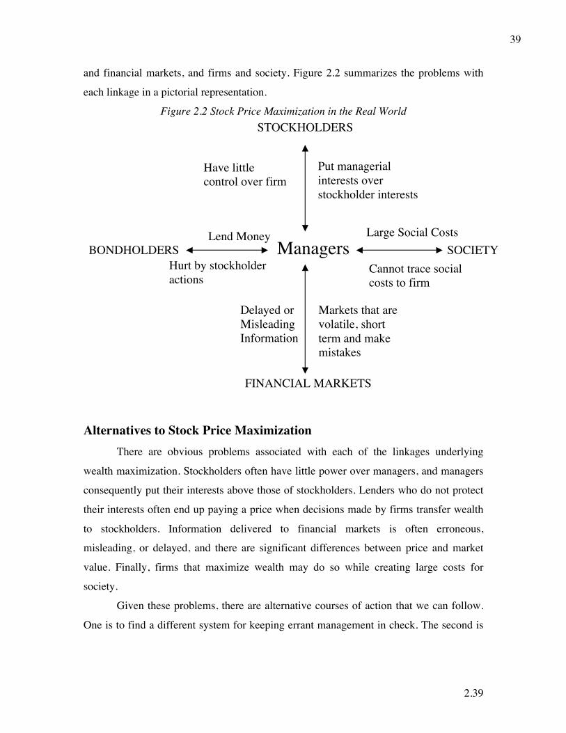
2.39

39

and financial markets, and firms and society. Figure 2.2 summarizes the problems with

each linkage in a pictorial representation.

Figure 2.2 Stock Price Maximization in the Real World STOCKHOLDERS

Put managerialinterests overstockholder interests

Have littlecontrol over firm

BONDHOLDERSLend Money

Hurt by stockholderactions

FINANCIAL MARKETS

SOCIETYManagers

Delayed orMisleadingInformation

Markets that arevolatile, shortterm and makemistakes

Large Social Costs

Cannot trace socialcosts to firm

Alternatives to Stock Price Maximization There are obvious problems associated with each of the linkages underlying

wealth maximization. Stockholders often have little power over managers, and managers

consequently put their interests above those of stockholders. Lenders who do not protect

their interests often end up paying a price when decisions made by firms transfer wealth

to stockholders. Information delivered to financial markets is often erroneous,

misleading, or delayed, and there are significant differences between price and market

value. Finally, firms that maximize wealth may do so while creating large costs for

society.

Given these problems, there are alternative courses of action that we can follow.

One is to find a different system for keeping errant management in check. The second is

2.40

40

to find an alternative objective for the firm. In this section, we will consider these

alternatives.

A Different System for Disciplining Management (Corporate Governance)

In the system we have described thus far, stockholders bear the burden of

replacing incompetent management; we can call this a market-based corporate

governance system, where investors in financial markets govern how corporations are

run. There are some who believe that this is too much of a responsibility to put on

investors, who, as they see it, often operate with poor information and have short time

horizons. Michael Porter, a leading thinker on corporate strategy, has argued that firms in

the United States are hamstrung by the fact that investors are short-term and demand

quick returns. He contrasts them with Japanese firms, which he argues can afford to adopt

strategies that make sense in the long run, even though they might not maximize profits

in the short term. He suggests that investors should form long-term relationships with

firms and work with them to devise long-term strategies.31 His view of the world is not

unique and is shared by many corporate executives, even in the United States. These

executives argue that there are alternatives to the market-based corporate governance

systems, where stockholders act to discipline and replace errant managers and stock

prices measure their success. In the German and Japanese systems of corporate

governance,32 firms own stakes in other firms and often make decisions in the best

interests of the industrial group they belong to rather than in their own interests. In these

systems, the argument goes, firms will keep an eye on each other, rather than ceding

power to the stockholders. In addition to being undemocratic—the stockholders are, after

all, the owners of the firm—these systems suggests a profound suspicion of how

stockholders might use the power if they get it and is heavily skewed toward maintaining

the power of incumbent managers.

31There is some movement toward relationship investing in the United States, where funds such as Allied Partners (run by Dillon Read), Corporate Partners (run by Lazard Freres), and Lens (run by activist Robert Monks) have attempted to create long-term relationships with the managers of firms. 32There are subtle differences between the Japanese and the German systems. The Japanese industrial groups, called keiretsus, are based primarily on cross-holdings of companies and evolved from family-owned businesses. The German industrial groups revolve around leading commercial banks, like Deutsche Bank or Dresdner Bank, with the bank holding substantial stakes in a number of industrial concerns.

2.41

41

Although this approach may protect the system against the waste that is a by-product

of stockholder activism and inefficient markets, it has its own disadvantages. Industrial

groups are inherently more conservative than investors in allocating resources and thus

are much less likely to finance high-risk and venture capital investments by upstarts who

do not belong to the group. The other problem is that entire groups can be dragged down

by the bad decisions of individual firms.33 In fact, the troubles that Japanese firms have

had dealing with poor investments in the 1990s suggests to us that these alternative

corporate governance systems, though efficient at dealing with individual firms that are

poorly run, have a more difficult time adapting to and dealing with problems that are

widespread. These problems, consequently, tend to fester and grow over time. For

instance, while financial markets pushed corporate banks in the United States to confront

their poor real estate loans in the late 1980s, Japanese banks spent much of the 1990s

denying the existence of such loans on their books.34

In the wake of the success of Chinese companies in the last decade and the

meltdown of global financial markets, there is another alternative being offered by those

who dislike the market-based mechanism. Why not let the government be a larger player

and decide where investments make the most sense? In the aftermath of a market

meltdown in 2008, with subsequent government bailouts of banks and troubled

companies, the number of advocates for an activist government role has increased even in

the United Kingdom and United States, historically countries that have been friendly to

market-based solutions. We remain skeptical for two reasons. The first is that history

does not provide much encouragement for government-driven investment. When

governments have tried to pick winners among companies, they have generally been

unsuccessful. Not only did the Soviet and other socialist based systems fail badly for

decades after the Second World War at planning economic growth, but enlightened

systems like the Japanese Ministry of Finance have not been able to forecast where

33Many Korean industrial groups (called chaebols), which were patterned after the Japanese keiretsu, were pushed to the verge of bankruptcy in 1990s because one or two errant firms in the group made bad real estate loans or borrowed too much. 34Kaplan, S. N., 1997, “Corporate Governance and Corporate Performance, A Comparison of German, Japan and the United States,” Journal of Applied Corporate Finance, 9(4), 86–93. He compares the U.S., German, and Japanese corporate governance systems. He finds that the U.S. system provides better incentives for firms performing well and that it is easier for companies in the United States to return cash to the stockholders.

2.42

42

growth will come from. The second is that governments have other agendas, besides

economic growth, and there can be conflicts between these different interests. Thus, even

if it is the best long-term economic interests of taxpayers in the United States to let GM

go under, it is unlikely that any government that has to face voters in Michigan (GM’s

home state) will be willing to let it happen. Finally, if the argument is that financial

markets are hotbeds of investor irrationality, note that government agencies are also

staffed with human beings, and there is no reason to believe that these decision makers

will be immune from making the same mistakes.

Is there a way we can measure the effectiveness of alternative corporate

governance systems? One suggestion is that corporate governance systems be measured

on three dimensions—the capacity to restrict management’s ability to obtain private

benefits from control, easy access to financial markets for firms that want capital, and the

ease with which inefficient management is replaced. It can be argued that a market-based

corporate governance system does a better job than alternative systems on all three

counts.35

Choosing an Alternative Objective

Given its limitations, the easy answer would be to cast aside stock price

maximization as an objective. The tough part is replacing it with another objective. It is

not that there are no alternatives, but that the alternatives come with their own sets of

problems and it is not at all obvious that there is a benefit to switching. This is especially

true when the alternative objective is evaluated on the three criteria used to evaluate the

wealth maximization objective: Is the objective clear and unambiguous? Does it come

with a timely measure that can be used to evaluate success and failure? Does it create side

costs that exceed the overall benefits? Let us consider three commonly offered

alternatives to stock price maximization.

I. Maximize Market Share

In the 1980s, Japanese firms inundated global markets with their products and

focused their attention on increasing market share. Their apparent success at converting

35Macey, J. R., 1998, “Measuring the Effectiveness of Different Corporate Governance Systems: Towards a More Scientific Approach,” Journal of Applied Corporate Finance, 10(4), 16–25.

2.43

43

this market share to profits led other firms, including some in the United States, to also

target market share as an objective. In concrete terms, this meant that investments that

increased market share more were viewed more favorably than investments that increased

them less. Proponents of this objective note that market share is observable and

measurable like market price and does not require any of the assumptions about efficient

financial markets that are needed to justify the stock price maximization objective.

Underlying the market share maximization objective is the belief (often unstated)

that higher market share will mean more pricing power and higher profits in the long run.

If this is in fact true, maximizing market share is entirely consistent with the objective of

maximizing firm value. However, if higher market share does not yield higher pricing

power, and the increase in market share is accompanied by lower or even negative

earnings, firms that concentrate on increasing market share can be worse off as a

consequence. In fact, many of the same Japanese firms that were used by corporate

strategists as their examples for why the focus on market share was a good one

discovered the harsh downside of this focus in the 1990s.

II. Profit Maximization Objectives

There are objectives that focus on profitability rather than value. The rationale for

them is that profits can be measured more easily than value, and that higher profits

translate into higher value in the long run. There are at least two problems with these

objectives. First, the emphasis on current profitability may result in short-term decisions

that maximize profits now at the expense of long-term profits and value. Second, the

notion that profits can be measured more precisely than value may be incorrect, given the

leeway that accountants have to shift profits across periods.

In its more sophisticated forms, profit maximization is restated in terms of

accounting returns (such as return on equity or capital) rather than dollar profits or even

as excess returns (over a cost of capital). Although these variants may remove some of

the problems associated with focusing on dollar profits next period, the problems with

accounting measurements carry over into them as well.

2.44

44

III. Size/Revenue Objectives

There are a whole set of objectives that have little to do with stockholder wealth

but focus instead on the size of the firm. In the 1970s, for instance, firms like Gulf &

Western and ITT, with strong CEOs at their helm, were built up through acquisitions into

giant conglomerates. There seemed to be no strategic imperative to these acquisitions,

other than the desire on the part of the CEOs to increase the sizes of their corporate

empires. Empire building may no longer be in vogue, but there have been cases where

corporations have made decisions that increase their size and perceived power at the

expense of stockholder wealth and profitability.

Maximize Stock Prices: Salvaging a Flawed Objective The alternatives to stock price maximization—a corporate governance system

build around self-governance or choosing a different objective like maximizing market

share—have their own limitations. In this section, we consider the case for salvaging

value maximization as an objective but consider ways we can reduce some of the

problems highlighted in the earlier section. In particular, we consider ways we can reduce

the conflicts of interest between stockholders, bondholders, and managers and the

potential for market failures. We also present an argument for market-based mechanisms

based on the market’s capacity to correct systematic mistakes quickly and effectively.

Conflict Resolution: Reducing Agency Problems

If the conflicts between stockholders, managers, and bondholders lie at the heart

of the problems with stock price maximization, reducing these conflicts should make it a

more palatable objective. In this section, we examine the linkages between stockholders

and managers, stockholders, and bondholders; firms and financial markets; and firms and

society and look at how best we can reduce the side costs to maximizing stock prices.

Stockholders and Managers

There are clearly conflicts of interests between stockholders and managers, and

the traditional mechanisms for stockholder control—annual meetings and boards of

directors—often fail at their role of discipline management. This does not mean,

however, that the chasm between the two groups is too wide to be bridged, either by

2.45

45

closing the gap between their interests or by increasing stockholder power over

managers.

Making Managers Think More Like Stockholders

As long as managers have interests that are distinct and different from the

interests of the stockholders they serve, there is potential for conflict. One way to reduce

this conflict is to provide managers with an equity stake in the firms they manage, either

by providing them with stock or warrants on the stock. If this is done, the benefits that

accrue to management from higher stock prices may provide an inducement to maximize

stock prices.

There is a downside to doing this, which is that although it reduces the conflict of

interest between stockholders and managers, it may exacerbate the other conflicts of

interest highlighted in the prior section. It may increase the potential for expropriation of

wealth from bondholders and the probability that misleading information will be

conveyed to financial markets.

There is a final distinction that we need

to make between stock-based compensation and

option-based compensation. As we will see in

the coming chapters, options can sometimes

become more valuable as businesses become

more risky. Consequently, managers who have substantial option holdings and little in

common stock may be tempted to take on far more risk than would be desired by other

shareholders in the firm. It is for this reason that companies are increasingly turning away

from option-based packages to restricted stock in compensating managers.

2.7. Stockholder Interests, Managerial Interests, and Management Buyouts In a management buyout, the managers of the firm buy out the existing stockholders and

make the company a private firm. Is this a way of reducing the conflict of interests

between stockholders and managers? Explain.

Yes

No

Warrants: A warrant is a security issued by a

company that provides the holder with the

right to buy a share of stock in the company

at a fixed price during the life of the warrant.

2.46

46

More Effective Boards of Directors

In the past few years, there have been encouraging trends both in the composition

and the behavior of boards, making them more effective advocates for stockholders.

Korn/Ferry’s survey of boards of directors at large global corporations in 2007 revealed

the following.

• Boards have become smaller over time. The median size of a board of directors has

decreased from a range of between sixteen and twenty in the 1970s to ten in 2007.

The smaller boards are less unwieldy and more effective than larger boards.

• There are fewer insiders on the board. In contrast to the six or more insiders that

many boards had in the 1970s, only two directors in most boards in 2007 were

insiders.

• Directors are increasingly compensated with equity in the company. In 1973, only 4

percent of directors received compensation in the form of equity, whereas 86 percent

did so in 2007. There has also been a shift away from options to restricted stock; 72%

of firms used restricted stock and only 14% used options. While the use of restricted

stock in compensation has increased in Europe as well, it is still uncommon in Asia.

• More directors are identified and selected by a nominating committee rather than

being chosen by the CEO of the firm. In 2007, 97 percent of boards had nominating

committees; the comparable statistic in 1973 was 2 percent.

• More firms restrict the number of outside directorships held by their directors: In

2001, only 23% of firms limited the number of other board memberships of their

directors. In 2007, that number had risen to 62%. While many UK and European

companies also restrict board memberships, such restrictions are less common in

Asia.

• More firms have appointed lead directors to counter the CEO as chair: While it was

unusual for boards to appoint lead directors 20 years ago, almost 84% of US boards

now have a lead director to serve as a counterweight to the CEO.

• More firms are evaluating CEOs on an annual basis: in 1999, 56% of US corporate

boards evaluated CEOs on an annual basis. That number had risen to 92% in 2007. In

Asia, almost 95% of boards claim to evaluate CEOs on an annual basis.

2.47

47

While these are all positive trends, there are two precautionary notes that we add. The

first is that the survey focused on large companies and board practices at smaller

companies have been much slower to change. The second is that it is not clear how much

of this change is window dressing, giving the appearance of active oversight to prevent

lawsuits.

Is there a payoff to a more active board? MacAvoy and Millstein (1998) present

evidence that companies with more activist boards, where activism was measured based

upon indicators of board behavior, earned much higher returns on their capital than firms

that had less active boards.36 As hedge funds and activist investors have raised their

profile in the last few years, there is evidence that directors that they place on the boards

of challenged companies make a difference, at least in stock price performance. A study

by the Investor Responsibility Research Center (IRRC) of 120 companies with hybrid

boards, i.e., boards with directors elected by activist investors, found that their stock

prices outperformed their peer group by almost 17% a year, with the bulk of the return

occurring around the months that activists challenged the company. Interestingly, the

performance of companies with a single dissident director elected was much better than

those where three or more dissident directors were elected.

Increasing Stockholder Power

There are many ways in which stockholder power over management can be

increased. The first is to provide stockholders with better and more updated information,

so that they can make informed judgments on how well the management is doing. The

second is to have a large stockholder become part of incumbent management and have a

direct role in decisions that the firm makes. The third is to have more “activist”

institutional stockholders, who play a larger role in issues such as the composition of the

board of directors, the question of whether to pass antitakeover amendments, and overall

management policy. In recent years, some institutional investors have used their

considerable power to pressure managers into becoming more responsive to their needs.

Among the most aggressive of these investors has been the California State Pension fund

(CALPERS), one of the largest institutional investors in the country. Unfortunately, the

2.48

48

largest institutional investors—mutual funds and pension fund companies—have

remained largely apathetic. In the last few years, hedge funds have stepped into the

breach and have challenged even large companies to defend existing practices.

It is also critical that institutional constraints on stockholders exercising their

power be reduced. All common shares should have the same voting rights, state

restrictions on takeovers have to be eliminated and shareholder voting should be

simplified. The legal system should come down hard on managers (and boards of

directors) who fail to do their fiduciary duty. Ultimately, though, stockholders have to

awaken to the reality that the responsibility for monitoring management falls to them.

Like voters in a democracy, shareholders get the managers they deserve.

In Practice: The Legal Remedy

Can we legislate good corporate governance? Whether we can or not, legislators

often try to fix what they see as significant corporate governance problems by passing

laws. This is especially true in the aftermath of scandals, where stockholders,

bondholders and society bear the cost of managerial incompetence. As an example, after

the accounting scandals in the United States in 2001 and 2002, the Sarbanes-Oxley Act

was passed with the explicit intent of preventing future Enrons and Worldcoms. The act

was far reaching in its coverage but large parts of it related to the composition of

corporate boards and the responsibilities of boards. Without going into the provisions of

the law, the objective was to create more transparency in the way boards were created,

increase the independence of the directors from the CEO and the legal responsibilities of

directors for managerial actions. Sarbanes Oxley also substantially increased the

information disclosure requirements for firms.

The other legal remedy that stockholders have is to sue the managers when they

feel that they have been misled about future prospects. In recent years, class action

lawsuits against companies whose stock prices have plummeted have multiplied and the

plaintiffs have won large awards in some of these suits. While the right to sue when

wronged may seem fundamental, legal remedies are likely to be both imperfect and very

expensive ways of bringing about better corporate governance. In fact, the cost of

36 See MacAvoy, P.W. and I.M. Millstein, 1998, The Active Board of Directors and its Effect on the Performance of Large Publicly Traded Companies, Columbia Law Review, v98, 1283-1322.

2.49

49

complying with Sarbanes Oxley has been substantial and the only group that consistently

is enriched by lawsuits is trial lawyers.

2.8. Inside Stockholders versus Outside Stockholders There are companies like Microsoft where a large stockholder (Bill Gates) may be the on

the inside as the top manager of the concern. Is it possible that what is in Bill Gates’s best

interests as an “inside” stockholder may not be in the interests of a stockholder on the

outside?

Yes. Their interests may deviate.

No. Their interests will not deviate.

If yes, provide an example of an action that may benefit the inside stockholder but not the

outside stockholder.

The Threat of a Takeover

The perceived excesses of many takeovers in the 1980s drew attention to the

damage created to employees and society some of them. In movies and books, the raiders

who were involved in these takeovers were portrayed as barbarians, while the firms being

taken over were viewed as hapless victims. Although this may have been accurate in

some cases, the reality was that most companies that were taken over deserved it. One

analysis found that target firms in hostile takeovers in 1985 and 1986 were generally

much less profitable than their competitors, had provided subpar returns to their

stockholders, and had managers with significantly lower holdings of the equity. In short,

badly managed firms were much more likely to become targets of hostile takeover bids.37

An implication of this finding is that takeovers operate as a disciplinary

mechanism, keeping managers in check, by introducing a cost to bad management. Often,

the very threat of a takeover is sufficient to make firms restructure their assets and

become more responsive to stockholder concerns. It is not surprising, therefore, that legal

attempts to regulate and restrict takeovers have had negative consequences for stock

prices.

37Bhide, A., 1989, “The Causes and Consequences of Hostile Takeovers,” Journal of Applied Corporate Finance, 2, 36–59.

2.50

50

2.9. Hostile Acquisitions: Whom Do They Hurt? Given the information presented in this chapter, which of the following groups is

likely to be the most likely to be protected by a law banning hostile takeovers?

Stockholders of target companies

Managers and employees of well-run target companies

Managers and employees of badly run target companies

Society

Illustration 2.5 Restive Stockholders and Responsive Managers: The Disney Case

In 1997, Disney was widely perceived as having an imperial CEO in Michael

Eisner and a captive board of directors. After a series of missteps including the hiring and

firing of Michael Ovitz and bloated pay packages, Disney stockholders were restive, but

there were no signs of an impending revolt at that time. As Disney’s stock price slid

between 1997 and 2000, though, this changed as more institutional investors made their

displeasure with the state of corporate governance at the company. As talk of hostile

takeovers and proxy fights filled the air, Disney was forced to respond. In its 2002 annual

report, Disney listed the following corporate governance changes:

• Required at least two executive sessions of the board, without the CEO or other

members of management present, each year.

• Created the position of management presiding director and appointed Senator

George Mitchell to lead those executive sessions and assist in setting the work

agenda of the board.

• Adopted a new and more rigorous definition of director independence.

• Required that a substantial majority of the board be made up of directors meeting

the new independence standards.

• Provided for a reduction in committee size and the rotation of committee and

chairmanship assignments among independent directors.

• Added new provisions for management succession planning and evaluations of

both management and board performance.

• Provided for enhanced continuing education and training for board members.

2.51

51

What changed between 1997 and 2002? Although we can point to an overall shift in the

market toward stronger corporate governance, the biggest factor was poor stock price

performance. The truth is that stockholders are often willing to overlook poor corporate

governance and dictatorial CEOs if stock prices are going up but are less tolerant when

stock prices decrease.

Toward the end of 2003, Roy Disney and Stanley Gold resigned from Disney’s

board of directors, complaining both about the failures of Eisner and about his autocratic

style.38 When the board of directors announced early in 2004 that Eisner would receive a

$6.25 million bonus for his performance in 2003, some institutional investors voiced their

opposition. Soon after, Comcast announced a hostile acquisition bid for Disney. At

Disney’s annual meeting in February 2004, Disney and Gold raised concerns about

Eisner’s management style and the still-captive board of directors; 43 percent of the

stockholders voted against Eisner as director at the meeting. In a sense, the stars were

lining up for the perfect corporate governance storm at Disney, with Eisner in the eye of

the storm. Soon after the meeting, Disney announced that Eisner would step down as

chairman of the board even though he would continue as CEO until his term expired in

2005.

In Practice Proxy Fights

In the section on annual meetings, we pointed out that many investors who are

unable to come to annual meetings also fail to return their proxies, thus implicitly giving

incumbent managers their votes. In a proxy fight, activist investors who want to

challenge incumbent managers approach individual stockholders in the company and

solicit their proxies, which they then can use in votes against the management slate.

In one very public and expensive proxy fight in 2002, David Hewlett, who was

sitting on the board of Hewlett Packard (HP) at the time, tried to stop HP from buying

Compaq by soliciting proxies from HP stockholders. After eight months of acrimony, HP

finally won the fight with the bare minimum 51 percent of the votes. How did David

Hewlett come so close to stopping the deal? One advantage he had was that the Hewlett

and Packard families owned a combined 18 percent of the total number of shares

outstanding. The other was that Hewlett’s position on the board and his access to internal

2.52

52

information gave him a great deal of credibility when it came to fighting for the votes of

institutional investors. The fact that he failed, even with these advantages, shows how

difficult it is to win at a proxy fight. Even a failed proxy fight, though, often has the

salutary effect of awakening incumbent managers to the need to at least consider what

shareholders want.

Stockholders and Bondholders

The conflict of interests between stockholders and bondholders can lead to actions

that transfer wealth to the former from the latter. There are ways bondholders can obtain

at least partial protection against some of these actions.

The Effect of Covenants

The most direct way for bondholders to protect themselves is to write in

covenants in their bond agreements specifically prohibiting or restricting actions that may

make them worse off. Many bond (and bank loan) agreements have covenants that do the

following.

1. Restrict the firm’s investment policy. Investing in riskier businesses than

anticipated can lead to a transfer of wealth from bondholders to stockholders.

Some bond agreements put restrictions on where firms can invest and how much

risk they can take on in their new investments, specifically to provide bondholders

with the power to veto actions that are not in their best interests.

2. Restrict dividend policy. In general, increases in dividends increase stock prices

while decreasing bond prices because they reduce the cash available to the firm to

meet debt payments. Many bond agreements restrict dividend policy by tying

dividend payments to earnings.

3. Restrict additional leverage. Some bond agreements require firms to get the

consent of existing lenders before borrowing more money. This is done to protect

the interests of existing secured bondholders.

Although covenants can be effective at protecting bondholders against some abuses, they

do come with a price tag. In particular, firms may find themselves having to turn down

profitable investments because of bondholder-imposed constraints and having to pay

38You can read Roy Disney’s letter of resignation on the Web site for the book.

2.53

53

(indirectly through higher interest rates) for the legal and monitoring costs associated

with the constraints.

Taking an Equity Stake

Because the primary reason for the conflict of interests between stockholders and

bondholders lies in the nature of their claims, another way that bondholders can reduce

the conflict of interest is by owning an equity stake in the firm. This can take the form of

buying equity in the firm at the same time as they lend money to it, or it can be

accomplished by making bonds convertible into stock at the option of the bondholders. In

either case, bondholders who feel that equity investors are enriching themselves at the

lenders’ expense can become stockholders and share in the spoils.

Bond Innovations

In the aftermath of several bond market debacles in the late 1980s, bondholders

became increasingly creative in protecting themselves with new types of bonds. Although

we will consider these innovations in more detail later in this book, consider the example

of puttable bonds. Unlike a conventional bond, where you are constrained to hold the

bond to maturity, the holders of a puttable bond can put the bond back to the issuing

company and get the face value of the bond if the company violates the conditions of the

bond. For instance, a sudden increase in borrowing by the company or a drop in its bond

rating can trigger this action.

In Practice: Hedge Funds and Corporate Governance

In the last few years, hedge funds have become key players in the corporate governance

battle. They have accumulated large shares in many companies, including some large

market cap firms, and then used those shares to nominate directors and challenge

management. While this may seem like an unmitigated good, at least from the

perspective of corporate governance, there are four reasons that for concern:

a. Management shakedowns: There have been cases where hedge funds have banded

together, threatened management with dire consequences and used that threat to

extract side payments and special deals for themselves. In the process, other

stockholders are made worse off.

2.54

54

b. Short term objectives: Some hedge funds have short term objectives that may diverge

from the long term interests of the firm. Giving hedge funds more of a say in how

companies are run can lead to decisions that feed into these short term interests, while

damaging long term firm value.

c. Competing interests: Since hedge funds can go long or short and invest in different

markets (bonds and derivatives), it is conceivable for a hedge fund that owns equity

in firm to also have other positions in the firm that may benefit when the value of

equity drops. For instance, a hedge fund that owns stock in a company and has bet on

the firm’s demise in the derivatives market may use its voting power to drive the

company into bankruptcy.

d. Herd Mentality: While we assume that hedge fund managers are somehow smarter

and more sophisticated than the rest of the market, they are not immune from the

behavioral characteristics that bedevil other investors. In fact, the herd mentality

seems to drive many hedge funds, who flock to the same companies at the same time

and their prescriptions for corporate renewal seem to follow the same script.

In spite of these concerns, we believe that the presence of hedge funds and activist

investors in the mix of stockholders empowers other stockholders, for the most part, not

because the changes they suggest are always wise or that management is always wrong

but because they force managers to explain their actions (on capital structure, asset

deployment and dividends) to stockholders.

Firms and Financial Markets

The information that firms convey to financial markets is often erroneous and

sometimes misleading. The market price that emerges from financial markets can be

wrong, partly because of inefficiencies in markets and partly because of the errors in the

information. There are no easy or quick fix solutions to these problems. In the long run,

however, there are actions that will improve information quality and reduce deviations

between price and value.

Improving the Quality of Information

Although regulatory bodies like the SEC can require firms to reveal more

information and penalize those that provide misleading and fraudulent information, the

2.55

55

quality of information cannot be improved with information disclosure laws alone. In

particular, firms will always have a vested interest in when and what information they

reveal to markets. To provide balance, therefore, an active external market for

information has to exist where analysts who are not hired and fired by the firms that they

follow collect and disseminate information. These analysts are just as likely to make

mistakes as the firm, but they presumably should have a greater incentive to unearth bad

news about the firm and disseminate that information to their clients. For this system to

work, analysts have to be given free rein to search for good as well as bad news and make

positive or negative judgments about a firm.

Making Markets More Efficient

Just as better information cannot be legislated into existence, markets cannot be

made more efficient by edict. In fact, there is widespread disagreement on what is

required to make markets more efficient. At the minimum, these are necessary (though

not sufficient) conditions for more efficient markets:

• Trading should be both inexpensive and easy. The higher transactions costs are,

and the more difficult it is to execute a trade, the more likely it is that markets will

be inefficient.

• There should be free and wide access to information about firms.

• Investors should be allowed to benefit when they pick the right stocks to invest in

and to pay the price when they make mistakes.

Restrictions imposed on trading, although well intentioned, often lead to market

inefficiencies. For instance, restricting short sales, where investors who don’t own a stock

can borrow and sell it if they feel it is overpriced, may seem like good public policy, but

it can create a scenario in which negative information about stocks cannot be reflected

adequately in prices.

Short term versus Long term

Even in liquid markets with significant information about companies, investors

not only make mistakes, but make these mistakes systematically for extended periods, for

the behavioral reasons that we noted earlier. In other words, there is no way to ensure that

stock prices will not deviate from value for extended periods. As a consequence, even

2.56

56

believers in stock price maximization need to pause and consider the possibility that

doing what is right for a company’s long-term value may result, at least in the short term,

in lower stock prices. Conversely, actions that hurt the long-term interests of the firm

may be accompanied by higher stock prices.

The lesson for corporate governance is a simple one. Managers should not be

judged and compensated based upon stock price performance over short periods. If

compensation is tied to stock prices, a portion of the compensation has to be held back to

ensure that management actions are in the best long-term interests of the company. More

companies now have claw-back provisions in compensation contracts, allowing them to

reclaim compensation from earlier years in case stock prices come down after the initial

blip, or require managers to wait to cash out their compensation. With restricted stock,

for instance, managers often have to wait three or five years before the stock can be

liquidated. Implicitly, we are assuming that stock prices ultimately will reflect the true

value.

Firms and Society

There will always be social costs associated with actions taken by firms, operating

in their own best interests. The basic conundrum is as follows: Social costs cannot be

ignored in making decisions, but they are also too nebulous to be factored explicitly into

analyses. One solution is for firms to maximize firm or stockholder value, subject to a

good citizen constraint, where attempts are made to minimize or alleviate social costs,

even though the firm may not be under any legal obligation to do so. The problem with

this approach, of course, is that the definition of a good citizen is likely to vary from firm

to firm and from manager to manager.

Ultimately, the most effective way to make companies more socially responsible

is to make it in their best economic interests to behave well. This can occur in two ways.

First, firms that are construed as socially irresponsible could lose customers and profits.

This was the galvanizing factor behind a number of specialty retailers in the United States

disavowing the use of sweatshops and underage labor in other countries in making their

products. Second, investors might avoid buying stock in these companies. As an example,

many U.S. college and state pension plans have started reducing or eliminating their

2.57

57

holding of tobacco stocks to reflect their concerns about the health effects of tobacco. In

fact, investors now have access to “ethical mutual funds,” which invest only in

companies that meet a social consciousness threshold. Figure 2.3 summarizes the ways in

which we can reduce potential side costs from stock price maximization.

Figure 2.3 here STOCKHOLDERS

Managers think likestockholders

1. Stock-basedcompensation2. Hostile takeovers3. Activist investors

BONDHOLDERSLend Money

Protect themselves withcovenants and new bondstypes

FINANCIAL MARKETS

SOCIETYManagers

More externalinformation-Active analysts

More liquid marketswith lowertransactions costs

Reduced Social Costs

1. Laws and Restrictions2. Investor/ Customer Backlash

In Practice Can You Add Value while Doing Good?

Does doing social good hurt or help firms? On one side of this argument stand

those who believe that firms that expend considerable resources to generate social good

are misguided and are doing their stockholders a disservice. On the other side are those

who believe that socially conscious firms are rewarded by consumers (with higher sales)

and by investors (with higher values). The evidence is mixed and will undoubtedly

disappoint both sides.

• Studies indicate that the returns earned by stockholders in socially conscious

firms are no different than the returns earned by stockholders in the rest of the

market. Studies of ethical mutual funds find that they neither lag nor lead other

mutual funds.

2.58

58

• There is clearly a substantial economic cost borne by companies that are viewed

by society as beyond the pale when it comes to creating social costs. Tobacco

firms, for instance, have seen stock prices slide as investors avoid their shares and

profits hurt by legal costs.

• When firms are profitable and doing well, stockholders are usually willing to give

managers the flexibility to use company money to do social good. Few investors

in Microsoft begrudged its 1998 decision to give free computers to public libraries

around the country. In firms that are doing badly, stockholders tend to be much

more resistant to spending company money in mending society’s ills.

Summarizing this evidence, we can draw some conclusions. First, a firm’s foremost

obligation is to stay financially healthy and increase value; firms that are losing money

cannot afford to be charitable. Second, firms that create large social costs pay a high price

in the long run. Finally, managers should not keep stockholders in the dark about the cost

of meeting social obligations; after all, it is the stockholders’ money that is being used for

the purpose.

A Compromise Solution: Value Maximization with Price Feedback Let us start off by conceding that all of the alternatives—choosing a different

corporate governance system, picking an alternative objective and maximizing stock

price with constraints—have limitations and lead to problems. The questions then

become how each alternative deals with mistakes and how quickly errors get corrected.

This is where a market-based system does better than the alternatives. It is the only one of

the three that is self-correcting, in the sense that excesses by any stakeholder attract

responses in three waves.

1. Market reaction. The first and most immediate reaction comes from financial markets.

Consider again the turmoil created when we have well-publicized failures like Enron. Not

only did the market punish Enron (by knocking its stock and bond prices down) but it

punished other companies that it perceived as being exposed to the same problems as

Enron—weak corporate governance and opaque financial statements—by discounting

their values as well.

2.59

59

2. Group activism. Following on the heels of the market reaction to any excess is outrage

on the part of those who feel that they have been victimized by it. In response to

management excesses in the 1980s, we saw an increase in the number of activist

investors and hostile acquisitions, reminding managers that there are limits to their

power. In the aftermath of well-publicized scandals in the late 1980s where loopholes in

lending agreements were exploited by firms, banks and bondholders began playing more

active roles in management.

3. Market innovations. Markets often come up with innovative solutions to problems. In

response to the corporate governance scandals in 2002 and 2003, Institutional

Shareholder Services began scoring corporate boards on independence and effectiveness

and offering these scores to investors. After the accounting scandals of the same period,

the demand for forensic accounting, where accountants go over financial statements

looking for clues of accounting malfeasance, increased dramatically. The bond market

debacles of the 1980s gave birth to dozens of innovative bonds designed to protect

bondholders. Even in the area of social costs, there are markets that have developed to

quantify the cost.

Having made this argument for market-based mechanisms, we also need to be

realistic. To the extent that market prices and value can deviate, tying corporate financial

decisions to current stock prices can sometimes lead to bad decisions. As a blueprint for

decision-making, here is what we would suggest:

1. Focus on long term value: Managers should make decisions that maximize the

long-term value of the firm. This will of course require that we be more explicit

about the link between operating and financial decisions and value and we will do

so in the coming chapters.

2. Improve corporate governance: Having an independent and informed board of

directors can help top managers by providing feedback on major decisions and by

acting as a check on management ambitions. The quality of this feedback will

improve if there are adversarial directors on the board. In fact, having an

independent director take the role of devil’s advocate may force managers to think

through the consequences of their decisions.

2.60

60

3. Increase transparency: When managers make decisions that they believe are in the

best long-term interests of the firm, they should make every attempt to be

transparent with financial markets about the motivation for and the consequences

of these decisions. Too often, managers hold back critical information from

markets or engage in obfuscation when dealing with markets.

4. Listen to the market: If the market reaction is not consistent with management

expectations, i.e., the stock price goes down when markets receive news about a

what managers believe to be a value-increasing decision, managers should

consider the message in the market reaction. There are three possible

explanations.

• The first is that the information provided about the decision is incomplete and

or not convincing, in which case framing the decision better for betters may be

all that is required. (Public relations response)

• The second is that investors are being swayed by irrational factors and are

responding in accordance. In this case, managers should consider modifying

the decision to make it palatable to investors, as long as these modifications

do not alter the value enhancement dynamic.

• The third is that the market is right in its assessment that the decision will

destroy and not increase value. In this case, managers should be willing to

abandon decisions. While markets are not always right, they should never be

ignored and managers should consider modifying their decisions to reflect the

market reaction.

5. Tie rewards to long-term value: Any management compensation and reward

mechanisms in the firm should be tied to long-term value. Since market prices

remain the only tangible manifestation of this value, this implies that any equity

compensation (options or restricted stock) be tied to the long-term stock price

performance of a firm and not the short term.

Since this mechanism is central to how we will frame key corporate finance decisions,

figure 2.4 summarizes the process with the feedback loops:

2.61

61

Figure 2.4: Value Maximization with Feedback

Maximize long term valueWhen making decisions, focus on increaasing the long term value of the firm.

Get board inputDescribe decisions and motivation to the board of directors.

Information to marketDescribe decision and explain why it will increase long term value

Favorable feedback

Watch market reactionLook at the response of the market to information about decision

Market price increases

Negative feedbackRevisit, modify and abandon decision

Market price decreases. Examine why. and perhaps reframe (if poor information), modify or abandon decision.

Tie rewards to long term valueCompensation should be tied to stock price performance in the long term and not the short term

To improve process

Managers should not only understand business but also the link between decisions and value

Directors should be independent, involved and informed. Having a lead director play devilʼs advocate may be a good idea..

Be transparent and provide full information. There should be less selling (fewer buzzwords) and more explanation (analysis).

More liquid markets with diverse traders will generate more informative prices.

Hold back portions of compensation until you get confirmation of long term value increase.

Decision Process Feedback

A confession is in order here. In earlier editions of this book, we argued that the objective

in corporate finance should be stock price maximization, notwithstanding the failures of

financial markets. This is the first time that we have strayed from this classical objective,

illustrating not only the effects of the market turmoil of 2008-2009 but also the collective

evidence that has accumulated that investors are not always rational in the way they price

assets, at least in the short term.

We will stay with this framework as we make our way through each major

corporate finance decision. With investment, financing and dividend policies, we will

begin by focusing on the link between policy and value and what we believe is the best

approach for maximizing value. We will follow up by examining what information about

these decisions has to be provided to financial markets and why markets may provide

dissonant feedback. Finally, we will consider how best to incorporate this market

2.62

62

feedback into decisions (and the information we provide about these decisions) to

increase the changes of aligning long term value and stock prices.

A Postscript: The Limits of Corporate Finance Corporate finance has come in for more than its fair share of criticism in the past

decade or so. There are many who argue that the failures of corporate America can be

traced to its dependence on financial markets. Some of the criticism is justified and based

on the limitations of a single-minded pursuit of stock price maximization. Some of it,

however, is based on a misunderstanding of what corporate finance is about.

Economics was once branded the gospel of Mammon, because of its emphasis on

wealth. The descendants of those critics have labeled corporate finance as unethical,

because of its emphasis on the bottom line and market prices. In restructuring and

liquidations, it is true that value maximization for stockholders may mean that other

stakeholders, such as customers and employees, lose out. In most cases, however,

decisions that increase market value also make customers and employees better off.

Furthermore, if the firm is really in trouble, either because it is being undersold by

competitors or because its products are technologically obsolete, the choice is not

between liquidation and survival but between a speedy resolution, which is what

corporate financial theory would recommend, and a slow death, while the firm declines

over time and costs society considerably more in the process.

The conflict between wealth maximization for the firm and social welfare is the

genesis for the attention paid to ethics in business schools. There will never be an

objective set of decision rules that perfectly factor in societal concerns, simply because

many of these concerns are difficult to quantify and are subjective. Thus, corporate

financial theory, in some sense, assumes that decision makers will not make decisions

that create large social costs. This assumption that decision makers are for the most part

ethical and will not create unreasonable costs for society or for other stakeholders is

unstated but underlies corporate financial theory. When it is violated, it exposes corporate

financial theory to ethical and moral criticism, though the criticism may be better directed

at the violators.

2.63

63

2.10. What Do You Think the Objective of the Firm Should Be? Having heard the pros and cons of the different objectives, the following statement best

describes where I stand in terms of the right objective for decision making in a business.

Maximize stock price or stockholder wealth, with no constraints

Maximize stock price or stockholder wealth, with constraints on being a good social

citizen

Maximize profits or profitability

Maximize market share

Maximize revenues

Maximize social good

None of the above

Conclusion Although the objective in corporate finance is to maximize firm value, in practice

we often adopt the narrower objective of maximizing a firm’s stock price. As a

measurable and unambiguous measure of a firm’s success, stock price offers a clear

target for managers in the course of their decision-making. Implicitly, we are assuming

that the stock price is a reasonable and unbiased estimate of the true value of the

company and that any action that increases stock prices also increases value.

Stock price maximization as the only objective can be problematic when the

different players in the firm—stockholders, managers, lenders, and society—all have

different interests and work at cross-purposes. These differences, which result in agency

costs, can result in managers who put their interests over those of the stockholders who

hired them, stockholders who try to take advantage of lenders, firms that try to mislead

financial markets, and decisions that create large costs for society. In the presence of

these agency problems, there are many who argue for an alternative to stock price

maximization. Although this path is alluring, each of the alternatives, including using a

different system of corporate governance or a different objective, comes with its own set

of limitations. Stock price maximization also fails when markets do not operate

efficiently and stock prices deviate from true value for extended periods, and there is

mounting evidence that they do.

2.64

64

Given the limitations of the alternatives, we will split the difference. We believe

that managers should make decisions that increase the long-term value of the firm and

then try to provide as much information as they can about the consequences of these

decisions to financial markets. If the market reaction is not positive, they should pay

attention, since there is a message in the price reaction that may lead them to modify their

decisions.

2.65

65

Live Case Study

I. Corporate Governance Analysis

Objective: To analyze the corporate governance structure of the firm and assess where

the power in the firm lies and the potential for conflicts of interest at the firm.

Key Questions

• Is this a company where there is a separation between management and ownership? If

so, how responsive is management to stockholders?

• Is there a potential conflict between stockholders and lenders to the firm? If so, how

is it managed?

• How does this firm interact with financial markets? How do markets get information

about the firm?

• How does this firm view its social obligations and manage its image in society?

Framework for Analysis

1. The Chief Executive Officer

• Who is the CEO of the company? How long has he or she been CEO?

• If it is a “family-run” company, is the CEO part of the family? If not, what

career path did the CEO take to get to the top? (Did he or she come from

within the organization or from outside?)

• How much did the CEO make last year? What form did the compensation take

(salary, bonus, and option components)?

• How much equity in the company does the CEO own and in what form

(stocks or options)?

2. The Board of Directors

• Who is on the board of directors of the company? How long have they served

as directors?

• How many of the directors are inside directors?

• How many of the directors have other connections to the firm (as suppliers,

clients, customers, etc.)?

• How many of the directors are CEOs of other companies?

• Do any of the directors have large stockholdings or represent those who do?

2.66

66

3. Bondholder Concerns

• Does the firm have any publicly traded debt?

• Are there are bond covenants (that you can uncover) that have been imposed

on the firm as part of the borrowing?

• Do any of the bonds issued by the firm come with special protections against

stockholder expropriation?

4. Financial Market Considerations

• How widely held and traded is the stock? What proportion of its shares are

widely traded (floats)?

• How many analysts follow the firm?

• How much trading volume is there on this stock?

5. Societal Constraints

• What does the firm say about its social responsibilities?

• Does the firm have a particularly good or bad reputation as a corporate

citizen?

• If it does, how has it earned this reputation?

• If the firm has been a recent target of social criticism, how has it responded?

Information Sources

For firms that are incorporated in the United States, information on the CEO and

the board of directors is primarily in the filings made by the firm with the SEC. In

particular, the 14-DEF will list the directors in the firm, their relationship with the firm,

and details on compensation for both directors and top managers. You can also get

information on trading done by insiders from the SEC filings. For firms that are not

listed in the United States, this information is much more difficult to obtain. However,

the absence of readily accessible information on directors and top management is more

revealing about the power that resides with incumbent managers.

Information on a firm’s relationships with bondholders usually resides in the

firm’s bond agreements and loan covenants. Although this information may not always

be available to the public, the presence of constraints shows up indirectly in the firm’s

bond ratings and when the firm issues new bonds.

2.67

67

The relationship between firms and financial markets is tougher to gauge. The list

of analysts following a firm can be obtained from publications, such as the Nelson

Directory of Securities Research. For larger and more heavily followed firms, the

archives of financial publications (the Financial Times, Wall Street Journal, Forbes,

Barron’s) can be useful sources of information.

Finally, the reputation of a firm as a corporate citizen is the most difficult area to

obtain clear information on, because it is only the outliers (the worst and the best

corporate citizens) that make the news. The proliferation of socially responsible mutual

funds, however, does give us a window on those firms that pass the tests (arbitrary

though they sometimes are) imposed by these funds for a firm to be viewed as socially

responsible.

Online sources of information: www.stern.nyu.edu/~adamodar/cfin2E/project/data.htm.

2.68

68

Problems and Questions

1. There is a conflict of interest between stockholders and managers. In theory,

stockholders are expected to exercise control over managers through the annual meeting

or the board of directors. In practice, why might these disciplinary mechanisms not work?

2. Stockholders can transfer wealth from bondholders through a variety of actions. How

would the following actions by stockholders transfer wealth from bondholders?

a. An increase in dividends

b. A leveraged buyout

c. Acquiring a risky business

How would bondholders protect themselves against these actions?

3. Stock prices are much too volatile for financial markets to be efficient. Comment.

4. Maximizing stock prices does not make sense because investors focus on short-term

results and not on the long-term consequences. Comment.

5. There are some corporate strategists who have suggested that firms focus on

maximizing market share rather than market prices. When might this strategy work, and

when might it fail?

6. Antitakeover amendments can be in the best interests of stockholders. Under what

conditions is this likely to be true?

7. Companies outside the United States often have two classes of stock outstanding. One

class of shares is voting and is held by the incumbent managers of the firm. The other

class is nonvoting and represents the bulk of traded shares. What are the consequences

for corporate governance?

8. In recent years, top managers have been given large packages of options, giving them

the right to buy stock in the firm at a fixed price. Will these compensation schemes make

managers more responsive to stockholders? Why or why not? Are lenders to the firm

affected by these compensation schemes?

2.69

69

9. Reader’s Digest has voting and nonvoting shares. About 70 percent of the voting

shares are held by charitable institutions, which are headed by the CEO of Reader’s

Digest. Assume that you are a large holder of the nonvoting shares. Would you be

concerned about this set-up? What are some of the actions you might push the firm to

take to protect your interests?

10. In Germany, large banks are often large lenders and large equity investors in the same

firm. For instance, Deutsche Bank is the largest stockholder in Daimler Chrysler, as well

as its largest lender. What are some of the potential conflicts that you see in these dual

holdings?

11. It is often argued that managers, when asked to maximize stock price, have to choose

between being socially responsible and carrying out their fiduciary duty. Do you agree?

Can you provide an example where social responsibility and firm value maximization go

hand in hand?

12. Assume that you are advising a Turkish firm on corporate financial questions, and

that you do not believe that the Turkish stock market is efficient. Would you recommend

stock price maximization as the objective? If not, what would you recommend?

13. It has been argued by some that convertible bonds (i.e., bonds that are convertible

into stock at the option of the bondholders) provide one form of protection against

expropriation by stockholders. On what is this argument based?

14. Societies attempt to keep private interests in line by legislating against behavior that

might create social costs (such as polluting the water). If the legislation is comprehensive

enough, does the problem of social costs cease to exist? Why or why not?

15. One of the arguments made for having legislation restricting hostile takeovers is that

unscrupulous speculators may take over well-run firms and destroy them for personal

gain. Allowing for the possibility that this could happen, do you think that this is

sensible? If so, why? If not, why not?

2.70

70

1

CHAPTER 3

THE BASICS OF RISK

Risk, in traditional terms, is viewed as a negative and something to be avoided.

Webster’s dictionary, for instance, defines risk as “exposing to danger or hazard”. The

Chinese symbols for risk, reproduced below, give a much better description of risk –

危机 The first symbol is the symbol for “danger”, while the second is the symbol for

“opportunity”, making risk a mix of danger and opportunity. It illustrates very clearly the

tradeoff that every investor and business has to make – between the “higher rewards” that

potentially come with the opportunity and the “higher risk” that has to be borne as a

consequence of the danger. The key test in finance is to ensure that when an investor is

exposed to risk that he or she is “appropriately” rewarded for taking this risk.

In this chapter, we will lay the foundations for analyzing risk in corporate finance

and present alternative models for measuring risk and converting these risk measures into

“acceptable” hurdle rates.

Motivation and Perspective in Analyzing Risk Why do we need a model that measures risk and estimates expected return? A

good model for risk and return provides us with the tools to measure the risk in any

investment and uses that risk measure to come up with the appropriate expected return on

that investment; this expected return provides us with the hurdle rate in project analysis.

What makes the measurement of risk and expected return so challenging is that it

can vary depending upon whose perspective we adopt. When analyzing Disney’s risk, for

instance, we can measure it from the viewpoint of Disney’s managers. Alternatively, we

can argue that Disney’s equity is owned by its stockholders, and that it is their

perspective on risk that should matter. Disney’s stockholders, many of whom hold the

stock as one investment in a larger portfolio, might perceive the risk in Disney very

differently from Disney’s managers, who might have the bulk of their capital, human and

2

financial, invested in the firm. In this chapter, we will argue that risk in an equity

investment has to be perceived through the eyes of investors in the firm. Since firms like

Disney have thousands of investors, often with very different perspectives, we will go

further. We will assert that risk has to be measured from the perspective of not just any

investor in the stock, but of the marginal investor, defined to be the investor most likely

to be trading on the stock at any given point in time. The objective in corporate finance is

the maximization of firm value and stock price. If we want to stay true to this objective,

we have to consider the viewpoint of those who set the stock prices, and they are the

marginal investors.

Finally, the risk in a company can be viewed very differently by investors in its

stock (equity investors) and by lenders to the firm (bondholders and bankers). Equity

investors who benefit from upside as well as downside tend to take a much more

sanguine view of risk than lenders who have limited upside but potentially high

downside. We will consider how to measure equity risk in the first part of the chapter and

risk from the perspective of lenders in the latter half of the chapter.

We will be presenting a number of different risk and return models in this chapter.

In order to evaluate the relative strengths of these models, it is worth reviewing the

characteristics of a good risk and return model.

1. It should come up with a measure of risk that applies to all assets and not be asset-

specific.

2. It should clearly delineate what types of risk are rewarded and what are not, and

provide a rationale for the delineation.

3. It should come up with standardized risk measures, i.e., an investor presented with a

risk measure for an individual asset should be able to draw conclusions about whether

the asset is above-average or below-average risk.

4. It should translate the measure of risk into a rate of return that the investor should

demand as compensation for bearing the risk.

5. It should work well not only at explaining past returns, but also in predicting future

expected returns.

Every risk and return model is flawed, and we should not let the perfect be the enemy of

a good or even an adequate model.

3

Equity Risk and Expected Returns To understand how risk is viewed in corporate finance, we will present the

analysis in three steps. First, we will define risk in terms of the distribution of actual

returns around an expected return. Second, we will differentiate between risk that is

specific to an investment or a few investments and risk that affects a much wider cross

section of investments. We will argue that when the marginal investor is well diversified,

it is only the latter risk, called market risk that will be rewarded. Third, we will look at

alternative models for measuring this market risk and the expected returns that go with

this risk.

I. Measuring Risk

Investors who buy an asset expect to make a return over the time horizon that they

will hold the asset. The actual return that they make over this holding period may by very

different from the expected return, and this is where the

risk comes in. Consider an investor with a 1-year time

horizon buying a 1-year Treasury bill (or any other

default-free one-year bond) with a 5% expected return.

At the end of the 1-year holding period, the actual

return that this investor would have on this investment will always be 5%, which is equal

to the expected return. The return distribution for this investment is shown in Figure 3.1.

Variance in Returns: This is a

measure of the squared difference

between the actual returns and the

expected returns on an investment.

4

This is a riskless investment, at least in nominal terms.

To provide a contrast, consider an investor who invests in Disney. This investor,

having done her research, may conclude that she can make an expected return of 30% on

Disney over her 1-year holding period. The actual return over this period will almost

certainly not be equal to 30%; it might be much greater or much lower. The distribution

of returns on this investment is illustrated in Figure 3.2:

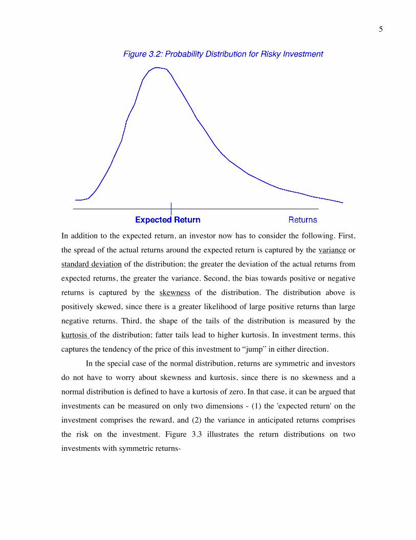
5

In addition to the expected return, an investor now has to consider the following. First,

the spread of the actual returns around the expected return is captured by the variance or

standard deviation of the distribution; the greater the deviation of the actual returns from

expected returns, the greater the variance. Second, the bias towards positive or negative

returns is captured by the skewness of the distribution. The distribution above is

positively skewed, since there is a greater likelihood of large positive returns than large

negative returns. Third, the shape of the tails of the distribution is measured by the

kurtosis of the distribution; fatter tails lead to higher kurtosis. In investment terms, this

captures the tendency of the price of this investment to “jump” in either direction.

In the special case of the normal distribution, returns are symmetric and investors

do not have to worry about skewness and kurtosis, since there is no skewness and a

normal distribution is defined to have a kurtosis of zero. In that case, it can be argued that

investments can be measured on only two dimensions - (1) the 'expected return' on the

investment comprises the reward, and (2) the variance in anticipated returns comprises

the risk on the investment. Figure 3.3 illustrates the return distributions on two

investments with symmetric returns-

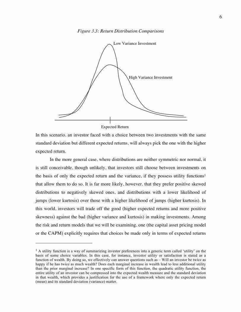
6

Figure 3.3: Return Distribution Comparisons

Expected Return

Low Variance Investment

High Variance Investment

In this scenario, an investor faced with a choice between two investments with the same

standard deviation but different expected returns, will always pick the one with the higher

expected return.

In the more general case, where distributions are neither symmetric nor normal, it

is still conceivable, though unlikely, that investors still choose between investments on

the basis of only the expected return and the variance, if they possess utility functions1

that allow them to do so. It is far more likely, however, that they prefer positive skewed

distributions to negatively skewed ones, and distributions with a lower likelihood of

jumps (lower kurtosis) over those with a higher likelihood of jumps (higher kurtosis). In

this world, investors will trade off the good (higher expected returns and more positive

skewness) against the bad (higher variance and kurtosis) in making investments. Among

the risk and return models that we will be examining, one (the capital asset pricing model

or the CAPM) explicitly requires that choices be made only in terms of expected returns

1 A utility function is a way of summarizing investor preferences into a generic term called ‘utility’ on the basis of some choice variables. In this case, for instance, investor utility or satisfaction is stated as a function of wealth. By doing so, we effectively can answer questions such as – Will an investor be twice as happy if he has twice as much wealth? Does each marginal increase in wealth lead to less additional utility than the prior marginal increase? In one specific form of this function, the quadratic utility function, the entire utility of an investor can be compressed into the expected wealth measure and the standard deviation in that wealth, which provides a justification for the use of a framework where only the expected return (mean) and its standard deviation (variance) matter.

7

and variances. While it does ignore the skewness and kurtosis, it is not clear how much of

a factor these additional moments of the distribution are in determining expected returns.

In closing, we should note that the return moments that we run into in practice are

almost always estimated using past returns rather than future returns. The assumption we

are making when we use historical variances is that past return distributions are good

indicators of future return distributions. When this assumption is violated, as is the case

when the asset’s characteristics have changed significantly over time, the historical

estimates may not be good measures of risk.

: 3.1: Do you live in a mean-variance world? Assume that you had to pick between two investments. They have the same

expected return of 15% and the same standard deviation of 25%; however, investment A

offers a very small possibility that you could quadruple your money, while investment

B’s highest possible payoff is a 60% return. Would you

a. be indifferent between the two investments, since they have the same expected return

and standard deviation?

b. prefer investment A, because of the possibility of a high payoff?

c. prefer investment B, because it is safer?

Risk Assessment: A Behavioral Perspective

The mean-variance framework for assessing risk is focused on measuring risk

quantitatively, often with one number – a standard deviation. While this focus is

understandable, because it introduces discipline into the process and makes it easier for

us to follow up and measure expected returns, it may not fully capture the complicated

relationship that we, as human beings, have with risk. Behavioral finance scholars present

three aspects of risk assessment that are at variance with the men-variance school’s view

of risk:

a. Loss aversion: In experiments with human subjects, there is evidence that individuals

are affected far more negatively by a loss than they are helped by an equivalent gain,

and that they generally measure losses in dollar terms rather than percentage terms.

Put another way, investors are loss averse rather than risk averse. Consequently,

8

investments where there is even a small chance of a significant loss in wealth will be

viewed as risky, even if they have only a small standard deviation.

b. Familiarity bias: Individuals seem to perceive less risk with investments that they are

familiar with than with unfamiliar investments. Thus, they see less risk in a domestic

company with a long provenance than they do in an emerging market firm. This may

explain why there is a “home bias” in portfolios, where investors over invest in

investments in their domestic market and under invest in foreign investments. In an

extension of this bias, the risk that individuals perceive in an activity or investment is

inversely proportional to the difficulty they face in understanding it.

c. Emotional factors: There is an emotional component to risk that quantitative risk

measures cannot capture. This component can have both a positive affect, where

gains accentuate positive affects (happiness and optimism) and losses feed into

negative affects (worry and anxiety). More generally, investor moods can affect risk

perceptions, with investments that are viewed as relatively safe in buoyant times

becoming risky when investor moods shift.

In recent years, there have been attempts to build composite risk measures that bring

these behavioral components into the analysis. While no consensus has emerged, it may

explain why quantitative measures of risk (such as standard deviation) for firm may

deviate from the many qualitative risk measures that often exist for the same firm.

Illustration 3.1: Calculation of standard deviation using historical returns: Disney

We collected the data on the returns we would have made on a monthly basis for

every month from January 2004 to December 2008 on an investment in Disney stock. To

compute the returns, we looked at the price change in each month (with Pricet being the

price at the end of month t) and dividends if any during the month (Dividendst):

€

Returnt =(Pricet - Pricet -1 + Dividendst )

Pricet -1

The monthly returns are graphed in figure 3.4:

9

Disney’s returns reflect the risk that an investor in the stock would have faced over the

period, with October 2004 being the best month (with a return of 11.82%) and October

2008 representing the worst month (with a return of -15.58%).

Looking at the summary statistics, the average monthly return on Disney over the

59 months was 0.18%. In fact, we started the period, in January 2004, with a stock price

of $23.68 and ended the period on December 31, 2008 with a stock price of $22.69

However, the stock did pay an annual dividend that increased from $0.24 in 2004 to

$0.35 in 2008. To measure the volatility or risk in the stock, we estimated the standard

deviation in monthly returns over this period to be 5.59%; the variance in monthly returns

was 31.25%.2 To convert monthly values to annualized ones:

Annualized Standard Deviation = 5.59% *√12 = 19.36%

Annualized Variance = 31.25% * 12 = 374.98%2

2 The variance is percent squared. In other words, if you stated the standard deviation of 9.96% in decimal terms, it would be 0.0996 but the variance of 99.15% would be 0.009915 in decimal terms.

10

Without making comparisons to the standard deviations in stock returns of other

companies, we cannot really draw any conclusions about the relative risk of Disney by

just looking at its standard deviation.

optvar.xls is a dataset on the web that summarizes average standard deviations

of equity values by industry group in the United States.

3.2. Upside and Downside Risk You are looking at the historical standard deviations over the last 5 years on two

investments. Both have standard deviations of 35% in returns during the period, but one

had a return of -10% during the period, whereas the other had a return of +40% during

the period. Would you view them as equally risky?

a. Yes

b. No

Why do we not differentiate between “upside risk” and “downside risk” in finance?

In Practice: Estimating only downside risk

The variance of a return distribution measures the deviation of actual returns from

the expected return. In estimating the variance, we consider not only actual returns that

fall below the average return (downside risk) but also those that lie above it (upside risk).

As investors, it is the downside that we generally consider as risk. There is an alternative

measure called the semi-variance that considers only downside risk. To estimate the

semi-variance, we calculate the deviations of actual returns from the average return only

if the actual return is less than the expected return; we ignore actual returns that are

higher than the average return.

Semi-variance =

€

(Rt−Average Return)2

nt=1

t= n

∑

n = number of periods where actual return < Average return

With a normal distribution, the semi-variance will generate a value identical to the

variance, but for any non-symmetric distribution, the semi-variance will yield different

values than the variance. In general, a stock that generates small positive returns in most

11

periods but very large negative returns in a few periods will have a semi-variance that is

much higher than the variance.

II. Rewarded and Unrewarded Risk Risk, as we have defined it in the previous section, arises from the deviation of

actual returns from expected returns. This deviation, however, can occur for any number

of reasons, and these reasons can be classified into two categories - those that are specific

to the investment being considered (called firm specific risks) and those that apply across

most or all investments (market risks).

The Components of Risk

When a firm makes an investment, in a new asset or a project, the return on that

investment can be affected by several variables, most of which are not under the direct

control of the firm. Some of the risk comes directly from the investment, a portion from

competition, some from shifts in the industry, some from changes in exchange rates and

some from macroeconomic factors. A portion of this risk, however, will be eliminated by

the firm itself over the course of multiple investments and another portion by investors as

they hold diversified portfolios.

The first source of risk is project-specific;

an individual project may have higher or lower

cashflows than expected, either because the firm

misestimated the cashflows for that project or

because of factors specific to that project. When

firms take a large number of similar projects, it

can be argued that much of this risk should be diversified away in the normal course of

business. For instance, Disney, while considering making a new movie, exposes itself to

estimation error - it may under or over estimate the cost and time of making the movie,

and may also err in its estimates of revenues from both theatrical release and the sale of

merchandise. Since Disney releases several movies a year, it can be argued that some or

Project Risk: This is risk that affects

only the project under consideration, and

may arise from factors specific to the

project or estimation error.

12

much of this risk should be diversifiable across movies produced during the course of the

year.3

The second source of risk is

competitive risk, whereby the earnings

and cashflows on a project are affected

(positively or negatively) by the actions

of competitors. While a good project analysis will build in the expected reactions of

competitors into estimates of profit margins and growth, the actual actions taken by

competitors may differ from these expectations. In most cases, this component of risk

will affect more than one project, and is therefore more difficult to diversify away in the

normal course of business by the firm. Disney, for instance, in its analysis of revenues

from its theme parks division may err in its assessments of the strength and strategies of

competitors like Universal Studios. While Disney cannot diversify away its competitive

risk, stockholders in Disney can, if they are willing to hold stock in the competitors.4

The third source of risk is industry-specific risk –– those factors that impact the

earnings and cashflows of a specific industry. There are three sources of industry-specific

risk. The first is technology risk, which reflects the effects of technologies that change or

evolve in ways different from those expected when a project was originally analyzed. The

second source is legal risk, which reflects the effect of changing laws and regulations.

The third is commodity risk, which reflects

the effects of price changes in commodities

and services that are used or produced

disproportionately by a specific industry.

Disney, for instance, in assessing the

prospects of its broadcasting division

(ABC) is likely to be exposed to all three risks; to technology risk, as the lines between

television entertainment and the internet are increasing blurred by companies like

3 To provide an illustration, Disney released Treasure Planet, an animated movie, in 2002, which cost $140 million to make and resulted in a $98 million write-off. A few months later, Finding Nemo, another animated Disney movie made hundreds of millions of dollars and became one of the biggest hits of 2003.

Competitive Risk: This is the unanticipated

effect on the cashflows in a project of competitor

actions - these effects can be positive or negative.

Industry-Specific Risk: These are unanticipated

effects on project cashflows of industry-wide

shifts in technology, changes in laws or in the

price of a commodity.

13

Microsoft, to legal risk, as the laws governing broadcasting change and to commodity

risk, as the costs of making new television programs change over time. A firm cannot

diversify away its industry-specific risk without diversifying across industries, either with

new projects or through acquisitions. Stockholders in the firm should be able to diversify

away industry-specific risk by holding portfolios of stocks from different industries.

The fourth source of risk is international risk. A firm faces this type of risk when

it generates revenues or has costs outside its domestic market. In such cases, the earnings

and cashflows will be affected by unexpected

exchange rate movements or by political

developments. Disney, for instance, is clearly

exposed to this risk with its theme park in

Hong Kong. Some of this risk may be

diversified away by the firm in the normal course of business by investing in projects in

different countries whose currencies may not all move in the same direction. McDonalds,

for instance, operates in many different countries and should be able to diversify away

some (though not all) of its exposure to international risk. Companies can also reduce

their exposure to the exchange rate component of this risk by borrowing in the local

currency to fund projects. Investors should be able to reduce their exposure to

international risk by diversifying globally.

The final source of risk is market risk: macroeconomic factors that affect

essentially all companies and all projects, to varying degrees. For example, changes in

interest rates will affect the value of projects already taken and those yet to be taken both

directly, through the discount rates, and indirectly, through the cashflows. Other factors

that affect all investments include the term structure (the difference between short and

long term rates), the risk preferences of

investors (as investors become more risk

averse, more risky investments will lose value),

inflation, and economic growth. While expected

4 Firms could conceivably diversify away competitive risk by acquiring their existing competitors. Doing so would expose them to attacks under the anti-trust law, however and would not eliminate the risk from as yet unannounced competitors.

International Risk: This is the additional

uncertainty created in cashflows of projects by

unanticipated changes in exchange rates and by

political risk in foreign markets.

Market Risk: Market risk refers to the

unanticipated changes in project cashflows

created by changes in interest rates, inflation

rates and the economy that affect all firms,

though to differing degrees.

14

values of all these variables enter into project analysis, unexpected changes in these

variables will affect the values of these investments. Neither investors nor firms can

diversify away this risk since all risky investments bear some exposure to this risk.

: 3.3. Risk is in the eyes of the beholder A privately owned firm will generally end up with a higher discount rate for a project

than would an otherwise similar publicly traded firm with diversified investors.

a. True

b. False

Does this provide a rationale for why a private firm may be acquired by a publicly traded

firm?

Why Diversification Reduces or Eliminates Firm-Specific Risk

Why do we distinguish between the different types of risk? Risk that affect one of

a few firms, i.e., firm specific risk, can be reduced or even eliminated by investors as they

hold more diverse portfolios due to two reasons.

• The first is that each investment in a

diversified portfolio is a much smaller

percentage of that portfolio. Thus, any risk

that increases or reduces the value of only that

investment or a small group of investments

will have only a small impact on the overall portfolio.

• The second is that the effects of firm-specific actions on the prices of individual

assets in a portfolio can be either positive or negative for each asset for any

period. Thus, in large portfolios, it can be reasonably argued that this risk will

average out to be zero and thus not impact the overall value of the portfolio.

In contrast, risk that affects most of all assets in the market will continue to persist even

in large and diversified portfolios. For instance, other things being equal, an increase in

interest rates will lower the values of most assets in a portfolio. Figure 3.5 summarizes

the different components of risk and the actions that can be taken by the firm and its

investors to reduce or eliminate this risk.

Diversification: This is the process of

holding many investments in a

portfolio, either across the same asset

class (eg. stocks) or across asset

classes (real estate, bonds etc.

15

Actions/Risk that affect only one firm

Actions/Risk that affect all investments

Firm-specific Market

Projects maydo better orworse thanexpected

Competitionmay be strongeror weaker thananticipated

Entire Sectormay be affectedby action

Exchange rateand Politicalrisk

Interest rate,Inflation & news about economy

Figure 3.5: A Break Down of Risk

Affects fewfirms

Affects manyfirms

Firm can reduce by

Investing in lots of projects

Acquiring competitors

Diversifying across sectors

Diversifying across countries

Cannot affect

Investors can mitigate by

Diversifying across domestic stocks Diversifying across asset classes

Diversifying globally

While the intuition for diversification reducing risk is simple, the benefits of

diversification can also be shown statistically. In the last section, we introduced standard

deviation as the measure of risk in an investment and calculated the standard deviation

for an individual stock (Disney). When you combine two investments that do not move

together in a portfolio, the standard deviation of that portfolio can be lower than the

standard deviation of the individual stocks in the portfolio. To see how the magic of

diversification works, consider a portfolio of two assets. Asset A has an expected return

of µA and a variance in returns of σ2A, while asset B has an expected return of µB and a

variance in returns of σ2B. The correlation in returns between the two assets, which

measures how the assets move together, is ρAB.5 The expected returns and variance of a

two-asset portfolio can be written as a function of these inputs and the proportion of the

portfolio going to each asset.

µportfolio = wA µA + (1 - wA) µB

σ2portfolio = wA2 σ2A + (1 - wA)2 σ2B + 2 wA wB ρΑΒ σA σB

where

16

wA = Proportion of the portfolio in asset A

The last term in the variance formulation is sometimes written in terms of the covariance

in returns between the two assets, which is

σAB = ρΑΒ σA σB

The savings that accrue from diversification are a function of the correlation coefficient.

Other things remaining equal, the higher the correlation in returns between the two assets,

the smaller are the potential benefits from diversification. The following example

illustrates the savings from diversification.

Under Diversification: A Behavioral Perspective

The argument that investors should diversify is impeccable, at least in a mean-

variance world full of rational investors. The reality, though, is that most investors do not

diversify. In one of the earliest studies of this phenomenon, Blume, Crockett and Friend

(1974) examined the portfolios of individual investors and reported that 34% of the

investors held only one dividend paying stock in their portfolios, 55% held between one

and ten stocks and that only 11% held more than 10 stocks. While these investors could

be granted the excuse that mutual funds were neither as prevalent nor as accessible as

they are today, Goetzmann and Kumar looked at 60,000 investors at a discount brokerage

house between 1991 and 1996 and conclude that there has been little improvement on the

diversification front, and that the absence of diversification cannot be explained away

easily with transactions costs.6 While some researchers have tried to find explanations

within the conventional finance framework, behavioral economists offer three possible

reasons:

a. The Gambling instinct: One possible explanation is that investors construct their

portfolios, as layered pyramids, with the bottom layer designed for downside

protection and the top layer for risk seeking and upside potential. Investing in one or

5 The correlation is a number between –1 and +1. If the correlation is –1, the two stocks move in lock step but in opposite directions. If the correlation is +1, the two stocks move together in synch. 6 Geotzmann, W.N. and A. Kumar, 2008, Equity Portfolio Diversification, Review of Finance. V12, 433-463. They find that 25% of investors hold only one stock and 50% of investors hold two or three stocks in their portfolios.

17

a few stocks in the top layer may not yield efficient risk taking portfolios, but they

offer more upside. In a sense, these investments are closer to lottery tickets than to

financial investments.7

b. Over confidence: Goetzmann and Kumar note that investors who overweight specific

industries or stock characteristics such as volatility tend to be less diversified than

investors who hold wider portfolios. They argue that this is consistent with investors

being over confident in their own abilities to find winners and thus not diversifying.

c. Narrow framing and estimation biases: Investors who frame their investment

decisions narrowly (looking at pieces of their portfolio rather than the whole) or

misestimate correlations (by assuming that individual stocks are more highly

correlated with each other than they really are) will hold less diversified portfolios.

In summary, many individual investors and some institutional investors seem to ignore

the lessons of diversification and choose to hold narrow portfolios. Their perspective on

risk may vary from more diversified investors in the same companies.

Illustration 3.2: Variance of a portfolio: Disney and Aracruz ADR

In illustration 3.1, we computed the average return and standard deviation of

returns on Disney between January 2004 and December 2008. While Aracruz is a

Brazilian stock, it has been listed and traded as an American Depository Receipt (ADR)

in the U.S. market over the same period. 8 Using the same 60 months of data on Aracruz,

we computed the average return and standard deviation on its returns over the same

period:

Disney Aracruz ADR

Average Monthly Return 0.18% -0.74%

Standard Deviation in Monthly Returns 5.59% 14.87%

Between 2004 and 2008, Disney generated higher returns than Aracruz, with lower

volatility. With the benefit of hindsight, Disney would have been a much better

7 Shefrin, H. and M. Statman, 2000, Behavioral Portfolio Theory, Journal of Financial and Quantitative Analysis, v35, pp 127-151. 8 Like most foreign stocks, Aracruz has a listing for depository receipts or ADRs on the U.S. exchanges. Effectively, a bank buys shares of Aracruz in Brazil and issues dollar denominated shares in the United

18

investment than Aracruz, at least over this period. There are two points worth making.

The first is that Aracruz generated an average monthly return of 2.47% from January

2004 to April 2008; the stock price dropped from an all time high of $90.74 to $8.39

between May and December of 2008. The second is that these returns were on the

Aracruz ADR and thus in dollar terms. These returns are therefore affected both by the

stock price performance of Aracruz (in Brazilian Reals(BR)) and the $/BR exchange rate.

A contributing factor to decline in the ADR price in the latter part of 2008 was the

precipitous fall in the value of the BR, relative to the dollar.

To examine how a combination of Disney and the Aracruz ADR would do as an

investment, we computed the correlation between the two stocks over the 60-month

period to be 0.1807. Consider now a portfolio that is invested 90% in Disney and 10% in

the Aracruz ADR. The variance and the standard deviation of the portfolio can be

computed as follows:

Variance of portfolio = wDis2 σ2Dis + (1 - wDis)2 σ2Ara + 2 wDis wAra ρDis,Ara σDis σAra

= (.9)2(.0559)2+(.1)2(.1487)2+ 2 (.9)(.1)(.1807)(.0559)(.1487)

=.003023

Standard Deviation of Portfolio =

€

.003023 = .0550 or 5.50%

The portfolio is less risky than either of the two stocks that go into it. In figure 3.6, we

graph the standard deviation in the portfolio as a function of the proportion of the

portfolio invested in Disney:

States to interested investors. Aracruz’s ADR price tracks the price of the local listing while reflecting exchange rate changes.

19

As the proportion of the portfolio invested in Aracruz shifts towards 100%, the standard

deviation of the portfolio converges on the standard deviation of Aracruz.

Aracruz’s travails between May and December of 2008 also provide some insight

into the essence of firm specific and market risk. The company had reported healthy

profits from 2004 through 2007 but some of those profits came from managers

speculating with derivatives (options and futures) that the Brazilian Real would continue

to strengthen against the U.S. dollar. When the tide turned in 2008, and the Brazilian Real

started weakening, the derivative bets made by the firm generated losses in excess of $ 2

billion, which, in turn caused the drop in the stock price. The global market collapse in

the last three months of the year accelerated the fall. The speculative losses from

exchange rate bets are clearly firm specific risk but the losses accruing from the global

crisis can be attributed to market risk.

Identifying the Marginal Investor

The marginal investor in a firm is the investor who is most likely to be trading at

the margin and therefore has the most influence on the pricing of its equity. In some

20

cases, this may be a large institutional investor, but institutional investors themselves can

differ in several ways. The institution may be a taxable mutual fund or a tax-exempt

pension fund, may be domestically or internationally diversified, and vary on investment

philosophy. In some cases, the marginal investors may be individuals, and here again

there can be wide differences depending upon how diversified these individuals are, and

what their investment objectives may be. In still other cases, the marginal investors may

be insiders in the firm who own a significant portion of the equity of the firm and are

involved in the management of the firm.

While it is difficult to identify the marginal investor in a firm, we would begin by

breaking down the percent of the firm’s stock held by individuals, institutions and

insiders in the firm. This information, which is available widely for US stocks, can then

be analyzed to yield the following conclusions:

• If the firm has relatively small institutional holdings but substantial holdings by

wealthy individual investors, the marginal investor is an individual investor with a

significant equity holding in the firm. In this case, we have to consider how

diversified that individual investor’s portfolio is to assess project risk. If the

individual investor is not diversified, this firm may have to be treated like a private

firm, and the cost of equity has to include a premium for all risk, rather than just non-

diversifiable risk. If on the other hand, the individual investor is a wealthy individual

with significant stakes in a large number of firms, a large portion of the risk may be

diversifiable.

• If the firm has small institutional holdings and small insider holdings, its stock is held

by large numbers of individual investors with small equity holdings. In this case, the

marginal investor is an individual investor, with a portfolio that may be only partially

diversified. For instance, phone and utility stocks in the United States, at least until

recently, had holdings dispersed among thousands of individual investors, who held

the stocks for their high dividends. This preference for dividends meant, however,

that these investors diversified across only those sectors where firms paid high

dividends.

• If the firm has significant institutional holdings and small insider holdings, the

marginal investor is almost always a diversified, institutional investor. In fact, we can

21

learn more about what kind of institutional investor holds stock by examining the top

15 or 20 largest stockholders in the firms, and then categorizing them by tax status

(mutual funds versus pension funds), investment objective (growth or value) and

globalization (domestic versus international).

• If the firm has significant institutional holdings and large insider holdings, the choice

for marginal investor becomes a little more complicated. Often, in these scenarios, the

large insider is the founder or original owner for the firm, and often, this investor

continues to be involved in the top management of firm. Microsoft and Dell are good

examples, with Bill Gates and Michael Dell being the largest stockholders in the

firms. In most of these cases, however, the insider owner seldom trades the stock, and

his or her wealth is determined by the level of the stock price, which is determined by

institutional investors trading the stock. We would argue that the institutional investor

is the marginal investor in these firms as well, though the leading stockholder will

influence the final decision.

Thus, by examining the percent of stock held by different groups, and the largest

investors in a firm, we should have a sense of who the marginal investor in the firm is,

and how best to assess and risk in corporate financial analysis.

Why do we care about the marginal investor? Since the marginal investors are

assumed to set prices, their assessments of risk should govern how the rest of us think

about risk. Thus, if the marginal investors are diversified institution, the only risk that

they see in a company is the risk that they cannot diversify away and managers at the

firm should be considering only that risk, when making investments. If the marginal

investors are undiversified individuals, they will care about all risk in a company and the

firm should therefore consider all risk, when making investments.

Illustration 3.3: Identifying the Marginal Investor

Who are the marginal investors in Disney, Aracruz, Tata Chemicals and Deutsche

Bank? We begin to answer this question by examining whether insiders own a significant

portion of the equity in the firm and are involved in the top management of the firm.

Although no such investors exist at Deutsche Bank, there are significant insider holdings

at the other three companies:

22

• While the shares held by the Disney family have dwindled to less than 1%, Disney’s

acquisition of Pixar has resulted in Steve Jobs becoming the largest single stockholder

in the company, owning about 7% of the stock in the company.

• At Ararcuz, the voting shares are held by the Votorantim Group (84%) and the

Brazilian National Development Bank (BNDES), while the non-voting shares are

held by a mix of institutional and individual investors.

• At Tata Chemicals, the Tata family control (even if they might not hold) a significant

portion of the stock through other Tata companies in the group.

However, we do not believe that insiders represent the marginal investors at any of these

companies because their holdings are static for two reasons. One is that their capacity to

trade is restricted as insiders, especially in the case of Disney.9 The other is that trading

may result in loss of the control they exercise over the firm, at least at Tata Chemicals

and Aracruz. Consequently, we examine the proportion of stock held in each of the firms

by individuals, insiders and institutions, in table 3.1.

Table 3.1: Investors in Disney, Aracruz, Deutsche Bank and Tata Chemicals

Disney Deutsche Bank Aracruz (non-voting) Tata Chemicals Institutions 72% 76% 32% 47% Individuals 21% 23% 60% 24% Insiders 7% 1% 8% 29%* Source: Value Line, Morningstar, Bloomberg.

All four companies are widely held by institutional investors, and foreign institutional

investors hold significant portions of Aracruz and Tata Chemicals. In table 3.2, we

examine the ten largest investors in each firm at the end of 2008 in Table 8.5, with the

percent of the firm’s stock held by each (in brackets).

Table 3.2: Largest Stockholders in Disney, Deutsche Bank and Tata Chemicals

Disney Deutsche Bank Aracruz Preferred –Tata Chemicals Steven Jobs (7.43%) Deutsche Post

(8.05%) BB DTVM (0.89%) Tata Sons (14.26%)

Fidelity (4.86%) Allianz (6.81%) Barclays(0.34%) Life Insurance Co (11.71%)

State Street (3.97%) AXA (4.64%) Banco Itau (0.32%) Tata Investment (6.8%) Barclays (3.79%) Credit Suisse (3.55%) Banco Barclays (0.19%) Tata Tea (6.54%) Vanguard Group (3.07%) Deutsche Bank Vanguard Group (0.18%) New India Assur. 9 Insider trading laws in the United States restrict insiders from trading on material information and also require filings of any trades that are made.

23

(3.52%) (2.58%) Southeastern Asset (2.40%)

Barclays (3.02%) UBS Strategy (0.17%) Hindustan Lever (2.14%)

State Farm Mutual (2.27%)

Blackrock (2.35%) Banco Itau (0.17%) General Insurance (2.12%)

AXA (2.13%) UBS (1.65%) Dimensional Fund (0.10%)

United India Insur. (1.13%)

Wellington Mgmt (1.87%)

Deka (1.52%) Banco Bradesco (0.09%) National Insurance (1.01%)

Massachusetts Finl (1.57%)

Dekabank (1.44%) Landesbank (0.08%) Templeton Funds (1.01%)

Source: Bloomberg

Nine of the ten largest investors in Disney are institutional investors, suggesting that we

are on safe grounds assuming that the marginal investor in Disney is likely to be both

institutional and diversified. The two largest investors in Deutsche Bank are Allianz, the

German insurance giant, and Deutsche Post, the privatized German postal company,

reflecting again the cross-holding corporate governance structure favored by German

corporations. However, the investors below Allianz are all institutional investors, and

about half of them are non-German. Here again, we can safely assume that the marginal

investor is likely to be institutional and broadly diversified across at least European

equities rather than just German stocks. The common shares in Aracruz, where the voting

rights reside, is held by a handful of controlling stockholders, but trading in this stock is

light. The preferred shares are widely dispersed among a mix of domestic and

international institutional investors. While there is a clear danger here that the company

will be run for the benefit of the voting shareholders, the price of the voting stock is

closely linked to the price of the preferred shares. Self-interest alone should induce the

voting shareholders to consider the investors in the preferred shares as the marginal

investors in the company. Finally, with Tata Chemicals, four of the ten largest investors

are other Tata companies and those holdings are seldom traded. All of the remaining

large investors are institutional investors, with about 12% of the stock held by foreign

institutional investors.

In summary, then, we are on very safe ground with Disney and Deutsche Bank,

when we assume that only the risk that cannot be diversified away should be considered

when the company makes investments. We are on less secure ground with Aracruz and

Tata Chemicals, because of the heavy influence of insiders, but we feel that institutional

24

investors exercise enough influence on how equity is priced at both firms for us to make

the same assumption.

Why is the marginal investor assumed to be diversified?

The argument that investors can reduce their exposure to risk by diversifying can

be easily made, but risk and return models in finance go further. They argue that the

marginal investor, who sets prices for investments, is well diversified; thus, the only risk

that will be priced in the risk as perceived by that investor. The justification that can be

offered is a simple one. The risk in an investment will always be perceived to be higher

for an undiversified investor than to a diversified one, since the latter does not consider

any firm-specific risk while the former does. If both investors have the same perceptions

about future earnings and cashflows on an asset, the diversified investor will be willing to

pay a higher price for that asset because of his or her risk perceptions. Consequently, the

asset, over time, will end up being held by diversified investors.

While this argument is a powerful one for stocks and other assets, which are

traded in small units and are liquid, it is less so for investments that are large and illiquid.

Real estate in most countries is still held by investors who are undiversified and have the

bulk of their wealth tied up in these investments. The benefits of diversification are

strong enough, however, that securities such as real estate investment trusts and

mortgage-backed bonds were created to allow investors to invest in real estate and stay

diversified at the same time.

Note that diversification does not require investors to give up their pursuit of

higher returns. Investors can be diversified and try to beat the market at the same time,

For instance, investors who believe that they can do better than the market by buying

stocks trading at low PE ratios can still diversify by holding low PE stocks in a number of

different sectors at the same time.

: 3.4. Management Quality and Risk A well managed firm is less risky than a firm that is badly managed.

a. True

b. False

25

In Practice: Who should diversify? The Firm or Investors?

As we noted in the last section, the exposure to each type of risk can be mitigated

by either the firm or by investors in the firm. The question of who should do it can be

answered fairly easily by comparing the costs faced by each. As a general rule, a firm

should embark on actions that reduce risk only if it is cheaper for it to do so than it is for

its investors. With a publicly traded firm, it will usually be much cheaper for investors to

diversify away risk than it is for the firm. Consider, for instance, risk that affects an entire

sector. A firm can reduce its exposure to this risk by either acquiring other firms, paying

large premiums over the market price, or by investing large amounts in businesses where

it does not have any expertise. Investors in the firm, on the other hand, can accomplish

the same by expanding their portfolios to include stocks in other sectors or even more

simply by holding diversified mutual funds. Since the cost of diversifying for investors is

very low, firms should try to diversify away risk only if the cost is minimal or if the risk

reduction is a side benefit from an action with a different objective. One example would

be project risk. Since Disney is in the business of making movies, the risk reduction that

comes from making lots of movies is essentially costless.

The choice is more complicated for private businesses. The owners of these

businesses often have the bulk of their wealth invested in these businesses and they can

either try to take money out of the businesses and invest it elsewhere or they can diversify

their businesses. In fact, many family businesses in Latin America and Asia became

conglomerates as they expanded, partly because they wanted to spread their risks.

III. Measuring Market Risk

While most risk and return models in use in corporate finance agree on the first

two step of this process, i.e., that risk comes from the distribution of actual returns around

the expected return and that risk should be measured from the perspective of a marginal

investor who is well diversified, they part ways on how to measure the non-diversifiable

or market risk. In this section, we will provide a sense of how each of the four basic

models - the capital asset pricing model (CAPM), the arbitrage pricing model (APM) and

the multi-factor model - approaches the issue of measuring market risk.

26

A. The Capital Asset Pricing Model

The risk and return model that has been in use the longest and is still the standard

in most real world analyses is the capital asset pricing model (CAPM). While it has come

in for its fair share of criticism over the years, it provides a useful starting point for our

discussion of risk and return models.

1. Assumptions

While diversification has its attractions in terms

of reducing the exposure of investors to firm specific

risk, most investors limit their diversification to

holding relatively few assets. Even large mutual funds

are reluctant to hold more than a few hundred stocks, and many of them hold as few as 10

to 20 stocks. There are two reasons for this reluctance. The first is that the marginal

benefits of diversification become smaller as the portfolio gets more diversified - the

twenty-first asset added will generally provide a much smaller reduction in firm specific

risk than the fifth asset added, and may not cover the marginal costs of diversification,

which include transactions and monitoring costs. The second is that many investors (and

funds) believe that they can find under valued assets and thus choose not to hold those

assets that they believe to be correctly or over valued.

The capital asset pricing model assumes that there are no transactions costs, all

assets are traded and that investments are infinitely divisible (i.e., you can buy any

fraction of a unit of the asset). It also assumes that there is no private information and that

investors therefore cannot find under or over valued assets in the market place. By

making these assumptions, it eliminates the factors that cause investors to stop

diversifying. With these assumptions in place, the logical end limit of diversification is to

hold every traded risky asset (stocks, bonds and real assets included) in your portfolio, in

proportion to their market value10. This portfolio of every traded risky asset in the market

place is called the market portfolio.

10 If investments are not held in proportion to their market value, investors are still losing some diversification benefits. Since there is no gain from over weighting some sectors and under weighting others in a market place where the odds are random of finding under valued and over valued assets, investors will not do so.

Riskless Asset: A riskless asset is

one, where the actual return is

always equal to the expected return.

27

2. Implications for Investors

If every investor in the market holds the same market portfolio, how exactly do

investors reflect their risk aversion in their investments? In the capital asset pricing

model, investors adjust for their risk preferences in their allocation decisions, where they

decide how much to invest in an asset with guaranteed returns – a riskless asset - and how

much in risky assets (market portfolio). Investors who are risk averse might choose to put

much or even all of their wealth in the riskless asset. Investors who want to take more

risk will invest the bulk or even all of their wealth in the market portfolio. Those

investors who invest all their wealth in the market portfolio and are still desirous of

taking on more risk, would do so by borrowing at the riskless rate and investing in the

same market portfolio as everyone else.

These results are predicated on two additional assumptions. First, there exists a

riskless asset. Second, investors can lend and borrow at this riskless rate to arrive at their

optimal allocations. There are variations of the CAPM that allow these assumptions to be

relaxed and still arrive at conclusions that are consistent with the general model.

: 3.5. Efficient Risk Taking In the capital asset pricing model, the most efficient way to take a lot of risk is to

a. Buy a well-balanced portfolio of the riskiest stocks in the market

b. Buy risky stocks that are also undervalued

c. Borrow money and buy a well diversified portfolio

3. Measuring the Market Risk of an Individual Asset

The risk of any asset to an investor is the risk added on by that asset to the

investor’s overall portfolio. In the CAPM world, where all investors hold the market

portfolio, the risk of an individual asset to an investor will be the risk that this asset adds

on to the market portfolio. Intuitively, assets that move more with the market portfolio

will tend to be riskier than assets that move less, since the movements that are unrelated

to the market portfolio will not affect the overall value of the portfolio when an asset is

added on to the portfolio. Statistically, this added risk is measured by the covariance of

the asset with the market portfolio.

28

The covariance is a non-standardized measure of market risk; knowing that the

covariance of Disney with the Market Portfolio is 55% does not provide a clue as to

whether Disney is riskier or safer than the average asset. We therefore standardize the

risk measure by dividing the covariance of each asset with the market portfolio by the

variance of the market portfolio. This yields the beta of the asset:

Beta of an asset i =

€

Covariance of asset i with Market PortfolioVariance of the Market Portfolio

Since the covariance of the market portfolio with itself is its variance, the beta of the

market portfolio, and by extension, the average asset in it, is one. Assets that are riskier

than average (using this measure of risk) will have betas that exceed one and assets that

are safer than average will have betas that are lower than one . The riskless asset will

have a beta of zero.

4. Getting Expected Returns

The fact that every investor holds some

combination of the riskless asset and the market

portfolio leads to the next conclusion, which is that the

expected return on an asset is linearly related to the

beta of the asset. In particular, the expected return on an asset can be written as a function

of the risk-free rate and the beta of that asset;

Expected Return on asset i

= Rf + βi [E(Rm) - Rf]

= Risk-free rate + Beta of asset i * (Risk premium on market portfolio)

where,

E(Ri) = Expected Return on asset i

Rf = Risk-free Rate

E(Rm) = Expected Return on market portfolio

βi = Beta of asset i

To use the capital asset pricing model, we need three inputs. While we will look at the

estimation process in far more detail in the next chapter, each of these inputs is estimated

as follows:

Beta: The beta of any investment

in the CAPM is a standardized

measure of the risk that it adds to the

market portfolio.

29

• The riskless asset is defined to be an asset where the investor knows the expected

return with certainty for the time horizon of the analysis. Consequently, the riskless

rate used will vary depending upon whether the time period for the expected return is

one year, five years or ten years.

• The risk premium is the premium demanded by investors for investing in the market

portfolio, which includes all risky assets in the market, instead of investing in a

riskless asset. Thus, it does not relate to any individual risky asset but to risky assets

as a class.

• The beta, which we defined to be the covariance of the asset divided by the market

portfolio, is the only firm-specific input in this equation. In other words, the only

reason two investments have different expected returns in the capital asset pricing

model is because they have different betas.

In summary, in the capital asset pricing model all of the market risk is captured in one

beta, measured relative to a market portfolio, which at least in theory should include all

traded assets in the market place held in proportion to their market value.

: 3.6. What do negative betas mean? In the capital asset pricing model, there are assets that can have betas that are less than

zero. When this occurs, which of the following statements describes your investment?

a. This investment will have an expected return less than the riskless rate

b. This investment insures your “diversified portfolio” against some type of market risk

c. Holding this asset makes sense only if you are well diversified

d. All of the above

In Practice: Index Funds and Market Portfolios

Many critics of the capital asset pricing model seize on its conclusion that all

investors in the market will hold the market portfolio, which includes all assets in

proportion to their market value, as evidence that it is an unrealistic model. But is it? It is

true that not all assets in the world are traded and that there are transactions costs. It is

also true that investors sometimes trade on inside information and often hold

undiversified portfolios. However, we can create portfolios that closely resemble the

market portfolio using index funds. An index fund replicates an index by buying all of the

30

stocks in the index, in the same proportions that they form of the index. The earliest and

still the largest one is the Vanguard 500 Index fund, which replicates the S&P 500 index.

Today, we have access to index funds that replicate smaller companies in the United

States, European stocks, Latin American markets and Asian equities as well as bond and

commodity markets An investor can create a portfolio composed of a mix of index funds

– the weights on each fund should be based upon market values of the underlying market

- which resembles the market portfolio; the only asset class that is usually difficult to

replicate is real estate.

B. The Arbitrage Pricing Model

The restrictive assumptions in the capital asset pricing model and its dependence

upon the market portfolio have for long been viewed with skepticism by both academics

and practitioners. In the late seventies, an alternative and more general model for

measuring risk called the arbitrage pricing model was developed.11

1. Assumptions

The arbitrage pricing model is built on the

simple premise that two investments with the same

exposure to risk should be priced to earn the same

expected returns. An alternate way of saying this is that if two portfolios have the same

exposure to risk but offer different expected returns, investors can buy the portfolio that

has the higher expected returns and sell the one with lower expected returns, until the

expected returns converge.

Like the capital asset pricing model, the arbitrage pricing model begins by

breaking risk down into two components. The first is firm specific and covers

information that affects primarily the firm. The second is the market risk that affects all

investment; this would include unanticipated changes in a number of economic variables,

including gross national product, inflation, and interest rates. Incorporating this into the

return model above

11 Ross, Stephen A., 1976, The Arbitrage Theory Of Capital Asset Pricing, Journal of Economic Theory,

v13(3), 341-360.

Arbitrage: An investment that

requires no investment, involves no

risk but still delivers a sure profit.

31

R = E(R) + m + ε

where m is the market-wide component of unanticipated risk and ε is the firm-specific

component.

2. The Sources of Market-Wide Risk

While both the capital asset pricing model and the arbitrage pricing model make a

distinction between firm-specific and market-wide risk, they part ways when it comes to

measuring the market risk. The CAPM assumes that all of the market risk is captured in

the market portfolio, whereas the arbitrage pricing model allows for multiple sources of

market-wide risk, and measures the sensitivity of investments to each source with what a

factor betas. In general, the market component of unanticipated returns can be

decomposed into economic factors:

R = R + m + ε

= R + (β1 F1 + β2 F2 + .... +βn Fn) + ε

where

βj = Sensitivity of investment to unanticipated changes in factor j

Fj = Unanticipated changes in factor j

3. The Effects of Diversification

The benefits of diversification have been discussed extensively in our treatment of

the capital asset pricing model. The primary point of that discussion was that

diversification of investments into portfolios eliminate firm-specific risk. The arbitrage

pricing model makes the same point and concludes that the return on a portfolio will not

have a firm-specific component of unanticipated returns. The return on a portfolio can

then be written as the sum of two weighted averages -that of the anticipated returns in the

portfolio and that of the factor betas:

Rp = (w1R1+w2R2+...+wnRn)+ (w1β1,1+w2β1,2+...+wnβ1,n) F1 +

(w1β2,1+w2β2,2+...+wnβ2,n) F2 .....

where,

wj = Portfolio weight on asset j

Rj = Expected return on asset j

32

βi,j= Beta on factor i for asset j

Note that the firm specific component of returns (ε) in the individual firm equation

disappears in the portfolio as a result of diversification.

4. Expected Returns and Betas

The fact that the beta of a portfolio is the weighted average of the betas of the

assets in the portfolio, in conjunction with the absence of arbitrage, leads to the

conclusion that expected returns should be linearly related to betas. To see why, assume

that there is only one factor and that there are three portfolios. Portfolio A has a beta of

2.0, and an expected return on 20%; portfolio B has a beta of 1.0 and an expected return

of 12%; and portfolio C has a beta of 1.5, and an expected return on 14%. Note that the

investor can put half of his wealth in portfolio A and half in portfolio B and end up with a

portfolio with a beta of 1.5 and an expected return of 16%. Consequently no investor will

choose to hold portfolio C until the prices of assets in that portfolio drop and the expected

return increases to 16%. Alternatively, an investor can buy the combination of portfolio

A and B, with an expected return of 16%, and sell portfolio C with an expected return of

15%, and pure profit of 1% without taking any risk and investing any money. To prevent

this “arbitrage” from occurring, the expected returns on every portfolio should be a linear

function of the beta to prevent this f. This argument can be extended to multiple factors,

with the same results. Therefore, the expected return on an asset can be written as

E(R) = Rf + β1 [E(R1)-Rf] + β2 [E(R2)-Rf] ...+ βn [E(Rn)-Rf]

where

Rf = Expected return on a zero-beta portfolio

E(Rj) = Expected return on a portfolio with a factor beta of 1 for factor j, and zero

for all other factors.

The terms in the brackets can be considered to be risk premiums for each of the factors in

the model.

Note that the capital asset pricing model can be considered to be a special case of

the arbitrage pricing model, where there is only one economic factor driving market-wide

returns and the market portfolio is the factor.

E(R) = Rf + βm (E(Rm)-Rf)

33

5. The APM in Practice

The arbitrage pricing model requires estimates

of each of the factor betas and factor risk premiums in

addition to the riskless rate. In practice, these are

usually estimated using historical data on stocks and a

statistical technique called factor analysis. Intuitively, a factor analysis examines the

historical data looking for common patterns that affect broad groups of stocks (rather

than just one sector or a few stocks). It provides two output measures:

1. It specifies the number of common factors that affected the historical data that it

worked on.

2. It measures the beta of each investment relative to each of the common factors, and

provides an estimate of the actual risk premium earned by each factor.

The factor analysis does not, however, identify the factors in economic terms.

In summary, in the arbitrage-pricing model the market or non-diversifiable risk in

an investment is measured relative to multiple unspecified macro economic factors, with

the sensitivity of the investment relative to each factor being measured by a factor beta.

The number of factors, the factor betas and factor risk premiums can all be estimated

using a factor analysis.

C. Multi-factor Models for risk and return

The arbitrage pricing model's failure to identify specifically the factors in the

model may be a strength from a statistical standpoint, but it is a clear weakness from an

intuitive standpoint. The solution seems simple: Replace the unidentified statistical

factors with specified economic factors, and the resultant model should be intuitive while

still retaining much of the strength of the arbitrage pricing model. That is precisely what

multi-factor models do.

Deriving a Multi-Factor Model

Multi-factor models generally are not based on extensive economic rationale but

are determined by the data. Once the number of factors has been identified in the

arbitrage pricing model, the behavior of the factors over time can be extracted from the

data. These factor time series can then be compared to the time series of macroeconomic

Arbitrage: An investment

opportunity with no risk that earns a

return higher than the riskless rate.

34

variables to see if any of the variables are correlated, over time, with the identified

factors.

For instance, a study from the 1980s suggested

that the following macroeconomic variables were highly

correlated with the factors that come out of factor

analysis: industrial production, changes in the premium

paid on corporate bonds over the riskless rate, shifts in the term structure, unanticipated

inflation, and changes in the real rate of return.12 These variables can then be correlated

with returns to come up with a model of expected returns, with firm-specific betas

calculated relative to each variable. The equation for expected returns will take the

following form:

E(R) = Rf + βGNP (E(RGNP)-Rf) + βi (E(Ri)-Rf) ...+ βδ (E(Rδ)-Rf)

where

βGNP = Beta relative to changes in industrial production

E(RGNP) = Expected return on a portfolio with a beta of one on the industrial

production factor, and zero on all other factors

βi = Beta relative to changes in inflation

E(Ri) = Expected return on a portfolio with a beta of one on the inflation factor,

and zero on all other factors

The costs of going from the arbitrage pricing model to a macroeconomic multi-

factor model can be traced directly to the errors that can be made in identifying the

factors. The economic factors in the model can change over time, as will the risk

premium associated with each one. For instance, oil price changes were a significant

economic factor driving expected returns in the 1970s but are not as significant in other

time periods. Using the wrong factor(s) or missing a significant factor in a multi-factor

model can lead to inferior estimates of cost of equity.

In summary, multi factor models, like the arbitrage pricing model, assume that market

risk can be captured best using multiple macro economic factors and estimating betas

12 Chen, N., R. Roll and S.A. Ross, 1986, Economic Forces and the Stock Market, Journal of Business,

1986, v59, 383-404.

Unanticipated Inflation: This is

the difference between actual

inflation and expected inflation.

35

relative to each. Unlike the arbitrage pricing model, multi factor models do attempt to

identify the macro economic factors that drive market risk.

D. Proxy Models

All of the models described so far begin by thinking about market risk in

economic terms and then developing models that might best explain this market risk. All

of them, however, extract their risk parameters by looking at

historical data. There is a final class of risk and return

models that start with past returns on individual stocks, and

then work backwards by trying to explain differences in

returns across long time periods using firm characteristics.

In other words, these models try to find common characteristics shared by firms that have

historically earned higher returns and identify these characteristics as proxies for market

risk.

Fama and French, in a highly influential study of the capital asset pricing model

in the early 1990s, note that actual returns over long time periods have been highly

correlated with price/book value ratios and market capitalization.13 In particular, they

note that firms with small market capitalization and low price to book ratios earned

higher returns between 1963 and 1990. They suggest that these measures and similar ones

developed from the data be used as proxies for risk and that the regression coefficients be

used to estimate expected returns for investments. They report the following regression

for monthly returns on stocks on the NYSE, using data from 1963 to 1990:

Rt = 1.77% - 0.11 ln (MV) + 0.35 ln (BV/MV)

where

MV = Market Value of Equity

BV/MV = Book Value of Equity / Market Value of Equity

The values for market value of equity and book-price ratios for individual firms, when

plugged into this regression, should yield expected monthly returns. For instance, a firm

13 Fama, E.F. and K.R. French, 1992, The Cross-Section of Expected Returns, Journal of Finance, v47,

427-466.

Book-to-Market Ratio: This

is the ratio of the book value

of equity to the market value

of equity.

36

with a market value of $ 100 million and a book to market ratio of 0.5 would have an

expected monthly return of 1.02%.

Rt = 1.77% - 0.11 ln (100) + 0.35 ln (0.5) = 1.02%

As data on individual firms has becomes richer and more easily accessible in recent

years, these proxy models have expanded to include additional variables. In particular,

researchers have found that price momentum (the rate of increase in the stock price over

recent months) also seems to help explain returns; stocks with high price momentum tend

to have higher returns in following periods.

In summary, proxy models measure market risk using firm characteristics as

proxies for market risk, rather than the macro economic variables used by conventional

multi-factor models14. The firm characteristics are identified by looking at differences in

returns across investments over very long time periods and correlating with identifiable

characteristics of these investments.

A Comparative Analysis of Risk and Return Models

All the risk and return models developed in this chapter have common

ingredients. They all assume that only market-wide risk is rewarded, and they derive the

expected return as a function of measures of this risk. Figure 3.7 presents a comparison of

the different models:

14 Adding to the confusion, researchers in recent years have taken to describing proxy models also as multi factor models.

37

Figure 3.7: Competing Models for Risk and Return in Finance

The risk in an investment can be measured by the variance in actual returns around an expected return

E(R)

Riskless Investment Low Risk Investment High Risk Investment

E(R) E(R)

Risk that is specific to investment (Firm Specific) Risk that affects all investments (Market Risk)Can be diversified away in a diversified portfolio Cannot be diversified away since most assets1. each investment is a small proportion of portfolio are affected by it.2. risk averages out across investments in portfolioThe marginal investor is assumed to hold a “diversified” portfolio. Thus, only market risk will be rewarded and priced.

The CAPM The APM Multi-Factor Models Proxy ModelsIf there is 1. no private information2. no transactions costthe optimal diversified portfolio includes everytraded asset. Everyonewill hold this market portfolioMarket Risk = Risk added by any investment to the market portfolio:

If there are no arbitrage opportunities then the market risk ofany asset must be captured by betas relative to factors that affect all investments.Market Risk = Risk exposures of any asset to market factors

Beta of asset relative toMarket portfolio (froma regression)

Betas of asset relativeto unspecified marketfactors (from a factoranalysis)

Since market risk affectsmost or all investments,it must come from macro economic factors.Market Risk = Risk exposures of any asset to macro economic factors.

Betas of assets relativeto specified macroeconomic factors (froma regression)

In an efficient market,differences in returnsacross long periods mustbe due to market riskdifferences. Looking forvariables correlated withreturns should then give us proxies for this risk.Market Risk = Captured by the Proxy Variable(s)

Equation relating returns to proxy variables (from aregression)

Step 1: Defining Risk

Step 2: Differentiating between Rewarded and Unrewarded Risk

Step 3: Measuring Market Risk

The capital asset pricing model makes the most assumptions but arrives at the simplest

model, with only one risk factor requiring estimation. The arbitrage pricing model makes

fewer assumptions but arrives at a more complicated model, at least in terms of the

parameters that require estimation. In general, the CAPM has the advantage of being a

simpler model to estimate and to use, but it will under perform the richer multi factor

models when the company is sensitive to economic factors not well represented in the

market index. For instance, oil companies, which derive most of their risk from oil price

movements, tend to have low CAPM betas. Using a multi factor model, where one of the

factors may be capturing oil and other commodity price movements, will yield a better

estimate of risk and higher cost of equity for these firms15.

15 Weston, J.F. and T.E. Copeland, 1992, Managerial Finance, Dryden Press. They used both approaches to estimate the cost of equity for oil companies in 1989 and came up with 14.4% with the CAPM and 19.1% using the arbitrage pricing model.

38

The biggest intuitive block in using the arbitrage pricing model is its failure to

identify specifically the factors driving expected returns. While this may preserve the

flexibility of the model and reduce statistical problems in testing, it does make it difficult

to understand what the beta coefficients for a firm mean and how they will change as the

firm changes (or restructures).

Does the CAPM work? Is beta a good proxy for risk, and is it correlated with

expected returns? The answers to these questions have been debated widely in the last

two decades. The first tests of the model suggested that betas and returns were positively

related, though other measures of risk (such as variance) continued to explain differences

in actual returns. This discrepancy was attributed to limitations in the testing techniques.

In 1977, Roll, in a seminal critique of the model's tests, suggested that since the market

portfolio (which should include every traded asset of the market) could never be

observed, the CAPM could never be tested, and that all tests of the CAPM were therefore

joint tests of both the model and the market portfolio used in the tests, i.e., all any test of

the CAPM could show was that the model worked (or did not) given the proxy used for

the market portfolio.16 He argued that in any empirical test that claimed to reject the

CAPM, the rejection could be of the proxy used for the market portfolio rather than of the

model itself. Roll noted that there was no way to ever prove that the CAPM worked, and

thus, no empirical basis for using the model.

The study by Fama and French quoted in the last section examined the

relationship between the betas of stocks and annual returns between 1963 and 1990 and

concluded that there was little relationship between the two. They noted that market

capitalization and book-to-market value explained differences in returns across firms

much better than did beta and were better proxies for risk. These results have been

contested on two fronts. First, Amihud, Christensen, and Mendelson, used the same data,

performed different statistical tests, and showed that betas did, in fact, explain returns

during the time period.17 Second, Chan and Lakonishok look at a much longer time series

of returns from 1926 to 1991 and found that the positive relationship between betas and

16 Roll, R., 1977, A Critique of the Asset Pricing Theory's Tests: Part I: On Past and Potential Testability of Theory, Journal of Financial Economics, v4, 129-176.

39

returns broke down only in the period after 1982.18 They attribute this breakdown to

indexing, which they argue has led the larger, lower-beta stocks in the S & P 500 to

outperform smaller, higher-beta stocks. They also find that betas are a useful guide to risk

in extreme market conditions, with the riskiest firms (the 10% with highest betas)

performing far worse than the market as a whole, in the ten worst months for the market

between 1926 and 1991 (See Figure 3.8).

Figure 3.8: Returns and Betas: Ten Worst Months between 1926 and 1991

Mar

1988

Oct

1987

May

1940

May

1932

Apr

1932

Sep

1937

Feb

1933

Oct

1932

Mar

1980

Nov

1973

High-beta stocks Whole Market Low-beta stocks

While the initial tests of the APM and the multi-factor models suggested that they

might provide more promise in terms of explaining differences in returns, a distinction

has to be drawn between the use of these models to explain differences in past returns and

their use to get expected returns for the future. The competitors to the CAPM clearly do a

much better job at explaining past returns since they do not constrain themselves to one

factor, as the CAPM does. This extension to multiple factors does become more of a

problem when we try to project expected returns into the future, since the betas and

premiums of each of these factors now have to be estimated. As the factor premiums and

17 Amihud, Y., B. Christensen and H. Mendelson, 1992, Further Evidence on the Risk-Return Relationship, Working Paper, New York University. 18 Chan, L.K. and J. Lakonsihok, 1993, Are the reports of Beta's death premature?, Journal of Portfolio Management, v19, 51-62.

40

betas are themselves volatile, the estimation error may wipe out the benefits that could be

gained by moving from the CAPM to more complex models. The regression models that

were offered as an alternative are even more exposed to this problem, since the variables

that work best as proxies for market risk in one period (such as size) may not be the ones

that work in the next period. This may explain why multi-factor models have been

accepted more widely in evaluating portfolio performance evaluation than in corporate

finance; the former is focused on past returns whereas the latter is concerned with future

expected returns.

Ultimately, the survival of the capital asset pricing model as the default model for

risk in real world application is a testament both to its intuitive appeal and the failure of

more complex models to deliver significant improvement in terms of expected returns.

We would argue that a judicious use of the capital asset pricing model, without an over

reliance on historical data, in conjunction with the accumulated evidence19 presented by

those who have developed the alternatives to the CAPM, is still the most effective way of

dealing with risk in modern corporate finance.

In Practice: Implied Costs of Equity and Capital

The controversy surrounding the assumptions made by each of the risk and return

models outlined above and the errors that are associated with the estimates from each has

led some analysts to use an alternate approach for companies that are publicly traded.

With these companies, the market price represents the market’s best estimate of the value

of the company today. If you assume that the market is right and you are willing to make

assumptions about expected growth in the future, you can back out a cost of equity from

the current market price. For example, assume that a stock is trading at $ 50 and that

dividends next year are expected to be $2.50. Furthermore, assume that dividends will

grow 4% a year in perpetuity. The cost of equity implied in the stock price can be

estimated as follows:

Stock price = $ 50 = Expected dividends next year/ (Cost of equity – Expected growth

rate)

41

$ 50 = 2.50/(r - .04)

Solving for r, r = 9%. This approach can be extended to the entire firm and to compute

the cost of capital.

While this approach has the obvious benefit of being model free, it has its limitations. In

particular, our cost of equity will be a function of our estimates of growth and cashflows.

If we use overly optimistic estimates of expected growth and cashflows, we will under

estimate the cost of equity. It is also built on the presumption that the market price is

right.

The Risk in Borrowing: Default Risk and the Cost of Debt When an investor lends to an individual or a firm, there is the possibility that the

borrower may default on interest and principal payments on the borrowing. This

possibility of default is called the default risk. Generally speaking, borrowers with higher

default risk should pay higher interest rates on their borrowing than those with lower

default risk. This section examines the measurement of default risk, and the relationship

of default risk to interest rates on borrowing.

In contrast to the general risk and return models for equity, which evaluate the

effects of market risk on expected returns, models of default risk measure the

consequences of firm-specific default risk on promised returns. While diversification can

be used to explain why firm-specific risk will not be priced into expected returns for

equities, the same rationale cannot be applied to securities that have limited upside

potential and much greater downside potential from firm-specific events. To see what we

mean by limited upside potential, consider investing in the bond issued by a company.

The coupons are fixed at the time of the issue, and these coupons represent the promised

cash flow on the bond. The best-case scenario for you as an investor is that you receive

the promised cash flows; you are not entitled to more than these cash flows even if the

company is wildly successful. All other scenarios contain only bad news, though in

varying degrees, with the delivered cash flows being less than the promised cash flows.

19 Barra, a leading beta estimation service, adjusts betas to reflect differences in fundamentals across firms (such as size and dividend yields). It is drawing on the regression studies that have found these to be good proxies for market risk.

42

Consequently, the expected return on a corporate bond is likely to reflect the firm-

specific default risk of the firm issuing the bond.

The Determinants of Default Risk

The default risk of a firm is a function of its capacity to generate cashflows from

operations and its financial obligations - including interest and principal payments.20 It is

also a function of the how liquid a firm’s assets are since firms with more liquid assets

should have an easier time liquidating them, in a crisis, to meet debt obligations.

Consequently, the following propositions relate to default risk:

• Firms that generate high cashflows relative to their financial obligations have

lower default risk than do firms that generate low cashflows relative to

obligations. Thus, firms with significant current investments that generate high

cashflows, will have lower default risk than will firms that do not.

• The more stable the cashflows, the lower is the default risk in the firm. Firms that

operate in predictable and stable businesses will have lower default risk than will

otherwise similar firms that operate in cyclical and/or volatile businesses, for the

same level of indebtedness.

• The more liquid a firm’s assets, for any given level of operating cashflows and

financial obligations, the less default risk in the firm.

For as long as there have been borrowers, lenders have had to assess default risk.

Historically, assessments of default risk have been based on financial ratios to measure

the cashflow coverage (i.e., the magnitude of cashflows relative to obligations) and

control for industry effects, to capture the variability in cashflows and the liquidity of

assets.

Default Risk and Interest rates

When banks did much of the lending to firms, it made sense for banks to expend

the resources to make their own assessments of default risk, and they still do for most

20 Financial obligation refers to any payment that the firm has legally obligated itself to make, such as interest and principal payments. It does not include discretionary cashflows, such as dividend payments or new capital expenditures, which can be deferred or delayed, without legal consequences, though there may be economic consequences.

43

lenders. The advent of the corporate bond market created a demand for third party

assessments of default risk on the part of bondholders. This demand came from the need

for economies of scale, since few individual bondholders had the resources to make the

assessment themselves. In the United States, this led to the growth of ratings agencies

like Standard and Poor’s and Moody’s which made judgments of the default risk of

corporations, using a mix of private and public information, converted these judgments

into measures of default risk (bond rating) and made these ratings public. Investors

buying corporate bonds could therefore use the bond ratings as a shorthand measure of

default risk.

The Ratings Process

The process of rating a bond starts when a company requests a rating from the

ratings agency. This request is usually precipitated by a desire on the part of the company

to issue bonds. While ratings are not a legal pre-requisite for bond issues, it is unlikely

that investors in the bond market will be willing to buy bonds issued by a company that is

not well known and has shown itself to be unwilling to put itself through the rigor of a

bond rating process. It is not surprising, therefore, that the largest number of rated

companies are in the United States, which has the most active corporate bond markets,

and that there are relatively few rated companies in Europe, where bank lending remains

the norm for all but the largest companies.

The ratings agency then collects information from both publicly available data,

such as financial statements, and the company itself, and makes a decision on the rating.

If it disagrees with the rating, the company is given the opportunity to present additional

information. This process is presented schematically for one ratings agency, Standard

and Poor’s (S&P), in Figure 3.9:

44

Issuer or authorized representative request rating

Requestor completes S&P rating request form and issue is entered into S&P's administrative and control systems.

S&P assigns analytical team to issue

Analysts research S&P library, internal files and data bases

Issuer meeting: presentation to S&P personnel orS&P personnel tour issuer facilities

Final Analyticalreview and preparationof rating committeepresentation

Presentation of the analysis to the S&P rating commiteeDiscussion and vote to determine rating

Notification of rating decision to issuer or its authorized representative

Does issuer wish to appeal by furnishing additional information?

Presentation of additional information to S&P rating committee: Discussion and vote to confirm or modify rating.

Format notification to issuer or its authorized representative: Rating is releasedYes

No

THE RATINGS PROCESS

The ratings assigned by these agencies are letter ratings. A rating of AAA from Standard

and Poor’s and Aaa from Moody’s represents the highest rating granted to firms that are

viewed as having the lowest default risk. As the default risk increases, the ratings

decrease toward D for firms in default (Standard and Poor’s). Table 3.1 provides a

description of the bond ratings assigned by the two agencies.

Table 3.1: Index of Bond Ratings

Standard and Poor's Moody's AAA The highest debt rating assigned.

The borrower's capacity to repay debt is extremely strong.

Aaa Judged to be of the best quality with a small degree of risk.

AA Capacity to repay is strong and differs from the highest quality

Aa High quality but rated lower than Aaa because margin of protection

45

only by a small amount. may not be as large or because there may be other elements of long-term risk.

A Has strong capacity to repay; Borrower is susceptible to adverse effects of changes in circumstances and economic conditions.

A Bonds possess favorable investment attributes but may be susceptible to risk in the future.

BBB Has adequate capacity to repay, but adverse economic conditions or circumstances are more likely to lead to risk.

Baa Neither highly protected nor poorly secured; adequate payment capacity.

BB,B, Regarded as predominantly CCC, speculative, BB being the least CC speculative andd CC the most.

Ba Judged to have some speculative risk.

B Generally lacking characteristics of a desirable investment; probability of payment small.

D In default or with payments in arrears.

Caa Poor standing and perhaps in default.

Ca Very speculative; often in default. C Highly speculative; in default.

In Practice: Investment Grade and Junk Bonds While ratings can range from AAA (safest) to D (in default), a rating at or above

BBB by Standard and Poor’s (Baa for Moody’s) is categorized as investment grade,

reflecting the view of the ratings agency that there is relatively little default risk in

investing in bonds issued by these firms. Bonds rated below BBB are generally

categorized as junk bonds or as high-yield bonds. While it is an arbitrary dividing line, it

is an important one for two reasons. First, many investment portfolios are restricted from

investing in bonds below investment grade. Thus, the market for investment grade bonds

tends to be wider and deeper than that for bonds below that grade. Second, firms that are

not rated investment grade have a tougher time when they try to raise new funding and

they also pay much higher issuance costs when they do. In fact, until the early 1980s,

firms below investment grade often could not issue new bonds. 21 The perception that

they are exposed to default risk also creates a host of other costs including tighter

supplier credit and debt covenants.

21 In the early 1980s, Michael Milken and Drexel Burnham that created the junk bond market, allowing for original issuance of junk bonds. They did this primarily to facilitate hostile takeovers by the raiders of the era.

46

Determinants of Bond Ratings

The bond ratings assigned by ratings agencies are primarily based upon publicly

available information, though private information conveyed by the firm to the rating

agency does play a role. The rating that is assigned to a company's bonds will depend in

large part on financial ratios that measure the capacity of the company to meet debt

payments and generate stable and predictable cashflows. While a multitude of financial

ratios exist, table 3.2 summarizes some of the key ratios that are used to measure default

risk:

Table 3.2: Financial Ratios used to measure Default Risk

Ratio Description Pretax Interest Coverage

= (Pretax Income from Continuing Operations + Interest Expense) / Gross Interest

EBITDA Interest Coverage

= EBITDA/ Gross Interest

Funds from Operations / Total Debt

=(Net Income from Continuing Operations + Depreciation) / Total Debt

Free Operating Cashflow/ Total Debt

= (Funds from Operations - Capital Expenditures - Change in Working Capital) / Total Debt

Pretax Return on Permanent Capital

= (Pretax Income from Continuing Operations + Interest Expense) / (Average of Beginning of the year and End of the year of long and short term debt, minority interest and Shareholders Equity)

Operating Income/Sales (%)

= (Sales - COGS (before depreciation) - Selling Expenses - Administrative Expenses - R&D Expenses) / Sales

Long Term Debt/ Capital

= Long Term Debt / (Long Term Debt + Equity)

Total Debt/Capitalization

= Total Debt / (Total Debt + Equity)

There is a strong relationship between the bond rating a company receives and its

performance on these financial ratios. Table 3.3 provides a summary of the median ratios

from 2006 to 2008 for different S&P ratings classes for manufacturing firms.

Table 3.3: Financial Ratios by Bond Rating: 2006-2008

AAA AA A BBB BB B CCC EBIT interest cov. (x) 17.5 10.8 6.8 3.9 2.3 1.0 0.2 EBITDA interest cov. 21.8 14.6 9.6 6.1 3.8 2.0 1.4 Funds flow/total debt 105.8 55.8 46.1 30.5 19.2 9.4 5.8

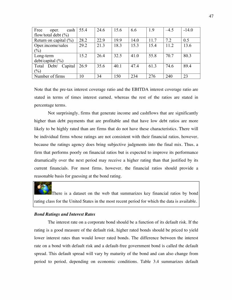
47

Free oper. cash flow/total debt (%)

55.4 24.6 15.6 6.6 1.9 –4.5 -14.0

Return on capital (%) 28.2 22.9 19.9 14.0 11.7 7.2 0.5 Oper.income/sales (%)

29.2 21.3 18.3 15.3 15.4 11.2 13.6

Long-term debt/capital (%)

15.2 26.4 32.5 41.0 55.8 70.7 80.3

Total Debt/ Capital (%)

26.9 35.6 40.1 47.4 61.3 74.6 89.4

Number of firms 10 34 150 234 276 240 23

Note that the pre-tax interest coverage ratio and the EBITDA interest coverage ratio are

stated in terms of times interest earned, whereas the rest of the ratios are stated in

percentage terms.

Not surprisingly, firms that generate income and cashflows that are significantly

higher than debt payments that are profitable and that have low debt ratios are more

likely to be highly rated than are firms that do not have these characteristics. There will

be individual firms whose ratings are not consistent with their financial ratios, however,

because the ratings agency does bring subjective judgments into the final mix. Thus, a

firm that performs poorly on financial ratios but is expected to improve its performance

dramatically over the next period may receive a higher rating than that justified by its

current financials. For most firms, however, the financial ratios should provide a

reasonable basis for guessing at the bond rating.

There is a dataset on the web that summarizes key financial ratios by bond

rating class for the United States in the most recent period for which the data is available.

Bond Ratings and Interest Rates

The interest rate on a corporate bond should be a function of its default risk. If the

rating is a good measure of the default risk, higher rated bonds should be priced to yield

lower interest rates than would lower rated bonds. The difference between the interest

rate on a bond with default risk and a default-free government bond is called the default

spread. This default spread will vary by maturity of the bond and can also change from

period to period, depending on economic conditions. Table 3.4 summarizes default

48

spreads in early 2009 for ten-year bonds in each ratings class (using S&P ratings) and the

market interest rates on these bonds, based upon a treasury bond rate of 3.5%.

Table 3.4: Default Spreads for Ratings Classes: Early 2009 Rating Default Spread Interest rate on bond AAA 1.25% 4.75% AA 1.75% 5.25% A+ 2.25% 5.75% A 2.50% 6.00% A- 3.00% 6.50% BBB 3.50% 7.00% BB 4.25% 7.75% B+ 5.00% 8.50% B 6.00% 9.50% B- 7.25% 10.75% CCC 8.50% 12.00% CC 10.00% 13.50% C 12.00% 15.50% D 15.00% 18.50%

Source: bondsonline.com

Table 3.4 provides default spreads at a point in time, but default spreads not only vary

across time but they can vary for bonds with the same rating but different maturities. For

the bonds with higher ratings, the default spread generally widen for the longer

maturities. For bonds with lower ratings, the spreads may decrease as we go to longer

maturities, reflecting the fact that near term default risk is greater than long term default

risk. Historically, default spreads for every ratings class have increased during recessions

and decreased during economic booms. In figure 3.10, we take a look at the evolution of

default spreads for different bond rating classes through 2008:

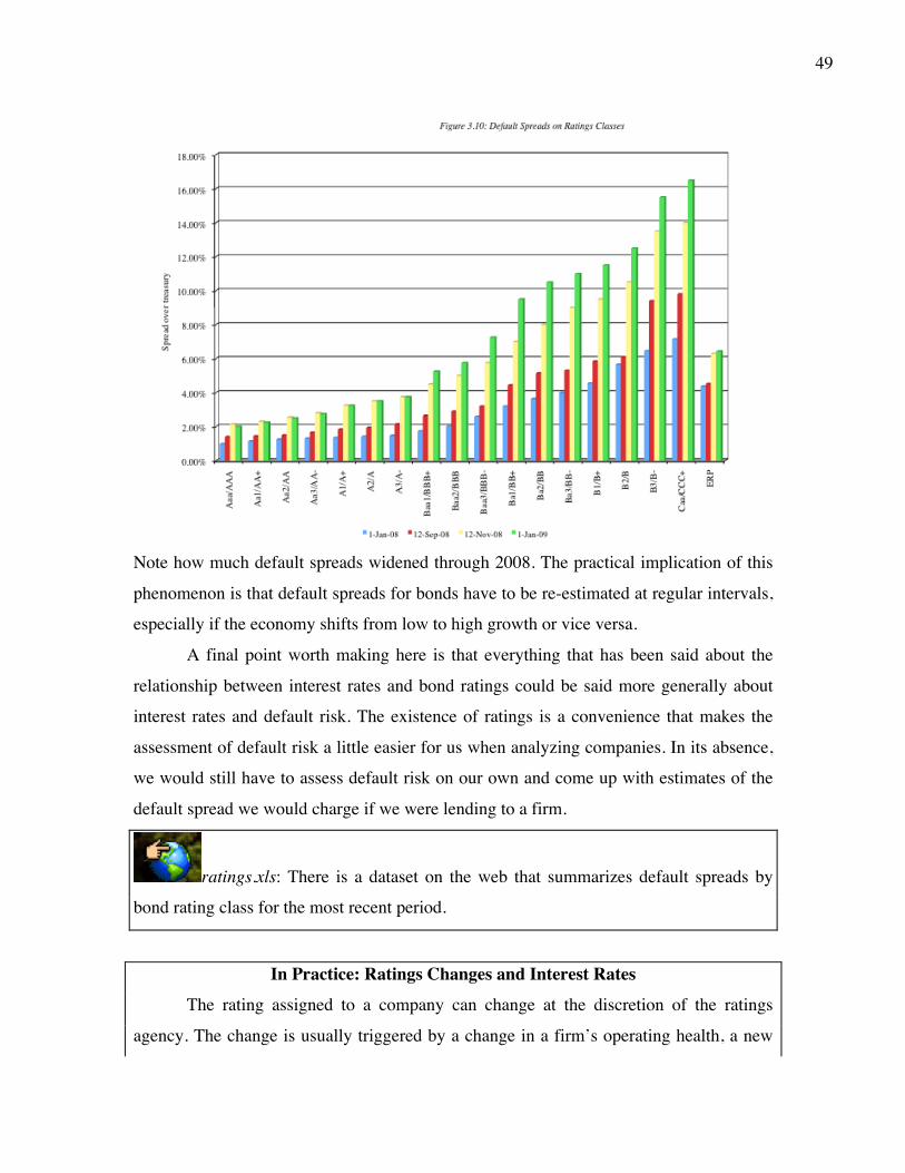
49

Note how much default spreads widened through 2008. The practical implication of this

phenomenon is that default spreads for bonds have to be re-estimated at regular intervals,

especially if the economy shifts from low to high growth or vice versa.

A final point worth making here is that everything that has been said about the

relationship between interest rates and bond ratings could be said more generally about

interest rates and default risk. The existence of ratings is a convenience that makes the

assessment of default risk a little easier for us when analyzing companies. In its absence,

we would still have to assess default risk on our own and come up with estimates of the

default spread we would charge if we were lending to a firm.

ratings.xls: There is a dataset on the web that summarizes default spreads by

bond rating class for the most recent period.

In Practice: Ratings Changes and Interest Rates The rating assigned to a company can change at the discretion of the ratings

agency. The change is usually triggered by a change in a firm’s operating health, a new

50

security issue by the firm or by new borrowing. Other things remaining equal, ratings will

drop if the operating performance deteriorates or if the firm borrows substantially more

and improve if it reports better earnings or if it raises new equity. In either case, though,

the ratings agency is reacting to news that the rest of the market also receives. In fact,

ratings agencies deliberate before making ratings changes, often putting a firm on a credit

watch list before changing its ratings. Since markets can react instantaneously, it should

come as no surprise that bond prices often decline before a ratings drop and increase

before a ratings increase. In fact, studies indicate that much of the bond price reaction to

deteriorating credit quality precedes a ratings drop.

This does not mean that there is no information in a ratings change. When ratings

are changed, the market still reacts but the reactions tend to be small. The biggest service

provided by ratings agencies may be in providing a measure of default risk that is

comparable across hundreds of rated firms, thus allowing bond investors a simple way of

categorizing their potential investments.

Conclusion Risk, as we define it in finance, is measured based upon deviations of actual

returns on an investment from its' expected returns. There are two types of risk. The first,

which we call equity risk, arises in investments where there are no promised cash flows,

but there are expected cash flows. The second,, default risk, arises on investments with

promised cash flows.

On investments with equity risk, the risk is best measured by looking at the

variance of actual returns around the expected returns, with greater variance indicating

greater risk. This risk can be broken down into risk that affects one or a few investments,

which we call firm specific risk, and risk that affects many investments, which we refer

to as market risk. When investors diversify, they can reduce their exposure to firm

specific risk. By assuming that the investors who trade at the margin are well diversified,

we conclude that the risk we should be looking at with equity investments is the market

risk. The different models of equity risk introduced in this chapter share this objective of

measuring market risk, but they differ in the way they do it. In the capital asset pricing

model, exposure to market risk is measured by a market beta, which estimates how much

51

risk an individual investment will add to a portfolio that includes all traded assets. The

arbitrage pricing model and the multi-factor model allow for multiple sources of market

risk and estimate betas for an investment relative to each source. Regression or proxy

models for risk look for firm characteristics, such as size, that have been correlated with

high returns in the past and use these to measure market risk. In all these models, the risk

measures are used to estimate the expected return on an equity investment. This expected

return can be considered the cost of equity for a company.

On investments with default risk, risk is measured by the likelihood that the

promised cash flows might not be delivered. Investments with higher default risk should

have higher interest rates, and the premium that we demand over a riskless rate is the

default premium. For most US companies, default risk is measured by rating agencies in

the form of a company rating; these ratings determine, in large part, the interest rates at

which these firms can borrow. Even in the absence of ratings, interest rates will include a

default premium that reflects the lenders’ assessments of default risk. These default-risk

adjusted interest rates represent the cost of borrowing or debt for a business.

52

Problems and Questions

1. The following table lists the stock prices for Microsoft from 1989 to 1998. The company did

not pay any dividends during the period Year Price 1989 $ 1.20 1990 $ 2.09 1991 $ 4.64 1992 $ 5.34 1993 $ 5.05 1994 $ 7.64 1995 $ 10.97 1996 $ 20.66 1997 $ 32.31 1998 $ 69.34

a. Estimate the average annual return you would have made on your investment

b. Estimate the standard deviation and variance in annual returns

c. If you were investing in Microsoft today, would you expect the historical standard

deviations and variances to continue to hold? Why or why not?

2. Unicom is a regulated utility serving Northern Illinois. The following table lists the stock

prices and dividends on Unicom from 1989 to 1998. Year Price Dividends 1989 $ 36.10 $ 3.00 1990 $ 33.60 $ 3.00 1991 $ 37.80 $ 3.00 1992 $ 30.90 $ 2.30 1993 $ 26.80 $ 1.60 1994 $ 24.80 $ 1.60 1995 $ 31.60 $ 1.60 1996 $ 28.50 $ 1.60 1997 $ 24.25 $ 1.60 1998 $ 35.60 $ 1.60

a. Estimate the average annual return you would have made on your investment

b. Estimate the standard deviation and variance in annual returns

c. If you were investing in Unicom today, would you expect the historical standard

deviations and variances to continue to hold? Why or why not?

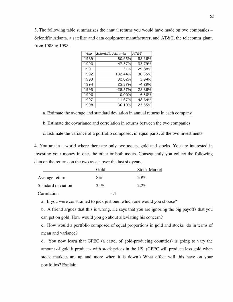
53

3. The following table summarizes the annual returns you would have made on two companies –

Scientific Atlanta, a satellite and data equipment manufacturer, and AT&T, the telecomm giant,

from 1988 to 1998. Year Scientific Atltanta AT&T 1989 80.95% 58.26% 1990 -47.37% -33.79% 1991 31% 29.88% 1992 132.44% 30.35% 1993 32.02% 2.94% 1994 25.37% -4.29% 1995 -28.57% 28.86% 1996 0.00% -6.36% 1997 11.67% 48.64% 1998 36.19% 23.55%

a. Estimate the average and standard deviation in annual returns in each company

b. Estimate the covariance and correlation in returns between the two companies

c. Estimate the variance of a portfolio composed, in equal parts, of the two investments

4. You are in a world where there are only two assets, gold and stocks. You are interested in

investing your money in one, the other or both assets. Consequently you collect the following

data on the returns on the two assets over the last six years.

Gold Stock Market

Average return 8% 20%

Standard deviation 25% 22%

Correlation -.4

a. If you were constrained to pick just one, which one would you choose?

b. A friend argues that this is wrong. He says that you are ignoring the big payoffs that you

can get on gold. How would you go about alleviating his concern?

c. How would a portfolio composed of equal proportions in gold and stocks do in terms of

mean and variance?

d. You now learn that GPEC (a cartel of gold-producing countries) is going to vary the

amount of gold it produces with stock prices in the US. (GPEC will produce less gold when

stock markets are up and more when it is down.) What effect will this have on your

portfolios? Explain.

54

5. You are interested in creating a portfolio of two stocks – Coca Cola and Texas Utilities. Over

the last decade, an investment in Coca Cola stock would have earned an average annual return of

25%, with a standard deviation in returns of 36%. An investment in Texas Utilities stock would

have earned an average annual return of 12%, with a standard deviation of 22%. The correlation

in returns across the two stocks is 0.28.

a. Assuming that the average and standard deviation, estimated using past returns, will

continue to hold in the future, estimate the average returns and standard deviation of a

portfolio composed 60% of Coca Cola and 40% of Texas Utilities stock.

b. Estimate the minimum variance portfolio.

c. Now assume that Coca Cola’s international diversification will reduce the correlation to

0.20, while increasing Coca Cola’s standard deviation in returns to 45%. Assuming all of

the other numbers remain unchanged, answer (a) and (b).

6. Assume that you have half your money invested in Times Mirror, the media company, and the

other half invested in Unilever, the consumer product giant. The expected returns and standard

deviations on the two investments are summarized below:

Times Mirror Unilever

Expected Return 14% 18%

Standard Deviation 25% 40%

Estimate the variance of the portfolio as a function of the correlation coefficient (Start with –1

and increase the correlation to +1 in 0.2 increments).

7. You have been asked to analyze the standard deviation of a portfolio composed of the

following three assets:

Investment Expected Return Standard Deviation

Sony Corporation 11% 23%

Tesoro Petroleum 9% 27%

Storage Technology 16% 50%

You have also been provided with the correlations across these three investments:

Sony Tesoro Storage Tech

Sony 1.00 -0.15 0.20

Tesoro -0.15 1.00 -0.25

55

Storage Tech 0.20 -0.25 1.00

Estimate the variance of a portfolio, equally weighted across all three assets.

8. You have been asked to estimate a Markowitz portfolio across a universe of 1250 assets.

a. How many expected returns and variances would you need to compute?

b. How many covariances would you need to compute to obtain Markowitz portfolios?

9. Assume that the average variance of return for an individual security is 50 and that the average

covariance is 10. What is the expected variance of a portfolio of 5, 10, 20, 50 and 100 securities.

How many securities need to be held before the risk of a portfolio is only 10% more than the

minimum?

10. Assume you have all your wealth (a million dollars) invested in the Vanguard 500 index

fund, and that you expect to earn an annual return of 12%, with a standard deviation in returns

of 25%. Since you have become more risk averse, you decide to shift $ 200,000 from the

Vanguard 500 index fund to treasury bills. The T.bill rate is 5%. Estimate the expected return

and standard deviation of your new portfolio.

11. Every investor in the capital asset pricing model owns a combination of the market portfolio

and a riskless asset. Assume that the standard deviation of the market portfolio is 30%, and that

the expected return on the portfolio is 15%. What proportion of the following investor’s wealth

would you suggest investing in the market portfolio and what proportion in the riskless asset?

(The riskless asset has an expected return of 5%)

a. an investor who desires a portfolio with no standard deviation

b. an investor who desires a portfolio with a standard deviation of 15%

c. an investor who desires a portfolio with a standard deviation of 30%

d. an investor who desires a portfolio with a standard deviation of 45%

e. an investor who desires a portfolio with an expected return of 12%

12. The following table lists returns on the market portfolio and on Microsoft, each year from

1989 to 1998. Year Microsoft Market Portfolio 1989 80.95% 31.49% 1990 -47.37% -3.17%

56

1991 31% 30.57% 1992 132.44% 7.58% 1993 32.02% 10.36% 1994 25.37% 2.55% 1995 -28.57% 37.57% 1996 0.00% 22.68% 1997 11.67% 33.10% 1998 36.19% 28.32%

a. Estimate the covariance in returns between Microsoft and the market portfolio

b. Estimate the variances in returns on both investments

c. Estimate the beta for Microsoft

13. United Airlines has a beta of 1.50. The standard deviation in the market portfolio is 22% and

United Airlines has a standard deviation of 66%

a. Estimate the correlation between United Airlines and the market portfolio.

b. What proportion of United Airlines’ risk is market risk?

14. You are using the arbitrage pricing model to estimate the expected return on Bethlehem

Steel, and have derived the following estimates for the factor betas and risk premia:

Factor Beta Risk Premia

1 1.2 2.5%

2 0.6 1.5%

3 1.5 1.0%

4 2.2 0.8%

5 0.5 1.2%

a. Which risk factor is Bethlehem Steel most exposed to? Is there any way, within the

arbitrage pricing model, to identify the risk factor?

b. If the riskfree rate is 5%, estimate the expected return on Bethlehem Steel

c. Now assume that the beta in the capital asset pricing model for Bethlehem Steel is 1.1,

and that the risk premium for the market portfolio is 5%. Estimate the expected return, using

the CAPM.

d. Why are the expected returns different using the two models?

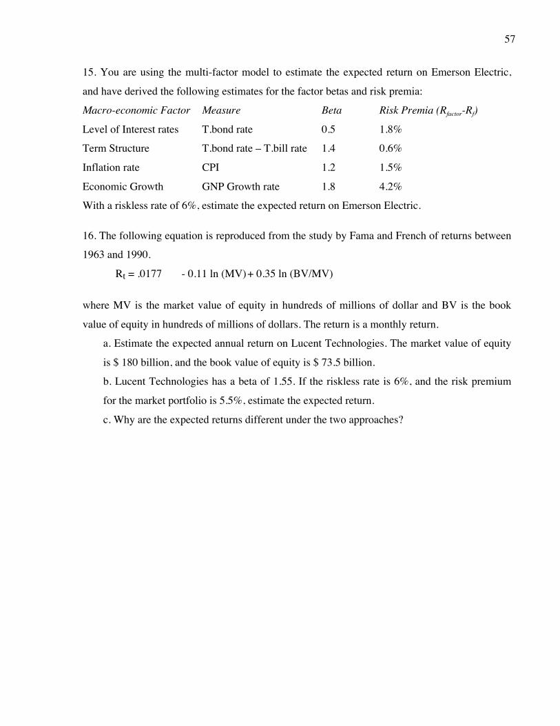
57

15. You are using the multi-factor model to estimate the expected return on Emerson Electric,

and have derived the following estimates for the factor betas and risk premia:

Macro-economic Factor Measure Beta Risk Premia (Rfactor-Rf)

Level of Interest rates T.bond rate 0.5 1.8%

Term Structure T.bond rate – T.bill rate 1.4 0.6%

Inflation rate CPI 1.2 1.5%

Economic Growth GNP Growth rate 1.8 4.2%

With a riskless rate of 6%, estimate the expected return on Emerson Electric.

16. The following equation is reproduced from the study by Fama and French of returns between

1963 and 1990.

Rt = .0177 - 0.11 ln (MV) + 0.35 ln (BV/MV)

where MV is the market value of equity in hundreds of millions of dollar and BV is the book

value of equity in hundreds of millions of dollars. The return is a monthly return.

a. Estimate the expected annual return on Lucent Technologies. The market value of equity

is $ 180 billion, and the book value of equity is $ 73.5 billion.

b. Lucent Technologies has a beta of 1.55. If the riskless rate is 6%, and the risk premium

for the market portfolio is 5.5%, estimate the expected return.

c. Why are the expected returns different under the two approaches?

58

Live Case Study

Stockholder Analysis Objective: To find out who the average and marginal investors in the company are. This

is relevant because risk and return models in finance assume that the marginal investor is

well diversified.

Key Questions:

• Who is the average investor in this stock? (Individual or pension fund, taxable or tax-

exempt, small or large, domestic or foreign)

• Who is the marginal investor in this stock?

Framework for Analysis

1. Who holds stock in this company?

• How many stockholders does the company have?

• What percent of the stock is held by institutional investors?

• Does the company have listings in foreign markets? (If you can, estimate the

percent of the stock held by non-domestic investors)

2. Insider Holdings

• Who are the insiders in this company? (Besides the managers and directors,

anyone with more than 5% is treated as an insider)

• What role do the insiders play in running the company?

• What percent of the stock is held by insiders in the company?

• What percent of the stock is held by employees overall? (Include the holdings

by employee pension plans)

• Have insiders been buying or selling stock in this company in the most recent

year?

Getting Information on Stockholder Composition

Information about insider and institutional ownership of firms is widely available

since both groups have to file with the SEC. These SIC filings are used to develop

rankings of the largest holders of stock in firms. Insider activity (buying and selling) is

59

also recorded by the SEC, though the information is not available until a few weeks after

the filing.

Online sources of information:

http://www.stern.nyu.edu/~adamodar/cfin2E/project/data.htm

4.1

1

CHAPTER 4

RISK MEASUREMENT AND HURDLE RATES IN PRACTICE

In the last chapter, we presented the argument that the expected return on an

equity investment should be a function of the market or non-diversifiable risk embedded

in that investment. Here we turn our attention to how best to estimate the parameters of

market risk in each of the models described in the previous chapter—the capital asset

pricing model, the arbitrage pricing model, and the multifactor model. We will present

three alternative approaches for measuring the market risk in an investment; the first is to

use historical data on market prices for the firm considering the project, the second is to

use the market risk parameters estimated for other firms that are in the same business as

the project being analyzed, and the third is to use accounting earnings or revenues to

estimate the parameters.

In addition to estimating market risk, we will also discuss how best to estimate a

riskless rate and a risk premium (in the CAPM) or risk premiums (in the APM and

multifactor models) to convert the risk measures into expected returns. We will present a

similar argument for bringing default risk into a cost of debt and then bring the discussion

to fruition by combining both the cost of equity and debt to estimate a cost of capital,

which will become the minimum acceptable hurdle rate for an investment.

Cost of Equity

The cost of equity is the rate of return that investors require to invest in the equity

of a firm. All of the risk and return models described in the previous chapter need a risk-

free rate and a risk premium (in the CAPM) or premiums (in the APM and multifactor

models). We begin by discussing those common inputs before turning attention to the

estimation of risk parameters.

I. Risk-Free Rate

Most risk and return models in finance start off with an asset that is defined as risk-

free and use the expected return on that asset as the risk-free rate. The expected returns

4.2

2

on risky investments are then measured relative to the risk-free rate, with the risk creating

an expected risk premium that is added on to the risk-free rate.

Requirements for an Asset to be Risk-Free

We defined a risk-free asset as one for which the investor knows the expected

returns with certainty. Consequently, for an investment to be risk-free, that is, to have an

actual return be equal to the expected return, two conditions have to be met:

• There has to be no default risk, which generally implies that the security has to be

issued by a government. Note, though, that not all governments are default-free, and

the presence of government or sovereign default risk can make it very difficult to

estimate risk-free rates in some currencies.

• There can be no uncertainty about reinvestment rates, which implies that there are no

intermediate cash flows. To illustrate this point, assume that you are trying to

estimate the expected return over a five-year period and that you want a risk-free rate.

A six-month Treasury bill rate, although default-free, will not be risk-free, because

there is the reinvestment risk of not knowing what the bill rate will be in six months.

Even a five-year Treasury bond is not risk-free, because the coupons on the bond will

be reinvested at rates that cannot be predicted today. The risk-free rate for a five-year

time horizon has to be the expected return on a default-free (government) five-year

zero coupon bond.

This clearly has painful implications for anyone doing corporate financial analysis, where

expected returns often have to be estimated for periods ranging over multiple years. A

purist’s view of risk-free rates would then require different risk-free rates for each period

and different expected returns. As a practical compromise, however, it is worth noting

that the present value effect of using risk-free rates that vary from year to year tends to be

small for most well-behaved term structures.1 In these cases, we could use a duration

matching strategy, where the duration of the default-free security used as the risk-free

asset is matched up to the duration of the cash flows in the analysis.2 If, however, there

1By “well-behaved term structures”, I would include a normal upwardly sloping yield curve, where long term rates are at most 2–3 percent higher than short-term rates. 2In investment analysis, where we look at projects, these durations are usually between three and ten years. In valuation, the durations tend to be much longer, because firms are assumed to have infinite lives. The

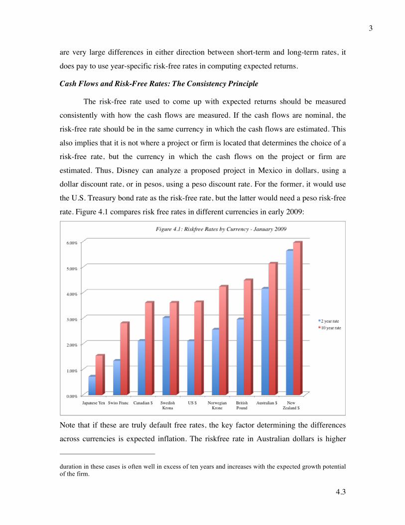
4.3

3

are very large differences in either direction between short-term and long-term rates, it

does pay to use year-specific risk-free rates in computing expected returns.

Cash Flows and Risk-Free Rates: The Consistency Principle

The risk-free rate used to come up with expected returns should be measured

consistently with how the cash flows are measured. If the cash flows are nominal, the

risk-free rate should be in the same currency in which the cash flows are estimated. This

also implies that it is not where a project or firm is located that determines the choice of a

risk-free rate, but the currency in which the cash flows on the project or firm are

estimated. Thus, Disney can analyze a proposed project in Mexico in dollars, using a

dollar discount rate, or in pesos, using a peso discount rate. For the former, it would use

the U.S. Treasury bond rate as the risk-free rate, but the latter would need a peso risk-free

rate. Figure 4.1 compares risk free rates in different currencies in early 2009:

Note that if these are truly default free rates, the key factor determining the differences

across currencies is expected inflation. The riskfree rate in Australian dollars is higher

duration in these cases is often well in excess of ten years and increases with the expected growth potential of the firm.

4.4

4

than the riskfre rate in Swiss Francs, because expected inflation is higher in Australia

than in Switzerland.

Under conditions of high and unstable inflation, valuation is often done in real

terms. Effectively, this means that cash flows are estimated using real growth rates and

without allowing for the growth that comes from price inflation. To be consistent, the

discount rates used in these cases have to be real discount rates. To get a real expected

rate of return, we need to start with a real risk-free rate. Although government bills and

bonds offer returns that are risk-free in nominal terms, they are not risk-free in real terms,

because inflation can be volatile. The standard approach of subtracting an expected

inflation rate from the nominal interest rate to arrive at a real risk-free rate provides at

best only an estimate of the real risk-free rate. Until recently, there were few traded

default-free securities that could be used to estimate real risk-free rates; but the

introduction of inflation-indexed Treasuries (called TIPs) has filled this void. An

inflation-indexed Treasury security does not offer a guaranteed nominal return to buyers,

but instead provides a guaranteed real return. In early 2008, for example, the inflation

indexed U.S. ten-year Treasury bond rate was only 1.4 percent, much lower than the

nominal ten-year bond rate of 3 percent.

4.1. What Is the Right Risk-Free Rate? The correct risk-free rate to use in the CAPM

a. is the short term government security rate.

b. is the long term government security rate.

c. can be either, depending on whether the prediction is short-term or long-term.

In Practice: What If There Is No Default-Free Rate?

Our discussion to this point has been predicated on the assumption that governments do

not default, at least on local borrowing. There are many emerging market economies

where this assumption might not be viewed as reasonable. Governments in these markets

are perceived as capable of defaulting even on local borrowing. When this is coupled

with the fact that many governments do not borrow long-term in the local currency, there

are scenarios in which obtaining a risk-free rate in that currency, especially for the long

4.5

5

term, becomes difficult. In these cases, there are compromises that give us reasonable

estimates of the risk-free rate.

• If the government does issue long-term bonds in the local currency, you could adjust

the government bond rate by the estimated default spread on the bond to arrive at a

riskless local currency rate. The default spread on the government bond can be

estimated using the local currency ratings that are available for many countries.3 In

May 2009, for instance, the ten-year rupee denominated Indian government bond rate

was 7%. However, the local currency sovereign rating assigned to the Indian

government in January 2009 by Moody’s was Ba2, indicating that they (Moody’s)

perceive default risk in Indian government rupee bonds. If the default spread for Ba2

rated government bonds is 3%, the rupee risk free is 4%.4

Rupee Riskfree Rate = Indian government bond rate – Default spread for India

= 7% - 3% = 4%

• If there are long-term dollar-denominated forward contracts on the currency, you can

use interest rate parity and the Treasury bond rate (or riskless rate in any other base

currency) to arrive at an estimate of the local borrowing rate. For instance, if the

current spot rate is 38.10 Thai baht per U.S. dollar, the ten-year forward rate is 61.36

baht per dollar and the current ten-year U.S. Treasury bond rate is 5 percent, the ten-

year Thai risk-free rate (in nominal baht) can be estimated as follows:

€

61.36 = 38.1( ) 1+ Interest RateThai Baht1+ 0.05

⎛

⎝ ⎜

⎞

⎠ ⎟ 10

Solving for the Thai interest rate yields a ten-year risk free rate of 10.12%.

If every attempt at estimating a riskfree rate in the local currency falls short, the fall back

position is to do your entire analysis in a different currency, where estimation poses

fewer challenges. Thus, we can analyze a Russian company in Euros or a Brazilian

company in U.S. dollars. If we do so, though, we have to be consistent and estimate all of

3Ratings agencies generally assign different ratings for local currency borrowings and dollar borrowings, with higher ratings for the former and lower ratings for the latter. 4 The default spread for a sovereign rating is computed by comparing dollar or euro denominated sovereign bonds issued by emerging markets to the default free US rate (treasury) or Euro rate (the German 10-year bond).

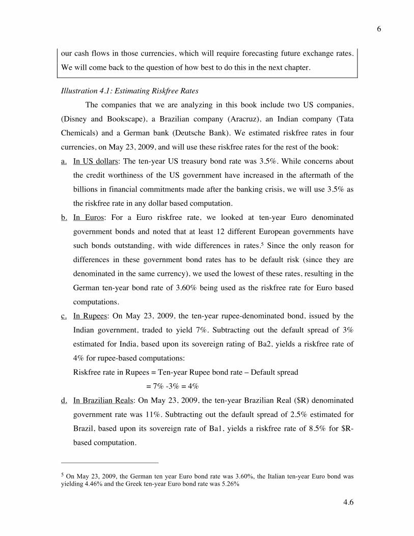
4.6

6

our cash flows in those currencies, which will require forecasting future exchange rates.

We will come back to the question of how best to do this in the next chapter.

Illustration 4.1: Estimating Riskfree Rates

The companies that we are analyzing in this book include two US companies,

(Disney and Bookscape), a Brazilian company (Aracruz), an Indian company (Tata

Chemicals) and a German bank (Deutsche Bank). We estimated riskfree rates in four

currencies, on May 23, 2009, and will use these riskfree rates for the rest of the book:

a. In US dollars: The ten-year US treasury bond rate was 3.5%. While concerns about

the credit worthiness of the US government have increased in the aftermath of the

billions in financial commitments made after the banking crisis, we will use 3.5% as

the riskfree rate in any dollar based computation.

b. In Euros: For a Euro riskfree rate, we looked at ten-year Euro denominated

government bonds and noted that at least 12 different European governments have

such bonds outstanding, with wide differences in rates.5 Since the only reason for

differences in these government bond rates has to be default risk (since they are

denominated in the same currency), we used the lowest of these rates, resulting in the

German ten-year bond rate of 3.60% being used as the riskfree rate for Euro based

computations.

c. In Rupees: On May 23, 2009, the ten-year rupee-denominated bond, issued by the

Indian government, traded to yield 7%. Subtracting out the default spread of 3%

estimated for India, based upon its sovereign rating of Ba2, yields a riskfree rate of

4% for rupee-based computations:

Riskfree rate in Rupees = Ten-year Rupee bond rate – Default spread

= 7% -3% = 4%

d. In Brazilian Reals: On May 23, 2009, the ten-year Brazilian Real ($R) denominated

government rate was 11%. Subtracting out the default spread of 2.5% estimated for

Brazil, based upon its sovereign rate of Ba1, yields a riskfree rate of 8.5% for $R-

based computation.

5 On May 23, 2009, the German ten year Euro bond rate was 3.60%, the Italian ten-year Euro bond was yielding 4.46% and the Greek ten-year Euro bond rate was 5.26%

4.7

7

e. In real terms: For any computations done in real terms, we need a real riskfree rate.

We will use the ten-year inflation-indexed treasury bond (TIPS) rate of 1.6% (from

May 23, 2009) as the riskfree rate for any computations done in real terms.

II. Risk Premium The risk premium(s) is clearly a significant input in all of the asset pricing

models. In the following section, we will begin by examining the fundamental

determinants of risk premiums and then look at practical approaches to estimating these

premiums.

What Is the Risk Premium Supposed to Measure?

The risk premium in the CAPM measures the extra return that would be

demanded by investors for shifting their money from a riskless investment to the market

portfolio or risky investments, on average. It should be a function of two variables:

1. Risk Aversion of Investors: As investors become more risk-averse, they should

demand a larger premium for shifting from the riskless asset. Although some of this

risk aversion may be inherent, some of it is also a function of economic prosperity

(when the economy is doing well, investors tend to be much more willing to take risk)

and recent experiences in the market (risk premiums tend to surge after large market

drops).

2. Riskiness of the Average Risk Investment: As the riskiness of the average risk

investment increases, so should the premium. This will depend on what firms are

actually traded in the market, their economic fundamentals, and how involved they

are in managing risk.

Because each investor in a market is likely to have a different assessment of an

acceptable equity risk premium, the premium will be a weighted average of these

individual premiums, where the weights will be based on the wealth the investor brings to

the market. Put more directly, what Warren Buffett, with his substantial wealth, thinks is

an acceptable premium will be weighted in far more into market prices than what you or I

might think about the same measure.

4.8

8

In the APM and the multifactor models, the risk premiums used for individual

factors are similar wealth-weighted averages of the premiums that individual investors

would demand for each factor separately.

4.2 What Is Your Risk Premium? Assume that stocks are the only risky assets and that you are offered two investment

options:

• A riskless investment (say, a government security), on which you can make 4 percent

• A mutual fund of all stocks, on which the returns are uncertain

How much of an expected return would you demand to shift your money from the

riskless asset to the mutual fund?

a. Less than 4 percent

b. Between 4 and 6 percent

c. Between 6 and 8 percent

d. Between 8 and10 percent

e. Between 10 and 12 percent

f. More than 12 percent

Your answer to this question should provide you with a measure of your risk premium.

(For instance, if your answer is 6 percent, your premium is 2 percent.)

Estimating Risk Premiums

There are three ways of estimating the risk premium in the CAPM: Large

investors can be surveyed about their expectations for the future, the actual premiums

earned over a past period can be obtained from historical data, and the implied premium

can be extracted from current market data. The premium can be estimated only from

historical data in the APM and the multi-factor models.

1. Survey Premiums

Because the premium is a weighted average of the premiums demanded by

individual investors, one approach to estimating this premium is to survey investors about

their expectations for the future. It is clearly impractical to survey all investors; therefore,

most surveys focus on portfolio managers or Chief Financial Officers (CFOs), who carry

4.9

9

the most weight in the process. Table 4.1 summarizes the results of some of these

surveys, along with the groups surveyed:

Table 4.1: Equity Risk Premiums from Surveys

Group Surveyed Survey done by Results (Year) Individual Investors Securities Industry Association 8.3% (December 2004) Institutional Investors Merrill Lynch 3.8% (July 2008) CFOs Campbell and Harvey 4.2% (March 2008) Finance academics Fernandez 6.2% (2008)

Although numbers do emerge from these surveys, very few practitioners actually use

these survey premiums. There are three reasons for this reticence:

• There are no constraints on reasonability; individual money managers could provide

expected returns that are lower than the risk-free rate, for instance.

• Survey premiums are extremely volatile; the survey premiums can change

dramatically, largely as a function of recent market movements.

• Survey premiums tend to be short-term; even the longest surveys do not go beyond

one year.

4.3 Do Risk Premiums Change? In the previous question, you were asked how much of a premium you would demand for

investing in a portfolio of stocks as opposed to a riskless asset. Assume that the market

dropped by 20 percent last week, and you were asked the same question today. Would

your premium be

a. higher?

b. lower?

c. unchanged?

2. Historical Premiums

The most common approach to estimating the risk premium(s) used in financial

asset pricing models is to base it on historical data. In the APM and multifactor models,

the premiums are based on historical data on asset prices over very long time periods

which are used to extract factor-specific risk premiums. In the CAPM, the premium is

defined as the difference between average returns on stocks and average returns on risk-

free securities over an extended period of history.

4.10

10

Basics

In most cases, this approach is composed of the following steps. It begins by

defining a time period for the estimation, which can range to as far back as 1871 for U.S.

data. It then requires the calculation of the average returns on a stock index and average

returns on a riskless security over the period. Finally, the difference between the average

returns on stocks and the riskless return it is defined as the risk premium looking

forward. In doing this, we implicitly assume that

1. The risk aversion of investors has not changed in a systematic way across

time. (The risk aversion may change from year to year, but it reverts back to

historical averages.)

2. The average riskiness of the “risky” portfolio (stock index) has not changed in

a systematic way across time.

Estimation Issues

Users of risk and return models may have developed a consensus that the historical

premium is in fact the best estimate of the risk premium looking forward, but there are

surprisingly large differences in the actual premiums used in practice. For instance, the

risk premium estimated in the U.S. markets by different investment banks, consultants,

and corporations range from 4 percent at the lower end to 12 percent at the upper end.

Given that they almost all use the same database of historical returns, provided by

Ibbotson Associates,6 summarizing data from 1926, these differences may seem

surprising. There are, however, three reasons for the divergence in risk premiums.

• Time Period Used: Although there are some who use all of the Ibbotson which goes

back to 1926, there are many using data over shorter time periods, such as fifty,

twenty, or even ten years to come up with historical risk premiums. The rationale

presented by those who use shorter periods is that the risk aversion of the average

investor is likely to change over time and using a shorter and more recent time period

provides a more updated estimate. This has to be offset against a cost associated with

using shorter time periods, which is the greater estimation error in the risk premium

4.11

11

estimate. In fact, given the annual standard deviation in stock prices between 1928

and 2008 of 20 percent,7 the standard error associated with the risk premium estimate

can be estimated as follows for different estimation periods in Table 4.2.8

Table 4.2 Standard Errors in Risk Premium Estimates

Estimation Period Standard Error of Risk Premium Estimate

5 years 20/√5 = 8.94%

10 years 20/√10 = 6.32%

25 years 20/√25 = 4.00%

50 years 20/√50 = 2.83%

Note that to get reasonable standard errors, we need very long time periods of

historical returns. Conversely, the standard errors from ten- and twenty-year estimates

are likely to be almost as large or larger than the actual risk premiums estimated. This

cost of using shorter time periods seems, in our view, to overwhelm any advantages

associated with getting a more updated premium.

• Choice of Risk-Free Security: The Ibbotson database reports returns on both Treasury

bills and bonds and the risk premium for stocks can be estimated relative to each.

Given that short term rates have been lower than long term rates in the United States

for most of the past seven decades, the risk premium is larger when estimated relative

to shorter-term government securities (such as Treasury bills). The risk-free rate

chosen in computing the premium has to be consistent with the risk-free rate used to

compute expected returns. For the most part, in corporate finance and valuation, the

risk-free rate will be a long-term government bond rate and not a short term rate.

Thus the risk premium used should be the premium earned by stocks over Treasury

bonds.

6See “Stocks, Bonds, Bills and Inflation,” an annual publication that reports on the annual returns on stocks, Treasury bonds and bills, and inflation rates from 1926 to the present. Available online at www.ibbotson.com. 7For the historical data on stock returns, bond returns, and bill returns, check under Updated Data at www.damodaran.com.. 8These estimates of the standard error are probably understated because they are based on the assumption that annual returns are uncorrelated over time. There is substantial empirical evidence that returns are correlated over time, which would make this standard error estimate much larger.

4.12

12

• Arithmetic and Geometric Averages: The final sticking point when it comes to

estimating historical premiums relates to how the average returns on stocks and

Treasury bonds and bills are computed. The arithmetic average return measures the

simple mean of the series of annual returns, whereas the geometric average looks at

the compounded return.9 Conventional wisdom argues for the use of the arithmetic

average. In fact, if annual returns are uncorrelated over time and our objective was to

estimate the risk premium for the next year, the arithmetic average is the best

unbiased estimate of the premium. In reality, however, there are strong arguments

that can be made for the use of geometric averages. First, empirical studies seem to

indicate that returns on stocks are negatively correlated over time.10 Consequently,

the arithmetic average return is likely to overstate the premium. Second, although

asset pricing models may be single-period models, the use of these models to get

expected returns over long periods (such as five or ten years) suggests that the

analysis is more likely to be over multiple years than for just the next year. In this

context, the argument for geometric average premiums becomes even stronger. In summary, the risk premium estimates vary across users because of differences in time

periods used, the choice of Treasury bills or bonds as the risk-free rate, and the use of

arithmetic as opposed to geometric averages. The effect of these choices is summarized

in Table 4.3, which uses returns from 1928 to 2008.11

Table 4.3 Historical Risk Premiums (%) for the United States, 1928- 2008

Stocks – Treasury Bills Stocks – Treasury Bonds Arithmetic Geometric Arithmetic Geometric

1928–2008 7.30% 5.65% 5.32% 3.88%

9The compounded return is computed by taking the value of the investment at the start of the period (Value0) and the value at the end (ValueN) and then computing the following:

Geometric Average = Value NValue0

⎛

⎝ ⎜

⎞

⎠ ⎟

1/ N

− 1

10In other words, good years are more likely to be followed by poor years and vice versa. The evidence on negative serial correlation in stock returns over time is extensive and can be found in Fama, E.F. and K.R. French, 1988, Permanent and Temporary Components of Stock Prices, Journal of Political Economy, v96, 246-273. Although they find that the one-year correlations are low, the five-year serial correlations are strongly negative for all size classes. 11The raw data on Treasury bill rates, Treasury bond rates, and stock returns was obtained from the Federal Reserve data archives maintained by the Fed in St. Louis.

4.13

13

1959–2008 5.14% 3.33% 3.77% 2.29% 1999–2008 -2.53% -6.26% -4.53% -7.96%

Note that the premiums range from negative values (for the ten-year premiums) to values

as high as 7.30% (which is the arithmetic average of the premium over treasury bills), If

we follow the propositions about picking a long-term geometric average premium over

the long-term Treasury bond rate, the historical risk premium that makes the most sense

is 3.88 percent.

Historical Premiums in Other Markets

Although historical data on stock returns is easily available and accessible in the

United States, it is much more difficult to get for foreign markets. The most detailed look

at these returns estimated the returns you would have earned on fourteen equity markets

between 1900 and 2005 and compared these returns with those you would have earned

investing in bonds.12 Table 4.4 presents the risk premiums—that is, the additional

returns—earned by investing in equity over short term and long term government bonds

over that period in each of the fourteen markets.

Table 4.4 Equity Risk Premiums by Country

Stocks minus Short term Governments Stocks minus Long term Governments

Country Geometric

Mean Arithmetic

Mean Standard

Error Standard Deviation

Geometric Mean

Arithmetic Mean

Standard Error

Standard Deviation

Australia 7.08 8.49 1.65 17.00 6.22 7.81 1.83 18.80 Belgium 2.80 4.99 2.24 23.06 2.57 4.37 1.95 20.10 Canada 4.54 5.88 1.62 16.71 4.15 5.67 1.74 17.95 Denmark 2.87 4.51 1.93 19.85 2.07 3.27 1.57 16.18 France 6.79 9.27 2.35 24.19 3.86 6.03 2.16 22.29 Germany* 3.83 9.07 3.28 33.49 5.28 8.35 2.69 27.41 Ireland 4.09 5.98 1.97 20.33 3.62 5.18 1.78 18.37 Italy 6.55 10.46 3.12 32.09 4.30 7.68 2.89 29.73 Japan 6.67 9.84 2.70 27.82 5.91 9.98 3.21 33.06 Netherlands 4.55 6.61 2.17 22.36 3.86 5.95 2.10 21.63 Norway 3.07 5.70 2.52 25.90 2.55 5.26 2.66 27.43 South Africa 6.20 8.25 2.15 22.09 5.35 7.03 1.88 19.32 Spain 3.40 5.46 2.08 21.45 2.32 4.21 1.96 20.20

12Dimson, E.,, P Marsh and M Staunton, 2002, Triumph of the Optimists: 101 Years of Global Investment Returns, Princeton University Press, NJ and Global Investment Returns Yearbook, 2006, ABN AMRO/London Business School.

4.14

14

Sweden 5.73 7.98 2.15 22.09 5.21 7.51 2.17 22.34 Switzerland 3.63 5.29 1.82 18.79 1.80 3.28 1.70 17.52 U.K. 4.43 6.14 1.93 19.84 4.06 5.29 1.61 16.60 U.S. 5.51 7.41 1.91 19.64 4.52 6.49 1.96 20.16 World-ex U.S. 4.23 5.93 1.88 19.33 4.10 5.18 1.48 15.19 World 4.74 6.07 1.62 16.65 4.04 5.15 1.45 14.96 The differences in compounded annual returns between stocks and short-term governments/long-term governments is reported for each country..

Although equity returns were higher than what you would have earned investing in

government bonds or bills in each of the countries examined, there are wide differences

across countries. If you had invested in Spain, for instance, you would have earned only 3

percent over government bills and 2.3 percent over government bonds on an annual basis

by investing in equities. In France, in contrast, the corresponding numbers would have

been 6.8 percent and 3.9 percent. When looking at forty or fifty-year periods, therefore, it

is entirely possible that equity returns can lag bond or bill returns, at least in some equity

markets. In other words, the notion that stocks always win in the long run is not only

dangerous but does not make sense. If stocks always beat riskless investments in the long

run, they should be riskless to an investor with a long time horizon.

histretSP.xls: This data set has yearly data on Treasury bill rates, Treasury bond

rates, and returns and stock returns going back to 1928.

A Modified Historical Risk Premium

In many emerging markets, there is very little historical data, and what does exist

is too volatile to yield a meaningful estimate of the risk premium. To estimate the risk

premium in these countries, let us start with the basic proposition that the risk premium in

any equity market can be written as

Equity Risk Premium = Base Premium for Mature Equity Market + Country Premium

The country premium could reflect the extra risk in a specific market. This boils down

our estimation to answering two questions:

• What should the base premium for a mature equity market be?

• How do we estimate the additional risk premium for individual countries?

To answer the first question, we will make the argument that the U.S. equity market is

mature and that there is sufficient historical data to make a reasonable estimate of the risk

4.15

15

premium. In fact, reverting back to our discussion of historical premiums in the U.S.

market, we will use the geometric average premium earned by stocks over Treasury

bonds of 3.88 percent between 1928 and 2008. We chose the long time period to reduce

the standard error in our estimate, the Treasury bond to be consistent with our choice of a

risk-free rate, and geometric averages to reflect our desire for a risk premium that we can

use for longer-term expected returns. There are three approaches that we can use to

estimate the country risk premium.

1. Country Bond Default Spreads: There are several measures of country risk, and one

of the simplest and most easily accessible is the rating assigned to a country’s debt by

a ratings agency (S&P, Moody’s, and IBCA all rate countries). These sovereign

ratings measure default risk (rather than equity risk), but they are affected by many of

the factors that drive equity risk—the stability of a country’s currency, its budget and

trade balances, and its political stability, for instance.13 The other advantage of ratings

is that they come with default spreads over the U.S. Treasury bond. To illustrate, in

May 2009, Moody’s assigned ratings of Ba1 to Brazil and Ba2 to India; the typical

default spread at the time was 2.5% for a Ba1 rated sovereign bond and 3% for a Ba2

rated sovereign bond.14

Analysts who use default spreads as measures of country risk typically add them

on to both the cost of equity and debt of every company traded in that country. For

instance, the cost of equity for a Brazilian company, estimated in U.S. dollars, will be

2.5 percent higher than the cost of equity of an otherwise similar U.S. company. If we

assume that the risk premium for the United States and other mature equity markets is

3.88 percent, the cost of equity for a Brazilian company with a beta of 1.2 can be

estimated as follows (with a U.S. Treasury bond rate of 3.5 percent).

Cost of equity = Risk-free rate + Beta * (U.S. Risk premium) + Country Bond Default

Spread

= 3.5% + 1.2(3.88%) + 2.50% = 10.65%

13The process by which country ratings are obtained is explained on the S&P Web site at www.ratings.standardpoor.com/criteria/index.htm. 14 We estimated these spreads by looking at dollar or euro denominated bonds issued by governments with these ratings and comparing the rates on these bonds to the US treasury (for dollar bonds) and the German Euro bond (for Euro bonds).

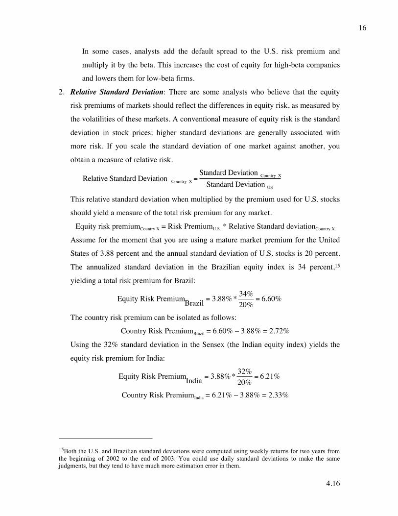
4.16

16

In some cases, analysts add the default spread to the U.S. risk premium and

multiply it by the beta. This increases the cost of equity for high-beta companies

and lowers them for low-beta firms.

2. Relative Standard Deviation: There are some analysts who believe that the equity

risk premiums of markets should reflect the differences in equity risk, as measured by

the volatilities of these markets. A conventional measure of equity risk is the standard

deviation in stock prices; higher standard deviations are generally associated with

more risk. If you scale the standard deviation of one market against another, you

obtain a measure of relative risk.

€

Relative Standard Deviation Country X =Standard Deviation Country X

Standard Deviation US

This relative standard deviation when multiplied by the premium used for U.S. stocks

should yield a measure of the total risk premium for any market.

Equity risk premiumCountry X = Risk PremiumU.S. * Relative Standard deviationCountry X

Assume for the moment that you are using a mature market premium for the United

States of 3.88 percent and the annual standard deviation of U.S. stocks is 20 percent.

The annualized standard deviation in the Brazilian equity index is 34 percent,15

yielding a total risk premium for Brazil:

€

Equity Risk PremiumBrazil = 3.88% * 34%20%

= 6.60%

The country risk premium can be isolated as follows:

Country Risk PremiumBrazil = 6.60% – 3.88% = 2.72%

Using the 32% standard deviation in the Sensex (the Indian equity index) yields the

equity risk premium for India:

€

Equity Risk PremiumIndia = 3.88% * 32%20%

= 6.21%

Country Risk PremiumIndia = 6.21% – 3.88% = 2.33%

15Both the U.S. and Brazilian standard deviations were computed using weekly returns for two years from the beginning of 2002 to the end of 2003. You could use daily standard deviations to make the same judgments, but they tend to have much more estimation error in them.

4.17

17

Although this approach has intuitive appeal, there are problems with using standard

deviations computed in markets with widely different market structures and liquidity.

There are very risky emerging markets that have low standard deviations for their

equity markets because the markets are illiquid. This approach will understate the

equity risk premiums in those markets.

3. Default Spreads + Relative Standard Deviations: The country default spreads that

come with country ratings provide an important first step, but still only measure the

premium for default risk. Intuitively, we would expect the country equity risk

premium to be larger than the country default risk spread since equities are riskier

than bonds. To address the issue of how much higher, we look at the volatility of the

equity market in a country relative to the volatility of the country bond used to

estimate the default spread. This yields the following estimate for the country equity

risk premium.

€

Country Risk Premium = Country Default Spread *σEquity

σ Country Bond

⎛

⎝ ⎜

⎞

⎠ ⎟

To illustrate, consider the case of Brazil. As noted earlier, the dollar-denominated

bonds issued by the Brazilian government trade with a default spread of 3 percent

over the U.S. Treasury bond rate. The annualized standard deviation in the Brazilian

equity index over the previous year is 34.0 percent, whereas the annualized standard

deviation in the Brazilian C-bond is 21.5 percent.16 The resulting additional country

equity risk premium for Brazil is as follows:

€

Brazil's Country Risk Premium = 2.50% 34.0%21.5%⎛

⎝ ⎜

⎞

⎠ ⎟ = 3.95%

Note that this country risk premium will increase if the country default spread widens

or if the relative volatility of the equity market increases. It is also in addition to the

equity risk premium for a mature market. Thus the total equity risk premium for a

Brazilian company using the approach and a 3.88 percent premium for the United

16The standard deviation in C-bond returns was computed using weekly returns over two years as well. Because these returns are in dollars and the returns on the Brazilian equity index are in real, there is an inconsistency here. We did estimate the standard deviation on the Brazilian equity index in dollars, but it

4.18

18

States would be 7.63 percent. Using the same approach for India, where the Indian

government bond had a standard deviation of 21.3% yield the country risk premium

for India:

€

India's Country Risk Premium = 3.00% 32.0%21.3%⎛

⎝ ⎜

⎞

⎠ ⎟ = 4.51%

Total Equity Risk PremiumIndia = 3.88% + 4.51% = 8.39%

Why should equity risk premiums have any relationship to country bond default

spreads? A simple explanation is that an investor who can make 6 percent on a dollar-

denominated Brazilian government bond would not settle for an expected return of

5.5 percent (in dollar terms) on Brazilian equity. This approach and the previous one

both use the standard deviation in equity of a market to make a judgment about

country risk premium, but they measure it relative to different bases. This approach

uses the country bond as a base, whereas the previous one uses the standard deviation

in the U.S. market. This approach assumes that investors are more likely to choose

between Brazilian government bonds and Brazilian equity, whereas the previous

approach assumes that the choice is across equity markets.

The three approaches to estimating country risk premiums will generally give

different estimates, with the bond default spread and relative equity standard deviation

approaches yielding lower country risk premiums than the melded approach that uses

both the country bond default spread and the equity and bond market standard deviations.

Table 4.5 summarizes these estimates:

Table 4.5: Country Risk Premiums Estimates for India and Brazil – March 2009

Sovereign Rating

Default Spread

Relative Equity Market volatility

Composite Country risk premium

Brazil Ba1 2.50%

€

34%20%

(3.88%) − 3.88% = 2.72%

€

34%21.5%

(2.5%) = 3.95%

India Ba2 3.00%

€

32%20%

(3.88%) − 3.88% = 2.33%

€

32%21.3%

(3%) = 4.51%

We believe that the larger country risk premiums that emerge from the last

approach are the most realistic for the immediate future, but country risk premiums may

made little difference to the overall calculation because the dollar standard deviation was close to 36 percent.

4.19

19

decline over time. Just as companies mature and become less risky over time, countries

can mature and become less risky as well.

In Practice: Should There Be a Country Risk Premium?

Is there more risk in investing in a Malaysian or Brazilian stock than there is in

investing in the United States? The answer, to most, seems to be obviously affirmative.

That, however, does not answer the question of whether there should be an additional risk

premium charged when investing in those markets. Note that the only risk relevant for the

purpose of estimating a cost of equity is market risk or risk that cannot be diversified

away. The key question then becomes whether the risk in an emerging market is

diversifiable or non-diversifiable risk. If, in fact, the additional risk of investing in

Malaysia or Brazil can be diversified away, then there should be no additional risk

premium charged. If it cannot, then it makes sense to think about estimating a country

risk premium.

For purposes of analyzing country risk, we look at the marginal investor—the

investor most likely to be trading on the equity. If that marginal investor is globally

diversified, there is at least the potential for global diversification. If the marginal

investor does not have a global portfolio, the likelihood of diversifying away country risk

declines substantially. Even if the marginal investor is globally diversified, there is a

second test that has to be met for country risk to not matter. All or much of country risk

should be country-specific. In other words, there should be low correlation across

markets. Only then will the risk be diversifiable in a globally diversified portfolio. If, on

the other hand, stock markets across countries move together, country risk has a market

risk component, is not diversifiable, and should command a premium. Whether returns

across countries are positively correlated is an empirical question. Studies from the 1970s

and 1980s suggested that the correlation was low, and this was an impetus for global

diversification. Partly because of the success of that sales pitch and partly because

economies around the world have become increasingly intertwined over the past decade

or so, more recent studies indicate that the correlation across markets has risen. This is

borne out by the speed at which troubles in one market, say, Russia, can spread to a

market with which it has little or no obvious relationship, say, Brazil.

4.20

20

So where do we stand? We believe that although the barriers to trading across

markets have dropped, investors still have a home bias in their portfolios and that markets

remain partially segmented. Globally diversified investors are playing an increasing role

in the pricing of equities around the world, but the resulting increase in correlation across

markets has resulted in a portion of country risk becoming non-diversifiable or market

risk.

ctryprem.xls: There is a data set online that contains the updated ratings for

countries and the risk premiums associated with each.

3. Implied Equity Premiums

There is an alternative to estimating risk premiums that does not require historical

data or adjustments for country risk but does assume that the overall stock market is

correctly priced. Consider, for instance, a very simple valuation model for stocks

Value =

€

Expected Dividends Next Period(Required Return on Equity - Expected Growth Rate in Dividends)

This is essentially the present value of dividends growing at a constant rate. Three of the

four variables in this model can be obtained easily—the current level of the market (i.e.,

value), the expected dividends next period, and the expected growth rate in earnings and

dividends in the long term. The only unknown is then the required return on equity; when

we solve for it, we get an implied expected return on stocks. Subtracting out the risk-free

rate will yield an implied equity risk premium.

To illustrate, assume that the current level of the S&P 500 Index is 900, the

expected dividend yield on the index for the next period is 2 percent, and the expected

growth rate in earnings and dividends in the long run is 7 percent. Solving for the

required return on equity yields the following:

( ) 0.07-

02.0900900r

=

Solving for r,

r – 0.07 = 0.02

r = 0.09 = 9%

4.21

21

If the current risk-free rate is 6 percent, this will yield a premium of 3 percent.

This approach can be generalized to allow for high growth for a period and

extended to cover cash flow–based rather than dividend–based, models. To illustrate this,

consider the S&P 500 Index on January 1, 2009. On December 31, 2008, the S&P 500

Index closed at 903.25, and the dividend yield on the index was roughly 3.12%. In

addition, the consensus estimate of growth in earnings for companies in the index was

approximately 4% for the next 5 years.17 Since the companies in the index have bought

back substantial amounts of their own stock over the last few years, we considered

buybacks as part of the cash flows to equity investors. Table 4.6 summarizes dividends

and stock buybacks on the index, going back to 2001.

Table 4.6: Dividends and Stock Buybacks on S&P 500 Index: 2001-2008

Year

Market value of

index Dividends Buybacks

Cash to

equity Dividend

yield Buyback

yield Total yield

2001 1148.09 15.74 14.34 30.08 1.37% 1.25% 2.62% 2002 879.82 15.96 13.87 29.83 1.81% 1.58% 3.39% 2003 1111.91 17.88 13.70 31.58 1.61% 1.23% 2.84% 2004 1211.92 19.01 21.59 40.60 1.57% 1.78% 3.35% 2005 1248.29 22.34 38.82 61.17 1.79% 3.11% 4.90% 2006 1418.30 25.04 48.12 73.16 1.77% 3.39% 5.16% 2007 1468.36 28.14 67.22 95.36 1.92% 4.58% 6.49% 2008 903.25 28.47 40.25 68.72 3.15% 4.61% 7.77%

Normalized 903.25 28.47 24.11 52.584 3.15% 2.67% 5.82%

In 2008, for instance, firms collectively returned 7.77% of the index in the form of

dividends (3.15%) and stock buybacks (4.61%). Buybacks are volatile, and dropped

about 40% in the last quarter of 2008, relative to the last quarter of 2007, in the face of a

market crisis and a slowing economy. Since this slowdown is likely to continue into

2009, we reduced the buybacks in 2008 by 40% to compute a normalized cash yield of

5.82% for the year (resulting in a total cash to equity of 52.584 for the year). In table 4.7,

we estimate the cash flows to investors in the S&P 500 index from 2009-2014 by

growing the normalized cash flow at 4% a year for the first five years and 2.21% (set

equal to the riskfree rate) thereafter.

17 We used the average of the analyst estimates for individual firms (bottom-up). Alternatively, we could have used the top-down estimate for the S&P 500 earnings.

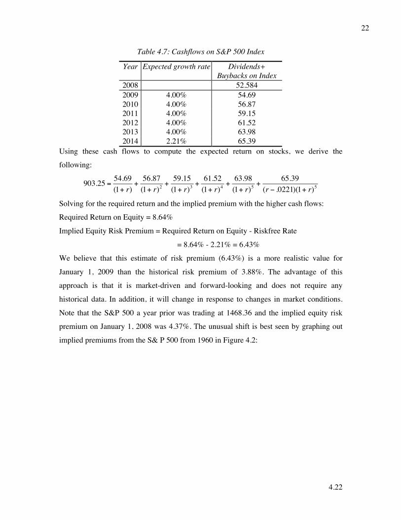
4.22

22

Table 4.7: Cashflows on S&P 500 Index

Year Expected growth rate Dividends+ Buybacks on Index

2008 52.584 2009 4.00% 54.69 2010 4.00% 56.87 2011 4.00% 59.15 2012 4.00% 61.52 2013 4.00% 63.98 2014 2.21% 65.39

Using these cash flows to compute the expected return on stocks, we derive the

following:

€

903.25 =54.69(1+ r)

+56.87(1+ r)2

+59.15(1+ r)3

+61.52(1+ r)4

+63.98(1+ r)5

+65.39

(r − .0221)(1+ r)5

Solving for the required return and the implied premium with the higher cash flows:

Required Return on Equity = 8.64%

Implied Equity Risk Premium = Required Return on Equity - Riskfree Rate

= 8.64% - 2.21% = 6.43%

We believe that this estimate of risk premium (6.43%) is a more realistic value for

January 1, 2009 than the historical risk premium of 3.88%. The advantage of this

approach is that it is market-driven and forward-looking and does not require any

historical data. In addition, it will change in response to changes in market conditions.

Note that the S&P 500 a year prior was trading at 1468.36 and the implied equity risk

premium on January 1, 2008 was 4.37%. The unusual shift is best seen by graphing out

implied premiums from the S& P 500 from 1960 in Figure 4.2:

4.23

23

In terms of mechanics, we used analyst estimates of growth rates in earnings and

dividends as our projected growth rates and a two-stage dividend discount model (similar

to the one that we used to compute the implied premium in the last paragraph). Looking

at these numbers, we would draw the following conclusions.

• Implied versus Historical Risk Premiums: For much of the last thirty years, the

implied equity premium has been lower than the historical risk premium, reflecting

the long term upward movement in stock prices between 1981 and 2007. At the peak

of dot-com boom at the end of1999, the implied equity risk premium was 2% while

the historical risk premium was about 6.5%. It is only in the last quarter of 2008 that

implied premiums surged well above historical risk premiums.

• Effects of inflation: The implied equity premium did increase during the 1970s as

inflation increased. This does have interesting implications for risk premium

estimation. Instead of assuming that the risk premium is a constant and is unaffected

by the level of inflation and interest rates, which is what we do with historical risk

premiums, it may be more realistic to increase the risk premium as expected inflation

and interest rates increase.

4.24

24

• Mean Reversion: While implied equity risk premiums have moved significantly over

time, with a low of 2% in 1999 and a high of 6.43% at the end of 2008, there is

evidence that they revert back to a historic norm of between 4% and 4.5%. That

reversal, however, occurs over long time periods.

histimpl.xls: This data set online shows the inputs used to calculate the premium

in each year for the U.S. market.

implprem.xls: This spreadsheet allows you to estimate the implied equity premium

in a market.

Choosing an Equity Risk Premium

We have looked at three different approaches to estimating risk premiums, the survey

approach, where the answer seems to depend on who you ask and what you ask them, the

historical premium approach, with wildly different results depending on how you slice

and dice historical data and the implied premium approach, where the final number is a

function of the model you use and the assumptions you make about the future. There are

several reasons why the approaches yield different answers much of time and why they

converge sometimes.

1. When stock prices enter an extended phase of upward (downward) movement, the

historical risk premium will climb (drop) to reflect past returns. Implied premiums

will tend to move in the opposite direction, since higher (lower) stock prices

generally translate into lower (higher) premiums.

2. Survey premiums reflect historical data more than expectations. When stocks are

going up, investors tend to become more optimistic about future returns and

survey premiums reflect this optimism. In fact, the evidence that human beings

overweight recent history (when making judgments) and overreact to information

can lead to survey premiums overshooting historical premiums in both good and

bad times. In good times, survey premiums are even higher than historical

premiums, which, in turn, are higher than implied premiums; in bad times, the

reverse occurs.

3. When the fundamentals of a market change, either because the economy becomes

more volatile or investors get more risk averse, historical risk premiums will not

4.25

25

change but implied premiums will. Shocks to the market are likely to cause the

two numbers to deviate. After the terrorist attack in September 2001, for instance,

implied equity risk premiums jumped almost 0.50% but historical premiums were

unchanged.

In summary, we should not be surprised to see large differences in equity risk premiums

as we move from one approach to another, and even within an approach, as we change

estimation parameters.

If the approaches yield different numbers for the equity risk premium, and we have to

choose one of these numbers, how do we decide which one is the “best” estimate? The

answer to this question will depend upon several factors:

a. Predictive Power: In corporate finance and valuation, what we ultimately care about

is the equity risk premium for the future. Consequently, the approach that has the best

predictive power, i.e. yields forecasts of the risk premium that are closer to realized

premiums, should be given more weight. So, which of the approaches does best on

this count? To answer this question, we used the implied equity risk premiums from

1960 to 2007 and considered four predictors of this premium – the historical risk

premium through the end of the prior year, the implied equity risk premium at the end

of the prior year and the average implied equity risk premium over the previous five

years. Since the survey data does not go back very far, we could not test the efficacy

of the survey premium. Our results are summarized in table 4.8:

Table 4.8: Predictive Power of different estimates

Predictor Correlation with implied premium next year

Correlation with actual risk premium – next 10 years

Current implied premium 0.758 0.376 Average implied premium: Last 5 years

0.515 0.183

Historical Premium -0.288 -0.596

Over this period, the implied equity risk premium at the end of the prior period was

the best predictor of the implied equity risk premium in the next period, whereas

historical risk premiums did worst. The results, though, may be specific to one-year

ahead forecasts and are skewed towards the implied premium forecasts. If we extend

our analysis to make forecasts of the actual return premium earned by stocks over

4.26

26

bonds for the next 10 years, the current implied equity risk premium still yields the

best forecast for the future. Historical risk premiums perform even worse as forecasts

of actual risk premiums over the next 10 years.

b. Beliefs about markets: Implicit in the use of each approach are assumptions about

market efficiency or lack thereof. If you believe that markets are efficient in the

aggregate, or at least that you cannot forecast the direction of overall market

movements, the current implied equity premium is the most logical choice, since it is

estimated from the current level of the index. If you believe that markets, in the

aggregate, can be significantly overvalued or undervalued, the historical risk premium

or the average implied equity risk premium over long periods becomes a better

choice. If you have absolutely no faith in markets, survey premiums will be the

choice.

c. Purpose of the analysis: Notwithstanding your beliefs about market efficiency, the

task for which you are using equity risk premiums may determine the right risk

premium to use. In acquisition valuations and equity research, for instance, you are

asked to assess the value of an individual company and not take a view on the level of

the overall market. This will require you to use the current implied equity risk

premium, since using any other number will bring your market views into the

valuation. In corporate finance, where the equity risk premium is used to come up

with a cost of capital, which in turn determines the long-term investments of the

company, it may be more prudent to build in a long-term average (historical or

implied) premium.

In conclusion, there is no one approach to estimating equity risk premiums that will work

for all analyses. If predictive power is critical or if market neutrality is a pre-requisite, the

current implied equity risk premium is the best choice. For those more skeptical about

markets, the choices are broader, with the average implied equity risk premium over a

long time period having the strongest predictive power. Historical risk premiums are very

poor predictors of both short-term movements in implied premiums or long-term returns

on stocks.

4.4 Implied and Historical Premiums

4.27

27

Assume that the implied premium in the market is 3 percent and that you are using a

historical premium of 7.5 percent. If you valued stocks using this historical premium, you

are likely to find

a. more undervalued stocks than overvalued ones.

b. more overvalued stocks than undervalued ones.

c. about as many undervalued as overvalued stocks.

How would your answer change if the implied premium is 7% and the historical premium

is 3%?

Illustration 4.2: Estimating Equity Risk Premiums

In May 2009, the implied equity risk premium for the S&P 500 stood at 6.5%,

well above the historical risk premium of 3.88%, computed from 1928 to 2008. Using the

latter will generate hurdle rates that will be too low, given current market conditions.

While we are mindfFul of the tendency of equity risk premiums to revert back to historic

norms, we believe that memories of this crisis will linger for an extended period.

Consequently, we will use an equity risk premium of 6% not only for the United States

but also for other mature markets; for simplicity, we will assume that all countries with

sovereign ratings of Aaa are mature. As a consequence, we will use the 6% equity risk

premium for much of the European Union, the Scandinavian countries, Canada and

Australia.

For countries rated below Aaa, we will use the composite country risk premium

approach, described in the earlier section. The country risk premium that we estimated

using this approach was 3.95% for Brazil and 4.51% for India. Adding these premiums

on to the mature market premium of 6% yields the total risk premiums for the two

countries:

Total Equity Risk PremiumBrazil = 6% + 3.95% = 9.95%

Total Equity Risk PremiumIndia = 6% + 4.51% = 10.51%

We will use this approach for computing equity risk premiums for any other risky

markets that we encounter during the course of the book.

Normal and Actual Values- A Behavioral Perspective

4.28

28

Riskfree rates and equity risk premiums vary over time and managers often are

confronted with numbers that they believe are “not normal”. This was the case in early

2009, when managers saw the US ten-year treasury bond rate at 2.3% and equity risk

premiums at close to 7%. Faced with these unusual numbers, many analysts and

corporate treasurers decided to override them and go with what they believed were more

normal values.

While this push towards normalization has an empirical basis, there is also a

behavioral spin that we can put on it. As we noted in chapter 3, there is significant

evidence that individuals anchor their estimates to arbitrary starting values. In the case of

CFOs, those starting values may very well be the risk free rates and equity risk premiums

that they were familiar with over their working lifetime, leading to very different

definitions of what comprises normal. In addition, firms that have been using the same

equity risk premiums for long periods find it abandon these estimates, even in the face of

substantial evidence to the contrary.

III. Risk Parameters

The final set of inputs we need to put risk and return models into practice are the

risk parameters for individual assets and projects. In the CAPM, the beta of the asset has

to be estimated relative to the market portfolio. In the APM and multifactor model, the

betas of the asset relative to each factor have to be measured. There are three approaches

available for estimating these parameters; one is to use historical data on market prices

for individual assets; the second is to estimate the betas from fundamentals; and the third

is to use accounting data. We use all three approaches in this section.

A. Historical Market Betas

This is the conventional approach for estimating betas used by most services and

analysts. For firms that have been publicly traded for a length of time, it is relatively

straightforward to estimate returns that an investor would have made investing in its

equity in intervals (such as a week or a month) over that period. These returns can then be

related to returns on a equity market index to get a beta in the CAPM, to multiple

macroeconomic factors to get betas in the multifactor models, or put through a factor

analysis to yield betas for the APM.

4.29

29

Standard Procedures for Estimating CAPM Parameters, Betas and Alphas

To set up the standard process for estimating the beta in the CAPM, let us revisit

the equation it provides for the expected return on an investment (Rj) as a function of the

beta of the investment (βj) riskfree rate (Rf) and the expected return on the market

portfolio (Rm):

Rj = Rf+ βj (Rm – Rf)

This equation can be rewritten in one of two ways:

In terms of excess returns: Rj – Rf = βj (Rm – Rf)

In terms of raw returns: Rj = Rf (1- βj )+ βj Rm

These equations provide the templates for the two standard procedures for estimating the

beta of an investment, using past returns. In the first, we compute the returns earned by

an investment and a specified market index over past time periods, in excess of the

riskfree rates in each of the time periods, and regress the excess returns on the investment

against the excess returns on the market:

(Rj –Rf) = α + βj (Rm- Rf)

In the second, we compute the raw returns (not adjusted for

the riskfree rate) earned by an investment and the market

index over past time period and regress the raw returns on the

investment against the raw returns on the market:

Rj = α + βj Rm

In both regressions, the slope of the regression measures the beta of the stock and

measures the riskiness of the stock. The intercept is a simple measure of stock price

performance, relative to CAPM expectations, in each regression, but with slightly

different interpretations. In the excess return regression, the intercept should be zero if

the stock did exactly as predicted by the CAPM, and a positive (negative) intercept can

be viewed as a measure that the stock did better (worse) than expected, at least during the

period of the regression. In the raw return regression, the intercept has to be compared to

the predicted intercept, Rf (1- βj ), in the CAPM equation:

If α > Rf (1 – β) Stock did better than expected during regression period

α = Rf (1 – β) Stock did as well as expected during regression period

α < Rf (1 – β) Stock did worse than expected during regression period

Jensen’s Alpha: This is the difference between the actual return on an asset and the return you would have expected it to make during a past period, given what the market did, and the asset’s beta.

4.30

30

This measure of stock price performance (α in excess return regression, and α - Rf (1 –

β) in the raw return regression) is called Jensen’s alpha and provides a measure of

whether the asset in question under- or outperformed the market, after adjusting for risk,

during the period of the regression.

The third statistic that emerges from the

regression is the R squared (R2) of the regression.

Although the statistical explanation of the R2 is

that it provides a measure of the goodness of fit of the regression, the financial rationale

for the R2 is that it provides an estimate of the proportion of the risk (variance) of a firm

that can be attributed to market risk; the balance (1 – R2) can then be attributed to firm-

specific risk.

The final statistic worth noting is the standard error of the beta estimate. The

slope of the regression, like any statistical estimate, is estimated with error, and the

standard error reveals just how noisy the estimate is. The standard error can also be used

to arrive at confidence intervals for the “true” beta value from the slope estimate.

The two approaches should yield very similar estimates for all of the variables,

but the excess return approach is slightly more precise, because it allows for the variation

in riskfree rates from period to period. The raw return approach is easier to put into

practice, precisely because we need only the average risk free rate over the regression

period.18

Estimation Issues

There are three decisions the analyst must make in setting up the regression

described. The first concerns the length of the estimation period. The trade-off is simple:

A longer estimation period provides more data, but the firm itself might have changed in

its risk characteristics over the time period. Disney and Deutsche Bank have changed

substantially in terms of both business mix and financial leverage over the past few years,

and any regression that we run using historical data will be affected by these changes.

18 With weekly or daily return regressions, the riskfree rate (weekly or daily) is close to zero. Consequently, many services estimate betas using raw returns rather than excess returns.

R Squared (R2): The R squared measures the proportion of the variability of a dependent variable that is explained by an independent variable or variables in a regression.

4.31

31

The second estimation issue relates to the return interval. Returns on stocks are

available on annual, monthly, weekly, daily, and even intraday bases. Using daily or

intraday returns will increase the number of observations in the regression, but it exposes

the estimation process to a significant bias in beta estimates related to non-trading.19 For

instance, the betas estimated for small firms, which are more likely to suffer from non-

trading, are biased downward when daily returns are used. Using weekly or monthly

returns can reduce the non-trading bias significantly.20

The third estimation issue relates to the choice of a market index to be used in the

regression. Since we are estimating the betas for the capital asset pricing model, the index

that we are using, at least in theory, should be the market portfolio, which includes all

traded assets in the market, held in proportion to their market values. While such a

market portfolio may not exist in practice, the closer the chosen index comes to this ideal,

the more meaningful the beta estimate should be. Thus, we should steer away from

narrow indices (Dow 30, Sector indices or the NASDAQ) and towards broader indices

and away from equally weighted indices to value weighted indices. It should be no

surprise that the most widely used market index by beta estimation services in the United

States is the S&P 500. It may include only 500 stocks, but since they represent the largest

market capitalization companies in the market, held in proportion to their market value, it

does represent a significant portion of the market portfolio, but only if we define it

narrowly as US equities. As asset classes proliferate and global markets expand, we have

to consider how best to broaden the index we use to reflect these excluded risky assets.

Illustration 4.3: Estimating CAPM Risk Parameters for Disney

To evaluate how Disney performed as an investment between 2004 and 2008 and

how risky it is, we regressed monthly raw returns on Disney against returns on the S&P

500 between January 2004 and December 2008. The returns on Disney and the S&P 500

index are computed as follows:

19The nontrading bias arises because the returns in nontrading periods is zero (even though the market may have moved up or down significantly in those periods). Using these nontrading period returns in the regression will reduce the correlation between stock returns and market returns and the beta of the stock. 20The bias can also be reduced using statistical techniques.

4.32

32

1. The returns to a stockholder in Disney are computed month by month from January

2004 to December 2008. These returns include both dividends and price appreciation and

are defined as follows:

ReturnDisney,j = (PriceDisney,j – PriceDisney,j–1 + DividendsDisney,j)/PriceDisney,j–1

where PriceDisney,j is the price of Disney stock at the end of month j; and DividendsDisney,j

are dividends on Disney stock in month j. Note that Disney pays dividends only once a

year and that dividends are added to the returns of the month in which the stock went ex-

dividend.21

2. The returns on the S&P 500 are computed for each month of the same time period,

using the level of the index at the end of each month, and the monthly dividend yield on

stocks in the index.

Market ReturnS&P 500,j = (Indexj – Indexj–1 + Dividendst)/Indexj–1

where Indexj is the level of the index at the end of month j and Dividendj is the dividends

paid on stocks in the index in month j. Although the S&P 500 is the most widely used

index for U.S. stocks, they are at best imperfect proxies for the market portfolio in the

CAPM, which is supposed to include all traded assets.

Figure 4.3 graphs monthly returns on Disney against returns on the S&P 500

index from January 2004 to December 2008.

Figure 4.3 Disney versus S&P 500: 2004-2008

21The ex-dividend day is the day by which the stock has to be bought for an investor to be entitled to the dividends on the stock.

4.33

33

The regression statistics for Disney are as follows:22

a. Slope of the Regression = 0.95. This is Disney’s beta, based on returns from 2004 to

2008. Using a different time period for the regression or different return intervals (weekly

or daily) for the same period can result in a different beta.

b. Intercept of the Regression = 0.47 percent. This is a measure of Disney’s performance,

but only when it is compared with Rf (1 – β).23 Since we are looking at an investment

made in the past, the monthly risk-free rate (because the returns used in the regression are

monthly returns) between 2004 and 2008 averaged 0.272 percent, resulting in the

following estimate for the performance:

Rf (1 – β) = 0.272% (1 – 0.95) = 0.01%

Intercept – Rf (1 – β) = 0.47% –0.01% = 0.46%

This analysis suggests that Disney’s stock performed 0.46 percent better than expected,

when expectations are based on the CAPM, on a monthly basis between January 2004

and December 2008. This results in an annualized excess return of approximately 5.62

percent.

Annualized Excess Return = (1 + Monthly Excess Return)12 – 1

= (1 +0.0046)12 – 1 = 0.0562 or 5.62%

By this measure of performance, Disney did slightly better than expected during the

period of the regression, given its beta and the market’s performance over the period.

Note, however, that this does not imply that Disney would be a good investment

looking forward. It also does not provide a breakdown of how much of this excess return

can be attributed to industry-wide effects and how much is specific to the firm. To make

that breakdown, the excess returns would have to be computed over the same period for

other firms in the entertainment industry and compared with Disney’s excess return. The

difference would be then attributable to firm-specific actions. In this case, for instance,

the average annualized excess return on other entertainment firms between 2004 and

22The regression statistics are computed in the conventional way. Appendix 1 explains the process in more detail. 23In practice, the intercept of the regression is often called the alpha and compared to zero. Thus a positive intercept is viewed as a sign that the stock did better than expected and a negative intercept as a sign that the stock did worse than expected. In truth, this can be done only if the regression is run in terms of excess returns, that is, returns over and above the risk-free rate in each month for both the stock and the market index.

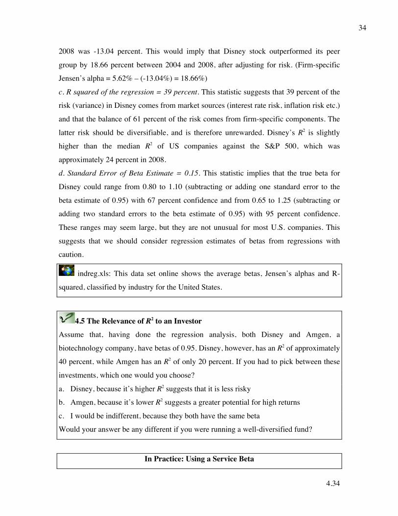
4.34

34

2008 was -13.04 percent. This would imply that Disney stock outperformed its peer

group by 18.66 percent between 2004 and 2008, after adjusting for risk. (Firm-specific

Jensen’s alpha = 5.62% – (-13.04%) = 18.66%)

c. R squared of the regression = 39 percent. This statistic suggests that 39 percent of the

risk (variance) in Disney comes from market sources (interest rate risk, inflation risk etc.)

and that the balance of 61 percent of the risk comes from firm-specific components. The

latter risk should be diversifiable, and is therefore unrewarded. Disney’s R2 is slightly

higher than the median R2 of US companies against the S&P 500, which was

approximately 24 percent in 2008.

d. Standard Error of Beta Estimate = 0.15. This statistic implies that the true beta for

Disney could range from 0.80 to 1.10 (subtracting or adding one standard error to the

beta estimate of 0.95) with 67 percent confidence and from 0.65 to 1.25 (subtracting or

adding two standard errors to the beta estimate of 0.95) with 95 percent confidence.

These ranges may seem large, but they are not unusual for most U.S. companies. This

suggests that we should consider regression estimates of betas from regressions with

caution.

indreg.xls: This data set online shows the average betas, Jensen’s alphas and R-

squared, classified by industry for the United States.

4.5 The Relevance of R2 to an Investor Assume that, having done the regression analysis, both Disney and Amgen, a

biotechnology company, have betas of 0.95. Disney, however, has an R2 of approximately

40 percent, while Amgen has an R2 of only 20 percent. If you had to pick between these

investments, which one would you choose?

a. Disney, because it’s higher R2 suggests that it is less risky

b. Amgen, because it’s lower R2 suggests a greater potential for high returns

c. I would be indifferent, because they both have the same beta

Would your answer be any different if you were running a well-diversified fund?

In Practice: Using a Service Beta

4.35

35

Most analysts who use betas obtain them from an estimation service; Merrill

Lynch, Barra, Value Line, S&P, Morningstar, and Bloomberg are some of the well-

known services. All begin with regression betas and make what they feel are necessary

changes to make them better estimates for the future. Although most of these services do

not reveal the internal details of this estimation, Bloomberg is an honorable exception.

The following is the beta calculation page from Bloomberg for Disney, using the same

period as our regression (January 2004 to December 2008).

The regression is a raw return, rather than an excess return regression, and should thus be

directly comparable to the regression in Figure 4.3. Although the time period used in the

two regressions are identical, there are subtle differences. First, Bloomberg uses price

appreciation in the stock and the market index in estimating betas and ignores

dividends.24 This does not make much of a difference for a Disney, but it could make a

difference for a company that either pays no dividends or pays significantly higher

24This is why the intercept in the Bloomberg graph (0.39%) is slightly different from the intercept estimated earlier in the chapter (0.47%). The beta and R2 are identical.

4.36

36

dividends than the market. Second, Bloomberg also computes what they call an adjusted

beta, which is estimated as follows:

Adjusted Beta = Raw Beta (0.67) + 1(0.33)

These weights do not vary across stocks, and this process pushes all estimated betas

toward one. Most services employ similar procedures to adjust betas toward one. In doing

so, they are drawing on empirical evidence that suggests that the betas for most

companies over time tend to move toward the average beta, which is one. This may be

explained by the fact that firms get more diversified in their product mix and client base

as they get larger.

Generally, betas reported by different services for the same firm can be very

different because they use different time periods (some use two years and others five

years), different return intervals (daily, weekly, or monthly), different market indices, and

different post-regression adjustments. Although these beta differences may be troubling,

the beta estimates delivered by each of these services comes with a standard error, and it

is very likely that all of the betas reported for a firm fall within the range of the standard

errors from the regressions.

Illustration 4.4: Estimating Historical Betas for Aracruz, Tata Chemicals and Deutsche

Bank

Aracruz is a Brazilian company, and we can regress returns on the stock against a

Brazilian index, the Bovespa, to obtain risk parameters. The stock also had an ADR listed

on the U.S. exchanges, and we can regress returns on the ADR against a U.S. index to

obtain parameters. Figure 4.4 presents both graphs for the January 2004- December 2008

time period:

4.37

37

Figure 4.4 Estimating Aracruz’s Beta: Choice of Indices

Source: Bloomberg

How different are the risk parameters that emerge from the two regressions? Aracruz has

a beta of 2.89 when the ADR is regressed against the S&P 500, and a beta of only 0.89

when the local listing is regressed against the Bovespa.25 Each regression has its own

problems. The Bovespa is a narrow index dominated by a few liquid stocks and does not

represent the broad spectrum of Brazilian equities. Although the S&P 500 is a broader

index, the returns on the ADR have little relevance to a large number of non-U.S.

investors who bought the local listing. While it may seem intuitive that an emerging

market stock should have a higher beta to reflect its risk, the results are often

unpredictable, with many emerging market ADRs having much lower betas than their

domestic listings.

Deutsche Bank does not have an ADR listed in the United States, but we can

regress returns against a multitude of indices. Table 4.9 presents comparisons of the

results of the regressions of returns on Deutsche Bank against three indices—a German

equity index (DAX), an index of large European companies (FTSE Euro 300), and a

global equity index (Morgan Stanley Capital Index, MSCI).

Table 4.9 Deutsche Bank Risk Parameters: Index Effect

DAX FTSE Euro 300 MSCI

Intercept -1.63% -1.05% -0.48%

25The biggest source of the difference is one month (January 1999). In that month, Aracruz had a return of 133 percent in the São Paulo exchange whereas the ADR dropped by 9.67 percent in the same month. The disparity in returns can be attributed to a steep devaluation in the Brazilian real in that month.

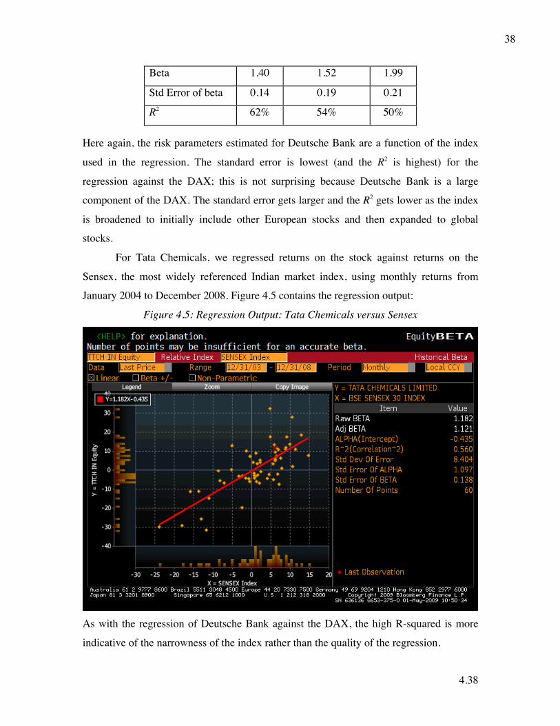
4.38

38

Beta 1.40 1.52 1.99

Std Error of beta 0.14 0.19 0.21

R2 62% 54% 50%

Here again, the risk parameters estimated for Deutsche Bank are a function of the index

used in the regression. The standard error is lowest (and the R2 is highest) for the

regression against the DAX; this is not surprising because Deutsche Bank is a large

component of the DAX. The standard error gets larger and the R2 gets lower as the index

is broadened to initially include other European stocks and then expanded to global

stocks.

For Tata Chemicals, we regressed returns on the stock against returns on the

Sensex, the most widely referenced Indian market index, using monthly returns from

January 2004 to December 2008. Figure 4.5 contains the regression output:

Figure 4.5: Regression Output: Tata Chemicals versus Sensex

As with the regression of Deutsche Bank against the DAX, the high R-squared is more

indicative of the narrowness of the index rather than the quality of the regression.

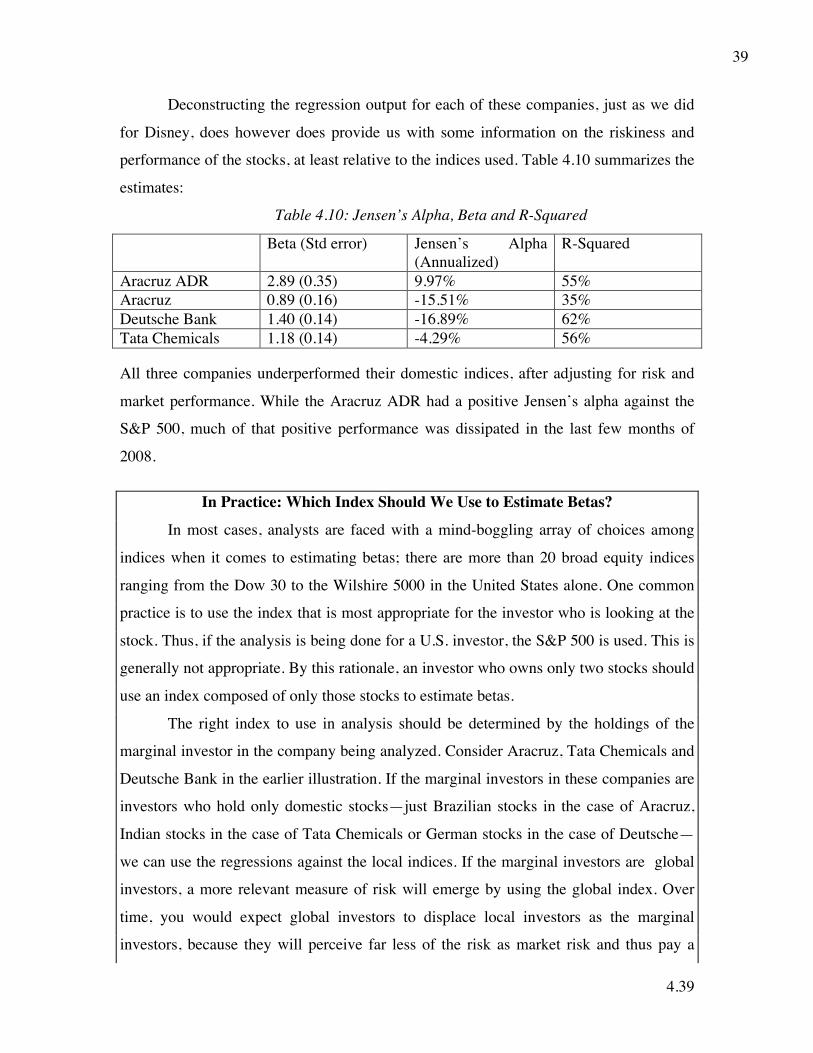
4.39

39

Deconstructing the regression output for each of these companies, just as we did

for Disney, does however does provide us with some information on the riskiness and

performance of the stocks, at least relative to the indices used. Table 4.10 summarizes the

estimates:

Table 4.10: Jensen’s Alpha, Beta and R-Squared

Beta (Std error) Jensen’s Alpha (Annualized)

R-Squared

Aracruz ADR 2.89 (0.35) 9.97% 55% Aracruz 0.89 (0.16) -15.51% 35% Deutsche Bank 1.40 (0.14) -16.89% 62% Tata Chemicals 1.18 (0.14) -4.29% 56%

All three companies underperformed their domestic indices, after adjusting for risk and

market performance. While the Aracruz ADR had a positive Jensen’s alpha against the

S&P 500, much of that positive performance was dissipated in the last few months of

2008.

In Practice: Which Index Should We Use to Estimate Betas?

In most cases, analysts are faced with a mind-boggling array of choices among

indices when it comes to estimating betas; there are more than 20 broad equity indices

ranging from the Dow 30 to the Wilshire 5000 in the United States alone. One common

practice is to use the index that is most appropriate for the investor who is looking at the

stock. Thus, if the analysis is being done for a U.S. investor, the S&P 500 is used. This is

generally not appropriate. By this rationale, an investor who owns only two stocks should

use an index composed of only those stocks to estimate betas.

The right index to use in analysis should be determined by the holdings of the

marginal investor in the company being analyzed. Consider Aracruz, Tata Chemicals and

Deutsche Bank in the earlier illustration. If the marginal investors in these companies are

investors who hold only domestic stocks—just Brazilian stocks in the case of Aracruz,

Indian stocks in the case of Tata Chemicals or German stocks in the case of Deutsche—

we can use the regressions against the local indices. If the marginal investors are global

investors, a more relevant measure of risk will emerge by using the global index. Over

time, you would expect global investors to displace local investors as the marginal

investors, because they will perceive far less of the risk as market risk and thus pay a

4.40

40

higher price for the same security. Thus, one of the ironies of this notion of risk is that

Aracruz will be less risky to an overseas investor who has a global portfolio than to a

Brazilian investor with all of his or her wealth in Brazilian assets.

Standard Procedures for Estimating Risk Parameters in the APM and Multifactor Model

Like the CAPM, the APM defines risk to be nondiversifiable risk, but unlike the

CAPM, the APM allows for multiple economic factors in measuring this risk. Although

the process of estimation of risk parameters is different for the APM, many of the issues

raised relating to the determinants of risk in the CAPM continue to have relevance for the

APM.

The parameters of the APM are estimated

from a factor analysis on historical stock returns,

which yields the number of common economic

factors determining these returns, the risk premium

for each factor, and the factor-specific betas for each

firm.

Once the factor-specific betas are estimated for each firm, and the factor

premiums are measured, the APM can be used to estimated expected returns on a stock.

Cost of Equity = Rf + βj (E(Rj) - Rf)∑j=1

j=k

where

Rf = Risk-free rate

βj = Beta specific to factor j

E(Rj) – Rf = Risk premium per unit of factor j risk

k = Number of factors

In a multifactor model, the betas are estimated relative to the specified factors, using

historical data for each firm.

B. Fundamental Betas

The beta for a firm may be estimated from a regression, but it is determined by

fundamental decisions that the firm has made on what business to be in, how much

operating leverage to use in the business, and the degree to which the firm uses financial

Factor Analysis: This is a statistical

technique in which past data is

analyzed with the intent of extracting

common factors that might have

affected the data.

4.41

41

leverage. In this section, we will examine an alternative way of estimating betas, where

we are less reliant on historical betas and more cognizant of the intuitive underpinnings

of betas.

Determinants of Betas

The beta of a firm is determined by three variables: (1) the type of business or

businesses the firm is in, (2) the degree of operating leverage in the firm, and (3) the

firm’s financial leverage. Much of the discussion in this section will be couched in terms

of CAPM betas, but the same analysis can be applied to the betas estimated in the APM

and the multifactor model as well.

Type of Business Because betas measure the risk of a firm relative to a market index, the

more sensitive a business is to market conditions, the

higher its beta. Thus, other things remaining equal,

cyclical firms can be expected to have higher betas

than noncyclical firms. Other things remaining equal,

then, companies involved in housing and automobiles,

two sectors of the economy that are very sensitive to

economic conditions, will have higher betas than

companies involved in food processing and tobacco, which are relatively insensitive to

business cycles.

Building on this point, we would also argue that the degree to which a product’s

purchase is discretionary will affect the beta of the firm manufacturing the product. Thus,

the betas of discount retailers, such as Wal-Mart, should be lower than the betas of high-

end specialty retailers, such as Tiffany’s or Gucci, because consumers can defer the

purchase of the latter’s products during bad economic times.

It is true that firms have only limited control over how discretionary a product or

service is to their customers. There are firms, however, that have used this limited control

to maximum effect to make their products less discretionary to buyers and by extension

lowered their business risk. One approach is to make the product or service a much more

integral and necessary part of everyday life, thus making its purchase more of a

requirement. A second approach is to effectively use advertising and marketing to build

Cyclical Firm: A cyclical firm has

revenues and operating income that

tend to move strongly with the

economy—up when the economy is

doing well and down during

recessions.

4.42

42

brand loyalty. The objective in good advertising, as we see it, is to make discretionary

products or services seem like necessities to the target audience. Thus corporate strategy,

advertising, and marketing acumen can, at the margin, alter business risk and betas over

time.

4.6 Betas and Business Risk

Polo Ralph Lauren, the upscale fashion designer, went public in 1997. Assume that you

were asked to estimate its beta. Based on what you know about the firm’s products,

would you expect the beta to be

a. greater than one?

b. about one?

c. less than one?

Why?

Degree of Operating Leverage The degree of operating leverage is a function of the cost

structure of a firm and is usually defined in terms of the relationship between fixed costs

and total costs. A firm that has high operating leverage (i.e., high fixed costs relative to

total costs) will also have higher variability in

operating income than would a firm producing a

similar product with low operating leverage.26 Other

things remaining equal, the higher variance in

operating income will lead to a higher beta for the

firm with high operating leverage.

Although operating leverage affects betas, it is difficult to measure the operating

leverage of a firm, at least from the outside, because fixed and variable costs are often

aggregated in income statements. It is possible to get an approximate measure of the

operating leverage of a firm by looking at changes in operating income as a function of

changes in sales.

26To see why, compare two firms with revenues of $100 million and operating income of $10 million, but assume that the first firm’s costs are all fixed, whereas only half of the second firm’s costs are fixed. If revenues increase at both firms by $10 million, the first firm will report a doubling of operating income (from $10 to $20 million), whereas the second firm will report a rise of 55 percent in its operating income (because costs will rise by $4.5 million, 45 percent of the revenue increment).

Operating Leverage: A measure of the

proportion of the operating expenses

of a company that are fixed costs.

4.43

43

Degree of Operating Leverage = % Change in Operating Profit/% Change in Sales

For firms with high operating leverage, operating income should change more than

proportionately when sales change, increasing when sales increase and decreasing when

sales decline.

Can firms change their operating leverage? Although some of a firm’s cost

structure is determined by the business it is in (an energy utility has to build costly power

plants, and airlines have to lease expensive planes), firms in the United States have

become increasingly inventive in lowering the fixed cost component in their total costs.

Labor contracts that emphasize flexibility and allow the firm to make its labor costs more

sensitive to its financial success; joint venture agreements, where the fixed costs are

borne by someone else; and subcontracting of manufacturing, which reduces the need for

expensive plant and equipment, are only some of the manifestations of this phenomenon.

The arguments for such actions may be couched in terms of competitive advantages and

cost flexibility, but they do reduce the operating leverage of the firm and its exposure to

market risk.

Illustration 4.5: Measuring Operating Leverage for Disney

In Table 4.11, we estimate the degree of operating leverage for Disney from 1987

to 2008 using earnings before interest and taxes (EBIT) as the measure of operating

income.

4.44

44

Table 4.11 Degree of Operating Leverage: Disney

Source: Bloomberg

The degree of operating leverage changes dramatically from year to year, because of

year-to-year swings in operating income. Using the average changes in sales and

operating income over the period, we can compute the operating leverage at Disney:

Operating Leverage = % Change in EBIT/% Change in Sales

= 13.26%/13.73% = 0.97

There are two important observations that can be made about Disney over the period,

though. First, the operating leverage for Disney is lower than the operating leverage for

other entertainment firms, which we computed to be 1.15.27 This would suggest that

Disney has lower fixed costs than its competitors. Second, the acquisition of Capital

27To compute this statistic, we looked at the aggregate revenues and operating income of entertainment companies each year from 1987 to 2008.

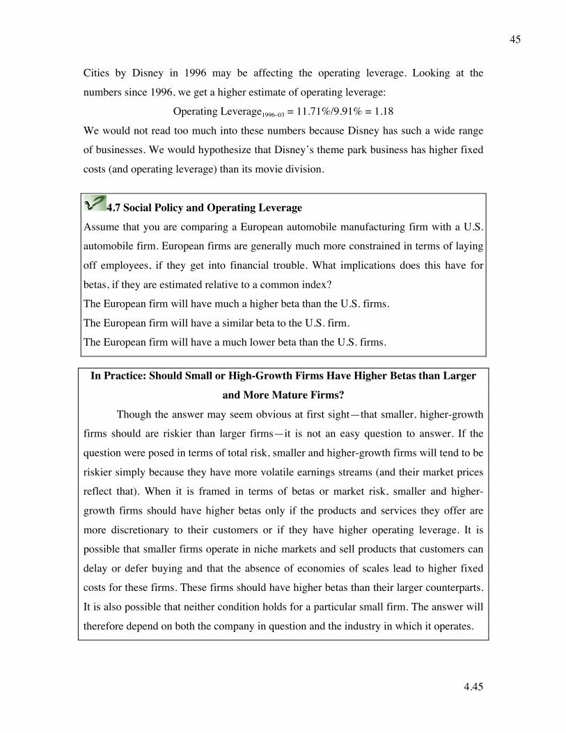
4.45

45

Cities by Disney in 1996 may be affecting the operating leverage. Looking at the

numbers since 1996, we get a higher estimate of operating leverage:

Operating Leverage1996–03 = 11.71%/9.91% = 1.18

We would not read too much into these numbers because Disney has such a wide range

of businesses. We would hypothesize that Disney’s theme park business has higher fixed

costs (and operating leverage) than its movie division.

4.7 Social Policy and Operating Leverage Assume that you are comparing a European automobile manufacturing firm with a U.S.

automobile firm. European firms are generally much more constrained in terms of laying

off employees, if they get into financial trouble. What implications does this have for

betas, if they are estimated relative to a common index?

The European firm will have much a higher beta than the U.S. firms.

The European firm will have a similar beta to the U.S. firm.

The European firm will have a much lower beta than the U.S. firms.

In Practice: Should Small or High-Growth Firms Have Higher Betas than Larger

and More Mature Firms?

Though the answer may seem obvious at first sight—that smaller, higher-growth

firms should are riskier than larger firms—it is not an easy question to answer. If the

question were posed in terms of total risk, smaller and higher-growth firms will tend to be

riskier simply because they have more volatile earnings streams (and their market prices

reflect that). When it is framed in terms of betas or market risk, smaller and higher-

growth firms should have higher betas only if the products and services they offer are

more discretionary to their customers or if they have higher operating leverage. It is

possible that smaller firms operate in niche markets and sell products that customers can

delay or defer buying and that the absence of economies of scales lead to higher fixed

costs for these firms. These firms should have higher betas than their larger counterparts.

It is also possible that neither condition holds for a particular small firm. The answer will

therefore depend on both the company in question and the industry in which it operates.

4.46

46

In practice, analysts often add what is called a small firm premium to the cost of

equity for smaller firms. This small firm premium is usually estimated from historical

data and is the difference between the average annual returns on small market cap stocks

and the rest of the market—about 3 to 3.5 percent when we look at the 1926–2008 period.

This practice can be dangerous for three reasons. The first is that the small firm premium

has been volatile and disappeared for an extended period in the 1980s. The second is that

the definition of a small market cap stock varies across time and that the historical small

cap premium is largely attributable to the smallest (among the small cap) stocks. The

third is that using a constant small stock premium adjustment removes any incentive that

the analyst may have to examine the product characteristics and operating leverage of

individual small market cap companies more closely.

Degree of Financial Leverage Other things remaining equal, an increase in financial

leverage will increase the equity beta of a firm. Intuitively, we would expect that the

fixed interest payments on debt to increase earnings per share in good times and to push it

down in bad times.28 Higher leverage increases the variance in earnings per share and

makes equity investment in the firm riskier. If all of the firm’s risk is borne by the

stockholders (i.e., the beta of debt is zero),29 and debt creates a tax benefit to the firm,

then

βL = βu (1 + (1 – t)(D/E))

where

βL = Levered beta for equity in the firm

βu = Unlevered beta of the firm (i.e., the beta of the assets of the firm)

t = Marginal tax rate for the firm

D/E = Debt/equity ratio

The marginal tax rate is the tax rate on the last dollar of income earned by the firm and

generally will not be equal to the effective or average rates; it is used because interest

28Interest expenses always lower net income, but the fact that the firm uses debt instead of equity implies that the number of shares will also be lower. Thus, the benefit of debt shows up in earnings per share. 29If we ignore the tax effects, we can compute the levered beta as βL = βu (1 + D/E). If debt has market risk (i.e., its beta is greater than zero), the original formula can be modified to take it into account. If the beta of debt is βD, the beta of equity can be written as βL = βu (1 + (1 – t)(D/E)) – βD (1 – t)D/E.

4.47

47

expenses save taxes on the marginal income. Intuitively, we expect that as leverage

increases (as measured by the debt to equity ratio), equity investors bear increasing

amounts of market risk in the firm, leading to higher betas. The tax factor in the equation

captures the benefit created by the tax deductibility of interest payments.

The unlevered beta of a firm is determined by the types of the businesses in which

it operates and its operating leverage. This unlevered beta is often also referred to as the

asset beta because its value is determined by the assets (or businesses) owned by the

firm. Thus, the equity beta of a company is determined both by the riskiness of the

business it operates in as well as the amount of financial leverage risk it has taken on.

Because financial leverage multiplies the underlying business risk, it stands to reason that

firms that have high business risk should be reluctant to take on financial leverage. It also

stands to reason that firms operating in relatively stable businesses should be much more

willing to take on financial leverage. Utilities, for instance, have historically had high

debt ratios but not high betas, mostly because their underlying businesses have been

stable and fairly predictable.

Breaking risk down into business and financial leverage components also

provides some insight into why companies have high betas, because they can end up with

high betas in one of two ways—they can operate in a risky business, or they can use very

high financial leverage in a relatively stable business.

Illustration 4.6: Effects of Financial Leverage on Betas: Disney

From the regression for the period 2004 to 2008, Disney had a beta of 0.95. To

estimate the effects of financial leverage on Disney, we began by estimating the average

debt/equity ratio between 2004 and 2008 using market values for debt and equity.

Average Market Debt/Equity Ratio between 2004 and 2008 = 24.64%

The unlevered beta is estimated using a marginal corporate tax rate of 38%:30

Unlevered Beta = Current Beta/(1 + [1 – tax rate] [Average Debt/Equity])

= 0.95/(1 + [1 – 0.38] [0.2464]) = 0.8241

30The marginal federal corporate tax rate in the United States in 2003 was 35 percent. The marginal state and local tax rates, corrected for federal tax savings, is estimated by Disney in its annual report to be 3% percent. Disney did report some offsetting tax benefits in 2008 that reduced their effective tax rate to 36.1 percent. We assumed that these offsetting tax benefits were temporary.

4.48

48

The levered beta at different levels of debt can then be estimated:

Levered Beta = Unlevered Beta * [1 + (1 – tax rate) (Debt/Equity)]

For instance, if Disney were to increase its debt equity ratio to 10 percent, its equity beta

will be

Levered Beta (@10% D/E) = 0.8241*(1+ (1 – 0.38) (0.10)) = 0.88

If the debt equity ratio were raised to 25 percent, the equity beta would be

Levered Beta (@25% D/E) = 0.8215 *[1 + (1 – 0.38) (0.25)] = 0.95

Table 4.12 summarizes the beta estimates for different levels of financial leverage

ranging from 0 to 90 percent debt.

Table 4.12 Financial Leverage and Betas

Debt to Capital Debt/Equity Ratio Beta Effect of Leverage 0.00% 0.00% 0.82 0.00 10.00% 11.11% 0.88 0.06 20.00% 25.00% 0.95 0.13 30.00% 42.86% 1.04 0.22 40.00% 66.67% 1.16 0.34 50.00% 100.00% 1.34 0.51 60.00% 150.00% 1.59 0.77 70.00% 233.33% 2.02 1.19 80.00% 400.00% 2.87 2.04 90.00% 900.00% 5.42 4.60

As Disney’s financial leverage increases, the beta increases concurrently.

levbeta.xls: This spreadsheet allows you to estimate the unlevered beta for a firm

and compute the betas as a function of the leverage of the firm.

ctrytaxrate.xls: This data set online has marginal tax rates for different countries.

In Practice: Dueling Tax Rates

The marginal tax rate, which is the tax rate on marginal income (or the last dollar

of income) is a key input not only for the levered beta calculation but also for the after-

tax cost of debt, which we will be estimating later in this chapter. Estimating it can be

problematic because firms seldom report it in their financials. Most firms report an

4.49

49

effective tax rate on taxable income in their annual reports and filings with the SEC. This

rate is computed by dividing the taxes paid by the net taxable income, reported in the

financial statement. The effective tax rate can be different from the marginal tax rate for

several reasons.

• If it is a small firm and the tax rate is higher for higher income brackets, the average

tax rate across all income will be lower than the tax rate on the last dollar of income.

For larger firms, where most of the income is at the highest tax bracket, this is less of

an issue.

• Publicly traded firms, at least in the United States, often maintain two sets of books,

one for tax purposes and one for reporting purposes. They generally use different

accounting rules for the two and report lower income to tax authorities and higher

income in their annual reports. Because taxes paid are based on the tax books, the

effective tax rate will usually be lower than the marginal tax rate.

• Actions that defer or delay the payment of taxes can also cause deviations between

marginal and effective tax rates. In the period when taxes are deferred, the effective

tax rate will lag the marginal tax rate. In the period when the deferred taxes are paid,

the effective tax rate can be much higher than the marginal tax rate.

The best source of the marginal tax is the tax code of the country where the firm earns its

operating income. If there are state and local taxes, they should be incorporated into the

marginal tax rate as well. For companies in multiple tax locales, the marginal tax rate

used should be the average of the different marginal tax rates, weighted by operating

income by locale.

Bottom-Up Betas

Breaking down betas into their business, operating leverage, and financial

leverage components provides an alternative way of estimating betas, whereby we do not

need past prices on an individual firm or asset to estimate its beta.

To develop this alternative approach, we need to introduce an additional feature

that betas possess that proves invaluable. The beta of two assets put together is a

weighted average of the individual asset betas, with the weights based on market value.

Consequently, the beta for a firm is a weighted average of the betas of all of different

4.50

50

businesses it is in. Thus, the bottom-up beta for a firm, asset, or project can be estimated

as follows.

1. Identify the business or businesses that make up the firm whose beta we are trying to

estimate. Most firms provide a breakdown of their revenues and operating income by

business in their annual reports and financial filings.

2. Estimate the average unlevered betas of other publicly traded firms that are primarily

or only in each of these businesses. In making this estimate, we have to consider the

following estimation issues:

• Comparable firms: In most businesses, there are at least a few comparable firms

and in some businesses, there can be hundreds. Begin with a narrow definition of

comparable firms, and widen it if the number of comparable firms is too small.

• Beta Estimation: Once a list of comparable firms has been put together, we need

to estimate the betas of each of these firms. Optimally, the beta for each firm will

be estimated against a common index. If that proves impractical, we can use betas

estimated against different indices.

• Unlever First or Last: We can compute an unlevered beta for each firm in the

comparable firm list, using the debt to equity ratio, and tax rate for that firm, or

we can compute the average beta, debt to equity ratio, and tax rate for the sector

and unlever using the averages. Given the standard errors of the individual

regression betas, we would suggest the latter approach.

• Averaging Approach: The average beta across the comparable firms can be either

a simple average or a weighted average, with the weights based on market

capitalization. Statistically, the savings in standard error are larger if a simple

averaging process is used.

• Adjustment for Cash: Investments in cash and marketable securities have betas

close to zero. Consequently, the unlevered beta that we obtain for a business by

looking at comparable firms may be affected by the cash holdings of these firms.

To obtain an unlevered beta cleansed of cash:

€

Unlevered Beta corrected for Cash = Unlevered Beta(1 - Cash/ Firm Value)

4.51

51

The resulting number is sometimes called a pure play beta, indicating that it

measures the risk of only the business and not any other corporate holdings.

3. To calculate the unlevered beta for the firm, we take a weighted average of the

unlevered betas, using the proportion of firm value derived from each business as the

weights. These firm values will have to be estimated because divisions of a firm

usually do not have market values available.31 If these values cannot be estimated, we

can use operating income or revenues as weights. This weighted average is called the

bottom-up unlevered beta. In general, it is good practice to estimate two unlevered

betas for a firm, one for just the operating assets of the firm, and one with cash and

marketable securities treated as a separate business, with a beta of zero.

4. Calculate the current debt to equity ratio for the firm, using market values if available.

Alternatively, use the target debt to equity ratio specified by the management of the

firm or industry-typical debt ratios.

5. Estimate the levered beta for the equity in the firm (and each of its businesses) using

the unlevered beta from Step 3 and the debt to equity ratio from Step 4.

Clearly, this process rests on being able to identify the unlevered betas of individual

businesses.

There are three advantages associated with using bottom-up betas, and they are

significant:

• We can estimate betas for firms that have no price history because all we need is an

identification of the business or businesses they operate in. In other words, we can

estimate bottom-up betas for initial public offerings, private businesses, and divisions

of companies.

• Because the beta for the business is obtained by averaging across a large number of

regression betas, it will be more precise than any individual firm’s regression beta

estimate. The standard error of the average beta estimate will be a function of the

number of comparable firms used in Step 2 and can be approximated as follows:

€

σAverage Beta =Average σ Beta

Number of firms

4.52

52

Thus, the standard error of the average of the betas of 100 firms, each of which has a

standard error of 0.25, will be only 0.025 (0.25/√100).

• The bottom-up beta can reflect recent and even forthcoming changes to a firm’s

business mix and financial leverage, because we can change the mix of businesses

and the weight on each business in making the beta estimate.

Betas.xls: This data set online has updated betas and unlevered betas by business

sector for four groupings – the United States, Europe, Emerging Markets and Japan.

Illustration 4.7: Bottom-Up Beta for Disney

Disney is an entertainment firm with diverse holdings. In addition to its theme

parks, it has significant investments in broadcasting and movies. To estimate Disney’s

beta, we broke their business into four major components:

1. Studio entertainment, which is the production and acquisition of motion pictures for

distribution in theatrical, television, and home video markets as well as TV

programming for network and syndication markets. In addition to the television and

movie productions from Disney Studios, this segment also includes Pixar Studios and

Miramax Studios, with the former specializing in computer animated movies and the

latter on movies for the grown-ups.

2. Media networks, which includes the ABC Television and radio networks and reflects

the acquisition made in 1995. In addition, Disney has an extensive exposure in the

cable market through the Disney channel, A&E, and ESPN, among others.

3. Park resorts, which include Walt Disney World (in Orlando, Florida), Disneyland (in

Anaheim, California) and the recently opened Hong Kong Disney. It also includes

royalty holdings in Tokyo Disneyland and Euro Disney. The hotels at each of these

theme parks are considered part of the parks, because they derive their revenue almost

exclusively from visitors to these parks.

4. Consumer products, which includes a grab-bag of businesses including Disney’s

retail outlets, its licensing revenues, software, interactive products, and publishing.

31The exception is when you have tracking stocks with each division traded separately in financial markets.

4.53

53

This breakdown reflects Disney’s reporting in its annual report. In reality, there are a

number of smaller businesses that Disney is in that are embedded in these four

businesses, including:

• Cruise lines: Disney operates two ships—Disney Magic and Disney Wonder—

that operate out of Florida and visit Caribbean ports.

• Internet operations: Disney made extensive investments in the GO network and

other online operations. Much of this investment was written off by 2002, but

they still represent a potential source of future revenues. In recent years, Disney

has ventured again online and that portion of the business, while small, is

growing.

• Sports franchises: Disney owns the National Hockey League franchise the Mighty

Ducks of Anaheim; in 2002 it sold its stake in the Anaheim Angels, a Major

League Baseball team.

Without detailed information on the operations of these businesses, we will assume that

they represent too small a portion of Disney’s overall revenues to make a significant

difference in the risk calculation. For the four businesses for which we have detailed

information, we estimated the unlevered beta by looking at comparable firms in each

business.32 Table 4.13 summarizes the comparables used and the unlevered beta for each

of the businesses.

Table 4.13 Estimating Unlevered Betas for Disney’s Business Area

To obtain the beta for Disney, we have to estimate the weight that each business is of

Disney as a company. The value for each of the divisions was estimated by applying the

typical revenue multiple at which comparable firm trade at to the revenue reported by

Disney for that segment in 2008.33 The unlevered beta for Disney as a company in 2008

32 We used a 40% marginal tax rate for the comparable firms. 33We first estimated the enterprise value for each firm by adding the market value of equity to the book value of debt and subtracting out cash. We divided the enterprise value by the revenues of each firm to

4.54

54

is a value-weighted average of the betas of each of the different business areas. Table

4.14 summarizes this calculation.

Table 4.14 Estimating Disney’s Unlevered Beta

Business Revenues in

2008 EV/Sales Estimated

Value Firm Value Proportion

Unlevered beta

Media Networks $16,116 2.13 $34,328 58.92% 0.7056 Parks and Resorts $11,504 1.51 $17,408 29.88% 0.5849 Studio Entertainment $7,348 0.78 $5,755 9.88% 1.3027 Consumer Products $2,875 0.27 $768 1.32% 1.0690 Disney Operations $37,843 $58,259 100.00% 0.7333

The equity beta can then be calculated using the current financial leverage for Disney as a

firm. Combining the market value of equity of $45,193 million with an estimated market

value of debt of $16,682 million,34 we arrive at the levered (equity) beta for Disney’s

operating assets:

Debt/Equity Ratio for Disney =

€

$16,682$45,193

= 36.91%

Equity Beta for Disney’s Operating Assets = 0.7333 (1 + (1 – 0.38)(0.3691)) = 0.9011

These are the estimates of unlevered beta and equity beta that we will be using for the

rest of the book, when analyzing operating assets.

We can also compute an unlevered beta for all of Disney’s assets including its

cash holdings and the resulting equity beta:

βDisney=

€

βOperating AssetsValueOperating Assets

(ValueOperating Assets + ValueCash )+ βCash

ValueCash

(ValueOperating Assets + ValueCash )

=

€

0.7333 58,259(58,259 + 3,795)⎛

⎝ ⎜

⎞

⎠ ⎟ + 0

3,795(58,259 + 3,795)⎛

⎝ ⎜

⎞

⎠ ⎟ = 0.6885

Equity BetaDisney as company = 0.6885 (1 + (1 – 0.38)(0.3691)) = 0.8460

obtain the EV/Sales multiple and then used the median value of these estimates. We did not use the averages of these revenue multiples of the individual firms because a few outliers skewed the results. 34The details of this calculation will be explored later in this chapter.

4.55

55

This beta can be compared to the regression beta of 0.95. While it is lower, it is more

precise (because of the averaging) and reflects Disney’s current mix of businesses. There

will be far less call for us to use these cash-adjusted beta values in analyses.35

In Practice: Can’t Find Comparable Firms?

A problem faced by analysts using the bottom-up approach for some firms is a

paucity of comparable firms, either because the company is unique in terms of the

product it offers or because the bulk of the firms in the sector are private businesses.

Rather than fall back on the regression approach, which is likely to yield a very wide

range for the beta, we would suggest one of the following ways to expand the comparable

firm sample.

• Geographic expansion: When analyzing firms from smaller markets, such as Brazil or

Greece, the number of comparable firms will be small if we restrict ourselves only to

firms in the market. One way to increase sample size is to consider firms in the same

business that are listed and traded in other markets—European markets for Greece

and Latin American markets for Brazil. With commodity companies that trade in

global markets, like paper and oil companies, we can consider a global sample.

• Production chain: Another way to expand the sample is to look for firms that either

provide supplies to the firm that you are analyzing or firms that feed off your firm.

For instance, when analyzing book retailers, we can consider book publishers part of

the sample because the fortunes of the two are entwined. It is unlikely that one of

these groups can have a good year without the other partaking in the success.

• Customer specialization: Using the same rationale, the betas of firms that derive the

bulk of their revenues from a sector is best estimated using firms in the sector. Thus,

the beta of a law firm that derives all of its revenues from investment banks can be

estimated by looking at the betas of investment banks.

35 The only setting where these betas will be used is if you are valuing the equity in Disney directly and basing your cash flows on net income (which includes the interest income from the cash). If you are computing a cost of capital to value the operating assets of the firm, you should stick with the betas of just the operating assets.

4.56

56

Illustration 4.8: Bottom-Up Beta for Bookscape Books

We cannot estimate a regression beta for Bookscape Books, the private firm,

because it does not have a history of past prices. We can, however, estimate the beta for

Bookscape Books using the bottom-up approach. Because we were able to find only three

publicly traded book retailers in the United States, we expanded the sample to include

book publishers. We list the betas of these firms as well as debt, cash, and equity values

in Table 4.15.

Table 4.15 Betas and Leverage of Publicly Traded Book Retailers and Publishers Company Name Industry

Name Beta D/E

Ratio Unlevered Beta

Cash/Firm Value

Unlevered beta corrected for cash

Courier Corp. Publishing 0.98 12.33% 0.91 0.46% 0.92 Educational Devel.

Publishing 0.57 0.00% 0.57 15.38% 0.67

McGraw-Hill Ryerson Ltd.

Publishing 0.26 0.00% 0.26 46.97% 0.49

Meredith Corp. Publishing 1.37 66.85% 0.98 3.11% 1.01 Presstek Inc. Publishing 1.68 41.09% 1.35 10.83% 1.51 PRIMEDIA Inc Publishing 1.65 340.84% 0.54 9.20% 0.60 Scholastic Corp. Publishing 1.13 84.49% 0.75 13.36% 0.87 Torstar 'B' Publishing 0.48 54.21% 0.36 4.93% 0.38 Wiley (John) & Sons

Publishing 1.03 52.73% 0.78 1.93% 0.80

Barnes & Noble Retail (Special Lines)

1.34 0.00% 1.34 48.46% 2.60

Books-A-Million Retail (Special Lines)

1.98 97.49% 1.25 7.90% 1.36

Borders Group Retail (Special Lines)

2.44 240.87% 1.00 7.78% 1.08

Median 1.235 53.47% 0.94 8.55% 1.02

Although the firms in this sample are very different in terms of market capitalization, the

betas are consistent. To estimate the unlevered beta for the sector, we first unlevered the

beta for each firm and corrected each unlevered beta for the firm’s cash holdings. The

median value for the unlevered beta, corrected for cash holdings, is 1.02.36

36 Alternate approaches for estimating the beta yielded similar values, with aggregate values for debt, equity and cash generating an unlevered beta of 1.00 for the sector and simple averages for the beta, debt to equity ratio and cash to firm value across the firms provided an estimate of 0.97 for the beta.

4.57

57

Because the debt/equity ratios used in computing levered betas are market debt

equity ratios, and the only debt equity ratio we can compute for Bookscape is a book

value debt equity ratio, we have assumed that Bookscape is close to the book industry

median debt to equity ratio of 53.47 percent. Using a marginal tax rate of 40 percent for

Bookscape, we get a levered beta of 1.35.

Levered beta for Bookscape = 1.02 [1 + (1 – 0.40) (0.5347)] = 1.35

Illustration 4.9: Bottom-Up Beta for Aracruz & Tata Chemicals

The bottom-up beta for Aracruz is difficult to estimate if we remain within its

home market (Brazil) for two reasons. First, there are only three publicly traded firms

within the market that are in the same line of business as Aracruz (i.e., paper and pulp

production). Second, the betas for all Brazilian firms are unreliable because the index

used to estimate these betas, the Bovespa, is a narrow one, dominated by a few large

companies. There are three groups of comparable firms that we can use as comparable

firms in the bottom-up beta estimate:

• Emerging market paper and pulp companies: This is a much larger sample of firms.

Although the individual firm betas may be skewed by the limitations of the local

indices, the errors should average out over the sample.

• U.S. paper and pulp companies: The advantage gained is not just in terms of the

number of firms but also in terms of reliable betas. The peril in this approach is that

the risk in U.S. companies can be different from the risk in Brazilian because of

regulatory differences.37

• Global paper and pulp companies: This is the largest group and includes a diverse

group of companies in both emerging and developed markets. Because betas are

measures of relative risk, we argue that barring significant differences in regulation

and monopoly power across markets, it is reasonable to compare betas across

markets.

The bottom-up betas estimated with each group are summarized in table 4.16.

Table 4.16 Bottom up Beta- Paper and Pulp Business

4.58

58

Number of firms

Median Beta

Median D/E

Median Unlevered Beta Cash/Value

Unlevered Beta Corrected for Cash

Emerging Markets 46 1.03 4.47% 1.00 0.74% 1.01 US 13 1.16 92.29% 0.75 2.87% 0.77 Global 111 0.91 9.82% 0.86 1.24% 0.87

The tax rates used were 32 percent for emerging market companies, 40 percent for U.S.

companies, and 35 percent for global companies, based on averaging the marginal tax

rates in each group. The unlevered beta of emerging market companies is higher than the

U.S. and global groupings. Although the average beta for U.S. companies is higher than

the rest of the sample, this can be attributed to the higher debt to equity ratios of these

companies. We will use an emerging market unlevered beta of 1.01 as the beta for the

paper and pulp business in which Aracruz is involved.

When computing the levered beta for Aracruz’s paper and pulp business, we used

the gross debt outstanding of 9,805 million BR and the market value of equity of 8907

million BR, in conjunction with the marginal tax rate of 34% for Brazil:

Gross Debt to Equity ratio = Debt/Equity = 9805/8907 = 110.08%

Levered Beta for Aracruz Paper business = 1.01 (1+(1-.34)(1.1008)) = 1.74

As with Disney, we can compute a beta for Aracruz as a company, including its cash

balance, and an equity beta based upon this computation. At the end of 2008, the firm had

a negligible cash holding of 20 million BR, thus making almost no difference to the

estimate.

Tata Chemicals is in two businesses – diversified chemicals and fertilizers. To

compute the bottom-up beta for Tata Chemicals, we faced a similar choice of using just

Indian companies, emerging market companies or globally listed companies. As with

Aracruz, we decided to go with the emerging market companies as our comparable firms.

Table 4.17 summarizes the revenues that Tata Chemicals generates from its two

businesses, our estimates of value for each business (based upon the multiples of

37As a counterpoint, paper and pulp companies are commodity companies and are governed by the vagaries of the price of paper and pulp. In other words, there is a reasonable argument to be made that paper and pulp companies globally are governed by the same primary risk factors.

4.59

59

revenues that comparable companies trade at) and the unlevered beta for each business

and for all of Tata Chemicals’ operating assets:

Table 4.17: Beta for Tata Chemicals: Divisions and Company Business(# of comparables)

Revenues (millions)

EV/Sales (from comparable firms)

Estimated Value (millions)

Weights Unlevered Beta

D/E Ratio

Levered Beta

Fertilizers (105)

INR 2,506 1.28 INR 3,208 62.18% 0.72 51.56% 0.965

Chemicals (31)

INR 1,586 1.23 INR 1,951 37.82% 0.68 51.56% 0.911

Tata Chemicals INR 5,158 0.70 0.945

We used the marginal tax rates of 33.99% for India in levering the betas.

In Practice: Gross Debt or Net Debt

Many analysts in Europe and Latin America prefer to subtract the cash from the

gross debt to arrive at a net debt figure, which they then use in both levering betas and in

computing cost of capital.

Net Debt = Gross Debt – Cash and Marketable Securities

The rationale for this netting is that the presence of cash reduces the effective debt burden

of the firm.

We have no quarrel with that logic. In fact, there are two ways, we can reflect the

presence of cash in the levered beta of equity of a firm. In the gross debt approachm the

unlevered beta for a firm (as opposed to just the operating assets of the firm) is a

weighted average of the unlevered beta of its operations and the unlevered beta of its cash

holdings. If we make the assumption that cash has a beta of 0, the unlevered beta for the

firm:

Unlevered BetaFirm = 0 (Cash/ Firm Value) + Unlevered BetaOperations(1-Cash/ Firm Value)

We can then apply the gross debt to equity ratio to this unlevered beta to arrive at the

levered beta of equity. In the net debt approach, we ignore cash while computing the

unlevered beta for the firm, but then lever that beta, using the net debt to equity ratio.

Consider a simple example of a chemical company with $80 million in operating

assets and $ 20 million in cash, funded with $ 60 million in equity and $ 40 million in

debt. Assume that the unlevered beta of the chemical business is 1.20 and that the

marginal tax rate is 40%. First, compute betas using the gross debt approach:

4.60

60

Unlevered BetaCompany = 0 (20/100) + 1.20 (80/100) = 0.96

Gross Debt to Equity Ratio = 40/ 60 = 0.6667

Levered beta = 0.96 (1+ (1-.40) (0.6667)) = 1.344

Now, let’s try the net debt approach.

Unlevered BetaCompany = 1.20

Net Debt to Equity Ratio = (Debt-Cash)/ Equity = (40-20)/ 60 = 0.3333

Levered beta = 1.20 (1+ (1-.40) (0.3333)) = 1.44

Notice that the levered beta of 1.344, computed using the gross debt to equity ratio

approach, does not match the computation using the net debt to equity ratio. The reason

lies in an implicit assumption that we make when we net cash against debt. We assume

that both debt and cash are riskless and that the tax benefit from debt is exactly offset by

the tax paid on interest earned on cash. It is generally not a good idea to net debt if the

debt is very risky or if the interest rate earned on cash is substantially lower than the

interest rate paid on debt. With a net debt to equity ratio, there is one more potential

complication. Any firm that has a cash balance that exceeds its debt will have negative

net debt and using this negative net D/E ratio will yield an unlevered beta that exceeds

the levered beta. Although this may trouble some, it makes sense because the unlevered

beta reflects the beta of the business that the firm operates in. Firms that have vast cash

balances that exceed their borrowing can have levered betas that are lower than the

unlevered betas of the businesses they operate in.

Illustration 4.10: Bottom-Up Beta for Deutsche Bank

There are a few banks in Germany that can be viewed as competitors to Deutsche

Bank, though none of them are as large as it is or have as large of a stake in investment

banking. Because the rules and regulatory constraints governing banking in the United

States are different from the rules governing banks in much of Europe, we will look at the

betas of diversified European banks to estimate the beta for the commercial banking arm

of Deutsche Bank. To estimate the beta of Deutsche Bank’s investment banking arm, we

4.61

61

use the betas of investment banking and brokerage firms, listed in the United States.38

The results are presented in table 4.18:

Table 4.18: Beta for Deutsche Bank

Business Comparable firms Number Average Beta Weights Commercial banking Diversified European Banks 90 1.05 65% Investment Banking US investment banks 32 1.37 35% Deutsche Bank 1.162

Note that we do not adjust for differences in financial leverage, because regulatory

constraints and the needs of the business keep the leverage of most commercial banks at

similar levels.39 The beta for Deutsche Bank as a firm can be estimated as a weighted

average of these two betas, using estimated value weights of 65 percent for the

commercial banking and 35 percent for the investment banking arms, based on the

revenues that Deutsche Bank made from each in the most recent year.

Calculating Betas after a Major Restructuring

The bottom-up process of estimating betas provides a solution when firms go

through a major restructuring, where they change both their business mix and leverage. In

these cases, the regression betas are misleading because they do not fully reflect the

effects of these changes. Disney’s beta, estimated from the bottom-up approach, is likely

to provide a more precise estimate than the beta from a regression, given Disney’s

changing business mix and its increase in financial leverage in recent years. In fact, a

firm’s beta can be estimated even before the restructuring becomes effective using this

approach. In the illustration that follows, for instance, we estimate Disney’s beta just

before and after its acquisition of Capital Cities/ABC in 1995, allowing for the changes in

both the business mix and the leverage.

Illustration 4.11: Beta of a Firm after an Acquisition: Disney/Capital Cities

In 1995, Disney announced that it was acquiring Capital Cities, the owner of the

ABC television and radio network, for approximately $120 per share, and that it would

38 In much of the rest of the world, investment banking is an arm of commercial banking rather than a stand-alone operation. 39Regulators often specify capital ratios, specified in terms of book values of debt and equity that banks must meet to stay in business. Most banks stay close to these ratios, though some tend to be better capitalized than others.

4.62

62

finance the acquisition partly through the issue of $10 billion in debt. At the time of the

acquisition, Disney had a market value of equity of $31.1 billion, debt outstanding of

$3.186 billion, and a levered beta of 1.15. Capital Cities, based on the $120 offering

price, had a market value of equity of $18.5 billion, debt outstanding of $615 million, and

a levered beta of 0.95.

To evaluate the effects of the acquisition on Disney’s beta, we do the analysis in

two parts. First, we examine the effects of the merger on the business risk of the

combined firm, by estimating the unlevered betas of the two companies, and calculating

the combined firm’s unlevered beta (using a tax rate of 36% for both firms).

Disney’s unlevered beta = 1.15/(1 + (1-.36)*(3,186/31,100)) = 1.08

Capital Cities unlevered beta = 0.95/(1 + (1-.36)*(615/18500)) = 0.93

The unlevered beta for the combined firm can be calculated as the weighted average of

the two unlevered betas, with the weights being based upon the market values of the two

firms.40

Value of Disney = $31,100 + $3,186 = $34,286 million

Value of Capital Cities = $18,500 + $ 615 = $19,115 million

Unlevered Beta for combined firm = 1.08 (34,286/53,401) + 0.93 (19,115/53,401)

= 1.026

Then we examine the effects of the financing of the merger on the betas by calculating

the debt/equity ratio for the combined firm after the acquisition. Because Disney is

assuming the old debt of Capital Cities, we add that debt to Disney’s existing debt and

add the additional $10 billion in debt used to fund this acquisition:41

Post-acquisition Debt = Capital Cities Old Debt + Disney’s Old Debt + New Debt

= $615 + $3,186 + $10,000 = $13,801 million

Post-acquisition Equity = Disney’s Old Equity + New Equity Used for Acquisition

= $31,100 + $8,500 = $39,600 million

where New Equity = Total Cost of Acquisition – New Debt Issued

40Unlevered betas should always be weighted based on firm values. With levered (equity) betas, the values of equity can be used as weights. 41If Disney had paid off Capital Cities’ existing debt instead of assuming it, we could have ignored it in the debt calculation. However, Disney would then have had to raise an extra $615 million in financing to fund this acquisition.

4.63

63

= $18,500 – $10,000 = $8,500 million

Notice that the equity in Capital Cities of $18,500 million disappears after the acquisition

and is replaced with new debt of $10,000 million and new Disney equity of $8,500

million. The debt/equity ratio can then be computed as follows.

D/E Ratio = 13,801/39600 = 34.82%

This debt/equity ratio in conjunction with the new unlevered beta for the combined firm

yields a new beta of

New Beta = 1.026 (1 + 0.64 (.3482)) = 1.25

Based on this computation, we would expect Disney’s beta to increase from 1.15 to 1.25

after the acquisition of Capital Cities.

C. Accounting Betas

A third approach is to estimate the beta of a firm or its equity from accounting

earnings rather than from traded prices. Thus, changes in earnings at a division or a firm,

on a quarterly or annual basis, can be regressed against changes in earnings for the

market, in the same periods, to arrive at an estimate of a “market beta” to use in the

CAPM. The approach has some intuitive appeal, but it suffers from three potential

pitfalls. First, accounting earnings tend to be smoothed out relative to the underlying

value of the company, resulting in betas that are “biased down,” especially for risky

firms, or “biased up,” for safer firms. In other words, betas are likely to be closer to one

for all firms using accounting data. Second, accounting earnings can be influenced by

non-operating factors, such as changes in depreciation or inventory methods, and by

allocations of corporate expenses at the division level. Finally, accounting earnings are

measured, at most, once every quarter, and often only once every year, resulting in

regressions with few observations and not much power.

Illustration 4.12: Estimating Accounting Betas: Bookscape Books

Bookscape Books, even though it is a private business, has been in existence since

1980 and has accounting earnings going back to that year. Table 4.19 summarizes

accounting earnings changes at Bookscape and for companies in the S&P 500 for each

year since 1980.

Table 4.19: Change in Earnings (%) for Bookscape versus S&P 500

4.64

64

Year S&P 500 Bookscape Year S&P 500 Bookscape 1980 3.01% 3.55% 1995 18.74% 11.55% 1981 1.31% 4.05% 1996 7.77% 19.88% 1982 -8.95% -14.33% 1997 8.52% 16.55% 1983 -3.84% 47.55% 1998 0.41% 7.10% 1984 26.69% 65.00% 1999 16.74% 14.40% 1985 -6.91% 5.05% 2000 8.61% 10.50% 1986 -7.93% 8.50% 2001 -30.79% -8.15% 1987 11.10% 37.00% 2002 18.51% 4.05% 1988 50.42% 45.17% 2003 18.79% 12.56% 1989 0.83% 3.50% 2004 23.75% 14.50% 1990 -6.87% -10.50% 2005 12.96% 8.35% 1991 -14.79% -32.00% 2006 14.74% 16.74% 1992 8.13% 55.00% 2007 -5.91% 2.50% 1993 28.89% 31.00% 2008 -20.78% -12.20% 1994 18.03% 21.06%

Regressing the changes in profits at Bookscape against changes in profits for the S&P

500 yields the following:

Bookscape Earnings Change = 0.08 + 0.8211 (S&P 500 Earnings Change)

Based on this regression, the beta for Bookscape is 0.82. In calculating this beta, we used

net income to arrive at an equity beta. Using operating earnings for both the firm and the

S&P 500 should yield the equivalent of an unlevered beta.

Technically, there is no reason why we cannot estimate accounting betas for

Disney, Aracruz Cellulose, Tata Chemicals and Deutsche Bank. In fact, for Disney, we

could get net income numbers every quarter, which increases the data we have in the

regression. We could even estimate accounting betas by division, because the divisional

income is reported. We do not attempt to estimate accounting betas for the following

reasons:

1. To get a sufficient number of observations in our regression, we would need to go

back in time at least ten years and perhaps more. The changes that many large

companies undergo over time make this a hazardous exercise.

2. Publicly traded firms smooth out accounting earnings changes even more than private

firms do. This will bias the beta estimates downward.

4.65

65

spearn.xls: This data set online has earnings changes, by year, for the S&P 500

going back to 1960.

Market, Fundamental, and Accounting Betas: Which One Do We Use?

For most publicly traded firms, betas can be estimated using accounting data,

market data, or fundamentals. Because the betas will almost never be the same, the

question then becomes one of choosing between them. We would almost never use

accounting betas for all of the reasons already specified. We are almost as reluctant to use

historical market betas for individual firms because of the standard errors in beta

estimates, the failures of the local indices, and the inability of these regressions to reflect

the effects of major changes in the business and financial risk at the firm. Fundamental

betas, in our view, provide the best beta estimates because they not only are more precise

(because of the averaging) but also allow us to reflect changes in business and financial

mix. In summary, we will use the fundamental estimates of equity betas, based upon the

operating assets, of 0.90 for Disney, 0.94 for Tata Chemicals, 1.35 for Bookscape, 1.74

for Aracruz, and 1.16 for Deutsche Bank.

IV. Estimating the Cost of Equity Having estimated the risk-free rate, the risk premium(s), and the beta(s), we can

now estimate the expected return from investing in equity at any firm. In the CAPM, this

expected return can be written as:

Expected Return = Risk-Free Rate + Beta * Expected Risk Premium

where the risk-free rate would be the rate on a long-term government bond; the beta

would be either the historical, fundamental, or accounting betas; and the risk premium

would be either the historical premium or an implied premium.

In the APM and multifactor model, the expected return would be written as

follows:

Expected Return = Risk-free Rate + βjj−1

j= n

∑ * Risk Premiumj

4.66

66

where the risk-free rate is the long term government bond rate, βj is the beta relative to

factor j, estimated using historical data or fundamentals, and Risk Premiumj is the risk

premium relative to factor j, estimated using historical data.

The expected return on an equity investment in a firm, given its risk, has key

implications for both equity investors in the firm and the managers of the firm. For equity

investors, it is the rate they need to make to be compensated for the risk that they have

taken on investing in the equity of a firm. If after analyzing a stock, they conclude that

they cannot make this return, they would not buy it; alternatively, if they decide they can

make a higher return, they would make the investment. For managers in the firm, the

return that investors need to make to break even on their equity investments becomes the

return that they have to try to deliver to keep these investors from becoming restive and

rebellious. Thus, it becomes the rate that they have to beat in terms of returns on their

equity investments in individual projects. In other words, this is the cost of equity to the

firm.

Illustration 4.13: Estimating the Cost of Equity

In Illustration 4.7, we estimated a bottom-up unlevered beta for Disney and each

of its divisions. To estimate the levered beta for Disney, we estimated a debt to equity

ratio of 36.91%, based upon the total market value of equity ($45,193 million) and debt

($16,682 million). To estimate the levered beta for each of the divisions, we face a

challenge in determining the debt to equity ratio at the divisional level, since we do not

have market equity values for the individual divisions nor do we have full details on

which divisions are responsible for the borrowing. We have two choices. One is to

assume that Disney debt to equity ratio applies to all of its individual divisions. The other

is to try to make judgments about the debt to equity ratios for the individual divisions,

based upon the information available. In table 4.20, we tried to do the latter:

Table 4.20: Allocating Debt and Equity to divisions

Business Estimated EV

Allocated Debt

Estimated Equity

D/E Ratio

D/E Ratio of comps

Estimated debt Proportions

Media Networks $34,328 $8,582 $25,746 33.33% 38.71% $9,581 51.44% Parks and Resorts $17,408 $6,148 $11,260 54.61% 65.10% $6,864 36.86%

4.67

67

Studio Entertainment $5,755 $1,805 $3,950 45.70% 53.89% $2,015 10.82% Consumer Products $768 $147 $621 23.70% 27.21% $164 0.88% $18,624 100.00%

We started with the estimates of enterprise value that we obtained in table 4.14, obtained

by multiplying the revenues in each division by the median EV/Sales ratio of comparable

companies in the division. We then used the D/E ratios of these same comparable firms to

estimate the debt in each division in the second to last column and used the proportions

derived from these estimated debt numbers to allocate the existing debt ($16,682 million)

across the divisions.42 Finally, we estimated the value of equity in each division by

subtracting the debt from the estimated enterprise value.

Using the US dollar riskfree rate (from illustration 4.1) and the equity risk

premium estimated for mature markets (from illustration 4.2), we estimate the cost of

equity for Disney’s operating assets and for each of its divisions, listed in Table 4.21.

Table 4.21 Levered Beta and Cost of Equity: Disney

Business Unlevered Beta D/E Ratio Levered Beta Cost of Equity Media Networks 0.7056 33.33% 0.8514 8.61% Parks and Resorts 0.5849 54.61% 0.7829 8.20% Studio Entertainment 1.3027 45.70% 1.6718 13.53% Consumer Products 1.0690 23.70% 1.2261 10.86% Disney 0.7333 36.91% 0.9011 8.91%

The costs of equity vary across the remaining divisions, with studio entertainment having

the highest beta (and cost of equity) and parks and resorts the lowest.

To estimate the cost of equity for Deutsche Bank, we will use the same risk

premium (6 percent) that we have used for the United States, because Deutsche Bank’s

business is still primarily in mature markets in Europe and the United States. Using the

ten-year German Euro bond rate of 3.60 percent as the Euro risk-free rate (from

42 Some analysts use the industry average debt to equity ratios to estimate levered betas by division. The problem with doing this is that the sum total of the debt that they estimate for the divisions may not match up to the actual debt of the company. In the case of Disney, for instance, the dollar debt that we would have obtained with this approach ($18,624 million) would have greater than the debt owed by the company ($16,682 million)

4.68

68

illustration 4.1) and Deutsche Bank’s bottom up beta of 1.16, the cost of equity for

Deutsche Bank is shown in Table 4.22.

Table 4.22: Cost of Equity for Deutsche Bank

Business Beta Cost of Equity Commercial banking 1.05 3.6%+1.05 (6%) = 9.90% Investment Banking 1.37 3.6%+1.37 (6%) = 11.82% Deutsche Bank 1.162 3.6%+1.162 (6%) = 10.55%

Note that the cost of equity for investment banking is significantly higher than the cost of

equity for commercial banking, reflecting the higher risks.

For Aracruz, we will add the country risk premium estimated for Brazil of 3.95%

percent, estimated earlier in the chapter, to the mature market premium, estimated from

the United States, of 6 percent to arrive at a total risk premium of 9.95 percent (see

illustration 4.2). The cost of equity for Aracruz can then be computed in US dollar terms

using the bottom-up beta estimated in Illustration 4.9 and the US treasury bond rate of

3.5%:

Cost of EquityUS dollars = Risk-Free Rate$ + Beta * Risk Premium

= 3.5% + 1.74 (9.95%) = 20.82%

Note that we can compute Aracruz’s cost of equity in nominal Brazilian Reals in one of

two ways. The first is to replace the US dollar riskfree rate with a nominal Brazilian Real

riskfere rate (estimated to be 8.5% in illustration 4.1):

Cost of EquityNominal $R = Riskfree RateR$ + Beta* Risk Premium

= 8.5% + 1.74 (9.95%) = 25.82%

This approach assumes that the equity risk premium, which was computed using dollar-

based securities, will stay constant even if we switch to a higher inflation currency. The

second and more precise approach scales up the equity risk premium, when we switch to

the higher inflation currency. If we assume that the expected inflation rate is 7% in

nominal $R and 2% in US $, we obtain:

Cost of EquityNominal R$ = (1+ Cost of EquityUS $)

€

(1+ Expected InflationR$)(1+ Expected InflationUS $)

−1

= (1.2082)

€

(1.07)(1.02)

−1= 26.75%

4.69

69

As an emerging market company with a high debt to equity ratio, Aracruz clearly faces a

much higher cost of equity than its competitors in developed markets.

For Tata Chemicals, we estimate the cost of equity in Indian rupees, using the

rupee riskfree rate of 4% (estimated in illustration 4.1) and the equity risk premium for

India of 10.51% (estimated in illustration 4.2). Table 4.23 summarizes the cost of equity

estimates for the fertilizer and chemical businesses separately, as well as for the entire

company.

Table 4.23: Cost of Equity by division: Tata Chemicals

Business Beta Cost of equity Fertilizers 0.965 4%+ 0.965 (10.51%) = 14.14% Chemicals 0.911 4%+ 0.911(10.51%) = 13.58% Tata Chemicals 0.945 4%+ 0.945 (10.51%) = 13.93%

Finally, for Bookscape, we will use the beta of 1.35 estimated from Illustration

4.8 in conjunction with the risk-free rate and risk premium for the United States:

Cost of Equity = 3.5% + 1.35 (6%) = 11.60%

Implicit in the use of beta as a measure of risk is the assumption that the marginal

investor in equity is a well-diversified investor. Although this is a defensible assumption

when analyzing publicly traded firms, it becomes much more difficult to sustain for

private firms. The owner of a private firm generally has the bulk of his or her wealth

invested in the business. Consequently, he or she cares about the total risk in the business

rather than just the market risk. Thus, for a business like Bookscape, the beta that we

have estimated of 1.35 (leading to a cost of equity of 11.60 percent) will understate the

risk perceived by the owner. There are three solutions to this problem:

1. Assume that the business is run with the near-term objective of sale to a large

publicly traded firm. In such a case, it is reasonable to use the market beta and cost of

equity that comes from it.

2. Add a premium to the cost of equity to reflect the higher risk created by the owner’s

inability to diversify. This may help explain the high returns that some venture

capitalists demand on their equity investments in fledgling businesses.

3. Adjust the beta to reflect total risk rather than market risk. This adjustment is

relatively simple, because the R2 of the regression measures the proportion of the

4.70

70

variance that is market risk. Dividing the market beta by the square root of the R2

(which yields the correlation coefficient) yields a total beta. In the Bookscape

example, the regressions for the comparable firms against the market index have an

average correlation with the market of 46.45% (the average R2 was 21.58%). The

total beta for Bookscape can then be computed as follows:

Total Beta = (Market Beta)/Correlation with the market = 1.35/0.4645= 2.91

Using this total beta would yield a much higher and more realistic estimate of the cost of

equity.

Cost of Equity = 3.5% + 2.91 (6%) = 20.94%

Thus, private businesses will generally have much higher costs of equity than their

publicly traded counterparts, with diversified investors. Although many of them

ultimately capitulate by selling to publicly traded competitors or going public, some firms

choose to remain private and thrive. To do so, they have to diversify on their own (as

many family-run businesses in Asia and Latin America did) or accept the lower value as

a price paid for maintaining total control.

In Practice: Company Exposure to Country Risk

In our computations of cost of equity for companies, note that we attached

country risk premiums to Aracruz (Brazil) and Tata Chemicals (India) and used only a

mature market premium for Disney and Deutsche Bank. While we are following

conventional practice in assessing country risk based upon where a company is

incorporated, it can also lead to misleading values for companies that are incorporated in

an emerging market (developed market) and have a significant portion of their operations

in a developed market (emerging market). This would have been the case, for instance, if

we had been analyzing Embraer, a Brazilian aerospace company with less than 10% of its

revenues from Brazil and the rest from developed markets, or Infosys, an Indian

technology company that derives more than half of its revenues in the United States.

There is a simple (perhaps even simplistic) way of adjusting for operating risk

exposure.43 Rather than use the risk premium of the country of incorporation, we can use

a weighted average of the total risk premiums of the countries in which the company

4.71

71

operates, using revenues as the basis for the weighting. Thus, the equity risk premium

used for a company that derives half its revenues in India and half in the United States

would be:

Equity Risk Premium = (.5) (6%) + (.5) (10.51%) = 8.26%

Thus, the costs of equity of companies like Nestle and Coca Cola, which have substantial

operations in emerging markets, will increase. We did break down Disney’s revenues

geographically and noted that while it does have significant non-US operations, most are

still centered in Western Europe and Japan and thus do not affect the risk premium.

However, as its Hong Kong theme park’s revenues increase, we may have to adjust the

equity risk premium to reflect greater emerging market risk. Tata Chemicals gets almost

90% of its revenues from India and the use of the Indian total risk premium seems

appropriate. We are a little more concerned about our equity risk premium assessments

for Deutsche Bank (which we feel is exposed to more emerging market risk) and Aracruz

(which has significant revenues outside Brazil). However, we made no adjustments

because of the absence of a clear measure of emerging market operations for the former

and the offsetting additional risk of being a natural resource company for the latter.44

From Cost of Equity to Cost of Capital Equity is undoubtedly an important and indispensable ingredient of the financing

mix for every business, but it is only one ingredient. Most businesses finance some or

much of their operations using debt or some hybrid of equity and debt. The costs of these

sources of financing are generally very different from the cost of equity, and the

minimum acceptable hurdle rate for a project will reflect their costs as well, in proportion

to their use in the financing mix. Intuitively, the cost of capital is the weighted average of

the costs of the different components of financing—including debt, equity, and hybrid

securities—used by a firm to fund its financial requirements.

4.8: Interest Rates and the Relative Costs of Debt and Equity

43 For more comprehensive ways of estimating company risk exposure to country risk, see the working paper on my web site: Damodaran, A., 2003, Estimating Company Risk Exposure to Country Risk. 44 Natural resource companies are particularly exposed to country risk, because they do not have the option of moving operations if the country that their resources are in is in trouble. Manufacturing companies can move their factories to more stable locations but oil, mining and forestry companies cannot.

4.72

72

It is often argued that debt becomes a more attractive mode of financing than equity as

interest rates go down and a less attractive mode when interest rates go up. Is this

true?

a. Yes

b. No

Why or why not?

The Costs of Non-equity Financing

To estimate the cost of the funding that a firm raises,

we have to estimate the costs of all of the non-equity

components. In this section, we consider the cost of debt

first and then extend the analysis to consider hybrids, such

as preferred stock and convertible bonds.

The Cost of Debt

The cost of debt measures the current cost to the firm of borrowing funds to

finance projects. In general terms, it is determined by the following variables:

1. The current level of interest rates: As market interest rates rise, the cost of debt for all

firms will also increase.

2. The default risk of the company: As the default risk of a firm increases, lenders will

charge higher interest rates (a default spread) to compensate for the additional risk.

3. The tax advantage associated with debt: Because interest is tax-deductible, the after-

tax cost of debt is a function of the tax rate. The tax benefit that accrues from paying

interest makes the after-tax cost of debt lower than the pretax cost. Furthermore, this

benefit increases as the tax rate increases.

After-Tax Cost of Debt = (Riskfree rate + Default Spread) (1 – Marginal Tax Rate)

The challenge in estimating cost of debt is really one of estimating the correct default

spread for a company.

4.9: Costs of Debt and Equity

Can the cost of equity ever be lower than the cost of debt for any firm at any stage in its

life cycle?

Default Risk: The risk that a firm

will fail to make obligated debt

payments, such as interest

expenses or principal payments.

4.73

73

Yes

No

Estimating the Default Risk and Default Spread of a Firm

The simplest scenario for estimating the cost of debt occurs when a firm has long-

term bonds outstanding that are widely traded and have no special features, such as

convertibility or first claim on assets, skewing interest rates. The market price of the

bond, in conjunction with its coupon and maturity, can serve to compute a yield we use as

the cost of debt. For instance, this approach works for firms that have dozens of

outstanding bonds that are liquid and trade frequently.

Many firms have bonds outstanding that do not trade on a regular basis. Because

these firms are usually rated, we can estimate their costs of debt by using their ratings and

associated default spreads. Thus, Disney with an A rating can be expected to have a cost

of debt approximately 2.5 percent higher than the Treasury bond rate, in May 2009,

because this was the spread typically paid by A rated firms at the time.

Some companies choose not to get rated. Many smaller firms and most private

businesses fall into this category. Ratings agencies have sprung up in many emerging

markets, but there are still a number of markets in which companies are not rated on the

basis of default risk. When there is no rating available to estimate the cost of debt, there

are two alternatives:

• Recent Borrowing History: Many firms that are not rated still borrow money from

banks and other financial institutions. By looking at the most recent borrowings

made by a firm, we can get a sense of the types of default spreads being charged

and use these spreads to come up with a cost of debt.

• Estimate a Synthetic Rating and Default Spread: An alternative is to play the role

of a ratings agency and assign a rating to a firm based on its financial ratios; this

rating is called a synthetic rating. To make this assessment, we begin with rated

firms and examine the financial characteristics shared by firms within each ratings

class. Consider a very simpler version, where the ratio of operating income to

interest expense, that is, the interest coverage ratio, is computed for each rated

firm. In Table 4.24, we list the range of interest coverage ratios for manufacturing

4.74

74

firms in each S&P ratings class, classified by market capitalization into large (>$5

billion) and small (<$5 billion).45 We also report the typical default spreads for

bonds in each ratings class in early 2009.46

Table 4.24 Interest Coverage Ratios and Ratings

Interest Coverage Ratio: Small market cap(<$5 billion)

Interest Coverage Ratio: Large market cap (>US $ 5 billion)

Rating Typical Default

> 12.5 >8.5 AAA 1.25% 9.50–12.50 6.5-8.5 AA 1.75% 7.50–9.50 5.5-6.5 A+ 2.25% 6.00–7.50 4.25- 5.5 A 2.50% 4.50–6.00 3- 4.25 A– 3.00% 4.00-4.50 2.5-3.0 BBB 3.50% 3.50–4.00 2.25-2.5 BB+ 4.25% 3.00–3.50 2.0-2.25 BB 5.00% 2.50–3.00 1.75-2.0 B+ 6.00% 2.00–2.50 1.5-1.75 B 7.25% 1.50–2.00 1.25-1.5 B– 8.50% 1.25–1.50 0.8-1.25 CCC 10.00% 0.80–1.25 0.65-0.8 CC 12.00% 0.50–0.80 0.2-0.65 C 15.00%

< 0.65 <0.2 D 20.00% Source: Compustat and Bondsonline.com.

Now consider a private firm with $10 million in earnings before interest and taxes and $3

million in interest expenses; it has an interest coverage ratio of 3.33. Based on this ratio,

we would assess a synthetic rating of BB for the firm and attach a default spread of 5.00

percent to the risk-free rate to come up with a pretax cost of debt. A large market cap

firm with the same interest coverage ratio would be assigned a rating of A- and a default

spread of 3.00%.

By basing the synthetic rating on the interest coverage ratio alone, we run two

risks. One is that using last year’s operating income as the basis for the rating may yield

too low or too high a rating for a firm that had an exceptionally good or bad earnings

years. We can counter that by using the average operating income over a period, say 5

45This table was first developed in early 2000, by listing all rated firms with market capitalization lower than $5 billion and their interest coverage ratios, and then sorting firms based on their bond ratings. The ranges were adjusted to eliminate outliers and to prevent overlapping ranges. It has been updated every two years since. 46These default spreads are obtained from an online site, found at www.bondsonline.com. You can find default spreads for industrial and financial service firms; these spreads are for industrial firms.

4.75

75

years, to compute the coverage ratio. The other is that we risk missing the information

that is available in the other financial ratios and qualitative information used by ratings

agencies. The counter to that is to extend the approach to incorporate other ratios. The

first step would be to develop a score based on multiple ratios. For instance, the Altman

z-score, which is used as a proxy for default risk, is a function of five financial ratios,

which are weighted to generate a z-score. The ratios used and their relative weights are

usually based on past history on defaulted firms. The second step is to relate the level of

the score to a bond rating, much as we did in Table 4.24, with interest coverage ratios. In

making this extension, though, note that complexity comes at a cost. Credit or z-scores

may, in fact, yield better estimates of synthetic ratings than those based only on interest

coverage ratios, but changes in ratings arising from these scores are much more difficult

to explain than those based on interest coverage ratios. That is the reason we prefer the

flawed but more transparent ratings from interest coverage ratios.

ratings.xls: This spreadsheet allows you to estimate a synthetic rating for a firm.

In Practice: Debt Betas and Costs of Debt

Given our use of equity betas to compute the cost of equity, you may be wondering

why we cannot use debt betas to compute the pre-tax cost of debt. In other words, instead

of estimating a bond rating for a company and a default spread based upon the rating,

why not estimate a beta for debt, by regressing bond returns against a market index, and

use that beta in the capital asset pricing model to estimate the cost of debt. There are two

reasons why we are reluctant to go down the road:

a. Non-traded debt: Even at large publicly traded companies, a significant portion of the

debt is not traded, thus making it impossible to regress returns against a market index.

b. Asymmetric payoffs: Beta as a measure of risk draws on the mean-variance

framework, which in turn assumes returns that are roughly symmetric, with upside

risk offset by downside risk. When you lend to a firm, your risks tend to be

asymmetric, with your best case scenario being that you get your promised interest

and principal payments and your worst case scenarios containing far worse outcomes.

4.76

76

That is why we focus on downside risk, i.e. default risk, when assessing the cost of

debt for a firm.

It is conceivable that debt begins to have more symmetric payoffs as it gets riskier and

that debt betas may therefore make sense, if we are looking at low rated companies. It is

unlikely that debt betas will be of much use in assessing the cost of debt for most other

firms.

Short-Term and Long-Term Debt

Most publicly traded firms have multiple borrowings—short-term and long-term

bonds and bank debt with different terms and interest rates. Although there are some

analysts who create separate categories for each type of debt and attach a different cost to

each category, this approach is both tedious and dangerous. Using it, we can conclude

that short-term debt is cheaper than long-term debt and that secured debt is cheaper than

unsecured debt.

The solution is simple. Combine all debt—short- and long-term, bank debt and

bonds—and attach the long-term cost of debt to it. In other words, add the default spread

to the long-term risk-free rate and use that rate as the pretax cost of debt. Firms will

undoubtedly complain, arguing that their effective cost of debt is lowered by using short-

term debt. This is technically true, largely because short-term rates tend to be lower than

long-term rates in most developed markets, but it misses the point of computing the cost

of debt and capital. If this is the hurdle rate we want our long-term investments to beat,

we want the rate to reflect the cost of long-term borrowing and not short-term borrowing.

After all, a firm that funds long-term projects with short-term debt will have to return to

the market to roll over this debt.

Operating Leases and Other Fixed Commitments

The essential characteristic of debt is that it gives rise to a tax-deductible

obligation that firms have to meet in both good times and bad, and the failure to meet this

obligation can result in bankruptcy or loss of equity control over the firm. If we use this

definition of debt, it is quite clear that what we see reported on the balance sheet as debt

may not reflect the true borrowings of the firm. In particular, a firm that leases substantial

assets and categorizes them as operating leases owes substantially more than is reported

4.77

77

in the financial statements.47 After all, a firm that signs a lease commits to making the

lease payment in future periods and risks the loss of assets if it fails to make the

commitment.

For corporate financial analysis, we should treat all lease payments as financial

expenses and convert future lease commitments into debt by discounting them back the

present, using the current pretax cost of borrowing for the firm as the discount rate. The

resulting present value can be considered the debt value of operating leases and can be

added on to the value of conventional debt to arrive at a total debt figure. To complete

the adjustment, the operating income of the firm will also have to be restated:

Adjusted Operating Income = Stated Operating Income + Operating Lease

Expense for the Current Year – Depreciation on Leased Asset

To the extent that estimating depreciation on the leased asset can be tedious, an

approximation can also be used:

Adjusted Operating Income = Stated Operating Income + PV of lease commitments *

Pre-tax cost of debt

In effect, we are computing the imputed interest expense on the lease debt and adding it

back to the stated operating income, since it is income before interest expenses. In fact,

this process can be used to convert any set of financial commitments into debt.

To convert leases to debt, we need a listing of all lease commitments into the

future that have already been made; this is required already in the US and is available for

more and more non-US firms. We also need a pre-tax cost of debt to do the discounting.

While this may be simple if the firm has a bond rating, it becomes more complicated if

the firm is not rated. We can try to compute a synthetic rating but will run into a problem

of circularity, since we need interest expenses to compute the rating but we need the

rating to compute the present value of debt and the potential interest expenses from that

debt. There are three solutions. One is to use the unadjusted interest coverage ratio, based

47In an operating lease, the lessor (or owner) transfers only the right to use the property to the lessee. At the end of the lease period, the lessee returns the property to the lessor. Because the lessee does not assume the risk of ownership, the lease expense is treated as an operating expense in the income statement, and the lease does not affect the balance sheet. In a capital lease, the lessee assumes some of the risks of ownership and enjoys some of the benefits. Consequently, the lease, when signed, is recognized both as an asset and as a liability (for the lease payments) on the balance sheet. The firm gets to claim depreciation each year on

4.78

78

upon the stated operating income and interest expenses, but we will over rate companies

if we do so. The second is to treat the entire current year’s lease expense as an interest

expense, and compute an interest coverage ratio by adding the lease expense to both the

stated operating income and interests expenses. This will generally result in ratings that

are too low and a cost of debt that is too high. The third and preferred solution is to use

an iterative process, where we compute the synthetic rating and the present value of debt

simultaneously.48

oplease.xls: This spreadsheet allows you to convert operating lease commitments

into debt and to adjust operating income and interest expenses.

Book and Market Interest Rates

When firms borrow money, they often do so at fixed rates. When they issue bonds

to investors, this rate that is fixed at the time of the issue is called the coupon rate. The

cost of debt is not the coupon rate on outstanding bonds, nor is it the rate at which the

company was able to borrow at in the past. Although these factors may help determine

the interest cost the company will have to pay in the current year, they do not determine

the pretax cost of debt in the cost of capital calculations. Thus, a company that has debt

that it took on when interest rates were low cannot contend that it has a low cost of debt.

To see why, consider a firm that has $2 billion of debt on its books and assume

that the interest expense on this debt is $80 million. The book interest rate on the debt is 4

percent. Assume also that the current risk-free rate is 6 percent. If we use the book

interest rate of 4 percent in our cost of capital calculations, we require the projects we

fund with the capital to earn more than 4 percent to be considered good investments.

Because we can invest that money in Treasury bonds and earn 6 percent, without taking

any risk, this is clearly not a high enough hurdle. To ensure that projects earn more than

what we can make on alternative investments of equivalent risk today, the cost of debt

has to be based on market interest rates today rather than book interest rates.

the asset and also deducts the interest expense component of the lease payment each year. In general, capital leases recognize expenses sooner than equivalent operating leases. 48 This can be accomplished in Excel by checking the iteration box. The ratings spreadsheet that we referenced earlier does this.

4.79

79

Assessing the Tax Advantage of Debt

Interest is tax-deductible, and the resulting tax savings reduce the cost of

borrowing to firms. In assessing this tax advantage, we should keep the following things

in mind.

• Interest expenses offset the marginal dollar of income and the tax advantage has

to be therefore calculated using the marginal tax rate.

After-Tax Cost of Debt = Pretax Cost of Debt (1 – Marginal Tax Rate)

• To obtain the tax advantages of borrowing, firms have to be profitable. In other

words, there is no tax advantage from interest expenses to a firm that has

operating losses. It is true that firms can carry losses forward and can offset them

against profits in future periods. The most prudent assessment of the tax effects of

debt will therefore provide for no tax advantages in the years of operating losses

and will begin adjusting for tax benefits only in future years when the firm is

expected to have operating profits.

After-tax Cost of Debt = Pretax Cost of Debt If Operating Income < 0

Pretax Cost of Debt (1 – t) If Operating Income > 0

Illustration 4.14: Estimating the Costs of Debt

Disney, Deutsche Bank, and Aracruz are all rated companies, and we will

estimate their pretax costs of debt based on their ratings. To provide a contrast, we will

also estimate synthetic ratings for Disney and Aracruz. For Tata Chemicals and

Bookscape, we have to depend upon synthetic ratings for estimating the cost of debt.

• Bond Ratings: S&P, Moody’s, and Fitch rate three of the five companies, but the

ratings are consistent, and we will use the S&P ratings and the associated default

spreads (from Table 4.24) to estimate the costs of debt in Table 4.25.

Table 4.25: Cost of Debt (based on actual rating Company S&P

Rating Risk-Free

Rate Default Spread

Cost of Debt

Tax Rate

After-Tax Cost of Debt

Disney A 3.50% (US $)

2.50% 6.00% 38% 3.72%

Deutsche Bank

A+ 3.60% (Euros)

2.25% 5.85% 29.50% 4.12%

Aracruz BB 3.50% (US $)

5% 8.50% 34% 5.61%

4.80

80

The marginal tax rates of the United States (Disney), Brazil (Aracruz) and

Germany (Deutsche Bank) are used to compute the after-tax cost of debt. We will

assume that all of Disney’s divisions have the same cost of debt and marginal tax

rate as the parent company. To estimate Aracruz’s nominal R$ cost of debt, we

use the same inflation adjustment that we used for the cost of equity on the pre-

tax dollar cost of debt:

Cost of debtR$= (1+ Cost of debtUS $)

€

(1+ Expected InflationR$)(1+ Expected InflationUS $)

−1

= (1.085)

€

(1.07)(1.02)

−1=13.82%

• Synthetic Ratings: The synthetic ratings for the four non-financial service

companies can be estimated using the interest coverage ratios and the look-up

table (table 4.26).

Table 4.26: Interest coverage ratios and Synthetic ratings

Company Operating income Interest Expense Interest coverage ratio Synthetic rating Disney $6,819 $821 8.31 AA Aracruz R$ 574 R$ 155 3.70 BB+ Tata Chemicals INR 6,263 INR 1,215 5.15 A- Bookscape $3,575 $575 6.22 A

For Bookscape, the A rating yields a default spread of 2.50%, which when added

to the US dollar riskfree of 3.5%, yields a pre-tax cost of debt of 6%. Allowing

for the tax benefits, we estimate an after-tax cost of debt of 3.60% for Bookscape:

After-Tax Cost of Debt = 6.0% (1 – 0.40) = 3.60%

For Tata Chemicals, things are a little more complicated. While the rating of A-

for the company would result in a default spread of 3%, adding this default spread to

the Indian rupee riskfree rate of 4% would miss a key component: the Indian

government is perceived to be exposed to default risk and faces a default spread of

3% as a consequence. To estimate the pre-tax cost of debt for the firm, we will

therefore add the default spreads for both the country and the company to the riskfree

rate:

Cost of debtTata Chemcals= Riskfree RateRs + Default SpreadIndia + Default SpreadTata

= 4.00% + 3.00% + 3.00% = 10.00%

4.81

81

For Disney, we used the large market capitalization categorizations, resulting in a AA

rating for the company, higher than the synthetic rating.

In Practice: Actual and Synthetic Ratings

It is usually easy to estimate the cost of debt for firms that have bond ratings

available for them. There are, however, a few potential problems that sometimes arise in

practice.

• Disagreement between ratings agencies: Although the ratings are consistent across

agencies for many firms, there are a few firms over which the ratings agencies

disagree with one agency assigning a much higher or lower rating to the firm than the

others.

• Multiple bond ratings for same firm: Because ratings agencies rate bonds, rather than

firms, the same firm can have many bond issues with different ratings depending on

how the bond is structured and secured.

• Lags or Errors in the Rating Process: Ratings agencies make mistakes, and there is

evidence that ratings changes occur after the bond market has already recognized the

change in the default risk.

It is a good idea to estimate synthetic ratings even for firms that have actual ratings. If

there is disagreement between ratings agencies or a firm has multiple bond ratings, the

synthetic rating can operate as a tiebreaker. If there is a significant difference between

actual and synthetic ratings, and there is no fundamental reason that can be pinpointed for

the difference, the synthetic rating may be providing an early signal of a ratings agency

mistake.

Consider the synthetic and actual ratings for Disney and Aracruz in the last

illustration. We estimated a synthetic rating of AA for Disney, whereas the ratings

agency assigned it a rating of A. The discrepancy can be traced to our use of the 2008

operating income as the basis for the synthetic rating. The ratings agencies might be

looking at Disney’s volatile earnings history and drawing a more conservative

conclusion. With Aracruz, the synthetic rating we derive of BB+ is higher than the actual

rating of BB, but note that the latter is really a composite rating that incorporates both

company and country risk. In effect, the ratings agencies are assigning Aracruz a lower

4.82

82

rating because it is a Brazilian company. 49 With both companies, we will assume that the

actual rating is a better estimate of default risk because it does draw on more information

than the synthetic rating process.

Calculating the Cost of Preferred Stock

Preferred stock shares some of the characteristics of debt—the preferred dividend

is prespecified at the time of the issue and is paid out before common dividend—and

some of the characteristics of equity—the payments of preferred dividends are not tax-

deductible. If preferred stock is viewed as perpetual, the cost of preferred stock can be

written as follows:

kps = Preferred Dividend per Share/Market Price per Preferred Share

This approach assumes that the dividend is constant in dollar terms forever and that the

preferred stock has no special features (convertibility, callability, etc.). If such special

features exist, they will have to be valued separately to come up with a good estimate of

the cost of preferred stock. In terms of risk, preferred stock is safer than common equity

but riskier than debt. Consequently, it should, on a pretax basis, command a higher cost

than debt and a lower cost than equity.

Illustration 4.15: Calculating the Cost of Preferred Stock: Disney and Deutsche Bank

None of the companies that we are analyzing have outstanding preferred stock in

2009. In 2004, however, both Disney and Deutsche Bank had preferred stock. The

preferred dividend yields on the issues are computed in March 2004 in Table 4.27.

Table 4.27 Cost of Preferred Stock

Company Preferred Stock Price Annual

Dividends/Share

Dividend Yield

Disney $26.74 $ 1.75 1.75/26.74 = 6.54%

Deutsche Bank 103.75 Euros 6.60 Euros 6.6/103.75 = 6.36%

49 Ratings agencies used to be even more explicit about this linkage. In fact, the rating for a company was constrained to be less than or equal to the rating of the country in which it was incorporated for a long period.

4.83

83

Notice that the cost of preferred stock for Disney would have been higher than its pretax

cost of debt of 5.25 percent in May 2004, and lower than its cost of equity of 10 percent.

For Deutsche Bank as well, the cost of preferred stock was higher than its pretax cost of

debt (5.05 percent) and lower than its cost of equity of 8.76 percent, in May 2004. For

both firms, the market value of preferred stock was so small relative to the market values

of debt and equity that it makes almost no impact on the overall cost of capital.

4.10: Why Do Companies Issue Preferred Stock? Which of the following are good reasons for a company issuing preferred stock?

a. Preferred stock is cheaper than equity.

b. Preferred stock is treated as equity by the ratings agencies and regulators.

c. Preferred stock is cheaper than debt.

d. Other:

Explain.

Calculating the Cost of Other Hybrid Securities

In general terms, hybrid securities share some of the characteristics of debt and

some of the characteristics of equity. A good example is a convertible bond, which can be

viewed as a combination of a straight bond (debt) and a conversion option (equity).

Instead of trying to calculate the cost of these hybrid securities individually, they can be

broken down into their debt and equity components and treated separately.

In general, it is not difficult to decompose a hybrid security that is publicly traded

(and has a market price) into debt and equity components. In the case of a convertible

bond, this can be accomplished in two ways:

• An option pricing model can be used to value the conversion option, and the

remaining value of the bond can be attributed to debt.

• The convertible bond can be valued as if it were a straight bond, using the rate at

which the firm can borrow in the market, given its default risk (pretax cost of

debt) as the interest rate on the bond. The difference between the price of the

convertible bond and the value of the straight bond can be viewed as the value of

the conversion option.

4.84

84

If the convertible security is not traded, we have to value both the straight bond and the

conversion options separately.

Illustration 4.16: Breaking Down a Convertible Bond into Debt and Equity Components:

Disney

In March 2004, Disney had convertible

bonds outstanding with nineteen years left to

maturity and a coupon rate of 2.125 percent

trading at $1,064 a bond. Holders of this bond have the right to convert the bond into

33.9444 shares of stock any time over the bond’s remaining life.50 To break the

convertible bond into straight bond and conversion option components, we will value the

bond using Disney’s pretax cost of debt of 5.25 percent in 2004:51

Straight Bond Component

= Value of a 2.125% coupon bond due in 19 years with a market interest rate of 5.25%

= PV of $21.25 in coupons each year for 19 years52 + PV of $1000 at end of year 19

=

€

21.25 1− (1.0525)−19

.0525⎡

⎣ ⎢

⎤

⎦ ⎥ +

1000(1.0525)19

= $629.91

Conversion Option = Market Value of Convertible – Value of Straight Bond

= $1064 – $629.91 = $434.09

The straight bond component of $630 would have been treated as debt, whereas the

conversion option of $434 would have been treated as equity. (Postscript: In 2009,

4.11: Increases in Stock Prices and Convertible Bonds As stock prices go up, which of the following is likely to happen to the convertible bond

(you can choose more than one)?

a. The convertible bond will increase in value.

b. The straight bond component of the convertible bond will decrease in value.

50At this conversion ratio, the price that investors would be paying for Disney shares would be $29.46, much higher than the stock price of $20.46 prevailing at the time of the analysis. 51This rate was based on a ten-year Treasury bond rate. If the five-year Treasury bond rate had been substantially different, we would have recomputed a pretax cost of debt by adding the default spread to the five-year rate. 52The coupons are assumed to be annual. With semi-annual coupons, you would divide the coupon by two and apply a semi-annual rate to calculate the present value.

Convertible Debt: Debt that can be converted

into stock at a specified rate, called the

conversion ratio.

4.85

85

c. The equity component of the convertible bond will increase as a percentage of the

total value.

d. The straight bond component of the convertible bond will increase as a percentage of

the total value.

Explain.

Calculating the Weights of Debt and Equity Components Once we have costs for each of the different components of financing, all we need

are weights on each component to arrive at a cost of capital. In this section, we consider

the choices for weighting, the argument for using market value weights, and whether the

weights can change over time.

Choices for Weighting

In computing weights for debt, equity, and preferred stock, we have two choices.

We can take the accounting estimates of the value of each funding source from the

balance sheet and compute book value weights. Alternatively, we can use or estimate

market values for each component and compute weights based on relative market value.

As a general rule, the weights used in the cost of capital computation should be based on

market values. This is because the cost of capital is a forward-looking measure and

captures the cost of raising new funds to finance projects. Because new debt and equity

has to be raised in the market at prevailing prices, the market value weights are more

relevant.

There are some analysts who continue to use book value weights and justify them

using four arguments, none of which are convincing:

• Book value is more reliable than market value because it is not as volatile:

Although it is true that book value does not change as much as market value, this

is more a reflection of weakness than strength, because the true value of the firm

changes over time as new information comes out about the firm and the overall

4.86

86

economy. We would argue that market value, with its volatility, is a much better

reflection of true value than is book value.53

• Using book value rather than market value is a more conservative approach to

estimating debt ratios. The book value of equity in most firms in developed

markets is well below the value attached by the market, whereas the book value of

debt is usually close to the market value of debt. Because the cost of equity is

much higher than the cost of debt, the cost of capital calculated using book value

ratios will be lower than those calculated using market value ratios, making them

less conservative estimates, not more so.54

• Because accounting returns are computed based on book value, consistency

requires the use of book value in computing cost of capital: Although it may seem

consistent to use book values for both accounting return and cost of capital

calculations, it does not make economic sense. The funds invested in these

projects can be invested elsewhere, earning market rates, and the costs should

therefore be computed at market rates and using market value weights.

Estimating Market Values

In a world where all funding was raised in financial markets and are securities

were continuously traded, the market values of debt and equity should be easy to get. In

practice, there are some financing components with no market values available, even for

large publicly traded firms, and none of the financing components are traded in private

firms.

The Market Value of Equity

The market value of equity is generally the number of shares outstanding times

the current stock price. Because it measures the cost of raising funds today, it is not good

53There are some who argue that stock prices are much more volatile than the underlying true value. Even if this argument is justified (and it has not conclusively been shown to be so), the difference between market value and true value is likely to be much smaller than the difference between book value and true value. 54To illustrate this point, assume that the market value debt ratio is 10 percent, and the book value debt ratio is 30 percent, for a firm with a cost of equity of 15 percent and an after-tax cost of debt of 5 percent. The cost of capital can be calculated as follows:

With market value debt ratios: 15% (0.9) + 5% (0.1) = 14% With book value debt ratios: 15% (0.7) + 5% (0.3) = 12%

4.87

87

practice to use average stock prices over time or some other normalized version of the

price.

• Multiple Classes of Shares: If there is more than one class of shares outstanding,

the market values of all of these securities should be aggregated and treated as

equity. Even if some of the classes of shares are not traded, market values have to

be estimated for non-traded shares and added to the aggregate equity value.

• Equity Options: If there other equity claims in the firm—warrants and conversion

options in other securities—these should also be valued and added on to the value

of the equity in the firm. In the past decade, the use of options as management

compensation has created complications, because the value of these options has to

be estimated.

How do we estimate the value of equity for private businesses? We have two choices.

One is to estimate the market value of equity by looking at the multiples of revenues and

net income at which publicly traded firms trade. The other is to bypass the estimation

process and use the market debt ratio of publicly traded firms as the debt ratio for private

firms in the same business. This is the assumption we made for Bookscape, for whom we

used the industry average debt to equity ratio for the book/publishing business as the debt

to equity ratio for Bookscape.

The Market Value of Debt

The market value of debt is usually more difficult to obtain directly because very

few firms have all of their debt in the form of bonds outstanding trading in the market.

Many firms have nontraded debt, such as bank debt, which is specified in book value

terms but not market value terms. To get around the problem, many analysts make the

simplifying assumptions that the book value of debt is equal to its market value.

Although this is not a bad assumption for mature companies in developed markets, it can

be a mistake when interest rates and default spreads are volatile.

A simple way to convert book value debt into market value debt is to treat the

entire debt on the books as a coupon bond, with a coupon set equal to the interest

expenses on all of the debt and the maturity set equal to the face-value weighted average

maturity of the debt, and to then value this coupon bond at the current cost of debt for the

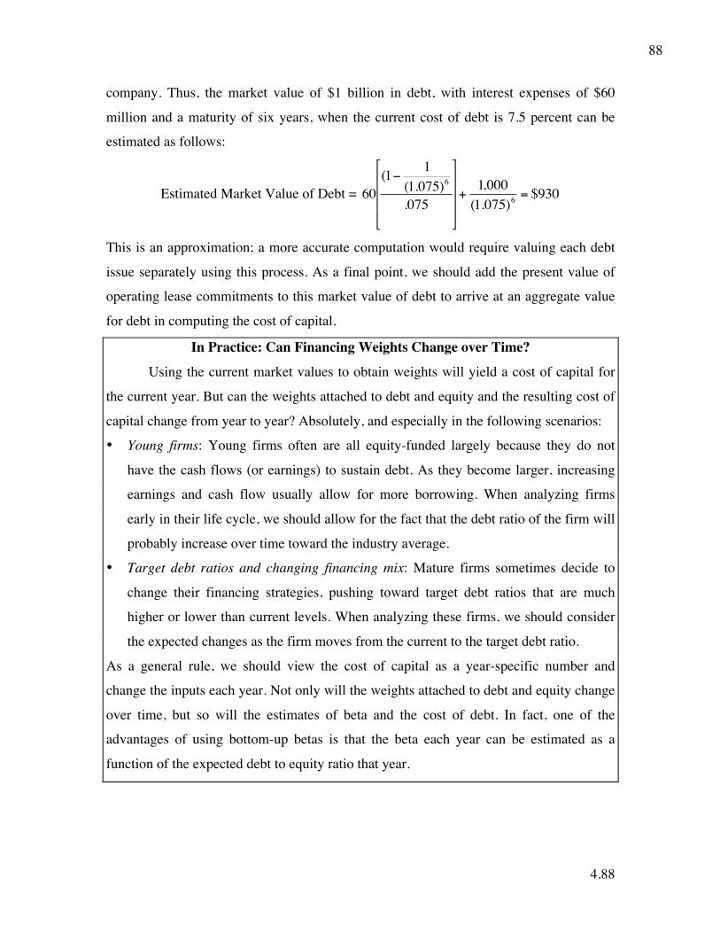
4.88

88

company. Thus, the market value of $1 billion in debt, with interest expenses of $60

million and a maturity of six years, when the current cost of debt is 7.5 percent can be

estimated as follows:

Estimated Market Value of Debt =

€

60(1− 1

(1.075)6

.075

⎡

⎣

⎢ ⎢ ⎢

⎤

⎦

⎥ ⎥ ⎥

+1,000(1.075)6

= $930

This is an approximation; a more accurate computation would require valuing each debt

issue separately using this process. As a final point, we should add the present value of

operating lease commitments to this market value of debt to arrive at an aggregate value

for debt in computing the cost of capital.

In Practice: Can Financing Weights Change over Time?

Using the current market values to obtain weights will yield a cost of capital for

the current year. But can the weights attached to debt and equity and the resulting cost of

capital change from year to year? Absolutely, and especially in the following scenarios:

• Young firms: Young firms often are all equity-funded largely because they do not

have the cash flows (or earnings) to sustain debt. As they become larger, increasing

earnings and cash flow usually allow for more borrowing. When analyzing firms

early in their life cycle, we should allow for the fact that the debt ratio of the firm will

probably increase over time toward the industry average.

• Target debt ratios and changing financing mix: Mature firms sometimes decide to

change their financing strategies, pushing toward target debt ratios that are much

higher or lower than current levels. When analyzing these firms, we should consider

the expected changes as the firm moves from the current to the target debt ratio.

As a general rule, we should view the cost of capital as a year-specific number and

change the inputs each year. Not only will the weights attached to debt and equity change

over time, but so will the estimates of beta and the cost of debt. In fact, one of the

advantages of using bottom-up betas is that the beta each year can be estimated as a

function of the expected debt to equity ratio that year.

4.89

89

Illustration 4.17: Market Value and Book Value Debt Ratios: Disney and Aracruz

Disney has a number of debt issues on its books, with varying coupon rates and

maturities. Table 4.28 summarizes Disney’s outstanding debt, broken down by when the

debt comes due; we treat the debt due in 2009 as due in 1 year, the debt due in 2010 as

due in 2 years and so on. The debt due after 2013 is given a maturity of 10 years, based

upon a perusal of the actual due dates on the long term debt.

Table 4.28 Debt at Disney: May 2009

Due in Maturity Amount due % due 2009 1 $3,513 24.33% 2010 2 $1,074 7.44% 2011 3 $1,205 8.35% 2012 4 $1,479 10.24% 2013 5 $1,842 12.76%

Thereafter 10 $5,324 36.88% Weighted Average 5.38 years $14,437

To convert the book value of debt to market value, we use the current pretax cost of debt

for Disney of 6 percent as the discount rate, the face value of debt ($16,003 million) in

May 2009 as the book value of debt and the current year’s interest expenses of $728

million as the coupon payment:

Estimated MV of Disney Debt =

€

728(1− 1

(1.06)5.38

.06

⎡

⎣

⎢ ⎢ ⎢

⎤

⎦

⎥ ⎥ ⎥ +

16,003(1.06)5.38 = $14,962 million

To this amount, we add the present value of Disney’s operating lease commitments. This

present value is computed by discounting the lease commitment each year at the pretax

cost of debt for Disney (6 percent) in table 4.29:55

Table 4.29: Present Value of Operating Leases at Disney

Year Commitment (in millions) Present Value (in millions) 1 $392.00 $369.81 2 $351.00 $312.39

3 $305.00 $256.08

55Disney reports total commitments of $715 million beyond year six. Using the average commitment from years one through five as an indicator, we assumed that this total commitment would take the form of an annuity of $178.75 million a year for four years.

4.90

90

4 $265.00 $209.90 5 $198.00 $147.96

6–7 $309.50 $424.02 Debt value of leases = $1,720.17

Adding the debt value of operating leases to the market value of debt of $14,962 million

yields a total market value for debt of $ 16,682 million at Disney.

For Aracruz and Tata Chemicals, we use the book value of debt as a proxy for the

market value of debt. For the former, this is because a significant portion of its debt is

recent (and should therefore reflect current market interest rates and prices.). For the

latter, a large portion of the debt is short term, which should ensure that the market value

and book value of debt will converge. In Table 4.30 we contrast the book value debt

ratios with the market value debt ratios for Disney, Aracruz and Tata Chemicals. The

market value of equity is estimated using the current market price and the number of

shares outstanding.

Table 4.30 Book Value versus Market Value: Debt Ratios

Company Book D/E Book Debt/Capital Market D/E

Market Debt/Capital

Disney 49.01% 32.89% 36.91% 26.96% Aracruz 1012.22% 91.01% 110.41% 52.47% Tata Chemicals 75.83% 43.13% 51.56% 34.02%

For Disney, the market value debt ratio of 26.96% percent is lower than the book value

debt ratio of 32.89 percent. That pattern is repeated for Aracruz and Tata Chemicals, with

the difference being largest at Aracuz, where book value of equity recorded a significant

write-down in 2008 (as a result of their trading losses in derivatives).

Estimating and Using the Cost of Capital

With the estimates of the costs of the individual components—debt, equity and

preferred stock (if any)—and the market value weights of each of the components, the

cost of capital can be computed. Thus if E, D, and PS are the market values of equity,

debt, and preferred stock respectively, the cost of capital can be written as follows:

Cost of Capital = kE [E/(D + E + PS)] + kD[D/(D + E + PS)] + kPS [PS/(D + E + PS)]

The cost of capital is a measure of the composite cost of raising money that a firm faces.

It will generally be lower than the cost of equity, which is the cost of just equity funding.

4.91

91

It is a source of confusion to many analysts that both the cost of equity and the

cost of capital are used as hurdle rates in investment analysis. The way to resolve this

confusion is to recognize when it is appropriate to use each one.

• If we want to adopt the perspective of just the equity investors in a business or a

project and measure the returns earned just by these investors on their investment,

the cost of equity is the correct hurdle rate to use. In measuring the returns to

equity investors then, we have to consider only the income or cash flows left over

after all other claimholders needs (interest payments on debt and preferred

dividends, for instance) have been met.

• If the returns that we are measuring are composite returns to all claimholders,

based on earnings before payments to debt and preferred stockholders, the

comparison should be to the cost of capital.

Although these principles are abstract, we will consider them in more detail in the next

chapter when we look at examples of projects.

wacc.xls: This data set online has the average cost of capital, by industry (sector),

for the United States.

Hurdle Rates: A Behavioral Perspective

Our discussion of cost of equity and capital has centered on a critical premise that

the right hurdle rate for a firm should reflect the weighted average of the cost of financing

the firm today. As a consequence, we used the current costs of debt and equity, updated

to reflect today’s riskfree rates and risk premiums, and weighted them based upon market

values. But do managers subscribe to this approach? There is substantial evidence that

some of them do not and the reasons may have more to do with behavioral considerations

than financial arguments. Surveys of how firms set hurdle rates for investments indicate

the following:

a. Book value versus Market value: Many firms continue to use book values for debt

and equity to compute weights, rather than market values. One reason, stated or

unstated, for this practice is that book debt ratios are more stable than market debt

4.92

92

ratios. This is almost a given since the market values (at least of equity) change

continuously but the book values do not change until the next financial statement is

put together. Intellectually, we can argue (as we have) that the stability of debt ratios

is an illusion, but it is human nature to prefer stability to volatility.

b. Outsourcing risk premiums and betas: In the earlier parts of this chapter, we noted

that it is common practice for firms to purchase estimates of equity risk premiums and

betas for external sources, Ibbotson Associates for the former and Barra for the latter.

While we believe that it is dangerous to outsource key components of the cost of

capital to an outside source, it makes sense from a behavioral standpoint. Using

external sources for data gives managers someone else to blame, if things go wrong,

and thus deflects any criticism that they may have faced for bad decisions.

c. Hurdle rate not equal to cost of capital: In many firms, the hurdle rate that is used for

assessing investments is not based upon the cost of capital. Instead, it is set at a value

above or below the cost of capital and often reflects what the firm has earned on

projects it has invested in the past.56 Thus, a firm that has generated a 15% return on

capital on past investments will use a hurdle rate of 15% for future investments,

rather than its computed cost of capital. From a behavioral finance perspective, this

practice does make sense since it reflects both anchoring (where managers start with

the familiar, i.e., past returns, as their anchors for estimates) and availability biases

(where they overweight recent project return experience too much).

So, how should managers set hurdle rates in a world that is composed of irrational

investors? In a paper examining this question, Stein argues that firms that are focused on

long term value maximization should continue to use the conventional cost of capital as

the hurdle rate, with the proviso that betas reflect the true economic risk of the enterprise

rather than returns over short time periods. However, if the objective is to maximize the

current stock price, the hurdle rate used should not be the cost of capital but should be

adjusted for whatever errors investors are making in assessing stock price; he suggests

56 Driver, C. and P. Temple, 2009, Why do hurdle rates differ from the cost of capital? Cambridge Journal of Economics, 1-23. They compare the costs of capital and hurdle rates for 3000 business units at 450 companies that are part of the PIMS database and find that while 1425 units use hurdle rates that are roughly equal to their costs of capital, 505 units use hurdle rates less than the cost of capital and 452 use hurdle rates that are higher than their costs of capital.

4.93

93

using the price to book ratio as a proxy for this adjustment. This can lead to hurdle rates

being lower than the cost of capital for some firms and higher for others.57

Illustration 4.18: Estimating Cost of Capital

Culminating the analysis in this chapter, we first estimate the costs of capital for

each of Disney’s divisions. In making these estimates, we use the costs of equity that we

obtained for the divisions in Illustration 4.13 and Disney’s cost of debt from Illustration

4.14. We also assume that all of the divisions are funded with the same mix of debt and

equity as the parent company. Table 4.31 provides estimates of the costs of capital for the

divisions:

Table 4.31 Cost of Capital for Disney’s Divisions

Business Cost of Equity After-tax cost

of debt E/(D+E) D/(D+E) Cost of capital Media Networks 8.61% 3.72% 75.00% 25.00% 7.39% Parks and Resorts 8.20% 3.72% 64.68% 35.32% 6.62% Studio Entertainment 13.53% 3.72% 68.64% 31.36% 10.45% Consumer Products 10.86% 3.72% 80.84% 19.16% 9.49% Disney 8.91% 3.72% 73.04% 26.96% 7.51%

The cost of capital for Disney’s operating assets is 7.51 percent, but the costs of capital

vary across divisions with a low of 6.62 percent for the parks and resorts division to a

high or 10.45 percent for studio entertainment.

To estimate the cost of capital in U.S. dollars for Aracruz, we use the cost of

equity of 20.82%,(from Illustration 4.13), the after-tax cost of debt of 5.61% (from

Illustration 4.14) and the debt to capital ratio of 52.47% (estimated based upon the

current market values of debt and equity):

Cost of capital$ = 20.82% (1-0.5247) + 5.61% (0.5247) = 12.84%

This dollar cost of capital can be converted into nominal $R cost of capital or a real cost

of capital, by adjusting for inflation:

Cost of capitalR$ = (1+ Cost of capital$)

€

(1+ Expected InflationR$)(1+ Expected InflationUS $)

−1

57 Stein,  J.,  1996,  ‘Rational  capital  budgeting  in  an  irrational  world’,  Journal  of  Business,  Vol.  69,  pp.  429–55.  

4.94

94

= 1.1284

€

(1.07)(1.02)

−1=18.37%

Cost of capitalReak = (1+ Cost of capital$)

€

1(1+ Expected InflationUS $)

−1

= 1.1284

€

1(1.02)

−1=10.63%

Note again that the only reason for the differences across the estimates of cost of capital

is different expectations for inflation: 0% for real, 2% for US dollars and 7% for $R.

To estimate the cost of capital for Tata Chemicals, we look at its two businesses –

fertilizers and chemicals – and use the estimates of cost of equity and debt obtained in

earlier illustrations. Table 4.32 summarizes the estimates:

Table 4.32: Cost of capital- Tata Chemicals

Business Cost of equity

Pre-tax cost of debt

After-tax cost of debt

D/(D+E) Cost of capital

Fertilizers 14.14% 10.0% 6.60% 34.02% 11.58% Chemicals 13.58% 10.0% 6.60% 34.02% 11.21% Tata Chemicals

13.93% 10.0% 6.60% 34.02% 11.44%

We stayed with the assumption that we made earlier that the debt ratios of the two

divisions would the same as the overall company.

When estimating the cost of equity for Bookscape, we assumed that the company

would be funded using the same market debt to equity ratio as the book/publishing

industry. Staying consistent, we will use the market debt to capital ratio of the sector to

compute the cost of capital for the firm. We will also present two estimates of the cost of

capital—one using the market beta and the other using the total beta – in table 4.33:

Table 4.33: Cost of capital for Bookscape- Market and Total Beta

Cost of equity

Pre-tax Cost of debt

After-tax cost of debt D/(D+E)

Cost of capital

Market Beta 11.60% 6.00% 3.60% 34.84% 8.81% Total Beta 20.94% 6.00% 3.60% 34.84% 14.90%

4.95

95

The cost of capital estimated using the total beta is a more realistic estimate, given that

this is a private company, and we will use it as the cost of capital for Bookscape in the

coming chapters.

In Practice: Equity, Debt, and Cost of Capital for Banks

Note that we did not estimate a cost of capital for Deutsche Bank even though we

have estimates of the costs of equity and debt for the firm. The reason is simple and goes

to the heart of how firms view debt. For nonfinancial service firms, debt is a source of

capital and is used to fund real projects—building a factory or making a movie. For

banks, debt is raw material that is used to generate profits. Boiled down to its simplest

elements, it is a bank’s job to borrow money (debt) at a low rate and lend it out at a

higher rate. It should come as no surprise that when banks (and their regulators) talk

about capital, they mean equity capital.58

There is also a practical problem in computing the cost of capital for a bank. If we

define debt as any fixed commitment where failure to meet the commitment can lead to

loss of equity control, the deposits made by customers at bank branches would qualify

and the debt ratio of a bank will very quickly converge on 100 percent. If we define it

more narrowly, we still are faced with a problem of where to draw the line. A pragmatic

compromise is to view only long-term bonds issued by a bank as debt, but it is an

artificial one. Deutsche Bank, for instance, had long-term debt in December 2008 with a

value of 143 billion Euros and common equity with a market value of 30 billion Euros.

Using the cost of equity of 10.55 percent (from Illustration 4.13) and the after-tax cost of

debt of 3.13 percent (from Illustration 4.14), we obtain a cost of capital:

Cost of capital = 10.55% (30/173) + 4.12%(143/173)

= 5.23%

However, this number is tainted by the arbitrary definition of debt as only long term debt.

With Deutsche Bank, we will do almost all of our analyses using the cost of equity rather

than the cost of capital.

58All of the capital ratios that govern banks are stated in terms of book value of equity, though equity is defined broadly to include preferred stock.

4.96

96

Conclusion This chapter explains the process of estimating discount rates, by relating them to

the risk and return models described in the previous chapter:

• The cost of equity can be estimated using risk and return models—the CAPM, where

risk is measured relative to a single market factor; the APM, where the cost of equity

is determined by the sensitivity to multiple unspecified economic factors; or a

multifactor model, where sensitivity to macroeconomic variables is used to measure

risk.

• In both these models, the key inputs are the risk-free rate, the risk premiums,

and the beta (in the CAPM) or betas (in the APM). The last of these inputs is

usually estimated using historical data on prices.

• Although the betas are estimated using historical data, they are determined by

the fundamental decisions that a firm makes on its business mix, operating,

and financial leverage. Consequently, we can get much better estimates of

betas by looking at sector averages and correcting for differences across firms.

• The cost of capital is a weighted average of the costs of the different components of

financing, with the weights based on the market values of each component. The cost

of debt is the market rate at which the firm can borrow long term, adjusted for any tax

advantages of borrowing. The cost of preferred stock, on the other hand, is the

preferred dividend.

• The cost of capital is the minimum acceptable hurdle rate that will be used to

determine whether to invest in a project.

While we will use the cost of capital as our hurdle rate, when assessing investments, in

the next two chapters, we are also aware that many firms use hurdle rates that are

different from their costs of capital.

4.97

97

Live Case Study

Risk and Return: Analysis for the Firm Objective: To develop a risk profile for your company, estimate its risk parameters and

use these parameters to estimate costs of equity and capital for the firm.

Key Questions:

• What is the risk profile of your company? (How much overall risk is there in this

firm? Where is this risk coming from (market, firm, industry or currency)? How is

the risk profile changing?)

• What is the performance profile of an investment in this company? What return

would you have earned investing in this company’s stock? Would you have under or

out performed the market? How much of the performance can be attributed to

management?

• How risky is this company’s equity? Why? What is its cost of equity?

• How risky is this company’s debt? What is its cost of debt?

• What is the mix of debt and equity used by this firm to fund its investments?

• What is this company’s current cost of capital?

Framework for Analysis:

1. Estimating Historical Risk Parameters (Top Down Betas)

Run a regression of returns on your firm’s stock against returns on a market

index, preferably using monthly data and 5 years of observations (or)

• What is the intercept of the regression? What does it tell you about the

performance of this company’s stock during the period of the regression?

• What is the slope of the regression?

• What does it tell you about the risk of the stock?

• How precise is this estimate of risk? (Provide a range for the estimate.)

• What portion of this firm’s risk can be attributed to market factors? What

portion to firm-specific factors? Why is this important?

• How much of the “risk” for this firm is due to business factors? How much of

it is due to financial leverage?

2. Comparing to Sector Betas (Bottom up Betas)

4.98

98

• Break down your firm by business components, and estimate a business beta

for each component

• Attach reasonable weights to each component and estimate a unlevered beta

for the business.

• Using the current leverage of the company, estimate a levered beta for each

component.

3. Choosing Between Betas

• Which of the betas that you have estimated for the firm (top down or bottom

up) would you view as more reliable? Why?

• Using the beta that you have chosen, estimate the expected return on an equity

investment in this company to equity investors in the company?

• As a manager in this firm, how would you use this expected return?

4. Estimating Default Risk and Cost of Debt

• If your company is rated,

• What is the most recent rating for the firm?

• What is the default spread and interest rate associated with this rating?

• If your company has bonds outstanding, estimate the yield to maturity

on a long term bond? Why might this be different from the rate

estimated in the last step?

• What is the company’s marginal tax rate?

• If your company is not rated,

• Does it have any recent borrowings? If yes, what interest rate did the

company pay on these borrowing?

• Can you estimate a “synthetic” rating? If yes, what interest rate would

correspond to this rating?)

5. Estimating Cost of Capital

• Weights for Debt and Equity

• What is the market value of equity?

• Estimate a market value for debt. (To do this you might have to collect

information on the average maturity of the debt, the interest expenses

in the most recent period and the book value of the debt)

4.99

99

• What are the weights of debt and equity?

• Cost of Capital

• What is the cost of capital for the firm?

Getting Information on Risk and Return

If you want to run a regression of stock returns against a market index to estimate

a beta, you will need to estimate past returns for both the stock and index. Several data

services provide access to the data. If you want a beta estimate for your firm, you can

find it online or obtain it from a data service. If you want to estimate bottom-up betas,

based upon comparable firms, you will first have to identify the businesses that your firm

operates in (which should be available in the firm’s 10-K), find comparable firms in each

business and then estimate the average beta and debt to equity ratio for these firms.

You can find the rating for your company from the S&P and Moody publications

that list all traded bonds and their ratings. Alternatively, you can estimate an interest

coverage ratio and a synthetic rating.

Online sources of information:

http://www.stern.nyu.edu/~adamodar/cfin2E/project/data.htm

4.100

100

Problems and Questions

In the problems below, use 5.5% as your market risk premium where none is specified.

1. In December 1995, Boise Cascade’s stock had a beta of 0.95. The Treasury bill rate at the time

was 5.8 percent, and the Treasury bond rate was 6.4 percent. The firm had debt outstanding of

$1.7 billion and a market value of equity of $1.5 billion; the corporate marginal tax rate was 36

percent.

a. Estimate the expected return on the stock for a short-term investor in the company.

b. Estimate the expected return on the stock for a long-term investor in the company.

c. Estimate the cost of equity for the company.

2. Boise Cascade also had debt outstanding of $1.7 billion and a market value of equity of $1.5

billion; the corporate marginal tax rate was 36 percent. <AQ: Question 2 is a repeat of the info

for question 1. Couldn't parts a and be become d and e of question 1 instead? No new

information introduced here. Leave as is>

a. Assuming that the current beta of 0.95 for the stock is a reasonable one, estimate the unlevered

beta for the company.

b. How much of the risk in the company can be attributed to business risk and how much to

financial leverage risk?

3. Biogen, a biotechnology firm, had a beta of 1.70 in 1995. It had no debt outstanding at the end

of that year.

a. Estimate the cost of equity for Biogen, if the Treasury bond rate is 6.4 percent.

b. What effect will an increase in long-term bond rates to 7.5 percent have on Biogen’s cost of

equity?

c. How much of Biogen’s risk can be attributed to business risk?

4. Genting Berhad is a Malaysian conglomerate with holdings in plantations and tourist resorts.

The beta estimated for the firm, relative to the Malaysian stock exchange, is 1.15, and the long-

term government borrowing rate in Malaysia is 11.5 percent.

a. Estimate the expected return on the stock.

b. If you were an international investor, what concerns (if any) would you have about using the

beta estimated relative to the Malaysian index? If you do, how would you modify the beta?

4.101

101

5. You have just done a regression of monthly stock returns of HeavyTech, a manufacturer of

heavy machinery, on monthly market returns over the past five years and come up with the

following regression:

RHeavyTech = 0.5% + 1.2RM The variance of the stock is 50 percent, and the variance of the market is 20 percent. The current

Treasure bill rate is 3 percent (it was 5 percent one year ago). The stock is currently selling for

$50, down $4 over the past year, and has paid a dividend of $2 during the past year and expects

to pay a dividend of $2.50 over the next year. The NYSE composite has gone down 8 percent

over the past year, with a dividend yield of 3 percent. HeavyTech has a tax rate of 40 percent.

a. What is the expected return on HeavyTech over the next year?

b. What would you expect HeavyTech’s price to be one year from today?

c. What would you have expected HeavyTech’s stock returns to be over the past year?

d. What were the actual returns on HeavyTech over the past year?

e. HeavyTech has $100 million in equity and $50 million in debt. It plans to issue $50 million

in new equity and retire $50 million in debt. Estimate the new beta.

6. Safecorp, which owns and operates grocery stores across the United States, currently has $50

million in debt and $100 million in equity outstanding. Its stock has a beta of 1.2. It is planning a

leveraged buyout, where it will increase its debt/equity ratio of 8. If the tax rate is 40 percent,

what will the beta of the equity in the firm be after the leveraged buyout?

7. Novell, which had a market value of equity of $2 billion and a beta of 1.50, announced that it

was acquiring WordPerfect, which had a market value of equity of $1 billion and a beta of 1.30.

Neither firm had any debt in its financial structure at the time of the acquisition, and the

corporate tax rate was 40 percent.

a. Estimate the beta for Novell after the acquisition, assuming that the entire acquisition was

financed with equity.

b. Assume that Novell had to borrow the $1 billion to acquire WordPerfect. Estimate the beta

after the acquisition.

8. You are analyzing the beta for Hewlett Packard and have broken down the company into four

broad business groups, with market values and betas for each group.

Business Group Market Value of Equity Beta

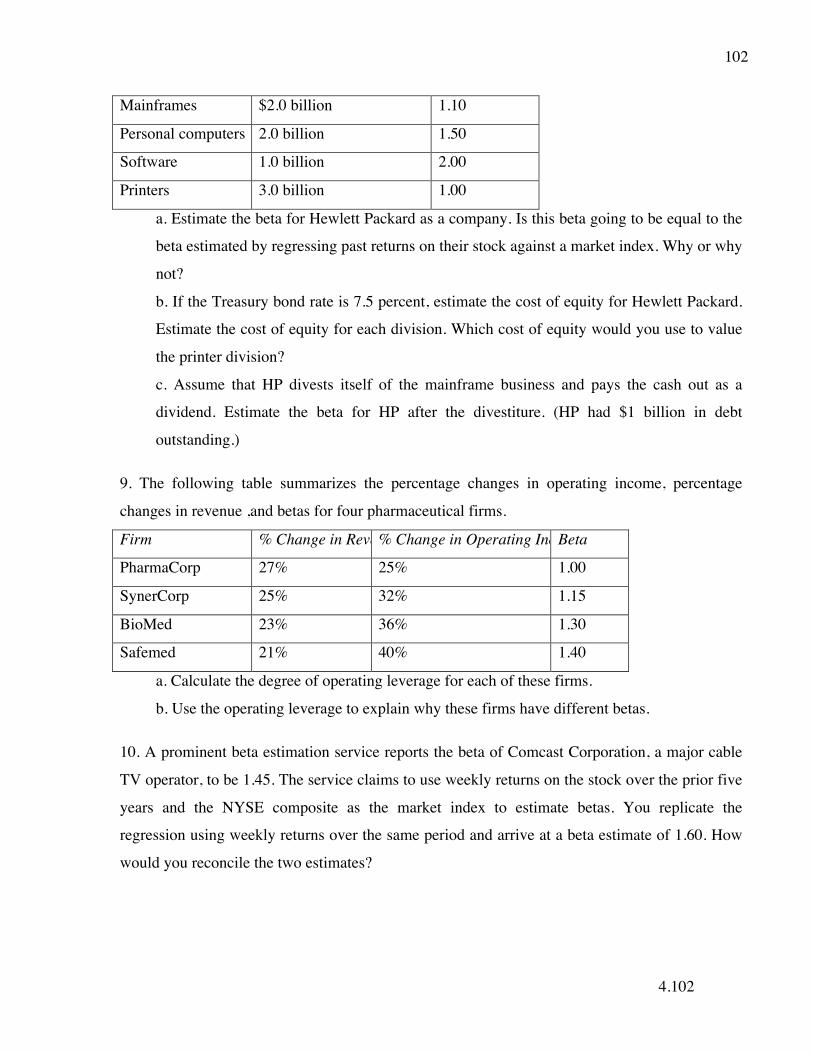
4.102

102

Mainframes $2.0 billion 1.10

Personal computers 2.0 billion 1.50

Software 1.0 billion 2.00

Printers 3.0 billion 1.00

a. Estimate the beta for Hewlett Packard as a company. Is this beta going to be equal to the

beta estimated by regressing past returns on their stock against a market index. Why or why

not?

b. If the Treasury bond rate is 7.5 percent, estimate the cost of equity for Hewlett Packard.

Estimate the cost of equity for each division. Which cost of equity would you use to value

the printer division?

c. Assume that HP divests itself of the mainframe business and pays the cash out as a

dividend. Estimate the beta for HP after the divestiture. (HP had $1 billion in debt

outstanding.)

9. The following table summarizes the percentage changes in operating income, percentage

changes in revenue ,and betas for four pharmaceutical firms.

Firm % Change in Revenue % Change in Operating Income Beta

PharmaCorp 27% 25% 1.00

SynerCorp 25% 32% 1.15

BioMed 23% 36% 1.30

Safemed 21% 40% 1.40

a. Calculate the degree of operating leverage for each of these firms.

b. Use the operating leverage to explain why these firms have different betas.

10. A prominent beta estimation service reports the beta of Comcast Corporation, a major cable

TV operator, to be 1.45. The service claims to use weekly returns on the stock over the prior five

years and the NYSE composite as the market index to estimate betas. You replicate the

regression using weekly returns over the same period and arrive at a beta estimate of 1.60. How

would you reconcile the two estimates?

4.103

103

11. Battle Mountain is a mining company that mines gold, silver, and copper in mines in South

America, Africa, and Australia. The beta for the stock is estimated to be 0.30. Given the

volatility in commodity prices, how would you explain the low beta?

12. You have collected returns on AnaDone , a large diversified manufacturing firm, and

the NYSE index for five years:

Year Returns (%)

for AnaDone

Returns (%)

for NYSE

1981 10% 5%

1982 5% 15%

1983 –5% 8%

1984 20% 12%

1985 –5% –5%

a. Estimate the intercept (alpha) and slope (beta) of the regression.

b. If you bought stock in AnaDone today, how much would you expect to make as a

return over the next year? (The six-month Treasure bill rate is 6 percent.)

c. Looking back over the past five years, how would you evaluate AnaDone’s

performance relative to the market?

d. Assume now that you are an undiversified investor and that you have all of your

money invested in AnaDone. What would be a good measure of the risk that you are

taking on? How much of this risk would you be able to eliminate if you diversify?

e. AnaDone is planning to sell off one of its divisions. The division under consideration

has assets which comprise half of the book value of AnaDone and 20 percent of the

market value. Its beta is twice the average beta for AnaDone (before divestment).

What will the beta of AnaDone be after divesting this division?

13. You run a regression of monthly returns of Mapco, an oil- and gas-producing firm, on the

S&P 500 Index and come up with the following output for the period 1991 to 1995.

Intercept of the regression = 0.06%

X-coefficient of the regression = 0.46

Standard error of X-coefficient = 0.20

R2 = 5%

4.104

104

There are 20 million shares outstanding, and the current market price is $2/share. The firm has

$20 million in debt outstanding. (The firm has a tax rate of 36 percent.)

a. What would an investor in Mapco’s stock require as a return, if the Treasure bond rate is

6 percent?

b. What proportion of this firm’s risk is diversifiable?

c. Assume now that Mapco has three divisions, of equal size (in market value terms). It

plans to divest itself of one of the divisions for $20 million in cash and acquire another

for $50 million (it will borrow $30 million to complete this acquisition). The division it is

divesting is in a business line where the average unlevered beta is 0.20, and the division it

is acquiring is in a business line where the average unlevered beta is 0.80. What will the

beta of Mapco be after this acquisition?

14. You have just run a regression of monthly returns of American Airlines (AMR) against the

S&P 500 over the past five years. You have misplaced some of the output and are trying to

derive it from what you have.

a. You know the R2 of the regression is 0.36, and that your stock has a variance of 67 percent. The market variance is 12 percent . What is the beta of AMR?

b. You also remember that AMR was not a very good investment during the period of the

regression and that it did worse than expected (after adjusting for risk) by 0.39 percent a

month for the five years of the regression. During this period, the average risk-free rate

was 4.84 percent. What was the intercept on the regression?

c. You are comparing AMR to another firm that also has an R2 of 0.48. Will the two firms

have the same beta? If not, why not?

15. You have run a regression of monthly returns on Amgen, a large biotechnology firm, against

monthly returns on the S&P 500 Index, and come up with the following output:

Rstock = 3.28% + 1.65 RMarket R2 = 0.20

The current one-year Treasury bill rate is 4.8 percent and the current thirty-year bond rate is 6.4

percent. The firm has 265 million shares outstanding, selling for $30 per share. a. What is the expected return on this stock over the next year?

b. Would your expected return estimate change if the purpose was to get a discount rate to

analyze a thirty-year capital budgeting project?

4.105

105

c. An analyst has estimated correctly that the stock did 51.10 percent better than expected

annually during the period of the regression. Can you estimate the annualized risk-free

rate that she used for her estimate?

d. The firm has a debt/equity ratio of 3 percent and faces a tax rate of 40 percent. It is planning to

issue $2 billion in new debt and acquire a new business for that amount, with the same risk level

as the firm’s existing business. What will the beta be after the acquisition?

16. You have just run a regression of monthly returns on MAD, a newspaper and

magazine publisher, against returns on the S&P 500, and arrived at the following result:

RMAD = – 0.05% + 1.20 RS&P

The regression has an R2 of 22 percent. The current Treasure bill rate is 5.5 percent and

the current Treasure bond rate is 6.5 percent. The risk-free rate during the period of the

regression was 6 percent. Answer the following questions relating to the regression:

a. Based on the intercept, you can conclude that the stock did

i. 0.05 percent worse than expected on a monthly basis, during the regression.

ii. 0.05 percent better than expected on a monthly basis during the period of the

regression.

iii. 1.25 percent better than expected on a monthly basis during the period of the

regression.

iv. 1.25 percent worse than expected on a monthly basis during the period of the

regression.

v. None of the above.

b. You now realize that MAD went through a major restructuring at the end of last

month (which was the last month of your regression), and made the following

changes:

• The firm sold off its magazine division, which had an unlevered beta of 0.6, for

$20 million.

• It borrowed an additional $20 million, and bought back stock worth $40 million.

After the sale of the division and the share repurchase, MAD had $40 million in debt and

$120 million in equity outstanding. If the firm’s tax rate is 40 percent, reestimate the beta

after these changes.

4.106

106

17. Time Warner, the entertainment conglomerate, has a beta of 1.61. Part of the reason for the

high beta is the debt left over from the leveraged buyout of Time by Warner in 1989, which

amounted to $10 billion in 1995. The market value of equity at Time Warner in 1995 was also

$10 billion. The marginal tax rate was 40 percent.

a. Estimate the unlevered beta for Time Warner.

b. Estimate the effect of reducing the debt ratio by 10 percent each year for the next two

years on the beta of the stock.

18. Chrysler, the automotive manufacturer, had a beta of 1.05 in 1995. It had $13 billion in debt

outstanding in that year and 355 million shares trading at $50 per share. The firm had a cash

balance of $8 billion at the end of 1995. The marginal tax rate was 36 percent.

a. Estimate the unlevered beta of the firm.

b. Estimate the effect of paying out a special dividend of $5 billion on this unlevered beta.

c. Estimate the beta for Chrysler after the special dividend.

19. You are trying to estimate the beta of a private firm that manufactures home appliances. You

have managed to obtain betas for publicly traded firms that also manufacture home appliances.

Firm Beta Debt (in millions) MV of Equity (in

millions)

Black & Decker 1.40 $2,500 $ 3,000

Fedders Corp. 1.20 $ 5 $ 200

Maytag Corp. 1.20 $ 540 $ 2250

National Presto 0.70 $ 8 $ 300

Whirlpool 1.50 $ 2900 $ 4000

The private firm has a debt equity ratio of 25 percent and faces a tax rate of 40 percent. The

publicly traded firms all have marginal tax rates of 40 percent, as well.

a. Estimate the beta for the private firm.

b. What concerns, if any, would you have about using betas of comparable firms?

20. As the result of stockholder pressure, RJR Nabisco is considering spinning off its food

division. You have been asked to estimate the beta for the division and decide to do so by

obtaining the beta of comparable publicly traded firms. The average beta of comparable publicly

4.107

107

traded firms is 0.95, and the average debt/equity ratio of these firms is 35 percent. The division is

expected to have a debt ratio of 25 percent. The marginal corporate tax rate is 36 percent.

a. What is the beta for the division?

b. Would it make any difference if you knew that RJR Nabisco had a much higher fixed

cost structure than the comparable firms used here?

21. Southwestern Bell, a phone company, is considering expanding its operations into the media

business. The beta for the company at the end of 1995 was 0.90, and the debt/equity ratio was 1.

The media business is expected to be 30 percent of the overall firm value in 1999, and the

average beta of comparable firms is 1.20; the average debt/equity ratio for these firms is 50

percent. The marginal corporate tax rate is 36 percent. <AQ: Should the dates in this question be

updated?>

a. Estimate the beta for Southwestern Bell in 1999, assuming that it maintains its current

debt/equity ratio.

b. Estimate the beta for Southwestern Bell in 1999, assuming that it decides to finance its

media operations with a debt/equity ratio of 50 percent.

22. The chief financial officer of Adobe Systems, a software manufacturing firm, has approached

you for some advice regarding the beta of his company. He subscribes to a service that estimates

Adobe System’s beta each year, and he has noticed that the beta estimates have gone down every

year since 1991—2.35 in 1991 to 1.40 in 1995. He would like the answers to the following

questions

a. Is this decline in beta unusual for a growing firm?

b. Why would the beta decline over time?

c. Is the beta likely to keep decreasing over time?

23. You are analyzing Tiffany’s, an upscale retailer, and find that the regression estimate of the

firm’s beta is 0.75; the standard error for the beta estimate is 0.50. You also note that the average

unlevered beta of comparable specialty retailing firms is 1.15.

a. If Tiffany’s has a debt/equity ratio of 20 percent, estimate the beta for the company

based on comparable firms. (The tax rate is 40 percent)

b. Estimate a range for the beta from the regression.

4.108

108

c. How would you reconcile the two estimates? Which one would you use in your analysis?