Applications of the Proper Orthogonal Decomposition Methodcfdbib/repository/WN_CFD_07_97.pdf ·...

Applications of the Proper Orthogonal DecompositionMethod

Internship report

Katrin GRAUMentoring: Laurent GICQUEL

September 2007

WN/CFD/07/97

I would like to thank the whole CFD team at CERFACS, in particular

− L. Gicquel, my supervisor, for his excellent mentoring and support,

− A. Roux, who explained his codes to me and helped me with all the occuring problems,

− M. Leyko, for providing me the snapshots for the applications and discussing the results,

− T. Poinsot, for the opportunity to do an internship in the CFD team at CERFACS.

Contents

1 Introduction 2

2 Proper Orthogonal Decomposition Method 2

3 Application: “Perfect” Square 4

3.1 Theory . . . . . . . . . . . . . . . . . . . . . . . . . . . . . . . . . . . . . . . . . . 4

3.2 AVBP . . . . . . . . . . . . . . . . . . . . . . . . . . . . . . . . . . . . . . . . . . 6

3.3 Proper Orthogonal Decomposition . . . . . . . . . . . . . . . . . . . . . . . . . . 6

3.3.1 Pressure fluctuation . . . . . . . . . . . . . . . . . . . . . . . . . . . . . . 7

3.3.2 Velocity fluctuation . . . . . . . . . . . . . . . . . . . . . . . . . . . . . . 8

3.3.3 Pressure and velocity fluctuation . . . . . . . . . . . . . . . . . . . . . . . 10

3.4 Conclusions . . . . . . . . . . . . . . . . . . . . . . . . . . . . . . . . . . . . . . . 13

4 Application: Square 13

4.1 AVBP . . . . . . . . . . . . . . . . . . . . . . . . . . . . . . . . . . . . . . . . . . 13


4.3 Conclusions . . . . . . . . . . . . . . . . . . . . . . . . . . . . . . . . . . . . . . . 18

5 Application: Square, 3 initial modes 19

5.1 AVBP . . . . . . . . . . . . . . . . . . . . . . . . . . . . . . . . . . . . . . . . . . 19


5.3 Conclusions . . . . . . . . . . . . . . . . . . . . . . . . . . . . . . . . . . . . . . . 21

6 Application: L-Shape 23

6.1 AVBP . . . . . . . . . . . . . . . . . . . . . . . . . . . . . . . . . . . . . . . . . . 23


6.3 Conclusions . . . . . . . . . . . . . . . . . . . . . . . . . . . . . . . . . . . . . . . 26

7 Conclusions 26

Annex 29

1

1 Introduction

With the increase of the capacity of computers used for numerical simulations the amount ofproduced data has increased as well. These large amounts of data have to be analyzed to gaina better understanding of the simulated processes.The Proper Orthogonal Decomposition (POD) is a post-processing technique. It takes a givenset of data and extracts basis functions, that contain as much “energy” as possible. The meaningof “energy” depends on which kind of POD is used.One problem that occurs is the choice of variables that should be taken into account whileusing POD. If the numerical simulation is made for incompressible flows, only the velocity is avariable of interest. In a compressible flow, the pressure becomes important as well and shouldbe included when performing POD.

The object of this internship was to test the existing POD tool at CERFACS using differentacademic applications to investigate the effect of the chosen inner product.

2 Proper Orthogonal Decomposition Method

An overview over the POD method can be found for example in [4], but a short summary of theparts of POD relevant for the following applications is given here (see [1], [2], [3], [4], [5], [6],[10]).

Let qk(x), k = 1 . . . Nt, be a set of observations (called “snapshots”) at points x ∈ Ω, that couldbe obtained by a numerical simulation or experimental measurements. The goal of POD is tofind functions φ such that

〈|(q, φ)|2〉‖φ‖2

(1)

is maximized. 〈.〉 is some kind of average, (., .) is an inner product and ‖.‖ the induced norm.The functions φ span a subspace of the original space of the snapshots qk(x) such that theerror of the orthogonal projection is minimized. Solving the optimization problem leads to aneigenvalue problem, where the functions φ are the eigenfunctions.Two different types of POD exist, the classical (see [7]) and the snapshot POD (see [13]). Thelatter is used here. The idea of the snapshot POD is not to solve the eigenvalue problem toobtain the functions φ (where the dimension would depend on the number of points), but towrite φ depending on the given snapshots:

φ(x) =Nt∑

k=1

akqk(x), (2)

which leads to the task of solving the eigenvalue problem

CA = λA, (3)

2

where

A =

a1

a2...

aNt

and cij =1Nt

(qi(x), qj(x)) (4)

C is called the correlation matrix (which is a Nt × Nt–matrix) and the inner product (·, ·) hasto be chosen suitably and will be discussed later.The eigenvectors Al found by solving Eq. (3) and sorted by the corresponding eigenvalue λl indescending order are scaled such that

Nt∑k=1

aika

jk = Ntλ

iδij , (5)

where δij is the Kronecker delta. φl(x) is calculated as follows (to produce normalized functions):

φl(x) =1

Ntλl

Nt∑k=1

alkqk(x). (6)

The “energy” corresponding to a function φl(x) is given by λl, but what exactly this “energy”is depends on the definition of the inner product used in Eq. (4). For different choices of theinner product see for example [11], [6] and [9].The functions φl(x), l = 1, . . . ,M, will be called spatial eigenvectors or POD modes and Al

will be called temporal eigenvectors as the different snapshots qk(x) might be snapshots atdifferent points in time tk, k = 1, . . . , Nt, such that qk(x) = q(x, tk). So the components al

kof theeigenvector Al are the temporal coefficients al(tk) for the spatial eigenvectors φl:

q(x, t) ≈M∑l=1

al(t)φl(x) (7)

The choice of the inner product is an important part for the use of the POD method. Differentinner products are available and which one should be used depends on the given snapshots.For incompressible flows the usual variable of interest is the velocity q(x, t) = (u(x, t), v(x, t), w(x, t))in 3D. Then the inner product should be defined as follows:

(qk(x), ql(x)) =∫

Ω(uk(x)ul(x) + vk(x)vl(x) + wk(x)wl(x))dx, (8)

where the indices k, l stand for different points in time tk and tl.If the flow is compressible, not only the velocity should be taken into account but as well thepressure p. It is possible to use the same inner product as for incompressible flows (see Eq. (8)),but only the information of the velocity will be used in this case. In the context of compressibleflow, acoustic fields are of interest and that information is entirely contained in the pressurevariable if there is no mean flow. The inner product is thus defined as follows:

(qk(x), ql(x)) =∫

Ω

pk(x)pl(x)ρ2c2

dx, (9)

3

where ρ(x) and c(x) are the mean temporal density and speed of sound.For complex acoustic fields velocity and pressure contain information about the acoustic fieldand both quantities have to be part of the inner product. Usually only fluctuating coherentstructures are of interest1, so that only the fluctuations are retained, q(x, t) = (u′, v′, w′, p′) andthe inner product reads:

(qk(x), ql(x)) =∫

Ω(u′k(x)u′l(x) + v′k(x)v′l(x) + w′

k(x)w′l(x) +

p′k(x)p′l(x)ρ2c2

)dx, (10)

Another choice that has to be made is how many POD modes should be calculated (determineM , see Eq. (7)). If the corresponding eigenvalue λl is very small, φl contains not much energy.So to interpret the POD modes the corresponding eigenvalue has to be kept in mind.

3 Application: “Perfect” Square

The first application that is considered is given for a 2D square computational domain and willbe purely acoustic. The intention is to get an analytical solution (of the wave equation) andtest if the POD method is able to find the eigenmode/eigenmodes.

3.1 Theory

More about the theory of acoustics can be found in [8], Chapter 8, where a similar derivation isgiven. A QPF for AVSP on a 2D square with theoretical considerations is found in [12].

Assuming harmonic waves, spatial and temporal fluctuations of the pressure p′ may be decoupledby writing:

p′ = Re(pe(−iωt)

). (11)

In a homogeneous isentropic flow, linearizing the continuity and momentum equations leads tothe Helmholtz equation:

∇2p + k2p = 0 (12)

with the dispersion relation for a homogeneous medium

k2 =(

ω

c0

)2

(13)

where c0 is the mean sound speed.Regarding the geometry (see Fig. 1) it is assumed that the solution for Eq. (12) is given in thefollowing form:

p(x, y) = X(x)Y (y). (14)1Note that the first POD mode yields the mean value of the snapshots

4

Substituting this expression (14) in Eq. (12) leads to:

X ′′

X+

Y ′′

Y+ k2 = 0. (15)

Using k2 = k2x + k2

y Ep. (15) can be split as follows:

X ′′

X+ k2

x = 0

Y ′′

Y+ k2

y = 0(16)

The boundary conditions are:

dX

dx(0) = 0,

dX

dx(L) = 0,

dY

dy(0) = 0,

dY

dy(L) = 0

(17)

The solution of Eq. (16) with boundary conditions (Eq. (17)) is:

X(x) = cos(kxx)Y (y) = cos(kyy),

(18)

where the wave numbers kx and ky must satisfy:

sin(kxL) = 0sin(kyL) = 0,

(19)

so

kx =nxπ

L

ky =nyπ

L,

(20)

where nx, ny are positive integers. So the acoustic eigenmodes are

p = Pamp · cos(nx · π · x

L) cos(ny · π · y

L) (21)

Solutions for p′, u′ and v′ are

5

Figure 1: Grid used for AVBP solution, “perfect” square

p′(x, y, t) = Pamp · cos(nx · π · x


L) cos(−ωt− π

2) (22)

u′(x, y, t) = −Pampπnx

ρ0ωL· sin(nx · π · x


L) cos(−ωt− π) (23)

v′(x, y, t) = −Pampπny

ρ0ωL· cos(nx · π · x

L) sin(ny · π · y

L) cos(−ωt− π) (24)

3.2 AVBP

The AVBP snapshots have been provided by M. Leyko, but a short description is given here.The grid used for the AVBP solution is shown in Fig. 1, which uses 100 nodes in each direction.

Although the POD code uses snapshots in the “format” of an AVBP solution, this first appli-cation is not the result of an real AVBP run. The results are generated based on Eq. (22)-(24),using nx = ny = 1 and they are only in the format of an AVBP solution.

3.3 Proper Orthogonal Decomposition

To obtain a POD from the given snapshots of the AVBP solution the key variable has to bechosen. It specifies the inner product that is used for the calculation of the correlation matrix.To get a better understanding of the effect of the inner product used in the POD analysis, threedifferent inner products are applied for the same AVBP snapshots:

• inner product for pressure fluctuation

• inner product for velocity fluctuation

• inner product for pressure and velocity fluctuation

6

Figure 2: Eigenvalues, “perfect” square, pressure fluctuation

Figure 3: First temporal eigenvector evolution, “perfect” square, pressure fluctuation

3.3.1 Pressure fluctuation

The inner product used for the calculation of the correlation matrix is numerically defined asfollows (see Eq. (4) and (9)):

cij =1Nt

Npts∑n=1

pni pn

j

ρ2c2· voln(n), (25)

where pni is the pressure fluctuation at the n-th point and the i-th time step and voln(n) is the

nodal volume. The i-th time step is the i-th snapshot. The key variable is called “PressureFluc”and 200 snapshots are used to calculate 10 POD modes.Figure 2 shows the first 10 eigenvalues. The importance of the temporal and spatial eigenvectoris given by the eigenvalue. Only the first one has to be considered as the following eigenvaluesare too small to be of interest. Thus only the first temporal eigenvector and the first POD modehave to be considered. Figure 3 shows the evolution of the first temporal eigenvector. Eachcomponent of the eigenvector belongs to one time step, so every index i stands for the time ti.

The first POD mode (first spatial eigenvector) is shown in Fig. 4.

7

Figure 4: First POD mode, “perfect” square, pressure fluctuation

Figure 5: Eigenvalues, “perfect” square, velocity fluctuation

3.3.2 Velocity fluctuation

The next inner product that is used to calculate the correlation matrix is the following (seeEq. (4) and (8)):

cij =1Nt

Npts∑n=1

(uni un

j + vni vn

j ) · voln(n), (26)

where uni is the velocity fluctuation in the first direction at the n-th point and the i-th time step,

vni the velocity fluctuation in the second direction at the n-th point and the i-th time step and

voln(n) is the nodal volume. The same snapshots are used as in section 3.3.1, 10 POD modeshave been calculated and the key variable is “primevelocity”.

Figure 5 shows the first 10 eigenvalues, and again only the first one has to be considered (theothers are too small).

8

As pressure and velocity are connected, the evolution of the temporal eigenvectors for pressureand the velocity fluctuations are connected as well. This can be seen in Fig. 6, where not onlythe temporal eigenvector of the POD for the velocity fluctuation is shown but also is the firsttemporal eigenvector of the POD for the pressure fluctuation (see Fig. 3 of section 3.3.1). Theshift between pressure and velocity is π

2 , as it should be due to Eq. (22)-(24).

Figure 6: First temporal eigenvector evolution, “perfect” square, pressure and velocity fluctua-tion

Figure 7 shows the first POD mode, split into two modes as the velocity has two components:

• velocity u

• velocity v

Figure 7: First POD mode, “perfect” square, velocity fluctuation

9

3.3.3 Pressure and velocity fluctuation

The key variable for the third calculation with the same snapshots is “acousEnFluc”, whichmeans that the correlation matrix C is calculated with the following inner product (see Eq. (4)and (10)):

cij =1Nt

Npts∑n=1

(uni un

j + vni vn

j +pn

i pnj

ρ2c2) · voln(n), (27)

where uni is the velocity component in the first direction at the n-th point and the i-th time

step, vni the velocity component in the second direction at the n-th point and the i-th time step,

pni the pressure at the n-th point and the i-th time step and voln(n) is the nodal volume. Note

that the mean value is again substracted to consider only the fluctuations.

200 snapshots are used to calculate 10 POD modes. Although 10 modes have been calculated,only the first two have to be considered. Figure 8 shows the first 20 eigenvalues.

Figure 8: Eigenvalues, “perfect” square, acoustic energy fluctuation

The first two eigenvalues are clearly bigger than the rest. The two temporal eigenvectors ofthese two eigenvalues are linked, as shown in Fig. 9, one corresponding to the pressure evolutionand the second to velocity.

Figure 10 shows the evolution of the first and second temporal eigenvector. They are shifted byπ2 , as p′ and u′ are in Eq. (22) and Eq. (23) respectively. Figure 10 reminds very much of Fig. 6in section 3.3.2, only with a phase-shift for the pressure.

As mentioned before 10 POD modes have been calculated, but only the first two are interesting.For the key variable “acousEnFluc” the solution for the spatial eigenvectors, the POD modes,are split in three parts:

• pressure p

• velocity u

• velocity v

10

Figure 9: First and second temporal eigenvector, “perfect” square, acoustic energy fluctuation

Figure 10: First and second temporal eigenvector evolution, “perfect” square, acoustic energyfluctuation

To get the “real” POD mode, these three parts have to be considered together. u and v areessentially the same, only with interchanged axis (see Eq. (23) and (24)). Figure 11 and 12show the first and the second POD modes for u, v and p (v only for the first one). These twoPOD modes seem to be almost the same, which is not surprising: Even though one is linked tothe pressure and the other one to the velocity due to their temporal eigenvectors, pressure andvelocity are linked to each other. A closer look at the scaling shows that the POD mode for uis getting stronger from the first to the second mode (maximal value goes from 1.155e − 01 to1.409e+00), while the POD mode for p is getting weaker (maximal value goes from 7.447e+02to 6.102e + 01). For the velocity the parts where the maximum and the minimum is reachedare switched. So if they are put together in the one real POD mode, it won’t be twice the samemode.

11

Figure 11: First POD mode, “perfect” square, acoustic energy fluctuation

Figure 12: Second POD mode, “perfect” square, acoustic energy fluctuation

12

3.4 Conclusions

The first application is a theoretical example, where the POD analysis is used for a perfectsolution to get to know how the results have to be interpreted.The POD analysis is able to find the main (and only) mode in both pressure and velocity.The inner product based on the acoutic energy fluctuation leads to “double” modes due to theconnection between velocity and pressure.

4 Application: Square

The second application is again given on the square in 2D (see Fig. 1), in fact the same squareas in section 3, 100×100 nodes. This time a “real” AVBP solution is used for the POD analysis.The theory of this example is the same as in section 3 and can be found in section 3.1.

4.1 AVBP

The snapshots for this application have been provided by M. Leyko. A short description is givenhere.The grid used for the AVBP solution is the same as in section 3 (see Fig. 1).The initial solution is again the theoretical solution with nx = ny = 1 and was used in section 3.

run.dat file and asciibound file

The run.dat file used to generate the AVBP solution:

’../MESH/carre2’! Mesh file’./carre.asciiBound’ ! AsciiBound file’dummy’ ! AsciiBound_tpf file’../SOLUTBOUND/carre2.solutBound’! Boundary solution file’../INIT/init.h5’’./SOLUTIONS/carre.sol’! output files’./TIME01/’! temporal evolution directory

1.0d0 ! Reference length | scales coordinates X by X/reflen

1000000 ! Number of iterations

40 ! Number of elements per group (typically of order 100)1 ! Preprocessor: skip (0), use (1) & write (2) & stop (3)

1 ! Interactive details of convergence (1) or not (0)1 ! Prints convergence every x iterations2 ! Stores solution in separate files (1) or not (0)10.0d-2 ! final physical time20.0d-5 ! storage time interval

0 ! Euler (0) or Navier-Stokes (1) calculation

13

0 ! Additionals0 ! Chemistry0 ! LES0 ! TPF0 ! Artificial viscosity1 ! Steady state (0) or unsteady (1) calculation

0 0 0 0 0 ! Scheme specification3 ! Number of Runge-Kutta stages0.333333d0 0.5d0 1.0d0 ! Runge-Kutta coefficients0.7d0 ! CFL parameter for complete update0.000d0 ! 4th order artificial viscosity coeff.0.000d0 ! 2nd order artificial viscosity coeff.0.1d0 ! Fourier parameter for viscous time-step

The asccibound file used is:

Grid processing by hip version 1.19 ’Aardvark’.4 boundary patches.

---------------------------------------------Patch: 1bottom: y=0WALL_SLIP_ADIAB

---------------------------------------------Patch: 2right: x=1WALL_SLIP_ADIAB

---------------------------------------------Patch: 3top: y=1WALL_SLIP_ADIAB

---------------------------------------------Patch: 4left: x=0WALL_SLIP_ADIAB


The inner product “acousEnFluc” is used for the POD analysis as in section 3 (see Eq. (27)).Again 200 snapshots are used and 10 POD modes are calculated.

The avbp2pod.choices file used for the POD analysis is (see annex for further explanation):

’./POD_acousEnFluc_scaled/carre.pod’ !-! Output Solution’../RUN/SOLUTIONS/carre.sol’ !-! Solution Pattern0000001 !-! Initial Solution0000200 !-! Final Solution0000001 !-! Step

14

Figure 13: Eigenvalues, square

’acousEnFluc’ !-! Variable to post process10 !-! Max. number of proper mode to exhibit’../RUN/SOLUTIONS/mean.h5’ !-! Mean Solution’../MESH/carre2.coor’ !-! Mesh File’../MESH/carre2.conn’ !-! Mesh File’../MESH/carre2.inBound’ !-! Mesh File’../MESH/carre2.exBound’ !-! Mesh File’../RUN/SOLUTIONS/carre.sol_0000001.h5’ !-! An instantaneous solution’../RUN/run.dat’ !-! run.dat file0 !-! Information no (0) or yes (1)0 !-! Scaled spatial (0) or temp. (1) eigenvectors

The first step is to consider the eigenvalues, see Fig. 13.

Although the first two eigenvalues are much bigger than the rest, the next two eigenvalues arestill bigger than 10−10. So these two will be considered as well.The next step is to find out if some of the temporal eigenvectors are linked, as they were insection 3. Again the first two temporal eigenvectors are linked, but as well are the third andfourth temporal eigenvector. The parametric representation of the temporal evolution of the lasttwo vectors does not form a circle, but a spiral (see Fig. 14 and 15), which indicates phenomenagrowing.

The explanation for that is, that the values of the components are not oscillating between twofixed values any more, but they oscillate with growing amplitude. Figure 16 and 17 show thetemporal evolution of these four eigenvectors. On the contrary the first two vectors describe acircle underlying the perfect correlation and stability of the phenomena.

As the first and the third temporal eigenvector are significantly different in scale they are nor-malized to be compared in Fig. 18. It can be seen that these two are closely linked, althoughthe amplitude of the third eigenvector is changing and the scale difference is considerable.

The first two POD modes for u and for p are given in Fig. 19 and 20. They are very similar tothe ones in section 3, so no detailed description is given here. They are the “main” solution, theone that is expected (solution of the Helmholtz equation).

The next two modes are “new”. Figure 21 and 22 show these additional modes. The pressure

15

Figure 14: First and second temporal eigenvector, square

Figure 15: Third and fourth temporal eigenvector, square

Figure 16: First and second temporal eigenvector evolution, square

16

Figure 17: Third and fourth temporal eigenvector evolution, square

Figure 18: First and third temporal eigenvector evolution, normalized, square

Figure 19: First POD mode, square

17

Figure 20: Second POD mode, square

Figure 21: Third POD mode, square

mode of the third POD mode has twice the frequency of the pressure mode of the first twoPOD modes, and the u component of the fourth POD mode has twice the frequency of the ucomponent of the first two POD modes.These two modes disturb the “perfect” solution (the first two modes, as it can be seen in theapplication in section 3) and they are growing in time. It should not be forgotten that theeigenvalues (energies) for these modes are much smaller than the ones for the first two PODmodes.

4.3 Conclusions

The first two POD modes are again due to the main solution that was initialized. Although therest of the POD modes are less important (due to smaller eigenvalues), at least the next two arestill structured, as well as their temporal evolution (the temporal eigenvector), and show doublefrequencies.

18

Figure 22: Fourth POD mode, square

5 Application: Square, 3 initial modes

The third application is again on the same domain, but here different modes are initialized totest if the POD algorithm is able to find them.

5.1 AVBP

The snapshot have again been provided by M. Leyko and a short description is given here.The grid used for the AVBP solution is the same as in section 3 (see Fig. 1) and section 4.The initial solution is based on the analytical solution given in Eq. (22)-(24), using nx = ny =1, 2, 3, and a shift in between the three different modes to distinguish them. The shift is de-pending on the frequency of the first mode (nx = ny = 1) and not a simple factor of it.


The run.dat file used to generate the AVBP solution:

’../MESH/carre2’! Mesh file’./carre.asciiBound’ ! AsciiBound file’dummy’ ! AsciiBound_tpf file’../SOLUTBOUND/carre2.solutBound’! Boundary solution file’../INIT/init.h5’’./SOLUTIONS/carre.sol’! output files’./TIME01/’! temporal evolution directory




19


0 ! Euler (0) or Navier-Stokes (1) calculation0 ! Additionals0 ! Chemistry0 ! LES0 ! TPF0 ! Artificial viscosity2 ! Steady state (0) or unsteady (1) calculation1.0d-50 0 0 0 0 ! Scheme specification3 ! Number of Runge-Kutta stages0.333333d0 0.5d0 1.0d0 ! Runge-Kutta coefficients0.7d0 ! CFL parameter for complete update0.000d0 ! 4th order artificial viscosity coeff.0.000d0 ! 2nd order artificial viscosity coeff.0.1d0 ! Fourier parameter for viscous time-step

The asccibound file used is:


---------------------------------------------Patch: 1bottom: y=0WALL_SLIP_ADIAB

---------------------------------------------Patch: 2right: x=1WALL_SLIP_ADIAB

---------------------------------------------Patch: 3top: y=1WALL_SLIP_ADIAB

---------------------------------------------Patch: 4left: x=0WALL_SLIP_ADIAB


The inner product “PressureFluc” is used for the POD analysis. 1000 snapshots are used and10 POD modes are calculated.

The avbp2pod.choices file used for the POD analysis is:

20

Figure 23: Eigenvalues, square, 3 initial modes

’./POD_PressureFluc_scaled_1000/carre.pod’ !-! Output Solution’../RUN/SOLUTIONS/carre.sol’ !-! Solution Pattern0000001 !-! Initial Solution0001000 !-! Final Solution0000001 !-! Step’PressureFluc’ !-! Variable to post process10 !-! Max. number of proper mode to exhibit’../RUN/SOLUTIONS/mean.h5’ !-! Mean Solution’../MESH/carre2.coor’ !-! Mesh File’../MESH/carre2.conn’ !-! Mesh File’../MESH/carre2.inBound’ !-! Mesh File’../MESH/carre2.exBound’ !-! Mesh File’../RUN/SOLUTIONS/carre.sol_0000001.h5’ !-! An instantaneous solution’../RUN/run.dat’ !-! run.dat file1 !-! Information no (0) or yes (1)0 !-! Scaled spatial (0) or temp.(1) eigenvector

The eigenvalues are shown in Fig. 23 and only the first three temporal and spatial eigenvectorswill be considered.

The temporal evolution of the first, the second and the third temporal eigenvalue is shown inFig. 24 (only the beginning). The first eigenvector has 3 times the frequency, the second twicethe frequency of the third eigenvector and they are shifted.The three different POD modes are shown in Fig. 25 and 26.

The “random” shift between the different modes is important, as problems can occur, if theshift is too perfect (a simple factor of the periode) and the initial modes are too similar. ThePOD method might not be able to distinguish them properly.

5.3 Conclusions

The POD method was able to find the three different initialized modes for the inner product“PressureFluc”, but the shift between them was important. The different frequencies were foundin the temporal eigenvectors as well as in the POD modes.

21

Figure 24: First, second and third temporal eigenvector evolution, square, 3 initial modes

Figure 25: First and second POD mode, square, 3 initial modes

Figure 26: Third POD mode, square, 3 initial modes

22

6 Application: L-Shape

The fourth application is on a L-shaped domain. A QPF for AVSP is [14], where theoreticalconsiderations can be found, however a short summary of the problem is given here.The problem for the analytical solution is, that the L-shaped domain conflicts with the separationof the variables, where the boundary conditions should be descriped independently for therespective variables. The assumption of the separation of variables can be made if the domain issplitted into three squares while additional boundary conditions are used to connect the differentsquares. The obtained analytical solution is nevertheless incomplete.

6.1 AVBP

The snapshots have again been provided by M. Leyko and correspond to an AVBP run initialyzedwith the same solution for each of three squares as was used in section 4 for the single square(see Eq. (22)-(24)).The grid used for the AVBP solution is shown in Fig. 27. Every square of the three squaresconsists of 100× 100 grid points.

Figure 27: Grid used for AVBP solution, L-Shape


The run.dat file used to generate the snapshots:

’../MESH/coin04’! Mesh file’./coin.asciiBound’ ! AsciiBound file’dummy’ ! AsciiBound_tpf file’../SOLUTBOUND/coin04.solutBound’! Boundary solution file’./SOLUTIONS/coin.sol_0000208.h5’’./SOLUTIONS/coin.sol’! output files’./TIME02/’! temporal evolution directory

23





0 ! Euler (0) or Navier-Stokes (1) calculation0 ! Additionals0 ! Chemistry0 ! LES0 ! TPF0 ! Artificial viscosity1 ! Steady state (0) or unsteady (1) calculation

0 0 0 0 0 ! Scheme specification3 ! Number of Runge-Kutta stages0.333333d0 0.5d0 1.0d0 ! Runge-Kutta coefficients0.7d0 ! CFL parameter for complete update0.000d0 ! 4th order artificial viscosity coeff.0.000d0 ! 2nd order artificial viscosity coeff.0.1d0 ! Fourier parameter for viscous time-step

the asciibound file:


---------------------------------------------Patch: 1WallWALL_SLIP_ADIAB

---------------------------------------------Patch: 2sym1SYMMETRY

---------------------------------------------Patch: 3sym2SYMMETRY

24


The same inner product is applied as in the applications before (“acousEnFluc”, see Eq. (27)),200 snapshots are used and 10 POD modes are calculated.The eigenvalues are shown in Fig. 28.

Figure 28: Eigenvalues, L-Shape

The same links between the different temporal eigenvectors occur as in section 4. That is notsurprising, as the L-shaped domain was divided into three squares and the same kind of initialsolution as in section 4 was used on every square.

The temporal evolution of the first two eigenvectors is shown in Fig. 29, the third and fourtheigenvector are shown in Fig. 30. Again the same structure can be observed as in section 4.

Figure 29: First and second temporal eigenvector evolution, L-Shape

To find the connection between the first and the third eigenvector, which are both linked to thepressure, they have to be normalized again. Figure 31 shows these two eigenvectors.

The POD modes for this applications can be seen in Fig. 32-35, and again the similarity to thePOD modes of section 4 are obvious. So the same explanations can be used for the L-shapeddomain.

25

Figure 30: Third and fourth temporal eigenvector evolution, L-Shape

Figure 31: First and third temporal eigenvector evolution, normalized, L-Shape

6.3 Conclusions

Although this L-shaped domain seems to be quite different from the two applications of section 3and 4, the fact that the initial solution on the subdomains is the same as in the sections before(except section 5) as well as the grids on the subdomains, leads to quite similar results.

7 Conclusions

The POD method has been used for four different applications, that had strong links betweeneach other. Different inner product have been used.The POD was able to find the initialized modes in all applications, but in some cases othermodes were found as well. These modes were much less important than the initialized modes,due to the smaller eigenvalues, but they were still structured. In the application with more thanone initialzed mode the time shift in between them was important to distinguish the differentmodes.In all cases “double” modes occured while using the key variable “acousEnFluc” because of timeshift of the fluctuation in pressure and in velocity.

26

Figure 32: First POD mode, L-Shape

Figure 33: Second POD mode, L-Shape

27

Figure 34: Third POD mode, L-Shape

Figure 35: Fourth POD mode, L-Shape

28

Annex - How to use POD

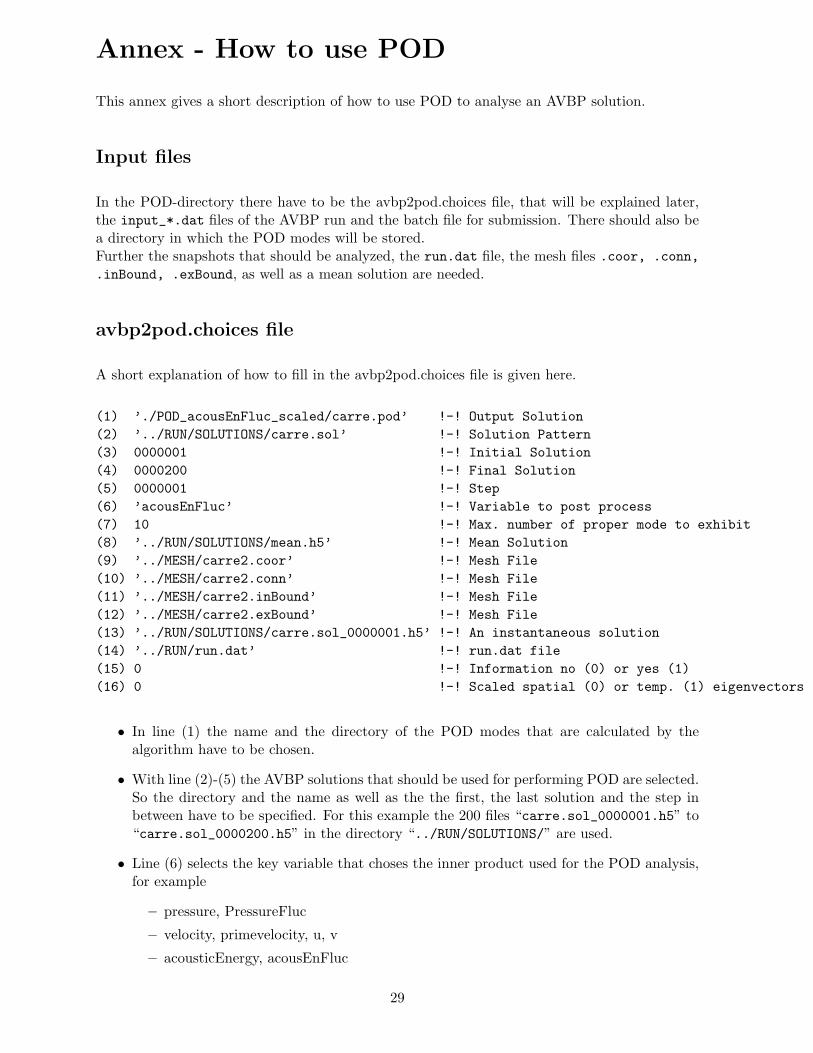
This annex gives a short description of how to use POD to analyse an AVBP solution.

Input files

In the POD-directory there have to be the avbp2pod.choices file, that will be explained later,the input_*.dat files of the AVBP run and the batch file for submission. There should also bea directory in which the POD modes will be stored.Further the snapshots that should be analyzed, the run.dat file, the mesh files .coor, .conn,.inBound, .exBound, as well as a mean solution are needed.

avbp2pod.choices file

A short explanation of how to fill in the avbp2pod.choices file is given here.

(1) ’./POD_acousEnFluc_scaled/carre.pod’ !-! Output Solution(2) ’../RUN/SOLUTIONS/carre.sol’ !-! Solution Pattern(3) 0000001 !-! Initial Solution(4) 0000200 !-! Final Solution(5) 0000001 !-! Step(6) ’acousEnFluc’ !-! Variable to post process(7) 10 !-! Max. number of proper mode to exhibit(8) ’../RUN/SOLUTIONS/mean.h5’ !-! Mean Solution(9) ’../MESH/carre2.coor’ !-! Mesh File(10) ’../MESH/carre2.conn’ !-! Mesh File(11) ’../MESH/carre2.inBound’ !-! Mesh File(12) ’../MESH/carre2.exBound’ !-! Mesh File(13) ’../RUN/SOLUTIONS/carre.sol_0000001.h5’ !-! An instantaneous solution(14) ’../RUN/run.dat’ !-! run.dat file(15) 0 !-! Information no (0) or yes (1)(16) 0 !-! Scaled spatial (0) or temp. (1) eigenvectors

• In line (1) the name and the directory of the POD modes that are calculated by thealgorithm have to be chosen.

• With line (2)-(5) the AVBP solutions that should be used for performing POD are selected.So the directory and the name as well as the the first, the last solution and the step inbetween have to be specified. For this example the 200 files “carre.sol_0000001.h5” to“carre.sol_0000200.h5” in the directory “../RUN/SOLUTIONS/” are used.

• Line (6) selects the key variable that choses the inner product used for the POD analysis,for example

– pressure, PressureFluc

– velocity, primevelocity, u, v

– acousticEnergy, acousEnFluc

29

For more information about the different inner product see section 2, Eq. (8)-(10).

• In line (7) the maximum number of POD modes that should be calculated is chosen. Thiscan be a difficult a priori choice as the corresponding eigenvalues are useful hint of theimportance of a mode. But they are not known before running the POD algorithm.

• The lines (8)-(14) have to be filled in with the information of the AVBP run.

• With line (15) additional information about the the temporal eigenvectors and -valuescan be obtained. The correlation matrix is a real symmetric matrix and should have realeigenvalues. Due to the numerical solving of the eigenvalue problem complex eigenvectorsand -values can occur. For example if the key variable “pressure” is used, the mean valueis very big compared to the fluctuation. So the entries of the correlation matrix are quitesimilar compared to their absolut size, which can cause difficulties in solving the eigenvalueproblem. Not all eigenvalues and -vectors are used in the POD algorithm (see line (7)),so there is only a warning if the ones used have an imaginay part. This imaginay part isskipped and the real part is put in the computation. If there is a (1) in this line informationabout these problems of all eigenvectors and -values is displayed, not only for those thatare actually used.

• Line (16) is for chosing the scaling. The method described in this report is for controlledscaling of the spatial eigenvectors (that is usually found in the theory for POD). To applythis method use “0” in this line. This leads to temporal eigenvectors, that differ signifi-cantly in scale. It can be used to compare the importance of the POD modes. For this caseit is necessary to divide by the eigenvalues in the POD algorithm, that can be very small.If they are smaller than 10−15 this division is not performed any more with a warning. Toavoid this less POD modes can be calculated. These modes without proper scaling shouldnot be used.Another way to avoid this problem is not to control the scaling of the spatial but thetemporal eigenvector (use “1” in this line). This leads to similar temporal eigenvectors insize and the information of the importance is contained in the POD modes, that will differin scale. An advantage is that the division by the eigenvalue is not necessary in this case.

Output files

The output files of POD are

• pod_matrix.dat (the correlation matrix),

• pod_val_p.dat (the eigenvalues),

• pod_vect_p.dat (the temporal eigenvectors),

• POD modes in the selected directory with the selected name(for example ./POD_acousEnFluc_scaled/carre.pod_0000001.h5),

• it is recommended to redirect the standard output to a file where warnings and informationare displayed.

The POD modes are given in an AVBP mean format so they can be visualized using a visualscript.

30

List of Figures

1 Grid used for AVBP solution, “perfect” square . . . . . . . . . . . . . . . . . . . 6

2 Eigenvalues, “perfect” square, pressure fluctuation . . . . . . . . . . . . . . . . . 7

3 First temporal eigenvector evolution, “perfect” square, pressure fluctuation . . . 7

4 First POD mode, “perfect” square, pressure fluctuation . . . . . . . . . . . . . . 8

5 Eigenvalues, “perfect” square, velocity fluctuation . . . . . . . . . . . . . . . . . . 8

6 First temporal eigenvector evolution, “perfect” square, pressure and velocity fluc-tuation . . . . . . . . . . . . . . . . . . . . . . . . . . . . . . . . . . . . . . . . . . 9

7 First POD mode, “perfect” square, velocity fluctuation . . . . . . . . . . . . . . . 9

8 Eigenvalues, “perfect” square, acoustic energy fluctuation . . . . . . . . . . . . . 10

9 First and second temporal eigenvector, “perfect” square, acoustic energy fluctuation 11

10 First and second temporal eigenvector evolution, “perfect” square, acoustic energyfluctuation . . . . . . . . . . . . . . . . . . . . . . . . . . . . . . . . . . . . . . . . 11

11 First POD mode, “perfect” square, acoustic energy fluctuation . . . . . . . . . . 12

12 Second POD mode, “perfect” square, acoustic energy fluctuation . . . . . . . . . 12

13 Eigenvalues, square . . . . . . . . . . . . . . . . . . . . . . . . . . . . . . . . . . . 15

14 First and second temporal eigenvector, square . . . . . . . . . . . . . . . . . . . . 16

15 Third and fourth temporal eigenvector, square . . . . . . . . . . . . . . . . . . . 16

16 First and second temporal eigenvector evolution, square . . . . . . . . . . . . . . 16

17 Third and fourth temporal eigenvector evolution, square . . . . . . . . . . . . . . 17

18 First and third temporal eigenvector evolution, normalized, square . . . . . . . . 17

19 First POD mode, square . . . . . . . . . . . . . . . . . . . . . . . . . . . . . . . . 17

20 Second POD mode, square . . . . . . . . . . . . . . . . . . . . . . . . . . . . . . . 18

21 Third POD mode, square . . . . . . . . . . . . . . . . . . . . . . . . . . . . . . . 18

22 Fourth POD mode, square . . . . . . . . . . . . . . . . . . . . . . . . . . . . . . . 19

23 Eigenvalues, square, 3 initial modes . . . . . . . . . . . . . . . . . . . . . . . . . . 21

24 First, second and third temporal eigenvector evolution, square, 3 initial modes . 22

25 First and second POD mode, square, 3 initial modes . . . . . . . . . . . . . . . . 22

26 Third POD mode, square, 3 initial modes . . . . . . . . . . . . . . . . . . . . . . 22

27 Grid used for AVBP solution, L-Shape . . . . . . . . . . . . . . . . . . . . . . . . 23

28 Eigenvalues, L-Shape . . . . . . . . . . . . . . . . . . . . . . . . . . . . . . . . . . 25

29 First and second temporal eigenvector evolution, L-Shape . . . . . . . . . . . . . 25

31

30 Third and fourth temporal eigenvector evolution, L-Shape . . . . . . . . . . . . . 26

31 First and third temporal eigenvector evolution, normalized, L-Shape . . . . . . . 26

32 First POD mode, L-Shape . . . . . . . . . . . . . . . . . . . . . . . . . . . . . . . 27

33 Second POD mode, L-Shape . . . . . . . . . . . . . . . . . . . . . . . . . . . . . . 27

34 Third POD mode, L-Shape . . . . . . . . . . . . . . . . . . . . . . . . . . . . . . 28

35 Fourth POD mode, L-Shape . . . . . . . . . . . . . . . . . . . . . . . . . . . . . . 28

References

[1] Berkooz, G., Holmes, P., and Lumley, J. The Proper Orthogonal Decomposition inthe Analysis of Turbulent Flows. Annual Review of Fluid Mechanics 25 (1993), 539–575.

[2] Braud, C. Etude de la dynamique d’un ecoulement a cisaillements croises: interactioncouche de melange–sillage. PhD thesis, Poitiers University, France, 2003.

[3] Chatterjee, A. An introduction to the proper orthogonal decomposition. Current Science78, 7 (2000), 808–817.

[4] Cordier, L., and Bergmann, M. Proper Orthogonal Decomposition: an Overview. PostProcessing of Experimental and Numerical Data (2003), 1–45. Lecture Series 2003/2004,von Karman Institut for Fluid Dynamics.

[5] Holmes, P., Lumley, J., and Berkooz, G. Turbulence, Coherent Structures, Dynami-cal Systems and Symmetry. Cambridge Monnographs on Mechanics. Cambridge UniversityPress (1996).

[6] Huang, Y., Wang, S., and Yang, V. Systematic Analysis of Lean-Premixed Swirl-Stabilized Combustion. AIAA Journal 44, 4 (2006), 724–740.

[7] Lumley, J. The structure of inhomogeneous turbulent flows. Atmospheric Turbulence andRadio Wave Propagation (1967), 166–178. ed. A. Yaglom and V. Tatarski.

[8] Poinsot, T., and Veynante, D. Theoretical and Numerical Combustion. Edwards,2001.

[9] Roux, A., Gicquel, L., Sommerer, Y., and Poinsot, T. Large eddy simulation ofmean and oscillating flow in side-dump ramjet combustor. Combust. Flame in press (2007).

[10] Roux, S. Application de la decomposition en modes propres a des calculs de simulations auxgrandes echelles. Rapport de stage 2eme annee Ingenieur - ENSEEIHT WN/CFD/06/61,CERFACS, September 28 2006.

[11] Rowley, C., Colonius, T., and Murray, R. Model Reduction for Compressible FlowsUsing POD and Galerkin Projection. Physica. D 189 (2004), 115–129.

[12] Silva, C. AVSP Quality Program Form, Square cavity. Tech. rep., CERFACS, InternalDocument, 2007. AVSP V4.0.

[13] Sirovich, L. Turbulence and the Dynamics of Coherent Structures. Part 1: CoherentStructures. Quarterly of Applied Mathematics 45, 3 (1987), 561–571.

32

[14] Wieczorek, K. AVSP Quality Program Form, L-Shape. Tech. rep., CERFACS, InternalDocument, 2007. AVSP V4.0.

33

Applications of the Proper Orthogonal Decomposition Methodcfdbib/repository/WN_CFD_07_97.pdf ·...

Documents

Transcript of Applications of the Proper Orthogonal Decomposition Methodcfdbib/repository/WN_CFD_07_97.pdf ·...