
APPLICATIONS OF MODEL PREDICTIVE CONTROL TO VEHICLE ...rv794bn8004/beal_elec... · applications of...
161
APPLICATIONS OF MODEL PREDICTIVE CONTROL TO VEHICLE DYNAMICS FOR ACTIVE SAFETY AND STABILITY A DISSERTATION SUBMITTED TO THE DEPARTMENT OF MECHANICAL ENGINEERING AND THE COMMITTEE ON GRADUATE STUDIES OF STANFORD UNIVERSITY IN PARTIAL FULFILLMENT OF THE REQUIREMENTS FOR THE DEGREE OF DOCTOR OF PHILOSOPHY Craig E. Beal August 2011
Transcript of APPLICATIONS OF MODEL PREDICTIVE CONTROL TO VEHICLE ...rv794bn8004/beal_elec... · applications of...

APPLICATIONS OF MODEL PREDICTIVE CONTROL TO
VEHICLE DYNAMICS FOR ACTIVE SAFETY AND STABILITY
A DISSERTATION
SUBMITTED TO THE DEPARTMENT OF MECHANICAL
ENGINEERING
AND THE COMMITTEE ON GRADUATE STUDIES
OF STANFORD UNIVERSITY
IN PARTIAL FULFILLMENT OF THE REQUIREMENTS
FOR THE DEGREE OF
DOCTOR OF PHILOSOPHY
Craig E. Beal
August 2011

http://creativecommons.org/licenses/by-nc-sa/3.0/us/
This dissertation is online at: http://purl.stanford.edu/rv794bn8004
© 2011 by Craig Earl Beal. All Rights Reserved.
Re-distributed by Stanford University under license with the author.
This work is licensed under a Creative Commons Attribution-Noncommercial-Share Alike 3.0 United States License.
ii

I certify that I have read this dissertation and that, in my opinion, it is fully adequatein scope and quality as a dissertation for the degree of Doctor of Philosophy.
J Gerdes, Primary Adviser
I certify that I have read this dissertation and that, in my opinion, it is fully adequatein scope and quality as a dissertation for the degree of Doctor of Philosophy.
Stephen Boyd, Co-Adviser
I certify that I have read this dissertation and that, in my opinion, it is fully adequatein scope and quality as a dissertation for the degree of Doctor of Philosophy.
Sven Beiker
Approved for the Stanford University Committee on Graduate Studies.
Patricia J. Gumport, Vice Provost Graduate Education
This signature page was generated electronically upon submission of this dissertation in electronic format. An original signed hard copy of the signature page is on file inUniversity Archives.
iii

This dissertation is dedicated to my family.
iv

Abstract
Each year in the United States, thousands of lives are lost as a result of loss of control
crashes [48]. Production driver assistance systems such as electronic stability control
(ESC) have been shown to be highly effective in preventing many of these automotive
crashes, yet these systems rely on a sensor suite that yields limited information about
the road conditions and vehicle motion. Furthermore, ESC systems rely on gains and
thresholds that are tuned to yield good performance without feeling overly restrictive
to the driver. This dissertation presents an alternative approach to providing sta-
bilization assistance to the driver which leverages additional information about the
vehicle and road that may be obtained with advanced estimation techniques.
This new approach is based on well-known and robust vehicle models and utilizes
phase plane analysis techniques to describe the limits of stable vehicle handling,
alleviating the need for hand tuning of gains and thresholds. The resulting state space
within the computed handling boundaries is referred to as a safe handling envelope.
In addition to the boundaries being straightforward to calculate, this approach has
the benefit of offering a way for the designer of the system to directly adjust the
controller to accomodate the preferences of different drivers.
A model predictive control structure capable of keeping the vehicle within the
safe handling boundaries is the final component of the envelope control system. This
dissertation presents the design of a controller that is capable of smoothly and progres-
sively augmenting the driver steering input to enforce the boundaries of the envelope.
The model predictive control formulation provides a method for making trade-offs be-
tween enforcing the boundaries of the envelope, minimizing disruptive interventions,
and tracking the driver’s intended trajectory.
v

Experiments with a steer-by-wire test vehicle demonstrate that the model pre-
dictive envelope control system is capable of operating in conjunction with a human
driver to prevent loss of control of the vehicle while yielding a predictable vehicle
trajectory. These experiments considered both the ideal case of state information
from a GPS/INS system and an a priori friction estimate as well as a real-world im-
plementation estimating the vehicle states and friction coefficient from steering effort
and inertial sensors. Results from the experiments demonstrated a controller that is
tolerant of vehicle and tire parameterization errors and works well over a wide range
of conditions. When real time sensing of the states and friction properties is enabled,
the results show that coupling of the controller and estimator is possible and the
model predictive control structure provides a mechanism for minimizing undesirable
coupled dynamics through tuning of intuitive controller parameters.
The model predictive control structure presented in this dissertation may also be
considered as a general framework for vehicle control in conjunction with a human
driver. The structure utilized for envelope control may also be used to restrict other
vehicle states for safety and stability. Results are presented in this dissertation to
show that a model predictive controller can coordinate a secondary actuator to alter
the planar states and reduce the energy transferred into the roll modes of the vehicle.
The systematic approach to vehicle stabilization presented in this dissertation has
the potential to improve the design methodology for future systems and form the
basis for the inclusion of more advanced functions as sensing and computing capa-
bilities improve. The envelope control system presented here offers the opportunity
to advance the state of the art in stabilization assistance and provides a way to help
drivers of all skill levels maintain control of their vehicle.
vi

Acknowledgement
Writing a dissertation is a time of great reflection, not only upon the work presented
in the dissertation, but about the entire graduate student experience. During the
time that I have spent earning my Ph.D., I’ve come to realize that earning the degree
is only possible with an immense amount of support coming from people in all aspects
of life. Therefore, I wish to generally thank everyone for their roles in helping me
obtain my doctoral degree.
The list of people to whom I owe my gratitute would probably exceed the length
of this dissertation if I described the contributions of each individual, but I would
like to acknowledge a few groups and people who played particularly large parts in
what I have accomplished. First I must recognize my Stanford friends. In a first year
full of sleep deprived nights while completing 24 hour exams and quarter-long class
projects, these were the people who stuck together, encouraged me, and helped me
blow off steam when each milestone was met. Those who continued on for their Ph.D.
or graduated and stayed in the area are much of the reason that Stanford will always
feel like home to me.
I would also like to express my appreciation to my reading and defense committees.
After many tense days of preparation leading up to my defense, the presentation and
question session were highly enjoyable. Many thanks are deserved by Professors Steve
Rock and Tom Kenny for joining my committee and contributing valuable insight
during the closed session. I am also grateful to Professor Stephen Boyd for agreeing
to serve on my reading committee and providing much insight about model predictive
control throughout the development of my dissertation work. Likewise, I must thank
Sven Beiker for sitting on my reading committee and providing excellent feedback
vii

on my work. His test driving experience was instrumental in the formulation of a
controller that offers a skilled driver the opportunity to push the vehicle to the limits
of handling.
Aside from my defense and reading committees, there are a number of people who
provided assistance and feedback to me throughout my graduate career. In particular,
my labmates at the DDL were always willing to listen to my thoughts, critique my
ideas, and offer suggestions to help push me forward when I was stuck. They were
also there to socialize, swap airport rides, and celebrate successes with beers at the
Treehouse. Josh Switkes, Chris Carlson, Chris Gadda, Shad Laws, and Matt Roelle
were instrumental in preparing me for the qualifying exam and life as a Dynamic
Design Lab member. My cohorts in the lab, Adam Jungkunz, Carrie Bobier, Hsien-
Hsin Liao, and Rami Hindiyeh have made the time that I spent in the lab pass far
too quickly. I will greatly miss the daily interactions of working in MERL. Finally, I
would like to express great appreciation to Jacob Mattingly, who provided me with
both his real time convex optimization code and a great deal of support as I attempted
to figure out how to use it.
Among the greatest challenges in obtaining a doctoral degree is the process of
developing a research topic. I can’t thank Chris Gerdes enough for his help in this
and all other aspects of my graduate student experience. Chris was not just an
advisor, but a mentor and a friend. Never once during my tenure in the Dynamic
Design Lab did I have to worry about having the resources to explore an interesting
idea and ultimately I have to say that obtaining a Ph.D. at Stanford was by far “the
coolest thing I could do.”
Yet pursuing the coolest things would never have been possible without the sup-
port of my family. My parents and grandparents stressed the value of education
throughout my childhood and supported me in all my endeavors. When I graduated
from high school, they provided me with the financial support that allowed me to pur-
sue my undergraduate degree at Bucknell. It was at Bucknell that I met professors
Steve Shooter and Keith Buffinton, who started me down the path toward graduate
school and a career in academia. These connections would never have been made
were it not for the love, support, and assistance of my parents and grandparents.
viii

Finally, I must thank Kelly Beal, my wonderfully supportive wife. It took an
incredible amount of faith in me for her to leave her home and family to come with
me to Stanford. In the six years we lived at Stanford, she earned a masters degree,
became a highly respected member of the social studies faculty at Mills High School,
and brought Ella, our beautiful daughter, into our lives. Without her, my Stanford
career would have been a drastically different experience. I doubt that I can ever
express my gratitude for being both my champion and my critic, the deep pockets
behind our countless adventures, and my best friend on this incredible journey.
ix

Contents
Dedication iv
Abstract v
Acknowledgement vii
1 Introduction 1
1.1 Motivation . . . . . . . . . . . . . . . . . . . . . . . . . . . . . . . . . 1
1.2 Background . . . . . . . . . . . . . . . . . . . . . . . . . . . . . . . . 3
1.2.1 Overview of the Vehicle Stability Problem . . . . . . . . . . . 3
1.2.2 Development of Electronic Stability Control . . . . . . . . . . 6
1.2.3 Friction and State Estimation Techniques . . . . . . . . . . . 9
1.2.4 Envelope Protection in Aircraft . . . . . . . . . . . . . . . . . 10
1.2.5 Vehicle Control with Model Predictive Control . . . . . . . . . 11
1.2.6 Analysis of Unstable Vehicle Dynamics . . . . . . . . . . . . . 12
1.3 Dissertation Contributions . . . . . . . . . . . . . . . . . . . . . . . . 14
1.3.1 Instability Analysis and Criteria for Safe Handling . . . . . . . 15
1.3.2 Envelope Control for Enforcing Envelope Boundaries . . . . . 15
1.3.3 Guarantees of Vehicle Behavior under Envelope Control . . . . 16
1.3.4 Integration of Real-Time Friction Estimation . . . . . . . . . . 16
1.3.5 Extension of Envelope Control to Roll Dynamics . . . . . . . . 17
1.4 Dissertation Outline . . . . . . . . . . . . . . . . . . . . . . . . . . . 17
x

2 Vehicles and Models 20
2.1 Pneumatic Tires . . . . . . . . . . . . . . . . . . . . . . . . . . . . . 20
2.1.1 Brush Tire Model . . . . . . . . . . . . . . . . . . . . . . . . . 21
2.1.2 Linear Tire Model . . . . . . . . . . . . . . . . . . . . . . . . 26
2.2 Chassis Models . . . . . . . . . . . . . . . . . . . . . . . . . . . . . . 27
2.2.1 Four Wheel Yaw-Roll Model . . . . . . . . . . . . . . . . . . . 27
2.2.2 Bicycle Model . . . . . . . . . . . . . . . . . . . . . . . . . . . 28
2.2.3 Affine Force-Input Model . . . . . . . . . . . . . . . . . . . . . 31
2.2.4 Linearized Roll Model . . . . . . . . . . . . . . . . . . . . . . 33
2.2.5 Summary of Models . . . . . . . . . . . . . . . . . . . . . . . 34
2.3 P1 By-Wire Test Vehicle . . . . . . . . . . . . . . . . . . . . . . . . . 35
2.4 Experimental Testing . . . . . . . . . . . . . . . . . . . . . . . . . . . 37
3 Vehicle Instability 38
3.1 Instability Dynamics . . . . . . . . . . . . . . . . . . . . . . . . . . . 38
3.2 Defining Boundaries of Unstable Regions . . . . . . . . . . . . . . . . 46
3.2.1 Defining a Safe Handling Envelope . . . . . . . . . . . . . . . 47
3.2.2 Alternative Envelopes . . . . . . . . . . . . . . . . . . . . . . 49
3.3 Discussion . . . . . . . . . . . . . . . . . . . . . . . . . . . . . . . . . 54
4 Envelope Control 55
4.1 Control Strategy . . . . . . . . . . . . . . . . . . . . . . . . . . . . . 55
4.1.1 MPC with the Affine Force-Input Model . . . . . . . . . . . . 56
4.1.2 Envelope Boundaries . . . . . . . . . . . . . . . . . . . . . . . 58
4.1.3 Tracking Driver Intent . . . . . . . . . . . . . . . . . . . . . . 59
4.1.4 Controller Implementation . . . . . . . . . . . . . . . . . . . . 60
4.1.5 Real Time MPC Implementation . . . . . . . . . . . . . . . . 62
4.2 Results and Discussion . . . . . . . . . . . . . . . . . . . . . . . . . . 63
4.2.1 Experiment: Limit Slalom Maneuver . . . . . . . . . . . . . . 63
4.2.2 Simulation: Slalom with Friction Variation . . . . . . . . . . . 65
4.2.3 Experiment: Limit Cornering with Rear Drive Torques . . . . 67
4.2.4 Experiment: Control Performance with Linear Model . . . . . 70
xi

4.2.5 Experiment: Control with Wide Slip Boundaries . . . . . . . . 72
4.3 Guaranteeing Controller Action . . . . . . . . . . . . . . . . . . . . . 74
4.3.1 Envelope Invariance Proof . . . . . . . . . . . . . . . . . . . . 74
4.3.2 Envelope Attraction . . . . . . . . . . . . . . . . . . . . . . . 80
4.3.3 Feasible Trajectories . . . . . . . . . . . . . . . . . . . . . . . 81
4.3.4 Effect of Actuator Limits . . . . . . . . . . . . . . . . . . . . . 84
4.4 Summary . . . . . . . . . . . . . . . . . . . . . . . . . . . . . . . . . 85
5 Real Time Estimation 87
5.1 Estimation Technique . . . . . . . . . . . . . . . . . . . . . . . . . . . 87
5.1.1 Slip Angle Estimation . . . . . . . . . . . . . . . . . . . . . . 88
5.1.2 Peak Force Estimation . . . . . . . . . . . . . . . . . . . . . . 89
5.1.3 Practical Considerations . . . . . . . . . . . . . . . . . . . . . 92
5.2 Estimator Results . . . . . . . . . . . . . . . . . . . . . . . . . . . . . 94
5.2.1 Estimator Input Data Characteristics . . . . . . . . . . . . . . 94
5.2.2 Slip Angle Observer Results . . . . . . . . . . . . . . . . . . . 97
5.2.3 Pneumatic Trail and Friction Results . . . . . . . . . . . . . . 98
5.3 Coupled Controller/Estimator Design . . . . . . . . . . . . . . . . . . 100
5.4 Control Results with Real Time Estimation . . . . . . . . . . . . . . 101
5.4.1 System Convergence . . . . . . . . . . . . . . . . . . . . . . . 102
5.4.2 Coupled Operation . . . . . . . . . . . . . . . . . . . . . . . . 102
5.4.3 Controller Parameter Sensitivity . . . . . . . . . . . . . . . . . 105
5.4.4 “Locked-low” Operating Regime . . . . . . . . . . . . . . . . . 107
5.5 Discussion . . . . . . . . . . . . . . . . . . . . . . . . . . . . . . . . . 109
6 Extensions of Envelope Control 110
6.1 Control of Roll Dynamics . . . . . . . . . . . . . . . . . . . . . . . . 110
6.1.1 Control Approach . . . . . . . . . . . . . . . . . . . . . . . . . 111
6.1.2 MPC Expression . . . . . . . . . . . . . . . . . . . . . . . . . 113
6.1.3 Real Time MPC Implementation . . . . . . . . . . . . . . . . 115
6.2 Simulation Results . . . . . . . . . . . . . . . . . . . . . . . . . . . . 116
6.2.1 Roll Control Objective . . . . . . . . . . . . . . . . . . . . . . 116
xii

6.2.2 Baseline Dynamics . . . . . . . . . . . . . . . . . . . . . . . . 116
6.2.3 Independent Wheel Torque Control . . . . . . . . . . . . . . . 119
6.2.4 Rear Wheel Steering Control . . . . . . . . . . . . . . . . . . . 120
6.3 Discussion . . . . . . . . . . . . . . . . . . . . . . . . . . . . . . . . . 123
7 Conclusions 125
7.1 Summary . . . . . . . . . . . . . . . . . . . . . . . . . . . . . . . . . 125
7.1.1 Safe Handling Envelopes . . . . . . . . . . . . . . . . . . . . . 125
7.1.2 Real Time Model Predictive Control . . . . . . . . . . . . . . 126
7.1.3 Real Time Friction and Sideslip Estimation . . . . . . . . . . 126
7.1.4 Extension of the Envelope Control Technique . . . . . . . . . 126
7.2 Future Work . . . . . . . . . . . . . . . . . . . . . . . . . . . . . . . . 127
7.2.1 Driver Feedback . . . . . . . . . . . . . . . . . . . . . . . . . . 127
7.2.2 Controller Complexity . . . . . . . . . . . . . . . . . . . . . . 127
7.2.3 Handling Environmental Constraints . . . . . . . . . . . . . . 128
7.3 Outlook . . . . . . . . . . . . . . . . . . . . . . . . . . . . . . . . . . 128
A X1 Experimental Test Vehicle 130
A.1 Physical Design . . . . . . . . . . . . . . . . . . . . . . . . . . . . . . 130
A.1.1 Modularity Concept . . . . . . . . . . . . . . . . . . . . . . . 131
A.1.2 Actuation Opportunities . . . . . . . . . . . . . . . . . . . . . 133
A.1.3 Drivetrain . . . . . . . . . . . . . . . . . . . . . . . . . . . . . 133
A.2 Electrical Design . . . . . . . . . . . . . . . . . . . . . . . . . . . . . 134
A.2.1 Power System . . . . . . . . . . . . . . . . . . . . . . . . . . . 134
A.2.2 Data Network . . . . . . . . . . . . . . . . . . . . . . . . . . . 134
A.3 Discussion . . . . . . . . . . . . . . . . . . . . . . . . . . . . . . . . . 135
Bibliography 136
xiii

List of Tables
2.1 Vehicle Models . . . . . . . . . . . . . . . . . . . . . . . . . . . . . . 35
2.2 Parameters for the P1 test vehicle . . . . . . . . . . . . . . . . . . . . 36
4.1 Description of Envelope Controller Parameters . . . . . . . . . . . . . 61
4.2 Envelope Controller Parameters with AFI Model . . . . . . . . . . . . 65
4.3 Envelope Controller Parameters with Linear Model . . . . . . . . . . 69
6.1 Description of Roll Controller Parameters . . . . . . . . . . . . . . . . 115
6.2 Independent Wheel Torque Roll Controller Parameters . . . . . . . . 119
6.3 Rear Steering Roll Controller Parameters . . . . . . . . . . . . . . . . 121
xiv

List of Figures
1.1 Vehicle Dynamics Axes and Coordinates . . . . . . . . . . . . . . . . 4
1.2 Electronic Stability Control Action . . . . . . . . . . . . . . . . . . . 7
1.3 Phase Portrait Showing Instability Dynamics . . . . . . . . . . . . . . 13
2.1 Tire Curve - Two Coefficient Brush Model . . . . . . . . . . . . . . . 22
2.2 Force Distribution in the Contact Path . . . . . . . . . . . . . . . . . 23
2.3 Combined Tire Force Limits . . . . . . . . . . . . . . . . . . . . . . . 25
2.4 Comparison of Linear and Brush Tire Models . . . . . . . . . . . . . 26
2.5 Four-wheel Yaw-Roll Model . . . . . . . . . . . . . . . . . . . . . . . 28
2.6 The Bicycle Model . . . . . . . . . . . . . . . . . . . . . . . . . . . . 29
2.7 P1 Steer and Drive By-Wire Research Testbed . . . . . . . . . . . . . 36
3.1 Phase Portraits of a Neutral Steering Vehicle . . . . . . . . . . . . . . 40
3.2 Phase Portraits of an Understeering Vehicle . . . . . . . . . . . . . . 42
3.3 Phase Portraits of an Oversteering Vehicle . . . . . . . . . . . . . . . 43
3.4 Vehicle Spin-out Data in the Phase Plane . . . . . . . . . . . . . . . . 44
3.5 Phase Portrait of a Neutral Steering Vehicle at Higher Speed . . . . . 45
3.6 Phase Portrait with Model Predictive Envelope Controller . . . . . . 48
3.7 Vehicle Derivatives on Envelope Boundaries . . . . . . . . . . . . . . 49
3.8 Handling Envelope with Wider Slip Bounds . . . . . . . . . . . . . . 51
3.9 Handling Envelope with Extra Allowable Yaw Rate . . . . . . . . . . 52
3.10 Yaw Sideslip Handling Envelope . . . . . . . . . . . . . . . . . . . . . 53
4.1 MPC Block Diagram . . . . . . . . . . . . . . . . . . . . . . . . . . . 57
xv

4.2 MPC Envelope Controller Boundaries . . . . . . . . . . . . . . . . . . 58
4.3 Experimental Results from Slalom Maneuver . . . . . . . . . . . . . . 64
4.4 Simulated Results from Slalom Maneuver . . . . . . . . . . . . . . . . 66
4.5 Experimental Results from Cornering with Torque Disturbances . . . 68
4.6 Experimental Results from Lift-off Oversteer Maneuver . . . . . . . . 71
4.7 Experimental Results with Wide Rear Slip Angle Boundaries . . . . . 73
4.8 Four quadrants of the state space used for the proof . . . . . . . . . . 78
4.9 Feasible Envelope Re-entry Trajectory . . . . . . . . . . . . . . . . . 83
4.10 Slew Distance for Change of Tire Force . . . . . . . . . . . . . . . . . 84
4.11 Envelope Re-entry with Slew Rate Limitation . . . . . . . . . . . . . 85
5.1 Steering Axis Geometry . . . . . . . . . . . . . . . . . . . . . . . . . 90
5.2 Lateral Force and Linear Pneumatic Trail Models . . . . . . . . . . . 92
5.3 Coupled Sideslip and Friction Estimator Flowchart . . . . . . . . . . 93
5.4 Representative Inertial Measurements . . . . . . . . . . . . . . . . . . 95
5.5 Representative Steering Derivative . . . . . . . . . . . . . . . . . . . . 95
5.6 Representative Aligning Moments . . . . . . . . . . . . . . . . . . . . 95
5.7 Aligning Moment Frequency Content . . . . . . . . . . . . . . . . . . 96
5.8 Slip Angle Estimates . . . . . . . . . . . . . . . . . . . . . . . . . . . 97
5.9 Calculated Pneumatic Trail . . . . . . . . . . . . . . . . . . . . . . . 99
5.10 Calculated Friction Coefficient . . . . . . . . . . . . . . . . . . . . . . 100
5.11 Calculated Friction Coefficient . . . . . . . . . . . . . . . . . . . . . . 101
5.12 Friction Convergence under Control . . . . . . . . . . . . . . . . . . . 103
5.13 Control with Real Time Estimation . . . . . . . . . . . . . . . . . . . 104
5.14 Over-response with Real Time Estimation . . . . . . . . . . . . . . . 106
5.15 “Locked-low” Coupled System Operation . . . . . . . . . . . . . . . . 108
6.1 Vehicle State and Input Trajectories for Baseline (Inactive) Case . . . 117
6.2 Vehicle State Trajectories for Drive/Brake Torque Controller . . . . . 118
6.3 Inputs for Controlled Fast Ramp Steer with Differential Drive . . . . 118
6.4 Vehicle State Trajectories for Rear Wheel Steering Controller . . . . . 122
6.5 Inputs for Controlled Fast Ramp Steer with Rear Wheel Steering . . 123
xvi

A.1 X1 Steer and Drive By-Wire Research Testbed . . . . . . . . . . . . . 131
A.2 Front-Middle-Rear Modularity Concept . . . . . . . . . . . . . . . . . 132
A.3 CAD Mockup of Modular Structure . . . . . . . . . . . . . . . . . . . 132
A.4 Electronic Modularity Concept . . . . . . . . . . . . . . . . . . . . . 135
xvii

Chapter 1
Introduction
1.1 Motivation
In the United States, the automobile is a foundation upon which many aspects of
daily life are built. Cars provide opportunities, including the freedom to live at a
distance from employers, the ability to travel, and even the option to express oneself
with choice of vehicle. The utility of the automobile is clear, and the proof lies in
approximately 2.9 trillion vehicle miles traveled in 2009 alone in the United States
[48]. However, the cost in human lives is also clear. In that same year, nearly 34
thousand people were killed and 2.2 million people were injured in the U.S. as a
result of vehicle crashes [48]. Often these crashes occur in unfavorable conditions
brought about due to the actions of the driver or interactions with the environment.
Excessive speed and sudden changes in surface friction due to gravel, snow, or ice are
commonly associated with these types of loss-of-control crashes. In these conditions,
the dynamics of the vehicle change drastically from those of normal everyday driving.
Unprepared drivers who must suddenly handle the vehicle in these challenging driving
regimes may fail to respond appropriately and lose control.
Automotive manufacturers have addressed this problem through the addition of
active safety systems in production vehicles. These systems, including Anti-Lock
Braking (ABS), Traction Control (TCS), Electronic Stability Control (ESC), and
Roll Stability Control (RSC) utilize control over the drive and brake systems of the
1

CHAPTER 1. INTRODUCTION 2
vehicle to augment the driver’s actions and improve the handling response of the
vehicle. Since their implementation, these systems have improved the ability of drivers
to maintain control of the vehicle and have resulted in significant reductions in the
human cost of automobiles. Studies of ESC by the National Highway Traffic Safety
Administration (NHTSA) have shown that ESC can be credited with a 36% reduction
in single-vehicle crashes among ESC-equipped vehicles in the United States [16].
Despite the effectiveness of these assistance systems, vehicle crashes resulting in
injuries and fatalities continue to occur. Therefore, future assistance systems must go
farther to help the driver of the vehicle. This may be enabled through the use of new
technologies that provide information about the environment, perhaps including road
conditions, obstacles, and other vehicles. One example is the adoption of Electric
Power Steering (EPS) in many production vehicles, which can be leveraged to obtain
information about the vehicle states and the road friction coefficient at a low cost
to the manufacturer. This information can be used in driver assistance systems to
increase the speed and accuracy of their response.
However, incorporating additional information is a challenge on its own. Current
production stability control systems utilize a limited suite of measurements, includ-
ing vehicle yaw rate, speed, lateral acceleration, and steering wheel position. These
measurements are reliable and readily available on production vehicles, but do not
yield a complete picture of the vehicle behavior. As a result, the actuation schema
currently used to alter the dynamics of the vehicle are relatively simple and rely on
high level logic and experimentally determined thresholds. Thousands of hours of
development have refined the implementations of these systems to tune the perfor-
mance and ensure the system works as desired. However, in order to incorporate more
information into these systems and provide more refined assistance to the driver, a
systematic approach to the analysis and development of controllers is needed. This
dissertation addresses the challenges of leveraging additional measurements to deter-
mine appropriate state boundaries for the vehicle and using model predictive control
to incorporate this additional information into the control of handling dynamics to
improve the safety of vehicles.

CHAPTER 1. INTRODUCTION 3
1.2 Background
1.2.1 Overview of the Vehicle Stability Problem
In order to define the task of the assistance system described in this dissertation, it is
necessary to define the basic dynamics that are relevant to maintaining control of the
vehicle. Figure 1.1 shows a vehicle with a coordinate system defined by ISO Standard
8855. The axes are fixed to the body of the vehicle with the positive x-axis pointing
in the forward direction, the positive y-axis to the driver’s left, and the positive z-
axis pointing upward. The vector V points in the direction of the vehicle’s velocity,
allowing for the definition of an angle, β, that is referred to as the sideslip angle. This
angle, the difference between the vehicle’s heading and its velocity, is a measure of
how sideways the vehicle is traveling. Clearly one often travels at highway speed with
zero sideslip angle, but it would be highly disconcerting to be traveling at the same
speed with a 90◦ sideslip angle. Therefore, restricting the sideslip angle to moderate
values is a critical task for stability control.
The other quantity of interest is the yaw rate, which is the rate at which the vehicle
rotates about the z-axis. If this yaw rate becomes too large and cannot be controlled,
the vehicle is said to have “spun out.” Therefore, this is the second quantity that
production ESC systems control to improve the stability of the vehicle. Like these
production systems, the driver assistance system presented in this dissertation also
uses the yaw rate and sideslip angles to improve the response of the vehicle at the
limits of its handling capabilities.
The yaw rate and sideslip angle of the vehicle are generated as a result of the
tire forces, which must be examined to understand the vehicle behavior when the
handling limitations are reached. These forces are generated by the adhesion of the
tire rubber to the road and can be used to drive the vehicle forward, brake it, or
generate lateral force to traverse a corner. Like the sideslip angle for the vehicle body,
a slip angle is defined between the heading of the wheel and its velocity. Because the
wheel is attached to the body of the vehicle, the lateral velocity and yaw rate of
the vehicle body result in tire slip angles. The lateral force generated by the tire
increases with the slip angle until the limits of the tire-road friction are reached. The

CHAPTER 1. INTRODUCTION 4
Z
XY
r Yaw Rate
Z
XY
!Sideslip V
Figure 1.1: Vehicle Dynamics Axes and Coordinates
driver controls the front force by increasing or decreasing the front slip angle with the
steering wheel, which results in sideslip and yaw rate motion of the vehicle. As these
motions occur, the rear axle also assumes a slip angle and produces forces. When the
vehicle is operating in a stable regime, these forces balance and the vehicle reaches
an equilibrium state.
Depending on the handling properties of the vehicle, including the mass distribu-
tion, the suspension set up, the tire characteristics, and other factors, these equilibria
will change as the steering angle changes, the vehicle speed increases, or the driver
utilizes some of the available friction force to accelerate or brake the vehicle. At some
point, the friction force is insufficient to maintain the equilibrium and the tires on
either axle begin to slide. Once the front tires reach this condition, the vehicle will
cease to turn any more and the vehicle is said to “understeer” the driver command at
the limits of handling. Conversely, if the rear tires lose grip first and the front tires
continue to generate high levels of force, the vehicle will turn too much and is said
to “oversteer” the driver command at the limits of handling. It is also possible for
both axles to lose grip simultaneously, which results in a large sideslip angle with a

CHAPTER 1. INTRODUCTION 5
low yaw rate and is referred to as “neutral” at the limits.
Fundamentally, the role of a stabilization system is to keep the vehicle from devi-
ating significantly from the behavior intended by the driver, such as in these oversteer
and understeer situations. However, this task is challenging since the true intent of
the driver may be infeasible given the handling limits of the vehicle, and in any case
cannot be measured. Therefore, the control system cannot simply track the driver’s
intent and the problem must be phrased in an alternate manner. For production sta-
bility control systems, this is addressed by inferring the desired vehicle behavior from
a linear model and a limited set of sensor measurements [70]. These measurements
are combined with estimates of the states and tire-road friction coefficient and are
compared to the linear model. Control action is taken if there is significant deviation.
This control scheme is highly effective, as seen from NHTSA analysis [48], and is
robust despite the limited sensor suite it utilizes. However, the reliance on deviation
from a linear model has two drawbacks. The first is that the stability control system
allows only dynamics that are close to the linear model, while skilled drivers may be
able to access other handling regimes. The second is that in order to avoid unnec-
essary interventions, the system must not take action until the vehicle behavior is
measureably outside of the stable regime.
While these types of trade-offs are required in a system for which it is feasible to
install on production vehicles, a number of technologies that have the capability of
providing additional information and actuation to stability control systems are ap-
pearing on the market. Among these enabling technologies are electric power steering
and steer-by-wire systems. With these actuators comes the ability to measure steer-
ing torque and with it, the ability to accurately estimate both the tire-road friction
coefficient and the vehicle sideslip angle [31].
With estimates of the states and friction characteristics available, it is possible
to take a different approach to vehicle stabilization. Most drivers are aware that
there exist inherent limitations in tire grip and therefore in the vehicle handling ca-
pabilities. Very highly skilled drivers can operate the vehicle at these limits without
allowing the vehicle to become unstable. However, less skilled drivers may exceed

CHAPTER 1. INTRODUCTION 6
these handling limits without realizing it, perhaps due to aggressive driving or emer-
gency maneuvering. With full-state feedback available, an advanced stabilization
system can accurately estimate these limitations and assist the driver in maintaining
the vehicle inside the bounds of the vehicle capabilities. Thus, the system may be re-
ferred to as an “envelope control” system, similar to the envelope protection systems
used in modern commercial aircraft [72]. This envelope control concept is the basis
for the assistance system described in this dissertation.
1.2.2 Development of Electronic Stability Control
The first assistance system to appear in production vehicles was Anti-Lock Braking
(ABS). This system utilizes a set of valves to modulate pressure to the brakes at
individual wheels. By rapidly applying and releasing brake pressure, the system
keeps the wheels rolling, simultaneously reducing stopping distance and improving
steerability of the vehicle. A fully-electronic, 4 channel system was first introduced
by Bosch and Mercedes-Benz in 1978 for trucks and the S-Class sedan [1]. Traction
Control (TCS), which prevents wheel-spin under engine torque, was developed later
using the same principles.
Once independent control of the wheels of the vehicle became possible, a new
control challenges was observed. On a surface with varied levels of grip between the
two sides of the vehicle, a naive ABS system attempting to provide maximum braking
on each wheel would produce different longitudinal forces on each side of the vehicle
and tend to apply a yaw moment that would cause an undesirable rotation of the
vehicle. While unintended in the split-µ braking situation, the resultant yaw motion
from differential longitudinal force on the left and right sides of the vehicle can be
leveraged to improve the response of the vehicle.
Production electronic stabilty control systems operate, like ABS, by actuating the
brakes of the vehicle independently to control the orientation of the vehicle. The
angle of the steering wheel, the vehicle speed, the rotation (yaw) rate of the vehicle,
and the lateral acceleration of the vehicle are readily measured with inexpensive
sensors. Based on a simple model of the vehicle dynamics, the driver’s intended

CHAPTER 1. INTRODUCTION 7
Figure 1.2: Electronic Stability Control Action [11]
vehicle behavior can be inferred from the vehicle speed and handwheel angle. The
ESC system compares these desired states to the measurements of yaw rate and
lateral acceleration to determine whether the driver requires assistance in stabilizing
the vehicle. If there is a significant difference between the inferred states and the
measurements, the system applies the brakes to correct the vehicle motion [70, 69].
There are two situations in which an ESC system intervenes to assist the driver.
The first is an understeer situation, where the vehicle fails to turn as much as the
driver would like. In this case, the ESC system may apply the inside rear brake
judiciously to make the vehicle rotate more. However, the system is typically pro-
grammed to do this only in severe understeering situations since the application of
the rear brake may cause the rear end of the car to lose grip and spin out. This is
the second situation that ESC systems help to prevent. When the vehicle begins to
oversteer, the ESC system can apply the outside front brake, which produces a yaw
moment that tends to straighten out the vehicle and prevents a spin.
Unfortunately, production ESC systems are limited by their reliance on a small set
of sensors that yield limited vehicle state information. As a result, they must react
only to deviations from a known model of the vehicle behavior and typically have
a “dead-band” where small deviations are allowed in order to prevent undesirable
interventions in non-critical situations. Additional information about the vehicle
CHAPTER 1. INTRODUCTION 8
states and the environment would be helpful in improving the system response, since
a system that could accurately gauge the situation would need not wait for a large
deviation from normal driving and could offer more subtle assistance to the driver.
In addition to the production ESC systems automotive manufacturers and sup-
pliers, many other authors have proposed methods for addressing the challenge of
controlling the planar dynamics of a vehicle in adverse situations. Manning and
Crolla give an excellent summary of the body of work in their 2007 survey paper [42].
Reviewing 68 salient papers, the authors divided the work into three general groups
by primary control objective. The groups included work that focused on control of
yaw rate, control of sideslip, and work that considered both states for control. When
looking at direct yaw control work, Manning and Crolla found that yaw stability sys-
tems are dominated by the use of model reference feedback control of the yaw rate
and note that attempting to track a linear reference model in the nonlinear handling
region can result in excessive actuator effort ([43, 41]). Chapter 3 of this dissertation
presents an analysis to show that while restricting the yaw rate is critical for stabil-
ity, tracking a reference model is unnecessary when appropriate yaw limits can be
calculated.
Among proposed techniques for control of the vehicle sideslip angle, Manning and
Crolla found that many researchers used differential braking due to its effectiveness
across a wide range of handling conditions. However, it was noted that some authors
argue that brake-based stability is overly invasive in the longitudinal dynamics of the
vehicle ([26, 63]). Finally, authors who considered both sideslip and yaw rate generally
treated the problem as a multi-objective control problem and either used multiple
actuators to address the separate objectives or used techniques such as sliding surface
control to trade off the objectives when only one actuator was used ([29, 66, 75]).
Interestingly, Manning and Crolla also noted that in the body of published work,
there are many theoretical studies that lack consideration of the practical aspects
involved in implementing the system and similarly many studies with excellent prac-
tical value but little detail in the analysis of the vehicle dynamics or the control laws.
This highlights the difficulty in developing a system that accurately accounts for the
CHAPTER 1. INTRODUCTION 9
nonlinear dynamics of the system and yet is straightforward enough for implementa-
tion on a vehicle. In controlling the sideslip dynamics of the vehicle with or without
coordination with yaw control, the authors also found that there was a significant
lack of work that incorporated real time estimation of the surface friction coefficient
and sideslip angle.
1.2.3 Friction and State Estimation Techniques
One of the reasons that production ESC systems use the model following control
approach that Manning and Crolla mention is that they lack information about the
full capabilities of the vehicle on the road surface. However, given full-state feedback
for the vehicle and the tire-road friction coefficient, it is possible to define limits to
form a stable vehicle handling envelope.
There have been a variety of investigators who have developed techniques for pro-
viding the required state and friction information. Full-state feedback of the vehicle
states can be provided with GPS hardware. Given the yaw angle, yaw rate, and
the direction of the vehicle travel, a full description of the planar vehicle dynamics
is possible [57, 8]. However, the equipment currently required to do this level of
state feedback is expensive and impractical for a production vehicle and is subject to
drop-out in areas where good visibility of the GPS satelite constellation is obsured.
Therefore, an estimation technique that relies on commonly installed vehicle sensors
is necessary to allow for advanced driver assistance on mass-produced vehicles. Sev-
eral authors have proposed sideslip angle estimation schemes, but the foundation for
these estimators are accurate tire models, which cannot be assumed in the presence
of varying road conditions, tire wear, variable vehicle loading, and other variable con-
ditions [37, 64, 71, 74]. Therefore, an estimate of the tire forces is simultaneously
needed to complete the description of the vehicle behavior in all conditions.
Work by Sakai points out the challenges in developing accurate estimates of the tire
forces. Because the tire characteristics change with a huge number of factors including
normal variations in tread wear, inflation pressure, temperature, and normal load, it
is impractical to use a parameterized tire model to estimate tire-road friction [58].

CHAPTER 1. INTRODUCTION 10
Therefore, alternative approaches such as those based on longitudinal tire slip have
been proposed, utilizing known excitation of the wheel dynamics to estimate friction
coefficients [23, 34, 54]. Other authors have utilized the lateral dynamics of the vehicle
for excitation, but require lateral accelerations near the limit of the vehicle capability
before obtaining accurate friction estimates, rendering them less useful for predicting
the limits of the vehicle handling before reaching them [2, 22]. For the purposes of
preventing the vehicle from developing unstable dynamics, a technique that provides
an estimate of the available friction at lower lateral accelerations is needed.
Fortunately, such a technique has been developed. In work done by Hsu and
Gerdes, the effort of an electric motor in a steer-by-wire system was used as a sensor
to determine the slip angles of each axle and the friction coefficient of the tire road
interface [32]. Information about the lateral force generation on the tires is obtained
in the same manner as an experienced driver noticing that the steering is feeling
“light” and using this information as a warning that the limits are approaching. As
the steering effort decreases, the estimation technique can extract information about
both the tire slip angle and the friction coefficient. Better yet, the pneumatic tire loses
grip progressively, leading to a characteristic change in the steering torque. Thus, the
peak force capability of the tire can be identified by the time the tire is approximately
halfway to its grip limit and the friction information can be used to predict the vehicle
motion and avoid hazardous situations when slippery conditions are encountered.
1.2.4 Envelope Protection in Aircraft
With estimates of the states and friction characteristics available before reaching the
handling limits of the vehicle, it is possible to take a different approach to vehicle
stabilization than that of ESC. Most drivers are aware that there exist inherent lim-
itations in tire grip and therefore in the vehicle handling capabilities. Very highly
skilled drivers can operate the vehicle at these limits without allowing the vehicle to
become unstable. However, less skilled drivers may exceed these handling limits with-
out realizing it, perhaps due to aggressive driving or emergency maneuvering. With
full-state feedback available, the stability control system can accurately estimate these

CHAPTER 1. INTRODUCTION 11
limitations and assist the driver in maintaining the vehicle inside the bounds of the
vehicle capabilities. Thus, the system may be referred to as an “envelope control” sys-
tem, similar to the envelope protection systems used in modern commercial aircraft
[72, 73, 14, 15]. These systems restrict the pilot input to enforce bounds on values
of angle-of-attack, bank angle, airspeed, and aerodynamic loading. Hsu and Gerdes
demonstrated a system for an automobile that used front steer-by-wire for actuation
and prevented the vehicle from exceeding front and rear slip angle thresholds [33].
Envelope protection systems, whether on aircraft or ground vehicles, are designed
for assistance, not autonomous control of the system. Therefore, an important design
issue is to ensure that cooperative control with the pilot or driver is possible. The
Airbus and Boeing systems achieve in different ways, as the Airbus system restricts the
pilot input electronically, preventing the pilot from reaching any forbidden condition.
The Boeing system uses haptic feedback to resist excessive pilot input, but can be
overridden with additional effort from the pilot [49, 72]. Regardless of the limitation
mechanism, the overall interaction is the same. The pilot has unaltered control of the
aircraft within the normal flight envelope and is restricted by the system only when
the aircraft performance limits would be exceeded. The same operational behavior is
designed into the vehicle envelope controller presented in this dissertation.
1.2.5 Vehicle Control with Model Predictive Control
The task of keeping the vehicle within the envelope boundaries while attempting to
follow a driver command is well-matched to the structure of model predictive control.
In a model predictive control scheme, the action of the controller is the solution to an
optimization problem, providing a method for incorporating both an objective as well
as constraints. Taken in the context of the stabilization problem, the objective can
be leveraged to express the driver’s intended vehicle behavior while the constraints
represent the physical limitations of the vehicle. Therefore, the controller responds
as desired, allowing the driver full freedom to control the vehicle away from the
boundaries but providing the necessary assistance to prevent the vehicle from exiting
the safe handling envelope.

CHAPTER 1. INTRODUCTION 12
Several other authors have published model predictive techniques to control vehicle
behavior. Falcone, et. al. presented investigations on the use of model predictive
control for autonomous driving when the desired vehicle path is known a priori [9, 19].
Palmieri et. al. developed a model predictive regulator to decrease excessive yaw rate
or sideslip angle beyond a pair of thresholds [53], and Bernardini et. al. presented a
reference tracking controller with tire slip limits [7]. While these authors focused on
autonomous operation and reference tracking, the approach taken in this dissertation
uses model predictive control to define and enforce a safe handling envelope in which
the driver can maneuver.
Common to all of these publications is the issue of modeling the nonlinear vehicle
behavior for control. Since critical driver assistance situations typically occur at the
limits of handling, a linear model of the tire behavior results in significant model-
ing error and poor controller performance. Models that represent the full nonlinear
dynamics, however, present problems in terms of practical constraints such as com-
putational time and parameter uncertainty in addition to the possibility of producing
emergent behaviors. As a result, Falcone, et. al. used a full nonlinear tire model in
simulation but approximated this model with linearizations for real time operation
[9]. Palmieri et. al. linearized the equations of motion for the combined system of
the vehicle and the tires [53], and Bernardini et. al. used a piecewise linear represen-
tation of the tire forces [7]. In this work, the input is formulated as front lateral force,
rather than steering angle. As a result, the input nonlinearity is extracted rather
than linearized and the control action is more precise, leading to close adherance to
the envelope boundaries in operation.
1.2.6 Analysis of Unstable Vehicle Dynamics
In developing the boundaries for the model predictive envelope controller, key insights
were gained by identifying specific vehicle dynamics that lead to the destabilization
of the vehicle. Inagaki, et. al. [62], introduced a method of examining vehicle
stability using the phase plane and demonstrated the existance of unstable regions
reachable through driver steering input. However, Inagaki, et. al. utilized the vehicle

CHAPTER 1. INTRODUCTION 13
5 4 3 2 1 1 2 3 4 5
8
6
4
2
2
4
6
8
Sideslip Angle (rad)
Yaw Rate (rad/s)
Figure 1.3: Vehicle Instability in the Yaw-Sideslip Phase Plane at 10◦ Steering
sideslip angle and its derivative as the quantities of interest, rather than the more
instructive and directly measurable yaw rate. Shibahata, et. al. also examined the
vehicle stability problem, concluding that the sideslip angle is a key quantity in the
unstable vehicle dynamics, but this work also underestimates the value of the yaw rate
information [59]. Ohno, et. al., do in fact examine the dynamics in the yaw-sideslip
phase plane, but consider yaw rate as a control objective rather than an indicator
of instability [50]. Chapter 3 of this dissertation presents a yaw-sideslip phase plane
analysis that demonstrates that yaw rate is a key indication of the onset of instability.
Because this yaw rate is built up before the sideslip angle grows, as seen in Figure 1.3,
the yaw rate provides an earlier warning of instability and an opportunity to use a
reliable and readily available measurement for control.
There have been several other approaches presented that utilize alternative graph-
ical visualizations to describe the extents of the vehicle handling envelope. The Mil-
liken Moment Method and the g-g diagram are two such approaches. The Milliken
Moment Method [47] is a technique in which the lateral acceleration and a normal-
ized yaw moment are computed over a wide range of steering and sideslip angles.

CHAPTER 1. INTRODUCTION 14
When plotted, these points fill in the interior of a parallelogram in this Cn − Ay
plane, indicating all of the possible operating points of the vehicle. The edges of this
parallelogram are formed by the inability of the vehicle to achieve larger lateral accel-
erations or yaw moments due to saturations of the front and rear axles. The distance
from the operating to the boundary of the can be used to gain a sense of stability, as
demonstrated in [30]. Hoffman, et. al. demonstrate the relationship of this work to
the open-loop analysis of the vehicle in the phase plane and argue that the proximity
to tire saturation is more informative when considering the vehicle under control of a
drive. However, the point-by-point computational nature and the reliance on sideslip
angle as an input present challenges in utilizing the method for real-time control of a
vehicle.
The g-g diagram, as described in [55], also uses a graphical representation to il-
lustrate the vehicle performance. The g-g diagram describes an elliptical boundary
of the vehicle performance in terms of the maximum possible lateral and longitudinal
accelerations at the vehicle CG. These accelerations may be estimated from the fric-
tion coefficient and the tire forces, but the method leaves out the rotational dynamics
of the vehicle and any sense of the driver input and therefore cannot describe the
understeer and oversteer situations that a driver assistance system would intervene
to correct. Therefore, while helpful for characterizing the maximum extents of the
vehicle performance, these methods are less suitable for the design of a controller for
vehicle stabilization.
1.3 Dissertation Contributions
This dissertation describes a complete driver assistance system based on real-time
estimates of state and friction information that provides progressive and smooth con-
trol action through the use of a model predictive controller. Six unique contributions
form the critical concepts that allow this controller to function properly, and a seventh
contribution is developed by extending the work to the roll dynamics of the vehicle.

CHAPTER 1. INTRODUCTION 15
1.3.1 Instability Analysis and Criteria for Safe Handling
Important issues in developing a driver assistance system are determining when to
intervene and how much assistance the driver needs. This dissertation presents an
analysis of vehicle instability by looking at the unstable dynamics that appear in
the yaw-sideslip phase plane. It can be seen from this analysis that the yaw rate is
an early indicator of instability since the sideslip dynamics become distinctly unfa-
vorable at excessive yaw rates. Moreover, the location in the phase plane in which
the unfavorable dynamics appear can be consistently located with simple, physically-
motivated quantities across a wide range of vehicle speeds, steering inputs, vehicle
handling characteristics, and friction coefficients.
Drawing upon the insights gained from the phase-plane analysis, a new frame-
work for the control of vehicle instabilities is presented. This approach assumes a
measurement or accurate estimate of the sideslip can be obtained and that the tire-
road friction coefficient can be roughly estimated. A set of boundaries can be derived
from this information to form a handling envelope in which the vehicle dynamics are
stable and predictable. This envelope also allows the driver significant freedom to
access driving regimes that might otherwise be disallowed by conventional stability
control systems.
1.3.2 Envelope Control for Enforcing Envelope Boundaries
The control task of enforcing the boundaries of the handling envelope is well-matched
to the structure of model predictive control, since at each time step, the controller
action is the solution to an optimization problem. The optimization framework pro-
vides for incorporating both an objective as well as constraints. Taken in the context
of the stabilization problem, the objective can be leveraged to express the driver’s
intended vehicle behavior while the constraints represent the physical limitations of
the vehicle. Therefore, the controller responds as desired, allowing the driver full
freedom to control the vehicle away from the boundaries but providing the necessary
assistance to prevent the vehicle from exiting the safe handling envelope. Using the
boundaries described previously, the model predictive control scheme provides refined

CHAPTER 1. INTRODUCTION 16
control action at the boundaries of the envelope.
A major challenge in developing a model predictive control for the task of control-
ling the vehicle at the handling limits is describing the vehicle dynamics in a model
that is both rich enough to describe the vehicle behavior and yet simple enough to per-
form the optimization required for model predictive control. The Affine Force-Input
(AFI) model, introduced in this dissertation, represents the key tire nonlinearity and
yet is simple enough to allow for calculation of the model predictive control input in
less than a few milliseconds.
1.3.3 Guarantees of Vehicle Behavior under Envelope Con-
trol
The AFI model used to develop the model predictive controller described in this
dissertation is convex. Using this model and a combination of convex constraints,
there exists a unique solution to the optimization problem at every point and fast
embedded convex optimization techniques can be applied. Leveraging the convexity
of the problem allows for a pair of proofs that demonstrate that the model predictive
envelope controller maintains the vehicle within the invariant handling envelope and
that it attracts the vehicle to the envelope in the event that disturbances push the
vehicle outside the envelope boundaries.
1.3.4 Integration of Real-Time Friction Estimation
In the implementation of the envelope controller, the boundaries of the safe handling
envelope are calculated in real-time in response to changes in vehicle speed, drive
and braking torques, and tire-road friction coefficient. The sideslip state and friction
coefficient estimates needed for control are provided by a real-time friction estimation
scheme originally introduced by Hsu and Gerdes [32] and refined for practical use in
this dissertation.
Along with the real-time friction estimation, there are significant challenges in
developing a model predictive controller to operate in real time at 100Hz. This

CHAPTER 1. INTRODUCTION 17
dissertation describes the implementation of one such controller and demonstrates
experimental results obtained in operation of a steer-by-wire test vehicle.
1.3.5 Extension of Envelope Control to Roll Dynamics
The model predictive control concept used to stabilize the planar dynamics of the
vehicle in conjunction with the human driver can also be extended to the roll dynamics
of the vehicle. For vehicles where the center of gravity is located significantly above
the ground, the model predictive control approach may be used to alter the vehicle
dynamics to control the vehicle roll and prevent deadly rollover crashes.
1.4 Dissertation Outline
This dissertation presents the development, analysis, and validation of the model
predictive envelope control system that has been introduced in this chapter. The
remaining chapters are organized as follows:
Chapter 2: Vehicles and Modeling
The first portion of Chapter 2 describes the models of the vehicle that are used
throughout the dissertation. These models vary in complexity and are used for various
parts of the control design as well as simulation of the vehicle dynamics. The Affine
Force-Input model, developed in this chapter, is a critical concept needed for use in
the model predictive envelope controller. The second part of this chapter introduces
the P1 test vehicle and testing surface used to validate the control design.
Chapter 3: Unstable Vehicle Dynamics
In Chapter 3, a phase-plane analysis is presented to illustrate the dynamics of the
vehicle that can lead to unstable responses in the sideslip and yaw dynamics. Phase
portraits for neutral steering, understeering, and oversteering vehicles are included
with various speeds and driver input. Across a wide range of vehicles and conditions,
the unstable and undesirable dynamics appear in a clearly defined and consistent
region, giving motivation for choosing a set of handling boundaries that keep the
CHAPTER 1. INTRODUCTION 18
vehicle from entering these undesirable handling regimes.
Chapter 4: Model Predictive Envelope Control
With the understanding of the unstable dynamics of the vehicle obtained from
the analysis in the previous chapter, Chapter 4 describes a model predictive envelope
controller that eliminates the unstable handling regions from the phase plane, yet
allows the driver to have complete freedom to control the vehicle within boundaries
of the safe handling region. Along with the description of the controller, experimen-
tal results are presented to demonstrate the efficacy of the controller and a pair of
proofs show that the controller attracts the vehicle to the interior of the envelope and
maintains it in the envelope in the absence of disturbances.
Chapter 5: Friction Estimation
The complete model predictive envelope controller must have the capability to
adjust the safe handling envelope in response to changing driving conditions. Some
of these changes are easy to incorporate, since it is straightforward to measure and
include the effects of changing vehicle speed or driver input. However, the tire-road
friction coefficient and the vehicle sideslip angle are not readily measured and must
therefore be estimated. Chapter 5 reviews the fundamental concepts of the estimation
technique utilized to obtain these two quantities. The chapter then describes the
challenges associated with implementing the estimator to inform the model predictive
controller, particularly in situations with significant variability in surface conditions.
The chapter concludes with results from experimental testing that demonstrate the
viability of the coupled estimation and control scheme.
Chapter 6: Extensions of Model Predictive Control
The previous chapters of the dissertation address the control of planar vehicle
dynamics. Chapter 6 utilizes the model predictive control framework developed for
planar envelope control and extends it to the control of the roll states. Since the
body roll motion of the vehicle is excited only by the planar motions of the vehicle,
prediction of the roll states using a model offers a straightforward method of linking
the body roll motion to control actions on the vehicle chassis. The use of a set

CHAPTER 1. INTRODUCTION 19
constraints on the safe roll states together with an objective function that describes
the driver intent is drawn directly from the concepts in previous chapters and provides
good control over the roll behavior of the vehicle.
Chapter 7: Conclusions
The dissertation concludes with an evaluation of the model predictive envelope
control system presented in the previous chapters. Discussion of viability for imple-
mentaton in production systems is included along with possbiilites for future devel-
opment of the system.

Chapter 2
Vehicles and Models
The estimation and envelope control systems presented in this dissertation take ad-
vantage of several different models of the dynamics of the vehicle. While it is possible
to model all of the degrees of freedom associated with the vehicle, the models pre-
sented here represent the critical dynamics while reducing the complexity for analyt-
ical use, practical computational concerns, or transparency. The models can take on
the properties of many vehicles, but in this work, the parameters are taken from P1, a
drive-by-wire test vehicle used for the validation of the envelope controller. The latter
sections of this chapter describe P1 and the testing conditions used for validation.
2.1 Pneumatic Tires
The modern automobile tire is a complicated product; it is a composite of various
rubber compounds, steel and often kevlar and the design has been refined through
decades of development. Tread patterns may be highly specialized for removing water
from between the tire and road or for gripping on snow and ice. The rubber itself may
be sticky for maximum grip or hard for longevity. Furthermore, the inflation pressure
and wear on a tire also affect the manner in which it generates force. While these
and other factors affect the handling of the vehicle, consideration of all of them is
prohibitively complex. Therefore, models of the tires that capture the most important
effects are used in this dissertation.
20

CHAPTER 2. VEHICLES AND MODELS 21
2.1.1 Brush Tire Model
There are many choices of tire models, including those that consider many of the
details of the tire construction through finite element analysis [27, 38, 61, 67, 21], and
others that base the model on experimental data, such as with the popular “Magic
Tire Formula” by Pajecka [52, 51]. A third group of tire models also exists, which
utilizes a physical model of a tire carcass and ring with brushes attached to it. A
variety of assumptions may be made in developing these brush models, including
the contact patch shape and vertical pressure distribution, brush elements, model of
friction interaction between the brushes and the road, and the tire band and carcass
models [18, 24, 20, 6].
The brush model used in this dissertation is much like that developed by Fromm
[24], with a rectangular contact patch, a parabolic pressure distribution, and rigid
carcass and ring models. However, unlike the model by Fromm, this model allows for
separate peak and sliding friction coefficients.
The brush model utilizes the concepts of force demand and force availability to
determine the total force developed in the portion of the tire in contact with the road,
typically referred to as the contact patch. When cornering, the brushes representing
the rubber at the front of the contact patch are unstressed as this rubber is just
beginning to come into contact with the road. However, at the back of the contact
patch, the brushes are highly stressed since the wheel moves laterally throughout
the period in which the rubber is in contact with the surface. Since the stress in
the brushes is proportional to the displacement of the wheel over the time period
from first contact, the distribution of stress throughout the contact patch increases
at the angle between the lateral and longitudinal wheel velocities. Thus, the tire force
demand increases linearly with this tire slip angle, as seen in Figure 2.1.
However, the amount of force available to keep the brushes stuck to the road is
limited by the normal load and surface friction coefficients. While the friction coeffi-
cients are assumed to be constant throughout the contact patch, the normal load in
this brush model is assumed to be parabolic. The result is a pair of parabolic distribu-
tions of available adhesion and sliding friction force. Therefore, the force demand and
force availability curves are mismatched, and where the demand exceeds the available

CHAPTER 2. VEHICLES AND MODELS 22
Slip Angle ( )
Tire
For
ce M
agni
tude
Asphalt
Gravel
Snow/Ice
Figure 2.1: Tire Curve - Two Coefficient Brush Model
friction, the brushes in that portion of the contact patch slide, producing force equiv-
alent to the maximum sliding friction. The amount of the contact patch that slides
increases as the slip angle grows until the tire is completely sliding. This progression
is illustrated in Figure 2.2, where the shaded regions represent the resultant force
distribution. The effects are also seen in Figure 2.1, where the curves progressively
drop away from the initial linear slope as more of the contact patch slides. Note also
in Figure 2.1 that the tire behaves identically at low slip angles, regardless of the
friction coefficient, since the force is initially dependent only on the brush deflections
where the force demand does not exceed the available friction.
The variation of the distribution of force in the contact patch has a secondary effect
as well. As the tire begins to slide, the centroid of the force distribution changes.
Because the distributed force effectively acts at this point and the steering axis is
usually located closer to the center of the contact patch, a moment is created by
the lateral force. This is often referred to as the “aligning moment” since it tends
to restore the wheel to a straight-ahead orientation. As the tire begins to saturate,
the centroid of the force moves closer to the steering axis and this aligning moment
decreases. Highly skilled drivers feel this in the steering system and can use it to
sense the friction limits. The friction estimation technique presented in Chapter 5
leverages this effect in a similar manner.
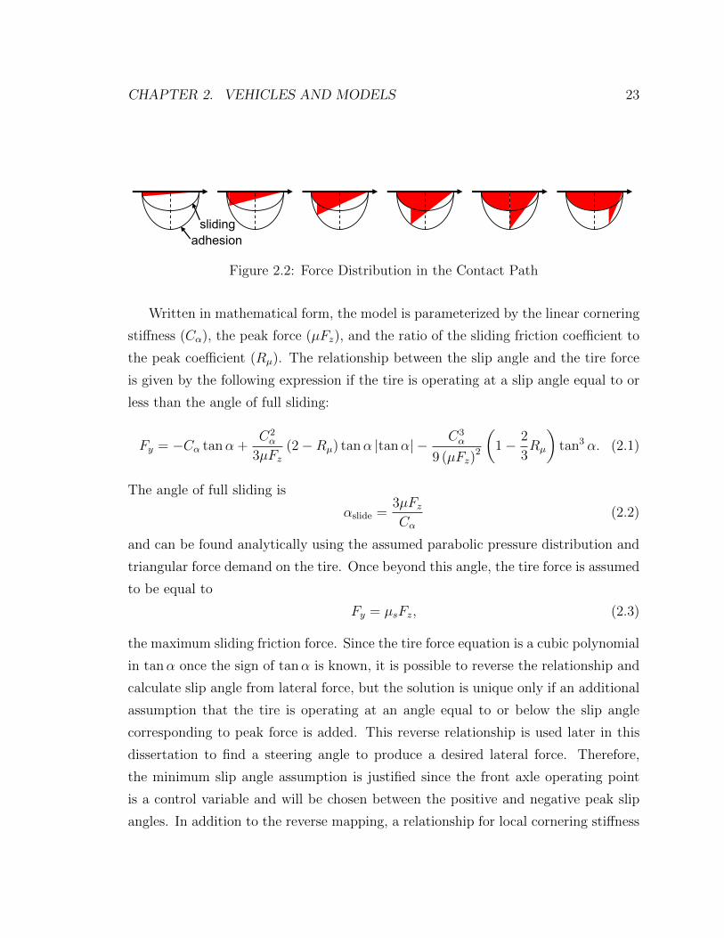
CHAPTER 2. VEHICLES AND MODELS 23
slidingadhesion
Figure 2.2: Force Distribution in the Contact Path
Written in mathematical form, the model is parameterized by the linear cornering
stiffness (Cα), the peak force (µFz), and the ratio of the sliding friction coefficient to
the peak coefficient (Rµ). The relationship between the slip angle and the tire force
is given by the following expression if the tire is operating at a slip angle equal to or
less than the angle of full sliding:
Fy = −Cα tanα +C2
α
3µFz(2−Rµ) tanα |tanα|− C3
α
9 (µFz)2
�1− 2
3Rµ
�tan3 α. (2.1)
The angle of full sliding is
αslide =3µFz
Cα(2.2)
and can be found analytically using the assumed parabolic pressure distribution and
triangular force demand on the tire. Once beyond this angle, the tire force is assumed
to be equal to
Fy = µsFz, (2.3)
the maximum sliding friction force. Since the tire force equation is a cubic polynomial
in tanα once the sign of tanα is known, it is possible to reverse the relationship and
calculate slip angle from lateral force, but the solution is unique only if an additional
assumption that the tire is operating at an angle equal to or below the slip angle
corresponding to peak force is added. This reverse relationship is used later in this
dissertation to find a steering angle to produce a desired lateral force. Therefore,
the minimum slip angle assumption is justified since the front axle operating point
is a control variable and will be chosen between the positive and negative peak slip
angles. In addition to the reverse mapping, a relationship for local cornering stiffness

CHAPTER 2. VEHICLES AND MODELS 24
may be derived from the force model by direct differentiation.
Several explicit relationships also may be derived for a tire at the angle of peak
force generation. The resulting equations (used in developing the control strategy in
the following sections) are:
q =
�1− 2
3Rµ
�−1
(2.4a)
Fypeak = µFz
�−q +
2−Rµ
3q2 −
1− 23Rµ
9q3�
(2.4b)
αpeak = arctan
�qµFz
Cα
�. (2.4c)
where Fypeak is the maximum achievable tire force, and αpeak is the tire slip angle at
which the maximum tire force is attained.
The brush tire model also provides a mechanism for including the effects of lateral-
longitudinal force coupling. In general, the force demand on a tire is a vector sum
of the lateral and longitudinal components and must be less than the total available
force,
Ftot =�F 2x + F 2
y ≤ µFz. (2.5)
A rigorous treatment of this elliptical force limitation on each tire requires that the
rotational dynamics of the tires be modeled. With these rotational dynamics, the
longitudinal slip on the tire can be calculated and the combined slip may be used to
calculate the coupled forces, Fx and Fy, on each axle. Longitudinal slip is defined
as the difference between the free rolling velocity and actual rotational speed of each
wheel, and can be written
κ =ωRw − Vxwheel
Vxwheel
(2.6)
where ω is the wheel rotational speed, Rw is the effective rolling radius, and Vxwheel
is the longitudinal velocity of the wheel center. The longitudinal slip is analogous to
the lateral slip angle of the tire and the two equations for lateral and longitudinal
forces have a common form. Thus, it is possible to combine these equations using the
friction circle concept to yield coupled equations for the lateral and longitudinal tire

CHAPTER 2. VEHICLES AND MODELS 25
Figure 2.3: Combined Tire Force Limits
forces:
γ =
�
C2x
�κ
1 + κ
�2
+ C2α
�tanα
1 + κ
�2
(2.7a)
F =
γ − 1
3µFz
�2− µs
µ
�γ2 + 1
9µ2F 2z
�1− 2µs
3µ
�γ3 γ ≤ 3µFz
µsFz γ > 3µFz
(2.7b)
Fx =Cx
γ
�κ
1 + κ
�F (2.7c)
Fy =−Cα
γ
�tanα
1 + κ
�F. (2.7d)
However, the wheel dynamics are significantly faster than the chassis dynamics
that are pertinent for envelope control. They also add quite a bit of complexity to
the model. Therefore, for the model predictive control problem, an approximation
of this behavior is made by treating the Fx demand as an input that dictates the
maximum available Fy force, as illustrated in Figure 2.3. This “derating” approach
can be expressed as
µFz =�
(µFz)2nom − F 2
x (2.8)
and the adjusted value of µFz can be used as a parameter for the lateral brush tire
model to yield an approximate coupled tire force. For longitudinal forces significantly
smaller than (µFz)nom, this is a relatively good model, but the lack of longitudinal slip

CHAPTER 2. VEHICLES AND MODELS 26
Slip Angle ( )
Tire
For
ce M
agni
tude
Brush Model
C
Linear Model
Figure 2.4: Comparison of Linear and Brush Tire Models
information makes the relationship incomplete. If this method is applied naively with
very large longitudinal forces, the lateral force may be reduced to zero. Therefore,
for use in the envelope control system, µFz is bounded away from zero to improve
the model performance.
2.1.2 Linear Tire Model
For some tasks described in this dissertation, the brush tire model is more detailed
than necessary. At low levels of lateral acceleration with respect to the maximum on
the surface, a linear model describes the tire forces well and provides a useful way to
develop a linear version of bicycle model. The linear tire model yields the following
expressions for the front and rear tire forces,
Fyf = −Cαfαf , Fyr = −Cαrαr (2.9)
where αf and αr are described in terms of the vehicle states and the steering angle
input from the driver.
Despite the complex construction of tires and the influence of stick-slip friction,
their behavior at low levels of lateral force is dominated by the elastic nature of
the rubber. Therefore, this linear model of the tire forces yields good results up to

CHAPTER 2. VEHICLES AND MODELS 27
approximately half of the maximum tire force as seen in Figure 2.4.
2.2 Chassis Models
2.2.1 Four Wheel Yaw-Roll Model
The most complex model of the vehicle dynamics used in this dissertation is repre-
sented in Figure 2.5. The four wheels of the vehicle are connected to each other by
a rigid base, while the body of the vehicle is represented by an inverted pendulum
that rolls about an imaginary axis connecting the front and rear of the vehicle. Ro-
tational states for all four wheels are included, weight transfer between the wheels is
calculated, and the coupled lateral-longitudinal brush tire model is used to calculate
the forces on each tire. The effects of the suspensions are incorporated into the roll
motion of the inverted pendulum and the weight transfer between the wheels, making
this a relatively complete description of the vehicle behavior. The equations for the
yaw, roll, and sideslip derivatives of the vehicle are:
mUx −mrUy +mh�r sinφ+ 2mh�rφ cosφ = Qx (2.10a)
mUy +mrUx −mh�φ cos phi+mh��r2 + φ2
�sinφ = Qy (2.10b)
r =Qψ −Qxh� sinφ− 2 (Iyy − Izz) rφ sinφ cosφ
Iyy sin2 φ+ Izz cos2 φ
(2.10c)
φ =Qyh� cosφ−Kφφ− bφφ+mgh� sinφ+
�(Iyy − Izz) r2 −mh�2φ2
�sinφ cosφ
Ixx +mh�2 sin2 φ
(2.10d)
Qx = (Fxlf + Fxrf ) cos δ − (Fylf + Fyrf ) sin δ + Fxlr + Fxrr (2.10e)
Qy = (Fylf + Fyrf ) cos δ + (Fxlf + Fxrf ) sin δ + Fylr + Fyrr (2.10f)
Qψ = a [(Fylf + Fyrf ) cos δ + (Fxlf + Fxrf ) sin δ]− b [Fylr + Fyrr]
− d2 [(Fxlf − Fxrf ) cos δ − (Fylf − Fyrf ) sin δ + Fxlr − Fxrr]
(2.10g)
where Ixx, Iyy, Izz, are the moments of inertia about the x, y, and z axes, respectively.
Products of inertia are assumed to be zero in this model, though the equations for a

CHAPTER 2. VEHICLES AND MODELS 28
Figure 2.5: Four-wheel Yaw-Roll Model
similar model with non-zero yaw-roll product of inertia may be found in [40].
The four wheel yaw-roll model was used as a virtual testbed to validate the design
of the envelope controller before experiments were performed and provides the basis
for the investigation of vehicle roll control as described in Chapter 6. Perhaps more
importantly, by making certain assumptions about the vehicle state, the four wheel
yaw-roll may be reduced to a variety of other useful and less complicated models.
2.2.2 Bicycle Model
The bicycle model, shown in Figure 2.6, is a two-state model of the vehicle dynamics
that yields a pair of equations that describe the rotational and lateral velocities of the
vehicle. This description of the planar vehicle dynamics is used in the development
of the model predictive envelope controller.
Several key assumptions are made in reducing the yaw-roll model to the bicycle
model. Since the bicycle model is used to describe the planar behavior of the vehicle,
the body roll behavior is neglected by assuming that the mass of the vehicle is entirely

CHAPTER 2. VEHICLES AND MODELS 29
ab
αr
αf
δ
Ux
Uy
r
FyfFyr
Figure 2.6: The Bicycle Model
in the rigid base of the vehicle. Furthermore, for traversing corners of moderate
radius at typical driving speeds, the left and right wheels on each axle attain nearly
identical slip angles. Therefore, the forces from the wheels on each axle are summed
and lumped together as a single equivalent wheel. However, it is well known that
lateral weight transfer and suspension deflections also result in differences between
the left and right wheels. These effects are incorporated into the model through the
use of lumped parameters that are identified from the car in experimental testing.
The cornering stiffness allows the linear tire model to incorporate these effects while
the measured peak force on each axle informs the nonlinear brush tire model.
For the purposes of friction estimation and envelope control, a constant longitu-
dinal velocity is assumed. However, it is noted that accelerating and braking torques
and longitudinal weight transfer play a significant role in determining the lateral be-
havior of the vehicle. Fortunately, these influences on the lateral tire forces may
be approximated separately and are included where necessary to achieve sufficient
accuracy in the lateral dynamics.
The equations of motion for the bicycle model are developed from first principles
by writing a force balance in the vehicle y-coordinate and a moment balance around
the z-axis, also known as the yaw axis.
may = Fyf + Fyr, rIzz = aFyf − bFyr (2.11)

CHAPTER 2. VEHICLES AND MODELS 30
The lateral acceleration of the vehicle in an inertial reference frame is
ay = Uy + rUx (2.12)
and small angles are assumed to obtain a linear approximation for the sideslip angle
β = tan−1
�Uy
Ux
�to β =
Uy
Ux. (2.13)
Using these expressions for lateral acceleration and sideslip angle, Eq. 2.11 can be
rearranged to find state equations for the sideslip angle and yaw rate:
m�Uy + rUx
�= Fyf + Fyr rIzz = aFyf − bFyr (2.14)
β =Fyf + Fyr
mUx− r r =
aFyf − bFyr
Izz(2.15)
where the parameters m and Izz are the vehicle mass and yaw moment of inertia,
respectively.
The forces, Fyf and Fyr, are generated by the tires at each axle and are highly
nonlinear at elevated levels of lateral acceleration. Therefore, the nonlinear brush
model may be used to describe their force generating characteristics. However, at
low levels of lateral acceleration, the linear model describes the tire forces well and
provides a useful way to develop a completely linear version of bicycle model. Like
the sideslip angle of the vehicle, small angles are assumed to get linear expressions
for the axle slip angles:
αf = β +ar
Ux− δ, αr = β − br
Ux. (2.16)
The driver input, δ, is also included through these slip angle expressions. Substitution
of these slip angles into the linear tire force equations (Eq. 2.9) and then into the state
equations in Eq. 2.15 yields a pair of differential equations that specify the behavior
of the two states when the driver input is known. This system can be written in
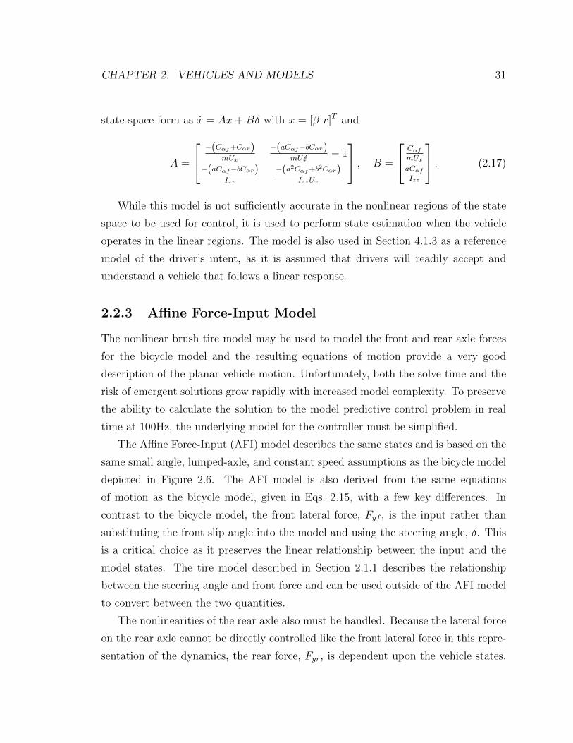
CHAPTER 2. VEHICLES AND MODELS 31
state-space form as x = Ax+Bδ with x = [β r]T and
A =
−(Cαf+Cαr)
mUx
−(aCαf−bCαr)mU2
x− 1
−(aCαf−bCαr)Izz
−(a2Cαf+b2Cαr)IzzUx
, B =
Cαf
mUx
aCαf
Izz
. (2.17)
While this model is not sufficiently accurate in the nonlinear regions of the state
space to be used for control, it is used to perform state estimation when the vehicle
operates in the linear regions. The model is also used in Section 4.1.3 as a reference
model of the driver’s intent, as it is assumed that drivers will readily accept and
understand a vehicle that follows a linear response.
2.2.3 Affine Force-Input Model
The nonlinear brush tire model may be used to model the front and rear axle forces
for the bicycle model and the resulting equations of motion provide a very good
description of the planar vehicle motion. Unfortunately, both the solve time and the
risk of emergent solutions grow rapidly with increased model complexity. To preserve
the ability to calculate the solution to the model predictive control problem in real
time at 100Hz, the underlying model for the controller must be simplified.
The Affine Force-Input (AFI) model describes the same states and is based on the
same small angle, lumped-axle, and constant speed assumptions as the bicycle model
depicted in Figure 2.6. The AFI model is also derived from the same equations
of motion as the bicycle model, given in Eqs. 2.15, with a few key differences. In
contrast to the bicycle model, the front lateral force, Fyf , is the input rather than
substituting the front slip angle into the model and using the steering angle, δ. This
is a critical choice as it preserves the linear relationship between the input and the
model states. The tire model described in Section 2.1.1 describes the relationship
between the steering angle and front force and can be used outside of the AFI model
to convert between the two quantities.
The nonlinearities of the rear axle also must be handled. Because the lateral force
on the rear axle cannot be directly controlled like the front lateral force in this repre-
sentation of the dynamics, the rear force, Fyr, is dependent upon the vehicle states.

CHAPTER 2. VEHICLES AND MODELS 32
Therefore, to represent the link between the vehicle motion and the rear tire force,
the brush tire model is linearized about the slip angle operating point. This lineariza-
tion is found by taking the zeroth and first-order terms of the Taylor expansion of a
smooth tire model, from which the tire force, F yr and the local cornering stiffness,�Cαr can be found at the operating point, αr.
Fyr = F yr − �Cαr (αr − αr) (2.18)
This rear tire force equation is affine in the rear slip angle αr, which provides a
representation of the saturation behavior of the tire without including a nonlinear
expression. Substituting Eq. 2.18 into Eq. 2.15 yields:
β =Fyf + F yr − �Cαr (αr − αr)
mUx− r (2.19a)
r =aFyf − b
�F yr − �Cαr (αr − αr)
�
Izz. (2.19b)
Like the bicycle model, small angle assumptions allow the rear slip angle to be written
αr = β − bUxr, which yields
β =Fyf + F yr − �Cαr
�β − b
Uxr − αr
�
mUx− r (2.20a)
r =aFyf − b
�F yr − �Cαr
�β − b
Uxr − αr
��
Izz. (2.20b)
A state-space description of the system needed for use in the model predictive control
problem can be defined as x = Ax+BFyf + d, where again x = [β r]T with
A =
− �Cαr
mUx
b �CαrmU2
x− 1
b �CαrIzz
− b2 �CαrUxIzz
, B =
1
mUx
aIzz
, d =
(F yr+ �Cαrαr)
mUx
−b(F yr+ �Cαrαr)Izz
. (2.21)
The resulting model satisfies the requirements for convexity and allows for the use of
efficient optimization techniques when implementing the model predictive controller.

CHAPTER 2. VEHICLES AND MODELS 33
2.2.4 Linearized Roll Model
When extending the model predictive envelope controller to control vehicle roll, there
is no direct actuation of the roll states and any roll motion is excited solely by the
planar motion of the vehicle. Therefore, it is critical for the model to describe the
planar dynamics as well as the mechanism for transferring energy into the roll modes
of the vehicle. At the same time, the model must be simple enough to underly a
model predictive control scheme.
The compromise between modeling complexity and solve speed for the MPC prob-
lem is handled by linearizing the equations of motion for the yaw roll model, neglecting
the rotational dynamics of the wheels, and utilizing a linear model to produce the
tire forces. All four wheels are included for the purposes of incorporating differential
drive, but the lateral forces are calculated with a common axle slip angle for the
left and right wheels. As with the other models, small angles and a constant vehicle
velocity are assumed.
The state variables selected to represent the base mode of the vehicle are the yaw
rate about the body pivot point and the vehicle slip angle between the vehicle velocity
at the pivot point and the vehicle heading. For the roll mode, the states are the angle
and rotation rate of the pendulum about the pivot point. There are also three inputs
to the model: front steering angle, rear steering angle, and rear differential drive. The
roll controller presented later in this dissertation takes advantage of these multiple
actuators to achieve the desired vehicle states. To incorporate the rear wheel steering,
the rear slip angle is redefined to include the extra input:
αr =Uy − ra
Ux− δr. (2.22)
Rear wheel differential drive may be generated by modulating the engine of a rear-
wheel-drive car or the rear brake channels of a vehicle with ABS/stability control.
Therefore, these inputs are represented by two longitudinal force terms in the yaw
equation.
Combining these inputs with the nonlinear yaw-roll equations and linearizing, the

CHAPTER 2. VEHICLES AND MODELS 34
model can be described by the following equations:
Fyf + Fyr = ms
�Ux
�β + r
�− hφ
�+muUx
�β + r
�(2.23a)
aFyf − bFyr +d
2(Fxr − Fxl) = Izz r (2.23b)
(msgh−Kφ)φ− bφφ+msh�Ux
�β + r
�− hφ
�= Ixxφ (2.23c)
As with the planar envelope control problem, a computationally efficient model is
needed for the optimization phase of the model predictive control step. Therefore, for
the roll control task, the linear tire model was selected in order phrase the problem as
a quadratic program (QP), a specific type of convex optimization problem that may
be solved rapidly and robustly.
The linearized equations can be rearranged to obtain the continuous time state
space representation of the system that is discretized and used in the roll control
investigation.
β
r
φ
φ
=
−IeqC0
mU2xIcomb
−Ieq[C1+mU2x]
mU2xIcomb
+ m2sh
2Ux
mUxIcomb
msh(msgh−Kφ)mUxIcomb
−mshbφmUxIcomb
−C1IzzUx
−C2IzzUx
0 0
0 0 0 1
−mshC0mUxIcomb
−msh[C1+mU2x]
mUxIcomb+ mshUx
Icomb
(msgh−Kφ)Icomb
−bφIcomb
β
r
φ
φ
+
Cαf IeqmUxIcomb
0 0aCαf
Izzd
2Izz− d
2Izz
0 0 0mshCαf
mIcomb0 0
δf
Fxlr
Fxrr
(2.24)
2.2.5 Summary of Models
Table 2.1 summarizes the key features of the models that were introduced in the
previous subsections.

CHAPTER 2. VEHICLES AND MODELS 35
Table 2.1: Vehicle Models
Chassis Model Tire Model Assumptions
Four wheel yaw-roll Coupled brush Vehicle body as inverted pendulum
Bicycle Linear No roll, small angles,
lumped wheels, constant speed
Affine Force Input Lateral brush No roll, small angles,
lumped wheels, constant speed
Linearized roll Linear Pendulum body, small angles,
constant speed
2.3 P1 By-Wire Test Vehicle
The parameters used for the models described in the previous section are those of
an experimental test vehicle constructed by students at Stanford University. This
vehicle, referred to as P1 and shown in Figure 2.7, is a rear-wheel drive vehicle
powered by independent left and right electric drive motors. P1 is also equipped
with a pair of GPS systems that provide velocity and attitude information that is
fused with inertial measurements to achieve high-accuracy full-state feedback at a
500Hz update rate, as described in [57]. The steering system includes independent
left- and right-wheel actuation with high bandwidth response, as detailed in [40], and
the handling properties of P1 are consistent with those of a sports sedan – with one
important exception – and are detailed in Table 2.2.
The exception to the normal handling properties for P1 is the yaw moment of
inertia. Compared to the mass, wheelbase, and track width, the moment of inertia is
unusually small. In addition, the drive system of P1 provides regenerative braking on
the rear axle when the driver lifts off the accelerator pedal. The combination of these
properties results in the vehicle being highly sensitive to accelerator inputs by the
driver while cornering. In open-loop driving with the vehicle on a low-friction surface,
drivers are often unable to stabilize the vehicle in drive-torque induced oversteer.

CHAPTER 2. VEHICLES AND MODELS 36
Figure 2.7: P1 Steer and Drive By-Wire Research Testbed
Table 2.2: Parameters for the P1 test vehicle
Parameter Symbol Value Units
vehicle mass m 1724 kg
yaw moment-of-inertia Izz 1100 kgm2
wheelbase L 2.5 m
front axle-CG distance a 1.35 m
rear axle-CG distance b 1.15 m
front cornering stiffness Cαf90000 N
rad
rear cornering stiffness Cαr 138000 Nrad
CHAPTER 2. VEHICLES AND MODELS 37
2.4 Experimental Testing
For the experimental validation given in later chapters of this dissertation, tests were
performed on surfaces comprised of mixed dirt, gravel, and asphalt. The friction
characteristics of the surfaces were therefore highly variable. Some sections with very
little loose dirt and gravel had normal adhesive friction characteristics of asphalt while
other sections with a lot of gravel would allow the tires to slide quite a bit. The varia-
tion in the distribution of loose particles on the surface was estimated to have a length
scale on the order of tens of centimeters and at speed, an average friction coefficient
of 0.6 was a suitable estimate. In some experiments, the friction information, as well
as the sideslip angle, were estimated in real time using the technique described in [32],
but for many of the initial experiments with the controller, a static a priori estimate
of the friction properties and GPS-based state estimation were used to isolate the
controller behavior from any undesired estimator-controller interactions.

Chapter 3
Vehicle Instability
While it is well known that a vehicle may become unstable once it reaches certain
states in the nonlinear regions of the tires, there has been little published previously to
describe the transition of the vehicle from normal driving into the unstable handling
regime. This chapter presents an analysis of the driving dynamics and demonstrates
the appearance of unstable dynamics across a range of vehicles, speeds, and driver
inputs.
3.1 Instability Dynamics
Using a two-state model, it is possible to develop phase plane representations of the
vehicle dynamics in the linear and nonlinear handling regimes. These plots allow the
designer of a driver assistance system to identify regions in which the dynamics are
unfavorable and in which the vehicle would fail to respond in a manner that most
drivers would expect. These are the regions in which production stability control
systems activate to assist the driver. A driver assistance system based on handling
envelopes would seek to prevent the vehicle from entering these regions at all.
The phase plots shown in this dissertation are “snapshots” of the dynamics of
the vehicle model at various conditions. To obtain a reasonable level of accuracy,
the dynamics are calculated from a bicycle model with nonlinear tires and no small
angle assumptions. The sideslip and yaw rate states of the vehicle are plotted on the
38
CHAPTER 3. VEHICLE INSTABILITY 39
horizontal and vertical axes, respectively. Since only two variables can be represented
in these plots, all other vehicle parameters are held constant. Therefore, each plot
shows the vehicle dynamics at a specific friction coefficient, vehicle speed, and driver
steering angle. Inagaki, et. al. examined this yaw-sideslip plane but argued in favor
of a plane with the sideslip derivative plotted against sideslip due to the location and
movement of the equilibria [62]. Hoffman, et. al. utilized a similar analysis where a
simulated closed loop maneuver was plotted over a three-dimensional envelope in the
open loop β − β − δ space [30].
The first set of phase plots shown in this section illustrates the dynamics of a
vehicle being driven at 10ms on a surface with an average coefficient of friction of 0.6.
The parameters for the vehicle are those of the P1 test vehicle, seen in Figure 2.7.
This vehicle is mildly understeering in the linear region, with an understeer gradient
of 0.02 radg . At the handling limits, the vehicle is close to being neutral, but tends
slightly to limit oversteering. The driver steering input in the set of plots progresses
from 3◦ at the road wheels in Figure 3.1a up to 12◦ in Figure 3.1d.
For each phase plot in Figures 3.1a-3.1c, there are three equilibria. In these plots,
the steering angles are less than or equal to 10◦ and there is a stable equilibrium
on each plot at moderate yaw rate and sideslip angles. There are also two saddle
points that separate regions of stable handling from unstable regions. These saddle
points are located along lines of constant yaw rate, in this case at approximately
0.59 radg . As the steering angle of the vehicle is increased, the stable equilibria of
the vehicle move to higher yaw rates and larger (negative) sideslip angles, while the
regions of instability shift, as seen by the movement of the saddle points toward lower
sideslip angles. Figure 3.1d illustrates the vehicle behavior when the steering angle
is increased to 12◦. At this steering angle, the vehicle is unstable, as evidenced by a
bifurcation from a stable to unstable equilibrium. Nearly all trajectories of the system
result in the growth of the vehicle yaw rate followed by the vehicle sliding sideways
with a large sideslip angle. Since the vehicle is nearly neutral steering, the yaw rate
remains moderate during the slide.
These plots yield interesting insights for the design of stability controllers. Even
though Figures 3.1a-3.1c show vehicle behaviors with stable dynamics immediately

CHAPTER 3. VEHICLE INSTABILITY 40
5 4 3 2 1 1 2 3 4 5
8
6
4
2
2
4
6
8
Sideslip Angle (rad)
Yaw Rate (rad/s)
(a) 3 degrees Steering Angle
5 4 3 2 1 1 2 3 4 5
8
6
4
2
2
4
6
8
Sideslip Angle (rad)
Yaw Rate (rad/s)
(b) 7 degrees Steering Angle
5 4 3 2 1 1 2 3 4 5
8
6
4
2
2
4
6
8
Sideslip Angle (rad)
Yaw Rate (rad/s)
(c) 10 degrees Steering Angle
5 4 3 2 1 1 2 3 4 5
8
6
4
2
2
4
6
8
Sideslip Angle (rad)
Yaw Rate (rad/s)
(d) 12 degrees steering angle
Figure 3.1: Neutral Vehicle Dynamics at 10m/s with 0.6 Surface Friction Coefficient
surrounding the equilibria, unstable regions exist for all of these conditions. Therefore,
a stability control system should seek to prevent the vehicle from entering these
regions in case of disturbances to the system. Fortunately, the unstable dynamics
occur in the same location, regardless of the driver’s steering input. The dotted black
line on each of the phase plots in Figure 3.1d represents the maximum equilibrium
yaw rate for the vehicle. This yaw rate may be found utilizing the maximum tire

CHAPTER 3. VEHICLE INSTABILITY 41
force at each axle. The yaw rate is in equilibrium when
r =aFyf − bFyr
Izz= 0 (3.1)
Fyf =b
aFyr, (3.2)
assuming that lateral aerodynamic forces can be neglected in the driving conditions
considered in this dissertation.
With the simplified model of the lateral vehicle dynamics used in this investigation,
each tire simultaneously reaches its maximum force at steady state. However, other
effects such as weight transfer, suspension motions, and drive torque can cause one
axle to reach saturation earlier than the other. If this occurs, one axle will limit the
maximum yaw rate. If Fyfmax ≤ baFyrmax , then the equilibrium is dictated by the front
lateral tire force. If Fyfmax ≥ baFyrmax , then the rear lateral tire force dictates the
equilibrium. If the driver has pushed the vehicle to the equilibrium associated with
the limiting tire force, then β = 0 and
r =
Fyrmax (1+b/a)mUx
Fyfmax ≥ baFyrmax
Fyfmax (1+a/b)mUx
Fyfmax <baFyrmax
(3.3)
Therefore, this line of constant yaw rate separates the areas of convergent sideslip
dynamics from the areas of divergent dynamics. Furthermore, examining Figure 3.1d,
when the driver steers far enough to cause the vehicle to slide without any external
disturbance, the vehicle yaw rate grows rapidly with low sideslip angles prior to
exceeding the equilibrium yaw rate and developing large sideslip. This observation
also makes clear the underlying reason for the efficacy of stability control through
independent braking to produce a yaw moment, or what many authors term Direct
Yaw Control (DYC) [43, 41]. By restricting the yaw rate from deviating significantly
from a linear reference, large growth in vehicle sideslip angle can be prevented, even
when direct measurements of sideslip angle are absent.
While the handling properties of the vehicle used for the phase plots in Figure 3.1
are quite neutral at the limits of handling, the observations made about the regions of

CHAPTER 3. VEHICLE INSTABILITY 42
5 4 3 2 1 1 2 3 4 5
8
6
4
2
2
4
6
8
Sideslip Angle (rad)
Yaw
Rat
e (ra
d/s)
(a) 3 degrees Steering Angle
5 4 3 2 1 1 2 3 4 5
8
6
4
2
2
4
6
8
Sideslip Angle
Yaw
Rat
e
(b) 7 degrees Steering Angle
5 4 3 2 1 1 2 3 4 5
8
6
4
2
2
4
6
8
Sideslip Angle
Yaw
Rat
e
(c) 10 degrees Steering Angle
5 4 3 2 1 1 2 3 4 5
8
6
4
2
2
4
6
8
Sideslip Angle (rad)
Yaw
Rat
e (ra
d/s)
a
(d) 12 degrees Steering Angle
Figure 3.2: Understeering Vehicle Dynamics at 10m/s
instability remain valid for understeering and oversteering vehicles as well. Not only
is this important for evaluating production vehicles with different weight distributions
and handling properties, but it is also critical since the application of drive and brake
torques can alter the handling behavior at the friction limits. Figure 3.2 shows the
same vehicle as before, but with the maximum available force on the front axle reduced
to produce limit understeering behavior. Figure 3.3 illustrates the same vehicle again,
but with the friction on the rear axle reduced to produce limit oversteering behavior.
In each case, the axle with reduced force capability is modeled with an effective
friction coefficient of 0.55, reduced from 0.6.

CHAPTER 3. VEHICLE INSTABILITY 43
5 4 3 2 1 1 2 3 4 5
8
6
4
2
2
4
6
8
Sideslip Angle (rad)
Yaw
Rat
e (ra
d/s)
(a) 3 degrees Steering Angle
5 4 3 2 1 1 2 3 4 5
8
6
4
2
2
4
6
8
Sideslip Angle
Yaw
Rat
e
(b) 7 degrees Steering Angle
5 4 3 2 1 1 2 3 4 5
8
6
4
2
2
4
6
8
Sideslip Angle
Yaw
Rat
e
(c) 10 degrees Steering Angle
5 4 3 2 1 1 2 3 4 5
8
6
4
2
2
4
6
8
Sideslip Angle (rad)
Yaw
Rat
e (ra
d/s)
(d) 12 degrees Steering Angle
Figure 3.3: Oversteering Vehicle Dynamics at 10m/s
When the vehicle understeers, the stability problems of the neutral vehicle disap-
pear, but the oscillatory behavior associated with an understeering vehicle becomes
apparent. Like the neutral vehicle, there is also convergence to the equilibria within
the maximum yaw equilibrium bounds. The oversteering vehicle, as expected, demon-
strates significant degradation of stability. For 7◦ of steering angle, the stable equi-
librium is quite close to the saddle point, beyond which the dynamics are strongly
divergent. As a result, minor disturbances at this condition could cause the vehicle
to spin. When the steering angle is increased to 10◦, the vehicle exhibits the unstable
tendencies seen at larger steering angles with the neutral steering vehicle. However, in

CHAPTER 3. VEHICLE INSTABILITY 44
Yaw
Rat
e (ra
d/s)
Sideslip Angle (rad)
Figure 3.4: Vehicle Dynamics at 10m/s on Slippery Surface with Large Steer Angle
this case, the yaw rate continues to grow once the maximum equilibrium boundaries
are exceeded and the vehicle “spins out” rather than experiencing a lateral slide.
This can be seen in experimental data as well. P1, the experimental steer-by-wire
testbed for which the parameter set was taken for the plots in Figure 3.1, was used
to perform an experiment where the vehicle was driven manually to equilibrium cor-
nering. At 10ms and at an equilibrium near 0.4 rad
g yaw rate, the accelerator pedal was
used to upset the vehicle in the corner, yielding dynamics somewhere in between the
neutral nominal dynamics and the oversteering dynamics illustrated in the previous
plots. No controller was active on the vehicle during the test, and the steering angle
was held constant. Figure 3.4 shows the state trajectory of the vehicle in the phase
plane. From this plot, the behavior that is expected from the phase plane analysis is
evident. Because the vehicle is upset with rear wheel torque, the initial phase of the
maneuver approximately follows the unstable growth of yaw rate seen in Figure 3.3
as a result of reduced lateral force capability on the rear axle. Once the vehicle is
upset, the accelerator is released and the neutral steering characteristics of the vehicle
return. However, since the yaw rate is well into the region of unfavorable dynamics,

CHAPTER 3. VEHICLE INSTABILITY 45
5 4 3 2 1 1 2 3 4 5
8
6
4
2
2
4
6
8
Sideslip Angle
Yaw
Rat
e
Figure 3.5: Neutral Vehicle Dynamics at 15m/s with 7 degrees Steering and 0.6Surface Friction Coefficient
the sideslip angle grows rapidly as the vehicle spins, as is predicted by the upper
left hand portion of the phase plots in Figure 3.1. The experimental data from the
maneuver are truncated for clarity, but the vehicle comes to rest at a sideslip angle
of over 180◦ as it fully spins out.
Aside from the steering angle from the driver, the vehicle speed is also a critical
parameter. From the expression of the lateral acceleration, ay = β + rUx, it is clear
that since the forces needed to produce lateral acceleration are limited, as the vehicle
speed increases, the maximum yaw rate must decrease. Figure 3.5 shows the phase
plane for the vehicle with a 7◦ driver steering angle on the same surface as the previous
figures, but at 15ms . While the lines of maximum steady state yaw rate are located
at lower values and the steering angle that destabilizes the vehicle is smaller, the
dynamics are remarkably similar to those illustrated in Figure 3.1d. In both plots,
the unstable dynamics occur in the same location relative to the lines of maximum
yaw equilibrium.
From the plots shown in this section, it is clear that regions of unstable dynamics

CHAPTER 3. VEHICLE INSTABILITY 46
can be identified and separated from the stable regions of handling by a constant
yaw rate boundary. All of the stable equilibria for the bicycle model lie within these
bounds, and the work of Hindiyeh and Gerdes [28] demonstrates that even the equi-
libria for high sideslip “drifting” maneuvers lie along these bounds. Supporting the
importance of measuring and bounding the yaw rate of a vehicle is the observation
that over the range of steering angles, speeds, and vehicle handling properties, the
large sideslip angles develop only after the yaw rate grows large. Since this yaw
measurement can be made directly, accurately, and inexpensively, these observations
suggest excellent opportunities for control.
3.2 Defining Boundaries of Unstable Regions
In designing a stability controller, the objective is to assist the driver in maintaining,
to the extent that the dynamics allow, control over the orientation and path of the
vehicle. In the best case, the system would allow the driver to have full authority
over the vehicle in all situations in which the vehicle dynamics are favorable and
intervene only in the case of the vehicle beginning to enter a region of unstable
dynamics. Therefore, the insights gained from the yaw-sideslip phase plane in the
previous section can be used to develop an envelope that includes a large set of
the stable dynamics but excludes regions of instability. Since there are well-defined
undesirable regions, the primary challenge in determining the envelope is thus to
calculate the boundaries of an appropriate envelope in real time.
Fortunately, many vehicles being manufactured today are incorporating electric
power steering and future vehicles may be equipped with steer-by-wire, both of which
have been shown by Hsu and Gerdes [32] to allow for estimates of both sideslip angle
and tire-road friction coefficient. It is this additional information that enables the
identification of stable handling envelopes.

CHAPTER 3. VEHICLE INSTABILITY 47
3.2.1 Defining a Safe Handling Envelope
In the previous section, analysis of the unstable vehicle dynamics showed that the
equilibrium yaw rate associated with the maximum available tire forces is a key quan-
tity. Below this yaw rate, the vehicle dynamics are stable and the states converge
toward stable equilibria. Therefore, it makes sense when designing a stable handling
region to include a yaw rate constraint. Assuming that the axle normal loads are
known and the tire-road friction coefficient can be estimated with a technique such as
that presented by Hsu and Gerdes, then a tire model may be assumed and a yaw rate
constraint can be expressed simply as a function of the estimated peak tire forces:
rmax =
Fyrmax (1+b/a)mUx
Fyfmax ≥ baFyrmax
Fyfmax (1+a/b)mUx
Fyfmax <baFyrmax
(3.4)
This yaw rate constraint is, however, not sufficient to completely ensure the stabil-
ity of the vehicle. In certain low-friction conditions, it is possible for disturbances or
transients to excite large sideslip angles while maintaining low yaw rates, as demon-
strated by Rock, et. al. [56]. To prevent the vehicle from reaching this condition,
a second set of bounds can be used to close the stable handling envelope. A variety
of boundaries may be chosen for this purpose, but choosing a constraint on the rear
axle slip angle results in natural scaling of the envelope. This is in part due to the
fact that the rear slip angle remains small at low speeds and does not exhibit the
non-minimum phase behavior seen in the sideslip angle. The rear slip angle is also a
linear combination of the vehicle sideslip angle and the yaw rate and is dependent on
the vehicle speed, as seen by the rear slip expression, αr = β − bUxr.
As a result, the allowed sideslip scales naturally with both the speed and the yaw
rate, allowing the driver to utilize a significant portion of the state space associated
with stable driving. One natural choice for the value of this rear slip angle boundary
is the angle at which the tire force reaches full saturation. Thus, a controller that
enforces these boundaries will maintain the vehicle within the grip limits of the tires.
However, choosing the rear slip limit in this way may feel constraining to skilled
drivers who may be capable of driving the vehicle with the rear tires in saturation.

CHAPTER 3. VEHICLE INSTABILITY 48
5 4 3 2 1 1 2 3 4 5
8
6
4
2
2
4
6
8
Sideslip Angle (rad)
Yaw
Rat
e (ra
d/s)
Figure 3.6: Phase Portrait with Model Predictive Envelope Controller
Fortunately, arbitrarily wide rear slip limits may be chosen to allow skilled drivers to
drift the vehicle without a stability control intervention and yet vehicle stability can
be guaranteed.
The envelope boundaries form a parallelogram in the yaw-sideslip plane, as illus-
trated in Figure 3.6, where the stable handling envelope is plotted over the phase plane
with a model predictive envelope controller active. From this figure, it is clear that
the dynamics on the interior of the envelope are nearly identical to the uncontrolled
vehicle. However, outside the envelope, the controller alters the unstable dynamics to
stabilize the unstable regions and push the vehicle back toward the envelope interior.
The remaining task is to verify that it is possible to design a controller to enforce
the invariance of the envelope. This is done by finding a control input that causes
the yaw rate and sideslip derivatives to cut into the envelope on every portion of the
boundary.
If active front steering is used to enforce the boundaries of the envelope, the control
action on the boundary is to alter the front axle lateral force. Figure 3.7 shows the
envelope with possible state derivatives plotted at points on each of the boundaries.

CHAPTER 3. VEHICLE INSTABILITY 49
−0.2 −0.15 −0.1 −0.05 0 0.05 0.1 0.15 0.2−0.8
−0.6
−0.4
−0.2
0
0.2
0.4
0.6
0.8
Sideslip Angle (rad)
Yaw
Rat
e (ra
d/s)
Figure 3.7: Ranges of Possible Vehicle Trajectories on Envelope Boundaries
The set of arrows at each point shows the complete range from the minimum to the
maximum front lateral force. From the diagram, it is possible to see that at every
point, there is a trajectory that stays within the envelope. At the top right and bottom
left corners, only the extreme lateral force keeps the vehicle in the envelope. However,
this is sufficient to establish the feasibility of creating an invariant envelope. More
complete statements are presented for the model predictive envelope controller in the
following chapter. Similar analyses may be performed for other actuation schemes,
including independent braking such as that used by production stability control, rear
wheel steering, or differential drive.
3.2.2 Alternative Envelopes
In defining a safe handling envelope, there are a variety of choices that may be made.
The envelope presented in the previous section is straightforward to develop, analyze,
and implement. Chapter 4 will demonstrate that this envelope is also capable of
the desired augmentation of the vehicle dynamics in cooperation with the driver.

CHAPTER 3. VEHICLE INSTABILITY 50
However, there are a number of other envelopes that may be utilized instead. This
section presents several alternative envelope formulations.
An Envelope to Allow Rear Tire Sliding
As mentioned in the description of the envelope in the previous section, it is possible
to change the value of the rear slip angle bounds. This does not result in a change in
the shape of the envelope, but merely makes the envelope wider. This larger envelope
allows a driver to fully saturate the rear tires, as is done in drifting, and the controller
only intervenes if the driver fails to keep the vehicle within these wider bounds.
Since these boundaries are designed to allow skilled drivers to maximize the capa-
bilities of the vehicle, it is also interesting to see how the same system might be viewed
by a less skilled driver. Assuming that the less skilled driver intends to maintain rear
tire grip, any excursion beyond the peak slip angle can be viewed as a mistake. If
this happens and the driver fails to correct, the rear end of the car will slide up until
the point where the envelope controller intervenes. With the rear slip angle bounds
set at this wider point, this motion will be felt by the driver, allowing the driver to
experience and learn from these dynamics without losing control of the car.
Figure 3.8 illustrates the dynamics of the vehicle under envelope control with yaw
rate bounds as described in the previous section, but with wider slip angle boundaries
set at ±20◦. The vehicle speed and steering angle are 10ms and 10◦, respectively. The
action of the controller is similar to that of the narrow boundary controller, where
the dynamics on the interior of the envelope remain very similar to the uncontrolled
vehicle. However, above the yaw rate boundary, the controller intervenes strongly to
prevent the buildup of excessive yaw rate and sideslip angle such as in the uncontrolled
case.
An Envelope to Allow more “Turn-in”
Skilled drivers, particularly those with racing experience, may notice with both the
narrow and wide boundary envelopes presented in the previous sections that the
yaw response when initiating a corner is slightly diminished when compared to the

CHAPTER 3. VEHICLE INSTABILITY 51
5 4 3 2 1 1 2 3 4 5
8
6
4
2
2
4
6
8
Sideslip Angle (rad)
Yaw
Rat
e (ra
d/s)
Figure 3.8: Handling Envelope for 10◦ Steering at 10ms with Slip Bounds at ±20◦
uncontrolled vehicle. This is because the yaw response of the uncontrolled system
has a small overshoot in the yaw rate before reaching equilibrium. This can be
seen in Figure 3.9c. In order to restore this turn-in response, the constant yaw rate
boundary can be changed to a graduated yaw boundary that allows for more yaw
rate at low sideslip angles. This variation of the yaw rate boundary is shown in
Figures 3.9a and 3.9b. The yaw boundary is set so that it passes through the rear
tire slip angle for peak force at the maximum steady state yaw rate. The slope of the
line is then set by choosing the amount of additional yaw rate to allow at zero sideslip
angle. In Figure 3.9, this is set to 15%. Because of a convexity requirement for the
envelope and the fixed point for the boundary to pass through, this forces a slight
reduction in the allowed rear slip angle at higher yaw rates, as seen in Figure 3.9a.
Thus, the additional allowed “turn-in” yaw rate and slip angle at higher yaw rates
are traded off, and the designer of the system must select the best compromise for
the driving style of intended drivers.
One final advantage to this approach is that if the boundary is chosen prop-
erly, the controller need not interfere with the normal stable dynamics, even when
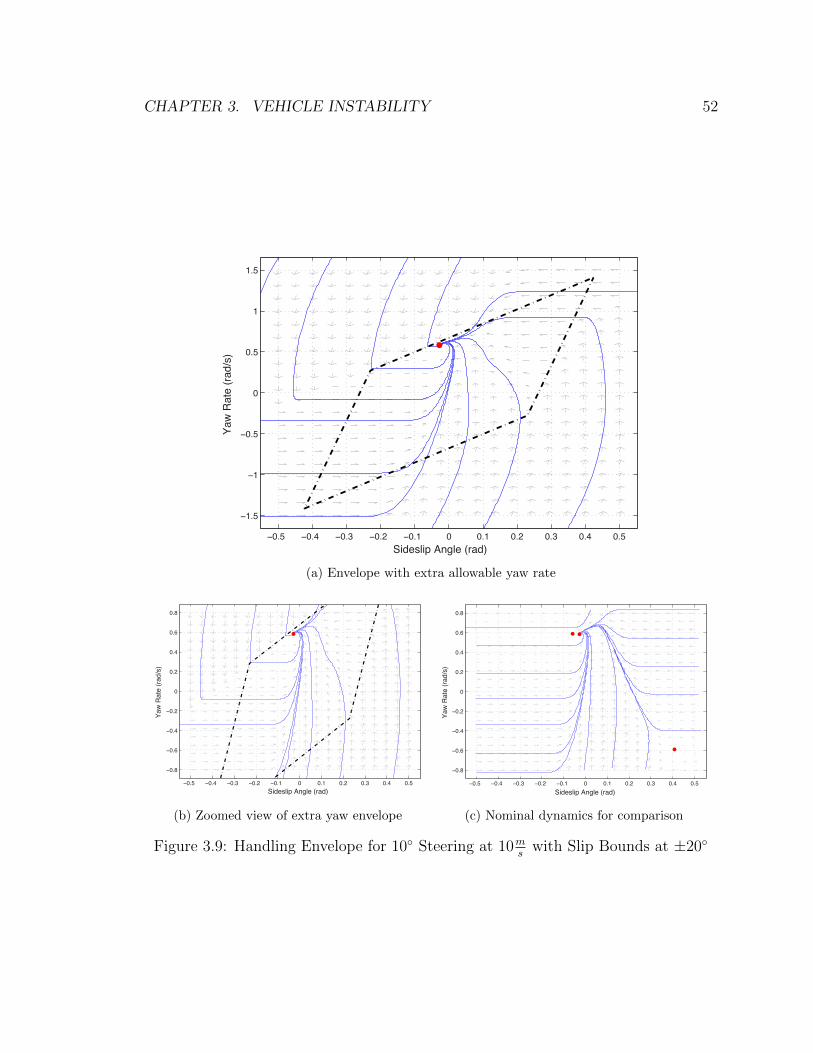
CHAPTER 3. VEHICLE INSTABILITY 52
5 4 3 2 1 1 2 3 4 5
5
5
5
1
5
Sideslip Angle (rad)
Yaw
Rat
e (ra
d/s)
(a) Envelope with extra allowable yaw rate
5 4 3 2 1 1 2 3 4 5
8
6
4
2
2
4
6
8
Sideslip Angle (rad)
Yaw
Rat
e (ra
d/s)
(b) Zoomed view of extra yaw envelope
5 4 3 2 1 1 2 3 4 5
8
6
4
2
2
4
6
8
Sideslip Angle (rad)
Yaw
Rat
e (ra
d/s)
(c) Nominal dynamics for comparison
Figure 3.9: Handling Envelope for 10◦ Steering at 10ms with Slip Bounds at ±20◦
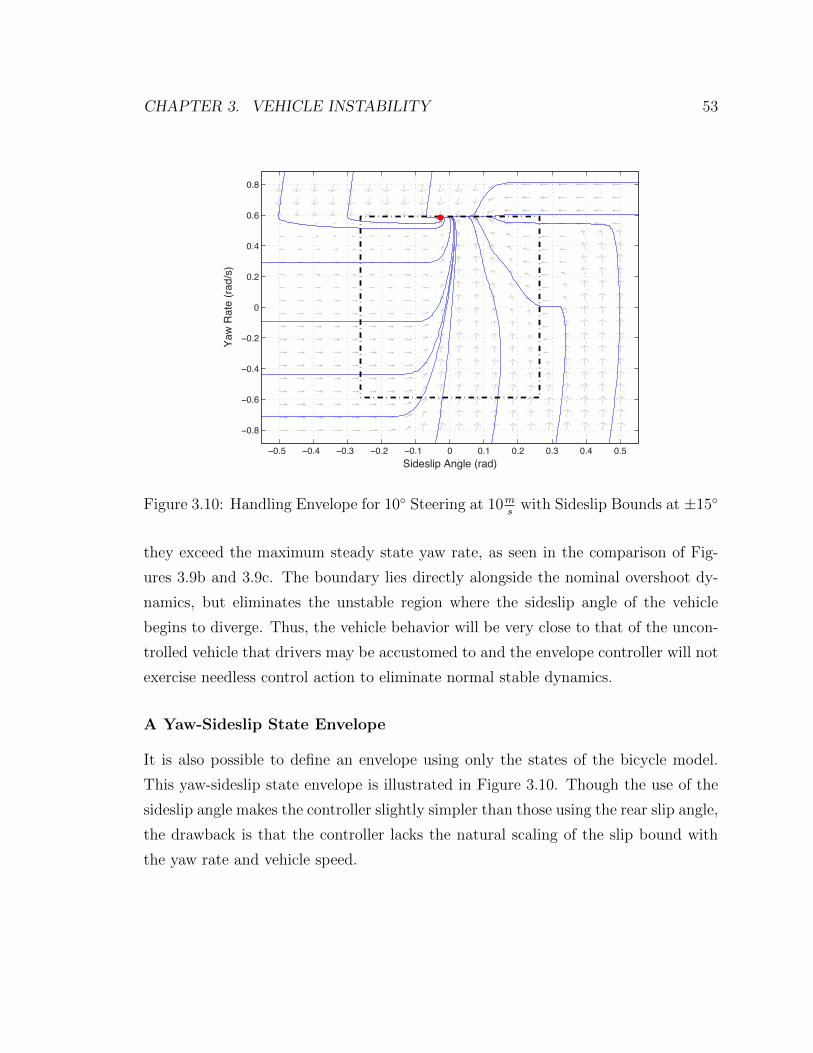
CHAPTER 3. VEHICLE INSTABILITY 53
5 4 3 2 1 1 2 3 4 5
8
6
4
2
2
4
6
8
Sideslip Angle (rad)
Yaw
Rat
e (ra
d/s)
Figure 3.10: Handling Envelope for 10◦ Steering at 10ms with Sideslip Bounds at ±15◦
they exceed the maximum steady state yaw rate, as seen in the comparison of Fig-
ures 3.9b and 3.9c. The boundary lies directly alongside the nominal overshoot dy-
namics, but eliminates the unstable region where the sideslip angle of the vehicle
begins to diverge. Thus, the vehicle behavior will be very close to that of the uncon-
trolled vehicle that drivers may be accustomed to and the envelope controller will not
exercise needless control action to eliminate normal stable dynamics.
A Yaw-Sideslip State Envelope
It is also possible to define an envelope using only the states of the bicycle model.
This yaw-sideslip state envelope is illustrated in Figure 3.10. Though the use of the
sideslip angle makes the controller slightly simpler than those using the rear slip angle,
the drawback is that the controller lacks the natural scaling of the slip bound with
the yaw rate and vehicle speed.

CHAPTER 3. VEHICLE INSTABILITY 54
An Envelope Defined by Tire Grip
One final choice of envelope is one where all of the boundaries are defined by the
angles of peak tire force. In this case, the angles at which the front and rear axles
saturate are calculated from an assumed tire model and used to restrict the vehicle
motion. This envelope, utilized in [3, 4], is diamond shaped in the state space since
lines of constant front slip angle have negative slopes. The drawback to the use of
this envelope is that it couples together the actuator and the state limits. Since
the linearized front slip angle is αf = β + aUxr − δ, this could limit the amount
of countersteer allowed by the controller in cases where the steering angle must be
changed rapidly to stabilize the vehicle.
3.3 Discussion
The insight gained from examining the dynamics suggests an alternative to the ap-
proach used in production stability control systems. This approach specifies a region
of stable handling in which the driver has full authority to control the vehicle. The
boundaries of this stable handling envelope are developed naturally from information
about the tire-road friction coefficients and scale well with vehicle speed and tire grip.
With techniques for leveraging new sensing opportunites from electric power steering
(EPS), the boundaries of these unstable regions can be reliably estimated. Variants
of the boundaries can be also be used to yield different handling characteristics at
the maximum extents of the envelope to satisfy the preferences of different drivers.
The results of this chapter serve not only to elucidate the dynamics of vehicle
instability, but also to form a basis for designers of future stability control systems to
synthesize controllers and make guarantees about vehicle performance. This frame-
work also opens up many other possibilities for vehicle control, including the use
of new or combined actuation to stabilize the vehicle, consideration of rollover or
environmental factors in determining the proper driver assistance, and the ability
to combine stability control with higher level controllers for more advanced vehicle
control tasks.

Chapter 4
Envelope Control
The previous chapter was devoted to the development of a stable handling enve-
lope that prevents the vehicle from entering undesirable handling regions. However,
the analysis was restricted to establishing the feasibility of stabilizing inputs on the
boundaries of the envelope and did not discuss a control technique for generating
these inputs. This chapter presents a model predictive envelope controller capable
of enforcing the boundaries of the safe handling envelopes and providing progressive
and smooth assistance to a human driver.
4.1 Control Strategy
In enforcing the boundaries of the envelope, the controller presented in this chapter
must satisfy two objectives. The first is that the controller must respond appropriately
in the event that a driver input would cause the vehicle to leave the envelope or that a
disturbance pushes the states outside the envelope. The second is that the controller
should track the driver’s intended vehicle behavior inside the envelope and behave in
a predictable manner when at or beyond the envelope boundaries.
Since a model predictive controller operates by solving an optimization problem to
determine a set of inputs that satisfies an objective and any constraints over a speci-
fied control time horizon at each control time step, model predictive control (MPC)
provides a straightforward method of implementing an envelope control strategy. In
55

CHAPTER 4. ENVELOPE CONTROL 56
the MPC framework, tracking the driver’s desired trajectory becomes the objective
while the envelope boundaries and actuator limits are the constraints. Furthermore,
after finding the optimal input sequence, the first input in the sequence is applied
to the system and the process is started again. In this manner, the optimization
routine needs only to find an open-loop optimal set of inputs, but the resampling and
recomputation at each time step provides a feedback loop to take into account devia-
tions from the optimal trajectory from disturbances or model error, for example. The
following subsections describe how an envelope control scheme can be implemented
in a model predictive control formulation.
4.1.1 MPC with the Affine Force-Input Model
While there are clear advantages for using model predictive control to implement
the envelope controller, there are some significant challenges in this process. Most
significant of these is the choice of model with which to inform the controller. At the
limits of handling, where the envelope controller must be active to assist the driver,
a linear model provides a poor representation of the vehicle dynamics. However,
the nonlinear brush tire models presented in Chapter 2 are both computationally
expensive and non-convex. As a result, the optimization routine used to determine the
output of the model predictive controller may run too slowly for real time operation
in a vehicle and worse yet, may produce emergent behaviors.
Convex optimization provides a solution to both of these problems. Certain classes
of optimization problems, when phrased correctly, have a single unique solution and
can be solved with computationally efficient methods [10, 44, 45, 46]. Therefore, the
definition of a convex model of the nonlinear vehicle dynamics at the handling limits
is desirable for the implementation of the model predictive envelope controller.
The rationale for using the AFI model to implement the model predictive con-
troller can be explained by examining the equations of motion for the single-track
model, given here again as Eq. 4.1. It is obvious by inspection that the equations are

CHAPTER 4. ENVELOPE CONTROL 57
linear in the front and rear lateral forces, highlighted in bold font.
β =Fyf + Fyr
mUx− r, r =
aFyf − bFyr
Izz(4.1)
The controller design presented in this chapter assumes a vehicle with rear wheel
drive and front steering, where the controller has the authority to augment the driver’s
steering command up to the limits of the actuators. In this configuration, the drive
torques and steering are located on separate axles and so the tires on the front axle
generate only lateral forces. Therefore, a manipulation of the steering can be seen
simply as a state-dependent front lateral force command. Taking this abstraction
a bit farther, the front lateral force can be viewed by the optimization solver as the
input to the system rather than the front steering angle. Thus, by changing variables,
the non-convex relationship between front lateral force and steering angle is extracted
outside the optimization solver as seen in Figure 4.1, maintaining the ability to rapidly
solve the problem while preserving the characteristics of the desired tire model.
Unfortunately, this technique does not work on the rear axle of the vehicle due to
the lack of actuation. The rear lateral tire force is a function of the vehicle states and
the longitudinal slip. Worse, this function is non-convex and is needed to accurately
calculate the predicted model states in the optimization routine. As a result, the
rear tire linearization in Eq. 2.18 is used. With the pre-solve and post-solve steps
illustrated in Figure 4.1, the resulting optimization problem is convex and thus can
Figure 4.1: MPC Block Diagram

CHAPTER 4. ENVELOPE CONTROL 58
be solved robustly and rapidly through the use of well-known convex optimization
techniques [10].
4.1.2 Envelope Boundaries
Sideslip Angle (deg)
Yaw
Rat
e (d
eg/s
)Yaw Rate Bound
Rea
r Slip
Ang
le B
ound
Figure 4.2: MPC Envelope Controller Boundaries
The envelope for the controller is a parallelogram in state space, as introduced in
the previous chapter and seen in Figure 4.2. The envelope boundaries are computed
using an approximation of the tire-road friction coefficient, which is assumed to be
estimated in real-time. It is not expected that an exact value of the friction coefficient
will be known, particularly since it is likely to be varying frequently with the changing
road surface, as seen in experimental results.
Using the friction information, the first envelope constraint is computed from the
steady-state yaw rate associated with the estimated maximum tire forces. To close the
envelope in the state plane, a second set of constraints that limit the sideslip angle are
needed. However, a simple limit on the sideslip angle has significant drawbacks when
considering the sideslip angle dependence on speed and vehicle parameterization. A
better choice for the boundary is the slip angle of the rear tire, which scales naturally
with speed and also includes the effect of yaw rate, limiting the sideslip angle at high
yaw rates. Given estimates of the vehicle cornering stiffness and tire-road friction

CHAPTER 4. ENVELOPE CONTROL 59
coefficients, Eq. 2.4c specifies the angle associated with the maximum tire force gen-
eration. Using this angle to set the maximum rear slip angle yields a conservative
envelope in which the vehicle maintains rear tire grip. However, highly skilled drivers
can maintain vehicle stability while the rear tires attain large slip angles. The same
is true of the envelope controller, and this performance can be achieved by choosing
the rear slip angle boundary to be a few degrees past the peak. In practical testing,
experienced drivers preferred the wider rear slip angle boundaries and enjoyed being
able to stably slide the vehicle with the assistance of the controller.
4.1.3 Tracking Driver Intent
Stabilizing the vehicle is an important function of an envelope controller, but to assist
the driver in guiding the vehicle along a safe trajectory, the envelope controller also
utilizes a tracking objective. There are a limited number of sensors available in pro-
duction vehicles that yield information about the driver’s intended vehicle behavior.
Thus, the control design assumes that the driver’s intended yaw rate and sideslip can
be inferred by holding the steering angle and vehicle speed constant and propagating
a linear bicycle model over a 150ms control horizon to determine the target states to
use for tracking. Away from the envelope boundaries, the linear model matches the
vehicle behavior and renders the controller silent, providing an alternative to the use
of logic to switch the controller on and off.

CHAPTER 4. ENVELOPE CONTROL 60
4.1.4 Controller Implementation
When described as a control problem for MPC, the output of the controller at each
time step is the solution to the optimization problem described here:
minimizeN�
k=1
����xkopt − xk
des
����2Wx
+N−1�
k=1
����F kyf
����2Wu
+ ηN�
k=1
����skopt����
1(4.2a)
subject to x1opt = Adxinit +BdFyfinit (4.2b)
xk+1opt = Adx
kopt +BdF
kyf + dd, (4.2c)
k = 1, . . . , N − 1
Fyfmin ≤ F kyr ≤ Fyfmax (4.2d)
k = 1, . . . , N − 1��F k
yf − F k+1yf
�� ≤ Fyfslew (4.2e)
k = 1, . . . , N − 2
Clim
��xk�� ≤ xlim + skopt (4.2f)
k = 1, . . . , N
skopt ≥ 0, k = 1, . . . , N (4.2g)
Each term in this optimization statement has physical meaning in terms of the
functionality of the envelope control system. The first term in the objective function
(Eq. 4.2a) represents the tracking objective. Thus, error between the solution tra-
jectory and the desired linear behavior is penalized through a weighted norm. This
ensures that the optimal control input tracks the driver’s desired behavior. The sec-
ond term in the input is a weighted norm on the inputs. For the controller described
here, the only input to the system is Fyf , but by defining the function as a weighted
norm on the inputs, the problem may be extended to additional actuators. The final
term in the objective function is a penalty on the slack variables that are added to the
problem to ensure that the constraints do not cause the problem to become infeasible.
The dynamic constraints (Eqs. 4.2b-4.2c) describe the dynamics that the solution
trajectory must obey. These dynamics are obtained by discretizing the continuous

CHAPTER 4. ENVELOPE CONTROL 61
Table 4.1: Description of Envelope Controller Parameters
Parameter Description
Ad Discrete State Propagation Matrix
Bd Input Effect Matrix
dd Affine Offset from Linearization
Wx State Tracking Weight Matrix
Wu Input Penalty Matrix
xdes Open Loop Trajectory from Driver Input
xinit Vehicle State at Start of Optimization
Fyfinit Front Force Input at Start of Optimization
Fyfmin Minimum Available Front Force Input
Fyfmax Maximum Available Front Force Input
Fyfslew Maximum Front Force Slew Rate
Clim Output Constraint Matrix
xlim State and Input Limits
η Stiffness of Slack Variables
AFI system given in Eq. 2.21. A Tustin discretization method is used since it offers a
closed-form solution that can easily be implemented in real time. The third constraint
(Eq. 4.2d) restricts the MPC solver to a range of inputs that are achievable given the
estimated friction coefficients and normal load on the front axle. Similarly, Eq. 4.2e
restricts the maximum change in the lateral force so that the actuator slew rate limits
are respected. Finally, Eq. 4.2f implements the constraints that define the boundaries
of the envelope. Since yaw rate is one of the system states and rear slip angle is a
linear combination of yaw rate and sideslip angle, the limit calculation matrix, Clim,
and limit vector, xlim, are:
Clim =
0 1
1 − bUx
, xlim =
rlim
αrlim
(4.3)

CHAPTER 4. ENVELOPE CONTROL 62
Predictive Time Horizon and Update Rate
The time step and horizon for the MPC problem are 10ms and 15 steps, respectively,
yielding a 150ms predictive time horizon. This horizon is well-scaled to the vehicle
control problem for two reasons. The first is that the dynamics of vehicle are fast
enough that most of the response of the vehicle to a sudden input or disturbance
can be observed in 150ms. Therefore, the controller can predict the dynamics far
enough in advance to prevent hazardous responses to these sudden events. However,
the preview horizon cannot be extended arbitrarily since error in the prediction grows
as the model is propagated forward in time. The AFI model, as presented in Sec-
tion 2.2.3, uses a single linearization of the rear tire. Because of this linearization,
the model is most accurate at the beginning of the horizon and less accurate later on
when the states move farther away from the initial conditions. Likewise, the driver
input and vehicle speed are assumed to be constant over the time horizon. Since the
longitudinal dynamics typically have bandwidth less than 1-2Hz and the responses
of skilled drivers are usually less than 3Hz, the assumption that these parameters
remain constant over the 150ms time horizon is reasonable. Furthermore, the 100Hz
update rate chosen to implement the controller means that any changes to the states,
speed, and driver input are taken into account within 10ms, leading to very good
handling of these slowly varying parameters.
4.1.5 Real Time MPC Implementation
The optimization problem that results from the envelope controller is convex, as seen
by inspection of the terms, and thus a specific set of embedded convex optimization
tools can be brought to bear on the problem. Using software such as described
in [45] and [46], custom C-code is generated which can solve the model predictive
envelope control problem with a 15-step horizon in under 2ms on a single core of an
Intel Core2 Duo processor. Despite fast solution techniques, this solve step requires
non-trivial computation time, so delay compensation is also added to the controller
as described in [17]. This is expressed in the problem formulation by Eq. 4.2b, where
the states after one time step are dictated solely by the initial conditions. By doing

CHAPTER 4. ENVELOPE CONTROL 63
this, the MPC problem is solved not for the time step at initiation of the solver, but
rather a solution is computed for the following time step when the inputs are applied.
4.2 Results and Discussion
4.2.1 Experiment: Limit Slalom Maneuver
The first set of results with the model predictive envelope controller are shown in
Figure 4.3. This test was designed to excite the vehicle dynamics with steering input
at roughly constant speed such that an uncontrolled vehicle would have left the en-
velope. To ensure consistent, clean excitation of the vehicle steering, the sinusoidal
driver steering input was generated using the vehicle computer. The envelope control
parameters are shown in Table 4.2, while the results are illustrated in Figure 4.3,
where Figure 4.3a shows the vehicle states throughout the maneuver. The surface
friction coefficient was estimated to be approximately 0.55-0.6, and so it is clear that
the vehicle is very close to the maximum lateral acceleration on each phase of the
sinusoidal maneuver.
Figure 4.3b shows the limited quantities along with the dynamically calculated
envelope boundaries. Because the boundaries are dependent upon vehicle speed, fric-
tion coefficients, and rear-wheel torque, all of which are held nearly constant, little
variation in the limits occurs through the maneuver. Examining the limited quan-
tities, it is clear that aside from a slight overshoot of the yaw rate, the controlled
vehicle remains within the envelope boundaries. However, the advantage of the enve-
lope controller goes beyond preventing major excursions of the vehicle states outside
of the envelope. Using the AFI model to predict the vehicle behavior, the controller
is capable of holding the vehicle very close to the boundaries. Assuming that the
boundaries are set at the maximum capabilities of the vehicle, the controller is capa-
ble of assisting the driver while utilizing all of the vehicle’s cornering capability while
maintaining stability.
Figure 4.3c shows the sinusoidal driver steering command as well as the total
command that is applied to the front wheels after the controller steering addition. In

CHAPTER 4. ENVELOPE CONTROL 64
25 26 27 28 29 30 31 32 33 34 35−1
−0.5
0
0.5
1
Time (s)
Stat
es (g
,rad/
s,ra
d
Lateral Accel.Yaw RateSideslip Angle
(a) Lateral Acceleration, Yaw Rate, Sideslip Angle
25 26 27 28 29 30 31 32 33 34 35−1
−0.5
0
0.5
Time (s)
Lim
its (r
ad,ra
d/s)
Yaw RateRear Slip AngleLimits
(b) Yaw Rate and Rear Slip Angle with Limits
25 26 27 28 29 30 31 32 33 34 35−20
−10
0
10
20
Time (s)
Stee
ring
Angl
e (d
eg)
Driver CommandTotal Command
(c) Driver and Total Steering Angles
25 26 27 28 29 30 31 32 33 34 35
9.910
10.110.2
Time (s)
Spee
d (m
/s)
(d) Vehicle Speed
25 26 27 28 29 30 31 32 33 34 35
−0.20
0.2
Time (s)
Torq
ue (k
Nm
)
(e) Rear Wheel Drive Torque
Figure 4.3: Experimental Results from Slalom Maneuver

CHAPTER 4. ENVELOPE CONTROL 65
this case, the driver command would cause the vehicle to exceed the boundaries of
the envelope and so the controller countersteers to compensate. An important note
here is that there is no delay in resuming the driver command once the driver steering
angle is attainable within the envelope. Therefore, there is no lag in the steering if
the driver chooses to reverse the direction of the vehicle.
4.2.2 Simulation: Slalom with Friction Variation
One other feature in the data sets seen particularly in the yaw rate and steering sig-
nals of Figure 4.3 is an oscillation around the limit. Because the gravel is unevenly
distributed on the test surface, this oscillation reflects the controller response to dis-
turbances. This can be confirmed with a simulation run where the grip properties of
each wheel are chosen from a random distribution.
Table 4.2: Envelope Controller Parameters with AFI Model
Parameter Symbol Value
MPC horizon N 15
MPC time step ∆T 0.01s
Sideslip tracking weight Wxβ5 1rad
Yaw rate tracking weight Wxr 50 srad
Input penalty weight WFyf1× 10−5 1
N
Slack variable penalty η 5× 10⁴
Input limit Fyfmax ††
Input slew rate limit Fyfslew ††
Yaw rate limit rlim ††
Rear slip limit αrlim ††
Static friction coefficient µ 0.6
Sliding friction coefficient µs 0.55
†† : Parameter is computed in real-time before optimization step.

CHAPTER 4. ENVELOPE CONTROL 66
0 1 2 3 4 5 6 7 8 9 10−0.6
−0.4
−0.2
0
0.2
0.4
(a)
Stat
es (g
,rad/
s,ra
d)
Time History Plots (time in seconds)
Lateral Accel.Yaw RateSideslip Angle
(a) Lateral Acceleration, Yaw Rate, Sideslip Angle
0 1 2 3 4 5 6 7 8 9 10
−0.4
−0.2
0
0.2
0.4
0.6
(b)
Lim
its (r
ad/s
,rad)
Yaw RateRear Slip AngleYaw Rate LimitRear Slip Limit
(b) Yaw Rate and Rear Slip Angle with Limits
0 1 2 3 4 5 6 7 8 9 10−20
−10
0
10
20
(c)
Stee
r Ang
le (d
eg)
DriverTotal
(c) Driver and Total Steering Angles
0 1 2 3 4 5 6 7 8 9 109
10
11
(d)
Spee
d (m
/s)
(d) Vehicle Speed
0 1 2 3 4 5 6 7 8 9 100
20406080
(e)
Torq
ue (N
m)
(e) Rear Wheel Drive Torque
Figure 4.4: Simulated Results from Slalom Maneuver

CHAPTER 4. ENVELOPE CONTROL 67
The conditions for the simulation were set as closely as possible to match those
of the experimental slalom shown in Figure 4.3, including identical controller pa-
rameters. The friction coefficients were varied independently for each wheel every
0.04s to represent the effect of unevenly distributed gravel. At the vehicle speed of
10 m/s, this equates to a 40cm length scale for the friction variation. The distri-
bution was assumed to be uniformly random, within the ranges µ = 0.6 ± 0.4 and
µs = 0.55±0.4. Since the friction coefficient µ always appears in the lateral tire force
expression given in Eq. 2.1 as a product with normal force, this variation can also
represent the changing normal load on a wheel.
Once the random friction conditions were incorporated into the simulation frame-
work, oscillations of approximately the same magnitude and frequency as in the ex-
periments were observed. This is particuarly apparent when looking at the first two
cycles of slalom in Figs. 4.3cc and 4.4c, where the total steering command is plotted.
Similar effects are also seen in Figs. 4.3b and 4.4b, where the yaw rate and rear slip
angles show this same oscillatory behavior.
4.2.3 Experiment: Limit Cornering with Rear Drive Torques
The previous two sets of results demonstrate the vehicle behavior when primarily
excited with steering input. However, rear-wheel drive vehicles on low-friction sur-
faces exhibit significant degradation in stability when large drive torques are applied.
Figure 4.5 shows the vehicle behavior while applying drive and braking torques to the
rear axle while cornering. This maneuver is intended to develop oversteer by reduc-
ing the available lateral force on the rear axle. A sequence of drive-brake-drive-brake
torques at the actuator limits is used to provide multiple instances of excitation to
test the controller. Figure 4.5 shows the results from the maneuver and the controller
parameters are again those given in Table 4.2.
As with the previous figures, Figure 4.5a is a plot of the yaw rate, sideslip angle,
and lateral acceleration. Figure 4.5b illustrates the yaw rate and rear slip angles
along with their limits. In this case the limits are a bit more interesting, as the rear
wheel torque and speed profiles (seen in Figs. 4.5d and 4.5e) significantly affect the

CHAPTER 4. ENVELOPE CONTROL 68
18 19 20 21 22 23 24 25 26−0.5
0
0.5
1
Time (s)
Stat
es (g
,rad/
s,ra
d
Lateral Accel.Yaw RateSideslip Angle
(a) Lateral Acceleration, Yaw Rate, Sideslip Angle
18 19 20 21 22 23 24 25 26−1
−0.5
0
0.5
Time (s)
Lim
its (r
ad,ra
d/s)
Yaw RateRear Slip AngleLimits
(b) Yaw Rate and Rear Slip Angle with Limits
18 19 20 21 22 23 24 25 26−5
0
5
Time (s)
Stee
ring
Angl
e (d
eg)
Driver CommandTotal Command
(c) Driver and Total Steering Angles
18 19 20 21 22 23 24 25 2610
12
14
Time (s)
Spee
d (m
/s)
(d) Vehicle Speed
18 19 20 21 22 23 24 25 26
−0.50
0.51
1.5
Time (s)
Torq
ue (k
Nm
)
(e) Rear Wheel Drive Torque
Figure 4.5: Experimental Results from Cornering with Torque Disturbances

CHAPTER 4. ENVELOPE CONTROL 69
Table 4.3: Envelope Controller Parameters with Linear Model
Parameter Symbol Value
MPC horizon N 15
MPC time step ∆T 0.01s
Sideslip tracking weight Wxβ5 1rad
Yaw rate tracking weight Wxr 50 srad
Input penalty weight Wδ 1 1rad
Slack variable penalty η 5× 10⁴
Input limit δlim ±22◦
Input slew rate limit δslew ±140◦/s
Front slip limit αflim ±8◦
Rear slip limit αrlim ±8◦
†† : Parameter is computed in real-time before optimization step.
limits. For example, at approximately 22.5s the accelerator is depressed to command
maximum torque. The yaw rate and rear slip angle limits are instantly decreased
since the MPC controller calculates that the maximum achievable values are lowered.
However, the vehicle states cannot respond instantaneously, and so for several time
steps the states are outside the new, smaller envelope. The controller therefore coun-
tersteers hard to bring the states inside the envelope and then returns the vehicle
again to the boundary, giving the driver the maximum possible cornering capability.

CHAPTER 4. ENVELOPE CONTROL 70
4.2.4 Experiment: Control Performance with Linear Model
The representation of rear tire saturation in the AFI model (Eq. 2.18) is critical in
obtaining the performance of the envelope controller seen in Figure 4.5. Without
the prediction of decreased rear lateral force, the controller would be incapable of
responding accurately to the rapid growth in rear slip angle. To illustrate the necessity
of this information, a set of experiments was performed with a purely linear tire
model used to predict the forces that would be developed on each axle. Figure 4.6
demonstrates a lift-off oversteer on a mixed dirt and gravel surface. For this test, the
model underlying the controller utilized a static linearization about zero slip angle at
the rear axle and assumed a purely linear mapping between front steering angle and
front lateral tire force. A front slip angle limit also replaced the yaw rate constraint.
The parameters of this model, seen in Table 4.3, were chosen to allow the tires to get
to full saturation.
Figure 4.6a shows the vehicle states throughout the maneuver. Note here that the
vehicle has already entered a corner at 56s when the timeline of the plot begins. The
driver continues to increase the steering angle (seen in Figure 4.6c) until reaching a
limit understeering case where the controller countersteers to keep the front slip an-
gle near the envelope boundary. There is a small steady-state error during the initial
cornering phase as a result of the tire model overstating the effect of steering input
near tire saturation. Usage of the AFI model avoids this by including the saturation
dynamics in the steering angle calculation. When the driver applies drive torque to
the rear axle, the rear slip angle increases dramatically. The controller countersteers,
but the tire model mismatch results in a poor prediction of the dynamics in this highly
nonlinear region and thus a violation of the envelope boundary occurs. Because the
linear model has no representation of this tire saturation, the controller underesti-
mates the steering input needed to stabilize the vehicle. The countersteer maneuver
does eventually return the vehicle to the envelope, and the controller is successful in
stabilizing the vehicle in the lift-off oversteer maneuver.

CHAPTER 4. ENVELOPE CONTROL 71
35 40 45 50 55 60 65−1.5
−1
−0.5
0
0.5
1
Time (s)
Stat
es (g
,rad/
s,ra
d
Lateral Accel.Yaw RateSideslip Angle
(a) Lateral Acceleration, Yaw Rate, Sideslip Angle
35 40 45 50 55 60 65−0.5
0
0.5
Time (s)
Lim
its (r
ad,ra
d)
Front Slip AngleRear Slip AngleLimits
(b) Yaw Rate and Rear Slip Angle with Limits
35 40 45 50 55 60 65−20
−10
0
10
20
30
Time (s)
Stee
ring
Angl
e (d
eg)
Driver CommandTotal Command
(c) Driver and Total Steering Angles
35 40 45 50 55 60 65
56789
Time (s)
Spee
d (m
/s)
(d) Vehicle Speed
35 40 45 50 55 60 65−1
012
Time (s)
Torq
ue (k
Nm
)
(e) Rear Wheel Drive Torque
Figure 4.6: Experimental Results from Lift-off Oversteer Maneuver

CHAPTER 4. ENVELOPE CONTROL 72
4.2.5 Experiment: Control with Wide Slip Boundaries
In Chapter 3, a series of alternative envelopes were presented, including an envelope
with extended rear slip angle boundaries intended to allow a driver to saturate the rear
tires and allow the car to slide without losing control. Figure 4.7 demonstrates the
performance of the vehicle while under envelope control with this enlarged envelope.
The rear slip angle boundaries are set to a static value of 20◦ for the maneuver and
the driver performs a lift-off oversteer followed by a double lane change. In the lift-off
oversteer, the driver lifts off the accelerator pedal while cornering as seen by the plot
of the states in Figure 4.7a and the torque input in Figure 4.7e, producing braking
torque and resulting in a significant rear tire saturation and the rear axle beginning
to slide. However, once the rear slip angle gets near the boundary, the controller
countersteers as seen in Figure 4.7c and holds the rear slip angle approximately at
the boundary (Figure 4.7b) until the driver begins to reduce the braking torque and
steer out of the turn. Later in the data set, the driver performs a double lane change
at approximately 12ms . Though the double lane change excites both the yaw and slip
dynamics of the vehicle, the rear slip angle remains well away from the limit and only
the yaw rate constraint is enforced.

CHAPTER 4. ENVELOPE CONTROL 73
55 60 65 70 75 80 85−1
−0.5
0
0.5
1
Time (s)
Stat
es (g
,rad/
s,ra
d
Lateral Accel.Yaw RateSideslip Angle
(a) Lateral Acceleration, Yaw Rate, Sideslip Angle
55 60 65 70 75 80 85−1
−0.5
0
0.5
Time (s)
Lim
its (r
ad,ra
d/s)
Yaw RateRear Slip AngleLimits
(b) Yaw Rate and Rear Slip Angle with Limits
55 60 65 70 75 80 85
−10
0
10
20
Time (s)
Stee
ring
Angl
e (d
eg)
Driver CommandTotal Command
(c) Driver and Total Steering Angles
55 60 65 70 75 80 85468
1012
Time (s)
Spee
d (m
/s)
(d) Vehicle Speed
55 60 65 70 75 80 85
−1
0
1
Time (s)
Torq
ue (k
Nm
)
(e) Rear Wheel Drive Torque
Figure 4.7: Experimental Results with Wide Rear Slip Angle Boundaries

CHAPTER 4. ENVELOPE CONTROL 74
4.3 Guaranteeing Controller Action
The following subsections examine the action of the vehicle under envelope control
to demonstrate that the controller is capable of keeping the vehicle inside the safe
handling in the absence of disturbances and acts appropriately to attract the vehicle
to the envelope in cases where disturbances or sudden reductions in envelope size
cause the states to lie outside the boundaries of the envelope. These analyses are
based on the assumption that the vehicle behavior is accurately described by a linear
bicycle model with nonlinear brush tires as described in Chapter 2. In cases where the
action of the controller using the AFI model is considered, the it is assumed that the
AFI model is linearized at every point considered and thus yields the same response
as the nonlinear model at each point. Error between these models and the behavior
of the real vehicle is known to be minor and in many cases will be less than the error
incurred through the utilization of an estimate of the real friction coefficient.
4.3.1 Envelope Invariance Proof
A proof that the model predictive envelope controller stabilizes the vehicle, regardless
of the driver input, is presented in this section. Since the controller is not easily
expressed in a closed form, the proof is presented by examining the range of stabilizing
inputs and showing that the optimization will produce these inputs as the MPC input
to the vehicle.
The proof presented here leaves out the slew rate limits for clarity. The test vehicle
used in experiments with the controllers described in this paper has an extremely fast
steering system [40] for which the slew rate constraints appear to be unrestrictive.
Theory of Exact Penalty Functions
It is common for a model predictive controller to contain, at its core, an optimization
problem with both state and input constraints. As mentioned in the previous section,
if both of these constraints are hard constraints, then the problem may be infeasible at
some points. This can occur either due to the constraints being incompatible at some
point in the state space or due to disturbances causing the states to deviate outside
CHAPTER 4. ENVELOPE CONTROL 75
the boundaries of the state constraints. In either case, the controller is incapable
of determining a control action, so the constraints are softened in order to ensure
problem feasibility. The drawback to softening the constraints is that the guarantee
of controller action in the case that the original hard-bounded problem was feasible is
lost. Fortunately, the theory of exact penalty functions provides a means to recover
this guarantee.
In a paper by Han and Mangasarian [25], the authors describe the use of exact
penalty functions with a hard-constrained optimization problem of the form:
minimize f(x) (4.4a)
subject to g(x) ≤ 0 (4.4b)
h(x) = 0 (4.4c)
where f, g, and h are functions from Rn into R, Rm, and Rk respectively. A point
x in Rn satisfying the constraints is considered to be a feasible point. This problem
can be re-expressed as an optimization problem with no constraints, but with a cost
associated with any non-feasible point.
minimize f(x) + αQ (||g(x)+, h(x)||) (4.5)
where α is a nonnegative real number, g(x)+ is a penalty on any positive value of
g(x), and Q is a function that satisifies
Q(0) = 0 (4.6a)
Q(ζ) > 0 for ζ > 0 (4.6b)
If Q(ζ) = ζ and the one-norm is used, then this problem becomes
minimize f(x) + α
�m�
j=1
gj(x)+ +k�
j=1
|hj(x)|�
(4.7)
and is of exactly the same form used for the envelope control problem. The results

CHAPTER 4. ENVELOPE CONTROL 76
presented by Han and Mangasarian demonstrate that given this problem, there is a
condition on the penalty weight that is defined by the dual norm of the Lagrange
dual optimal inequality and equality multipliers λ and ν, for the original problem. If
α > α with
α = ||λ, ν||∞ (4.8)
then a solution to the soft-bounded problem will also be a solution to the hard-
bounded problem, provided that the hard-bounded problem is feasible.
The hard-constrained envelope control problem can be expressed as a standard-
form quadratic program with linear constraints, which is:
minimize xTPx+ qTx+ r (4.9a)
subject to A1x− b1 ≥ 0 (4.9b)
A2x− b2 = 0. (4.9c)
Therefore, the Lagrange dual problem can be expressed as:
maximize r − λT b1 − νT b2 (4.10a)
subject to q + A1λ+ A2ν (4.10b)
λ ≥ 0. (4.10c)
For each combination of A1, A2, b1, b2, q, and r, there is an associated condition on the
penalty weight defined, as before, by the dual norm of the optimal multiplying factors,
λ∗ and ν∗. Since the desired soft-constrained problem uses the 1-norm to penalize the
slack variables, the dual norm is the infinity-norm. Therefore, the condition needed
for the envelope control problem slack weight is
η > supA1,A2,b1,b2,q,r
||λ∗, ν∗||∞ (4.11)
With respect to the envelope control problem, this establishes that if the slack
weight η is chosen to be sufficiently large and an input exists that prevents the vehicle
from leaving the envelope, this input will be the solution to the optimization problem.

CHAPTER 4. ENVELOPE CONTROL 77
Feasibility of the Envelope
In order to determine that a feasible input is present for all points on the boundary,
the envelope is examined in each quadrant, as illustrated in Figure 4.8. In Quadrant
I, the yaw rate and sideslip angle are both positive. Quadrant II contains states with
positive yaw rates and negative sideslip angles. Quadrant III has negative yaw rates
and sideslip angles and is symmetric to Quadrant I. Finally, Quadrant IV contains
negative yaw rates and positive sideslip angles and is symmetric to Quadrant II.
Beginning with Quadrant II, in which open-loop equilibria for left turns lie, if
they exist, the conditions for remaining in the envelope when on the boundary can
be written as
r ≤ 0, αr ≥ 0. (4.12)
If, at every point on the boundary, these conditions can be satisfied, then the model
predictive controller can find an input that will, at the first time step, keep the states
from exiting the boundary. At subsequent steps in the time horizon, the predicted
states may move away from the linearization point. As such, there may be error in
the prediction, but exits from the envelope will still be prevented since only the first
time step will elapse before the solution is recomputed.
The conditions on the states must be expressed in terms of the input, Fyf to ensure
that they are feasible at every point on the boundary of the envelope. Beginning with
the yaw rate, a bound on the input, Fyf is computed.
r =aFyf − bFyr
Izz≤ 0 =⇒ Fyf ≤ b
aFyr (4.13)
Given sufficient steering range on the vehicle, this condition is easily achievable since
Fyr is positive in Quadrant II and thus any negative Fyf is acceptable.
The rear slip angle derivative is comprised of a linear combination of the yaw rate
and sideslip angle derivatives, and is thus more complicated than the yaw rate deriva-
tive. However, this can be handled in the same manner as the yaw rate derivative.

CHAPTER 4. ENVELOPE CONTROL 78
Quadrant I
r > 0, β > 0
α > 0, Fy < 0
Quadrant II
r > 0, β < 0
α < 0, Fy > 0
Quadrant III
r < 0, β < 0
α < 0, Fy > 0
Quadrant IV
r < 0, β > 0
α > 0, Fy < 0
r
β
Figure 4.8: Four quadrants of the state space used for the proof
Beginning with the expression for the rear slip angle derivative,
αr = β − b
Uxr ≥ 0 (4.14a)
Fyf + Fyr
mUx− r − b
Uxr ≥ 0. (4.14b)
Since the yaw rate condition must simultaneously hold, r is known to be negative,
and it is clear that with r ≤ 0, and m, Ux, Izz, and Fyr all positive quantities, a
somewhat conservative condition can be written as:
Fyf + Fyr
mUx≥ r (4.15)
On the boundary, αr = αrmax , the rear tire is already fully saturated, yielding Fyr =
Fyrmax. Considering the case where the input is chosen to yield the least restriction
on the yaw rate, Fyf = baFyrmax
, this reduces to
Fyrmax
�1 + b
a
�
mUx≥ r (4.16)

CHAPTER 4. ENVELOPE CONTROL 79
which is the yaw rate boundary of the envelope. Therefore, when inside the bounds,
a feasible input may always be found which will prevent the vehicle from leaving the
envelope. The same result holds for Quadrant IV by symmetry.
Quadrants I and III are considered pathological cases of the vehicle control scheme
since these combinations of states can only be possible in transient cases and have
not been observed in experiment. However, the dynamics of the controlled vehicle
can be illustrated in the same way as with Quadrants II and IV. In Quadrant I, the
slip angle condition changes sign, yielding the following conditions for maintaining
the vehicle in the envelope.
r ≤ 0, αr ≤ 0. (4.17)
Beginning with the yaw rate equation like Quadrant II, the same condition on the
front lateral force may be derived.
r =aFyf − bFyr
Izz≤ 0 =⇒ Fyf ≤ b
aFyr (4.18)
However, unlike Quadrant II, the rear lateral force, Fyr is negative. Therefore, at the
positive slip angle boundary, the input Fyf must be saturated at its minimum value
to meet the yaw rate condition. This yields Fyf = baFyr and r = 0, Thus, while it is
not possible to reduce the yaw rate everywhere, there is an input at every point on
the boundary that prevents the yaw rate from growing and keeps the vehicle within
the envelope.
This yaw rate condition also makes analysis at the slip angle boundary simple.
Since the best-case input on the slip angle boundary yields r = 0 with Fyf = baFyr,
these values may be substituted into the slip angle dynamics.
αr = β − b
Uxr ≤ 0 (4.19a)
Fyf + Fyr
mUx− r − b
Uxr ≤ 0 (4.19b)
Fyr
�1 + b
a
�
mUx− r ≤ 0 (4.19c)
In Quadrant I, Fyr ≤ 0 and r ≥ 0 and thus the rear slip angle is reduced when the

CHAPTER 4. ENVELOPE CONTROL 80
yaw rate condition is satisfied. Again, the same conditions hold in Quadrant III by
symmetry.
Statement of the Proof
Theorem 1. If, (1) the vehicle states are initially within the envelope, and (2) an
input exists at every point on the envelope boundary that drives the system states to
the interior of the envelope and (3) the penalty weight on the slack variables in the
optimization problem is chosen according to Eq. 4.11, the vehicle cannot leave the
envelope.
Proof. Given that the vehicle starts inside the boundaries of the envelope, it is known
from solving the appropriate linear programs that
10 ≥ η > supA1,A2,b1,b2,q,r
||λ∗, ν∗||∞ , (4.20)
The actual slack weight for the controller is set at 50,000 for good performance in
cases with disturbances that result in the vehicle outside the boundaries. Thus, since
the results demonstrate that an input exists on every point on the boundary that
keeps the states from leaving the envelope, the hard-constrained problem is feasible.
Therefore, the model predictive controller with sufficient slack weight will always
select an input that preserves the invariance of the envelope.
4.3.2 Envelope Attraction
A demonstration that the envelope controller attracts the vehicle states to the enve-
lope is possible by leveraging the optimality of the solution to the model predictive
control problem. Since the controller solution will produce a trajectory with the low-
est cost, it can be seen that inputs that attract the vehicle states to the envelope
result in a smaller cost function than inputs that allow the vehicle states to drift
away and therefore the controller will attract the vehicle to the envelope.
CHAPTER 4. ENVELOPE CONTROL 81
Optimality of the Objective Function
The result of the optimization problem will seek to minimize the following objective
function:
minimizeN�
k=1
����xkopt − xk
des
����2Wx
+N−1�
k=1
����F kyf
����2Wu
+ ηN�
k=1
����skopt����
1(4.21)
This objective function is dependent on both the input chosen and the resulting
vehicle trajectory. Each summation may be examined to determine its effect on the
output of the optimization. The first term in Eq. 4.21 minimizes deviation from
the desired trajectory. While the desired trajectory is chosen based on the vehicle
state and driver steering input, it is always restricted within the boundaries of the
envelope. Therefore, any xopt that is outside the envelope incurs cost in this term and
the optimization will seek a trajectory that draws the vehicle closer to the nearest
point on the envelope.
The second term in Eq. 4.21 is the sum of the force input required to achieve
the desired trajectories. This term is added to the objective function with a low
weight to incentivize small inputs when other criteria are satisfied. This term has the
potential to push the solution for the vehicle trajectory away from the envelope, but
since the maximum front lateral force is restricted, this term is bounded and small,
and therefore has little influence on the solution.
The third and final term in Eq. 4.21 is the penalty on the slack variables. During
normal operation inside the envelope, this term is zero. When outside the envelope,
a large value of η causes this term to become dominant. Since the term is the sum of
the linear deviations of both the sideslip and yaw rate states in the optimal trajectory,
this term heavily penalizes any solution that does not return the states toward the
envelope.
4.3.3 Feasible Trajectories
From the discussion of the terms in the objective function, the ideal trajectory for an
initial condition outside the envelope would seem to be along a line in the direction of

CHAPTER 4. ENVELOPE CONTROL 82
the nearest point on the envelope. However, the saturation dynamics of the tires may
prevent the controller from achieving this trajectory. For example, Eq. 4.16 in the
previous section demonstrated that when the rear tire is saturated and the vehicle is
within the yaw rate bounds, the sideslip angle may always be reduced. However, this
result may be reversed as well. In order to reduce the magnitude of the sideslip angle
in Quadrant II,
β =Fyf + Fyr
mUx− r > 0 (4.22)
However, if the vehicle is already outside of both the yaw rate and the slip angle
boundaries, then
r = γFyrmax
�1 + a
b
�
mUx, andFyr = −Fyrmax (4.23)
with γ ≥ 1. Therefore,
β =Fyf + Fyrmax
mUx− γ
Fyrmax
�1 + a
b
�
mUx(4.24a)
=Fyf − γ a
bFyrmax
mUx(4.24b)
Assuming the nominal weight distribution for the vehicle, the maximum front force
is statically related to the rear force, Fyf = abFyrmax . Thus,
β =Fyf − γ a
bFyrmax
mUx(4.25a)
=(1− γ) a
bFyrmax
mUx(4.25b)
β ≤ 0 (4.25c)
which shows that outside the yaw rate and slip boundaries, it is not possible to directly
increase the sideslip angle. Instead the yaw rate must first be reduced until it is below
the bound, where the sideslip angle may be increased to re-enter the envelope.
Figure 4.9 illustrates a situation where the vehicle encounters a sudden reduction
of the friction coefficient from 1.0 to 0.1. The vehicle, which was operating at the

CHAPTER 4. ENVELOPE CONTROL 83
−30 −25 −20 −15 −10 −5−0.2
0
0.2
0.4
0.6
0.8
1
Sideslip Angle (deg)
Yaw
Rat
e (ra
d/s)
Figure 4.9: Feasible Envelope Re-entry Trajectory
edge of the envelope for the high friction surface, illustrated by the red dotted line,
is suddenly well outside the envelope. Several bundles of arrows are plotted on the
figure to demonstrate the direction of possible trajectories at various yaw rates. The
arrows at the extremes represent the trajectories associated with Fyfmax and Fyfmin .
Note that above the yaw rate limit of the smaller new envelope, these arrows show
that the sideslip angle grows regardless of the chosen input. The resulting action of
the controller is to maximize the reduction in yaw rate until it is possible to increase
the sideslip angle and re-enter the new envelope for the changed friction conditions,
illustrated by the black line.
This action represents the best case recovery for a vehicle using front-wheel steer-
ing for actuation. Unfortunately, the dynamics of the vehicle dictate that the rear slip
angle will grow before recovering. In this case, the rear slip angle grew to a maximum
deviation of 10◦ from the boundary before recovering.

CHAPTER 4. ENVELOPE CONTROL 84
Tire
For
ce
Slip Angle
Saturation SlewDistance
Total Slew Distance
Figure 4.10: Slew Distance for Change of Tire Force
4.3.4 Effect of Actuator Limits
In Figure 4.9, the steering system was assumed to be able to immediately attain the
slip angle required to generate Fyfmin and reduce the yaw rate. However, to operate
near the boundary of the initial high-friction envelope, the steering system is typically
producing nearly the maximum front force and would thus have to slew the wheels
from one side to the other to countersteer and reduce the vehicle yaw rate. Worse yet,
the reduction in friction coefficent also causes a reduction in the slip angle associated
with peak lateral force. As a result, the steering system must slew through the region
of saturated maximum tire force before finally reaching a point where lateral force
begins to decrease, as seen in Figure 4.10. This extended period in which the tire
remains in saturation and produces the worst-case force drastically increases the rear
slip angle growth, as seen in Figure 4.11.
This analysis underscores the importance of utilizing fast actuators and minimiz-
ing system delays in implementing the envelope control system. In situations with
sudden disturbances or friction changes, a substantial and rapid intervention must

CHAPTER 4. ENVELOPE CONTROL 85
−35 −30 −25 −20 −15 −10 −5
−1
−0.8
−0.6
−0.4
−0.2
0
0.2
0.4
0.6
0.8
1
Sideslip Angle (deg)
Yaw
Rat
e (ra
d/s)
Figure 4.11: Envelope Re-entry with Slew Rate Limitation
be made. This also highlights the opportunities for assisting a human driver, since
many drivers will initially fail to recognize the change in the driving conditions. Fur-
thermore, once the driver has made the decision to act, there is an additional delay
before physical action can be taken. Therefore, the fast response of the envelope
control system can prevent the vehicle from spinning out and give the driver time to
regain control.
4.4 Summary
The analysis presented in this chapter shows that the model predictive envelope con-
troller augments the vehicle dynamics in precisely the desired manner so that the
driver is provided with the assistance needed to maintain stability of the vehicle. The
invariance proof presented in Section 4.3.1 demonstrates that the controller is capa-
ble of keeping the vehicle within the specified envelope boundaries when the vehicle
speed, tire-road friction coefficient, and rear wheel torques remain constant.

CHAPTER 4. ENVELOPE CONTROL 86
Unfortunately, these quantities vary in normal driving and may change drastically
in an emergency situation. In many cases, the envelope size may increase as a result in
favorable changes in these parameters. However, in critical situations, the envelope is
much more likely to decrease in size. If this reduction of the envelope occurs quickly,
such as in the case of a sudden drop in friction, it will outpace the dynamics of the
vehicle and the actuators and result in the vehicle states being outside the envelope. In
this case, the analysis of envelope attraction presented in Section 4.3.2 demonstrates
that the model predictive controller will utilize maximum actuator authority to bring
the vehicle back into the envelope. The extreme and unlikely case of a sudden drop
in the friction coefficient from 1.0 to 0.1 demonstrates that while the dynamics of
the vehicle and the actuators prevent the controller from driving the states directly
into the envelope, the controller achieves the best possible return to the envelope,
providing maximum assistance to the driver in maintaining stability.

Chapter 5
Real Time Estimation
In order for the controller described in the previous chapter to work in real world
driving conditions, the boundaries of the safe handling envelope must be continu-
ously updated to reflect changing conditions in the environment. However, because
direct measurement of the tire-road friction coefficient is impractical and GPS or
optical measurements of the vehicle sideslip angle are relatively expensive and some-
times obscured, these quantities that dictate the size of the vehicle envelope must be
estimated. This chapter describes the integration of the envelope controller with an
estimator that utilizes inexpensive and readily available steering effort and chassis
inertial measurements to produce estimates of these important quantities that are
suitable for use in the model predictive envelope controller. Despite the challenges
of estimation and control on a highly variable surface, experimental results demon-
strate that the coupled system is capable of suitably restricting the vehicle motion
and preventing undesirable vehicle behavior.
5.1 Estimation Technique
The estimation technique chosen to supply slip angles and real time friction infor-
mation to the envelope controller utilizes steering torque and steering angle measure-
ments to supplement measurements of yaw rate and lateral acceleration supplied by
standard automotive grade inertial sensors. This coupled slip angle and peak force
87

CHAPTER 5. REAL TIME ESTIMATION 88
estimator is the same structure as the one presented by Hsu and Gerdes in [31].
5.1.1 Slip Angle Estimation
The slip angle dynamics for the front axle are straightforward to derive from the
bicycle model. Assuming small angles and constant longitudinal speed, the derivative
of the front slip angle is
αf = β +a
Uxr − δ (5.1)
where β and r are defined by the basic bicycle model equations as presented in
Equation 2.15. With these relationships substituted, the front slip angle is seen to be
a function of the front and rear axle forces, the yaw rate, and the steering rate.
αf =
�1
mUx+
a2
IzV
�Fyf +
�1
mUx− ab
IzV
�Fyr − r − δ (5.2)
The yaw rate and steering rate are directly measurable, but the lateral forces must
be estimated simultaneously with the slip angle. Assuming these force estimates are
available, the resultant observer dynamics for the slip angle estimate are
�αf =
�1
mUx+
a2
IzV
��Fyf +
�1
mUx− ab
IzV
��Fyr−r− δ+K
��Fyf + �Fyr −may
�(5.3)
where ay is directly measurable and K is the observer gain. To obtain estimates of the
forces, a single coefficient version of the brush tire model described in Section 2.1.1
is used in combination with the slip angle estimate. This model describes the lateral
forces as a function of slip angle, normal load, and friction coefficient.
Fy = −Cα tanα +C2
α
3µFz|tanα| tanα− C3
α
27µFztan3 α (5.4)
The cornering stiffness, Cα, can be estimated offline. Unfortunately, the normal load
and friction coefficient vary in real time. However, these quantities appear only as a
product with each other in the denominator of the tire force model. Therefore, a new

CHAPTER 5. REAL TIME ESTIMATION 89
quantity referred to as “inverted peak force” may be defined as
If =1
µFz, (5.5)
reducing the real time task to that of estimating a single parameter. The resulting
tire model, written in terms of the inverted peak force, is
Fy = Cα tanα− C2αIf3
|tanα| tanα +C3
αIf27
tan3 α. (5.6)
Thus, with an estimate of If , the necessary sideslip angle and peak force may be
calculated and used to inform the model predictive envelope controller. Since nor-
mal load can be roughly estimated from the lateral and longitudinal acceleration
measurements and an a priori measurement of vehicle mass, Fz can also be readily
estimated. Therefore, it is straightforward to convert between If and µ and these
quantities will be used interchangeably in the description of the coupled estimation
and control structure.
5.1.2 Peak Force Estimation
To understand the inverted peak force estimation scheme, one must first understand
the mechanism by which tire forces generate torques about the steering axis. There
are three tire forces that are reacted by the suspension: the lateral force, the normal
load, and longitudinal force from drive and braking. In a typical suspension design,
the steering axis is inclined in both the lateral and longitudinal directions. The
resulting angles between the steering axis and the vertical direction are referred to as
the kingpin and caster angles, respectively, as seen in Figure 5.1. In many suspension
designs, these angles result in the intersection of the steering axis and the ground
being offset from the center of the tire contact patch. In the lateral direction, this
offset is referred to as scrub radius, while in the longitudinal direction, it is referred
to as trail.
The torque that the steering system of the vehicle must resist is produced as a
result of these offsets and the forces generated by the tire. Because the lateral force
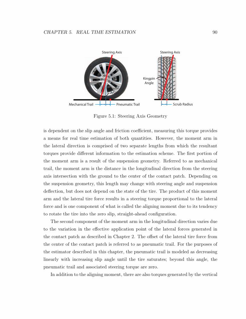
CHAPTER 5. REAL TIME ESTIMATION 90
Steering Axis Steering Axis
KingpinAngle
CasterAngle
Pneumatic Trail Scrub RadiusMechanical Trail
Figure 5.1: Steering Axis Geometry
is dependent on the slip angle and friction coefficient, measuring this torque provides
a means for real time estimation of both quantities. However, the moment arm in
the lateral direction is comprised of two separate lengths from which the resultant
torques provide different information to the estimation scheme. The first portion of
the moment arm is a result of the suspension geometry. Referred to as mechanical
trail, the moment arm is the distance in the longitudinal direction from the steering
axis intersection with the ground to the center of the contact patch. Depending on
the suspension geometry, this length may change with steering angle and suspension
deflection, but does not depend on the state of the tire. The product of this moment
arm and the lateral tire force results in a steering torque proportional to the lateral
force and is one component of what is called the aligning moment due to its tendency
to rotate the tire into the zero slip, straight-ahead configuration.
The second component of the moment arm in the longitudinal direction varies due
to the variation in the effective application point of the lateral forces generated in
the contact patch as described in Chapter 2. The offset of the lateral tire force from
the center of the contact patch is referred to as pneumatic trail. For the purposes of
the estimator described in this chapter, the pneumatic trail is modeled as decreasing
linearly with increasing slip angle until the tire saturates; beyond this angle, the
pneumatic trail and associated steering torque are zero.
In addition to the aligning moment, there are also torques generated by the vertical

CHAPTER 5. REAL TIME ESTIMATION 91
and longitudinal tire forces. Since the normal force on the tire acts roughly at the
center of the contact patch, this offset of the steering axis results in a moment arm that
causes a torque to be exerted about the steering axis. This is known as jacking torque
and varies only with changing normal load. Although this normal load changes with
the dynamic state of the vehicle, it does not provide useful information for estimating
the friction coefficient. Thus, for use in the estimator, the jacking torque is estimated
from other vehicle state measurements and removed from the total steering torque
measurement.
The drive and braking torques on the wheel also result in torque being applied
to the steering system. The component of the scrub radius that is perpendicular to
the steering axis defines the moment arm for this effect. This torque can also be
calculated and removed from the steering torque measurements used for estimation,
but for tests performed with the P1 experimental testbed, no drive or braking torques
are applied to the front axle during estimation and so no compensation is necessary.
Thus, the aligning moment needed for estimation can be found from the steering
torque measurement by subtracting the jacking torque and any dynamic effects from
the wheel and tire assembly:
Malign = Mloadcell − Fzljacking − bdampingωwheel − sgn (ωwheel)Fcoulomb (5.7)
where Mloadcell is the steering effort measured by load cells in the steering tie rods,
ljacking is the jacking moment arm calculated from the suspension geometry, and
bdamping and Fcoulomb are found through system identification of the steering and sus-
pension systems. The resulting aligning moment may be used to generate an estimate
of the pneumatic trail if the mechanical trail is known and an estimate of lateral force
is available, as seen from the following equation.
�tp = −Malign
�Fyf
+ tm (5.8)
In the case of the coupled observer structure presented here, the lateral force estimate
from the previous time step is utilized to generate the pneumatic trail value.

CHAPTER 5. REAL TIME ESTIMATION 92
0 0.05 0.1 0.15 0.20
0.1
0.2
0.3
0.4
0.5
0.6
0.7
0.8
0.9
1
Slip Angle α
|Fy/(F
z)|
Lateral Tire Force
µ = 1µ = 0.5µ = 0.2
0 0.05 0.1 0.15 0.20
0.1
0.2
0.3
0.4
0.5
0.6
0.7
0.8
0.9
1
Slip Angle α
t p/t po
Pneumatic Trail
µ = 1µ = 0.5µ = 0.2
Figure 5.2: Lateral Force and Linear Pneumatic Trail Models
The benefit of calculating pneumatic trail for estimation is clear from Figure 5.2,
which illustrates the evolution of lateral tire forces and pneumatic trails for various
friction conditions as the slip angle of the tire increases. At low slip angles, the
lateral tire force is unrelated to the friction coefficient and yields no information
for the estimator. However, the model of pneumatic trail illustrated in Figure 5.2
decreases linearly with slip angle and friction coefficient until tire saturation and thus
can be used to interpret the inertial and steering torque measurements to arrive at
an estimate of the peak force capabilities of the vehicle. This piecewise linear model
for pneumatic trail can be expressed as:
�If =
3(tp0−�tp)tp0Cα|tan �α| if �α ≤ tan−1
�3
Cαf If
�
|Mmeas|tm
otherwise(5.9)
where tp0 and Cα are estimated offline and �α is the previous front axle slip estimate.
This coupled estimation process is outlined in Figure 5.3. A proof that the coupled
structure is stable is presented in the work by Hsu and Gerdes [31].
5.1.3 Practical Considerations
Although the estimation scheme is capable of handling a wide range of driving con-
ditions, there are regimes in which the estimator does a poor job of estimating as
a result of limited excitation. To avoid the generation of poor estimates in these

CHAPTER 5. REAL TIME ESTIMATION 93
[algebraic]
[dynamic]
Figure 5.3: Coupled Sideslip and Friction Estimator Flowchart [31]
regimes, additional logic is added to the estimation structure.
The first of these logic switches is based on speed and causes the estimator to
output default values of zero slip angle and unity friction coefficient if the speed is
below 3ms .
The second logical case is when the front slip angle lies in the band of ±2◦. For
most surface friction conditions, the front axle is within the linear region at these low
slip angles and therefore it is very difficult to generate a good inverted peak force
estimate. In this case, the estimator holds the previous value of the peak force and
updates only the slip angle estimate.
The final logical case applied to the estimator prevents nonsensical values of pneu-
matic trail, since values greater than tp0 will yield a negative inverted peak force and
negative values are undefined in the pneumatic trail model. Therefore, the pneumatic
trail value is bounded between zero and tp0 to prevent unrealistic estimates from being
produced.
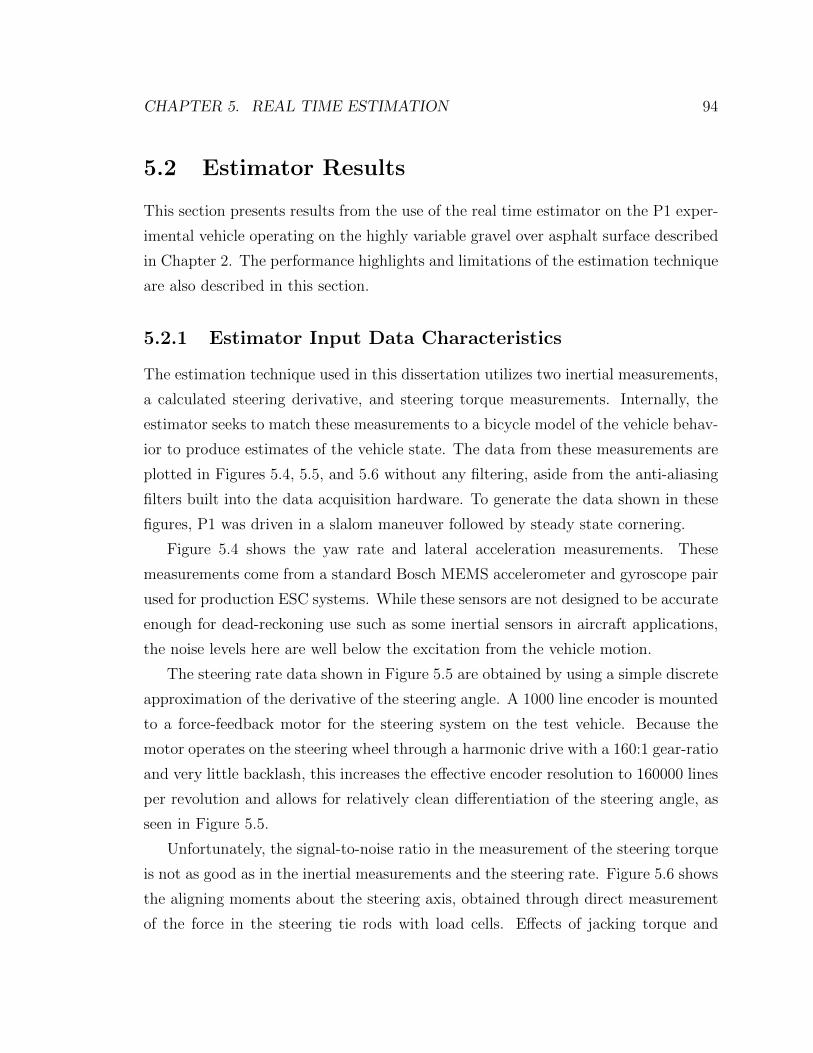
CHAPTER 5. REAL TIME ESTIMATION 94
5.2 Estimator Results
This section presents results from the use of the real time estimator on the P1 exper-
imental vehicle operating on the highly variable gravel over asphalt surface described
in Chapter 2. The performance highlights and limitations of the estimation technique
are also described in this section.
5.2.1 Estimator Input Data Characteristics
The estimation technique used in this dissertation utilizes two inertial measurements,
a calculated steering derivative, and steering torque measurements. Internally, the
estimator seeks to match these measurements to a bicycle model of the vehicle behav-
ior to produce estimates of the vehicle state. The data from these measurements are
plotted in Figures 5.4, 5.5, and 5.6 without any filtering, aside from the anti-aliasing
filters built into the data acquisition hardware. To generate the data shown in these
figures, P1 was driven in a slalom maneuver followed by steady state cornering.
Figure 5.4 shows the yaw rate and lateral acceleration measurements. These
measurements come from a standard Bosch MEMS accelerometer and gyroscope pair
used for production ESC systems. While these sensors are not designed to be accurate
enough for dead-reckoning use such as some inertial sensors in aircraft applications,
the noise levels here are well below the excitation from the vehicle motion.
The steering rate data shown in Figure 5.5 are obtained by using a simple discrete
approximation of the derivative of the steering angle. A 1000 line encoder is mounted
to a force-feedback motor for the steering system on the test vehicle. Because the
motor operates on the steering wheel through a harmonic drive with a 160:1 gear-ratio
and very little backlash, this increases the effective encoder resolution to 160000 lines
per revolution and allows for relatively clean differentiation of the steering angle, as
seen in Figure 5.5.
Unfortunately, the signal-to-noise ratio in the measurement of the steering torque
is not as good as in the inertial measurements and the steering rate. Figure 5.6 shows
the aligning moments about the steering axis, obtained through direct measurement
of the force in the steering tie rods with load cells. Effects of jacking torque and

CHAPTER 5. REAL TIME ESTIMATION 95
35 40 45 50−50
0
50
Time (s)
Yaw RateLat. Acceleration at CG
Figure 5.4: Representative Inertial Measurements
35 40 45 50−4
−2
0
2
4x 10⁻³
Time (s)
Stee
ring
Rat
e (ra
d/s)
Figure 5.5: Representative Steering Derivative
35 40 45 50−200
0
200
Left
(Nm
)
35 40 45 50−200
0
200
Rig
ht (N
m)
Time (s)
Figure 5.6: Representative Aligning Moments

CHAPTER 5. REAL TIME ESTIMATION 96
0 5 10 15 20 25 30 350
10
20
30
40
Freq
uenc
y C
onte
nt
Frequency (Hz)
Figure 5.7: Aligning Moment Frequency Content
damping have been subtracted from the measurements to remove any known torque
components not coming from the aligning moment. This figure demonstrates the
challenge in accurately estimating the quantities of interest on the variable gravel over
asphalt surface. In the slalom portion of the maneuver, the aligning moment appears
to be roughly sinusoidal with an amplitude of 100 Nm and variation of approximately
±100 Nm. In the steady state cornering phase, the data is somewhat cleaner, but
still includes quite a bit of variation.
The significant difference in the noise characteristics between the aligning moment
measurements and the inertial measurements is due, to a large extent, to the loca-
tions of the sensors. Because the load cells are attached to the steering tie rod, the
possibility of undesired excitation exists. The tie rod is attached to the wheel, which
experiences suspension modes such as the tire hop mode around 15 Hz and body
pitch and heave modes around 2 Hz. The ideal suspension model assumes that these
vertical motions are decoupled from the steering, but Figure 5.7 demonstrates that
these frequencies appear in the aligning moment measurement both at their primary
frequencies and with subharmonics and harmonics. In addition to the non-idealities
of the suspension, the location of the sensor also has a direct effect due to the small
unsprung mass. Unlike the inertial sensors, for which the excitation is limited by the
inertia of the chassis, the load cells are subject to all of the variations in force gen-
erated by the tire as it encounters different amounts of gravel on the driving surface.
One approach to handling this measurement would be to use a filter to restrict the

CHAPTER 5. REAL TIME ESTIMATION 97
frequency content in the signal, but experiments with this approach demonstrated
that the filters necessary to improve the magnitude response of the signal resulted
in phase delays that were unacceptable for use in real time control. Therefore, the
signals were left unfiltered and the signal variation was handled within the estimation
structure.
5.2.2 Slip Angle Observer Results
35 40 45 50−10
−5
0
5
10
Time (s)
Fron
t Slip
Ang
le (d
eg)
EstGPS
(a) Front Slip Angle Estimate
35 40 45 50−10
−5
0
5
10
Time (s)
Rea
r Slip
Ang
le (d
eg)
EstGPS
(b) Rear Slip Angle Estimate
Figure 5.8: Slip Angle Estimates
While the observer structure couples together the friction and front slip angle es-
timation, it is instructive to examine the two parts of the estimator separately. In the
slip angle observer, the derivative of the slip angle is calculated using only previous
estimates and the yaw rate and steering rate measurements, as seen in Eq. 5.3. As
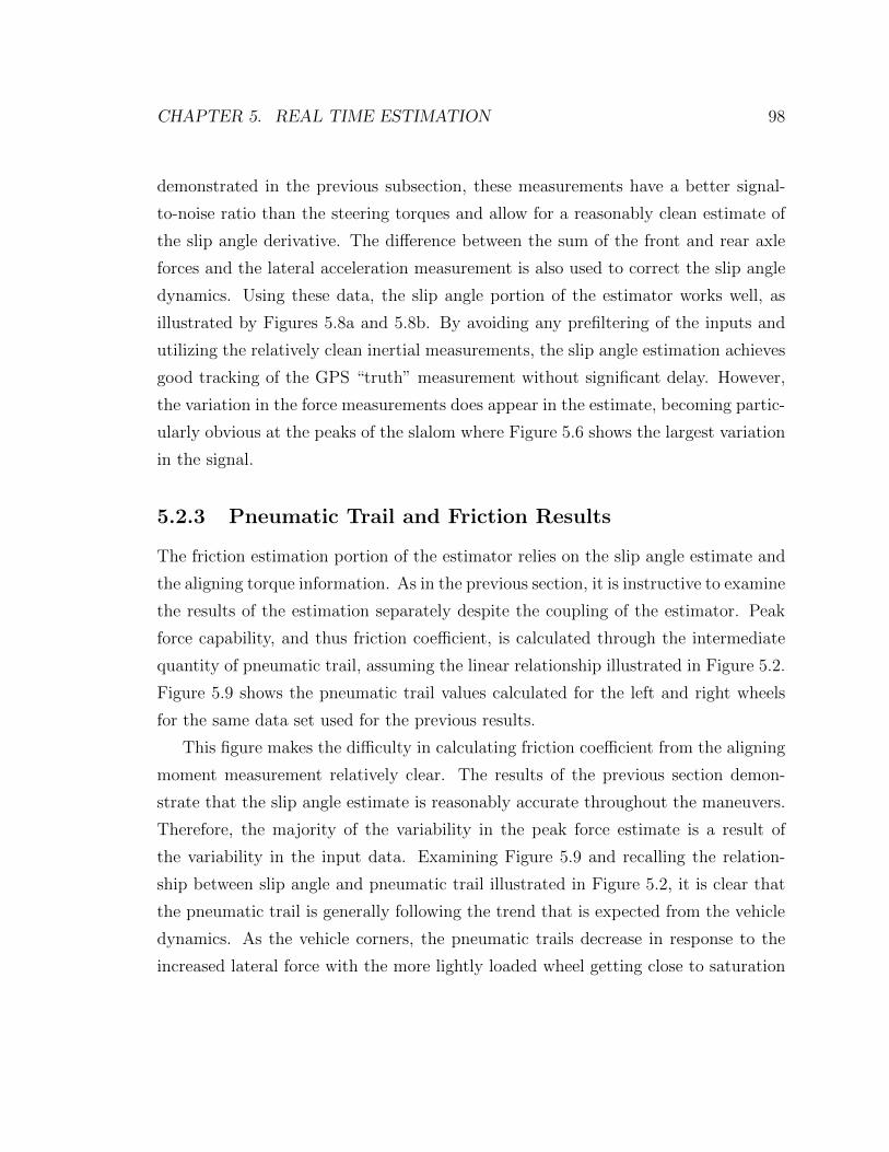
CHAPTER 5. REAL TIME ESTIMATION 98
demonstrated in the previous subsection, these measurements have a better signal-
to-noise ratio than the steering torques and allow for a reasonably clean estimate of
the slip angle derivative. The difference between the sum of the front and rear axle
forces and the lateral acceleration measurement is also used to correct the slip angle
dynamics. Using these data, the slip angle portion of the estimator works well, as
illustrated by Figures 5.8a and 5.8b. By avoiding any prefiltering of the inputs and
utilizing the relatively clean inertial measurements, the slip angle estimation achieves
good tracking of the GPS “truth” measurement without significant delay. However,
the variation in the force measurements does appear in the estimate, becoming partic-
ularly obvious at the peaks of the slalom where Figure 5.6 shows the largest variation
in the signal.
5.2.3 Pneumatic Trail and Friction Results
The friction estimation portion of the estimator relies on the slip angle estimate and
the aligning torque information. As in the previous section, it is instructive to examine
the results of the estimation separately despite the coupling of the estimator. Peak
force capability, and thus friction coefficient, is calculated through the intermediate
quantity of pneumatic trail, assuming the linear relationship illustrated in Figure 5.2.
Figure 5.9 shows the pneumatic trail values calculated for the left and right wheels
for the same data set used for the previous results.
This figure makes the difficulty in calculating friction coefficient from the aligning
moment measurement relatively clear. The results of the previous section demon-
strate that the slip angle estimate is reasonably accurate throughout the maneuvers.
Therefore, the majority of the variability in the peak force estimate is a result of
the variability in the input data. Examining Figure 5.9 and recalling the relation-
ship between slip angle and pneumatic trail illustrated in Figure 5.2, it is clear that
the pneumatic trail is generally following the trend that is expected from the vehicle
dynamics. As the vehicle corners, the pneumatic trails decrease in response to the
increased lateral force with the more lightly loaded wheel getting close to saturation

CHAPTER 5. REAL TIME ESTIMATION 99
35 40 45 50
0
0.02
0.04
Left
(m)
35 40 45 50
0
0.02
0.04
Rig
ht (m
)
Time (s)
Figure 5.9: Calculated Pneumatic Trail
as indicated by the pneumatic trail nearing zero. However, the variation in the align-
ing moment measurement can be seen in the large changes of the pneumatic trail
between the initial value, assumed to be 0.04 m, and zero. In particular, between 37
and 38 seconds, the pneumatic trails vary though nearly the full range, despite the
vehicle dynamics being significantly slower than frequency in this variation.
In order to reduce the variation in peak force, the calculated values are fed into
a moving average filter with a 300 sample window, which restricts the bandwidth
of the friction coefficient to 0.9Hz. Since the relevant yaw and sideslip vehicle dy-
namics are typically on this order, this filtering operation allows the estimator to
achieve reasonable performance from both the slip angle and friction values with-
out significantly compromising the dynamic performance of the estimation structure.
Figure 5.10 shows the estimated friction value after being filtered.

CHAPTER 5. REAL TIME ESTIMATION 100
35 40 45 500
0.5
1
Fric
tion
Coe
ffici
ent
Time (s)
Figure 5.10: Calculated Friction Coefficient
5.3 Coupled Controller/Estimator Design
The incorporation of the estimator with the model predictive envelope controller was
implemented in a straightforward manner. For real time implementation on the test
vehicle, the estimator and controller were run on separate computers, connected via
a CAN bus. The estimator was run at the 500Hz sampling rate of the primary
computer while the controller was run at 100Hz as before to allow time for the MPC
computations. Therefore, estimates of the slip angles and friction coefficient were
sent to the controller via CAN messages after every 5 time steps.
Additionally, the friction coefficient output from the estimator was passed through
a secondary selective moving average filter before usage in the envelope controller.
This 25 sample filter was updated only when the steering rate fell below a very restric-
tive threshold of 0.005 rads , which was selected by examining previous aligning moment
data and friction estimates. This criterion ensures that the friction estimates are only
averaged when the vehicle is near steady-state and the steering torque measurement
is least variable. In the interim periods, no filter update was performed, resulting in
the previous value being held until the next steady steering period. The resulting
friction estimate can be seen in Figure 5.11, where the estimate from prior to the
start of the plot time scale was held constant up to the completion of the slalom ma-
neuver and the beginning of steady-state cornering. Previous experiments with over-
and under-estimated a priori friction values suggest that the controller is capable of

CHAPTER 5. REAL TIME ESTIMATION 101
35 40 45 500
0.5
1
Fric
tion
Coe
ffici
ent
Time (s)
Figure 5.11: Calculated Friction Coefficient
handling a 20% to 30% friction mismatch. Therefore, for smooth controller action
and better passenger comfort, it was deemed better to update selectively to restrict
variation in the friction coefficient estimate.
The controller was also adapted slightly for better coupled operation with the
estimator. This adaptation is in the post-processing phase of the controller, where
a steering angle is determined from the lateral force output of the optimization. In
the controller results presented in Chapter 4, the steering angle was always chosen to
achieve exactly the desired force without allowing any significant understeer. How-
ever, this algorithm limits the achievable front slip angle, and in the case of a friction
underestimate, prevents the front axle from utilizing the full potential of the tires to
generate lateral force. This situation is made even worse by the fact that the friction
estimator cannot obtain sufficient excitation to improve the estimate while in this
situation. Therefore, in cases where the optimization output demands the maximum
lateral force, the driver input is not altered so long as the front slip angle is past the
point where the tire is fully saturated. Results later in this chapter will demonstrate
the advantage of this change in the algorithm.
5.4 Control Results with Real Time Estimation
The results presented in the previous sections demonstrate the viability of the real
time friction and slip angle estimation technique. This section presents results from
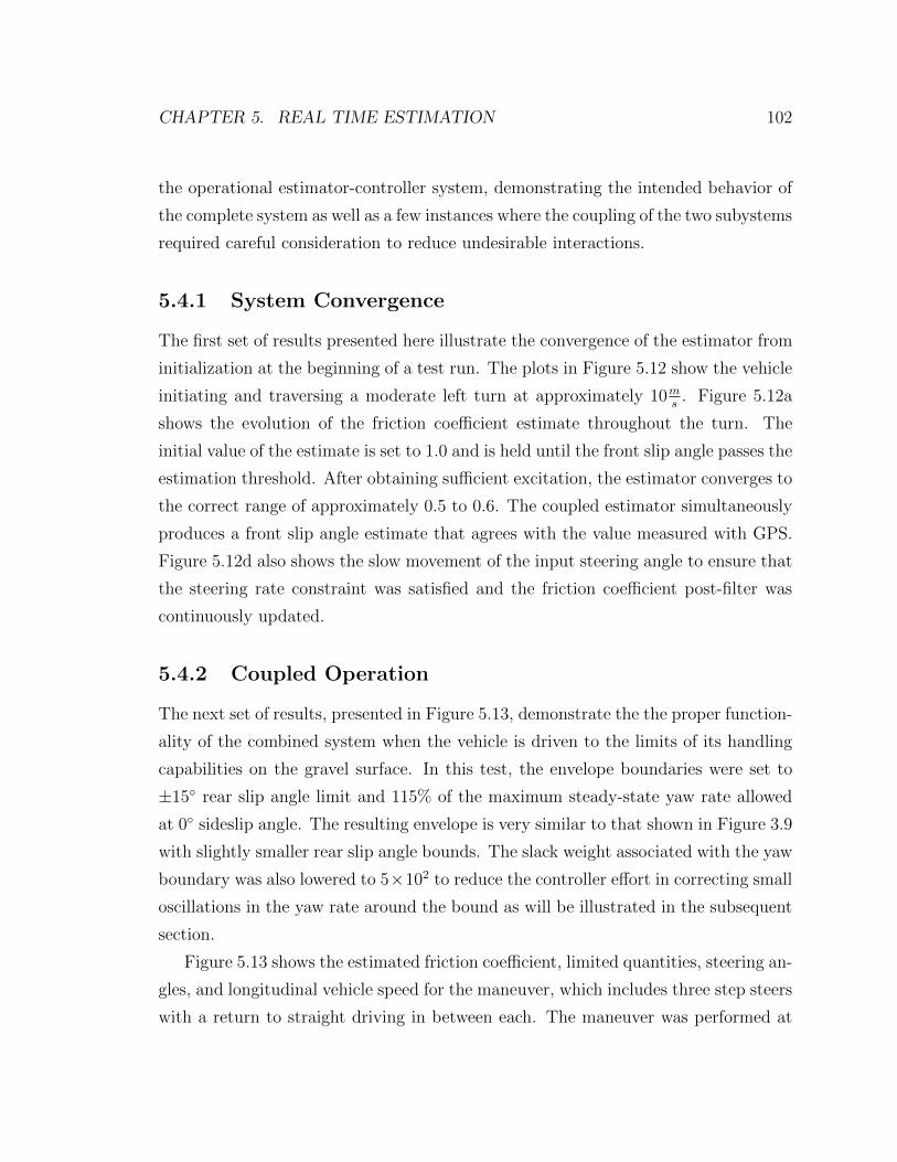
CHAPTER 5. REAL TIME ESTIMATION 102
the operational estimator-controller system, demonstrating the intended behavior of
the complete system as well as a few instances where the coupling of the two subystems
required careful consideration to reduce undesirable interactions.
5.4.1 System Convergence
The first set of results presented here illustrate the convergence of the estimator from
initialization at the beginning of a test run. The plots in Figure 5.12 show the vehicle
initiating and traversing a moderate left turn at approximately 10ms . Figure 5.12a
shows the evolution of the friction coefficient estimate throughout the turn. The
initial value of the estimate is set to 1.0 and is held until the front slip angle passes the
estimation threshold. After obtaining sufficient excitation, the estimator converges to
the correct range of approximately 0.5 to 0.6. The coupled estimator simultaneously
produces a front slip angle estimate that agrees with the value measured with GPS.
Figure 5.12d also shows the slow movement of the input steering angle to ensure that
the steering rate constraint was satisfied and the friction coefficient post-filter was
continuously updated.
5.4.2 Coupled Operation
The next set of results, presented in Figure 5.13, demonstrate the the proper function-
ality of the combined system when the vehicle is driven to the limits of its handling
capabilities on the gravel surface. In this test, the envelope boundaries were set to
±15◦ rear slip angle limit and 115% of the maximum steady-state yaw rate allowed
at 0◦ sideslip angle. The resulting envelope is very similar to that shown in Figure 3.9
with slightly smaller rear slip angle bounds. The slack weight associated with the yaw
boundary was also lowered to 5×10² to reduce the controller effort in correcting small
oscillations in the yaw rate around the bound as will be illustrated in the subsequent
section.
Figure 5.13 shows the estimated friction coefficient, limited quantities, steering an-
gles, and longitudinal vehicle speed for the maneuver, which includes three step steers
with a return to straight driving in between each. The maneuver was performed at

CHAPTER 5. REAL TIME ESTIMATION 103
20 21 22 23 24 25 26 27 28 29 300
0.5
1
Time (s)
Fric
tion
Coe
ffici
ent
(a) Estimated Friction Coefficient
20 21 22 23 24 25 26 27 28 29 30−8
−6
−4
−2
0
Time (s)
Slip
Ang
le (d
eg)
GPSEstLimits
(b) Front Slip Angle
20 21 22 23 24 25 26 27 28 29 30−0.5
0
0.5
1
Time (s)
Lim
its (r
ad,ra
d/s)
Yaw RateRear Slip AngleLimits
(c) Yaw Rate and Rear Slip with Limits
20 21 22 23 24 25 26 27 28 29 30−20
−10
0
10
20
Time (s)
Stee
ring
Angl
e (d
eg)
Driver CommandActual Angle
(d) Driver and Controlled Steering Angles
Figure 5.12: Convergence of the Friction Estimate under Envelope Control

CHAPTER 5. REAL TIME ESTIMATION 104
65 66 67 68 69 70 71 72 73 740
0.5
1
Time (s)
Fric
tion
Coe
ffici
ent
(a) Estimated Friction Coefficient
65 66 67 68 69 70 71 72 73 74−2
−1
0
1
Time (s)
Lim
its (r
ad,ra
d/s)
Yaw RateRear Slip AngleLimits
(b) Yaw Rate and Rear Slip with Limits
65 66 67 68 69 70 71 72 73 74−10
0
10
20
Time (s)
Stee
ring
Angl
e (d
eg)
Driver CommandActual Angle
(c) Driver and Controlled Steering Angles
65 66 67 68 69 70 71 72 73 740
5
10
Time (s)
Spee
d (m
/s)
(d) Vehicle Speed
Figure 5.13: Envelope Control with Real Time Slip and Friction Estimate

CHAPTER 5. REAL TIME ESTIMATION 105
10ms with cruise control, which was employed to maintain a constant speed, but also
to minimize rear wheel drive torques. Unlike the manuever presented in Figure 5.12,
in this maneuver the natural yaw and sideslip oscillations of the vehicle caused the
controller to make frequent steering corrections. Thus, the friction estimate was up-
dated less frequently as a result of the friction post filter. The estimated value is
slightly outside of the expected range between 0.5 and 0.6, likely an effect of unmod-
eled rear wheel torques that reduce lateral grip. Figure 5.13b shows that given this
friction coefficient and the real time estimates of slip angle, the yaw rate and rear
slip angle are effectively limited to the boundaries of the envelope by the steering
corrections of the controller, seen in Figure 5.13c.
5.4.3 Controller Parameter Sensitivity
Perhaps as interesting as achieving a successful integration of the controller and esti-
mator are the subtle dynamics that occur due to the coupling of the two subsystems.
One of these is the sensitivity of the controller to variation in the slip angles from
the estimator. As seen in Figure 5.8, the slip angle estimates are noisier than the
GPS-measured values, particularly at large slip angles. This makes sense given the
structure of the estimator. Because of the nonlinear relationship between force and
slip angle of a tire, a small change in estimated force near the peak of the tire curve
results in a very large change in slip angle estimate. Therefore, the estimator is highly
sensitive to variation when near the limits of the tire grip. The result is that when
large values are chosen for the yaw rate slack weight, the controller responds to this
variation by rapidly slewing the steering system. The extra actuator effort is unnec-
essary and undesired as it generates significant and uncomfortable accelerations for
the passengers and degrades the handling.
Figure 5.14 illustrates the controller behavior when the slack penalty weights for
both the yaw rate and rear slip angle are set to 5 × 10⁴ in a steady-state cornering
maneuver. All other controller parameters are the same as the previous results. As
the maneuver is initiated, the yaw rate and rear slip constraints are reached and
the controller must countersteer. However, a combination of noise in the estimates

CHAPTER 5. REAL TIME ESTIMATION 106
68 70 72 74 76 78 80 82 84−10
−5
0
5
10
Time (s)
Slip
Ang
le (r
ad)
GPSEst
(a) Estimated Front Slip Angle
68 70 72 74 76 78 80 82 84−10
−5
0
5
10
Time (s)
Slip
Ang
le (r
ad)
GPSEstLimits
(b) Estimated Rear Slip Angle
68 70 72 74 76 78 80 82 84−10
0
10
20
Time (s)
Stee
ring
Angl
e (d
eg)
Driver CommandActual Angle
(c) Driver and Controlled Steering Angles
68 70 72 74 76 78 80 82 84−2
−1
0
1
Time (s)
Lim
its (r
ad,ra
d/s)
Yaw RateRear Slip AngleLimits
(d) Yaw Rate and Rear Slip with Limits
Figure 5.14: Envelope Control Over-response with Real Time Slip and Friction Esti-mate

CHAPTER 5. REAL TIME ESTIMATION 107
and real variation in the yaw rate result in strong steering responses in the coupled
estimator-controller system. Figures 5.14a, 5.14b, 5.14c, and 5.14d demonstrate the
system response in this case. Notice that the vehicle actually remains very close to the
yaw rate and rear slip angle limits. Absent of considerations of human comfort, the
results in Figure 5.14d would seem excellent. However, the extra steering input makes
the car difficult to drive and degrades the driver’s understanding of the assistance sys-
tem behavior at the limits of handling. Furthermore, the boundaries of the envelope
are only known approximately. Therefore, softening the constraints allows the con-
troller to generally respect these approximate boundaries without over-controlling the
vehicle.
5.4.4 “Locked-low” Operating Regime
Another interesting interaction of the estimator and controller is a situation that can
occur due to an underestimation of the friction coefficient and subsequent conser-
vatism of the controller. Accurate estimates of friction coefficient may be obtained
only after the front axle reaches 30-50% of the slip angle needed to saturate the tires.
If the estimator produces a very low friction estimate and the controller enforces the
artificially low limits, the combined system may prevent the front axle from develop-
ing sufficient excitation to obtain a better estimate. This case is exacerbated by logic
in the estimator that stops estimation if the slip angles are within the range of ±2◦.
In this case, the vehicle will be restricted to very low yaw rates, as seen in Figure 5.15
which includes steady cornering and a slalom.
Figure 5.15a shows the friction estimate throughout the maneuver. Prior to the
section of the data set plotted, the friction estimate dropped low. As a result, the
estimate remains consistently low as there is insufficient excitation to improve the
estimate. This is because of the drastic controller intervention, as seen in Figure 5.15c,
where the steering angle is severely limited. Note that the controller does a good
job of maintaining the vehicle within the artificially low boundaries, even though
this results in a significant reduction of the vehicle performance compared with the
maximum possible capabilities on the driving surface.

CHAPTER 5. REAL TIME ESTIMATION 108
65 70 75 80 85 90 950
0.5
1
Time (s)
Fric
tion
Coe
ffici
ent
(a) Estimated Friction Coefficient
65 70 75 80 85 90 95−5
0
5
Time (s)
Slip
Ang
le (r
ad)
GPSEst
(b) Estimated Front Slip Angle
65 70 75 80 85 90 95
−20
−10
0
10
Time (s)
Stee
ring
Angl
e (d
eg)
Driver CommandActual Angle
(c) Driver and Controlled Steering Angles
65 70 75 80 85 90 95−0.5
0
0.5
Time (s)
Lim
its (r
ad,ra
d/s)
Yaw RateRear Slip AngleLimits
(d) Yaw Rate and Rear Slip with Limits
Figure 5.15: “Locked-low” Coupled System Operation

CHAPTER 5. REAL TIME ESTIMATION 109
The alternative logic described in Section 5.3 that allows the driver to attain large
front slip angles in cases where countersteering is not necessary can provide some
excitation to the controller. The extended yaw rate bound for the MPC envelope
also allows the front slip angle to reach higher slip angles in non-critical situations.
However, once the yaw rate or rear slip angle limits are reached, the controller will
slew the wheels into a countersteer and control the front slip angle to a small value.
Other ad-hoc solutions may be possible, including artificially ramping the friction
estimate to “feel” for higher levels of friction or providing a small offset from the real
value to provide additional excitation to the estimator.
5.5 Discussion
The results presented in this chapter, particularly Figure 5.13, demonstrate the via-
bility of a GPS-free envelope control system using low cost inertial sensors and readily
available steering torque measurements. The robustness of the model predictive en-
velope controller allows the system to handle variation in the estimator output as a
result of the rough gravel surface, while the slack weights on the yaw rate and rear
slip angle boundaries allow the controller to automatically handle small natural os-
cillations in the vehicle dynamics around the envelope boundaries without exerting
unnecessary control effort. The final system design correctly detects the lowered fric-
tion condition, adjusting the steering angle smoothly and appropriately to prevent
the vehicle from spinning out or sliding sideways.
Chapter 6
Extensions of Envelope Control
The previous chapters of this dissertation have presented a framework for developing
a driver assistance system with model predictive control that takes advantage of the
inherent structure of MPC to track the desired vehicle trajectory, provided that it
does not exceed the limitations of the vehicle’s handling capabilities. This chapter
utilizes the same conceptual framework to control the roll states of the vehicle while
attempting to the nominal planar vehicle behavior of the uncontrolled vehicle. This
structure facilitates coordination with the driver since the vehicle behaves in accor-
dance with the driver’s internal model except in extreme cases where the controller
must drastically alter the planar behavior to prevent a dangerous roll situation.
6.1 Control of Roll Dynamics
It is well known that vehicle rollovers are particularly dangerous situations for the
occupants of a vehicle. Data from the U.S. NHTSA shows that occupants in a rollover
event are more than ten times more likely to be fatally injured than in a nonrollover
accident [65]. Coupled with the fact that high-CG vehicles (Sport Utility Vehicles)
have been popular with American automotive consumers in the last decade, these
trends suggest that systems that actively control the vehicle dynamics to prevent
rollover events create significant safety benefits for consumers.
As a result of this high rate of injuries and fatalities, there has been a significant
110

CHAPTER 6. EXTENSIONS OF ENVELOPE CONTROL 111
amount of work on rollover prevention with authors focusing on varied aspects of
the problem. The Ford Motor Company has developed the Roll Stability Control
system which has been installed on select Ford Motor Company vehicles since model
year 2003 [36]. This system uses a series of estimation techniques to identify an
imminent rollover and applies a hard braking input to a single wheel to mitigate
the rollover event. Other authors such as Chen [13] and Yoon [35] have focused on
developing metrics for assessing rollover risk that are then used to trigger a specific
rollover prevention action [13, 35]. In [60], the authors even propose a scheme to
control and correct the vehicle behavior after tire lift-off has occured. In this chapter,
the model predictive control framework used for planar envelope control is adapted to
coordinate the trade-offs that must be made in the planar vehicle dynamics to control
the roll states. Using rear wheel steering and rear wheel differential drive, two different
controllers that restrict the vehicle roll rate in extreme maneuvers are developed. This
approach to choosing the optimal actuator inputs facilitates a dramatic alteration of
the vehicle roll state trajectory while maintaining the validity of the driver’s internal
model of the planar vehicle dynamics.
6.1.1 Control Approach
There are several objectives to consider in designing controllers to modify the behavior
of the roll states. The control task is a challenging one due to the fact that most
production vehicles, like the vehicles considered in this investigation, lack actuation
of the roll dynamics and thus the roll states are excited indirectly by the forces
generated by the tires. Unfortunately, this link between the planar behaviors of
the vehicle and the roll motion of the body means that certain motions that may
be desirable from a planar perspective are unobtainable without exciting potentially
dangerous roll dynamics. Yet restricting the driver’s ability to maneuver the vehicle
may be equally dangerous. As a result, a trade-off must be made in real time to
determine the least hazardous situation. Since rollover crashes are known to have
a highly elevated injury and fatality rate, the control strategy is to use all available
actuation to prevent the overturning of the vehicle, but whenever possible, minimize

CHAPTER 6. EXTENSIONS OF ENVELOPE CONTROL 112
the deviation between the driver’s intended and the vehicle’s actual behavior.
As with the planar envelope control presented in the previous chapters, a model
predictive controller offers the opportunity to express this problem in terms of con-
straints on the roll states and costs on the differences between the nominal and con-
trolled vehicle states. This allows for the system to coordinate the available actuators
in order to preserve normal handling aspects of the vehicle, relieving the driver of the
burden of controlling the vehicle in an unfamiliar regime. However, the controller
does not incorporate information about road curvature or vehicle path. Instead, the
system utilizes the driver’s input to determine proper vehicle behavior by mapping
the inputs to a linear model of the intended vehicle state trajectory. The driver is
assumed to be capable of properly tracking the lane and avoiding obstacles provided
the vehicle responds in the expected manner to the driver’s inputs. However, drivers’
internal models are typically more accurate for the planar dynamics of the vehicle
than they are for the vehicle roll states. Thus, the linear model yields a model of the
driver’s intent that is likely appropriate for a large majority of drivers and the task
of the control system is to make sure that the driver inputs are not capable of over-
turning the vehicle while minimizing deviation from the model of expected vehicle
behavior.
Unlike the planar envelope controller presented in previous chapters, the strategy
for controlling the roll dynamics of the vehicle utilizes multiple actuators. Clearly
the roll states could be restricted through the use of front steering alone, but this
would impose significant limitations on the lateral planar dynamics of the vehicle.
To mitigate this intrusion into the lateral dynamics, a second actuator is utilized
in coordination with the front steering. Rear wheel steering is one choice for this
additional actuator, while the other is independent application of acceleration and
braking torques to the left and right wheels of the vehicle. Both actuators can be
found in certain production vehicles, although the ability to brake independent wheels
is provided by standard ESC systems that are becoming standard on all production
vehicles. More importantly, both actuators affect the planar and roll dynamics in
different ways, allowing the controller to coordinate these actuators to simultaneously
restrict the roll states and track the intended planar behavior.

CHAPTER 6. EXTENSIONS OF ENVELOPE CONTROL 113
6.1.2 MPC Expression
The model underlying the control scheme is a four-state linear model incorporat-
ing single-track planar dynamics and roll dynamics. Previous work by Carlson and
Gerdes [12] showed that model predictive control of vehicle roll states is achievable in
real time by using a simplified explicit solution to the problem. The system described
in this chapter solves the model predictive control problem in real time to calculate
an optimal set of inputs to minimize deviation from the uncontrolled state trajectory
while respecting limits on the roll states and the actuators.
The controller itself is found by phrasing the problem as a linearly constrained
quadratic problem, a subset of convex optimization problems that can be solved
robustly and rapidly as described in [10]. The same framework that was introduced
for planar envelope control can be used to phrase the roll control problem. Like the
planar problem, there is a trajectory for the states that the driver intends that should
be tracked when constraints on the actuators and states are satisfies. The linear roll
model presented in Section 2.2.4 can be discretized to form the discrete state space
description (xk+1 = Adxk + Bduk, yk = Cdxk +Dduk), allowing the model predictive
control problem to be described by the following expression:

CHAPTER 6. EXTENSIONS OF ENVELOPE CONTROL 114
minimizeN�
k=1
����xkopt − xk
des
����2Wx
+N−1�
k=1
����F kyf
����2Wu
+ ηN�
k=1
����skopt����
1(6.1a)
subject to x1opt = Adxinit +Bduinit (6.1b)
xk+1opt = Adx
kopt +Bdu
kopt +Bduuser, (6.1c)
k = 1, . . . , N��u1
opt + uuser − uinit
�� ≤ uslew (6.1d)��uk+1
opt − ukopt
�� ≤ uslew, (6.1e)
k = 1, . . . , N − 1��uk
opt + uuser
�� ≤ ulim, (6.1f)
k = 1, . . . , N − 1��xk
opt
�� ≤ xlim + skopt (6.1g)
k = 1, . . . , N
skopt ≥ 0, k = 1, . . . , N (6.1h)
where the parameters for the MPC problem are listed in Table 6.1 and the optimiza-
tion variables are xkopt for time steps k = 1, . . . , N , the optimal state trajectory,
ukopt for time steps k = 1, . . . , N − 1, the optimal input addition to the user input,
and skopt for time steps k = 1, . . . , N , the slack variables on the state limits (to
prevent infeasible problems). Just as with the planar envelope control, these slack
variables remain unused (zero-valued) unless the optimization problem is infeasible.
In this expression of the problem, both the roll angle and roll rate are constrained,
though the limits may be set so that either one of these constraints is never active in
operation.

CHAPTER 6. EXTENSIONS OF ENVELOPE CONTROL 115
Table 6.1: Description of Roll Controller Parameters
Parameter Description
Ad Discrete State Propagation Matrix
Bd Input Effect Matrix
Wx State Tracking Weight Matrix
Wu Input Penalty Matrix
xdes Open Loop Trajectory from Driver Input
xinit Vehicle State at Start of Optimization
uinit Vehicle Actuator State at Start of Optimization
uuser Driver Commanded Input (constant over the horizon)
xlim State and Input Limits
ulimits Actuator Saturation Limits
uslew Limit on Rate of Change of Inputs
η Stiffness of Slack Variables
6.1.3 Real Time MPC Implementation
Typically a MPC problem is solved at every time step to find an optimal input
sequence from which only the first calculated input is utilized. However, the com-
putation time for this problem is non-negligible and an input may not be calculated
rapidly enough for the immediate time step. Instead, the input for the following time
step is calculated, stored, and applied at the appropriate time. The input parameters
can be varied between time steps. Thus, the controller limits can be computed in real
time or adjusted with adaptive techniques.
To solve the MPC problem, the same convex optimization tools used for the
planar envelope controller may be applied. This toolchain, CVXMOD [44], produces
automatically generated C-code that can solve this roll control problem in less than
10 milliseconds on a modern Pentium processor chip. This is slightly longer than the
results observed for the planar problem, which can be attributed to the additional
states and dynamics required to describe the roll motion of vehicle.
CHAPTER 6. EXTENSIONS OF ENVELOPE CONTROL 116
The work done on this rollover prevention technique examines the possibility of
using either rear differential drive or rear wheel steering to provide a needed additional
degree of freedom to the base mode of the vehicle. The P1 experimental steer- and
drive-by-wire research vehicle, described in Chapter 2 and shown in Figure 2.7, is
equipped with independent drive motors for the rear wheels and has the capability to
support testing of the differential drive concept. The rear wheel steering concept can
be tested on a different platform, referred to as X1, that has also been developed by
students in the mechanical engineering department at Stanford University. The X1
by-wire vehicle couples a modular chassis design with a distributed data collection
and control system based on the Flexray communication standard and can be seen
in Figure A.1. A more complete description of X1 can be found in Appendix A.
6.2 Simulation Results
6.2.1 Roll Control Objective
A number of criteria for preventing vehicle rollover events have been presented in
previous publications. These include static stability criteria, time-to-rollover metrics,
roll angle limits, and wheel lift criteria [68, 13, 35, 36]. The model predictive controller
described in this chapter provides the mechanism for describing a linear limitation of
the roll rate and roll angle. Since most production vehicles will lose tire grip before
rolling over in a static manuever, as demonstrated by the NHTSA rollover testing
[68], it is assumed that non-tripped rollovers are caused by dynamic maneuvers such
as the fish hook and J-turn that excite both large roll rates and roll angles. Therefore,
the results presented in this section describe the vehicle behavior when the roll rate
is restricted as an illustration of the potential of this assistance scheme.
6.2.2 Baseline Dynamics
As a baseline for the discussion of the results in this section, the uncontrolled vehicle
behavior was examined in simulation using the nonlinear yaw-roll model to describe
the vehicle behavior. This model, described in Section 2.2.1, includes degrees of

CHAPTER 6. EXTENSIONS OF ENVELOPE CONTROL 117
0 0.5 1 1.5 2−0.1
0
0.1
0.2
0.3
0.4
Time (s)
Stat
es (r
ad, r
ad/s
, rad
, rad
/s)
Yaw RateRoll RateRoll AngleSideslip AngleUncontrolled States
(a) Nominal States
0 0.5 1 1.5 2
0
1
2
3
4
Time (seconds)
Stee
ring
angl
e (d
eg)
Driver commandTotal command
(b) Steering Input
Figure 6.1: Vehicle State and Input Trajectories for Baseline (Inactive) Case
freedom for yaw rate, sideslip angle, roll angle, roll rate, and independent wheel
dynamics for all four wheels. A nonlinear brush tire model such as the one described
in Section 2.1.1 was used to calculate the tire forces. Later simulations demonstrate
the ability of the controller to restrict the roll rate to 0.15 rads and 0.18 rad
s , but in
this case no restriction is specified and so the figures illustrate the nominal dynamics
for the roll rate and roll angle of the uncontrolled vehicle. This case can be seen in
Figure 6.1.
The driver’s steering input for this simulation was generated by applying a 3Hz
low-pass filter to a 3.5 degree fast ramp steer input. This filtering represents the
limited capability that a human possesses to create extremely fast steering inputs.
Data taken from research testbeds under manual driving supports the observation
that nearly all of the frequency content of a driver’s input signal is at or below 3Hz.
Since the vehicle model incorporates the assumption that the vehicle travels at a
constant speed, a “cruise control” function was used to keep the vehicle at 20 m/s
for the duration of the maneuver.

CHAPTER 6. EXTENSIONS OF ENVELOPE CONTROL 118
0 0.5 1 1.5 2−0.1
0
0.1
0.2
0.3
0.4
Time (s)
Stat
es (r
ad, r
ad/s
, rad
, rad
/s)
Yaw RateRoll RateRoll AngleSideslip AngleUncontrolled States
Figure 6.2: Vehicle State Trajectories for Drive/Brake Torque Controller
0 0.5 1 1.5 2
0
1
2
3
4
Time (seconds)
Stee
ring
angl
e (d
eg)
Driver commandTotal command
(a) Front steering angles
0 0.5 1 1.5 2
−1000
−500
0
500
1000
Time (seconds)
Torq
ue (N
m)
Left rear wheelRight rear wheel
(b) Rear wheel torques
Figure 6.3: Inputs for Controlled Fast Ramp Steer with Differential Drive

CHAPTER 6. EXTENSIONS OF ENVELOPE CONTROL 119
Table 6.2: Independent Wheel Torque Roll Controller Parameters
Parameter Symbol Value Units
roll angle limit xlim[1] ±10 deg
roll rate limit xlim[2] ±0.18 rad/s
front steer limit ulim[1] ±20 deg
wheel torque limit ulim[2] ±1370 Nm
torque slew limit uslew[1, 2] ±24000 Nm/s
slack penalty η 106 –
time horizon N 15 –
6.2.3 Independent Wheel Torque Control
The first controlled case is the drive-brake controller, which uses independent control
of the accelerating and braking torques on the rear wheels to complement the front
steering actuator to achieve a restriction of the roll rate to 0.18 rads . This roll rate was
selected by examining the nominal dynamics of the vehicle and choosing a limit that
would require significant controller intervention to achieve while still retaining much
of the nominal vehicle behavior. Table 6.2 lists the full set of controller parameters
used for the simulation.
The state trajectories as well as front steering and rear torque commands for the
system under control of the drive-brake controller can be seen in Figures 6.2 and 6.3,
respectively. In Figure 6.2, there is clearly a significant deviation from the nominal
yaw rate trajectory. Examining Figure 6.3, there is a significant steering correction to
control the roll rate while the rear-wheel torque saturates to the limits set to represent
the maximum longitudinal force that the rear tires can produce. Despite saturating
the longitudinal forces on the rear axle, the controller is unable to compensate for
the yaw rate lost by reducing the front steering. This is a result of the geometry of
the car and the coupling of the lateral and longitudinal forces. Because the width of
the car is smaller than the length, very large differential longitudinal forces must be
created to generate effective yaw moments. However, because of the coupled nature

CHAPTER 6. EXTENSIONS OF ENVELOPE CONTROL 120
of lateral and longitudinal force generation by the tires, large torques may not result
in the desired longitudinal force, particularly if the vehicle is cornering agressively.
This reduces the effectiveness of differential torques as a means to regulate the roll
dynamics of the vehicle.
In addition to the physical limitation of the independent torques, the coupled tire
forces are challenging to represent in a convex formulation that is suitable for express-
ing as part of the model predictive control problem. Therefore, a linear model was
utilized, along with a 100Hz sample rate was that was expected to compensate for
some of the reduction in the accuracy of the model. Thus, the nonlinear simulations
presented here demonstrate the level of impact on the system due to the controller
modeling assumptions. Despite having a linear model that leaves out this force cou-
pling, the feedback aspect of model predictive controller is capable of controlling the
roll rate. However, it is at the expense of tracking the yaw rate trajectory. Further
reductions in the roll rate limit below 0.18 rads result in significantly worse tracking of
the yaw rate.
6.2.4 Rear Wheel Steering Control
The second controller is a front- and rear-wheel steering controller. This controller
was also simulated with the same nonlinear model and driver inputs used for the
drive-brake controller. The state trajectories as well as front- and rear-wheel steering
commands for the system can be seen in Figures 6.4 and 6.5, respectively. Note that
in this example, the roll rate limit was lowered to 0.15 rad/s to demonstrate the
performance of the controller in a case where the limit more significantly restricted
the nominal vehicle dynamics. Table 6.3 lists the full set of controller parameters
used for the simulation.
The behavior of the controlled system is improved when compared to the perfor-
mance of the system when using the differential wheel torque actuator. In this case,
the roll rate constraint is met and modification of the roll states results in significantly
less degradation of the tracking of the uncontrolled system trajectory.
Like the differential torque controller, the necessary reduction in lateral force to

CHAPTER 6. EXTENSIONS OF ENVELOPE CONTROL 121
Table 6.3: Rear Steering Roll Controller Parameters
Parameter Symbol Value Units
roll angle limit xlim[1] ±10 deg
roll rate limit xlim[2] ±0.18 rad/s
front steer limit ulim[1] ±20 deg
rear steer limit ulim[2] ±10 deg
steer slew limit uslew[1, 2] ±140 deg/s
slack penalty η 106 –
time horizon N 15 –
keep the roll rate within the limit is accomplished by reducing the front steering
angle, which, if performed as the only action, would cause a decrease in yaw rate.
However, the model predictive control scheme can coordinate the rear steering as well,
and so the controller compensates for the reduction in the front steering angle by an
increase in the magnitude of the rear steering angle to increase the yaw moment. The
slight oscillation seen in Figure 6.5 is a result of the driver input changing in between
subsequent controller time steps. As the driver changes the angle of the steering
wheel, the controller must adjust both to the changed desired trajectory and also the
resulting dynamics.
The results of the simulations demonstrate that the front and rear steering con-
troller is more effective in controlling the roll rate while matching the yaw rate and
sideslip trajectories of the vehicle. As seen in Figure 6.5, the required steering mod-
ifications to the front and rear of the vehicle are on the order of ±1◦, whereas the
front and rear physical steering limits are ±30◦ and ±20◦, respectively. These small
magnitude corrections illustrate that standard rear-steering systems such as those
seen on a few recent production vehicles have sufficient actuator authority to signifi-
cantly influence the roll states of the vehicle if coordinated with front steering angle
corrections.

CHAPTER 6. EXTENSIONS OF ENVELOPE CONTROL 122
The simulations presented here highlight the value of the model predictive con-
troller, as the roll states are significantly modified while degradation of the planar
vehicle behavior is minimized. This ensures that the actions of the controller pre-
serve the validity of the driver’s model of the vehicle behavior, enabling the driver
to handle the tasks of lanekeeping and obstacle avoidance. Additionally, it is clear
that the magnitude of the steering corrections remain small when using rear-wheel
steering as a second actuator, minimizing modeling error and maximizing controller
performance.
0 0.5 1 1.5 2−0.1
0
0.1
0.2
0.3
0.4
Time (s)
Stat
es (r
ad, r
ad/s
, rad
, rad
/s)
Yaw RateRoll RateRoll AngleSideslip AngleUncontrolled States
Figure 6.4: Vehicle State Trajectories for Rear Wheel Steering Controller

CHAPTER 6. EXTENSIONS OF ENVELOPE CONTROL 123
0 0.5 1 1.5 20
0.5
1
1.5
2
2.5
3
3.5
4
Time (seconds)
Fron
t ste
erin
g an
gle
(deg
)
Driver commandTotal command
(a) Front steering angles
0 0.5 1 1.5 2−0.8
−0.6
−0.4
−0.2
0
0.2
Time (seconds)
Rea
r ste
erin
g an
gle
(deg
)
Driver commandTotal command
(b) Rear steering angles
Figure 6.5: Inputs for Controlled Fast Ramp Steer with Rear Wheel Steering
6.3 Discussion
In this chapter, a pair of controllers designed to coordinate the actions of different
actuator sets for control of vehicle roll rate were presented. While both controllers
successfully coordinated the vehicle actuators to respect the roll state limits, the
deviation in the planar state tracking was significantly lower using a front- and rear-
wheel steering controller than using rear-wheel drive and braking to augment front
steering control.
The nonlinear simulation also demonstrates that the rear-wheel drive/brake con-
troller must exert very large rear-wheel torques to achieve the desired result, which
result in negative effects when considering the real pneumatic tire with coupled lon-
gitudinal and lateral forces. The four-wheel steering controller, however, uses very
small steering corrections at each axle. Thus, the linear model used for the controller
yields a more accurate representation of the vehicle behavior and results in better
controller performance.
Despite the different dynamics involved in controlling the roll states of the vehicle,
these controllers demonstrate the validity of the model predictive control framework
used for both planar envelope and roll control. When phrased as a problem of tracking

CHAPTER 6. EXTENSIONS OF ENVELOPE CONTROL 124
the driver’s desired vehicle behavior while incorporating limits on the vehicle handling,
this structure allows the controller to appropriately incorporate the driver’s input.
The result is a driver assistance system that can operate in tight collaboration with
a driver to make a vehicle safer in highly adverse conditions.

Chapter 7
Conclusions
The work presented in this dissertation demonstrates the feasibility of using real time
estimates of friction and vehicle sideslip angle to assist drivers in stabilizing the vehicle
at the limits of handling. The system, unlike production stability control systems,
allows the driver complete freedom to maneuver the vehicle within the bounds of a
safe handling envelope.
7.1 Summary
This dissertation presents a number of new concepts, summarized in the following
subsections by chapter.
7.1.1 Safe Handling Envelopes
Chapter 3 presents a method for finding a safe handling envelope. Once the tire-road
friction coefficient and the speed are known, the method allows for the calculation of
an envelope in terms of the planar vehicle states. The physically motivated boundaries
of this envelope can be continuously updated in real time and offer the driver access
to a significant portion of the state space. For intrepid drivers who are comfortable
driving with the rear tires in a saturated condition, the boundaries of the handling
envelope can be expanded to allow for high sideslip “drifting” maneuvers.
125

CHAPTER 7. CONCLUSIONS 126
7.1.2 Real Time Model Predictive Control
Chapter 4 presents a model predictive envelope controller that enforces the boundaries
of the safe handling envelopes in real time. The development of the controller includes
the formulation of the Affine Force-Input model, a critical step in generating a problem
that can be solved with convex optimization techniques in real time at 100Hz. The
resulting controller yields smooth, progressive, and predictive augmentations to the
driver’s steering input to stabilize the vehicle while allowing it to reach the maximum
extents of the safe handling envelope.
7.1.3 Real Time Friction and Sideslip Estimation
In order to implement the envelope controller in a production vehicle, sensing of the
friction coefficient and vehicle sideslip angle are needed in real time. Because it is
difficult to obtain measurements of these quantities with inexpensive sensors, Chapter
5 describes the implementation of an estimation technique that utilizes steering torque
measurements to supplement readily available inertial sensors to provide the necessary
information to the envelope controller. Despite guarantees of stability of the two
separate algorithms, the coupling of the controller and estimator sometimes led to
poor system performance in experimental testing. The reasons for these performance
issues are analyzed and several solutions to this problem are introduced.
7.1.4 Extension of the Envelope Control Technique
The envelope controller presented in this dissertation is designed to control the pla-
nar states of the vehicle. Yet there are other vehicle control problems that can be
phrased in terms of driver intent that must be limited by a safe envelope. The model
predictive envelope control technique may be extended to handle many of these prob-
lems. Chapter 6 presents a controller of the same model predictive control form that
is used to coordinate multiple vehicle actuators to prevent the vehicle roll states from
exceeding the bounds of a safe envelope.

CHAPTER 7. CONCLUSIONS 127
7.2 Future Work
This dissertation has demonstrated that the model predictive envelope controller
yields good performance in conjunction with the human driver, and that control of the
front steering of the vehicle in response to the friction conditions in the environment
can rapidly and smoothly stabilize the vehicle. However, there are a few key areas in
which this work may be extended and improved.
7.2.1 Driver Feedback
In the discussion in Chapter 5, the issue of informing the driver of the controller
action was briefly addressed. In experimental testing, it was noted by several drivers
that it often felt like the vehicle dramatically understeered, particularly with cer-
tain controller settings. In many of these cases, the vehicle was actually doing just
the opposite and tending toward oversteer, but the controller was countersteering to
prevent a spin. Thus, the drivers were merely misunderstanding the control action.
Developing haptic feedback to inform the driver of the augmented steering command
would likely improve the interpretation by the driver and lead to better acceptance
of the system by drivers.
7.2.2 Controller Complexity
The model predictive envelope controller presented in this dissertation is an optimal
control design for a particular set of specified criteria. However, a relatively powerful
computer is required to solve the problem in real time on the vehicle. At present,
ruggedized computers suitable for installation in a vehicle are expensive and lack the
speed needed for the control computations. However, using the phase-plane analysis
presented in Chapter 3, other less computational techniques for controlling the han-
dling dynamics could be compared to the model predictive controller to develop a
controller suitable for use in currently available production hardware.

CHAPTER 7. CONCLUSIONS 128
7.2.3 Handling Environmental Constraints
The safe handling envelopes presented in Chapter 3 are calculated based on estimates
of the maximum vehicle performance. When the controller enforces these boundaries,
there are cases in which the driver steers to travel through a corner but the controller
limits the minimum radius of the corner that the vehicle can achieve. When the
envelope is calculated correctly, the controller is not “taking away” performance, but
rather the driver’s intended path is unachievable. In this case, a new path that is
achievable must be selected, either by the driver or by the controller.
The action of the current model predictive controller is to maintain the minimum
radius corner since the objective of the controller is to match the intent of the driver.
However, a different formulation of the control objective might be to find and traverse
a safe trajectory, regardless of driver input. This would be a significant departure
from the intent of the current controller, yet it would be possible to use additional
information about obstacles and the environment to choose a safer alternative path.
Integration of environmental sensing would also allow for prediction of infeasible tra-
jectories and the ability to keep the vehicle out of these hazardous situations. Despite
the different objectives of these controllers, the control framework presented in this
dissertation may be used as a foundation upon which to base the development of this
new control design.
7.3 Outlook
The envelope control approach to assisting drivers in stabilizing a vehicle shows great
promise. The additional information provided to the controller by the friction and
sideslip estimation technique yields a controller that allows a skilled driver to utilize
the maximum handling capabilities of the vehicle. There are, of course, a number
of challenges in refining the system to the point of being ready for installation in
production cars, but this dissertation demonstrates the advantages of the system.
Additionally, hybrid and electric cars and the use of electric motors to actuate steer-
ing systems are becoming increasingly common, providing the opportunity for tighter

CHAPTER 7. CONCLUSIONS 129
control and additional driver assistance over all aspects of the driving experience.
These new opportunities for control can allow the designers of driver assistance to
develop seamless systems that allow even the most intrepid drivers to enjoy the ex-
perience of driving, knowing that somewhere under the hood is a controller to keep
them safe.

Appendix A
X1 Experimental Test Vehicle
The X1 experimental test vehicle is an electric vehicle designed and constructed by
students at Stanford University. This vehicle leverages electronic and physical modu-
larity to allow for adaptation to changing research needs and the creation of student
projects focused on particular subsystems of the vehicle.
A.1 Physical Design
X1 was designed with the research needs and manufacturing capabilities of students
at the Dynamic Design Lab in mind. Because the construction of large body panels
with complex geometries was incompatible with the available fabrication equipment,
the structure of the chassis was designed not only to provide strength and rigidity,
but also to suggest the form of the car. However, this was not the only consideration,
as the safety of students operating X1 for vehicle dynamics is paramount in all testing
situations. Therefore, the chassis was also designed to protect the occupants in case
of an impact or rollover. The final vehicle design, as seen in Figure A.1, includes a
full roll cage, achieves an estimated 10000ft−lbfdeg , and suggests the shape of a car body,
satisfying the design objectives.
130

APPENDIX A. X1 EXPERIMENTAL TEST VEHICLE 131
Figure A.1: X1 Steer and Drive By-Wire Research Testbed
A.1.1 Modularity Concept
In the design phase of the vehicle, the meaning of modularity was discussed at length
and many different concepts of “modular design” were generated. Ultimately, the
driving force behind the design was determined to be maximum utility for vehicle
dynamics research. Therefore, the modules were defined such that there is a chassis
module along with front and rear suspension modules. With this definition of the
modularity, projects that seek to use different actuators such as active suspension,
steer-by-wire, active camber, or independent drive can all be accomodated with min-
imal changes to the remainder of the system. Supporting this modularity concept is
a by-wire design that limits the connections to each suspension module to a power
bus, a communication bus, and a dry-disconnect hydraulic braking line. Thus, aside
from these three connections, each module is an isolated system that can be designed,
constructed, and tested independently before installation on the vehicle.

APPENDIX A. X1 EXPERIMENTAL TEST VEHICLE 132
Figure A.2: Front-Middle-Rear Modularity Concept
Figure A.3: CAD Mockup of Modular Structure

APPENDIX A. X1 EXPERIMENTAL TEST VEHICLE 133
A.1.2 Actuation Opportunities
In designing X1 to be modular, the intent was to create as many opportunities to
alter the actuation scheme of the vehicle as possible. Therefore, the first front and
rear modules built for the vehicle are based on a double A-arm pushrod suspension
that leaves room in the module for a drive system and motors to implement steer-by-
wire. By utilizing the pushrod to locate the spring and shock remotely, this design
also includes a rotational joint upon which a motor could be mounted to actuate
the suspension. Furthermore, work done by Laws [39] was based on the X1 modu-
lar architecture and demonstrated that a suspension capable of actively controlling
camber, steering, and vertical load can be installed on the vehicle.
A.1.3 Drivetrain
The drive system selected for X1 is a battery-powered DC brushless motor obtained
from UQM Technologies. The motor is rated for 75 kW of power and 240 Nm of torque
and can be driven up to 8000 RPM. Rather than include the additional mechanical
complexity of a transmission, the motor is coupled directly to a custom fabricated
Ford 9” differential geared with a 7.33:1 ring and pinion, providing all of the gear
reduction necessary for the drivetrain. With the gearing selection, the vehicle is
capable of approximately 80 MPH before reaching the limit of the motor speed. This
direct-drive design also saves space and weight, a critical consideration since it is
desirable to locate the motor directly in the driven module. The UQM motor also
provides a research advantage in that it communicates with the vehicle through the
CAN communication protocol and reports real time measurements of battery pack
voltage, battery current draw, motor RPM, and motor torque. The input to the
motor can also be set up to accept torque or speed commands, allowing higher level
vehicle dynamics controllers such as the model predictive envelope controller to utilize
torque measurements and output torque commands.

APPENDIX A. X1 EXPERIMENTAL TEST VEHICLE 134
A.2 Electrical Design
The electrical design of the vehicle is comprised of two parts. The first is the power
system for the electric drive and the second is the electronics architecture that allows
the modules to be controlled through a data network.
A.2.1 Power System
There are a number of considerations for an electric vehicle power system. The first
is the ability of the system to supply energy to the electric motor, particularly the
total energy storage capacity. However, it is also important to consider the maximum
current that the system can source. Furthermore, it is important to choose a system
that provides relatively easy and robust charging. For this reason, the high voltage
system for X1 is comprised of 28 lead acid batteries. While this battery chemistry
does not have the highest energy density of all the technologies on the market, the
batteries can supply very large currents and are significantly more tolerant of deep
discharge and rapid charging than other battery chemistries. The batteries are also
complemented with a pair of onboard chargers capable of charging at a rate of 3.3 kW
each. The nominal charged voltage of this system is approximately 360V, allowing
for a significant power draw with lower currents than other low voltage systems.
A.2.2 Data Network
The electronic modularity of the vehicle is based on a data network implemented
with the state-of-the-art Flexray communication protocol [5]. Flexray offers several
advantages over previous vehicle communication protocols such as CAN, LIN, and
pure parallel wiring harnesses. With Flexray, redundancy in the network is easily
accomplished and large data packets containing many tens of bytes may be sent from
node to node. Furthermore, the protocol includes a time-triggered scheme for high
priority information to be sent between nodes. The ability to send multiple floating
point numbers between nodes with guaranteed latency opens up the possibility of
distributed computing on the vehicle, and supports the independence of each module.

APPENDIX A. X1 EXPERIMENTAL TEST VEHICLE 135
70
6 Implementation of the Chosen System
Based on the draft of the controller network described before, this chapter demonstrates
the implementation of the chosen system. Figure 6.1 illustrates the basic association of the
logical system structure and the real vehicle hardware. This first step in the development
Figure 6.1: Association of logical and hardware modules
process includes three logical and mechanical modules. Each of the mechanical axle modules
highlighted in figure 6.1 is assigned one controller that reads the sensors and sends reference
Figure A.4: Electronic Modularity Concept
A.3 Discussion
With the mechanical and electrical modularity of the system, the X1 test vehicle pro-
vides an excellent platform for vehicle dynamics research. The chassis is safe, flexible,
and will evolve with the research of the Dynamic Design Lab. Finally, the ability to
distribute computing load across various modules will allow for the development of
future advanced vehicle controllers such as the one presented in this thesis.

Bibliography
[1] Bosch Automotive Handbook, 6th Edition. SAE Society of Automotive Engineers,
Inc, 2004.
[2] Guillaume Baffet and Ali Charara. An observer of tire-road forces and friction
for active security vehicle systems. IEEE/ASME Transactions on Mechatronics,
12(6), 2007.
[3] Craig E. Beal and J. Christian Gerdes. Enhancing Vehicle Stability through
Model Predictive Control. In Proceedings of the ASME Dynamic Systems and
Controls Conference, September 2009.
[4] Craig E. Beal and J. Christian Gerdes. Experimental Validation of a Linear
Model Predictive Envelope Controller in the Presence of Vehicle Nonlinearities.
In Proc. of the 2010 IFAC Symp. on Advances in Automotive Control, Munich.,
July 2010.
[5] Peter Bergmiller. Design and implementation of a controller network for a mod-
ular by-wire vehicle for safety-critical real-time applications. Master’s thesis,
Technical University of Braunschweig, 2008.
[6] J. E. Bernard, L. Segel, and R. E. Wild. Tire shear force generation during
combined steering and braking maneuvres. SAE World Congress, 1977. Paper
number 770852.
[7] D. Bernardini, S. Di Cairano, Alberto Bemporad, and H.E. Tseng. Drive-by-wire
Vehicle Stabilization and Yaw Regulation: a Hybrid Model Predictive Control
136

BIBLIOGRAPHY 137
Design. In Proceedings of the 48th IEEE Conference on Decision and Control,
Shanghai, China, December 2009.
[8] David M. Bevly, Robert Sheridan, and J. Christian Gerdes. Integrating INS
sensors with GPS velocity measurements for continuous estimation of vehicle
sideslip and tire cornering stiffness. In Proceedings of the 2001 American Control
Conference (ACC), Arlington, Virginia, 2001.
[9] Francesco Borrelli, Jahan Asgari, Hongtei Eric Tseng, and Davor Hrovat. Pre-
dictive Active Steering Control for Autonomous Vehicle Systems. IEEE Trans-
actions on Control Systems Technology, 15(3), May 2007.
[10] Stephen Boyd and Lieven Vandenberghe. Convex Optimization. Cambridge
University Press, Cambridge, UK, 2004.
[11] CarAdvice.com.au. Electronic stability control getting more popular, August
2007.
[12] C. R. Carlson and J. C. Gerdes. Optimal rollover prevention with steer by wire
and differential braking. In IMECHE03, 2003.
[13] Bo-Chiuan Chen and Huei Peng. A real-time rollover threat index for sports
utility vehicles. In Proceedings of the American Control Conference (ACC), San
Diego, California, June 1999.
[14] Andy Chuter. Airbus launches more safety aids. Flight International, page 26,
1997.
[15] John Croft. Taming loss-of-control: Solutions are elusive. Aviation Week &
Space Technology, 157(9):50, August 2002.
[16] Jennifer N. Dang. Statistical analysis of the effectiveness of electronic stability
control systems. Technical report, NHTSA, July 2007.
[17] Moritz Diehl, Hans Joachim Ferreau, and Niels Haverbeke. Nonlinear Model
Predictive Control. Springer Berlin/Heidelberg, 2009.

BIBLIOGRAPHY 138
[18] Howard Dugoff, P.S. Fancher, and Leonard Segel. An analysis of tire traction
properties and their influence on vehicle dynamic performance. In Proceedings
of the SAE World Congress, Paper 700377. 1970.
[19] P. Falcone, F. Borrelli, H. E. Tseng, J. Asgari, and D. Hrovat. Linear time-
varying model predictive control and its application to active steering systems:
Stability analysis and experimental validation. International Journal of Robust
and Nonlinear Control, 6:862–975, July 2007.
[20] E Fiala. Lateral forces on rolling pneumatic tires. In Zeitschrift V.D.I. 96. 1954.
[21] Michael Gipser. Ftire : a physically based application-oriented tyre model for
use with detailed mbs and finite-element suspension models. Vehicle System
Dynamics, 43(Supplement):76–91, 2005.
[22] Havard Fjaer Grip, Lars Imsland, Tor A. Johansen, Thor I. Fossen, Jens C.
Kalkkuhl, and Avshalom Suissa. Nonlinear vehicle velocity observer with road-
tire friction adaptation. Proceedings of the 45th IEEE Conference on Decision
& Control, San Diego, CA, 2006.
[23] Fredrik Gustafsson. Monitoring tire-road friction using the wheel slip. IEEE
Control Systems Magazine, pages 42–49, 1998.
[24] R. Hadekel. The mechanical characteristics of pneumatic tyres. In S and T
Memo TPA3/TIB. 1952.
[25] S. P. Han and O. L. Mangasarian. Exact penalty functions in nonlinear pro-
gramming. Mathematical Programming, 17:251–269, 1979.
[26] Junjie He, David A. Crolla, Martin C. Levesley, and Warren J. Manning. Inte-
grated chassis control through coordination of active front steering and intelligent
torque distribution. In Proceedings of the 2004 International Symposium on Ad-
vanced Vehicle Control, Arnhem, Netherlands., August 2004.

BIBLIOGRAPHY 139
[27] P. Helnwein, C. J. Lie, G. Meschke, and H. A. Mang. A new 3-D finite element
model for cord-reinforced rubber composite: application to analysis of automo-
bile tires. Finite elements in analysis and design, 14(1):1–16, 1993.
[28] Rami Y. Hindiyeh and J. Christian Gerdes. Equilibrium Analysis of Drifting
Vehicles for Control Design. In Proceedings of the ASME Dynamic Systems and
Controls Conference, 2009.
[29] Yutuka Hirano and Katsumi Fukatani. Development of robust active rear steering
control. In Proceedings of the 1996 International Symposium on Advanced Vehicle
Control, Aachen, Germany., June 1996.
[30] Robert C. Hoffman, Jeffrey L. Stein, Loucas S. Louca, and Kunsoo Huh. Using
the milliken moment method and dynamic simulation to evaluate vehicle stability
and controllability. In Proceedings of the International Mechanical Engineering
Congress and Exposition, Anaheim, CA, November 2004.
[31] Y.-H.J. Hsu, S.M. Laws, and J.C. Gerdes. Estimation of tire slip angle and
friction limits using steering torque. Control Systems Technology, IEEE Trans-
actions on, 18(4):896–907, July 2010.
[32] Yung-Hsiang Judy Hsu and J. Christian Gerdes. The predictive nature of pneu-
matic trail: Tire slip angle and peak force estimation using steering torque.
In Proceedings of the International Symposium on Advanced Vehicle Control
(AVEC), Kobe, Japan, October 2008.
[33] Yung-Hsiang Judy Hsu and J. Christian Gerdes. Envelope control: Keeping the
vehicle within its handling limits using front steering. In Proc. of the 21st Intl.
Symp. on Dynamics of Vehicle on Roads and Tracks, August 2009.
[34] Wookug Hwang and Byung-Suk Song. Road condition monitoring system using
tire-road friction estimation. In Proceedings of the International Symposium on
Advanced Vehicle Control (AVEC), 2000.

BIBLIOGRAPHY 140
[35] Kyongsu Yi Jangyeol Yoon, Dongshin Kim. Design of a rollover index-based
vehicle stability control scheme. Vehicle System Dynamics, 45(5):459–475, May
2007.
[36] Jianbo Lu and Dave Messih and Albert Salib. Roll Rate Based Stability Control
- The Roll Stability ControlTM System. Ford Motor Company, Paper Number
07-136.
[37] U. Kiencke and A. Daib. Observation of lateral vehicle dynamics. Control Engi-
neering Practice, 5(8):1145–1150, 1997.
[38] M. Koishi, K. Kabe, and M. Shiratori. Tire cornering simulation using an explicit
finite element analysis code. Tire Science and Technology, 26(2):109–119, April
1998.
[39] Shad M. Laws. An Active Camber Concept for Extreme Maneuverability: Mecha-
tronic Suspension Design, Tire Modeling, and Prototype Development. PhD the-
sis, Stanford University, 2010.
[40] Shad M. Laws, Christopher D. Gadda, and J. Christian Gerdes. Frequency
characteristics of vehicle handling: Modeling and experimental validation of yaw,
sideslip, and roll modes to 8hz. In Proceedings of the International Symposium
on Advanced Vehicle Control (AVEC), Taipei, Taiwan, August 2006.
[41] Heinz Leffler, Reinhard Auffhammer, Reent Heyken, and Harald R’oth. New
driving stability control system with reduced technical effort for compact and
medium class passenger cars. In Proceedings of the 1998 SAE International
Congrees and Exposition, Detroit, Michigan., February 1998.
[42] W.J. Manning and D.A. Crolla. A review of yaw rate and sideslip controllers for
passenger vehicles. Transactions of the Institute of Measurement and Control,
29(2):117–135, 2007.
[43] Shinji Matsumoto, Hirotsugu Yamaguchi, Hideaki Inoue, and Yoshiki Yasuno.
Braking force distribution control for improved vehicle dynamics. In Proceedings
of the 1992 International Symposium on Advanced Vehicle Control., 1992.

BIBLIOGRAPHY 141
[44] J. Mattingley and S. Boyd. CVXMOD: Convex optimization software in Python
(web page and software). http://cvxmod.net/, 2008.
[45] J. Mattingley and S. Boyd. Automatic code generation for real-time convex opti-
mization. In Y. Eldar and D. P. Palomar, editors, Convex Optimization in Signal
Processing and Communications. Cambridge University Press, Cambridge, UK,
2009.
[46] J. Mattingley and S. Boyd. Real-time convex optimization in signal processing.
IEEE Signal Processing Magazine, 27:50–61, May 2010.
[47] W. F. Milliken and D. L. Milliken. Race Car Vehicle Dynamics. SAE Interna-
tional, 1995.
[48] NHTSA. Traffic safety facts 2009: A compilation of motor vehicle crash data
from the fatality analysis reporting system and the general estimates system.
Technical report, National Center for Statistics and Analysis, 2009.
[49] David M. North. Finding common ground in envelope protection systems. Avi-
ation Week & Space Technology, 153(9):66, August 2000.
[50] Eiichi Ono, Shigeyuki Hosoe, Hoang D. Tuan, and Shun’ichi Doi. Bifurcation in
vehicle dynamics and robust front wheel steering control. IEEE Transactions on
Control Systems Technology, 6:412–420, 1998.
[51] Hans B. Pacejka. Tire and Vehicle Dynamics. Society of Automotive Engineers,
Warrendale, PA USA, 2nd edition, 2005.
[52] Hans B. Pacejka and Egbert Bakker. The magic formula tyre model. Vehicle
System Dynamics, 21(S1):1–18, 1992.
[53] Giovanni Palmieri, Osvaldo Barbarisi, Stefano Scala, and Luigi Glielmo. A pre-
liminary study to integrate LTV-MPC Lateral Vehicle Dynamics Control with
a Slip Control. In Proceedings of the 48th IEEE Conference on Decision and
Control and 28th Chinese Control Conference, December 2009.

BIBLIOGRAPHY 142
[54] Laura Ray. Nonlinear tire force estimation and road friction identification, sim-
ulation and experiments. Automatica, 33(10):1819–1833, 1997.
[55] R. S. Rice. Measuring car-driver interaction with the g-g diagram. In Proceedings
of the International Engineering Congress, Detroit, MI, January 1973.
[56] K. Rock, S. Beiker, S. Laws, and J.C. Gerdes. Validating GPS Based Measure-
ments for Vehicle Control. In Proceedings of ASME International Mechanical
Engineering Congress and Exposition, Orlando, Florida, 2005.
[57] Jihan Ryu and J. Christian Gerdes. Integrating Inertial Sensors with GPS for
Vehicle Dynamics Control. Journal of Dynamic Systems, Measurement, and
Control, 126:243–254, June 2004.
[58] H. Sakai. Theoretical and experimental studies on the dynamic properties of
tyres part 4: Investigations of the influences of running conditions by calculation
and experiment. Int. J. of Vehicle Design, No. 3, 3:333–375, 1982.
[59] Y. Shibahata, K. Shimada, and T. Tomari. Improvement of Vehicle Maneuver-
ability by Direct Yaw Moment Control. Vehicle System Dynamics, 22:465–481,
1993.
[60] Taehyun Shim, Daniel Toomey, Chinar Ghike, and Hemant M. Sardar. Vehi-
cle rollover recovery using active steering/wheel torque control. International
Journal of Vehicle Design, 46(1):51–71, 2008.
[61] P. S. Shoemaker. Tire engineering by finite element modeling. SAE World
Congress, 1984. Paper number 840065.
[62] Shoji Inagaki, Ikuo Kshiro, and Masaki Yamamoto. Analysis on Vehicle Sta-
bility in Critical Cornering Using Phase-Plane Method. In Proceedings of the
International Symposium on Advanced Vehicle Control, 1994.
[63] Henk Smakman. Functional integration of active suspension with slip control
for improved lateral vehicle dynamics. In Proceedings of the 2000 International
Symposium on Advanced Vehicle Control, Ann Arbor, Michigan., June 1996.

BIBLIOGRAPHY 143
[64] Joanny Stephant, Ali Charara, and Dominique Meizel. Virtual sensor: Appli-
cation to vehicle sideslip angle and transversal forces. IEEE Transactions on
Industrial Electronics, 51(2), 2004.
[65] Alexander Strashny. An analysis of motor vehicle rollover crashes and injury
outcomes. Technical report, National Highway Traffic Safety Administration,
2007.
[66] Alfred Straub. Dsc (dynamic stability control) in bmw 7 series cars. In Proceed-
ings of the 1996 International Symposium on Advanced Vehicle Control, Aachen,
Germany., June 1996.
[67] J. T. Tielking. A finite element tire model. Tire Science and Technology, 1(1):50–
63, January 1983.
[68] U.S. National Highway Traffic Safety Administration. Nhtsa safercar rollover
information page. http://www.safercar.gov/Rollover/, 2011.
[69] Anton T. van Zanten. Evolution of Electronic Control Systems for Improving
the Vehicle Dynamic Behavior. In Proceedings of the International Symposium
on Advanced Vehicle Control, 2002.
[70] Anton T. van Zanten, Rainer Erhardt, Georg Pfaff, Friedrich Kost, Uwe Hart-
mann, and Thomas Ehret. Control Aspects of the Bosch-VDC. In Proceedings
of the International Symposium on Advanced Vehicle Control, June 1996.
[71] P. J. T. Venhovens and K. Naab. Vehicle dynamics estimation using Kalman
filters. Vehicle System Dynamics, 32:171–184, 1999.
[72] M. Mitchell Waldrop. Flying the electric skies. Science, 244(4912):pp. 1532–1534,
1989.
[73] Klaus H. Well. Aircraft control laws for envelope protection. In AIAA Guidance,
Navigation, and Control Conference and Exhibit, 2006. AIAA 2006-6055.

BIBLIOGRAPHY 144
[74] Paul Yih and J. Christian Gerdes. Steer-by-wire for vehicle state estimation
and control. In Proceedings of the International Symposium on Advanced Vehicle
Control (AVEC), Arnhem, The Netherlands, 2004.
[75] Tohru Yoshioka, Tomohiko Adachi, Tetsuro Butsuen, Haruki Okazaki, and Hiro-
taka Mochizuki. Application of sliding-mode control to control vehicle stability.
In Proceedings of the 1998 International Symposium on Advanced Vehicle Con-
trol., 1998.


![[08CV-0039] A New Fuzzy Based Stability Index Using Predictive Vehicle Modeling and GPS Data](https://static.fdocuments.net/doc/165x107/577d38e91a28ab3a6b98bbde/08cv-0039-a-new-fuzzy-based-stability-index-using-predictive-vehicle-modeling.jpg)