Applications of graph theory to an English rhyming...

Author's personal copy

Available online at www.sciencedirect.com

Computer Speech and Language 25 (2011) 655–678

Applications of graph theory to an English rhyming corpusMorgan Sonderegger !

University of Chicago, Department of Computer Science, 1100 East 58th Street, Chicago, IL 60637, USA

Received 16 October 2009; received in revised form 10 March 2010; accepted 7 May 2010Available online 21 May 2010

Abstract

How much can we infer about the pronunciation of a language – past or present – by observing which words its speakers rhyme?This paper explores the connection between pronunciation and network structure in sets of rhymes. We consider the rhyme graphscorresponding to rhyming corpora, where nodes are words and edges are observed rhymes. We describe the graph G correspondingto a corpus of " 12000 rhymes from English poetry written c. 1900, and find a close correspondence between graph structure andpronunciation: most connected components show community structure that reflects the distinction between full and half rhymes.We build classifiers for predicting which components correspond to full rhymes, using a set of spectral and non-spectral features.Feature selection gives a small number (1–5) of spectral features, with accuracy and F-measure of "90%, reflecting that positivecomponents are essentially those without any good partition. We partition components of G via maximum modularity, giving a newgraph, G#, in which the “quality” of components, by several measures, is much higher than in G. We discuss how rhyme graphscould be used for historical pronunciation reconstruction.© 2010 Elsevier Ltd. All rights reserved.

Keywords: Rhymes; Graph theory; Complex networks; Poetry; Phonology; English

1. Introduction

How can we reconstruct what English sounded like for Pope, Shakespeare, or Chaucer? Pronunciation reconstructiontraditionally involves triangulation from several sources; one crucial type of data is rhyming verse (Wyld, 1923). Becauserhymes are usually between words with the same endings (phonetically), we might infer that two words which rhymein a text had identically pronounced endings for the text’s author. Unfortunately, this reasoning breaks down becauseof the presence of “half” rhymes. Consider the following rhymes, from poetry written by William Shakespeare around1600.1

(a) But kept cold distance, and did thence remove,To spend her living in eternal love.

(b) And deny himself for Jove,Turning mortal for thy love.

! Tel.: +1 773 702 9110; fax: +1 773 702 8487.E-mail address: [email protected]

1 “A Lover’s Complaint” (a,e), Love’s Labour Lost IV.3 (b), “The Rape of Lucrece”(c), “Venus and Adonis” (d,f).

0885-2308/$ – see front matter © 2010 Elsevier Ltd. All rights reserved.doi:10.1016/j.csl.2010.05.005


656 M. Sonderegger / Computer Speech and Language 25 (2011) 655–678

(c) But happy monarchs still are fear’d for love:With foul offenders thou perforce must bear,When they in thee the like offences prove:If but for fear of this, thy will remove;

(d) And pay them at thy leisure, one by one.What is ten hundred touches unto thee?Are they not quickly told and quickly gone?

(e) Which fortified her visage from the sun,Whereon the thought might think sometime it sawThe carcass of beauty spent and done:Time had not scythed all that youth begun,

(f) What bare excuses makest thou to be gone!I’ll sigh celestial breath, whose gentle windShall cool the heat of this descending sun:

We write x:y when a rhyme is observed between x and y, and x"y if x and y have the same ending (in a sense mademore precise below). One intuitively knows, from experience with songs or poetry, that if x"y then it is possible torhyme x and y, and that usually, x:y implies x"y. If we assume that x:y $ x"y always, then from Examples (a)–(c):

love"Jove"remove"prove

and from Examples (d)–(f):

one"gone"sun"done"begunHowever, it turns out that not all words in the first group of rhymes were pronounced the same for Shakespeare,

while all words in the second group were.2 Because of the uncertainty in the implication x:y $ x"y, in pronunciationreconstruction rhyming data is only used together with other sources, such as grammar manuals and naive spellings(Wyld, 1923). But these sources are expensive and limited, while rhyming data is cheap and plentiful. If we couldsomehow make the implication stronger, rhyming data could stand on its own, making reconstruction significantlyeasier.

This paper attempts to strengthen the implication in two ways: first, by building classifiers to separate half (e.g.(a)–(c)) from full (e.g. (d)–(f)) groups of rhymes, based on the groups’ rhyme graphs; second, by breaking groups ofrhymes into smaller and more full groups, based on the structure of their rhyme graphs. Although the long-term goalof this project is to infer historical pronunciation, this paper uses recent poetry, where the pronunciation is known, todevelop and evaluate methods. We first (Sections 2 and 3) introduce rhyme graphs, outline the corpus of poetry usedhere, and describe its rhyme graph, G. In Section 4, we build classifiers for components of G, using a set of featureswhich reflect components’ graph structure. We then (Section 5) partition components into smaller pieces, giving a newgraph G#, and evaluate the quality of rhymes in G# versus G.

2. Data

2.1. Rhyming corpora

Rhyming corpora have traditionally been used in two ways by linguists interested in phonology. In diachronicphonology, collections of rhymes are traditionally a key tool for pronunciation reconstruction (e.g. Kökeritz, 1953;Dobson, 1968; Wyld, 1936 for English); in this case the focus is on full rhymes, which indicate identity between (partsof) words. In synchronic phonology, rhyming corpora have been used for Japanese song lyrics (Kawahara, 2007),Romanian poetry (Steriade, 2003), English song lyrics (Zwicky, 1976; Katz, 2008), and English poetry (Holtman,1996; Hanson, 2003; Minkova, 2003).3 In these cases, the focus is on half rhymes (see below, Section 2.2), whichreflect speakers’ intuitions about phonological similarity.

2 General sources on pronunciation around 1600 are (in order of accessibility) (Lass, 1992; Kökeritz, 1953; Dobson, 1968); contemporary phonetictranscriptions (e.g. Danielsson, 1955–1963; Danielsson and Gabrielson, 1972; Kauter, 1930) provide direct evidence.

3 However, none of the English poetry corpora are electronically available.


M. Sonderegger / Computer Speech and Language 25 (2011) 655–678 657

Table 1Summary of authors of rhymes used in the corpus. “Georgian Poets” are contributors to the Georgian Poetry anthologies (Marsh, 1916–1922).

Poet # Rhymes (103) Sources

A.E. Housman (1859–1936) 1.52 Housman (1896, 1922, 1936, 1939)Rudyard Kipling (1865–1936) 2.60 Kipling (1889–1896, 1892, 1886)T.W.H. Crosland (1865–1924) 0.60 Crosland (1917)Walter de la Mare (1873–1956) 1.74 de la Mare (1901–1918)G.K. Chesterton (1874–1936) 1.29 Chesterton (1911)Edward Thomas (1878–1917) 0.52 Thomas (1917)Rupert Brooke (1887–1915) 1.05 Brooke (1915)Georgian Poets (c. 1890) 3.07 Georgian Poetry (1911–1919)

Our use of rhyming corpora differs in several ways. First, we are interested in both half and full rhymes. Second, weconsider rhyming corpora primarily from the perspective of (applied) graph theory, rather than a linguistic framework.Most importantly, previous work has focused on small subsets of rhymes (usually individual rhymes), or the localstructure of a corpus; our focus is on global structure, as reflected in the corpus’ rhyme graph.

Our corpus consists of rhymes from poetry written by English authors around 1900.4 The contents of the corpus,itemized by author, are summarized in Table 1.

Poetry was obtained from several online databases; most were public-domain sources, one (Twentieth CenturyEnglish Poetry (Chadwyck-Healey, 2010)) is available through university libraries.

Poems were first hand-annotated by rhyme scheme, then parsed using Perl scripts to extract rhyming pairs. Allrhyming pairs implied by a given rhyme scheme were counted, not just adjacent pairs of words. For example, therhymes counted for (c) above were love:prove, prove:remove, and love:remove, rather than only the first two pairs.

To simplify automatic parsing, we standardized spelling as necessary, for example counting learned and learn’d asthe same word.5 We also associated each spelling with its most frequent pronunciation; for example, all instances ofwind were recorded as [wind], corresponding to the most frequent (noun) pronunciation.

2.2. Pronunciations, rhyme stems

We took pronunciations for all words in the corpus from cel ex (Baayen et al., 1996), a standard electronic lexiconof British English, as pronounced c. 1988 (in Everyman’s English Dictionary; Jones et al., 1988). Using 1988 norms forpronunciations around 1900 is an approximation, but a relatively good one, as standard British pronunciation (“RP”)has changed relatively little over this period (Wells, 1997). Importantly, rhyming data is only affected by the relativepronunciation of words, so that among changes between 1900 and 1988, only mergers and splits (see below, Section6.1) would affect rhyme quality. The mergers and splits in RP noted by Wells (1997) all affect small sets of words.In examining rhyme graphs for 1900 data using cel ex pronunciations, we only noticed inconsistencies for a fewwords.

We first define what we mean by “rhyme” and “rhyme stem”. Two different definitions of the English rhyme stem(RS) are often used; we call these the short rhyme stem and long rhyme stem, and consider both in this paper. A word’sshort rhyme stem is the nucleus and coda of its final syllable, and its long rhyme stem is all segments from the primarystressed nucleus on; Table 2 gives examples. Short and long rhyme stems were found for all words in the corpus, againusing cel ex.

Once a definition has been chosen, each word has a unique rhyme stem. A rhyme is a pair of two words, w1 andw2, observed in rhyming position in a text.6 Assuming that a definition of the rhyme stem has been chosen, the rhyme

4 We use poetry from c. 1900 rather than the present day due to practical considerations. First, rhyming poetry has become less popular over thetwentieth century, making it more difficult to find enough rhymes for a sizable corpus. Second, much recent poetry is still under copyright, makingit harder to obtain electronic versions of poems.

5 Spelling variants in poetry can indicate different intended pronunciations, a possibility we are abstracting away from.6 We assume that the rhyme scheme, which specifies which words in a stanza rhyme, is known. For our corpus, rhyme schemes were coded by

hand.



Table 2Examples of short and long rhyme stems. ‘IPA’ indicates a word’s pronunciation (from cel ex) in International Phonetic Alphabet transcription.

Word IPA Short RS Long RS

bat bæt æt ætcement si.m!nt !nt !ntEngland i´!."l#nd #nd i!"l#nd

Table 3Examples of full rhymes and half rhymes, for short and long rhyme stems. For example, the short rhyme stems of travel and gobble are identical(full rhyme), but their long rhyme stems are not (half rhyme). It is not possible for two words to have identical long rhyme stems (full rhyme) butdifferent short rhyme stems (half rhyme).

Short RS

Full rhyme Half rhyme

Long RS Full rhyme Parting:darting N/AHalf rhyme Travel:gobble Portrait:parted

is full if the rhyme stems of w1 and w2 are the same, and half otherwise.7Table 3 shows examples of full rhymes andhalf rhymes between pairs of bisyllabic words, for both rhyme stem definitions.

3. Rhyme graphs

3.1. Notation

We first introduce formalism for associating a rhyming corpus with a weighted graph, the rhyme graph. The generalidea of using graph theory to study sets of rhymes has to our knowledge been proposed once before, in the 1970s byJoyce (1977, 1979), with a somewhat different formalism and smaller scope than here.8

A rhyming corpus consists of a set R of rhymes, defined as (unordered) pairs of words. We write a rhyme betweenwords vi and vj as {vi, vj}. Let V be the set of all words (word types) which occur in some word pair, and let n = | V |.Let nij be the number of times the rhyme {vi, vj} is observed, and assume nii = 0 (there are no self-rhymes). Let di bethe degree of vi:

di =�

j

nij

Let ai be the number of edges connected to vi: ai = |{vj|nij > 0}|.9We associate with a rhyme corpus two types of weighted graph G = (V, E, W), the rhyme graph, where E =

{{vi, vj}|vi, vj % V, nij > 0}, and wij is the weight of the edge between words wi and wj:

1. Unnormalized weights: wij = nij

2. Normalized weights: wij = nij/�

didj .

Let d#i be the weighted degree of node i:

d#i =

�

j

wij

7 These are also known as “perfect” and “imperfect” rhymes.8 Joyce considers the late Middle English poem Pearl (2222 rhymes), uses directed rather than undirected graphs, and shows several components

of the rhyme graph for Pearl.9 In the unweighted case, where nij is 0 or 1, ai would be the degree of vi.



We use “vertex” and “word” interchangeably, and use “edges” to mean “pairs of vertices {wi, wj} such that wij /= 0”.By “component of G” we mean “connected component of G”: a subgraph in which any node can be reached from anyother node (via some path consisting of positive-weight edges), and to which no additional nodes or edges from G canbe added while preserving this property.

3.2. The rhyme graph G

Parsing the corpus gave 12387 rhymes (6350 distinct types), consisting of pairs of 4464 words. About half thesewords (2024) only occur in one rhyme. Types which only appear once in a corpus are often called hapax legomena (orhapaxes). We sanitized the data using two steps, which empirically seem to make the structure of the rhyme graphsmore transparent.

1. All rhymes including hapaxes were excluded from the corpus, for a total of 10363 rhymes (4326 types) between2440 words.

2. We removed all components of fewer than 6 words (after removing hapaxes) leaving 9388 rhymes (4059 types)between 1785 words.

A component size cutoff is motivated by practical concerns. The spectral features used below (Section 4) aremeasures of the quality of the best partition of a component into two non-trivial (&2 vertices), connected subgraphs.For components of size <4 there are no non-trivial partitions, so some size cutoff is needed. The choice of 6 is arbitrary.Below (Section 4.3), we consider the effect of varying the component size cutoff on performance.

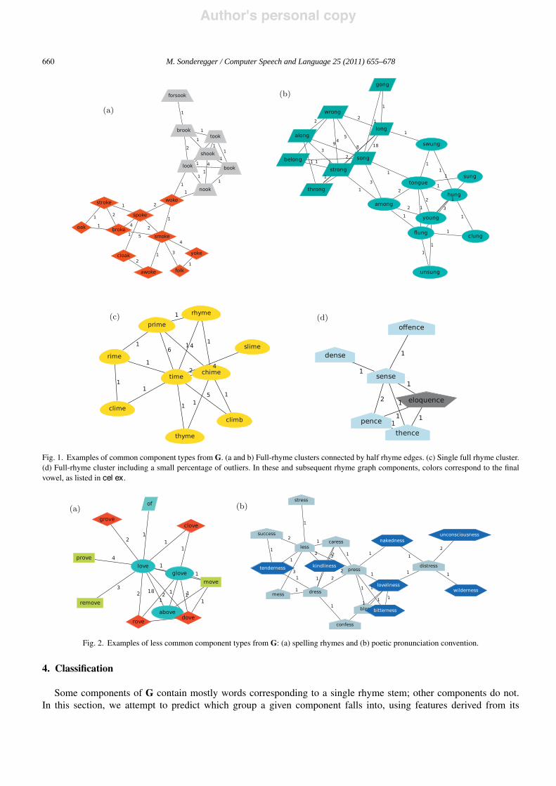
We denote the rhyme graph corresponding to the corpus as G. G has 70 connected components; we call this set C.To visualize the graphs corresponding to rhyme data, we use GraphViz, an open-source graph visualization package(AT&T Research, 2006; Gansner and North, 1999). In all graphs shown here, colors indicate pronunciations of finalsyllable vowels, a necessary but not sufficient condition for full rhyme (for both long and short rhyme stems); and the{wi, wj} edge is labeled with nij. Because the whole graph is too large to show, we illustrate what G looks like throughsome example components.

Common component types: Many components consist entirely (Fig. 1(c)) or mostly (Fig. 1(d)) of words with asingle rhyme stem. When components contain more than one rhyme stem, they often consist of two or more denseclusters largely corresponding to different rhyme stems, with relatively few edges between clusters. For example, thecomponents in Fig. 1(a) and (b) consist of two well-defined clusters, and Fig 5(c) shows a component with 10 clusters,discussed further below. These two types of components make up much of the graph, though some are not as cleanas the examples shown. In components made of several clusters, the clusters seem to correspond to words primarilysharing a single rhyme stem (and connected by full rhymes), with edges between these clusters corresponding to halfrhymes. This intuition is confirmed below (Sections 4 and 5) in the classification and partitioning tasks.

Less common component types: Two other types of components occur, though less frequently. Components such asFig. 2(a) contain many edges corresponding to half rhymes between words with similar spellings, or spelling rhymes(Wyld, 1923). Components such as Fig. 2(b) contain many edges which correspond to full rhymes if a special literarypronunciation is used for one word (usually ending in a suffix).10 For example, reading -ness as [n!s] would make allhalf rhymes in Fig. 2(b) full, and reading -ity as [itai] would make rhymes such as sanity:fly full (using short rhymestems). We call such cases poetic pronunciation conventions (PPCs). PPCs often (as in Fig. 2(b)) result in spellingrhymes, but not always (as in sanity:hi).

3.3. Summary

We have introduced rhyme graphs, the corpus, and its rhyme graph G. We found that most of its componentsconsist of one or more well-defined clusters, reflecting the real pronunciation of words, while the rest reflect poeticusage. We now make practical use of the relationship between structure and pronunciation seen in most components ofG.

10 In most cases, these pronunciations are “literary” in the sense that they have not been used in colloquial English for centuries (Wyld, 1936).



Fig. 1. Examples of common component types from G. (a and b) Full-rhyme clusters connected by half rhyme edges. (c) Single full rhyme cluster.(d) Full-rhyme cluster including a small percentage of outliers. In these and subsequent rhyme graph components, colors correspond to the finalvowel, as listed in cel ex.

Fig. 2. Examples of less common component types from G: (a) spelling rhymes and (b) poetic pronunciation convention.

4. Classification

Some components of G contain mostly words corresponding to a single rhyme stem; other components do not.In this section, we attempt to predict which group a given component falls into, using features derived from its



graph structure. We first describe the feature set and a binary classification task implementing the intuitive notion ofcomponent “goodness”, then train and evaluate several classifiers for this task over the components of G. We find thatthe “goodness” of a component – corresponding to whether it contains half-rhymes – can be largely determined fromgraph structure alone, independent of any information about pronunciation or spelling.

4.1. Feature set

Let G = (V, E, W) be a connected component of G, where W are the unnormalized weights (wij = nij), with n nodes(v1, . . . , vn), and m edges, corresponding to {vi,vj} pairs with wij > 0. Define nij, di, wij , d#

i , and ai as above (Section3.1). In addition, we need a matrix of distances, d, between nodes in a component. Because higher weight shouldcorrespond to smaller distance, we use

dij =�

1/wij if wij /= 0

' otherwise

We define 17 features describing the structure of G, of two types. Non-spectral features are properties of graphs(e.g. diameter, maximum clique size) often used in research on social networks (Wasserman and Faust, 1994; Scott,2000), and complex networks more generally (Newman, 2003; Bornholdt and Schuster, 2003). Spectral features arebased on the eigenvalues of the Laplacian of G, which are intimately related to G’s structure (Chung, 1997).11

4.1.1. Non-spectral featuresWe first define some non-spectral properties of graphs often used in network research.Let g be the matrix of geodesics using distances d: gij is the length of the shortest path between vertices i and j. The

vertex betweenness centrality of v % V is the percentage of geodesics that include v.Considering G as an unweighted graph (with {vi, vj} % E if wij > 0), the clustering coefficient of vi % V is the

number of edges between neighbors of v, divided by the total number possible:

C(vi) = |{vj, vk} % E : vi"vj"vk||{vj, vk} % E : vi"vj, vi"vk|

We define 10 non-spectral features:

• mean/max nzd degree: Mean/maximum of the ai, divided by n ( 1.• edge rat: (m/(n(n ( 1)/2)), the fraction of all possible edges present.• max clique size nzd: Fraction of vertices in the largest clique of G.• max vtx bcty: Maximum vertex betweenness centrality.• diameter: Maximum of the gij.• mean shortest path: Mean of the gij.• radius: The minimum eccentricity of a vertex, where eccentricity (vi) = maxvj % V gij .• ccoeff: Mean clustering coefficient for vertices in V.• log size: log (n)

In addition, log size is z-scored across components, and diameter is divided by its maximum value acrosscomponents. With these normalizations made, no non-spectral feature transparently depends on the absolute size of acomponent. This makes the non-spectral features more comparable to spectral features, which are intuitively relatedto the “shape” of a graph, not its size.

4.1.2. Spectral featuresWe outline the relationship between the eigenvalues of G and measures of how “cuttable” G is, then define features

based on this connection.

11 A larger feature set including 18 other non-spectral features was initially tried, but did not give better classification performance. The non-spectralfeatures used here are the most predictive features from the larger set.



Graph Laplacians: There are several ways to define the Laplacian of a graph, which in general yield “different butcomplementary information” about its structure (Chung and Lu, 2006). We use three versions here.

Let A be the adjacency matrix of component G. Let N and D# be the diagonal matrices with diagonal elements aiand d#

i , respectively. The unweighted, unnormalized Laplacian is

L00 = N ( A

The weighted, unnormalized Laplacian is

L10 = D# ( W

The weighted, normalized Laplacian is

L11 = D#(1/2L10D

#(1/2

However, it is defined, the Laplacian’s eigenvalue spectrum is closely related to many properties of the underlyinggraph (G); the study of this connection is spectral graph theory (Chung, 1997). Graph eigenvalues are essential becausethey figure in a variety of bounds on quantities of interest about the underlying graph, such as finding the “best” partition,which are often provably NP-hard to compute. Our spectral features are based on several such bounds.

It can be quickly checked that L00, L10 and L11 (a) are positive semi-definite, which implies their eigenvalues arereal and positive (b) have smallest eigenvalue 0. Let !00, !10, and !11 be the second-smallest eigenvalues. Let !#

00 bethe largest eigenvalue of L00, and denote µ00 = 2 !00

!00+!#00

.

These eigenvalues can be used to bound several measures of the “cuttability” of a graph. Let E(S, S) be the set ofedges between a subset S ) V and its complement, and define vol(S) =

�v % Sai. The Cheeger constant of G is

hG = minS)G

|E(S, S)|min(vol(S),vol(S))

(1)

Intuitively, the Cheeger constant corresponds to a bipartition of G which balances two conflicting goals: make the twopieces as equal in size as possible, and separated by as few edges as possible.12 It can be shown (Chung, 1997) that

!00

2* hG *

�1 ( (1 ( !00)2 (2)

For the weighted case, define E(S, S) to be the sum over weights of edges between S and S#, and let vol(S) =�

i % Sd#i .

The Cheeger constant is then defined as in (1). Lower (Mohar, 1997, p. 32) and upper (Friedland and Nabben, 2002,p. 10) bounds on hG using !10, analogous to the unweighted case in (2), are:

!10

2* hG *

�

1 (�

1 ( !10

"

�2

(3)

where " is the minimum weighted degree of a vertex (min d#i).

Similarly, hG can be bounded using !11:

!11

2* hG * 2

+!11 (4)

Finally, we consider a different measure of the geometry of G. For the unweighted version of G (adjacency matrixN), given a subset X ) V, define the vertex boundary "(X) to be the vertices not in X, but adjacent to a vertex in X. Thenfor any subset, the ratio between its “perimeter” and “area” can be bounded from below (Chung, 1997):

vol("X)vol(X)

& 1 ( (1 ( µ00)2

1 + (1 ( µ00)2 (5)

Intuitively, if the perimeter/area ratio can be lower-bounded for all X, as in a circle, there is no good cut of G.

12 The Cheeger constant is also called “conductance”.



Based on these relationships between a graph’s eigenvalues and its “cuttability”, we define 7 spectral featurescorresponding to the bounds in (2)–(5):

• cut lower bound 1: !002

• cut upper bound 1:�

1 ( (1 ( !00)2


• cut upper bound 2:

�1 (

�1 ( !10

"

�2


• cut upper bound 3: 2+

!11

• subset perim/area bound: 1((1(µ00)2

1+(1(µ00)2

4.2. Experiments

We now describe a binary classification task involving this feature set, as well as subsets of these features.

4.2.1. Binary classification taskFor both short and long rhyme stem data, we wish to classify components of the rhyme graph as “positive” (consisting

primarily of true rhymes) or “negative” (otherwise). As a measure of component goodness, we use the percentage ofvertices corresponding to the most common rhyme stem, denoted most frequent rhyme stem percentage (MFRP). Thepronunciation of rhyme stems was manually determined from cel ex, as discussed above (Section 2.2). Intuitively,if a component is thought of as made up of vertices of different colors corresponding to different rhyme stems, theMFRP is the percentage of vertices with the most common color.13 For example, the component in Fig. 1(b) has MFRP=52.9 (corresponding to [$!] rhyme stems). To turn this into a binary classification task, we choose a threshold value,threshMFRP, arbitrarily set to 0.85 in tests described here. We fix threshMFRP for purposes of exposition; below(Section 4.3), we consider the effect of varying threshMFRP on performance. We wish to separate components withMFRP<threshMFRP from components with MFRP>threshMFRP.

As a measure of how predictive different features are for classification, Table 4 shows the information gain associatedwith each feature, for long and short RS data (see, e.g. Russell and Norvig, 2002). In both cases, there is a clearasymmetry between spectral and non-spectral feature predictiveness: every spectral feature is more predictive than allnon-spectral features.

4.2.2. Feature setsGiven that we have a large number of features relative to the number of components to be classified, and that many

features are strongly correlated, we are in danger of overfitting if the full feature set is used. For each of long and shortRS data, we define two smaller feature sets.

The first is the subset given by correlation-based feature selection (CFS; Hall, 1999), a standard feature-selectionstrategy in which a subset is sought which balances features’ predictiveness with their relative redundancy. We used theimplementation of CFS in Weka (Witten and Frank, 2005), an open-source machine learning package. Table 4 showsthe optimal CFS subsets for long and short RS data.

The second subset used, for each of the short and long RS datasets, is simply the most predictive feature: cutlower bound 1 for short RS data, and subset perim/area bound for long RS data.

13 A node’s color in the rhyme graph components shown here corresponds to its final vowel nucleus, not its rhyme stem. However, within anindividual component, there is usually at most one rhyme stem with a given final vowel nucleus, so that each color can be thought of as representingone rhyme stem. We use colors to represent final vowels, rather than rhyme stems, because the number of different rhyme stems ("50) makes itimpractical to represent each one by a visually distinct color.



Table 4Information gain of features for short and long rhyme stem classification. (Dashed line divides spectral and non-spectral features.) Feature subsetsgiven by correlation-based feature selection are marked with asterisks. The maximally predictive features are cut lower bound 1 for shortRS data and subset perim/area bound for long RS data.

Short RS Info. gain Long RS Info. gain

cut upper bound 1* 0.57 subset perim/area bound* 0.54cut lower bound 1* 0.57 cut lower bound 2* 0.53subset perim/area bound* 0.54 cut lower bound 3* 0.50cut upper bound 3 0.49 cut upper bound 3 0.50cut lower bound 3* 0.49 cut lower bound 1* 0.46cut lower bound 2 0.45 cut upper bound 1 0.46cut upper bound 2 0.42 cut upper bound 2 0.38

max nzd degree 0.29 mean nzd degree 0.28mean nzd degree 0.26 edge rat 0.28edge rat 0.26 max vtx bcty* 0.24radius* 0.23 radius 0.23mean shortest path 0.22 mean shortest path 0.22max clique size nzd 0.22 diameter 0.21diameter 0.22 max clique size nzd 0.20log size 0.19 max nzd degree 0.19max vtx bcty* 0.18 log size 0.17ccoeff* 0.18 ccoeff* 0.15

Table 510-Fold cross-validated accuracies (percentage correct) and F-measures for several classifiers over components of G, for short (top) and long(bottom) rhyme stems. For each rhyme stem type, CFS subset and most predictive feature given in Table 4.

Accuracy F-measure

Base KNN-5 KNN-10 CART SVM Base KNN-5 KNN-10 CART SVM

Shor t All features 55.7 88.6 85.7 81.4 85.7 71.6 89.5 86.8 83.5 87.5CFS subset 55.7 87.4 85.7 81.4 88.6 71.6 88.6 87.2 83.5 90.2Most pred. feature 55.7 87.1 90.0 85.7 90.0 71.6 88.6 91.1 85.7 88.9

Long All features 47.1 85.7 84.3 85.7 81.4 47.1 84.8 82.5 85.3 80.0CFS subset 47.1 82.9 85.7 85.7 87.1 47.1 81.8 84.4 85.3 85.7Most pred. feature 47.1 85.7 84.3 88.6 84.3 47.1 85.3 83.1 88.6 82.0

4.2.3. ClassifiersThere are 33 positive/37 negative components for long rhyme stems, and 39 positive/31 negative components for

short rhyme stems. As a baseline classifier Base, we use the classifier which simply labels all components as positive.We use three non-trivial classifiers: k-nearest neighbors, classification and regression trees (Breiman et al., 1984)

and support vector machines (Vapnik, 1995). We used Weka’s versions of these classifiers, with the following settings:

• KNN-5 /KNN-10: Classify by 5/10 nearest neighbors, using Euclidean distance.• CART: Binary decision tree chosen using minimal cost-complexity pruning, with five-fold internal cross validation

(numFoldsPruning =5), minimum of 2 observations at terminal nodes.• SVM: Support vector machine trained using sequential minimal optimization (Platt, 1999). All features normalized,

C = 1 (complexity parameter), linear homogeneous kernel.

4.2.4. ResultsTable 5 shows classification results using 10-fold cross-validation, stratified by dataset (short vs. long RS), feature

set, and classifier. Classifiers’ performances are given as accuracies (percentage of instances correctly labeled) andF-measures (harmonic mean of precision and recall).



MFRP Threshold

Acc

urac

y

0.2

0.4

0.6

0.8

1.0Short RS

0.75 0.80 0.85 0.90 0.95 1.00

Long RS

0.75 0.80 0.85 0.90 0.95 1.00

ClassifierBase

KNN5KNN10CARTSVM

MFRP Threshold

F m

easu

re

0.4

0.5

0.6

0.7

0.8

0.9

1.0Short RS

0.75 0.80 0.85 0.90 0.95 1.00

Long RS

0.75 0.80 0.85 0.90 0.95 1.00

ClassifierBase

KNN5KNN10CART

SVM

Fig. 3. 10-Fold cross-validated accuracies and F-measures for several classifiers over components of G, for short and long rhyme stems, asthreshMFRP is varied; the component size cutoff is fixed at 6. Only the most predictive feature is used for classification.

Unsurprisingly, in all cases the non-trivial classifiers perform better than the baseline classifier. Performance usingeither feature subset is significantly better than for the full feature set, suggesting overfitting or badly predictivefeatures. Performance (using non-trivial classifiers) is better for short rhyme stems than for long rhyme stems, thoughthe difference is only statistically significant for F-measures.14 This could be taken to argue that the corpus’ rhymesare better described using short rhyme stems.

It is striking that across classifiers, performance measures, and rhyme stem types, performance using only onefeature (the most predictive feature) is not clearly worse than performance using a subset of features given by a featureselection procedure (CFS). For both long and short rhyme stems, the most predictive feature (and the first severalmost predictive features generally, as seen in Table 4) is spectral. Classifying components then comes down to a singlefeature which can be interpreted in terms of graph structure: more cuttable components (lower !) are classified asnegative, while less cuttable components (higher !) are classified as positive.

4.3. Sensitivity analysis

To construct the dataset used in the classification experiments, two free parameters were fixed: the threshold MFRP(threshMFRP), and the component size cutoff (CSC). Varying threshMFRP changes which components havepositive labels, while changing CSC changes the number of components in the dataset. We now briefly check howsensitive the experimental results summarized in Table 5 are to varying these parameters, to make sure that the particularvalues chosen are not responsible for the good performance of our classifiers. We re-ran all experiments for the mostpredictive feature condition, changing the dataset by varying one of threshMFRP and CSC at a time.15

Because the goal of the classification task is to distinguish components which correspond mostly to a single rhymestem from those which do not, only values of threshMFRP relatively near 1 make sense. (It would not make sense,for example, to define “good” components as those with MFRP>0.5.) We consider threshMFRP % [0.75, 1]. Fig. 3shows accuracies and F-measures for classification on data resulting from values of threshMFRP in this range, withCSC kept fixed at 6. For short rhyme stem experiments, accuracies for non-trivial classifiers range between 79 and95%, and F-measures range between 78 and 97%. For long rhyme stem experiments, accuracies range between 70 and92%, while F-measures range greatly, between 46 and 92%. For both short and long rhyme stems, for all classifiers,two points are important: no classifier achieves its best performance at threshMFRP =0.85, and there is a range ofvalues including threshMFRP =0.85 within which performance varies little.

14 p = 0.21 for accuracies, p = 0.01 for F-measures, Wilcoxson paired rank-sum test.15 Which feature was most predictive changed as threshMFRP and CSC were changed, but was always a spectral feature.



Component size cutoff

Acc

urac

y

0.3

0.4

0.5

0.6

0.7

0.8

0.9

1.0

Short RS

4 5 6 7 8 9 10

Long RS

4 5 6 7 8 9 10

ClassifierBase

KNN5KNN10CARTSVM

Component size cutoff

F m

easu

re

0.4

0.5

0.6

0.7

0.8

0.9

1.0

Short RS

4 5 6 7 8 9 10

Long RS

4 5 6 7 8 9 10

ClassifierBase

KNN5KNN10CARTSVM

Fig. 4. 10-Fold cross-validated accuracies and F-measures for several classifiers over components of G, for short and long rhyme stems, as thecomponent size cutoff is varied; threshMFRP is fixed at 0.85. Only the most predictive feature is used for classification.

As discussed above (Section 3.2), CSC must be at least 4 for spectral features to make sense for all components;we consider CSC % [4, 10]. Fig. 4 shows accuracies and F-measures for classification on data resulting from values ofCSC in this range, with threshMFRP kept fixed at 0.85. For short rhyme stem experiments, accuracies for non-trivialclassifiers range between 81 and 90%, and F-measures range between 77 and 92%. For long rhyme stem experiments,accuracies range between 61 and 90%, while F-measures range between 51 and 89%. The same two points hold as forthe threshMFRP case: no classifier achieves its best performance at CSC=6, and there is a range of values includingCSC=6 within which performance varies little.

Classification performance can change significantly as threshMFRP and CSC are varied, especially for experi-ments using long rhyme stems. However, performance is not optimal for the fixed values of threshMFRP and CSCused above, and for most experiments, the change in performance when these parameters are varied near their fixedvalues is small. We can thus conclude that the good performance obtained in Section 4.2 is not a result of the particularvalues used for threshMFRP and CSC.

4.4. Summary

We have found that spectral features are more predictive of component goodness than non-spectral features; andthat although different spectral features in principle provide independent information about components, classifiersusing a single spectral feature have 85–90% accuracy, significantly better than a baseline classifier, and in line withclassifiers trained on an optimized subset of features. We have also shown that this performance is not an artifact of theparticular values chosen for two free parameters used to construct the dataset. For both short and long rhyme stems,the single spectral feature corresponds to how “cuttable” each component is. We have thus confirmed the intuition thatby and large, the bad components are those for which a good partition exists. We now see whether such good partitionscan be used to increase the quality of the dataset itself.

5. Partitioning

For each connected component of G, we would like to find the best partition into several pieces. The optimal numberof pieces is not known beforehand, and if no good partition exists, we would like to leave C unpartitioned. This generalproblem, called graph partitioning or community detection, is the subject of much recent work (see Fortunato, 2010;Fortunato and Castellano, 2009 for reviews). In this section, we apply one popular approach, modularity maximization,to the connected components of G, resulting in a subgraph G# ) G. We show that by several measures for comparinggraph partitions in general and rhyme graphs in particular, G# represents “better” data than G, relative to the goldstandard of 1-1 correspondence between rhyme stems and components.



5.1. Modularity

Many community detection algorithms attempt to find a partition which maximizes a measure of partition quality.Intuitively, given a hypothesized partition of a graph into subsets, we measure how connected the vertices in each subsetare to each other (relative to the rest of the graph), versus how connected we would expect them to be by chance givenno community structure, and sum over subsets. The most commonly used formalization of this idea is modularity, ameasure introduced by Newman and Girvan (2004).

Consider a partitionP of a graph G = (V, E) (unweighted) with n vertices, m edges, and adjacency matrix A. Considera random graph G# = (V, E#), in which there are m edges, vertices have the same degrees {ai} as in E, and the probabilityof an edge being placed between i and j is proportional to aiaj. The difference between the observed and expectednumber of edges between i and j is then

Aij

m( aiaj

2m2

This quantity is summed over all pairs of vertexes belonging to the same community:

Q(G,P) =�

{i,j}

�Aij

m( aiaj

2m2

�"(Pi, Pj) (6)

where Pi and Pj are the communities of vertices i and j, and " is the Kronecker delta. Q(G,P) is called the modularityof G under partition P.

In the weighted case, given G = (V, E, W) and partition P, let di =�

i"jwij and m# =�

{i,j}wij . By analogy to (6),modularity is defined as

Q(G,P) =�

{i,j}

�wij

m# ( didj

2m#2

�"(Pi, Pj) (7)

5.2. Modularity maximization

Given the weighted graph G corresponding to a connected component of a rhyme graph, we would like to find thepartition P! which maximizes modularity: P! = argmaxPQ(G,P). Let Q! , Q(G,P!). Because the trivial partition(where P = {G}) has modularity 0, Q! & 0. It can be shown that modularity is always less than 1 (Fortunato, 2010).Thus, Q! % [0, 1].

An exhaustive search forP! intuitively seems hard due to the exponential growth of possible partitions to be checked,and is in fact NP-complete (Brandes et al., 2007). However, in practice very good approximation algorithms exist forgraphs of the size considered here (Fortunato and Castellano, 2009). Such algorithms find a partition P approximatingP!, which increases modularity by #Q. Because the trivial partition has modularity 0 and Q! * 1:

0 * #Q * Q! * 1 (8)

The algorithm used here is a variant of simulated annealing (SA), adapted for modularity maximization by Meduset al. (2005). Here modularity acts as the “energy” (with the difference that modularity is being maximized, whileenergy is usually minimized), graph vertices are “particles”, transferring a vertex from one subset to another is a“transition”, and the state space is the set of possible partitions. In addition, every state (partition) includes exactlyone empty subset. This does not change a given partition’s modularity (since no terms for the empty subset arepart of the sum in Eq. (7)), but allows for transitions where a new subset (of one vertex) is created. (Whenever avertex is transferred to the empty subset from a subset with at least 2 vertices, so that no empty subset remains, anew empty subset is added to the partition.) Our implementation of SA (in Matlab) is described in pseudocode inAlgorithm 1.



Algorithm 1. Find a partition of P : V - N of G which maximizes modularity (Eq. (7)), using simulated annealing.Input: Weighted, connected G = (V,E,W )β ∈ (0, 1)α > 1thresh, maxsteps, reps∈

Qmax ← 0Smax ← {V }for i = 1 . . . reps do

S ← random initial partition of V consisting of between 2 and n− 1 subsets.Add an empty subset to S.Q← Q(W, S ) ### from Eqn. 7t← 0, lastaccept ← 0while (t −lastaccept) < thresh and t < maxsteps dot← t + 1Choose random v ∈ V .s(v)← subset of S containing v.Choose subset σ ∈ S ∩s(v).S� ← S with v moved from s(v) to σ. ### proposed transition S → S�

Q� ← Q(W, S �)if Q� > Qmax then

Qmax ← Q� ### Keep track of maximum Q partition seenSmax ← S�

end ifq ← min{1, e−β(Q−Q�)}.With probability q, accept. ### MCMC stepif accept then

S ← S�

Q← Q�

lastaccept←tIf S contains no empty subset, add one.

end ifβ ← αβ ### lower pseudo-temperature

end whileend forreturn P corresponding to Smax.

5.3. Experiment

LetC be the connected components of G, with wij equal to the number of times the rhyme {vi, vj} occurs in the corpus.For each component Ci % C, we found a partition Pi = {Ci

1, . . . , Cini

} maximizing Q by running Algorithm 1 thirtytimes, with $ = 0.01, % = 1.01, lastaccept =10000, and maxsteps =200000. Removing all edges between verticesin Ci

j and Cik (.i; j, k * ni, j /= k) induces a subgraph G# ) G, with connected components C# =

�iPi. Figs. 5 and 6

show examples of partitions found for some components of G, discussed further below.

5.3.1. ResultsThe algorithm was successful at increasing modularity by partitioning components of G, perhaps overmuch: for

every component Ci % C, a partition with higher modularity (Q > 0) than the trivial partition (Q = 0) was found. As aresult, there are |C#| = 257 components in G#, compared with |C| = 70 in G. Our concern here is the extent to whichthese increases in modularity improve the quality of the rhyme graph. We take the “gold standard” to be a graph wherethere is a 1-1 correspondence between rhyme stems and components.

Does partitioning bring the rhyme graph closer to this gold standard? We first show some examples of the partitionsfound for individual components of G, then discuss some quantitative measures of how the quality (made more precisebelow) of G# compares to that of G.

5.4. Examples

For many components, partitioning by modularity maximization yields the desired result: a component includingseveral rhyme stems is broken up into smaller components, each corresponding to a single rhyme stem. We give twoexamples.



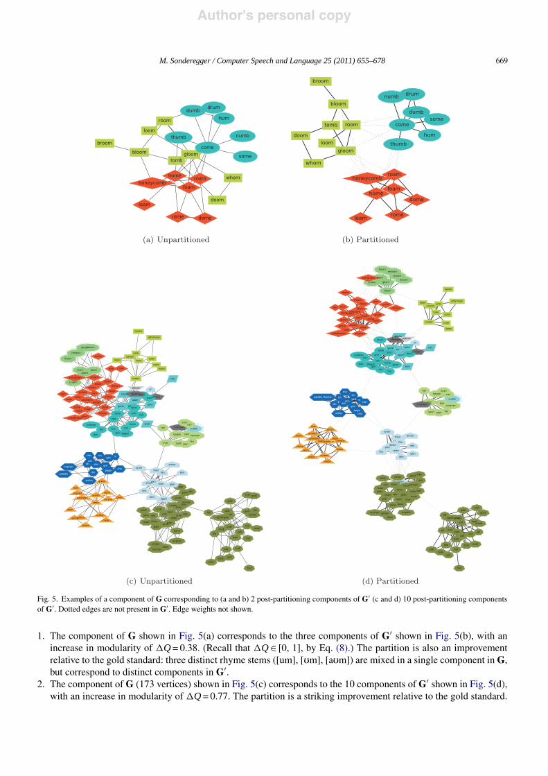
Fig. 5. Examples of a component of G corresponding to (a and b) 2 post-partitioning components of G# (c and d) 10 post-partitioning componentsof G#. Dotted edges are not present in G#. Edge weights not shown.

1. The component of G shown in Fig. 5(a) corresponds to the three components of G# shown in Fig. 5(b), with anincrease in modularity of #Q = 0.38. (Recall that #Q % [0, 1], by Eq. (8).) The partition is also an improvementrelative to the gold standard: three distinct rhyme stems ([um], [$m], [a$m]) are mixed in a single component in G,but correspond to distinct components in G#.

2. The component of G (173 vertices) shown in Fig. 5(c) corresponds to the 10 components of G# shown in Fig. 5(d),with an increase in modularity of #Q = 0.77. The partition is a striking improvement relative to the gold standard.



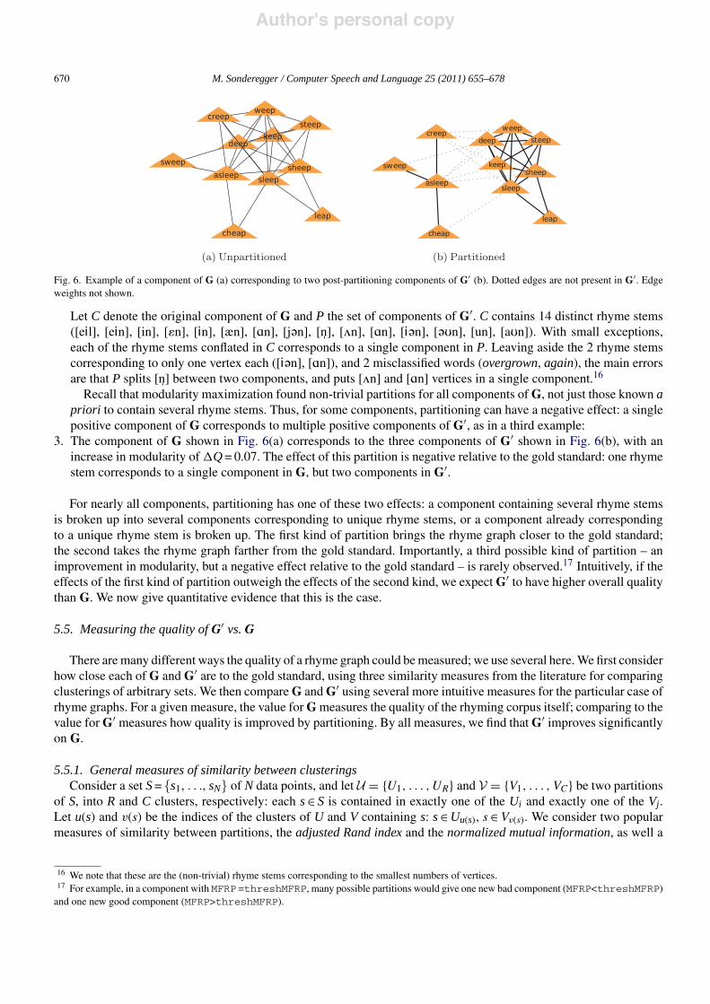
Fig. 6. Example of a component of G (a) corresponding to two post-partitioning components of G# (b). Dotted edges are not present in G#. Edgeweights not shown.

Let C denote the original component of G and P the set of components of G#. C contains 14 distinct rhyme stems([eil], [ein], [in], [!n], [in], [æn], [%n], [j#n], [ &n], ['n], [%n], [i#n], [#$n], [un], [a$n]). With small exceptions,each of the rhyme stems conflated in C corresponds to a single component in P. Leaving aside the 2 rhyme stemscorresponding to only one vertex each ([i#n], [%n]), and 2 misclassified words (overgrown, again), the main errorsare that P splits [ &n] between two components, and puts ['n] and [%n] vertices in a single component.16

Recall that modularity maximization found non-trivial partitions for all components of G, not just those known apriori to contain several rhyme stems. Thus, for some components, partitioning can have a negative effect: a singlepositive component of G corresponds to multiple positive components of G#, as in a third example:

3. The component of G shown in Fig. 6(a) corresponds to the three components of G# shown in Fig. 6(b), with anincrease in modularity of #Q = 0.07. The effect of this partition is negative relative to the gold standard: one rhymestem corresponds to a single component in G, but two components in G#.

For nearly all components, partitioning has one of these two effects: a component containing several rhyme stemsis broken up into several components corresponding to unique rhyme stems, or a component already correspondingto a unique rhyme stem is broken up. The first kind of partition brings the rhyme graph closer to the gold standard;the second takes the rhyme graph farther from the gold standard. Importantly, a third possible kind of partition – animprovement in modularity, but a negative effect relative to the gold standard – is rarely observed.17 Intuitively, if theeffects of the first kind of partition outweigh the effects of the second kind, we expect G# to have higher overall qualitythan G. We now give quantitative evidence that this is the case.

5.5. Measuring the quality of G# vs. G

There are many different ways the quality of a rhyme graph could be measured; we use several here. We first considerhow close each of G and G# are to the gold standard, using three similarity measures from the literature for comparingclusterings of arbitrary sets. We then compare G and G# using several more intuitive measures for the particular case ofrhyme graphs. For a given measure, the value for G measures the quality of the rhyming corpus itself; comparing to thevalue for G# measures how quality is improved by partitioning. By all measures, we find that G# improves significantlyon G.

5.5.1. General measures of similarity between clusteringsConsider a set S = {s1, . . ., sN} of N data points, and let U = {U1, . . . , UR} and V = {V1, . . . , VC} be two partitions

of S, into R and C clusters, respectively: each s % S is contained in exactly one of the Ui and exactly one of the Vj.Let u(s) and v(s) be the indices of the clusters of U and V containing s: s % Uu(s), s % Vv(s). We consider two popularmeasures of similarity between partitions, the adjusted Rand index and the normalized mutual information, as well a

16 We note that these are the (non-trivial) rhyme stems corresponding to the smallest numbers of vertices.17 For example, in a component with MFRP =threshMFRP, many possible partitions would give one new bad component (MFRP<threshMFRP)

and one new good component (MFRP>threshMFRP).



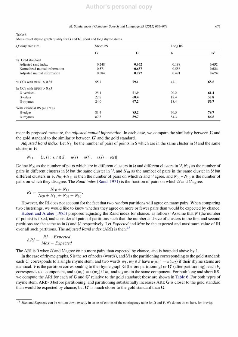
Table 6Measures of rhyme graph quality for G and G#, short and long rhyme stems.

Quality measure Short RS Long RS

G G# G G#

vs. Gold standardAdjusted rand index 0.248 0.662 0.188 0.652Normalized mutual information 0.571 0.637 0.556 0.634Adjusted mutual information 0.584 0.777 0.491 0.674

% CCs with MFRP > 0.85 55.7 79.1 47.1 68.5

In CCs with MFRP > 0.85% vertices 25.1 71.9 20.2 61.4% edges 22.8 68.4 18.4 57.8% rhymes 24.0 67.2 18.4 53.7

With identical RS (all CCs)% edges 81.4 85.2 76.3 79.7% rhymes 87.3 89.7 84.3 86.5

recently proposed measure, the adjusted mutual information. In each case, we compare the similarity between G andthe gold standard to the similarity between G# and the gold standard.

Adjusted Rand index: Let N11 be the number of pairs of points in S which are in the same cluster in U and the samecluster in V:

N11 = |{s, t} : s, t % S, u(s) = u(t), v(s) = v(t)|

Define N00 as the number of pairs which are in different clusters in U and different clusters in V, N01 as the number ofpairs in different clusters in U but the same cluster in V, and N10 as the number of pairs in the same cluster in U butdifferent clusters in V. N00 + N11 is then the number of pairs on which U and V agree, and N01 + N10 is the number ofpairs on which they disagree. The Rand index (Rand, 1971) is the fraction of pairs on which U and V agree:

RI = N00 + N11

N00 + N11 + N01 + N10.

However, the RI does not account for the fact that two random partitions will agree on many pairs. When comparingtwo clusterings, we would like to know whether they agree on more or fewer pairs than would be expected by chance.

Hubert and Arabie (1985) proposed adjusting the Rand index for chance, as follows. Assume that N (the numberof points) is fixed, and consider all pairs of partitions such that the number and size of clusters in the first and secondpartitions are the same as in U and V, respectively. Let Expected and Max be the expected and maximum value of RIover all such partitions. The adjusted Rand index (ARI) is then:18

ARI = RI ( Expected

Max ( Expected

The ARI is 0 when U and V agree on no more pairs than expected by chance, and is bounded above by 1.In the case of rhyme graphs, S is the set of nodes (words), andU is the partitioning corresponding to the gold standard:

each Ui corresponds to a single rhyme stem, and two words w1, w2 % S have u(w1) = u(w2) if their rhyme stems areidentical. V is the partition corresponding to the rhyme graph G (before partitioning) or G# (after partitioning): each Vjcorresponds to a component, and v(w1) = v(w2) if w1 and w2 are in the same component. For both long and short RS,we compute the ARI for each of G and G# relative to the gold standard; these are shown in Table 6. For both types ofrhyme stem, ARI> 0 before partitioning, and partitioning substantially increases ARI: G is closer to the gold standardthan would be expected by chance, but G# is much closer to the gold standard than G.

18 Max and Expected can be written down exactly in terms of entries of the contingency table for U and V. We do not do so here, for brevity.



Normalized mutual information, adjusted mutual information: To define the mutual information of two partitionsof a set, we must first state them in terms of random variables. Let P(i) denote the probability that a point s % S hasu(s) = i, P#(j) the probability that v(s) = j, and P##(i, j) the probability that u(s) = i and v(s) = j:

P(i) = |Ui|N

, P #(j) = |Vj|N

, P ##(i, j) = |Ui / Vj|N

The entropy and mutual information (MI) of partitions U and V are then defined via these random variables:

H(U) = (R�

i=1

P(i) log P(i), H(V) = (S�

j=1

P #(j) log P #(j), I(U,V) =R�

i=1

S�

j=1

P ##(i, j) log�

P ##(i, j)P(i)P #(j)

�

MI is a symmetric measure of how predictive two random variables are of each other. In the case of clustering, MIquantifies how similarly two partitions cluster the same set of data points. MI is non-negative, and is upper bounded bymin{H(U), H(V)}. Based on these observations, Strehl and Ghosh (2003) proposed the normalized mutual information(NMI) as a measure for comparing partitions:

NMI(U,V) = I(U,V)+H(U)H(V)

NMI is bounded by 0 and 1. Unlike ARI, NMI is not adjusted for chance. A version of MI adjusted for chance, theadjusted mutual information (AMI), has recently been proposed by Vinh et al. (2009). Adjustment for chance is donesimilarly as for ARI, and we do not give details here. Like ARI, AMI is bounded above by 1, and is 0 when U and Vagree on no more pairs than expected by chance.

For our case of rhyme graphs, we consider both NMI and AMI. U and V are defined as above (for ARI). For bothlong and short rhyme stems, we compare G and G# by computing NMI and AMI for each, relative to the gold standard;these are shown in Table 6. For both types of rhyme stem, partitioning increases NMI. AMI shows similar patternsto ARI: G is closer to the gold standard than would be expected by chance, but G# is significantly closer to the goldstandard than G.

5.5.2. Intuitive measures of rhyme graph qualityThe general similarity measures just considered tell us that G# is closer to the gold standard than G, but not how it

is closer. To better understand how G compares with G#, we consider several more intuitive measures of quality forthe case of rhyme graphs.

Component MFRP: Recall that above (Section 4.2), we divided components of G into positive and negative classes,based on whether MFRP was above or below a threshold value. One measure of a graph’s quality is how large thepositive class is: the percentage of components with MFRP>threshMFRP. If we wish to weight components by theirsizes, we could consider the percentage of vertices, edges (adjacent vertices) or rhymes (weights on adjacent vertices)lying in components with MFRP>threshMFRP.

Rows 4–7 of Table 6 give these four measures for G and G#, for short and long rhyme stems. G# improves substantially(21–46%) on G in each case. Although G had low scores to begin with, the dramatic increases seen confirm theintuition that partitioning was largely successful in decreasing the number of components, especially large components,containing several rhyme stems.

For a more direct look at the effect of partitioning on MFRP, we can consider how its distribution (across allcomponents) changed from G to G#. Fig. 7 shows histograms of MFRP for components of G and G#, for short and longrhyme stems. It is visually clear that the distributions for G# (partitioned) are much more concentrated near 1 (samerhyme stem for all vertices of a component) than the distributions for G (unpartitioned). In particular, components withMFRP<0.5, like the example discussed above in Fig. 5(c), are almost completely gone.

Percentage identical rhyme stems: Instead of measuring the size of positive components in G and G#, we couldconsider a more basic quantity, without reference to components: the type and token percentage of full rhymes. Rows8–9 of Table 6 show the percentage of edges between vertices with identical rhyme stems, and the analogous percentageof rhymes (again for G, G#, and short and long rhyme stems). G# again improves on G in all cases. Although the gainsare much more modest (2–4%) than for whole components (above), they are important; they indicate that partitioningremoved many more edges corresponding to half rhymes than corresponding to full rhymes, supporting the intuition



Unpartitioned

MFRP

Num

ber

of c

ompo

nent

s05

101520253035

05

101520253035

0.2 0.4 0.6 0.8 1.0

Short R

SLong R

S

Partitioned

MFRP

Num

ber

of c

ompo

nent

s

0

50

100

150

0

50

100

150

0.2 0.4 0.6 0.8 1.0

Short R

SLong R

S

Fig. 7. Histogram of most frequent rhyme percentage (MFRP) for components of the unpartitioned (left) and partitioned (right) graphs, for short(top) and long (bottom) rhyme stems.

that many components of G are made up of “good” (mostly full rhymes) pieces connected by “bad” (half-rhyme)edges.

Component cuttability: In the classification task above, when the type of rhyme stem was fixed, we found that thedistinction between positive and negative components could be boiled down to a single spectral feature, representingthe quality of the best bipartition of a component: its “cuttability”. For short rhyme stems, this feature was cut lowerbound 1; for long rhyme stems it was subset perim/area bound. As a measure of how the cuttability ofcomponents was changed by partitioning, we can look at the distribution of these features (across components) for Gand G#, shown as histograms in Figs. 8 and 9.

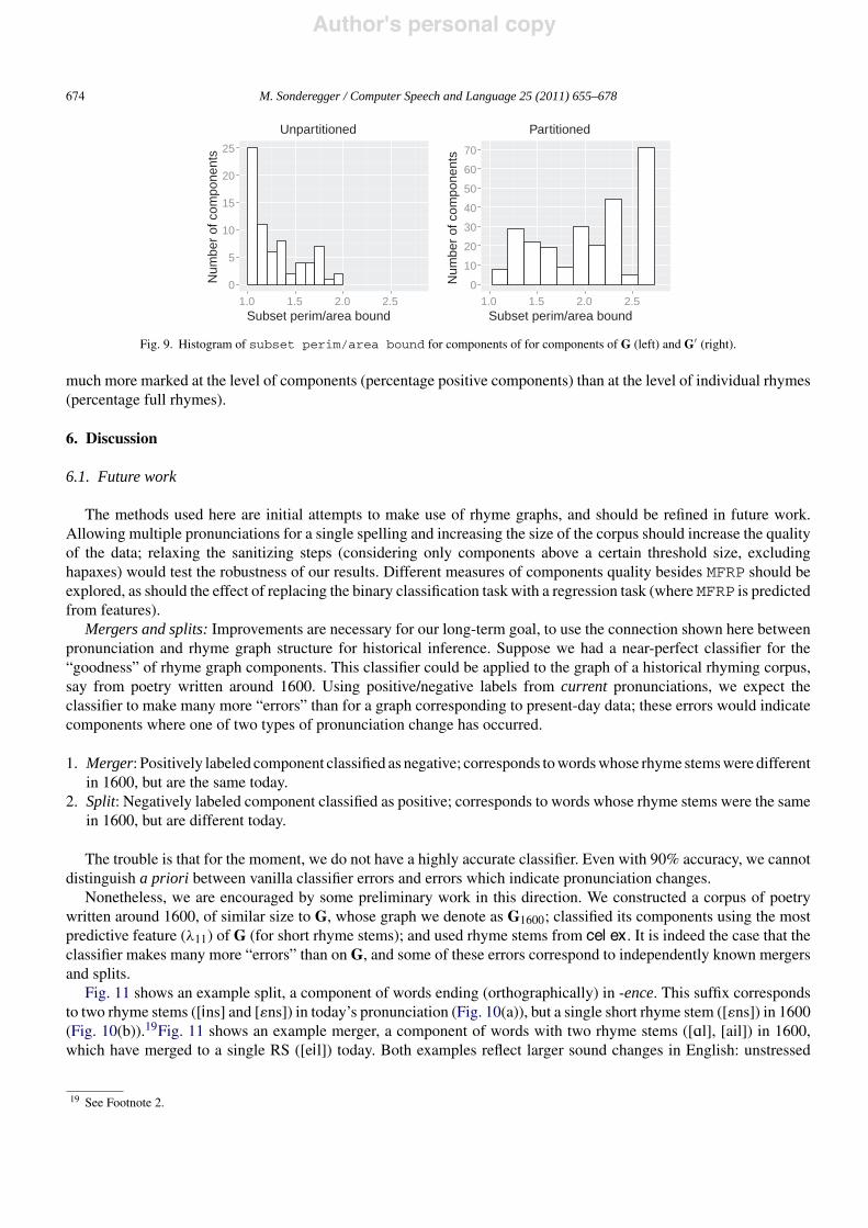
Recall that lower !11 and higher subset perim/area bound correspond to higher cuttability. !11 has mean0.22 for components of G and mean 0.93 for components of G#; further, the distribution of !11 is much less concentratednear 0 in G# than in G. subset perim/area bound has mean 1.23 for components of G and mean 2.06 for com-ponents of G#; also, its distribution is skewed right for G (skewness=0.84) and skewed left for G# (skewness = (0.18).Overall, the distributions of !11 and subset perim/area bound for G# versus G reflect that components of G#

are much less cuttable.

5.6. Summary

After partitioning G via modularity maximization to give G#, we found that by several measures, G# is closer than Gto the gold standard, where there is a 1-1 correspondence between rhyme stems and components. This improvement is

Unpartitioned

Cut lower bound 3 (!11)

Num

ber

of c

ompo

nent

s

0

5

10

15

20

25

0.0 0.5 1.0 1.5 2.0

Partitioned

Cut lower bound 3 (!11)

Num

ber

of c

ompo

nent

s

0

10

20

30

40

50

0.0 0.5 1.0 1.5 2.0

Fig. 8. Histogram of cut lower bound 3 (!11) for components of G (left) and G# (right).



Unpartitioned

Subset perim/area bound

Num

ber

of c

ompo

nent

s

0

5

10

15

20

25

1.0 1.5 2.0 2.5

Partitioned

Subset perim/area bound

Num

ber

of c

ompo

nent

s

0

10

20

30

40

50

60

70

1.0 1.5 2.0 2.5

Fig. 9. Histogram of subset perim/area bound for components of for components of G (left) and G# (right).

much more marked at the level of components (percentage positive components) than at the level of individual rhymes(percentage full rhymes).

6. Discussion

6.1. Future work

The methods used here are initial attempts to make use of rhyme graphs, and should be refined in future work.Allowing multiple pronunciations for a single spelling and increasing the size of the corpus should increase the qualityof the data; relaxing the sanitizing steps (considering only components above a certain threshold size, excludinghapaxes) would test the robustness of our results. Different measures of components quality besides MFRP should beexplored, as should the effect of replacing the binary classification task with a regression task (where MFRP is predictedfrom features).

Mergers and splits: Improvements are necessary for our long-term goal, to use the connection shown here betweenpronunciation and rhyme graph structure for historical inference. Suppose we had a near-perfect classifier for the“goodness” of rhyme graph components. This classifier could be applied to the graph of a historical rhyming corpus,say from poetry written around 1600. Using positive/negative labels from current pronunciations, we expect theclassifier to make many more “errors” than for a graph corresponding to present-day data; these errors would indicatecomponents where one of two types of pronunciation change has occurred.

1. Merger: Positively labeled component classified as negative; corresponds to words whose rhyme stems were differentin 1600, but are the same today.

2. Split: Negatively labeled component classified as positive; corresponds to words whose rhyme stems were the samein 1600, but are different today.

The trouble is that for the moment, we do not have a highly accurate classifier. Even with 90% accuracy, we cannotdistinguish a priori between vanilla classifier errors and errors which indicate pronunciation changes.

Nonetheless, we are encouraged by some preliminary work in this direction. We constructed a corpus of poetrywritten around 1600, of similar size to G, whose graph we denote as G1600; classified its components using the mostpredictive feature (!11) of G (for short rhyme stems); and used rhyme stems from cel ex. It is indeed the case that theclassifier makes many more “errors” than on G, and some of these errors correspond to independently known mergersand splits.

Fig. 11 shows an example split, a component of words ending (orthographically) in -ence. This suffix correspondsto two rhyme stems ([ins] and [!ns]) in today’s pronunciation (Fig. 10(a)), but a single short rhyme stem ([!ns]) in 1600(Fig. 10(b)).19Fig. 11 shows an example merger, a component of words with two rhyme stems ([%l], [ail]) in 1600,which have merged to a single RS ([eil]) today. Both examples reflect larger sound changes in English: unstressed

19 See Footnote 2.



Fig. 10. Example of a “merger”: a component from G1600 classified (using short rhyme stems) as negative (!11 < 0.12), with MFRP>mfrpThreshaccording to modern pronunciation (a) but MFRP<mfrpThresh according to 1600 pronunciations (b). Edge weights not shown.

vowels have often reduced (to [#] or [i]) word-finally, and the vowels pronounced in Early Modern English as [%] and[ai] merged to [ei] by 1800 (Lass, 1992).

Other languages and poetic traditions: All methods used in this paper would be straightforward to extend to rhymingcorpora from other languages, provided that a pronunciation dictionary exists, and that the definition of the rhyme stemis changed appropriately. Indeed, it is important to check in future work whether the salient aspects of the Englishrhyme graphs considered here hold for other languages. If rhyme graphs do not show some sort of similar structurecross-linguistically, they cannot be used for pronunciation reconstruction in the most interesting cases, where thehistorical pronunciation of a language is unknown.

The methods used in this paper are also applicable to data from other poetic traditions. Rhyming in modern Englishpoetry requires that pairs of words be similar in a particular way near their endings. Different poetic traditions requirethat sets of words be similar, but define similarity very differently. In alliterative verse, pairs of words must begin withthe same phonemes; this is the dominant structuring device in most verse written in Old English (such as Beowulf) andOld Norse (the ancestor of modern-day Icelandic) (Godden and Lapidge, 1991; Ross, 2005). In Welsh poetry, differenttypes of cynghanedd (“harmony”) require various complex patterns of consonantal correspondence and rhyming amongwords within individual lines (Williams, 1952; Turco, 2000). In principle, the methods used in this paper could be

Fig. 11. Example of a “split”: a component from G1600 classified (using short rhyme stems) as positive (!11 > 0.12), with MFRP<mfrpThreshaccording to modern pronunciation (a) but MFRP>mfrpThresh according to 1600 pronunciations (b). Edge weights not shown.



extended to data from any poetic tradition, like alliterative verse or cynghanedd, where some sort of similarity betweenthe pronunciation of sets of words is implied by poetic form.

Full rhyme to half rhyme ratio For the poetic corpus considered here – English rhyming verse written around1900 – we found that the rhyme graph largely consists of full-rhyming clusters, connected by half-rhyming edges.A natural extension would be to check how robust this finding is for rhyming corpora where the ratio of halfrhymes to full rhymes is greater. In general, verse from various genres and dates will differ in how common halfrhymes are relative to full rhymes. For example, half rhymes seem to be more frequent in (contemporary, English-language) song lyrics than in rhyming poetry: in Katz’ (2008) English hip-hop corpus, 56% of rhymes have identicallong rhyme stems, compared to 84% in our corpus. Half rhymes also may be more common in translations ofrhyming verse into English, where faithfulness to the rhyme scheme may require that the translator use more halfrhymes.

6.2. Summary

In Sections 2 and 3, we introduced a corpus of rhymes from recent poetry, and explored its rhyme graph,G. We found most components of G either consist of a densely connected set of vertices (with edges corre-sponding to full rhymes), or several such sets, with few edges between sets (corresponding to half rhymes);relatively few components correspond to spelling rhymes or poetic pronunciation conventions. In other words,graph structure for the most part transparently reflects actual pronunciation. This is not a trivial fact: it couldhave been the case that half rhymes occur frequently enough to obscure the distinction between half and fullrhymes, or that spelling rhymes or poetic pronunciation conventions are widespread. That structure reflects pro-nunciation in poetry means it is (in principle) possible to “read off” pronunciation from structure, as discussedabove.

In Section 4, we found that spectral features are much more predictive of component “goodness” thannon-spectral features. Though it possible that a different set of non-spectral features would perform better,it is striking that for both short and long rhyme stems, no non-spectral feature is more predictive than anyspectral feature. We tentatively conclude that a component’s eigenvalue spectrum is more predictive of its“goodness” (i.e. class label) than the non-spectral measures often used in network research. Overall, we con-firmed the intuition that component goodness corresponds, for the most part, to whether a good partitionexists.

In Section 5, we found that applying modularity-based partitioning to components of G, resulting in a new graphG#, significantly improves the quality of the data, especially when seen from the perspective of components, rather thanindividual rhymes. For the short RS case, for example, 79% of components in G# are positive, corresponding to 72% ofwords, compared to 56%/25% for G. For the long-term goal of using rhyme graphs for pronunciation reconstruction,this is our most important finding: by partitioning components, we go from 50/50 positive/negative components to80/20. Where a random component of G contains many half rhymes at chance, a random component of G# probablydoes not.

Overall, we have shown three cases where it is possible and profitable to understand groups of rhymes in terms oftheir corresponding rhyme graphs. We can roughly summarize our findings by three correspondences between a givengroup of rhymes R, corresponding to a connected component G(R) of rhyme graph G:

Group of rhymes Component of rhyme graph

Most rhymes in R are full, fewer are half. 0 G(R) has community structure.R contains half-rhymes. 0 G(R) has a good partition.Which groups of rhymes in R are definitely full? 0 What is the best partition of G(R)?

We thus add to the recent body of work illustrating that in very different settings (e.g. Luce and Pisoni, 1998; Ferreri Cancho and Sole, 2001; Sigman and Cecchi, 2002; Steyvers and Tenenbaum, 2005; Mukherjee et al., 2008; Vitevitch,2008; Mukherjee et al., 2009a; Arbesman et al., 2010; Ferrer i Cancho, 2010 gives a bibliography), consideringlinguistic data as graphs (or networks) gives new insights into how language is structured and used. Specifically, like(Ferrer i Cancho et al., 2007; Biemann et al., 2009; Mukherjee et al., 2009b), we found a strong and striking associationbetween graph spectra and linguistic properties.



Acknowledgments

We thank Max Bane, Joshua Grochow, Ross Girshick, Partha Niyogi, Sravana Reddy, and Alan Yu for insightfuldiscussion and suggestions, as well as three anonymous reviewers for helpful comments. This work was supported inpart by a Department of Education GAANN Fellowship.

References

Arbesman, S., Strogatz, S., Vitevitch, M., 2010. The structure of phonological networks across multiple languages. Int. J. Bifurc. Chaos 20 (3),679–685.

AT&T Research, 2006. Graphviz (program), version 2.20.2. URL http://www.graphviz.org.Baayen, R., Piepenbrock, R., Gulikers, L.,1996. CELEX2, Linguistic Data Consortium, Philadelphia.Biemann, C., Choudhury, M., Mukherjee, A., 2009. Syntax is from Mars while Semantics from Venus! Insights from Spectral Analysis of

Distributional Similarity Networks. In: Proc. ACL-IJCNLP 2009 Conf., Association for Computational Linguistics, pp. 245–248.Bornholdt, S., Schuster, H. (Eds.), 2003. Handbook of Graphs and Networks: From the Genome to the Internet. Wiley-VCH, Weinheim.Brandes, U., Delling, D., Gaertler, M., Gorke, R., Hoefer, M., Nikoloski, Z., Wagner, D., 2007. On finding graph clusterings with maximum

modularity. In: Proc. 33rd Intl. Workshop Graph-Theor. Concepts Comput. Sci. (WG’07), Vol. 4769 of Lecture Notes in Computer Science,Springer, New York, pp. 121–132.

Breiman, L., Friedman, J., Olshen, R., Stone, C., 1984. Classification and Regression Trees. Wadsworth, Belmont, CA.Brooke, R., (Text from Project Gutenberg) 1915. The Collected Poems of Rupert Brooke.Chadwyck-Healey. Twentieth Century English Poetry. URL http://collections.chadwyck.co.uk/home/home20ep.jsp.Chesterton, G., (Text from Project Gutenberg) 1911. The Ballad of the White Horse.Chung, F., Lu, L., 2006. Complex graphs and networks. In: No. 107 in CBMS Regional Conf. Ser. Math, American Mathematical Society, Providence,

RI.Chung, F., 1997. Spectral graph theory. In: No. 92 in CBMS Regional Conf. Ser. Math, American Mathematical Society, Providence, RI.Crosland, T., (Text from Chadwyck-Healey Twentieth Century English Poetry (electronic resource)) 1917. The Collected Poems.Danielsson, B., 1955–1963. John Hart’s works on English orthography and pronunciation, 1551, 1569, 1570, no. 11 in Acta Universitatis Stock-

holmiensis. Stockholm Stud. in English.Danielsson, B., Gabrielson, A., 1972. Logonomia anglica (1619), no. 26–27 in Acta Universitatis Stockholmiensis. Stockholm Stud. in English.de la Mare, W., (Text from Project Gutenberg) 1901–1918. Collected Poems.Dobson, E., 1968. English Pronunciation 1500–1700, 2 volumes, 2nd ed. Clarendon, Oxford.Ferrer i Cancho, R., Sole, R., 2001. The small world of human language. Proc. Roy. Soc. Lond. Ser. B 268, 2261–2265.Ferrer i Cancho, R., Capocci, A., Caldarelli, G., 2007. Spectral methods cluster words of the same class in a syntactic dependency network. Int. J.

Bifurc. Chaos 17 (7), 2453–2463.Ferrer i Cancho, R., 2010. Bibliography on linguistic and cognitive networks [online]. Bibliography of applications of complex network theory and

graph theory to linguistic and cognitive networks (cited March 1, 2010).Fortunato, S., Castellano, C., 2009. Community structure in graphs. In: Meyers, R.A. (Ed.), Encyclopedia of Complexity and Systems Science.

Springer, New York, pp. 1141–1163.Fortunato, S., 2010. Community detection in graphs. Phys. Rep. 486, 75–174.Friedland, S., Nabben, R., 2002. On Cheeger-type inequalities for weighted graphs. J. Graph Theory 41 (1), 1–17.Gansner, E.R., North, S.C., 1999. An open graph visualization system and its applications to software engineering. Softw. Pract. Experience 30,

1203–1233.Georgian Poetry, volumes 1–4, 1911–1919 (Text from Project Gutenberg).Godden, M., Lapidge, M. (Eds.), 1991. The Cambridge companion to Old English literature. Cambridge University Press, Cambridge.Hall, M.A., 1999. Correlation-based feature selection for machine learning. Ph.D. Thesis, University of Waikato.Hanson, K., 2003. Formal variation in the rhymes of Robert Pinsky’s the Inferno of Dante. Lang. and Lit. 12 (4), 309–337.Holtman, A., 1996. A generative theory of rhyme: An optimality approach. Ph.D. Thesis, Universiteit Utrecht.Housman, A., 1939. Collected Poems. URL http://www.chiark.greenend.org.uk/"martinh/poems/complete housman.html.Housman, A., 1922. Last Poems. URL http://www.chiark.greenend.org.uk/"martinh/poems/complete housman.html.Housman, A., (Text from Project Gutenberg) 1896. A Shropshire Lad.Housman, A., 1936. More Poems. URL http://www.chiark.greenend.org.uk/"martinh/poems/complete housman.html.Hubert, L., Arabie, P., 1985. Comparing partitions. J. Classif. 2 (1), 193–218.Jones, D., Gimson, A., Ramsaran, S., 1988. Everyman’s English pronouncing dictionary. Dent, London.Joyce, J., 1977. Networks of sound: graph theory applied to studying rhymes. In: Computing in the Humanities: Proc. 3rd Int. Conf. Comp, Humanit.,

Waterloo, pp. 307–316.Joyce, J., 1979. Re-weaving the word-web: graph theory and rhymes. In: Proc. Berkeley Ling. Soc., Vol. 5, pp. 129–141.Kökeritz, H., 1953. Shakespeare’s Pronunciation. Yale University Press, New Haven.Katz, J., 2008. Phonetic similarity in an English hip-hop corpus, handout, UMass/Amherst/MIT Meeting in Phonology.Kauter, H., 1930. The English primrose (1644). C. Winter, Heidelberg.Kawahara, S., 2007. Half rhymes in Japanese rap lyrics and knowledge of similarity. J. East Asian Ling. 16 (2), 113–144.



Kipling, R., (Text from Project Gutenberg) 1886. Departmental Ditties and Other Verses.Kipling, R., (Text from Project Gutenberg) 1889–1896. Verses.Kipling, R., (Text from Project Gutenberg) 1892. Barrack Room Ballads.Lass, R., 1992. Phonology and morphology. In: Hogg, R. (Ed.), The Cambridge History of the English Language, Vol. 3, pp. 1476–1776. Cambridge

University Press, Cambridge, pp. 23–156.Luce, P., Pisoni, D., 1998. Recognizing spoken words: the neighborhood activation model. Ear Hear. 19 (1), 1–36.Marsh, E. (Ed.), 1916–1922. Georgian Poetry, Poetry Bookshop, London, 5 vols.Medus, A., Acuna, G., Dorso, C., 2005. Detection of community structures in networks via global optimization. Physica A 358 (2–4), 593–604.Minkova, D., 2003. Alliteration and Sound Change in Early English. Cambridge University Press, Cambridge.Mohar, B., 1997. Some applications of Laplace eigenvalues of graphs. In: Hahn, G., Sabidussi, G. (Eds.), Graph Symmetry: Algebraic Methods and

Applications, Vol. 497 of NATO ASI Ser. C. Kluwer, pp. 227–275.Mukherjee, A., Choudhury, M., Basu, A., Ganguly, N., Chowdhury, S., 2008. Rediscovering the co-occurrence principles of vowel inventories: a

complex network approach. Adv. Complex Syst. 11 (3), 371–392.Mukherjee, A., Choudhury, M., Basu, A., Ganguly, N., 2009a. Self-organization of the sound inventories: analysis and synthesis of the occurrence

and co-occurrence networks of consonants. J. Quant. Ling. 16 (2), 157–184.Mukherjee, A., Choudhury, M., Kannan, R., 2009b. Discovering global patterns in linguistic networks through spectral analysis: a case study of the

consonant inventories. In: Proc. 12th Conf. Eur. Chapter ACL (EACL 2009), Association for Computational Linguistics, pp. 585–593.Newman, M., Girvan, M., 2004. Finding and evaluating community structure in networks. Phys. Rev. E 69 (2), 026113.Newman, M., 2003. The structure and function of complex networks. SIAM Rev. 45, 167–256.Platt, J., 1999. Fast training of support vector machines using sequential minimal optimization. In: Schölkopf, B., Burges, C., Smola, A. (Eds.),

Advances in Kernel Methods - Support Vector Learning, pp. 185–208.Rand, W., 1971. Objective criteria for the evaluation of clustering methods. J. Am. Stat. Assoc. 66 (336), 846–850.Ross, M., 2005. A history of Old Norse poetry and poetics. D.S. Brewer, Cambridge.Russell, S., Norvig, P., 2002. Artificial Intelligence: A Modern Approach. Prentice-Hall, New York.Scott, J., 2000. Social Network Analysis: A Handbook, 2nd ed. SAGE, London.Sigman, M., Cecchi, G., 2002. Global organization of the Wordnet lexicon. Proc. Natl. Acad. Sci. 99 (3), 1742–1747.Steriade, D., 2003. Knowledge of similarity and narrow lexical override. In: Proc. Berkeley Ling. Soc. 29, pp. 583–598.Steyvers, M., Tenenbaum, J., 2005. The large-scale structure of semantic networks: statistical analyses and a model of semantic growth. Cogn. Sci.

29 (1), 41–78.Strehl, A., Ghosh, J., 2003. Cluster ensemblesa knowledge reuse framework for combining multiple partitions. J. Mach. Learn. Res. 3, 583–617.Thomas, E., (Text from Project Gutenberg) 1917. Poems.Turco, L., 2000. The Book of Forms: A Handbook of Poetics, 3rd ed. University Press of New England, Hanover.Vapnik, V., 1995. The Nature of Statistical Learning Theory. Springer, New York.Vinh, N.X., Epps, J., Bailey, J., 2009. Information theoretic measures for clusterings comparison: is a correction for chance necessary? In: Bottou,

L., Littman, M. (Eds.), Proc. 26th Ann. Int. Conf. Mach. Learn, pp. 1073–1080.Vitevitch, M., 2008. What can graph theory tell us about word learning and lexical retrieval? J. Speech Lang. Hear. Res. 51 (2), 408–422.Wasserman, S., Faust, K., 1994. Social Network Analysis: Methods and Applications. Cambridge University Press, Cambridge.Wells, J., 1997. Whatever happened to received pronunciation?, in: Casado, C.M., Palomo, C.S. (Eds.). II Jornadas de Estudios Ingleses, Universidad

de Jaén., pp. 19–28. URL http://www.phon.ucl.ac.uk/home/wells/rphappened.htm.Williams, G., 1952. An introduction to Welsh poetry, from the beginnings to the sixteenth century. Dufour, Philadelphia.Witten, I., Frank, E., 2005. Data Mining: Practical Machine Learning Tools and Techniques, 2nd ed. Morgan Kaufmann, San Francisco.Wyld, H., 1923. Studies in English rhymes from Surrey to Pope. J. Murray, London.Wyld, H., 1936. A History of Modern Colloquial English. J. Murray, London.Zwicky, A., 1976. Well, this rock and roll has got to stop. Junior’s head is hard as a rock. Proc. Ann. Meet. Chicago. Ling. Soc. 12, 676–697.

Applications of graph theory to an English rhyming...

Documents

Transcript of Applications of graph theory to an English rhyming...