Applications of Cellular Neural/Nonlinear Networks in Physics · Applications of Cellular...
140
Applications of Cellular Neural/Nonlinear Networks in Physics M´ aria-Magdolna Ercsey-Ravasz A thesis submitted for the degree of Doctor of Philosophy Scientific advisors: Tam´ as Roska, D.Sc. ordinary member of the Hungarian Academy of Sciences Zolt´ an N´ eda, D. Sc. external member of the Hungarian Academy of Sciences P´ eter P´ azm´ any Catholic University, Faculty of Information Technology in collaboration with the Babe¸ s-Bolyai University, Faculty of Physics Budapest, 2008
-
Upload
truongngoc -
Category
Documents
-
view
218 -
download
0
Transcript of Applications of Cellular Neural/Nonlinear Networks in Physics · Applications of Cellular...
Applications of Cellular Neural/Nonlinear
Networks in Physics
Maria-Magdolna Ercsey-Ravasz
A thesis submitted for the degree ofDoctor of Philosophy
Scientific advisors:Tamas Roska, D.Sc.
ordinary member of the Hungarian Academy of Sciences
Zoltan Neda, D. Sc.external member of the Hungarian Academy of Sciences
Peter Pazmany Catholic University,Faculty of Information Technology
in collaboration with the
Babes-Bolyai University, Faculty of Physics
Budapest, 2008

”The real danger is not that computers will begin to think like men,
but that men will begin to think like computers.”
Sydney J. Harris


Acknowledgements
I would like to first thank my advisors, Professor Tamas Roska and
Professor Zoltan Neda, for their consistent help and support, for find-
ing the perfect balance between guiding and letting me independent
during my research. Professor Zoltan Neda was also my undergradu-
ate advisor, I thank him for introducing me in this fascinating world.
Further thanks are due to the research group from Kolozsvar, with
whom I collaborated in my last project: Zsuzsa Sarkozi, Arthur Tun-
yagi, Ioan Burda.
I also learned a lot from Sabine Van Huffel and Martine Wevers during
my semester spent in Leuven.
Some of my best teachers should also be mentioned: Arpad Csur-
gay, Lajos Gergo, Zsuzsa Vago, Peter Szolgay during doctoral school;
Arpad Neda, Sandor Darabont, Janos Karacsony, Jozsef Lazar, Laszlo
Nagy, Zsolt Lazar, Gabor Buzas, Alpar Simon, during my undergrad-
uate studies; and Jozsef Ravasz, Attila Balogh, Ilona Sikes, Judit
Nagy, from my earlier studies.
I thank to my fellow doctoral students for the great discussions and
time spent together: Barnabas Hegyi, Csaba Benedek, Tamas Harc-
zos, Gergely Soos, Gergely Gyımesi, Zsolt Szalka, Tamas Zeffer, Eva
Banko, Anna Lazar, Daniel Hillier, Andras Mozsary, Gaurav Gandhi,
Gyorgy Cserey, Bela Weiss, Judit Kortvelyes, Akos Tar, Kristof Ivan.
From Kolozsvar: Robert Deak, Katalin Kovacs, Robert Sumi, Aranka
Derzsi, Ferenc Jarai Szabo, Istvan Toth, Kati Pora, Sandor Borbely.
For the younger ones I take the opportunity to wish success and en-
durance.

Special thanks for Katalin Schulek, Lıvia Adorjan, Hajnalka Szulyov-
szky for helping me in administrative and other special issues.
The support of the Peter Pazmany Catholic University and the Babes-
Bolyai University, where I spent my Ph.D. years, is gratefully acknowl-
edged.
Completing my Ph.D. is not possible for me without other type of
support. I would like to thank my husband, Feri, for his love, pa-
tience and support. I am also very grateful to my mother, Erzsebet
and father, Jozsef, who always cared for me and supported me in
all possible ways. I also thank to my sister, Erzso and her husband,
Pete, for their consistent help. I dedicate my dissertation to this small
group of people always closest to my heart.
I also thank to my friends for the unforgettable discussions, trips and
their help: Levi, Eva, Agi, Bambi. My life without singing would
be grey and dull, I thank to the Visszhang Choir and all my singing
friends, specially Timi, Balazs, Zoltan, Meli, Boti. I also spent some
great times with the choir of the Faculty of Information Technology,
special thanks goes to Agnes Bercesne Novak.
Abstract
In the present work the CNN paradigm is used for implementing time-
consuming simulations and solving complex problems in statistical
physics. We start with a detailed description of the cellular neu-
ral/nonlinear network (CNN) paradigm and the CNN Universal Ma-
chine (CNN-UM), presenting also some examples of basic applications.
Next we build a realistic random number generator (RNG) using the
natural noise of the CNN-UM chip. A non-deterministic RNG is ob-
tained by combining the physical properties of the hardware with a
chaotic cellular automaton . First an algorithm for generating binary
images with 1/2 probability of 0 (white pixels) and 1 (black pixels)
is given. Then an algorithm for generating binary values with any
arbitrary p probability of the black pixels is presented. Experiments
were made on the ACE16K chip with 128× 128 cells.
Generating random numbers is a crucial starting point for many ap-
plications related to statistical physics, especially for stochastic simu-
lations. Once possessing a realistic RNG, Monte Carlo type (stochas-
tic) simulations were implemented on the CNN-UM chip. After a brief
description of Monte Carlo type methods, two classical problems of
statistical physics are considered: the site-percolation problem and
the two-dimensional Ising model. Both of them are basic models of
statistical physics and offer an opening to a broad class of problems.
In such view, the presented algorithms can be easily generalized for
other closely related models as well.
In Chapter 5 the CNN is used for solving NP-hard optimization prob-
lems on lattices. We prove, that a space-variant CNN in which the
parameters of all cells can be separately, locally controlled, is the

8
analog correspondent of an Ising type (Edwards-Anderson) spin-glass
system. Using the properties of CNN it is shown that one single opera-
tion yields a local energetic minimum of the spin-glass system. In such
manner a very fast optimization method, similar to simulated anneal-
ing, can be built. Estimating the simulation time needed for solving
such NP-hard optimization problems on CNN based computers, and
comparing it with the time needed on normal digital computers using
the simulated annealing algorithm, the results are very promising and
favor the new CNN computational paradigm.
Finally in the last chapter of the dissertation a more unusual cellular
nonlinear network is studied. This is built from pulse-coupled oscil-
lators capable of emitting and detecting light-pulses. Firing of the
oscillators is favored by darkness, the oscillators trying to optimize
a fixed light intensity in the system. The system is globally coupled
through the light pulses of the oscillators. Experimental and compu-
tational studies reveal that although no direct driving force favoring
synchronization is considered, for a given interval of the firing thresh-
old parameter, phase-locking appears. Our results for this system
concentrate mainly on the collective behavior of the oscillators. We
also discuss the perspectives of this ongoing work: building oscillators
that are now separately programmable. A cellular nonlinear network
can be defined using these new oscillators, showing many interest-
ing possibilities for further research in elaborating new computational
paradigms.

Contents
1 Introduction 1
2 Cellular neural/nonlinear networks and CNN computers 5
2.1 Introduction . . . . . . . . . . . . . . . . . . . . . . . . . . . . . . 5
2.2 Cellular neural/nonlinear networks . . . . . . . . . . . . . . . . . 6
2.2.1 The standard CNN model . . . . . . . . . . . . . . . . . . 6
2.2.2 CNN templates . . . . . . . . . . . . . . . . . . . . . . . . 10
2.2.2.1 Important theorems . . . . . . . . . . . . . . . . 11
2.3 The CNN Universal Machine . . . . . . . . . . . . . . . . . . . . . 12
2.3.1 The architecture of the CNN-UM . . . . . . . . . . . . . . 13
2.3.2 Physical implementations . . . . . . . . . . . . . . . . . . 15
2.4 Applications of CNN computing . . . . . . . . . . . . . . . . . . . 16
3 Generating realistic, spatially distributed random numbers on
CNN 23
3.1 Introduction . . . . . . . . . . . . . . . . . . . . . . . . . . . . . . 23
3.2 Generating random binary values with 1/2 probability . . . . . . 24
3.2.1 Pseudo-random generators on CNN . . . . . . . . . . . . . 24
3.2.2 A realistic RNG using the natural noise of the CNN chip . 27
3.2.3 Numerical results . . . . . . . . . . . . . . . . . . . . . . . 30
3.3 Generating binary values with arbitrary p probability . . . . . . . 33
3.3.1 The algorithm . . . . . . . . . . . . . . . . . . . . . . . . . 34
3.3.2 Numerical results . . . . . . . . . . . . . . . . . . . . . . . 35
i
ii CONTENTS
4 Stochastic simulations on CNN computers 39
4.1 Motivations . . . . . . . . . . . . . . . . . . . . . . . . . . . . . . 39
4.2 Monte Carlo methods . . . . . . . . . . . . . . . . . . . . . . . . . 40
4.3 The site-percolation problem . . . . . . . . . . . . . . . . . . . . . 41
4.3.1 Short presentation of the problem . . . . . . . . . . . . . . 41
4.3.2 The CNN algorithm . . . . . . . . . . . . . . . . . . . . . 43
4.3.3 Numerical results . . . . . . . . . . . . . . . . . . . . . . . 45
4.4 The Ising model . . . . . . . . . . . . . . . . . . . . . . . . . . . . 48
4.4.1 A brief presentation of the Ising model . . . . . . . . . . . 48
4.4.2 A parallel algorithm . . . . . . . . . . . . . . . . . . . . . 49
4.4.3 Numerical results . . . . . . . . . . . . . . . . . . . . . . . 56
4.5 Discussion . . . . . . . . . . . . . . . . . . . . . . . . . . . . . . . 60
5 NP-hard optimization using a space-variant CNN 61
5.1 Motivations . . . . . . . . . . . . . . . . . . . . . . . . . . . . . . 61
5.2 Spin-glass models . . . . . . . . . . . . . . . . . . . . . . . . . . . 62
5.3 The CNN algorithm for optimization of spin-glass models . . . . . 63
5.3.1 Relation between spin-glass models and CNN . . . . . . . 64
5.3.2 The optimization algorithm . . . . . . . . . . . . . . . . . 66
5.4 Simulation results . . . . . . . . . . . . . . . . . . . . . . . . . . . 67
5.5 Speed estimation . . . . . . . . . . . . . . . . . . . . . . . . . . . 71
6 Pulse-coupled oscillators communicating with light pulses 75
6.1 Motivations . . . . . . . . . . . . . . . . . . . . . . . . . . . . . . 75
6.2 Introduction . . . . . . . . . . . . . . . . . . . . . . . . . . . . . . 77
6.3 The experimental setup . . . . . . . . . . . . . . . . . . . . . . . . 78
6.3.1 The cell and the interactions . . . . . . . . . . . . . . . . . 78
6.3.2 The electronic circuit realization of the oscillators . . . . . 81
6.4 Collective behavior . . . . . . . . . . . . . . . . . . . . . . . . . . 82
6.4.1 Experimental results . . . . . . . . . . . . . . . . . . . . . 84
6.4.2 Simulation results . . . . . . . . . . . . . . . . . . . . . . . 85
6.4.3 The order parameter . . . . . . . . . . . . . . . . . . . . . 90
6.5 Perspectives . . . . . . . . . . . . . . . . . . . . . . . . . . . . . . 93

CONTENTS iii
6.5.1 Separately programmable oscillators . . . . . . . . . . . . 94
6.5.2 Cellular nonlinear networks using pulse-coupled oscillators 94
7 Conclusions 97
7.1 Methods . . . . . . . . . . . . . . . . . . . . . . . . . . . . . . . . 98
7.2 New scientific results . . . . . . . . . . . . . . . . . . . . . . . . . 99
7.3 Application of the results . . . . . . . . . . . . . . . . . . . . . . . 106
References 120

List of Figures
2.1 The lattice structure of the standard CNN. . . . . . . . . . . . . . 7
2.2 The standard cell circuit. . . . . . . . . . . . . . . . . . . . . . . . 8
2.3 The characteristic piecewise-linear function of the nonlinear con-
trolled source. This defines the output of the cell. . . . . . . . . . 9
2.4 The extended cell. . . . . . . . . . . . . . . . . . . . . . . . . . . 14
2.5 The structure of the CNN universal machine. . . . . . . . . . . . . 15
2.6 The Bi-i v2. . . . . . . . . . . . . . . . . . . . . . . . . . . . . . . 17
2.7 The input and output images of some basic templates: a) detect-
ing edges, b) detecting contours, c) detecting convex corners, d)
creating the shadow of the image. . . . . . . . . . . . . . . . . . . 18
2.8 The input image, the initial state and the output image of the
Figure recall template. . . . . . . . . . . . . . . . . . . . . . . . . 19
2.9 The grayscale input picture and the black-and-white output for
two different thresholds: z = −0.5 and z = 0 ( white is equivalent
with −1, black with 1.) . . . . . . . . . . . . . . . . . . . . . . . . 19
2.10 On left the input picture, in the center the skeleton + prune of
the picture, on right the double skeleton of the original picture is
presented. . . . . . . . . . . . . . . . . . . . . . . . . . . . . . . . 19
2.11 Results of the centroid function. We see the input image in the
first window, the output image contains only the center points,
and in the third window the number of objects is printed. . . . . . 20
2.12 Result of continuous diffusion after t = 0, 10, 20 τ time (the unit τ
is the time-constant of the CNN). . . . . . . . . . . . . . . . . . . 21
2.13 The result of erosion after t = 0, 6, 12 τ time. . . . . . . . . . . . . 21
v

vi LIST OF FIGURES
3.1 The truth-table of the cellular automaton. The result of each 25 =
32 pattern is represented by the colour of the frame. Grey cells
can have arbitrary values. . . . . . . . . . . . . . . . . . . . . . . 25
3.2 Starting from a random image with p0 = 0.001, 0.52, 0.75, 0.999
density of the black pixels, the estimated density is plotted for the
next 10 iteration steps. . . . . . . . . . . . . . . . . . . . . . . . 26
3.3 The flowchart for the algorithm that generates binary images with
1/2 probability of the black pixels. . . . . . . . . . . . . . . . . . 28
3.4 Two consecutive random binary images with p = 1/2 probability
of the black pixels. The images were generated on the ACE16K
chip by using the presented method. . . . . . . . . . . . . . . . . 30
3.5 Illustration of the non-deterministic nature of the generator. The
figure presents the P ′1(t) (first column), P ′
2(t) (second column) and
P ′1(t)⊕P ′
2(t) (third column) images. Figures P ′1(t) and P ′
2(t) result
from two different implementations with the same initial condition
P1(0) = P2(0), considering the t = 0, 10, 20, 50 iteration steps,
respectively. . . . . . . . . . . . . . . . . . . . . . . . . . . . . . . 31
3.6 Computational time needed for generating one single binary ran-
dom value on a Pentium 4 computer with 2.8GHz and on the used
CNN-UM chip, both as a function of the CNN-UM chip size. Re-
sults on the actual ACE16K chip with L=128 is pointed out with
a bigger circle. The results for L > 128 sizes are extrapolations. . 33
3.7 Flowchart of the recursive algorithm for generating random images
with any probability p of the black pixels. In the algorithm we use
several random images with probability 1/2. . . . . . . . . . . . . 36
3.8 Random binary images with p = 0.03125 (left) and p = 0.375
(right) probability of black pixels. Both of them were obtained on
the ACE16K chip. . . . . . . . . . . . . . . . . . . . . . . . . . . 37
4.1 Illustration of site-percolation on a square lattice. . . . . . . . . . 42
4.2 The probability of percolation, ρ in function of the density of ac-
tivated sites, p, in case of site-percolation with 4 neighbors, per-
formed on systems with different lattice sizes. . . . . . . . . . . . 43
LIST OF FIGURES vii
4.3 Four snapshots of the template detecting percolation. A flow starts
from the first row, and everything connected to this row becomes
black. . . . . . . . . . . . . . . . . . . . . . . . . . . . . . . . . . 44
4.4 Simulated site-percolation probability as a function of the density
of black pixels. Circles are results obtained on the ACE16k chip,
squares are simulation results on a PC type digital computer. . . 46
4.5 Time needed for detecting percolation on 1000 images as a func-
tion of the image linear size. Circles are results obtained on an
ACE16k CNN-UM and squares are simulation results on a Pen-
tium 4, 2.8GHz PC. . . . . . . . . . . . . . . . . . . . . . . . . . 47
4.6 The chessboard mask used in our parallel algorithm. . . . . . . . . 50
4.7 Flowchart of the parallel Metropolis algorithm. ∧ stands for the
AND, ∨ the OR, ⊕ the exclusive-or (XOR) operation. . . . . . . . 52
4.8 Snapshots of the simulations performed on the ACE16k chip, for
temperature values T = 2, 2.3, 2.6, after t = 50, 250, 500 Monte
Carlo steps. . . . . . . . . . . . . . . . . . . . . . . . . . . . . . . 55
4.9 Average magnetization, M , plotted as a function of the tempera-
ture T . Results for the classical Metropolis algorithm on a digital
computer (squares), our parallel algorithm simulated on a digital
computer (triangles) and the algorithm simulated on the ACE16K
CNN-UM chip (circles). . . . . . . . . . . . . . . . . . . . . . . . 57
4.10 Average specific heat, Cv, plotted as a function of the tempera-
ture T . Results for the classical Metropolis algorithm on a digital
computer (squares), our parallel algorithm simulated on a digital
computer (triangles) and the algorithm simulated on the ACE16K
CNN-UM chip (circles). . . . . . . . . . . . . . . . . . . . . . . . 58
4.11 Average susceptibility ,χ, plotted as a function of the tempera-
ture T . Results for the classical Metropolis algorithm on a digital
computer (squares), our parallel algorithm simulated on a digital
computer (triangles) and the algorithm simulated on the ACE16K
CNN-UM chip (circles). . . . . . . . . . . . . . . . . . . . . . . . 58

viii LIST OF FIGURES
4.12 Simulation time t (in ms) needed for 1 MC step on a Pentium 4 PC
with 2.4 GHz (squares) and the CNN-UM (circles) as a function
of the lattice size L. The filled circle marks the simulation time
obtained on the ACE16K chip (L = 128). . . . . . . . . . . . . . 59
5.1 The DP plot of a cell. The derivative of the state value is presented
in function of the state value, for w(t) = 0 (continuous line) and
w(t) > 0 (dashed line). . . . . . . . . . . . . . . . . . . . . . . . . 65
5.2 Flowchart of the CNN optimization algorithm used for the two-di-
mensional spin-glass system with connection matrix A. . . . . . . 68
5.3 a) Number of steps needed to get the global minima as a function of
∆b (system with 8×8 cells). 4000 different systems were considered
covering the whole range of the possible p values. b) The optimal
value of ∆b is shown as a function of the lattice size L. . . . . . . 69
5.4 a) Number of steps needed to find the optimal energy as a function
of the lattice size L. The density of positive connections is fixed
to p = 0.4, and parameter ∆b = 0.05 is used. b) Number of steps
needed for getting the presumed global minima as a function of
the probability of positive connections p (system with size L = 7). 71
5.5 a) Time needed to reach the minimum energy as a function of
the lattice size L. Circles are estimates on CNN computers and
stars are simulated annealing results on a 3.4 GHz Pentium 4 PC.
Results are averaged on 10000 different configurations with p = 0.4
probability of positive bonds. For the CNN algorithm ∆b = 0.05
was chosen. For simulated annealing the initial temperature was
T0 = 0.9, final temperature Tf = 0.2 and the decreasing rate of the
temperature was fixed as 0.99. . . . . . . . . . . . . . . . . . . . . 72
6.1 Experimental setup. The oscillators are placed on a circuit board,
which can be placed inside a box with matt glass walls. From the
circuit board the data is automatically transferred to the computer.
A closer view of a single oscillator is also shown. . . . . . . . . . . 79
6.2 Circuit diagram of one oscillator. The circuit was designed by A.
Tunyagi and I. Burda. . . . . . . . . . . . . . . . . . . . . . . . . 80

LIST OF FIGURES ix
6.3 After a flash the capacitor starts to charge, Uc increasing in time.
The new flash can appear only between Tmin and Tmax. . . . . . . 82
6.4 Four interacting oscillators placed on the circuit board. . . . . . . 83
6.5 Relative phase histogram for n = 5 oscillators. Experimental and
simulation results are compared for G = 500 mV. . . . . . . . . . 86
6.6 Relative phase histogram for n = 5 oscillators. Experimental and
simulation results are compared for G = 2000 mV. . . . . . . . . . 87
6.7 Relative phase histogram for n = 5 oscillators. Experimental and
simulation results are compared for G = 3000 mV. . . . . . . . . . 88
6.8 Relative phase histogram for n = 5 oscillators. Experimental and
simulation results are compared for G = 4200 mV. . . . . . . . . . 89
6.9 Order parameters calculated from experimental (circles) and sim-
ulation (dashed line) results as a function of the G threshold. Sys-
tems with n = 3, 5, 7, 9 oscillators are considered. . . . . . . . . . 91

List of Tables
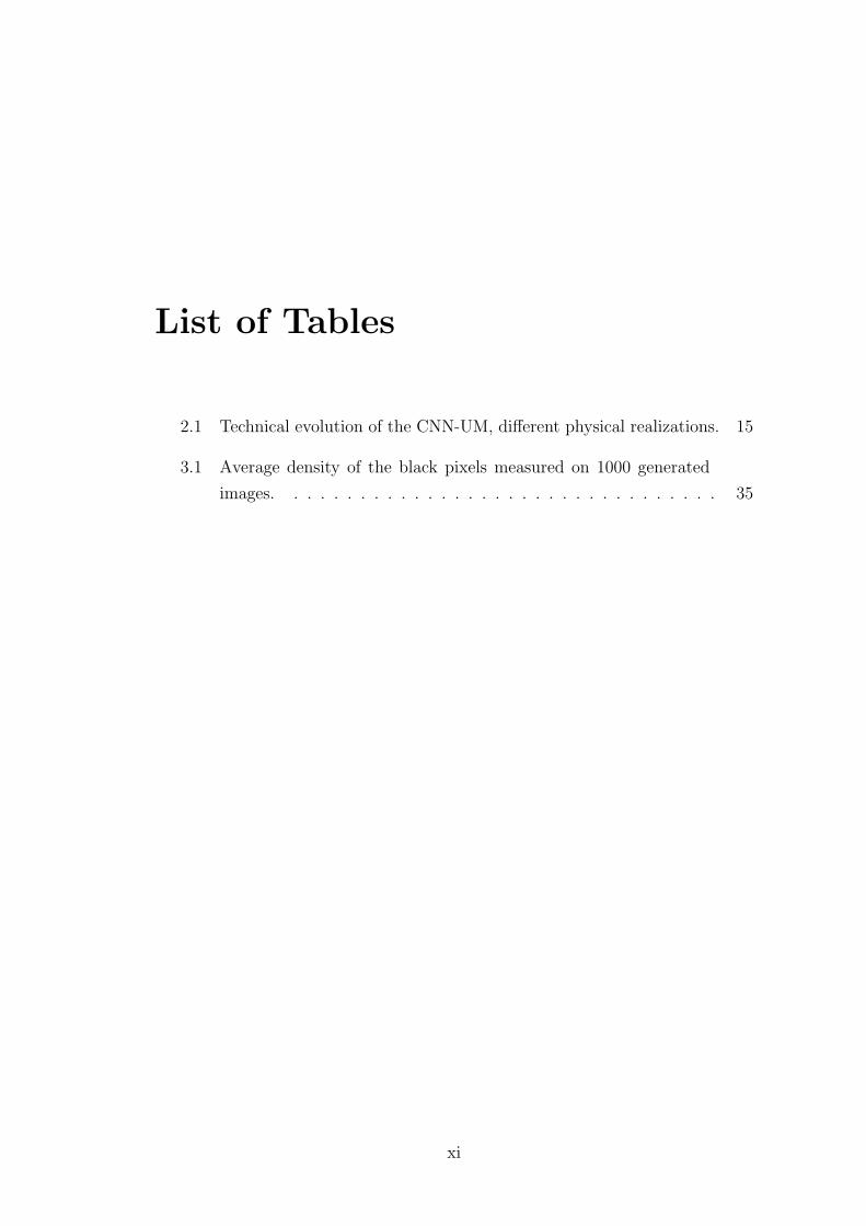
2.1 Technical evolution of the CNN-UM, different physical realizations. 15
3.1 Average density of the black pixels measured on 1000 generated
images. . . . . . . . . . . . . . . . . . . . . . . . . . . . . . . . . 35
xi


Chapter 1
Introduction
Many areas of sciences are facing problems concerning the computing power of
the presently available computers. Solving more and more complex problems,
simulating large systems, analyzing huge data sets for which even storing repre-
sents a problem, are just a few examples which reminds us that computing power
needs to keep up with its exponential growth, as expressed by Moore’s law [14].
We are aware however that this process can not continue much further solely with
the classical digital computer architecture, containing a few processors on a chip,
and new computational paradigms are necessary in order to keep up with the
increasing demands.
Progress in computation is always driven and deeply influenced by the avail-
able technology. After the breakthrough introduced by John Von Neumann’s
invention of digital stored programmable computers [15], for a long period com-
putation was approached by using discrete variables on one processor, and the
instructions were defined via arithmetic and Boolean logic. The revolution of
microprocessors made cheap computing power available almost for everyone. It
started in the 1970s and led to the profitable PC industry of the 1980s. Since
then a continuous increasing speed of the newly appearing processors has been
observed. This evolution of speed is strongly connected to the characteristic size
of the elements of the processors, which was constantly decreasing. Nowadays,
this process is slowing down due to the fact that atomic-size limit is very close
and the dissipation of a CMOS chip hits the ∼ 100 W limit. Since ∼ 2003 this
power dissipation limit saturated the clock frequency. Instead, the number of
1
2 1. INTRODUCTION
processors is increasing, leading also to a cellular, locally high-speed - globally
lower speed architecture [16, 17].
Another reason why the classical digital computers will need to be replaced
or at least supplemented, is due to the revolution of sensors of the 1990s, which
probably will lead to a new industry. Cheap micro-electro-mechanical systems,
different kind of sensors, like artificial eyes, nose, ears etc., are constantly appear-
ing and will be soon available. All these are producing analog signals waiting for
processing. Classical digital computing, even with a dozen or 20 cores, does not
fit well to this task.
Until recently, when thinking about computing, it was trivial that all data are
discrete variables, time is discrete, and the elementary instructions are defined on
a few discrete numbers (via arithmetic and Boolean logic units). The geometrical
position of the physical processors, if there were more than a single one, at all,
had no relevance. Nowadays, the scenario is drastically different. We can place
a million 8-bit microprocessors on a single 45 nm CMOS chip, the biggest super-
computer has a quarter million processors (the Blue Gene), and the new cellular
visual microprocessor chip (Q-Eye) contains 25k processors, each one hosting 4
optical sensors. Moreover, until recently, physical parameters, like wire delay and
power dissipation did not play a role in the algorithmic theory of computing [16].
These systems are much more complex than the classical parallel computers, so
the question arises: what will be the prototype architecture of the nano-scale
devices and systems, having, maybe, a million processors, and several TeraOPS
computing power, and what kind of algorithms could handle these systems?
In the light of the presently emerging quantitative neuroscience, it became
possible to understand the signal representation and processing in some parts of
our nervous system. Parallel with this a new and revolutionary different way
of computing is arising. The several thousands of microprocessors (cells) placed
on a single chip locally interacting with each other become similar to a layer of
neurons, imitating some basic principles of our nervous system. One suggested
prototype architecture for this unconventional computation is the Cellular Wave
Computer [18, 16, 17], a special case of it being the Cellular Nonlinear/Neural
Network Universal Machine (CNN-UM) [19, 20].

3
The history of CNN computing starts in 1988, when the theory of cellular neu-
ral/nonlinear networks (CNN) was presented [21]. Few years later a detailed plan
for a computer using cellular neural networks was developed. This is called CNN
Universal Machine (CNN-UM) [19] and is an analogic (analog+logic) computer
which has on its main processor several thousands of interconnected computa-
tional units (cells), working in parallel. Since then many experimental hardwares
were developed and tested [22, 23, 24]. As mentioned, the new chip Q-Eye, in-
cluded in the self-mantained camera computer, Eye-Ris [25], has 25000 processors,
each one hosting 4 optical sensors, it can capture 10000 frames/second, and it
consumes only 250 mW on a 30 mm2 chip. These chips can be easily connected to
digital computers and programmed with special languages. Although the CNN
computer is proved to be a universal Turing machine as well [26], its structure
and properties make it suitable mainly for some special complex problems, and
it is complementing and not replacing digital computers.
Most of the CNN-UM based chips are used and developed for fast image
processing applications [27]. The reason for this is that the cells can be used as
sensors (visual or tactile) as well. A CNN computer can work thus as a fast and
”smart” camera, on which the capturing of the image is followed in real time by
analysis [24]. As a computational physicist, I was convinced, that the physicist
community can also benefit from CNN based computers. It has been proved
in previous studies that this novel computational paradigm is useful in solving
partial differential equations [28, 29] and for studying cellular automata models
[30, 31]. All these applications result straightforwardly from the appropriate
spatial structure of the CNN chips. Moreover, the new nano-scale devices might
lead to new CNN like architectures.
During my Ph.D. studies my goal was to develope several new applications
related to statistical physics. The first of them was a realistic (true) random
number generator which can use the natural noise of the CNN chip for generating
binary random numbers [1] (see Chapter 3). This random number generator
served as a base for implementing different kind of stochastic simulations on the
CNN chip. In this aspect algorithms for the site-percolation problem and the
two-dimensional Ising model were developed and implemented on the ACE16K
chip [2] [5] (Chapter 4). In a more theoretical part of my research I also studied

4 1. INTRODUCTION
cellular nonlinear/neural networks with locally variable connections. I have shown
that a CNN on which the templates can be separately controlled for each cell
could be useful in efficiently solving NP-hard problems. As a specific problem,
energy minimization on two-dimensional spin-glasses was considered [3] (Chapter
5). As a last topic I studied a non-standard cellular nonlinear/neural network in
which the cells are simple, globally coupled oscillators communicating with light.
Although this is a first part of a longer project, interesting collective behavior
and weak synchronization phenomena were observed [6] (Chapter 6).

Chapter 2
Cellular neural/nonlinearnetworks and CNN computers
This chapter describes the structure and dynamics of Cellular Neural/Nonlinear
Networks (CNN) [21], including the standard CNN model. We also consider a
general description of CNN templates together with some important theorems.
The architecture and some of the physical implementations of the CNN Universal
Machine ([19]) are also presented. In the last section we briefly present some basic
applications realized on CNN computers.
2.1 Introduction
CNN computers are cellular wave computers [18] in which the core is a cellular
neural/nonlinear network (CNN), an array of analog dynamic processors or cells.
CNN was introduced by Leon O. Chua and Lin Yang in Berkeley, in 1988 [21],
as a new circuit architecture possessing some key features of neural networks:
parallel-signal processing and continuous-time dynamics, allowing real-time sig-
nal processing. CNN host processors are accepting and generating analog signals,
the time is continuous and the interaction values are also real numbers. These
analogic CNN computers are part of bio-inspired information technology. When
using this CNN dynamics model in a stored programmable and/or multilayer
architecture, they mimic the anatomy and physiology of some sensory and pro-
cessing organs (the retina for example). The computer architecture of cellular
neural/nonlinear networks is the CNN Universal Machine [20, 19], having various
5

62. CELLULAR NEURAL/NONLINEAR NETWORKS AND CNN
COMPUTERS
physical implementations [22, 23, 24, 25]. When implemented on a CMOS chip,
it is a fully-programmable stored-program dynamic array computer. Being now
commercially available, it represents an important step in information technology.
It can be embedded in a digital environment and offers a viable complement to
digital computing. Due to stored-program capability and analog-and-logic (ana-
logic) architecture the CNN-UM is superior to all mixed-mode circuits and neural
chips introduced before [32]. Digital computers are universal in the Turing sense,
which means, taking no time-limit, any algorithm on integers conceived by hu-
mans can be solved. The CNN Universal Machine is universal not only in the
Turing sense, but also on analog array signals [33, 18, 26]. Since 2003, the Inter-
national Technology Roadmap for Semiconductors (ITRS, published biannually)
considers CNN technology as one of the major emerging architectures (see also
the latest ITRS edition 2007).
2.2 Cellular neural/nonlinear networks
The cellular neural/nonlinear network was proposed by Leon O. Chua and Lin
Yang in 1988 [21] as a novel class of information processing system. It shares
some important features of neural networks: it is a large-scale nonlinear ana-
log circuit assuring parallel processing and continuous-time dynamics, all these
features allowing real-time signal processing. At the same time it is made of
regularly spaced circuit clones, called cells, which communicate with each other
only through nearest neighbors, like in a cellular automata.
2.2.1 The standard CNN model
A standard CNN architecture [21] consists of an M×N rectangular array of cells.
We will note with C(i, j) the cell in row i and column j. Each cell is directly
connected with its 4 nearest and 4 next-nearest neighbors (Fig. 2.1). These 8
cells define the first neighborhood of the cell. For a rigorous definition of the
neighborhood of a cell, one could say that the r-neighborhood of a cell Nr(i, j),
or the sphere of influence with radius r is
Nr(i, j) =
C(k.l)| max
i=1,M ;j=1,N|k − i| , |l − j| ≤ r
, (2.1)

2.2 Cellular neural/nonlinear networks 7
Figure 2.1: The lattice structure of the standard CNN.
r being a positive integer number. Another frequently used expression is the ”3×3
neighborhood” for r = 1, ”5× 5 neighborhood” for r = 2, ”7× 7 neighborhood”
for r = 3, etc.
Each cell is a small circuit made of a linear capacitor (C), an independent
current source (I), an independent voltage source (Eij), two linear resistors (Rx
and Ry) and a few voltage-controlled current sources, as shown in fig. 2.2. The
node voltage xij is called the state of the cell C(i, j), uij is the input voltage and
yij is the output voltage of the cell.
As observable from fig. 2.2 the input voltage has a constant value, which is
defined by the independent voltage source Eij:
uij = Eij. (2.2)
The state value xij is defined by the current source Iij, the linear capacitor C,
the linear resistor Rx and some linear voltage-controlled current sources. These
linear current sources are controlled by the voltages of the neighbor cells, and this
is how the coupling of cells is realized. There are two different types of coupling.

82. CELLULAR NEURAL/NONLINEAR NETWORKS AND CNN
COMPUTERS
Figure 2.2: The standard cell circuit.
Some linear current sources Ixu(i, j; k, l) are controlled by the input voltage ukl of
the neighbors C(k, l), others Ixy(i, j; k, l) get a feedback from the output voltages
ykl of neighbor cells:
Ixy(i, j; k, l) = A(i, j; k, l)ykl (2.3)
Ixu(i, j; k, l) = B(i, j; k, l)ukl. (2.4)
The feedback coupling parameters A(i, j; k, l) and input coupling parameters
B(i, j; k, l) can be used to change and control the strength of interactions be-
tween cells.
After the linear voltage controlled current sources are defined, one can write
up the state equation for the state voltage of cell C(i, j). Using the Kirchoff
equations and adding the current intensities in the node of the state voltage, this
state equation will be the following:
Cdxij(t)
dt= − 1
Rx
xij(t) +∑
C(k,l)∈Nr(i,j)
A(i, j; k, l)ykl(t) +
∑C(k,l)∈Nr(i,j)
B(i, j; k, l)ukl(t) + Iij. (2.5)

2.2 Cellular neural/nonlinear networks 9
Figure 2.3: The characteristic piecewise-linear function of the nonlinear controlledsource. This defines the output of the cell.
The output of the cell yij is determined by the nonlinear voltage-controlled cur-
rent source Iyx. This is the only non-linear element of the cell, it is a so called
piecewise-linear current source controlled by the state voltage of the cell:
Iyx =1
Ry
f(xij), (2.6)
f(x) =1
2(|x + 1| − |x− 1|). (2.7)
The function f is the characteristic function of the nonlinear controlled source
(Fig. 2.3). From this we can conclude that the output voltage yij = IyxRy (this
relation comes from the Kirchoff equation) will have the following form:
yij(t) = f(xij(t)) = 1/2(|xij(t) + 1| − |xij(t)− 1|). (2.8)
C and Rx will define the time-constant of the dynamics of the circuit: τ =
CRx, which is usually chosen to be 10−8-10−5 seconds. This parameter strongly
determines the speed of signal processing on CNN. Taking the time constant
τ = CRx = 1 (or simply measuring the time in units equal to this constant),
and denoting zij = Iij/C, also called the bias of the cell, we can write the state

102. CELLULAR NEURAL/NONLINEAR NETWORKS AND CNN
COMPUTERS
equation in a simpler form:
dxij(t)
dt= −xij(t) +
∑C(k,l)∈Nr(i,j)
A(i, j; k, l)ykl(t) +
+∑
C(k,l)∈Nr(i,j)
B(i, j; k, l)ukl(t) + zij. (2.9)
Eq. 2.9 can be considered, in general, as the canonical equation of the standard
CNN dynamics.
The output voltages depend on the state voltages (eq. 2.8), the input voltages
and the bias are constant in time, so we have a coupled system of differential equa-
tions with variables xij. The dynamics of the system is governed by parameters
A(i, j; k, l), B(i, j; k, l), zij. This group of parameters will be called a template.
The template can be used for defining different operations on the CNN.
Because the CNN is defined on a two-dimensional array and the output values
of the cells are always in the range of [−1, 1], we can illustrate the state of the
CNN as a grayscale image, on which pixels with value −1 are white, pixels with
value 1 are black.
2.2.2 CNN templates
As seen in eq. 2.9, the state of a cell depends on interconnection weights between
the cell and its neighbors. These parameters are expressed in the form of the
template A(i, j; k, l), B(i, j; k, l), zij.In most cases space-invariant templates are used. This means, for example,
that A(i, j; i + 1, j) is the same for all (i, j) coordinates. In such way, on the
two-dimensional CNN chip, all the A couplings are defined by a single 3 × 3
matrix, called the feed-back matrix. The whole system can be characterized by
this feed-back matrix, a control matrix (of parameters B) and the bias. Totally,
9+9+1 = 19 parameters are needed to define the whole, globally valid, template
(A,B,z):
A =
a−1,−1 a−1,0 a−1,1
a0,−1 a0,0 a0,1
a1,−1 a1,0 a1,1
, B =
b−1,−1 b−1,0 b−1,1
b0,−1 b0,0 b0,1
b1,−1 b1,0 b1,1
, z. (2.10)

2.2 Cellular neural/nonlinear networks 11
On the latest version of the CNN chips (ACE16k [23], Q-Eye [25]) the z(i, j)
parameter can be already locally varied. In chapter 5 we will also use space-
variant CNN templates, in which all connection parameters are separately defined.
2.2.2.1 Important theorems
In their first paper which introduced the cellular neural networks, Chua and
Yang [21] presented some important theorems concerning the dynamic range and
stability of cellular neural networks. Some of these will be used during this work,
so we shortly present them here.
Theorem 1: All states xij in a cellular neural network are bounded for any
time t, and the bound is:
xmax = 1 + Rx |I|+ Rx · maxi = 1, M
j = 1, N
∑C(k,l)∈Nr(i,j)
(|A(i, j; k, l)|+ |B(i, j; k, l)|)
.(2.11)
This formula can be obtained from the state equation of CNN. The fact that all
voltages will remain bounded is crucial for the realization of the circuits.
Other important theorems are dealing with the stability of CNN. In order to
use these cellular neural networks in computing, the output of the cells should
always converge to a constant steady state. If this would not be satisfied we
would observe fluctuating and constantly changing images, and consequently we
would not get an exact well defined result to the implemented algorithms. It
is thus important to analyze the convergence properties of these systems. Here
we only mention some important theorems, the rigorous demonstrations can be
found in [21]. The convergence of the system can be studied defining the following
Lyapunov function, which behaves like a generalized energy of the system:
E(t) = −1
2
∑(i,j)
∑(k,l)
A(i, j; k, l)yij(t)ykl(t) +1
2Rx
∑(i,j)
yij(t)2 −
−∑(i,j)
∑(k,l)
B(i, j; k, l)yij(t)ukl −∑(i,j)
Iyij(t). (2.12)
We should observe that in the [−1, 1] region, where the state values and output
values are equal, xij = yij, this function is equivalent with the energy of the
122. CELLULAR NEURAL/NONLINEAR NETWORKS AND CNN
COMPUTERS
system, obtained by applying the work-energy theorem (the derivative of this
function: dE/dyij is the same as −dxij/dt in equation 2.5). The reason why this
Lyapunov function is used instead of the rigorously defined energy function, is
that it contains only the output and input values of the cells. This function is
also similar to the one used by Hopfield in [34].
Theorem 2: a)The function E(t) is bounded for all t:
maxt|E(t)| ≤ Emax =
1
2
∑(i,j)
∑(k,l)
|A(i, j; k, l)|+∑(i,j)
∑(k,l)
|B(i, j; k, l)|+
+MN
(1
2Rx
+ |I|)
. (2.13)
b)The function E(t) is a monotone-decreasing function:
dE(t)
dt≤ 0. (2.14)
c)For any given input and any initial state, for all (i, j) we have:
limt→∞
E(t) = const., limt→∞
dE(t)
dt= 0, (2.15)
limt→∞
yij(t) = const., limt→∞
dyij(t)
dt= 0. (2.16)
All these mathematical statements can be proved using the state equation of the
CNN and the first theorem, which says that all states remain bounded (see [21]).
From these theorems we can see that the system will always converge to a final
steady state.
Another important property of the system is that: when A(i, j; i, j) > 1Rx
in
eq. 2.5, or A(i, j; i, j) > 1 in the case of state equation 2.9 (in which time is
already defined by taking τ = CRx = 1 as unit) , the output of the system will
always be a binary image: limt→∞ yij(t) = ±1. This property is useful, when we
want to design templates for different tasks.
2.3 The CNN Universal Machine
After the theory of cellular neural networks was published in 1988 by Chua and
Yang [21], the architecture for the CNN Universal Machine was developed in 1993
2.3 The CNN Universal Machine 13
[19] . This CNN-UM can be embedded in digital environment offering a viable
complement and in some cases an alternative to digital computing. This machine
has stored-program capability and analog-and-logic architecture. After many
successful implementations of CNN [35], the CNN Universal chip was announced
in 1994 [36]. Since then many other chips with stored-program capability have
been developed [22, 23, 25].
2.3.1 The architecture of the CNN-UM
The architecture of the CNN-UM [19, 27] follows mainly the theory already pre-
sented. On each site of a square lattice we have an extended cell (Fig. 2.4)
with a nucleus containing a circuit similar to the one presented on fig.2.2. The
difference in this circuit is that we have some switches which are necessary for
using the different local memories, but qualitatively the role of this circuit is the
same as described. Beside the nucleus presented in the theory, the cells have
local analog memories (LAM) - storing real values (grayscale pixels), local logic
memories (LLM) - storing binary values. Local memories are very important
when implementing algorithms, because many tasks can be solved only with sev-
eral consecutive templates, and the intermediate results need to be stored. The
local analog output unit (LAOU) is a multiple-input single-output analog device
having the same functions for continuous values as the local logic unit (LLU) for
logic values, namely it combines more local values into a single output value. It
can be used for some simple functions, like addition. The local communication
and control unit (LCCU) receives the programming instructions in each cell from
the global analog programming unit (GAPU) [27].
Beside the array of the extended cells we need some global units to control
the whole CNN-UM (Fig. 2.5). The GAPU is this global conductor, from where
each cell gets the instructions: namely the template values, the logic instructions
for the LLU, and the switch configuration for the nucleus circuit. So the GAPU
must have registers for these three types of elements. (as shown on fig. 2.5)
• The analog program register (APR)
• The logic program register (LPR)

142. CELLULAR NEURAL/NONLINEAR NETWORKS AND CNN
COMPUTERS
Figure 2.4: The extended cell.
• And the switch configuration register (SCR).
Beside these registers the global analogic control unit (GACU) is the part of the
GAPU which controls the whole system. The global wire means that although
the cells are connected with their neighbors each of them must be also directly
connected with the global unit. The global clock is essential for programming
because we need all transient of cells decay in a specified clock cycle. Otherwise
cells cannot be synchronized.
The CNN universal machine having the presented architecture [20, 27]:
• contains the minimum number of component types,
• provides stored programmable spatiotemporal array computing,
• is universal in two senses [26]:
– as spatial logic it is equivalent to a Turing machine, as local logic it
can implement any local Boolean function.
– as a nonlinear dynamic operator working on array signals.

2.3 The CNN Universal Machine 15
Figure 2.5: The structure of the CNN universal machine.
This is the reason why the CNN-UM is a common computational paradigm [20] for
many different fields of spatiotemporal computing (like retina models, reaction-
diffusion equations etc).
2.3.2 Physical implementations
The physical implementations of these computers are numerous and widely dif-
ferent: mixed-mode CMOS, emulated digital CMOS, FPGA, and also optical.
For practical purposes the most promising applications are for image processing,
Name Year Size— 1993 12× 12ACE440 1995 20× 22POS48 1997 48× 48ACE4k 1998 64× 64CACE1K 2001 32× 32× 2ACE16k 2002 128× 128XENON 2004 128× 96EYE-RIS 2007 176× 144
Table 2.1: Technical evolution of the CNN-UM, different physical realizations.

162. CELLULAR NEURAL/NONLINEAR NETWORKS AND CNN
COMPUTERS
robotics or sensory computing purposes [37], so the main practical drive in the
mixed-mode implementations was to build a visual microprocessor [27]. In the
last decades the size of the engineered chips was constantly growing (see Ta-
ble 2.1), the new cellular visual microprocessor EYE-RIS [25] for example has
176 × 144 processors, each cell hosting also 4 optical sensors. Parallel with in-
creasing the lattice size of the chips, engineers are focusing also on developing
multi-layered, 3 dimensional chips as well.
In my experiments the ACE16k chip [23] included in the Bi-iv2 [24] system was
used (Fig. 2.6). The Bi-i v2 is a device developed specially for image processing
purposes. The central component of the Bi-i is a high performance digital signal
processor (DSP) with 600MHz clock, the CNN chip is connected to this. The cells
of the included chip are also equipped with photosensors, so the whole system can
be used as a fast camera. It can capture more thousands of frames per second,
which can be processed and analyzed in real-time on the CNN chip.
The native programming language for Bi-i is the AnaLogic Macro Code (AMC).
This language and software was developed specially for CNN programming. Pro-
gram development is supported by a syntax-highlight editor, which invokes the
AMC compiler. The editor and compiler are part of the Aladdin software [38].
This language is not designed for large projects, but is very effective for small
applications and especially for programming these chips, which are still in exper-
imental phase. One can control which memories to use at each operation, this
way the computational time can be more efficiently optimized, than in a high
level language. There are also other ways for programming the Bi-i: the SDK
(Software Development Kit), which is a C++ programming library for develop-
ing Bi-i applications; and the API (Application Program Interface), which is a
software interface for applications only interacting with the Bi-i.
2.4 Applications of CNN computing
In this section we present some examples of the most common applications re-
alized on CNN computers. Most of these are useful image processing functions
[39, 37]. Apart of these also some partial differential equations [28, 29] and cel-
lular automata models [30] can be easily implemented. The CNN templates and

2.4 Applications of CNN computing 17
Figure 2.6: The Bi-i v2.
the simulated results will be presented without analysis. For more information
please consult the indicated references.
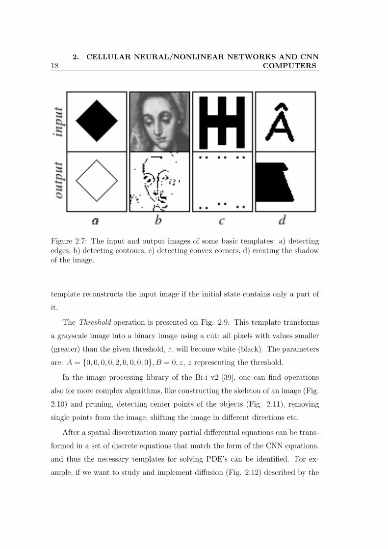
On Fig. 2.7 we present the input images and results of some basic templates
used in many image processing algorithms:
a) The Edge template:
A = 0, 0, 0, 0, 1, 0, 0, 0, 0, B = −1,−1,−1,−1, 8,−1,−1,−1,−1, z = −1,
finds the edges on a binary input image.
b) The Contour template:
A = 0, 0, 0, 0, 2, 0, 0, 0, 0, B = −1,−1,−1,−1, 8,−1,−1,−1,−1, z = −0.5,
finds the contours on a grayscale input image.
c) The Corner template:
A = 0, 0, 0, 0, 1, 0, 0, 0, 0, B = −1,−1,−1,−1, 4,−1,−1,−1,−1, z = −5,
detects convex corners on the input image.
d) The Shadow template:
A = 0, 0, 0, 0, 2, 2, 0, 0, 0, B = 0, 0, 0, 0, 2, 0, 0, 0, 0, z = 0, creates the shadow
of the input image
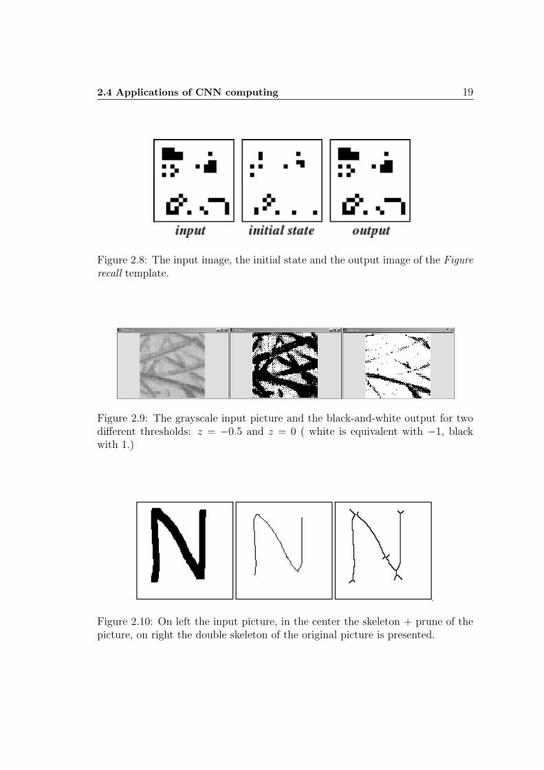
On Fig. 2.8 the Figure recall template is illustrated:
A = 0.5, 0.5, 0.5, 0.5, 4, 0.5, 0.5, 0.5, 0.5, B = 0, 0, 0, 0, 4, 0, 0, 0, 0,z = 3. This
182. CELLULAR NEURAL/NONLINEAR NETWORKS AND CNN
COMPUTERS
Figure 2.7: The input and output images of some basic templates: a) detectingedges, b) detecting contours, c) detecting convex corners, d) creating the shadowof the image.
template reconstructs the input image if the initial state contains only a part of
it.
The Threshold operation is presented on Fig. 2.9. This template transforms
a grayscale image into a binary image using a cut: all pixels with values smaller
(greater) than the given threshold, z, will become white (black). The parameters
are: A = 0, 0, 0, 0, 2, 0, 0, 0, 0, B = 0, z, z representing the threshold.
In the image processing library of the Bi-i v2 [39], one can find operations
also for more complex algorithms, like constructing the skeleton of an image (Fig.
2.10) and pruning, detecting center points of the objects (Fig. 2.11), removing
single points from the image, shifting the image in different directions etc.
After a spatial discretization many partial differential equations can be trans-
formed in a set of discrete equations that match the form of the CNN equations,
and thus the necessary templates for solving PDE’s can be identified. For ex-
ample, if we want to study and implement diffusion (Fig. 2.12) described by the
2.4 Applications of CNN computing 19
Figure 2.8: The input image, the initial state and the output image of the Figurerecall template.
Figure 2.9: The grayscale input picture and the black-and-white output for twodifferent thresholds: z = −0.5 and z = 0 ( white is equivalent with −1, blackwith 1.)
Figure 2.10: On left the input picture, in the center the skeleton + prune of thepicture, on right the double skeleton of the original picture is presented.

202. CELLULAR NEURAL/NONLINEAR NETWORKS AND CNN
COMPUTERS
Figure 2.11: Results of the centroid function. We see the input image in thefirst window, the output image contains only the center points, and in the thirdwindow the number of objects is printed.
two-dimensional heat-equation with form
δu(x, y, t)
δt= c∇2u(x, y, t), (2.17)
we first make a spatial discretization with equidistant steps h in both directions
of the plane (meaning xij(t) = u(ih, jh, t)). The following template will be im-
mediately identified:
A =
0 ch2 0
ch2 1− 4c
h2c
h2
0 ch2 0
, B = 0, z = 0. (2.18)
Given the parallel structure of CNN, it is also suitable for implementing cel-
lular automata models. Depending on the basic rule of the cellular automata it
can be implemented on the CNN with one or more consecutive templates. The
effectiveness of CNN in handling cellular automata models consists in parallel
processing: the rule is performed in each cell at the same time. Some basic ex-
amples are the dilation and erosion processes. An example for erosion is presented
on Fig. 2.13. Many other templates used in image processing, are also simple
cellular automata models (shadowing, shifting, etc.) Some algorithms for more
complicated cellular automata were also developed. One example is given by
Cruz and Chua [30], who are using the CNN paradigm for modeling population

2.4 Applications of CNN computing 21
Figure 2.12: Result of continuous diffusion after t = 0, 10, 20 τ time (the unit τis the time-constant of the CNN).
Figure 2.13: The result of erosion after t = 0, 6, 12 τ time.
dynamics. A social segregation model is presented in form of a cellular automata
and is converted into a CNN problem, by giving the appropriate templates.
As mentioned already, in the Bi-i the CNN chip has photo sensors in each
cell and can work like a very fast camera, this representing another important
application possibility [24]. If the light intensity is strong, a small capturing time
is enough (even a few microseconds). For making a video, the frame rate will be
limited only by the time needed for moving the picture from the CNN chip to
the DSP. But even this way, the frame rate can attain more thousands of frames
per second. Comparing to usual cameras (working usually with 25-30 frames/s)
this is a very high speed, and this feature of the Bi-i assures many interesting
applications. Applications of this type might be useful in robotics, medical image
analysis, or even in scientific experiments recording fast phenomena in nature.


Chapter 3
Generating realistic, spatiallydistributed random numbers onCNN
In this chapter we present a realistic (true) random number generator (RNG)
which uses the natural noise of the CNN-UM chip. Generating random numbers is
crucial for many applications related to physics, especially stochastic simulations.
First we present an algorithm for generating binary values with 1/2 probability
of 0 (white pixels) and 1 (black pixels), then an algorithm for generating binary
values with any p probability of the black pixels will be presented. Experiments
were made on the ACE16K chip with 128× 128 cells [1] [5].
3.1 Introduction
While computing with digital processors, the ”world” is deterministic and dis-
cretized, so in principle there is no possibility to generate random events and thus
really random numbers. The implemented random number generators are in fact
pseudo-random number generators working with some deterministic algorithm,
and it is believed that their statistics approximates well real random numbers.
Pseudo-randomness and the fact that the random number series is repeatable
can be helpful sometimes, it makes easier debugging Monte Carlo (MC) type
programs and can be a necessary condition for implementing specific algorithms.
However, we should be always aware about their limitations. For example, in
23

243. GENERATING REALISTIC, SPATIALLY DISTRIBUTED
RANDOM NUMBERS ON CNN
solving complicated statistical physics problems with large ensemble averages,
the fact that the RNG is deterministic and can have a finite repetition period
limits the effectiveness of the statistics. One can immediately realize, that a first
advantage of the programmable analog architecture embedded in the CNN-UM
is that the simple, fully deterministic and discretized ”world” is lost, noise is
present, and there is thus possibility for generating real random numbers. Here,
first we present a realistic random number generator which uses the natural noise
of the CNN-UM chip and generates random binary images with a uniform distri-
bution of the white and black pixels. After that a method for generating binary
images with any given probability of the black pixels will be described. The
advantages and perspectives of these methods are discussed in comparison with
classical digital computers.
3.2 Generating random binary values with 1/2
probability
3.2.1 Pseudo-random generators on CNN
There are relatively few papers presenting or using random number generators
(RNG) on the CNN Universal Machine [40, 31, 41, 42]. The already known and
used ones are all pseudo-random number generators based on chaotic cellular au-
tomaton (CA) type update rules. According to Wolfram’s classification scheme
the III. class of cellular automata are called chaotic, because from almost all pos-
sible initial states they lead to aperiodic (”chaotic”) patterns. After sufficiently
many time steps, the statistical properties of these patterns are typically the same
for almost all initial states. In particular, the density of non-zero sites typically
tends to a fixed non-zero value. This class has the biggest chance to serve as a
good random number generator, but still these RNGs are, in reality, deterministic
and for many initial conditions they might have finite repetition periods.
All the pseudo RNGs developed on the CNN-UM up to the present are gen-
erating binary images with equal 1/2 probability of the black and white pixels
(logical 1 and 0 are generated with the same probability). Most of them are used
mainly in cryptography [31] and watermarking on pictures [40]. One of the most

3.2 Generating random binary values with 1/2 probability 25
Figure 3.1: The truth-table of the cellular automaton. The result of each 25 = 32pattern is represented by the colour of the frame. Grey cells can have arbitraryvalues.
263. GENERATING REALISTIC, SPATIALLY DISTRIBUTED
RANDOM NUMBERS ON CNN
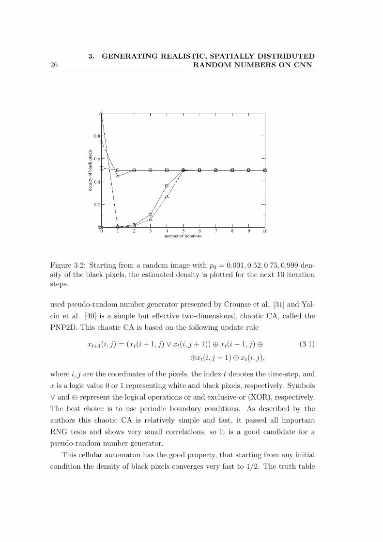
Figure 3.2: Starting from a random image with p0 = 0.001, 0.52, 0.75, 0.999 den-sity of the black pixels, the estimated density is plotted for the next 10 iterationsteps.
used pseudo-random number generator presented by Crounse et al. [31] and Yal-
cin et al. [40] is a simple but effective two-dimensional, chaotic CA, called the
PNP2D. This chaotic CA is based on the following update rule
xt+1(i, j) = (xt(i + 1, j) ∨ xt(i, j + 1))⊕ xt(i− 1, j)⊕ (3.1)
⊕xt(i, j − 1)⊕ xt(i, j),
where i, j are the coordinates of the pixels, the index t denotes the time-step, and
x is a logic value 0 or 1 representing white and black pixels, respectively. Symbols
∨ and ⊕ represent the logical operations or and exclusive-or (XOR), respectively.
The best choice is to use periodic boundary conditions. As described by the
authors this chaotic CA is relatively simple and fast, it passed all important
RNG tests and shows very small correlations, so it is a good candidate for a
pseudo-random number generator.
This cellular automaton has the good property, that starting from any initial
condition the density of black pixels converges very fast to 1/2. The truth table
3.2 Generating random binary values with 1/2 probability 27
of the cellular automaton can be seen on fig. 3.1. From the 25 = 32 possible
patterns, there are 16 resulting in black (1) and 16 resulting in white (0) pixels.
This is the reason why the density converges to 1/2. If we presume that the
image at time step t is a random image with a uniform density, p, of the black
pixels, we can also estimate the new density obtained after one iteration using
the following equation:
pt+1 = 3p4t (1− pt) + 7p3
t (1− pt)2 + p2
t (1− pt)3 + 5pt(1− pt)
4 (3.2)
The equation comes from simply adding the probabilities of the 16 patterns re-
sulting in black (1). On fig. 3.2 the density values after more iterations are
plotted, starting from different initial conditions (p0 = 0.001, 0.52, 0.75, 0.999).
The results show that the density reaches the 1/2 in less then 10 iterations. This
simple estimation is valid only if we start from a random image with uniform
distribution, but the convergence is fast also in other cases.
3.2.2 A realistic RNG using the natural noise of the CNNchip
Our goal is to take advantage on the fact that the CNN-UM chip is a partly
analog device, and to use its natural noise for generating more realistic random
numbers. This would assure an important advantage relative to digital computers,
especially in Monte Carlo type simulations. The natural noise of the CNN-UM
chip - mainly thermal or Nyquist noise - is usually highly correlated in space
and time, so it can not be used directly to obtain random binary images. Our
method is based thus on a chaotic cellular automaton (CA) perturbed with the
natural noise of the chip after each time step. As it will be shown later, due to
the used chaotic cellular automaton, the correlations in the noise will not induce
correlations in the generated random image. The real randomness of the noise
will kill the deterministic properties of the chaotic cellular automaton.
As starting point a good pseudo-random number generator implemented on
the CNN-UM, the chaotic CA presented in the previous section, called PNP2D
was chosen [31, 40]. Our method for transforming this into a realistic RNG
is relatively simple. After each time step the P (t) result of the chaotic CA is

283. GENERATING REALISTIC, SPATIALLY DISTRIBUTED
RANDOM NUMBERS ON CNN
Figure 3.3: The flowchart for the algorithm that generates binary images with1/2 probability of the black pixels.

3.2 Generating random binary values with 1/2 probability 29
perturbed with a noisy N(t) binary picture (array) so that the final output is
given as:
P ′(t) = P (t)⊕N(t). (3.3)
The symbol ⊕ stands again for the logic operation exclusive-or, i.e. pixels which
are different on the two pictures will become black (logic value 1). This way for
all pixels which are white (0) on the N(t) image, the P ′(t) will be the same as
P (t), and for all pixels which are black (1) on N(t), the P ′(t) will be the inverse of
P (t). This assures that no matter how N(t) looks like, the density of black pixels
remains mainly the same 1/2. Fluctuations in the density can appear, but using
a noisy images with very few black pixels (typically 5 - 10) these fluctuations are
small. As shown in the previous subsection the properties of the chaotic cellular
automaton assure that in the next step the density will again converge to 1/2
(Fig. 3.2). So this perturbation just slightly sidetracks the chaotic CA from the
original deterministic path, but all the good properties of the pseudo-random
number generator and the 1/2 density of the pixels will be preserved.
The N(t) noisy picture is obtained by the following simple algorithm. All
pixels of a gray-scale image are filled up with a constant value a and a cut is
realized at a threshold a + z, where z is a relatively small value. In this manner
all pixels which have smaller value than a+z will become white (logic value 0) and
the others black (logic value 1). Like all logic operations, this threshold operation
can also be easily realized on the CNN-UM (see Chapter 2). Due to the fact that
in the used CNN-UM chip the CNN array is an analog device, there will always
be natural noise on the grayscale image. Choosing thus a proper z value one can
generate a random binary picture with few black pixels. Since the noise is time
dependent and generally correlated in time and space, the N(t) pictures might
be strongly correlated but will fluctuate in time. These time-like fluctuations can
not be controlled, these are caused by real stochastic processes in the circuits of
the chip and are the source of a convenient random perturbation for our RNG
based on a chaotic CA.
The flowchart of the algorithm is shown on fig. 3.3. Light gray boxes represent
the steps of the cellular automaton, dark gray boxes are the steps of perturbing
the result with the noise of the chip. The used local memories are also indicated.

303. GENERATING REALISTIC, SPATIALLY DISTRIBUTED
RANDOM NUMBERS ON CNN
Figure 3.4: Two consecutive random binary images with p = 1/2 probability ofthe black pixels. The images were generated on the ACE16K chip by using thepresented method.
When two local memories are given for the output, it means that the result is
copied in both memories. Symbols ∨ and ⊕ stand again for the operations OR
and XOR, respectively.
3.2.3 Numerical results
We implemented and tested the algorithm on the ACE16K chip [23], with 128×128 cells, included in a Bi-i v2 [24], using the Aladdin software [38]. We have
chosen the values a = 0.95 and z = −0.012. We observed that the noise is bigger
when a is close to 1, and that was the reason why we have chosen a = 0.95. The
motivation for the negative z value is the following. Our experiments revealed a
relatively strong negative noise on grayscale images. Due to this negative noise,
once a grayscale picture with a constant a value (0 < a < 1) is generated, the
measured average pixel value on the picture will always be smaller than a. The
chosen small negative value of z ensured getting an N(t) array with relatively
few black pixels. In case the noise on the grayscale picture is different (a different
chip for example) one will always find another proper value for z.
On the ACE16k chip we could not use periodic boundary conditions, instead
fixed boundary conditions were applied. This affects in a considerable manner
3.2 Generating random binary values with 1/2 probability 31
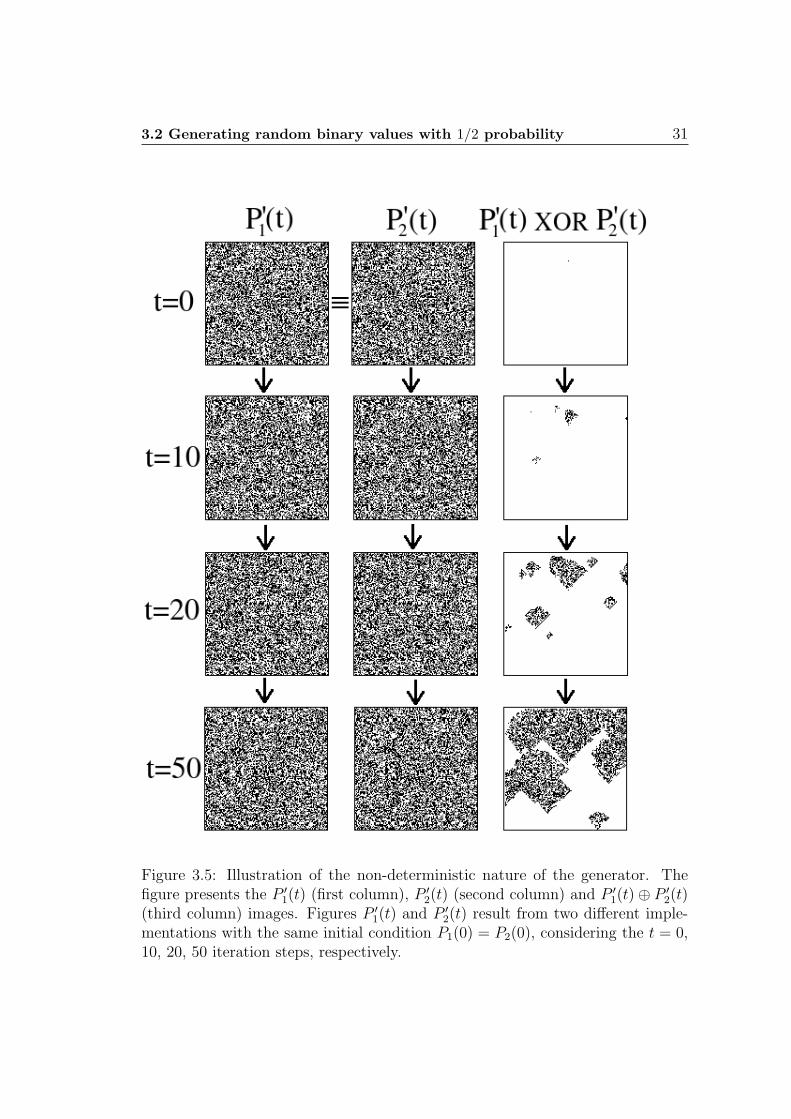
Figure 3.5: Illustration of the non-deterministic nature of the generator. Thefigure presents the P ′
1(t) (first column), P ′2(t) (second column) and P ′
1(t)⊕ P ′2(t)
(third column) images. Figures P ′1(t) and P ′
2(t) result from two different imple-mentations with the same initial condition P1(0) = P2(0), considering the t = 0,10, 20, 50 iteration steps, respectively.

323. GENERATING REALISTIC, SPATIALLY DISTRIBUTED
RANDOM NUMBERS ON CNN
only the boundary (i = 1, L or j = 1, L) rows and columns, which should not be
counted as part of the random image.
Two consecutive random images generated by this method using the men-
tioned a and z parameters are shown in Fig. 3.4. The density of the pixels was
measured on 1000 consecutive images and the average density was 0.4995. Cor-
relation tests were also performed. Normalized correlations in space between the
first neighbors were measured between 0.05− 0.2%, correlations in time between
consecutive steps were between 0.3− 0.5%.
Perturbing the CA with this noise assures also that starting from the same
initial state our RNG will yield different results P ′1(t), P ′
2(t), P ′3(t) etc., after
the same time-steps. Starting from the same initial condition (initial random
binary picture P1(0) = P2(0)) on Fig. 3.5 we compare for several time steps
the generated patterns. On this figure we plot the separate images, P ′1(t) (first
column), P ′2(t) (second column), and the image resulting from an XOR operation
performed on the P ′1(t) and P ′
2(t) pictures. In case of a simple deterministic
CA this operation would yield a completely white image for any time step t. As
visible from Fig. 3.5 in our case almost the whole picture is white in the beginning
showing that the two results are almost identical, but as time passes the small
N(t) perturbation propagates over the whole array and generates completely
different binary patterns. For t > 70 time-steps the two results are already
totally different.
We also compared the speed of the above presented RNG with RNGs under
C++ on normal digital computers, working on a RedHat 9.0 LINUX operating
system. In our experiments the necessary time for generating a new and roughly
independent random binary image on the ACE16K (350 nm technology) chip is
roughly 116µs. This means that for one single random binary value we need
116/L2µs, where L is the lattice size of the chip. In our case L = 128, so the
time needed for one random binary value is roughly 7ns. On a Pentium 4, 2.8
GHz machine (90 nm technology) this time is approximately 33ns. We can see
thus that parallel processing makes CNN-UM already faster, and considering the
natural trend that lattice size of the chip will grow, this advantage will amplify
in the future. The estimated computation time for one random binary value as a

3.3 Generating binary values with arbitrary p probability 33
Figure 3.6: Computational time needed for generating one single binary randomvalue on a Pentium 4 computer with 2.8GHz and on the used CNN-UM chip,both as a function of the CNN-UM chip size. Results on the actual ACE16K chipwith L=128 is pointed out with a bigger circle. The results for L > 128 sizes areextrapolations.
function of chip size and in comparison with a Pentium 4, 2.8 GHz PC computer
is plotted in Fig. 3.6.
3.3 Generating binary values with arbitrary p
probability
Up to now we considered that black and white pixels (1 and 0) must be generated
with equal, 1/2, probabilities. For the majority of the Monte Carlo methods this
is however not enough, and one needs to generate binary values with any arbitrary
probability p. On digital computers this is done by generating a real value in the
interval [0, 1] with a uniform distribution and making a cut at p. Theoretically it
is possible to implement similar methods on CNN-UM by generating a random
gray-scale image and making a cut-off at a given value. However, on the actual
chip it is extremely hard to achieve a gray-scale image with a uniform distribution
of the pixel values between 0 and 1 (or −1 and 1). Our solution for generating
a random binary image with p probability of the black pixels is by using more

343. GENERATING REALISTIC, SPATIALLY DISTRIBUTED
RANDOM NUMBERS ON CNN
independent binary images with p = 1/2 probability of the black pixels. We
reduce thus this problem, to the problem already solved in the previous section.
3.3.1 The algorithm
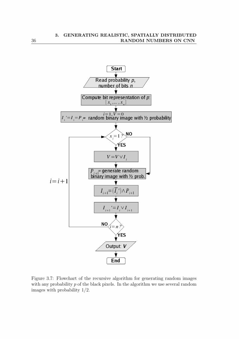
Let p be a number between 0 and 1,
p =8∑
i=1
xi · 1/2i, (3.4)
represented here on 8 bits by the xi binary values. One can approximate a random
binary image with any fixed p probability of the black pixels, by using 8 images
Ii, with probabilities pi = 1/2i, i ∈ 1,. . . ,8 of the black pixels and satisfying the
condition that Ii ∧ Ij = ∅ (relative to the black pixels) for any i 6= j ∈ 1,. . . ,8.Symbol ∧ stands for the operation AND. Once these 8 images are generated one
just have to unify (perform OR operation) all Ii images for which xi = 1 in the
expression of p (Eq. 3.4 ).
Getting these 8 basic Ii images is easy once we have 8 independent images
(Pi) with p = 1/2 probabilities of the black pixels. Naturally
I1 = P1, (3.5)
where P1 is the first basic image with 1/2 probability of the black pixels. The
second image with 1/4 probability of the black pixels is generated as:
I2 = I1 ∧ P2, (3.6)
where Ii denotes the negative of image Ii (I = NOT I). In this manner the
probability of black pixels on this second image I2 will be p2 = p1 · p1 = 1/4 and
condition I1 ∧ I2 = ∅ is also satisfied. Adding now the two images I1 and I2 we
obtain an image with 3/4 density of black pixels:
I ′2 = I1 ∨ I2. (3.7)
This I ′2 image is used than to construct I3:
I3 = I ′2 ∧ P3. (3.8)
3.3 Generating binary values with arbitrary p probability 35
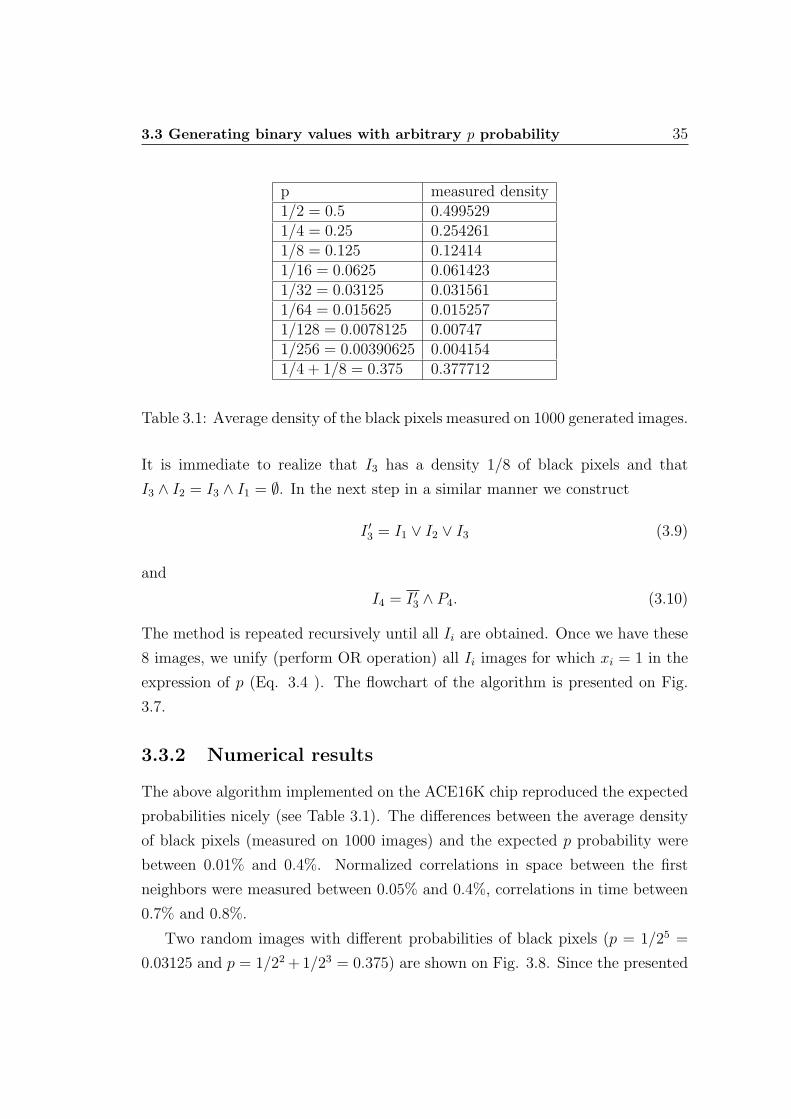
p measured density1/2 = 0.5 0.4995291/4 = 0.25 0.2542611/8 = 0.125 0.124141/16 = 0.0625 0.0614231/32 = 0.03125 0.0315611/64 = 0.015625 0.0152571/128 = 0.0078125 0.007471/256 = 0.00390625 0.0041541/4 + 1/8 = 0.375 0.377712
Table 3.1: Average density of the black pixels measured on 1000 generated images.
It is immediate to realize that I3 has a density 1/8 of black pixels and that
I3 ∧ I2 = I3 ∧ I1 = ∅. In the next step in a similar manner we construct
I ′3 = I1 ∨ I2 ∨ I3 (3.9)
and
I4 = I ′3 ∧ P4. (3.10)
The method is repeated recursively until all Ii are obtained. Once we have these
8 images, we unify (perform OR operation) all Ii images for which xi = 1 in the
expression of p (Eq. 3.4 ). The flowchart of the algorithm is presented on Fig.
3.7.
3.3.2 Numerical results
The above algorithm implemented on the ACE16K chip reproduced the expected
probabilities nicely (see Table 3.1). The differences between the average density
of black pixels (measured on 1000 images) and the expected p probability were
between 0.01% and 0.4%. Normalized correlations in space between the first
neighbors were measured between 0.05% and 0.4%, correlations in time between
0.7% and 0.8%.
Two random images with different probabilities of black pixels (p = 1/25 =
0.03125 and p = 1/22 +1/23 = 0.375) are shown on Fig. 3.8. Since the presented
363. GENERATING REALISTIC, SPATIALLY DISTRIBUTED
RANDOM NUMBERS ON CNN
Figure 3.7: Flowchart of the recursive algorithm for generating random imageswith any probability p of the black pixels. In the algorithm we use several randomimages with probability 1/2.

3.3 Generating binary values with arbitrary p probability 37
Figure 3.8: Random binary images with p = 0.03125 (left) and p = 0.375 (right)probability of black pixels. Both of them were obtained on the ACE16K chip.
method is based on our previous realistic RNG the images and binary random
numbers generated here are also non-deterministic.
The speed of the algorithm depends in a great measure on the probability
p. For example, if the biggest index for which xi = 1 is only 3, we need only 3
independent random images (Pi) and also the recursive part of the algorithm is
shorter. In the case when we need 8 random images, the algorithm is at least
8 times slower than for the p = 1/2 case. However, in general we rarely need 8
images. It worth mentioning also, that the possible values of p can be varied in a
more continuous (smooth) manner, if p is represented not on 8 but on arbitrary n
bits. In this manner one has to generate n binary images and the computations
on these pictures will become also more time-costly.
However, the increasing trend for the chip size could offer even in this case
an advantage in favor of the CNN-UM chips in the near future. Including more
local memories on the chip will also increase the speed of the algorithms. On
the actual version of the CNN-UM (ACE16k chip [23]) we have only 2 local logic
memories (LLM) for binary images and 8 for gray-scale images (LAM). With this
configuration in this algorithm additional copying processes are necessary, which
would not be needed if more than 2 LLMs would be available.

Chapter 4
Stochastic simulations on CNNcomputers
In this chapter we present the stochastic CNN algorithms for some important
and time consuming problems of statistical physics. The realistic binary random
number (image) generator, developed in the previous section, is crucial for imple-
menting these algorithms, but also new kind of techniques are used for adapting
the algorithms to the parallel nature of CNN computers. After giving a short
description of Monte Carlo type methods, two classical problems of statistical
physics are considered as examples: the site-percolation problem [1] and the two-
dimensional Ising model [2, 3]. Both of them offer an opening to a broad class of
problems and in such view the presented CNN algorithms can be easily general-
ized for other closely related models as well.
4.1 Motivations
In statistical physics Monte Carlo type simulations represent an important tool
for studying complex problems, which are very hard - or sometimes impossible -
to handle analytically. These simulation methods are extremely time consuming,
because they help to compute statistical averages by random sampling. This
means the system has to be repeatedly simulated and analyzed for many different
conditions and many different values of the parameters. The running time on
classical digital computers many times reaches days and weeks. Any possibility
of achieving a speed-up is worth studying.
39

40 4. STOCHASTIC SIMULATIONS ON CNN COMPUTERS
Here are goal was to develop the CNN algorithm for two classical problems
of statistical physics: the site-percolation and the two-dimensional Ising model.
The reason why we chose these two problems, was that results already exist, so
we can test our algorithms. On the other hand both of them represent a huge
class of related problems, and the algorithms can be easily modified to fit many
other models.
When trying to study problems of statistical physics on CNN computers,
one could ask if the lattice size of presently available hardwares - or even ones
expected in future - is big enough for studying this kind of problems. Most of
the models in statistical physics (for ex. the Ising model) are rigorously defined
and mathematically analyzed on infinite lattices. So naturally one is encouraged
to run the simulations on big lattices, but the simulation time needed does not
allow us to study systems on huge lattices. The lattice size of commonly studied
systems is usually in the range of hundreds, up to a few thousands, so not much
bigger than the lattice size of CNN chips (128 ∗ 128 or 176 ∗ 144). The important
features of the system (for ex. the presence of a phase-transition) can be observed
at even much smaller system sizes.
4.2 Monte Carlo methods
A Monte Carlo method is a computational algorithm that relies on repeated
random sampling to compute averages. These stochastic techniques are based on
the use of random numbers and probability statistics. They are used when it is
infeasible or impossible to compute an exact result with a deterministic algorithm.
Monte Carlo methods were originally practiced under more generic names
such as ”statistical sampling”. The name ”Monte Carlo” was popularized in
the 1940s by physicists working on nuclear weapon projects in the Los Alamos
National Laboratory (Stanislaw Ulam, Enrico Fermi, John von Neumann, and
Nicholas Metropolis, among others) [43]. The name is a reference to the city and
the famous casino resort of Monaco. The use of randomness and the repetitive
nature of the stochastic process being analogous to the activities conducted at
casinos.

4.3 The site-percolation problem 41
There is no single Monte Carlo method; instead, the term describes a large
and widely-used class of stochastic approaches. However, these methods tend to
follow a particular pattern:
• Define a domain of possible inputs.
• Generate inputs randomly from the domain, and perform a deterministic
computation on them.
• Aggregate the results of the individual computations into the final result.
Monte Carlo simulation methods are especially useful in studying systems with
a large number of coupled degrees of freedom, such as liquids, disordered mate-
rials, strongly coupled solids, and cellular structures (Ising model, Potts model
etc.) [44, 45]. They are also used for the evaluation of definite integrals, par-
ticularly multidimensional integrals with complicated boundary conditions [46].
These methods are very important in computational physics [47], physical chem-
istry, molecular modeling and statistical physics [45]. Another powerful and very
popular application is in numerical optimization [48].
4.3 The site-percolation problem
4.3.1 Short presentation of the problem
Percolation type problems are very common in many areas of sciences like physics,
biology, sociology and chemistry (for a review see e.g. [49]). Different variants of
the problem (site percolation, bond percolation, directed percolation, continuum
percolation etc.) are used for modeling various natural phenomena [50]. As an
example, the well-known site percolation problem is widely used for studying the
conductivity or mechanical properties of composite materials, the magnetization
of dilute magnets at low temperatures, fluid passing through porous materials,
forest fires or propagation of diseases in plantations etc. The site-percolation
model exhibits a second order geometrical phase transition and it is important
also as a model system for studying critical behavior [51].
The site-percolation problem can be formulated as follows: we activate the
sites of a lattice with a fixed p probability and than we detect whether there is
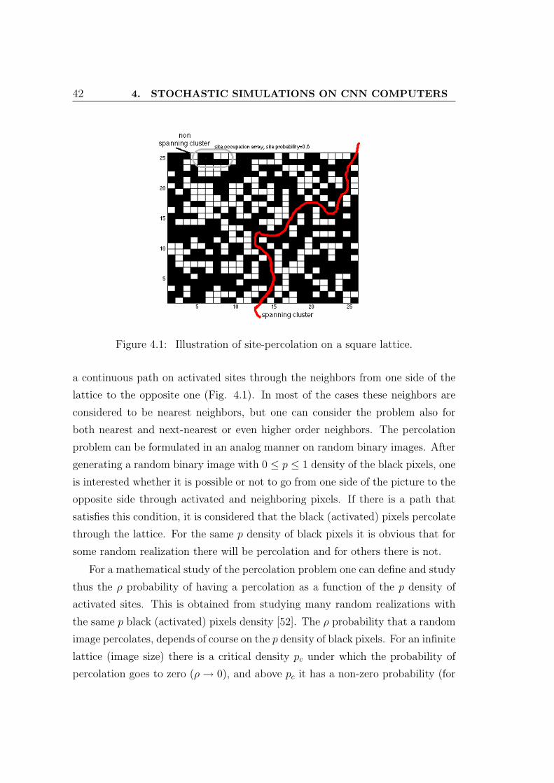
42 4. STOCHASTIC SIMULATIONS ON CNN COMPUTERS
Figure 4.1: Illustration of site-percolation on a square lattice.
a continuous path on activated sites through the neighbors from one side of the
lattice to the opposite one (Fig. 4.1). In most of the cases these neighbors are
considered to be nearest neighbors, but one can consider the problem also for
both nearest and next-nearest or even higher order neighbors. The percolation
problem can be formulated in an analog manner on random binary images. After
generating a random binary image with 0 ≤ p ≤ 1 density of the black pixels, one
is interested whether it is possible or not to go from one side of the picture to the
opposite side through activated and neighboring pixels. If there is a path that
satisfies this condition, it is considered that the black (activated) pixels percolate
through the lattice. For the same p density of black pixels it is obvious that for
some random realization there will be percolation and for others there is not.
For a mathematical study of the percolation problem one can define and study
thus the ρ probability of having a percolation as a function of the p density of
activated sites. This is obtained from studying many random realizations with
the same p black (activated) pixels density [52]. The ρ probability that a random
image percolates, depends of course on the p density of black pixels. For an infinite
lattice (image size) there is a critical density pc under which the probability of
percolation goes to zero (ρ → 0), and above pc it has a non-zero probability (for

4.3 The site-percolation problem 43
Figure 4.2: The probability of percolation, ρ in function of the density of activatedsites, p, in case of site-percolation with 4 neighbors, performed on systems withdifferent lattice sizes.
p → 1 we get of course always ρ → 1). In the thermodynamic limit (infinite
system size) we have a clear geometrical phase transition-like phenomena. For a
finite system the abrupt change for ρ(p) in the vicinity of pc is much smoother
(see Fig. 4.2).
There are several important quantities that are in general studied for this
phase-transition. The main quantities under investigation are some critical ex-
ponents, the shape of the ρ(p) curve and the value of pc. In the simple nearest-
neighbor case and for the two-dimensional case the site-percolation problem is
analytically solvable. For more complicated cases and for higher dimensionality
there are many available analytic approximation methods, but the most com-
monly used study method is Monte Carlo simulation.
4.3.2 The CNN algorithm
Here we will show how it is possible to determine the shape of the ρ(p) curve
on a fixed-size lattice by stochastic computer simulations on the CNN-UM. We
study the simple site-percolation problem on binary images. For percolation we
consider both the 4 nearest and 4 next-nearest neighbors (on CNN called the first
neighborhood of the cell: N1). From the architecture of the ACE16K CNN-UM
chip it results that a square lattice is used, each pixel having 8 other neighbors.
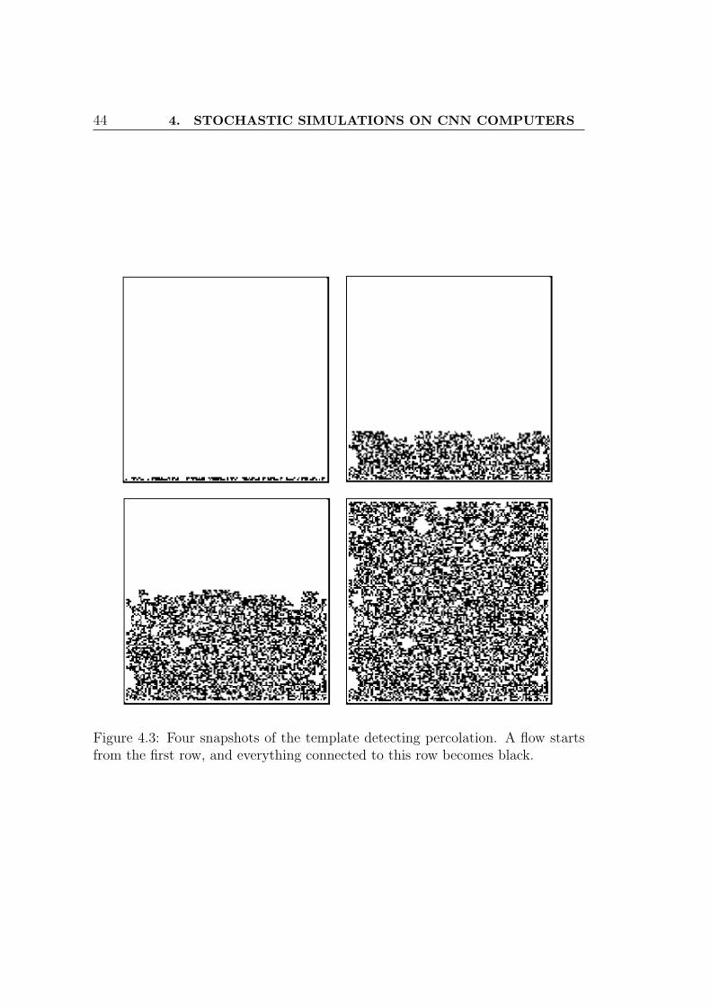
44 4. STOCHASTIC SIMULATIONS ON CNN COMPUTERS
Figure 4.3: Four snapshots of the template detecting percolation. A flow startsfrom the first row, and everything connected to this row becomes black.
4.3 The site-percolation problem 45
For determining the pc critical density and the ρ(p) curve one has to find the
percolation probability for many different densities of the black pixels. Finding
the complicated connected path through neighboring black pixels takes only one
single operation on the CNN chip. We are using a template, called figure recall,
presented also in Chapter 2, with parameters:
A =
0.5 0.5 0.50.5 4 0.50.5 0.5 0.5
,B =
0 0 00 4 00 0 0
, z = 3.
On CNN-UM chips the wiring allows us to consider 8 neighbors for each cell.
For solving the site-percolation with 4 nearest neighbors the template would be:
A = 0, 0.5, 0, 0.5, 4, 0.5, 0, 0.5, 0,B = 0, 0, 0, 0, 4, 0, 0, 0, 0,z = 1.
The input picture of the template will be the actual random image and the
initial state will contain only the first row of the image. Analyzing the template
one can easily realize that pixels, which have an input value equal to 1 (are
black), and have at least one neighbor with state value 1, will become black. In
this manner a flow starts from the first row making black all pixels, which were
black on the input picture and are connected through (the 8) neighbors to the
first row (Fig. 4.3). If on the output black pixels will remain in the last row, then
percolation exists. This simple template is a function in the image processing
library of the Bi-i v2 [39, 24]. Applying thus this template on many random
images generated through the methods presented in the previous section, it is
possible to study the classical site-percolation problem.
We also have to mention that this algorithm could be further generalized using
space-variant templates in which the connection parameters can be separately
defined for each cell. With this kind of CNN templates the bond-percolation and
directed percolation would be solvable in a very similar manner.
4.3.3 Numerical results
Numerical results were obtained on the same ACE16k [23] CNN chip, included
in the Bi-i v2 [24], which was used for the random number generator presented in
the previous chapter (Chapter 3). Results for the ρ(p) curve obtained on this chip
are plotted with circles on Fig. 4.4. On the same graph with square symbols it is
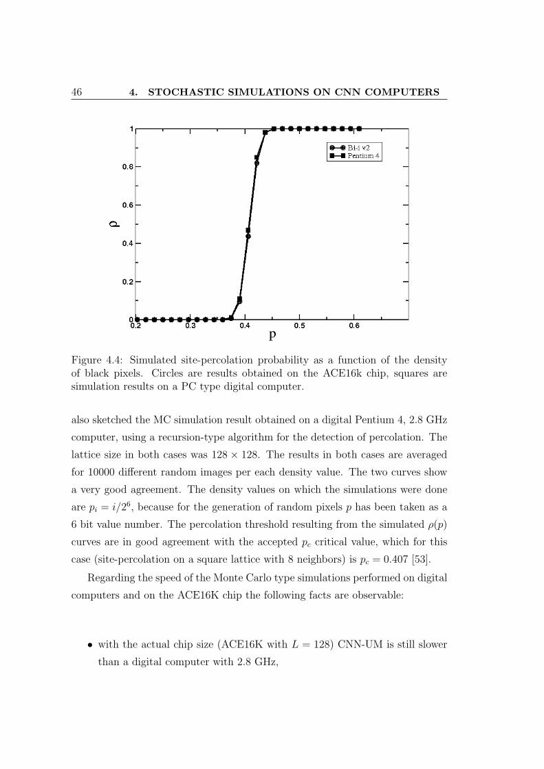
46 4. STOCHASTIC SIMULATIONS ON CNN COMPUTERS
Figure 4.4: Simulated site-percolation probability as a function of the densityof black pixels. Circles are results obtained on the ACE16k chip, squares aresimulation results on a PC type digital computer.
also sketched the MC simulation result obtained on a digital Pentium 4, 2.8 GHz
computer, using a recursion-type algorithm for the detection of percolation. The
lattice size in both cases was 128 × 128. The results in both cases are averaged
for 10000 different random images per each density value. The two curves show
a very good agreement. The density values on which the simulations were done
are pi = i/26, because for the generation of random pixels p has been taken as a
6 bit value number. The percolation threshold resulting from the simulated ρ(p)
curves are in good agreement with the accepted pc critical value, which for this
case (site-percolation on a square lattice with 8 neighbors) is pc = 0.407 [53].
Regarding the speed of the Monte Carlo type simulations performed on digital
computers and on the ACE16K chip the following facts are observable:
• with the actual chip size (ACE16K with L = 128) CNN-UM is still slower
than a digital computer with 2.8 GHz,

4.3 The site-percolation problem 47
Figure 4.5: Time needed for detecting percolation on 1000 images as a functionof the image linear size. Circles are results obtained on an ACE16k CNN-UMand squares are simulation results on a Pentium 4, 2.8GHz PC.
• on CNN-UM the time needed for detecting percolation grows linearly with
the linear size of the respective image, while on digital computers it scales
with the square of the lattice linear size.
Increasing thus the size of the chip will definitely favor the CNN-UM architecture
for such Monte Carlo type simulations on lattices. This trend results clearly from
Fig. 4.5, where on a log-log scale the simulation times are compared on digital
and CNN computers for different lattice (chip) sizes. It also worth mentioning,
that in the site-percolation problem mainly binary images are used, the state of
the system being saved in local logic memories (LLM). The ACE16K chip [23] was
developed mainly for image processing on analog images and the number of LLMs
is only two. This inconvenience effects considerably an optimized implementation
of the algorithm since many extra data transfer (converting to LAMs) has to be
done. On the other hand, the new Q-Eye chip [25] has 8 LAMs and 7 LLMs,
hence the running time would be considerably smaller. We also have to mention
that other type of architectures, like the asynchronous cellular processor array

48 4. STOCHASTIC SIMULATIONS ON CNN COMPUTERS
developed by Dudek [54], could show a speed-up of orders of magnitudes for this
algorithm.
4.4 The Ising model
As a second example for stochastic simulations, widely used in statistical physics,
we now consider the well-known two-dimensional Ising model [55]. Implementing
an MC study for this model on the CNN-UM is however not trivial. As it will be
argued later a straightforward application of the usual Glauber [56] or Metropolis
[57] algorithms could lead to unexpected problems due to the completely parallel
architecture of the CNN dynamics.
4.4.1 A brief presentation of the Ising model
The classical two-dimensional Ising model is the basic model for understanding
the paramagnetic-ferromagnetic second order phase-transition in magnetic sys-
tems [55]. The elements of the model are scalar spins with two possible states
σ = ±1. The spins are located on the sites of a lattice, and interact through
an exchange interaction with their neighbors. The strength of the interaction is
characterized by a J coupling constant. In the classical version of the model,
the interaction is only with nearest-neighbors and the interaction favors spins to
align in the same direction (J > 0). Without an additional magnetic field the
Hamiltonian of the system can be written as:
H = −J∑<i,j>
σiσj, (4.1)
< i, j > representing nearest neighbors.
If the system is in contact with a heat-bath there are thus two competing
effects acting on this spin ensemble. The entropic effect of the temperature,
that tends to disorder the orientation of the spins, and the ordering effect of the
exchange coupling. In two or higher dimension there is an order-disorder second
order phase-transition at a Tc > 0 critical temperature. This is visible in the
sharp variation of the order parameter r =< M > /N =< σ > in the vicinity of
Tc. The two-dimensional case is exactly solvable, although the analytic solution

4.4 The Ising model 49
is very complicated. For three dimensional lattices there is presently no exact
solution known. Beside of many analytical approximation methods, Monte Carlo
type studies present a basic tool for studying the Ising model in two and higher
dimensions.
There are many different MC type methods for studying this basic lattice
model. Most of them like the Metropolis [57] or the Glauber [56] algorithm are
of serial nature, meaning that in each step we update one single spin. In the
Metropolis algorithm [57] for example in each step we randomly choose a spin,
we calculate what would be the energy difference ∆E if that spin would be flipped.
• if ∆E ≤ 0 the spin will be flipped
• if ∆E > 0 the spin will be flipped with probability exp(−∆E/kT ).
Here we will implement a parallel version of the Metropolis algorithm, but it worth
mentioning that cluster algorithms, like the one proposed by Swendsen and Wang
[58] or Wolff [59], seem to be also appropriate for the parallel architecture of the
CNN-UM.
4.4.2 A parallel algorithm
Our goal was to implement the Metropolis algorithm [57] on the CNN Univer-
sal Machine. Working however parallel with all spins, creates some unexpected
problems due to the fact that nearest neighbors are updated simultaneously.
Imagine for instance an initial state where the spin-values (black and white,
correspondingly 1 and −1) are assigned using a chessboard pattern. Let us con-
sider now the Metropolis algorithm. On the chessboard pattern the state of a spin
is always the opposite of the state of the 4 nearest neighbors, so according to the
algorithm each spin will change its state. If all spins are updated simultaneously,
then the system will continuously switch between the two opposite chessboard
patterns. So for example at low temperatures, contrary to what is expected, this
system will not order in a simple ferromagnetic phase. In simulations we do not
start from a chessboard pattern, but this kind of patterns can randomly appear
in small regions of the system, and in case of a totally parallel algorithm they
do not disappear, causing unrealistic results. We could show other examples too,

50 4. STOCHASTIC SIMULATIONS ON CNN COMPUTERS
Figure 4.6: The chessboard mask used in our parallel algorithm.
different kind of patterns that cause unrealistic results in case of a totally parallel
update. The general problem is that the new state of each cell (spin) depends
on the state of the 4 nearest neighbors, so we should always avoid updating the
first-neighbors simultaneously.
For eliminating the parallel update of the nearest neighbors which causes such
problems, and still taking advantage of the parallel nature of the computer, we
decided to update the whole system in two consecutive steps. We impose an extra
chessboard mask on the system, and in each odd (even) step we update in a par-
allel manner the spins corresponding to the black (white) cells of the chessboard
mask. For the chosen spins the probabilities of changing the state are calculated
according to the simple Metropolis algorithm. This way nearest neighbors are
not updated simultaneously, and no unrealistic patterns are observed.
For giving a more detailed explanation why this method is basically equivalent
with the classical serial Metropolis dynamics, let us consider the two spins marked
with a and b on the chessboard pattern on fig. 4.6. On fig. 4.6 the white and
black pixels represent the mask used in our algorithm, the state of the spins can
be arbitrary. The energies, and thus the Metropolis probabilities of spins a and b
depend only on their 4 nearest neighbors, all of them marked with black on our
mask. If the states of all spins marked with black are fixed, then updating first
the spin a and then spin b, gives the same result as updating them at the same
time. This is true for all spins marked with white on the mask. If the states of

4.4 The Ising model 51
spins marked with black remain fixed, than it is totally equivalent that the spins
marked with white are updated simultaneously or in a well defined order (or even
in a random order with the condition that all of them are updated once). The
inverse can be proved in a similar manner: if the states of the spins marked with
white are fixed, we can update the black spins at one time-step, the result will be
equivalent with the result obtained after a serial update. So we can conclude, that
updating the whole system in two consecutive steps, using the chessboard mask,
the algorithm is equivalent with the serial Metropolis algorithm in which the spins
would be updated in a well-defined order. Detailed balance and ergodicity still
remains valid, so the obtained statistics should be the right one.
Implementing the above scheme on the CNN-UM is realized as follows (Fig.
4.7). In each step we have to build three additional masks:
• the first, N1, marks the spins with 4 similar neighbors (∆E = 8J),
• the second, N2, marks the spins with 3 similar neighbors (∆E = 4J),
• and the third, N3, represents all the other spins for which ∆E ≤ 0.
Separating these cells is relatively easy using logic operations and some tem-
plates which can shift the images in different directions (for ex. shifting to
East (or right) can be realized by the template: A = 0, 0, 0, 0, 2, 0, 0, 0, 0,B = 0, 0, 0, 1, 0, 0, 0, 0, 0, z = 0). The steps necessary for building these masks
(Fig. 4.7) could be briefly summarized as following:
• we build 4 images I1, I2, I3, I4 corresponding to the 4 directions (North,
West, South and East), which mark the spins (pixels) having a similar
neighbor in the given direction. This is realized always by shifting the
original image, representing the present state of the spin system, 1 step in
the opposite direction (if we want to check the Eastern neighbors we have to
shift the image to West), and performing exclusive-or operation between the
original and the shifted image (Note: on the Q-Eye chip the shift operator
is already an elementary instruction).
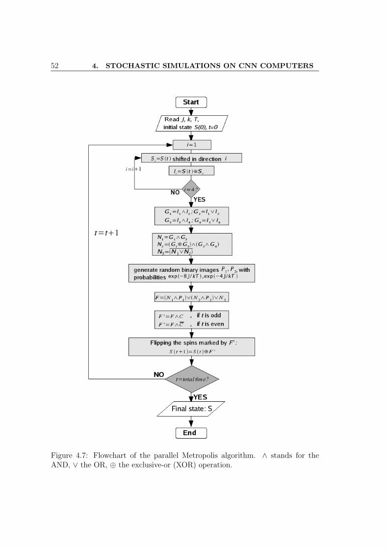
52 4. STOCHASTIC SIMULATIONS ON CNN COMPUTERS
Figure 4.7: Flowchart of the parallel Metropolis algorithm. ∧ stands for theAND, ∨ the OR, ⊕ the exclusive-or (XOR) operation.
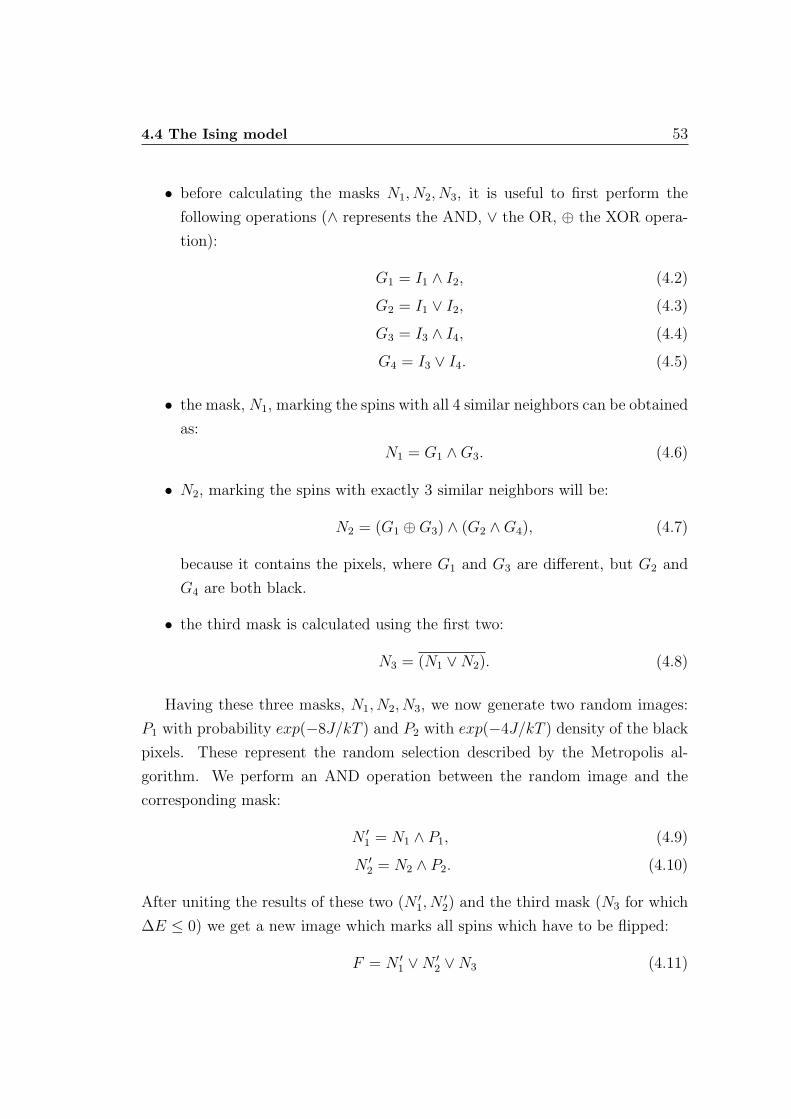
4.4 The Ising model 53
• before calculating the masks N1, N2, N3, it is useful to first perform the
following operations (∧ represents the AND, ∨ the OR, ⊕ the XOR opera-
tion):
G1 = I1 ∧ I2, (4.2)
G2 = I1 ∨ I2, (4.3)
G3 = I3 ∧ I4, (4.4)
G4 = I3 ∨ I4. (4.5)
• the mask, N1, marking the spins with all 4 similar neighbors can be obtained
as:
N1 = G1 ∧G3. (4.6)
• N2, marking the spins with exactly 3 similar neighbors will be:
N2 = (G1 ⊕G3) ∧ (G2 ∧G4), (4.7)
because it contains the pixels, where G1 and G3 are different, but G2 and
G4 are both black.
• the third mask is calculated using the first two:
N3 = (N1 ∨N2). (4.8)
Having these three masks, N1, N2, N3, we now generate two random images:
P1 with probability exp(−8J/kT ) and P2 with exp(−4J/kT ) density of the black
pixels. These represent the random selection described by the Metropolis al-
gorithm. We perform an AND operation between the random image and the
corresponding mask:
N ′1 = N1 ∧ P1, (4.9)
N ′2 = N2 ∧ P2. (4.10)
After uniting the results of these two (N ′1, N
′2) and the third mask (N3 for which
∆E ≤ 0) we get a new image which marks all spins which have to be flipped:
F = N ′1 ∨N ′
2 ∨N3 (4.11)

54 4. STOCHASTIC SIMULATIONS ON CNN COMPUTERS
Finally we use the chessboard mask, C, and allow only those spins to flip which
correspond to black (white) pixels if the time-step is odd (even).
F ′ = F ∧ C, if t is odd (4.12)
F ′ = F ∧ C , if t is even. (4.13)
Now F ′ marks all the spins which have to be flipped in this Monte Carlo step. The
flipping can be performed with a simple exclusive-or operation, and we obtain
the new state of the spin system:
S(t + 1) = S(t)⊕ F ′ (4.14)
During the algorithm the magnetization and energy can also be calculated.
The total magnetization of the system is equal with the difference between the
number of spins with positive and negative magnetization. We can use the Area
function included in the image processing library of the Bi-i [39], for counting the
number of black pixels on S(t). If this, representing the number of positive spins,
is denoted by m+, the magnetization of the system will be:
M = m+ − (L2 −m+) = 2m+ − L2, (4.15)
where L is the lattice size. For calculating the energy the Area function has to be
used on the I1, I2, I3, I4 images. The results (let us denote them as e1, e2, e3, e4)
will give us how many pixels have their bonds (in the respective direction) satis-
fied. Of course each bond appears twice in the total sum, so the energy will be:
E = −1
2(e1 + e2 + e3 + e4) + 2L2. (4.16)
This algorithm can be easily generalized for diluted Ising models [60], extra
masks marking the missing sites or bonds should be introduced. Also, in case of
CNN computers with more layers of cells, the three dimensional version of the
model could be studied in a similar manner.

4.4 The Ising model 55
Figure 4.8: Snapshots of the simulations performed on the ACE16k chip, fortemperature values T = 2, 2.3, 2.6, after t = 50, 250, 500 Monte Carlo steps.

56 4. STOCHASTIC SIMULATIONS ON CNN COMPUTERS
4.4.3 Numerical results
The simulations were performed again on the ACE16k chip with lattice size 128×128 [23]. The interaction constant is taken to be J = 1, and the value of the
Boltzmann factor is taken as k = 1 in the simulations (this changes only the
measuring units of the temperature). Fixed (1 - black) boundary conditions
were imposed. Some snapshots of the simulations can be seen on Fig. 4.8.
The spin system after t = 50, 250, 500 MC steps is presented at three different
temperatures T = 2, 2.3, 2.6. We can see that at the first temperature value
(T = 2) ferromagnetic order appears fast, at T = 2.3 (T being close to the critical
value) the order appears much slower, and at the last temperature (T = 2.6) we
are in the paramagnetic phase, where no spanning clusters are formed.
Simulation results obtained with the Metropolis type algorithms are sketched
on Figures 4.9, 4.10, 4.11. On these figure we compare the results of:
• the classical Metropolis algorithm on a digital computer (empty squares),
• the results of our parallel algorithm simulated on a digital computer (gray
triangles)
• and the results obtained on the ACE16K chip (black circles).
As mentioned in the previous chapter, the magnetization and the energy can be
easily calculated in each step of the algorithm, so the averages (< M >, < M2 >,
< E >,< E2 >) were calculated for 10000 Monte Carlo steps using a 1000
transient steps. By plotting the average magnetization, < M(T ) > (Fig. 4.9),
the specific heat, Cv(T ) (Fig. 4.10) and the magnetic susceptibility, χ(T ) (Fig.
4.11) as a function of the temperature one can conclude that different results are
in good agreement with each other. The specific heat, Cv, is the measure of the
heat energy required to increase the temperature of a unit quantity of a substance
by a certain temperature interval. The magnetic susceptibility, χ, is the degree
of magnetization of a material in response to an applied magnetic field. For these
Ising type spin systems the two quantities can be calculated in function of the
average magnetization and average energy of the system, measured during a long
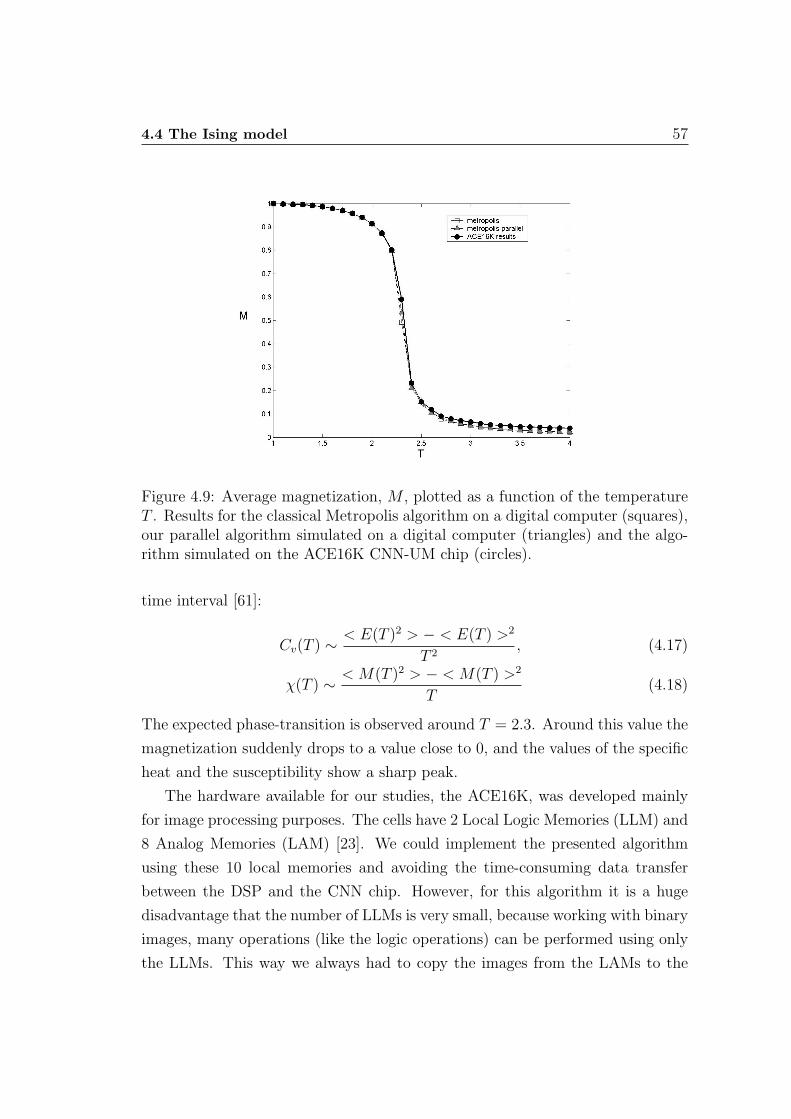
4.4 The Ising model 57
Figure 4.9: Average magnetization, M , plotted as a function of the temperatureT . Results for the classical Metropolis algorithm on a digital computer (squares),our parallel algorithm simulated on a digital computer (triangles) and the algo-rithm simulated on the ACE16K CNN-UM chip (circles).
time interval [61]:
Cv(T ) ∼ < E(T )2 > − < E(T ) >2
T 2, (4.17)
χ(T ) ∼ < M(T )2 > − < M(T ) >2
T(4.18)
The expected phase-transition is observed around T = 2.3. Around this value the
magnetization suddenly drops to a value close to 0, and the values of the specific
heat and the susceptibility show a sharp peak.
The hardware available for our studies, the ACE16K, was developed mainly
for image processing purposes. The cells have 2 Local Logic Memories (LLM) and
8 Analog Memories (LAM) [23]. We could implement the presented algorithm
using these 10 local memories and avoiding the time-consuming data transfer
between the DSP and the CNN chip. However, for this algorithm it is a huge
disadvantage that the number of LLMs is very small, because working with binary
images, many operations (like the logic operations) can be performed using only
the LLMs. This way we always had to copy the images from the LAMs to the

58 4. STOCHASTIC SIMULATIONS ON CNN COMPUTERS
Figure 4.10: Average specific heat, Cv, plotted as a function of the temperature T .Results for the classical Metropolis algorithm on a digital computer (squares), ourparallel algorithm simulated on a digital computer (triangles) and the algorithmsimulated on the ACE16K CNN-UM chip (circles).
Figure 4.11: Average susceptibility ,χ, plotted as a function of the temperature T .Results for the classical Metropolis algorithm on a digital computer (squares), ourparallel algorithm simulated on a digital computer (triangles) and the algorithmsimulated on the ACE16K CNN-UM chip (circles).
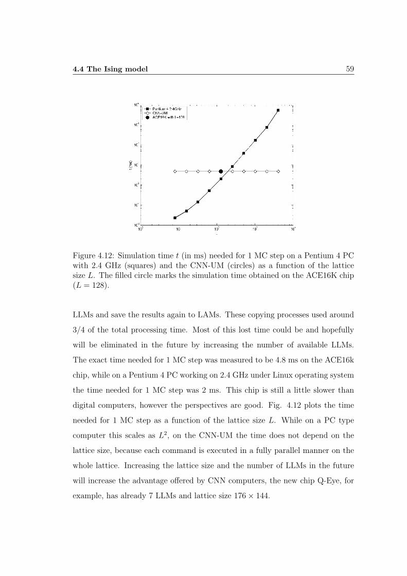
4.4 The Ising model 59
Figure 4.12: Simulation time t (in ms) needed for 1 MC step on a Pentium 4 PCwith 2.4 GHz (squares) and the CNN-UM (circles) as a function of the latticesize L. The filled circle marks the simulation time obtained on the ACE16K chip(L = 128).
LLMs and save the results again to LAMs. These copying processes used around
3/4 of the total processing time. Most of this lost time could be and hopefully
will be eliminated in the future by increasing the number of available LLMs.
The exact time needed for 1 MC step was measured to be 4.8 ms on the ACE16k
chip, while on a Pentium 4 PC working on 2.4 GHz under Linux operating system
the time needed for 1 MC step was 2 ms. This chip is still a little slower than
digital computers, however the perspectives are good. Fig. 4.12 plots the time
needed for 1 MC step as a function of the lattice size L. While on a PC type
computer this scales as L2, on the CNN-UM the time does not depend on the
lattice size, because each command is executed in a fully parallel manner on the
whole lattice. Increasing the lattice size and the number of LLMs in the future
will increase the advantage offered by CNN computers, the new chip Q-Eye, for
example, has already 7 LLMs and lattice size 176× 144.

60 4. STOCHASTIC SIMULATIONS ON CNN COMPUTERS
4.5 Discussion
The developed algorithms are suitable for the parallel structure of the CNN-
UM, however they mainly use binary operations, in case of which the ACE16k
chip does not show a profit as good as for analog wave-like operations. This
is another reason why the speed measured on the ACE16k is smaller than on
digital computers. As we discussed increasing the number of local memories and
lattice size could decrease the simulation time obtained on the ACE16k, but we
have to mention also that for these algorithms better architectures can be realized.
For example the asynchronous/synchronous cellular processor array developed by
Dudek [54], could show a speed-up of orders of magnitudes for these algorithms.
This kind of chip was not available for our experiments, the reason why we still
used the ACE16k, was to test the algorithms and show that they are possible to
implement.
Chapter 5
NP-hard optimization using aspace-variant CNN
In this Chapter CNN is used for NP-hard optimization. We prove, that a space-
variant CNN in which the parameters of all cells can be separately controlled,
is the analog correspondent of an Ising type (Edwards-Anderson [62]) spin-glass
system. Using the properties of CNN we show that one single operation using
our locally variant template, always yields a local minimum of the spin-glass
energy function. This way a very fast optimization method, similar to simulated
annealing, can be built. Estimating the simulation time needed for such NP-hard
optimization on CNN based computers, and comparing it with the time needed on
normal digital computers using the simulated annealing algorithm, the results are
very promising: CNN computers could be faster than digital computers already
at 10× 10 lattice sizes [3].
5.1 Motivations
Solving NP-hard problems is a key task when testing novel computing paradigms.
These complex problems frequently appear in physics, life sciences, biometrics,
logistics, database search, etc., and in most cases they are associated with impor-
tant practical applications as well [63]. The deficiency of solving these problems
in a reasonable amount of time is one of the most important limitation of digital
computers, thus all novel paradigms are tested in this sense. Quantum comput-
ing for example is theoretically well-suited for solving NP-hard problems, but the
61

62 5. NP-HARD OPTIMIZATION USING A SPACE-VARIANT CNN
technical realization of quantum computers seems to be quite hard. The advan-
tage of CNN-computing is that several practical realizations are already available
[22, 23, 24, 25]. The local control of the parameters of each cell, needed for our
algorithm is already partially realized on some hardwares (parameter z can be
locally controlled) and it is expected to be fully functional in the near future.
Beside the fundamental interest for solving NP hard problems, the importance
of this study consists also in motivating the development of hardwares in such
direction.
5.2 Spin-glass models
The aim of the present study is to prove that CNN computing is suitable for solv-
ing effectively complex optimization problems on spin-glass type lattice models.
Spin-glasses are disordered materials exhibiting a frustration in the optimal
magnetic ordering [62, 64]. The typical origin of this is the simultaneous presence
of competing interactions. The Ising-type spin-glass model [62] is a generalization
of the Ising model presented in Section 4.4.1. The elements of the model are scalar
spins with two possible states, σ = ±1, interacting through exchange interactions
with their neighbors. The coupling constants characterizing the interactions can
be different for each connection: Jij, and are randomly distributed in space. The
Hamiltonian of the system writes as
H = −∑<i,j>
Jijσiσj, (5.1)
< i, j > representing the neighbors. If external magnetic field is also applied:
H = −∑<i,j>
Jijσiσj −BN∑
i=1
σi. (5.2)
The energy landscape is complicated with many local minima. Finding the
ground-state is an NP-hard problem in many cases. Barahona [65] and Istrail
[66] has shown that the optimization of Ising type spin-glasses is an NP-hard
problem if and only if the spin system is defined on a non-planar lattice struc-
ture, meaning a lattice which can not be represented in two dimensions without

5.3 The CNN algorithm for optimization of spin-glass models 63
having crossing edges. In this study we will concentrate on the two-dimensional -
still non-planar - lattice structure, when the 4 nearest and 4 next-nearest neigh-
bors (the N1 CNN neighborhood with 8 neighbors) are considered (see fig. 2.1).
This lattice structure is most commonly used on CNN hardwares. We have to
mention here that CNN chips with more layers were also built (CACE1k), so our
optimization algorithm could be easily generalized for three-dimensional lattices
as well.
Besides its importance in condensed matter physics, spin glass theory has
in the time acquired a strongly interdisciplinary character, with applications to
neural network theory [67], computer science [63], theoretical biology [68], econo-
physics [69] etc. It has also been shown that using spin-glass models as error-
correcting codes, their cost-performance is excellent [70].
5.3 The CNN algorithm for optimization of spin-
glass models
We consider a two-dimensional CNN where the templates (parameters of Eq.
2.9) can be locally controlled. The Chua-Yang model is used and matrix A is
considered symmetric:
A(i, j; k, l) = A(k, l; i, j), A(i, j; i, j) = 1 for all (i, j). (5.3)
The elements are bounded
A(i, j; k, l) ∈ [−1, 1], (5.4)
where (i, j) and (k, l) denote two neighboring cells.
Matrix B, which controls the effect of the input image, will be taken simply
as:
B(i, j; i, j) = b and B(i, j; k, l) = 0, i, j 6= k, l. (5.5)
The parameter z is chosen as z = 0, so finally our template is defined by A, balone.
The state-equation of the system writes as
dxi,j(t)
dt= −xi,j(t) +
∑<k,l>∈N(i,j)
Ai,j;k,lyk,l(t) + bui,j, (5.6)

64 5. NP-HARD OPTIMIZATION USING A SPACE-VARIANT CNN
where xi,j is the state value, yi,j is the output, and ui,j is the input of the cell
(i, j) with neighborhood N(i, j) (8 neighbors and itself).
5.3.1 Relation between spin-glass models and CNN
In an earlier work Chua et al. [21] defined a Lyapunov function for the CNN,
which behaves like the ”energy” (Hamiltonian) of the system (see Section 2.2.2.1).
For the CNN defined above it can be written as
E(t) = −∑
<i,j;k,l>
Ai,j;k,lyi,jyk,l − b∑i,j
yi,jui,j, (5.7)
where < i, j; k, l > denotes pairs of neighbors, each pair taken only once in the
sum. yi,j denotes the output value of each cell and ui,j stands for an arbitrary
input image. By choosing the parameter b = 0, the energy of this special CNN
is similar with the energy of an Ising type system on square lattice with locally
varying coupling constants. The difference is that Ising spins are defined as
±1, while here we have continuous values between [−1, 1]. Since the A(i, j; k, l)
coupling constants can be positive and negative as well, locally coupled spin-
glasses can be mapped in such systems. In the following we will be especially
interested in the case when the A(i, j; k, l) couplings lead to a frustration and
the quenched disorder in the system is similar with that of spin-glass systems
([62, 64]).
As demonstrated by Chua et al. this Lyapunov function has two important
properties [21] (see theorems presented in Section 2.2.2.1):
1. it is always a monotone decreasing function in time, dE/dt ≤ 0, so starting
from an initial condition E can only decrease during the dynamics of the
CNN.
2. the final steady state is a local minimum of the energy: dE/dt = 0.
In addition to these, our CNN has also another important property: due to the
fact that A is symmetric and all self-interaction parameters are A(i, j; i, j) = 1,
the output values of the cells in a final steady state will be either 1 or −1, so
the local minima achieved by the CNN is an Ising-like configuration. This can

5.3 The CNN algorithm for optimization of spin-glass models 65
Figure 5.1: The DP plot of a cell. The derivative of the state value is presented infunction of the state value, for w(t) = 0 (continuous line) and w(t) > 0 (dashedline).
be understood by analyzing the driving-point (DP) plot of the system. The
derivative of the state value is plotted in function of the state value on fig. 5.1.
The state equation of a cell can be divided in two parts, one depending on the state
value of the cell, g(xi,j(t)), and the other part depending only on the neighbors:
dxi,j(t)
dt= g(xi,j(t)) + w(t), (5.8)
where
g(xi,j(t)) = −xi,j(t) + A(i, j; i, j) ∗ f(xi,j(t)), (5.9)
w(t) =∑
<k,l> 6=<i,j>
Ai,j;k,lyk,l(t) + bui,j. (5.10)
Because we have a coupled template in which w(t) changes in time, also the DP-
plot of the system changes in function of w(t) (on fig. 5.1 the case of w(t) = 0 is
plotted with a continuous line, and w(t) > 0 is represented with dashed line). We
can not predict the exact final steady state of the cell, but we can see that the
equilibrium points can not be in the (−1, 1) region, so the output of the cell will

66 5. NP-HARD OPTIMIZATION USING A SPACE-VARIANT CNN
be always ±1. The single exceptions will be the cells (spins) with 0 local energy,
in which case w(t) = 0. It can happen that these cells do not achieve a ±1 output
(although on real hardwares, in presence of real noise this is hardly probable),
but the state of these does not affect the energy of the Ising configuration. So
we can just randomly choose between −1 or 1. The result given by the CNN is
similar with finding more than one state at the same time.
We can conclude thus, that starting from any initial condition the final steady
state of the CNN using the presented template - meaning the result of an oper-
ation - will be always a local minimum of the spin-glass type Ising spin system
with local connections defined by matrix A. The fact that one single operation is
needed for finding a local minimum of the energy, gives us hope to develop fast
optimization algorithms.
5.3.2 The optimization algorithm
As already emphasized, the complex frustrated case (locally coupled spin-glass
type system), where the A coupling parameters generates a non-trivial quenched
disorder, will be considered here. The minimum energy configuration of such
systems is searched by an algorithm which is similar with the well-known sim-
ulated annealing method [48]. The noise is included with random input images
(ui,j values in eq. 5.7) acting as an external locally variable magnetic field. The
strength of this field is governed through parameter b. Whenever b is different
from zero, our CNN template minimizes the energy with form of eq. 5.7: the
first part of it being the energy of the considered spin-glass type model and the
second part an additional term, which gets minimal when the state of the system
is equal to the input image (the external magnetic field). If b is large, the result
will be the input image itself, if b = 0 the result is a local minimum of the pure
Ising-type system. For values in between, our result is a ”compromise” between
the two cases. Slowly decreasing the value of b will result in a process similar
with simulated annealing, where the temperature of the system is consecutively
lowered. First big fluctuations of the energy are allowed, and by decreasing this
we slowly drive the system to a low energy state. Since the method is a stochas-
tic one, we can of course never be totally sure that the global minimum will be

5.4 Simulation results 67
achieved, but good approximations can be obtained.
The steps of the algorithm are the following (see Fig. 5.2):
1. The A(i, j; k, l) template is initialized.
2. One starts from a random initial condition x, and b = b0.
3. A random binary input image u is generated with 1/2 probability of black
(1) pixels.
4. Using the x initial state and the u input image the CNN template is applied.
5. The value of b is decreased with steps ∆b.
6. Steps 3-5 are repeated until b = 0 is reached. The results of the previous
step (minimization) is considered always as the initial state for the next
step.
7. When reaching b = 0 the image (Ising spin configuration) is saved and the
energy is calculated.
Usually in simulated annealing many steps at a single temperature are needed.
Here the CNN template working in parallel replaces all these steps. We could
choose to run the given CNN template several times at a given value of b, but the
results would not improve. Instead of this we choose to repeat this whole cooling
process several times (denoted by n on Fig. 5.2). As a result of this process more
different final states will be achieved, and one gets higher probability to get the
right global minima.
5.4 Simulation results
In our studies spin-glass systems with connections A(i, j; k, l) = ±1 were simu-
lated. The p probability of the positive connections can be varied (influencing the
amount of frustration in the system) and we considered local interactions with
the first 8 nearest neighbors.
The simulation code was written in C, and the PDE system describing the
space-variant CNN was simulated using the 4th order Runge-Kutta method. The
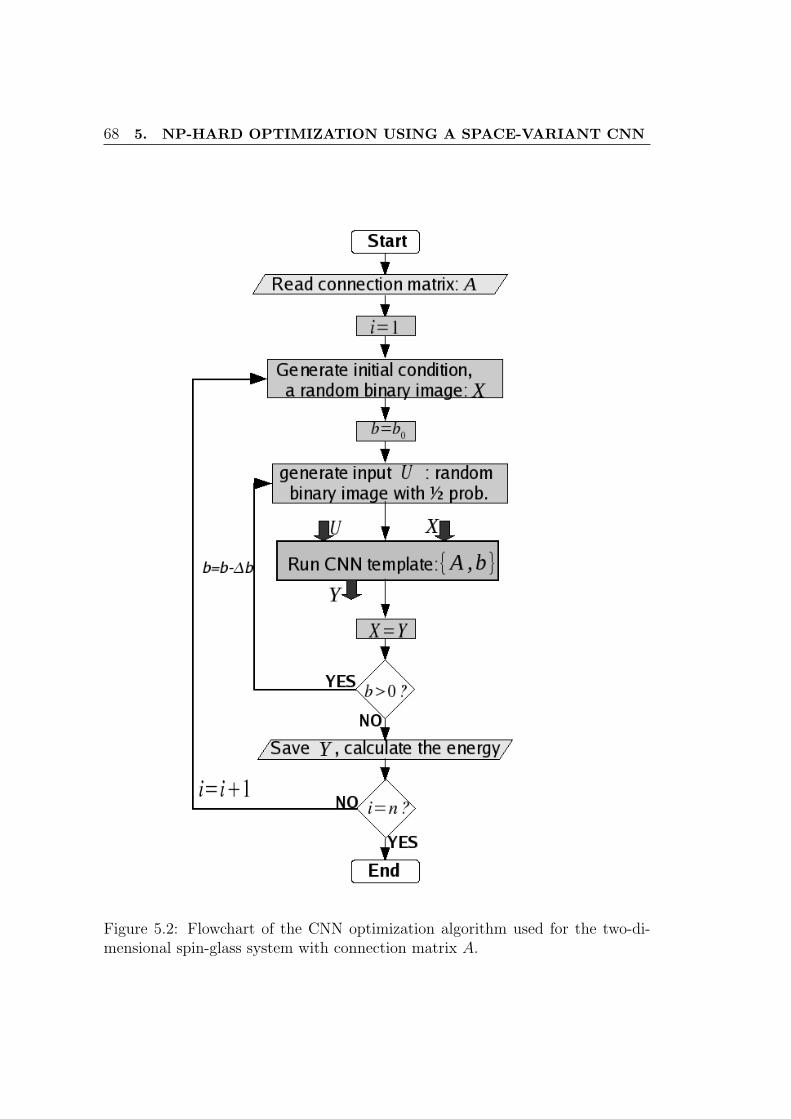
68 5. NP-HARD OPTIMIZATION USING A SPACE-VARIANT CNN
Figure 5.2: Flowchart of the CNN optimization algorithm used for the two-di-mensional spin-glass system with connection matrix A.

5.4 Simulation results 69
Figure 5.3: a) Number of steps needed to get the global minima as a function of∆b (system with 8× 8 cells). 4000 different systems were considered covering thewhole range of the possible p values. b) The optimal value of ∆b is shown as afunction of the lattice size L.
code was carefully tested with standard CNN templates. Writing this code was
necessary, because the CNN simulator of the Aladdin software is designed for
simulating the standard (space-invariant) CNN architecture, and also a very fast
code was needed, because in our method many CNN operations have to be simu-
lated, consuming a huge amount of processing time. This is also the reason why
our simulations were performed on relatively small system sizes, considering up
to 11× 11 cells.
For testing the algorithm and measuring the number of steps needed, we
previously have to search for the exact global minima. In case of small systems
with L = 5, 6 this search was quick and exact. For bigger systems the classical
simulated annealing was used with decreasing rate of the temperature T/Ti = 0.99
and performing 1000 Monte Carlo steps at each temperature.
The initial value of the noise level b0 must be carefully chosen. It has to
be large enough, in the beginning the result of the template must be almost
equivalent with the imposed input image, but choosing a high value also increases
the simulation time. Generally we can say, that at the starting of the template
(t = 0) in the state equation of the system (Eq. 5.6) the second part (representing
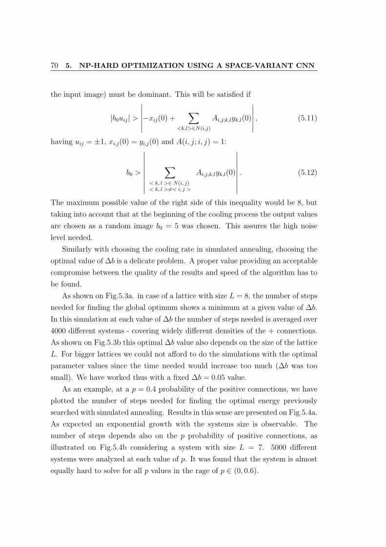
70 5. NP-HARD OPTIMIZATION USING A SPACE-VARIANT CNN
the input image) must be dominant. This will be satisfied if
|b0uij| >
∣∣∣∣∣∣−xij(0) +∑
<k,l>∈N(i,j)
Ai,j;k,lyk,l(0)
∣∣∣∣∣∣ , (5.11)
having uij = ±1, xi,j(0) = yi,j(0) and A(i, j; i, j) = 1:
b0 >
∣∣∣∣∣∣∣∣∣∑
< k, l >∈ N(i, j)< k, l > 6=< i, j >
Ai,j;k,lyk,l(0)
∣∣∣∣∣∣∣∣∣ . (5.12)
The maximum possible value of the right side of this inequality would be 8, but
taking into account that at the beginning of the cooling process the output values
are chosen as a random image b0 = 5 was chosen. This assures the high noise
level needed.
Similarly with choosing the cooling rate in simulated annealing, choosing the
optimal value of ∆b is a delicate problem. A proper value providing an acceptable
compromise between the quality of the results and speed of the algorithm has to
be found.
As shown on Fig.5.3a. in case of a lattice with size L = 8, the number of steps
needed for finding the global optimum shows a minimum at a given value of ∆b.
In this simulation at each value of ∆b the number of steps needed is averaged over
4000 different systems - covering widely different densities of the + connections.
As shown on Fig.5.3b this optimal ∆b value also depends on the size of the lattice
L. For bigger lattices we could not afford to do the simulations with the optimal
parameter values since the time needed would increase too much (∆b was too
small). We have worked thus with a fixed ∆b = 0.05 value.
As an example, at a p = 0.4 probability of the positive connections, we have
plotted the number of steps needed for finding the optimal energy previously
searched with simulated annealing. Results in this sense are presented on Fig.5.4a.
As expected an exponential growth with the systems size is observable. The
number of steps depends also on the p probability of positive connections, as
illustrated on Fig.5.4b considering a system with size L = 7. 5000 different
systems were analyzed at each value of p. It was found that the system is almost
equally hard to solve for all p values in the rage of p ∈ (0, 0.6).

5.5 Speed estimation 71
Figure 5.4: a) Number of steps needed to find the optimal energy as a functionof the lattice size L. The density of positive connections is fixed to p = 0.4,and parameter ∆b = 0.05 is used. b) Number of steps needed for getting thepresumed global minima as a function of the probability of positive connectionsp (system with size L = 7).
5.5 Speed estimation
Finally, let us have some thoughts about the estimated speed of such an opti-
mization algorithm. As mentioned earlier, on the nowadays available CNN chips,
only parameter z can be locally varied, parameters A and B are 3× 3 matrices,
uniformly applied for all cells (Chapter 2). The reason for no local control of
A and B seems to be simply the lack of motivations. In image processing ap-
plications no really useful algorithms were developed, which would require these
locally variable connections. Realizing the local control of A and B is technically
possible and is expected to be included in the newer versions of the CNN chips.
This modification would not change the properties and the speed of the chip, only
the control unit and template memories would become more complicated. Also,
introducing the templates on the chip would take a slightly longer time.
In the specific problem considered here the connection parameters have to be
introduced only once for each problem, so this would not effect in a detectable
manner the speed of calculations. Based on our previous experience with the
ACE16K chip (with sizes 128×128) [1, 2] we can make an estimation of the speed

72 5. NP-HARD OPTIMIZATION USING A SPACE-VARIANT CNN
Figure 5.5: a) Time needed to reach the minimum energy as a function of thelattice size L. Circles are estimates on CNN computers and stars are simulatedannealing results on a 3.4 GHz Pentium 4 PC. Results are averaged on 10000different configurations with p = 0.4 probability of positive bonds. For the CNNalgorithm ∆b = 0.05 was chosen. For simulated annealing the initial tempera-ture was T0 = 0.9, final temperature Tf = 0.2 and the decreasing rate of thetemperature was fixed as 0.99.
for the presented optimization algorithm. This chip with its parallel architecture
solves one template in a very short time - of the order of microseconds. For each
step in the algorithm one also needs to generate a random binary image. This
process is already 4 times faster on the ACE16K chip than on a 3.4 GHz Pentium
4 computer and needs around 100µs (see Chapter 3, [1]). It is also helpful for
the speed, that in the present algorithm it is not needed to save information at
each step, only once at the end of each cooling process. Saving an image takes
roughly 0.25 milliseconds on the ACE16K, but this is done only once after several
thousands of simulation steps. Making thus a rough estimate for our algorithm, a
chip with similar properties like the ACE16K should be able to compute between
1000− 5000 steps in one second, independently of the lattice size.
Using the lower estimation value (1000 steps /second) and following up the
number of steps needed in case of p = 0.4, the estimated average time for solving

5.5 Speed estimation 73
one problem is plotted as a function of the lattice size on Fig. 5.5 (circles).
Comparing this with the speed of simulated annealing (SA) performed on a 3.4
GHz Pentium 4 (squares on Fig. 5.5), the results for larger lattice sizes are clearly
in favor of the CNN chips.
For testing the speed of simulated annealing we used the following parameters:
initial temperature T0 = 0.9 , final temperature Tf = 0.2, decreasing rate of the
temperature 0.99. Results were averaged for 10000 different bond distributions.
The necessary number of Monte Carlo steps was always carefully measured by
performing many different simulations, using different number of Monte Carlo
steps, and comparing the obtained results. From Fig. 5.5 it results that the
estimated time needed for the presented algorithm on a CNN chip would be
smaller than simulated annealing already at 10× 10 lattice sizes.
There are many applications in which global minimum is not crucial to be
exactly found, the minimization is needed only with a margin of error. In such
cases the number of requested steps will decrease drastically. As an example in
such sense, it has been shown that using spin-glass models as error-correcting
codes, their cost-performance is excellent [70], and the systems are usually not
even in the spin-glass phase. In this manner by using the CNN chip, finding
acceptable results could be very fast, even on big lattices.
Chips with 2 and 3 layers of cells were also produced (see Table 2.1) and
increasing the number of layers is expected in the near future. This further
extends the number of possible applications. On two layers is possible to map
already a spin system with any connection matrix (even globally coupled spins)
and also other important NP-hard problems (e.g. K-SAT) may become solvable.


Chapter 6
Pulse-coupled oscillatorscommunicating with light pulses
In this Chapter a non-standard cellular nonlinear network is studied, built up
by pulse-coupled oscillators. The oscillators are communicating with light: they
are capable of emitting and detecting light-pulses, and in this way global cou-
pling can be achieved. Firing is always favored by darkness, so the interactions
are of inhibitory nature. Experimental and computational studies reveal that al-
though no direct driving force favoring synchronization is considered, for a given
interval of the firing threshold parameter, phase-locking appears. This weak syn-
chronization is sometimes accompanied by complex dynamical patterns in the
flashing sequence of the oscillators [4], [6] . Here we also present perspectives
of this ongoing work: how these simple oscillators are further developed, and
how they can be separately programmed. A cellular nonlinear network can be
defined using these new oscillators, allowing dynamical spatio-temporal input.
This shows many interesting applicabilities (like detection via phase-patterns or
synchronization).
6.1 Motivations
In information technology the accent is slowly shifting from the development of
single processors to developing systems with many interacting units. Nowadays,
a million 8-bit microprocessors can be placed on a single 45 nm CMOS chip,
the biggest supercomputer has a quarter million processors (the Blue Gene),
75
766. PULSE-COUPLED OSCILLATORS COMMUNICATING WITH
LIGHT PULSES
and the new cellular visual microprocessor chip (Q-Eye) contains 25k processors.
Moreover, physical parameters, like wire delay and power dissipation start to play
an important role in the algorithmic theory of computing [16]. The evolution of
these processing systems is still marked by the lack of proper algorithms. When
studying this kind of systems, our long-term question is what kind of useful
functions could be solved with these interacting units. We can not answer this
question thinking in the classical way: here we have the problem, how can we
solve it? We have to think inversely: this is the behavior of the system, we have
the type of solutions, so we should find the problem to solve, the basic function
of the system. For getting the answers, first the behavior of these systems must
be deeply understood.
In this longer project we were interested to study the behavior of a non-
standard CNN which differs from the standard model in two important features:
the type of coupling, and the number of connections. Trying to imitate the behav-
ior of real neurons we wanted to study pulse-coupled cells, and to achieve coupling
between a much larger neighborhood. We realized this with pulse-coupled oscil-
lators, communicating with light-pulses. We have to mention that our goal was
not to develop new kind of hardwares, the experiments help to understand the
behavior of these networks. Although, communication using light could be a use-
ful idea even in some hardware projects, because it resolves wiring problems, and
even global coupling can be achieved.
As the first part of this project we studied the collective behavior of quasi-
identical oscillators. Interesting synchronization phenomena was observed. The
results of this study will be presented in this Chapter. Our second goal was
to develop separately controllable oscillators: each oscillator having separately
programmed parameters and behavior. Using these units a cellular nonlinear
network model can be defined. Studying this non-standard CNN offers many
interesting possibilities. We will present the perspectives of this ongoing project
in the last section.

6.2 Introduction 77
6.2 Introduction
Synchronization of quasi-identical coupled oscillators is one of the oldest and
most fascinating problems in physics [71, 72, 73]. Its history goes back to C.
Huygens who first noticed the synchronization of pendulum clocks hanging on
the same wall. Besides mechanical or electric oscillator systems, nature is also
full with several amazing examples in this sense [74, 75, 76, 77]. Synchronization
in all these systems appears as a result of some specific coupling between the
units. This coupling can be local or global, and can be realized through a phase-
difference minimizing force [78, 79] or through the pulses emitted and detected
by the oscillators [80, 81]. In most of these synchronizing systems there is a
clear driving force favoring synchronization, and in such a way the appearance of
this collective behavior is somehow trivial. In this Chapter however, a nontrivial
synchronization will be presented. This weak synchronization (phase-locking)
appears as a by-product of a simple collective optimization rule.
One well-known phenomenon which inspired us in this work is the collective
behavior and synchronization of fireflies [82]. Although our aim here is not to
model fireflies, the oscillators (”electronic fireflies”) considered in our system are
somehow similar to them: they are capable of emitting light-pulses and detecting
the light-pulse of the others. In this sense our system is similar to an ensemble
of fireflies although the coupling between the units is different. From another
perspective, the oscillators behave like pulse-coupled ”integrate and fire” type
neurons [80, 81, 83]. Contrary to the classical integrate and fire oscillators, in
the considered system an inhibitory type global interaction is considered. This
means that the firing of one oscillator delays (and not advances) the phase of all
the others. This system does not necessarily favor synchronization, it is rather
designed to keep a desired W light intensity in the system. This light intensity is
controlled by a firing threshold parameter G imposed globally on the oscillators.
Surprisingly, as a by-product of this simple rule, for certain region of the firing
threshold parameter, phase-locking and complex patterns in the flashing sequence
of the oscillators will appear. We believe that such dynamical laws could be
realistic for many biological systems.

786. PULSE-COUPLED OSCILLATORS COMMUNICATING WITH
LIGHT PULSES
The studied system will be described in more details in the following section.
The used electronic device will be presented and the obtained non-trivial collec-
tive behavior will be studied. In order to get more confidence in the observed
non-trivial results computer simulations were also performed. The oscillators
were further developed, being now separately programmable, i.e. the parameters
(templates) and behavior of the cells can be space-variant. Some perspectives
offered by this ongoing project will be briefly presented in the last section.
6.3 The experimental setup
6.3.1 The cell and the interactions
The constructed units are similar to integrate and fire type oscillators [80] with
a modified interaction rule. Their coupling and communication is through light,
the units are capable of emitting and detecting light-pulses. The oscillators are
practically realized by a relatively simple circuit, the main elements being a pho-
toresistor and a Light Emitting Diode (LED). Each oscillator, i, has a character-
istic voltage Ui, which depends on the resistance, Ri, of its photoresistor. The
light intensity influences the value of Ri in the following sense: when the light
intensity increases Ri decreases, leading to a decrease in Ui. In the system there
is a global controllable parameter G, identical for all oscillators. By changing the
parameter G, one can control the average light intensity output, W , of the whole
system. If the voltage of the oscillator grows above this threshold (Ui > G) the
oscillator will fire, this meaning its LED will flash. This flash occurs only if a
minimal time period Tminihas elapsed since the last firing. The oscillator has also
a maximal period, meaning if no flash occurred in time Tmaxi, then the oscillator
will surely fire. In laymen terms firing is favored by darkness and the value of
the controllable G parameter characterizes the ”darkness level” at which firing
should occur. Through this simple rule the G parameter controls the average
light intensity output of the system.

6.3 The experimental setup 79
Figure 6.1: Experimental setup. The oscillators are placed on a circuit board,which can be placed inside a box with matt glass walls. From the circuit boardthe data is automatically transferred to the computer. A closer view of a singleoscillator is also shown.
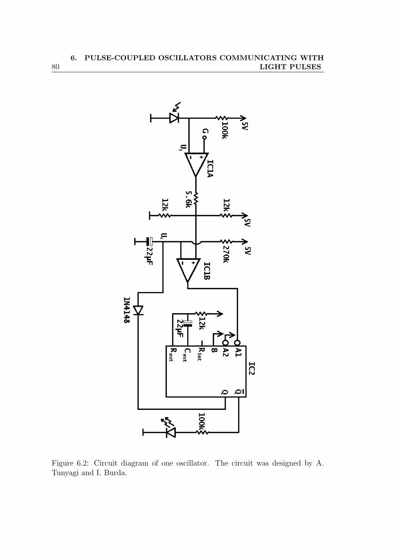
806. PULSE-COUPLED OSCILLATORS COMMUNICATING WITH
LIGHT PULSES
Figure 6.2: Circuit diagram of one oscillator. The circuit was designed by A.Tunyagi and I. Burda.

6.3 The experimental setup 81
6.3.2 The electronic circuit realization of the oscillators
The technical realization of the above dynamics is illustrated in Fig. 6.2. After
the system has fired the 22 µF capacitor is completely discharged (Uc = 0) by
the negative pulse from the inverted output of the monostable. As soon as the
light flash ended, the same capacitor will start charging from the current flow
through the 270 KΩ resistor. The IC1B comparator will trigger another flash as
soon as the potential on the mentioned capacitor, Uc, will overcome the value
fixed by the group of three resistors on its positive input. We could also say,
that this capacitor ”measures the time” (see Fig. 6.3), and the flashing period
is given by the group of the three resistors. This period can take two different
values Tmin or Tmax: two of the resistors are connected to constant potentials
(ground and +5 V), but the third resistor is connected to the output of the
second comparator IC1A which will have a value depending on the ratio between
the reference voltage (G firing threshold) and a certain amount of light measured
by the photo resistor. When the voltage, U , of the photo-resistor is smaller than
the firing threshold G, the flashing period determined by the three resistors will
be the minimal time-period Tmin (black curve on Fig. 6.3). When U > G, the
flashing period will be Tmax (gray curve on Fig. 6.3). This does not mean that
the time between two consecutive flashes can take only these two values. If Tmin
has already expired, and the light intensity suddenly decreases changing also the
voltage (and the time-period) imposed by the resistors, the flash will be induced
in that moment (dashed line on Fig. 6.3).
The flash time is determined by the second capacitor together with the 12
KΩ resistor connected to the monostable. The time of one flash is around 200
ms. The photoresistor has a relatively low reaction time around 40 ms, while
the minimal and maximal period of firing are around 800 ms and 2700 ms. Of
course these characteristic electronic parameters differ slightly (2− 10%) among
the units.
The oscillators are placed on a circuit board in the form of a square lattice
(see Figure 6.1). The maximal number of oscillators which can be included are
24. A computer interface and program controls the G threshold parameter and
allows us to get information automatically about the states of all oscillators. The

826. PULSE-COUPLED OSCILLATORS COMMUNICATING WITH
LIGHT PULSES
Figure 6.3: After a flash the capacitor starts to charge, Uc increasing in time.The new flash can appear only between Tmin and Tmax.
state of an oscillator is recorded as 0 if the oscillator does not emit light and 1
when the oscillator fires (emits light). Whenever the state of the oscillator system
changes, the program writes in a file the corresponding time with a precision of
milliseconds and the new states of the units.
To obtain an enhanced global interaction the whole system is placed inside
a closed box. The box has matt glass mirror walls to uniformly disperse the
light-pulses in the box.
6.4 Collective behavior
At constant light intensity each unit behaves as a simple stochastic oscillator.
Whenever the G threshold is under a given Gc value the oscillator will fire with
its minimal period and above Gc with its maximal period. Gc depends of course
on the imposed light intensity. Considering more oscillators (i = 1, . . . , n) and by
letting them interact, interesting collective behavior appears for a certain range
of the G threshold parameter.
Due to the inhibitory nature of the considered interaction, during the firing

6.4 Collective behavior 83
Figure 6.4: Four interacting oscillators placed on the circuit board.
846. PULSE-COUPLED OSCILLATORS COMMUNICATING WITH
LIGHT PULSES
of oscillator i the characteristic voltages of the others (Uj, j 6= i) will decrease. If
the G parameter is so small, that even under this condition the other oscillators
can still fire (Uj > G), than all oscillators will fire in an uncorrelated manner.
Each of them will be firing at its own Tminjperiod and the interaction is thus not
efficient. In such case no collective behavior can be observed.
Increasing the value of G will make the pulse-like interaction efficient. The os-
cillators will avoid firing simultaneously and a simple phase-locking phenomenon
appears. The pulse of one unit (let us assume i) delays the firing of the others
by decreasing their voltages below the threshold: Uj < G, j 6= i. Due to the tiny
differences in the coupling between the pairs (caused for example by different
distances) and in the parameters of the electronic elements, the Uj voltages are
different. The immediate consequence of this is that the next firing will occur
most probably in the oscillator with the highest voltage (counting of course only
those oscillators, which are already capable of firing). This oscillator is the one
which was influenced the less by the light-pulse of the previous firing. If the
total combined time of firing for the n oscillators is smaller than the period Tmax,
the result is that after very short time phase-locking appears, and a firing chain
(with period T ∈ [Tmin, Tmax]) will form, each oscillator firing in a well-defined
sequence. For a given system and a fixed G threshold this stable pattern is always
the same. If the total time of firing of the n oscillators exceeds Tmax, the firing
pattern will be much longer and more complex.
Increasing further and over a limit the G threshold parameter the previously
discussed weak synchronization (phase-locking) disappears. In this case the volt-
ages of all oscillators are much smaller than the threshold value Ui < G, so the
firing of a unit can not influence the others. All oscillators will fire with their
own Tmaxiperiod and no interesting collective behavior is observed. Again, the
interaction is not efficient.
6.4.1 Experimental results
The collective behavior of the system can be easily analyzed by plotting a kind of
phase-histogram for the oscillator ensemble. Choosing a reference oscillator, the

6.4 Collective behavior 85
relative phases of all the others are defined by measuring the time difference be-
tween their pulse and the last pulse emitted by the reference oscillator. Studying
these time-delays during a longer time period a histogram is constructed for their
distribution. This histogram shows how frequently a given time-delay occurred
and gives thus a hint whether a constant firing pattern is formed or not.
Experimental and computer simulated results for the phase-histogram confirm
the above presented scenario of the collective behavior. As an example, on Fig.
6.5,6.6, 6.7, 6.8 results obtained on a relatively small system with n = 5 oscillators
are shown for four different values of the G threshold parameter. Experimental
and simulation results are compared (we present the details of the simulations in
the next section).
For a small threshold parameter (G = 500 mV), no self-organization appears
(Fig. 6.5). Due to the fact that the characteristic time-periods of the oscillators
are slightly different, almost all values will occur with the same probability in the
phase-histogram. Starting with G = 1300 mV a kind of order begins to emerge,
and a trend towards the self-organization of the oscillator pulses is observed (e.g.
Fig. 6.6 for G = 2000 mV). In the neighborhood of G = 3000 mV threshold
value (Fig. 6.7) clear phase-locking appears. One can observe that a stable firing
pattern has formed, each oscillator has an almost exact phase relative to the
reference oscillator. For an even higher value (e.g. G = 4200 mV), disorder sets
in again, phase-locking disappears and all oscillators fire independently with their
own maximal period (Fig. 6.8).
6.4.2 Simulation results
In the second column of Fig. 6.5, 6.6, 6.7, 6.8 we present the corresponding
simulation results. In simulations the parameters of the oscillators are defined
as follows: the average minimal time period is Tmini= 900 ms, the average
maximal period Tmaxi= 2700 ms, and the average flashing time Tflash = 200
ms. For an easier comparison, the values are chosen to be similar with the
real experimental data. We considered a uniform distribution of the oscillators
parameter around these average values using a ±50 ms interval for Tmin and
Tmax and a ±20 ms interval for Tflash. One could argue of course that a Gaussian
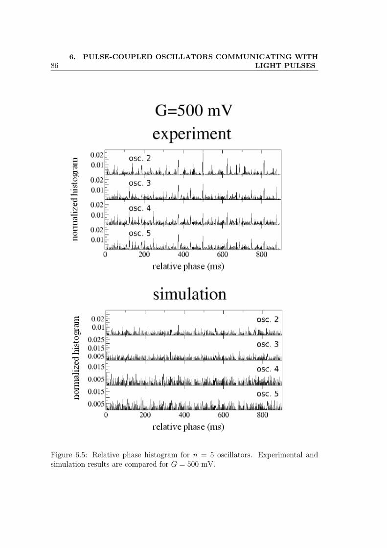
866. PULSE-COUPLED OSCILLATORS COMMUNICATING WITH
LIGHT PULSES
Figure 6.5: Relative phase histogram for n = 5 oscillators. Experimental andsimulation results are compared for G = 500 mV.

6.4 Collective behavior 87
Figure 6.6: Relative phase histogram for n = 5 oscillators. Experimental andsimulation results are compared for G = 2000 mV.
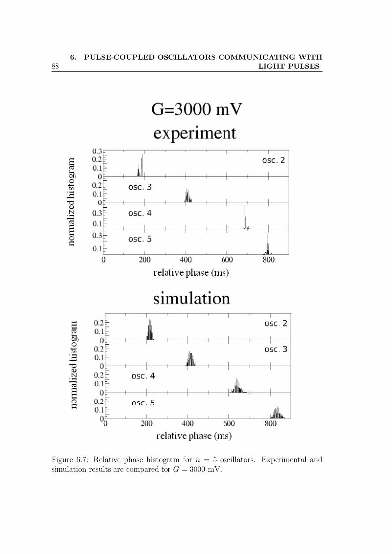
886. PULSE-COUPLED OSCILLATORS COMMUNICATING WITH
LIGHT PULSES
Figure 6.7: Relative phase histogram for n = 5 oscillators. Experimental andsimulation results are compared for G = 3000 mV.
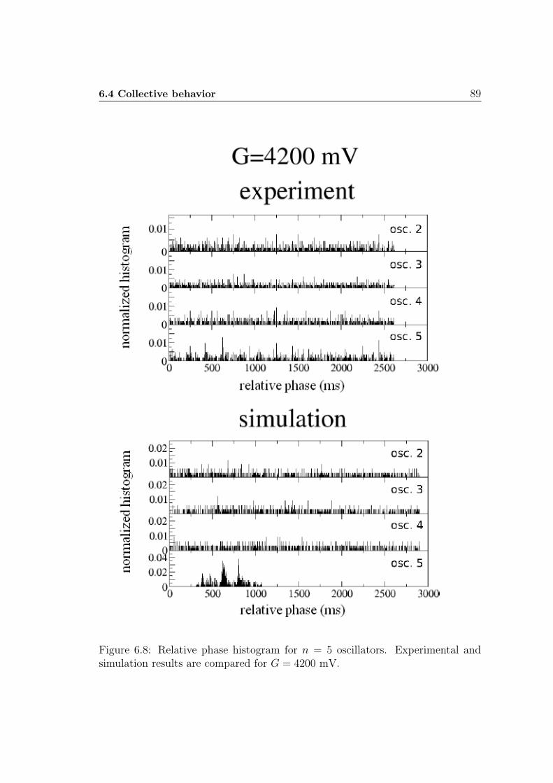
6.4 Collective behavior 89
Figure 6.8: Relative phase histogram for n = 5 oscillators. Experimental andsimulation results are compared for G = 4200 mV.

906. PULSE-COUPLED OSCILLATORS COMMUNICATING WITH
LIGHT PULSES
distribution would be much more appropriate, but given the fact that here we
simulate relatively small number of oscillators the exact statistics is irrelevant.
Considering some deviations from the average is however important in order to
reproduce the collective behavior of the system. An uncorrelated noise in time
is also considered. This will randomly shift the Tmin, Tmax and Tflash periods of
each oscillator at each cycle. Again, a uniform distribution on a ±20 ms interval
was considered.
The characteristic voltages of the oscillators are set to be in the interval 4100±100 mV in dark, 2100 ± 100 mV when one single LED is flashing and 1050 ±100 mV when two LEDs are flashing simultaneously. Whenever k LEDs are
simultaneously flashing the characteristic voltages of the others are considered to
be 2100/k ± 100 mV, however for n = 5 oscillators only very rarely happens to
have more than two oscillators simultaneously firing. These values were chosen
to approximately match the experimental ones, and we do not try to give a
theoretical model for the nonlinear behavior of the photoresistor. Fluctuations in
time and among the parameters of the oscillators are again included. Differences
in the strength of the coupling between pairs of oscillators are however neglected.
Using these parameters, it is assumed that each oscillator can flash whenever its
voltage exceeds the threshold G. The flashing cannot occur earlier than Tminior
later than Tmaxirelatively to its last firing.
On Fig. 6.5, 6.6, 6.7, 6.8 the simulated phase-histograms of the oscillators are
plotted and compared with the corresponding experimental data. The observed
experimental results, including the non-trivial synchronization (phase-locking),
were successfully reproduced.
6.4.3 The order parameter
It is also possible to define a kind of order-parameter that characterizes the ob-
served synchronization level. There are several methods for measuring the order
in a synchronizing system (like measuring the entropy of the phase-histogram),
but almost any of the methods fails when increasing the size of the system. The
reason is that very long, complex patterns appear, and the histogram is compli-
cated even when the system is synchronized and shows a clear pattern. Finally
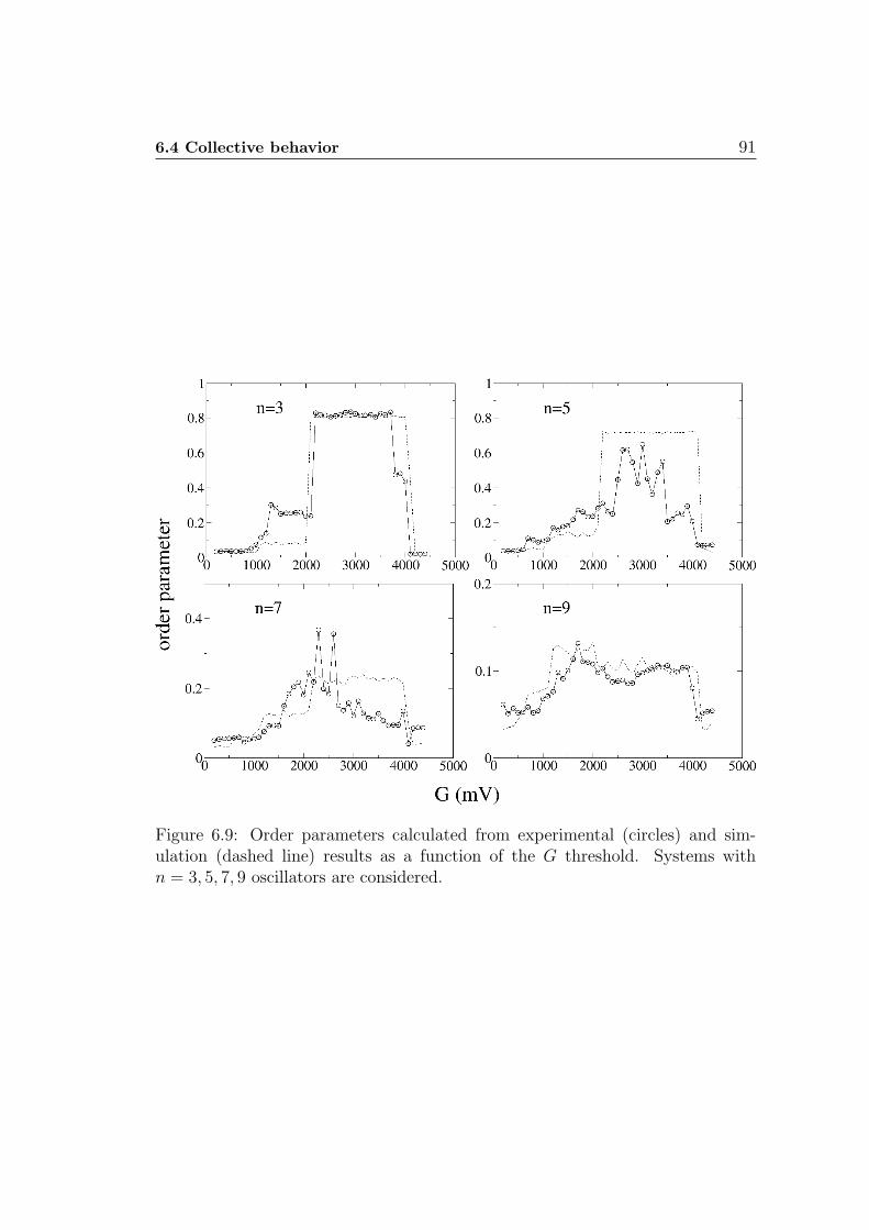
6.4 Collective behavior 91
Figure 6.9: Order parameters calculated from experimental (circles) and sim-ulation (dashed line) results as a function of the G threshold. Systems withn = 3, 5, 7, 9 oscillators are considered.

926. PULSE-COUPLED OSCILLATORS COMMUNICATING WITH
LIGHT PULSES
we used a heuristic method. This order parameter also decreases when increasing
the size of the system, still it was the most acceptable method.
The order parameter is calculated as following :
1. A reference oscillator k is chosen and the phases of all oscillators are calcu-
lated relative to this oscillator.
2. Let hi(τ) denote the value of the normalized phase-histogram for oscillator
i (i = 1, . . . , n, i 6= k) corresponding to phase difference (time difference)
value τ . Since we have a normalized histogram, hi(τ) ∈ [0, 1] gives the
occurrence probability of phase difference value τ during the measurement
(∑
f hi(τ) = 1).
3. Smoothing is performed on the phase-histogram. A window of width a is
defined (we have chosen a = 30 ms); shifting the window with ∆τ = 1 ms
step, for each discretized value of τ the sum:
Hi(τ) =
τ+a/2∑j=τ−a/2
hi(j) (6.1)
is calculated for each oscillator i.
4. Let rk denote the difference between the maximum and minimum value of
Hi(τ) averaged over all oscillators:
rk =1
n− 1
n∑i=1,(i6=k)
max(Hi)−min(Hi). (6.2)
5. Items 1-4 are repeated considering each oscillator in the system as reference
oscillator.
6. Finally, an averaging is performed over all the obtained rk values (k =
1, . . . , n). The final order parameter is calculated thus as:
r =
∑nk=1 rk
n. (6.3)
Averaging as a function of the reference oscillator is beneficial in order to
get a smoother curve when only partial phase locking is detected (Figure

6.5 Perspectives 93
6.6.). In such cases the phase-diagrams are very sensible on the choice of
the reference oscillator.
A short motivation of this algorithm is that, using parameter r our goal is to
detect if the phase-histograms of the oscillators are showing high peaks, or if the
values are grouped in certain regions of the phase-space.
On Fig. 6.9 the r order parameter is plotted as a function of the G threshold
value. Systems with n = 3, 5, 7 and 9 oscillators are considered. Experimental
(circles) and simulation results (dashed line) are again in good agreement. The
figure also illustrates that for an intermediate G interval value phase-locking
appears. This weak synchronization is better (r is bigger) when there are less
units in the system. One obvious reason for this is that by increasing n the total
time of firing of the oscillators will increase and slowly exceed the value Tmax.
As a result of this the firing pattern will change from a simple ”firing chain” to
a much longer and more complicated pattern, decreasing the value of the order
parameter.
From Fig. 6.9 it is also observable that the experimental results show more
intensive fluctuations. The reason for this is probably the complex noise present
in the system.
6.5 Perspectives
A system of electronic oscillators communicating through light-pulses was studied.
The oscillators have identical behavior and quasi-identical parameters. The units
were designed to optimize the average light intensity of the emitted light-pulses,
and no direct driving force favoring synchronization was considered. Although our
experiments focused on relatively small systems (up to 24 oscillators) interesting
and rich collective behavior was observed. As a nontrivial result it was found
that the inhibitory coupling induced a partial phase-locking for a certain interval
of the controllable threshold parameter [4].
Our further goal in this ongoing project was to develop separately controllable
oscillators. Using these units a new kind of CNN model can be defined, in which
the state value of each oscillator is the measured light intensity. The study of

946. PULSE-COUPLED OSCILLATORS COMMUNICATING WITH
LIGHT PULSES
these networks is still under way, here we only present some perspectives of this
project.
6.5.1 Separately programmable oscillators
The oscillators were further developed, so our units are already separately pro-
grammable. The following parameters can be programmed in each unit:
• Tmin, the minimal period
• Tmax, the maximal period
• Tflash, flashing time
• A, the light intensity of the flash
• G, the firing threshold
The local and global dependency control (the behavior) of the oscillators can
be also separately defined with a short C-like program introduced in each oscil-
lator. The number of possibilities is huge. The oscillators can be set to fire when
the measured light intensity exceeds the threshold value G, this way the type of
interactions will become exhibitory; or similarly to the interactions presented in
the first part of this Chapter, we can define inhibitory type interactions, when
firing is favored by darkness. We can also introduce a time-delay before the fir-
ing, imitating somehow the delays introduced by the synapses in neural networks.
Another important benefit is that we can also program these oscillators to change
some of the parameters during the experiment.
6.5.2 Cellular nonlinear networks using pulse-coupled os-cillators
Placing the oscillators on a square lattice, the whole system can be described as
a non-standard cellular nonlinear network in which the state value of a cell (an
oscillator), xij, is the measured light intensity
xi,j(t) =∑
<k,l> 6=<i,j>
Ak,lyk,l(t−∆) +∑
<k,l>
uk,l(t−∆) + z, (6.4)

6.5 Perspectives 95
where Ak,l are the flashing light intensities of the neighbors; the output yk,l, is
1 when firing, and 0 otherwise; ∆ is the time-delay introduced, or a kind of
reaction-time of the cell; uk,l is the input, which can be a local light intensity
imposed from outside; and z is the global light intensity level characterizing
the environment. The size of the interacting neighborhood (< k, l >) can be
approximately controlled by changing the G threshold parameters or the A light
intensities. As mentioned already the behavior of the oscillators can be set in
many different ways, defining the firing conditions, or more exactly the output
function, yk,l.
This non-standard CNN has many benefits:
• the size of the interacting neighborhood can be large, even global coupling
can be achieved
• dynamical, time-dependent input can be introduced
• we can easily program the cells to have a certain reaction time, time-delay
∆
• it is also possible to change some parameters (like ∆, A or G) as a function
of the dynamics
There is however an important disadvantage as well: we can not control the
connections individually (we do not have A(i, j; k, l)), the firing of one cell will
be detected by all interacting neighbors.
As further goals during this project we mention:
• Studies on the role of the reaction time, ∆, in the interactions. When ∆ = 0,
exhibitory interactions tend to synchronize the cells, inhibitory interactions
cause phase-delays between the interacting neighbors, and phase-locking
appears: complex patterns are formed and the phase-portrait will get sta-
bilized. Preliminary simulations show, that changing the ∆ parameter,
inhibitory connections can cause synchronization and exhibitory interac-
tions will show phase-locking. So the type of interactions and the value of
the reaction time are strongly correlated. The detailed study of the effects
caused by the reaction time is important, because even if we do not have

966. PULSE-COUPLED OSCILLATORS COMMUNICATING WITH
LIGHT PULSES
separable connections with each neighbor, this time-delay somehow imitates
the delays caused by synapses in neural networks.
• Another important study would be to dynamically change the parameters in
function of the behavior, or the input. For example, if the reaction times of
the cells get smaller at each firing caused by a strong input, than repeating
the input pattern a couple of times, we can teach the system. The next
time the same input is started, the involved cells will react and fire much
earlier than the other cells, ”predicting what they expect, based on their
previous experience”.
• Detecting different spatio-temporal events with the observed phase-patterns
or synchronization phenomena is another promising application area.
Studying the behavior of programmable interacting units is important because
in information technology Moore’s law is expected to be continued by increasing
the number of processor cores. The algorithms for effectively coordinating the
units are still missing. Beside the interesting behavior found in a system of quasi-
identical oscillators, this project offers further interesting possibilities for deeply
understanding the behavior of this kind of systems.

Chapter 7
Conclusions
The results presented in this dissertation show that the CNN-UM can be ef-
ficiently used for many different applications in physics as well. The non-de-
terministic random number generator presented in Chapter 3 can be useful for
many different algorithms (also in image processing), and its speed shows already
advantages relative to digital computers [1]. Here, we used this RNG for im-
plementing stochastic simulations on the CNN-UM. It was shown that detecting
percolation can be solved with one single template on the CNN-UM, and also a
parallel version of the Monte Carlo method for the two-dimensional Ising model
can be effectively implemented [2] [5] (Chapter 4).
Chapter 5 further motivates the development of these hardwares, proving
that a space-variant CNN could be used for optimization of spin-glass systems.
Spin-glass models have a strongly interdisciplinary character and as a basic NP-
hard problem their importance goes far beyond condensed matter physics. Our
results show that the proposed NP-hard optimization method could be very fast
on CNN-UM hardwares [3].
The goal of this interdisciplinary study was not only to use CNN computing
in physics, but also to use physics-motivated studies for the further development
of computing. In the last chapter of this thesis we studied the physical properties
and collective behavior of a cellular nonlinear network built up by pulse-coupled
oscillators communicating with light [6]. This ongoing project shows interesting
perspectives from the viewpoint of CNN computing as well.
97

Summary
7.1 Methods
In the course of my work theoretical methods, computer simulations
and experiments were harmonically combined.
The theory of Cellular Nonlinear/Neural Networks , including the
theorems demonstrated by Chua et. al. [21], were used for finding the
appropriate algorithms and templates, and demonstrating the analogy
between CNN and spin-glass type systems. Statistical physics and
well-known stochastic simulation methods were also used.
From a methodical point of view, the development of the realistic
random number generator is original because the physical phenom-
ena (thermal noise of the hardware) is successfully combined with a
chaotic cellular automaton. The random number generator and also
the other stochastic algorithms developed for the CNN based archi-
tecture, were first tested using the CNN simulator of the Aladdin
software [38]. The programs were written in Analogic Macro Code
(AMC). After successful testing with simulations the programs were
directed to the Bi-i v2 camera computer [24], which contains a DSP
and an ACE16K CNN chip with 128× 128 cells. Time measurements
were also made on this chip.
When simulating a locally variant CNN, I was obliged to renounce on
the CNN simulator of the Aladdin software, in which the templates
can not be separately controlled for each cell. I also needed a very

7.2 New scientific results 99
fast simulation method, because the NP-hard optimization of spin-
glasses was a time-consuming simulation. Finally I wrote the simula-
tion of my locally variant CNN in C, using the 4th order Runge-Kutta
method for the simulation of the PDE’s. After carefully testing my
program with well-known templates, I could use it for simulating the
considered NP-hard optimization method. The results obtained with
the new method were also compared with results given by the classical
simulated annealing. This program was also written in C.
The experimental setup for the non-conventional CNN composed of
oscillators communicating with light, was developed by Arthur Tun-
yagi and Ioan Burda [6]. They built a system very suitable for ex-
periments. Beside an interactive program in which parameters of the
system could be changed, measurements could be also made in an
easy manner, the states of all oscillators were written out in files in
function of time. These data-files could then be easily analyzed with
Matlab or C.
7.2 New scientific results
Thesis ]1: Generating non-deterministic sequences of true random
binary images on the CNN-UM, using a chaotic cellular automaton
perturbed with the natural noise of the CNN-UM chip [1] [5].
For successfully implementing stochastic simulations the crucial start-
ing point is a good random number generator (RNG). Taking advan-
tage on the fact that the CNN-UM chip is a partially analog device,
I used its natural noise for generating ”realistic” random numbers,
more precisely non-deterministic sequences of random binary images.
This assures an important advantage relative to digital computers,
especially for Monte Carlo type simulations. The natural noise of the
CNN-UM chip is usually highly correlated in space and time, so it can

100 7. CONCLUSIONS
not be used directly to obtain random binary images. My method is
based thus on a chaotic cellular automaton perturbed with the nat-
ural noise of the chip after each time step. Due to the used chaotic
cellular automaton, generated by appropriate CNN templates, the
correlations in the noise will not induce correlations in the generated
random arrays. Moreover, the real randomness of the noise will kill
the deterministic properties of the chaotic cellular automaton [1].
1.1. I developed an algorithm based on a chaotic cellular
automaton perturbed with the natural noise of the CNN-
UM chip, generating random binary images with equal (1/2)
probability of the black and white pixels.
I used one of the pseudo-random number generators already devel-
oped on the CNN-UM [31, 40] called the PNP2D. This is a chaotic
cellular automaton (CA), relatively simple and fast, which passed all
important RNG tests and shows very small correlations, so it is a
good candidate for a pseudo-random number generator. It generates
binary values, 0 (white) and 1 (black), with the same 1/2 probability
independently of the starting condition.
In my algorithm after each time step the result of the chaotic CA is
perturbed with a noisy binary image (array) (using exclusive-or oper-
ation). The noisy image is simply obtained by using a threshold CNN
template on a uniform gray-scale image with value a, at a threshold
value of a+ z. This way in each cell showing a noise level higher than
z, the value of the random image will be changed. This perturbation
is usually very small, and due to its nature it will not change the
good statistics of the CA, as I also proved it by correlation tests (see
Chapter 2) [1]. Although the deterministic property of the CA will be
lost, two random sequences starting from the same initial condition
will become different quickly.

7.2 New scientific results 101
My experiments were made on the ACE16K chip with 128× 128 size
in the Bi-i v2 camera computer. Time measurements show that with
this size of the chip, the time needed for generating one random binary
value is roughly 7 ns. On a Pentium 4, 2.8 GHz machine, generating
only pseudo-random values, this time is approximately 33 ns. We
can see thus that, beside the advantage offered by the analog device,
parallel processing makes CNN-UM also faster [1].
1.2. I constructed an algorithm which can generate ran-
dom binary images with any probability, p, of the black pixels
using more images with probability 1/2, generated with the
previous algorithm.
When using the RNG for implementing stochastic simulations, it is
very important that one should be able to generate images with any
probability of the black pixels. I solved this problem by construct-
ing an algorithm which combines n images with 1/2 probability of
the black pixels P1, . . . , Pn (generated with the previous algorithm).
From these images we then construct n independent images I1, . . . , In
(without overlapping: Ii AND Ij = ∅ for any i 6= j), each of them
with pi = 1/2i probability of the black pixels. Using this set any
image with a probability p, represented on n bits, can be constructed
(for details see Chapter 3) [1].
Thesis ]2: Developing CNN-UM algorithms for Monte Carlo type
simulations of some classical problems of statistical physics and im-
plementing them on the CNN Universal Machine [1, 2].
Once a properly working RNG is available on the CNN-UM, it is
possible to implement Monte Carlo (MC) type simulations for two-
dimensional lattice-type models. Generating random initial condi-
tions for cellular automata models is straightforward, and many sim-

102 7. CONCLUSIONS
ple stochastic lattice models can be relatively easily solved. I have cho-
sen two well-known problems of statistical physics: the site-percolation
problem [49, 52] and the two dimensional Ising model [55]. Both of
them opens a huge class of problems, and in many cases my algo-
rithms can be easily modified for studying more special cases related
to these models. For both of the algorithms the previously developed
RNG, the parallel structure of the CNN, special CNN templates and
the analog-and-logic nature of the implementation plays an important
role.
2.1. I showed that it is possible to detect site-percolation
on a binary image, using one single CNN template, called
”figure recall”; I developed and tested the algorithm on the
ACE16K chip included in the Bi-i v2 camera computer [1]
[5].
I used the CNN template often called as ”figure recall” template (in-
cluded also in the image processing library of the Bi-i v2 [39]) to
efficiently detect site-percolation on a binary random image. The in-
put picture of the template is the actual random binary image, and
the initial state will contain only the first row of the image. For per-
colation, both nearest and next-nearest neighbors (or the N1 CNN
neighbors) are considered. The template values are chosen in a way
that pixels which have an input value equal to 1 (are black), and have
at least one neighbor with state value 1, will become black. In this
manner a flow starts from the first row making black all the pixels
which were black on the input picture, and are connected through
neighbors to the first row. If on the final output will remain black
pixels in the last row, then percolation exists.
I tested this simple algorithm on many different binary images, with
different probabilities of black pixels. The probability of having per-
colation in function of the probability of the black pixels, shows a

7.2 New scientific results 103
phase-transition at p = 0.407 density of black pixels [53]. Results ob-
tained on the ACE16K chip are in good agreement with results given
by MC simulation results obtained on a digital Pentium 4, 2.8GHz
computer, using a recursion-type algorithm for detecting percolation.
2.2. I implemented the two-dimensional Ising model on
the ACE16K chip by modifying the Metropolis algorithm to
fit the parallel structure of the CNN [2] [7].
There are many Monte Carlo type algorithms used for simulating
the Ising model, but most of them are of serial nature. I modified
one of the most known algorithms, the Metropolis algorithm [57],
to fit the parallel structure of the CNN-UM. In this algorithm first
I used simple CNN templates like shifting and logic operations, for
building the masks marking the spins with different energy. Accord-
ing to the Metropolis algorithm, the spins will be flipped in each
Monte Carlo step with different probabilities depending on their en-
ergy: p = exp(−∆E/kT ), if ∆E > 0 and p = 1 if ∆E ≤ 0. For
randomly selecting the spins which will be flipped in each step we
use the random number generator, previously presented. The totally
parallel updating process causes some unexpected problems: because
the flipping probability is always calculated based on the states of
the 4 nearest neighbors (defining the energy of the given spin), we
have to avoid flipping the nearest neighbors simultaneously. It may
cause the appearance of unrealistic patterns (for more explanations
see Chapter 4). For avoiding the problems caused by the total parallel
update I introduced an additional (chessboard type) mask and allow
only those spins to flip which correspond to black (white) pixels if the
time-step is odd (even) (for details see Chapter 4). This way nearest
neighbors can never be flipped simultaneously, but the parallel nature
of the algorithm is still partially preserved: each Monte Carlo step is
realized with two consecutive steps. [2, 3].
104 7. CONCLUSIONS
I implemented the algorithm on the ACE16K chip (lattice size 128×128) in the Bi-i v2, and also tested the algorithm simulating it on dig-
ital computer in C, and comparing the results of simulations and ex-
periments with the results given by the classical Metropolis algorithm.
The results are in good agreement. Time measurements performed on
the ACE16k chip are also promising [2, 3].
Thesis ]3: NP-hard optimization of frustrated, two-dimensional spin-
glass systems, using locally variant CNN templates [3] [8].
I have shown that using a CNN-UM in which the connections (and re-
spective template parameters) can differ from cell to cell, it is possible
to study a huge variety of complex problems. NP-hard optimization
would be one of the promising applications of this kind of hardwares
[63]. I simulated a locally variant CNN and developed an algorithm
for optimization of frustrated spin-glass systems.
3.1. I demonstrated that a CNN with locally variant con-
nections is the analog correspondent of a spin-glass system:
all local energy minimas are equivalent.
I used a CNN in which the A parameters are locally defined: A(i, j; k, l) ∈[−1, 1], where (i, j) and (k, l) mark two neighbor cells. I also consid-
ered centrally symmetric connections: A(i, j; k, l) = A(k, l; i, j) and
A(i, j; i, j) = 1 for all (i, j); the parameters B which control the ef-
fect of the input image will be taken simply as: B(i, j; i, j) = b and
B(i, j; k, l) = 0; z = 0. Based on the theorems demonstrated by Chua
et al. [21], I proved that the Lyapunov function defined for this CNN
is equivalent with the energy of a spin-glass system [62, 64] where
the connection matrix is described by parameters A. The only dif-
ference between the two systems is that in the CNN we have analog
values and not discrete ones(±1) like usually in the spin systems. I
also proved that the local energy minimum states of the two systems

7.2 New scientific results 105
coincide, so the result of the CNN template will always yield a local
energy minimum of the spin-glass system.
3.2. I constructed a CNN algorithm based on principles
similar with simulated annealing. This finds the global op-
timum of frustrated spin-glass systems with a good approx-
imation and promising speed.
Using the properties demonstrated in the previous subthesis, I built
a CNN algorithm for finding the optimal state of two-dimensional
spin-glass systems. The algorithm is based on principles similar with
simulated annealing [48]. Noise is introduced with input images, the
role of temperature is taken by parameter b, which is slowly decreased
during the algorithm. I tested the algorithm with simulations, mea-
suring the steps needed for an acceptable error rate. Estimations on
the speed of the algorithm are very promising (see chapter 5) [3] .
Thesis ]4: Weak synchronization phenomena observed in a non-
standard CNN built from globally coupled, biologically inspired, elec-
tronic oscillators which are communicating with light pulses [6].
I studied a simple system composed of biologically inspired, electronic
oscillators, capable of emitting and detecting light-pulses. The con-
structed units are integrate and fire type oscillators [80] with a mod-
ified (inhibitory type) interaction rule: their behavior is designed for
keeping a desired light intensity, W , in the system. Each oscillator has
a characteristic voltage, Ui, which decreases as the global light inten-
sity grows. There is a global controllable parameter G in the system,
identical for all oscillators. If the voltage of an oscillator grows above
this threshold (Ui > G) the oscillator will fire, this meaning its LED
will flash. This flash occurs only if a minimal time period Tminihas
elapsed since the last firing. The oscillator has also a maximal pe-
106 7. CONCLUSIONS
riod, meaning if no flash occurred in time Tmaxi, then the oscillator
will surely fire. In laymen terms firing is favored by darkness and
the value of the controllable G parameter characterizes the ”darkness
level” at which firing should occur. Through this simple rule the G
parameter controls the average light intensity output of the system.
Experimental and computational studies reveal that although no driv-
ing force favoring synchronization is considered, for a given interval of
W , a weak form of synchronization, phase-locking, appears [6]. The
goal of this ongoing project is to develop a programmable system
where the oscillators can be separately controlled. Placing these os-
cillators on a square lattice, the whole system can be described as a
non-standard cellular nonlinear network in which the state value of a
cell (an oscillator) is the measured light intensity. Studying the behav-
ior of this non-standard CNN could reveal interesting synchronization
phenomena, which could be used as basic, programmable functions in
such kind of systems.
7.3 Application of the results
The application possibilities resulting from Thesis 1 come straightfor-
ward. Generating random numbers on the CNN-UM is important not
only in statistical physics, as proved in Thesis 2. Random sequences
and stochastic algorithms are also common in other areas as well (im-
age processing [84, 85], process control, games, numerical calculations
etc.). Pseudo-randomness and a repeatable random number series is
sometimes helpful. It makes easier the debugging of the codes and can
be a necessary condition for implementing specific algorithms. It also
carries some limitations. Since it is deterministic and results from a
chaotic update rule, for many initial conditions it might have finite
repetition periods. The fact that the natural noise of the analog CNN-
UM chip can be used to generate non-deterministic sequences is an

7.3 Application of the results 107
important advantage relative to digital computers. This can be useful
in Monte Carlo type simulations, when solving complicated statistical
physics problems with large ensemble averages, as discussed in Thesis
2.
Although the algorithms presented in Thesis 2 were developed for
two classical models of statistical physics, we feel that as the CNN-
UM is further developed in the future they could be used with suc-
cess for several similar problems. The methods presented here are
important because they give a CNN-compatible algorithm for study-
ing the proposed problems. I have shown that the recursive type
algorithm for detecting site-percolation can be replaced by one single
CNN template, and Monte Carlo type algorithms (in this case the
Metropolis algorithm) can be modified to fit the parallel architecture
of the CNN-UM. The two problems discussed here represent a whole
class of problems in statistical physics, many of these still intensely
studied in the present days. In case the CNN-UM chips are further
developed (for example using locally variable templates, like discussed
in Thesis 3) these algorithms could be easily modified to implement
bond-percolation, directed percolation, diluted Ising models, etc. [50].
The algorithm presented in Thesis 3 could be tested only with sim-
ulations. I believe however that it can be used for many important
applications. Solving NP-hard problems is a key task when testing
novel computing paradigms. These complex problems are associated
with life sciences, biometrics, logistics, parametric database search,
wireless communications, etc. [63]. The deficiency of solving these
problems in a reasonable amount of time is one of the most important
shortcomings of digital computers, thus all novel paradigms are tested
in this sense. As shown in Thesis 3, CNN computing shows good per-
spectives for such kind of problems, and this should also motivate the
further development of CNN chips in the indicated direction. The
specific NP-hard optimization problem studied here has also many
applications. Besides its importance in condensed matter physics,

108 7. CONCLUSIONS
spin glass theory has in the time acquired a strongly interdisciplinary
character, with applications to neural network theory [67], computer
science [63], theoretical biology [68], econophysics [69] etc. It has also
been shown that using spin-glass models as error-correcting codes,
their cost-performance is excellent [70], and the systems usually are
not even in the spin-glass phase. In this manner finding acceptable
results could be very fast even on big lattices considering the parallel
architecture of the CNN.
Thesis 4, being the first part of a longer project, is much more the-
oretical. It contributes in understanding the collective behavior of
a system of electronic oscillators. The system is interesting because
the considered integrate-and-fire type oscillators are communicating
with light, thus global coupling can be achieved. Although the in-
hibitory type interactions do not necessarily favor synchronization,
phase-locking is observed. Our goal is to further develop the system,
separately controlling the parameters of all oscillators. By placing the
oscillators on a square lattice, the whole system can be described as
a non-standard cellular nonlinear network in which the state value
of a cell (an oscillator) is the measured light intensity. Studying the
behavior of this non-standard CNN could reveal interesting synchro-
nization phenomena, which could be used as basic, programmable
functions in this kind of systems. These studies are also important
because the accent in information technology is slowly moving from
the development of single processors to systems using many interact-
ing units. The evolution of these processing systems is still marked
by the lack of proper algorithms.
During my Ph.D. studies I had the possibility to observe how different
is the attitude of physicist and engineers, when considering applica-
tions of the results. Physicist are mainly driven by their curiosity and
desire of understanding, while engineers are always focusing on the
application possibilities. One important thing I learned is that both
7.3 Application of the results 109
are equally important, a healthy balance and cooperation should be
maintained between these groups.


References
The author’s journal publications
[1] M. Ercsey-Ravasz, T. Roska, and Z. Neda, “Perspectives for monte carlo
simulations on the cnn universal machine,” International Journal of Modern
Physics C, vol. 17, no. 6, pp. 909–923, 2006.
[2] M. Ercsey-Ravasz, T. Roska, and Z. Neda, “Stochastic simulations on the
cellular wave computers,” European Physical Journal B, vol. 51, pp. 407–412,
2006.
[3] M. Ercsey-Ravasz, T. Roska, and Z. Neda, “Statistical physics on cellular
neural network computers,” Physica D: Nonlinear Phenomena, Special Issue:
”Novel Computing Paradigms: Quo Vadis?”, vol. 237, no. 9, pp. 1226–1234,
2008.
[4] M. Ercsey-Ravasz, Z. Sarkozi, Z. Neda, A. Tunyagi, and I. Burda, “Col-
lective behavior of electronic fireflies,” European Physical Journal B, 2008.
accepted.
111

112 REFERENCES
The author’s international conference publications
[5] M. Ercsey-Ravasz, T. Roska, and Z. Neda, “Random number generator and
monte carlo type simulations on the cnn-um,” in Proceedings of the 10th IEEE
International Workshop on Cellular Neural Networks and their applications,
(Istanbul, Turkey), pp. 47–52, Aug. 2006.
[6] M. Ercsey-Ravasz, Z. Sarkozi, Z. Neda, A. Tunyagi, and I. Burda, “Collec-
tive behavior of ”electronic fireflies”.” SynCoNet 2007: International Sympo-
sium on Synchronization in Complex Networks, Leuven, Belgium, July 2007.
[7] M. Ercsey-Ravasz, T. Roska, and Z. Neda, “Statistical physics on cellular
neural network computers.” International conference ”Unconventional com-
puting: Quo vadis?”, Santa Fe, New Mexico, U.S.A., Mar. 2007.
[8] M. Ercsey-Ravasz, T. Roska, and Z. Neda, “Spin-glasses on a locally variant
cellular neural network.” International Conference on Complex Systems and
Networks, Sovata, Romania, July 2007.
[9] M. Ercsey-Ravasz, T. Roska, and Z. Neda, “Applications of cellular neural
networks in physics.” RHIC Winterschool, Budapest, Hungary, Nov. 2005.
[10] M. Ercsey-Ravasz, T. Roska, and Z. Neda, “The cellular neural network
universal machine in physics.” International Conference on Computational
Methods in Physics, Cluj-Napoca, Romania, Nov. 2006.
[11] M. Ercsey-Ravasz, T. Roska, and Z. Neda, “Stochastic simulations on cnn
computers.” International Workshop on Stochastic Phenomena, 2nd Transyl-
vanian Summer School, Cluj-Napoca, Romania, May 2008.
[12] M. Ercsey-Ravasz, T. Roska, and Z. Neda, “Cellular neural/nonlinear
networks for np-hard optimization,” in Proceedings of the 11th IEEE Interna-
tional Workshop on Cellular Neural Networks and their Applications, (Santi-
ago de Compostela, Spain), July 2008. accepted.

7.3 Application of the results 113
The author’s other publications
[13] M. Ercsey-Ravasz, T. Roska, and Z. Neda, “Analogikai cellularis
szamıtogepek - egy uj paradigma a szamıtastechnikaban (analogic cellu-
lar computers - a new computational paradigm),” Muszaki szemle, vol. 42,
pp. 19–25, 2008.
Publications connected to the dissertation
[14] G. E. Moore, “Cramming more components onto integrated circuits,” Elec-
tronics, vol. 38, pp. 114–117, 1965.
[15] v. J. Neumann, Papers of John von Neumann on Computing and Computer
Theory. MIT Press and Tomash Publ., Los Angeles/San Francisco, 1987.
[16] T. Roska, “Cellular wave computers for nano-tera-scale technology a beyond
boolean, spatial-temporal logic in million processor devices,” Electronics Let-
ters, vol. 43, no. 8, 2007.
[17] T. Roska, “Circuits, computers, and beyond boolean logic,” International
Journal of Circuit Theory and Applications, vol. 35, no. 5-6, pp. 485–496,
2007.
[18] T. Roska, “Computational and computer complexity of analogic cellular
wave computers,” in Proceedings of the 7th IEEE International Workshop
on Cellular Neural Networks and their Applications, CNNA 2002, (Frank-
furt, Germany), pp. 323–335, July 2002.
[19] T. Roska and L. O. Chua, “The CNN Universal Machine,” IEEE Transac-
tions on Circuits and Systems, vol. 40, pp. 163–173, 1993.
[20] L. O. Chua and T. Roska, “The CNN paradigm,” IEEE Transactions on
Circuits and Systems, vol. 40, pp. 147–156, 1993.

114 REFERENCES
[21] L. O. Chua and L. Yang, “Cellular Neural Networks: Theory and applica-
tions,” IEEE Transactions on Circuits and Systems, vol. 35, pp. 1257–1290,
1988.
[22] G. Linan, S. Espejo, R. Domınguez-Castro, and Rodrıguez-Vazquez, “Ace4k:
An analog i/o 64*64 visual microprocessor chip with 7-bit analog accuracy,”
International Journal of Circuit Theory and Applications, vol. 30, no. 2-3,
pp. 89–116, 2002.
[23] A. Rodriguez-Vazquez, G. Linan-Cembrano, L. Carranza, E. Roca-
Moreno, R. Carmona-Galan, F. Jimenez-Garrido, R. Dominguez-Castro, and
S. Meana, “Ace16k: the third generation of mixed-signal simd-cnn ace chips
toward vsocs,” Circuits and Systems I: Regular Papers, IEEE Transactions
on, vol. 51, no. 5, pp. 851–863, 2004.
[24] A. Zarandy and C. Rekeczky, “Bi-i: a standalone ultra high speed cellular
vision system,” IEEE Circuits and Systems Magazine, vol. 5, no. 2, pp. 36–
45, 2005.
[25] www.anafocus.com.
[26] L. O. Chua, T. Roska, and P. L. Venetianer, “The CNN is universal as the
Turing Machine,” IEEE Transactions on Circuits and Systems-I: Fundamen-
tal Theory and Applications, vol. 40, no. 3, pp. 289–291, 1993.
[27] L. O. Chua and T. Roska, Cellular neural networks and visual computing,
Foundations and applications. Cambridge University Press, 2002.
[28] T. Roska, L. O. Chua, D. Wolf, T. Kozek, R. Tetzlaff, and F. Puffer, “Sim-
ulating nonlinear waves and partial differential equations via cnn - part i:
Basic techniques,” IEEE Transactions on Circuits and Systems - I: Funda-
mental Theory and Applications, vol. 42, no. 10, pp. 807–815, 1995.
[29] T. Kozek, L. O. Chua, T. Roska, D. Wolf, R. Tetzlaff, F. Puffer, and K. Lotz,
“Simulating nonlinear waves and partial differential equations - part ii: Typi-
cal examples,” IEEE Transactions on Circuits and Systems - I: Fundamental
Theory and Applications, vol. 42, no. 10, pp. 816–820, 1995.
7.3 Application of the results 115
[30] J. M. Cruz and L. O. Chua, “Application of cellular neural networks to
model population dynamics,” IEEE Transactions on Circuits and Systems
I: Fundamental Theory and Applications, vol. 42, no. 10, pp. 715–720, 1995.
[31] K. R. Crounse, T. Yang, and L. O. Chua, “Pseudo-random sequence genera-
tion using the cnn universal machine,” in Fourth IEEE International Work-
shop on Cellular Neural Networks and their Applications, (Seville, Spain),
1996.
[32] L. O. Chua, T. Roska, T. Kozek, and A. Zarandy, “Cnn universal chips
crank up the computing power,” IEEE Circuits and Devices, vol. 12, no. 4,
pp. 18–28, 1996.
[33] T. Roska, “Computational and computer complexity of analogic cellular
wave computers,” Journal of Circuits, Systems and Computers, vol. 12, no. 4,
pp. 539–562, 2003.
[34] J. J. Hopfield, “Neurons with graded response have collective computa-
tional properties like those of two-state neurons,” Proceedings of the National
Academy of Sciences USA, vol. 81, pp. 3088–3092, 1984.
[35] J. M. Cruz and L. O. Chua, “A cnn chip for connected component detection,”
IEEE transactions on Circuits and Systems, vol. 38, pp. 812–817, 1991.
[36] R. Domınguez-Castro, S. Espejo, A. Rodrıguez-Vazquez, and R. Carmona,
“A cnn universal chip in cmos technology,” in IEEE International Workshop
CNNA, (Rome, Italy), pp. 91–96, 1994.
[37] K. Crounse and L. O. Chua, “Methods for image-processing and pattern-
formation in cellular neural networks - a tutorial,” IEEE Transactions on
Circuits and Systems I: Fundamental Theory and Applications, vol. 42,
no. 10, pp. 583–601, 1995.
[38] A. Zarandy, C. Rekeczky, I. Szatmari, and P. Foldesy, “The new framework
of applications: The aladdin system,” IEEE Journal on Circuits, Systems
and Computers, vol. 12, no. 6, pp. 764–781, 2003.

116 REFERENCES
[39] I. Szatmari, P. Foldesy, C. Rekeczky, and A. Zarandy, “Image processing
library for the aladdin visual computer,” in Proceedings of the CNNA-2002,
(Frankfurt, Germany), 2002.
[40] M. E. Yalcin, J. Vandewalle, P. Arena, A. Basile, and L. Fortuna, “Wa-
termarking on cnn-um for image and video authentication,” International
Journal of Circuit Theory and Applications, vol. 32, no. 6, pp. 591–607,
2004.
[41] T. Sziranyi and J. Zerubia, “Markov random field image segmentation us-
ing cellular neural network,” IEEE Transactions on Circuits and Systems,
vol. 44, pp. 86–89, 1997.
[42] T. Sziranyi, J. Zerubia, D. Geldreich, and Z. Kato, “Cellular neural net-
work in markov random field image segmentation,” in Fourth IEEE In-
ternational Workshop on Cellular Neural Networks and their Applications,
(Seville, Spain), pp. 139–144, 1996.
[43] N. Metropolis and S. Ulam, “The monte carlo method,” Journal of the Amer-
ican Statistical Association, vol. 44, no. 247, pp. 335–341, 1949.
[44] P. K. MacKeown, Stochastic Simulation in Physics. Springer-Verlag Telos,
1997.
[45] C. P. Robert and G. Casella, Monte Carlo Statistical Methods (second edi-
tion). Springer-Verlag, New York, 2004.
[46] R. E. Caflisch, Monte Carlo and quasi-Monte Carlo methods, Acta Numerica
vol. 7. Cambridge University Press, 1998.
[47] H. Gould and J. Tobochnik, An Introduction to Computer Simulation Meth-
ods, Part 2, Applications to Physical Systems. Addison-Wesley, Reading
MA, 1988.
[48] S. Kirckpatrick, C. D. Gelatt, and M. P. Vecchi, “Optimization by simulated
annealing,” Science, vol. 220, no. 4598, pp. 671–680, 1983.

7.3 Application of the results 117
[49] D. Stauffer and A. Aharony, Introduction to Percolation Theory. London:
second edition, Taylor and Francis, 1992.
[50] M. Sahimi, Application of Percolation Theory. London: Taylor and Francis,
1994.
[51] D. Stauffer, “Percolation clusters as teaching aid for monte carlo simula-
tion and critical exponents,” American Journal of Physics, vol. 45, no. 10,
pp. 1001–1002, 1977.
[52] J. W. Essam, “Percolation theory,” Reports on Progress in Physics, vol. 53,
pp. 833–912, 1980.
[53] K. Malarz and S. Galam, “Square-lattice site percolation at increasing ranges
of neighbor bonds,” Physical Review E, vol. 71, pp. 016125–016128, 2005.
[54] P. Dudek, “An asynchronous cellular logic network for trigger-wave image
processing on fine-grain massively parallel arrays,” IEEE Transactions on
Circuits and Systems - II, vol. 53, no. 5, pp. 354–358, 2006.
[55] B. M. McCoy and T. T. Wu, The Two-Dimensional Ising Model. Harvard
University Press, Cambridge Massachusetts, 1973.
[56] R. J. Glauber, “Time-dependent statistics of the ising model,” Journal of
Mathematical Physics, vol. 4, pp. 294–307, 1963.
[57] N. Metropolis, A. Rosenbluth, M. Rosenbluth, A. Teller, and E. Teller,
“Equation of state calculations by fast computing machines,” Journal of
Chemical Physics, vol. 21, pp. 1087–1092, 1953.
[58] R. H. Swendsen and J. S. Wang, “Nonuniversal critical dynamics in monte
carlo simulations,” Physical Review Letters, vol. 58, pp. 86–88, 1987.
[59] U. Wolff, “Collective monte carlo updating for spin systems,” Physical Re-
view Letters, vol. 62, pp. 361–364, 1989.

118 REFERENCES
[60] R. KAzhn, “Critical behavior of the randomly spin diluted 2d ising model: A
grand ensemble approach,” Physical Review Letters, vol. 73, no. 16, pp. 2268–
2271, 1994.
[61] D. Chandler, Introduction to Modern Statistical Mechanics. Oxford Univer-
sity Press, 1987.
[62] S. F. Edwards and P. W. Anderson, “Theory of spin glasses,” Journal of
Physics F: Metal Physics, vol. 5, pp. 965–974, 1975.
[63] H. Nishimori, Statistical Physics of Spin Glasses and Information Processing.
An Introduction. Clarendon Press, Oxford, 2001.
[64] D. Sherrington and S. Kirkpatrick, “Solvable model of a spin-glass,” Physical
Review Letters, vol. 35, no. 26, pp. 1792–1796, 1975.
[65] F. Barahona, “On the computational complexity of ising spin glass models,”
Journal of Physics A Mathematical General, vol. 15, pp. 3241–3253, 1982.
[66] S. Istrail, “Universality of intractability of the partition functions of the
ising model across non-planar lattices,” in the Symposium on the Theory of
Computation STOC, (Portland Oregon, USA), pp. 87–96, 2000.
[67] M. Mezard, G. Parisi, and M. A. Virasoro, Spin glass theory and beyond.
World Scientific, Singapore, 1987.
[68] G. Rowe, Theoretical Models in Biology: The Origin of Life, the Immune
System and the Brain New edition. Clarendon Press, Oxford, 1997.
[69] R. N. Mantegna and H. E. Stanley, An Introduction to Econophysics - Corre-
lations and Complexity in Finance. Cambridge University Press, Cambridge,
England, 2000.
[70] N. Sourlas, “Spin-glass models as error-correcting codes,” Nature, vol. 339,
pp. 693–695, 1989.
[71] S. H. Strogatz, Sync: The Emerging Science of Spontaneous Order. Hyper-
ion, New York, 2003.

7.3 Application of the results 119
[72] S. H. Strogatz and I. Stewart, “Coupled oscillators and biological syn-
chronization,” Scientific American (International Edition), vol. 269, no. 6,
pp. 102–109, 1993.
[73] S. H. Strogatz, Lecture Notes in Biomathematics, vol. 100. Springer,Berlin,
1993.
[74] L. Glass and M. C. Mackey, From Clocks to Chaos: The Rhythms of Life.
Princeton University Press, Princeton, NJ, 1988.
[75] A. T. Winfree, “Biological rhythms and behavior of populations of coupled
oscillators,” Journal of Theoretical Biology, vol. 16, no. 1, pp. 15–42, 1967.
[76] A. T. Winfree, The Geometry of Biological Time. Springer-Verlag, New-
York, 1990.
[77] Z. Neda, E. Ravasz, Y. Brechet, T. Vicsek, and A. L. Barabasi, “The sound
of many hands clapping,” Nature (London), vol. 403, pp. 849–850, 2000.
[78] Y. Kuramoto and I. Nishikava, “Statistical macrodynamics of large dynam-
ical systems. case of a phase transition in oscillator communities,” Journal
of Statistical Physics, vol. 49, no. 3-4, pp. 569–605, 1987.
[79] J. Gomez-Gardenes, Y. Moreno, and A. Arenas, “Paths to synchronization
on complex networks,” Physical Review Letters, vol. 98, pp. 034101–034104,
2007.
[80] S. Bottani, “Synchronization of integrate and fire oscillators with global cou-
pling,” Physical Review E, vol. 54, no. 3, pp. 2334–2350, 1996.
[81] A. S. Pikovsky and J. Kurths, “Coherence resonance in a noise-driven ex-
citable system,” Physical Review Letters, vol. 78, no. 5, pp. 775–778, 1997.
[82] J. Buck and E. Buck, “Synchronous fireflies,” Scientific American, vol. 234,
no. 5, pp. 74–85, 1976.

120 REFERENCES
[83] A. Nikitin, Z. Neda, and T. Vicsek, “Collective dynamics of two-mode
stochastic oscillators,” Physical Review Letters, vol. 87, no. 2, pp. 024101–
024104, 2001.
[84] C. S. Won and R. M. Gray, Stochastic image procesing. Springer, 2004.
[85] P. Barone, A. Frigessi, and M. Piccioni, Stochastic models, statistical meth-
ods, and algorithms in image analysis. Springer-Verlag, Berlin, 1992.