Applications of Bayesian Inference for Modelling Dynamic ...

YURJ | yurj.yale.edu

Social Sciences

1

STEM | Statistics VOL. 1.1 | Oct. 2020

Daniel Fridman1 1Yale University By: Sir Crumpet the Third Yale University

1. INTRODUCTION

1.1 Neuronal Dendrite Morphogenesis

Neurons are extraordinarily complex biological

systems whose morphological structure and dynamics allow

them to efficiently process signals and form the circuitry of the

brain. Dendrites, which branch out of the neuron’s cell body,

play a crucial role in receiving and integrating input signals from

neighboring neurons. A neuron’s specific dendrite morphology

and patterning plays an important role in determining which

signals the neuron receives and how it processes them.

Understanding dendrite morphology and dynamics as well as

the underlying mechanisms driving dendritic development has

important implications for elucidating neural and brain

development as well as enhancing our understanding of the

cellular basis of neurological and neurodevelopmental disorders.

Over the past several decades, studies on Drosophila

melanogaster neurons have revealed a broad range of genetic,

molecular, and biophysical mechanisms contributing to dendrite

morphogenesis (1). In particular, it has been shown that

microtubules play essential roles in dendrite growth, dynamics,

and patterning (1). As a result of these mechanisms, different

neurons develop distinct dendrite morphologies including

different dendrite sizes, branching patterns, and area coverage

(dendritic field). These structural differences allow certain

neurons to carry out distinct physiological functions within the

neural circuitry of the brain. In particular, four distinct classes

Applications of Bayesian Inference for Modelling Dynamic Instability in Neuronal Dendrite Morphogenesis

Abstract Neurons are complex biological systems which develop intricate morphologies and whose dendrites are essential in receiving and

integrating input signals from neighboring neurons. While much research has been done on the role of dendrites in neuronal

development, a further understanding of dendrite dynamics can provide insight into neural development and the cellular basis of

neurological diseases such as schizophrenia, Down’s syndrome, and autism. The Jonathon Howard lab hypothesizes that

microtubules are a primary driving force in dendrite dynamics. Since it is known that microtubules display dynamic instability,

rapidly transitioning between growth, paused, and shrinking states, the Howard lab proposes a similar 3-state transition model for

dendrite dynamics. However, this model remains to be rigorously evaluated on dendrite branch data. In this paper, I develop a

novel implementation of the Gibbs sampling algorithm for parameterization of the proposed 3-state mixture model, improving

upon prior parameterization methods such as least squares fitting. Furthermore, I apply the algorithm on a confocal microscopy

dataset of measured dendrite branch velocities from Class IV dendritic arbors in Drosophila melanogaster, demonstrating a good

fit of the model to the data.


Social Sciences

2


of dendritic arborization neurons have been identified in D.

melanogaster (1).

1.2 Modelling Dendrite Branch Dynamics

Since microtubules play important roles in dendrite

dynamics (1), the Jonathon Howard lab hypothesizes that

dendrites should display similar dynamic properties to

microtubules. In particular, it is known that microtubules

display dynamic instability, rapidly transitioning between

growing, shrinking, and paused states on the order of minutes

(2). Such rapid transitions allow microtubules to efficiently

adopt new spatial arrangements in response to cellular needs and

changes in the environment (2). It stands to reason that dendrites

would take advantage of microtubule dynamic instability for

dendrite branch development, attainment of particular dendrite

morphologies and branching patterns, and rapid response to

stimuli from neighboring neurons. The Howard lab thus

hypothesizes that dendrite branches should display the same

three dynamic branching states – growing, paused, and

shrinking – as can be observed in microtubules.

Studies in the Howard lab have focused on dendrite

dynamics and branching processes in Class IV dendritic

arborization neurons of D. melanogaster. Using confocal

microscopy, the Howard lab tracked the spatial and temporal

dynamics of dendrite branch tips, recording a time series of

branch lengths. Each time series consisted of a track of a single

dendrite branch length for 30 minutes with 441 total tracks

recorded. From this data, the corresponding dendrite branch

velocities were computed. A histogram of the raw velocity data

is shown below (Fig. 1).

Building upon the 3-state hypothesis for dendrite

dynamics, the Howard lab hypothesizes that dendrite branch

velocities from Class IV dendrites in D. melanogaster can be

segmented into distinct growing, paused, and shrinking state

velocities. Furthermore, the velocities of each state can be

represented according to a unique velocity distribution which

can be modelled as a Gaussian for the paused state, log-Normal

for the growing state, and negative log-Normal for the shrinking

state. As such, the dendrite branch velocity data can be modelled

as a three-state log-N-Gauss-log-N mixture model with unique

mean, variance, and weight parameters (Eq. 1) where 𝑦!refers

to only positive velocity values in the dataset (for the log-

Normal growth state) and 𝑦" refers to only negative velocity

values (for the negative log-Normal shrinking state).

Equation 1

𝑦! ∼ 𝑤"1

(𝑦#)𝜎"√2𝜋𝑒𝑥𝑝(−

(𝑙𝑛(𝑦#) − 𝜇")$

2𝜎"$) +

𝑤$1

√2𝜋𝜎𝑒𝑥𝑝(−

(𝑦 − 𝜇$)$

2𝜎$$) +

𝑤%1

|𝑦&|𝜎%√2𝜋𝑒𝑥𝑝(−

(𝑙𝑛(|𝑦&|) − 𝜇%)$

2𝜎%$)

1.3 Applying Bayesian Inference for Model

Parameterization

In recent years, Bayesian inference has gained

popularity for model parameterization. Through the application

of Bayes rule, Bayesian inference allows for calculating

posterior distributions for model parameters that can be updated

with new data. Furthermore, in cases where models are too

complex to analytically calculate posterior distributions,

Markov Chain Monte Carlo (MCMC) methods have allowed for

estimating posterior distributions by iteratively sampling from

them. One such MCMC method is Gibbs sampling, which will

be discussed in detail below. In this paper, I develop a novel

implementation of the Gibbs sampling algorithm in order to

parameterize the proposed log-N-Gauss-log-N mixture model

for class IV dendritic arbors using Gibbs sampling.

Furthermore, using Gibbs sampling, I seek to develop a

statistically rigorous method for segmenting dendrite branch

data into the hypothesized growing, paused, or shrinking

dynamic states. The results of this model parameterization will

allow for the assessment of the 3-state hypothesis for dendritic


Social Sciences

3


development, providing further insight into the dynamics of

dendrite morphogenesis.

2. BACKGROUND ON GIBBS SAMPLING

In this section I will introduce the generalized Gibbs

sampling algorithm and its application towards Gaussian

models, leading up to my specified implementation of the Gibbs

sampling algorithm for paramaterizing a log-N-Gauss-log-N

mixture model.

2.1 Bayesian Inference

In many diverse fields, scientists often use statistical

models to explain and better understand complex, noisy natural

processes. The goal of such modelling is to derive a model that

adequately explains experimentally measurable or observable

data. In order to do so, researchers are often faced with the task

of estimating model parameters from the data. This task is

known as statistical inference (3).

While traditionally, least-squares fitting methods as

well as frequentist-based inference and maximum likelihood

estimation (MLE) have been used to estimate model parameters,

they are only capable of providing point estimates of parameter

values. On the other hand, Bayesian inference provides a

rigorous method for determining posterior probability

distributions of the parameter space. The basis of Bayesian

inference is the Bayes’ rule. If we have a hypothesized model

with parameters 𝜃 and observed or measured data 𝐷, we are able

to use Bayes’ rule to make the following inversion: 𝑝(𝐷|𝜃) →

𝑝(𝜃|𝐷), using the following equation (3):

Equation 2

𝑝(𝜃|𝐷) =𝑝(𝐷|𝜃)𝑝(𝜃)

𝑝(𝐷)

where 𝑝(𝐷|𝜃) is known as the likelihood, 𝑝(𝜃) is known as the

prior, and 𝑝(𝜃|𝐷) is known as the posterior. The likelihood

represents the probability of generating a certain sample of data

𝐷, given that we know the model that generated our data and

that our model’s parameters equal 𝜃. The prior represents an

initial assumption about the distribution of our parameter space

before seeing the data. The denominator on the right-hand side

is known as the marginal likelihood and represents the

probability of obtaining a certain set of data, assuming we have

a defined likelihood and a prior. Finally, and most importantly,

the posterior is the end goal of Bayesian inference and

represents our updated distribution across the parameter space

after seeing the data (3).

2.2 Gibbs Sampling Overview

While closed-form solutions of the posterior

distributions for simple models can be obtained using Bayesian

inference, more complex models with many parameters may

have no such solutions. Thus, it may not be possible to obtain

exact posteriors for the parameters of complex models.

Nonetheless, posteriors can be estimated using dependent

sampling methods referred to as Markov Chain Monte Carlo

(MCMC). The idea of MCMC sampling is that the posterior can

be sampled from and given enough samples, an approximation

to the true posterior can be obtained.

One type of MCMC algorithm is known as Gibbs

sampling. The idea of Gibbs sampling is that while it may not

be possible to obtain a closed-form solution for the multi-

parameter posterior, it may be possible to obtain closed-form

posteriors for single model parameters conditioned on the other

parameters (using the idea of conjugate priors (4,5,6), Appendix

A). Thus, each parameter can be sampled from individually,

dependent on the other parameters and the data. Sampling for

multiple iterations and updating the parameter values across

every iteration, the posterior for each parameter can be recreated

(essentially returning a cross-section of each parameter

dimension in the original multi-dimensional posterior) (3).


Social Sciences

4


2.2.1 Generalized Gibbs Sampling Algorithm

As a generalized example of the Gibbs sampling

procedure, we can imagine that we have a model with N

unknown parameters, 𝛩 = (𝜃!, 𝜃", … , 𝜃#) associated with a

model that we’ve hypothesized for our data. We also assume

that we have an observed dataset, 𝐷. Our goal is to estimate the

N-dimensional posterior, 𝑝(𝜃!, 𝜃", … , 𝜃#|𝐷). While we may be

unable to obtain a closed-form solution for this posterior, we

may instead be able to obtain closed-form solutions for the

conditional posteriors of each of the parameters individually:

𝑝(𝜃!|𝜃", … , 𝜃# , 𝐷), 𝑝(𝜃"|𝜃!, 𝜃$, … , 𝜃# , 𝐷), … , 𝑝(𝜃#|𝜃!, … , 𝜃#%!, 𝐷)

We can then apply the Gibbs sampling algorithm to sample from

each of the conditional posteriors and estimate the N-

dimensional posterior according to Algorithm 1 below (6).

2.2.2 Gibbs Sampling Example for Simple Gaussian Model

As a specific application of the Gibbs sampling

procedure, we will look at a Gaussian model with two unknown

parameters, 𝜇 and 𝜎. Assuming that our data is generated from

a Gaussian distribution, 𝑦& ∼!

√"()𝑒𝑥𝑝(− (+%,)!

")!), our model

has a Gaussian likelihood for N samples. We seek to determine

a 2-dimensional posterior, 𝑝(𝜇, 𝜎|𝑦). Using the idea of

conjugate priors, we can determine the closed-form solutions for

both the 𝜇 and 𝜎 parameters conditioned on the other parameter

and our data as follows:

It has been shown that the following priors are

conjugate to the Gaussian likelihood (7):

Equation 3

𝜇|𝜏 ∼ 𝑁(𝜇., 𝑛.𝜏)𝜏 ∼ 𝐺𝑎𝑚𝑚𝑎(𝛼, 𝛽)

where 𝜏 = !)!

. The corresponding posteriors can then be derived

from the priors above (7):

Equation 4

𝜏|𝑦 ∼ 𝐺𝑎𝑚𝑚𝑎 8𝛼 + 𝑛/2, 𝛽 +12∑(𝑦! − 𝑦‾)

$ +𝑛𝑛'

2(𝑛 + 𝑛')(𝑦‾ − 𝜇')$?

𝜇|𝜏, 𝑦 ∼ 𝑁 8𝑛𝜏

𝑛𝜏 + 𝑛'𝜏𝑦‾ +

𝑛'𝜏𝑛𝜏 + 𝑛'𝜏

𝜇', 𝑛𝜏 + 𝑛'𝜏?

We can thus determine the posterior 𝑝(𝜇, 𝜎|𝑦) by using

Gibbs sampling to iteratively sample from the 𝜇 and 𝜎

conditional posteriors, respectively, and updating our parameter

values as described in algorithm 2 below:

3. IMPLEMENTATION AND

APPLICATION TO DENDRITE

MORPHOGENESIS

In this section I will describe the implementation of the

Gibbs sampling algorithm for the 3-component log-N-Gauss-

log-N mixture model used to model dendrite branch velocity

distributions. I will first discuss the methods employed in

applying Gibbs sampling to mixture models and then discuss the

specifics of my implementation.


Social Sciences

5


3.1 Gibbs Sampling for Mixture Models (6)

Mixture models contain multiple component

distributions and thus require parameters to be sampled for each

component in order to estimate the posterior. In order to

accomplish this, a trick known as data augmentation is used

which adds a new latent indicator variable to the data to label

which component each data point was likely drawn from. For a

k-component mixture model, we would have k potential

categories for each indicator variable: 𝑐𝑎𝑡& ∈ (1,2, … , 𝑘).

Additionally, we assume that in total our mixture model

contains (D+k) parameters representing D parameters from all

the components of the model and k weight parameters

associated with each of the k components. With the inclusion of

latent variables, the posterior (originally with D+k parameters)

now contains N additional parameters indicating the category of

each data point: 𝑝(𝜃!, … , 𝜃/ , 𝑤!, … , 𝑤0 , 𝑐𝑎𝑡!, … , 𝑐𝑎𝑡#|𝑦).

These latent variables will be marginalized out in the process of Gibbs sampling, but are included to simplify the sampling procedure.

After including the latent indicator variables, the

following conditional posteriors need to be computed in order

to apply the Gibbs sampling procedure:

Equation 5

𝑝(𝜃"| … ) ∝ 𝑝(𝑦|… )𝑝(𝜃"), … , 𝑝(𝜃(| … ) ∝ 𝑝(𝑦|… )𝑝(𝜃()𝑝(𝑤"| … ) ∝ 𝑝(𝑦|… )𝑝(𝑤"), … , 𝑝(𝑤)| … ) ∝ 𝑝(𝑦|… )𝑝(𝑤))

𝑝(𝑐𝑎𝑡"| … ) ∝ 𝑝(𝑦|… )𝑝(𝑐𝑎𝑡"), … , 𝑝(𝑐𝑎𝑡(| … ) ∝ 𝑝(𝑦|… )𝑝(𝑐𝑎𝑡()

The way this can be achieved is by using the idea of

conjugate priors (Appendix A) to find an appropriate prior to

each of the likelihoods and thus obtain a closed-form

conditional posterior for each parameter. Then, the conditional

posteriors for each of the parameters can be sampled from and

updated iteratively.

The posterior 𝑝(𝜃&|. . . ) can be computed using the

conjugate prior to the likelihood of whichever distribution our

k-th component of the model comes from. For example, if one

of our model components comes from an exponential

distribution, we would use a Gamma prior and its corresponding

posterior as shown in Appendix A. Likewise, if one of our

model components comes from a Gaussian distribution, we

would use a 𝑁 − 𝛤%! prior and its corresponding posterior as

shown in section 2.2.1. The posterior for the k-th component,

however, would be conditioned on the data assigned to the k-th

component rather than the full dataset.

Next, in order to assign each data point to one of k

components, we need to sample 𝑐𝑎𝑡& from k components with

probability equal to the posterior probability of 𝑐𝑎𝑡& coming

from each of k components, 𝑝(𝑐𝑎𝑡& = 1|… ),… , 𝑝(𝑐𝑎𝑡& =

𝑘|… ). This posterior probability can be expressed as follows:

Equation 6 𝑝(𝑐𝑎𝑡& = 𝑗|… ) ∝ 𝑝(𝑦&|𝑐𝑎𝑡& = 𝑗,… )𝑝(𝑐𝑎𝑡& = 𝑗)

∝ 𝑝(𝑦&|𝑐𝑎𝑡& = 𝑗,… ) ∗ 𝑤1

As shown above, the posterior probability that data

point i is assigned to category j is proportional to the likelihood

of data point i being drawn from the j-th model component times

the weight of the j-th component.

Each data point in the dataset is then assigned to one of

k possible categories according to a categorical distribution with

corresponding probabilities:

Equation 7

𝑐𝑎𝑡& ∼ 𝐶𝑎𝑡𝑒𝑔𝑜𝑟𝑖𝑐𝑎𝑙(𝑐𝑎𝑡&|𝑝!, … , 𝑝0)

where 𝑝! = 𝑝(𝑐𝑎𝑡& = 1|… ),… , 𝑝0 = 𝑝(𝑐𝑎𝑡& = 𝑘|… ). The

categorical distribution is an extension of the Bernoulli

distribution to k dimensions and can be thought of as doing a k-

dimensional coin flip with corresponding probabilities as the

weights of each side of the k-dimensional coin.

(Eq. 6)

(Eq. 7)


Social Sciences

6


The final parameters for which we need to determine a

conditional posterior are the weight parameters 𝑤 for each of

the k model components. It’s important to realize that the weight

𝑤1 essentially represents the probability of sampling from the j-

th component and thus (in order to ensure a valid probability

distribution) the weights in the mixture model need to sum to 1,

𝑤! +𝑤" +⋯+𝑤0 = 1.

Using the conjugacy between a categorical likelihood

and the Dirichlet prior, we can obtain a closed form for the joint

posterior for all k weight parameters as follows:

Equation 8 𝑝(𝑤!, … , 𝑤0| … ) ∝ 𝐿(𝑐𝑎𝑡&| … )𝑝(𝑤!, … , 𝑤0)∝ 𝐿(𝑐𝑎𝑡&| … ) ∗ 𝐷𝑖𝑟(𝑤!, … , 𝑤0|𝛼!, … , 𝛼0)

= 𝐿(𝑐𝑎𝑡&| … ) ∗𝛤(∑ 𝛼10

12! )∏ 𝛤012! (𝛼1)

R𝑤13"%!

0

12!∝ 𝐷𝑖𝑟(𝑤!, … , 𝑤0|𝑛(𝑐𝑎𝑡!) + 𝛼!, … , 𝑛(𝑐𝑎𝑡0) + 𝛼0)

where 𝑛(𝑐𝑎𝑡1) represents the number of elements assigned to

category j.

With the steps above, we have derived the conditional

posteriors for all of our model parameters and can now apply

the Gibbs sampling algorithm to estimate the posterior of any

mixture model whose likelihoods of its individual components

have conjugate priors (i.e. for which 𝑝(𝜃&| … ) can be solved).

In the following section we will apply the steps shown

in section 3.1 as well as the posterior for a Gaussian likelihood

stated in section 2.2.2 to implement the Gibbs sampling

algorithm for a 3-component log-N-Gauss-log-N mixture model.

3.2 Gibbs Sampling for 3-component log-N-Gaussian-log-N

Mixture Model

As stated in section 1.2, we hypothesize that dendrite

branches display growing, paused, and shrinking states. As a

result, dendrite branch velocity data can modelled as being

distributed according to a 3-component log-N-Gaussian-log-N

mixture model containing 9 mean, variance, and weight

parameters that we seek to determine (Eq. 1) (i.e. 𝜇4567&84,

𝜇9:;<=>, 𝜇<?5&80&84; 𝜎4567&84, 𝜎9:;<=>, 𝜎<?5&80&84; 𝑤4567&84,

𝑤9:;<=>, 𝑤<?5&80&84).

3.2.1 Deriving Conditional Posterior Distributions

In this section I will derive the conditional posterior

parameter distributions for the 𝜇 and 𝜎 parameters of the 3-

component log-N-Gaussian-log-N mixture model.

It is first important to note that any data distributed

according to a log-Normal or negative log-Normal distribution

can be transformed into a Gaussian distribution through a log transformation:

Equation 9

𝑦 ∼ log-Normal(𝜇, 𝜎") → 𝑙𝑛(𝑦) ∼ 𝒩(𝜇, 𝜎")𝑦 ∼ Negative log-Normal(𝜇, 𝜎") → 𝑙𝑛(|𝑦|) ∼ 𝒩(𝜇, 𝜎")

Then, assuming the data is either generated from a

Gaussian distribution or can be transformed to follow a

Gaussian distribution with parameters 𝜇 and 𝜏, a Gaussian

likelihood can be used for each component of the mixture model

as follows:

Equation 10 𝑦*+,-./|𝜇*+,-./ , 𝜏*+-,./ ∼ 𝑁(𝜇*+,-./ , 𝜏*+,-./)

𝑙𝑛(𝑦0123!40)|𝜇0123!40, 𝜏0123!40 ∼ 𝑁(𝜇0123!40, 𝜏0123!40)𝑙𝑛(|𝑦-51!4)!40|)|𝜇-51!4)!40, 𝜏-51!4)!40 ∼ 𝑁(𝜇-51!4)!40, 𝜏-51!4)!40)

where 𝜏 = !)!

.

Given a Gaussian distributed dataset for each model

component with unknown parameters 𝜇 and 𝜎 and their

corresponding conditional posteriors (Eq. 9), the 𝑁-𝛤%!

distribution can be sampled from to generate an approximation

of the posterior parameter distributions according to algorithm 3:

(Eq. 9)

(Eq. 10)


Social Sciences

7


3.2.2 Defining the Gibbs Sampling Algorithm

The Gibbs sampling algorithm can be defined

according to algorithms 3 and 4.

4. RESULTS

In order to paramaterize the dataset of dendrite branch

velocities (Fig. 1) using the 3-component log-N-Gauss-log-N

mixture model (Eq. 1), the Gibbs sampling algorithm

(Algorithms 3,4) was applied on both simulated and real

datasets and the results are described below.

4.1 Effects of Gibbs Sampling Initialization on Posterior

Predictions

In order to verify that the Gibbs sampling algorithm

successfully converged to the true posteriors, we tested the

algorithm’s performance on a simulated dataset with known

parameter values. A dataset was simulated according to the 3-

component log-N-Gauss-log-N mixture model with true 𝜇, 𝜎,

and 𝑤 parameters set to parameter values previously determined

by the Howard lab for the dendrite branch velocity dataset using

least-squares fitting (Fig. 3, Table 1).

The Gibbs sampling algorithm was initialized with

random initialization, assigning each data point in the dataset to

a growing, shrinking, or paused state with equal probability,

with the restriction that only positive values could be assigned

to a growing state and only negative values could be assigned to

a shrinking state. Additionally, since it is known that the mean

velocity of the paused state is 0 𝜇𝑚/𝑚𝑖𝑛, the 𝜇9:;<=> parameter

was fixed to 0. As shown in Figure 4 below, Gibbs sampling

with random initialization failed to accurately recover the true

parameters. Note that only the 𝜎 posteriors are shown, but the

algorithm failed to recover 𝜇 and 𝑤 posteriors as well.

Upon examination of the fitted distribution using the

parameter means of the posteriors recovered by Gibbs sampling

(Fig. 5), it is apparent that random initialization assigns many


Social Sciences

8


large negative and large positive values to the Gaussian paused

state, causing difficulties for the algorithm to converge and

causing it to falsely converge to a wide Gaussian (large 𝜎9:;<=>

(not shown)). Additonally, the algorithm converges to mean

weights of about 0.91 for the Gaussian paused state and only

about 0.046 and 0.042 for the log-Normal growing and

shrinking states, respectively (posteriors not shown). Thus, it

can be concluded that random initialization causes the algorithm

to fit a wide Gaussian around the entire dataset, mostly

disregarding the other components of the mixture model. This

failure to converge to the true posterior may be attributed to the

issue of multimodality in which the posterior contains multiple

‘modes’ of high probability parameter values and initialization

far from the ‘true mode’ causes our sampler to converge to a

lower probability mode.

To address the issue of multimodality, it stands to

reason that initializing the sampler closer to the true posterior

mode would facilitate proper convergence. In order to

accomplish this, initializing the data segmentation from the

mixture model into proposed growing, shrinking, and paused

datasets such that the segmentation is closer to the true growing,

shrinking, and paused datasets would aid in proper convergence

of the sampler. Thus, a technique called Otsu’s method was

employed to better initialize the categories of the data. Otsu’s

method is a technique used in image processing for image

thresholding. The idea of Otsu’s method is to maximize the

inter-class variance between any multi-class dataset (8). In our

case, Otsu’s method was implemented to threshold our dataset

into 3 categories which were used to initialize the proposed data

segmentation in the Gibbs sampler (Algorithm 4, lines 2-7) (Fig. 6).

Running the Gibbs sampling algorithm for 1000

iterations using Otsu’s initialization successfully recovered the

true parameters within 95% confidence intervals as shown in

Figures 7-9.

Taking the mean of each of the parameter’s posterior

estimates from Gibbs sampling and plotting the fitted

distribution overlayed with the true distribution shows that

Gibbs sampling with Otsu initialization is successfully able to

recover the true distribution and its parameters (Fig. 10, Table

1). In order to further assess the fit of the estimated distribution

to the true distribution, the Kullback-Leibler (KL) divergence

(10) was computed to be 0.0195, indicating an extremely good fit.

4.2 Parameterization of Experimentally Obtained Dendrite

Branch Velocity Distribution

After successfully recovering the true parameters for

the simulated model, I returned to my original goal of

paramaterizing the experimental dataset of neuronal dendrite

branch velocities (Fig. 1). As stated previously, the Howard lab

hypothesizes that dendrite branch velocity distributions follow

a log-N-Gauss-log-N model with distinguishable growing,

paused, and shrinking state velocities. The Gibbs sampling

algorithm (Algorithm 4) with Otsu initialization can then

applied to the experimentally measured dataset after fixing

𝜇9:;<=> to 0. In order to increase confidence in posterior

convergence, multiple MCMC chains were run. The posterior

estimates for 5 MCMC chains with 95% confidence intervals

are shown in Figures 11-13 and Table 2. In order to assess

convergence of the Gibbs sampler, the Gelman-Rubin

convergence diagnostic (3,9) was used and produced r_hat

values below the threshold of 1.1, indicating that the MCMC

chains had converged for all parameters (as shown in figures 11-

13). Additionally, the effective sample size (3) was computed

for 1000 MCMC iterations (700 iterations after convergence)

across 5 chains and produced effective samples sizes between

50 and 70 for all parameters (approximately 8-10% of the

dependent sample size). The values are reported in Table 2.

Following assessment of posterior convergence, the

means of each of the posterior parameter estimates were

computed and the fitted distribution based on our mixture model

(Eq. 14) and estimated parameter values (Table 2) were plotted


Social Sciences

9


over a histogram of the dataset. In order to assess the fit of the

estimated distribution to the distribution of the data, a non-

parametric method for estimating a distribution known as the

Kernel Density Estimate (KDE) was computed for the data and

considered the target or ‘true’ distribution. The KL divergence

was then computed between the fitted distribution (with

estimated parameters from Gibbs sampling) and the KDE

distribution, resulting in a KL divergence of 0.2746, indicating

a good fit to the data (Fig. 14). Additionally, the data

segmentation into growing, paused, and shrinking states

obtained by the Gibbs sampler is shown in Figure 15, indicating

a clear segmentation of velocity data into distinguishable

growing, paused, and shrinking states with the hypothesized

log-N (for growing), Gaussian (for paused), and negative log-N

(for shrinking) velocity distributions.

5. CONCLUSION

The results indicate that the Gibbs sampling algorithm

can successfully be applied to parameterize mixture models of

dendrite branch velocities. However, it is important to note that

initialization appears to play an important role in the success of

the Gibbs sampler for this case. Using Otsu’s method allows for

initiating the sampler closer to the true posteriors, allowing the

sampler to successfully converge to the true posterior. Further

investigation into initialization and the shortcomings of Gibbs

sampling algorithms for mixture models and multimodal

posteriors may be necessary.

The good fit of our distribution to the data (Fig. 14) and

the reasonable segmentation (Fig. 15) further indicates that our

choice of a 3-component log-N-Gauss-log-N mixture model

accurately models the data. This supports the Howard lab’s

hypothesis that neuronal Class IV dendrites do indeed display

distinguishable growing, paused, and shrinking states as can be

observed in microtubules, supporting the hypothesis that

dendrite dynamics are driven by microtubule dynamic

instability. These results may provide further insight into the underlying biological mechanisms behind dendrite morphogenesis.

The results additionally provide a more rigorous means

of quantifying model parameters with interpretable confidence

intervals as well as a rigorous method for segmenting

experimental data into proposed states with an associated

probability. This can improve methods for modelling and

simulating dendrite morphogenesis, improving our mechanistic

and systems-level understanding of neural development.

Furthermore, future studies may reveal differences in model

parameters between wild-type (or healthy) neurons and mutant

(or diseased-state) neurons which may be used to explain

observable differences in dendrite branching patterns, providing

a dendrite morphology-based explanation for the emergence of

neurological disease.

Since healthy cognitive functioning as well as certain

neurological diseases have been linked to dendrite development,

the results of this study and future studies on mutant dendrites

may in the long-term help provide more insight into the

importance of dendrite dynamics in proper neural development

and how deviations in dendrite dynamics may contribute to the

emergence of neurological disease.


Social Sciences

10


FIGURES

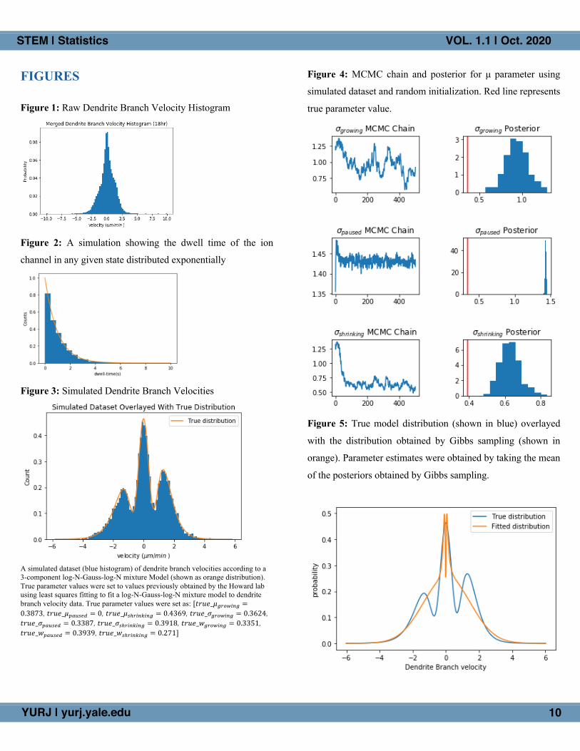
Figure 1: Raw Dendrite Branch Velocity Histogram

Figure 2: A simulation showing the dwell time of the ion

channel in any given state distributed exponentially

Figure 3: Simulated Dendrite Branch Velocities

A simulated dataset (blue histogram) of dendrite branch velocities according to a 3-component log-N-Gauss-log-N mixture Model (shown as orange distribution). True parameter values were set to values previously obtained by the Howard lab using least squares fitting to fit a log-N-Gauss-log-N mixture model to dendrite branch velocity data. True parameter values were set as: [𝑡𝑟𝑢𝑒_𝜇!"#$%&! =0.3873, 𝑡𝑟𝑢𝑒_𝜇'()*+, = 0, 𝑡𝑟𝑢𝑒_𝜇*-"%&.%&! = 0.4369, 𝑡𝑟𝑢𝑒_𝜎!"#$%&! = 0.3624, 𝑡𝑟𝑢𝑒_𝜎'()*+, = 0.3387, 𝑡𝑟𝑢𝑒_𝜎*-"%&.%&! = 0.3918, 𝑡𝑟𝑢𝑒_𝑤!"#$%&! = 0.3351, 𝑡𝑟𝑢𝑒_𝑤'()*+, = 0.3939, 𝑡𝑟𝑢𝑒_𝑤*-"%&.%&! = 0.271]

Figure 4: MCMC chain and posterior for μ parameter using

simulated dataset and random initialization. Red line represents

true parameter value.

Figure 5: True model distribution (shown in blue) overlayed

with the distribution obtained by Gibbs sampling (shown in

orange). Parameter estimates were obtained by taking the mean

of the posteriors obtained by Gibbs sampling.


Social Sciences

11


Figure 6: Simulated dataset thresholded into 3 categories

using Otsu’s method. Thresholds are k1 = -0.919 and k2 =

0.714

Figure 7: MCMC chain and posterior for 𝜇 parameter using

simulated dataset and Otsu initialization. 𝜇9:;<=> parameter

fixed to 0. Red line represents true parameter values. Green

lines represent 95% confidence intervals (values shown in

Table 1). MCMC chain run for 1000 iterations.

Figure 8: MCMC chain and posterior for σ parameter using

simulated dataset and Otsu initialization. Red line represents

true parameter values. Green lines represent 95% confidence

intervals (values shown in Table 1). MCMC chain run for 1000

iterations.


Social Sciences

12


Figure 9: MCMC chain and posterior for w parameter using

simulated dataset and Otsu initialization. Red line represents

true parameter values. Green lines represent 95% confidence

intervals (values shown in Table 1). MCMC chain run for 1000

iterations.

Figure 10: The true model distribution (shown in blue)

overlayed with the distribution obtained by Gibbs sampling

(shown in orange). Gibbs sampling with Otsu’s initialization

successfully recovers the true distribution with a KL divergence

of 0.0195.

Figure 11: MCMC chain and posterior for 𝜇 parameter using

experimentally measured dendrite branch velocity dataset and

Otsu initialization. MCMC chain was run for 1000 iterations

with effective sample sizes shown in Table 2. Red lines

represent 95% confidence intervals (values shown in Table 2).

Figure 12: MCMC chain and posterior for 𝜎 parameter using






Social Sciences

13


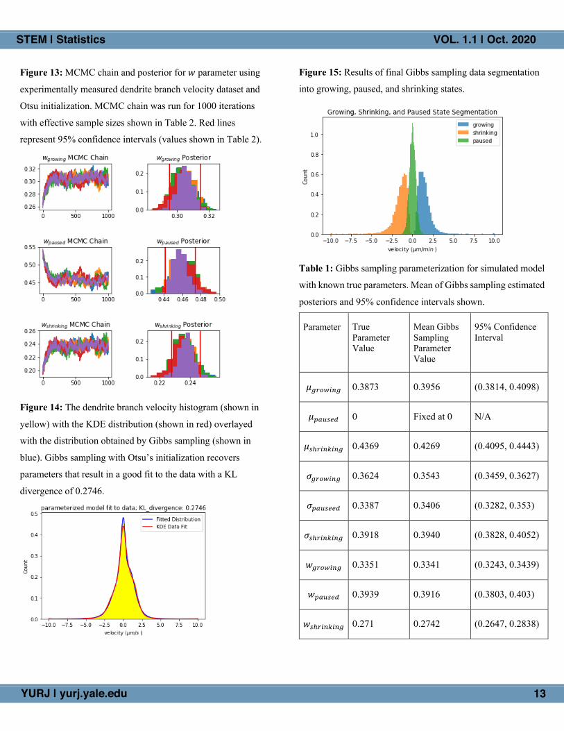
Figure 13: MCMC chain and posterior for 𝑤 parameter using





Figure 14: The dendrite branch velocity histogram (shown in

yellow) with the KDE distribution (shown in red) overlayed

with the distribution obtained by Gibbs sampling (shown in

blue). Gibbs sampling with Otsu’s initialization recovers

parameters that result in a good fit to the data with a KL

divergence of 0.2746.

Figure 15: Results of final Gibbs sampling data segmentation

into growing, paused, and shrinking states.

Table 1: Gibbs sampling parameterization for simulated model

with known true parameters. Mean of Gibbs sampling estimated

posteriors and 95% confidence intervals shown.

Parameter True Parameter Value

Mean Gibbs Sampling Parameter Value

95% Confidence Interval

𝜇4567&84 0.3873 0.3956 (0.3814, 0.4098)

𝜇9:;<=> 0 Fixed at 0 N/A

𝜇<?5&80&84 0.4369 0.4269 (0.4095, 0.4443)

𝜎4567&84 0.3624 0.3543 (0.3459, 0.3627)

𝜎9:;<==> 0.3387 0.3406 (0.3282, 0.353)

𝜎<?5&80&84 0.3918 0.3940 (0.3828, 0.4052)

𝑤4567&84 0.3351 0.3341 (0.3243, 0.3439)

𝑤9:;<=> 0.3939 0.3916 (0.3803, 0.403)

𝑤<?5&80&84 0.271 0.2742 (0.2647, 0.2838)


Social Sciences

14


Table 2: Gibbs sampling parameterization of Class IV dendrite

branch velocity data. Mean parameter values for Gibbs

sampling posterior estimates across 5 MCMC chains shown

along with 95% confidence intervals. Gelman-Rubin diagnostic

shown to assess MCMC chain convergence with a convergence

threshold of 1.1. Effective sample size shown for all parameters.

Parameter Mean Parameter Value (across 5 chains)

95% Confidence Interval (for 1 chain)

Gelman-Rubin Convergence diagnostic (r_hat < 1.1)

Effective Sample Size

(dependent sample size = 700)

𝜇4567&84 0.2609 (0.2371, 0.2794)

1.0787 63.95

𝜇9:;<=> Fixed at 0

N/A N/A N/A

𝜇<?5&80&84 0.2760 (0.2424, 0.3035)

1.0788 61.55

𝜎4567&84 0.4936 (0.4823, 0.5075)

1.0769 69.81

𝜎9:;<==> 0.3816 (0.3632, 0.3951)

1.0956 52.01

𝜎<?5&80&84 0.5514 (0.5365, 0.5689)

1.0720 68.66

𝑤4567&84 0.3039 (0.2953, 0.3148)

1.0765 67.34

𝑤9:;<=> 0.4600 (0.4414, 0.4741)

1.0921 55.67

𝑤<?5&80&84 0.2361 (0.2279, 0.2466)

1.0822 64.47

ACKNOWLEDGEMENTS I would like to thank Prof. Jonathon Howard, Olivier Trottier,

Sabya Sutradhar and the rest of the Howard lab for their support

and feedback throughout this project.

REFERENCES (1) Jan, Lily et al., 2010. Branching Out: Mechanisms of

Dendritic Arborization. Nat Rev Neurosci, Vol 11 pp. 316-328.

(2) Conde, C., Cáceres, A., 2009. Microtubule assembly,

organization and dynamics in axons and dendrites. Nat Rev

Neurosci, Vol 10 pp. 319–332.

(3) Lambert, Ben. A Students Guide to Bayesian Statistics.

SAGE, 2018.

(4) Barker, B.S. et al., 2017. Conn’s Translational

Neuroscience: Chapter 2 - Ion Channels. Academic Press. pp.

11-43.

(5) Fridman, Daniel. Bayesian Inference for the

Parameterization of Mixture Models with Biophysical

Applications, S&DS 480 Independent Study Report, Yale

University. December 2019.

(6) Hines, K., 2015. A Primer on Bayesian Inference for

Biophysical Systems. Biophysical Journal, Vol 108 pp. 2103-

2113.

(7) Jordan, M. The Conjugate Prior for the Normal

Distribution, lecture notes, Stat260: Bayesian Modeling and

Inference, UC Berkeley, delivered February 8 2010.

(8) Otsu, Nobuyuki, 1979. A Threshold Selection Method from

Gray-Level Histograms. IEEE Transactions and Systems, Vol

SMC-9 pp. 62-66.

(9) Gelman, A. Rubin, D.B., 1992. Inference from Iterative

Simulation Using Multiple Sequences. Statist. Sci., Vol 7 pp.

457-511.

(10) Kullback, S., Leibler, R.A., 1951. On Information and

Sufficieny. Annals of Mathematical Statistics. Vol 22 pp. 70-

86.


Social Sciences

15


APPENDIX

Conjugate Priors

In certain cases, an exact closed-form solution for the

posterior can be calculated without having to calculate the

marginal posterior by selecting a mathematically convenient

prior. More specifically, if a prior is chosen from a specified

family of distributions such that the posterior will fall into the

same family of distributions, it may be possible to obtain a

closed-form solution for the posterior. These ’mathematically

convenient’ priors are known as conjugate priors (2).

In order to explain how conjugate priors work, it is

easiest to use an example. Thus, I will use a biophysically

relevant example relating to ion channel patch-clamp recordings

in order to demonstrate the use of conjugate priors (5,6).

Example: Ion Channel Patch-Clamp Recording (4,5,6)

Most cells, including neurons, contain proteins called

ion channels on their membranes which allow for ions to flow

between the interior and exterior of the cell. These ion channels

regulate the concentration of ions across the membrane by

stochastically transitioning between open and closed states

according to a Poisson process. The time an ion channel spends

in any given state (dwell-time) is known to follow an

exponential distribution. An experiment can be carried out

which tracks the time spent in each state and a histogram of

dwell-times can be plotted, a simulation of which is shown in

Fig. 2.

We first model the dwell-times as random variables

from an exponential distribution, 𝑦& ∼ 𝜆𝑒%@+. For N samples,

we thus form an exponential likeihood: ∏ 𝜆#&2! 𝑒(%@+!). Next, we

seek to determine the time-scale parameter 𝜆 of our model based

on our data. We can formulate this problem in terms of Bayesian

inference as follows:

𝑝(𝜆|𝑦) ∝ (R𝜆#

&2!

𝑒(%@+!))𝑝(𝜆)

Our goal is to select an appropriate prior, 𝑝(𝜆), such

that we can obtain a closed form posterior for the time-scale

parameter, 𝑝(𝜆|𝑦). The conjugate prior to an exponential

likelihood is the Gamma distribution:

𝑝(𝜆) ∼ 𝐺𝑎𝑚𝑚𝑎(𝜆|𝛼, 𝛽) =𝛽3

𝛤(𝑎) 𝜆3%!𝑒%@A

With the following set of steps we can see how the Gamma prior conveniently combines with the exponential likelihood:

𝑝(𝜆|𝑦) ∝ (R𝜆#

&2!

𝑒(%@+!)) ×𝛽3

𝛤(𝑎) 𝜆3%!𝑒%@B

∝ (𝜆#𝑒%@∑ +!"!#$ ) × (

𝛽3

𝛤(𝑎)𝜆3%!𝑒%@B)

∝ (𝜆#𝑒%@∑ +!"!#$ )(𝜆3%!𝑒%@B)

= 𝜆3D#%!𝑒%@(∑ +!"!#$ DB)

We observe that the simplified solution above follows

the same form as the Gamma distribution, but with new

hyperparameters, updated according to our data. Thus, we

obtain the final closed-form solution for our posterior:

𝑝(𝜆|𝑦) ∼ 𝛤(𝜆|𝛼′, 𝛽′) s.t. 𝛼′ = 𝛼 + 𝑁 and 𝛽′ =[𝑦&

#

&2!

+ 𝛽

Using the idea of conjugate priors, we are able to solve

for the posterior distribution of the time-scale parameter for our

exponential model, dependent on our data of ion channel dwell-times.

Applications of Bayesian Inference for Modelling Dynamic ...

Documents

Transcript of Applications of Bayesian Inference for Modelling Dynamic ...