Application of Value Stream Mapping and Possibilities of ... · PDF fileand Possibilities of...

© Faculty of Mechanical Engineering, Belgrade. All rights reserved FME Transactions (2015) 43, 279-286 279

Received: October 2015, Accepted: November 2015 Correspondence to: Dorota Stadnicka, PhD Rzeszow University of Technology, Faculty of Mech. Eng. & Aeronautics, Al. Powstancow Warszaw 12, 35-959 Rzeszow, Poland, [email protected] doi:10.5937/fmet1504279S

Dorota Stadnicka Assistant Professor

Rzeszow University of Technology Faculty of Mechanical Engineering

and Aeronautics, Poland

Dario Antonelli

Professor Politecnico di Torino,

Department of Production Systems and Economics,

Italy

Application of Value Stream Mapping and Possibilities of Manufacturing Processes Simulations in Automotive Industry Value Stream Mapping (VSM) is a commonly assessed method employed for the analysis of manufacturing processes. The principal asset of the method is its ability to identify wastes. Adopting lean manufacturing and lean management rules it is possible to eliminate such wastes. In the paper the case study of a manufacturing process of sleeves is presented. The current value stream map (CSM) and the future value stream map (FSM) of the sleeve manufacturing process are used. They are investigated with the help of Value Stream Analysis (VSA) that assists the process designer in identification and elimination of wastes. However, the authors think that, in order to take into account all the outcomes of the VSM, the analysis should be assisted by complementary tools such as computer simulations (CSs). CSs were implemented to analyse the data concerning a manufacturing process of the sleeve in order to use the results of VSA. Keywords: Manufacturing Processes, Wastes Elimination, VSM, VSA, Discrete Events Simulation.

1. INTRODUCTION Value Stream Mapping (VSM) is a method well

assessed, together with all the tools used in value stream improvement [1, 2]. The method has been used in industry for many years [3], especially in the automotive industry [4, 5]. However, one can also find examples of VSM implementation e.g. in emergency room [6] or in the service sector [7].

The method can be implemented for manufacturing processes (MPs) [8,9,10,11], as well as for business [12] and administrative processes [13]. The implementation of the method in various groups of processes involves a few different ways of value stream implementation.

The method helps to improve manufacturing processes [14], assembly processes [15,16], processes concerning product development [17, 18] etc.

The main goal of VSM implementation is the waste identification and value stream improvement. In order to develop the value stream it is recommended to follow a set of rules [1]. These rules indicate different lean tools [19] which can be used to eliminate or at least decrease wastes in the value stream. While analysing a value stream map it is possible to identify problems to which the solution may allow the company to achieve better results. Sometimes the solution for the problems, which were discovered in the Value Stream Analysis (VSA), is apparent. Sometimes it is not so obvious which solutions are suitable in order to ensure the best performance. In such cases, it is helpful to carry out an additional analysis, namely the computer simulations

(CSs). CS saves time and gives the possibility of having a deeper insight into the process performance. Examples of the simulations implementation, together with the value stream analysis, can be found in literature [20, 21]. However, preparing a model of a manufacturing system (MS) which will be analysed in CSs is also time consuming. That is why, the question is when we really need to carry out the simulations, and when it still is not necessary.

The paper presents a case study in which the production flow of a sleeve covered by rubber (vulcanized) is analysed with the use of VSA. The discovered problems are solved with the lean tools and suggested improvements. Then, the MS is modelled with the use of FlexSimTM program used in simulations. The solutions proposed in FSM are used in CSs. The authors try to answer the questions: whether the planned results can be achieved and whether the simulation was really necessary in the case.

The authors attempt to answer the question when it is useful to adopt CSs, assess time consumption as well as the question of which cases CSs can add value to the analysis.

2. METHODS OF VSM AND VSA

VSM used in MS analyses uses standard symbols to present elements of MS as well as the standard rules of VSA, described in literature [1].

VSM is implemented for a product family, which is a group of products that go through similar MP and over common equipment in downstream processes.

In order to develop CSM it is necessary to gather information concerning the client's demands, shipment quantity and frequency, processes engaged in products manufacturing, cycle times (CTs) of processes, which give information on how often the products are

280 ▪ VOL. 43, No 4, 2015 FME Transactions

completed by processes; changeover times (COs), the number of operators, materials delivery quantity and frequency, the quantity and places of inventories, working time, problems such as quality problems, machine failures and shutdowns, etc.

In VSA it is recommended to perform such calculations as the calculation of a daily client's demand (DCD) – equation (1); available working time (AWT) – equation (2); processing time (PT) – equation (3); inventory lead times (ILTs) – equation (4); manufacturing processes lead time (LT) – equation (5); takt time (TT) – equation (6); a required number of operators (RON) – equation (7).

,WDM

CDCD N

MD = (1)

where: MCD – monthly client demand [pcs/month], NWDM – number of working days in a month [days/month].

,BWWT TTA −= (2) where: TW – working time a day [sec/day], TB – break time [sec/day].

,1∑=

=n

iiCTPT (3)

where: CT – cycle time [sec], n – a number of manufacturing processes.

,CDD

IQILT = (4)

where: IQ – inventory quantity [pcs], DCD – daily client demand [pcs/day].

,1∑=

+=n

jjILTPTLT (5)

where: PT – processing time [days], ILT – inventory lead time [days], n – number of inventory kinds.

D

WT

CATT = , (6)

where: AWT – available working time [sec/day], DCD – daily client’s demand [pcs/day].

TTPTRON = , (7)

where: RON – required number of operators, PT – processing time [sec], TT – tact time [sec].

The analysis highlights bottleneck workstations, excessive inventory levels and unnecessary frequent shipments.

Then, it should be analysed whether the MS is balanced. If possible, the flow should be implemented, in other case the Just in Time system with supermarkets and Kanban cards can be introduced to decrease the amount of inventories.

All the proposed improvements are collected and implemented in the FSM.

3. COMPUTER SIMULATIONS OF MANUFACTURING PROCESSES Computer simulation of the product flow is

a common design strategy used before launching a new production line [22]. The most frequently used simulation method is Discrete Event Simulation (DES) of the production, described as a queueing network. The main benefits of DES are the understanding of the system behavior before building it, the discovery of unexpected nonconformities, the possibility of investigating different uses of case scenarios [23]. The main drawback is obviously related to the extent to which the simulation can be made compatible with the current system.

This drawback is particularly significant when DES is applied to a process model described by VSM. The goals of the two methods are different, and that is reflected in the kind of data collected by VSM which are different from the data needed by DES. VSM aims at identifying the unnecessary processes (with no added value) and tasks with average cycle times, while DES focuses on the queueing network and, therefore, requires cycle times distribution and interarrival times distribution. Nevertheless, there are several examples of simulations applied to VSM, especially in order to verify the outcomes of FSM [20, 24]. Obviously, it is necessary to acquire additional datasets with respect to the data provided by VSM.

The goal of the study was to analyse the CSM of the sleeves manufacturing process, to identify the existing wastes, to analyse the problems as well as the present suggestions for a value stream development on FSM.

In the research it was decided to apply VSM, VSA and CSs in order to see the added value of each tool. CSM and FSM are generated with Microsoft Visio Professional, while FlexSimTM is employed for CSs.

4. SLEEVES’ MANUFACTURING

Rubber-metal sleeves (Figure 1) are an assembly element for a car frame (commonly named silent-blocks). The product is delivered to customer in two shapes. Orders are stable. A monthly customer's order amounts to 16,000 pcs equally divided between two types.

The orders are loaded on the supplier’s MRP system (SAP). The production orders are generated monthly, and the weekly orders or shift orders go to each work stand.

Products are delivered in containers of 2,000 pcs. The containers are returnable. Sleeves are shipped once a week. The customer sends a monthly forecast and a weekly order.

Materials needed for manufacturing are delivered from an internal supplier i.e. another department in the factory. The supplier delivers internal and intermediate sleeves a few times a week.

The daily customer's demand (DCD) can be calculated from equation (1) and it equals 800 pcs/day.

The company works 20 days per month, 5 days per week, 3 shifts per day and 8 hours per shift.

FME Transactions VOL. 43, No 4, 2015 ▪ 281

Figure 1. Section of a rubber-metal sleeve, type ZE1

Manufacturing of the sleeve consists of the

processes presented in Table 1. Table 1. Manufacturing processes realized in sleeves production

Process Goal of the process Degreasing Degreasing of metal parts which can be made

on a vibratory feeder. The process consists of the following operations: removing impurities, washing, drying.

Sand-blasting The process aims at the surface cleaning with the use of abrasive material or at the surface forming by abrasive actions or grinding.

Phosphatizing Chemical treatment to protect the product surface from corrosion. After the process the surface is prepared for adhesive coating.

Adhesive coating

Adhesive is warmed. The filings are eliminated in the machine.

Vulcanization In the process metal elements are glued with rubber elements. 36 pieces can be in the process at the same time. The last operation of the process is products marking. Each product is marked with a blue dot.

Adhesion testing

Rubber adhesion is tested.

Control and Packing

The products are 100% visually controlled. Next, the products are packed to special containers according to the customer's requirements.

Shipment Shipment to a customer is realized once a week. For shipments FIFO is applied.

The product consists of two metal elements (internal

sleeve and intermediate sleeve). They are treated in different processes. Data concerning the processes are presented in Table 2, Table 3 and Table 4. The number of operators on the production line is 12. The workflow is presented in Figure 2.

The inventory in time units (ILT) have been calculated from equation (4).

The full CSM visible in the whole MS and in the warehouse, as well as ILTs are presented in Figure 3.

Table 2. Manufacturing processes of internal and intermediate sleeves and additional data concerning the processes

Symbol Process Additional data

DIS Degreasing of internal sleeve

Automatic process

SIS Sand-blasting of internal sleeve

Automatic process

PIS Phosphatizing of internal sleeve

Automatic process

AIS Adhesive coating of internal sleeve

Automatic process.

DES Degreasing of intermediate sleeve

Automatic process

SES Sand-blasting of intermediate sleeve

Automatic process

PES Phosphatizing of intermediate sleeve

Automatic process

AES Adhesive coating of intermediate sleeve

Automatic process

BM Building of the mixture Manual process VLC Vulcanization Partly automatic and

partly manual process AT Adhesion testing Mechanized process SP Shipment Inventory of products

ready for shipment Table 3. Times concerning manufacturing processes and number of operators

Symbol

Cycle time for

one piece CT

[sec]

Cycle time for a batch CTs [sec]

Lead time of

the process

[sec]

Setup time CO [h]

Number of

operatorNo

DIS 6 2 544 2 544 0 1 SIS 5.4 2 290 2 290 0 1 PIS 11.4 4 766 4 766 0 1 AIS 8.11 3 408 48.7 1.5-2 2 DES 5 2 124 2 124 0 1 SES 9.8 4 090 4 090 0 1 PES 11.4 4 766 4 766 0 1 AES 4.91 2 062 343.7 1.5-2 1 VLC 34.6 1 248 1 248 8 2 AT 12.2 439.2 439.2 0.25 1

Accessibility of all work stands is 100%,

Table 4. Size of batches in sleeves manufacturing line

Symbol

Size of a transportation

batch to the process

[pcs]

Size of a transportation batch after the

process [pcs]

Number of pieces in

the process at the same

time DIS 420 420 420 SIS 420 420 420 PIS 420 420 420 AIS 420 36 6 DES 420 420 420 SES 420 420 420 PES 420 420 420 AES 420 70 70 VLC 36 36 36 AT 36 36 1


DIS SIS PIS AIS

VLC AT

DES SES PES AES

ShipmentSP

Figure 2. Workflow

We can see huge inventories before degreasing processes (DIS, DES), vulcanization (VLC) and adhesive testing (AT). It means that these processes are usually slower than the upstream processes. 5. ANALYSIS OF CURRENT STATE AND

PROBLEMS IDENTIFICATION

In order to identify problems in the current state of a value stream, first of all, it is necessary to calculate TT from the equation (6). The calculations are presented in equation (8).

pcsTT sec/98pcs/day800

sec/shift 10026shifts/day 3=

⋅= (8)

We already know that TT equals 98 sec. We can compare CTs of MPs in order to assess if a bottleneck process exists in the production line. The analysis of cycle times for the analysed case is presented in Figure 4.

On the basis of the performed time analysis it can be said that there are no undersized processes and the company shouldn’t have any problems with deliveries to a customer, because the TT (TT = 98 sec) is much higher than CTs of the processes. Furthermore, the utilization rate (UR) of the processes is very low. In this situation the company could probably increase the production rate safely.

Figure 4. Analysis of cycle times

From VSM it is apparent that the manufacturing line is not balanced. VLC process takes much more time than other processes. This is the slowest process in the MS and it decreases a throughput rate (TR).

The required number of operators for the line (RON) can be calculated from equation (7) in 1.32, i.e. 2 operators.

In the current situation it would be enough to engage 2 operators to perform the work on the production line. We observe different kinds of wastes such as operators waiting for work, processes stoppage while waiting for semi-products, materials waiting to be processed and products waiting to be shipped to a customer. We also see long COs in the adhesive coating processes (AIS, AES) and in VLC.

In order to decrease inventories and to improve the flow in MS a FSM was proposed. It is presented in Figure 5. It was decided to produce DIS and DES on one work stand only as both have a low utilization level. It is possible because a changeover is not needed while the production changes from DIS to DES.

Suppliers

Production control

45.2 days 0.9 days 06 sec

(2 544 sec)5.4 sec

(2 290 sec)11.4 sec

(4 766 sec)

116.6 days

108.82 sec

DIS

Weekly order

Shipment

19.7 days

36 120 pcs

VLC

DES SES PES AES

AT

28 100 pcs

SIS PIS

Daily shipping schedule

CT = 6 sec

CsT = 2 544 sec

CO = 0

5 days, 3 shifts

AWT = 26 100 sec

CT = 5 sec

CsT = 2 124 sec

CO = 0

5 days, 3 shifts

AWT = 26 100 sec

CT = 5.4 sec

CsT = 2 290 sec

CO = 0

5 days, 3 shifts

AWT = 26 100 sec

CT = 9.8 sec

CsT = 4 090 sec

CO = 0

5 days, 3 shifts

AWT = 26 100 sec

CT = 11.4 sec

CsT = 4 766 sec

CO = 0

5 days, 3 shifts

AWT = 26 100 sec

CT = 8.11 sec

CsT = 3 408 sec

CO = 1.5 – 2 hours

5 days, 3 shifts

AWT = 26 100 sec CT = 34.6 sec

CTs = 1 248 sec

CO = 8 hours

5 days, 3 shifts

AWT = 26 100 sec

CT = 12.2 sec

CTs = 439.2 sec

CO = 0.25 hours

5 days, 3 shifts

AWT = 26 100 sec

Weekly schedule

Daily order

Monthly forecast

Monthly forecast

CT = 11.4 sec

CsT = 4 766 sec

CO = 0

5 days, 3 shifts

AWT = 26 100 sec

CT = 4.91 sec

CsT = 2 062 sec

CO = 1.5 – 2 hours

5 days, 3 shifts

AWT = 26 100 sec

3.4 days8.11 sec

(3 408 sec)

44.9 days

35.2 days 0.2 days 05 sec

(2 124 sec)9.8 sec

(4 090 sec)11.4 sec

(4 766 sec)

2.7 days4.91 sec

(2 062 sec)

8 days34.6 sec

(1 248 sec)

2.3 days

12.2 sec(439.2 sec)

AIS

2

2

656 pcs 0 pcs 2 704 pcs

35 900 pcs

140 pcs 0 pcs 2 180 pcs

6 362 pcs

18 754 pcs 15 763 pcs

Customer

16 000 pcs/month

4 000 pcs/week

800 pcs/day

One container = 2 000 pcs

Figure 3. Current state map


Suppliers Customer

Production control

0.525 days 0.525 days6 sec

(2 544 sec)5.4 sec

(2 290 sec)11.4 sec

(4 766 sec)

5.225 days

108.82 sec

Weekly order

Shipment

1.25 days

VLCDS SS PS AES AT

Daily shipping schedule

CT = 5 sec

CsT = 2 124 sec

CO = 0

5 days, 3 shifts

AWT = 26 100 sec

CT = 9.8 sec

CsT = 4 090 sec

CO = 0

5 days, 3 shifts

AWT = 26 100 sec

CT = 8.11 sec

CsT = 3 408 sec

CO = 1.5 – 2 hours

5 days, 3 shifts

AWT = 26 100 sec

CT = 34.6 sec

CTs = 1 248 sec

CO = 8 hours

5 days, 3 shifts

AWT = 26 100 sec

CT = 12.2 sec

CTs = 439.2 sec

CO = 0.25 hours

5 days, 3 shifts

AWT = 26 100 sec

Weekly schedule

Daily order

Monthly forecast

Monthly forecast

CT = 11.4 sec

CsT = 4 766 sec

CO = 0

5 days, 3 shifts

AWT = 26 100 sec

CT = 4.91 sec

CsT = 2 062 sec

CO = 1.5 – 2 hours

5 days, 3 shifts

AWT = 26 100 sec

0.525 days8.11 sec

(3 408 sec)

0.625 day

4.91 sec(2 062 sec)

34.6 sec(1 248 sec)

1.25 days12.2 sec

(439.2 sec)

16 000 pcs/month

4 000 pcs/week

800 pcs/day

One container = 2 000 pcs

AIS

420 pcs

500 pcs

420 pcs

FIFO

max 1000 pcs

FIFO

max 1000 pcsFIFO

max 420 pcs

FIFO

max 420 pcs

500 pcs

0.525 days

0.525 days

2

2

0.625 day

Figure 5. Future state map

Additionally, CTs are the same for both, internal and

intermediate sleeves. The similar situation occurs between SIS and SES as well as between PIS and PES. However, CT of SES is almost as twice long as CT of SIS. AIS and AES have to be realized on different machines because the processes for internal sleeves and intermediate sleeves are different, and adhesive coating process of both can’t be realized on the same machine – not on any of the existing machines. In the FSM it is also proposed to implement supermarkets with Kanban cards and FIFO lanes in order to decrease inventories. After the implementation of the solutions presented in FSM, it will be possible to decrease LT of the production process. In CSM LT equals 116.6 days, while in FSM it is only 13.31 days. 6. GENERAL DISCUSSION

VSA aims at identifying three types of activities in the production flow: 1-non value added; 2-necessary but non value added; 3-value added. There are seven sources of waste: overproduction, waiting, transport, inappropriate processing, unnecessary inventory, unnecessary motion, defects [19].

The rationale is to eliminate 1 and to shorten the time spent by 2, or even reorganize the flow in order to avoid the necessity of type 2 activities. The activities are tagged by their LT. The LT could be the time allotted for the processing by managers or the actual average time measured in practice.

As VSM was originally applied to the factories that followed the Toyota Production System paradigm, the choice of not considering the process variability but only the mean time was not seen as a vice. Toyota Production System aims at eliminating every source of variability as the main cause of Muda.

Nevertheless, the large success of VSM extended its application to many small and medium enterprises as well as to several production and services sectors, where Toyota Production System cannot be applied directly. This is the case of the present enterprise.

In order to correctly estimate the amount of non-value added time, in the presence of variable process times, it is necessary to calculate the average waiting time on a line. The queueing theory, for a Markovian process with Markovian arrivals, and a First in First out (FIFO) queue policy says that the average time in a queue tqueue is calculated from equation (9).

equeue tUR

URMMt ⋅−

=1

)1//( (9)

where: te is the effective mean process time.

It is clear that the time wasted in a queue is not a function of the mean process time only, but it strongly depends on UR. When UR approaches the unity, the time in a queue tends toward infinity.

Therefore, in a real factory producing small batches with a changing demand volume, the queue time is not constant but it increases nonlinearly with the demand growth. This effect could be overlooked by VSM. The increase in the demand is observed only in terms of the reduced takt time (TT). Because of queue explosion it is possible that the production cannot meet the demand even if CT is well below TT.

Let us assume that we are not able to eliminate all the queues before the processes. If this is the case, VSM would yield misleading recommendations unless not supported by a classic process simulation by the means of a queueing theory.


7. COMPUTER SIMULATIONS OF PRODUCTION LINE WORKING

In the present case study the process is simulated with exponential process time distribution, neglecting the time increase due to preemptive outages.

On the basis of the data gathered from MS and presented in previous tables, the model of MS was developed.

Then the simulation of work for the current state (CS) and future state (FS) was performed. The simulation covers one week. The experiment was conducted by assuming different scenarios with the increasing arrival rate of raw materials. In the first scenario, S1, the arrival rate is equal to the observed rate, in the fourth scenario, S4, the rate is quadrupled, as shown in Figure 6.

Figure 6. Cumulative production orders vs. time for four different scenarios

The model of a production line is presented in Figure 7 and the simulations results are presented in Tables 5-11.

It is possible to show how the arrival rate influences Work In Progress (WIP), throughput rate (TR) and utilization rate (UR) of the vulcanization workstation in the different scenarios.

The forth scenario deliberately stresses the production line above its capacity. In S4, VLC has an UR equal to 1 and, therefore, WIP explodes, while TR is bounded to the bottleneck rate, i.e. VLC’s capacity.

Table 5. WIP [pcs] – CS

Mean (90% Confidence) Sample Std Dev Min Max

S1 2327 < 2330 < 2332 8.1 2316 2350

S2 2609 < 2612 < 2614 8.9 2599 2633

S3 4352 < 4360 < 4369 28 4320 4424

S4 16969 < 16977 < 16985 25 16941 17033

Table 6. WIP [pcs] – FS


S1 2906 < 2908 < 2910 6.5 2901 2934

S2 2714 < 2716 < 2719 8.7 2701 2742

S3 4708 < 4717 < 4726 28 4685 4814

S4 17121 < 17132 < 17142 34 17080 17230

From Tables 5 and Tables 6 we can draw

conclusions that WIP in CS and FS are similar in each simulation (Figure 8). This is counterintuitivebecause in FS most inventories are strictly bounded to contain 1 batch.

Figure 8. Graphical comparison of WIP in the 4 scenarios between CS and FS

The reason is that the inventories in the internal and intermediate sleeve production line are hardly ever used as the UR of the corresponding workstations is very low and, therefore, only the inventories supplyingthe VLC are actually used.

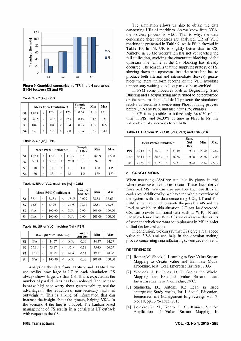
TR is the same in all simulations in both cases (CS and FS) (Figure 9), and in the last two scenarios it is saturated to the bottleneck rate that is 105 items/hour.

Figure 7. A model of production line in FlexSim

CP AT

VLC

AIS PIS SIS DIS

AESPES SES

DES


Figure 9. Graphical comparison of TR in the 4 scenarios S1-S4 between CS and FS

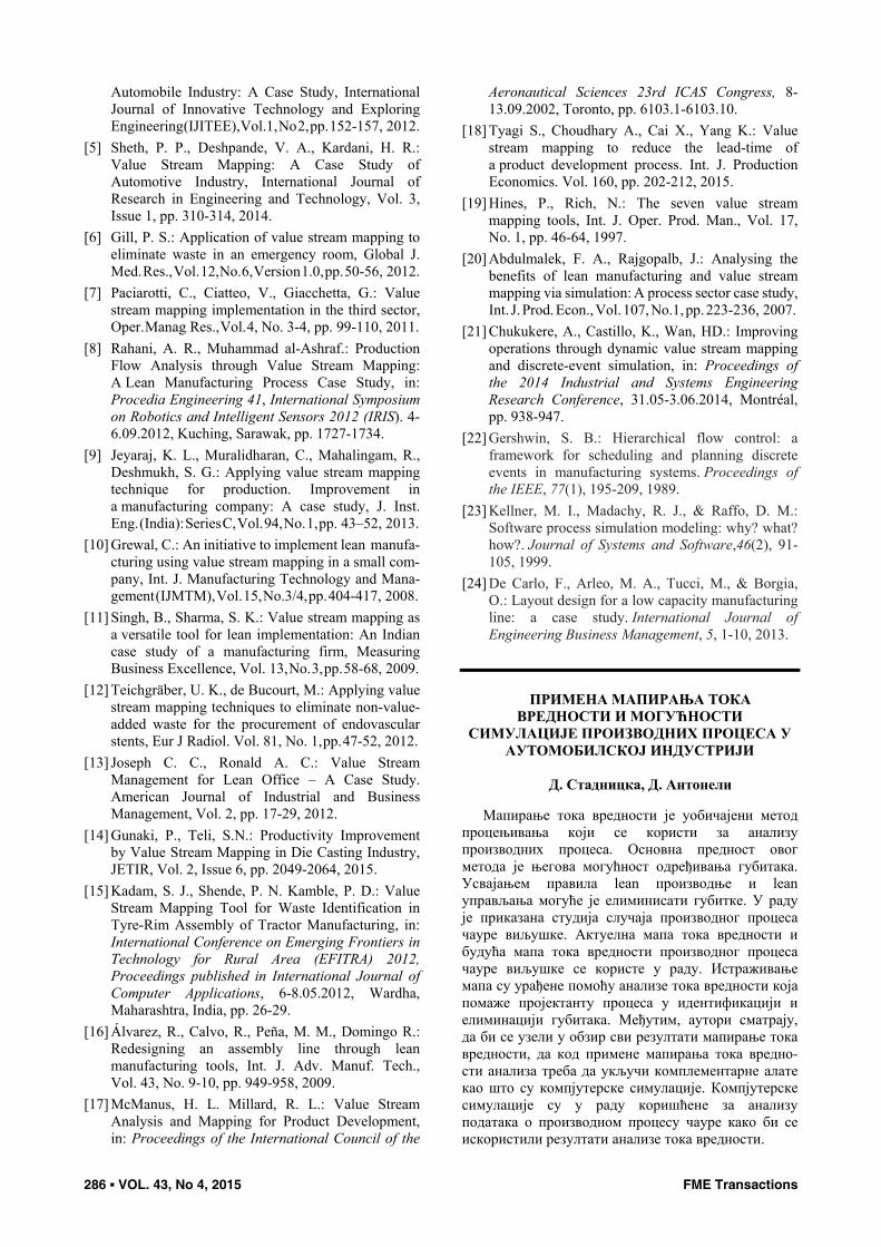
Table 7. LT [ks] – CS


S1 119.8 < 120 < 120 0.60 18.8 121

S2 92.2 < 92.3 < 92.4 0.43 91.5 93.3

S3 104 < 104 < 104 0.95 103 106

S4 337 < 338 < 338 1.06 333 340

Table 8. LT [ks] – FS


S1 169.8 < 170.1 < 170.3 0.8 168.9 172.8

S2 97.8 < 97.9 < 98.0 0.3 97 99

S3 110 < 111 < 111 1.0 110 115

S4 180 < 181 < 181 1.0 179 183

Table 9. UR of VLC machine [%] – CSM


S1 38.4 < 38.52 < 38.55 0.099 38.33 38.62

S2 55.8 < 55.96 < 56.04 0.257 55.31 56.58

S3 N/A < 100.00 < N/A 0.00 100.00 100.00

S4 N/A < 100.00 < N/A 0.00 100.00 100.00

Table 10. UR of VLC machine [%] – FSM


S1 N/A < 34.57 < N/A 0.00 34.57 34.57

S2 55.81 < 55.87 < 55.9 0.21 55.43 56.35

S3 98.9 < 98.93 < 99.0 0.25 98.11 99.40

S4 N/A < 100.00 < N/A 0.00 100.00 100.00

Analysing the data from Table 7 and Table 8 we can realize how large is LT in each simulation. FS always shows larger LT than CS. This is expected as the number of parallel lines has been reduced. The increase is not as high as to worry about system stability, and the advantages in the reduction of non-necessary machines outweigh it. This is a kind of information that can increase the insight about the system, helping VSA. In the scenario 4 the line is blocked. The kanban based management of FS results in a consistent LT cutback with respect to the CS.

The simulation allows us also to obtain the data concerning URs of machines. As we know from VSA, the slowest process is VLC. That is why, the data concerning these processes are analysed. UR of VLC machine is presented in Table 9, while FS is showed in Table 10. In FS, UR is slightly better than in CS. Namely, in S3 the workstation has not yet reached the full utilization, avoiding the concurrent blocking of the upstream line; while in the CS blocking has already occurred. The reason is that the supplyingstrategy of FS, slowing down the upstream line (the same line has to produce both internal and intermediate sleeves), guara-ntees the more uniform feeding of the VLC avoiding unnecessary waiting to collect parts to be assembled.

In FSM some processes such as Degreasing, Sand Blasting and Phosphatizing are planned to be performed on the same machine. Table 11 presents the simulation results of scenario 3 concerning Phosphatizing process before (PIS and PES) and also after (PS) changes.

In CS it is possible to utilize only 36.61% of the time in PIS, and 36.33% of time in PES. In FS this value obviously increases to 71.84%.

Table 11. UR from S1 – CSM (PIS, PES) and FSM (PS)

Mean (90% Confidence) Sam. Std Dev

Min Max

PIS 36.13 < 36.61 < 37.10 0.84 35.50 37.89

PES 36.11 < 36.33 < 36.56 0.38 35.76 37.03

PS 71.30 < 71.84 < 72.37 0.92 70.22 73.12

8. CONCLUSIONS

When analysing CSM we can identify places in MS where excessive inventories occur. These facts derive from real MS. We can also see how high are ILTs in each area. Additionally, we have the whole overview of the system with the data concerning COs, LT and PT. FSM is the map which presents the possible MS and the level to which, in this situation, LT can be decreased. CSs can provide additional data such as WIP, TR and UR of each machine. With CSs we can assess the results of changes which we want to implement in MS in order to find the best solution.

In conclusion, we can say that CSs give a real added value to VSA and can help in the decision making process concerning a manufacturing system development.

REFERENCES

[1] Rother, M., Shook, J.: Learning to See: Value Stream Mapping to Create Value and Eliminate Muda. Brookline, MA: Lean Enterprise Institute, 2003.

[2] Womack, J. P., Jones, D. T.: Seeing the Whole: Mapping the Extended Value Stream. Lean Enterprise Institute, Cambridge, 2002.

[3] Stadnicka, D., Antosz, K.: Lean in large enterprises: Study results, Int. J. Social, Education, Economics and Management Engineering, Vol. 7, No. 10, pp.1376-1382, 2013.

[4] Belokar, R. M., Kharb, S. S., Kumar, V.: An Application of Value Stream Mapping In


Automobile Industry: A Case Study, International Journal of Innovative Technology and Exploring Engineering (IJITEE), Vol.1, No 2, pp. 152-157, 2012.

[5] Sheth, P. P., Deshpande, V. A., Kardani, H. R.: Value Stream Mapping: A Case Study of Automotive Industry, International Journal of Research in Engineering and Technology, Vol. 3, Issue 1, pp. 310-314, 2014.

[6] Gill, P. S.: Application of value stream mapping to eliminate waste in an emergency room, Global J. Med. Res., Vol. 12, No. 6, Version 1.0, pp. 50-56, 2012.

[7] Paciarotti, C., Ciatteo, V., Giacchetta, G.: Value stream mapping implementation in the third sector, Oper. Manag. Res., Vol. 4, No. 3-4, pp. 99-110, 2011.

[8] Rahani, A. R., Muhammad al-Ashraf.: Production Flow Analysis through Value Stream Mapping: A Lean Manufacturing Process Case Study, in: Procedia Engineering 41, International Symposium on Robotics and Intelligent Sensors 2012 (IRIS). 4-6.09.2012, Kuching, Sarawak, pp. 1727-1734.

[9] Jeyaraj, K. L., Muralidharan, C., Mahalingam, R., Deshmukh, S. G.: Applying value stream mapping technique for production. Improvement in a manufacturing company: A case study, J. Inst. Eng. (India): Series C, Vol. 94, No. 1, pp. 43–52, 2013.

[10] Grewal, C.: An initiative to implement lean manufa-cturing using value stream mapping in a small com-pany, Int. J. Manufacturing Technology and Mana-gement (IJMTM), Vol. 15, No.3/4, pp. 404-417, 2008.

[11] Singh, B., Sharma, S. K.: Value stream mapping as a versatile tool for lean implementation: An Indian case study of a manufacturing firm, Measuring Business Excellence, Vol. 13, No. 3, pp. 58-68, 2009.

[12] Teichgräber, U. K., de Bucourt, M.: Applying value stream mapping techniques to eliminate non-value-added waste for the procurement of endovascular stents, Eur J Radiol. Vol. 81, No. 1, pp. 47-52, 2012.

[13] Joseph C. C., Ronald A. C.: Value Stream Management for Lean Office – A Case Study. American Journal of Industrial and Business Management, Vol. 2, pp. 17-29, 2012.

[14] Gunaki, P., Teli, S.N.: Productivity Improvement by Value Stream Mapping in Die Casting Industry, JETIR, Vol. 2, Issue 6, pp. 2049-2064, 2015.

[15] Kadam, S. J., Shende, P. N. Kamble, P. D.: Value Stream Mapping Tool for Waste Identification in Tyre-Rim Assembly of Tractor Manufacturing, in: International Conference on Emerging Frontiers in Technology for Rural Area (EFITRA) 2012, Proceedings published in International Journal of Computer Applications, 6-8.05.2012, Wardha, Maharashtra, India, pp. 26-29.

[16] Álvarez, R., Calvo, R., Peña, M. M., Domingo R.: Redesigning an assembly line through lean manufacturing tools, Int. J. Adv. Manuf. Tech., Vol. 43, No. 9-10, pp. 949-958, 2009.

[17] McManus, H. L. Millard, R. L.: Value Stream Analysis and Mapping for Product Development, in: Proceedings of the International Council of the

Aeronautical Sciences 23rd ICAS Congress, 8-13.09.2002, Toronto, pp. 6103.1-6103.10.

[18] Tyagi S., Choudhary A., Cai X., Yang K.: Value stream mapping to reduce the lead-time of a product development process. Int. J. Production Economics. Vol. 160, pp. 202-212, 2015.

[19] Hines, P., Rich, N.: The seven value stream mapping tools, Int. J. Oper. Prod. Man., Vol. 17, No. 1, pp. 46-64, 1997.

[20] Abdulmalek, F. A., Rajgopalb, J.: Analysing the benefits of lean manufacturing and value stream mapping via simulation: A process sector case study, Int. J. Prod. Econ., Vol. 107, No.1, pp. 223-236, 2007.

[21] Chukukere, A., Castillo, K., Wan, HD.: Improving operations through dynamic value stream mapping and discrete-event simulation, in: Proceedings of the 2014 Industrial and Systems Engineering Research Conference, 31.05-3.06.2014, Montréal, pp. 938-947.

[22] Gershwin, S. B.: Hierarchical flow control: a framework for scheduling and planning discrete events in manufacturing systems. Proceedings of the IEEE, 77(1), 195-209, 1989.

[23] Kellner, M. I., Madachy, R. J., & Raffo, D. M.: Software process simulation modeling: why? what? how?. Journal of Systems and Software,46(2), 91-105, 1999.

[24] De Carlo, F., Arleo, M. A., Tucci, M., & Borgia, O.: Layout design for a low capacity manufacturing line: a case study. International Journal of Engineering Business Management, 5, 1-10, 2013.

ПРИМЕНА МАПИРАЊА ТОКА

ВРЕДНОСТИ И МОГУЋНОСТИ СИМУЛАЦИЈЕ ПРОИЗВОДНИХ ПРОЦЕСА У

АУТОМОБИЛСКОЈ ИНДУСТРИЈИ

Д. Стадницка, Д. Антонели

Мапирање тока вредности је уобичајени метод процењивања који се користи за анализу производних процеса. Основна предност овог метода је његова могућност одређивања губитака. Усвајањем правила lean производње и lean управљања могуће је елиминисати губитке. У раду је приказана студија случаја производног процеса чауре виљушке. Актуелна мапа тока вредности и будућа мапа тока вредности производног процеса чауре виљушке се користе у раду. Истраживање мапа су урађене помоћу анализе тока вредности која помаже пројектанту процеса у идентификацији и елиминацији губитака. Међутим, аутори сматрају, да би се узели у обзир сви резултати мапирање тока вредности, да код примене мапирања тока вредно-сти анализа треба да укључи комплементарне алате као што су компјутерске симулације. Компјутерске симулације су у раду коришћене за анализу података о производном процесу чауре како би се искористили резултати анализе тока вредности.

Application of Value Stream Mapping and Possibilities of ... · PDF fileand Possibilities of...

Documents

Transcript of Application of Value Stream Mapping and Possibilities of ... · PDF fileand Possibilities of...