1 INTRODUCTION

The concept of bounding surface plasticity was first introduced by Dafalias & Popov (1975) and Krieg (1975) to model nonlinear behavior of metals. In this framework, the plastic deformation at any stress point is calculated by defining the plastic modulus as a decreasing function of the distance of the stress point from its “image point” on a limiting surface called the bounding sur-face. This provides a smooth transition of stiffness from elastic to elastic-plastic state. By using a three-segmented bounding surface with a simple radial projection rule and a distance depend-ent additive plastic modulus, Dafalias & Hermann (1980) applied the theory of bounding surface plasticity to cohesive soils. Later, Bardet (1986) extended the application of the bounding sur-face models to nonlinear irreversible behavior of sands, including strain softening and stress dilatancy as observed in loose and dense sands, respectively. This was achieved by defining the plastic modulus as a function of the mean effective stress and the stress ratio. However, the model proposed was based on the associativity of flow rule, and therefore was unable to capture the post-peak strain-softening behavior of loose sands under undrained shearing. Further devel-opments on the bounding surface model were made by Crouch (1994) for 2D cases and Crouch & Wolf (1994a&b) for 3D cases, in which the combined radial and deviatoric mapping rules, non-associate flow rule, the bi-linear critical state line and the apparent normal consolidation line for sands were included. The shortcomings of this model were the complex shape of bound-ing surface, lack of continuity between the two mapping regions used in the model and the large number of model parameters.

More recently, a more rigorous bounding surface model based on the concept of the critical state soil mechanics has been developed at the University of New South Wales (UNSW) by Russell & Khalili (2004) to model the stress-strain behavior of sands. Later Khalili et al. (2005 & 2008) extended the model to simulate the behavior of sands subjected to cyclic loading under saturated and unsaturated states including hydraulic hysteresis effects. In this model, hereafter referred to as UNSW constitutive model, the shape of the bounding surface was obtained from experimental observations of undrained stress path responses of soils at their loosest state. A mapping rule, passing through stress reversal points, was introduced to predict the stress-strain

Application of the UNSW bounding surface plasticity model for clays and sands under complex stress paths

M.E. Kan & H.A. Taiebat The University of New South Wales, Sydney, NSW, Australia

ABSTRACT: This paper presents a bounding surface plasticity model that can be used to simu-late complex monotonic and cyclic loading paths. This model is formulated in the critical state framework and properly implemented using finite difference integration scheme in FLAC. The performance of the model is demonstrated using the results of experimental tests with various stress paths conducted under both monotonic and cyclic loading conditions on both sands and clays. The paper demonstrates the efficiency of the model and the implementation scheme in capturing the characteristic features of the behavior of a variety of soil types under various load-ing conditions. This model is suitable for simulation of highly erratic cyclic loading condition, e.g. those induced by earthquake or traffic loading.

behavior under loading and unloading conditions. Compared to the classical bounding surface models, UNSW model can very well capture the characteristic features of granular soils subject-ed to cyclic loading, e.g. the contraction during deviatoric unloading, as well as the behavior of normally and over consolidated clayey materials. However, the mapping rule adopted in the original UNSW model, despite its excellent performance, is not efficient for simulation of boundary value problems with highly variable loading paths due to its complex procedure and the storage and memory requirement. To tackle this problem, a new mapping rule with a single stress point was introduced by Kan et al. (2013) with a simpler procedure which is more effi-cient in problems with complex loading paths. This version of the model is implemented in FLAC (Itasca 2008) using the forward Euler finite difference integration scheme.

In the present paper, a general description of the model framework is presented first, and then a host of simulations, for a variety of different stress paths on clays and sands are presented to highlight the capabilities of the model. A single set of parameters are used for each material in all simulations, though the experimental data are taken from different sources in the literature.

2 MODEL DESCRIPTION

2.1 Notation

Soil mechanics sign is adopted throughout this paper; compression is taken as positive and ten-sion as negative. For the sake of simplicity, all derivations are presented in the q – p' plane in a three-dimensional stress space such that

2, 33

Ip q J

(1)

where I' is the first invariant of the effective stress tensor and J2 is the second invariant of the deviator stress tensor. The corresponding strain conjugates are

2

2,

3v qI J (2)

where I and J2 are the first and the second invariants of the strain vector, respectively. The in-crement of total strain is divided into elastic and plastic components as

e p (3)

where the superscripts e and p denote the elastic and plastic components, respectively. The vol-umetric strain is related to the specific volume as

0

ln( )v

(4)

where = 1e is the specific volume and e is the void ratio. o denotes to the specific volume at p = 1 kPa. The material behavior is assumed isotropic and rate independent.

2.2 Critical state and limiting isotropic compression line

Figure 1(a) shows the Critical State Line (CSL) in the ln p plane, approximated by two line-ar segments. The dimensionless state parameter ( ) of Been & Jefferies (1985) is used as a measure of consistency of the soil under its current state. The CSL in the q p plane is defined as a straight line passing through the origin, Figure 1(b), and the slope of the CSL is defined as a function of Lode angle,

1

44

max 4 4

2

1 1 sin3csM M

(5)

where is the Lode angle, ranging from 6 for triaxial extension to 6 for triaxial com-pression. is a function of the strength parameter of soil and can be given as

3 sin

3 sin

cs

cs

(6)

where cs is the critical state internal frictional angle and is considered independent of crushing of particles.

The Limiting Isotropic Compression Line (LICL) is defined as parallel to the CSL with a constant shift along the recompression line, as shown in Figure 1(a). The LICL is a reference line which can be viewed as locus of the loosest possible state for a soil under a given mean ef-fective stress.

plnkPap 1

cr

0

CSL

cr

LICL00

pcr

pc

pc

R

p

q

pc

)(csM

)(csMn

'

'

New Center ofHomology

n

LoadingSurface

New LoadingSurface

BoundingSurface

'1

'1

2

2

n1

n1

2

2

First Center ofHomology

(a)

(b)

Figure 1. (a) Critical State Line (CSL) and Limiting Isotropic Compression Line (LICL); (b) Loading surface and mapping rule for first time loading (point 1) and unloading/reloading (point 2).

2.3 Elasto-plastic behavior

The essential elements of a bounding surface plasticity model are: (i) a bounding surface for de-scribing the limit states of stress; (ii) a loading surface on which the current stress state lies and a mapping rule to find the image point on the bounding surface; (iii) a plastic potential for de-scribing the mode and magnitudes of plastic deformations, and (iv) a hardening rule for control-ling the size of the bounding surface.

In UNSW model, pure elastic response does not exist and all deformations are considered to be elastic-plastic. This is achieved by defining the hardening modulus, h, as a decreasing func-tion of the distance between the stress state and an “image point” on the bounding surface. Dur-ing loading the size of the loading surface increases so that any unloading/reloading results in elastic-plastic deformation. Definitions of the bounding surface, the loading surface and map-ping rule, the plastic potential, and the hardening rule are given in the following sections. The stress conditions on the bounding surface are denoted using a superimposed bar throughout this notes.

2.3.1 Bounding surface The shape of the bounding surface can be determined from the undrained response of the mate-rial at its loosest stat, since the undrained response of the material in the effective stress space follows the bounding surface when the contribution of elasticity to volume change is negligible. Examining a host of experimental data, Russell & Khalili (2004) and Khalili et al. (2005) sug-gested the following expression for the shape of the bounding surface:

ln, , , 0

ln

N

c

c

cs

p pqF p q p

RM p

(7)

The parameter cp controls the size of the bounding surface and is a function of the plastic volumetric strain. The material constant R is a parameter used to define the position of LICL in

ln p plane, and the constant N controls the curvature of the bounding surface.

2.3.2 Loading surface and mapping rule The loading surface is assumed to be of the same shape as the bounding surface. For first time loading these two surfaces are homologous about the origin of stress coordinate system. In this case, the function for the loading surface takes the form of

ln, , , 0

ln

N

c

c

cs

p pqf p q p

M p R

(8)

where cp is the isotropic hardening parameter controlling the size of the loading surface as il-lustrated in Figure 1(b). The state of stress is always located on the loading surface. An image for the state of stress can be found on the bounding surface as shown in Figure 1(b). The centre of homology is used to define the mapping rule. For unloading and reloading conditions, the centre of homology moves to the last point of stress reversal. The point of stress reversal is iden-tified when the product of the normal vector to the bounding surface

and the vector of the stress

increment becomes negative (Pastor et al. 1990), where stress increment is calculated using the total strain increment and elastic stiffness. The image of the stress point in the q p plane is lo-cated using the Pegasus method (Dowell & Jarratt 1972, Sloan et al. 2001). Upon stress rever-sal, a new loading surface is formed with the new centre of homology. To maintain similarity with the bounding surface, the loading surfaces undergo kinematic hardening during loading and unloading.

The unit normal vector at the image point defining the direction of loading is given using the general equation:

F

F

σn

σ (9)

Then vector F σ is evaluated applying the chain rule of differentiation:

F F p F q F

p q

(10)

Recalling the generalized definitions of the invariants p , q and , their derivatives are

1

3

p

δ

σ (11)

3

2 3

q I

q

σ δσ (12)

3 3 2

322

3 3

22 cos3

J J J

JJ

σ σ σ (13)

where 3J is the third invariants of stress vector and is Kronecker delta. F p , F q and F are evaluated by differentiating the generalized form of bound-

ing surface:

1

ln

N

cs

F N q

p p p RM p

(14)

1

( )

N N

cscs cs

F N q N q

q q M pM p M p

(15)

4

4 4

1 cos33

4 1 1 sin3

N

cs

F N q

M p

(16)

2.3.3 Plastic potential The plastic potential defines the direction of plastic strain increments. Knowing that plastic be-havior is characterized by the link between strain increments and stresses, the plastic potential ( )g is defined as

1

, , , 11

A

cs

o

o

AM p pg p q p tq

A p

for 1A (17)

, , , lno cs

o

pg p q p tq M p

p

for 1A (18)

where 0p is a dummy parameter which controls the size of the plastic potential and A is a ma-terial parameter. The direction of plastic flow is defined by:

g

g

σm

σ (19)

in which g σ is evaluated applying the chain rule of differentiation:

g g p g q g

p q

σ σ σ σ (20)

g p , g q and g are evaluated by differentiating the plastic potential:

cs

g qA M t

p p

(21)

gt

q

(22)

4

4 4

3 (1 )cos3

4 1 (1 )sin3

g qt

(23)

In the above equations, t is a scalar, the sign of which controls the direction of plastic flow in the deviatoric plane and determined based on the relative positions of the stress point and its corresponding image point on the bounding surface.

2.3.4 Hardening modulus In the bounding surface plasticity, the hardening modulus h consist of two components

b fh h h (24)

where bh is the plastic modulus on the bounding surface, and fh is plastic modulus at the cur-rent stress state defined as a function of the distance between the current stress point and its cor-responding image. Applying the consistency condition at the bounding surface and assuming isotropic hardening of the bounding surface with plastic volumetric compression bh is calculat-ed as (Kan et al. 2013):

ln

p

b

mh

R F

σ (25)

The modulus fh is defined such that it is zero on the bounding surface and infinity at the point of stress reversal, and can take from of

1c

f m p

c

p ph k t

p

(26)

Where p is the slope of the peak strength line in the q p plane, and mk is a scaling parame-ter controlling the steepness of the response in the aq plane. The slope of the peak strength line is a function of the state parameter and the slope of the critical state line, which is given as

1p cst k M (27)

where k is a material parameter. The scaling parameter mk might be taken as a material con-stant for some soils in a limited range of initial conditions. mk can be expressed as a function of initial value of dimensionless state parameter, 0 , and initial confining pressure, 0p (Russell & Khalili 2004, 2006). Kan et al. (2013) have suggested a general form of this function as

2

0 1 0 01.0 expm mk k p

(28)

where 0mk , 1 and 2 are material parameters.

3 APPLICATION

The UNSW model with its new mapping rule has been numerically implemented in the 2D ex-plicit finite-difference code FLAC (Itasca 2008) which is oriented towards problems of geotech-nical engineering and provides the option for implementing new constitutive models via external subroutines that update the stresses for any given strain increment. The constitutive model is written in the internal language of the code and can be loaded whenever it is needed. Because of the explicit nature of the global solution algorithm used in FLAC, use of very small increments is a prerequisite for computational stability of the global solution.

To examine the performance of the model and its implementation, a number of well docu-mented cases from literature are selected and analyzed, such as tests on Weald clay (Henkel 1956), Cardiff Kaolin clay (Banerjee & Stipho 1978 & 1979), Toyoura sand (Verdugo & Ishi-hara 1996, Pradhan et al. 1989a) and Fuji River sand (Ishihara et al. 1975). The material pa-rameters used in all simulations are listed in Table 1.

Table 1. Material constants used in simulations. __________________________________________________________________________________________________________

Soil Mcs 0 cr p'cr (kPa) 0 N R k A __________________________________________________________________________________________________________

Weald clay 0.025 0.3 0.96 0.093 N/A N/A 2.06 4.5 2.71 2.0 1.0 Cardiff clay 0.05 0.15 1.05 0.14 N/A N/A 2.676 1.44 2.90 2.0 1.0 Toyoura sand 0.008 0.3 1.24 0.033 0.24 2000 2.075 2.5 8.5 2.0 1.0 Fuji River sand 0.01 0.3 1.48 0.032 0.21 1500 1.870 3.0 6.2 2.0 1.0 __________________________________________________________________________________________________________

3.1 Drained tests on Weald clay

The performance of the constitutive model in simulating the behavior of cohesive soils during drained loading is demonstrated using experimental data on Weald clay. The results of standard triaxial tests on normally consolidated and heavily overconsolidated samples of Weald clay were presented by Henkel (1956). The initial states of the samples used in the simulations were defined by 0 207p kPa and 0 1.632 for the normally consolidated (NC) sample, and

34.5p kPa and 0 1.617 for overconsolidated (OC) sample. The material constants used in the simulations are listed in Table 1. Additionally 0.0mk was used for the normally consoli-dated sample, while 0.7mk for the overconsolidated one.

The results of the simulations, presented in Figure 2, show that the model captures the drained 6behavior of the clay with excellent accuracy. The model is capable of simulating the hardening and the plastic contraction observed in the normally consolidated test, and the softening and plastic dilation observed for the overconsolidated sample. The model shows a slightly higher contraction at low axial strains for the OC clay but shows an excellent match to the NC clay be-havior.

Figure 2. Model simulation for drained compression tests on variably consolidated samples of Weald clay.

3.2 Undrained tests on Cardiff kaolin clay

The results of undrained monotonic triaxial tests on soft kaolin clay, conducted at Cardiff Uni-versity, are used to evaluate the performance of the model in undrained loading of clays. Details of the tests including sample preparation, testing procedure and material parameters were re-ported by Banerjee & Stipho (1978 & 1979). The initial states of the samples used in the simula-tions were defined by 0 414,193,76p kPa and 0 1.93,1.97,1.94 for samples with over con-solidation ratios (OCR) of 1, 2 and 5, respectively. The material parameters are listed in Table 1.

mk was taken as 0.0, 6.0 and 2.0 for OCRs 1, 2 and 5, respectively. The results of the simulations are shown in Figure 3 in 1q and q p planes. The results

demonstrate the capability of the model to describe the undrained behavior of clays. The simula-tion results show smooth variations of q vs. 1 and p , passing through the experimental data points. The predicted stress-strain and the effective stress paths for all the three tests match the experimental data with excellent accuracy.

Figure 3. Simulation for undrained test on variably consolidated samples of Cardiff kaolin clay.

3.3 Drained and undrained tests on Toyoura sand

Toyoura sand has been used extensively by scholars for verification of different constitutive models (e.g. Khalili et al. 2005, Ling & Yang 2006). The experimental data on Toyoura sand reported by Verdugo & Ishihara (1996) are used here to verify the performance of the UNSW model. The material parameters obtained by calibration of the model with these tests are also

0

50

100

150

200

250

300

0.00 0.05 0.10 0.15 0.20

De

viat

ori

c St

ress

(kP

a), q

Axial Strain, 1

Model-OC Sample Experiment (OC Sample) Model-NC Sample Experiment (NC Sample)

-0.03

-0.02

-0.01

0.00

0.01

0.02

0.03

0.04

0.05

0.00 0.05 0.10 0.15 0.20

Vo

lum

ert

ic S

trai

n,

v

Axial Strain, 1

0

50

100

150

200

250

300

0.00 0.02 0.04 0.06 0.08 0.10 0.12

De

viat

ori

c St

ress

(kP

a), q

Axial Strain, 1

0

50

100

150

200

250

300

0 200 400 600 800

De

viat

ori

c St

ress

(kP

a), q

Mean Effective Stress (kPa), p'

Experiment (p'=414)

Model-p'=414

Experiment (p'=193)

Model-p'=193

Experiment (p'=76)

Model-p'=76

C.S.L.

used later to evaluate the performance of the model in simulating a different series of tests re-ported by Pradhan et al. (1989a). The material parameters used for simulation of these tests are shown in Table 1. The parameter 0mk was set as 4.75 while 1 and 2 were taken as 1.01 and 0.3 respectively.

Verdugo & Ishihara (1996) performed a series of drained and undrained monotonic triaxial tests on Toyoura sand. The specimens were prepared using moist placement method. In the drained tests, two different confining pressures of 100 and 500 kPa were used for specimens with three different void ratios, ranging from 0.81 to 0.996. The undrained tests were conducted under a wider range of confining pressures, from 100 to 3000 kPa with different void ratios and relative densities ranging from 16%rD to 64%, corresponding to consistencies from very loose to dense states for the soil under practical stress levels.

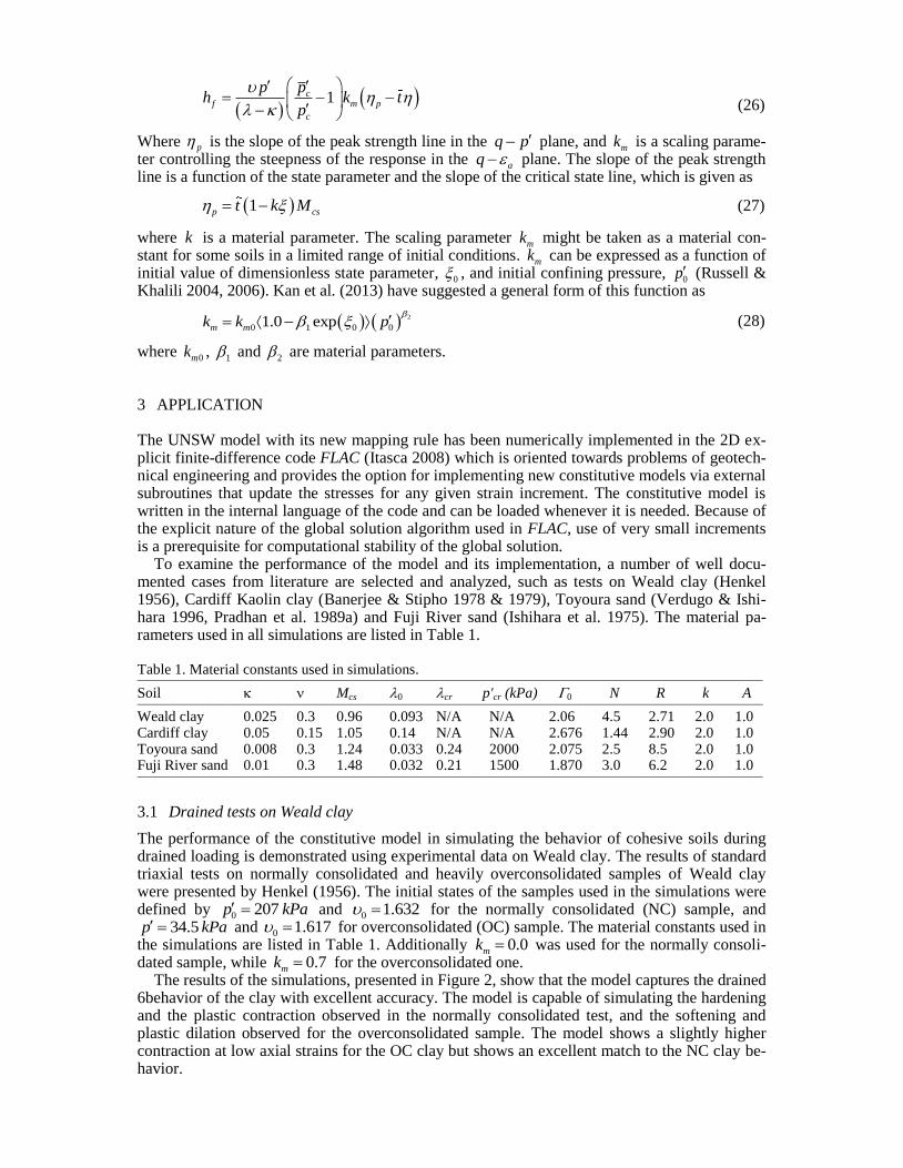
The results of the simulations of drained tests under 0 100p kPa and 500 kPa are shown in Figure 4 and compared with experimental data. While there is a slight discrepancy between the predicted performance and experimental data for the loose sample under the low confining pres-sure, i.e. in test 3, the model predictions for other samples are in excellent agreement with the experimental data.

Figure 4. Drained tests on Toyoura sand.

Figure 5. Undrained tests on Toyoura sand.

The performance and capability of the model to simulate the undrained behavior of sands on a

wide range of initial conditions, including different relative densities and mean effective stress-es, are investigated using 7 undrained tests reported by Verdugo & Ishihara (1996). The out-comes of these simulations are compared with the experimental data in Figure 5 for mean effec-tive stresses vary from 100 to 3000 kPa. In general, the comparison shows satisfactory results, considering the fact that a single set of parameters is used for all simulations under a large range

0

200

400

600

800

1000

1200

0.00 0.05 0.10 0.15 0.20 0.25

De

viat

ori

c St

ress

(kP

a), q

Axial Strain, 1

p'₀=100 kPa, v₀=1.996

p'₀=100 kPa, v₀=1.917

p'₀=100 kPa, v₀=1.831

p'₀=500 kPa, v₀=1.960

p'₀=500 kPa, v₀=1.886

p'₀=500 kPa, v₀=1.810

0.0

0.5

1.0

1.5

2.0

2.5

3.0

1.75 1.80 1.85 1.90 1.95 2.00 2.05

q/p

' 0

Specific Volume,

Experiment (Test 1)

Experiment (Test 2)

Experiment (Test 3)

Experiment (Test 4)

Experiment (Test 5)

Experiment (Test 6)

of confining pressures. Obviously a better fit to the experimental data could have been obtained if a new set of material parameters were used for each test.

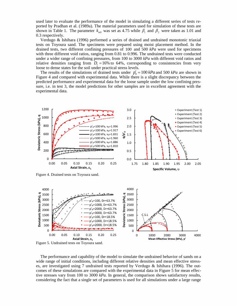
The parameters calibrated from the experiments of Verdugo & Ishihara (1996) are also used to simulate the drained behavior of Toyoura sand reported by Pradhan et al. (1989a). The exper-iments were conducted under various stress paths, including tests to failure under constant axial stress, constant mean effective stress and constant radial pressure, as well as conventional triaxial test (CTC) as shown in Figure 6(a). The parameter 0mk was taken as 1.2 for first time loading and 76.0 for unloading/reloading. 1 and 2 were taken 1.05 and 0.3, respectively.

p

q

p0

5

4

3

2

1

1

3

1

1

1.31

1.51

constanta

constantp

constantstr

31.3 kPa p0 98.1 kPa

01.850)=

01.835)=

01.835)=

01.850)=

01.850)=

(a)

(b)

(c)

Figure 6. (a) Stress paths used for drained tests on Toyoura sand (Pradhan et al. 1989a); (b) & (c) Results of the simulations for different stress paths

The results of simulations are compared with the experimental data in Figure 6(b) & (c). The model captures all features of the soil behavior for different stress paths, with some minor dis-crepancies where the maximum large stress ratio is approached.

3.4 Cyclic drained test on Toyoura sand

Pradhan (1989) and Pradhan et al. (1989b) performed a series of drained triaxial cyclic tests on Toyoura sand. Four cyclic drained tests with constant mean effective stress are selected and used in this study (Kan et al. 2013) among which only one case is presented in this paper due to space limitations. The material parameters obtained from the calibration with the experimental tests conducted by Verdugo and Ishihara (1996) were also used in these simulations. The state pa-rameters and initial conditions of the sample were defined by 0 98.1p kPa and 0 1.855 which represents a very loose sample of Toyoura sand.

Figure 7 shows the results of simulation of a drained cyclic test on this sample under a con-stant mean effective stress and small hysteresis loops of unloading and reloading. The model predicts the main features of the behavior, both in q plane and v q plane. It is worth mentioning that a better match between the results of simulation and the test data could have

been achieved if the model parameters were calibrated for the same test rather than taking as those calibrated for tests performed by Verdugo & Ishihara (1996).

Figure 7. Drained cyclic test on a very loose sample of Toyoura sand with small hysteresis loops.

3.5 Cyclic undrained test on Fuji River sand

Ishihara et al. (1975) conducted a series of undrained triaxial cyclic tests on loose samples of Fuji River sand to study the liquefaction phenomena. Loose samples were obtained by spooning freshly boiled sand into the mold filled with de-aired water. In this paper, one of these tests is selected for simulation to show the performance of the model in capturing the cyclic undrained behavior of granular materials. The material parameters are listed in Table 1 and the initial con-ditions of the sample were taken as 0 156p kPa and 0 1.749. A constant value of mk was used in these simulations due to the limited range of initial state parameters, i.e. a value of km = 2.0 for first time loading and km = 18.0 for unloading/reloading.

Figure 8 presents the results of the undrained test conducted on this sample under irregular cyclic stress amplitude. The predicted behavior is in good agreement with the observed experi-mental data. The model captures the failure of the samples by liquefaction in which the effective normal stress decreases progressively until the stress path reaches the critical state and the mate-rial becomes unstable.

Figure 8. Undrained cyclic test with irregular cyclic amplitude on a loose sample of Fuji River sand.

-1.5

-1.0

-0.5

0.0

0.5

1.0

1.5

2.0

-0.04 -0.02 0.00 0.02 0.04

Stre

ss R

atio

,

Deviatoric Strain, q

Experimental Data

Model Simulation

-0.01

0.00

0.01

0.02

0.03

0.04

-0.04 -0.02 0.00 0.02 0.04

Vo

lum

etr

ic S

trai

n,

v

Deviatoric Strain, q

-200

-150

-100

-50

0

50

100

150

200

250

0 50 100 150 200

De

viat

ori

c St

ress

(kP

a), q

Mean Effective Stress (kPa), p'

C.S.L.

-75

-50

-25

0

25

50

75

100

125

-0.03 -0.02 -0.01 0.00 0.01

De

viat

ori

c St

ress

(kP

a), q

Deviatoric Strain, q

Experimental Data

Model Simulation

4 CONCLUSION

The UNSW bounding surface plasticity model has been proved to be a versatile constitutive model capable of simulating the behavior of clays and sands over a wide range of stresses under drained/undrained and monotonic/cyclic loading conditions. The robustness of the model, im-plemented in FLAC, was demonstrated through simulations of static and cyclic loadings under drained and undrained conditions for different soils. The results of simulations were invariably in excellent agreement with experimental data. The model captures the characteristic features of the behavior of normally consolidated and overconsolidated clays as well as different sands for a wide range of densities and stresses. The stress softening and dilatancy during drained loading of dense sands, liquefaction of loose sands under undrained loading conditions, and the progres-sive stiffening along with hysteresis in the stress-strain relationships for cyclic loading are simu-lated satisfactorily. The versatility of the model in simulation of particular soil was demonstrat-ed using one set of material parameters for all tests conducted by different investigators under different initial conditions.

ACKNOWLEDGEMENTS

The first author is the recipient of the Endeavour Postgraduate Award, Funded by the Australian Government via Department of Education, Employment and Workplace Relations (DEEWR). The support of DEEWR is gratefully acknowledged.

REFERENCES

Banerjee, P., & Stipho, A. 1978. Associated and non‐associated constitutive relations for undrained behaviour of isotropic soft clays. International Journal for Numerical and Analytical Methods in Geomechanics, 2(1), 35-56.

Banerjee, P., & Stipho, A. 1979. An elasto-plastic model for undrained behaviour of heavily overconsolidated clays. International Journal for Numerical and Analytical Methods in Geomechanics, 3(1), 97-103.

Bardet, J. 1986. Bounding surface plasticity model for sands. Journal of Engineering Mechanics, 112(11), 1198-1217.

Been, K., & Jefferies, M. 1985. State parameter for sands. Geotechnique, 35(2), 99-112. Crouch, R. S. 1994. Unified Critical State Bounding Surface Plasticity Model for Soil. Journal of

Engineering Mechanics, 120(11), 2251-2270. Crouch, R. S., & Wolf, J. P. 1994a. Unified 3D critical state bounding surface plasticity model for soils

incorporating continuous plastic loading under cyclic paths. Part II: Calibration and simulations. International Journal for Numerical and Analytical Methods in Geomechanics, 18(11), 759-784.

Crouch, R., & Wolf, J. 1994b. Unified 3D critical state bounding-surface plasticity model for soils incorporating continuous plastic loading under cyclic paths. Part I: constitutive relations. International Journal for Numerical and Analytical Methods in Geomechanics, 18(11), 735-758.

Dafalias, Y., & Popov, E. 1975. A model of nonlinearly hardening materials for complex loading. Acta Mechanica, 21(3), 173-192.

Dafalias, Y.F. & Herrmann, L.R. 1980. A bounding surface soil plasticity model. International Symposium on Soils under Cyclic and Transient Loading, Swansea.

Dowell, M. & Jarratt, P. 1972. The “Pegasus” method for computing the root of an equation. BIT Numerical Mathematics, 12(4), 503-508.

Henkel, D. 1956. The effect of overconsolidation on the behaviour of clays during shear. Geotechnique, 6(4), 139-150.

Ishihara, K., Tatsuoka, F. & Yasuda, S. 1975. Undrained deformation and liquefaction of sand under cyclic stresses. Soils and Foundations, 15(1), 29-44.

Itasca Consulting Group, Inc. 2008. FLAC - Fast Lagrangian Analysis of Continua, Ver. 6.0. Minneapolis: Itasca.

Kan, M.E., Taiebat, H.A. & Khalili, N. 2013. A simplified mapping rule for bounding surface simulation of complex loading paths in granular materials. International journal of Geomechanics, ASCE, Submitted.

Khalili, N., Habte, M., & Valliappan, S. 2005. A bounding surface plasticity model for cyclic loading of granular soils. International journal for numerical methods in engineering, 63(14), 1939-1960.

Khalili, N., Habte, M. & Zargarbashi, S. 2008. A fully coupled flow deformation model for cyclic analysis of unsaturated soils including hydraulic and mechanical hystereses. Computers and Geotechnics, 35(6), 872-889.

Krieg, R. 1975. A practical two surface plasticity theory. Journal of applied mechanics, ASME, 42, 641. Ling, H. I. & Yang, S. 2006. Unified sand model based on the critical state and generalized plasticity.

Journal of Engineering Mechanics, 132(12), 1380-1391. Pastor, M., Zienkiewicz, O. & Chan, A. 1990. Generalized plasticity and the modelling of soil behaviour.

International Journal for Numerical and Analytical Methods in Geomechanics, 14(3), 151-190. Pradhan, T. 1989. The behavior of sand subjected to monotonic and cyclic loadings. PhD thesis, Kyoto

Univ., Japan. Pradhan, T., Tatsuoka, F., Mohri, Y. & Sato, Y. 1989a. An atomated triaxial testing system using a simple

triaxial cell for soils. Soils and Foundations, 29(1), 151-160. Pradhan, T., Tatsuoka, F. & Sato, Y. 1989b. Experimental stress-dilatancy relations of sand subjected to

cyclic loading. Soils and Foundations, 29(1), 45-64. Russell, A.R. & Khalili, N. 2004. A bounding surface plasticity model for sands exhibiting particle

crushing. Canadian Geotechnical Journal, 41(6), 1179-1192. Russell, A. & Khalili, N. 2006. A unified bounding surface plasticity model for unsaturated soils.

International Journal for Numerical and Analytical Methods in Geomechanics, 30(3), 181-212. Sloan, S. W., Abbo, A. J. & Sheng, D. 2001. Refined explicit integration of elastoplastic models with

automatic error control. Engineering Computations, 18(1/2), 121-194. Verdugo, R. & Ishihara, K. 1996. The steady state of sandy soils. Soils and Foundations, 36(2), 81-91.