Application of Probabilistic PCA

RnD Project Report

Submitted in partial fulfillment of requirements for the degree ofBachelor of Technology (Honors)

byAditya Kumar AkashRoll No : 120050046

under the guidance ofProf. Suyash Awate

Department of Computer Science and EngineeringIndian Institute of Technology Bombay

Mumbai 400076, India

April, 2016

Contents

1 Introduction 11.1 Motivation . . . . . . . . . . . . . . . . . . . . . . . . . . . . . . . . . . 2

2 Background 32.1 Factor Analysis Model and Links to PCA . . . . . . . . . . . . . . . . . 3

3 Probabilistic PCA 43.1 The Probability model . . . . . . . . . . . . . . . . . . . . . . . . . . . 43.2 EM method for PPCA . . . . . . . . . . . . . . . . . . . . . . . . . . . 53.3 Properties of MLEs . . . . . . . . . . . . . . . . . . . . . . . . . . . . . 6

4 Missing Data 74.1 PPCA with Missing Data . . . . . . . . . . . . . . . . . . . . . . . . . 74.2 PCA with Missing Data . . . . . . . . . . . . . . . . . . . . . . . . . . 8

5 Experiments 95.1 Dataset . . . . . . . . . . . . . . . . . . . . . . . . . . . . . . . . . . . 95.2 Experiment Design . . . . . . . . . . . . . . . . . . . . . . . . . . . . . 9

6 Results and Observations 116.1 Tobamovirus Data . . . . . . . . . . . . . . . . . . . . . . . . . . . . . 116.2 MNIST Data . . . . . . . . . . . . . . . . . . . . . . . . . . . . . . . . 156.3 USPS Dataset . . . . . . . . . . . . . . . . . . . . . . . . . . . . . . . . 166.4 Binary AlphaDigits Dataset . . . . . . . . . . . . . . . . . . . . . . . . 18

7 Conclusion 19

i

Abstract

Principal Component analysis (PCA) is a classical data analysis technique that findslinear transformations of data that retain the maximal amount of variance. The clas-sical version is not based on a probability model. Researchers have proposed a prob-abilistic model of PCA which is closely related to factor analysis. In this work, weunderstand the Probabilistic PCA (PPCA) and analyse how it handles missing datasituations in which we cannot apply standard PCA. We also try to obtain a comparisionin performance of PPCA with a variant of PCA.

ii

Acknowledgements

I am sincerely indebted to my advisor, Prof. Suyash Awate, IIT Bombay, for his con-stant support and guidance throughout the course of this project. His experience andinsight in the fields of machine learning, image processing and varied aspects of com-puter science in general, was valuable in boosting my interest on this topic.

I finally and especially would like to thank my parents and my whole family for theirsupport and trust in all of my endeavours. The morals they have imparted stayed andwould stay close to me always. I also thank my friends for giving a helping hand duringhard times.

iii

Chapter 1

Introduction

Principal Component analysis (PCA) is a ubiquitous tool for dimensionality reduction.It has many applications data compression, visualization, image processing, exploratorydata analysis, pattern recognition and time series prediction.There are a number of optimization criteria to derive PCA. The most important ofthese is in terms of stardardized linear projection which maximizes the variance in theprojected space [6]. Assume that {yi}, i ∈ {1, 2, ..., n} is a set of d dimensional datavectors. Then the k principal axes {wj}, j ∈ {1, 2, ..., k} are those orthogonal axes ontowhich the retained variance under projection is maximal. It can be shown that wj aregiven by k dominant eigen vectors (those with largest eigen values, λj) of the samplecovariance matrix

S =n∑

i=1

(yi − y)(yi − y)T (1.1)

where y is the sample mean, such that

Swj = λjwj (1.2)

The k principal components of the observed vector yi are given by the vector

xi = WT(yi − y) (1.3)

where W = (w1; w2; ...; wk). The variables xi are uncorrelated such that the covariance

matrix∑n

i=1

xixTi

nis diagonal with elements lambdai.

A complementary property of PCA is that of all the orthogonal linear projections, theprincipal component minimizes the squared reconstruction error. However, PCA doesnot provide a probabilistic model of data. This gives motivation for PPCA.

1

1.1 Motivation

A probabilistic formulation of PCA from a Gaussian latent variable model is obtained.This is closely related to factor analysis. PCA could be viewed a limiting case of such aGaussian model. In such a formulation, the principal axes emerge as maximum likeli-hood parameter estimates. Such a probabilistic formulation is intuitively applealing, asthe definition of a likelihood measure enables comparison with other probabilistic tech-niques, while facilitating statistical testing and permitting the application of Bayesianmethods. Further motivation behind a probabilistic PCA is that it conveys additionalpractical advantage as :

• The probability model offers the potential to extend the scope of conventionalPCA, such as using probabilistic mixtures and PCA projections in missing datacase.

• PPCA can be utilized as a general Gaussian density model. This allows themaximum likelihood estimates for the parameters associated with the covariancematrix to be efficiently computed from the data principal components.

2

Chapter 2

Background

2.1 Factor Analysis Model and Links to PCA

The factor analysis model is a latent variable model which related a d-dimensionalobservation vector y to k-dimensional vector of latent variable x. Following equationexpresses the relationship

y = Wx + µ+ ε (2.1)

where the columns of W, a d× k matrix, are the factors which relate the two vectors,µ allows a non-zero mean and ε is the noise/error.When k < d, the latent variables offer a more parisimonious explanation of the depen-dencies between the observations.The underlying assumptions of x ∼ N (0, I) and ε ∼ N (0,Ψ) induces a correspondingGaussian distribution on observation y ∼ N (µ,WWT + Ψ).The key assumption for the factor analysis model is that, by contraining the error co-variance Ψ to be diagonal, whose elements Ψi are estimated from the data, the observedvariables ti are conditionally independent given the values of latent variables x. Thusthe latent variables are intended to capture the correlation between the observed vari-ables while the error term εi represents the variability unique to particular ti. This iswhere PCA differs from factor analysis, as it treats covariance and variance identically.This distinction in variance and covariance in factor analysis model cause the maximum-likelihood estimates of columns of W to not correspond the the principal subspace ofthe observed data. However, the two methods are linked if we consider a special caseof isptropic error model, where residual variances Ψi = σ2 are constrained to be equal[5].

3

Chapter 3

Probabilistic PCA

3.1 The Probability model

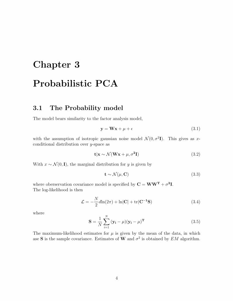
The model bears similarity to the factor analysis model,

y = Wx + µ+ ε (3.1)

with the assumption of isotropic gaussian noise model N (0, σ2I). This gives as x-conditional distribution over y-space as

t|x ∼ N (Wx + µ, σ2I) (3.2)

With x ∼ N (0, I), the marginal distribution for y is given by

t ∼ N (µ,C) (3.3)

where oberservation covariance model is specified by C = WWT + σ2I.The log-likelihood is then

L = −N2dln(2π) + ln|C|+ tr(C−1S) (3.4)

where

S =1

N

N∑i=1

(yi − µ)(yi − µ)T (3.5)

The maximum-likelihood estimates for µ is given by the mean of the data, in whichase S is the sample covariance. Estimates of W and σ2 is obtained by EM algorithm.

4

3.2 EM method for PPCA

In the EM approach to maximize likelihood for PPCA, we consider latent variablesxi to be ’missing’ data and the ’complete’ data to comprise the observations togetherwith latent variables. Corresponding complete log-likelihood is then :

LC =N∑i=1

ln{p(yi,xi)} (3.6)

, where, in PPCA, we get

p(yi,xi) = (2πσ2)−d/2exp{− ||yi −Wxi − µ||

2σ2

}(2π)−k/2exp

{− ||xi||

2

}(3.7)

The posterior is given by

x|y ∼ N (M−1WT(y − µ), σ2M−1) (3.8)

where M = W TW + σ2I. From the appendix B of [1] we obtain following

E-Step :〈xi〉 = M−1WT(yi − µ) (3.9)

〈xixTi 〉 = σ2M−1 + 〈xi〉〈xi〉T (3.10)

M-Step :

W =[∑

i

(yi − µ)〈xi〉][∑

i

〈xixTi 〉]−1

(3.11)

σ2 =1

Nd

∑i

{||yi − µ||2 − 2〈xi〉TWT(yi − µ) + tr(〈xix

Ti 〉WTW)

}(3.12)

The paper [1] shows the combination of both of the above steps rewritten as

W = SW(σ2I + M−1WTSW)−1 (3.13)

σ2 = tr(S− SWM−1WT) (3.14)

S is the sample covariance.Analysis of thes equations show that in normal PCA calculation we require calculationof S which takes O(Nd2) operations. But in case of above EM formulation, we onlyneed to compute SW as

∑i xi(x

Ti W) which takes O(Ndk) operations. Thus when

k � d, considerable computational savings would be obtained. This is one of thebenefits of using the EM version of PPCA.

5

3.3 Properties of MLEs

In paper [1] it is shown that with C = WWT + σ2I, likelihood 3.6 is maximized when

WML = Uk(Λk − σ2I)1/2R (3.15)

where k column vectors in Uk are the principal eigenvectors of S, with correspondingeigenvalues in Λk, and R is arbitary orthogonal rotation matrix.When W = WML, MLE for σ2 is

σ2ML =

1

d− k

d∑j=k+1

λj (3.16)

which has interpretation of variance lost in projection, averaged over the lostdimension. Using this we can see how this lost variance is subtracted from the eigenvectors in the estimation of WML.

6

Chapter 4

Missing Data

4.1 PPCA with Missing Data

One of the motivation of using PPCA is that it provides interpretation to the datathat is missing from the observation variable. Such missing data variables are assumedto be ’parameters’ in the model and a generic EM algorithm is designed to handle thecase.An example of missing data case would be in computer vision field, when we model adodecahedran from a sequence of segmented images. One sample of data would containonly information (in form of normals) for only 6 of the faces, while rest is missing data.

In these cases the E-step of EM algorithm is generalized to following :Generalized E-step [2]

• If y is incomplete, then we find a unique pair of points x∗,y∗ (such that x∗ lies inthe current principal subspace and y∗ lies in the subspace defined by the knowninformation about y) which minimize the norm ||Wx∗ − y∗ + µ||2. Now we setthe corresponding expectation of x to x∗ and correspoinding observed variabley to y∗. The solution is obtained by finding solution to a particular constrainedmatrix.

• If y is complete, then 〈x〉 is found as before.

The above steps emerge as a result of treating the missing values as parameters tothe model. The optimization problem results from maximizing the likelihood of thecomplete data.

7

4.2 PCA with Missing Data

In this work we also try to compare following PCA modification for missing data.

• PCA with reference to Factor analysis : In this approach we try to estimatethe missing values using the minimization of ||Wx∗ − y∗ + µ||2. x is the latentvariable. In each iteration, first y is estimated using this minimization, then W isestimated by finding k principal component of covariance of Y. The optimizationproblem emerges as a result of assuming the data generation model for y basedon the factor model.

• Standard PCA with missing values filled by mean : This case is basedon direct estimation of missing values by assuming Gassian model for the data.We assume observation having mean µ and covariance S. If there was no miss-ing value, the estimation of mean and covariance would be sample mean andcovariance. Now with missing data being there, we first estimate mean to besample mean of data which is present. The missing data then obtained by takingderivative comes out to be the components from mean. Thus in the next step,taking the mean over entire data does not change it. Effectively in this methodwe replace the missing data with the mean of the non-missing data.

8

Chapter 5

Experiments

We give examples to show how PPCA can be exploited for practical examples. Theexperiments focus on the application of PPCA to the dataset with missing values.

5.1 Dataset

We use following dataset :

1. Tobamovirus dataset : 38 virus , each with 18 features

2. MNIST dataset : The MNIST database of handwritten digits has a trainingset of 60,000 examples, and a test set of 10,000 examples. The digits have beensize-normalized and centered in a fixed-size image of 28×28 pixels.

3. USPS dataset : Handwritten Digits, 8-bit grayscale images of ”0” through ”9”;1100 examples of each class.

4. Binary Alphadigits : Binary 20x16 digits of ”0” through ”9” and capital ”A”through ”Z”. 39 examples of each class.

5.2 Experiment Design

• For the Tobamovirus dataset, the data is projected into 2 dimensions for thepurpose of visualization of dimension reduction by PCA and PPCA. The datasetis claimed to have three sub-groups. The missing data is simulated by randomlyremoving each value in the dataset with probability 20%. The aim is to find howmuch of the sub-groups is being preserved.

• For the handwritten digits datasets, the data was randomly divided intp 7:3 ratiofor training and testing, in case the two sets are not present.

9

We train a classifier based on mahalanobis distance. For each digit a factormatrix (W) is obtained using PCA/PPCA on the training data. Based on thefactor matrix, we find the projections of all the training data points. Mahanalobisdistance of each test data sample is calculated in latent dimension from the train-ing set of each digit. The digit which gives least distance is predicted as the label.

For missing data case, the factor matrix and latent variables are learnt fromtraining data having missing values. The missing values are simulated by ran-domly removing the data with a given probability. The prediction is done usingthese learnt values. The algorithms are analysed for different amount of missingvalues.

With this experiment, we try to find the behaviour (prediction accuracy) of eachof the algorithms with different amount of training data.

10

Chapter 6

Results and Observations

6.1 Tobamovirus Data

For the Tobamovirus data we can see that the projection 6.1 of the complete dataobtained using standard PCA gives three sub-groups. Then we have 6.2 which is theprojection obtained using PPCA closed form given in []. Figure 6.3 is the projectionobtained by the PPCA run with EM algorithm. The projection is the same except forbeing rotated about some point. The roation is dependent on the initialization of thealgorithm.

For the missing data case (20% missing), it is clear that both figure 6.4 and 6.5 isable to obtain three sub-grounps. The salient features of the projection is clear, evenwhen all data points have suffered from at least one missing value. Both the algorithmsseems to perform equally good in this dataset.

11

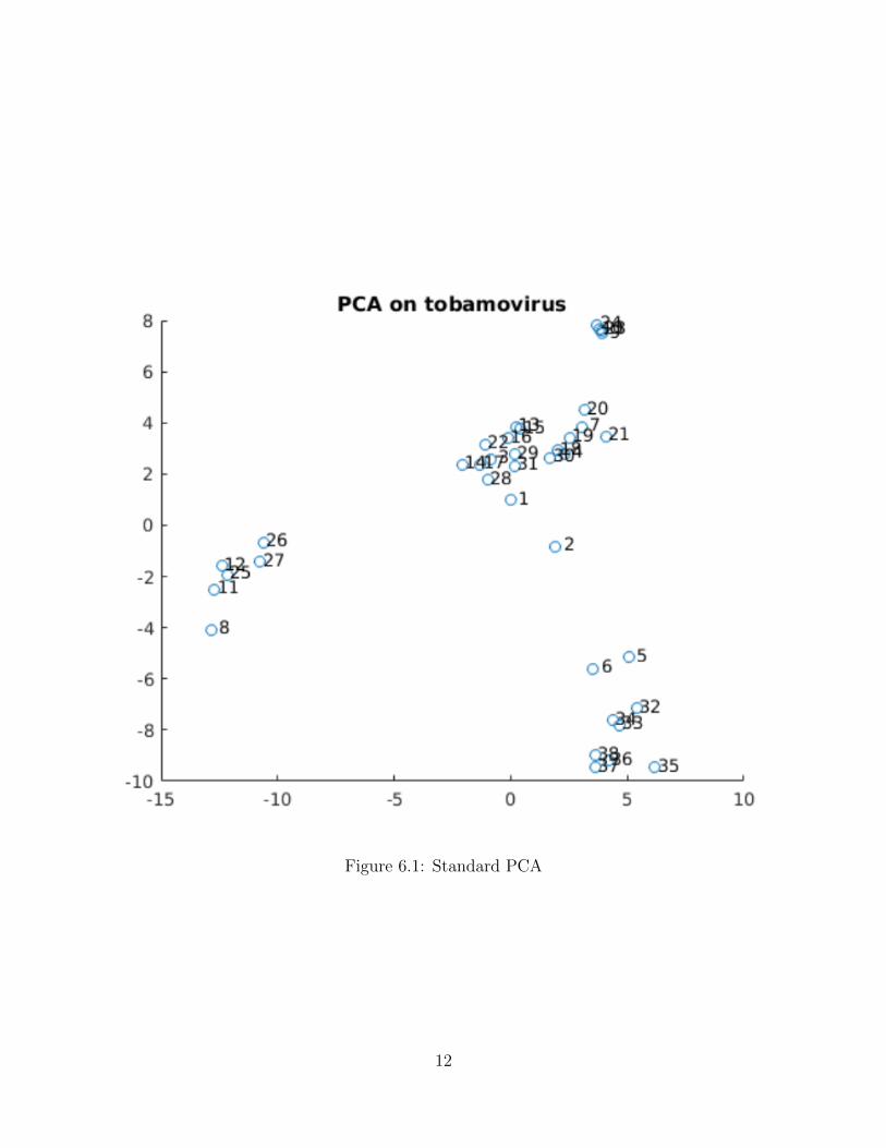
Figure 6.1: Standard PCA

12

Figure 6.2: PPCA using closed form formula

Figure 6.3: PPCA using EM algorithm

13

Figure 6.4: PPCA projection with 20% missing data using EM

Figure 6.5: PCA projection with 20% missing data

14

Figure 6.6: Accuracy vs latent dimension for MNIST

6.2 MNIST Data

MNIST data contains 28× 28 images. Each images contains a handwritten digit. Thetask is predition of the digits. The experiment design outlines in the last chapter isfollowed.

The plot 6.6 shows how the accuracy increases rapidly at start but then becomesstatic. The latent dimension k = 133 is a good choice as it has highest accuracy in theregion plotted and also the increase becomes very less after that point.

The experiments that follow have k = 133 fixed. Following is the table showingaccuracy of PPCA with missing values and comparision with other variants PCA forhandling missing data.

15

Missing Data % Accuracy forPPCA with EM

Accuracy forPCA based onFactor Model

Accuracy forPCA based on µfor missing value

0 88.01 87.97 87.971 88.25 88.27 88.405 89.62 91.19 90.3020 92.74 93.08 93.0140 92.44 71.71 93.0560 83.49 2.81 91.4480 - - 86.3190 - - 78.0899 - - 42.94

Table 6.1: Accuracy for Missing data

From table 6.1, we can find following observations

1. The accuracy increase with increase in missing data till a certain fraction. Aftera threshold the accuracy drops.

2. The accuracy of PCA handling missing data based on factor model drops sig-nificantly (Column 2). The possible explanation for this is that the number ofunknowns in the minimization problem ||y −Wx− µ|| becomes large as x is la-tent and y also has missing data. So the system of equations gives poor estimatesof the missing data.

3. PCA based on missing data filled by µ components show the best acuracy formissing data. A possible explanation is that a large part of data is a backgroundimage and digits occupy only lesser fraction. So larger number of missing dataare estimated correclty using mean which would be towards background pixelside.

6.3 USPS Dataset

USPS also contains handwritten digit images. The experiment outlined for MNIST isperformd again for USPS. For each experiment data is randomly divided into 7 : 3ratio for training and testing. From figure 6.7, it can be seen tha k = 100 is an idealchoice for the latent dimension. Further experiments keep k = 100. We can also seesimilar behaviour of this data set as the MNIST. Table 6.2 also contain the accuracyon conplete data as last column as the data partitioning is random.

16

Figure 6.7: Accuracy vs latent dimension for USPS

Missing Data % Accuracy forPPCA with EM

Accuracy forPCA based onFactor Model

Accuracy forPCA based on µfor missing value

Accuracy Stan-dard PCA oncomplete data

0.5 89.96 89.57 90.12 89.421 89.93 89.72 89.84 88.845 90.51 90.54 91.90 88.3610 91.87 91.60 93.36 89.3920 92.30 92.48 93.87 90.3940 83.69 84.63 91.51 88.3060 55.21 52.30 88.75 88.60

Table 6.2: Accuracy for Missing data for USPS

17

Figure 6.8: Accuracy vs latent dimension for Alpha digits

6.4 Binary AlphaDigits Dataset

The data is present in form of 39 samples for each 36 classes. Each sample is a 20× 16image. Since the amount of data present is low picking up a large latent dimension isnot feasible for calculating the mahalanobis distance.

From the plot 6.8, it is clear that the accuracy increases till the number of latentdimension k reaches the number of training sample (k ∼ 40). After that the accuracydoes not increase. This makes this dataset difficult to analyse. We donot any furtherprediction analysis for this dataset.

18

Chapter 7

Conclusion

In this work, we see how principal component analysis model can be viewed as a max-imum likelihood procedure based on a probability density model of the observed data.We also see links to PPCA to factor analysis and subtle difference between the two,as well as the underlying assumption for PPCA. An EM algorithm was discussed forPPCA which iteratively maximized the likelihood of the data.

The main aim of this work was understanding PPCA and its application on real worlddataset. We apply PPCA to the case of missing data and compare its performancewith different version of PCA made to handle missing data. In the Results chapter wesee how PPCA is capable of handling missing data along with providing a reasonablemodel for interpretation of the results. But we found out that for the datasets whichwe covered PCA with missing data replaced by mean of non-missing data gives bestperformance. This leads us to conclude that for cases where data is not generated us-ing mixtures of gaussian, the sophistication of PPCA is only to provide a probabilistictouch to the classical version of PCA.The importance for EM algorithm of PPCA is more when the data has an inherentmixture model distribution. In such cases, PCA cannot trivially handle it. But PPCAcould easily incorporate it into the model and handle such cases.

19

Bibliography

[1] Tipping, Michael E., and Christopher M. Bishop. ”Probabilistic principal com-ponent analysis.” Journal of the Royal Statistical Society: Series B (StatisticalMethodology) 61.3 (1999): 611-622.

[2] Roweis, Sam. ”EM algorithms for PCA and SPCA.” Advances in neural informationprocessing systems (1998): 626-632.

[3] Chen, Haifeng. ”Principal component analysis with missing data and outliers.”http://www.cmlab.csie.ntu.edu.tw/~cyy/learning/papers/PCA_Tutorial.

pdf (2002).

[4] LeCun, Yann, Corinna Cortes, and Christopher JC Burges. ”The MNIST databaseof handwritten digits.” (1998).

[5] Whittle, Peter. ”On principal components and least square methods of factor anal-ysis.” Scandinavian Actuarial Journal 1952.3-4 (1952): 223-239.

[6] Hotelling, Harold. ”Analysis of a complex of statistical variables into principalcomponents.” Journal of educational psychology 24.6 (1933): 417.

20