APPLICATION OF OBSTACLE DETECTION AND PHOTO

RECOGNITION FOR USE IN AUTONOMOUS VEHCLES

A THESIS

Presented to the University Honors Program

California State University, Long Beach

In Partial Fulfillment

of the Requirements for the

University Honors Program Certificate

Daniel Lee

Spring 2018

ABSTRACT

APPLICATION OF OBSTACLE DETECTION AND PHOTO RECOGNITION FOR USE IN

AUTONOMOUS VEHCLES

By

Daniel Lee

May 2018

Autonomous cars are still prone to accidents on the open road due to the inaccuracies

present in current generation sensing technology. The aim of this research is to improve the

obstacle detection capabilities of these unmanned vehicles. This thesis will focus primarily on

the implementation of a real-time object detection program with object recognition capabilities

using open source computer vision and machine learning libraries to assist in improving the

quality of detection. We propose multiple solutions using three different techniques: 1) RGB to

HSV thresholding to accurately detect an object in a frame, 2) Selective search to accurately

detect multiple objects in a frame, and 3) Object classification through a neural network. The

results showed that the selective search algorithm offered the most accurate way to detect

obstacles.

iii

ACKNOWLEDGEMENTS

Thank you to Dr. Oscar Morales-Ponce for allowing me to join his lab, it has been a joy

to work on such a fun project.

I also want to thank Kashima, Lizette, Jacqueline, and Vincent for all of their support

throughout these past 4 years as I would not have arrived at this point without them.

Lastly, I want to thank my friends and family for encouraging me to continue pursuing

the honors program and to finish my thesis.

iv

TABLE OF CONTENTS

Page

ACKNOWLEDGEMENTS ................................................................................................... iii

LIST OF TABLES ................................................................................................................. v

LIST OF FIGURES ............................................................................................................... vi

CHAPTER

1. INTRODUCTION ..................................................................................................... 1

Hardware Used............................................................................................... 2

Software Used ................................................................................................ 5

2. LITERATURE REVIEW .......................................................................................... 6

3. METHODS ................................................................................................................ 10

HSV Thresholding ......................................................................................... 10

Selective Search ............................................................................................. 12

TensorFlow Image Recognition ..................................................................... 15

4. RESULTS .................................................................................................................. 16

5. CONCLUSION .......................................................................................................... 20

REFERENCES ...................................................................................................................... 21

v

LIST OF TABLES

TABLE Page

1. RealSense Video Resolutions of RGB and Depth Sensors ........................................ 3

vi

LIST OF FIGURES

FIGURE Page

1. A breakdown of the RealSense camera and the images it can produce ..................... 3

2. A top down view of the NVIDIA Jetson TX2 Development Board .......................... 4

3. The HSV color model ................................................................................................ 10

4. The original image (left) and the thresholded image (right) ...................................... 11

5. A thresholded image of a ball .................................................................................... 12

6. The input image (left) and the over-segmented image (right) ................................... 13

7. Grouping adjacent segments (left) and the final output (right) .................................. 14

8. A full example of the selective search algorithm being performed ........................... 15

9. Input image (above) and the resulting probabilities list (below) ............................... 16

10. Input image (left) and thresholded output (right) ...................................................... 17

11. Input image (above) and the output (below) after applying the selective search

algorithm ........................................................................................................... 18

1

INTRODUCTION

According to the Association for Safe International Road Travel (ASIRT), nearly 1.3

million fatal car accidents occur every year globally, averaging 3,287 deaths per day. Almost

37,000 of those deaths occur within the US and are considered to be one of the greatest annual

causes of death (8). To combat this growing epidemic, companies such as Google, Uber, and

Tesla have poured millions of dollars into researching techniques to provide accurate obstacle

detection for self-driving vehicles. Each of these companies have released several autonomous

vehicles and have been training the automobiles under different conditions to improve their

detection capabilities. However, even with state of the art technology and years of training, many

of these companies have been under public scrutiny due to fatal accidents caused by these

unmanned vehicles. For example, NBC News recently released a report on an autonomous car

created by Uber hitting and killing a pedestrian in Arizona. NBC also reported that the car would

regularly violate other traffic ordinances, such as cutting through bicycle lanes (4). The LA

Times also reported that a Tesla semiautonomous car hit a freeway barrier, caught fire, and

ultimately killed the occupant of the vehicle (7).

With autonomous cars still in their infancy and prone to accidents, this project aims to

help further the research into techniques for detecting obstacles accurately. Though this research

may only contribute a small change in the betterment of self-driving vehicles, even reducing the

amount of fatal accidents would be a step in the right direction. This project will primarily focus

on the obstacle detection and classification portion of an autonomous vehicle. This will be

accomplished through the use of a 3D camera and other special hardware, which will help

improve detection rates and process video streams in real time. Specifically, this research aims to

2

implement a real-time object detection program with object recognition capabilities using open

source computer vision and machine learning libraries for use in autonomous vehicles. This

implementation will also have the potential to be built upon so that integration of other

technologies, such as lane detection and surface detectors, will be possible. The three techniques

explored in this paper will help to achieve this goal.

The remaining portion of Chapter 1 will explain the specific hardware and software used

for obstacle detection and photo recognition. Chapter 2 delves into other literature and the

reasoning behind the techniques chosen in this project. Chapter 3 focuses on the three techniques

chosen for this research to achieve the goal of this project, and Chapter 4 discusses the results of

those techniques. Finally, Chapter 5 explains future work and the final conclusions of this

project.

Hardware Used

For this system, an Intel© RealSense™ R200 3D Camera (RealSense) was used to stream

data and an NVIDIA Jetson TX2 Development Board (Jetson) was used to process the image

stream and output the final regions. The RealSense is a USB device comprised of two

stereoscopic infrared (IR) cameras used for depth perception and a single RGB camera used for

color as seen in Figure 1.

3

FIGURE 1: A breakdown of the RealSense camera and the images it can produce. Photo

provided by Intel© Developer Zone.

An IR laser projector is also included for 3D scanning capabilities for use in scene recreation or

character modeling. The RealSense is capable of providing video streams at differing framerates

TABLE 1. RealSense Video Resolutions of RGB and Depth Sensors

Camera

Frames per

Second (FPS) Pixel Density Camera Pixel Density

Depth 60 320x240 RGB 640x480

Depth 60 480x360 RGB 320x240

640x480

Depth 30 320x240 RGB 640x480

1920x1080

Depth 30 480x360 RGB

320x240

640x480

1920x1080

Note: Data provided by Intel© Developer Zone.

4

and resolutions, where the most common settings are listed in Table 1. When streaming video

data, the RealSense camera has a maximum range of 10 meters when used outside, and a range

between 0.5 – 3.5 meters when used inside. All methods and tests performed on the system using

this camera have been done indoors.

In conjunction with the RealSense camera, the Jetson was used primarily to process both

RGB and depth data streams. The reason why this particular board was chosen was for its CUDA

architecture, which is a proprietary computing platform that allows for parallelism in high

performance computing. Simply put, this board was equipped with a GPU that allowed for a

workload to be split amongst many cores. This aided in speeding up the capabilities of creating

bounding boxes around obstacles in real-time and to improve the speed of the Tensorflow

library.

FIGURE 2: A top down view of the NVIDIA Jetson TX2 Development Board. Photo provided

by Hackaday.

5

Software Used

In order to utilize the RealSense camera, Intel provided an open source library named

librealsense. This library included camera capture functionality, which allowed for me to stream

RGB and depth video data into the Jetson for processing. The second library, OpenCV, included

packages to manipulate the data streamed from the RealSense camera. The software is

prepackaged with functions to manipulate RGB pixel data and algorithms to aid with object

detection. The library was also designed to take advantage of multi-core processing, which is

possible on the Jetson, and is computationally efficient enough to work in real-time applications.

The third piece of software used was Tensorflow, which is a machine learning library that

focuses on visual recognition tasks. Data processed from the RealSense is sent to the Tensorflow

library to classify detected obstacles.

6

LITERATURE REVIEW

In order to accomplish my goal to implement a real-time obstacle detection and photo

recognition system, I first looked into different types of sensors available. Han, Li, Liao, Wang,

and Zhang (6) proposed a real time obstacle detection system based on a Lidar and a wireless

sensor. A Lidar is a 3 dimensional 3D radar which scans an area and returns a point map of

detected surfaces. The team primarily used the Lidar as the object detector, where 64 laser beams

with a max range of 120m rotate 360 degrees to scan the room around it. The collected data is

then assembled into a grid map and is converted to an obstacle prescheme and is compared

against measurements taken by the wireless sensor. The sensor is capable of measuring an

objects size, speed, and direction and uses this information, along with the generated obstacle

prescheme, and performs a consistency test. If correct and all data is valid, the system updates

the model and creates a bounding box, claiming that it is an obstacle.

Although the Lidar had all of the tools for scanning and detecting obstacles, I

unfortunately was unable to obtain one at the beginning of my research. I also did not have

access to a wireless sensor that could detect size, speed, and direction.

This led to me to explore other options, such as the system presented by Fu, Qiu, Song,

Wang, and Yi (5) that aimed to detect near obstacles using a stereo camera and far obstacles

using a millimeter wave (mmw)-radar while simultaneously classifying the detected objects.

These objects would be detected using a region of interest (ROI) detection module and by

employing the use of a stereo images matching algorithm. The original images are first gray-

scaled and a UV-disparity map is created, which is a color segmented image depicting the

proximity of detected obstacles. These obstacles will be highlighted, ranging from red as being

7

the closest and blue being the farthest. This disparity map is then fed through the obstacles

classifier module and the detected modules are then classified as either a danger, potential

danger, or non danger.

The gray-scaling idea behind this research helped me to develop the idea for first

technique for my project and the fact that the team used a stereo camera set me on the path to use

the RealSense camera. Instead of just using the stereo camera to detect close objects, I sought to

detect far objects as well without the use of the mmw-radar, which led me to the system created

by Bertozzi, Bombini, Cerri, Medici, Antonello, and Miglietta (2). The team proposed a system

that would detect and classify road obstacles through the use of a camera, radar, and an inertial

sensor. The radar is able to measure the speed and distance of nearby objects but relies on the

camera to provide enough data points to detect obstacle boundaries. Software wise, the team

implemented two algorithms: one to detect vehicles and one to detect pedestrians. The vehicle

detection algorithm accepts radar data for distance from the object and vision data for position

and width of the object and locates areas of interest within the input images. The images are

thresholded (unneeded pixels are darkened and needed pixels are lightened) and the areas of

interest are scanned for both vertical and horizontal symmetry to a pre-computed set of data. The

edges of the potential correct areas of interest are then marked with bounding boxes, and the

multiple boxes are resampled, mixed, and filtered to delete false detection areas. The final output

is a bounding box surrounding the detected vehicle.

In the pedestrian detection algorithm, input data from both the radar and vision sensors

are taken in and the resulting images are compared against preset data that strongly suggest

symmetry of that of a pedestrian. Unlike vehicle detection, images of pedestrians have strong

8

edges when compared to the background of an image, making this a specific characteristic to

look out for when determining regions of interest.

This system helped me to further develop my first technique by thresholding needed

pixels to white and unneeded pixels to black, along with giving me the idea to add bounding

boxes to point out regions of interest in an image. Studying this paper also gave me insight into

how to implement the photo recognition portion of my project, as this system would classify a

pedestrian according to previous models, similar to that of a neural network. The issue here is

that this paper presents the use of a radar for depth measurements. The RealSense camera that I

had chosen to use avoided this flaw with the included ability to stream depth data.

The next paper solidified my choice in just using a camera through the system proposed

by Bertozzi and Broggi (3). The GOLD (Generic Object and Lane Detection) system is an

architecture that can be used in autonomous vehicles and the implementation of this system relies

solely on visual data collected from standard cameras and does not rely on radars. GOLD

provides two main functions: lane detection guided by existing, painted lines on a road and

obstacle detection, relying on an optical flow approach.

In the lane detection algorithm, images streamed from the camera are processed and the

pixel data is compared against those of painted lane markings. Both color data and edge

detection are then used to infer potential regions of interest. Bounding boxes are then applied to

the areas of interest.

In the obstacle detection algorithm, the GOLD team opted to use the optical flow

approach. This method requires an input of at two stereo images and processes them using two

steps: motion estimation of the camera (ego-motion) is calculated first, then obstacles are

9

detected through the analysis of the differences between the expected and real velocity field.

The methods provided in the paper shows that using only a camera is possible in creating

an accurate obstacle detection technique.

Ayash, Cohen, Fetaya, Garnett, Goldner, Horn, Levi, Oron, Silberstein, and Verner (1)

proposed an efficient and unified system that would detect obstacles using two methods: camera-

based detection and column-based detection. This system would also rely on a deep,

convolutional neural network to improve positive detection rates among datasets. The team’s

work is based on a pre-existing system known as StixelNet, which is another obstacle detection

framework. In this specific implementation, the team focused on using two algorithms: one to

detect a bottom contour of an object and another to detect columns without any obstacles. These

two algorithms are inputted with data from a 3D point cloud gathered from stereo cameras and a

Lidar, where the data is separated into multiple clusters. Once processed the algorithms produce

a bounding box overlay, coloring different detected objects with distinct colors.

After reviewing several papers on obstacle detection, I came to the conclusion that using

a 3D camera was the best way to move forward. A Lidar would have been too costly to obtain,

and a other wireless sensors simply were not available for purchase. The methods used within

these papers also guided me in attempting to test three different techniques for obstacle detection

and photo recognition.

10

METHODS

In order to accomplish my goal of implementing a real-time object detection program

with object recognition capabilities, I used three different methods, the first two for obstacle

detection and the third for image recognition. The first method detects obstacles through the

conversion of RGB data to HSV values and thresholding the image to a binary black or white

image. The second method detects obstacles through the use of the selective search algorithm.

The third method classifies objects using the open source library TensorFlow.

RGB to HSV Conversion

Expanding upon the first technique to detect obstacles, I converted RGB pixel data from

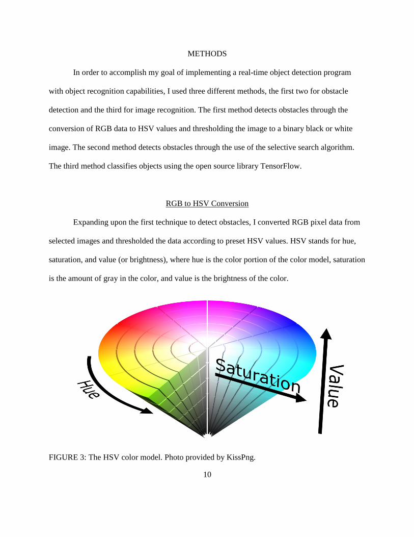
selected images and thresholded the data according to preset HSV values. HSV stands for hue,

saturation, and value (or brightness), where hue is the color portion of the color model, saturation

is the amount of gray in the color, and value is the brightness of the color.

FIGURE 3: The HSV color model. Photo provided by KissPng.

11

The hue value ranges from 0 to 179, where each step represents a color ranging from red, yellow,

green, cyan, blue, and magenta. The saturation value ranges from 0 to 255, where 0 introduces

the most amount of gray to a color while 255 adds no gray to the primary color. The brightness

value ranges from 0 to 255, where 0 adds no intensity to the image and 255 reveals the most

color.

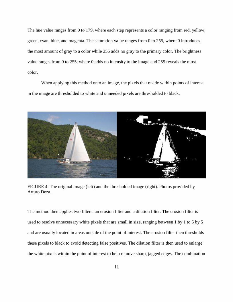
When applying this method onto an image, the pixels that reside within points of interest

in the image are thresholded to white and unneeded pixels are thresholded to black.

FIGURE 4: The original image (left) and the thresholded image (right). Photos provided by

Arturo Deza.

The method then applies two filters: an erosion filter and a dilation filter. The erosion filter is

used to resolve unnecessary white pixels that are small in size, ranging between 1 by 1 to 5 by 5

and are usually located in areas outside of the point of interest. The erosion filter then thresholds

these pixels to black to avoid detecting false positives. The dilation filter is then used to enlarge

the white pixels within the point of interest to help remove sharp, jagged edges. The combination

12

of the two removes unnecessary noise within the image and the resulting output should only have

a large area of white with little to no noise surrounding it. A bounding box is then drawn above

the points in white to indicate the detection of an obstacle.

FIGURE 5: A thresholded image of a ball. The point of interest is surrounded by a bounding

box. Photo provided by StackOverflow.

Selective Search

Expanding upon the second technique to detect obstacles, I used the selective search

algorithm, which is provided within OpenCV, for object detection. The algorithm works using

13

the following steps:

• It first takes an image and performs an over-segmentation of the image based on the

intensity of the pixels using the Felzenszwalb-Huttenlocher segmentation method,

separating different regions of the photo with different colors.

• 2) The image is then analyzed and different regions are grouped together based on

similarities.

• 3) Step two is repeated multiple times to combine more color groups with each pass.

• 4) Bounding boxes are outputted on top of the original image based on the color

separated groups.

FIGURE 6: The input image (left) and the over-segmented image (right). The input image has

only been over-segmented by the algorithm and no grouping has been applied. Photo provided

by Big Vision, LLC.

In the first step, the image is over-segmented, meaning that the algorithm looks for distinctive

edges along the input image and shades the two segments with different colors. This first step is

not an accurate representation of what objects are located in the photo but does provide a map of

14

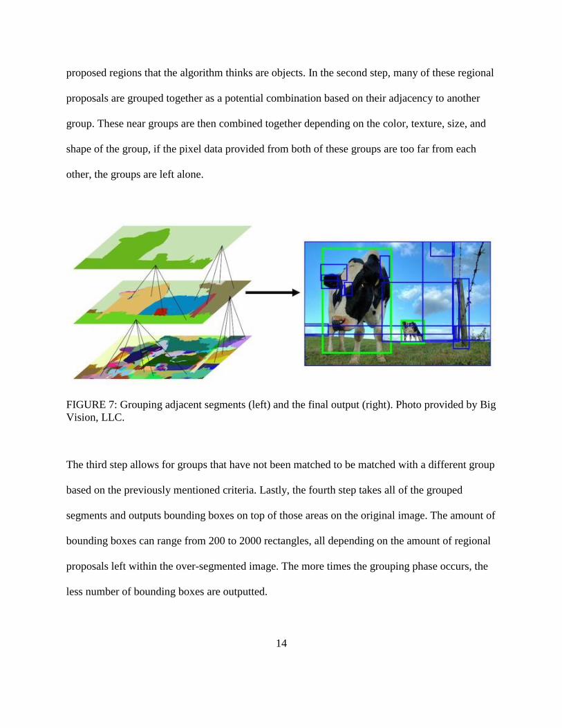
proposed regions that the algorithm thinks are objects. In the second step, many of these regional

proposals are grouped together as a potential combination based on their adjacency to another

group. These near groups are then combined together depending on the color, texture, size, and

shape of the group, if the pixel data provided from both of these groups are too far from each

other, the groups are left alone.

FIGURE 7: Grouping adjacent segments (left) and the final output (right). Photo provided by Big

Vision, LLC.

The third step allows for groups that have not been matched to be matched with a different group

based on the previously mentioned criteria. Lastly, the fourth step takes all of the grouped

segments and outputs bounding boxes on top of those areas on the original image. The amount of

bounding boxes can range from 200 to 2000 rectangles, all depending on the amount of regional

proposals left within the over-segmented image. The more times the grouping phase occurs, the

less number of bounding boxes are outputted.

15

FIGURE 8: A full example of the selective search algorithm being performed. Photo provided by

SemanticScholar.

Tensorflow

Expanding on the third technique, I used Tensorflow, which is an open source machine

learning library, for photo recognition. The particular model that I used is called Inception-v3, a

deep convolutional neural network that was trained particularly to aid in visual recognition tasks.

After running either one of the first two techniques explained above, the program would cut a

region out from the resulting bounding boxes and stream it into Tensorflow, where the model

would then return a list of probabilities of what the object in the image is. The highest probability

would be automatically taken and printed out to show a successful run of both the obstacle

detection and image recognition portions of the project.

16

FIGURE 9: Input image (above) and the resulting probabilities list (below). Photos provided by

Wikipedia and Tensorflow.

17

RESULTS

After applying the RGB to HSV thresholding method, I observed that a singular object

could be detected depending on the preset HSV values in real time. Although the test was

successful in detecting the region that I wanted, it was unable to detect any other object of a

different color. I realized that this method would not suffice for the detection of multiple objects

because of how the bounding box would expand to encapsulate the edges of multiple points of

interest.

FIGURE 10: Input image (left) and thresholded output (right). The HSV values were preset to

detect black for this particular run.

This led to the adoption of the selective search algorithm early on into the project, which

provided more accurate results. I observed that the algorithm was able to correctly identify

multiple objects in a scene when the input image was passed through multiple times. Though

there were some false positive regional proposals, the accuracy of the algorithm was unmatched

to the first technique used. However, the high accuracy of the algorithm was coupled with slow

18

processing times. The algorithm was not able to keep up with the video stream, which outputted

30 frames per second, and could only process around 5 frames per second.

FIGURE 11: Input image (above) and the output (below) after applying the selective search

algorithm. Only the first 20 bounding boxes were printed from the hundreds generated.

19

Lastly, I was unable to obtain quality data for the image recognition portion of my research. The

original data that was outputted by the neural network did not meet my quality criteria, which

had to be at least a 70% assurance that the object in the image was actually what it was supposed

to be. The list outputted by Tensorflow did not contain any value above 50%, and the highest

result usually was inaccurate. A possible issue that may have caused this inaccuracy could be

that the images cut from the bounding boxes had backgrounds that were too noisy, meaning that

there were too many other distinctive features that would have been detected by Tensorflow.

Another issue with the program was the long processing time, on average it took around 5

seconds per image inserted to obtain a probability list.

20

CONCLUSION

Taking into account the results from my research, I believe that this project has provided

a base for future implementations of autonomous vehicle research. The first technique explored,

RGB to HSV thresholding, successfully allowed for real-time detection of singular objects

within a certain color space. The second technique, selective search, successfully detected

multiple objects in a scene. Finally, the third technique for photo recognition showed promise in

successfully classifying objects, but will need to be tweaked. In the future, I would like to

improve the speed of the amount of bounding boxes drawn on top of an input image using the

selective search algorithm. This would allow for the obstacle detection portion of my research to

run in real-time at 30 frames per second, instead of 3 to 5 frames per second. I also would like to

combine the photo recognition portion and the object detection portion into one program once

more valid results are outputted from the photo classification part of the project.

21

REFERENCES

(1) Ayash, A., Cohen, R., Fetaya, E., Garnett, N., Goldner, V., Horn, K., Levi, D., Oron, S.,

Silberstein, S., Verner, U. (2017). Real-time category-based and general obstacle

detection for autonomous driving. IEEE Xplore Digital Library.

(2) Bertozzi, M., Bombini, L., Cerri, P., Medici, P., Antonello, P. C., Miglietta, M. (2008).

Obstacle Detection and Classification fusing Radar and Vision. IEEE Xplore Digital

Library.

(3) Bertozzi, M., Broggi, A. (1998). GOLD: A Parallel Real-Time Stereo Vision System for

Generic Obstacle and Lane Detection. IEEE Xplore Digital Library.

(4) Eisenstein, P. A., (2018). Fatal crash could pull plug on autonomous vehicle testing on

public roads. Retrieved from www.nbcnews.com.

(5) Fu, M., Qiu, F., Song, W., Wang, M., Yi, Y. (2018). Real-Time Obstacles Detection and

Status Classification for Collision Warning in a Vehicle Active Safety System. IEEE

Xplore Digital Library.

(6) Han, J., Li, P., Liao, Y., Wang, S., Zhang, J. (2018). Real Time Obstacle Detection

Method Based on Lidar and Wireless Sensor. IEEE Xplore Digital Library.

(7) Hiltzik, M., (2018). Self-driving car deaths raise the question: Is society ready for us to

take our hands off the wheel?. Retrieved from http://www.latimes.com.

(8) Nearly 1.3 million people die in road crashes each year. (2018). Road Crash Statistics.

Retrieved from http://asirt.org.