Application of Numerical Analysis to Root Locus Design of ...
59
Portland State University Portland State University PDXScholar PDXScholar Dissertations and Theses Dissertations and Theses 2-25-1972 Application of Numerical Analysis to Root Locus Application of Numerical Analysis to Root Locus Design of Feedback Control Systems Design of Feedback Control Systems Steve William Justice Portland State University Follow this and additional works at: https://pdxscholar.library.pdx.edu/open_access_etds Part of the Electrical and Computer Engineering Commons Let us know how access to this document benefits you. Recommended Citation Recommended Citation Justice, Steve William, "Application of Numerical Analysis to Root Locus Design of Feedback Control Systems" (1972). Dissertations and Theses. Paper 379. https://doi.org/10.15760/etd.379 This Thesis is brought to you for free and open access. It has been accepted for inclusion in Dissertations and Theses by an authorized administrator of PDXScholar. Please contact us if we can make this document more accessible: [email protected].
Transcript of Application of Numerical Analysis to Root Locus Design of ...

Portland State University Portland State University
PDXScholar PDXScholar
Dissertations and Theses Dissertations and Theses
2-25-1972
Application of Numerical Analysis to Root Locus Application of Numerical Analysis to Root Locus
Design of Feedback Control Systems Design of Feedback Control Systems
Steve William Justice Portland State University
Follow this and additional works at httpspdxscholarlibrarypdxeduopen_access_etds
Part of the Electrical and Computer Engineering Commons
Let us know how access to this document benefits you
Recommended Citation Recommended Citation Justice Steve William Application of Numerical Analysis to Root Locus Design of Feedback Control Systems (1972) Dissertations and Theses Paper 379 httpsdoiorg1015760etd379
This Thesis is brought to you for free and open access It has been accepted for inclusion in Dissertations and Theses by an authorized administrator of PDXScholar Please contact us if we can make this document more accessible pdxscholarpdxedu
AN ABSTfLACr OF THE TIIE)IS of Steve William Justice for the Master of
Science in Applied Science presented February 1972
Title AJplicn~middoton of Numerical Analysis to Root Locus Design of
Feedback Control Systems
Hany practical problems in the field of engineering become so
complex that they may be (ffectively solved only with the aid of a
cor-puter An effective solution depends on the use of an efficient
algorithm Plotting root locus diagrams is such a problem This
thesis presents such an algorithm
Rrnt locus de5ign of feedback control systems is a very powershy
ful t(1Gl Stability of systems under the influence of variables can
be easily determined from the root locus diagram For even moderately
complex systems of the type found in practical applications deternli shy
nation of the locus is extremely difficult if accuracy is required
The difficulty lies in the classical rethod of graphically determining
the location of points on the locus by trial and error Such a method
cannot be eiiicieatly applied to e computer program
2
The text presents an original algorithm for plotting the root
locus of a general system The algorithm is derived using the comshy
bined methods of complex variable algebra and numerical analysis For
each abscissa desired a polynomial is generated The real roots of
this polynomial are the ordinate values for points on the root locus
Root finding methods from numerical analysis enable the solution of
the problem to be one of convergent iteration rather than trial and
error
Among the material presented is a computer program for solution
of the general problem an example of a completely analytic solution
and a table of solutions for more simple systems The program inputs
are the coefficients of the open loop transfer function and the range
and increments of the real axis which are to be swept The output
lists the real and imaginary components of all solution points at each
increment of the sweep Also listed are the magnitude and angle comshy
ponents of the solution point and the value of system gain for which
this is a solution For less complex problems the method can be
applied analytically This may result in an explicit relation between
the real and imaginary components of all solution points or even in a
single expression which can be analyzed using the methods of analytic
geometry
As with any advance in the theory of problem solving the ideas
presented in the thesis are best applied in conjunction with previous
solution methods Specifically an idea of the approximate location
of the root locus can be obtained using sketching rules which are well
3
known The method presented here becomes much more efficient when
even a rough approximation is known Furthermore the specific locashy
tions of system poles and zeros are not required but can be helpful
in planning areas in which to search for solutions
APPLICATION OF NUMERICAL ANALYSIS TO ROOT
LOCUS DESIGN OF FEEDBACK CONTROL SYSTEMS
by
STEVE WILLIAM JUSTICE
A thesis submitted in partial fulfillment of the requirements for the degree of
MASTER OF SCIENCE
in
APPLIED SCIENCE
Portland State University
1972
TO THE OFFICE OF GRADUATE STUDIES
The members of the committee approve the thesis of Steve William
Justice presented
APPROVED
Dr Nan-Tehjlsu Head Department of Applied Science
Dr David T Clark Dean Graduate Studies ampResearch
TABLE OF CONTENTS
PAGE
LIST OF TABLES bull ii
LIST OF FIGURES iii
CHAPTER
I INTRODUCTION 1
The Root Locus Method of Evans 2
Advances in Root Locus Design bull 4
II DERIVATION OF THE BASIC EQUATION 6 I
Application of D(~ to Root Locus Plotting 9 I
III ALGORITHMS 12 I
I
Synthetic Division 12
Shifting the Roots of a Polynomial 14
Root Finding Methods 16
Evaluating GH to Find K bull 17
The Computer Program 21
IV AN ANALYTICAL METHOD 31
An Example of the Analytic Method bull 31
The General Analytic Solution 32
Conclusion 46
REFERENCES bull 49
I
LIST OF TABLES
TABLE PAGE
Program Input and Output for the Transfer Function
26
II Root Loci for Low Order Systems bull 37
I
LIST OF FIGURES
FIGURE PAGE
1 The cannonical feedback control system 2
2 The computer program 22
3 An approximate root locus for the transfer function
28GH bull ___12Klts_+-3)---_ s(s2+68+18) (s+2)
12K(s+3)4 The root locus for GH bull 29bull s(s2+6s+18) (8+2)
K(s+3)5 The root locus for GH bull 33 s(s+2) (2+68+25)
6 a The root locus for GH bull K(s2_2us+u2+v2)
b The root locus for GH bull K(s~a+34)(s~) 36
CHAPTER I
INTRODUCTION
The root locus method of analysis and synthesis of feedback
control systems was introduced in 1949 by W R Evans 1 Since that
time it has become very popular It is not difficult for an
experienced person to sketch an approximate root locus diagram For
even moderate accuracy however the calculations involved become
very time consuming Computers and special devices can shorten comshy
putation time but the inherent inefficiency of Evans method cannot
be corrected without a complete reversal of the approach to the probshy
lem
The purpose of this paper is to present such an alternative
approach This method developed expressly for digital computers
provides speed of computation and ease of programming The method
has been hinted at by some authors2 but the full scope of the anashy
lytical approach was not realized Adaptation of the specific problem
to the program presented in the third chapter is generally easier
than to Evans method since the characteristic equation need not be
factored
The method of solution derived in Chapter II also leads to an
analytical solution of the problem Equations can be derived relatshy
1W R Evans Graphical Analysis of Control Systems Trans AlEE vol 68 (1949) pp 765-777
2Kenneth Steiglitz An Analytical Approach to Root Loci IRE Transactions on Automatic Control Sept 1961 pp 326-332
- -
2
ing the ordinates to the abscissas of all solution points Chapter IV
contains an example of this method and a table of solutions for the
more simple problems
The Root Locus Method of Evans
The canonical feedback control system of Figure 1 has an openshy
R(s) G(s) C(s)
H(s)
Figure 1 The canonical feedback control system
loop transfer function which can be represented in factored form as
m K n (s-zi)
i-1 ~ (11)n
n (s-Pj) j-l
where K is a constant which is independent of the complex variable
s - a + j~ Each zi represents a zero of the open-loop transfer funcshy
tion There are m of these any or all of which may be equal There
are also n poles of equation 11 denoted by Pj It is assumed that
complex poles and zeros occur in conjugate pairs
The closed-loop transfer function is
C G (12) R 1 + GH
The stability of the closed-loop system can be determined by the locashy
3
tions in the a-plane of the poles of the closed-loop system 3 These
poles are the solutions to the equation GH - -1 or from equation 11
m n (s-zi) -1
i-l - -- (13)n n (s-Pj) K
j-l
As K is varied from zero to infinity the solutions of equation 13
move from the open-loop poles to the open-loop zeros The path taken
in the s-p1ane by these solutions is called the root locus
The graphical method of Evans is based on the representation of
each term (s-si) as a vector in the s-p1ane When treated as a vector
equation equation 13 may be separated into two equations one re1ashy
ting the arguments of the vectors or the angle formed by the vectors
with respect to the horizontal and one relating the magnitudes of the
vectors
m n t arg(s-zi) - l arg(s-Pj) - 180(d) (14a)
i-l j-l
m n 1la-zd
i-l --- (14b)n n
j-l IS-Pjl IKJ
Equation 14a is calculated in degrees with d odd if K is greater than
zero and even if K is less than or equal to zero The points which
are solutions of equation 14a define the root locus These points
lE P Popov The Dynamics of Automatic Control Systems 1962 p241
4
are found by a trial and error method For this reason the number of
calculations becomes excessive even for simple loci Obviously any
computer program using this method must be very inefficient
Advances in Root Locus Design
To reduce the number of calculations involved sketching rules
4 are presented in most texts Using these rules and with experience
it is possible to sketch a relatively complex locus with a fair degree
of accuracy Use of a Spirule can reduce the inaccuracy from 10 to
about 15 The Spirule simplifies computation of equations 14 by
reducing the number of readings taken and the number of additions
necessary
The ESIAC an electronic computer was designed and built exclushy
sively for this and related problems 6 Programming was relatively easy
and direct Once programmed the solution could be quickly obtained 7
The inaccuracy of the ESIAC as well as the expense of having a sepashy
rate computer for a specific problem limited its feasibility
In the following chapters methods will be derived for a systemshy
atic solution of the general root locus problem The characteristic
equation is manipulated to find the solutions on the imaginary axis
4Robert H Cannon Jr Dynamics of Physical Systems 1967 pp 653-655
5Cannon p 651
6Mbull L Morgan and J C Looney Design of the ESLAC Algebraic Computer IRE Transactions on Electronic Computers vol EC-10 No3 Sept 1961 p524
7Morgan and Looney p 529
5
Methods for shifting the position of the imaginary axis give the method
its generality Numerical analysis provides the means for replacing
the trial and error method with a directly convergent iterative scheme
Time is saved not only by reducing the number of calculations done by
the computer but also by making the adaptation of a problem to the
computer program very simple
CHAPTER II
DERIVATION OF THE BASIC EQUATION
Equation 13 can be expressed not only as a ratio of factors of
the form (8-S i ) but also as a ratio of two polynomials in s The polyshy
nomial form of equation 11 is
CD shy
With this notation equation 13 becomes
m 1
i-O n
a sii 1 --shy (21)
1 b sh K h-O h
These polynomials are unique for any given set of factors 8 The coefshy
ficients can be generated by multiplication of the factors In the
derivation which follows we wish to find solutions of equation 21
first for points on the imaginary axis (s - j~ and then for all points
by generalizing the method to s - a + j~
bc To simplify the notation let 1 mean the summation as i varies
i-a from a to b in incrementa of c For example
144 1 i - 1 + 5 + 9 + 13 - 28
i-l
8R R Stoll and E J Wong Linear Algebra 1968 p 185
--
7
and 112 1 i 2 -O+4+16+36+64+100-220
i-O
Also j is used to designate an imaginary number That is j - ~
j2 _ -1 j3 _ -[1 - -j j4 - 1 j5 - j etc Using the notation
above m4 m4 m4 m4 1a~h+ 1a~i+ 1a~k+ 1a~l
GH-K h-O n4 - i-1
n4 k-2 n4
1-3 n4
(22)
1 b sP +Pp-O
1 b sq + qq-1
1 b sr + r
r-2 1 b s t
tt-3
Since h - 0 4 8 bullbullbull 1pound s - jw it follows that sh - who Also
i-159 Therefore 1pound s - jw s i - jWi bull Similarly s k - -wk
s 1 __jWl s p - wP s q - jWq s r - _wr and s t - _jwtbull Substituting
jwfor s in equation 22 and collecting the real and imaginary parts
gives m4 m4 m4 m4
1 ahwh - 1 akwk +j 1 aiwi -j 1 alwl GH h-O k-2 i-1 1-3
K n4 n4 n4 n4 r1 b wP - 1 b w +j 1 b wq -j 1 b wt
p r q tp-O r a 2 q-1 t-3
To rationalize the denominator the numerator is multiplied by
the complex conjugate of the denominator The resulting expression
for the numerator is
8
Solutions to equation 21 must be real The rationalized denominator
of equation 22 must be real Therefore if a solution is to be found
for equation 21 the expression for the numerator on the preceding
page must be real This implies that the imaginary part is equal to
zero Expanding the imaginary part of the numerator gives an expresshy
sion which shall be called the basic equation and notated as D(c4 in
the text
m4 n4 m4 n4 D(~ II l ah~ l btWt - l ah~ l bqufl
h-O t-3 h-O q-l
(23)
To simplify the expression the coefficients of like powers of ware
collected This is done by noting that
m4 n4 l ah~ l btwt - aO~b3~ + a4w~3~ + aS~3~ +
h-O t-3 + aO~7cJ + a4uh7cJ +
aob3uf + (a4b3 + 80b7)ul + (aSb3 + a4b7 + 80bl1)w11 bullbullbull
and that for igtm - 0 and for in bi O These simplificationsai
when applied to equation 23 result in the general form of the basic
equation
(24)
9
The last term of equation 24 is
(_1)k amb~m+n if m+n is odd or
(_1)k (-am-1bn + ambn_1)m+n-1 if m+n is even
The value of k in the first case is (m-n-1)2 If m + n is even k is
equal to (m-n)2 It can be verified that if dk is the coefficient of
(J k in D (w) then
o for k even or d =
k k+l k
(-1)2 k (-1f aibk-1 for k odd i=O
Application of D(W) to Root Locus Plotting
The polynomial D(w) has the general form
D(W) = d1+ dj-3+ d~5+ bullbullbull + dpWP
(25)
(26)
where from equation 24 p equals m+n or m+n-1 which ever is odd The
roots of D(t) give the values of w for which the imaginary part of
equation 22 is zero and therefore the points on the imaginary axis
which are solutions of equation 21 for some value of the gain con-
stant K
One of the roots is always zero since the coefficient of wO is
zero After generalization it will be shown that this is true of the
polynomial D(w) at every point along the real axis (By restricting
the polarity of K some or all of the real axis may be excluded from
the root locus) Extracting the zero root from equation 26 leaves
D(craquo = d1 + d3w2+ dsft4+ bullbullbull + d~p-1 bull (2 7)
10
Substituting W - uf andp-(pmiddot12 intp equation 27 gives pI
DI ( w) bull d 1 + d 3w + d SW 2 + bull + d pW bull (28)
Equation 28 is the basis for the solution of equation 21 by the
computer program to be presented in Chapter 111 The advantages are
obvious There are well known methods for finding the roots of polyshy
namials Only the positive real roots of equation 28 need be found
since w must be a real number The order of the polynomial is always
less than (m+n)2 For example if G(s)H(s) contains five zeros and
seven poles then DcJ) would be only a fifth order polynomial
The root locus is symmetrical with respect to the real axis
because for each positive real root of D(cJ) there are two real roots
of D(~ That is for each positive real cJ wmiddot t(J
The roots of Du) give all the points along the imaginary axis
which are solutions of equation 21 for some value of the gain constant
K To find the solutions on some other vertical line let GH bull -11K
at s bull a + j~ Assume that the coefficients of G(s+a)H(s+a) are known
Then the points on the root locus are the solutions for G(s+aH(s+a)
at s bull j~ These solutions can be found by generating the coefficients
of D(~ from those of G(s+aH(s+a) An algorithm for finding the coefshy
ficients of G(s+a)H(s+a) from those of G(s)H(s) is given in Chapter III
Graphically this amounts to shifting all the poles and zeros of GH a
units to the right
Plotting the root locus diagram involves repeating the steps
below for a sufficient number of points on the real axis
1 Find the coefficients of G(s+aH(s+a) from those of G(s)H(s)
2 Solve for the coefficients of D(W) using equation 25
11
3 Find the real roots of D(~ preferably by finding the posishy
tive real roots of D (w)
4 (Optional) Solve for the gain constant K at each real root
of D(~
When applied in a computer program the method above is systemshy
atic and general Algorithms for each of the steps will be presented
in Chapter III When working by hand or with a desk calculator it
is suggested that as much advantage as possible be gained from experishy
ence and the sketching rules mentioned in the first chapter The root
finding methods in general require an iterative scheme Thus a first
guess within 10 is extremely helpful Also it is an aid to know in
advance approximately where along the real axis to look for branches
of the root locus For more simple problems (m+n lt6) it is advisable
to use the analytic method proposed in Chapter IV Using this method
formulas can be derived to solve equation 21 by relating 0 to W in a
single expression
CHAPTER III
ALGORITHMS
The purpose of this chapter is to present algorithms for the
operationa necessary for the solution of equation 21 by the four step
procedure presented in Chapter II Fundamental to these algorithms is
synthetic division of a polynomial Shifting the roots of a polynomial
is done by successive synthetic division as shown in section 2 The
third algorithm uses the Birge-Vieta method to find the real roots of
a polynomial Synthetic division is expanded to complex numbers to
derive a simple method for evaluating G(s)H(s) at the solution points
of equation 21 in order to find the value of K which gives this solushy
tion The last section of this chapter presents a computer program
which combines the algorithms and efficiently calculates the data
necessary for plotting root locus diagrams
Synthetic Division
Synthetic division is a term applied to a shorthand method of
dividing a polynomial by a linear factor Kunz derives the method
9using a mathematical scheme The derivation given here is basically
the same except where notation has been altered to conform with the
present text
9Kaiser S Kunz Numerical Analysis 1957 pp 1920
13
Consider the following set of polynomials in x
bull am
(31 )
Pm(x) bull xP _1(x) + aO bullm
Multiplying each equation by xm- k and adding the resulting m+1 equashy
tions gives a single polynomial of the form
P (x) bull a xm + a xm- 1 + + am m m-l bullbull bull 0
or (32)
Since the evaluation of equation 32 requires calculation of powers
of x it is generally easier to evaluate P (x) using equations 31 m
When calculated in order of increasing values of k each equation has
only one unknown A convenient scheme for arranging hand calculations
is shown below
x I am am- 1 am - 2 a aO
xPO xP xP m
_2 xP m-
Po P Pm(x)P2 Pm-1
Working from left to right each Pk is calculated by adding the values
a _k and xPk_ above itm
14
Algorithm 31 Synthetic Division
Initial conditions Let 80 al bullbullbull 8m be the coefficients of
the polynomial Pm(x) as in equation 32 Let Xo be the value at
Which Pm(x) is to be evaluated
A311 Let Po bull am and k - O
A312 Increase k by 1
A313 Let Pk - xoPk-l + Bm-k
All4 If k a m stop Otherwise go back to step All2
Results The value of Pm(x) at x bull Xo has been found
Shifting the Roots of a Polynomial
The first step in the method of Chapter II for plotting root locus
diagrams is to find the coefficients of G(s+a)H(s+a) Algorithm 32 is
developed to accomplish this step
The first derivatives of equations 31 are
PIO(X) bull 0
Pl(X) bull PO(X)
P2(X) bull xPll(x) + Pl(X)
Pm(X) bull xP l _1(x) + Pm-l(x)m
These values can be calculated simply by extending the diagram on
page 13 Continuing this process m + 1 times and dropping the zero
15
terms on the right produces a series of synthetic divisions the rightshy
most terms of which are Pm(xO) Pm(xO) Pm(xO)2 P (m~(xo)m
Taylors series for shifting a polynomial is
P(x+xO) - P(xO) + xP(xO) + x2p(xo)2 + bullbullbull + xl1lp011xO)10
The coefficients are the same as those found by the extended synthetic
division Let P3(x) - x3 - 6x2 + 8x - 5 The solution for the coefshy
ficients of P3(x+3) would be calculated as shown below
LI 1 -6 8 -5 3 -9 -3
1 -3 -1 -8 3 0
1 0 -1 3
1 3
1
P3(x+3) - x3 + 3x2 - x - 8
Algorithm 32 Shifting The Roots of a Polynomial m
Initial conditions Let Pm(x) - ~ akxk be the given polynomial k-O
Let Xo be the amount by which Pm(x) is to be shifted
A321 Let k bull m + 1 i bull m + 1 and 8m+l bull O
A322 Decrease i by one
A323 Decrease k by one
A324 Let ak bull xOak+l + 8k
A325 If k is greater than m-i go back to A323 Otherwise continue
A326 Let k bull m+1 If i is positive go back to A322 Otherwise
stop
Results The coefficients of Pm(x-xO) are 8m 8m-1 bullbullbull aO
10H P Westman ed Reference Data For Radio Engineers 4th ed 1967 p 1084
16
Root Finding Methods
The third step of the method outlined in Chapter II calls for
finding the roots of D(uJ) Many good methods for extracting the
roots of a general polynomial may be found in the literature Only
the positve real roots need be found This allows for a great deal
of simplification since more complex methods used for extracting comshy
plex roots need not be used Descartes rule of signs 11 will determine
whether or not positive roots exist If the order of D(GJ) is four or
1213 es~I generaI equations may be employed to find the roots In genshy
eral an iterative scheme must be used The algorithm of this section
14is based on the Birge-Vieta method
Let Pm(x) be a polynomial of order m If xi is a sufficiently
close approximation to a root of P(x) then
----- shy (33) Pm(xi)
is a closer approximation Using synthetic division as prescribed in
the previous section Pm(x) and Pm(x) may be calculated and substi shy
tuted into equation 33 When the change in x from one iteration to
another is sufficiently small the method may be terminated If no real
roots exist or under unusual circumstances the method can continue
xi+1middot xi shy
11Ralph H Pennington Introductory Computer Methods and Numerishy
cal Analysis Second Edition 1970 p 299
12Kaj L Nielson College Mathematics 1958 pp 102164
13Kunz p 33
14Kunz p 22
17
endlessly without converging Thus some upper bound on the number of
iterations must be set
Algorithm 32 Finding the Roots of a Polynomial m
Initial conditions Let Pm(x) ~ akxk be the given polynomial k-O
Let y be an approximation to a root of Pm(x)
A331 If ao bull 0 then stop since 0 is a root Otherwise continue
A332 If mmiddot 2 then Y12 bull (-a1 plusmn ~~12 shy 4aoa2)(2a2) are roots
A33J Let eO bull fO bull ao and j bull t bull O
A3l4 Increase j by one Let ej bull aj+yej_1 and let fj bull ej+yfj _1
AlJS If j bull m continue Otherwise go back to Al34
A336 If 8m is sufficiently small stop If not let y - y - ~y
Where ~y bull 8mfm-1 Increase t by one
All7 If t is excessively large stop Otherwise go to All4
Results a Zero was a root The remaining roots may be found
by applying the algorithm to the polynomial after removing aO
and reducing the power of each term of the original polynomial
b Both roots of the second order polynomial were found
c One root was found The remaining roots may be found
by applying the algorithm to the polynomial with coefficients
d No root was found The roots may all be complex
Evaluating GH to Find K
It is necessary in order to solve equation 21 completely to
determine the value of the gain constant K at the points which have
been found as solutions using the method presented in Chapter II
18
From equation 21
--1-- _ _ 1 (33)K - shy G(s)H(s) Glaquo(J+j~laquo(J+j(Oj
It is possible to extend the method of synthetic division to complex
numbers However since the coefficients of G(8+P)H(8+o) are known
it i8 easier to consider only pure imaginary numbers That is evalshy
uation of G(o+j~Hlaquo(J+j~ can be done by evaluating G(a+u)H(a+a) at
s - jw
Equations 31 are listed below with x replaced by j~
Po - a
P1 - juPO + a-1
P2 - juP1 + ~-2
Pm bull jcPm- 1 + middot0
Substituting Po into Pl P1 into P2 etc gives I
Po bull a
P1 - j~ + ~-1
P2 - jlt4juan + Bm-1) + Bm-2
- tIm-2 - ~an + jua-l
P3 - jlt4~-2 - ~ + j~-l) + an-3
- tIm-3 -cJa-l + ju(a-2 - uJ)
bull
19
Separating the real and imaginary parts of Pk t denoted as Re(Pk) and
Im(Pk) respectively gives the necessary recurrence relations for the
synthetic division of a polynomial bya purely imaginary number
Re(Po) bull 11m Im(Po) bull 0
Re(Pl) bull Bm-1 Im(P1) bull uampe(PO)
Re(P2) bull ~-2 - ~Re(PO) Im(P2) bull ctte(Pl)
(34)
bull
The transfer function in general is a ratio of two polynomials
Therefore two polynomials must be evaluated using the relations above
The result is
Re(Pm) + jIm(Pm) (35)GB bull bullRe(Pn) + jIm(Pn)
The subscripts m and n are used to denote the last terms of the synshy
thetic division operation on the numerator and denominator polynomials
respectively The magnitude of G denoted IGI is
IGBI bull
[Re(Pm)] 2 + [Im(pm)]2
[Re(p )]2 + ~[Re(Pm_1)]2m(36)bull [Re(P )]2 + ~[Re(Pn_1)J2n
Note that in the recurrence relations 34 above and from the values
20
needed to solve equation 36 the imaginary parts of the Pk in equations
34 need not be calculated
Finally it must be determined whether GH is positive or negative
It haa been determined that GH is real Considering Pm and Pn as vecshy
tors in equation 35 leads to the deduction that either vectors Pm and
Pn have the same direction or they are in exactly opposite directions
In the first case the angle of the vector GH is zero and GH is positive
In the second case the angle of GH is 180 degrees and GH is negative
In the first case Be(Pm) and Be(Pn) have the same sign and in the secshy
ond case they have opposite signs Define the following function
+1 if Y is positive or zero sgn(y) shy
-1 if Y is negative
Then the following relation holds and is the equation solved by algoshy
rithm 34
[Je(P )]2- ~[Re(Pm_l)]2m
[Re(Pn)]2- ~[Re(Pn_l)]2
Agorithm 34 Evaluating K
Initial conditions Let 8m Bm-l bullbullbull aO be the numerator coshy
efficients and bn b - 1 bullbullbullbull bO be the denominator coefficientsn
of GR Let wbe a real root of D(~
A341 Let Po - Am P1 - Am-1 and i - 1
A342 Increase i by one
A343 Let Pi - Am-i - ~Pi-2
A344 If i is less than m go back to A342 Otherwise go to A34S
A345 Let u - ~Pm-l
A336 Let K - sgn(Pm) 1u + P
21
Al47 Let i bull 1 POmiddot bn P1 bull bn- 1bull
A348 Increase i by 1
Al49 Let Pi bull an-i - w~i-2
Al410 If i is less than n go to Al48 Otherwise continue
Al411 Let u bull w~n1 Al412 Let Kmiddot - sgn(Pn)~u + P~ K
Results The value of K at s bull 0 + jwwhich solves equation 21
has been found
The Computer Program
To complete the chapter on algorithms a computer program is preshy
sented The program is complete and operational It is set up to do
a linear sweep or a series of linear sweeps along the real axis in the
s-plane The output consists of the real and imaginary parts of each
solution point its magnitude and direction from the positive real axis
and the value of K which gives this solution For a given abscissa all
ordinates which solve equation 21 are found Solutions for Kless
than zero are omitted by convention
Figure 2 is a listing of the program The following breakdown
will aid in understanding the order in which the problem is solved
Lines Purpose
100-185 Preliminary operations including reading data and printing
column headings for the output 190-200 580-585 Control of the sweep along the real axis 705-710
205-280 Algorithm l2
22
100 DIM A(60)B(60)D(60)E(60)F(60)G(60)H(60)105 READ M 110 FOR I- 1 TO Ht-l 115 READ G(I) 120 NEXT I 125 READ N 130 LET D - Ht-N+l 135 LET Ll-INTlaquoD+l)2) 140 LET L2-Ll-D2 145 FOR 1-1 TO N+l 150 READ Il(I) 155 NEXT I 160 PRINT 165 PRINT 170 PRINTliTHE FOLLOWING ARE POINTS ON THE ROOT LOCUS It 175 PRINT 180 PRINTREAL IMAGINARY MAGNITUDE ANGLE K 185 PRINT 190 READ XlX2X3 195 IF Xl-O THEN 710 200 FOR X - Xl TO X2 STIP X3 205 FOR I - 1 TO Ht-1 210 LET A(I)-G(I) 215 NEXT I 220 FOR I - 1 TO N+1 225 LET B(I)-H(I) 230 NEXT I 235 FOR I - 1 TO M 240 FOR J - 1 TO Ht-2-I 245 LET A(J)-A(J)+XB(J-l) 250 NEXT J 255 NEXT I 260 FOR I - 1 TO R 265 FOR J - 1 TO N+2-I 270 LET B(J)-B(J)+XB(J-l) 275 NEXT J 280 NEXT I 285 FOR I - 1 TO L1 290 LET raquo(1)-0 295 LET Kl-2I+2L2 300 FOR J - 1 TO Ht-l 305 LET 11-Kl-1 310 IF K1lt1 THEN 325 315 IF KlgtN+1 THEN 325 320 LET D(I)-D(I)+(-1)A(J)B(K1) 325 NEXT J 330 NEXT I 340 LET L-o
Figure 2 The program listing
23
345 LET I-INT(D2+2) 350 IF A(M+l)-O THEN 370 355 IF B(N+l)A(M+lraquoO THEN 370 360 LET A-90(1-SGN(Xraquo 365 PRINT XZABS(X)A-B(N+1)A(M+l) 370 LET 1-1-1 375 LET T-O 380 IF L-O THEN 405 385 LET L-O 390 FOR J - 1 TO I 395 LET D(J)-E(J) 400 NEXT J 405 IF ABS(D(IraquoltlE-8 THEN 565 410 IF 1-1 THEN 580 415 IF I2-INT(I2)-0 THEN 480 420 IF 1ltgt3 THEN 480 425 LET R-D(2)D(1) 430 LET 1-1-1 435 LET S-25R2-D(3)D(1) 440 IF SltO THEN 370 445 LET Y- -R2+SQR(S) 450 IF YltO THEN 370 455 GO SUB 590 460 LET Y--R2-SQR(S) 465 IF YltO THEN 370 470 GO SUB 590 475 GO TO 370 480 LET M1-0 485 FOR J bull 1 TO 1-1 490 LET M1-M1+SGN(D(JraquoSGN(D(J+1raquo 495 NEXT J 500 IF Ml-I-1 THEN 580 505 LET L-l 510 FOR J - 1 TO I 515 LET E(J)-D(J)+YE(J-1) 520 LET F(J)-E(J)+YF(J-l) 525 NEXT J 530 IF ABS(E(JraquoltABS(D(JraquolE-7 THEN 465 535 LET J-E(I)F(I-1) 540 IF ABS(J)ltlE-20ABS(Y) THEN 465 545 LET Y-Y-J 550 LET T-T+1 555 IF Tgt100 THEN 580 560 GO TO 510 565 LET 1-1-1 570 IF 1gt0 THEN 405 575 PRINTVERTICAL LOCUS ATII X 580 NEXT X 585 GO TO 190
Figure 2 (continued)
24
590 LET F(1)-A(1) 595 FOR J - 2 TO M+1 600 LET F(J)-A(J)-F(J-2)Y 605 NEXT J 610 LET K-YF(M)2 615 LET K-SQR(K+F(M+1)2) 620 LET K1-SGN(F(M+1raquo 625 LET F(l)-B(l) 630 FOR J - 1 TO N+1 635 LET F(J)-B(J)-F(J-2)Y 640 NEXT J 645 LET W-YF(N)2 650 LET K-SQR(W+F(J)2)K 655 LET K1-K1SGN(F(Jraquo 656 IF K1ltgt0 THEN 660 657 LET K1--1 660 IF K1gt0 THEN 700 665 LET H1-SQR(X2+Y) 670 LET A-O 675 IF X-O THEN 695 680 LET A-ATN(SQR(Y)X)18031415926 685 IF XgtO THEN 695 690 LET A-A+180 695 PRINT X SQR(Y) M1 A -KK1 700 RETURN 705 DATA 000 710 END
Figure 2 (continued)
25
Lines Purpose
285-330 Finding the coefficients of D(w)
340-365 Determining K for the point on the axis
370-575 Finding the roots of D(~)
480-500 Eliminating polynomials with no positve roots by Decartes
Rule
505-560 Algorithm 33
590-700 Algorithm 34
The input to the program is as follows
where the root locus for the transfer function
m K l aisi
GH bull i-O n l
h-O b shh
is to be found between x11 and in steps of x and from x12 to xx21 31 22
in steps of x32 etc
Table I is a listing of the output of this program for the transfer
function
_12K~(S~+-=3)~____ ----__~K( 1-2s_+--36-)__GH s(s2 + 6s + 18)(s + 2) s4 + 8s3 + 30s2 + 36s
Using the sketching rules a rough idea of the location of the locus
can be determined This is shown in figure 3 It is seen that the
sweep should go from approximately -5 to +1 For good results in one
run a step of 01 is chosen The input to the program is
26
TABLE I
PROGRAM INPUT AND OUTPUT FOR GH bull 12(8+3) I (84+883+3082+368)
10 DATA 11236 20 DATA 41830360 30 DATA -5101 RUN
THE FOLLOWING ARE POINTS ON THE ROOT LOCUS
REAL IMAGINARY MAGNITUDE ANGLE K
-5 0 5 180 8125 -49 0 49 180 785913 -48 0 48 180 7616 -47 0 47 180 739628 -46 0 46 180 720092 -45 0 45 180 703125 -44 0 44 180 688914 -43 0 43 180 677719 -42 0 42 180 6699 -41 0 41 180 66597 -4 0 4 180 666667 -4 042819 402285 17389 62111 -39 0 39 180 673075 -39 0682448 395926 170074 555803 -38 0 38 180 68685 -38 0859581 389601 167254 496734 -37 0 37 180 71062 -37 100228 383335 164843 443508 -36 0 36 180 7488 -36 112474 377161 16265 395731 -35 0 35 180 809375 -35 123418 371122 160576 353007 -34 0 34 180 908367 -34 133523 365279 158559 314934 -33 0 33 180 108323 -33 143156 359713 156549 281095 -32 0 32 180 14464 -32 152664 354551 154495 251041 -31 0 31 180 256034 -31 162467 349993 152342 22425 -3 3 424264 135 834702 E-7 -3 1 73205 34641 150 2 -29 278408 402009 136168 0484331 -29 186249 344657 14729 1769 -28 24854 374396 138406 0990073 -28 207431 348465 143468 148993
27
TABLE I
(continued)
-2 0 2 180 -94729 E-8 -19 0 19 180 0146962 -18 0 18 180 0261 -17 0 17 180 0349481 -16 0 16 180 0417524 -15 0 15 180 046875 -12 0 12 180 0544 -12 172547 210172 124817 148993 -12 105013 159461 138811 0990072 -11 0 11 180 0547539 -11 203743 231541 118364 1769 -1 0 1 bull 180 0541667 -1 223607 244949 114095 2 -09 0 09 180 0526821 -09 240426 256719 110523 22425 -08 0 08 180 0503273 -08 255917 26813 107359 251041 -07 0 07 180 0471156 -07 270752 279654 104496 281095 -06 0 06 180 04305 -06 285257 291499 101878 314934 -05 0 05 180 038125 -05 299613 303757 994743 353007 -04 0 04 180 0323282 -04 313926 316464 972614 395731 -03 0 03 180 0256417 -03 32826 329628 952218 443508 -02 0 02 180 0180429 -02 342653 343236 933405 496734 -01 0 01 180 950546 E-2 -01 357131 357271 916039 555803
353903 E-8 371708 371708 90 62111 01 38639 38652 885175 693049 02 401182 401681 87146 772014 03 416085 417165 858761 858403 04 431095 432947 846989 952611 05 446211 449004 836064 105504 06 46143 465314 825914 116608 07 47645 481857 81647 128614 08 492155 498614 807673 141562 09 507653 515569 799467 155491
RUN TIME 332 SECS
READY
28
10 DATA 11236
20 DATA 41830360
30 DATA -5101
The output of the program given in TABLE It is used to draw the comshy
plete root locus diagram shown in figure 4
I
~~----~~-----------------(00)
I (-3-3)
I I
Figure 3 An approximate root locus for the transfer function
GH bull __1_2_K(_s+_3)--_ s(s2+6amp+18) (amp+2)
29
K bull 7
(-33)
1
4
K - 7 K - 7 K - 4 bull 4 I ------II---o-------r---+----i[-------- shy
(-30) (-20) (00)
K - 4
K - 1
K - 4
(-3~-3) K - 7 I
Figure 4 The root locus for GH _ 12K(S+3) bull s(s+2)(s~6s+18)
CHAPTER IV
AN ANALYTIC METHOD
It is possible for cases in which the number of poles and zeros
is small (six or le88) to determine analytically an explicit equation
which defines the root locus The process derives directly from the
method of CHAPTER II by treating a as a variable The quadratic forshy
mula can be used to find the roots of D(~ when m+n is equal to five
or six For lesser order problems analytic geometry will give an
insight into the solution An example of a fifth order problem is
given in this chapter A table of solutions for most problems of
order four and less is given with an example of the methods used in
deriving the table Some examples are given to illustrate the use of
the table in solving problema
An Example of the Analytic Method
Consider the transfer function GH bull K(s+3)(s4+8s 3+37s2+50s)
Let a be replaced by x and let x become a variable To determine the
root locus for this transfer function follow the steps of the method
given in CHAPTER II as follows
Step 1 Find the coefficients of G(s+x)H(s+x) The numerator is shiftshy
ed as follows
_x_ 1 3 x
1 x+3
T
Thus aO bull x+3 and a1 bull 1 The denominator is handled similarly
31
~I 1 8 37 50 o
x x~ 8x x~ 8x~37x
1 x+8 x48X+37 x~ 8x~37x+SO x4+8x~37x4s0x
x 2x48x 3x~16x437x
1 2x+8 3x416X+37 4xlr24x474x+SO
x 3x48x
1 3x+8 6x424X+37
x
1 4x+8
1
1
Thus bO bull x4+8x3+37x4s0x b1 bull 4x~24x474X+SO b2 bull 6x424x+37
b3 bull 4x+8 and b4 bull 1
Step 2 Find the coefficients of D(~ From equation 24
d1 bull -(X+3)(4x~24x474x+SO)+(x4+8x~37x4S0x)
bull -(3x4+28x~109x4222X+1S0) and
d3 bull (x+3)(4x+8)-(6x424x+37) bull -(2x2t4X+13) Also dS bull 1
Step 3 Solve for the roots of D(~ by setting D(~ bull O
~-(2x2t4x+13)~-(3x~28x~109x4222X+1S0)w 0 (41)
Removing the zero root and using the quadratic formula gives
wmiddot 0 and
(42)
Equation 42 gives an explicit relation between wand x for all
solutions of equation 21 Note that if the descriminant of equation
42 18 negative there are no solutions If the descriminant is posshy
itive there may be either two or four solutions depending on the
32
relative magnitudes of the elements of the equation Setting W 0 in
equation 41 gives a polynomial the roots of which are the points where
the locus crosses the real axis In this case they are -420588 snd
-117395 The root locus diagram for this problem is shown in figure
5
The General Analytic Solution
For problems having less than five poles and zeros a solution
can be found such that the root locus diagram is completely defined in
terms of the system parameters Combining analytic geometry with the
methods above is the key
Consider the case where GH has a zero at s bull c and a pair of comshy
plex conjugate poles at s bull u + jv and s bull u - jv The expression for
the transfer function is
K(s-c) GH bull ----------- (43)
s2-2us+u2+v2 bull
Following the procedure as before 1 and x-c Also b2 - 1a1 bull aO shy
- 2(x-u) and bO - x2_2ux+u2+v2bull Then D(~ - ~+(-x2+2cx-2uc+u2+v2~b1
Setting D(~ - 0 leads to the solutions
and (44)
From analytic geometry this is recognized as the equation for a circle
with its center at c and a radius equal to the square root of (u-c)2+v2bull
Note that the circle passes through the points u + jv and u - jv as exshy
pected The circle is also symmetrical with respect to the real axis
The value of K can be determined most easily by substitution into
33
(-34)
amp-150
shy~------------r-------~--------~----~~~---(-30) (-20) (00)
(-3-4)
amp(s+3) Figure 5 The root locus plot for GH - ------ shy
s(s+2) (s2+6s+25)
34
equation 43 That is for w - 0 s - x and from equation 21
K(x-c) GH - - -1
2 2 + v2x - 2ux + u
or K - (x2 - 2ux + u2 + v2)(c - x) For points on the circle s - x+jw
where x and ware related by equation 44 Then
-
(x + 34 2 - 2u(x + 3lt4 + u2 + v2 K - c - x - jW
x2 + 2j xW - ~ -2ux - 2juW + u2 + v2 c - x - jW
2[(x - u)2 + v - ~ + 2j(x - u)lt4 (c - x + 3lt4 - (c - x - j~ (c - x + j4
[(x - u)2 + v2 - ~](c - x) - 2~(x - u) (45)-(c - x)2 + ~
The imaginary part is equal to zero by the derivation of equation 44
The denominator is equal to the square of the radius of the circle
By substituting equation 44 into equation 45
[(x - u)2 + x2 - 2cx + 2uc - u2](c - x) - 2~(x - u) K - r2
2(x2 - ux - cx + uc)(c - x2 - 2~(x - u) r2 -
-2(x - u)(x - c)2 - 2~(x - u)r2 -
K - -2(x - u) (46)
This is the equation for the gain constant for points on the circle
The equation is symmetrical with respect to the resl axis since the
same relation obtains when the substitution s - x-j w is made
Table II is presented as a summary of the solutions for root
loci when m + n is less than five The table was developed using the
35
techniques above The entries are coded for easy reference The first
number is the total number of poles and zeros or m + n The second
number is the number of complex roots of the transfer function The
third number is the total number of poles The code for the example
on page 33 is 322 In the diagrams dashed lines will be used to deshy
note portions of the locus for which K is negative Solid lines will
be used where K ia positive The arrows point in the direction of inshy
creasing values of K The real part of solution points will be denoted
by 0 since the equations now will refer to a general relationship beshy
tween 0 and w for points in the s-plane
The table contains entries for which the number of poles is
greater than the number of zeros If the transfer function has an
equal number of poles and zeros and any of the roots are complex
they are listed as poles This does not limit the generality of the
table however For example let GH - K(s2 - 2us + u2 + v2) For
this transfer function m is greater than n The root locus can be
found by using the dual of entry 222 The dual is defined as folshy
lows Replace all zeros by poles and poles by zeros invert all
equations concerning the gain constant K reverse the direction of
all arrows Figure 6a is the root locus for the transfer function
above
As a second example let GH - K(s2 + 68 + 34)s(s + 1) Since
the zeros are complex the solution must be found from the dual of
entry 422 The solution is shown in figure 6b On the axis
K - -0(0 + 1)(02 + 6a + 34) On the circle K - -(20 + 1)2(0 + 3)shy
-(0 + 5)(0 + 3)
36
(uv) I I I I I I I I I I I I
------------------~----- ----------------------~_+_KI (-10) (00)I h bull - 68
r bull 628013
(u-v)
a b
Figure 6 a The root locus for GH bull K(s2 - 2us + u2 + v2) b The root locus for GH bull K(s2 + 6s + 34)S(8 + 1)
37
TABLE II
ROOT LOCI FOR LOW ORDER SYSTEMS
CODE 1 0 1 bull
TRANSFER FUNCTION GHmiddot K(s-a)
D(W) w deg REMARKS For all a the locus is the real axis K -(a-a)
Thus K is positive to the left of a and K is negative to the
right of a
DIAGRAM
~~----------~l~-----------------(aO)
CODE 201
TRANSFER FUNCTION GHmiddot K(s-a)(s-b)
D(W) ~a-b) deg REMARKS For all a the locus is on the real axis K is positive for
b lt a lt a or for a lt0lt b since K bull (b-a) (a-a) bull
DIAGRAM
1) agt b --------J~[--------~_o~--------------(bO) (aO)
2) a ltb --------0bullbull--------I1C------------shy(aO) (bO)
38
TABLE II (Continued)
CODE 202
TRANSFER FUNCTION GHmiddot K(s-a) (s-b)
D(w) w(a+b-2o) deg REMARKS If 0 - (a+b)2 w can assume any value If not w- 0
This means that the locus includes the real axis and a vershy
tical line which intersects the real axis at (a+b)2 On
the axis K bull (a-o)(o-b) On the vertical line K _ (a~b) + w2 bull
K is positive on the vertical line and for alt 0 lt b or b lt0lt a
DIAGRAM
----------~--------~--------_K----------(aO) (b 0)
CODE 222
TRANSFER FUNCTION GHmiddot K (s2-2uS+U4v2)
D(w) 2(o-u)w deg REMARKS If 0 bull u w can assume any value If not wmiddot 0 The locus
includes the real axis and a vertical line which intersects
the real axis at u On the axis K bull -(o2-2uo+U4v2) which is
always negative For the vertical line K bull ~-v2 which is
positive for ~gtv2
DIAGRAM
(uv)
-----------------------------------------shyII(u-v)
39
TABLE II (Continued)
CODE 302
TRANSFER FUNCTION GHmiddot K(s-c)(s-a)(s-b)
degD( ~ cJ + (ul-2c o-ab+ac+bc) w -
1) w- deg 2) uf+a2-2ca-ab+ac+bc - deg
REMARKS The first equation defines the real axis The second equashy
tion defines a circle with its center at c and a radius which
is the square root of c 2+ab-ac-bc The polarity of K depends
on the relative positions of the poles and zero On the axis
K - (a-a)(a-b)(c-a) On the circle K - a+b-2a
DIAGRAM 1) c ltb (a
~~----~-------------(aO)
2) b ltclta
~~---------------~K----o~~----~X------------(bO) (cO) (aO)
3) alt b ltc II I
(cO) t
4~------------~X-------~------1--------(aO) (bO) i
- -
40
TABLE II (Continued)
CODE 303
TRANSFER FUNCTION GH - K (a-a) (a-b)(a-c) where a ltb lt c
D(~ -~+(302-2C1(a+b+c)+ab+aC+bc] w - 0
1) w- 0
2) 3(0-h)2_~ _ r2
where h - (a+b+c)3 and r2 - 3h2-(ab+ac+bc)
REMARKS The first equation defines the real axis The second equashy
tion defines an hyperbola with its center at (hO) and with
assymptotes at sixty degrees from the real axis On the real
axis K - -(o-a) (O-b) (o-c) which is positive for 0 lt a and for
b lt 0 lt c For points on the hyperbola it is found that
K - 813_24hU~2(12h2-r2)0+abc-3h(3h2-r2) which is positive
for 0gt h and negative for 0 lt h
DIAGRAM
I ~~------~lC---~--~--~+-----~middot--------------
(aO) (bO) (hO) (cO) I
I I
I I
I
I I
41
TABLE 11 (Continued)
CODE 322
TRANSFER FUNCTION GB K(s-c)s2-2us+u22
D(~ Wl+(o2_2d1+2uc-u2-v2) deg 1) c deg 2) ~2+(o_c)2 (u-c)2+v2
REMARKS The first equation defines the real axis The second equashy
tion defines a circle with its center at (o-cO) and a rashy
dius squared of (u-c)2+v2bull On the circle K bull -2(o-u) which
is positive for 0 u K _(o2-2~+u2+v2)(o-c) on the axis
which is positive for 0 lt c
DIAGRAM
(uv) ~------
~--~---------4~------------~----------(c 0)
I I
I
~
(u-v)
42
TABLE II (Continued)
CODE 3 2 3
TRANSFER FUNCTION GH ____K~___ (s-a) (s2-2us+u2+v2)
D(~ -~+[3172-2C7 (2u-a)+2ua+u2+v2]w 0
1) w 0
2) 3(0-h)2~ r2
where h bull (2U+a)3 and r2 bull [(a-u)23]-v2
REMARKS The first equation defines the real axis The second equashy
tion defines an hyperbola with its center at hand assympshy
totes at sixty degrees from the horizontal On the axis
K - -(O-a) (02-2U1+u2-tv2) which is positive for 0 lt a On the
hyperbola Kmiddot 2 (o-u) [(2C7-a) 1t(a-u) 2-tv2-a2] which is positive
for 0gt u
2) r2gt 0 3) r2 bull 0
(uv~
(uv)
I I
I------ooiClt----- I------IJi-[----------- --~lt-------- (aO) (aO) a
I I (aO)
I
(u-v I I
I I
1 (u-VgtI
I I I
I
I I
43
TABLE II (Continued)
CODE 4 bull 0 bull 2 bull
TRANSFER FUNCTION (s-c) (a-d)
GHmiddot (a-a) (s-b) where agt band cgt d
D(~ (a+b-c-d)~+[(a+b-c-d)a2-2(ab-cd)a+ab(c+d)-cd(a+b)lw 0
1) Wmiddot 0
2) ~+(a-h)2 r2
where h bull (ab-cd)(a+b-c-d)
and r2 bull h2+ cd(a+b)-ab(c+d)a+b-c-d
REMA1US The first equation defines the real axis The second equashy
tion defines a circle with its center at (hO) and radius r
On the real axis Kmiddot - ~~~~ which may be positive or
negative depending upon the relative positions of the poles
2a-(a+b)and zeros On the circle K bull - 2a-(c+d) bull
DIAGRAM
1) dltcltblta
~~~---K-------~--------(aO)(dO)
2) d lt b lt c lt a
-----Omiddotmiddot---oIK------O--OlaquoJC------------shy(dO) (bO) (c 0) (aO)
3) bltdltclta -- (dO) (cO)
----------1------lrIIO-I-O lC---------------shy (bO) (aO) -
44
(uv)
TABLE II (Continued)
CODE 422
K(s-c) (s-d)TRANSFER FUNCTION GHmiddot where c lt ds2-2us+u2+v2
Dlaquo(a) (2u-c-d)cJ+ [(2u-c-d)a 2-2 (u2tv2-cd)a+(u2tv2) (c+d) -2ucd]w - deg 1) Wmiddot deg 2) uf+(a-h)2 - r2
u2+v2-cd where h - 2u-c-d and r2 _ h2+ 2ucd-(u2+v2) (c+d)
2u-c-d
REMARKS The first equation defines the real axis The second equashy
tion defines a circle with its center at (hO) and radius r a2-2P+u2+v2
On the real axis K - - (a-c) (a-d) and on the circle
K - - 2(a-u) Note that if a - (c+d)2 the radius is infinshy2fI-c-d
ite In this case the locus is a vertical line at a bull u and
K ~v2z) - 4 +(d-c)2middot
DIAGRAM
1) bull shy
I I------------------04-+----00-------------shy (cO) (dO)
-~-
(u-v)(c+d) (uv)2) bull a shy 2
---------------------O--- I11()--------shy(dO)
(u-v)
(cO)
45
TABLE II (Continued)
CODE 44 bull2
TRANSFER FUNCTION GH - (S2-2us+u~2)(s2-2ts+t~2)
D(C4 (u-t)w4[(u-t)a2-(u~2_t2-y2)a-t(u4v2)-u(t~2)]w - deg 1) w - deg 2) ~(a-h)2 - r2
where h _ u2+v2-t2- y2 2(u-t)
and r2 _ h~ u(t2plusmny2)-t(u2+v2) u-t
REMARKS The first equation defines the real axis The second equashy
tion defines a circle with its center at (hO) and radius r
On the real axis K - - a2-2to+t~2 On the circlea2-2U1+U 2
K - - a-u When u - t the radius is infinite The locus a-t
is a vertical line at a - u - t On the vertical line
DIAGRAM
~-L-ty)
I
(t y)1) tftu 2) t - u
(uv)
I I I
-------------------------t---shy I
-------------t-------------shy I I
U-V) I (u-v)
~~(t-y)
(t -y)
46
Conclusion
It is hoped that the methods developed herein will be of signifshy
icance to the field of automatic control theory The procedures have
been developed along new lines in order to avoid the inherent disadshy
vantages of classical methods Some classical procedures such as rules
for sketching loci may be used to advantage The method developed here
does not rely upon these procedures but may be enhanced by them
The major intent has been to develop an algorithm for solution by
digital computers Previous attempts in this direction involved scanshy
ning the entire s-plane by solving an equation which changed sign as a
branch of the root locus was crossed 15 This required a coarse matrix
of points in the s-plane with subsequent reduction of the size of the
matrix with a corresponding increase in density near areas where the
sign changes were noted This type of attack has many disadvantages
The original matrix must be sufficiently dense to minimize the possishy
bility of skipping over a solution The accuracy of the method is
limitted by the final density of the matrix To improve the accuracy
many more computations must be made Furthermore the value of the
system gain varies greatly in the Vicinity of the locus In many cases
this could become a significant factor
The computer program listed in CHAPTER III does not have these
disadvantages Although the method requires finding a point where a
function passes through zero the function is of one variable and
15Abull M Krall Algorithm for Generating Root Locus Diagrams1I Assn Computing Machinery May 1967 pp 186-188
47
lends itself to iterative techniques The accuracy generally depends
on the limits of the computer and the accuracy of the input data rather
than the algorithm Storage of solution points is unnecessary As
each point is found it may be printed and removed from consideration
The accuracy and speed with which problems can be solved gives
this method preference over the use of tools or special machines for
plotting root loci The example of Figure 4 was solved not only with
the digital computer but also using a Spirule and an algebraic computer
The Spirule solution required approximately three hours and proved to
be about 1 reliable The algebraic computer solution took one hour
with five percent accuracy The solution using the digital program
required five minutes on a teletype terminal and forty-five minutes of
preparation and plotting time
A further advantage is that the factors of the transfer function
need not be known The graphical methods require that the location of
each pole and zero be known This would require that the transfer
function be in factored form Generally the factors are not known and
must be determined This involves either a separate computer program
or a preliminary root locus to find these roots The program developed
in Chapter III does not require that the function be factored With
respect to this also systems with time delays (denoted by terms of the
form e-Ts) are approximated by the equivalent series 1-Ts+ T2s2_ 16 21
The necessity of factoring an approximate polynomial of this type would
16Westman p 1084
48 I
limit its value Theprogram can handle this easily without factoring
The number of terms ued would not have a major effect on the time
taken to solve the problem
The method has far-reaching possibilities and the program is fast
and reliable With the aid of plotting routines and oscilloscope inshy
terfacing it may be possible to design systems in a fraction of the
time required using other methods
49
REFERENCES
Cannon Robert H Jr Dynamics of Physical Systems New York McGrawshyHill Book Company 1967
Chang Chi S An Analytical Method for Obtaining the Root Locus with Positive and Negative Gain IEEE Transactions on Automatic Conshytrol vol AC-10 no 1 Jan 1965
Evans W R Graphical Analysis of Control Systems Trans AlEE LXVIII (1949)
Klagsbrunn Z and Y Wallach On Computer Implementation of Analytic Root Locus Plotting IEEE Transactions on Automatic Control Dec 1968
Krall A M Algorithm for Generating Root Locus Diagrams Assn Computing Machinery May 1967
Kunz Kaiser S Numerical Analysis New York McGraw-Hill Book Company 1957
Morgan M L and J C Looney Design of the ESIAC Algebraic Comshyputer IRE Transactions on Electronic Cumputers vol EC-10 no 3 Sept 1961
Murphy Gordon J Basic Automatic Control Theo~ Princeton N J D Van Nostrand Company 1966
Nielson Kaj L College Mathematics New York Barnes amp Noble Inc 1958
Pennington Ralph H Introductory Computer Methods and Numerical Analyshysis 2nd ed London The MacMillan Company 1970
Popov E P The Dynamics of Automatic Control Systems London Pergamon Press LTD 1962
Raven Francis H Automatic Control Engineering New York McGrawshyHill Book Company 1968
Salvadori M G and M L Baron Numerical Methods in Engineering Englewood Cliffs N J Prentice-Hall 1961
Scheild Francis Numerical Analysis New York McGraw-Hill Book Company 1968
Steiglitz Kenneth An Analytic Approach to Root Loc IRE Transshyactions on Automatic Control Sept 1961
50
Stoll R R and E J Wong Linear Algebra New York Academic Press 1968
Thaler George J and Robert G Brown Analysis and Design of Feedshyback Control Systems New York McGraw-Hill Book Company Inc 1960
Truxal John G Automatic Control System Synthesis New York McGrawshyHill Book Company Inc 1955
Westman H P ed Reference Data for Radio Engineers 4th ed New York American Book-Stratford Press Incorporated 1967
- Application of Numerical Analysis to Root Locus Design of Feedback Control Systems
-
- Let us know how access to this document benefits you
- Recommended Citation
-
- tmp1373065945pdf5bgoC
-

2
The text presents an original algorithm for plotting the root
locus of a general system The algorithm is derived using the comshy
bined methods of complex variable algebra and numerical analysis For
each abscissa desired a polynomial is generated The real roots of
this polynomial are the ordinate values for points on the root locus
Root finding methods from numerical analysis enable the solution of
the problem to be one of convergent iteration rather than trial and
error
Among the material presented is a computer program for solution
of the general problem an example of a completely analytic solution
and a table of solutions for more simple systems The program inputs
are the coefficients of the open loop transfer function and the range
and increments of the real axis which are to be swept The output
lists the real and imaginary components of all solution points at each
increment of the sweep Also listed are the magnitude and angle comshy
ponents of the solution point and the value of system gain for which
this is a solution For less complex problems the method can be
applied analytically This may result in an explicit relation between
the real and imaginary components of all solution points or even in a
single expression which can be analyzed using the methods of analytic
geometry
As with any advance in the theory of problem solving the ideas
presented in the thesis are best applied in conjunction with previous
solution methods Specifically an idea of the approximate location
of the root locus can be obtained using sketching rules which are well
3
known The method presented here becomes much more efficient when
even a rough approximation is known Furthermore the specific locashy
tions of system poles and zeros are not required but can be helpful
in planning areas in which to search for solutions
APPLICATION OF NUMERICAL ANALYSIS TO ROOT
LOCUS DESIGN OF FEEDBACK CONTROL SYSTEMS
by
STEVE WILLIAM JUSTICE
A thesis submitted in partial fulfillment of the requirements for the degree of
MASTER OF SCIENCE
in
APPLIED SCIENCE
Portland State University
1972
TO THE OFFICE OF GRADUATE STUDIES
The members of the committee approve the thesis of Steve William
Justice presented
APPROVED
Dr Nan-Tehjlsu Head Department of Applied Science
Dr David T Clark Dean Graduate Studies ampResearch
TABLE OF CONTENTS
PAGE
LIST OF TABLES bull ii
LIST OF FIGURES iii
CHAPTER
I INTRODUCTION 1
The Root Locus Method of Evans 2
Advances in Root Locus Design bull 4
II DERIVATION OF THE BASIC EQUATION 6 I
Application of D(~ to Root Locus Plotting 9 I
III ALGORITHMS 12 I
I
Synthetic Division 12
Shifting the Roots of a Polynomial 14
Root Finding Methods 16
Evaluating GH to Find K bull 17
The Computer Program 21
IV AN ANALYTICAL METHOD 31
An Example of the Analytic Method bull 31
The General Analytic Solution 32
Conclusion 46
REFERENCES bull 49
I
LIST OF TABLES
TABLE PAGE
Program Input and Output for the Transfer Function
26
II Root Loci for Low Order Systems bull 37
I
LIST OF FIGURES
FIGURE PAGE
1 The cannonical feedback control system 2
2 The computer program 22
3 An approximate root locus for the transfer function
28GH bull ___12Klts_+-3)---_ s(s2+68+18) (s+2)
12K(s+3)4 The root locus for GH bull 29bull s(s2+6s+18) (8+2)
K(s+3)5 The root locus for GH bull 33 s(s+2) (2+68+25)
6 a The root locus for GH bull K(s2_2us+u2+v2)
b The root locus for GH bull K(s~a+34)(s~) 36
CHAPTER I
INTRODUCTION
The root locus method of analysis and synthesis of feedback
control systems was introduced in 1949 by W R Evans 1 Since that
time it has become very popular It is not difficult for an
experienced person to sketch an approximate root locus diagram For
even moderate accuracy however the calculations involved become
very time consuming Computers and special devices can shorten comshy
putation time but the inherent inefficiency of Evans method cannot
be corrected without a complete reversal of the approach to the probshy
lem
The purpose of this paper is to present such an alternative
approach This method developed expressly for digital computers
provides speed of computation and ease of programming The method
has been hinted at by some authors2 but the full scope of the anashy
lytical approach was not realized Adaptation of the specific problem
to the program presented in the third chapter is generally easier
than to Evans method since the characteristic equation need not be
factored
The method of solution derived in Chapter II also leads to an
analytical solution of the problem Equations can be derived relatshy
1W R Evans Graphical Analysis of Control Systems Trans AlEE vol 68 (1949) pp 765-777
2Kenneth Steiglitz An Analytical Approach to Root Loci IRE Transactions on Automatic Control Sept 1961 pp 326-332
- -
2
ing the ordinates to the abscissas of all solution points Chapter IV
contains an example of this method and a table of solutions for the
more simple problems
The Root Locus Method of Evans
The canonical feedback control system of Figure 1 has an openshy
R(s) G(s) C(s)
H(s)
Figure 1 The canonical feedback control system
loop transfer function which can be represented in factored form as
m K n (s-zi)
i-1 ~ (11)n
n (s-Pj) j-l
where K is a constant which is independent of the complex variable
s - a + j~ Each zi represents a zero of the open-loop transfer funcshy
tion There are m of these any or all of which may be equal There
are also n poles of equation 11 denoted by Pj It is assumed that
complex poles and zeros occur in conjugate pairs
The closed-loop transfer function is
C G (12) R 1 + GH
The stability of the closed-loop system can be determined by the locashy
3
tions in the a-plane of the poles of the closed-loop system 3 These
poles are the solutions to the equation GH - -1 or from equation 11
m n (s-zi) -1
i-l - -- (13)n n (s-Pj) K
j-l
As K is varied from zero to infinity the solutions of equation 13
move from the open-loop poles to the open-loop zeros The path taken
in the s-p1ane by these solutions is called the root locus
The graphical method of Evans is based on the representation of
each term (s-si) as a vector in the s-p1ane When treated as a vector
equation equation 13 may be separated into two equations one re1ashy
ting the arguments of the vectors or the angle formed by the vectors
with respect to the horizontal and one relating the magnitudes of the
vectors
m n t arg(s-zi) - l arg(s-Pj) - 180(d) (14a)
i-l j-l
m n 1la-zd
i-l --- (14b)n n
j-l IS-Pjl IKJ
Equation 14a is calculated in degrees with d odd if K is greater than
zero and even if K is less than or equal to zero The points which
are solutions of equation 14a define the root locus These points
lE P Popov The Dynamics of Automatic Control Systems 1962 p241
4
are found by a trial and error method For this reason the number of
calculations becomes excessive even for simple loci Obviously any
computer program using this method must be very inefficient
Advances in Root Locus Design
To reduce the number of calculations involved sketching rules
4 are presented in most texts Using these rules and with experience
it is possible to sketch a relatively complex locus with a fair degree
of accuracy Use of a Spirule can reduce the inaccuracy from 10 to
about 15 The Spirule simplifies computation of equations 14 by
reducing the number of readings taken and the number of additions
necessary
The ESIAC an electronic computer was designed and built exclushy
sively for this and related problems 6 Programming was relatively easy
and direct Once programmed the solution could be quickly obtained 7
The inaccuracy of the ESIAC as well as the expense of having a sepashy
rate computer for a specific problem limited its feasibility
In the following chapters methods will be derived for a systemshy
atic solution of the general root locus problem The characteristic
equation is manipulated to find the solutions on the imaginary axis
4Robert H Cannon Jr Dynamics of Physical Systems 1967 pp 653-655
5Cannon p 651
6Mbull L Morgan and J C Looney Design of the ESLAC Algebraic Computer IRE Transactions on Electronic Computers vol EC-10 No3 Sept 1961 p524
7Morgan and Looney p 529
5
Methods for shifting the position of the imaginary axis give the method
its generality Numerical analysis provides the means for replacing
the trial and error method with a directly convergent iterative scheme
Time is saved not only by reducing the number of calculations done by
the computer but also by making the adaptation of a problem to the
computer program very simple
CHAPTER II
DERIVATION OF THE BASIC EQUATION
Equation 13 can be expressed not only as a ratio of factors of
the form (8-S i ) but also as a ratio of two polynomials in s The polyshy
nomial form of equation 11 is
CD shy
With this notation equation 13 becomes
m 1
i-O n
a sii 1 --shy (21)
1 b sh K h-O h
These polynomials are unique for any given set of factors 8 The coefshy
ficients can be generated by multiplication of the factors In the
derivation which follows we wish to find solutions of equation 21
first for points on the imaginary axis (s - j~ and then for all points
by generalizing the method to s - a + j~
bc To simplify the notation let 1 mean the summation as i varies
i-a from a to b in incrementa of c For example
144 1 i - 1 + 5 + 9 + 13 - 28
i-l
8R R Stoll and E J Wong Linear Algebra 1968 p 185
--
7
and 112 1 i 2 -O+4+16+36+64+100-220
i-O
Also j is used to designate an imaginary number That is j - ~
j2 _ -1 j3 _ -[1 - -j j4 - 1 j5 - j etc Using the notation
above m4 m4 m4 m4 1a~h+ 1a~i+ 1a~k+ 1a~l
GH-K h-O n4 - i-1
n4 k-2 n4
1-3 n4
(22)
1 b sP +Pp-O
1 b sq + qq-1
1 b sr + r
r-2 1 b s t
tt-3
Since h - 0 4 8 bullbullbull 1pound s - jw it follows that sh - who Also
i-159 Therefore 1pound s - jw s i - jWi bull Similarly s k - -wk
s 1 __jWl s p - wP s q - jWq s r - _wr and s t - _jwtbull Substituting
jwfor s in equation 22 and collecting the real and imaginary parts
gives m4 m4 m4 m4
1 ahwh - 1 akwk +j 1 aiwi -j 1 alwl GH h-O k-2 i-1 1-3
K n4 n4 n4 n4 r1 b wP - 1 b w +j 1 b wq -j 1 b wt
p r q tp-O r a 2 q-1 t-3
To rationalize the denominator the numerator is multiplied by
the complex conjugate of the denominator The resulting expression
for the numerator is
8
Solutions to equation 21 must be real The rationalized denominator
of equation 22 must be real Therefore if a solution is to be found
for equation 21 the expression for the numerator on the preceding
page must be real This implies that the imaginary part is equal to
zero Expanding the imaginary part of the numerator gives an expresshy
sion which shall be called the basic equation and notated as D(c4 in
the text
m4 n4 m4 n4 D(~ II l ah~ l btWt - l ah~ l bqufl
h-O t-3 h-O q-l
(23)
To simplify the expression the coefficients of like powers of ware
collected This is done by noting that
m4 n4 l ah~ l btwt - aO~b3~ + a4w~3~ + aS~3~ +
h-O t-3 + aO~7cJ + a4uh7cJ +
aob3uf + (a4b3 + 80b7)ul + (aSb3 + a4b7 + 80bl1)w11 bullbullbull
and that for igtm - 0 and for in bi O These simplificationsai
when applied to equation 23 result in the general form of the basic
equation
(24)
9
The last term of equation 24 is
(_1)k amb~m+n if m+n is odd or
(_1)k (-am-1bn + ambn_1)m+n-1 if m+n is even
The value of k in the first case is (m-n-1)2 If m + n is even k is
equal to (m-n)2 It can be verified that if dk is the coefficient of
(J k in D (w) then
o for k even or d =
k k+l k
(-1)2 k (-1f aibk-1 for k odd i=O
Application of D(W) to Root Locus Plotting
The polynomial D(w) has the general form
D(W) = d1+ dj-3+ d~5+ bullbullbull + dpWP
(25)
(26)
where from equation 24 p equals m+n or m+n-1 which ever is odd The
roots of D(t) give the values of w for which the imaginary part of
equation 22 is zero and therefore the points on the imaginary axis
which are solutions of equation 21 for some value of the gain con-
stant K
One of the roots is always zero since the coefficient of wO is
zero After generalization it will be shown that this is true of the
polynomial D(w) at every point along the real axis (By restricting
the polarity of K some or all of the real axis may be excluded from
the root locus) Extracting the zero root from equation 26 leaves
D(craquo = d1 + d3w2+ dsft4+ bullbullbull + d~p-1 bull (2 7)
10
Substituting W - uf andp-(pmiddot12 intp equation 27 gives pI
DI ( w) bull d 1 + d 3w + d SW 2 + bull + d pW bull (28)
Equation 28 is the basis for the solution of equation 21 by the
computer program to be presented in Chapter 111 The advantages are
obvious There are well known methods for finding the roots of polyshy
namials Only the positive real roots of equation 28 need be found
since w must be a real number The order of the polynomial is always
less than (m+n)2 For example if G(s)H(s) contains five zeros and
seven poles then DcJ) would be only a fifth order polynomial
The root locus is symmetrical with respect to the real axis
because for each positive real root of D(cJ) there are two real roots
of D(~ That is for each positive real cJ wmiddot t(J
The roots of Du) give all the points along the imaginary axis
which are solutions of equation 21 for some value of the gain constant
K To find the solutions on some other vertical line let GH bull -11K
at s bull a + j~ Assume that the coefficients of G(s+a)H(s+a) are known
Then the points on the root locus are the solutions for G(s+aH(s+a)
at s bull j~ These solutions can be found by generating the coefficients
of D(~ from those of G(s+aH(s+a) An algorithm for finding the coefshy
ficients of G(s+a)H(s+a) from those of G(s)H(s) is given in Chapter III
Graphically this amounts to shifting all the poles and zeros of GH a
units to the right
Plotting the root locus diagram involves repeating the steps
below for a sufficient number of points on the real axis
1 Find the coefficients of G(s+aH(s+a) from those of G(s)H(s)
2 Solve for the coefficients of D(W) using equation 25
11
3 Find the real roots of D(~ preferably by finding the posishy
tive real roots of D (w)
4 (Optional) Solve for the gain constant K at each real root
of D(~
When applied in a computer program the method above is systemshy
atic and general Algorithms for each of the steps will be presented
in Chapter III When working by hand or with a desk calculator it
is suggested that as much advantage as possible be gained from experishy
ence and the sketching rules mentioned in the first chapter The root
finding methods in general require an iterative scheme Thus a first
guess within 10 is extremely helpful Also it is an aid to know in
advance approximately where along the real axis to look for branches
of the root locus For more simple problems (m+n lt6) it is advisable
to use the analytic method proposed in Chapter IV Using this method
formulas can be derived to solve equation 21 by relating 0 to W in a
single expression
CHAPTER III
ALGORITHMS
The purpose of this chapter is to present algorithms for the
operationa necessary for the solution of equation 21 by the four step
procedure presented in Chapter II Fundamental to these algorithms is
synthetic division of a polynomial Shifting the roots of a polynomial
is done by successive synthetic division as shown in section 2 The
third algorithm uses the Birge-Vieta method to find the real roots of
a polynomial Synthetic division is expanded to complex numbers to
derive a simple method for evaluating G(s)H(s) at the solution points
of equation 21 in order to find the value of K which gives this solushy
tion The last section of this chapter presents a computer program
which combines the algorithms and efficiently calculates the data
necessary for plotting root locus diagrams
Synthetic Division
Synthetic division is a term applied to a shorthand method of
dividing a polynomial by a linear factor Kunz derives the method
9using a mathematical scheme The derivation given here is basically
the same except where notation has been altered to conform with the
present text
9Kaiser S Kunz Numerical Analysis 1957 pp 1920
13
Consider the following set of polynomials in x
bull am
(31 )
Pm(x) bull xP _1(x) + aO bullm
Multiplying each equation by xm- k and adding the resulting m+1 equashy
tions gives a single polynomial of the form
P (x) bull a xm + a xm- 1 + + am m m-l bullbull bull 0
or (32)
Since the evaluation of equation 32 requires calculation of powers
of x it is generally easier to evaluate P (x) using equations 31 m
When calculated in order of increasing values of k each equation has
only one unknown A convenient scheme for arranging hand calculations
is shown below
x I am am- 1 am - 2 a aO
xPO xP xP m
_2 xP m-
Po P Pm(x)P2 Pm-1
Working from left to right each Pk is calculated by adding the values
a _k and xPk_ above itm
14
Algorithm 31 Synthetic Division
Initial conditions Let 80 al bullbullbull 8m be the coefficients of
the polynomial Pm(x) as in equation 32 Let Xo be the value at
Which Pm(x) is to be evaluated
A311 Let Po bull am and k - O
A312 Increase k by 1
A313 Let Pk - xoPk-l + Bm-k
All4 If k a m stop Otherwise go back to step All2
Results The value of Pm(x) at x bull Xo has been found
Shifting the Roots of a Polynomial
The first step in the method of Chapter II for plotting root locus
diagrams is to find the coefficients of G(s+a)H(s+a) Algorithm 32 is
developed to accomplish this step
The first derivatives of equations 31 are
PIO(X) bull 0
Pl(X) bull PO(X)
P2(X) bull xPll(x) + Pl(X)
Pm(X) bull xP l _1(x) + Pm-l(x)m
These values can be calculated simply by extending the diagram on
page 13 Continuing this process m + 1 times and dropping the zero
15
terms on the right produces a series of synthetic divisions the rightshy
most terms of which are Pm(xO) Pm(xO) Pm(xO)2 P (m~(xo)m
Taylors series for shifting a polynomial is
P(x+xO) - P(xO) + xP(xO) + x2p(xo)2 + bullbullbull + xl1lp011xO)10
The coefficients are the same as those found by the extended synthetic
division Let P3(x) - x3 - 6x2 + 8x - 5 The solution for the coefshy
ficients of P3(x+3) would be calculated as shown below
LI 1 -6 8 -5 3 -9 -3
1 -3 -1 -8 3 0
1 0 -1 3
1 3
1
P3(x+3) - x3 + 3x2 - x - 8
Algorithm 32 Shifting The Roots of a Polynomial m
Initial conditions Let Pm(x) - ~ akxk be the given polynomial k-O
Let Xo be the amount by which Pm(x) is to be shifted
A321 Let k bull m + 1 i bull m + 1 and 8m+l bull O
A322 Decrease i by one
A323 Decrease k by one
A324 Let ak bull xOak+l + 8k
A325 If k is greater than m-i go back to A323 Otherwise continue
A326 Let k bull m+1 If i is positive go back to A322 Otherwise
stop
Results The coefficients of Pm(x-xO) are 8m 8m-1 bullbullbull aO
10H P Westman ed Reference Data For Radio Engineers 4th ed 1967 p 1084
16
Root Finding Methods
The third step of the method outlined in Chapter II calls for
finding the roots of D(uJ) Many good methods for extracting the
roots of a general polynomial may be found in the literature Only
the positve real roots need be found This allows for a great deal
of simplification since more complex methods used for extracting comshy
plex roots need not be used Descartes rule of signs 11 will determine
whether or not positive roots exist If the order of D(GJ) is four or
1213 es~I generaI equations may be employed to find the roots In genshy
eral an iterative scheme must be used The algorithm of this section
14is based on the Birge-Vieta method
Let Pm(x) be a polynomial of order m If xi is a sufficiently
close approximation to a root of P(x) then
----- shy (33) Pm(xi)
is a closer approximation Using synthetic division as prescribed in
the previous section Pm(x) and Pm(x) may be calculated and substi shy
tuted into equation 33 When the change in x from one iteration to
another is sufficiently small the method may be terminated If no real
roots exist or under unusual circumstances the method can continue
xi+1middot xi shy
11Ralph H Pennington Introductory Computer Methods and Numerishy
cal Analysis Second Edition 1970 p 299
12Kaj L Nielson College Mathematics 1958 pp 102164
13Kunz p 33
14Kunz p 22
17
endlessly without converging Thus some upper bound on the number of
iterations must be set
Algorithm 32 Finding the Roots of a Polynomial m
Initial conditions Let Pm(x) ~ akxk be the given polynomial k-O
Let y be an approximation to a root of Pm(x)
A331 If ao bull 0 then stop since 0 is a root Otherwise continue
A332 If mmiddot 2 then Y12 bull (-a1 plusmn ~~12 shy 4aoa2)(2a2) are roots
A33J Let eO bull fO bull ao and j bull t bull O
A3l4 Increase j by one Let ej bull aj+yej_1 and let fj bull ej+yfj _1
AlJS If j bull m continue Otherwise go back to Al34
A336 If 8m is sufficiently small stop If not let y - y - ~y
Where ~y bull 8mfm-1 Increase t by one
All7 If t is excessively large stop Otherwise go to All4
Results a Zero was a root The remaining roots may be found
by applying the algorithm to the polynomial after removing aO
and reducing the power of each term of the original polynomial
b Both roots of the second order polynomial were found
c One root was found The remaining roots may be found
by applying the algorithm to the polynomial with coefficients
d No root was found The roots may all be complex
Evaluating GH to Find K
It is necessary in order to solve equation 21 completely to
determine the value of the gain constant K at the points which have
been found as solutions using the method presented in Chapter II
18
From equation 21
--1-- _ _ 1 (33)K - shy G(s)H(s) Glaquo(J+j~laquo(J+j(Oj
It is possible to extend the method of synthetic division to complex
numbers However since the coefficients of G(8+P)H(8+o) are known
it i8 easier to consider only pure imaginary numbers That is evalshy
uation of G(o+j~Hlaquo(J+j~ can be done by evaluating G(a+u)H(a+a) at
s - jw
Equations 31 are listed below with x replaced by j~
Po - a
P1 - juPO + a-1
P2 - juP1 + ~-2
Pm bull jcPm- 1 + middot0
Substituting Po into Pl P1 into P2 etc gives I
Po bull a
P1 - j~ + ~-1
P2 - jlt4juan + Bm-1) + Bm-2
- tIm-2 - ~an + jua-l
P3 - jlt4~-2 - ~ + j~-l) + an-3
- tIm-3 -cJa-l + ju(a-2 - uJ)
bull
19
Separating the real and imaginary parts of Pk t denoted as Re(Pk) and
Im(Pk) respectively gives the necessary recurrence relations for the
synthetic division of a polynomial bya purely imaginary number
Re(Po) bull 11m Im(Po) bull 0
Re(Pl) bull Bm-1 Im(P1) bull uampe(PO)
Re(P2) bull ~-2 - ~Re(PO) Im(P2) bull ctte(Pl)
(34)
bull
The transfer function in general is a ratio of two polynomials
Therefore two polynomials must be evaluated using the relations above
The result is
Re(Pm) + jIm(Pm) (35)GB bull bullRe(Pn) + jIm(Pn)
The subscripts m and n are used to denote the last terms of the synshy
thetic division operation on the numerator and denominator polynomials
respectively The magnitude of G denoted IGI is
IGBI bull
[Re(Pm)] 2 + [Im(pm)]2
[Re(p )]2 + ~[Re(Pm_1)]2m(36)bull [Re(P )]2 + ~[Re(Pn_1)J2n
Note that in the recurrence relations 34 above and from the values
20
needed to solve equation 36 the imaginary parts of the Pk in equations
34 need not be calculated
Finally it must be determined whether GH is positive or negative
It haa been determined that GH is real Considering Pm and Pn as vecshy
tors in equation 35 leads to the deduction that either vectors Pm and
Pn have the same direction or they are in exactly opposite directions
In the first case the angle of the vector GH is zero and GH is positive
In the second case the angle of GH is 180 degrees and GH is negative
In the first case Be(Pm) and Be(Pn) have the same sign and in the secshy
ond case they have opposite signs Define the following function
+1 if Y is positive or zero sgn(y) shy
-1 if Y is negative
Then the following relation holds and is the equation solved by algoshy
rithm 34
[Je(P )]2- ~[Re(Pm_l)]2m
[Re(Pn)]2- ~[Re(Pn_l)]2
Agorithm 34 Evaluating K
Initial conditions Let 8m Bm-l bullbullbull aO be the numerator coshy
efficients and bn b - 1 bullbullbullbull bO be the denominator coefficientsn
of GR Let wbe a real root of D(~
A341 Let Po - Am P1 - Am-1 and i - 1
A342 Increase i by one
A343 Let Pi - Am-i - ~Pi-2
A344 If i is less than m go back to A342 Otherwise go to A34S
A345 Let u - ~Pm-l
A336 Let K - sgn(Pm) 1u + P
21
Al47 Let i bull 1 POmiddot bn P1 bull bn- 1bull
A348 Increase i by 1
Al49 Let Pi bull an-i - w~i-2
Al410 If i is less than n go to Al48 Otherwise continue
Al411 Let u bull w~n1 Al412 Let Kmiddot - sgn(Pn)~u + P~ K
Results The value of K at s bull 0 + jwwhich solves equation 21
has been found
The Computer Program
To complete the chapter on algorithms a computer program is preshy
sented The program is complete and operational It is set up to do
a linear sweep or a series of linear sweeps along the real axis in the
s-plane The output consists of the real and imaginary parts of each
solution point its magnitude and direction from the positive real axis
and the value of K which gives this solution For a given abscissa all
ordinates which solve equation 21 are found Solutions for Kless
than zero are omitted by convention
Figure 2 is a listing of the program The following breakdown
will aid in understanding the order in which the problem is solved
Lines Purpose
100-185 Preliminary operations including reading data and printing
column headings for the output 190-200 580-585 Control of the sweep along the real axis 705-710
205-280 Algorithm l2
22
100 DIM A(60)B(60)D(60)E(60)F(60)G(60)H(60)105 READ M 110 FOR I- 1 TO Ht-l 115 READ G(I) 120 NEXT I 125 READ N 130 LET D - Ht-N+l 135 LET Ll-INTlaquoD+l)2) 140 LET L2-Ll-D2 145 FOR 1-1 TO N+l 150 READ Il(I) 155 NEXT I 160 PRINT 165 PRINT 170 PRINTliTHE FOLLOWING ARE POINTS ON THE ROOT LOCUS It 175 PRINT 180 PRINTREAL IMAGINARY MAGNITUDE ANGLE K 185 PRINT 190 READ XlX2X3 195 IF Xl-O THEN 710 200 FOR X - Xl TO X2 STIP X3 205 FOR I - 1 TO Ht-1 210 LET A(I)-G(I) 215 NEXT I 220 FOR I - 1 TO N+1 225 LET B(I)-H(I) 230 NEXT I 235 FOR I - 1 TO M 240 FOR J - 1 TO Ht-2-I 245 LET A(J)-A(J)+XB(J-l) 250 NEXT J 255 NEXT I 260 FOR I - 1 TO R 265 FOR J - 1 TO N+2-I 270 LET B(J)-B(J)+XB(J-l) 275 NEXT J 280 NEXT I 285 FOR I - 1 TO L1 290 LET raquo(1)-0 295 LET Kl-2I+2L2 300 FOR J - 1 TO Ht-l 305 LET 11-Kl-1 310 IF K1lt1 THEN 325 315 IF KlgtN+1 THEN 325 320 LET D(I)-D(I)+(-1)A(J)B(K1) 325 NEXT J 330 NEXT I 340 LET L-o
Figure 2 The program listing
23
345 LET I-INT(D2+2) 350 IF A(M+l)-O THEN 370 355 IF B(N+l)A(M+lraquoO THEN 370 360 LET A-90(1-SGN(Xraquo 365 PRINT XZABS(X)A-B(N+1)A(M+l) 370 LET 1-1-1 375 LET T-O 380 IF L-O THEN 405 385 LET L-O 390 FOR J - 1 TO I 395 LET D(J)-E(J) 400 NEXT J 405 IF ABS(D(IraquoltlE-8 THEN 565 410 IF 1-1 THEN 580 415 IF I2-INT(I2)-0 THEN 480 420 IF 1ltgt3 THEN 480 425 LET R-D(2)D(1) 430 LET 1-1-1 435 LET S-25R2-D(3)D(1) 440 IF SltO THEN 370 445 LET Y- -R2+SQR(S) 450 IF YltO THEN 370 455 GO SUB 590 460 LET Y--R2-SQR(S) 465 IF YltO THEN 370 470 GO SUB 590 475 GO TO 370 480 LET M1-0 485 FOR J bull 1 TO 1-1 490 LET M1-M1+SGN(D(JraquoSGN(D(J+1raquo 495 NEXT J 500 IF Ml-I-1 THEN 580 505 LET L-l 510 FOR J - 1 TO I 515 LET E(J)-D(J)+YE(J-1) 520 LET F(J)-E(J)+YF(J-l) 525 NEXT J 530 IF ABS(E(JraquoltABS(D(JraquolE-7 THEN 465 535 LET J-E(I)F(I-1) 540 IF ABS(J)ltlE-20ABS(Y) THEN 465 545 LET Y-Y-J 550 LET T-T+1 555 IF Tgt100 THEN 580 560 GO TO 510 565 LET 1-1-1 570 IF 1gt0 THEN 405 575 PRINTVERTICAL LOCUS ATII X 580 NEXT X 585 GO TO 190
Figure 2 (continued)
24
590 LET F(1)-A(1) 595 FOR J - 2 TO M+1 600 LET F(J)-A(J)-F(J-2)Y 605 NEXT J 610 LET K-YF(M)2 615 LET K-SQR(K+F(M+1)2) 620 LET K1-SGN(F(M+1raquo 625 LET F(l)-B(l) 630 FOR J - 1 TO N+1 635 LET F(J)-B(J)-F(J-2)Y 640 NEXT J 645 LET W-YF(N)2 650 LET K-SQR(W+F(J)2)K 655 LET K1-K1SGN(F(Jraquo 656 IF K1ltgt0 THEN 660 657 LET K1--1 660 IF K1gt0 THEN 700 665 LET H1-SQR(X2+Y) 670 LET A-O 675 IF X-O THEN 695 680 LET A-ATN(SQR(Y)X)18031415926 685 IF XgtO THEN 695 690 LET A-A+180 695 PRINT X SQR(Y) M1 A -KK1 700 RETURN 705 DATA 000 710 END
Figure 2 (continued)
25
Lines Purpose
285-330 Finding the coefficients of D(w)
340-365 Determining K for the point on the axis
370-575 Finding the roots of D(~)
480-500 Eliminating polynomials with no positve roots by Decartes
Rule
505-560 Algorithm 33
590-700 Algorithm 34
The input to the program is as follows
where the root locus for the transfer function
m K l aisi
GH bull i-O n l
h-O b shh
is to be found between x11 and in steps of x and from x12 to xx21 31 22
in steps of x32 etc
Table I is a listing of the output of this program for the transfer
function
_12K~(S~+-=3)~____ ----__~K( 1-2s_+--36-)__GH s(s2 + 6s + 18)(s + 2) s4 + 8s3 + 30s2 + 36s
Using the sketching rules a rough idea of the location of the locus
can be determined This is shown in figure 3 It is seen that the
sweep should go from approximately -5 to +1 For good results in one
run a step of 01 is chosen The input to the program is
26
TABLE I
PROGRAM INPUT AND OUTPUT FOR GH bull 12(8+3) I (84+883+3082+368)
10 DATA 11236 20 DATA 41830360 30 DATA -5101 RUN
THE FOLLOWING ARE POINTS ON THE ROOT LOCUS
REAL IMAGINARY MAGNITUDE ANGLE K
-5 0 5 180 8125 -49 0 49 180 785913 -48 0 48 180 7616 -47 0 47 180 739628 -46 0 46 180 720092 -45 0 45 180 703125 -44 0 44 180 688914 -43 0 43 180 677719 -42 0 42 180 6699 -41 0 41 180 66597 -4 0 4 180 666667 -4 042819 402285 17389 62111 -39 0 39 180 673075 -39 0682448 395926 170074 555803 -38 0 38 180 68685 -38 0859581 389601 167254 496734 -37 0 37 180 71062 -37 100228 383335 164843 443508 -36 0 36 180 7488 -36 112474 377161 16265 395731 -35 0 35 180 809375 -35 123418 371122 160576 353007 -34 0 34 180 908367 -34 133523 365279 158559 314934 -33 0 33 180 108323 -33 143156 359713 156549 281095 -32 0 32 180 14464 -32 152664 354551 154495 251041 -31 0 31 180 256034 -31 162467 349993 152342 22425 -3 3 424264 135 834702 E-7 -3 1 73205 34641 150 2 -29 278408 402009 136168 0484331 -29 186249 344657 14729 1769 -28 24854 374396 138406 0990073 -28 207431 348465 143468 148993
27
TABLE I
(continued)
-2 0 2 180 -94729 E-8 -19 0 19 180 0146962 -18 0 18 180 0261 -17 0 17 180 0349481 -16 0 16 180 0417524 -15 0 15 180 046875 -12 0 12 180 0544 -12 172547 210172 124817 148993 -12 105013 159461 138811 0990072 -11 0 11 180 0547539 -11 203743 231541 118364 1769 -1 0 1 bull 180 0541667 -1 223607 244949 114095 2 -09 0 09 180 0526821 -09 240426 256719 110523 22425 -08 0 08 180 0503273 -08 255917 26813 107359 251041 -07 0 07 180 0471156 -07 270752 279654 104496 281095 -06 0 06 180 04305 -06 285257 291499 101878 314934 -05 0 05 180 038125 -05 299613 303757 994743 353007 -04 0 04 180 0323282 -04 313926 316464 972614 395731 -03 0 03 180 0256417 -03 32826 329628 952218 443508 -02 0 02 180 0180429 -02 342653 343236 933405 496734 -01 0 01 180 950546 E-2 -01 357131 357271 916039 555803
353903 E-8 371708 371708 90 62111 01 38639 38652 885175 693049 02 401182 401681 87146 772014 03 416085 417165 858761 858403 04 431095 432947 846989 952611 05 446211 449004 836064 105504 06 46143 465314 825914 116608 07 47645 481857 81647 128614 08 492155 498614 807673 141562 09 507653 515569 799467 155491
RUN TIME 332 SECS
READY
28
10 DATA 11236
20 DATA 41830360
30 DATA -5101
The output of the program given in TABLE It is used to draw the comshy
plete root locus diagram shown in figure 4
I
~~----~~-----------------(00)
I (-3-3)
I I
Figure 3 An approximate root locus for the transfer function
GH bull __1_2_K(_s+_3)--_ s(s2+6amp+18) (amp+2)
29
K bull 7
(-33)
1
4
K - 7 K - 7 K - 4 bull 4 I ------II---o-------r---+----i[-------- shy
(-30) (-20) (00)
K - 4
K - 1
K - 4
(-3~-3) K - 7 I
Figure 4 The root locus for GH _ 12K(S+3) bull s(s+2)(s~6s+18)
CHAPTER IV
AN ANALYTIC METHOD
It is possible for cases in which the number of poles and zeros
is small (six or le88) to determine analytically an explicit equation
which defines the root locus The process derives directly from the
method of CHAPTER II by treating a as a variable The quadratic forshy
mula can be used to find the roots of D(~ when m+n is equal to five
or six For lesser order problems analytic geometry will give an
insight into the solution An example of a fifth order problem is
given in this chapter A table of solutions for most problems of
order four and less is given with an example of the methods used in
deriving the table Some examples are given to illustrate the use of
the table in solving problema
An Example of the Analytic Method
Consider the transfer function GH bull K(s+3)(s4+8s 3+37s2+50s)
Let a be replaced by x and let x become a variable To determine the
root locus for this transfer function follow the steps of the method
given in CHAPTER II as follows
Step 1 Find the coefficients of G(s+x)H(s+x) The numerator is shiftshy
ed as follows
_x_ 1 3 x
1 x+3
T
Thus aO bull x+3 and a1 bull 1 The denominator is handled similarly
31
~I 1 8 37 50 o
x x~ 8x x~ 8x~37x
1 x+8 x48X+37 x~ 8x~37x+SO x4+8x~37x4s0x
x 2x48x 3x~16x437x
1 2x+8 3x416X+37 4xlr24x474x+SO
x 3x48x
1 3x+8 6x424X+37
x
1 4x+8
1
1
Thus bO bull x4+8x3+37x4s0x b1 bull 4x~24x474X+SO b2 bull 6x424x+37
b3 bull 4x+8 and b4 bull 1
Step 2 Find the coefficients of D(~ From equation 24
d1 bull -(X+3)(4x~24x474x+SO)+(x4+8x~37x4S0x)
bull -(3x4+28x~109x4222X+1S0) and
d3 bull (x+3)(4x+8)-(6x424x+37) bull -(2x2t4X+13) Also dS bull 1
Step 3 Solve for the roots of D(~ by setting D(~ bull O
~-(2x2t4x+13)~-(3x~28x~109x4222X+1S0)w 0 (41)
Removing the zero root and using the quadratic formula gives
wmiddot 0 and
(42)
Equation 42 gives an explicit relation between wand x for all
solutions of equation 21 Note that if the descriminant of equation
42 18 negative there are no solutions If the descriminant is posshy
itive there may be either two or four solutions depending on the
32
relative magnitudes of the elements of the equation Setting W 0 in
equation 41 gives a polynomial the roots of which are the points where
the locus crosses the real axis In this case they are -420588 snd
-117395 The root locus diagram for this problem is shown in figure
5
The General Analytic Solution
For problems having less than five poles and zeros a solution
can be found such that the root locus diagram is completely defined in
terms of the system parameters Combining analytic geometry with the
methods above is the key
Consider the case where GH has a zero at s bull c and a pair of comshy
plex conjugate poles at s bull u + jv and s bull u - jv The expression for
the transfer function is
K(s-c) GH bull ----------- (43)
s2-2us+u2+v2 bull
Following the procedure as before 1 and x-c Also b2 - 1a1 bull aO shy
- 2(x-u) and bO - x2_2ux+u2+v2bull Then D(~ - ~+(-x2+2cx-2uc+u2+v2~b1
Setting D(~ - 0 leads to the solutions
and (44)
From analytic geometry this is recognized as the equation for a circle
with its center at c and a radius equal to the square root of (u-c)2+v2bull
Note that the circle passes through the points u + jv and u - jv as exshy
pected The circle is also symmetrical with respect to the real axis
The value of K can be determined most easily by substitution into
33
(-34)
amp-150
shy~------------r-------~--------~----~~~---(-30) (-20) (00)
(-3-4)
amp(s+3) Figure 5 The root locus plot for GH - ------ shy
s(s+2) (s2+6s+25)
34
equation 43 That is for w - 0 s - x and from equation 21
K(x-c) GH - - -1
2 2 + v2x - 2ux + u
or K - (x2 - 2ux + u2 + v2)(c - x) For points on the circle s - x+jw
where x and ware related by equation 44 Then
-
(x + 34 2 - 2u(x + 3lt4 + u2 + v2 K - c - x - jW
x2 + 2j xW - ~ -2ux - 2juW + u2 + v2 c - x - jW
2[(x - u)2 + v - ~ + 2j(x - u)lt4 (c - x + 3lt4 - (c - x - j~ (c - x + j4
[(x - u)2 + v2 - ~](c - x) - 2~(x - u) (45)-(c - x)2 + ~
The imaginary part is equal to zero by the derivation of equation 44
The denominator is equal to the square of the radius of the circle
By substituting equation 44 into equation 45
[(x - u)2 + x2 - 2cx + 2uc - u2](c - x) - 2~(x - u) K - r2
2(x2 - ux - cx + uc)(c - x2 - 2~(x - u) r2 -
-2(x - u)(x - c)2 - 2~(x - u)r2 -
K - -2(x - u) (46)
This is the equation for the gain constant for points on the circle
The equation is symmetrical with respect to the resl axis since the
same relation obtains when the substitution s - x-j w is made
Table II is presented as a summary of the solutions for root
loci when m + n is less than five The table was developed using the
35
techniques above The entries are coded for easy reference The first
number is the total number of poles and zeros or m + n The second
number is the number of complex roots of the transfer function The
third number is the total number of poles The code for the example
on page 33 is 322 In the diagrams dashed lines will be used to deshy
note portions of the locus for which K is negative Solid lines will
be used where K ia positive The arrows point in the direction of inshy
creasing values of K The real part of solution points will be denoted
by 0 since the equations now will refer to a general relationship beshy
tween 0 and w for points in the s-plane
The table contains entries for which the number of poles is
greater than the number of zeros If the transfer function has an
equal number of poles and zeros and any of the roots are complex
they are listed as poles This does not limit the generality of the
table however For example let GH - K(s2 - 2us + u2 + v2) For
this transfer function m is greater than n The root locus can be
found by using the dual of entry 222 The dual is defined as folshy
lows Replace all zeros by poles and poles by zeros invert all
equations concerning the gain constant K reverse the direction of
all arrows Figure 6a is the root locus for the transfer function
above
As a second example let GH - K(s2 + 68 + 34)s(s + 1) Since
the zeros are complex the solution must be found from the dual of
entry 422 The solution is shown in figure 6b On the axis
K - -0(0 + 1)(02 + 6a + 34) On the circle K - -(20 + 1)2(0 + 3)shy
-(0 + 5)(0 + 3)
36
(uv) I I I I I I I I I I I I
------------------~----- ----------------------~_+_KI (-10) (00)I h bull - 68
r bull 628013
(u-v)
a b
Figure 6 a The root locus for GH bull K(s2 - 2us + u2 + v2) b The root locus for GH bull K(s2 + 6s + 34)S(8 + 1)
37
TABLE II
ROOT LOCI FOR LOW ORDER SYSTEMS
CODE 1 0 1 bull
TRANSFER FUNCTION GHmiddot K(s-a)
D(W) w deg REMARKS For all a the locus is the real axis K -(a-a)
Thus K is positive to the left of a and K is negative to the
right of a
DIAGRAM
~~----------~l~-----------------(aO)
CODE 201
TRANSFER FUNCTION GHmiddot K(s-a)(s-b)
D(W) ~a-b) deg REMARKS For all a the locus is on the real axis K is positive for
b lt a lt a or for a lt0lt b since K bull (b-a) (a-a) bull
DIAGRAM
1) agt b --------J~[--------~_o~--------------(bO) (aO)
2) a ltb --------0bullbull--------I1C------------shy(aO) (bO)
38
TABLE II (Continued)
CODE 202
TRANSFER FUNCTION GHmiddot K(s-a) (s-b)
D(w) w(a+b-2o) deg REMARKS If 0 - (a+b)2 w can assume any value If not w- 0
This means that the locus includes the real axis and a vershy
tical line which intersects the real axis at (a+b)2 On
the axis K bull (a-o)(o-b) On the vertical line K _ (a~b) + w2 bull
K is positive on the vertical line and for alt 0 lt b or b lt0lt a
DIAGRAM
----------~--------~--------_K----------(aO) (b 0)
CODE 222
TRANSFER FUNCTION GHmiddot K (s2-2uS+U4v2)
D(w) 2(o-u)w deg REMARKS If 0 bull u w can assume any value If not wmiddot 0 The locus
includes the real axis and a vertical line which intersects
the real axis at u On the axis K bull -(o2-2uo+U4v2) which is
always negative For the vertical line K bull ~-v2 which is
positive for ~gtv2
DIAGRAM
(uv)
-----------------------------------------shyII(u-v)
39
TABLE II (Continued)
CODE 302
TRANSFER FUNCTION GHmiddot K(s-c)(s-a)(s-b)
degD( ~ cJ + (ul-2c o-ab+ac+bc) w -
1) w- deg 2) uf+a2-2ca-ab+ac+bc - deg
REMARKS The first equation defines the real axis The second equashy
tion defines a circle with its center at c and a radius which
is the square root of c 2+ab-ac-bc The polarity of K depends
on the relative positions of the poles and zero On the axis
K - (a-a)(a-b)(c-a) On the circle K - a+b-2a
DIAGRAM 1) c ltb (a
~~----~-------------(aO)
2) b ltclta
~~---------------~K----o~~----~X------------(bO) (cO) (aO)
3) alt b ltc II I
(cO) t
4~------------~X-------~------1--------(aO) (bO) i
- -
40
TABLE II (Continued)
CODE 303
TRANSFER FUNCTION GH - K (a-a) (a-b)(a-c) where a ltb lt c
D(~ -~+(302-2C1(a+b+c)+ab+aC+bc] w - 0
1) w- 0
2) 3(0-h)2_~ _ r2
where h - (a+b+c)3 and r2 - 3h2-(ab+ac+bc)
REMARKS The first equation defines the real axis The second equashy
tion defines an hyperbola with its center at (hO) and with
assymptotes at sixty degrees from the real axis On the real
axis K - -(o-a) (O-b) (o-c) which is positive for 0 lt a and for
b lt 0 lt c For points on the hyperbola it is found that
K - 813_24hU~2(12h2-r2)0+abc-3h(3h2-r2) which is positive
for 0gt h and negative for 0 lt h
DIAGRAM
I ~~------~lC---~--~--~+-----~middot--------------
(aO) (bO) (hO) (cO) I
I I
I I
I
I I
41
TABLE 11 (Continued)
CODE 322
TRANSFER FUNCTION GB K(s-c)s2-2us+u22
D(~ Wl+(o2_2d1+2uc-u2-v2) deg 1) c deg 2) ~2+(o_c)2 (u-c)2+v2
REMARKS The first equation defines the real axis The second equashy
tion defines a circle with its center at (o-cO) and a rashy
dius squared of (u-c)2+v2bull On the circle K bull -2(o-u) which
is positive for 0 u K _(o2-2~+u2+v2)(o-c) on the axis
which is positive for 0 lt c
DIAGRAM
(uv) ~------
~--~---------4~------------~----------(c 0)
I I
I
~
(u-v)
42
TABLE II (Continued)
CODE 3 2 3
TRANSFER FUNCTION GH ____K~___ (s-a) (s2-2us+u2+v2)
D(~ -~+[3172-2C7 (2u-a)+2ua+u2+v2]w 0
1) w 0
2) 3(0-h)2~ r2
where h bull (2U+a)3 and r2 bull [(a-u)23]-v2
REMARKS The first equation defines the real axis The second equashy
tion defines an hyperbola with its center at hand assympshy
totes at sixty degrees from the horizontal On the axis
K - -(O-a) (02-2U1+u2-tv2) which is positive for 0 lt a On the
hyperbola Kmiddot 2 (o-u) [(2C7-a) 1t(a-u) 2-tv2-a2] which is positive
for 0gt u
2) r2gt 0 3) r2 bull 0
(uv~
(uv)
I I
I------ooiClt----- I------IJi-[----------- --~lt-------- (aO) (aO) a
I I (aO)
I
(u-v I I
I I
1 (u-VgtI
I I I
I
I I
43
TABLE II (Continued)
CODE 4 bull 0 bull 2 bull
TRANSFER FUNCTION (s-c) (a-d)
GHmiddot (a-a) (s-b) where agt band cgt d
D(~ (a+b-c-d)~+[(a+b-c-d)a2-2(ab-cd)a+ab(c+d)-cd(a+b)lw 0
1) Wmiddot 0
2) ~+(a-h)2 r2
where h bull (ab-cd)(a+b-c-d)
and r2 bull h2+ cd(a+b)-ab(c+d)a+b-c-d
REMA1US The first equation defines the real axis The second equashy
tion defines a circle with its center at (hO) and radius r
On the real axis Kmiddot - ~~~~ which may be positive or
negative depending upon the relative positions of the poles
2a-(a+b)and zeros On the circle K bull - 2a-(c+d) bull
DIAGRAM
1) dltcltblta
~~~---K-------~--------(aO)(dO)
2) d lt b lt c lt a
-----Omiddotmiddot---oIK------O--OlaquoJC------------shy(dO) (bO) (c 0) (aO)
3) bltdltclta -- (dO) (cO)
----------1------lrIIO-I-O lC---------------shy (bO) (aO) -
44
(uv)
TABLE II (Continued)
CODE 422
K(s-c) (s-d)TRANSFER FUNCTION GHmiddot where c lt ds2-2us+u2+v2
Dlaquo(a) (2u-c-d)cJ+ [(2u-c-d)a 2-2 (u2tv2-cd)a+(u2tv2) (c+d) -2ucd]w - deg 1) Wmiddot deg 2) uf+(a-h)2 - r2
u2+v2-cd where h - 2u-c-d and r2 _ h2+ 2ucd-(u2+v2) (c+d)
2u-c-d
REMARKS The first equation defines the real axis The second equashy
tion defines a circle with its center at (hO) and radius r a2-2P+u2+v2
On the real axis K - - (a-c) (a-d) and on the circle
K - - 2(a-u) Note that if a - (c+d)2 the radius is infinshy2fI-c-d
ite In this case the locus is a vertical line at a bull u and
K ~v2z) - 4 +(d-c)2middot
DIAGRAM
1) bull shy
I I------------------04-+----00-------------shy (cO) (dO)
-~-
(u-v)(c+d) (uv)2) bull a shy 2
---------------------O--- I11()--------shy(dO)
(u-v)
(cO)
45
TABLE II (Continued)
CODE 44 bull2
TRANSFER FUNCTION GH - (S2-2us+u~2)(s2-2ts+t~2)
D(C4 (u-t)w4[(u-t)a2-(u~2_t2-y2)a-t(u4v2)-u(t~2)]w - deg 1) w - deg 2) ~(a-h)2 - r2
where h _ u2+v2-t2- y2 2(u-t)
and r2 _ h~ u(t2plusmny2)-t(u2+v2) u-t
REMARKS The first equation defines the real axis The second equashy
tion defines a circle with its center at (hO) and radius r
On the real axis K - - a2-2to+t~2 On the circlea2-2U1+U 2
K - - a-u When u - t the radius is infinite The locus a-t
is a vertical line at a - u - t On the vertical line
DIAGRAM
~-L-ty)
I
(t y)1) tftu 2) t - u
(uv)
I I I
-------------------------t---shy I
-------------t-------------shy I I
U-V) I (u-v)
~~(t-y)
(t -y)
46
Conclusion
It is hoped that the methods developed herein will be of signifshy
icance to the field of automatic control theory The procedures have
been developed along new lines in order to avoid the inherent disadshy
vantages of classical methods Some classical procedures such as rules
for sketching loci may be used to advantage The method developed here
does not rely upon these procedures but may be enhanced by them
The major intent has been to develop an algorithm for solution by
digital computers Previous attempts in this direction involved scanshy
ning the entire s-plane by solving an equation which changed sign as a
branch of the root locus was crossed 15 This required a coarse matrix
of points in the s-plane with subsequent reduction of the size of the
matrix with a corresponding increase in density near areas where the
sign changes were noted This type of attack has many disadvantages
The original matrix must be sufficiently dense to minimize the possishy
bility of skipping over a solution The accuracy of the method is
limitted by the final density of the matrix To improve the accuracy
many more computations must be made Furthermore the value of the
system gain varies greatly in the Vicinity of the locus In many cases
this could become a significant factor
The computer program listed in CHAPTER III does not have these
disadvantages Although the method requires finding a point where a
function passes through zero the function is of one variable and
15Abull M Krall Algorithm for Generating Root Locus Diagrams1I Assn Computing Machinery May 1967 pp 186-188
47
lends itself to iterative techniques The accuracy generally depends
on the limits of the computer and the accuracy of the input data rather
than the algorithm Storage of solution points is unnecessary As
each point is found it may be printed and removed from consideration
The accuracy and speed with which problems can be solved gives
this method preference over the use of tools or special machines for
plotting root loci The example of Figure 4 was solved not only with
the digital computer but also using a Spirule and an algebraic computer
The Spirule solution required approximately three hours and proved to
be about 1 reliable The algebraic computer solution took one hour
with five percent accuracy The solution using the digital program
required five minutes on a teletype terminal and forty-five minutes of
preparation and plotting time
A further advantage is that the factors of the transfer function
need not be known The graphical methods require that the location of
each pole and zero be known This would require that the transfer
function be in factored form Generally the factors are not known and
must be determined This involves either a separate computer program
or a preliminary root locus to find these roots The program developed
in Chapter III does not require that the function be factored With
respect to this also systems with time delays (denoted by terms of the
form e-Ts) are approximated by the equivalent series 1-Ts+ T2s2_ 16 21
The necessity of factoring an approximate polynomial of this type would
16Westman p 1084
48 I
limit its value Theprogram can handle this easily without factoring
The number of terms ued would not have a major effect on the time
taken to solve the problem
The method has far-reaching possibilities and the program is fast
and reliable With the aid of plotting routines and oscilloscope inshy
terfacing it may be possible to design systems in a fraction of the
time required using other methods
49
REFERENCES
Cannon Robert H Jr Dynamics of Physical Systems New York McGrawshyHill Book Company 1967
Chang Chi S An Analytical Method for Obtaining the Root Locus with Positive and Negative Gain IEEE Transactions on Automatic Conshytrol vol AC-10 no 1 Jan 1965
Evans W R Graphical Analysis of Control Systems Trans AlEE LXVIII (1949)
Klagsbrunn Z and Y Wallach On Computer Implementation of Analytic Root Locus Plotting IEEE Transactions on Automatic Control Dec 1968
Krall A M Algorithm for Generating Root Locus Diagrams Assn Computing Machinery May 1967
Kunz Kaiser S Numerical Analysis New York McGraw-Hill Book Company 1957
Morgan M L and J C Looney Design of the ESIAC Algebraic Comshyputer IRE Transactions on Electronic Cumputers vol EC-10 no 3 Sept 1961
Murphy Gordon J Basic Automatic Control Theo~ Princeton N J D Van Nostrand Company 1966
Nielson Kaj L College Mathematics New York Barnes amp Noble Inc 1958
Pennington Ralph H Introductory Computer Methods and Numerical Analyshysis 2nd ed London The MacMillan Company 1970
Popov E P The Dynamics of Automatic Control Systems London Pergamon Press LTD 1962
Raven Francis H Automatic Control Engineering New York McGrawshyHill Book Company 1968
Salvadori M G and M L Baron Numerical Methods in Engineering Englewood Cliffs N J Prentice-Hall 1961
Scheild Francis Numerical Analysis New York McGraw-Hill Book Company 1968
Steiglitz Kenneth An Analytic Approach to Root Loc IRE Transshyactions on Automatic Control Sept 1961
50
Stoll R R and E J Wong Linear Algebra New York Academic Press 1968
Thaler George J and Robert G Brown Analysis and Design of Feedshyback Control Systems New York McGraw-Hill Book Company Inc 1960
Truxal John G Automatic Control System Synthesis New York McGrawshyHill Book Company Inc 1955
Westman H P ed Reference Data for Radio Engineers 4th ed New York American Book-Stratford Press Incorporated 1967
- Application of Numerical Analysis to Root Locus Design of Feedback Control Systems
-
- Let us know how access to this document benefits you
- Recommended Citation
-
- tmp1373065945pdf5bgoC
-

3
known The method presented here becomes much more efficient when
even a rough approximation is known Furthermore the specific locashy
tions of system poles and zeros are not required but can be helpful
in planning areas in which to search for solutions
APPLICATION OF NUMERICAL ANALYSIS TO ROOT
LOCUS DESIGN OF FEEDBACK CONTROL SYSTEMS
by
STEVE WILLIAM JUSTICE
A thesis submitted in partial fulfillment of the requirements for the degree of
MASTER OF SCIENCE
in
APPLIED SCIENCE
Portland State University
1972
TO THE OFFICE OF GRADUATE STUDIES
The members of the committee approve the thesis of Steve William
Justice presented
APPROVED
Dr Nan-Tehjlsu Head Department of Applied Science
Dr David T Clark Dean Graduate Studies ampResearch
TABLE OF CONTENTS
PAGE
LIST OF TABLES bull ii
LIST OF FIGURES iii
CHAPTER
I INTRODUCTION 1
The Root Locus Method of Evans 2
Advances in Root Locus Design bull 4
II DERIVATION OF THE BASIC EQUATION 6 I
Application of D(~ to Root Locus Plotting 9 I
III ALGORITHMS 12 I
I
Synthetic Division 12
Shifting the Roots of a Polynomial 14
Root Finding Methods 16
Evaluating GH to Find K bull 17
The Computer Program 21
IV AN ANALYTICAL METHOD 31
An Example of the Analytic Method bull 31
The General Analytic Solution 32
Conclusion 46
REFERENCES bull 49
I
LIST OF TABLES
TABLE PAGE
Program Input and Output for the Transfer Function
26
II Root Loci for Low Order Systems bull 37
I
LIST OF FIGURES
FIGURE PAGE
1 The cannonical feedback control system 2
2 The computer program 22
3 An approximate root locus for the transfer function
28GH bull ___12Klts_+-3)---_ s(s2+68+18) (s+2)
12K(s+3)4 The root locus for GH bull 29bull s(s2+6s+18) (8+2)
K(s+3)5 The root locus for GH bull 33 s(s+2) (2+68+25)
6 a The root locus for GH bull K(s2_2us+u2+v2)
b The root locus for GH bull K(s~a+34)(s~) 36
CHAPTER I
INTRODUCTION
The root locus method of analysis and synthesis of feedback
control systems was introduced in 1949 by W R Evans 1 Since that
time it has become very popular It is not difficult for an
experienced person to sketch an approximate root locus diagram For
even moderate accuracy however the calculations involved become
very time consuming Computers and special devices can shorten comshy
putation time but the inherent inefficiency of Evans method cannot
be corrected without a complete reversal of the approach to the probshy
lem
The purpose of this paper is to present such an alternative
approach This method developed expressly for digital computers
provides speed of computation and ease of programming The method
has been hinted at by some authors2 but the full scope of the anashy
lytical approach was not realized Adaptation of the specific problem
to the program presented in the third chapter is generally easier
than to Evans method since the characteristic equation need not be
factored
The method of solution derived in Chapter II also leads to an
analytical solution of the problem Equations can be derived relatshy
1W R Evans Graphical Analysis of Control Systems Trans AlEE vol 68 (1949) pp 765-777
2Kenneth Steiglitz An Analytical Approach to Root Loci IRE Transactions on Automatic Control Sept 1961 pp 326-332
- -
2
ing the ordinates to the abscissas of all solution points Chapter IV
contains an example of this method and a table of solutions for the
more simple problems
The Root Locus Method of Evans
The canonical feedback control system of Figure 1 has an openshy
R(s) G(s) C(s)
H(s)
Figure 1 The canonical feedback control system
loop transfer function which can be represented in factored form as
m K n (s-zi)
i-1 ~ (11)n
n (s-Pj) j-l
where K is a constant which is independent of the complex variable
s - a + j~ Each zi represents a zero of the open-loop transfer funcshy
tion There are m of these any or all of which may be equal There
are also n poles of equation 11 denoted by Pj It is assumed that
complex poles and zeros occur in conjugate pairs
The closed-loop transfer function is
C G (12) R 1 + GH
The stability of the closed-loop system can be determined by the locashy
3
tions in the a-plane of the poles of the closed-loop system 3 These
poles are the solutions to the equation GH - -1 or from equation 11
m n (s-zi) -1
i-l - -- (13)n n (s-Pj) K
j-l
As K is varied from zero to infinity the solutions of equation 13
move from the open-loop poles to the open-loop zeros The path taken
in the s-p1ane by these solutions is called the root locus
The graphical method of Evans is based on the representation of
each term (s-si) as a vector in the s-p1ane When treated as a vector
equation equation 13 may be separated into two equations one re1ashy
ting the arguments of the vectors or the angle formed by the vectors
with respect to the horizontal and one relating the magnitudes of the
vectors
m n t arg(s-zi) - l arg(s-Pj) - 180(d) (14a)
i-l j-l
m n 1la-zd
i-l --- (14b)n n
j-l IS-Pjl IKJ
Equation 14a is calculated in degrees with d odd if K is greater than
zero and even if K is less than or equal to zero The points which
are solutions of equation 14a define the root locus These points
lE P Popov The Dynamics of Automatic Control Systems 1962 p241
4
are found by a trial and error method For this reason the number of
calculations becomes excessive even for simple loci Obviously any
computer program using this method must be very inefficient
Advances in Root Locus Design
To reduce the number of calculations involved sketching rules
4 are presented in most texts Using these rules and with experience
it is possible to sketch a relatively complex locus with a fair degree
of accuracy Use of a Spirule can reduce the inaccuracy from 10 to
about 15 The Spirule simplifies computation of equations 14 by
reducing the number of readings taken and the number of additions
necessary
The ESIAC an electronic computer was designed and built exclushy
sively for this and related problems 6 Programming was relatively easy
and direct Once programmed the solution could be quickly obtained 7
The inaccuracy of the ESIAC as well as the expense of having a sepashy
rate computer for a specific problem limited its feasibility
In the following chapters methods will be derived for a systemshy
atic solution of the general root locus problem The characteristic
equation is manipulated to find the solutions on the imaginary axis
4Robert H Cannon Jr Dynamics of Physical Systems 1967 pp 653-655
5Cannon p 651
6Mbull L Morgan and J C Looney Design of the ESLAC Algebraic Computer IRE Transactions on Electronic Computers vol EC-10 No3 Sept 1961 p524
7Morgan and Looney p 529
5
Methods for shifting the position of the imaginary axis give the method
its generality Numerical analysis provides the means for replacing
the trial and error method with a directly convergent iterative scheme
Time is saved not only by reducing the number of calculations done by
the computer but also by making the adaptation of a problem to the
computer program very simple
CHAPTER II
DERIVATION OF THE BASIC EQUATION
Equation 13 can be expressed not only as a ratio of factors of
the form (8-S i ) but also as a ratio of two polynomials in s The polyshy
nomial form of equation 11 is
CD shy
With this notation equation 13 becomes
m 1
i-O n
a sii 1 --shy (21)
1 b sh K h-O h
These polynomials are unique for any given set of factors 8 The coefshy
ficients can be generated by multiplication of the factors In the
derivation which follows we wish to find solutions of equation 21
first for points on the imaginary axis (s - j~ and then for all points
by generalizing the method to s - a + j~
bc To simplify the notation let 1 mean the summation as i varies
i-a from a to b in incrementa of c For example
144 1 i - 1 + 5 + 9 + 13 - 28
i-l
8R R Stoll and E J Wong Linear Algebra 1968 p 185
--
7
and 112 1 i 2 -O+4+16+36+64+100-220
i-O
Also j is used to designate an imaginary number That is j - ~
j2 _ -1 j3 _ -[1 - -j j4 - 1 j5 - j etc Using the notation
above m4 m4 m4 m4 1a~h+ 1a~i+ 1a~k+ 1a~l
GH-K h-O n4 - i-1
n4 k-2 n4
1-3 n4
(22)
1 b sP +Pp-O
1 b sq + qq-1
1 b sr + r
r-2 1 b s t
tt-3
Since h - 0 4 8 bullbullbull 1pound s - jw it follows that sh - who Also
i-159 Therefore 1pound s - jw s i - jWi bull Similarly s k - -wk
s 1 __jWl s p - wP s q - jWq s r - _wr and s t - _jwtbull Substituting
jwfor s in equation 22 and collecting the real and imaginary parts
gives m4 m4 m4 m4
1 ahwh - 1 akwk +j 1 aiwi -j 1 alwl GH h-O k-2 i-1 1-3
K n4 n4 n4 n4 r1 b wP - 1 b w +j 1 b wq -j 1 b wt
p r q tp-O r a 2 q-1 t-3
To rationalize the denominator the numerator is multiplied by
the complex conjugate of the denominator The resulting expression
for the numerator is
8
Solutions to equation 21 must be real The rationalized denominator
of equation 22 must be real Therefore if a solution is to be found
for equation 21 the expression for the numerator on the preceding
page must be real This implies that the imaginary part is equal to
zero Expanding the imaginary part of the numerator gives an expresshy
sion which shall be called the basic equation and notated as D(c4 in
the text
m4 n4 m4 n4 D(~ II l ah~ l btWt - l ah~ l bqufl
h-O t-3 h-O q-l
(23)
To simplify the expression the coefficients of like powers of ware
collected This is done by noting that
m4 n4 l ah~ l btwt - aO~b3~ + a4w~3~ + aS~3~ +
h-O t-3 + aO~7cJ + a4uh7cJ +
aob3uf + (a4b3 + 80b7)ul + (aSb3 + a4b7 + 80bl1)w11 bullbullbull
and that for igtm - 0 and for in bi O These simplificationsai
when applied to equation 23 result in the general form of the basic
equation
(24)
9
The last term of equation 24 is
(_1)k amb~m+n if m+n is odd or
(_1)k (-am-1bn + ambn_1)m+n-1 if m+n is even
The value of k in the first case is (m-n-1)2 If m + n is even k is
equal to (m-n)2 It can be verified that if dk is the coefficient of
(J k in D (w) then
o for k even or d =
k k+l k
(-1)2 k (-1f aibk-1 for k odd i=O
Application of D(W) to Root Locus Plotting
The polynomial D(w) has the general form
D(W) = d1+ dj-3+ d~5+ bullbullbull + dpWP
(25)
(26)
where from equation 24 p equals m+n or m+n-1 which ever is odd The
roots of D(t) give the values of w for which the imaginary part of
equation 22 is zero and therefore the points on the imaginary axis
which are solutions of equation 21 for some value of the gain con-
stant K
One of the roots is always zero since the coefficient of wO is
zero After generalization it will be shown that this is true of the
polynomial D(w) at every point along the real axis (By restricting
the polarity of K some or all of the real axis may be excluded from
the root locus) Extracting the zero root from equation 26 leaves
D(craquo = d1 + d3w2+ dsft4+ bullbullbull + d~p-1 bull (2 7)
10
Substituting W - uf andp-(pmiddot12 intp equation 27 gives pI
DI ( w) bull d 1 + d 3w + d SW 2 + bull + d pW bull (28)
Equation 28 is the basis for the solution of equation 21 by the
computer program to be presented in Chapter 111 The advantages are
obvious There are well known methods for finding the roots of polyshy
namials Only the positive real roots of equation 28 need be found
since w must be a real number The order of the polynomial is always
less than (m+n)2 For example if G(s)H(s) contains five zeros and
seven poles then DcJ) would be only a fifth order polynomial
The root locus is symmetrical with respect to the real axis
because for each positive real root of D(cJ) there are two real roots
of D(~ That is for each positive real cJ wmiddot t(J
The roots of Du) give all the points along the imaginary axis
which are solutions of equation 21 for some value of the gain constant
K To find the solutions on some other vertical line let GH bull -11K
at s bull a + j~ Assume that the coefficients of G(s+a)H(s+a) are known
Then the points on the root locus are the solutions for G(s+aH(s+a)
at s bull j~ These solutions can be found by generating the coefficients
of D(~ from those of G(s+aH(s+a) An algorithm for finding the coefshy
ficients of G(s+a)H(s+a) from those of G(s)H(s) is given in Chapter III
Graphically this amounts to shifting all the poles and zeros of GH a
units to the right
Plotting the root locus diagram involves repeating the steps
below for a sufficient number of points on the real axis
1 Find the coefficients of G(s+aH(s+a) from those of G(s)H(s)
2 Solve for the coefficients of D(W) using equation 25
11
3 Find the real roots of D(~ preferably by finding the posishy
tive real roots of D (w)
4 (Optional) Solve for the gain constant K at each real root
of D(~
When applied in a computer program the method above is systemshy
atic and general Algorithms for each of the steps will be presented
in Chapter III When working by hand or with a desk calculator it
is suggested that as much advantage as possible be gained from experishy
ence and the sketching rules mentioned in the first chapter The root
finding methods in general require an iterative scheme Thus a first
guess within 10 is extremely helpful Also it is an aid to know in
advance approximately where along the real axis to look for branches
of the root locus For more simple problems (m+n lt6) it is advisable
to use the analytic method proposed in Chapter IV Using this method
formulas can be derived to solve equation 21 by relating 0 to W in a
single expression
CHAPTER III
ALGORITHMS
The purpose of this chapter is to present algorithms for the
operationa necessary for the solution of equation 21 by the four step
procedure presented in Chapter II Fundamental to these algorithms is
synthetic division of a polynomial Shifting the roots of a polynomial
is done by successive synthetic division as shown in section 2 The
third algorithm uses the Birge-Vieta method to find the real roots of
a polynomial Synthetic division is expanded to complex numbers to
derive a simple method for evaluating G(s)H(s) at the solution points
of equation 21 in order to find the value of K which gives this solushy
tion The last section of this chapter presents a computer program
which combines the algorithms and efficiently calculates the data
necessary for plotting root locus diagrams
Synthetic Division
Synthetic division is a term applied to a shorthand method of
dividing a polynomial by a linear factor Kunz derives the method
9using a mathematical scheme The derivation given here is basically
the same except where notation has been altered to conform with the
present text
9Kaiser S Kunz Numerical Analysis 1957 pp 1920
13
Consider the following set of polynomials in x
bull am
(31 )
Pm(x) bull xP _1(x) + aO bullm
Multiplying each equation by xm- k and adding the resulting m+1 equashy
tions gives a single polynomial of the form
P (x) bull a xm + a xm- 1 + + am m m-l bullbull bull 0
or (32)
Since the evaluation of equation 32 requires calculation of powers
of x it is generally easier to evaluate P (x) using equations 31 m
When calculated in order of increasing values of k each equation has
only one unknown A convenient scheme for arranging hand calculations
is shown below
x I am am- 1 am - 2 a aO
xPO xP xP m
_2 xP m-
Po P Pm(x)P2 Pm-1
Working from left to right each Pk is calculated by adding the values
a _k and xPk_ above itm
14
Algorithm 31 Synthetic Division
Initial conditions Let 80 al bullbullbull 8m be the coefficients of
the polynomial Pm(x) as in equation 32 Let Xo be the value at
Which Pm(x) is to be evaluated
A311 Let Po bull am and k - O
A312 Increase k by 1
A313 Let Pk - xoPk-l + Bm-k
All4 If k a m stop Otherwise go back to step All2
Results The value of Pm(x) at x bull Xo has been found
Shifting the Roots of a Polynomial
The first step in the method of Chapter II for plotting root locus
diagrams is to find the coefficients of G(s+a)H(s+a) Algorithm 32 is
developed to accomplish this step
The first derivatives of equations 31 are
PIO(X) bull 0
Pl(X) bull PO(X)
P2(X) bull xPll(x) + Pl(X)
Pm(X) bull xP l _1(x) + Pm-l(x)m
These values can be calculated simply by extending the diagram on
page 13 Continuing this process m + 1 times and dropping the zero
15
terms on the right produces a series of synthetic divisions the rightshy
most terms of which are Pm(xO) Pm(xO) Pm(xO)2 P (m~(xo)m
Taylors series for shifting a polynomial is
P(x+xO) - P(xO) + xP(xO) + x2p(xo)2 + bullbullbull + xl1lp011xO)10
The coefficients are the same as those found by the extended synthetic
division Let P3(x) - x3 - 6x2 + 8x - 5 The solution for the coefshy
ficients of P3(x+3) would be calculated as shown below
LI 1 -6 8 -5 3 -9 -3
1 -3 -1 -8 3 0
1 0 -1 3
1 3
1
P3(x+3) - x3 + 3x2 - x - 8
Algorithm 32 Shifting The Roots of a Polynomial m
Initial conditions Let Pm(x) - ~ akxk be the given polynomial k-O
Let Xo be the amount by which Pm(x) is to be shifted
A321 Let k bull m + 1 i bull m + 1 and 8m+l bull O
A322 Decrease i by one
A323 Decrease k by one
A324 Let ak bull xOak+l + 8k
A325 If k is greater than m-i go back to A323 Otherwise continue
A326 Let k bull m+1 If i is positive go back to A322 Otherwise
stop
Results The coefficients of Pm(x-xO) are 8m 8m-1 bullbullbull aO
10H P Westman ed Reference Data For Radio Engineers 4th ed 1967 p 1084
16
Root Finding Methods
The third step of the method outlined in Chapter II calls for
finding the roots of D(uJ) Many good methods for extracting the
roots of a general polynomial may be found in the literature Only
the positve real roots need be found This allows for a great deal
of simplification since more complex methods used for extracting comshy
plex roots need not be used Descartes rule of signs 11 will determine
whether or not positive roots exist If the order of D(GJ) is four or
1213 es~I generaI equations may be employed to find the roots In genshy
eral an iterative scheme must be used The algorithm of this section
14is based on the Birge-Vieta method
Let Pm(x) be a polynomial of order m If xi is a sufficiently
close approximation to a root of P(x) then
----- shy (33) Pm(xi)
is a closer approximation Using synthetic division as prescribed in
the previous section Pm(x) and Pm(x) may be calculated and substi shy
tuted into equation 33 When the change in x from one iteration to
another is sufficiently small the method may be terminated If no real
roots exist or under unusual circumstances the method can continue
xi+1middot xi shy
11Ralph H Pennington Introductory Computer Methods and Numerishy
cal Analysis Second Edition 1970 p 299
12Kaj L Nielson College Mathematics 1958 pp 102164
13Kunz p 33
14Kunz p 22
17
endlessly without converging Thus some upper bound on the number of
iterations must be set
Algorithm 32 Finding the Roots of a Polynomial m
Initial conditions Let Pm(x) ~ akxk be the given polynomial k-O
Let y be an approximation to a root of Pm(x)
A331 If ao bull 0 then stop since 0 is a root Otherwise continue
A332 If mmiddot 2 then Y12 bull (-a1 plusmn ~~12 shy 4aoa2)(2a2) are roots
A33J Let eO bull fO bull ao and j bull t bull O
A3l4 Increase j by one Let ej bull aj+yej_1 and let fj bull ej+yfj _1
AlJS If j bull m continue Otherwise go back to Al34
A336 If 8m is sufficiently small stop If not let y - y - ~y
Where ~y bull 8mfm-1 Increase t by one
All7 If t is excessively large stop Otherwise go to All4
Results a Zero was a root The remaining roots may be found
by applying the algorithm to the polynomial after removing aO
and reducing the power of each term of the original polynomial
b Both roots of the second order polynomial were found
c One root was found The remaining roots may be found
by applying the algorithm to the polynomial with coefficients
d No root was found The roots may all be complex
Evaluating GH to Find K
It is necessary in order to solve equation 21 completely to
determine the value of the gain constant K at the points which have
been found as solutions using the method presented in Chapter II
18
From equation 21
--1-- _ _ 1 (33)K - shy G(s)H(s) Glaquo(J+j~laquo(J+j(Oj
It is possible to extend the method of synthetic division to complex
numbers However since the coefficients of G(8+P)H(8+o) are known
it i8 easier to consider only pure imaginary numbers That is evalshy
uation of G(o+j~Hlaquo(J+j~ can be done by evaluating G(a+u)H(a+a) at
s - jw
Equations 31 are listed below with x replaced by j~
Po - a
P1 - juPO + a-1
P2 - juP1 + ~-2
Pm bull jcPm- 1 + middot0
Substituting Po into Pl P1 into P2 etc gives I
Po bull a
P1 - j~ + ~-1
P2 - jlt4juan + Bm-1) + Bm-2
- tIm-2 - ~an + jua-l
P3 - jlt4~-2 - ~ + j~-l) + an-3
- tIm-3 -cJa-l + ju(a-2 - uJ)
bull
19
Separating the real and imaginary parts of Pk t denoted as Re(Pk) and
Im(Pk) respectively gives the necessary recurrence relations for the
synthetic division of a polynomial bya purely imaginary number
Re(Po) bull 11m Im(Po) bull 0
Re(Pl) bull Bm-1 Im(P1) bull uampe(PO)
Re(P2) bull ~-2 - ~Re(PO) Im(P2) bull ctte(Pl)
(34)
bull
The transfer function in general is a ratio of two polynomials
Therefore two polynomials must be evaluated using the relations above
The result is
Re(Pm) + jIm(Pm) (35)GB bull bullRe(Pn) + jIm(Pn)
The subscripts m and n are used to denote the last terms of the synshy
thetic division operation on the numerator and denominator polynomials
respectively The magnitude of G denoted IGI is
IGBI bull
[Re(Pm)] 2 + [Im(pm)]2
[Re(p )]2 + ~[Re(Pm_1)]2m(36)bull [Re(P )]2 + ~[Re(Pn_1)J2n
Note that in the recurrence relations 34 above and from the values
20
needed to solve equation 36 the imaginary parts of the Pk in equations
34 need not be calculated
Finally it must be determined whether GH is positive or negative
It haa been determined that GH is real Considering Pm and Pn as vecshy
tors in equation 35 leads to the deduction that either vectors Pm and
Pn have the same direction or they are in exactly opposite directions
In the first case the angle of the vector GH is zero and GH is positive
In the second case the angle of GH is 180 degrees and GH is negative
In the first case Be(Pm) and Be(Pn) have the same sign and in the secshy
ond case they have opposite signs Define the following function
+1 if Y is positive or zero sgn(y) shy
-1 if Y is negative
Then the following relation holds and is the equation solved by algoshy
rithm 34
[Je(P )]2- ~[Re(Pm_l)]2m
[Re(Pn)]2- ~[Re(Pn_l)]2
Agorithm 34 Evaluating K
Initial conditions Let 8m Bm-l bullbullbull aO be the numerator coshy
efficients and bn b - 1 bullbullbullbull bO be the denominator coefficientsn
of GR Let wbe a real root of D(~
A341 Let Po - Am P1 - Am-1 and i - 1
A342 Increase i by one
A343 Let Pi - Am-i - ~Pi-2
A344 If i is less than m go back to A342 Otherwise go to A34S
A345 Let u - ~Pm-l
A336 Let K - sgn(Pm) 1u + P
21
Al47 Let i bull 1 POmiddot bn P1 bull bn- 1bull
A348 Increase i by 1
Al49 Let Pi bull an-i - w~i-2
Al410 If i is less than n go to Al48 Otherwise continue
Al411 Let u bull w~n1 Al412 Let Kmiddot - sgn(Pn)~u + P~ K
Results The value of K at s bull 0 + jwwhich solves equation 21
has been found
The Computer Program
To complete the chapter on algorithms a computer program is preshy
sented The program is complete and operational It is set up to do
a linear sweep or a series of linear sweeps along the real axis in the
s-plane The output consists of the real and imaginary parts of each
solution point its magnitude and direction from the positive real axis
and the value of K which gives this solution For a given abscissa all
ordinates which solve equation 21 are found Solutions for Kless
than zero are omitted by convention
Figure 2 is a listing of the program The following breakdown
will aid in understanding the order in which the problem is solved
Lines Purpose
100-185 Preliminary operations including reading data and printing
column headings for the output 190-200 580-585 Control of the sweep along the real axis 705-710
205-280 Algorithm l2
22
100 DIM A(60)B(60)D(60)E(60)F(60)G(60)H(60)105 READ M 110 FOR I- 1 TO Ht-l 115 READ G(I) 120 NEXT I 125 READ N 130 LET D - Ht-N+l 135 LET Ll-INTlaquoD+l)2) 140 LET L2-Ll-D2 145 FOR 1-1 TO N+l 150 READ Il(I) 155 NEXT I 160 PRINT 165 PRINT 170 PRINTliTHE FOLLOWING ARE POINTS ON THE ROOT LOCUS It 175 PRINT 180 PRINTREAL IMAGINARY MAGNITUDE ANGLE K 185 PRINT 190 READ XlX2X3 195 IF Xl-O THEN 710 200 FOR X - Xl TO X2 STIP X3 205 FOR I - 1 TO Ht-1 210 LET A(I)-G(I) 215 NEXT I 220 FOR I - 1 TO N+1 225 LET B(I)-H(I) 230 NEXT I 235 FOR I - 1 TO M 240 FOR J - 1 TO Ht-2-I 245 LET A(J)-A(J)+XB(J-l) 250 NEXT J 255 NEXT I 260 FOR I - 1 TO R 265 FOR J - 1 TO N+2-I 270 LET B(J)-B(J)+XB(J-l) 275 NEXT J 280 NEXT I 285 FOR I - 1 TO L1 290 LET raquo(1)-0 295 LET Kl-2I+2L2 300 FOR J - 1 TO Ht-l 305 LET 11-Kl-1 310 IF K1lt1 THEN 325 315 IF KlgtN+1 THEN 325 320 LET D(I)-D(I)+(-1)A(J)B(K1) 325 NEXT J 330 NEXT I 340 LET L-o
Figure 2 The program listing
23
345 LET I-INT(D2+2) 350 IF A(M+l)-O THEN 370 355 IF B(N+l)A(M+lraquoO THEN 370 360 LET A-90(1-SGN(Xraquo 365 PRINT XZABS(X)A-B(N+1)A(M+l) 370 LET 1-1-1 375 LET T-O 380 IF L-O THEN 405 385 LET L-O 390 FOR J - 1 TO I 395 LET D(J)-E(J) 400 NEXT J 405 IF ABS(D(IraquoltlE-8 THEN 565 410 IF 1-1 THEN 580 415 IF I2-INT(I2)-0 THEN 480 420 IF 1ltgt3 THEN 480 425 LET R-D(2)D(1) 430 LET 1-1-1 435 LET S-25R2-D(3)D(1) 440 IF SltO THEN 370 445 LET Y- -R2+SQR(S) 450 IF YltO THEN 370 455 GO SUB 590 460 LET Y--R2-SQR(S) 465 IF YltO THEN 370 470 GO SUB 590 475 GO TO 370 480 LET M1-0 485 FOR J bull 1 TO 1-1 490 LET M1-M1+SGN(D(JraquoSGN(D(J+1raquo 495 NEXT J 500 IF Ml-I-1 THEN 580 505 LET L-l 510 FOR J - 1 TO I 515 LET E(J)-D(J)+YE(J-1) 520 LET F(J)-E(J)+YF(J-l) 525 NEXT J 530 IF ABS(E(JraquoltABS(D(JraquolE-7 THEN 465 535 LET J-E(I)F(I-1) 540 IF ABS(J)ltlE-20ABS(Y) THEN 465 545 LET Y-Y-J 550 LET T-T+1 555 IF Tgt100 THEN 580 560 GO TO 510 565 LET 1-1-1 570 IF 1gt0 THEN 405 575 PRINTVERTICAL LOCUS ATII X 580 NEXT X 585 GO TO 190
Figure 2 (continued)
24
590 LET F(1)-A(1) 595 FOR J - 2 TO M+1 600 LET F(J)-A(J)-F(J-2)Y 605 NEXT J 610 LET K-YF(M)2 615 LET K-SQR(K+F(M+1)2) 620 LET K1-SGN(F(M+1raquo 625 LET F(l)-B(l) 630 FOR J - 1 TO N+1 635 LET F(J)-B(J)-F(J-2)Y 640 NEXT J 645 LET W-YF(N)2 650 LET K-SQR(W+F(J)2)K 655 LET K1-K1SGN(F(Jraquo 656 IF K1ltgt0 THEN 660 657 LET K1--1 660 IF K1gt0 THEN 700 665 LET H1-SQR(X2+Y) 670 LET A-O 675 IF X-O THEN 695 680 LET A-ATN(SQR(Y)X)18031415926 685 IF XgtO THEN 695 690 LET A-A+180 695 PRINT X SQR(Y) M1 A -KK1 700 RETURN 705 DATA 000 710 END
Figure 2 (continued)
25
Lines Purpose
285-330 Finding the coefficients of D(w)
340-365 Determining K for the point on the axis
370-575 Finding the roots of D(~)
480-500 Eliminating polynomials with no positve roots by Decartes
Rule
505-560 Algorithm 33
590-700 Algorithm 34
The input to the program is as follows
where the root locus for the transfer function
m K l aisi
GH bull i-O n l
h-O b shh
is to be found between x11 and in steps of x and from x12 to xx21 31 22
in steps of x32 etc
Table I is a listing of the output of this program for the transfer
function
_12K~(S~+-=3)~____ ----__~K( 1-2s_+--36-)__GH s(s2 + 6s + 18)(s + 2) s4 + 8s3 + 30s2 + 36s
Using the sketching rules a rough idea of the location of the locus
can be determined This is shown in figure 3 It is seen that the
sweep should go from approximately -5 to +1 For good results in one
run a step of 01 is chosen The input to the program is
26
TABLE I
PROGRAM INPUT AND OUTPUT FOR GH bull 12(8+3) I (84+883+3082+368)
10 DATA 11236 20 DATA 41830360 30 DATA -5101 RUN
THE FOLLOWING ARE POINTS ON THE ROOT LOCUS
REAL IMAGINARY MAGNITUDE ANGLE K
-5 0 5 180 8125 -49 0 49 180 785913 -48 0 48 180 7616 -47 0 47 180 739628 -46 0 46 180 720092 -45 0 45 180 703125 -44 0 44 180 688914 -43 0 43 180 677719 -42 0 42 180 6699 -41 0 41 180 66597 -4 0 4 180 666667 -4 042819 402285 17389 62111 -39 0 39 180 673075 -39 0682448 395926 170074 555803 -38 0 38 180 68685 -38 0859581 389601 167254 496734 -37 0 37 180 71062 -37 100228 383335 164843 443508 -36 0 36 180 7488 -36 112474 377161 16265 395731 -35 0 35 180 809375 -35 123418 371122 160576 353007 -34 0 34 180 908367 -34 133523 365279 158559 314934 -33 0 33 180 108323 -33 143156 359713 156549 281095 -32 0 32 180 14464 -32 152664 354551 154495 251041 -31 0 31 180 256034 -31 162467 349993 152342 22425 -3 3 424264 135 834702 E-7 -3 1 73205 34641 150 2 -29 278408 402009 136168 0484331 -29 186249 344657 14729 1769 -28 24854 374396 138406 0990073 -28 207431 348465 143468 148993
27
TABLE I
(continued)
-2 0 2 180 -94729 E-8 -19 0 19 180 0146962 -18 0 18 180 0261 -17 0 17 180 0349481 -16 0 16 180 0417524 -15 0 15 180 046875 -12 0 12 180 0544 -12 172547 210172 124817 148993 -12 105013 159461 138811 0990072 -11 0 11 180 0547539 -11 203743 231541 118364 1769 -1 0 1 bull 180 0541667 -1 223607 244949 114095 2 -09 0 09 180 0526821 -09 240426 256719 110523 22425 -08 0 08 180 0503273 -08 255917 26813 107359 251041 -07 0 07 180 0471156 -07 270752 279654 104496 281095 -06 0 06 180 04305 -06 285257 291499 101878 314934 -05 0 05 180 038125 -05 299613 303757 994743 353007 -04 0 04 180 0323282 -04 313926 316464 972614 395731 -03 0 03 180 0256417 -03 32826 329628 952218 443508 -02 0 02 180 0180429 -02 342653 343236 933405 496734 -01 0 01 180 950546 E-2 -01 357131 357271 916039 555803
353903 E-8 371708 371708 90 62111 01 38639 38652 885175 693049 02 401182 401681 87146 772014 03 416085 417165 858761 858403 04 431095 432947 846989 952611 05 446211 449004 836064 105504 06 46143 465314 825914 116608 07 47645 481857 81647 128614 08 492155 498614 807673 141562 09 507653 515569 799467 155491
RUN TIME 332 SECS
READY
28
10 DATA 11236
20 DATA 41830360
30 DATA -5101
The output of the program given in TABLE It is used to draw the comshy
plete root locus diagram shown in figure 4
I
~~----~~-----------------(00)
I (-3-3)
I I
Figure 3 An approximate root locus for the transfer function
GH bull __1_2_K(_s+_3)--_ s(s2+6amp+18) (amp+2)
29
K bull 7
(-33)
1
4
K - 7 K - 7 K - 4 bull 4 I ------II---o-------r---+----i[-------- shy
(-30) (-20) (00)
K - 4
K - 1
K - 4
(-3~-3) K - 7 I
Figure 4 The root locus for GH _ 12K(S+3) bull s(s+2)(s~6s+18)
CHAPTER IV
AN ANALYTIC METHOD
It is possible for cases in which the number of poles and zeros
is small (six or le88) to determine analytically an explicit equation
which defines the root locus The process derives directly from the
method of CHAPTER II by treating a as a variable The quadratic forshy
mula can be used to find the roots of D(~ when m+n is equal to five
or six For lesser order problems analytic geometry will give an
insight into the solution An example of a fifth order problem is
given in this chapter A table of solutions for most problems of
order four and less is given with an example of the methods used in
deriving the table Some examples are given to illustrate the use of
the table in solving problema
An Example of the Analytic Method
Consider the transfer function GH bull K(s+3)(s4+8s 3+37s2+50s)
Let a be replaced by x and let x become a variable To determine the
root locus for this transfer function follow the steps of the method
given in CHAPTER II as follows
Step 1 Find the coefficients of G(s+x)H(s+x) The numerator is shiftshy
ed as follows
_x_ 1 3 x
1 x+3
T
Thus aO bull x+3 and a1 bull 1 The denominator is handled similarly
31
~I 1 8 37 50 o
x x~ 8x x~ 8x~37x
1 x+8 x48X+37 x~ 8x~37x+SO x4+8x~37x4s0x
x 2x48x 3x~16x437x
1 2x+8 3x416X+37 4xlr24x474x+SO
x 3x48x
1 3x+8 6x424X+37
x
1 4x+8
1
1
Thus bO bull x4+8x3+37x4s0x b1 bull 4x~24x474X+SO b2 bull 6x424x+37
b3 bull 4x+8 and b4 bull 1
Step 2 Find the coefficients of D(~ From equation 24
d1 bull -(X+3)(4x~24x474x+SO)+(x4+8x~37x4S0x)
bull -(3x4+28x~109x4222X+1S0) and
d3 bull (x+3)(4x+8)-(6x424x+37) bull -(2x2t4X+13) Also dS bull 1
Step 3 Solve for the roots of D(~ by setting D(~ bull O
~-(2x2t4x+13)~-(3x~28x~109x4222X+1S0)w 0 (41)
Removing the zero root and using the quadratic formula gives
wmiddot 0 and
(42)
Equation 42 gives an explicit relation between wand x for all
solutions of equation 21 Note that if the descriminant of equation
42 18 negative there are no solutions If the descriminant is posshy
itive there may be either two or four solutions depending on the
32
relative magnitudes of the elements of the equation Setting W 0 in
equation 41 gives a polynomial the roots of which are the points where
the locus crosses the real axis In this case they are -420588 snd
-117395 The root locus diagram for this problem is shown in figure
5
The General Analytic Solution
For problems having less than five poles and zeros a solution
can be found such that the root locus diagram is completely defined in
terms of the system parameters Combining analytic geometry with the
methods above is the key
Consider the case where GH has a zero at s bull c and a pair of comshy
plex conjugate poles at s bull u + jv and s bull u - jv The expression for
the transfer function is
K(s-c) GH bull ----------- (43)
s2-2us+u2+v2 bull
Following the procedure as before 1 and x-c Also b2 - 1a1 bull aO shy
- 2(x-u) and bO - x2_2ux+u2+v2bull Then D(~ - ~+(-x2+2cx-2uc+u2+v2~b1
Setting D(~ - 0 leads to the solutions
and (44)
From analytic geometry this is recognized as the equation for a circle
with its center at c and a radius equal to the square root of (u-c)2+v2bull
Note that the circle passes through the points u + jv and u - jv as exshy
pected The circle is also symmetrical with respect to the real axis
The value of K can be determined most easily by substitution into
33
(-34)
amp-150
shy~------------r-------~--------~----~~~---(-30) (-20) (00)
(-3-4)
amp(s+3) Figure 5 The root locus plot for GH - ------ shy
s(s+2) (s2+6s+25)
34
equation 43 That is for w - 0 s - x and from equation 21
K(x-c) GH - - -1
2 2 + v2x - 2ux + u
or K - (x2 - 2ux + u2 + v2)(c - x) For points on the circle s - x+jw
where x and ware related by equation 44 Then
-
(x + 34 2 - 2u(x + 3lt4 + u2 + v2 K - c - x - jW
x2 + 2j xW - ~ -2ux - 2juW + u2 + v2 c - x - jW
2[(x - u)2 + v - ~ + 2j(x - u)lt4 (c - x + 3lt4 - (c - x - j~ (c - x + j4
[(x - u)2 + v2 - ~](c - x) - 2~(x - u) (45)-(c - x)2 + ~
The imaginary part is equal to zero by the derivation of equation 44
The denominator is equal to the square of the radius of the circle
By substituting equation 44 into equation 45
[(x - u)2 + x2 - 2cx + 2uc - u2](c - x) - 2~(x - u) K - r2
2(x2 - ux - cx + uc)(c - x2 - 2~(x - u) r2 -
-2(x - u)(x - c)2 - 2~(x - u)r2 -
K - -2(x - u) (46)
This is the equation for the gain constant for points on the circle
The equation is symmetrical with respect to the resl axis since the
same relation obtains when the substitution s - x-j w is made
Table II is presented as a summary of the solutions for root
loci when m + n is less than five The table was developed using the
35
techniques above The entries are coded for easy reference The first
number is the total number of poles and zeros or m + n The second
number is the number of complex roots of the transfer function The
third number is the total number of poles The code for the example
on page 33 is 322 In the diagrams dashed lines will be used to deshy
note portions of the locus for which K is negative Solid lines will
be used where K ia positive The arrows point in the direction of inshy
creasing values of K The real part of solution points will be denoted
by 0 since the equations now will refer to a general relationship beshy
tween 0 and w for points in the s-plane
The table contains entries for which the number of poles is
greater than the number of zeros If the transfer function has an
equal number of poles and zeros and any of the roots are complex
they are listed as poles This does not limit the generality of the
table however For example let GH - K(s2 - 2us + u2 + v2) For
this transfer function m is greater than n The root locus can be
found by using the dual of entry 222 The dual is defined as folshy
lows Replace all zeros by poles and poles by zeros invert all
equations concerning the gain constant K reverse the direction of
all arrows Figure 6a is the root locus for the transfer function
above
As a second example let GH - K(s2 + 68 + 34)s(s + 1) Since
the zeros are complex the solution must be found from the dual of
entry 422 The solution is shown in figure 6b On the axis
K - -0(0 + 1)(02 + 6a + 34) On the circle K - -(20 + 1)2(0 + 3)shy
-(0 + 5)(0 + 3)
36
(uv) I I I I I I I I I I I I
------------------~----- ----------------------~_+_KI (-10) (00)I h bull - 68
r bull 628013
(u-v)
a b
Figure 6 a The root locus for GH bull K(s2 - 2us + u2 + v2) b The root locus for GH bull K(s2 + 6s + 34)S(8 + 1)
37
TABLE II
ROOT LOCI FOR LOW ORDER SYSTEMS
CODE 1 0 1 bull
TRANSFER FUNCTION GHmiddot K(s-a)
D(W) w deg REMARKS For all a the locus is the real axis K -(a-a)
Thus K is positive to the left of a and K is negative to the
right of a
DIAGRAM
~~----------~l~-----------------(aO)
CODE 201
TRANSFER FUNCTION GHmiddot K(s-a)(s-b)
D(W) ~a-b) deg REMARKS For all a the locus is on the real axis K is positive for
b lt a lt a or for a lt0lt b since K bull (b-a) (a-a) bull
DIAGRAM
1) agt b --------J~[--------~_o~--------------(bO) (aO)
2) a ltb --------0bullbull--------I1C------------shy(aO) (bO)
38
TABLE II (Continued)
CODE 202
TRANSFER FUNCTION GHmiddot K(s-a) (s-b)
D(w) w(a+b-2o) deg REMARKS If 0 - (a+b)2 w can assume any value If not w- 0
This means that the locus includes the real axis and a vershy
tical line which intersects the real axis at (a+b)2 On
the axis K bull (a-o)(o-b) On the vertical line K _ (a~b) + w2 bull
K is positive on the vertical line and for alt 0 lt b or b lt0lt a
DIAGRAM
----------~--------~--------_K----------(aO) (b 0)
CODE 222
TRANSFER FUNCTION GHmiddot K (s2-2uS+U4v2)
D(w) 2(o-u)w deg REMARKS If 0 bull u w can assume any value If not wmiddot 0 The locus
includes the real axis and a vertical line which intersects
the real axis at u On the axis K bull -(o2-2uo+U4v2) which is
always negative For the vertical line K bull ~-v2 which is
positive for ~gtv2
DIAGRAM
(uv)
-----------------------------------------shyII(u-v)
39
TABLE II (Continued)
CODE 302
TRANSFER FUNCTION GHmiddot K(s-c)(s-a)(s-b)
degD( ~ cJ + (ul-2c o-ab+ac+bc) w -
1) w- deg 2) uf+a2-2ca-ab+ac+bc - deg
REMARKS The first equation defines the real axis The second equashy
tion defines a circle with its center at c and a radius which
is the square root of c 2+ab-ac-bc The polarity of K depends
on the relative positions of the poles and zero On the axis
K - (a-a)(a-b)(c-a) On the circle K - a+b-2a
DIAGRAM 1) c ltb (a
~~----~-------------(aO)
2) b ltclta
~~---------------~K----o~~----~X------------(bO) (cO) (aO)
3) alt b ltc II I
(cO) t
4~------------~X-------~------1--------(aO) (bO) i
- -
40
TABLE II (Continued)
CODE 303
TRANSFER FUNCTION GH - K (a-a) (a-b)(a-c) where a ltb lt c
D(~ -~+(302-2C1(a+b+c)+ab+aC+bc] w - 0
1) w- 0
2) 3(0-h)2_~ _ r2
where h - (a+b+c)3 and r2 - 3h2-(ab+ac+bc)
REMARKS The first equation defines the real axis The second equashy
tion defines an hyperbola with its center at (hO) and with
assymptotes at sixty degrees from the real axis On the real
axis K - -(o-a) (O-b) (o-c) which is positive for 0 lt a and for
b lt 0 lt c For points on the hyperbola it is found that
K - 813_24hU~2(12h2-r2)0+abc-3h(3h2-r2) which is positive
for 0gt h and negative for 0 lt h
DIAGRAM
I ~~------~lC---~--~--~+-----~middot--------------
(aO) (bO) (hO) (cO) I
I I
I I
I
I I
41
TABLE 11 (Continued)
CODE 322
TRANSFER FUNCTION GB K(s-c)s2-2us+u22
D(~ Wl+(o2_2d1+2uc-u2-v2) deg 1) c deg 2) ~2+(o_c)2 (u-c)2+v2
REMARKS The first equation defines the real axis The second equashy
tion defines a circle with its center at (o-cO) and a rashy
dius squared of (u-c)2+v2bull On the circle K bull -2(o-u) which
is positive for 0 u K _(o2-2~+u2+v2)(o-c) on the axis
which is positive for 0 lt c
DIAGRAM
(uv) ~------
~--~---------4~------------~----------(c 0)
I I
I
~
(u-v)
42
TABLE II (Continued)
CODE 3 2 3
TRANSFER FUNCTION GH ____K~___ (s-a) (s2-2us+u2+v2)
D(~ -~+[3172-2C7 (2u-a)+2ua+u2+v2]w 0
1) w 0
2) 3(0-h)2~ r2
where h bull (2U+a)3 and r2 bull [(a-u)23]-v2
REMARKS The first equation defines the real axis The second equashy
tion defines an hyperbola with its center at hand assympshy
totes at sixty degrees from the horizontal On the axis
K - -(O-a) (02-2U1+u2-tv2) which is positive for 0 lt a On the
hyperbola Kmiddot 2 (o-u) [(2C7-a) 1t(a-u) 2-tv2-a2] which is positive
for 0gt u
2) r2gt 0 3) r2 bull 0
(uv~
(uv)
I I
I------ooiClt----- I------IJi-[----------- --~lt-------- (aO) (aO) a
I I (aO)
I
(u-v I I
I I
1 (u-VgtI
I I I
I
I I
43
TABLE II (Continued)
CODE 4 bull 0 bull 2 bull
TRANSFER FUNCTION (s-c) (a-d)
GHmiddot (a-a) (s-b) where agt band cgt d
D(~ (a+b-c-d)~+[(a+b-c-d)a2-2(ab-cd)a+ab(c+d)-cd(a+b)lw 0
1) Wmiddot 0
2) ~+(a-h)2 r2
where h bull (ab-cd)(a+b-c-d)
and r2 bull h2+ cd(a+b)-ab(c+d)a+b-c-d
REMA1US The first equation defines the real axis The second equashy
tion defines a circle with its center at (hO) and radius r
On the real axis Kmiddot - ~~~~ which may be positive or
negative depending upon the relative positions of the poles
2a-(a+b)and zeros On the circle K bull - 2a-(c+d) bull
DIAGRAM
1) dltcltblta
~~~---K-------~--------(aO)(dO)
2) d lt b lt c lt a
-----Omiddotmiddot---oIK------O--OlaquoJC------------shy(dO) (bO) (c 0) (aO)
3) bltdltclta -- (dO) (cO)
----------1------lrIIO-I-O lC---------------shy (bO) (aO) -
44
(uv)
TABLE II (Continued)
CODE 422
K(s-c) (s-d)TRANSFER FUNCTION GHmiddot where c lt ds2-2us+u2+v2
Dlaquo(a) (2u-c-d)cJ+ [(2u-c-d)a 2-2 (u2tv2-cd)a+(u2tv2) (c+d) -2ucd]w - deg 1) Wmiddot deg 2) uf+(a-h)2 - r2
u2+v2-cd where h - 2u-c-d and r2 _ h2+ 2ucd-(u2+v2) (c+d)
2u-c-d
REMARKS The first equation defines the real axis The second equashy
tion defines a circle with its center at (hO) and radius r a2-2P+u2+v2
On the real axis K - - (a-c) (a-d) and on the circle
K - - 2(a-u) Note that if a - (c+d)2 the radius is infinshy2fI-c-d
ite In this case the locus is a vertical line at a bull u and
K ~v2z) - 4 +(d-c)2middot
DIAGRAM
1) bull shy
I I------------------04-+----00-------------shy (cO) (dO)
-~-
(u-v)(c+d) (uv)2) bull a shy 2
---------------------O--- I11()--------shy(dO)
(u-v)
(cO)
45
TABLE II (Continued)
CODE 44 bull2
TRANSFER FUNCTION GH - (S2-2us+u~2)(s2-2ts+t~2)
D(C4 (u-t)w4[(u-t)a2-(u~2_t2-y2)a-t(u4v2)-u(t~2)]w - deg 1) w - deg 2) ~(a-h)2 - r2
where h _ u2+v2-t2- y2 2(u-t)
and r2 _ h~ u(t2plusmny2)-t(u2+v2) u-t
REMARKS The first equation defines the real axis The second equashy
tion defines a circle with its center at (hO) and radius r
On the real axis K - - a2-2to+t~2 On the circlea2-2U1+U 2
K - - a-u When u - t the radius is infinite The locus a-t
is a vertical line at a - u - t On the vertical line
DIAGRAM
~-L-ty)
I
(t y)1) tftu 2) t - u
(uv)
I I I
-------------------------t---shy I
-------------t-------------shy I I
U-V) I (u-v)
~~(t-y)
(t -y)
46
Conclusion
It is hoped that the methods developed herein will be of signifshy
icance to the field of automatic control theory The procedures have
been developed along new lines in order to avoid the inherent disadshy
vantages of classical methods Some classical procedures such as rules
for sketching loci may be used to advantage The method developed here
does not rely upon these procedures but may be enhanced by them
The major intent has been to develop an algorithm for solution by
digital computers Previous attempts in this direction involved scanshy
ning the entire s-plane by solving an equation which changed sign as a
branch of the root locus was crossed 15 This required a coarse matrix
of points in the s-plane with subsequent reduction of the size of the
matrix with a corresponding increase in density near areas where the
sign changes were noted This type of attack has many disadvantages
The original matrix must be sufficiently dense to minimize the possishy
bility of skipping over a solution The accuracy of the method is
limitted by the final density of the matrix To improve the accuracy
many more computations must be made Furthermore the value of the
system gain varies greatly in the Vicinity of the locus In many cases
this could become a significant factor
The computer program listed in CHAPTER III does not have these
disadvantages Although the method requires finding a point where a
function passes through zero the function is of one variable and
15Abull M Krall Algorithm for Generating Root Locus Diagrams1I Assn Computing Machinery May 1967 pp 186-188
47
lends itself to iterative techniques The accuracy generally depends
on the limits of the computer and the accuracy of the input data rather
than the algorithm Storage of solution points is unnecessary As
each point is found it may be printed and removed from consideration
The accuracy and speed with which problems can be solved gives
this method preference over the use of tools or special machines for
plotting root loci The example of Figure 4 was solved not only with
the digital computer but also using a Spirule and an algebraic computer
The Spirule solution required approximately three hours and proved to
be about 1 reliable The algebraic computer solution took one hour
with five percent accuracy The solution using the digital program
required five minutes on a teletype terminal and forty-five minutes of
preparation and plotting time
A further advantage is that the factors of the transfer function
need not be known The graphical methods require that the location of
each pole and zero be known This would require that the transfer
function be in factored form Generally the factors are not known and
must be determined This involves either a separate computer program
or a preliminary root locus to find these roots The program developed
in Chapter III does not require that the function be factored With
respect to this also systems with time delays (denoted by terms of the
form e-Ts) are approximated by the equivalent series 1-Ts+ T2s2_ 16 21
The necessity of factoring an approximate polynomial of this type would
16Westman p 1084
48 I
limit its value Theprogram can handle this easily without factoring
The number of terms ued would not have a major effect on the time
taken to solve the problem
The method has far-reaching possibilities and the program is fast
and reliable With the aid of plotting routines and oscilloscope inshy
terfacing it may be possible to design systems in a fraction of the
time required using other methods
49
REFERENCES
Cannon Robert H Jr Dynamics of Physical Systems New York McGrawshyHill Book Company 1967
Chang Chi S An Analytical Method for Obtaining the Root Locus with Positive and Negative Gain IEEE Transactions on Automatic Conshytrol vol AC-10 no 1 Jan 1965
Evans W R Graphical Analysis of Control Systems Trans AlEE LXVIII (1949)
Klagsbrunn Z and Y Wallach On Computer Implementation of Analytic Root Locus Plotting IEEE Transactions on Automatic Control Dec 1968
Krall A M Algorithm for Generating Root Locus Diagrams Assn Computing Machinery May 1967
Kunz Kaiser S Numerical Analysis New York McGraw-Hill Book Company 1957
Morgan M L and J C Looney Design of the ESIAC Algebraic Comshyputer IRE Transactions on Electronic Cumputers vol EC-10 no 3 Sept 1961
Murphy Gordon J Basic Automatic Control Theo~ Princeton N J D Van Nostrand Company 1966
Nielson Kaj L College Mathematics New York Barnes amp Noble Inc 1958
Pennington Ralph H Introductory Computer Methods and Numerical Analyshysis 2nd ed London The MacMillan Company 1970
Popov E P The Dynamics of Automatic Control Systems London Pergamon Press LTD 1962
Raven Francis H Automatic Control Engineering New York McGrawshyHill Book Company 1968
Salvadori M G and M L Baron Numerical Methods in Engineering Englewood Cliffs N J Prentice-Hall 1961
Scheild Francis Numerical Analysis New York McGraw-Hill Book Company 1968
Steiglitz Kenneth An Analytic Approach to Root Loc IRE Transshyactions on Automatic Control Sept 1961
50
Stoll R R and E J Wong Linear Algebra New York Academic Press 1968
Thaler George J and Robert G Brown Analysis and Design of Feedshyback Control Systems New York McGraw-Hill Book Company Inc 1960
Truxal John G Automatic Control System Synthesis New York McGrawshyHill Book Company Inc 1955
Westman H P ed Reference Data for Radio Engineers 4th ed New York American Book-Stratford Press Incorporated 1967
- Application of Numerical Analysis to Root Locus Design of Feedback Control Systems
-
- Let us know how access to this document benefits you
- Recommended Citation
-
- tmp1373065945pdf5bgoC
-

I
LIST OF TABLES
TABLE PAGE
Program Input and Output for the Transfer Function
26
II Root Loci for Low Order Systems bull 37
I
LIST OF FIGURES
FIGURE PAGE
1 The cannonical feedback control system 2
2 The computer program 22
3 An approximate root locus for the transfer function
28GH bull ___12Klts_+-3)---_ s(s2+68+18) (s+2)
12K(s+3)4 The root locus for GH bull 29bull s(s2+6s+18) (8+2)
K(s+3)5 The root locus for GH bull 33 s(s+2) (2+68+25)
6 a The root locus for GH bull K(s2_2us+u2+v2)
b The root locus for GH bull K(s~a+34)(s~) 36
CHAPTER I
INTRODUCTION
The root locus method of analysis and synthesis of feedback
control systems was introduced in 1949 by W R Evans 1 Since that
time it has become very popular It is not difficult for an
experienced person to sketch an approximate root locus diagram For
even moderate accuracy however the calculations involved become
very time consuming Computers and special devices can shorten comshy
putation time but the inherent inefficiency of Evans method cannot
be corrected without a complete reversal of the approach to the probshy
lem
The purpose of this paper is to present such an alternative
approach This method developed expressly for digital computers
provides speed of computation and ease of programming The method
has been hinted at by some authors2 but the full scope of the anashy
lytical approach was not realized Adaptation of the specific problem
to the program presented in the third chapter is generally easier
than to Evans method since the characteristic equation need not be
factored
The method of solution derived in Chapter II also leads to an
analytical solution of the problem Equations can be derived relatshy
1W R Evans Graphical Analysis of Control Systems Trans AlEE vol 68 (1949) pp 765-777
2Kenneth Steiglitz An Analytical Approach to Root Loci IRE Transactions on Automatic Control Sept 1961 pp 326-332
- -
2
ing the ordinates to the abscissas of all solution points Chapter IV
contains an example of this method and a table of solutions for the
more simple problems
The Root Locus Method of Evans
The canonical feedback control system of Figure 1 has an openshy
R(s) G(s) C(s)
H(s)
Figure 1 The canonical feedback control system
loop transfer function which can be represented in factored form as
m K n (s-zi)
i-1 ~ (11)n
n (s-Pj) j-l
where K is a constant which is independent of the complex variable
s - a + j~ Each zi represents a zero of the open-loop transfer funcshy
tion There are m of these any or all of which may be equal There
are also n poles of equation 11 denoted by Pj It is assumed that
complex poles and zeros occur in conjugate pairs
The closed-loop transfer function is
C G (12) R 1 + GH
The stability of the closed-loop system can be determined by the locashy
3
tions in the a-plane of the poles of the closed-loop system 3 These
poles are the solutions to the equation GH - -1 or from equation 11
m n (s-zi) -1
i-l - -- (13)n n (s-Pj) K
j-l
As K is varied from zero to infinity the solutions of equation 13
move from the open-loop poles to the open-loop zeros The path taken
in the s-p1ane by these solutions is called the root locus
The graphical method of Evans is based on the representation of
each term (s-si) as a vector in the s-p1ane When treated as a vector
equation equation 13 may be separated into two equations one re1ashy
ting the arguments of the vectors or the angle formed by the vectors
with respect to the horizontal and one relating the magnitudes of the
vectors
m n t arg(s-zi) - l arg(s-Pj) - 180(d) (14a)
i-l j-l
m n 1la-zd
i-l --- (14b)n n
j-l IS-Pjl IKJ
Equation 14a is calculated in degrees with d odd if K is greater than
zero and even if K is less than or equal to zero The points which
are solutions of equation 14a define the root locus These points
lE P Popov The Dynamics of Automatic Control Systems 1962 p241
4
are found by a trial and error method For this reason the number of
calculations becomes excessive even for simple loci Obviously any
computer program using this method must be very inefficient
Advances in Root Locus Design
To reduce the number of calculations involved sketching rules
4 are presented in most texts Using these rules and with experience
it is possible to sketch a relatively complex locus with a fair degree
of accuracy Use of a Spirule can reduce the inaccuracy from 10 to
about 15 The Spirule simplifies computation of equations 14 by
reducing the number of readings taken and the number of additions
necessary
The ESIAC an electronic computer was designed and built exclushy
sively for this and related problems 6 Programming was relatively easy
and direct Once programmed the solution could be quickly obtained 7
The inaccuracy of the ESIAC as well as the expense of having a sepashy
rate computer for a specific problem limited its feasibility
In the following chapters methods will be derived for a systemshy
atic solution of the general root locus problem The characteristic
equation is manipulated to find the solutions on the imaginary axis
4Robert H Cannon Jr Dynamics of Physical Systems 1967 pp 653-655
5Cannon p 651
6Mbull L Morgan and J C Looney Design of the ESLAC Algebraic Computer IRE Transactions on Electronic Computers vol EC-10 No3 Sept 1961 p524
7Morgan and Looney p 529
5
Methods for shifting the position of the imaginary axis give the method
its generality Numerical analysis provides the means for replacing
the trial and error method with a directly convergent iterative scheme
Time is saved not only by reducing the number of calculations done by
the computer but also by making the adaptation of a problem to the
computer program very simple
CHAPTER II
DERIVATION OF THE BASIC EQUATION
Equation 13 can be expressed not only as a ratio of factors of
the form (8-S i ) but also as a ratio of two polynomials in s The polyshy
nomial form of equation 11 is
CD shy
With this notation equation 13 becomes
m 1
i-O n
a sii 1 --shy (21)
1 b sh K h-O h
These polynomials are unique for any given set of factors 8 The coefshy
ficients can be generated by multiplication of the factors In the
derivation which follows we wish to find solutions of equation 21
first for points on the imaginary axis (s - j~ and then for all points
by generalizing the method to s - a + j~
bc To simplify the notation let 1 mean the summation as i varies
i-a from a to b in incrementa of c For example
144 1 i - 1 + 5 + 9 + 13 - 28
i-l
8R R Stoll and E J Wong Linear Algebra 1968 p 185
--
7
and 112 1 i 2 -O+4+16+36+64+100-220
i-O
Also j is used to designate an imaginary number That is j - ~
j2 _ -1 j3 _ -[1 - -j j4 - 1 j5 - j etc Using the notation
above m4 m4 m4 m4 1a~h+ 1a~i+ 1a~k+ 1a~l
GH-K h-O n4 - i-1
n4 k-2 n4
1-3 n4
(22)
1 b sP +Pp-O
1 b sq + qq-1
1 b sr + r
r-2 1 b s t
tt-3
Since h - 0 4 8 bullbullbull 1pound s - jw it follows that sh - who Also
i-159 Therefore 1pound s - jw s i - jWi bull Similarly s k - -wk
s 1 __jWl s p - wP s q - jWq s r - _wr and s t - _jwtbull Substituting
jwfor s in equation 22 and collecting the real and imaginary parts
gives m4 m4 m4 m4
1 ahwh - 1 akwk +j 1 aiwi -j 1 alwl GH h-O k-2 i-1 1-3
K n4 n4 n4 n4 r1 b wP - 1 b w +j 1 b wq -j 1 b wt
p r q tp-O r a 2 q-1 t-3
To rationalize the denominator the numerator is multiplied by
the complex conjugate of the denominator The resulting expression
for the numerator is
8
Solutions to equation 21 must be real The rationalized denominator
of equation 22 must be real Therefore if a solution is to be found
for equation 21 the expression for the numerator on the preceding
page must be real This implies that the imaginary part is equal to
zero Expanding the imaginary part of the numerator gives an expresshy
sion which shall be called the basic equation and notated as D(c4 in
the text
m4 n4 m4 n4 D(~ II l ah~ l btWt - l ah~ l bqufl
h-O t-3 h-O q-l
(23)
To simplify the expression the coefficients of like powers of ware
collected This is done by noting that
m4 n4 l ah~ l btwt - aO~b3~ + a4w~3~ + aS~3~ +
h-O t-3 + aO~7cJ + a4uh7cJ +
aob3uf + (a4b3 + 80b7)ul + (aSb3 + a4b7 + 80bl1)w11 bullbullbull
and that for igtm - 0 and for in bi O These simplificationsai
when applied to equation 23 result in the general form of the basic
equation
(24)
9
The last term of equation 24 is
(_1)k amb~m+n if m+n is odd or
(_1)k (-am-1bn + ambn_1)m+n-1 if m+n is even
The value of k in the first case is (m-n-1)2 If m + n is even k is
equal to (m-n)2 It can be verified that if dk is the coefficient of
(J k in D (w) then
o for k even or d =
k k+l k
(-1)2 k (-1f aibk-1 for k odd i=O
Application of D(W) to Root Locus Plotting
The polynomial D(w) has the general form
D(W) = d1+ dj-3+ d~5+ bullbullbull + dpWP
(25)
(26)
where from equation 24 p equals m+n or m+n-1 which ever is odd The
roots of D(t) give the values of w for which the imaginary part of
equation 22 is zero and therefore the points on the imaginary axis
which are solutions of equation 21 for some value of the gain con-
stant K
One of the roots is always zero since the coefficient of wO is
zero After generalization it will be shown that this is true of the
polynomial D(w) at every point along the real axis (By restricting
the polarity of K some or all of the real axis may be excluded from
the root locus) Extracting the zero root from equation 26 leaves
D(craquo = d1 + d3w2+ dsft4+ bullbullbull + d~p-1 bull (2 7)
10
Substituting W - uf andp-(pmiddot12 intp equation 27 gives pI
DI ( w) bull d 1 + d 3w + d SW 2 + bull + d pW bull (28)
Equation 28 is the basis for the solution of equation 21 by the
computer program to be presented in Chapter 111 The advantages are
obvious There are well known methods for finding the roots of polyshy
namials Only the positive real roots of equation 28 need be found
since w must be a real number The order of the polynomial is always
less than (m+n)2 For example if G(s)H(s) contains five zeros and
seven poles then DcJ) would be only a fifth order polynomial
The root locus is symmetrical with respect to the real axis
because for each positive real root of D(cJ) there are two real roots
of D(~ That is for each positive real cJ wmiddot t(J
The roots of Du) give all the points along the imaginary axis
which are solutions of equation 21 for some value of the gain constant
K To find the solutions on some other vertical line let GH bull -11K
at s bull a + j~ Assume that the coefficients of G(s+a)H(s+a) are known
Then the points on the root locus are the solutions for G(s+aH(s+a)
at s bull j~ These solutions can be found by generating the coefficients
of D(~ from those of G(s+aH(s+a) An algorithm for finding the coefshy
ficients of G(s+a)H(s+a) from those of G(s)H(s) is given in Chapter III
Graphically this amounts to shifting all the poles and zeros of GH a
units to the right
Plotting the root locus diagram involves repeating the steps
below for a sufficient number of points on the real axis
1 Find the coefficients of G(s+aH(s+a) from those of G(s)H(s)
2 Solve for the coefficients of D(W) using equation 25
11
3 Find the real roots of D(~ preferably by finding the posishy
tive real roots of D (w)
4 (Optional) Solve for the gain constant K at each real root
of D(~
When applied in a computer program the method above is systemshy
atic and general Algorithms for each of the steps will be presented
in Chapter III When working by hand or with a desk calculator it
is suggested that as much advantage as possible be gained from experishy
ence and the sketching rules mentioned in the first chapter The root
finding methods in general require an iterative scheme Thus a first
guess within 10 is extremely helpful Also it is an aid to know in
advance approximately where along the real axis to look for branches
of the root locus For more simple problems (m+n lt6) it is advisable
to use the analytic method proposed in Chapter IV Using this method
formulas can be derived to solve equation 21 by relating 0 to W in a
single expression
CHAPTER III
ALGORITHMS
The purpose of this chapter is to present algorithms for the
operationa necessary for the solution of equation 21 by the four step
procedure presented in Chapter II Fundamental to these algorithms is
synthetic division of a polynomial Shifting the roots of a polynomial
is done by successive synthetic division as shown in section 2 The
third algorithm uses the Birge-Vieta method to find the real roots of
a polynomial Synthetic division is expanded to complex numbers to
derive a simple method for evaluating G(s)H(s) at the solution points
of equation 21 in order to find the value of K which gives this solushy
tion The last section of this chapter presents a computer program
which combines the algorithms and efficiently calculates the data
necessary for plotting root locus diagrams
Synthetic Division
Synthetic division is a term applied to a shorthand method of
dividing a polynomial by a linear factor Kunz derives the method
9using a mathematical scheme The derivation given here is basically
the same except where notation has been altered to conform with the
present text
9Kaiser S Kunz Numerical Analysis 1957 pp 1920
13
Consider the following set of polynomials in x
bull am
(31 )
Pm(x) bull xP _1(x) + aO bullm
Multiplying each equation by xm- k and adding the resulting m+1 equashy
tions gives a single polynomial of the form
P (x) bull a xm + a xm- 1 + + am m m-l bullbull bull 0
or (32)
Since the evaluation of equation 32 requires calculation of powers
of x it is generally easier to evaluate P (x) using equations 31 m
When calculated in order of increasing values of k each equation has
only one unknown A convenient scheme for arranging hand calculations
is shown below
x I am am- 1 am - 2 a aO
xPO xP xP m
_2 xP m-
Po P Pm(x)P2 Pm-1
Working from left to right each Pk is calculated by adding the values
a _k and xPk_ above itm
14
Algorithm 31 Synthetic Division
Initial conditions Let 80 al bullbullbull 8m be the coefficients of
the polynomial Pm(x) as in equation 32 Let Xo be the value at
Which Pm(x) is to be evaluated
A311 Let Po bull am and k - O
A312 Increase k by 1
A313 Let Pk - xoPk-l + Bm-k
All4 If k a m stop Otherwise go back to step All2
Results The value of Pm(x) at x bull Xo has been found
Shifting the Roots of a Polynomial
The first step in the method of Chapter II for plotting root locus
diagrams is to find the coefficients of G(s+a)H(s+a) Algorithm 32 is
developed to accomplish this step
The first derivatives of equations 31 are
PIO(X) bull 0
Pl(X) bull PO(X)
P2(X) bull xPll(x) + Pl(X)
Pm(X) bull xP l _1(x) + Pm-l(x)m
These values can be calculated simply by extending the diagram on
page 13 Continuing this process m + 1 times and dropping the zero
15
terms on the right produces a series of synthetic divisions the rightshy
most terms of which are Pm(xO) Pm(xO) Pm(xO)2 P (m~(xo)m
Taylors series for shifting a polynomial is
P(x+xO) - P(xO) + xP(xO) + x2p(xo)2 + bullbullbull + xl1lp011xO)10
The coefficients are the same as those found by the extended synthetic
division Let P3(x) - x3 - 6x2 + 8x - 5 The solution for the coefshy
ficients of P3(x+3) would be calculated as shown below
LI 1 -6 8 -5 3 -9 -3
1 -3 -1 -8 3 0
1 0 -1 3
1 3
1
P3(x+3) - x3 + 3x2 - x - 8
Algorithm 32 Shifting The Roots of a Polynomial m
Initial conditions Let Pm(x) - ~ akxk be the given polynomial k-O
Let Xo be the amount by which Pm(x) is to be shifted
A321 Let k bull m + 1 i bull m + 1 and 8m+l bull O
A322 Decrease i by one
A323 Decrease k by one
A324 Let ak bull xOak+l + 8k
A325 If k is greater than m-i go back to A323 Otherwise continue
A326 Let k bull m+1 If i is positive go back to A322 Otherwise
stop
Results The coefficients of Pm(x-xO) are 8m 8m-1 bullbullbull aO
10H P Westman ed Reference Data For Radio Engineers 4th ed 1967 p 1084
16
Root Finding Methods
The third step of the method outlined in Chapter II calls for
finding the roots of D(uJ) Many good methods for extracting the
roots of a general polynomial may be found in the literature Only
the positve real roots need be found This allows for a great deal
of simplification since more complex methods used for extracting comshy
plex roots need not be used Descartes rule of signs 11 will determine
whether or not positive roots exist If the order of D(GJ) is four or
1213 es~I generaI equations may be employed to find the roots In genshy
eral an iterative scheme must be used The algorithm of this section
14is based on the Birge-Vieta method
Let Pm(x) be a polynomial of order m If xi is a sufficiently
close approximation to a root of P(x) then
----- shy (33) Pm(xi)
is a closer approximation Using synthetic division as prescribed in
the previous section Pm(x) and Pm(x) may be calculated and substi shy
tuted into equation 33 When the change in x from one iteration to
another is sufficiently small the method may be terminated If no real
roots exist or under unusual circumstances the method can continue
xi+1middot xi shy
11Ralph H Pennington Introductory Computer Methods and Numerishy
cal Analysis Second Edition 1970 p 299
12Kaj L Nielson College Mathematics 1958 pp 102164
13Kunz p 33
14Kunz p 22
17
endlessly without converging Thus some upper bound on the number of
iterations must be set
Algorithm 32 Finding the Roots of a Polynomial m
Initial conditions Let Pm(x) ~ akxk be the given polynomial k-O
Let y be an approximation to a root of Pm(x)
A331 If ao bull 0 then stop since 0 is a root Otherwise continue
A332 If mmiddot 2 then Y12 bull (-a1 plusmn ~~12 shy 4aoa2)(2a2) are roots
A33J Let eO bull fO bull ao and j bull t bull O
A3l4 Increase j by one Let ej bull aj+yej_1 and let fj bull ej+yfj _1
AlJS If j bull m continue Otherwise go back to Al34
A336 If 8m is sufficiently small stop If not let y - y - ~y
Where ~y bull 8mfm-1 Increase t by one
All7 If t is excessively large stop Otherwise go to All4
Results a Zero was a root The remaining roots may be found
by applying the algorithm to the polynomial after removing aO
and reducing the power of each term of the original polynomial
b Both roots of the second order polynomial were found
c One root was found The remaining roots may be found
by applying the algorithm to the polynomial with coefficients
d No root was found The roots may all be complex
Evaluating GH to Find K
It is necessary in order to solve equation 21 completely to
determine the value of the gain constant K at the points which have
been found as solutions using the method presented in Chapter II
18
From equation 21
--1-- _ _ 1 (33)K - shy G(s)H(s) Glaquo(J+j~laquo(J+j(Oj
It is possible to extend the method of synthetic division to complex
numbers However since the coefficients of G(8+P)H(8+o) are known
it i8 easier to consider only pure imaginary numbers That is evalshy
uation of G(o+j~Hlaquo(J+j~ can be done by evaluating G(a+u)H(a+a) at
s - jw
Equations 31 are listed below with x replaced by j~
Po - a
P1 - juPO + a-1
P2 - juP1 + ~-2
Pm bull jcPm- 1 + middot0
Substituting Po into Pl P1 into P2 etc gives I
Po bull a
P1 - j~ + ~-1
P2 - jlt4juan + Bm-1) + Bm-2
- tIm-2 - ~an + jua-l
P3 - jlt4~-2 - ~ + j~-l) + an-3
- tIm-3 -cJa-l + ju(a-2 - uJ)
bull
19
Separating the real and imaginary parts of Pk t denoted as Re(Pk) and
Im(Pk) respectively gives the necessary recurrence relations for the
synthetic division of a polynomial bya purely imaginary number
Re(Po) bull 11m Im(Po) bull 0
Re(Pl) bull Bm-1 Im(P1) bull uampe(PO)
Re(P2) bull ~-2 - ~Re(PO) Im(P2) bull ctte(Pl)
(34)
bull
The transfer function in general is a ratio of two polynomials
Therefore two polynomials must be evaluated using the relations above
The result is
Re(Pm) + jIm(Pm) (35)GB bull bullRe(Pn) + jIm(Pn)
The subscripts m and n are used to denote the last terms of the synshy
thetic division operation on the numerator and denominator polynomials
respectively The magnitude of G denoted IGI is
IGBI bull
[Re(Pm)] 2 + [Im(pm)]2
[Re(p )]2 + ~[Re(Pm_1)]2m(36)bull [Re(P )]2 + ~[Re(Pn_1)J2n
Note that in the recurrence relations 34 above and from the values
20
needed to solve equation 36 the imaginary parts of the Pk in equations
34 need not be calculated
Finally it must be determined whether GH is positive or negative
It haa been determined that GH is real Considering Pm and Pn as vecshy
tors in equation 35 leads to the deduction that either vectors Pm and
Pn have the same direction or they are in exactly opposite directions
In the first case the angle of the vector GH is zero and GH is positive
In the second case the angle of GH is 180 degrees and GH is negative
In the first case Be(Pm) and Be(Pn) have the same sign and in the secshy
ond case they have opposite signs Define the following function
+1 if Y is positive or zero sgn(y) shy
-1 if Y is negative
Then the following relation holds and is the equation solved by algoshy
rithm 34
[Je(P )]2- ~[Re(Pm_l)]2m
[Re(Pn)]2- ~[Re(Pn_l)]2
Agorithm 34 Evaluating K
Initial conditions Let 8m Bm-l bullbullbull aO be the numerator coshy
efficients and bn b - 1 bullbullbullbull bO be the denominator coefficientsn
of GR Let wbe a real root of D(~
A341 Let Po - Am P1 - Am-1 and i - 1
A342 Increase i by one
A343 Let Pi - Am-i - ~Pi-2
A344 If i is less than m go back to A342 Otherwise go to A34S
A345 Let u - ~Pm-l
A336 Let K - sgn(Pm) 1u + P
21
Al47 Let i bull 1 POmiddot bn P1 bull bn- 1bull
A348 Increase i by 1
Al49 Let Pi bull an-i - w~i-2
Al410 If i is less than n go to Al48 Otherwise continue
Al411 Let u bull w~n1 Al412 Let Kmiddot - sgn(Pn)~u + P~ K
Results The value of K at s bull 0 + jwwhich solves equation 21
has been found
The Computer Program
To complete the chapter on algorithms a computer program is preshy
sented The program is complete and operational It is set up to do
a linear sweep or a series of linear sweeps along the real axis in the
s-plane The output consists of the real and imaginary parts of each
solution point its magnitude and direction from the positive real axis
and the value of K which gives this solution For a given abscissa all
ordinates which solve equation 21 are found Solutions for Kless
than zero are omitted by convention
Figure 2 is a listing of the program The following breakdown
will aid in understanding the order in which the problem is solved
Lines Purpose
100-185 Preliminary operations including reading data and printing
column headings for the output 190-200 580-585 Control of the sweep along the real axis 705-710
205-280 Algorithm l2
22
100 DIM A(60)B(60)D(60)E(60)F(60)G(60)H(60)105 READ M 110 FOR I- 1 TO Ht-l 115 READ G(I) 120 NEXT I 125 READ N 130 LET D - Ht-N+l 135 LET Ll-INTlaquoD+l)2) 140 LET L2-Ll-D2 145 FOR 1-1 TO N+l 150 READ Il(I) 155 NEXT I 160 PRINT 165 PRINT 170 PRINTliTHE FOLLOWING ARE POINTS ON THE ROOT LOCUS It 175 PRINT 180 PRINTREAL IMAGINARY MAGNITUDE ANGLE K 185 PRINT 190 READ XlX2X3 195 IF Xl-O THEN 710 200 FOR X - Xl TO X2 STIP X3 205 FOR I - 1 TO Ht-1 210 LET A(I)-G(I) 215 NEXT I 220 FOR I - 1 TO N+1 225 LET B(I)-H(I) 230 NEXT I 235 FOR I - 1 TO M 240 FOR J - 1 TO Ht-2-I 245 LET A(J)-A(J)+XB(J-l) 250 NEXT J 255 NEXT I 260 FOR I - 1 TO R 265 FOR J - 1 TO N+2-I 270 LET B(J)-B(J)+XB(J-l) 275 NEXT J 280 NEXT I 285 FOR I - 1 TO L1 290 LET raquo(1)-0 295 LET Kl-2I+2L2 300 FOR J - 1 TO Ht-l 305 LET 11-Kl-1 310 IF K1lt1 THEN 325 315 IF KlgtN+1 THEN 325 320 LET D(I)-D(I)+(-1)A(J)B(K1) 325 NEXT J 330 NEXT I 340 LET L-o
Figure 2 The program listing
23
345 LET I-INT(D2+2) 350 IF A(M+l)-O THEN 370 355 IF B(N+l)A(M+lraquoO THEN 370 360 LET A-90(1-SGN(Xraquo 365 PRINT XZABS(X)A-B(N+1)A(M+l) 370 LET 1-1-1 375 LET T-O 380 IF L-O THEN 405 385 LET L-O 390 FOR J - 1 TO I 395 LET D(J)-E(J) 400 NEXT J 405 IF ABS(D(IraquoltlE-8 THEN 565 410 IF 1-1 THEN 580 415 IF I2-INT(I2)-0 THEN 480 420 IF 1ltgt3 THEN 480 425 LET R-D(2)D(1) 430 LET 1-1-1 435 LET S-25R2-D(3)D(1) 440 IF SltO THEN 370 445 LET Y- -R2+SQR(S) 450 IF YltO THEN 370 455 GO SUB 590 460 LET Y--R2-SQR(S) 465 IF YltO THEN 370 470 GO SUB 590 475 GO TO 370 480 LET M1-0 485 FOR J bull 1 TO 1-1 490 LET M1-M1+SGN(D(JraquoSGN(D(J+1raquo 495 NEXT J 500 IF Ml-I-1 THEN 580 505 LET L-l 510 FOR J - 1 TO I 515 LET E(J)-D(J)+YE(J-1) 520 LET F(J)-E(J)+YF(J-l) 525 NEXT J 530 IF ABS(E(JraquoltABS(D(JraquolE-7 THEN 465 535 LET J-E(I)F(I-1) 540 IF ABS(J)ltlE-20ABS(Y) THEN 465 545 LET Y-Y-J 550 LET T-T+1 555 IF Tgt100 THEN 580 560 GO TO 510 565 LET 1-1-1 570 IF 1gt0 THEN 405 575 PRINTVERTICAL LOCUS ATII X 580 NEXT X 585 GO TO 190
Figure 2 (continued)
24
590 LET F(1)-A(1) 595 FOR J - 2 TO M+1 600 LET F(J)-A(J)-F(J-2)Y 605 NEXT J 610 LET K-YF(M)2 615 LET K-SQR(K+F(M+1)2) 620 LET K1-SGN(F(M+1raquo 625 LET F(l)-B(l) 630 FOR J - 1 TO N+1 635 LET F(J)-B(J)-F(J-2)Y 640 NEXT J 645 LET W-YF(N)2 650 LET K-SQR(W+F(J)2)K 655 LET K1-K1SGN(F(Jraquo 656 IF K1ltgt0 THEN 660 657 LET K1--1 660 IF K1gt0 THEN 700 665 LET H1-SQR(X2+Y) 670 LET A-O 675 IF X-O THEN 695 680 LET A-ATN(SQR(Y)X)18031415926 685 IF XgtO THEN 695 690 LET A-A+180 695 PRINT X SQR(Y) M1 A -KK1 700 RETURN 705 DATA 000 710 END
Figure 2 (continued)
25
Lines Purpose
285-330 Finding the coefficients of D(w)
340-365 Determining K for the point on the axis
370-575 Finding the roots of D(~)
480-500 Eliminating polynomials with no positve roots by Decartes
Rule
505-560 Algorithm 33
590-700 Algorithm 34
The input to the program is as follows
where the root locus for the transfer function
m K l aisi
GH bull i-O n l
h-O b shh
is to be found between x11 and in steps of x and from x12 to xx21 31 22
in steps of x32 etc
Table I is a listing of the output of this program for the transfer
function
_12K~(S~+-=3)~____ ----__~K( 1-2s_+--36-)__GH s(s2 + 6s + 18)(s + 2) s4 + 8s3 + 30s2 + 36s
Using the sketching rules a rough idea of the location of the locus
can be determined This is shown in figure 3 It is seen that the
sweep should go from approximately -5 to +1 For good results in one
run a step of 01 is chosen The input to the program is
26
TABLE I
PROGRAM INPUT AND OUTPUT FOR GH bull 12(8+3) I (84+883+3082+368)
10 DATA 11236 20 DATA 41830360 30 DATA -5101 RUN
THE FOLLOWING ARE POINTS ON THE ROOT LOCUS
REAL IMAGINARY MAGNITUDE ANGLE K
-5 0 5 180 8125 -49 0 49 180 785913 -48 0 48 180 7616 -47 0 47 180 739628 -46 0 46 180 720092 -45 0 45 180 703125 -44 0 44 180 688914 -43 0 43 180 677719 -42 0 42 180 6699 -41 0 41 180 66597 -4 0 4 180 666667 -4 042819 402285 17389 62111 -39 0 39 180 673075 -39 0682448 395926 170074 555803 -38 0 38 180 68685 -38 0859581 389601 167254 496734 -37 0 37 180 71062 -37 100228 383335 164843 443508 -36 0 36 180 7488 -36 112474 377161 16265 395731 -35 0 35 180 809375 -35 123418 371122 160576 353007 -34 0 34 180 908367 -34 133523 365279 158559 314934 -33 0 33 180 108323 -33 143156 359713 156549 281095 -32 0 32 180 14464 -32 152664 354551 154495 251041 -31 0 31 180 256034 -31 162467 349993 152342 22425 -3 3 424264 135 834702 E-7 -3 1 73205 34641 150 2 -29 278408 402009 136168 0484331 -29 186249 344657 14729 1769 -28 24854 374396 138406 0990073 -28 207431 348465 143468 148993
27
TABLE I
(continued)
-2 0 2 180 -94729 E-8 -19 0 19 180 0146962 -18 0 18 180 0261 -17 0 17 180 0349481 -16 0 16 180 0417524 -15 0 15 180 046875 -12 0 12 180 0544 -12 172547 210172 124817 148993 -12 105013 159461 138811 0990072 -11 0 11 180 0547539 -11 203743 231541 118364 1769 -1 0 1 bull 180 0541667 -1 223607 244949 114095 2 -09 0 09 180 0526821 -09 240426 256719 110523 22425 -08 0 08 180 0503273 -08 255917 26813 107359 251041 -07 0 07 180 0471156 -07 270752 279654 104496 281095 -06 0 06 180 04305 -06 285257 291499 101878 314934 -05 0 05 180 038125 -05 299613 303757 994743 353007 -04 0 04 180 0323282 -04 313926 316464 972614 395731 -03 0 03 180 0256417 -03 32826 329628 952218 443508 -02 0 02 180 0180429 -02 342653 343236 933405 496734 -01 0 01 180 950546 E-2 -01 357131 357271 916039 555803
353903 E-8 371708 371708 90 62111 01 38639 38652 885175 693049 02 401182 401681 87146 772014 03 416085 417165 858761 858403 04 431095 432947 846989 952611 05 446211 449004 836064 105504 06 46143 465314 825914 116608 07 47645 481857 81647 128614 08 492155 498614 807673 141562 09 507653 515569 799467 155491
RUN TIME 332 SECS
READY
28
10 DATA 11236
20 DATA 41830360
30 DATA -5101
The output of the program given in TABLE It is used to draw the comshy
plete root locus diagram shown in figure 4
I
~~----~~-----------------(00)
I (-3-3)
I I
Figure 3 An approximate root locus for the transfer function
GH bull __1_2_K(_s+_3)--_ s(s2+6amp+18) (amp+2)
29
K bull 7
(-33)
1
4
K - 7 K - 7 K - 4 bull 4 I ------II---o-------r---+----i[-------- shy
(-30) (-20) (00)
K - 4
K - 1
K - 4
(-3~-3) K - 7 I
Figure 4 The root locus for GH _ 12K(S+3) bull s(s+2)(s~6s+18)
CHAPTER IV
AN ANALYTIC METHOD
It is possible for cases in which the number of poles and zeros
is small (six or le88) to determine analytically an explicit equation
which defines the root locus The process derives directly from the
method of CHAPTER II by treating a as a variable The quadratic forshy
mula can be used to find the roots of D(~ when m+n is equal to five
or six For lesser order problems analytic geometry will give an
insight into the solution An example of a fifth order problem is
given in this chapter A table of solutions for most problems of
order four and less is given with an example of the methods used in
deriving the table Some examples are given to illustrate the use of
the table in solving problema
An Example of the Analytic Method
Consider the transfer function GH bull K(s+3)(s4+8s 3+37s2+50s)
Let a be replaced by x and let x become a variable To determine the
root locus for this transfer function follow the steps of the method
given in CHAPTER II as follows
Step 1 Find the coefficients of G(s+x)H(s+x) The numerator is shiftshy
ed as follows
_x_ 1 3 x
1 x+3
T
Thus aO bull x+3 and a1 bull 1 The denominator is handled similarly
31
~I 1 8 37 50 o
x x~ 8x x~ 8x~37x
1 x+8 x48X+37 x~ 8x~37x+SO x4+8x~37x4s0x
x 2x48x 3x~16x437x
1 2x+8 3x416X+37 4xlr24x474x+SO
x 3x48x
1 3x+8 6x424X+37
x
1 4x+8
1
1
Thus bO bull x4+8x3+37x4s0x b1 bull 4x~24x474X+SO b2 bull 6x424x+37
b3 bull 4x+8 and b4 bull 1
Step 2 Find the coefficients of D(~ From equation 24
d1 bull -(X+3)(4x~24x474x+SO)+(x4+8x~37x4S0x)
bull -(3x4+28x~109x4222X+1S0) and
d3 bull (x+3)(4x+8)-(6x424x+37) bull -(2x2t4X+13) Also dS bull 1
Step 3 Solve for the roots of D(~ by setting D(~ bull O
~-(2x2t4x+13)~-(3x~28x~109x4222X+1S0)w 0 (41)
Removing the zero root and using the quadratic formula gives
wmiddot 0 and
(42)
Equation 42 gives an explicit relation between wand x for all
solutions of equation 21 Note that if the descriminant of equation
42 18 negative there are no solutions If the descriminant is posshy
itive there may be either two or four solutions depending on the
32
relative magnitudes of the elements of the equation Setting W 0 in
equation 41 gives a polynomial the roots of which are the points where
the locus crosses the real axis In this case they are -420588 snd
-117395 The root locus diagram for this problem is shown in figure
5
The General Analytic Solution
For problems having less than five poles and zeros a solution
can be found such that the root locus diagram is completely defined in
terms of the system parameters Combining analytic geometry with the
methods above is the key
Consider the case where GH has a zero at s bull c and a pair of comshy
plex conjugate poles at s bull u + jv and s bull u - jv The expression for
the transfer function is
K(s-c) GH bull ----------- (43)
s2-2us+u2+v2 bull
Following the procedure as before 1 and x-c Also b2 - 1a1 bull aO shy
- 2(x-u) and bO - x2_2ux+u2+v2bull Then D(~ - ~+(-x2+2cx-2uc+u2+v2~b1
Setting D(~ - 0 leads to the solutions
and (44)
From analytic geometry this is recognized as the equation for a circle
with its center at c and a radius equal to the square root of (u-c)2+v2bull
Note that the circle passes through the points u + jv and u - jv as exshy
pected The circle is also symmetrical with respect to the real axis
The value of K can be determined most easily by substitution into
33
(-34)
amp-150
shy~------------r-------~--------~----~~~---(-30) (-20) (00)
(-3-4)
amp(s+3) Figure 5 The root locus plot for GH - ------ shy
s(s+2) (s2+6s+25)
34
equation 43 That is for w - 0 s - x and from equation 21
K(x-c) GH - - -1
2 2 + v2x - 2ux + u
or K - (x2 - 2ux + u2 + v2)(c - x) For points on the circle s - x+jw
where x and ware related by equation 44 Then
-
(x + 34 2 - 2u(x + 3lt4 + u2 + v2 K - c - x - jW
x2 + 2j xW - ~ -2ux - 2juW + u2 + v2 c - x - jW
2[(x - u)2 + v - ~ + 2j(x - u)lt4 (c - x + 3lt4 - (c - x - j~ (c - x + j4
[(x - u)2 + v2 - ~](c - x) - 2~(x - u) (45)-(c - x)2 + ~
The imaginary part is equal to zero by the derivation of equation 44
The denominator is equal to the square of the radius of the circle
By substituting equation 44 into equation 45
[(x - u)2 + x2 - 2cx + 2uc - u2](c - x) - 2~(x - u) K - r2
2(x2 - ux - cx + uc)(c - x2 - 2~(x - u) r2 -
-2(x - u)(x - c)2 - 2~(x - u)r2 -
K - -2(x - u) (46)
This is the equation for the gain constant for points on the circle
The equation is symmetrical with respect to the resl axis since the
same relation obtains when the substitution s - x-j w is made
Table II is presented as a summary of the solutions for root
loci when m + n is less than five The table was developed using the
35
techniques above The entries are coded for easy reference The first
number is the total number of poles and zeros or m + n The second
number is the number of complex roots of the transfer function The
third number is the total number of poles The code for the example
on page 33 is 322 In the diagrams dashed lines will be used to deshy
note portions of the locus for which K is negative Solid lines will
be used where K ia positive The arrows point in the direction of inshy
creasing values of K The real part of solution points will be denoted
by 0 since the equations now will refer to a general relationship beshy
tween 0 and w for points in the s-plane
The table contains entries for which the number of poles is
greater than the number of zeros If the transfer function has an
equal number of poles and zeros and any of the roots are complex
they are listed as poles This does not limit the generality of the
table however For example let GH - K(s2 - 2us + u2 + v2) For
this transfer function m is greater than n The root locus can be
found by using the dual of entry 222 The dual is defined as folshy
lows Replace all zeros by poles and poles by zeros invert all
equations concerning the gain constant K reverse the direction of
all arrows Figure 6a is the root locus for the transfer function
above
As a second example let GH - K(s2 + 68 + 34)s(s + 1) Since
the zeros are complex the solution must be found from the dual of
entry 422 The solution is shown in figure 6b On the axis
K - -0(0 + 1)(02 + 6a + 34) On the circle K - -(20 + 1)2(0 + 3)shy
-(0 + 5)(0 + 3)
36
(uv) I I I I I I I I I I I I
------------------~----- ----------------------~_+_KI (-10) (00)I h bull - 68
r bull 628013
(u-v)
a b
Figure 6 a The root locus for GH bull K(s2 - 2us + u2 + v2) b The root locus for GH bull K(s2 + 6s + 34)S(8 + 1)
37
TABLE II
ROOT LOCI FOR LOW ORDER SYSTEMS
CODE 1 0 1 bull
TRANSFER FUNCTION GHmiddot K(s-a)
D(W) w deg REMARKS For all a the locus is the real axis K -(a-a)
Thus K is positive to the left of a and K is negative to the
right of a
DIAGRAM
~~----------~l~-----------------(aO)
CODE 201
TRANSFER FUNCTION GHmiddot K(s-a)(s-b)
D(W) ~a-b) deg REMARKS For all a the locus is on the real axis K is positive for
b lt a lt a or for a lt0lt b since K bull (b-a) (a-a) bull
DIAGRAM
1) agt b --------J~[--------~_o~--------------(bO) (aO)
2) a ltb --------0bullbull--------I1C------------shy(aO) (bO)
38
TABLE II (Continued)
CODE 202
TRANSFER FUNCTION GHmiddot K(s-a) (s-b)
D(w) w(a+b-2o) deg REMARKS If 0 - (a+b)2 w can assume any value If not w- 0
This means that the locus includes the real axis and a vershy
tical line which intersects the real axis at (a+b)2 On
the axis K bull (a-o)(o-b) On the vertical line K _ (a~b) + w2 bull
K is positive on the vertical line and for alt 0 lt b or b lt0lt a
DIAGRAM
----------~--------~--------_K----------(aO) (b 0)
CODE 222
TRANSFER FUNCTION GHmiddot K (s2-2uS+U4v2)
D(w) 2(o-u)w deg REMARKS If 0 bull u w can assume any value If not wmiddot 0 The locus
includes the real axis and a vertical line which intersects
the real axis at u On the axis K bull -(o2-2uo+U4v2) which is
always negative For the vertical line K bull ~-v2 which is
positive for ~gtv2
DIAGRAM
(uv)
-----------------------------------------shyII(u-v)
39
TABLE II (Continued)
CODE 302
TRANSFER FUNCTION GHmiddot K(s-c)(s-a)(s-b)
degD( ~ cJ + (ul-2c o-ab+ac+bc) w -
1) w- deg 2) uf+a2-2ca-ab+ac+bc - deg
REMARKS The first equation defines the real axis The second equashy
tion defines a circle with its center at c and a radius which
is the square root of c 2+ab-ac-bc The polarity of K depends
on the relative positions of the poles and zero On the axis
K - (a-a)(a-b)(c-a) On the circle K - a+b-2a
DIAGRAM 1) c ltb (a
~~----~-------------(aO)
2) b ltclta
~~---------------~K----o~~----~X------------(bO) (cO) (aO)
3) alt b ltc II I
(cO) t
4~------------~X-------~------1--------(aO) (bO) i
- -
40
TABLE II (Continued)
CODE 303
TRANSFER FUNCTION GH - K (a-a) (a-b)(a-c) where a ltb lt c
D(~ -~+(302-2C1(a+b+c)+ab+aC+bc] w - 0
1) w- 0
2) 3(0-h)2_~ _ r2
where h - (a+b+c)3 and r2 - 3h2-(ab+ac+bc)
REMARKS The first equation defines the real axis The second equashy
tion defines an hyperbola with its center at (hO) and with
assymptotes at sixty degrees from the real axis On the real
axis K - -(o-a) (O-b) (o-c) which is positive for 0 lt a and for
b lt 0 lt c For points on the hyperbola it is found that
K - 813_24hU~2(12h2-r2)0+abc-3h(3h2-r2) which is positive
for 0gt h and negative for 0 lt h
DIAGRAM
I ~~------~lC---~--~--~+-----~middot--------------
(aO) (bO) (hO) (cO) I
I I
I I
I
I I
41
TABLE 11 (Continued)
CODE 322
TRANSFER FUNCTION GB K(s-c)s2-2us+u22
D(~ Wl+(o2_2d1+2uc-u2-v2) deg 1) c deg 2) ~2+(o_c)2 (u-c)2+v2
REMARKS The first equation defines the real axis The second equashy
tion defines a circle with its center at (o-cO) and a rashy
dius squared of (u-c)2+v2bull On the circle K bull -2(o-u) which
is positive for 0 u K _(o2-2~+u2+v2)(o-c) on the axis
which is positive for 0 lt c
DIAGRAM
(uv) ~------
~--~---------4~------------~----------(c 0)
I I
I
~
(u-v)
42
TABLE II (Continued)
CODE 3 2 3
TRANSFER FUNCTION GH ____K~___ (s-a) (s2-2us+u2+v2)
D(~ -~+[3172-2C7 (2u-a)+2ua+u2+v2]w 0
1) w 0
2) 3(0-h)2~ r2
where h bull (2U+a)3 and r2 bull [(a-u)23]-v2
REMARKS The first equation defines the real axis The second equashy
tion defines an hyperbola with its center at hand assympshy
totes at sixty degrees from the horizontal On the axis
K - -(O-a) (02-2U1+u2-tv2) which is positive for 0 lt a On the
hyperbola Kmiddot 2 (o-u) [(2C7-a) 1t(a-u) 2-tv2-a2] which is positive
for 0gt u
2) r2gt 0 3) r2 bull 0
(uv~
(uv)
I I
I------ooiClt----- I------IJi-[----------- --~lt-------- (aO) (aO) a
I I (aO)
I
(u-v I I
I I
1 (u-VgtI
I I I
I
I I
43
TABLE II (Continued)
CODE 4 bull 0 bull 2 bull
TRANSFER FUNCTION (s-c) (a-d)
GHmiddot (a-a) (s-b) where agt band cgt d
D(~ (a+b-c-d)~+[(a+b-c-d)a2-2(ab-cd)a+ab(c+d)-cd(a+b)lw 0
1) Wmiddot 0
2) ~+(a-h)2 r2
where h bull (ab-cd)(a+b-c-d)
and r2 bull h2+ cd(a+b)-ab(c+d)a+b-c-d
REMA1US The first equation defines the real axis The second equashy
tion defines a circle with its center at (hO) and radius r
On the real axis Kmiddot - ~~~~ which may be positive or
negative depending upon the relative positions of the poles
2a-(a+b)and zeros On the circle K bull - 2a-(c+d) bull
DIAGRAM
1) dltcltblta
~~~---K-------~--------(aO)(dO)
2) d lt b lt c lt a
-----Omiddotmiddot---oIK------O--OlaquoJC------------shy(dO) (bO) (c 0) (aO)
3) bltdltclta -- (dO) (cO)
----------1------lrIIO-I-O lC---------------shy (bO) (aO) -
44
(uv)
TABLE II (Continued)
CODE 422
K(s-c) (s-d)TRANSFER FUNCTION GHmiddot where c lt ds2-2us+u2+v2
Dlaquo(a) (2u-c-d)cJ+ [(2u-c-d)a 2-2 (u2tv2-cd)a+(u2tv2) (c+d) -2ucd]w - deg 1) Wmiddot deg 2) uf+(a-h)2 - r2
u2+v2-cd where h - 2u-c-d and r2 _ h2+ 2ucd-(u2+v2) (c+d)
2u-c-d
REMARKS The first equation defines the real axis The second equashy
tion defines a circle with its center at (hO) and radius r a2-2P+u2+v2
On the real axis K - - (a-c) (a-d) and on the circle
K - - 2(a-u) Note that if a - (c+d)2 the radius is infinshy2fI-c-d
ite In this case the locus is a vertical line at a bull u and
K ~v2z) - 4 +(d-c)2middot
DIAGRAM
1) bull shy
I I------------------04-+----00-------------shy (cO) (dO)
-~-
(u-v)(c+d) (uv)2) bull a shy 2
---------------------O--- I11()--------shy(dO)
(u-v)
(cO)
45
TABLE II (Continued)
CODE 44 bull2
TRANSFER FUNCTION GH - (S2-2us+u~2)(s2-2ts+t~2)
D(C4 (u-t)w4[(u-t)a2-(u~2_t2-y2)a-t(u4v2)-u(t~2)]w - deg 1) w - deg 2) ~(a-h)2 - r2
where h _ u2+v2-t2- y2 2(u-t)
and r2 _ h~ u(t2plusmny2)-t(u2+v2) u-t
REMARKS The first equation defines the real axis The second equashy
tion defines a circle with its center at (hO) and radius r
On the real axis K - - a2-2to+t~2 On the circlea2-2U1+U 2
K - - a-u When u - t the radius is infinite The locus a-t
is a vertical line at a - u - t On the vertical line
DIAGRAM
~-L-ty)
I
(t y)1) tftu 2) t - u
(uv)
I I I
-------------------------t---shy I
-------------t-------------shy I I
U-V) I (u-v)
~~(t-y)
(t -y)
46
Conclusion
It is hoped that the methods developed herein will be of signifshy
icance to the field of automatic control theory The procedures have
been developed along new lines in order to avoid the inherent disadshy
vantages of classical methods Some classical procedures such as rules
for sketching loci may be used to advantage The method developed here
does not rely upon these procedures but may be enhanced by them
The major intent has been to develop an algorithm for solution by
digital computers Previous attempts in this direction involved scanshy
ning the entire s-plane by solving an equation which changed sign as a
branch of the root locus was crossed 15 This required a coarse matrix
of points in the s-plane with subsequent reduction of the size of the
matrix with a corresponding increase in density near areas where the
sign changes were noted This type of attack has many disadvantages
The original matrix must be sufficiently dense to minimize the possishy
bility of skipping over a solution The accuracy of the method is
limitted by the final density of the matrix To improve the accuracy
many more computations must be made Furthermore the value of the
system gain varies greatly in the Vicinity of the locus In many cases
this could become a significant factor
The computer program listed in CHAPTER III does not have these
disadvantages Although the method requires finding a point where a
function passes through zero the function is of one variable and
15Abull M Krall Algorithm for Generating Root Locus Diagrams1I Assn Computing Machinery May 1967 pp 186-188
47
lends itself to iterative techniques The accuracy generally depends
on the limits of the computer and the accuracy of the input data rather
than the algorithm Storage of solution points is unnecessary As
each point is found it may be printed and removed from consideration
The accuracy and speed with which problems can be solved gives
this method preference over the use of tools or special machines for
plotting root loci The example of Figure 4 was solved not only with
the digital computer but also using a Spirule and an algebraic computer
The Spirule solution required approximately three hours and proved to
be about 1 reliable The algebraic computer solution took one hour
with five percent accuracy The solution using the digital program
required five minutes on a teletype terminal and forty-five minutes of
preparation and plotting time
A further advantage is that the factors of the transfer function
need not be known The graphical methods require that the location of
each pole and zero be known This would require that the transfer
function be in factored form Generally the factors are not known and
must be determined This involves either a separate computer program
or a preliminary root locus to find these roots The program developed
in Chapter III does not require that the function be factored With
respect to this also systems with time delays (denoted by terms of the
form e-Ts) are approximated by the equivalent series 1-Ts+ T2s2_ 16 21
The necessity of factoring an approximate polynomial of this type would
16Westman p 1084
48 I
limit its value Theprogram can handle this easily without factoring
The number of terms ued would not have a major effect on the time
taken to solve the problem
The method has far-reaching possibilities and the program is fast
and reliable With the aid of plotting routines and oscilloscope inshy
terfacing it may be possible to design systems in a fraction of the
time required using other methods
49
REFERENCES
Cannon Robert H Jr Dynamics of Physical Systems New York McGrawshyHill Book Company 1967
Chang Chi S An Analytical Method for Obtaining the Root Locus with Positive and Negative Gain IEEE Transactions on Automatic Conshytrol vol AC-10 no 1 Jan 1965
Evans W R Graphical Analysis of Control Systems Trans AlEE LXVIII (1949)
Klagsbrunn Z and Y Wallach On Computer Implementation of Analytic Root Locus Plotting IEEE Transactions on Automatic Control Dec 1968
Krall A M Algorithm for Generating Root Locus Diagrams Assn Computing Machinery May 1967
Kunz Kaiser S Numerical Analysis New York McGraw-Hill Book Company 1957
Morgan M L and J C Looney Design of the ESIAC Algebraic Comshyputer IRE Transactions on Electronic Cumputers vol EC-10 no 3 Sept 1961
Murphy Gordon J Basic Automatic Control Theo~ Princeton N J D Van Nostrand Company 1966
Nielson Kaj L College Mathematics New York Barnes amp Noble Inc 1958
Pennington Ralph H Introductory Computer Methods and Numerical Analyshysis 2nd ed London The MacMillan Company 1970
Popov E P The Dynamics of Automatic Control Systems London Pergamon Press LTD 1962
Raven Francis H Automatic Control Engineering New York McGrawshyHill Book Company 1968
Salvadori M G and M L Baron Numerical Methods in Engineering Englewood Cliffs N J Prentice-Hall 1961
Scheild Francis Numerical Analysis New York McGraw-Hill Book Company 1968
Steiglitz Kenneth An Analytic Approach to Root Loc IRE Transshyactions on Automatic Control Sept 1961
50
Stoll R R and E J Wong Linear Algebra New York Academic Press 1968
Thaler George J and Robert G Brown Analysis and Design of Feedshyback Control Systems New York McGraw-Hill Book Company Inc 1960
Truxal John G Automatic Control System Synthesis New York McGrawshyHill Book Company Inc 1955
Westman H P ed Reference Data for Radio Engineers 4th ed New York American Book-Stratford Press Incorporated 1967
- Application of Numerical Analysis to Root Locus Design of Feedback Control Systems
-
- Let us know how access to this document benefits you
- Recommended Citation
-
- tmp1373065945pdf5bgoC
-

- -
2
ing the ordinates to the abscissas of all solution points Chapter IV
contains an example of this method and a table of solutions for the
more simple problems
The Root Locus Method of Evans
The canonical feedback control system of Figure 1 has an openshy
R(s) G(s) C(s)
H(s)
Figure 1 The canonical feedback control system
loop transfer function which can be represented in factored form as
m K n (s-zi)
i-1 ~ (11)n
n (s-Pj) j-l
where K is a constant which is independent of the complex variable
s - a + j~ Each zi represents a zero of the open-loop transfer funcshy
tion There are m of these any or all of which may be equal There
are also n poles of equation 11 denoted by Pj It is assumed that
complex poles and zeros occur in conjugate pairs
The closed-loop transfer function is
C G (12) R 1 + GH
The stability of the closed-loop system can be determined by the locashy
3
tions in the a-plane of the poles of the closed-loop system 3 These
poles are the solutions to the equation GH - -1 or from equation 11
m n (s-zi) -1
i-l - -- (13)n n (s-Pj) K
j-l
As K is varied from zero to infinity the solutions of equation 13
move from the open-loop poles to the open-loop zeros The path taken
in the s-p1ane by these solutions is called the root locus
The graphical method of Evans is based on the representation of
each term (s-si) as a vector in the s-p1ane When treated as a vector
equation equation 13 may be separated into two equations one re1ashy
ting the arguments of the vectors or the angle formed by the vectors
with respect to the horizontal and one relating the magnitudes of the
vectors
m n t arg(s-zi) - l arg(s-Pj) - 180(d) (14a)
i-l j-l
m n 1la-zd
i-l --- (14b)n n
j-l IS-Pjl IKJ
Equation 14a is calculated in degrees with d odd if K is greater than
zero and even if K is less than or equal to zero The points which
are solutions of equation 14a define the root locus These points
lE P Popov The Dynamics of Automatic Control Systems 1962 p241
4
are found by a trial and error method For this reason the number of
calculations becomes excessive even for simple loci Obviously any
computer program using this method must be very inefficient
Advances in Root Locus Design
To reduce the number of calculations involved sketching rules
4 are presented in most texts Using these rules and with experience
it is possible to sketch a relatively complex locus with a fair degree
of accuracy Use of a Spirule can reduce the inaccuracy from 10 to
about 15 The Spirule simplifies computation of equations 14 by
reducing the number of readings taken and the number of additions
necessary
The ESIAC an electronic computer was designed and built exclushy
sively for this and related problems 6 Programming was relatively easy
and direct Once programmed the solution could be quickly obtained 7
The inaccuracy of the ESIAC as well as the expense of having a sepashy
rate computer for a specific problem limited its feasibility
In the following chapters methods will be derived for a systemshy
atic solution of the general root locus problem The characteristic
equation is manipulated to find the solutions on the imaginary axis
4Robert H Cannon Jr Dynamics of Physical Systems 1967 pp 653-655
5Cannon p 651
6Mbull L Morgan and J C Looney Design of the ESLAC Algebraic Computer IRE Transactions on Electronic Computers vol EC-10 No3 Sept 1961 p524
7Morgan and Looney p 529
5
Methods for shifting the position of the imaginary axis give the method
its generality Numerical analysis provides the means for replacing
the trial and error method with a directly convergent iterative scheme
Time is saved not only by reducing the number of calculations done by
the computer but also by making the adaptation of a problem to the
computer program very simple
CHAPTER II
DERIVATION OF THE BASIC EQUATION
Equation 13 can be expressed not only as a ratio of factors of
the form (8-S i ) but also as a ratio of two polynomials in s The polyshy
nomial form of equation 11 is
CD shy
With this notation equation 13 becomes
m 1
i-O n
a sii 1 --shy (21)
1 b sh K h-O h
These polynomials are unique for any given set of factors 8 The coefshy
ficients can be generated by multiplication of the factors In the
derivation which follows we wish to find solutions of equation 21
first for points on the imaginary axis (s - j~ and then for all points
by generalizing the method to s - a + j~
bc To simplify the notation let 1 mean the summation as i varies
i-a from a to b in incrementa of c For example
144 1 i - 1 + 5 + 9 + 13 - 28
i-l
8R R Stoll and E J Wong Linear Algebra 1968 p 185
--
7
and 112 1 i 2 -O+4+16+36+64+100-220
i-O
Also j is used to designate an imaginary number That is j - ~
j2 _ -1 j3 _ -[1 - -j j4 - 1 j5 - j etc Using the notation
above m4 m4 m4 m4 1a~h+ 1a~i+ 1a~k+ 1a~l
GH-K h-O n4 - i-1
n4 k-2 n4
1-3 n4
(22)
1 b sP +Pp-O
1 b sq + qq-1
1 b sr + r
r-2 1 b s t
tt-3
Since h - 0 4 8 bullbullbull 1pound s - jw it follows that sh - who Also
i-159 Therefore 1pound s - jw s i - jWi bull Similarly s k - -wk
s 1 __jWl s p - wP s q - jWq s r - _wr and s t - _jwtbull Substituting
jwfor s in equation 22 and collecting the real and imaginary parts
gives m4 m4 m4 m4
1 ahwh - 1 akwk +j 1 aiwi -j 1 alwl GH h-O k-2 i-1 1-3
K n4 n4 n4 n4 r1 b wP - 1 b w +j 1 b wq -j 1 b wt
p r q tp-O r a 2 q-1 t-3
To rationalize the denominator the numerator is multiplied by
the complex conjugate of the denominator The resulting expression
for the numerator is
8
Solutions to equation 21 must be real The rationalized denominator
of equation 22 must be real Therefore if a solution is to be found
for equation 21 the expression for the numerator on the preceding
page must be real This implies that the imaginary part is equal to
zero Expanding the imaginary part of the numerator gives an expresshy
sion which shall be called the basic equation and notated as D(c4 in
the text
m4 n4 m4 n4 D(~ II l ah~ l btWt - l ah~ l bqufl
h-O t-3 h-O q-l
(23)
To simplify the expression the coefficients of like powers of ware
collected This is done by noting that
m4 n4 l ah~ l btwt - aO~b3~ + a4w~3~ + aS~3~ +
h-O t-3 + aO~7cJ + a4uh7cJ +
aob3uf + (a4b3 + 80b7)ul + (aSb3 + a4b7 + 80bl1)w11 bullbullbull
and that for igtm - 0 and for in bi O These simplificationsai
when applied to equation 23 result in the general form of the basic
equation
(24)
9
The last term of equation 24 is
(_1)k amb~m+n if m+n is odd or
(_1)k (-am-1bn + ambn_1)m+n-1 if m+n is even
The value of k in the first case is (m-n-1)2 If m + n is even k is
equal to (m-n)2 It can be verified that if dk is the coefficient of
(J k in D (w) then
o for k even or d =
k k+l k
(-1)2 k (-1f aibk-1 for k odd i=O
Application of D(W) to Root Locus Plotting
The polynomial D(w) has the general form
D(W) = d1+ dj-3+ d~5+ bullbullbull + dpWP
(25)
(26)
where from equation 24 p equals m+n or m+n-1 which ever is odd The
roots of D(t) give the values of w for which the imaginary part of
equation 22 is zero and therefore the points on the imaginary axis
which are solutions of equation 21 for some value of the gain con-
stant K
One of the roots is always zero since the coefficient of wO is
zero After generalization it will be shown that this is true of the
polynomial D(w) at every point along the real axis (By restricting
the polarity of K some or all of the real axis may be excluded from
the root locus) Extracting the zero root from equation 26 leaves
D(craquo = d1 + d3w2+ dsft4+ bullbullbull + d~p-1 bull (2 7)
10
Substituting W - uf andp-(pmiddot12 intp equation 27 gives pI
DI ( w) bull d 1 + d 3w + d SW 2 + bull + d pW bull (28)
Equation 28 is the basis for the solution of equation 21 by the
computer program to be presented in Chapter 111 The advantages are
obvious There are well known methods for finding the roots of polyshy
namials Only the positive real roots of equation 28 need be found
since w must be a real number The order of the polynomial is always
less than (m+n)2 For example if G(s)H(s) contains five zeros and
seven poles then DcJ) would be only a fifth order polynomial
The root locus is symmetrical with respect to the real axis
because for each positive real root of D(cJ) there are two real roots
of D(~ That is for each positive real cJ wmiddot t(J
The roots of Du) give all the points along the imaginary axis
which are solutions of equation 21 for some value of the gain constant
K To find the solutions on some other vertical line let GH bull -11K
at s bull a + j~ Assume that the coefficients of G(s+a)H(s+a) are known
Then the points on the root locus are the solutions for G(s+aH(s+a)
at s bull j~ These solutions can be found by generating the coefficients
of D(~ from those of G(s+aH(s+a) An algorithm for finding the coefshy
ficients of G(s+a)H(s+a) from those of G(s)H(s) is given in Chapter III
Graphically this amounts to shifting all the poles and zeros of GH a
units to the right
Plotting the root locus diagram involves repeating the steps
below for a sufficient number of points on the real axis
1 Find the coefficients of G(s+aH(s+a) from those of G(s)H(s)
2 Solve for the coefficients of D(W) using equation 25
11
3 Find the real roots of D(~ preferably by finding the posishy
tive real roots of D (w)
4 (Optional) Solve for the gain constant K at each real root
of D(~
When applied in a computer program the method above is systemshy
atic and general Algorithms for each of the steps will be presented
in Chapter III When working by hand or with a desk calculator it
is suggested that as much advantage as possible be gained from experishy
ence and the sketching rules mentioned in the first chapter The root
finding methods in general require an iterative scheme Thus a first
guess within 10 is extremely helpful Also it is an aid to know in
advance approximately where along the real axis to look for branches
of the root locus For more simple problems (m+n lt6) it is advisable
to use the analytic method proposed in Chapter IV Using this method
formulas can be derived to solve equation 21 by relating 0 to W in a
single expression
CHAPTER III
ALGORITHMS
The purpose of this chapter is to present algorithms for the
operationa necessary for the solution of equation 21 by the four step
procedure presented in Chapter II Fundamental to these algorithms is
synthetic division of a polynomial Shifting the roots of a polynomial
is done by successive synthetic division as shown in section 2 The
third algorithm uses the Birge-Vieta method to find the real roots of
a polynomial Synthetic division is expanded to complex numbers to
derive a simple method for evaluating G(s)H(s) at the solution points
of equation 21 in order to find the value of K which gives this solushy
tion The last section of this chapter presents a computer program
which combines the algorithms and efficiently calculates the data
necessary for plotting root locus diagrams
Synthetic Division
Synthetic division is a term applied to a shorthand method of
dividing a polynomial by a linear factor Kunz derives the method
9using a mathematical scheme The derivation given here is basically
the same except where notation has been altered to conform with the
present text
9Kaiser S Kunz Numerical Analysis 1957 pp 1920
13
Consider the following set of polynomials in x
bull am
(31 )
Pm(x) bull xP _1(x) + aO bullm
Multiplying each equation by xm- k and adding the resulting m+1 equashy
tions gives a single polynomial of the form
P (x) bull a xm + a xm- 1 + + am m m-l bullbull bull 0
or (32)
Since the evaluation of equation 32 requires calculation of powers
of x it is generally easier to evaluate P (x) using equations 31 m
When calculated in order of increasing values of k each equation has
only one unknown A convenient scheme for arranging hand calculations
is shown below
x I am am- 1 am - 2 a aO
xPO xP xP m
_2 xP m-
Po P Pm(x)P2 Pm-1
Working from left to right each Pk is calculated by adding the values
a _k and xPk_ above itm
14
Algorithm 31 Synthetic Division
Initial conditions Let 80 al bullbullbull 8m be the coefficients of
the polynomial Pm(x) as in equation 32 Let Xo be the value at
Which Pm(x) is to be evaluated
A311 Let Po bull am and k - O
A312 Increase k by 1
A313 Let Pk - xoPk-l + Bm-k
All4 If k a m stop Otherwise go back to step All2
Results The value of Pm(x) at x bull Xo has been found
Shifting the Roots of a Polynomial
The first step in the method of Chapter II for plotting root locus
diagrams is to find the coefficients of G(s+a)H(s+a) Algorithm 32 is
developed to accomplish this step
The first derivatives of equations 31 are
PIO(X) bull 0
Pl(X) bull PO(X)
P2(X) bull xPll(x) + Pl(X)
Pm(X) bull xP l _1(x) + Pm-l(x)m
These values can be calculated simply by extending the diagram on
page 13 Continuing this process m + 1 times and dropping the zero
15
terms on the right produces a series of synthetic divisions the rightshy
most terms of which are Pm(xO) Pm(xO) Pm(xO)2 P (m~(xo)m
Taylors series for shifting a polynomial is
P(x+xO) - P(xO) + xP(xO) + x2p(xo)2 + bullbullbull + xl1lp011xO)10
The coefficients are the same as those found by the extended synthetic
division Let P3(x) - x3 - 6x2 + 8x - 5 The solution for the coefshy
ficients of P3(x+3) would be calculated as shown below
LI 1 -6 8 -5 3 -9 -3
1 -3 -1 -8 3 0
1 0 -1 3
1 3
1
P3(x+3) - x3 + 3x2 - x - 8
Algorithm 32 Shifting The Roots of a Polynomial m
Initial conditions Let Pm(x) - ~ akxk be the given polynomial k-O
Let Xo be the amount by which Pm(x) is to be shifted
A321 Let k bull m + 1 i bull m + 1 and 8m+l bull O
A322 Decrease i by one
A323 Decrease k by one
A324 Let ak bull xOak+l + 8k
A325 If k is greater than m-i go back to A323 Otherwise continue
A326 Let k bull m+1 If i is positive go back to A322 Otherwise
stop
Results The coefficients of Pm(x-xO) are 8m 8m-1 bullbullbull aO
10H P Westman ed Reference Data For Radio Engineers 4th ed 1967 p 1084
16
Root Finding Methods
The third step of the method outlined in Chapter II calls for
finding the roots of D(uJ) Many good methods for extracting the
roots of a general polynomial may be found in the literature Only
the positve real roots need be found This allows for a great deal
of simplification since more complex methods used for extracting comshy
plex roots need not be used Descartes rule of signs 11 will determine
whether or not positive roots exist If the order of D(GJ) is four or
1213 es~I generaI equations may be employed to find the roots In genshy
eral an iterative scheme must be used The algorithm of this section
14is based on the Birge-Vieta method
Let Pm(x) be a polynomial of order m If xi is a sufficiently
close approximation to a root of P(x) then
----- shy (33) Pm(xi)
is a closer approximation Using synthetic division as prescribed in
the previous section Pm(x) and Pm(x) may be calculated and substi shy
tuted into equation 33 When the change in x from one iteration to
another is sufficiently small the method may be terminated If no real
roots exist or under unusual circumstances the method can continue
xi+1middot xi shy
11Ralph H Pennington Introductory Computer Methods and Numerishy
cal Analysis Second Edition 1970 p 299
12Kaj L Nielson College Mathematics 1958 pp 102164
13Kunz p 33
14Kunz p 22
17
endlessly without converging Thus some upper bound on the number of
iterations must be set
Algorithm 32 Finding the Roots of a Polynomial m
Initial conditions Let Pm(x) ~ akxk be the given polynomial k-O
Let y be an approximation to a root of Pm(x)
A331 If ao bull 0 then stop since 0 is a root Otherwise continue
A332 If mmiddot 2 then Y12 bull (-a1 plusmn ~~12 shy 4aoa2)(2a2) are roots
A33J Let eO bull fO bull ao and j bull t bull O
A3l4 Increase j by one Let ej bull aj+yej_1 and let fj bull ej+yfj _1
AlJS If j bull m continue Otherwise go back to Al34
A336 If 8m is sufficiently small stop If not let y - y - ~y
Where ~y bull 8mfm-1 Increase t by one
All7 If t is excessively large stop Otherwise go to All4
Results a Zero was a root The remaining roots may be found
by applying the algorithm to the polynomial after removing aO
and reducing the power of each term of the original polynomial
b Both roots of the second order polynomial were found
c One root was found The remaining roots may be found
by applying the algorithm to the polynomial with coefficients
d No root was found The roots may all be complex
Evaluating GH to Find K
It is necessary in order to solve equation 21 completely to
determine the value of the gain constant K at the points which have
been found as solutions using the method presented in Chapter II
18
From equation 21
--1-- _ _ 1 (33)K - shy G(s)H(s) Glaquo(J+j~laquo(J+j(Oj
It is possible to extend the method of synthetic division to complex
numbers However since the coefficients of G(8+P)H(8+o) are known
it i8 easier to consider only pure imaginary numbers That is evalshy
uation of G(o+j~Hlaquo(J+j~ can be done by evaluating G(a+u)H(a+a) at
s - jw
Equations 31 are listed below with x replaced by j~
Po - a
P1 - juPO + a-1
P2 - juP1 + ~-2
Pm bull jcPm- 1 + middot0
Substituting Po into Pl P1 into P2 etc gives I
Po bull a
P1 - j~ + ~-1
P2 - jlt4juan + Bm-1) + Bm-2
- tIm-2 - ~an + jua-l
P3 - jlt4~-2 - ~ + j~-l) + an-3
- tIm-3 -cJa-l + ju(a-2 - uJ)
bull
19
Separating the real and imaginary parts of Pk t denoted as Re(Pk) and
Im(Pk) respectively gives the necessary recurrence relations for the
synthetic division of a polynomial bya purely imaginary number
Re(Po) bull 11m Im(Po) bull 0
Re(Pl) bull Bm-1 Im(P1) bull uampe(PO)
Re(P2) bull ~-2 - ~Re(PO) Im(P2) bull ctte(Pl)
(34)
bull
The transfer function in general is a ratio of two polynomials
Therefore two polynomials must be evaluated using the relations above
The result is
Re(Pm) + jIm(Pm) (35)GB bull bullRe(Pn) + jIm(Pn)
The subscripts m and n are used to denote the last terms of the synshy
thetic division operation on the numerator and denominator polynomials
respectively The magnitude of G denoted IGI is
IGBI bull
[Re(Pm)] 2 + [Im(pm)]2
[Re(p )]2 + ~[Re(Pm_1)]2m(36)bull [Re(P )]2 + ~[Re(Pn_1)J2n
Note that in the recurrence relations 34 above and from the values
20
needed to solve equation 36 the imaginary parts of the Pk in equations
34 need not be calculated
Finally it must be determined whether GH is positive or negative
It haa been determined that GH is real Considering Pm and Pn as vecshy
tors in equation 35 leads to the deduction that either vectors Pm and
Pn have the same direction or they are in exactly opposite directions
In the first case the angle of the vector GH is zero and GH is positive
In the second case the angle of GH is 180 degrees and GH is negative
In the first case Be(Pm) and Be(Pn) have the same sign and in the secshy
ond case they have opposite signs Define the following function
+1 if Y is positive or zero sgn(y) shy
-1 if Y is negative
Then the following relation holds and is the equation solved by algoshy
rithm 34
[Je(P )]2- ~[Re(Pm_l)]2m
[Re(Pn)]2- ~[Re(Pn_l)]2
Agorithm 34 Evaluating K
Initial conditions Let 8m Bm-l bullbullbull aO be the numerator coshy
efficients and bn b - 1 bullbullbullbull bO be the denominator coefficientsn
of GR Let wbe a real root of D(~
A341 Let Po - Am P1 - Am-1 and i - 1
A342 Increase i by one
A343 Let Pi - Am-i - ~Pi-2
A344 If i is less than m go back to A342 Otherwise go to A34S
A345 Let u - ~Pm-l
A336 Let K - sgn(Pm) 1u + P
21
Al47 Let i bull 1 POmiddot bn P1 bull bn- 1bull
A348 Increase i by 1
Al49 Let Pi bull an-i - w~i-2
Al410 If i is less than n go to Al48 Otherwise continue
Al411 Let u bull w~n1 Al412 Let Kmiddot - sgn(Pn)~u + P~ K
Results The value of K at s bull 0 + jwwhich solves equation 21
has been found
The Computer Program
To complete the chapter on algorithms a computer program is preshy
sented The program is complete and operational It is set up to do
a linear sweep or a series of linear sweeps along the real axis in the
s-plane The output consists of the real and imaginary parts of each
solution point its magnitude and direction from the positive real axis
and the value of K which gives this solution For a given abscissa all
ordinates which solve equation 21 are found Solutions for Kless
than zero are omitted by convention
Figure 2 is a listing of the program The following breakdown
will aid in understanding the order in which the problem is solved
Lines Purpose
100-185 Preliminary operations including reading data and printing
column headings for the output 190-200 580-585 Control of the sweep along the real axis 705-710
205-280 Algorithm l2
22
100 DIM A(60)B(60)D(60)E(60)F(60)G(60)H(60)105 READ M 110 FOR I- 1 TO Ht-l 115 READ G(I) 120 NEXT I 125 READ N 130 LET D - Ht-N+l 135 LET Ll-INTlaquoD+l)2) 140 LET L2-Ll-D2 145 FOR 1-1 TO N+l 150 READ Il(I) 155 NEXT I 160 PRINT 165 PRINT 170 PRINTliTHE FOLLOWING ARE POINTS ON THE ROOT LOCUS It 175 PRINT 180 PRINTREAL IMAGINARY MAGNITUDE ANGLE K 185 PRINT 190 READ XlX2X3 195 IF Xl-O THEN 710 200 FOR X - Xl TO X2 STIP X3 205 FOR I - 1 TO Ht-1 210 LET A(I)-G(I) 215 NEXT I 220 FOR I - 1 TO N+1 225 LET B(I)-H(I) 230 NEXT I 235 FOR I - 1 TO M 240 FOR J - 1 TO Ht-2-I 245 LET A(J)-A(J)+XB(J-l) 250 NEXT J 255 NEXT I 260 FOR I - 1 TO R 265 FOR J - 1 TO N+2-I 270 LET B(J)-B(J)+XB(J-l) 275 NEXT J 280 NEXT I 285 FOR I - 1 TO L1 290 LET raquo(1)-0 295 LET Kl-2I+2L2 300 FOR J - 1 TO Ht-l 305 LET 11-Kl-1 310 IF K1lt1 THEN 325 315 IF KlgtN+1 THEN 325 320 LET D(I)-D(I)+(-1)A(J)B(K1) 325 NEXT J 330 NEXT I 340 LET L-o
Figure 2 The program listing
23
345 LET I-INT(D2+2) 350 IF A(M+l)-O THEN 370 355 IF B(N+l)A(M+lraquoO THEN 370 360 LET A-90(1-SGN(Xraquo 365 PRINT XZABS(X)A-B(N+1)A(M+l) 370 LET 1-1-1 375 LET T-O 380 IF L-O THEN 405 385 LET L-O 390 FOR J - 1 TO I 395 LET D(J)-E(J) 400 NEXT J 405 IF ABS(D(IraquoltlE-8 THEN 565 410 IF 1-1 THEN 580 415 IF I2-INT(I2)-0 THEN 480 420 IF 1ltgt3 THEN 480 425 LET R-D(2)D(1) 430 LET 1-1-1 435 LET S-25R2-D(3)D(1) 440 IF SltO THEN 370 445 LET Y- -R2+SQR(S) 450 IF YltO THEN 370 455 GO SUB 590 460 LET Y--R2-SQR(S) 465 IF YltO THEN 370 470 GO SUB 590 475 GO TO 370 480 LET M1-0 485 FOR J bull 1 TO 1-1 490 LET M1-M1+SGN(D(JraquoSGN(D(J+1raquo 495 NEXT J 500 IF Ml-I-1 THEN 580 505 LET L-l 510 FOR J - 1 TO I 515 LET E(J)-D(J)+YE(J-1) 520 LET F(J)-E(J)+YF(J-l) 525 NEXT J 530 IF ABS(E(JraquoltABS(D(JraquolE-7 THEN 465 535 LET J-E(I)F(I-1) 540 IF ABS(J)ltlE-20ABS(Y) THEN 465 545 LET Y-Y-J 550 LET T-T+1 555 IF Tgt100 THEN 580 560 GO TO 510 565 LET 1-1-1 570 IF 1gt0 THEN 405 575 PRINTVERTICAL LOCUS ATII X 580 NEXT X 585 GO TO 190
Figure 2 (continued)
24
590 LET F(1)-A(1) 595 FOR J - 2 TO M+1 600 LET F(J)-A(J)-F(J-2)Y 605 NEXT J 610 LET K-YF(M)2 615 LET K-SQR(K+F(M+1)2) 620 LET K1-SGN(F(M+1raquo 625 LET F(l)-B(l) 630 FOR J - 1 TO N+1 635 LET F(J)-B(J)-F(J-2)Y 640 NEXT J 645 LET W-YF(N)2 650 LET K-SQR(W+F(J)2)K 655 LET K1-K1SGN(F(Jraquo 656 IF K1ltgt0 THEN 660 657 LET K1--1 660 IF K1gt0 THEN 700 665 LET H1-SQR(X2+Y) 670 LET A-O 675 IF X-O THEN 695 680 LET A-ATN(SQR(Y)X)18031415926 685 IF XgtO THEN 695 690 LET A-A+180 695 PRINT X SQR(Y) M1 A -KK1 700 RETURN 705 DATA 000 710 END
Figure 2 (continued)
25
Lines Purpose
285-330 Finding the coefficients of D(w)
340-365 Determining K for the point on the axis
370-575 Finding the roots of D(~)
480-500 Eliminating polynomials with no positve roots by Decartes
Rule
505-560 Algorithm 33
590-700 Algorithm 34
The input to the program is as follows
where the root locus for the transfer function
m K l aisi
GH bull i-O n l
h-O b shh
is to be found between x11 and in steps of x and from x12 to xx21 31 22
in steps of x32 etc
Table I is a listing of the output of this program for the transfer
function
_12K~(S~+-=3)~____ ----__~K( 1-2s_+--36-)__GH s(s2 + 6s + 18)(s + 2) s4 + 8s3 + 30s2 + 36s
Using the sketching rules a rough idea of the location of the locus
can be determined This is shown in figure 3 It is seen that the
sweep should go from approximately -5 to +1 For good results in one
run a step of 01 is chosen The input to the program is
26
TABLE I
PROGRAM INPUT AND OUTPUT FOR GH bull 12(8+3) I (84+883+3082+368)
10 DATA 11236 20 DATA 41830360 30 DATA -5101 RUN
THE FOLLOWING ARE POINTS ON THE ROOT LOCUS
REAL IMAGINARY MAGNITUDE ANGLE K
-5 0 5 180 8125 -49 0 49 180 785913 -48 0 48 180 7616 -47 0 47 180 739628 -46 0 46 180 720092 -45 0 45 180 703125 -44 0 44 180 688914 -43 0 43 180 677719 -42 0 42 180 6699 -41 0 41 180 66597 -4 0 4 180 666667 -4 042819 402285 17389 62111 -39 0 39 180 673075 -39 0682448 395926 170074 555803 -38 0 38 180 68685 -38 0859581 389601 167254 496734 -37 0 37 180 71062 -37 100228 383335 164843 443508 -36 0 36 180 7488 -36 112474 377161 16265 395731 -35 0 35 180 809375 -35 123418 371122 160576 353007 -34 0 34 180 908367 -34 133523 365279 158559 314934 -33 0 33 180 108323 -33 143156 359713 156549 281095 -32 0 32 180 14464 -32 152664 354551 154495 251041 -31 0 31 180 256034 -31 162467 349993 152342 22425 -3 3 424264 135 834702 E-7 -3 1 73205 34641 150 2 -29 278408 402009 136168 0484331 -29 186249 344657 14729 1769 -28 24854 374396 138406 0990073 -28 207431 348465 143468 148993
27
TABLE I
(continued)
-2 0 2 180 -94729 E-8 -19 0 19 180 0146962 -18 0 18 180 0261 -17 0 17 180 0349481 -16 0 16 180 0417524 -15 0 15 180 046875 -12 0 12 180 0544 -12 172547 210172 124817 148993 -12 105013 159461 138811 0990072 -11 0 11 180 0547539 -11 203743 231541 118364 1769 -1 0 1 bull 180 0541667 -1 223607 244949 114095 2 -09 0 09 180 0526821 -09 240426 256719 110523 22425 -08 0 08 180 0503273 -08 255917 26813 107359 251041 -07 0 07 180 0471156 -07 270752 279654 104496 281095 -06 0 06 180 04305 -06 285257 291499 101878 314934 -05 0 05 180 038125 -05 299613 303757 994743 353007 -04 0 04 180 0323282 -04 313926 316464 972614 395731 -03 0 03 180 0256417 -03 32826 329628 952218 443508 -02 0 02 180 0180429 -02 342653 343236 933405 496734 -01 0 01 180 950546 E-2 -01 357131 357271 916039 555803
353903 E-8 371708 371708 90 62111 01 38639 38652 885175 693049 02 401182 401681 87146 772014 03 416085 417165 858761 858403 04 431095 432947 846989 952611 05 446211 449004 836064 105504 06 46143 465314 825914 116608 07 47645 481857 81647 128614 08 492155 498614 807673 141562 09 507653 515569 799467 155491
RUN TIME 332 SECS
READY
28
10 DATA 11236
20 DATA 41830360
30 DATA -5101
The output of the program given in TABLE It is used to draw the comshy
plete root locus diagram shown in figure 4
I
~~----~~-----------------(00)
I (-3-3)
I I
Figure 3 An approximate root locus for the transfer function
GH bull __1_2_K(_s+_3)--_ s(s2+6amp+18) (amp+2)
29
K bull 7
(-33)
1
4
K - 7 K - 7 K - 4 bull 4 I ------II---o-------r---+----i[-------- shy
(-30) (-20) (00)
K - 4
K - 1
K - 4
(-3~-3) K - 7 I
Figure 4 The root locus for GH _ 12K(S+3) bull s(s+2)(s~6s+18)
CHAPTER IV
AN ANALYTIC METHOD
It is possible for cases in which the number of poles and zeros
is small (six or le88) to determine analytically an explicit equation
which defines the root locus The process derives directly from the
method of CHAPTER II by treating a as a variable The quadratic forshy
mula can be used to find the roots of D(~ when m+n is equal to five
or six For lesser order problems analytic geometry will give an
insight into the solution An example of a fifth order problem is
given in this chapter A table of solutions for most problems of
order four and less is given with an example of the methods used in
deriving the table Some examples are given to illustrate the use of
the table in solving problema
An Example of the Analytic Method
Consider the transfer function GH bull K(s+3)(s4+8s 3+37s2+50s)
Let a be replaced by x and let x become a variable To determine the
root locus for this transfer function follow the steps of the method
given in CHAPTER II as follows
Step 1 Find the coefficients of G(s+x)H(s+x) The numerator is shiftshy
ed as follows
_x_ 1 3 x
1 x+3
T
Thus aO bull x+3 and a1 bull 1 The denominator is handled similarly
31
~I 1 8 37 50 o
x x~ 8x x~ 8x~37x
1 x+8 x48X+37 x~ 8x~37x+SO x4+8x~37x4s0x
x 2x48x 3x~16x437x
1 2x+8 3x416X+37 4xlr24x474x+SO
x 3x48x
1 3x+8 6x424X+37
x
1 4x+8
1
1
Thus bO bull x4+8x3+37x4s0x b1 bull 4x~24x474X+SO b2 bull 6x424x+37
b3 bull 4x+8 and b4 bull 1
Step 2 Find the coefficients of D(~ From equation 24
d1 bull -(X+3)(4x~24x474x+SO)+(x4+8x~37x4S0x)
bull -(3x4+28x~109x4222X+1S0) and
d3 bull (x+3)(4x+8)-(6x424x+37) bull -(2x2t4X+13) Also dS bull 1
Step 3 Solve for the roots of D(~ by setting D(~ bull O
~-(2x2t4x+13)~-(3x~28x~109x4222X+1S0)w 0 (41)
Removing the zero root and using the quadratic formula gives
wmiddot 0 and
(42)
Equation 42 gives an explicit relation between wand x for all
solutions of equation 21 Note that if the descriminant of equation
42 18 negative there are no solutions If the descriminant is posshy
itive there may be either two or four solutions depending on the
32
relative magnitudes of the elements of the equation Setting W 0 in
equation 41 gives a polynomial the roots of which are the points where
the locus crosses the real axis In this case they are -420588 snd
-117395 The root locus diagram for this problem is shown in figure
5
The General Analytic Solution
For problems having less than five poles and zeros a solution
can be found such that the root locus diagram is completely defined in
terms of the system parameters Combining analytic geometry with the
methods above is the key
Consider the case where GH has a zero at s bull c and a pair of comshy
plex conjugate poles at s bull u + jv and s bull u - jv The expression for
the transfer function is
K(s-c) GH bull ----------- (43)
s2-2us+u2+v2 bull
Following the procedure as before 1 and x-c Also b2 - 1a1 bull aO shy
- 2(x-u) and bO - x2_2ux+u2+v2bull Then D(~ - ~+(-x2+2cx-2uc+u2+v2~b1
Setting D(~ - 0 leads to the solutions
and (44)
From analytic geometry this is recognized as the equation for a circle
with its center at c and a radius equal to the square root of (u-c)2+v2bull
Note that the circle passes through the points u + jv and u - jv as exshy
pected The circle is also symmetrical with respect to the real axis
The value of K can be determined most easily by substitution into
33
(-34)
amp-150
shy~------------r-------~--------~----~~~---(-30) (-20) (00)
(-3-4)
amp(s+3) Figure 5 The root locus plot for GH - ------ shy
s(s+2) (s2+6s+25)
34
equation 43 That is for w - 0 s - x and from equation 21
K(x-c) GH - - -1
2 2 + v2x - 2ux + u
or K - (x2 - 2ux + u2 + v2)(c - x) For points on the circle s - x+jw
where x and ware related by equation 44 Then
-
(x + 34 2 - 2u(x + 3lt4 + u2 + v2 K - c - x - jW
x2 + 2j xW - ~ -2ux - 2juW + u2 + v2 c - x - jW
2[(x - u)2 + v - ~ + 2j(x - u)lt4 (c - x + 3lt4 - (c - x - j~ (c - x + j4
[(x - u)2 + v2 - ~](c - x) - 2~(x - u) (45)-(c - x)2 + ~
The imaginary part is equal to zero by the derivation of equation 44
The denominator is equal to the square of the radius of the circle
By substituting equation 44 into equation 45
[(x - u)2 + x2 - 2cx + 2uc - u2](c - x) - 2~(x - u) K - r2
2(x2 - ux - cx + uc)(c - x2 - 2~(x - u) r2 -
-2(x - u)(x - c)2 - 2~(x - u)r2 -
K - -2(x - u) (46)
This is the equation for the gain constant for points on the circle
The equation is symmetrical with respect to the resl axis since the
same relation obtains when the substitution s - x-j w is made
Table II is presented as a summary of the solutions for root
loci when m + n is less than five The table was developed using the
35
techniques above The entries are coded for easy reference The first
number is the total number of poles and zeros or m + n The second
number is the number of complex roots of the transfer function The
third number is the total number of poles The code for the example
on page 33 is 322 In the diagrams dashed lines will be used to deshy
note portions of the locus for which K is negative Solid lines will
be used where K ia positive The arrows point in the direction of inshy
creasing values of K The real part of solution points will be denoted
by 0 since the equations now will refer to a general relationship beshy
tween 0 and w for points in the s-plane
The table contains entries for which the number of poles is
greater than the number of zeros If the transfer function has an
equal number of poles and zeros and any of the roots are complex
they are listed as poles This does not limit the generality of the
table however For example let GH - K(s2 - 2us + u2 + v2) For
this transfer function m is greater than n The root locus can be
found by using the dual of entry 222 The dual is defined as folshy
lows Replace all zeros by poles and poles by zeros invert all
equations concerning the gain constant K reverse the direction of
all arrows Figure 6a is the root locus for the transfer function
above
As a second example let GH - K(s2 + 68 + 34)s(s + 1) Since
the zeros are complex the solution must be found from the dual of
entry 422 The solution is shown in figure 6b On the axis
K - -0(0 + 1)(02 + 6a + 34) On the circle K - -(20 + 1)2(0 + 3)shy
-(0 + 5)(0 + 3)
36
(uv) I I I I I I I I I I I I
------------------~----- ----------------------~_+_KI (-10) (00)I h bull - 68
r bull 628013
(u-v)
a b
Figure 6 a The root locus for GH bull K(s2 - 2us + u2 + v2) b The root locus for GH bull K(s2 + 6s + 34)S(8 + 1)
37
TABLE II
ROOT LOCI FOR LOW ORDER SYSTEMS
CODE 1 0 1 bull
TRANSFER FUNCTION GHmiddot K(s-a)
D(W) w deg REMARKS For all a the locus is the real axis K -(a-a)
Thus K is positive to the left of a and K is negative to the
right of a
DIAGRAM
~~----------~l~-----------------(aO)
CODE 201
TRANSFER FUNCTION GHmiddot K(s-a)(s-b)
D(W) ~a-b) deg REMARKS For all a the locus is on the real axis K is positive for
b lt a lt a or for a lt0lt b since K bull (b-a) (a-a) bull
DIAGRAM
1) agt b --------J~[--------~_o~--------------(bO) (aO)
2) a ltb --------0bullbull--------I1C------------shy(aO) (bO)
38
TABLE II (Continued)
CODE 202
TRANSFER FUNCTION GHmiddot K(s-a) (s-b)
D(w) w(a+b-2o) deg REMARKS If 0 - (a+b)2 w can assume any value If not w- 0
This means that the locus includes the real axis and a vershy
tical line which intersects the real axis at (a+b)2 On
the axis K bull (a-o)(o-b) On the vertical line K _ (a~b) + w2 bull
K is positive on the vertical line and for alt 0 lt b or b lt0lt a
DIAGRAM
----------~--------~--------_K----------(aO) (b 0)
CODE 222
TRANSFER FUNCTION GHmiddot K (s2-2uS+U4v2)
D(w) 2(o-u)w deg REMARKS If 0 bull u w can assume any value If not wmiddot 0 The locus
includes the real axis and a vertical line which intersects
the real axis at u On the axis K bull -(o2-2uo+U4v2) which is
always negative For the vertical line K bull ~-v2 which is
positive for ~gtv2
DIAGRAM
(uv)
-----------------------------------------shyII(u-v)
39
TABLE II (Continued)
CODE 302
TRANSFER FUNCTION GHmiddot K(s-c)(s-a)(s-b)
degD( ~ cJ + (ul-2c o-ab+ac+bc) w -
1) w- deg 2) uf+a2-2ca-ab+ac+bc - deg
REMARKS The first equation defines the real axis The second equashy
tion defines a circle with its center at c and a radius which
is the square root of c 2+ab-ac-bc The polarity of K depends
on the relative positions of the poles and zero On the axis
K - (a-a)(a-b)(c-a) On the circle K - a+b-2a
DIAGRAM 1) c ltb (a
~~----~-------------(aO)
2) b ltclta
~~---------------~K----o~~----~X------------(bO) (cO) (aO)
3) alt b ltc II I
(cO) t
4~------------~X-------~------1--------(aO) (bO) i
- -
40
TABLE II (Continued)
CODE 303
TRANSFER FUNCTION GH - K (a-a) (a-b)(a-c) where a ltb lt c
D(~ -~+(302-2C1(a+b+c)+ab+aC+bc] w - 0
1) w- 0
2) 3(0-h)2_~ _ r2
where h - (a+b+c)3 and r2 - 3h2-(ab+ac+bc)
REMARKS The first equation defines the real axis The second equashy
tion defines an hyperbola with its center at (hO) and with
assymptotes at sixty degrees from the real axis On the real
axis K - -(o-a) (O-b) (o-c) which is positive for 0 lt a and for
b lt 0 lt c For points on the hyperbola it is found that
K - 813_24hU~2(12h2-r2)0+abc-3h(3h2-r2) which is positive
for 0gt h and negative for 0 lt h
DIAGRAM
I ~~------~lC---~--~--~+-----~middot--------------
(aO) (bO) (hO) (cO) I
I I
I I
I
I I
41
TABLE 11 (Continued)
CODE 322
TRANSFER FUNCTION GB K(s-c)s2-2us+u22
D(~ Wl+(o2_2d1+2uc-u2-v2) deg 1) c deg 2) ~2+(o_c)2 (u-c)2+v2
REMARKS The first equation defines the real axis The second equashy
tion defines a circle with its center at (o-cO) and a rashy
dius squared of (u-c)2+v2bull On the circle K bull -2(o-u) which
is positive for 0 u K _(o2-2~+u2+v2)(o-c) on the axis
which is positive for 0 lt c
DIAGRAM
(uv) ~------
~--~---------4~------------~----------(c 0)
I I
I
~
(u-v)
42
TABLE II (Continued)
CODE 3 2 3
TRANSFER FUNCTION GH ____K~___ (s-a) (s2-2us+u2+v2)
D(~ -~+[3172-2C7 (2u-a)+2ua+u2+v2]w 0
1) w 0
2) 3(0-h)2~ r2
where h bull (2U+a)3 and r2 bull [(a-u)23]-v2
REMARKS The first equation defines the real axis The second equashy
tion defines an hyperbola with its center at hand assympshy
totes at sixty degrees from the horizontal On the axis
K - -(O-a) (02-2U1+u2-tv2) which is positive for 0 lt a On the
hyperbola Kmiddot 2 (o-u) [(2C7-a) 1t(a-u) 2-tv2-a2] which is positive
for 0gt u
2) r2gt 0 3) r2 bull 0
(uv~
(uv)
I I
I------ooiClt----- I------IJi-[----------- --~lt-------- (aO) (aO) a
I I (aO)
I
(u-v I I
I I
1 (u-VgtI
I I I
I
I I
43
TABLE II (Continued)
CODE 4 bull 0 bull 2 bull
TRANSFER FUNCTION (s-c) (a-d)
GHmiddot (a-a) (s-b) where agt band cgt d
D(~ (a+b-c-d)~+[(a+b-c-d)a2-2(ab-cd)a+ab(c+d)-cd(a+b)lw 0
1) Wmiddot 0
2) ~+(a-h)2 r2
where h bull (ab-cd)(a+b-c-d)
and r2 bull h2+ cd(a+b)-ab(c+d)a+b-c-d
REMA1US The first equation defines the real axis The second equashy
tion defines a circle with its center at (hO) and radius r
On the real axis Kmiddot - ~~~~ which may be positive or
negative depending upon the relative positions of the poles
2a-(a+b)and zeros On the circle K bull - 2a-(c+d) bull
DIAGRAM
1) dltcltblta
~~~---K-------~--------(aO)(dO)
2) d lt b lt c lt a
-----Omiddotmiddot---oIK------O--OlaquoJC------------shy(dO) (bO) (c 0) (aO)
3) bltdltclta -- (dO) (cO)
----------1------lrIIO-I-O lC---------------shy (bO) (aO) -
44
(uv)
TABLE II (Continued)
CODE 422
K(s-c) (s-d)TRANSFER FUNCTION GHmiddot where c lt ds2-2us+u2+v2
Dlaquo(a) (2u-c-d)cJ+ [(2u-c-d)a 2-2 (u2tv2-cd)a+(u2tv2) (c+d) -2ucd]w - deg 1) Wmiddot deg 2) uf+(a-h)2 - r2
u2+v2-cd where h - 2u-c-d and r2 _ h2+ 2ucd-(u2+v2) (c+d)
2u-c-d
REMARKS The first equation defines the real axis The second equashy
tion defines a circle with its center at (hO) and radius r a2-2P+u2+v2
On the real axis K - - (a-c) (a-d) and on the circle
K - - 2(a-u) Note that if a - (c+d)2 the radius is infinshy2fI-c-d
ite In this case the locus is a vertical line at a bull u and
K ~v2z) - 4 +(d-c)2middot
DIAGRAM
1) bull shy
I I------------------04-+----00-------------shy (cO) (dO)
-~-
(u-v)(c+d) (uv)2) bull a shy 2
---------------------O--- I11()--------shy(dO)
(u-v)
(cO)
45
TABLE II (Continued)
CODE 44 bull2
TRANSFER FUNCTION GH - (S2-2us+u~2)(s2-2ts+t~2)
D(C4 (u-t)w4[(u-t)a2-(u~2_t2-y2)a-t(u4v2)-u(t~2)]w - deg 1) w - deg 2) ~(a-h)2 - r2
where h _ u2+v2-t2- y2 2(u-t)
and r2 _ h~ u(t2plusmny2)-t(u2+v2) u-t
REMARKS The first equation defines the real axis The second equashy
tion defines a circle with its center at (hO) and radius r
On the real axis K - - a2-2to+t~2 On the circlea2-2U1+U 2
K - - a-u When u - t the radius is infinite The locus a-t
is a vertical line at a - u - t On the vertical line
DIAGRAM
~-L-ty)
I
(t y)1) tftu 2) t - u
(uv)
I I I
-------------------------t---shy I
-------------t-------------shy I I
U-V) I (u-v)
~~(t-y)
(t -y)
46
Conclusion
It is hoped that the methods developed herein will be of signifshy
icance to the field of automatic control theory The procedures have
been developed along new lines in order to avoid the inherent disadshy
vantages of classical methods Some classical procedures such as rules
for sketching loci may be used to advantage The method developed here
does not rely upon these procedures but may be enhanced by them
The major intent has been to develop an algorithm for solution by
digital computers Previous attempts in this direction involved scanshy
ning the entire s-plane by solving an equation which changed sign as a
branch of the root locus was crossed 15 This required a coarse matrix
of points in the s-plane with subsequent reduction of the size of the
matrix with a corresponding increase in density near areas where the
sign changes were noted This type of attack has many disadvantages
The original matrix must be sufficiently dense to minimize the possishy
bility of skipping over a solution The accuracy of the method is
limitted by the final density of the matrix To improve the accuracy
many more computations must be made Furthermore the value of the
system gain varies greatly in the Vicinity of the locus In many cases
this could become a significant factor
The computer program listed in CHAPTER III does not have these
disadvantages Although the method requires finding a point where a
function passes through zero the function is of one variable and
15Abull M Krall Algorithm for Generating Root Locus Diagrams1I Assn Computing Machinery May 1967 pp 186-188
47
lends itself to iterative techniques The accuracy generally depends
on the limits of the computer and the accuracy of the input data rather
than the algorithm Storage of solution points is unnecessary As
each point is found it may be printed and removed from consideration
The accuracy and speed with which problems can be solved gives
this method preference over the use of tools or special machines for
plotting root loci The example of Figure 4 was solved not only with
the digital computer but also using a Spirule and an algebraic computer
The Spirule solution required approximately three hours and proved to
be about 1 reliable The algebraic computer solution took one hour
with five percent accuracy The solution using the digital program
required five minutes on a teletype terminal and forty-five minutes of
preparation and plotting time
A further advantage is that the factors of the transfer function
need not be known The graphical methods require that the location of
each pole and zero be known This would require that the transfer
function be in factored form Generally the factors are not known and
must be determined This involves either a separate computer program
or a preliminary root locus to find these roots The program developed
in Chapter III does not require that the function be factored With
respect to this also systems with time delays (denoted by terms of the
form e-Ts) are approximated by the equivalent series 1-Ts+ T2s2_ 16 21
The necessity of factoring an approximate polynomial of this type would
16Westman p 1084
48 I
limit its value Theprogram can handle this easily without factoring
The number of terms ued would not have a major effect on the time
taken to solve the problem
The method has far-reaching possibilities and the program is fast
and reliable With the aid of plotting routines and oscilloscope inshy
terfacing it may be possible to design systems in a fraction of the
time required using other methods
49
REFERENCES
Cannon Robert H Jr Dynamics of Physical Systems New York McGrawshyHill Book Company 1967
Chang Chi S An Analytical Method for Obtaining the Root Locus with Positive and Negative Gain IEEE Transactions on Automatic Conshytrol vol AC-10 no 1 Jan 1965
Evans W R Graphical Analysis of Control Systems Trans AlEE LXVIII (1949)
Klagsbrunn Z and Y Wallach On Computer Implementation of Analytic Root Locus Plotting IEEE Transactions on Automatic Control Dec 1968
Krall A M Algorithm for Generating Root Locus Diagrams Assn Computing Machinery May 1967
Kunz Kaiser S Numerical Analysis New York McGraw-Hill Book Company 1957
Morgan M L and J C Looney Design of the ESIAC Algebraic Comshyputer IRE Transactions on Electronic Cumputers vol EC-10 no 3 Sept 1961
Murphy Gordon J Basic Automatic Control Theo~ Princeton N J D Van Nostrand Company 1966
Nielson Kaj L College Mathematics New York Barnes amp Noble Inc 1958
Pennington Ralph H Introductory Computer Methods and Numerical Analyshysis 2nd ed London The MacMillan Company 1970
Popov E P The Dynamics of Automatic Control Systems London Pergamon Press LTD 1962
Raven Francis H Automatic Control Engineering New York McGrawshyHill Book Company 1968
Salvadori M G and M L Baron Numerical Methods in Engineering Englewood Cliffs N J Prentice-Hall 1961
Scheild Francis Numerical Analysis New York McGraw-Hill Book Company 1968
Steiglitz Kenneth An Analytic Approach to Root Loc IRE Transshyactions on Automatic Control Sept 1961
50
Stoll R R and E J Wong Linear Algebra New York Academic Press 1968
Thaler George J and Robert G Brown Analysis and Design of Feedshyback Control Systems New York McGraw-Hill Book Company Inc 1960
Truxal John G Automatic Control System Synthesis New York McGrawshyHill Book Company Inc 1955
Westman H P ed Reference Data for Radio Engineers 4th ed New York American Book-Stratford Press Incorporated 1967
- Application of Numerical Analysis to Root Locus Design of Feedback Control Systems
-
- Let us know how access to this document benefits you
- Recommended Citation
-
- tmp1373065945pdf5bgoC
-

4
are found by a trial and error method For this reason the number of
calculations becomes excessive even for simple loci Obviously any
computer program using this method must be very inefficient
Advances in Root Locus Design
To reduce the number of calculations involved sketching rules
4 are presented in most texts Using these rules and with experience
it is possible to sketch a relatively complex locus with a fair degree
of accuracy Use of a Spirule can reduce the inaccuracy from 10 to
about 15 The Spirule simplifies computation of equations 14 by
reducing the number of readings taken and the number of additions
necessary
The ESIAC an electronic computer was designed and built exclushy
sively for this and related problems 6 Programming was relatively easy
and direct Once programmed the solution could be quickly obtained 7
The inaccuracy of the ESIAC as well as the expense of having a sepashy
rate computer for a specific problem limited its feasibility
In the following chapters methods will be derived for a systemshy
atic solution of the general root locus problem The characteristic
equation is manipulated to find the solutions on the imaginary axis
4Robert H Cannon Jr Dynamics of Physical Systems 1967 pp 653-655
5Cannon p 651
6Mbull L Morgan and J C Looney Design of the ESLAC Algebraic Computer IRE Transactions on Electronic Computers vol EC-10 No3 Sept 1961 p524
7Morgan and Looney p 529
5
Methods for shifting the position of the imaginary axis give the method
its generality Numerical analysis provides the means for replacing
the trial and error method with a directly convergent iterative scheme
Time is saved not only by reducing the number of calculations done by
the computer but also by making the adaptation of a problem to the
computer program very simple
CHAPTER II
DERIVATION OF THE BASIC EQUATION
Equation 13 can be expressed not only as a ratio of factors of
the form (8-S i ) but also as a ratio of two polynomials in s The polyshy
nomial form of equation 11 is
CD shy
With this notation equation 13 becomes
m 1
i-O n
a sii 1 --shy (21)
1 b sh K h-O h
These polynomials are unique for any given set of factors 8 The coefshy
ficients can be generated by multiplication of the factors In the
derivation which follows we wish to find solutions of equation 21
first for points on the imaginary axis (s - j~ and then for all points
by generalizing the method to s - a + j~
bc To simplify the notation let 1 mean the summation as i varies
i-a from a to b in incrementa of c For example
144 1 i - 1 + 5 + 9 + 13 - 28
i-l
8R R Stoll and E J Wong Linear Algebra 1968 p 185
--
7
and 112 1 i 2 -O+4+16+36+64+100-220
i-O
Also j is used to designate an imaginary number That is j - ~
j2 _ -1 j3 _ -[1 - -j j4 - 1 j5 - j etc Using the notation
above m4 m4 m4 m4 1a~h+ 1a~i+ 1a~k+ 1a~l
GH-K h-O n4 - i-1
n4 k-2 n4
1-3 n4
(22)
1 b sP +Pp-O
1 b sq + qq-1
1 b sr + r
r-2 1 b s t
tt-3
Since h - 0 4 8 bullbullbull 1pound s - jw it follows that sh - who Also
i-159 Therefore 1pound s - jw s i - jWi bull Similarly s k - -wk
s 1 __jWl s p - wP s q - jWq s r - _wr and s t - _jwtbull Substituting
jwfor s in equation 22 and collecting the real and imaginary parts
gives m4 m4 m4 m4
1 ahwh - 1 akwk +j 1 aiwi -j 1 alwl GH h-O k-2 i-1 1-3
K n4 n4 n4 n4 r1 b wP - 1 b w +j 1 b wq -j 1 b wt
p r q tp-O r a 2 q-1 t-3
To rationalize the denominator the numerator is multiplied by
the complex conjugate of the denominator The resulting expression
for the numerator is
8
Solutions to equation 21 must be real The rationalized denominator
of equation 22 must be real Therefore if a solution is to be found
for equation 21 the expression for the numerator on the preceding
page must be real This implies that the imaginary part is equal to
zero Expanding the imaginary part of the numerator gives an expresshy
sion which shall be called the basic equation and notated as D(c4 in
the text
m4 n4 m4 n4 D(~ II l ah~ l btWt - l ah~ l bqufl
h-O t-3 h-O q-l
(23)
To simplify the expression the coefficients of like powers of ware
collected This is done by noting that
m4 n4 l ah~ l btwt - aO~b3~ + a4w~3~ + aS~3~ +
h-O t-3 + aO~7cJ + a4uh7cJ +
aob3uf + (a4b3 + 80b7)ul + (aSb3 + a4b7 + 80bl1)w11 bullbullbull
and that for igtm - 0 and for in bi O These simplificationsai
when applied to equation 23 result in the general form of the basic
equation
(24)
9
The last term of equation 24 is
(_1)k amb~m+n if m+n is odd or
(_1)k (-am-1bn + ambn_1)m+n-1 if m+n is even
The value of k in the first case is (m-n-1)2 If m + n is even k is
equal to (m-n)2 It can be verified that if dk is the coefficient of
(J k in D (w) then
o for k even or d =
k k+l k
(-1)2 k (-1f aibk-1 for k odd i=O
Application of D(W) to Root Locus Plotting
The polynomial D(w) has the general form
D(W) = d1+ dj-3+ d~5+ bullbullbull + dpWP
(25)
(26)
where from equation 24 p equals m+n or m+n-1 which ever is odd The
roots of D(t) give the values of w for which the imaginary part of
equation 22 is zero and therefore the points on the imaginary axis
which are solutions of equation 21 for some value of the gain con-
stant K
One of the roots is always zero since the coefficient of wO is
zero After generalization it will be shown that this is true of the
polynomial D(w) at every point along the real axis (By restricting
the polarity of K some or all of the real axis may be excluded from
the root locus) Extracting the zero root from equation 26 leaves
D(craquo = d1 + d3w2+ dsft4+ bullbullbull + d~p-1 bull (2 7)
10
Substituting W - uf andp-(pmiddot12 intp equation 27 gives pI
DI ( w) bull d 1 + d 3w + d SW 2 + bull + d pW bull (28)
Equation 28 is the basis for the solution of equation 21 by the
computer program to be presented in Chapter 111 The advantages are
obvious There are well known methods for finding the roots of polyshy
namials Only the positive real roots of equation 28 need be found
since w must be a real number The order of the polynomial is always
less than (m+n)2 For example if G(s)H(s) contains five zeros and
seven poles then DcJ) would be only a fifth order polynomial
The root locus is symmetrical with respect to the real axis
because for each positive real root of D(cJ) there are two real roots
of D(~ That is for each positive real cJ wmiddot t(J
The roots of Du) give all the points along the imaginary axis
which are solutions of equation 21 for some value of the gain constant
K To find the solutions on some other vertical line let GH bull -11K
at s bull a + j~ Assume that the coefficients of G(s+a)H(s+a) are known
Then the points on the root locus are the solutions for G(s+aH(s+a)
at s bull j~ These solutions can be found by generating the coefficients
of D(~ from those of G(s+aH(s+a) An algorithm for finding the coefshy
ficients of G(s+a)H(s+a) from those of G(s)H(s) is given in Chapter III
Graphically this amounts to shifting all the poles and zeros of GH a
units to the right
Plotting the root locus diagram involves repeating the steps
below for a sufficient number of points on the real axis
1 Find the coefficients of G(s+aH(s+a) from those of G(s)H(s)
2 Solve for the coefficients of D(W) using equation 25
11
3 Find the real roots of D(~ preferably by finding the posishy
tive real roots of D (w)
4 (Optional) Solve for the gain constant K at each real root
of D(~
When applied in a computer program the method above is systemshy
atic and general Algorithms for each of the steps will be presented
in Chapter III When working by hand or with a desk calculator it
is suggested that as much advantage as possible be gained from experishy
ence and the sketching rules mentioned in the first chapter The root
finding methods in general require an iterative scheme Thus a first
guess within 10 is extremely helpful Also it is an aid to know in
advance approximately where along the real axis to look for branches
of the root locus For more simple problems (m+n lt6) it is advisable
to use the analytic method proposed in Chapter IV Using this method
formulas can be derived to solve equation 21 by relating 0 to W in a
single expression
CHAPTER III
ALGORITHMS
The purpose of this chapter is to present algorithms for the
operationa necessary for the solution of equation 21 by the four step
procedure presented in Chapter II Fundamental to these algorithms is
synthetic division of a polynomial Shifting the roots of a polynomial
is done by successive synthetic division as shown in section 2 The
third algorithm uses the Birge-Vieta method to find the real roots of
a polynomial Synthetic division is expanded to complex numbers to
derive a simple method for evaluating G(s)H(s) at the solution points
of equation 21 in order to find the value of K which gives this solushy
tion The last section of this chapter presents a computer program
which combines the algorithms and efficiently calculates the data
necessary for plotting root locus diagrams
Synthetic Division
Synthetic division is a term applied to a shorthand method of
dividing a polynomial by a linear factor Kunz derives the method
9using a mathematical scheme The derivation given here is basically
the same except where notation has been altered to conform with the
present text
9Kaiser S Kunz Numerical Analysis 1957 pp 1920
13
Consider the following set of polynomials in x
bull am
(31 )
Pm(x) bull xP _1(x) + aO bullm
Multiplying each equation by xm- k and adding the resulting m+1 equashy
tions gives a single polynomial of the form
P (x) bull a xm + a xm- 1 + + am m m-l bullbull bull 0
or (32)
Since the evaluation of equation 32 requires calculation of powers
of x it is generally easier to evaluate P (x) using equations 31 m
When calculated in order of increasing values of k each equation has
only one unknown A convenient scheme for arranging hand calculations
is shown below
x I am am- 1 am - 2 a aO
xPO xP xP m
_2 xP m-
Po P Pm(x)P2 Pm-1
Working from left to right each Pk is calculated by adding the values
a _k and xPk_ above itm
14
Algorithm 31 Synthetic Division
Initial conditions Let 80 al bullbullbull 8m be the coefficients of
the polynomial Pm(x) as in equation 32 Let Xo be the value at
Which Pm(x) is to be evaluated
A311 Let Po bull am and k - O
A312 Increase k by 1
A313 Let Pk - xoPk-l + Bm-k
All4 If k a m stop Otherwise go back to step All2
Results The value of Pm(x) at x bull Xo has been found
Shifting the Roots of a Polynomial
The first step in the method of Chapter II for plotting root locus
diagrams is to find the coefficients of G(s+a)H(s+a) Algorithm 32 is
developed to accomplish this step
The first derivatives of equations 31 are
PIO(X) bull 0
Pl(X) bull PO(X)
P2(X) bull xPll(x) + Pl(X)
Pm(X) bull xP l _1(x) + Pm-l(x)m
These values can be calculated simply by extending the diagram on
page 13 Continuing this process m + 1 times and dropping the zero
15
terms on the right produces a series of synthetic divisions the rightshy
most terms of which are Pm(xO) Pm(xO) Pm(xO)2 P (m~(xo)m
Taylors series for shifting a polynomial is
P(x+xO) - P(xO) + xP(xO) + x2p(xo)2 + bullbullbull + xl1lp011xO)10
The coefficients are the same as those found by the extended synthetic
division Let P3(x) - x3 - 6x2 + 8x - 5 The solution for the coefshy
ficients of P3(x+3) would be calculated as shown below
LI 1 -6 8 -5 3 -9 -3
1 -3 -1 -8 3 0
1 0 -1 3
1 3
1
P3(x+3) - x3 + 3x2 - x - 8
Algorithm 32 Shifting The Roots of a Polynomial m
Initial conditions Let Pm(x) - ~ akxk be the given polynomial k-O
Let Xo be the amount by which Pm(x) is to be shifted
A321 Let k bull m + 1 i bull m + 1 and 8m+l bull O
A322 Decrease i by one
A323 Decrease k by one
A324 Let ak bull xOak+l + 8k
A325 If k is greater than m-i go back to A323 Otherwise continue
A326 Let k bull m+1 If i is positive go back to A322 Otherwise
stop
Results The coefficients of Pm(x-xO) are 8m 8m-1 bullbullbull aO
10H P Westman ed Reference Data For Radio Engineers 4th ed 1967 p 1084
16
Root Finding Methods
The third step of the method outlined in Chapter II calls for
finding the roots of D(uJ) Many good methods for extracting the
roots of a general polynomial may be found in the literature Only
the positve real roots need be found This allows for a great deal
of simplification since more complex methods used for extracting comshy
plex roots need not be used Descartes rule of signs 11 will determine
whether or not positive roots exist If the order of D(GJ) is four or
1213 es~I generaI equations may be employed to find the roots In genshy
eral an iterative scheme must be used The algorithm of this section
14is based on the Birge-Vieta method
Let Pm(x) be a polynomial of order m If xi is a sufficiently
close approximation to a root of P(x) then
----- shy (33) Pm(xi)
is a closer approximation Using synthetic division as prescribed in
the previous section Pm(x) and Pm(x) may be calculated and substi shy
tuted into equation 33 When the change in x from one iteration to
another is sufficiently small the method may be terminated If no real
roots exist or under unusual circumstances the method can continue
xi+1middot xi shy
11Ralph H Pennington Introductory Computer Methods and Numerishy
cal Analysis Second Edition 1970 p 299
12Kaj L Nielson College Mathematics 1958 pp 102164
13Kunz p 33
14Kunz p 22
17
endlessly without converging Thus some upper bound on the number of
iterations must be set
Algorithm 32 Finding the Roots of a Polynomial m
Initial conditions Let Pm(x) ~ akxk be the given polynomial k-O
Let y be an approximation to a root of Pm(x)
A331 If ao bull 0 then stop since 0 is a root Otherwise continue
A332 If mmiddot 2 then Y12 bull (-a1 plusmn ~~12 shy 4aoa2)(2a2) are roots
A33J Let eO bull fO bull ao and j bull t bull O
A3l4 Increase j by one Let ej bull aj+yej_1 and let fj bull ej+yfj _1
AlJS If j bull m continue Otherwise go back to Al34
A336 If 8m is sufficiently small stop If not let y - y - ~y
Where ~y bull 8mfm-1 Increase t by one
All7 If t is excessively large stop Otherwise go to All4
Results a Zero was a root The remaining roots may be found
by applying the algorithm to the polynomial after removing aO
and reducing the power of each term of the original polynomial
b Both roots of the second order polynomial were found
c One root was found The remaining roots may be found
by applying the algorithm to the polynomial with coefficients
d No root was found The roots may all be complex
Evaluating GH to Find K
It is necessary in order to solve equation 21 completely to
determine the value of the gain constant K at the points which have
been found as solutions using the method presented in Chapter II
18
From equation 21
--1-- _ _ 1 (33)K - shy G(s)H(s) Glaquo(J+j~laquo(J+j(Oj
It is possible to extend the method of synthetic division to complex
numbers However since the coefficients of G(8+P)H(8+o) are known
it i8 easier to consider only pure imaginary numbers That is evalshy
uation of G(o+j~Hlaquo(J+j~ can be done by evaluating G(a+u)H(a+a) at
s - jw
Equations 31 are listed below with x replaced by j~
Po - a
P1 - juPO + a-1
P2 - juP1 + ~-2
Pm bull jcPm- 1 + middot0
Substituting Po into Pl P1 into P2 etc gives I
Po bull a
P1 - j~ + ~-1
P2 - jlt4juan + Bm-1) + Bm-2
- tIm-2 - ~an + jua-l
P3 - jlt4~-2 - ~ + j~-l) + an-3
- tIm-3 -cJa-l + ju(a-2 - uJ)
bull
19
Separating the real and imaginary parts of Pk t denoted as Re(Pk) and
Im(Pk) respectively gives the necessary recurrence relations for the
synthetic division of a polynomial bya purely imaginary number
Re(Po) bull 11m Im(Po) bull 0
Re(Pl) bull Bm-1 Im(P1) bull uampe(PO)
Re(P2) bull ~-2 - ~Re(PO) Im(P2) bull ctte(Pl)
(34)
bull
The transfer function in general is a ratio of two polynomials
Therefore two polynomials must be evaluated using the relations above
The result is
Re(Pm) + jIm(Pm) (35)GB bull bullRe(Pn) + jIm(Pn)
The subscripts m and n are used to denote the last terms of the synshy
thetic division operation on the numerator and denominator polynomials
respectively The magnitude of G denoted IGI is
IGBI bull
[Re(Pm)] 2 + [Im(pm)]2
[Re(p )]2 + ~[Re(Pm_1)]2m(36)bull [Re(P )]2 + ~[Re(Pn_1)J2n
Note that in the recurrence relations 34 above and from the values
20
needed to solve equation 36 the imaginary parts of the Pk in equations
34 need not be calculated
Finally it must be determined whether GH is positive or negative
It haa been determined that GH is real Considering Pm and Pn as vecshy
tors in equation 35 leads to the deduction that either vectors Pm and
Pn have the same direction or they are in exactly opposite directions
In the first case the angle of the vector GH is zero and GH is positive
In the second case the angle of GH is 180 degrees and GH is negative
In the first case Be(Pm) and Be(Pn) have the same sign and in the secshy
ond case they have opposite signs Define the following function
+1 if Y is positive or zero sgn(y) shy
-1 if Y is negative
Then the following relation holds and is the equation solved by algoshy
rithm 34
[Je(P )]2- ~[Re(Pm_l)]2m
[Re(Pn)]2- ~[Re(Pn_l)]2
Agorithm 34 Evaluating K
Initial conditions Let 8m Bm-l bullbullbull aO be the numerator coshy
efficients and bn b - 1 bullbullbullbull bO be the denominator coefficientsn
of GR Let wbe a real root of D(~
A341 Let Po - Am P1 - Am-1 and i - 1
A342 Increase i by one
A343 Let Pi - Am-i - ~Pi-2
A344 If i is less than m go back to A342 Otherwise go to A34S
A345 Let u - ~Pm-l
A336 Let K - sgn(Pm) 1u + P
21
Al47 Let i bull 1 POmiddot bn P1 bull bn- 1bull
A348 Increase i by 1
Al49 Let Pi bull an-i - w~i-2
Al410 If i is less than n go to Al48 Otherwise continue
Al411 Let u bull w~n1 Al412 Let Kmiddot - sgn(Pn)~u + P~ K
Results The value of K at s bull 0 + jwwhich solves equation 21
has been found
The Computer Program
To complete the chapter on algorithms a computer program is preshy
sented The program is complete and operational It is set up to do
a linear sweep or a series of linear sweeps along the real axis in the
s-plane The output consists of the real and imaginary parts of each
solution point its magnitude and direction from the positive real axis
and the value of K which gives this solution For a given abscissa all
ordinates which solve equation 21 are found Solutions for Kless
than zero are omitted by convention
Figure 2 is a listing of the program The following breakdown
will aid in understanding the order in which the problem is solved
Lines Purpose
100-185 Preliminary operations including reading data and printing
column headings for the output 190-200 580-585 Control of the sweep along the real axis 705-710
205-280 Algorithm l2
22
100 DIM A(60)B(60)D(60)E(60)F(60)G(60)H(60)105 READ M 110 FOR I- 1 TO Ht-l 115 READ G(I) 120 NEXT I 125 READ N 130 LET D - Ht-N+l 135 LET Ll-INTlaquoD+l)2) 140 LET L2-Ll-D2 145 FOR 1-1 TO N+l 150 READ Il(I) 155 NEXT I 160 PRINT 165 PRINT 170 PRINTliTHE FOLLOWING ARE POINTS ON THE ROOT LOCUS It 175 PRINT 180 PRINTREAL IMAGINARY MAGNITUDE ANGLE K 185 PRINT 190 READ XlX2X3 195 IF Xl-O THEN 710 200 FOR X - Xl TO X2 STIP X3 205 FOR I - 1 TO Ht-1 210 LET A(I)-G(I) 215 NEXT I 220 FOR I - 1 TO N+1 225 LET B(I)-H(I) 230 NEXT I 235 FOR I - 1 TO M 240 FOR J - 1 TO Ht-2-I 245 LET A(J)-A(J)+XB(J-l) 250 NEXT J 255 NEXT I 260 FOR I - 1 TO R 265 FOR J - 1 TO N+2-I 270 LET B(J)-B(J)+XB(J-l) 275 NEXT J 280 NEXT I 285 FOR I - 1 TO L1 290 LET raquo(1)-0 295 LET Kl-2I+2L2 300 FOR J - 1 TO Ht-l 305 LET 11-Kl-1 310 IF K1lt1 THEN 325 315 IF KlgtN+1 THEN 325 320 LET D(I)-D(I)+(-1)A(J)B(K1) 325 NEXT J 330 NEXT I 340 LET L-o
Figure 2 The program listing
23
345 LET I-INT(D2+2) 350 IF A(M+l)-O THEN 370 355 IF B(N+l)A(M+lraquoO THEN 370 360 LET A-90(1-SGN(Xraquo 365 PRINT XZABS(X)A-B(N+1)A(M+l) 370 LET 1-1-1 375 LET T-O 380 IF L-O THEN 405 385 LET L-O 390 FOR J - 1 TO I 395 LET D(J)-E(J) 400 NEXT J 405 IF ABS(D(IraquoltlE-8 THEN 565 410 IF 1-1 THEN 580 415 IF I2-INT(I2)-0 THEN 480 420 IF 1ltgt3 THEN 480 425 LET R-D(2)D(1) 430 LET 1-1-1 435 LET S-25R2-D(3)D(1) 440 IF SltO THEN 370 445 LET Y- -R2+SQR(S) 450 IF YltO THEN 370 455 GO SUB 590 460 LET Y--R2-SQR(S) 465 IF YltO THEN 370 470 GO SUB 590 475 GO TO 370 480 LET M1-0 485 FOR J bull 1 TO 1-1 490 LET M1-M1+SGN(D(JraquoSGN(D(J+1raquo 495 NEXT J 500 IF Ml-I-1 THEN 580 505 LET L-l 510 FOR J - 1 TO I 515 LET E(J)-D(J)+YE(J-1) 520 LET F(J)-E(J)+YF(J-l) 525 NEXT J 530 IF ABS(E(JraquoltABS(D(JraquolE-7 THEN 465 535 LET J-E(I)F(I-1) 540 IF ABS(J)ltlE-20ABS(Y) THEN 465 545 LET Y-Y-J 550 LET T-T+1 555 IF Tgt100 THEN 580 560 GO TO 510 565 LET 1-1-1 570 IF 1gt0 THEN 405 575 PRINTVERTICAL LOCUS ATII X 580 NEXT X 585 GO TO 190
Figure 2 (continued)
24
590 LET F(1)-A(1) 595 FOR J - 2 TO M+1 600 LET F(J)-A(J)-F(J-2)Y 605 NEXT J 610 LET K-YF(M)2 615 LET K-SQR(K+F(M+1)2) 620 LET K1-SGN(F(M+1raquo 625 LET F(l)-B(l) 630 FOR J - 1 TO N+1 635 LET F(J)-B(J)-F(J-2)Y 640 NEXT J 645 LET W-YF(N)2 650 LET K-SQR(W+F(J)2)K 655 LET K1-K1SGN(F(Jraquo 656 IF K1ltgt0 THEN 660 657 LET K1--1 660 IF K1gt0 THEN 700 665 LET H1-SQR(X2+Y) 670 LET A-O 675 IF X-O THEN 695 680 LET A-ATN(SQR(Y)X)18031415926 685 IF XgtO THEN 695 690 LET A-A+180 695 PRINT X SQR(Y) M1 A -KK1 700 RETURN 705 DATA 000 710 END
Figure 2 (continued)
25
Lines Purpose
285-330 Finding the coefficients of D(w)
340-365 Determining K for the point on the axis
370-575 Finding the roots of D(~)
480-500 Eliminating polynomials with no positve roots by Decartes
Rule
505-560 Algorithm 33
590-700 Algorithm 34
The input to the program is as follows
where the root locus for the transfer function
m K l aisi
GH bull i-O n l
h-O b shh
is to be found between x11 and in steps of x and from x12 to xx21 31 22
in steps of x32 etc
Table I is a listing of the output of this program for the transfer
function
_12K~(S~+-=3)~____ ----__~K( 1-2s_+--36-)__GH s(s2 + 6s + 18)(s + 2) s4 + 8s3 + 30s2 + 36s
Using the sketching rules a rough idea of the location of the locus
can be determined This is shown in figure 3 It is seen that the
sweep should go from approximately -5 to +1 For good results in one
run a step of 01 is chosen The input to the program is
26
TABLE I
PROGRAM INPUT AND OUTPUT FOR GH bull 12(8+3) I (84+883+3082+368)
10 DATA 11236 20 DATA 41830360 30 DATA -5101 RUN
THE FOLLOWING ARE POINTS ON THE ROOT LOCUS
REAL IMAGINARY MAGNITUDE ANGLE K
-5 0 5 180 8125 -49 0 49 180 785913 -48 0 48 180 7616 -47 0 47 180 739628 -46 0 46 180 720092 -45 0 45 180 703125 -44 0 44 180 688914 -43 0 43 180 677719 -42 0 42 180 6699 -41 0 41 180 66597 -4 0 4 180 666667 -4 042819 402285 17389 62111 -39 0 39 180 673075 -39 0682448 395926 170074 555803 -38 0 38 180 68685 -38 0859581 389601 167254 496734 -37 0 37 180 71062 -37 100228 383335 164843 443508 -36 0 36 180 7488 -36 112474 377161 16265 395731 -35 0 35 180 809375 -35 123418 371122 160576 353007 -34 0 34 180 908367 -34 133523 365279 158559 314934 -33 0 33 180 108323 -33 143156 359713 156549 281095 -32 0 32 180 14464 -32 152664 354551 154495 251041 -31 0 31 180 256034 -31 162467 349993 152342 22425 -3 3 424264 135 834702 E-7 -3 1 73205 34641 150 2 -29 278408 402009 136168 0484331 -29 186249 344657 14729 1769 -28 24854 374396 138406 0990073 -28 207431 348465 143468 148993
27
TABLE I
(continued)
-2 0 2 180 -94729 E-8 -19 0 19 180 0146962 -18 0 18 180 0261 -17 0 17 180 0349481 -16 0 16 180 0417524 -15 0 15 180 046875 -12 0 12 180 0544 -12 172547 210172 124817 148993 -12 105013 159461 138811 0990072 -11 0 11 180 0547539 -11 203743 231541 118364 1769 -1 0 1 bull 180 0541667 -1 223607 244949 114095 2 -09 0 09 180 0526821 -09 240426 256719 110523 22425 -08 0 08 180 0503273 -08 255917 26813 107359 251041 -07 0 07 180 0471156 -07 270752 279654 104496 281095 -06 0 06 180 04305 -06 285257 291499 101878 314934 -05 0 05 180 038125 -05 299613 303757 994743 353007 -04 0 04 180 0323282 -04 313926 316464 972614 395731 -03 0 03 180 0256417 -03 32826 329628 952218 443508 -02 0 02 180 0180429 -02 342653 343236 933405 496734 -01 0 01 180 950546 E-2 -01 357131 357271 916039 555803
353903 E-8 371708 371708 90 62111 01 38639 38652 885175 693049 02 401182 401681 87146 772014 03 416085 417165 858761 858403 04 431095 432947 846989 952611 05 446211 449004 836064 105504 06 46143 465314 825914 116608 07 47645 481857 81647 128614 08 492155 498614 807673 141562 09 507653 515569 799467 155491
RUN TIME 332 SECS
READY
28
10 DATA 11236
20 DATA 41830360
30 DATA -5101
The output of the program given in TABLE It is used to draw the comshy
plete root locus diagram shown in figure 4
I
~~----~~-----------------(00)
I (-3-3)
I I
Figure 3 An approximate root locus for the transfer function
GH bull __1_2_K(_s+_3)--_ s(s2+6amp+18) (amp+2)
29
K bull 7
(-33)
1
4
K - 7 K - 7 K - 4 bull 4 I ------II---o-------r---+----i[-------- shy
(-30) (-20) (00)
K - 4
K - 1
K - 4
(-3~-3) K - 7 I
Figure 4 The root locus for GH _ 12K(S+3) bull s(s+2)(s~6s+18)
CHAPTER IV
AN ANALYTIC METHOD
It is possible for cases in which the number of poles and zeros
is small (six or le88) to determine analytically an explicit equation
which defines the root locus The process derives directly from the
method of CHAPTER II by treating a as a variable The quadratic forshy
mula can be used to find the roots of D(~ when m+n is equal to five
or six For lesser order problems analytic geometry will give an
insight into the solution An example of a fifth order problem is
given in this chapter A table of solutions for most problems of
order four and less is given with an example of the methods used in
deriving the table Some examples are given to illustrate the use of
the table in solving problema
An Example of the Analytic Method
Consider the transfer function GH bull K(s+3)(s4+8s 3+37s2+50s)
Let a be replaced by x and let x become a variable To determine the
root locus for this transfer function follow the steps of the method
given in CHAPTER II as follows
Step 1 Find the coefficients of G(s+x)H(s+x) The numerator is shiftshy
ed as follows
_x_ 1 3 x
1 x+3
T
Thus aO bull x+3 and a1 bull 1 The denominator is handled similarly
31
~I 1 8 37 50 o
x x~ 8x x~ 8x~37x
1 x+8 x48X+37 x~ 8x~37x+SO x4+8x~37x4s0x
x 2x48x 3x~16x437x
1 2x+8 3x416X+37 4xlr24x474x+SO
x 3x48x
1 3x+8 6x424X+37
x
1 4x+8
1
1
Thus bO bull x4+8x3+37x4s0x b1 bull 4x~24x474X+SO b2 bull 6x424x+37
b3 bull 4x+8 and b4 bull 1
Step 2 Find the coefficients of D(~ From equation 24
d1 bull -(X+3)(4x~24x474x+SO)+(x4+8x~37x4S0x)
bull -(3x4+28x~109x4222X+1S0) and
d3 bull (x+3)(4x+8)-(6x424x+37) bull -(2x2t4X+13) Also dS bull 1
Step 3 Solve for the roots of D(~ by setting D(~ bull O
~-(2x2t4x+13)~-(3x~28x~109x4222X+1S0)w 0 (41)
Removing the zero root and using the quadratic formula gives
wmiddot 0 and
(42)
Equation 42 gives an explicit relation between wand x for all
solutions of equation 21 Note that if the descriminant of equation
42 18 negative there are no solutions If the descriminant is posshy
itive there may be either two or four solutions depending on the
32
relative magnitudes of the elements of the equation Setting W 0 in
equation 41 gives a polynomial the roots of which are the points where
the locus crosses the real axis In this case they are -420588 snd
-117395 The root locus diagram for this problem is shown in figure
5
The General Analytic Solution
For problems having less than five poles and zeros a solution
can be found such that the root locus diagram is completely defined in
terms of the system parameters Combining analytic geometry with the
methods above is the key
Consider the case where GH has a zero at s bull c and a pair of comshy
plex conjugate poles at s bull u + jv and s bull u - jv The expression for
the transfer function is
K(s-c) GH bull ----------- (43)
s2-2us+u2+v2 bull
Following the procedure as before 1 and x-c Also b2 - 1a1 bull aO shy
- 2(x-u) and bO - x2_2ux+u2+v2bull Then D(~ - ~+(-x2+2cx-2uc+u2+v2~b1
Setting D(~ - 0 leads to the solutions
and (44)
From analytic geometry this is recognized as the equation for a circle
with its center at c and a radius equal to the square root of (u-c)2+v2bull
Note that the circle passes through the points u + jv and u - jv as exshy
pected The circle is also symmetrical with respect to the real axis
The value of K can be determined most easily by substitution into
33
(-34)
amp-150
shy~------------r-------~--------~----~~~---(-30) (-20) (00)
(-3-4)
amp(s+3) Figure 5 The root locus plot for GH - ------ shy
s(s+2) (s2+6s+25)
34
equation 43 That is for w - 0 s - x and from equation 21
K(x-c) GH - - -1
2 2 + v2x - 2ux + u
or K - (x2 - 2ux + u2 + v2)(c - x) For points on the circle s - x+jw
where x and ware related by equation 44 Then
-
(x + 34 2 - 2u(x + 3lt4 + u2 + v2 K - c - x - jW
x2 + 2j xW - ~ -2ux - 2juW + u2 + v2 c - x - jW
2[(x - u)2 + v - ~ + 2j(x - u)lt4 (c - x + 3lt4 - (c - x - j~ (c - x + j4
[(x - u)2 + v2 - ~](c - x) - 2~(x - u) (45)-(c - x)2 + ~
The imaginary part is equal to zero by the derivation of equation 44
The denominator is equal to the square of the radius of the circle
By substituting equation 44 into equation 45
[(x - u)2 + x2 - 2cx + 2uc - u2](c - x) - 2~(x - u) K - r2
2(x2 - ux - cx + uc)(c - x2 - 2~(x - u) r2 -
-2(x - u)(x - c)2 - 2~(x - u)r2 -
K - -2(x - u) (46)
This is the equation for the gain constant for points on the circle
The equation is symmetrical with respect to the resl axis since the
same relation obtains when the substitution s - x-j w is made
Table II is presented as a summary of the solutions for root
loci when m + n is less than five The table was developed using the
35
techniques above The entries are coded for easy reference The first
number is the total number of poles and zeros or m + n The second
number is the number of complex roots of the transfer function The
third number is the total number of poles The code for the example
on page 33 is 322 In the diagrams dashed lines will be used to deshy
note portions of the locus for which K is negative Solid lines will
be used where K ia positive The arrows point in the direction of inshy
creasing values of K The real part of solution points will be denoted
by 0 since the equations now will refer to a general relationship beshy
tween 0 and w for points in the s-plane
The table contains entries for which the number of poles is
greater than the number of zeros If the transfer function has an
equal number of poles and zeros and any of the roots are complex
they are listed as poles This does not limit the generality of the
table however For example let GH - K(s2 - 2us + u2 + v2) For
this transfer function m is greater than n The root locus can be
found by using the dual of entry 222 The dual is defined as folshy
lows Replace all zeros by poles and poles by zeros invert all
equations concerning the gain constant K reverse the direction of
all arrows Figure 6a is the root locus for the transfer function
above
As a second example let GH - K(s2 + 68 + 34)s(s + 1) Since
the zeros are complex the solution must be found from the dual of
entry 422 The solution is shown in figure 6b On the axis
K - -0(0 + 1)(02 + 6a + 34) On the circle K - -(20 + 1)2(0 + 3)shy
-(0 + 5)(0 + 3)
36
(uv) I I I I I I I I I I I I
------------------~----- ----------------------~_+_KI (-10) (00)I h bull - 68
r bull 628013
(u-v)
a b
Figure 6 a The root locus for GH bull K(s2 - 2us + u2 + v2) b The root locus for GH bull K(s2 + 6s + 34)S(8 + 1)
37
TABLE II
ROOT LOCI FOR LOW ORDER SYSTEMS
CODE 1 0 1 bull
TRANSFER FUNCTION GHmiddot K(s-a)
D(W) w deg REMARKS For all a the locus is the real axis K -(a-a)
Thus K is positive to the left of a and K is negative to the
right of a
DIAGRAM
~~----------~l~-----------------(aO)
CODE 201
TRANSFER FUNCTION GHmiddot K(s-a)(s-b)
D(W) ~a-b) deg REMARKS For all a the locus is on the real axis K is positive for
b lt a lt a or for a lt0lt b since K bull (b-a) (a-a) bull
DIAGRAM
1) agt b --------J~[--------~_o~--------------(bO) (aO)
2) a ltb --------0bullbull--------I1C------------shy(aO) (bO)
38
TABLE II (Continued)
CODE 202
TRANSFER FUNCTION GHmiddot K(s-a) (s-b)
D(w) w(a+b-2o) deg REMARKS If 0 - (a+b)2 w can assume any value If not w- 0
This means that the locus includes the real axis and a vershy
tical line which intersects the real axis at (a+b)2 On
the axis K bull (a-o)(o-b) On the vertical line K _ (a~b) + w2 bull
K is positive on the vertical line and for alt 0 lt b or b lt0lt a
DIAGRAM
----------~--------~--------_K----------(aO) (b 0)
CODE 222
TRANSFER FUNCTION GHmiddot K (s2-2uS+U4v2)
D(w) 2(o-u)w deg REMARKS If 0 bull u w can assume any value If not wmiddot 0 The locus
includes the real axis and a vertical line which intersects
the real axis at u On the axis K bull -(o2-2uo+U4v2) which is
always negative For the vertical line K bull ~-v2 which is
positive for ~gtv2
DIAGRAM
(uv)
-----------------------------------------shyII(u-v)
39
TABLE II (Continued)
CODE 302
TRANSFER FUNCTION GHmiddot K(s-c)(s-a)(s-b)
degD( ~ cJ + (ul-2c o-ab+ac+bc) w -
1) w- deg 2) uf+a2-2ca-ab+ac+bc - deg
REMARKS The first equation defines the real axis The second equashy
tion defines a circle with its center at c and a radius which
is the square root of c 2+ab-ac-bc The polarity of K depends
on the relative positions of the poles and zero On the axis
K - (a-a)(a-b)(c-a) On the circle K - a+b-2a
DIAGRAM 1) c ltb (a
~~----~-------------(aO)
2) b ltclta
~~---------------~K----o~~----~X------------(bO) (cO) (aO)
3) alt b ltc II I
(cO) t
4~------------~X-------~------1--------(aO) (bO) i
- -
40
TABLE II (Continued)
CODE 303
TRANSFER FUNCTION GH - K (a-a) (a-b)(a-c) where a ltb lt c
D(~ -~+(302-2C1(a+b+c)+ab+aC+bc] w - 0
1) w- 0
2) 3(0-h)2_~ _ r2
where h - (a+b+c)3 and r2 - 3h2-(ab+ac+bc)
REMARKS The first equation defines the real axis The second equashy
tion defines an hyperbola with its center at (hO) and with
assymptotes at sixty degrees from the real axis On the real
axis K - -(o-a) (O-b) (o-c) which is positive for 0 lt a and for
b lt 0 lt c For points on the hyperbola it is found that
K - 813_24hU~2(12h2-r2)0+abc-3h(3h2-r2) which is positive
for 0gt h and negative for 0 lt h
DIAGRAM
I ~~------~lC---~--~--~+-----~middot--------------
(aO) (bO) (hO) (cO) I
I I
I I
I
I I
41
TABLE 11 (Continued)
CODE 322
TRANSFER FUNCTION GB K(s-c)s2-2us+u22
D(~ Wl+(o2_2d1+2uc-u2-v2) deg 1) c deg 2) ~2+(o_c)2 (u-c)2+v2
REMARKS The first equation defines the real axis The second equashy
tion defines a circle with its center at (o-cO) and a rashy
dius squared of (u-c)2+v2bull On the circle K bull -2(o-u) which
is positive for 0 u K _(o2-2~+u2+v2)(o-c) on the axis
which is positive for 0 lt c
DIAGRAM
(uv) ~------
~--~---------4~------------~----------(c 0)
I I
I
~
(u-v)
42
TABLE II (Continued)
CODE 3 2 3
TRANSFER FUNCTION GH ____K~___ (s-a) (s2-2us+u2+v2)
D(~ -~+[3172-2C7 (2u-a)+2ua+u2+v2]w 0
1) w 0
2) 3(0-h)2~ r2
where h bull (2U+a)3 and r2 bull [(a-u)23]-v2
REMARKS The first equation defines the real axis The second equashy
tion defines an hyperbola with its center at hand assympshy
totes at sixty degrees from the horizontal On the axis
K - -(O-a) (02-2U1+u2-tv2) which is positive for 0 lt a On the
hyperbola Kmiddot 2 (o-u) [(2C7-a) 1t(a-u) 2-tv2-a2] which is positive
for 0gt u
2) r2gt 0 3) r2 bull 0
(uv~
(uv)
I I
I------ooiClt----- I------IJi-[----------- --~lt-------- (aO) (aO) a
I I (aO)
I
(u-v I I
I I
1 (u-VgtI
I I I
I
I I
43
TABLE II (Continued)
CODE 4 bull 0 bull 2 bull
TRANSFER FUNCTION (s-c) (a-d)
GHmiddot (a-a) (s-b) where agt band cgt d
D(~ (a+b-c-d)~+[(a+b-c-d)a2-2(ab-cd)a+ab(c+d)-cd(a+b)lw 0
1) Wmiddot 0
2) ~+(a-h)2 r2
where h bull (ab-cd)(a+b-c-d)
and r2 bull h2+ cd(a+b)-ab(c+d)a+b-c-d
REMA1US The first equation defines the real axis The second equashy
tion defines a circle with its center at (hO) and radius r
On the real axis Kmiddot - ~~~~ which may be positive or
negative depending upon the relative positions of the poles
2a-(a+b)and zeros On the circle K bull - 2a-(c+d) bull
DIAGRAM
1) dltcltblta
~~~---K-------~--------(aO)(dO)
2) d lt b lt c lt a
-----Omiddotmiddot---oIK------O--OlaquoJC------------shy(dO) (bO) (c 0) (aO)
3) bltdltclta -- (dO) (cO)
----------1------lrIIO-I-O lC---------------shy (bO) (aO) -
44
(uv)
TABLE II (Continued)
CODE 422
K(s-c) (s-d)TRANSFER FUNCTION GHmiddot where c lt ds2-2us+u2+v2
Dlaquo(a) (2u-c-d)cJ+ [(2u-c-d)a 2-2 (u2tv2-cd)a+(u2tv2) (c+d) -2ucd]w - deg 1) Wmiddot deg 2) uf+(a-h)2 - r2
u2+v2-cd where h - 2u-c-d and r2 _ h2+ 2ucd-(u2+v2) (c+d)
2u-c-d
REMARKS The first equation defines the real axis The second equashy
tion defines a circle with its center at (hO) and radius r a2-2P+u2+v2
On the real axis K - - (a-c) (a-d) and on the circle
K - - 2(a-u) Note that if a - (c+d)2 the radius is infinshy2fI-c-d
ite In this case the locus is a vertical line at a bull u and
K ~v2z) - 4 +(d-c)2middot
DIAGRAM
1) bull shy
I I------------------04-+----00-------------shy (cO) (dO)
-~-
(u-v)(c+d) (uv)2) bull a shy 2
---------------------O--- I11()--------shy(dO)
(u-v)
(cO)
45
TABLE II (Continued)
CODE 44 bull2
TRANSFER FUNCTION GH - (S2-2us+u~2)(s2-2ts+t~2)
D(C4 (u-t)w4[(u-t)a2-(u~2_t2-y2)a-t(u4v2)-u(t~2)]w - deg 1) w - deg 2) ~(a-h)2 - r2
where h _ u2+v2-t2- y2 2(u-t)
and r2 _ h~ u(t2plusmny2)-t(u2+v2) u-t
REMARKS The first equation defines the real axis The second equashy
tion defines a circle with its center at (hO) and radius r
On the real axis K - - a2-2to+t~2 On the circlea2-2U1+U 2
K - - a-u When u - t the radius is infinite The locus a-t
is a vertical line at a - u - t On the vertical line
DIAGRAM
~-L-ty)
I
(t y)1) tftu 2) t - u
(uv)
I I I
-------------------------t---shy I
-------------t-------------shy I I
U-V) I (u-v)
~~(t-y)
(t -y)
46
Conclusion
It is hoped that the methods developed herein will be of signifshy
icance to the field of automatic control theory The procedures have
been developed along new lines in order to avoid the inherent disadshy
vantages of classical methods Some classical procedures such as rules
for sketching loci may be used to advantage The method developed here
does not rely upon these procedures but may be enhanced by them
The major intent has been to develop an algorithm for solution by
digital computers Previous attempts in this direction involved scanshy
ning the entire s-plane by solving an equation which changed sign as a
branch of the root locus was crossed 15 This required a coarse matrix
of points in the s-plane with subsequent reduction of the size of the
matrix with a corresponding increase in density near areas where the
sign changes were noted This type of attack has many disadvantages
The original matrix must be sufficiently dense to minimize the possishy
bility of skipping over a solution The accuracy of the method is
limitted by the final density of the matrix To improve the accuracy
many more computations must be made Furthermore the value of the
system gain varies greatly in the Vicinity of the locus In many cases
this could become a significant factor
The computer program listed in CHAPTER III does not have these
disadvantages Although the method requires finding a point where a
function passes through zero the function is of one variable and
15Abull M Krall Algorithm for Generating Root Locus Diagrams1I Assn Computing Machinery May 1967 pp 186-188
47
lends itself to iterative techniques The accuracy generally depends
on the limits of the computer and the accuracy of the input data rather
than the algorithm Storage of solution points is unnecessary As
each point is found it may be printed and removed from consideration
The accuracy and speed with which problems can be solved gives
this method preference over the use of tools or special machines for
plotting root loci The example of Figure 4 was solved not only with
the digital computer but also using a Spirule and an algebraic computer
The Spirule solution required approximately three hours and proved to
be about 1 reliable The algebraic computer solution took one hour
with five percent accuracy The solution using the digital program
required five minutes on a teletype terminal and forty-five minutes of
preparation and plotting time
A further advantage is that the factors of the transfer function
need not be known The graphical methods require that the location of
each pole and zero be known This would require that the transfer
function be in factored form Generally the factors are not known and
must be determined This involves either a separate computer program
or a preliminary root locus to find these roots The program developed
in Chapter III does not require that the function be factored With
respect to this also systems with time delays (denoted by terms of the
form e-Ts) are approximated by the equivalent series 1-Ts+ T2s2_ 16 21
The necessity of factoring an approximate polynomial of this type would
16Westman p 1084
48 I
limit its value Theprogram can handle this easily without factoring
The number of terms ued would not have a major effect on the time
taken to solve the problem
The method has far-reaching possibilities and the program is fast
and reliable With the aid of plotting routines and oscilloscope inshy
terfacing it may be possible to design systems in a fraction of the
time required using other methods
49
REFERENCES
Cannon Robert H Jr Dynamics of Physical Systems New York McGrawshyHill Book Company 1967
Chang Chi S An Analytical Method for Obtaining the Root Locus with Positive and Negative Gain IEEE Transactions on Automatic Conshytrol vol AC-10 no 1 Jan 1965
Evans W R Graphical Analysis of Control Systems Trans AlEE LXVIII (1949)
Klagsbrunn Z and Y Wallach On Computer Implementation of Analytic Root Locus Plotting IEEE Transactions on Automatic Control Dec 1968
Krall A M Algorithm for Generating Root Locus Diagrams Assn Computing Machinery May 1967
Kunz Kaiser S Numerical Analysis New York McGraw-Hill Book Company 1957
Morgan M L and J C Looney Design of the ESIAC Algebraic Comshyputer IRE Transactions on Electronic Cumputers vol EC-10 no 3 Sept 1961
Murphy Gordon J Basic Automatic Control Theo~ Princeton N J D Van Nostrand Company 1966
Nielson Kaj L College Mathematics New York Barnes amp Noble Inc 1958
Pennington Ralph H Introductory Computer Methods and Numerical Analyshysis 2nd ed London The MacMillan Company 1970
Popov E P The Dynamics of Automatic Control Systems London Pergamon Press LTD 1962
Raven Francis H Automatic Control Engineering New York McGrawshyHill Book Company 1968
Salvadori M G and M L Baron Numerical Methods in Engineering Englewood Cliffs N J Prentice-Hall 1961
Scheild Francis Numerical Analysis New York McGraw-Hill Book Company 1968
Steiglitz Kenneth An Analytic Approach to Root Loc IRE Transshyactions on Automatic Control Sept 1961
50
Stoll R R and E J Wong Linear Algebra New York Academic Press 1968
Thaler George J and Robert G Brown Analysis and Design of Feedshyback Control Systems New York McGraw-Hill Book Company Inc 1960
Truxal John G Automatic Control System Synthesis New York McGrawshyHill Book Company Inc 1955
Westman H P ed Reference Data for Radio Engineers 4th ed New York American Book-Stratford Press Incorporated 1967
- Application of Numerical Analysis to Root Locus Design of Feedback Control Systems
-
- Let us know how access to this document benefits you
- Recommended Citation
-
- tmp1373065945pdf5bgoC
-

5
Methods for shifting the position of the imaginary axis give the method
its generality Numerical analysis provides the means for replacing
the trial and error method with a directly convergent iterative scheme
Time is saved not only by reducing the number of calculations done by
the computer but also by making the adaptation of a problem to the
computer program very simple
CHAPTER II
DERIVATION OF THE BASIC EQUATION
Equation 13 can be expressed not only as a ratio of factors of
the form (8-S i ) but also as a ratio of two polynomials in s The polyshy
nomial form of equation 11 is
CD shy
With this notation equation 13 becomes
m 1
i-O n
a sii 1 --shy (21)
1 b sh K h-O h
These polynomials are unique for any given set of factors 8 The coefshy
ficients can be generated by multiplication of the factors In the
derivation which follows we wish to find solutions of equation 21
first for points on the imaginary axis (s - j~ and then for all points
by generalizing the method to s - a + j~
bc To simplify the notation let 1 mean the summation as i varies
i-a from a to b in incrementa of c For example
144 1 i - 1 + 5 + 9 + 13 - 28
i-l
8R R Stoll and E J Wong Linear Algebra 1968 p 185
--
7
and 112 1 i 2 -O+4+16+36+64+100-220
i-O
Also j is used to designate an imaginary number That is j - ~
j2 _ -1 j3 _ -[1 - -j j4 - 1 j5 - j etc Using the notation
above m4 m4 m4 m4 1a~h+ 1a~i+ 1a~k+ 1a~l
GH-K h-O n4 - i-1
n4 k-2 n4
1-3 n4
(22)
1 b sP +Pp-O
1 b sq + qq-1
1 b sr + r
r-2 1 b s t
tt-3
Since h - 0 4 8 bullbullbull 1pound s - jw it follows that sh - who Also
i-159 Therefore 1pound s - jw s i - jWi bull Similarly s k - -wk
s 1 __jWl s p - wP s q - jWq s r - _wr and s t - _jwtbull Substituting
jwfor s in equation 22 and collecting the real and imaginary parts
gives m4 m4 m4 m4
1 ahwh - 1 akwk +j 1 aiwi -j 1 alwl GH h-O k-2 i-1 1-3
K n4 n4 n4 n4 r1 b wP - 1 b w +j 1 b wq -j 1 b wt
p r q tp-O r a 2 q-1 t-3
To rationalize the denominator the numerator is multiplied by
the complex conjugate of the denominator The resulting expression
for the numerator is
8
Solutions to equation 21 must be real The rationalized denominator
of equation 22 must be real Therefore if a solution is to be found
for equation 21 the expression for the numerator on the preceding
page must be real This implies that the imaginary part is equal to
zero Expanding the imaginary part of the numerator gives an expresshy
sion which shall be called the basic equation and notated as D(c4 in
the text
m4 n4 m4 n4 D(~ II l ah~ l btWt - l ah~ l bqufl
h-O t-3 h-O q-l
(23)
To simplify the expression the coefficients of like powers of ware
collected This is done by noting that
m4 n4 l ah~ l btwt - aO~b3~ + a4w~3~ + aS~3~ +
h-O t-3 + aO~7cJ + a4uh7cJ +
aob3uf + (a4b3 + 80b7)ul + (aSb3 + a4b7 + 80bl1)w11 bullbullbull
and that for igtm - 0 and for in bi O These simplificationsai
when applied to equation 23 result in the general form of the basic
equation
(24)
9
The last term of equation 24 is
(_1)k amb~m+n if m+n is odd or
(_1)k (-am-1bn + ambn_1)m+n-1 if m+n is even
The value of k in the first case is (m-n-1)2 If m + n is even k is
equal to (m-n)2 It can be verified that if dk is the coefficient of
(J k in D (w) then
o for k even or d =
k k+l k
(-1)2 k (-1f aibk-1 for k odd i=O
Application of D(W) to Root Locus Plotting
The polynomial D(w) has the general form
D(W) = d1+ dj-3+ d~5+ bullbullbull + dpWP
(25)
(26)
where from equation 24 p equals m+n or m+n-1 which ever is odd The
roots of D(t) give the values of w for which the imaginary part of
equation 22 is zero and therefore the points on the imaginary axis
which are solutions of equation 21 for some value of the gain con-
stant K
One of the roots is always zero since the coefficient of wO is
zero After generalization it will be shown that this is true of the
polynomial D(w) at every point along the real axis (By restricting
the polarity of K some or all of the real axis may be excluded from
the root locus) Extracting the zero root from equation 26 leaves
D(craquo = d1 + d3w2+ dsft4+ bullbullbull + d~p-1 bull (2 7)
10
Substituting W - uf andp-(pmiddot12 intp equation 27 gives pI
DI ( w) bull d 1 + d 3w + d SW 2 + bull + d pW bull (28)
Equation 28 is the basis for the solution of equation 21 by the
computer program to be presented in Chapter 111 The advantages are
obvious There are well known methods for finding the roots of polyshy
namials Only the positive real roots of equation 28 need be found
since w must be a real number The order of the polynomial is always
less than (m+n)2 For example if G(s)H(s) contains five zeros and
seven poles then DcJ) would be only a fifth order polynomial
The root locus is symmetrical with respect to the real axis
because for each positive real root of D(cJ) there are two real roots
of D(~ That is for each positive real cJ wmiddot t(J
The roots of Du) give all the points along the imaginary axis
which are solutions of equation 21 for some value of the gain constant
K To find the solutions on some other vertical line let GH bull -11K
at s bull a + j~ Assume that the coefficients of G(s+a)H(s+a) are known
Then the points on the root locus are the solutions for G(s+aH(s+a)
at s bull j~ These solutions can be found by generating the coefficients
of D(~ from those of G(s+aH(s+a) An algorithm for finding the coefshy
ficients of G(s+a)H(s+a) from those of G(s)H(s) is given in Chapter III
Graphically this amounts to shifting all the poles and zeros of GH a
units to the right
Plotting the root locus diagram involves repeating the steps
below for a sufficient number of points on the real axis
1 Find the coefficients of G(s+aH(s+a) from those of G(s)H(s)
2 Solve for the coefficients of D(W) using equation 25
11
3 Find the real roots of D(~ preferably by finding the posishy
tive real roots of D (w)
4 (Optional) Solve for the gain constant K at each real root
of D(~
When applied in a computer program the method above is systemshy
atic and general Algorithms for each of the steps will be presented
in Chapter III When working by hand or with a desk calculator it
is suggested that as much advantage as possible be gained from experishy
ence and the sketching rules mentioned in the first chapter The root
finding methods in general require an iterative scheme Thus a first
guess within 10 is extremely helpful Also it is an aid to know in
advance approximately where along the real axis to look for branches
of the root locus For more simple problems (m+n lt6) it is advisable
to use the analytic method proposed in Chapter IV Using this method
formulas can be derived to solve equation 21 by relating 0 to W in a
single expression
CHAPTER III
ALGORITHMS
The purpose of this chapter is to present algorithms for the
operationa necessary for the solution of equation 21 by the four step
procedure presented in Chapter II Fundamental to these algorithms is
synthetic division of a polynomial Shifting the roots of a polynomial
is done by successive synthetic division as shown in section 2 The
third algorithm uses the Birge-Vieta method to find the real roots of
a polynomial Synthetic division is expanded to complex numbers to
derive a simple method for evaluating G(s)H(s) at the solution points
of equation 21 in order to find the value of K which gives this solushy
tion The last section of this chapter presents a computer program
which combines the algorithms and efficiently calculates the data
necessary for plotting root locus diagrams
Synthetic Division
Synthetic division is a term applied to a shorthand method of
dividing a polynomial by a linear factor Kunz derives the method
9using a mathematical scheme The derivation given here is basically
the same except where notation has been altered to conform with the
present text
9Kaiser S Kunz Numerical Analysis 1957 pp 1920
13
Consider the following set of polynomials in x
bull am
(31 )
Pm(x) bull xP _1(x) + aO bullm
Multiplying each equation by xm- k and adding the resulting m+1 equashy
tions gives a single polynomial of the form
P (x) bull a xm + a xm- 1 + + am m m-l bullbull bull 0
or (32)
Since the evaluation of equation 32 requires calculation of powers
of x it is generally easier to evaluate P (x) using equations 31 m
When calculated in order of increasing values of k each equation has
only one unknown A convenient scheme for arranging hand calculations
is shown below
x I am am- 1 am - 2 a aO
xPO xP xP m
_2 xP m-
Po P Pm(x)P2 Pm-1
Working from left to right each Pk is calculated by adding the values
a _k and xPk_ above itm
14
Algorithm 31 Synthetic Division
Initial conditions Let 80 al bullbullbull 8m be the coefficients of
the polynomial Pm(x) as in equation 32 Let Xo be the value at
Which Pm(x) is to be evaluated
A311 Let Po bull am and k - O
A312 Increase k by 1
A313 Let Pk - xoPk-l + Bm-k
All4 If k a m stop Otherwise go back to step All2
Results The value of Pm(x) at x bull Xo has been found
Shifting the Roots of a Polynomial
The first step in the method of Chapter II for plotting root locus
diagrams is to find the coefficients of G(s+a)H(s+a) Algorithm 32 is
developed to accomplish this step
The first derivatives of equations 31 are
PIO(X) bull 0
Pl(X) bull PO(X)
P2(X) bull xPll(x) + Pl(X)
Pm(X) bull xP l _1(x) + Pm-l(x)m
These values can be calculated simply by extending the diagram on
page 13 Continuing this process m + 1 times and dropping the zero
15
terms on the right produces a series of synthetic divisions the rightshy
most terms of which are Pm(xO) Pm(xO) Pm(xO)2 P (m~(xo)m
Taylors series for shifting a polynomial is
P(x+xO) - P(xO) + xP(xO) + x2p(xo)2 + bullbullbull + xl1lp011xO)10
The coefficients are the same as those found by the extended synthetic
division Let P3(x) - x3 - 6x2 + 8x - 5 The solution for the coefshy
ficients of P3(x+3) would be calculated as shown below
LI 1 -6 8 -5 3 -9 -3
1 -3 -1 -8 3 0
1 0 -1 3
1 3
1
P3(x+3) - x3 + 3x2 - x - 8
Algorithm 32 Shifting The Roots of a Polynomial m
Initial conditions Let Pm(x) - ~ akxk be the given polynomial k-O
Let Xo be the amount by which Pm(x) is to be shifted
A321 Let k bull m + 1 i bull m + 1 and 8m+l bull O
A322 Decrease i by one
A323 Decrease k by one
A324 Let ak bull xOak+l + 8k
A325 If k is greater than m-i go back to A323 Otherwise continue
A326 Let k bull m+1 If i is positive go back to A322 Otherwise
stop
Results The coefficients of Pm(x-xO) are 8m 8m-1 bullbullbull aO
10H P Westman ed Reference Data For Radio Engineers 4th ed 1967 p 1084
16
Root Finding Methods
The third step of the method outlined in Chapter II calls for
finding the roots of D(uJ) Many good methods for extracting the
roots of a general polynomial may be found in the literature Only
the positve real roots need be found This allows for a great deal
of simplification since more complex methods used for extracting comshy
plex roots need not be used Descartes rule of signs 11 will determine
whether or not positive roots exist If the order of D(GJ) is four or
1213 es~I generaI equations may be employed to find the roots In genshy
eral an iterative scheme must be used The algorithm of this section
14is based on the Birge-Vieta method
Let Pm(x) be a polynomial of order m If xi is a sufficiently
close approximation to a root of P(x) then
----- shy (33) Pm(xi)
is a closer approximation Using synthetic division as prescribed in
the previous section Pm(x) and Pm(x) may be calculated and substi shy
tuted into equation 33 When the change in x from one iteration to
another is sufficiently small the method may be terminated If no real
roots exist or under unusual circumstances the method can continue
xi+1middot xi shy
11Ralph H Pennington Introductory Computer Methods and Numerishy
cal Analysis Second Edition 1970 p 299
12Kaj L Nielson College Mathematics 1958 pp 102164
13Kunz p 33
14Kunz p 22
17
endlessly without converging Thus some upper bound on the number of
iterations must be set
Algorithm 32 Finding the Roots of a Polynomial m
Initial conditions Let Pm(x) ~ akxk be the given polynomial k-O
Let y be an approximation to a root of Pm(x)
A331 If ao bull 0 then stop since 0 is a root Otherwise continue
A332 If mmiddot 2 then Y12 bull (-a1 plusmn ~~12 shy 4aoa2)(2a2) are roots
A33J Let eO bull fO bull ao and j bull t bull O
A3l4 Increase j by one Let ej bull aj+yej_1 and let fj bull ej+yfj _1
AlJS If j bull m continue Otherwise go back to Al34
A336 If 8m is sufficiently small stop If not let y - y - ~y
Where ~y bull 8mfm-1 Increase t by one
All7 If t is excessively large stop Otherwise go to All4
Results a Zero was a root The remaining roots may be found
by applying the algorithm to the polynomial after removing aO
and reducing the power of each term of the original polynomial
b Both roots of the second order polynomial were found
c One root was found The remaining roots may be found
by applying the algorithm to the polynomial with coefficients
d No root was found The roots may all be complex
Evaluating GH to Find K
It is necessary in order to solve equation 21 completely to
determine the value of the gain constant K at the points which have
been found as solutions using the method presented in Chapter II
18
From equation 21
--1-- _ _ 1 (33)K - shy G(s)H(s) Glaquo(J+j~laquo(J+j(Oj
It is possible to extend the method of synthetic division to complex
numbers However since the coefficients of G(8+P)H(8+o) are known
it i8 easier to consider only pure imaginary numbers That is evalshy
uation of G(o+j~Hlaquo(J+j~ can be done by evaluating G(a+u)H(a+a) at
s - jw
Equations 31 are listed below with x replaced by j~
Po - a
P1 - juPO + a-1
P2 - juP1 + ~-2
Pm bull jcPm- 1 + middot0
Substituting Po into Pl P1 into P2 etc gives I
Po bull a
P1 - j~ + ~-1
P2 - jlt4juan + Bm-1) + Bm-2
- tIm-2 - ~an + jua-l
P3 - jlt4~-2 - ~ + j~-l) + an-3
- tIm-3 -cJa-l + ju(a-2 - uJ)
bull
19
Separating the real and imaginary parts of Pk t denoted as Re(Pk) and
Im(Pk) respectively gives the necessary recurrence relations for the
synthetic division of a polynomial bya purely imaginary number
Re(Po) bull 11m Im(Po) bull 0
Re(Pl) bull Bm-1 Im(P1) bull uampe(PO)
Re(P2) bull ~-2 - ~Re(PO) Im(P2) bull ctte(Pl)
(34)
bull
The transfer function in general is a ratio of two polynomials
Therefore two polynomials must be evaluated using the relations above
The result is
Re(Pm) + jIm(Pm) (35)GB bull bullRe(Pn) + jIm(Pn)
The subscripts m and n are used to denote the last terms of the synshy
thetic division operation on the numerator and denominator polynomials
respectively The magnitude of G denoted IGI is
IGBI bull
[Re(Pm)] 2 + [Im(pm)]2
[Re(p )]2 + ~[Re(Pm_1)]2m(36)bull [Re(P )]2 + ~[Re(Pn_1)J2n
Note that in the recurrence relations 34 above and from the values
20
needed to solve equation 36 the imaginary parts of the Pk in equations
34 need not be calculated
Finally it must be determined whether GH is positive or negative
It haa been determined that GH is real Considering Pm and Pn as vecshy
tors in equation 35 leads to the deduction that either vectors Pm and
Pn have the same direction or they are in exactly opposite directions
In the first case the angle of the vector GH is zero and GH is positive
In the second case the angle of GH is 180 degrees and GH is negative
In the first case Be(Pm) and Be(Pn) have the same sign and in the secshy
ond case they have opposite signs Define the following function
+1 if Y is positive or zero sgn(y) shy
-1 if Y is negative
Then the following relation holds and is the equation solved by algoshy
rithm 34
[Je(P )]2- ~[Re(Pm_l)]2m
[Re(Pn)]2- ~[Re(Pn_l)]2
Agorithm 34 Evaluating K
Initial conditions Let 8m Bm-l bullbullbull aO be the numerator coshy
efficients and bn b - 1 bullbullbullbull bO be the denominator coefficientsn
of GR Let wbe a real root of D(~
A341 Let Po - Am P1 - Am-1 and i - 1
A342 Increase i by one
A343 Let Pi - Am-i - ~Pi-2
A344 If i is less than m go back to A342 Otherwise go to A34S
A345 Let u - ~Pm-l
A336 Let K - sgn(Pm) 1u + P
21
Al47 Let i bull 1 POmiddot bn P1 bull bn- 1bull
A348 Increase i by 1
Al49 Let Pi bull an-i - w~i-2
Al410 If i is less than n go to Al48 Otherwise continue
Al411 Let u bull w~n1 Al412 Let Kmiddot - sgn(Pn)~u + P~ K
Results The value of K at s bull 0 + jwwhich solves equation 21
has been found
The Computer Program
To complete the chapter on algorithms a computer program is preshy
sented The program is complete and operational It is set up to do
a linear sweep or a series of linear sweeps along the real axis in the
s-plane The output consists of the real and imaginary parts of each
solution point its magnitude and direction from the positive real axis
and the value of K which gives this solution For a given abscissa all
ordinates which solve equation 21 are found Solutions for Kless
than zero are omitted by convention
Figure 2 is a listing of the program The following breakdown
will aid in understanding the order in which the problem is solved
Lines Purpose
100-185 Preliminary operations including reading data and printing
column headings for the output 190-200 580-585 Control of the sweep along the real axis 705-710
205-280 Algorithm l2
22
100 DIM A(60)B(60)D(60)E(60)F(60)G(60)H(60)105 READ M 110 FOR I- 1 TO Ht-l 115 READ G(I) 120 NEXT I 125 READ N 130 LET D - Ht-N+l 135 LET Ll-INTlaquoD+l)2) 140 LET L2-Ll-D2 145 FOR 1-1 TO N+l 150 READ Il(I) 155 NEXT I 160 PRINT 165 PRINT 170 PRINTliTHE FOLLOWING ARE POINTS ON THE ROOT LOCUS It 175 PRINT 180 PRINTREAL IMAGINARY MAGNITUDE ANGLE K 185 PRINT 190 READ XlX2X3 195 IF Xl-O THEN 710 200 FOR X - Xl TO X2 STIP X3 205 FOR I - 1 TO Ht-1 210 LET A(I)-G(I) 215 NEXT I 220 FOR I - 1 TO N+1 225 LET B(I)-H(I) 230 NEXT I 235 FOR I - 1 TO M 240 FOR J - 1 TO Ht-2-I 245 LET A(J)-A(J)+XB(J-l) 250 NEXT J 255 NEXT I 260 FOR I - 1 TO R 265 FOR J - 1 TO N+2-I 270 LET B(J)-B(J)+XB(J-l) 275 NEXT J 280 NEXT I 285 FOR I - 1 TO L1 290 LET raquo(1)-0 295 LET Kl-2I+2L2 300 FOR J - 1 TO Ht-l 305 LET 11-Kl-1 310 IF K1lt1 THEN 325 315 IF KlgtN+1 THEN 325 320 LET D(I)-D(I)+(-1)A(J)B(K1) 325 NEXT J 330 NEXT I 340 LET L-o
Figure 2 The program listing
23
345 LET I-INT(D2+2) 350 IF A(M+l)-O THEN 370 355 IF B(N+l)A(M+lraquoO THEN 370 360 LET A-90(1-SGN(Xraquo 365 PRINT XZABS(X)A-B(N+1)A(M+l) 370 LET 1-1-1 375 LET T-O 380 IF L-O THEN 405 385 LET L-O 390 FOR J - 1 TO I 395 LET D(J)-E(J) 400 NEXT J 405 IF ABS(D(IraquoltlE-8 THEN 565 410 IF 1-1 THEN 580 415 IF I2-INT(I2)-0 THEN 480 420 IF 1ltgt3 THEN 480 425 LET R-D(2)D(1) 430 LET 1-1-1 435 LET S-25R2-D(3)D(1) 440 IF SltO THEN 370 445 LET Y- -R2+SQR(S) 450 IF YltO THEN 370 455 GO SUB 590 460 LET Y--R2-SQR(S) 465 IF YltO THEN 370 470 GO SUB 590 475 GO TO 370 480 LET M1-0 485 FOR J bull 1 TO 1-1 490 LET M1-M1+SGN(D(JraquoSGN(D(J+1raquo 495 NEXT J 500 IF Ml-I-1 THEN 580 505 LET L-l 510 FOR J - 1 TO I 515 LET E(J)-D(J)+YE(J-1) 520 LET F(J)-E(J)+YF(J-l) 525 NEXT J 530 IF ABS(E(JraquoltABS(D(JraquolE-7 THEN 465 535 LET J-E(I)F(I-1) 540 IF ABS(J)ltlE-20ABS(Y) THEN 465 545 LET Y-Y-J 550 LET T-T+1 555 IF Tgt100 THEN 580 560 GO TO 510 565 LET 1-1-1 570 IF 1gt0 THEN 405 575 PRINTVERTICAL LOCUS ATII X 580 NEXT X 585 GO TO 190
Figure 2 (continued)
24
590 LET F(1)-A(1) 595 FOR J - 2 TO M+1 600 LET F(J)-A(J)-F(J-2)Y 605 NEXT J 610 LET K-YF(M)2 615 LET K-SQR(K+F(M+1)2) 620 LET K1-SGN(F(M+1raquo 625 LET F(l)-B(l) 630 FOR J - 1 TO N+1 635 LET F(J)-B(J)-F(J-2)Y 640 NEXT J 645 LET W-YF(N)2 650 LET K-SQR(W+F(J)2)K 655 LET K1-K1SGN(F(Jraquo 656 IF K1ltgt0 THEN 660 657 LET K1--1 660 IF K1gt0 THEN 700 665 LET H1-SQR(X2+Y) 670 LET A-O 675 IF X-O THEN 695 680 LET A-ATN(SQR(Y)X)18031415926 685 IF XgtO THEN 695 690 LET A-A+180 695 PRINT X SQR(Y) M1 A -KK1 700 RETURN 705 DATA 000 710 END
Figure 2 (continued)
25
Lines Purpose
285-330 Finding the coefficients of D(w)
340-365 Determining K for the point on the axis
370-575 Finding the roots of D(~)
480-500 Eliminating polynomials with no positve roots by Decartes
Rule
505-560 Algorithm 33
590-700 Algorithm 34
The input to the program is as follows
where the root locus for the transfer function
m K l aisi
GH bull i-O n l
h-O b shh
is to be found between x11 and in steps of x and from x12 to xx21 31 22
in steps of x32 etc
Table I is a listing of the output of this program for the transfer
function
_12K~(S~+-=3)~____ ----__~K( 1-2s_+--36-)__GH s(s2 + 6s + 18)(s + 2) s4 + 8s3 + 30s2 + 36s
Using the sketching rules a rough idea of the location of the locus
can be determined This is shown in figure 3 It is seen that the
sweep should go from approximately -5 to +1 For good results in one
run a step of 01 is chosen The input to the program is
26
TABLE I
PROGRAM INPUT AND OUTPUT FOR GH bull 12(8+3) I (84+883+3082+368)
10 DATA 11236 20 DATA 41830360 30 DATA -5101 RUN
THE FOLLOWING ARE POINTS ON THE ROOT LOCUS
REAL IMAGINARY MAGNITUDE ANGLE K
-5 0 5 180 8125 -49 0 49 180 785913 -48 0 48 180 7616 -47 0 47 180 739628 -46 0 46 180 720092 -45 0 45 180 703125 -44 0 44 180 688914 -43 0 43 180 677719 -42 0 42 180 6699 -41 0 41 180 66597 -4 0 4 180 666667 -4 042819 402285 17389 62111 -39 0 39 180 673075 -39 0682448 395926 170074 555803 -38 0 38 180 68685 -38 0859581 389601 167254 496734 -37 0 37 180 71062 -37 100228 383335 164843 443508 -36 0 36 180 7488 -36 112474 377161 16265 395731 -35 0 35 180 809375 -35 123418 371122 160576 353007 -34 0 34 180 908367 -34 133523 365279 158559 314934 -33 0 33 180 108323 -33 143156 359713 156549 281095 -32 0 32 180 14464 -32 152664 354551 154495 251041 -31 0 31 180 256034 -31 162467 349993 152342 22425 -3 3 424264 135 834702 E-7 -3 1 73205 34641 150 2 -29 278408 402009 136168 0484331 -29 186249 344657 14729 1769 -28 24854 374396 138406 0990073 -28 207431 348465 143468 148993
27
TABLE I
(continued)
-2 0 2 180 -94729 E-8 -19 0 19 180 0146962 -18 0 18 180 0261 -17 0 17 180 0349481 -16 0 16 180 0417524 -15 0 15 180 046875 -12 0 12 180 0544 -12 172547 210172 124817 148993 -12 105013 159461 138811 0990072 -11 0 11 180 0547539 -11 203743 231541 118364 1769 -1 0 1 bull 180 0541667 -1 223607 244949 114095 2 -09 0 09 180 0526821 -09 240426 256719 110523 22425 -08 0 08 180 0503273 -08 255917 26813 107359 251041 -07 0 07 180 0471156 -07 270752 279654 104496 281095 -06 0 06 180 04305 -06 285257 291499 101878 314934 -05 0 05 180 038125 -05 299613 303757 994743 353007 -04 0 04 180 0323282 -04 313926 316464 972614 395731 -03 0 03 180 0256417 -03 32826 329628 952218 443508 -02 0 02 180 0180429 -02 342653 343236 933405 496734 -01 0 01 180 950546 E-2 -01 357131 357271 916039 555803
353903 E-8 371708 371708 90 62111 01 38639 38652 885175 693049 02 401182 401681 87146 772014 03 416085 417165 858761 858403 04 431095 432947 846989 952611 05 446211 449004 836064 105504 06 46143 465314 825914 116608 07 47645 481857 81647 128614 08 492155 498614 807673 141562 09 507653 515569 799467 155491
RUN TIME 332 SECS
READY
28
10 DATA 11236
20 DATA 41830360
30 DATA -5101
The output of the program given in TABLE It is used to draw the comshy
plete root locus diagram shown in figure 4
I
~~----~~-----------------(00)
I (-3-3)
I I
Figure 3 An approximate root locus for the transfer function
GH bull __1_2_K(_s+_3)--_ s(s2+6amp+18) (amp+2)
29
K bull 7
(-33)
1
4
K - 7 K - 7 K - 4 bull 4 I ------II---o-------r---+----i[-------- shy
(-30) (-20) (00)
K - 4
K - 1
K - 4
(-3~-3) K - 7 I
Figure 4 The root locus for GH _ 12K(S+3) bull s(s+2)(s~6s+18)
CHAPTER IV
AN ANALYTIC METHOD
It is possible for cases in which the number of poles and zeros
is small (six or le88) to determine analytically an explicit equation
which defines the root locus The process derives directly from the
method of CHAPTER II by treating a as a variable The quadratic forshy
mula can be used to find the roots of D(~ when m+n is equal to five
or six For lesser order problems analytic geometry will give an
insight into the solution An example of a fifth order problem is
given in this chapter A table of solutions for most problems of
order four and less is given with an example of the methods used in
deriving the table Some examples are given to illustrate the use of
the table in solving problema
An Example of the Analytic Method
Consider the transfer function GH bull K(s+3)(s4+8s 3+37s2+50s)
Let a be replaced by x and let x become a variable To determine the
root locus for this transfer function follow the steps of the method
given in CHAPTER II as follows
Step 1 Find the coefficients of G(s+x)H(s+x) The numerator is shiftshy
ed as follows
_x_ 1 3 x
1 x+3
T
Thus aO bull x+3 and a1 bull 1 The denominator is handled similarly
31
~I 1 8 37 50 o
x x~ 8x x~ 8x~37x
1 x+8 x48X+37 x~ 8x~37x+SO x4+8x~37x4s0x
x 2x48x 3x~16x437x
1 2x+8 3x416X+37 4xlr24x474x+SO
x 3x48x
1 3x+8 6x424X+37
x
1 4x+8
1
1
Thus bO bull x4+8x3+37x4s0x b1 bull 4x~24x474X+SO b2 bull 6x424x+37
b3 bull 4x+8 and b4 bull 1
Step 2 Find the coefficients of D(~ From equation 24
d1 bull -(X+3)(4x~24x474x+SO)+(x4+8x~37x4S0x)
bull -(3x4+28x~109x4222X+1S0) and
d3 bull (x+3)(4x+8)-(6x424x+37) bull -(2x2t4X+13) Also dS bull 1
Step 3 Solve for the roots of D(~ by setting D(~ bull O
~-(2x2t4x+13)~-(3x~28x~109x4222X+1S0)w 0 (41)
Removing the zero root and using the quadratic formula gives
wmiddot 0 and
(42)
Equation 42 gives an explicit relation between wand x for all
solutions of equation 21 Note that if the descriminant of equation
42 18 negative there are no solutions If the descriminant is posshy
itive there may be either two or four solutions depending on the
32
relative magnitudes of the elements of the equation Setting W 0 in
equation 41 gives a polynomial the roots of which are the points where
the locus crosses the real axis In this case they are -420588 snd
-117395 The root locus diagram for this problem is shown in figure
5
The General Analytic Solution
For problems having less than five poles and zeros a solution
can be found such that the root locus diagram is completely defined in
terms of the system parameters Combining analytic geometry with the
methods above is the key
Consider the case where GH has a zero at s bull c and a pair of comshy
plex conjugate poles at s bull u + jv and s bull u - jv The expression for
the transfer function is
K(s-c) GH bull ----------- (43)
s2-2us+u2+v2 bull
Following the procedure as before 1 and x-c Also b2 - 1a1 bull aO shy
- 2(x-u) and bO - x2_2ux+u2+v2bull Then D(~ - ~+(-x2+2cx-2uc+u2+v2~b1
Setting D(~ - 0 leads to the solutions
and (44)
From analytic geometry this is recognized as the equation for a circle
with its center at c and a radius equal to the square root of (u-c)2+v2bull
Note that the circle passes through the points u + jv and u - jv as exshy
pected The circle is also symmetrical with respect to the real axis
The value of K can be determined most easily by substitution into
33
(-34)
amp-150
shy~------------r-------~--------~----~~~---(-30) (-20) (00)
(-3-4)
amp(s+3) Figure 5 The root locus plot for GH - ------ shy
s(s+2) (s2+6s+25)
34
equation 43 That is for w - 0 s - x and from equation 21
K(x-c) GH - - -1
2 2 + v2x - 2ux + u
or K - (x2 - 2ux + u2 + v2)(c - x) For points on the circle s - x+jw
where x and ware related by equation 44 Then
-
(x + 34 2 - 2u(x + 3lt4 + u2 + v2 K - c - x - jW
x2 + 2j xW - ~ -2ux - 2juW + u2 + v2 c - x - jW
2[(x - u)2 + v - ~ + 2j(x - u)lt4 (c - x + 3lt4 - (c - x - j~ (c - x + j4
[(x - u)2 + v2 - ~](c - x) - 2~(x - u) (45)-(c - x)2 + ~
The imaginary part is equal to zero by the derivation of equation 44
The denominator is equal to the square of the radius of the circle
By substituting equation 44 into equation 45
[(x - u)2 + x2 - 2cx + 2uc - u2](c - x) - 2~(x - u) K - r2
2(x2 - ux - cx + uc)(c - x2 - 2~(x - u) r2 -
-2(x - u)(x - c)2 - 2~(x - u)r2 -
K - -2(x - u) (46)
This is the equation for the gain constant for points on the circle
The equation is symmetrical with respect to the resl axis since the
same relation obtains when the substitution s - x-j w is made
Table II is presented as a summary of the solutions for root
loci when m + n is less than five The table was developed using the
35
techniques above The entries are coded for easy reference The first
number is the total number of poles and zeros or m + n The second
number is the number of complex roots of the transfer function The
third number is the total number of poles The code for the example
on page 33 is 322 In the diagrams dashed lines will be used to deshy
note portions of the locus for which K is negative Solid lines will
be used where K ia positive The arrows point in the direction of inshy
creasing values of K The real part of solution points will be denoted
by 0 since the equations now will refer to a general relationship beshy
tween 0 and w for points in the s-plane
The table contains entries for which the number of poles is
greater than the number of zeros If the transfer function has an
equal number of poles and zeros and any of the roots are complex
they are listed as poles This does not limit the generality of the
table however For example let GH - K(s2 - 2us + u2 + v2) For
this transfer function m is greater than n The root locus can be
found by using the dual of entry 222 The dual is defined as folshy
lows Replace all zeros by poles and poles by zeros invert all
equations concerning the gain constant K reverse the direction of
all arrows Figure 6a is the root locus for the transfer function
above
As a second example let GH - K(s2 + 68 + 34)s(s + 1) Since
the zeros are complex the solution must be found from the dual of
entry 422 The solution is shown in figure 6b On the axis
K - -0(0 + 1)(02 + 6a + 34) On the circle K - -(20 + 1)2(0 + 3)shy
-(0 + 5)(0 + 3)
36
(uv) I I I I I I I I I I I I
------------------~----- ----------------------~_+_KI (-10) (00)I h bull - 68
r bull 628013
(u-v)
a b
Figure 6 a The root locus for GH bull K(s2 - 2us + u2 + v2) b The root locus for GH bull K(s2 + 6s + 34)S(8 + 1)
37
TABLE II
ROOT LOCI FOR LOW ORDER SYSTEMS
CODE 1 0 1 bull
TRANSFER FUNCTION GHmiddot K(s-a)
D(W) w deg REMARKS For all a the locus is the real axis K -(a-a)
Thus K is positive to the left of a and K is negative to the
right of a
DIAGRAM
~~----------~l~-----------------(aO)
CODE 201
TRANSFER FUNCTION GHmiddot K(s-a)(s-b)
D(W) ~a-b) deg REMARKS For all a the locus is on the real axis K is positive for
b lt a lt a or for a lt0lt b since K bull (b-a) (a-a) bull
DIAGRAM
1) agt b --------J~[--------~_o~--------------(bO) (aO)
2) a ltb --------0bullbull--------I1C------------shy(aO) (bO)
38
TABLE II (Continued)
CODE 202
TRANSFER FUNCTION GHmiddot K(s-a) (s-b)
D(w) w(a+b-2o) deg REMARKS If 0 - (a+b)2 w can assume any value If not w- 0
This means that the locus includes the real axis and a vershy
tical line which intersects the real axis at (a+b)2 On
the axis K bull (a-o)(o-b) On the vertical line K _ (a~b) + w2 bull
K is positive on the vertical line and for alt 0 lt b or b lt0lt a
DIAGRAM
----------~--------~--------_K----------(aO) (b 0)
CODE 222
TRANSFER FUNCTION GHmiddot K (s2-2uS+U4v2)
D(w) 2(o-u)w deg REMARKS If 0 bull u w can assume any value If not wmiddot 0 The locus
includes the real axis and a vertical line which intersects
the real axis at u On the axis K bull -(o2-2uo+U4v2) which is
always negative For the vertical line K bull ~-v2 which is
positive for ~gtv2
DIAGRAM
(uv)
-----------------------------------------shyII(u-v)
39
TABLE II (Continued)
CODE 302
TRANSFER FUNCTION GHmiddot K(s-c)(s-a)(s-b)
degD( ~ cJ + (ul-2c o-ab+ac+bc) w -
1) w- deg 2) uf+a2-2ca-ab+ac+bc - deg
REMARKS The first equation defines the real axis The second equashy
tion defines a circle with its center at c and a radius which
is the square root of c 2+ab-ac-bc The polarity of K depends
on the relative positions of the poles and zero On the axis
K - (a-a)(a-b)(c-a) On the circle K - a+b-2a
DIAGRAM 1) c ltb (a
~~----~-------------(aO)
2) b ltclta
~~---------------~K----o~~----~X------------(bO) (cO) (aO)
3) alt b ltc II I
(cO) t
4~------------~X-------~------1--------(aO) (bO) i
- -
40
TABLE II (Continued)
CODE 303
TRANSFER FUNCTION GH - K (a-a) (a-b)(a-c) where a ltb lt c
D(~ -~+(302-2C1(a+b+c)+ab+aC+bc] w - 0
1) w- 0
2) 3(0-h)2_~ _ r2
where h - (a+b+c)3 and r2 - 3h2-(ab+ac+bc)
REMARKS The first equation defines the real axis The second equashy
tion defines an hyperbola with its center at (hO) and with
assymptotes at sixty degrees from the real axis On the real
axis K - -(o-a) (O-b) (o-c) which is positive for 0 lt a and for
b lt 0 lt c For points on the hyperbola it is found that
K - 813_24hU~2(12h2-r2)0+abc-3h(3h2-r2) which is positive
for 0gt h and negative for 0 lt h
DIAGRAM
I ~~------~lC---~--~--~+-----~middot--------------
(aO) (bO) (hO) (cO) I
I I
I I
I
I I
41
TABLE 11 (Continued)
CODE 322
TRANSFER FUNCTION GB K(s-c)s2-2us+u22
D(~ Wl+(o2_2d1+2uc-u2-v2) deg 1) c deg 2) ~2+(o_c)2 (u-c)2+v2
REMARKS The first equation defines the real axis The second equashy
tion defines a circle with its center at (o-cO) and a rashy
dius squared of (u-c)2+v2bull On the circle K bull -2(o-u) which
is positive for 0 u K _(o2-2~+u2+v2)(o-c) on the axis
which is positive for 0 lt c
DIAGRAM
(uv) ~------
~--~---------4~------------~----------(c 0)
I I
I
~
(u-v)
42
TABLE II (Continued)
CODE 3 2 3
TRANSFER FUNCTION GH ____K~___ (s-a) (s2-2us+u2+v2)
D(~ -~+[3172-2C7 (2u-a)+2ua+u2+v2]w 0
1) w 0
2) 3(0-h)2~ r2
where h bull (2U+a)3 and r2 bull [(a-u)23]-v2
REMARKS The first equation defines the real axis The second equashy
tion defines an hyperbola with its center at hand assympshy
totes at sixty degrees from the horizontal On the axis
K - -(O-a) (02-2U1+u2-tv2) which is positive for 0 lt a On the
hyperbola Kmiddot 2 (o-u) [(2C7-a) 1t(a-u) 2-tv2-a2] which is positive
for 0gt u
2) r2gt 0 3) r2 bull 0
(uv~
(uv)
I I
I------ooiClt----- I------IJi-[----------- --~lt-------- (aO) (aO) a
I I (aO)
I
(u-v I I
I I
1 (u-VgtI
I I I
I
I I
43
TABLE II (Continued)
CODE 4 bull 0 bull 2 bull
TRANSFER FUNCTION (s-c) (a-d)
GHmiddot (a-a) (s-b) where agt band cgt d
D(~ (a+b-c-d)~+[(a+b-c-d)a2-2(ab-cd)a+ab(c+d)-cd(a+b)lw 0
1) Wmiddot 0
2) ~+(a-h)2 r2
where h bull (ab-cd)(a+b-c-d)
and r2 bull h2+ cd(a+b)-ab(c+d)a+b-c-d
REMA1US The first equation defines the real axis The second equashy
tion defines a circle with its center at (hO) and radius r
On the real axis Kmiddot - ~~~~ which may be positive or
negative depending upon the relative positions of the poles
2a-(a+b)and zeros On the circle K bull - 2a-(c+d) bull
DIAGRAM
1) dltcltblta
~~~---K-------~--------(aO)(dO)
2) d lt b lt c lt a
-----Omiddotmiddot---oIK------O--OlaquoJC------------shy(dO) (bO) (c 0) (aO)
3) bltdltclta -- (dO) (cO)
----------1------lrIIO-I-O lC---------------shy (bO) (aO) -
44
(uv)
TABLE II (Continued)
CODE 422
K(s-c) (s-d)TRANSFER FUNCTION GHmiddot where c lt ds2-2us+u2+v2
Dlaquo(a) (2u-c-d)cJ+ [(2u-c-d)a 2-2 (u2tv2-cd)a+(u2tv2) (c+d) -2ucd]w - deg 1) Wmiddot deg 2) uf+(a-h)2 - r2
u2+v2-cd where h - 2u-c-d and r2 _ h2+ 2ucd-(u2+v2) (c+d)
2u-c-d
REMARKS The first equation defines the real axis The second equashy
tion defines a circle with its center at (hO) and radius r a2-2P+u2+v2
On the real axis K - - (a-c) (a-d) and on the circle
K - - 2(a-u) Note that if a - (c+d)2 the radius is infinshy2fI-c-d
ite In this case the locus is a vertical line at a bull u and
K ~v2z) - 4 +(d-c)2middot
DIAGRAM
1) bull shy
I I------------------04-+----00-------------shy (cO) (dO)
-~-
(u-v)(c+d) (uv)2) bull a shy 2
---------------------O--- I11()--------shy(dO)
(u-v)
(cO)
45
TABLE II (Continued)
CODE 44 bull2
TRANSFER FUNCTION GH - (S2-2us+u~2)(s2-2ts+t~2)
D(C4 (u-t)w4[(u-t)a2-(u~2_t2-y2)a-t(u4v2)-u(t~2)]w - deg 1) w - deg 2) ~(a-h)2 - r2
where h _ u2+v2-t2- y2 2(u-t)
and r2 _ h~ u(t2plusmny2)-t(u2+v2) u-t
REMARKS The first equation defines the real axis The second equashy
tion defines a circle with its center at (hO) and radius r
On the real axis K - - a2-2to+t~2 On the circlea2-2U1+U 2
K - - a-u When u - t the radius is infinite The locus a-t
is a vertical line at a - u - t On the vertical line
DIAGRAM
~-L-ty)
I
(t y)1) tftu 2) t - u
(uv)
I I I
-------------------------t---shy I
-------------t-------------shy I I
U-V) I (u-v)
~~(t-y)
(t -y)
46
Conclusion
It is hoped that the methods developed herein will be of signifshy
icance to the field of automatic control theory The procedures have
been developed along new lines in order to avoid the inherent disadshy
vantages of classical methods Some classical procedures such as rules
for sketching loci may be used to advantage The method developed here
does not rely upon these procedures but may be enhanced by them
The major intent has been to develop an algorithm for solution by
digital computers Previous attempts in this direction involved scanshy
ning the entire s-plane by solving an equation which changed sign as a
branch of the root locus was crossed 15 This required a coarse matrix
of points in the s-plane with subsequent reduction of the size of the
matrix with a corresponding increase in density near areas where the
sign changes were noted This type of attack has many disadvantages
The original matrix must be sufficiently dense to minimize the possishy
bility of skipping over a solution The accuracy of the method is
limitted by the final density of the matrix To improve the accuracy
many more computations must be made Furthermore the value of the
system gain varies greatly in the Vicinity of the locus In many cases
this could become a significant factor
The computer program listed in CHAPTER III does not have these
disadvantages Although the method requires finding a point where a
function passes through zero the function is of one variable and
15Abull M Krall Algorithm for Generating Root Locus Diagrams1I Assn Computing Machinery May 1967 pp 186-188
47
lends itself to iterative techniques The accuracy generally depends
on the limits of the computer and the accuracy of the input data rather
than the algorithm Storage of solution points is unnecessary As
each point is found it may be printed and removed from consideration
The accuracy and speed with which problems can be solved gives
this method preference over the use of tools or special machines for
plotting root loci The example of Figure 4 was solved not only with
the digital computer but also using a Spirule and an algebraic computer
The Spirule solution required approximately three hours and proved to
be about 1 reliable The algebraic computer solution took one hour
with five percent accuracy The solution using the digital program
required five minutes on a teletype terminal and forty-five minutes of
preparation and plotting time
A further advantage is that the factors of the transfer function
need not be known The graphical methods require that the location of
each pole and zero be known This would require that the transfer
function be in factored form Generally the factors are not known and
must be determined This involves either a separate computer program
or a preliminary root locus to find these roots The program developed
in Chapter III does not require that the function be factored With
respect to this also systems with time delays (denoted by terms of the
form e-Ts) are approximated by the equivalent series 1-Ts+ T2s2_ 16 21
The necessity of factoring an approximate polynomial of this type would
16Westman p 1084
48 I
limit its value Theprogram can handle this easily without factoring
The number of terms ued would not have a major effect on the time
taken to solve the problem
The method has far-reaching possibilities and the program is fast
and reliable With the aid of plotting routines and oscilloscope inshy
terfacing it may be possible to design systems in a fraction of the
time required using other methods
49
REFERENCES
Cannon Robert H Jr Dynamics of Physical Systems New York McGrawshyHill Book Company 1967
Chang Chi S An Analytical Method for Obtaining the Root Locus with Positive and Negative Gain IEEE Transactions on Automatic Conshytrol vol AC-10 no 1 Jan 1965
Evans W R Graphical Analysis of Control Systems Trans AlEE LXVIII (1949)
Klagsbrunn Z and Y Wallach On Computer Implementation of Analytic Root Locus Plotting IEEE Transactions on Automatic Control Dec 1968
Krall A M Algorithm for Generating Root Locus Diagrams Assn Computing Machinery May 1967
Kunz Kaiser S Numerical Analysis New York McGraw-Hill Book Company 1957
Morgan M L and J C Looney Design of the ESIAC Algebraic Comshyputer IRE Transactions on Electronic Cumputers vol EC-10 no 3 Sept 1961
Murphy Gordon J Basic Automatic Control Theo~ Princeton N J D Van Nostrand Company 1966
Nielson Kaj L College Mathematics New York Barnes amp Noble Inc 1958
Pennington Ralph H Introductory Computer Methods and Numerical Analyshysis 2nd ed London The MacMillan Company 1970
Popov E P The Dynamics of Automatic Control Systems London Pergamon Press LTD 1962
Raven Francis H Automatic Control Engineering New York McGrawshyHill Book Company 1968
Salvadori M G and M L Baron Numerical Methods in Engineering Englewood Cliffs N J Prentice-Hall 1961
Scheild Francis Numerical Analysis New York McGraw-Hill Book Company 1968
Steiglitz Kenneth An Analytic Approach to Root Loc IRE Transshyactions on Automatic Control Sept 1961
50
Stoll R R and E J Wong Linear Algebra New York Academic Press 1968
Thaler George J and Robert G Brown Analysis and Design of Feedshyback Control Systems New York McGraw-Hill Book Company Inc 1960
Truxal John G Automatic Control System Synthesis New York McGrawshyHill Book Company Inc 1955
Westman H P ed Reference Data for Radio Engineers 4th ed New York American Book-Stratford Press Incorporated 1967
- Application of Numerical Analysis to Root Locus Design of Feedback Control Systems
-
- Let us know how access to this document benefits you
- Recommended Citation
-
- tmp1373065945pdf5bgoC
-
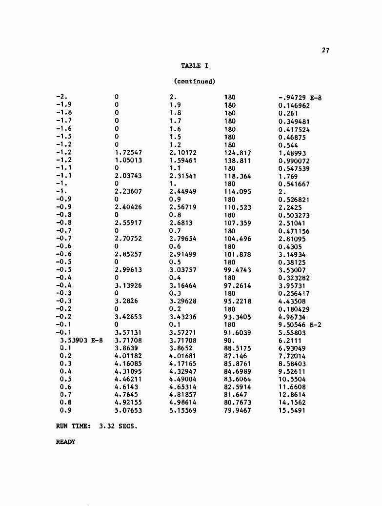