
Application of Machine Learning to Financial Time Series ...
220
1 Application of Machine Learning to Financial Time Series Analysis Martin Victor Sewell Thesis submitted for the degree of Doctor of Philosophy of UCL Department of Computer Science University College London University of London 2017
Transcript of Application of Machine Learning to Financial Time Series ...

1
Application of Machine Learning to FinancialTime Series Analysis
Martin Victor Sewell
Thesis submitted for the degree of
Doctor of Philosophy
of
UCL
Department of Computer Science
University College London
University of London
2017

2
I, Martin Victor Sewell, confirm that the work presented in this thesis is my own. Where information
has been derived from other sources, I confirm that this has been indicated in the thesis.

Abstract 3
Abstract
This multidisciplinary thesis investigates the application of machine learning to financial time series
analysis. The research is motivated by the following thesis question: ‘Can one improve upon the state of
the art in financial time series analysis through the application of machine learning?’ The work is split
according to the following time series trichotomy: 1) characterization — determine the fundamental
properties of the time series; 2) modelling — find a description that accurately captures features of the
long-term behaviour of the system; and 3) forecasting — accurately predict the short-term evolution of
the system.
Characterization
The research on characterization to determine fundamental properties comprises five experiments. They
all relate to implementing algorithms that test the cornerstone of modern financial theory, the efficient
market hypothesis. In tests for dependence, tests for autocorrelation and two runs tests are applied to
US stock market returns and six foreign exchange currency pairs. Results showed that daily DJIA,
USD/DEM, USD/JPY, GBP/USD, USD/CHF and GBP/CHF returns each exhibit a surprising number
of sequences of decreasing returns. In a test for long memory, my implementation of Hurst’s rescaled
range (R/S) analysis (in C++) found little evidence of long memory in US stock market returns. In a
test of market efficiency, the performance of investment newsletters is analysed, evidencing weak-form
efficiency. All five experiments (potentially) have implications apropos market efficiency, and impart
domain knowledge vis-a-vis financial time series for the work on forecasting.
Modelling
The work on modelling to capture long-term behaviour utilizes behavioural finance to 1) model market
action and 2) model investors’ risk preferences. For the former, in order to model as accurately as
possible, minimal assumptions are made and a bottom-up approach is used. The evolved heuristics
and biases exhibited by fundamental analysts and technical analysts are used to build an agent-based
artificial stock market (in Excel). The proportion of technical analysts is varied and the statistics of the
time series generated by the artificial market analysed. In the second part, in order to accurately model
decision making under uncertainty in practice I adopt the seminal psychological (descriptive), rather

4 Abstract
than economic (normative), formulation, prospect theory. I devise and implement (in PHP and VB) an
investment performance measurement metric, cumulative prospect theory certainty equivalent (CPTCE).
Forecasting
The research on forecasting concerns the prediction of financial markets. First domain knowledge gained
via the runs test is used to build a DJIA trading system. I then use kernel methods, a recent, successful and
computationally efficient class of algorithms used for pattern analysis. A hidden Markov model (HMM)
is trained on foreign exchange data to derive a Fisher kernel (which I implement in C++) for a support
vector machine (SVM), and the (difference of convex functions) DC algorithm and the Bayes point
machine are also used to create kernels. Furthermore, the DC algorithm is used to learn the parameters
of the HMM in the Fisher kernel. I ported two implementations of SVMs to Windows and also added
semi-automated parameter selection. SVMdark is written in C for Win32, and winSVM in C++ for
Win32.
Contributions to Science
The thesis is believed to make several novel contributions to science, it is multidisciplinary with con-
tributions to both computer science and finance. In the work on characterization I wrote software for
performing the runs test and testing for long-memory. I then reconcile the fact that daily stock mar-
ket and foreign exchange log returns pass linear statistical tests of efficiency, yet non-linear forecasting
methods can still make above-average risk-adjusted returns, and the nature of the inefficiencies are iden-
tified. In the research on modelling the agent-based artificial stock market generated a time series that
provides a novel insight into the effect of the proportion of technical analysts relative to fundamental
analysts. Whilst the novel investment performance measurement metric, cumulative prospect theory
certainty equivalent (CPTCE), models investors’ empirically-observed risk preferences, whilst no other
performance metric does this effectively. The experiments on forecasting included using the DC algo-
rithm to learn the parameters of the hidden Markov model in the Fisher kernel, this is a novel algorithm.
Two Windows implementations of SVMs with semi-automated parameter selection were built, for some
time they were the only Windows applications dedicated to support vector machines.

Acknowledgements 5
Acknowledgements
Firstly, I wish to thank my supervisor Philip Treleaven for providing me with the opportunity to embark
upon a PhD in the first place. Thanks also to David Corney for acting as a mentor. Thanks to John
Campbell for sparking my interest in multiagent systems. For general help within the department I thank
Chris Clack, and for friendship and collaboration Wei Yan. Thanks to Hurst Consulting and INLECOM
for sponsorship. Thanks to Salus Alpha, Fortress Investment Group, Anova Fund, Global Advisors and
eStats Capital for providing data. Thanks to Brian McIntosh and Paul Jeffrey of The School of Water
Sciences at Cranfield University for employment, and thanks to Christopher Lucas for work with Cirrus
Capital.
Thanks to my UCL drinking companions Robert, David, Emma B., Miles, Michael, Dirk, Gordon,
Bill, Tim and Emma T for many great evenings, and thanks to Robert and Nancy for helping me stop.
Thanks to Julie D., Philippa, Emma, Michael, Nancy, John & Zoe, Vanessa, Petya, Christophe, Valerie,
Sauminh, Bill, Carol, Amy, Monica, Wei, Niklas, Lai Nee, Tristan, Tom, Jon, Vicki, Julie Z., Qi, Flo-
rence, Julie K., Kiri, Jas, Maya, Lucia and my parents for feeding me at various times. Many thanks to
Nancy for always being there. Thanks to Carol for accompanying me on several trips to the cinema in
Bedford. Thanks to Vicki for many pleasant days out. Eternal thanks to Zac Harland for sharing his un-
bridled enthusiasm and extensive knowledge of trading over numerous and regular coffees in the Gower
Street bookshop. Thanks to my clubbing friends Dave, Amanda, Jim, Rose, Rosie, et al. for festivals,
fun and keeping me young.
Thank you to Robert Dodier for convincing me of the superiority of probability right from the start.
Thanks to David Wolpert for quick and helpful replies to my queries on the no free lunch theorems, to
Andrew Lo for clarifying the EMH and to Eugene Fama for a historical correction. Thanks to our ex-
Head of Department, Anthony Finkelstein, for having faith in me. For comments on drafts of this thesis,
I thank David Corney, Monica Diekmann-Kotzee, Anthony Finkelstein, John Shawe-Taylor, Christophe
Cuny, Niklas Traub, Bill Langdon, Zac Harland, Miles Hansard, Robin Hankin, Professor Treleaven and
my parents. A special thanks are due to Professor Shawe-Taylor for algorithmic suggestions and thanks
to Professor Treleaven for guidance on the home straight and helping me turn a book into a thesis. Thanks
also to David Barber, Edward Tsang, Christoph Schommer, Ricardo Silva and anonymous reviewers for
various corrections and suggestions. With a view to future work, thanks to Adam Johansen for help
regarding particle filters and thanks for communications with Frank Lad, surely the purest subjectivist
Bayesian since de Finetti. Thanks to Wei Si for spotting an error.

6 Acknowledgements
I would also like to thank Chris Neely for numerous emails patiently detailing the methodology
used in his work with Paul Weller. In Cambridge, thanks to the directors of 4CMR Terry Barker and
Doug Crawford-Brown for their generous and patient support, thanks to Robin Hankin for his rigorous
approach to science. Thanks also to Mairead, Annela, Svetlana, Paul, Mark, Jun Li, Yongfu and the
rest of 4CMR for putting up with me. Thanks to Stephen Stretton, a work colleague and friend, for his
intelligent insight. Thanks also to Richard Schuhmertl from Quant Capital for recognising my potential
and providing me with a great opportunity. A special mention to Julie Kim, whose texts and company
make me smile. Thanks to Jas for her eternal cheekiness. Thanks to Anouska and Freddie for being there.
Naturally, eternal thanks go to my parents for their life-long support. Thanks to luck for my ability to
select the unique model Talisa Qi, the only model that was right. Finally, thank god I’ve finished.

Contents 7
Contents
Abstract 3
Publications 15
1 Introduction 17
1.1 Motivations . . . . . . . . . . . . . . . . . . . . . . . . . . . . . . . . . . . . . . . . . 17
1.2 Research Objectives . . . . . . . . . . . . . . . . . . . . . . . . . . . . . . . . . . . . . 19
1.3 Research Methodology . . . . . . . . . . . . . . . . . . . . . . . . . . . . . . . . . . . 19
1.3.1 Characterization . . . . . . . . . . . . . . . . . . . . . . . . . . . . . . . . . . 19
1.3.2 Modelling . . . . . . . . . . . . . . . . . . . . . . . . . . . . . . . . . . . . . . 20
1.3.3 Forecasting . . . . . . . . . . . . . . . . . . . . . . . . . . . . . . . . . . . . . 21
1.4 Contributions to Science . . . . . . . . . . . . . . . . . . . . . . . . . . . . . . . . . . 22
1.5 Chapters . . . . . . . . . . . . . . . . . . . . . . . . . . . . . . . . . . . . . . . . . . . 24
2 Background and Literature Review 27
2.1 Introduction . . . . . . . . . . . . . . . . . . . . . . . . . . . . . . . . . . . . . . . . . 27
2.2 Efficient Market Hypothesis . . . . . . . . . . . . . . . . . . . . . . . . . . . . . . . . 28
2.3 Characterization . . . . . . . . . . . . . . . . . . . . . . . . . . . . . . . . . . . . . . . 29
2.3.1 Markets . . . . . . . . . . . . . . . . . . . . . . . . . . . . . . . . . . . . . . . 30
2.3.2 Time Series . . . . . . . . . . . . . . . . . . . . . . . . . . . . . . . . . . . . . 30
2.3.3 Stochastic Processes in Financial Markets . . . . . . . . . . . . . . . . . . . . . 30
2.3.4 Stylized Facts . . . . . . . . . . . . . . . . . . . . . . . . . . . . . . . . . . . . 32
2.3.5 Dependence in Market Returns . . . . . . . . . . . . . . . . . . . . . . . . . . . 32
2.3.6 Long Memory in Market Returns . . . . . . . . . . . . . . . . . . . . . . . . . 34
2.3.7 Investment Newsletters . . . . . . . . . . . . . . . . . . . . . . . . . . . . . . . 37
2.4 Modelling . . . . . . . . . . . . . . . . . . . . . . . . . . . . . . . . . . . . . . . . . . 39
2.4.1 Behavioural Finance . . . . . . . . . . . . . . . . . . . . . . . . . . . . . . . . 39
2.4.2 Technical Analysis . . . . . . . . . . . . . . . . . . . . . . . . . . . . . . . . . 41
2.4.3 Multiagent Systems . . . . . . . . . . . . . . . . . . . . . . . . . . . . . . . . . 44
2.4.4 Prospect Theory . . . . . . . . . . . . . . . . . . . . . . . . . . . . . . . . . . 44
2.4.5 Investment Performance Measurement . . . . . . . . . . . . . . . . . . . . . . . 46

8 Contents
2.5 Forecasting . . . . . . . . . . . . . . . . . . . . . . . . . . . . . . . . . . . . . . . . . 47
2.5.1 No Free Lunch Theorem for Supervised Machine Learning . . . . . . . . . . . . 47
2.5.2 Data Snooping . . . . . . . . . . . . . . . . . . . . . . . . . . . . . . . . . . . 48
2.5.3 Kernel Methods . . . . . . . . . . . . . . . . . . . . . . . . . . . . . . . . . . . 48
2.5.4 Support Vector Machines . . . . . . . . . . . . . . . . . . . . . . . . . . . . . . 49
2.5.5 Genetic Programming . . . . . . . . . . . . . . . . . . . . . . . . . . . . . . . 52
3 Characterization 55
3.1 Data . . . . . . . . . . . . . . . . . . . . . . . . . . . . . . . . . . . . . . . . . . . . . 55
3.2 Autocorrelation . . . . . . . . . . . . . . . . . . . . . . . . . . . . . . . . . . . . . . . 56
3.3 Runs Test . . . . . . . . . . . . . . . . . . . . . . . . . . . . . . . . . . . . . . . . . . 57
3.3.1 First Runs Test . . . . . . . . . . . . . . . . . . . . . . . . . . . . . . . . . . . 58
3.3.2 Second Runs Test . . . . . . . . . . . . . . . . . . . . . . . . . . . . . . . . . . 58
3.4 Long Memory . . . . . . . . . . . . . . . . . . . . . . . . . . . . . . . . . . . . . . . . 60
3.5 Investment Newsletters . . . . . . . . . . . . . . . . . . . . . . . . . . . . . . . . . . . 61
3.6 Conclusion and Summary . . . . . . . . . . . . . . . . . . . . . . . . . . . . . . . . . . 63
4 Modelling 65
4.1 An Artificial Stock Market . . . . . . . . . . . . . . . . . . . . . . . . . . . . . . . . . 65
4.1.1 Design . . . . . . . . . . . . . . . . . . . . . . . . . . . . . . . . . . . . . . . 65
4.1.2 Implementation . . . . . . . . . . . . . . . . . . . . . . . . . . . . . . . . . . . 66
4.1.3 Testing . . . . . . . . . . . . . . . . . . . . . . . . . . . . . . . . . . . . . . . 72
4.2 Investment Performance Measurement . . . . . . . . . . . . . . . . . . . . . . . . . . . 76
4.2.1 Design . . . . . . . . . . . . . . . . . . . . . . . . . . . . . . . . . . . . . . . 76
4.2.2 Implementation . . . . . . . . . . . . . . . . . . . . . . . . . . . . . . . . . . . 78
4.2.3 Testing . . . . . . . . . . . . . . . . . . . . . . . . . . . . . . . . . . . . . . . 80
4.3 Conclusion and Summary . . . . . . . . . . . . . . . . . . . . . . . . . . . . . . . . . . 81
5 Forecasting 83
5.1 Forecasting DJIA Daily Returns . . . . . . . . . . . . . . . . . . . . . . . . . . . . . . 83
5.2 Kernel Methods . . . . . . . . . . . . . . . . . . . . . . . . . . . . . . . . . . . . . . . 84
5.3 Design . . . . . . . . . . . . . . . . . . . . . . . . . . . . . . . . . . . . . . . . . . . . 85
5.4 Implementation . . . . . . . . . . . . . . . . . . . . . . . . . . . . . . . . . . . . . . . 99
5.5 Testing . . . . . . . . . . . . . . . . . . . . . . . . . . . . . . . . . . . . . . . . . . . . 104
5.6 Conclusion and Summary . . . . . . . . . . . . . . . . . . . . . . . . . . . . . . . . . . 108
6 Assessment 109
6.1 Hypothesis . . . . . . . . . . . . . . . . . . . . . . . . . . . . . . . . . . . . . . . . . 109
6.2 Precision . . . . . . . . . . . . . . . . . . . . . . . . . . . . . . . . . . . . . . . . . . 110
6.3 Thoroughness . . . . . . . . . . . . . . . . . . . . . . . . . . . . . . . . . . . . . . . . 111

Contents 9
6.4 Contributions . . . . . . . . . . . . . . . . . . . . . . . . . . . . . . . . . . . . . . . . 116
6.5 Comparison with Similar Work of Others . . . . . . . . . . . . . . . . . . . . . . . . . 118
6.6 Conclusion and Summary . . . . . . . . . . . . . . . . . . . . . . . . . . . . . . . . . . 122
7 Conclusion and Future Work 123
7.1 Conclusion . . . . . . . . . . . . . . . . . . . . . . . . . . . . . . . . . . . . . . . . . 123
7.2 Further Work . . . . . . . . . . . . . . . . . . . . . . . . . . . . . . . . . . . . . . . . 126
A ISO 4217 Currency Codes 135
B Exchanges and Stock Market Indices 137
B.1 Exchanges . . . . . . . . . . . . . . . . . . . . . . . . . . . . . . . . . . . . . . . . . . 137
B.2 Stock Market Indices . . . . . . . . . . . . . . . . . . . . . . . . . . . . . . . . . . . . 139
C Time Series Glossary 141
D Runs Tests Source Code 143
E Runs Tests on DJIA Returns 153
F Runs Tests on Foreign Exchange Returns 159
G Rescaled Range Analysis Source Code 167
H Technical Analysis Taxonomy 171
I Cumulative Prospect Theory Certainty Equivalent Source Code 173
J Kernel Methods/Support Vector Machines 183
J.1 Gram Matrix . . . . . . . . . . . . . . . . . . . . . . . . . . . . . . . . . . . . . . . . 183
J.2 Hilbert Space . . . . . . . . . . . . . . . . . . . . . . . . . . . . . . . . . . . . . . . . 183
K Fisher Kernel Source Code 185
L Similar Publications 189
Bibliography 191

10 Contents

List of Figures 11
List of Figures
2.1 A hypothetical value function in prospect theory . . . . . . . . . . . . . . . . . . . . . . 45
2.2 Weighting functions for gains and losses in cumulative prospect theory . . . . . . . . . . 46
4.1 Mean log return (P&L) per analyst . . . . . . . . . . . . . . . . . . . . . . . . . . . . . 73
4.2 Mean Sharpe ratio per analyst . . . . . . . . . . . . . . . . . . . . . . . . . . . . . . . 74
4.3 Statistics of price log returns . . . . . . . . . . . . . . . . . . . . . . . . . . . . . . . . 74
4.4 Kurtosis of price log returns . . . . . . . . . . . . . . . . . . . . . . . . . . . . . . . . 75
4.5 Autocorrelations of price log returns . . . . . . . . . . . . . . . . . . . . . . . . . . . . 75
4.6 Maximal Sharpe ratio . . . . . . . . . . . . . . . . . . . . . . . . . . . . . . . . . . . . 78
5.1 Forecasting DJIA daily returns equity curve . . . . . . . . . . . . . . . . . . . . . . . . 84
5.2 SVMdark . . . . . . . . . . . . . . . . . . . . . . . . . . . . . . . . . . . . . . . . . . . 88
5.3 winSVM . . . . . . . . . . . . . . . . . . . . . . . . . . . . . . . . . . . . . . . . . . . 89
5.4 Rolling window data sets . . . . . . . . . . . . . . . . . . . . . . . . . . . . . . . . . . 101
6.1 Net market exposure for various strategies in equities . . . . . . . . . . . . . . . . . . . 115

12 List of Figures

List of Tables 13
List of Tables
2.1 Stochastic processes and their applicability to markets . . . . . . . . . . . . . . . . . . . 31
3.1 Autocorrelation of DJIA log returns . . . . . . . . . . . . . . . . . . . . . . . . . . . . 57
3.2 Autocorrelation of foreign exchange log returns . . . . . . . . . . . . . . . . . . . . . . 57
3.3 Runs of DJIA log returns above and below the mean . . . . . . . . . . . . . . . . . . . 58
3.4 Runs of foreign exchange log returns above and below the mean . . . . . . . . . . . . . 59
3.5 Rescaled range analysis on detrended DJIA log returns . . . . . . . . . . . . . . . . . . 62
3.6 ‘Up markets’ and ‘down markets’ as defined by the ‘Forbes/Hulbert investment letter
survey’ . . . . . . . . . . . . . . . . . . . . . . . . . . . . . . . . . . . . . . . . . . . 62
3.7 Correlation matrix of ‘The Forbes/Hulbert investment letter survey’ . . . . . . . . . . . 63
3.8 The extent to which the four statistical tests rejected weak form market efficiency across
different time periods. . . . . . . . . . . . . . . . . . . . . . . . . . . . . . . . . . . . . 64
4.1 Statistics of daily stock log returns . . . . . . . . . . . . . . . . . . . . . . . . . . . . . 72
4.2 Statistics generated by the artificial stock market . . . . . . . . . . . . . . . . . . . . . . 73
4.3 Range of proportions of technical analysts in the artificial stock market that replicate
stylized facts . . . . . . . . . . . . . . . . . . . . . . . . . . . . . . . . . . . . . . . . 76
4.4 Sharpe ratio and CPTCE correlations . . . . . . . . . . . . . . . . . . . . . . . . . . . . 81
5.1 Pseudocode for the fixed length HMM kernel . . . . . . . . . . . . . . . . . . . . . . . 92
5.2 Fisher kernel test results . . . . . . . . . . . . . . . . . . . . . . . . . . . . . . . . . . 99
5.3 Fisher kernel symbol allocation . . . . . . . . . . . . . . . . . . . . . . . . . . . . . . . 102
5.4 Out of sample results, USD/DEM . . . . . . . . . . . . . . . . . . . . . . . . . . . . . 104
5.5 Out of sample results, USD/JPY . . . . . . . . . . . . . . . . . . . . . . . . . . . . . . 105
5.6 Out of sample results, GBP/USD . . . . . . . . . . . . . . . . . . . . . . . . . . . . . . 105
5.7 Out of sample results, USD/CHF . . . . . . . . . . . . . . . . . . . . . . . . . . . . . . 105
5.8 Out of sample results, DEM/JPY . . . . . . . . . . . . . . . . . . . . . . . . . . . . . . 106
5.9 Out of sample results, GBP/CHF . . . . . . . . . . . . . . . . . . . . . . . . . . . . . . 106
5.10 Out of sample results, Mean . . . . . . . . . . . . . . . . . . . . . . . . . . . . . . . . 106
5.11 Summary of results on forecasting . . . . . . . . . . . . . . . . . . . . . . . . . . . . . 108
E.1 DJIA daily returns: increasing . . . . . . . . . . . . . . . . . . . . . . . . . . . . . . . 153

14 List of Tables
E.2 DJIA daily returns: decreasing . . . . . . . . . . . . . . . . . . . . . . . . . . . . . . . 154
E.3 DJIA weekly returns: increasing . . . . . . . . . . . . . . . . . . . . . . . . . . . . . . 154
E.4 DJIA weekly returns: decreasing . . . . . . . . . . . . . . . . . . . . . . . . . . . . . . 155
E.5 DJIA monthly returns: increasing . . . . . . . . . . . . . . . . . . . . . . . . . . . . . 155
E.6 DJIA monthly returns: decreasing . . . . . . . . . . . . . . . . . . . . . . . . . . . . . 156
E.7 DJIA annual returns: increasing . . . . . . . . . . . . . . . . . . . . . . . . . . . . . . 156
E.8 DJIA annual returns: decreasing . . . . . . . . . . . . . . . . . . . . . . . . . . . . . . 157
F.1 USD/DEM daily returns: increasing . . . . . . . . . . . . . . . . . . . . . . . . . . . . 159
F.2 USD/DEM daily returns: decreasing . . . . . . . . . . . . . . . . . . . . . . . . . . . . 160
F.3 USD/JPY daily returns: increasing . . . . . . . . . . . . . . . . . . . . . . . . . . . . . 160
F.4 USD/JPY daily returns: decreasing . . . . . . . . . . . . . . . . . . . . . . . . . . . . . 161
F.5 GBP/USD daily returns: increasing . . . . . . . . . . . . . . . . . . . . . . . . . . . . . 161
F.6 GBP/USD daily returns: decreasing . . . . . . . . . . . . . . . . . . . . . . . . . . . . 162
F.7 USD/CHF daily returns: increasing . . . . . . . . . . . . . . . . . . . . . . . . . . . . . 162
F.8 USD/CHF daily returns: decreasing . . . . . . . . . . . . . . . . . . . . . . . . . . . . 163
F.9 DEM/JPY daily returns: increasing . . . . . . . . . . . . . . . . . . . . . . . . . . . . . 163
F.10 DEM/JPY daily returns: decreasing . . . . . . . . . . . . . . . . . . . . . . . . . . . . 164
F.11 GBP/CHF daily returns: increasing . . . . . . . . . . . . . . . . . . . . . . . . . . . . . 164
F.12 GBP/CHF daily returns: decreasing . . . . . . . . . . . . . . . . . . . . . . . . . . . . 165

PUBLICATIONS 15
Publications
The research in this thesis has resulted in 25 publications in total (12 peer reviewed): 5 journal articles,
5 conference proceedings, 1 book chapter and 6 technical reports, as listed below. The key publications
are shown in bold.
Patel, N. and Sewell, M. (2015), Calendar anomalies: A survey of the literature, International Journal
of Behavioural Accounting and Finance 5(2), 99–121.
Sewell, M. (2012a), The efficient market hypothesis: Empirical evidence, International Journal of
Statistics and Probability 1(2), 164–178.
Sewell, M. (2012b), The demarcation of science, Young Statisticians’ Meeting, Cambridge, 2–3 April
2012.
Sewell, M. (2012c), An artificial stock market, in J. Filipe and A. Fred (eds.), ICAART 2012: Pro-
ceedings of the 4th International Conference on Agents and Artificial Intelligence, Volume 2. Vil-
amoura, Algarve, Portugal, 6 - 8 February, 2012, SciTePress, Setubal, pp.293–300.
Sewell, M. (2012d), Ideology-free politics: A bottom-up approach, CRASSH Postdoctoral Research
Seminar Series. Cambridge, 21 June 2012.
Sewell, M. (2012e), The philosophy of risk, in URMPM World Congress 2012 in London. “The Human
Factor in Risk”. Proceedings, Union of Risk Management for Preventive Medicine (URMPM), p.80.
Sewell, M. and Shawe-Taylor, J. (2012), Forecasting foreign exchange rates using kernel methods,
Expert Systems with Applications 39(9), 7652–7662.
Sewell, M. (2011a), The evolution of entrepreneurs and venture capitalists, in R. Yazdipour (ed.), Ad-
vances in Entrepreneurial Finance: With Applications from Behavioral Finance and Economics,
Springer, New York, Chapter 11, pp.205–217.
Sewell, M. (2011b), Characterization of financial time series, Research Note RN/11/01, University Col-
lege London, London.
Sewell, M. (2011c), Ensemble learning, Research Note RN/11/02, University College London, London.
Sewell, M. (2011d), Fund performance, Research Note RN/11/03, University College London, London.

16 PUBLICATIONS
Sewell, M. (2011e), History of the efficient market hypothesis, Research Note RN/11/04, University
College London, London.
Sewell, M. (2011f), Money management, Research Note RN/11/05, University College London, London.
Sewell, M. (2011g), The Fisher kernel: A brief review, Research Note RN/11/06, University College
London, London.
Sewell, M. (2011h), Psychology of successful investing, behaviouralfinance.net, 12 February 2011.
Sewell, M. (2011i), Human behaviour under risk and uncertainty: Are we really just conservative?,
envecon 2011: Applied Environmental Economics Conference, London, 4 March 2011.
Sewell, M. (2010a), Introduction to behavioural finance, behaviouralfinance.net, 14 April 2010.
Sewell, M. (2010b), Emotions help solve the prisoner’s dilemma, Behavioural Finance Working Group
Conference: Fairness, Trust and Emotions in Finance, London, 1–2 July 2010.
Sewell, M., Schuhmertl, R., Wei, J. and Harris, D. (2010), Quant Capital’s M&A Strategy, 19 June 2010.
Sewell, M. (2009a), Algorithm bias: A statistical review, Futures pp.38–40.
Sewell, M. (2009b), Decision making under risk: A prescriptive approach, in Proceedings of the 2009
Symposium; Academy of Behavioral Finance and Economics, September 23-25, 2009, Chicago, Illi-
nois, Academy of Behavioral Finance and Economics, Montrose, CA, p.9.
Sewell, M. (2008a), Optimization and methods to avoid overfitting, Talk presented at the Automated
Trading 2008 conference, London, 15 October 2008.
Sewell, M. (2008b), Gender (sic) equality (sic), Opticon1826 4.
Sewell, M. V. and Yan, W. (2008), Ultra high frequency financial data, in M. Keijzer (ed.), Proceedings
of the 2008 GECCO Conference Companion on Genetic and Evolutionary Computation, ACM, New
York, pp.1847–1850.
Yan, W., Sewell, M. V. and Clack, C. D. (2008), Learning to optimize profits beats predicting returns —
comparing techniques for financial portfolio optimisation, in M. Keijzer (ed.), Proceedings of the 10th
Annual Conference on Genetic and Evolutionary Computation, ACM, New York, pp.1681–1688.

17
Chapter 1
Introduction
This chapter sets the scene. It starts with my motivations for undertaking the work, and
explains why the area of research is important. It continues with the research objectives
including the research question, the research methodology for the chapters on character-
ization, modelling and forecasting and then lists the all important contributions made to
science. The chapter finishes with an annotated guide to each chapter in the thesis.
1.1 Motivations
This thesis concerns the application of machine learning to the understanding of financial markets. A
greater understanding of financial markets is important, if only because of their impact on the global
economy. Back in 1929 the Wall Street Crash caused the Dow Jones Industrial Average (DJIA) to lose
40 per cent of its value in two months. In 1992 in the UK, the events that took place on Black Wednesday
when sterling was forced out of the ERM are an example of when the markets were more powerful than
the governments; the markets were right in the sense that the devaluation forced on sterling was justified
by the country’s economic dilemma. A third example concerns the ‘dot-com bubble’, the DJIA tripled
between 1994 and 1999, whilst, over the same period, basic economic indicators did not come close
to tripling. The global financial crisis of 2007–08 led to a downturn in the housing market, evictions,
foreclosures, the failure of businesses, unemployment, huge declines in consumer wealth and a downturn
in economic activity. Lastly, daily foreign exchange market turnover averaged $5.3 trillion in April 2013
(Bank for International Settlements, 2013). This is over 17 times greater than the gross domestic product
(GDP) of the world economy and over 100 times greater than global exports.
Gershenfeld and Weigend (1994) claim that [t]ime series analysis has three goals: forecasting,
modeling, and characterization. I utilize their time series trichotomy, albeit in a different order, and
applied it to financial time series to structure the core of the thesis thus.
The research on characterization in this thesis is partially motivated because it imparts domain
knowledge for the work on forecasting. It is also motivated by the challenge itself, for example the
distribution of financial market returns is not precisely known.

18 Chapter 1. Introduction
The markets uniquely capture the psychology of individuals on a large scale. Markets usually reflect
the decisions of thousands or even millions of people going about their daily lives. The sheer size of the
markets also makes the area research-worthy and non-trivial. Multiagent systems would appear the most
natural way of modelling a market when the market participants are both numerous and autonomous.
The task of forecasting financial markets is one of predicting a time series generated from a social
science, which in practice is purely an exercise in information processing. An attractive way of achiev-
ing this is to make minimal assumptions and use a data-driven, model-free, flexible and nonparametric
approach. In other words, use machine learning, in the guise of supervised learning, which encompasses
both theoretical soundness and experimental effectiveness. The central paradigm in the model-driven
domain of finance is the ‘efficient market hypothesis’ (EMH), and an efficient market is one in which
prices always ‘fully reflect’ available information. This creates a challenge, as it implies that ‘beating
the market’ by forecasting changes in price is at best very difficult, and at worst impossible. The EMH
is thus important because it places restrictions on what is possible vis-a-vis forcasting algorithms. The
research on forecasting is thus partially motivated because it creates the potential to challenge the central
paradigm in finance, the EMH. Plus it presents the potential to improve supervised learning algorithms.
Another motivation for focussing on finance is that the research domain is growing. As technology
drives down transaction costs, markets are increasingly accessible to an increasing number of partic-
ipants. Also, globally, the failure of communism has ensured that the market economy continues to
grow.
In addition to the research described in this thesis, there exists an array of opportunities for further
work in this field. Algorithmic trading typically involves splitting up an order to buy or sell a fixed
number of shares in an optimal manner over a period of time; this is extremely fertile territory for the
application of machine learning. Intelligent techniques could be used to optimize a trading system based
on cointegration. Deep learning algorithms could be used to forecast financial time series, as they should
be able to find and exploit signals at different levels of abstraction. Ensemble learning could be used
to attempt to combine individual predictive models in an optimal way. An equity trading system could
be built using the knowledge gained from the characterization of equity markets. Intelligent techniques
could be employed to select funds and allocate capital. Quantitative techniques could be applied to
global macro hedge fund strategies. Optimizing an automated market-making algorithm using intelligent
techniques could be hugely lucrative for the financial industry. In the area of mergers and acquisitions,
machine learning could be applied to the potentially lucrative task of predicting takeover targets. Once a
trader has found a positive expected return, they need to decide what proportion of their capital to bet per
trade: money management and position sizing are a challenging optimization problem. Another potential
source of enormous wealth would be the application of intelligent techniques to option pricing. Rather
than just the price, or the bid and the ask, an intelligent trading system could utilize several levels of the
order book. A probabilistic model such as a particle filter could be employed to track a financial time
series. Finally, intelligent techniques could be employed to predict yield curves. Section 7.2 (p. 126)
addresses potential ideas for further work and goes into more detail.

1.2. Research Objectives 19
My interests in developing the work further mainly concern working with ultra high frequency
financial data. Tick data, preferably showing the order book, must be ripe for exploitation by machine
learning, but would require impressive processing power, a vast amount of storage and robust algorithms.
Today, tick data generated by financial markets quite possibly represents a greater volume than any other
source outside high energy physics. Futures markets provide the most data, followed by foreign exchange
markets, followed by stock markets, although most of the literature relates to stock markets. It is likely
that the type of modelling required would be similar across all three types of market. In practice, we are
more likely to be concerned with futures markets or foreign exchange markets because transaction costs
are vanishingly small and leverage is possible.
1.2 Research Objectives
The thesis research question is: ‘Can one improve upon the state of the art in financial time series analysis
through the application of machine learning?’ The thesis is split according to the three above-identified
central areas of time series analysis: characterization, modelling and forecasting.
characterization Characterization attempts with little or no a priori knowledge to determine fundamen-
tal properties, such as the stationarity of a system or the amount of randomness.
modelling The goal of modelling is to find a description that accurately captures features of the long-
term behaviour of the system.
forecasting The aim of forecasting (also called predicting) is to accurately predict the short-term evolu-
tion of the system.
In the forecasting third of the thesis the aims may be graduated thus: 1) to improve standard algorithms,
and 2) to beat the ‘state of the art’. The more ambitious goal, 2), is ill-defined, as there is no consensus
within academia and it is likely to be proprietary outside, but an algorithm that successfully forecast
financial markets published in the academic literature shall be used as a proxy.
1.3 Research Methodology
1.3.1 Characterization
The goals of the research on characterization (Chapter 3) are to write efficient implementations of al-
gorithms that contribute to the ‘stylized facts’1 of financial markets. Five experiments are conducted.
The experiments are chosen because they are tests of market efficiency, and help us to characterize fi-
nancial markets. A test of autocorrelation and two versions of the runs test (a non-parametric test of
the mutual dependence of the elements of a sequence) were performed on the DJIA and six foreign ex-
change currency pairs. Results showed that daily DJIA, USD/DEM, USD/JPY, GBP/USD, USD/CHF1A stylized fact is a term used in economics to refer to empirical findings that are so consistent (for example, across a wide
range of instruments, markets and time periods) that they are accepted as truth. Due to their generality, they are often qualitative.

20 Chapter 1. Introduction
and GBP/CHF returns each exhibit a surprising number of sequences of decreasing returns. Whilst my
implementation of Hurst’s rescaled range (R/S) analysis (in C++) found little evidence of long memory
in stock market returns. My implementation of R/S analysis is more accurate than commercially avail-
able software, but slower. I purchased ‘The Forbes/Hulbert investment letter survey’, the data encom-
passes performance from 31 May 1990 to 31 December 2001 and includes just those newsletters tracked
that have a predominant US equity focus. The performance of the recommendations of the newsletters is
analysed by means of correlation analysis on the quantitative data and the results evidenced weak-form
market efficiency.
1.3.2 Modelling
The goals of the experiments on modelling are to improve algorithms that 1) model market action (Sec-
tion 4.1) and 2) model investors’ risk preferences (Section 4.2). The experiments are chosen because they
each allow us to model markets and investors’ risk preferences using a realistic bottom-up empiricallly-
valid approach, with a focus on simplicity and realism. Both experiments utilize behavioural finance. For
the former, the evolved heuristics and biases exhibited by fundamental analysts and technical analysts,
such as representativeness and conservatism, are used to build an agent-based artificial stock market
(in Excel). The relative proportion of technical analysts and fundamental analysts was allowed to vary,
leading to the following broad conclusions. Whether a fundamental analyst, or a technical analyst, it
pays to be in a majority. As the number of technical analysts increases, the standard deviation of returns
decreases, whilst the skewness increases. Whilst kurtosis of market returns peaks with around 40 per
cent technical analysts, and rapidly declines as the number of technical analysts exceeds 90 per cent.
The autocorrelation of returns is close to zero with 100 per cent fundamental analysts, and approaches
1.0 as the proportion of technical analysts approaches 100 per cent. With a realistic proportion of tech-
nical analysts and fundamental analysts, the artificial stock market replicates mean returns, the standard
deviation of returns, the absolute returns correlation and the squared returns correlation of a real stock
market. However, the artificial stock market failed to accurately replicate the skewness, kurtosis and au-
tocorrelation of returns. The number of free parameters was kept to a minimum, so there was little scope
for tuning the model until it output the desired results. In the second part, I devised and implemented (in
both PHP and Visual Basic) an investment performance measurement metric developed from prospect
theory (Kahneman and Tversky, 1979; Tversky and Kahneman, 1992) known as cumulative prospect
theory certainty equivalent (CPTCE). The implementation of CPTCE makes up part of a more general
performance measurement calculator which I wrote and is freely available online.2 It calculates mean
return, standard deviation, skewness, kurtosis, beta, Jensen’s alpha, Sharpe ratio, Sortino ratio, Treynor’s
measure, information ratio, Stutzer ratio, Omega, M2, T2 and maximum drawdown, and is in use by the
financial industry.
2http://www.performance-measurement.org

1.3. Research Methodology 21
1.3.3 Forecasting
The goals of the experiments on forecasting are to 1) improve standard algorithms, and 2) beat the ‘state
of the art’. We have shown that forecasting financial markets is at best very difficult. Furthermore, if
a simple algorithm were able to generate abnormal returns, the algorithm would be adopted by many
market participants, and the pattern in the time series that the algorithm was exploiting would become
eroded as traders attempted to enter the market ahead of each other, so the algorithm would cease being
profitable. On the other hand, it seems unlikley that there exists a highly complex pattern in financial
time series that is exploitable, because it would likley be swamped by noise. We are left with the task of
seeking unknown patterns of intermediate complexity.
First domain knowledge gained via the runs test is used to build a DJIA trading system (Section 5.1).
Although the algorithm is created ‘in sample’, given its simplicity and the size of the data set, significant
overfitting of noise seems unlikely, so the equity curve is surprisingly impressive up until 2002, when
the dynamics of the market must have changed. However, the algorithm clearly fails to outperform the
market in the out of sample period.
For both theoretical and empirical reasons I then opt to use kernel methods for forecasting (Sec-
tion 5.2). Detecting linear relations has been the focus of much research in statistics and machine learn-
ing for decades and the resulting algorithms are well understood, well developed and efficient. However,
linearity is rather special, and outside quantum mechanics no real system is truly linear (Meiss, 2003).
Naturally, one wants the best of both worlds. So, if a problem is non-linear, instead of trying to fit a
non-linear model, one can map the problem from the input space to a new (higher-dimensional) space
(called the feature space) by doing a non-linear transformation using suitably chosen basis functions
and then use a linear model in the feature space. This is known as the ‘kernel trick’. The linear model
in the feature space corresponds to a non-linear model in the input space. This approach can be used
in both classification and regression problems. The choice of kernel function is crucial for the success
of all kernel algorithms because the kernel constitutes prior knowledge that is available about a task.
Accordingly, there is no free lunch (see p. 47) in kernel choice. A formal treatment and the advantages
of kernel methods is given on p. 84. Empirically, my review of the relevant literature (pp. 49–52) found
that, on average, SVMs outperform ANNs when applied to the prediction of financial or commodity
markets. Therefore, my approach focuses on kernel methods, the best known of which is the support
vector machine (SVM).
Five implementations of kernel methods for classification are employed to forecast foreign ex-
change data: a vanilla support vector machine (SVM) (used as a benchmark), a Bayes point machine
(developed by Tom Minka), a Fisher kernel (introduced by Jaakkola and Haussler (1999) and named in
honour of Sir Ronald Fisher), the DC (difference of convex functions) algorithm (as implemented by Ar-
gyriou et al. (2006)), and the DC algorithm is used to learn the parameters of the hidden Markov model
in the Fisher kernel. The five methods are compared with the genetic programming approach used in
Neely et al. (1997) and reported in Neely et al. (2009) (NWD/NWU). The final four methods performed
better than the vanilla SVM, but none better than NWD/NWU.

22 Chapter 1. Introduction
Furthermore, I ported two implementations of SVMs to Windows and also added semi-automated
parameter selection. SVMdark3 is based on SVMlight (Joachims, 2004) and written in C for Win32,
whilst winSVM4 is based on mySVM (Ruping, 2000) and written in C++ for Win32. My Windows
SVM software has been used by the financial industry.
1.4 Contributions to Science
This PhD thesis seeks to make contributions to science, yet computer science is an engineering discipline.
How can we reconcile the two? Let us first attempt to define science explicitly. Dictionary definitions in-
form us that science is the systematic study of the universe—through observation and experiment—in the
pursuit of knowledge that allows us to generalize. More formally, as I explained at a Young Statisticians’
Meeting in Cambridge, science is essentially Bayesian inference (Sewell, 2012b). This means that in its
purest sense the application of science involves making assumptions, in the form of prior probabilities,
gathering data and applying Bayes’ theorem. Machine learning is generally a practical approximation
of Bayesian inference, justified because the techniques are simpler and good enough. In other words the
practical automation of science involves gathering data and applying a machine learning algorithm with
the correct ‘inductive bias’. The key to choosing an effective inductive bias is having domain knowledge.
So, in order to successfully apply a machine learning algorithm to financial time series analysis, we need
to understand the financial domain. The net result is a multidisciplinary thesis, with contributions made
to both computer science and finance. The American computer scientist and software engineer Freder-
ick Brooks recognised that science and engineering have a symbiotic relationship when he wrote ‘[t]he
scientist builds in order to learn; the engineer learns in order to build’ (Brooks, 1987). I would add that
the computer scientist working in machine learning learns in order to build in order to learn.
The central argument of the thesis is that one can improve upon the state of the art in financial
time series analysis through the application of machine learning. The results of the work on the char-
acterization, modelling and forecasting of financial time series each lend support to the central thesis.
The characterization used existing literature plus statistics, the modelling used behavioural biases and
multiagent systems, and the forecasting used supervised learning. The contributions made are listed
below.
Experiment 1: Characterization
• I reconcile the apparent efficiency of markets according to linear statistical tests (e.g. auto-
correlation) with the potential for non-linear forecasting methods to generate above-average
risk-adjusted returns and identify the nature of the inefficiencies in the DJIA and foreign ex-
change markets (Chapter 3). The runs test, that detects linear and non-linear relationships,
identifies several previously undocumented anomalies: daily DJIA, USD/DEM, USD/JPY,
GBP/USD, USD/CHF and GBP/CHF returns each exhibit a surprisingly high number of
3Available from http://svmdark.martinsewell.com/.4Available from http://winsvm.martinsewell.com/.

1.4. Contributions to Science 23
sequences of decreasing returns.
• I wrote software for performing the runs test in Visual Basic for Excel (Section 3.3). I also
wrote software for testing for long-memory, rescaled range analysis, in C++ and Visual Basic
for Excel (Section 3.4). Neither algorithm was previously available for free as downloadable
software including source code. The runs test source code is given in Appendix D and the
rescaled range analysis source code is given in Appendix G.
Experiment 2: Modelling
• A novel investment performance measurement metric, cumulative prospect theory certainty
equivalent (CPTCE), is developed from Tversky and Kahneman’s cumulative prospect the-
ory. The statistic models investors’ empirically-observed risk preferences (people care about
losses and gains rather than absolute wealth, evaluate probabilities incorrectly, are loss
averse, risk averse for gains, risk seeking for losses and have non-linear preferences), whilst
no other performance metric does this effectively. The financial industry have taken interest,
with offers to commercialize the product. See Section 4.2.
• The evolved heuristics and biases exhibited by fundamental analysts and technical analysts,
inducing underreaction and overreaction, are used to build an agent-based artificial stock
market. The resultant time series replicates mean returns, the standard deviation of returns,
the absolute returns correlation and the squared returns correlation of a real stock market,
and provides a novel insight into the effect of the proportion of technical analysts relative to
fundamental analysts. See Section 4.1.
Experiment 3: Forecasting
• Two Windows implementations of SVMs with semi-automated parameter selection are built.
SVMdark is based on SVMlight and written in C for Win32, whilst winSVM is based on
mySVM and written in C++ for Win32. For some time the programs were the only Win-
dows applications dedicated to support vector machines, they were frequently downloaded
and have been used by the financial industry. The source code is also freely available to
download. See p. 87.
• A (generative) hidden Markov model is trained on market data to derive a Fisher kernel for
a (discriminative) support vector machine, the DC algorithm and a Bayes point machine are
also used to create kernels. Furthermore, the DC algorithm is used to learn the parameters of
the hidden Markov model in the Fisher kernel, which is a novel combination of algorithms.
All four algorithms performed better than the vanilla SVM in terms of gross returns, net
returns and Sharpe ratio. See Chapter 5.

24 Chapter 1. Introduction
1.5 Chapters
1 Introduction The first chapter ‘sets the scene’. It includes the motivations for undertaking the re-
search, the research objectives including the research question, the research methodology for the
work on characterization, modelling and forecasting and the all important contributions to science.
Finally, an annotated guide to the rest of the thesis is provided here.
2 Background and Literature Review The second chapter consists of a survey and critical assess-
ment of other work and its relation to the research in this thesis. The literature in the following
areas is reviewed: the EMH, dependence and long memory in market returns, investment newslet-
ters, technical analysis, behavioural finance, multiagent systems, investment performance mea-
surement, kernel methods and support vector machines with a particular focus on the application
of SVMs to the financial domain.
3 Characterization The first of the three core chapters comprises five experiments. A test for au-
tocorrelation and two versions of the runs test showed that daily DJIA, USD/DEM, USD/JPY,
GBP/USD, USD/CHF and GBP/CHF returns each exhibit a surprisingly high number of sequences
of decreasing returns. An implementation of Hurst’s rescaled range (R/S) analysis found little ev-
idence of long memory in DJIA returns. The performance of investment newsletters is analysed,
evidencing weak-form market efficiency.
4 Modelling The work on modelling utilizes behavioural finance. The evolved heuristics and biases
exhibited by fundamental analysts and technical analysts, inducing underreaction and overreac-
tion, are used to build an agent-based artificial stock market. The time series generated by the
artificial market provides insight into the effect of technical analysts. A novel investment perfor-
mance measurement metric, CPTCE, is developed from prospect theory (Kahneman and Tversky,
1979; Tversky and Kahneman, 1992).
5 Forecasting In the first experiment a daily DJIA trading system is built. Secondly, a hidden Markov
model is trained on foreign exchange data to derive a Fisher kernel for an SVM, and the DC
algorithm and Bayes point machine are also used to create kernels. Further, the DC algorithm
was used to learn the parameters of the hidden Markov model in the Fisher kernel. Finally, an
implementation of SVMs with semi-automated parameter selection is built.
6 Critical assessment of own work The hypothesis is stated; precision, thoroughness and the contri-
butions are demonstrated, and a comparison with the closest rivals is given. The results of the
work on the characterization, modelling and prediction of financial time series each lend support
to the hypotheses and therefore to the central thesis.
7 Conclusion and Future Work The conclusion summarizes the thesis and highlights the contribu-
tions made. Finally, potential ideas for further work in the field are addressed, including the ap-
plication of machine learning to algorithmic trading, cointegration, deep learning, ensemble learn-
ing, an equity trading system, funds of funds, global macro strategies, market-making, merger

1.5. Chapters 25
arbitrage, money management, option pricing, the order book, a particle filter and yield curve
analysis.

26 Chapter 1. Introduction

27
Chapter 2
Background and Literature Review
This chapter is a survey and critical assessment of related work. Central to this thesis is the
all-important efficient market hypothesis (EMH), which is covered in detail. The follow-
ing sections cover the experiments undertaken in the three core chapters: characterization,
modelling and forecasting. In the section on characterization markets and time series are
introduced, stochastic processes in financial markets are covered, with the martingale given
special attention. Stylized facts are introduced. Then the literature on dependence in mar-
ket returns, long-memory in market returns and investment newsletters is reviewed. In the
section on modelling, the relevant literature on behavioural finance, technical analysis, mul-
tiagent systems, prospect theory and investment performance measurement is covered. In
the section on forecasting, the relevant literature on the no free lunch theorem for super-
vised machine learning, data snooping, kernel methods, support vector machines (SVMs)
and genetic programming is reviewed.
2.1 Introduction
This chapter is a survey and critical assessment of related work. First, the all-important efficient market
hypothesis (EMH) is covered. The sections that follow are split according to the three main areas of time
series analysis: characterization, modelling and forecasting. In the section on characterization markets
and time series are introduced, stochastic processes in financial markets are covered with the martingale
given special attention, stylized facts are introduced, then the literature on dependence in market returns,
long-memory in market returns and investment newsletters is reviewed. In the section on modelling, the
relevant literature on behavioural finance, technical analysis, multiagent systems, prospect theory and
investment performance measurement is covered. In the section on forecasting, the relevant literature
on the no free lunch theorem for supervised machine learning, data snooping, kernel methods, support
vector machines (SVMs) and genetic programming is reviewed.

28 Chapter 2. Background and Literature Review
2.2 Efficient Market Hypothesis
The EMH has been the central proposition of finance since the early 1970s and is one of the most con-
troversial and well-studied propositions in all the social sciences. As the Professor of Finance, Andrew
Lo, puts it, ‘[i]t is disarmingly simple to state, has far-reaching consequences for academic pursuits and
business practice, and yet is surprisingly resilient to empirical proof or refutation’ (Lo, 1997). The no-
tion of an efficient market is central to this thesis because market efficiency (along with assumptions
about investors’ risk preferences) puts constraints on what is possible vis-a-vis the characterization of
financial markets. Conversely, the characterization of financial markets (again with assumptions about
investors’ risk preferences) allows us to gauge the efficiency of financial markets. The EMH also has
profound implications for the work on forecasting, as it places bounds on our expectations. There is
little consensus between the opinions held in academia and industry. Unsurprisingly, most of the support
for the EMH comes from the former. I host and run the world’s only website dedicated to the efficient
market hypothesis.1
The random walk hypothesis was conceived in the 16th century as a model of games of chance.
Bachelier (1900) modelled the path of stock prices as Brownian motion and showed that speculators
should be unable to beat the market. Samuelson (1965) proved that properly anticipated prices fluctuate
randomly, whilst Fama (1970) defined an efficient market as one in which prices always ‘fully reflect’
available information. However, Grossman and Stiglitz (1980) argued that because information is costly,
a market price cannot perfectly reflect the information which is available, since if it did, those who spent
resources to obtain the information would receive no compensation. A more detailed history of the EMH
is given in Sewell (2011e).
To give a definition, a market is said to be efficient with respect to an information set if the price
fully reflects that information set (Fama, 1970), i.e. if the price would be unaffected by revealing the
information set to all market participants (Malkiel, 1992). The efficient market hypothesis (EMH) asserts
that financial markets are efficient.
A market is said to be efficient with respect to an information set, and the classic taxonomy of
information sets, due to Roberts (1967) and published by Fama (1970), consists of the following:
weak form efficiency The information set includes only the history of prices.
semi-strong form efficiency The information set includes all information known to all market partici-
pants (publicly available information).
strong form efficiency The information set includes all information known to any market participant
(private information).
Note that the sets are nested, with each successive set being a superset of the preceding set. Later, the
weak form was redefined by Fama (1991) to include variables like dividend yields and interest rates.
This thesis only concerns itself with weak-form efficiency, the history of prices.
1http://www.e-m-h.org

2.3. Characterization 29
How can we test to see whether a market is efficient? Strictly speaking market efficiency is not
refutable. An efficient market will always ‘fully reflect’ available information, but in order to determine
how the market should ‘fully reflect’ this information, it is necessary to determine investors’ risk prefer-
ences. Therefore, any test of the EMH is a test of both market efficiency and investors’ risk preferences.
For this reason, the EMH, by itself, is not a well-defined and empirically refutable hypothesis. This ‘joint
hypothesis problem’ was first pointed out by Fama (1970). However, if investors’ risk preferences are
known, in theory, if not in practice, market efficiency can be tested. If information is revealed to market
participants, the reaction of security prices can be measured. If and only if prices do not move when the
information is revealed, the market is efficient with respect to that information set. See Campbell et al.
(1996, pp. 21–22).
Are markets becoming increasingly efficient? Although only one paper published before 1960,
Cowles and Jones (1937), found significant market inefficiencies; with decreasing transaction costs, an
increasing number of market participants, increasing processing power and improving algorithms, one
would expect markets to become increasingly efficient. The relative proportion of the papers summarized
in Sewell (2011e) that reject the EMH peaked in the 1980s and 1990s, and Kim et al. (1991), Schwert
(2003) and Toth and Kertesz (2006) suggest that markets are becoming increasingly efficient. It could be
that markets in the 1980s and 1990s were less efficient because they were the decades of technological
asymmetry: some market participants used microcomputers, whilst others did not. It could also be that
it took until the 1980s/1990s for data to be of sufficient quality and quantity to reject market efficiency
with any degree of confidence. Analyses post-2000 tend to support market efficiency simply because
markets have become increasingly efficient. The Red Queen effect ensures that one’s ability to make
money in the markets is dependent on the ability of the other market participants: the game is relative
and moving.
So are financial markets efficient or not? Overall, just under half of the papers reviewed in Sewell
(2011e) support market efficiency. Recall that a market is said to be efficient with respect to an informa-
tion set if the price ‘fully reflects’ that information set (Fama, 1970). On the one hand, the definitional
‘fully’ is an exacting requirement, suggesting that no real market could ever be efficient, implying that
the EMH is almost certainly false. On the other hand, economics is a social science, and a hypothesis
that is asymptotically true puts the EMH in contention for one of the strongest hypotheses in the whole of
the social sciences. Strictly speaking the EMH is false, but in spirit is profoundly true. Besides, science
concerns seeking the best hypothesis, and until a flawed hypothesis is replaced by a better hypothesis,
criticism is of limited value.
2.3 Characterization
This section is a review of the literature relevant to the experiments conducted in Chapter 3 on the char-
acterization of financial time series. The goal is to know as much as possible about the nature of financial
time series, and the experiments are chosen to help us identify stylized facts, and to assess the degree to

30 Chapter 2. Background and Literature Review
which markets are efficient. It starts with notes on markets and time series, introduces stochastic pro-
cesses in financial markets, identifies some stylized facts, reviews the literature on dependence and long
memory in market returns, then concludes with a review of the literature on investment newsletters. For
a more thorough review of the literature on the characterization of financial markets, see Sewell (2011b).
2.3.1 Markets
Whenever there are valuable commodities to be traded, there are incentives to develop a social arrange-
ment that allows buyers and sellers to discover information and carry out a voluntary exchange more
efficiently, i.e. develop a market. The largest and best organized markets in the world tend to be the
securities markets.
2.3.2 Time Series
How do we get from financial transactions taking place, perhaps globally, to data that we can analyse on
a computer? In a market, whenever buyers and sellers trade, it makes sense to record the agreed price
at which the transaction took place. This price record creates a time series. There is ample literature
on time series analysis, the fourth edition of Time Series Analysis: Forecasting and Control (Box et al.,
2008) is a revision of the classic 1970 book, Hamilton (1994)’s tome is the bible, whilst Weigend and
Gershenfeld (1994) is the most relevant in terms of using advanced methods for time series prediction.
For a time series glossary, see Appendix C (pp. 141–142). Note that it is the (natural) logarithm of the
price of an asset that is of interest, because the price of a stock conforms to a lognormal distribution.
Furthermore, it is the change in price that is usually of interest, so we are normally concerned with log
returns, lnPt/Pt−1.
2.3.3 Stochastic Processes in Financial Markets
How can we best represent the underlying process that generates market returns? The concept of ran-
domness is central to finance and this is formalized by the mathematics of stochastic processes. A
stochastic process is a collection of random variables, representing the evolution of random values over
time. Table 2.1 (p. 31) gives a summary as to what extent the various random processes relate to finan-
cial markets. A more formal treatment is given in Sewell (2006). In particular, an understanding of the
concept of a martingale is necessary for a thorough understanding of what an efficient market does and
does not imply about the process generating a market price under risk neutrality. In probability theory,
a martingale is a model of a fair game where no knowledge of past events can help to predict future
winnings. In particular, a martingale is a sequence of random variables (i.e., a stochastic process) for
which, at a particular time in the realized sequence, the expectation of the next value in the sequence is
equal to the present observed value even given knowledge of all prior observed values.

2.3. Characterization 31
Table 2.1: Stochastic processes and their applicability to markets. It is the logarithm of the price of an asset
(Osborne, 1959) that is of interest.
Stochastic
process
Description Applicability
to markets
Notes
diffusion
process
satisfies the
diffusion
equation
poor Regnault (1863) and Osborne (1959) discovered that price devia-
tion is proportional to the square root of time, but the nonstation-
arity found by Kendall (1953), Houthakker (1961) and Osborne
(1962) compromises the significance of the process.
Gaussian
process
increments
normally
distributed
poor Financial markets exhibit leptokurtosis (Mitchell, 1915, 1921;
Olivier, 1926; Mills, 1927; Osborne, 1959; Larson, 1960; Alexan-
der, 1961). For example, the kurtosis of daily returns of large cap
stocks is of the order of 5 (Taylor, 2005, p. 53).
Levy
process
stationary
independent
increments
poor Kendall (1953), Houthakker (1961) and Osborne (1962) found
nonstationarities in markets in the form of positive autocorrelation
in the variance of returns.
Markov
process
memoryless poor Kendall (1953), Houthakker (1961) and Osborne (1962) found pos-
itive autocorrelation in the variance of returns.
martingale zero
expected
return
submartingale:
good for stock
market
Bachelier (1900) and Samuelson (1965) recognised the importance
of the martingale in relation to an efficient market. Whilst Cox and
Ross (1976), Lucas (1978) and Harrison and Kreps (1979) pointed
out that in practice investors are risk averse, so (presumably as
compensation for the time value of money and systematic risk)
they demand a positive expected return. In a long-only market like
a stock market this implies that the price of a stock follows a sub-
martingale (a martingale being a special case when investors are
risk-neutral).
random
walk
discrete
version of
Brownian
motion
poor LeRoy (1973) and (especially) Lucas (1978) pointed out that a ran-
dom walk is neither necessary nor sufficient for an efficient market.
Wiener
process
(Brownian
motion)
continuous-
time,
Gaussian
independent
increments
poor Bachelier (1900) developed the mathematics of Brownian motion
and used it to model financial markets. Note that Brownian mo-
tion is a diffusion process, a Gaussian process, a Levy process, a
Markov process and a martingale. On the one hand this makes it a
very strong condition (and therefore the least realistic), on the other
hand it makes it a very important ‘generic’ stochastic process and
is therefore used extensively for modelling financial markets (for
example, option pricing (Black and Scholes, 1973)).
32 Chapter 2. Background and Literature Review
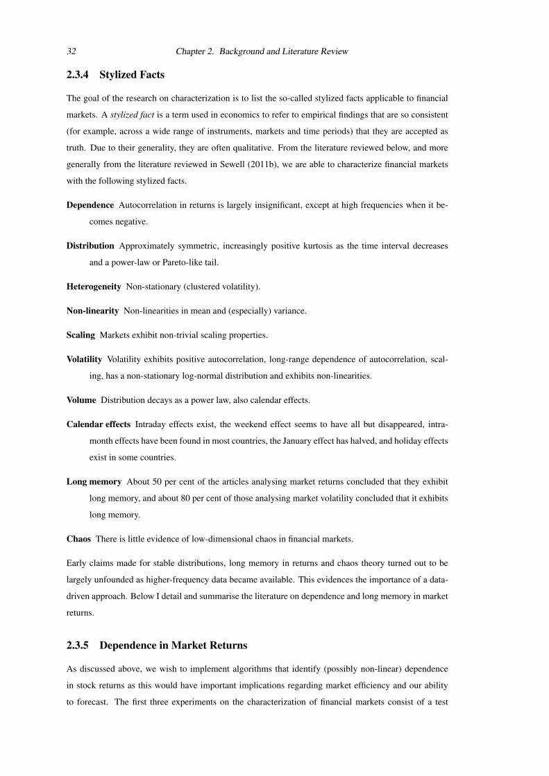
2.3.4 Stylized Facts
The goal of the research on characterization is to list the so-called stylized facts applicable to financial
markets. A stylized fact is a term used in economics to refer to empirical findings that are so consistent
(for example, across a wide range of instruments, markets and time periods) that they are accepted as
truth. Due to their generality, they are often qualitative. From the literature reviewed below, and more
generally from the literature reviewed in Sewell (2011b), we are able to characterize financial markets
with the following stylized facts.
Dependence Autocorrelation in returns is largely insignificant, except at high frequencies when it be-
comes negative.
Distribution Approximately symmetric, increasingly positive kurtosis as the time interval decreases
and a power-law or Pareto-like tail.
Heterogeneity Non-stationary (clustered volatility).
Non-linearity Non-linearities in mean and (especially) variance.
Scaling Markets exhibit non-trivial scaling properties.
Volatility Volatility exhibits positive autocorrelation, long-range dependence of autocorrelation, scal-
ing, has a non-stationary log-normal distribution and exhibits non-linearities.
Volume Distribution decays as a power law, also calendar effects.
Calendar effects Intraday effects exist, the weekend effect seems to have all but disappeared, intra-
month effects have been found in most countries, the January effect has halved, and holiday effects
exist in some countries.
Long memory About 50 per cent of the articles analysing market returns concluded that they exhibit
long memory, and about 80 per cent of those analysing market volatility concluded that it exhibits
long memory.
Chaos There is little evidence of low-dimensional chaos in financial markets.
Early claims made for stable distributions, long memory in returns and chaos theory turned out to be
largely unfounded as higher-frequency data became available. This evidences the importance of a data-
driven approach. Below I detail and summarise the literature on dependence and long memory in market
returns.
2.3.5 Dependence in Market Returns
As discussed above, we wish to implement algorithms that identify (possibly non-linear) dependence
in stock returns as this would have important implications regarding market efficiency and our ability
to forecast. The first three experiments on the characterization of financial markets consist of a test

2.3. Characterization 33
for autocorrelation and two versions of the runs test (a non-parametric statistical test of the mutual
dependence of the elements of a sequence) on a major US stock market index, so the relevant literature
on the dependence of market returns is addressed here.
Fama (1970) found that 22 out of the 30 stocks of the DJIA exhibited positive daily serial corre-
lation. Fama and French (1988) found that autocorrelations of stock return indices (they used portfo-
lios) form a U-shaped pattern across increasing return horizons. The autocorrelations become negative
for 2-year returns, reach minimum values for 3–5-year returns, and then move back towards zero for
longer return horizons. Lo and MacKinlay (1988) found significant positive serial correlation for weekly
and monthly holding-period index returns, but negative autocorrelations for individual securities with
weekly data. Ball and Kothari (1989) found negative serial correlation in five-year stock returns. Lo and
MacKinlay (1990a) found negative autocorrelation in the weekly returns of individual stocks, whilst
weekly portfolio returns were strongly positively autocorrelated. Jegadeesh (1990) found highly signifi-
cant negative serial correlation in monthly individual stock returns and strong positive serial correlation
at twelve months. Brock et al. (1992) found positive autocorrelation in DJIA daily returns. Boudoukh
et al. (1994) found that for small-firm indices, the spot index’s autocorrelation is significantly higher
than that of the futures. Zhou (1996) found that high-frequency FX returns exhibit extremely high nega-
tive first-order autocorrelation. Longin (1996) found positive autocorrelation for a daily index of stocks.
Campbell et al. (1996) reported that the autocorrelation of weekly stock returns is weakly negative, whilst
the autocorrelations of daily, weekly and monthly stock index returns are positive. Lo and MacKinlay
(1999) found a positive autocorrelation for weekly holding-period market indices returns, but a random
walk for monthly. They also found negative serial correlation for individual stocks with weekly data.
Cont (2001) found negative autocorrelation on a tick-by-tick basis for both foreign exchange (USD/JPY)
and a stock (KLM shares traded on the New York Stock Exchange (NYSE)). He also claims that weekly
and monthly autocorrelations exist. The autocorrelation of 1 minute FX returns is negative (Dacorogna
et al., 2001). Ahn et al. (2002) found that the daily autocorrelations of stock indices are nearly all posi-
tive, whilst the daily autocorrelations of the corresponding futures contracts are close to zero. Lewellen
(2002) found negative autocorrelation for stock portfolios after a year. Llorente et al. (2002) found that
the first-order autocorrelation of daily returns is negative for stocks with large bid–ask spreads (-0.088)
and small sizes (-0.076). It is positive but very small for large stocks (0.003) and stocks with small bid–
ask spreads (0.01). Bianco and Reno (2006) found negative serial correlation in the returns of Italian
stock index futures for periods smaller than 20 minutes. Cerrato and Sarantis (2006) looked at monthly
data on black market exchange rates and found evidence of non-linear mean reversion in the real ex-
change rates of developing and emerging market economies. Lim et al. (2008) examined ten Asian
emerging stock markets and discovered that all the returns series exhibit non-linear serial dependence.
Serletis and Rosenberg (2009) analysed daily data on four US stock market indices and concluded that
US stock market returns display mean reversion. Anoruo and Gil-Alana (2011) analysed stock indices
for ten African countries (daily data for four and monthly data for six) using fractionally integrated tech-
niques and found no evidence of mean reversion in any of the markets. Lim et al. (2013) analysed the

34 Chapter 2. Background and Literature Review
DJIA, S&P 500 and NYSE Composite at the daily frequency from 1970 to 2008 using the automatic
portmanteau BoxPierce test and the wild bootstrapped automatic variance ratio test, and found that those
periods with significant return autocorrelations can largely be associated with major exogenous events.
Anderson et al. (2013) found that NYSE-listed stock daily return correlations were predominantly pos-
itive for the period 1993–2000 and predominantly negative for the period 2001–2008. DeMiguel et al.
(2014) analysed the daily returns of various portfolios of US stocks between 1970 and 2011 and found
that the autocorrelations decreased with time, becoming either zero or even negative after 2008, the year
of the financial crisis.
In summary, weekly and monthly stock returns are weakly negatively correlated, whilst daily,
weekly and monthly index returns are positively correlated. Campbell et al. (1996) (p. 74) point out
that this somewhat paradoxical result can mean only one thing: large positive cross-autocorrelations
across individual securities across time. High frequency market returns exhibit negative autocorrelation.
2.3.6 Long Memory in Market Returns
An efficient market should not possess any long memory, so implementing an efficient algorithm that
tests for it is of great interest. The fourth experiment on the characterization of financial time series
concerns testing for long memory in the returns of a financial market, so the relevant literature on the
dependence of market returns is addressed here. In 1906, Harold Edwin Hurst, a young English civil
servant, came to Cairo, Egypt, which was then under British rule. As a hydrological consultant, Hurst’s
problem was to predict how much the Nile flooded from year to year. He developed a test for long-range
dependence and found significant long-term correlations among fluctuations in the Nile’s outflows and
described these correlations in terms of power laws. This statistic is known as the rescaled range, range
over standard deviation or R/S statistic. From 1951 to 1956, Hurst, then in his seventies, published a
series of papers describing his findings (Hurst, 1951). Mandelbrot (1971) showed that if asset returns
display long memory, then the impact of new market information can not be perfectly arbitraged away
and thus an efficient market becomes impossible. Mandelbrot (1972) applied R/S analysis to financial
returns. Greene and Fielitz (1977) claimed that many daily stock return series are characterized by
long-term dependence. Aydogan and Booth (1988) concluded that there was no significant evidence for
long-term memory in common stock returns.
Lo (1991) modified theR/S statistic to ensure that it is robust to short-range dependence and found
little evidence of long-term memory in historical US stock market returns. Cheung (1993) found evi-
dence of long memory in foreign exchange rates. Goetzmann (1993) considered three centuries of stock
market prices. R/S tests provided some evidence that the detrended London Stock Exchange and NYSE
prices may exhibit long-term memory. Cheung and Lai (1993) examined the long memory behaviour in
gold returns during the post-Bretton Woods period and found that the long memory behaviour in gold
returns is rather unstable. They concluded, ‘[w]hen only few observations corresponding to major po-
litical events in the Middle East, together with the Hunts event, in late 1979 are omitted, little evidence

2.3. Characterization 35
of long memory can be found.’ Mills (1993) found little evidence of long memory in daily UK stock
returns. Embrechts (1994) claims that the Hurst coefficient for JPY/USD returns indicates a memory
effect. Embrechts et al. (1994) applied rescaled range analysis to US Fed Fund rates, US Treasury notes,
CHF/USD exchange rates and the Japanese stock market (TOPIX) and claimed that it shows that most fi-
nancial markets follow a biased random walk. Bhar (1994) tested for long-term memory in the JPY/USD
exchange rate using Lo’s methodology and found no evidence of long-term memory. Moody and Wu
(1995) performed rescaled range and Hurst exponent analysis on tick-by-tick interbank foreign exchange
rates, and found that they are mean-reverting. Nawrocki (1995) considered the CRSP monthly value-
weighted index and the S&P 500 daily index, and found that the Hurst exponent and the Lo-modified
R/S statistic indicate that there is persistent finite memory. Tschernig (1995) found evidence for weak
long memory in the changes of DEM/USD spot rates and the CHF/USD spot rates; in contrast, there
was no evidence for long memory in the DEM/CHF spot rate changes. Chow et al. (1996) found evi-
dence that consistently revealed the absence of long-term dependence in 22 international equity market
indices. Moody and Wu (1996) improve Lo’s R/S statistic and conclude that the DEM/USD series is
mildly trending on time scales of 10 to 100 ticks. Peters (1996) appliedR/S analysis and concluded that
most of the capital markets are characterized by long memory processes. Lux (1996) analysed German
stock market data and found no evidence for (positive or negative) long-term dependence in the returns
series. Barkoulas and Baum (1996) applied the spectral regression method and found no evidence of long
memory in either aggregate or sectoral stock indices, but evidence of long memory in 5, intermediate
memory in 3 and no fractal structure in 22 of the 30 DJIA companies. Their overall findings did not offer
convincing evidence against the martingale model. Using the spectral regression method, Barkoulas and
Baum (1997) found significant evidence of long memory in the 3- and 6-month returns (yield changes)
on Eurocurrency deposits denominated by JPY (Euroyen). Hiemstra and Jones (1997) applied the mod-
ified rescaled range test to the return series of 1,952 common stocks and their results indicated that long
memory is not a widespread characteristic of those stocks. Lobato and Savin (1998) found no evidence
of long memory in daily stock returns. Willinger et al. (1999) found empirical evidence of long-range
dependence in stock price returns, but the evidence was not absolutely conclusive. Huang and Yang
(1999) applied the modifiedR/S technique to intraday data and found long-term memory in both NYSE
and NASDAQ indices. Baum et al. (1999) reject the hypothesis of long memory in real exchange rates
in the post-Bretton Woods era.
Using the spectral regression method, Barkoulas et al. (2000) found significant and robust evidence
of positive long-term persistence in the Greek stock market. Chen (2000) calculated Hurst’s classical
rescaled range statistic for seven Asia-Pacific countries’ stock indices and concluded that all the index
returns have long memory. Crato and Ray (2000) found no evidence for long memory in futures’ re-
turns. Weron and Przybyłowicz (2000) found that electricity price returns are strongly mean-reverting.
Zhuang et al. (2000) investigated British stock returns and found little or no evidence of long-range de-
pendence. Sadique and Silvapulle (2001) examined the presence of long memory in the weekly stock
returns of seven countries, namely Japan, Korea, New Zealand, Malaysia, Singapore, the US and Aus-

36 Chapter 2. Background and Literature Review
tralia. They found evidence for long-term dependence in four countries: Korea, Malaysia, Singapore
and New Zealand. This is consistent with more developed markets being more efficient. Cheung and
Lai (2001) found long memory in JPY-based real exchange rates. Nath (2001) found indications of long-
term memory in the Indian stock market using R/S analysis, but suggested that a more rigid analysis,
such as Lo’s modified R/S statistic, should be used. Panas (2001) found long memory in the Athens
Stock Exchange. Cavalcante and Assaf (2002) found little evidence of long memory in the returns of
the Brazilian stock market. Nath and Reddy (2002) used R/S analysis and found long-term memory
in the USD/INR exchange rate, although the variance ratio test clearly implied that there exists only
short-term memory. Henry (2002) investigated long range dependence in nine international stock index
returns. He found evidence of long memory in four of them, the German, Japanese, South Korean and
Taiwanese markets, but not for the markets of the UK, US, Hong Kong, Singapore and Australia. Tolvi
(2003a) found long memory in Finnish stock market return data. Using a monthly data set consisting of
stock market indices of 16 OECD countries, Tolvi (2003b) found statistically significant long memory
for three countries: Denmark, Finland and Ireland, which are all small markets. In a paper that examines
and compares the behaviour of four tests for fractional integration in daily observations of silver prices,
de Peretti (2003) concluded that one must use at least a bilateral bootstrap test to detect long-range de-
pendence in time series, and deduced that silver prices do not exhibit long memory. Beine and Laurent
(2003) investigated the major exchange rates and found no evidence of long memory in the conditional
mean. Limam (2003) analysed stock index returns in 14 markets and concluded that long memory tends
to be associated with thin markets. Sapio (2004) used spectral analysis and found long memory in day-
ahead electricity prices. Cajueiro and Tabak (2004) found that the markets of Hong Kong, Singapore
and China exhibit long-range dependence. Naively, Cajueiro and Tabak (2005) state that ‘the presence
of long-range dependence in asset returns seems to be a stylized fact’. They studied the individual stocks
in the Brazilian stock market and found evidence that firm-specific variables can explain, at least par-
tially, the long-range dependence phenomena. Grau-Carles (2005) applied four tests for long memory to
two major daily stock indices, the S&P 500 and the DJIA, two samples from each. There was no evi-
dence of long memory in the returns. Oh et al. (2006) studied long-term memory in various stock market
indices (using one-minute and daily data) and foreign exchange rates (using five-minute and daily data)
by applying detrended fluctuation analysis. No significant long-term memory was detected in any of
the return series. Elder and Serletis (2007) found no evidence of long memory in the DJIA. Oh et al.
(2008) studied long-term memory in two Korean stock market indices and six foreign exchange rates
using detrended fluctuation analysis. No significant long-term memory was detected in any of the return
series. Serletis and Rosenberg (2009) used daily data on four US stock market indices and concluded
that US stock market returns display anti-persistence.
Tan et al. (2010) found evidence of long memory in the Malaysian stock market before the 1997
financial crisis, but not afterwards. Kang et al. (2010) tested the daily closing prices of the KOSPI 50
index and its 50 constituent stock prices for long memory. Their broad conclusion was that there is no
long memory in the return series of the Korean stock market. Rege and Martın (2011) calculated the

2.3. Characterization 37
Hurst exponent for the Portuguese stock market and concluded that it exhibits both long-memory and
short-memory depending on the scale of the time period used. Mishra et al. (2011) used R/S analy-
sis on daily returns from the Indian stock market to reveal strong evidence of persistence or temporal
dependencies. Mukherjee et al. (2011) found no evidence for long-memory in the Indian stock market.
Anoruo and Gil-Alana (2011) examined the daily closing prices of CASE 30 (Egypt), MASI (Morocco),
TUNINDEX (Tunisia) and NSE All Share (Nigeria), and monthly data from SEM (Mauritius), NSE
20 (Kenya), JSE All Share (South Africa), ZSE Industrials (Zimbabwe), BSE (Botswana) and JSE All
Share (Namibia), and found evidence of long memory in the returns in the cases of Egypt and Nigeria,
and, to a lesser extent, for Tunisia, Morocco and Kenya. Boubaker and Makram (2012) found strong
evidence of long memory in North African stock market returns. Fouladi (2012) examined twenty-two
foreign exchange currencies vis-a-vis the Philippine peso and concluded that there was no convincing
evidence of long-term memory in any of them. Parthasarathy (2013) tested for long-range dependence in
the Indian stock market and found significant long-range dependence in all the tested indices and many
individual stocks. Yong et al. (2013) found that China’s stock market is mean reverting over the long
run and follows a long memory process. Tan et al. (2013) found no evidence of long memory for stock
returns in the Malaysian stock market. Sensoy (2013) applied generalized Hurst exponent analysis to
daily data on nineteen members of the Federation of Euro-Asian Stock Exchanges (FEAS, an interna-
tional organization comprising the main stock exchanges in Eastern Europe, the Middle East and Central
Asia) between 2007 and 2012. He deduced that in general these markets display persistent long-range
memory. Gomes et al. (2014) found slight evidence of long-term persistence in the Dutch stock market.
Kristoufek and Vosvrda (2014) analyzed 38 stock market indices across the world, the lowest Hurst ex-
ponent was 0.4470 for the FTSE in the UK, the highest was 0.6806 for the IGRA in Peru, with a mean of
0.5679. Balparda et al. (2015) found long memory in the NSE-20, the main index for the Kenyan stock
market. Sensoy and Tabak (2015) considered daily prices of all 27 stock markets in the European Union
and concluded that all stock markets have different degrees of time-varying long memory.
In summary, about half of the articles analysing stock market returns concluded that they exhibit
long memory, with the rest finding no evidence. Opinion was similarly divided for foreign exchange
returns. Some of the evidence for long memory may be due to statistical artefacts. In order to distinguish
real effects from statistical artefacts, one can ensure that the assumptions underlying any statistical tests
are valid, use as much data as possible, check for effects across subsets of data and employ more than
one test. I run the world’s only website dedicated to long-range dependence.2
2.3.7 Investment Newsletters
The fifth and final experiment on the characterization of financial time series concerns an analysis of
investment newsletters, because persistence in the ability of newsletter editors would imply that markets
are not efficient. A review of the existing literature is given here.
2http://www.long-memory.com

38 Chapter 2. Background and Literature Review
Graham and Harvey (1996) analysed the advice contained in a sample of 237 investment newsletter
strategies over 1980–1992 and found that there is little information in the investment newsletters’ opin-
ions regarding stock market direction. However they did find that the degree of disagreement among
newsletters predicts both realized and expected volatility as well as trading volume. Graham and Harvey
(1997) examined the performance of 326 newsletter asset-allocation strategies for the period 1983–1995
period. They found that, as a group, newsletters do not appear to possess any special information about
the future direction of the market. Nevertheless, they found that investment newsletters that are on a
hot streak (have correctly anticipated the direction of the market in previous recommendations) may
provide valuable information about future returns. The Value Line Investment Survey is the best known
investment newsletter, it is well-respected and freely available. Graham (1999) found that a newsletter
analyst is likely to herd on Value Line’s recommendation if his reputation is high, if his ability is low or
if the correlation across analysts’ signals is high. Jaffe and Mahoney (1999) analysed the recommenda-
tions of common stocks made by the investment newsletters followed by the Hulbert Financial Digest.
Taken as a whole, the securities that newsletters recommend did not outperform appropriate benchmarks
and the performance of the newsletters did not exhibit persistence. They found little, if any, evidence
of herding. Newsletters tend to recommend securities that have performed well in the recent past and
newsletters with poor past performance are more likely to go out of business. Metrick (1999) analysed
the equity-portfolio recommendations made by 153 investment newsletters. Overall, there was no sig-
nificant evidence of superior stock-picking ability and no evidence of abnormal short-run performance
persistence (‘hot hands’).
Kumar and Pons (2002) analysed the behaviour and performance of 353 investment newsletters
that made asset allocation recommendations during a period covering more than 21 years (June 1980–
November 2001). On aggregate the newsletters failed to outperform a passive investment strategy, but
active newsletters and contrarian newsletters exhibited market-timing ability. When they examined the
recommendations of individual newsletters at a higher frequency (daily as opposed to monthly), they
found considerable evidence of timing ability. There was also evidence of persistence in newsletters’
performance and a trading strategy that followed the average recommendations of newsletters that have
performed well in the past 10 months is capable of outperforming the market on a risk-adjusted basis (the
annual over-performance is 2.56 per cent). Brown et al. (2013) analyzed the market impact of stock rec-
ommendations made by a single investment newsletter that focuses on episodes of heavy insider trading.
The authors found that despite the fact that the recommendations are largely based on publicly available
information on insider trades and the reach of the newsletter is limited, firms identified by the newslet-
ter experience positive and statistically significant announcement period returns. Crawford et al. (2013)
found that previously strong-performing newsletters continue to outperform poor-performing newslet-
ters. This momentum was persistent and robust, using a lookback period from 1 month to 12 months.

2.4. Modelling 39
2.4 Modelling
This section is a review of the literature relevant to the experiments conducted in Chapter 4 on the
modelling of financial time series. The first experiment utilises behavioural finance, technical analysis
and multiagent systems to build an artificial stock market. The second experiment utilises prospect
theory to build a novel investment performance measurement metric.
2.4.1 Behavioural Finance
From my reading and research on behavioural finance (Sewell, 2009b, 2010a,b, 2011a; Patel and Sewell,
2015), I identified a taxonomy of heuristics and biases in the modern day investor. I summarise first then
expand.
Overconfidence is likely to lead investors to trade too much, and lead them to prefer actively managed
funds. Excess overconfidence among males in particular explains the popularity of trading among
men.
Optimism naturally creates a ‘bullish’ tendency and can create asymmetry in the behaviour of markets.
Availability could, for example, cause us to purchase shares in a company simply because it comes to
mind more readily.
Herding can lead investors to focus only on a subset of securities, whilst neglecting other securities
with near identical exogenous characteristics.
Representativeness leads analysts to believe that observed trends are likely to continue. Representative-
ness causes trend following by technical analysts and overreaction among fundamental analysts.
Anchoring is likely to cause fundamental analysts to underreact, for example to earnings announce-
ments.
I briefly review the most important literature on each in turn, plus a consequence of the biases, underre-
action and overreaction.
Overconfidence
Daniel et al. (1998) proposed a theory of security markets based on investor overconfidence (about
the precision of private information) and biased self-attribution (which causes changes in investors’
confidence as a function of their investment outcomes) which leads to market under- and overreactions.
Camerer and Lovallo (1999) found experimentally that overconfidence and optimism lead to excessive
business entry. Odean (1999) demonstrated that overall trading volume in equity markets is excessive,
and one possible explanation is overconfidence. Barber and Odean (2001) found that men trade 45 per
cent more than women and thereby reduce their returns more so than do women and conclude that this is
due to overconfidence. In Sewell (2011a) I speculate as to how overconfidence, among other heuristics
and biases, may have evolved, and focus on its effect on entrepreneurs and venture capitalists.

40 Chapter 2. Background and Literature Review
Optimism
Camerer and Lovallo (1999) found experimentally that overconfidence and optimism lead to excessive
business entry. In Sewell (2011a) I also speculate as to how optimism may have evolved.
Availability
Two psychologists, Amos Tversky and Daniel Kahneman, introduced the availability heuristic which
is a judgmental heuristic in which a person evaluates the frequency of classes or the probability of
events by the ease with which relevant instances come to mind (Tversky and Kahneman, 1973). They
explored the heuristic in a series of ten studies and demonstrated that people can assess availability with
reasonable speed and accuracy, but that the judged frequency of classes is biased by the availability of
their instances for construction and retrieval. Gilovich and Griffin (2002) included availability among
the six general purpose heuristics they identified (affect, availability, causality, fluency, similarity and
surprise). In Sewell (2011a) I also speculate as to how the availability heuristic may have evolved.
Herding
Jaffe and Mahoney (1999) analysed the recommendations of common stocks made by the investment
newsletters followed by the Hulbert Financial Digest. Taken as a whole, the securities that newsletters
recommend did not outperform appropriate benchmarks and the performance of the newsletters did not
exhibit persistence. They found little, if any, evidence of herding. Newsletters tend to recommend
securities that have performed well in the recent past and newsletters with poor past performance are
more likely to go out of business. Grinblatt et al. (1995) analysed the behaviour of mutual funds and
found evidence of momentum strategies and herding. Wermers (1999) studied herding by mutual fund
managers and he found the highest levels in trades of small stocks and in trading by growth-oriented
funds. Nofsinger and Sias (1999) found that institutional investors positive-feedback trade more than
individual investors and institutional herding impacts prices more than herding by individual investors. I
speculate as to how herding may have evolved in Sewell (2011a).
Representativeness
Kahneman and Tversky (1972) defined representativeness as when the subjective probability of an event,
or a sample, is determined by the degree to which it: (i) is similar in essential characteristics to its parent
population; and (ii) reflects the salient features of the process by which it is generated. Representative-
ness leads people to predict future events by looking for familiar patterns and taking a short history of
data and assuming that future patterns will resemble past ones. Gilovich and Griffin (2002) superseded
representativeness with attribution-substitution (prototype heuristic and similarity heuristic). In Sewell
(2011a) I also speculate as to how representativeness may have evolved.

2.4. Modelling 41
Anchoring
Tversky and Kahneman (1974) introduced anchoring and adjustment. In numerical prediction, when a
relevant value (an ‘anchor’) is available, people make estimates by starting from this anchor then make
adjustments to yield their final answer, and the adjustments are typically insufficient. We prefer relative
thinking to absolute thinking. Gilovich and Griffin (2002) superseded anchoring and adjustment with
the affect heuristic.
Underreaction and overreaction
In 1985 Werner F. M. De Bondt and Richard Thaler published ‘Does the stock market overreact?’ in the
The Journal of Finance (De Bondt and Thaler, 1985), effectively forming the start of what has become
known as behavioural finance. They discovered that people systematically overreacting to unexpected
and dramatic news events results in substantial weak-form inefficiencies in the stock market. This was
both surprising and profound. De Bondt and Thaler (1987) reported additional evidence that supports
the overreaction hypothesis. Chan et al. (1996) found that both price and earnings momentum strategies
were profitable, implying that the market responds only gradually to new information, i.e. there is un-
derreaction. Motivated by a variety of psychological evidence, Barberis et al. (1998) present a model of
investor sentiment that displays underreaction of stock prices to news such as earnings announcements
and overreaction of stock prices to a series of good or bad news. In his third review paper Fama (1998)
defends the efficient market hypothesis that he famously defined in his first, and claims that apparent
overreaction of stock prices to information is about as common as underreaction. However, this argu-
ment is unconvincing, because under- and overreactions appear to occur under different circumstances
and/or at different time intervals. Daniel et al. (1998) proposed a theory of security markets based on
investor overconfidence (about the precision of private information) and biased self-attribution (which
causes changes in investors’ confidence as a function of their investment outcomes) which leads to mar-
ket under- and overreactions. Interestingly, Veronesi (1999) presented a dynamic, rational expectations
equilibrium model of asset prices in which, among other features, prices overreact to bad news in good
times and underreact to good news in bad times. Hong and Stein (1999) modelled a market populated by
two groups of boundedly-rational agents: ‘newswatchers’ and ‘momentum traders’ which leads to under-
reaction at short horizons and overreaction at long horizons. Lee and Swaminathan (2000) showed that
past trading volume provides an important link between ‘momentum’ and ‘value’ strategies and these
findings help to reconcile intermediate-horizon ‘underreaction’ and long-horizon ‘overreaction’ effects.
2.4.2 Technical Analysis
Practitioners’ Definitions
The first three definitions below are, in spirit, consistent with my own given on p. 69, but Pring’s defini-
tion is narrower and relies on the existence of trends and reversals.
• ‘Technical analysis is the study of market action, primarily through the use of charts, for the

42 Chapter 2. Background and Literature Review
purpose of forecasting future price trends. The term “market action” includes the three principal
sources of information available to the technician—price, volume, and open interest.’ Murphy
(1999), pp. 1–2
• ‘Technical analysis is the process of analyzing a security’s historical prices in an effort to deter-
mine probable future prices.’ Achelis (2000), p. 4
• ‘It refers to the study of the action of the market itself as opposed to the study of the goods in
which the market deals. Technical Analysis is the science of recording, usually in graphic form,
the actual history of trading (price changes, volume of transactions, etc.) in a certain stock or in
“the averages” and then deducing from that pictured history the probable future trend.’ Edwards
et al. (2012), p. 5
• ‘The art of technical analysis, for it is an art, is to identify a trend reversal at a relatively early
stage and ride on that trend until the weight of the evidence shows or proves that the trend has
reversed. [. . . ] Therefore, technical analysis is based on the assumption that people will continue
to make the same mistakes they have made in the past.’ Pring (2002), p. 3
Note that technical analysis is the analysis of data generated from the activity of trading itself,
whilst fundamental analysis is the analysis of relevant news, so both are mutually exclusive subsets of
data analysis in general.
Literature Review
Brown and Jennings (1989) showed that technical analysis has value in a model in which prices are
not fully revealing and traders have rational conjectures about the relation between prices and signals.
Frankel and Froot (1990) provided evidence for the increasing use of technical analysis in the foreign
exchange markets between 1978 and 1988. Neftci (1991) showed that a few of the rules used in tech-
nical analysis generate well-defined techniques of forecasting, but even well-defined rules were shown
to be useless in prediction if the economic time series is Gaussian. However, if the processes under
consideration are non-linear, then the rules might capture some information. Tests showed that this may
indeed be the case for the moving average rule. Taylor and Allen (1992) report the results of a survey
among chief foreign exchange dealers based in London in November 1988 and found that at least 90 per
cent of respondents placed some weight on technical analysis, and that there was a skew towards using
technical, rather than fundamental, analysis at shorter time horizons. In a comprehensive and influen-
tial study Brock et al. (1992) analysed 26 technical trading rules using 90 years of daily stock prices
from the DJIA up to 1987 and found that they all outperformed the market. Blume et al. (1994) showed
that volume provides information on information quality that cannot be deduced from the price. They
also show that traders who use information contained in market statistics do better than traders who do
not. Neely (1997) explains and reviews technical analysis in the foreign exchange market. Neely et al.
(1997) used genetic programming to find technical trading rules in foreign exchange markets. The rules
generated economically significant out-of-sample excess returns for each of six exchange rates, over the

2.4. Modelling 43
period 1981–1995. Lui and Mole (1998) reported the results of a questionnaire survey conducted in
February 1995 on the use by foreign exchange dealers in Hong Kong of fundamental and technical anal-
yses. They found that over 85 per cent of respondents rely on both methods and, again, technical analysis
was more popular at shorter time horizons. Neely (1998) reconciled the fact that using technical trading
rules to trade against US intervention in foreign exchange markets can be profitable, yet, long-term, the
intervention tends to be profitable. LeBaron (1999) showed that, when using technical analysis in the
foreign exchange market, after removing periods in which the Federal Reserve is active, exchange rate
predictability is dramatically reduced.
Lo et al. (2000) examined the effectiveness of technical analysis on US stocks from 1962 to 1996
and finds that over the 31-year sample period, several technical indicators do provide incremental in-
formation and may have some practical value. Fernandez-Rodrıguez et al. (2000) applied an artificial
neural network (ANN) to the Madrid Stock Market and find that, in the absence of trading costs, the
technical trading rule is always superior to a buy-and-hold strategy for both ‘bear’ market and ‘stable’
market episodes, but not in a ‘bull’ market. One criticism I have is that beating the market in the absence
of costs seems of little significance unless one is interested in finding a signal which will later be incor-
porated into a full system. Secondly, it is perhaps naive to work on the premise that ‘bull’ and ‘bear’
markets exist, statistically. Lee and Swaminathan (2000) demonstrated the importance of past trading
volume. Neely and Weller (2001) used genetic programming to show that technical trading rules can
be profitable during US foreign exchange intervention. Cesari and Cremonini (2003) made an extensive
simulation comparison of popular dynamic strategies of asset allocation and found that technical analy-
sis only performs well in Pacific markets. Cheol-Ho Park and Scott H. Irwin wrote ‘The profitability of
technical analysis: A review’ (Park and Irwin, 2004), a very thorough review paper on technical analy-
sis. Kavajecz and Odders-White (2004) showed that support and resistance levels coincide with peaks
in depth on the limit order book3 and moving average forecasts reveal information about the relative
position of depth on the book. They also show that these relationships stem from technical rules locating
depth already in place on the limit order book. In their book, The Evolution of Technical Analysis, Lo and
Hasanhodzic (2010) provide a comprehensive history of the evolution of technical analysis from ancient
times to the Internet age.
I host and run a website dedicated to technical analysis which, unusually, has an academic flavour.4
Conclusions
Publication bias (discussed on p. 110) should not adversely affect the relative performance of technical
analysis, such as comparing different techniques, or their efficacy in different markets. The review paper
by Park and Irwin (2004) does precisely that. The above literature review together with Park and Irwin’s
results give rise to the following conclusions:
• There is evidence in support of the usefulness of moving averages, momentum, support and resis-3A limit order is an order to a broker to buy(sell) a security at or below(above) a specific price; whilst a limit order book is a
record of unexecuted limit orders maintained by the specialist.4http://www.technicalanalysis.org.uk

44 Chapter 2. Background and Literature Review
tance and some patterns; but no convincing evidence in support of Gann Theory or Elliott Wave
Theory.5
• Technical analysis works best on currency markets, intermediate on futures markets, and worst on
stock markets. An explanation is given on p. 114.
• Chart patterns work better on stock markets than currency markets.
• Non-linear methods work best overall. This is not at all surprising in light of the non-linearities
found in markets (Hsieh, 1989; Scheinkman and LeBaron, 1989; Brock et al., 1991).
• Technical analysis doesn’t work as well as it used to. As transaction costs decrease, available
computing power increases and the number of market participants increases, one would expect
markets to become increasingly efficient and thus it is not surprising that the efficacy of technical
analysis should diminish.
2.4.3 Multiagent Systems
The artificial stock market in Chapter 4 employs a multiagent system, which is defined and the concept
criticised in Section 4.1.1 (p. 65). Two good books on multiagent systems are Wooldridge (2009) and
Weiss (2013). In a classic paper, Arthur et al. (1997) proposed a theory of asset pricing based on hetero-
geneous agents who continually adapt their expectations to the market that these expectations aggrega-
tively create, thus creating an artificial stock market. LeBaron (2006) surveys research on agent-based
models used in finance. Martinez-Jaramillo (2007) and Martinez-Jaramillo and Tsang (2009) developed
an artificial financial market and modelled technical, fundamental and noise traders. They investigated
the different conditions under which the statistical properties of an artificial stock market resemble those
of a real financial market, and investigated the effects on the market when the agents learn. Railsback
(2001) addresses the problem of getting ‘results’—general principles and conclusions—from multiagent
systems and recommends a pattern-oriented approach.
2.4.4 Prospect Theory
From the field of economics, expected utility theory (also known as von Neumann-Morgenstern utility)
(Bernoulli, 1738; von Neumann and Morgenstern, 1944; Bernoulli, 1954) is a normative model of de-
cision making under risk. Expected utility theory states that when making decisions under risk people
choose the option with the highest utility, where utility is the sum of the products of the utility of each
potential outcome and the probability of occurrence of the outcome.
The most cited paper ever to appear in Econometrica, the prestigious academic journal of eco-
nomics, was written by the two psychologists Kahneman and Tversky (1979). They present a critique of
5For details of traditional technical analysis, see Murphy (1999), Achelis (2000), Edwards et al. (2012) and Pring (2014). There
is money to be made selling books on technical analysis. Caveat emptor! The eminently more sensible Aronson (2006) offers a
glimmer of hope.

2.4. Modelling 45
expected utility theory as a descriptive model of decision making under risk and develop an alternative
model, which they call ‘prospect theory’. Prospect theory is a descriptive model of decision making
under risk. Kahneman and Tversky found empirically that people underweight outcomes that are merely
probable in comparison with outcomes that are obtained with certainty; also that people generally dis-
card components that are shared by all prospects under consideration. Under prospect theory, value
is assigned to gains and losses rather than to final assets; also probabilities are replaced by decision
weights. Decision weights are inferred from choices between prospects much as subjective probabilities
are inferred from preferences in the subjective interpretation of probability. The value function is defined
on deviations from a reference point and is normally concave for gains (implying risk aversion), com-
monly convex for losses (risk seeking) and is generally steeper for losses than for gains (loss aversion)
(see Figure 2.1). Decision weights are generally lower than the corresponding probabilities, except in
the range of low probabilities. The theory—which they confirmed by experiment—predicts a distinctive
fourfold pattern of risk attitudes: risk aversion for gains of moderate to high probability and losses of
low probability, and risk seeking for gains of low probability and losses of moderate to high probability.
Note that there are two fundamental reasons why prospect theory (which calculates value) is inconsis-
-2
-1
0
1
2
-2 -1 0 1 2Valu
e
Losses Value Gains
Figure 2.1: A hypothetical value function in prospect theory
tent with expected utility theory. Firstly, whilst utility is necessarily linear in the probabilities, value is
not. Secondly, whereas utility is dependent on final wealth, value is defined in terms of gains and losses
(deviations from current wealth).
Thaler (1980) argues that there are circumstances when consumers act in a manner that is inconsis-
tent with economic theory and he proposes that Kanneman and Tversky’s prospect theory be used as the
basis for an alternative descriptive theory. Tversky and Kahneman (1986) argue that, due to framing and
prospect theory, the rational theory of choice does not provide an adequate foundation for a descriptive
theory of decision making.
Tversky and Kahneman (1992) superseded their original implementation of prospect theory with

46 Chapter 2. Background and Literature Review
cumulative prospect theory. The new methodology employs cumulative rather than separable decision
weights, applies to uncertain as well as to risky prospects with any number of outcomes, and it allows
different weighting functions for gains and for losses (see Figure 2.2). I have developed a cumulative
0
0.1
0.2
0.3
0.4
0.5
0.6
0.7
0.8
0.9
1
0 0.1 0.2 0.3 0.4 0.5 0.6 0.7 0.8 0.9 1
w(p
)
p
w+
w-
Figure 2.2: Typical probability weighting functions for gains (w+) and losses (w−) in cumulative prospect theory
prospect theory calculator, which is freely available online for the Web and Excel.6
More recent developments in decision making under risk have improved upon cumulative prospect
theory, such as the transfer of attention exchange model (Birnbaum and Chavez, 1997). Kahneman and
Tversky (2000) edited the book Choices, Values, and Frames, which presents a selection of the research
that grew from their collaboration on prospect theory. Barberis et al. (2001) incorporated prospect theory
in a model of asset prices in an economy. Daniel Kahneman won the 2002 Bank of Sweden Prize in
Economic Sciences in Memory of Alfred Nobel for his work on prospect theory, despite being a research
psychologist and not an economist. If it were not for his untimely death, Amos Tversky, Kahneman’s
collaborator, would have almost certainly shared the prize. In Sewell (2009b) I explain that a responsible
investment manager should seek a compromise between the normative expected utility theory and the
prescriptive prospect theory, and call for a prescriptive model of risk preferences. Harrison and Rutstrom
(2009) proposed a reconciliation of expected utility theory and prospect theory by using a mixture model.
Wakker (2010) wrote the first book on prospect theory, it covers decision making under both known and
unknown probabilities, and includes expected utility, rank-dependent utility and prospect theory.
2.4.5 Investment Performance Measurement
The secondary piece of research in Chapter 4 concerns investment performance measurement. Popu-
lar investment performance metrics include the Sharpe ratio (Sharpe, 1994), Sortino ratio (Sortino and
van der Meer, 1991) and (less common) Omega (Shadwick and Keating, 2002). Omega has the advan-
6http://prospect-theory.behaviouralfinance.net

2.5. Forecasting 47
tage that it captures all of the moments of the returns distribution. Goetzmann et al. (2002) proved that
an optimal (high) Sharpe ratio strategy would produce a distribution with a truncated right tail and a fat
left tail.
2.5 Forecasting
This section is a review of the literature relevant to the experiments conducted in Chapter 5 on the fore-
casting of financial time series. It consists of an explanation of the no free lunch theorem for supervised
machine learning, a review of the literature on data snooping, a note on kernel methods, a review of
the literature that concerns the prediction of financial or commodity markets and compares SVMs with
ANNs, and a brief review of genetic programming because my forecasting with kernel methods is com-
pared with a genetic programming approach.
2.5.1 No Free Lunch Theorem for Supervised Machine Learning
The no free lunch theorem (NFL) for supervised machine learning is non-trivial, frequently misunder-
stood and profoundly relevant to machine learning and science in general (and often conveniently ignored
by the machine learning communities).
Hume (1739–40) pointed out that ‘even after the observation of the frequent or constant conjunction
of objects, we have no reason to draw any inference concerning any object beyond those of which
we have had experience’. More recently, and with increasing rigour, Mitchell (1980), Schaffer (1994)
and Wolpert (1996) showed that bias-free learning is futile. The no free lunch theorem for supervised
machine learning (Wolpert, 1996) shows that in a noise-free scenario where the loss function is the
misclassification rate, in terms of off-training-set error, there are no a priori distinctions between learning
algorithms.
More formally, where
d = training set;
m = number of elements in training set;
f = ‘target’ input-output relationships;
h = hypothesis (the algorithm’s guess for f made in response to d); and
c = off-training-set ‘loss’ associated with f and h (‘generalization error’ or ‘test set error’)
all algorithms are equivalent, on average, by any of the following measures of risk: E(c|d), E(c|m),
E(c|f, d) or E(c|f,m).
How well you do is determined by how ‘aligned’ your learning algorithm P (h|d) is with the actual
posterior, P (f |d). This result, in essence, formalizes Hume, extends him and calls all of science into
question.
This foray into the no free lunch theorem for supervised machine learning is to place the work in this
thesis in context: we cannot make any general claims about the superiority or otherwise of the algorithms
used or developed, at best we can claim that they are well suited to the data sets employed here. The

48 Chapter 2. Background and Literature Review
key to developing successful machine learning algorithms is to carefully consider the assumptions being
made, which requires extracting as much domain knowledge as possible. I run the world’s only No Free
Lunch website.7
2.5.2 Data Snooping
Data snooping (also known as data dredging and (confusingly, in economics) data mining) occurs when
a set of data is used more than once for purposes of inference or model selection. This can lead to
biases. When data mining, one has to take into account the fact that one is data mining, also that
one has read papers that may have been written on the basis of inferences from the same data set that
one’s own work is based on. For example, the S&P 500 has been the subject of an enormous number
of studies. Lo and MacKinlay (1990b) noted that tests of financial asset pricing models may yield
misleading inferences when properties of the data are used to construct the test statistics. ‘In particular,
such tests are often based on returns to portfolios of common stock, where portfolios are constructed
by sorting on some empirically motivated characteristic of the securities such as market value of equity.
Analytical calculations, Monte Carlo simulations, and two empirical examples show that the effects of
this type of data snooping can be substantial.’ In 2000, Halbert White published ‘A reality check for data
snooping’ (White, 2000). He specified a new procedure, the ‘Reality Check’, which is a straightforward
procedure for testing the null hypothesis that the best model encountered in a specification search has
no predictive superiority over a given benchmark model, permitting account to be taken of the effects of
data snooping. White claims that his method ‘permits data snooping to be undertaken with some degree
of confidence that one will not mistake results that could have been generated by chance for genuinely
good results’. Sullivan et al. (1999) utilized White’s Reality Check bootstrap methodology to evaluate
simple technical trading rules while quantifying the data-snooping bias and fully adjusting for its effect
in the context of the full universe from which the trading rules were drawn. Aronson (2006) suggests
three approaches for dealing with data mining bias. His first, out-of-sample testing, involves excluding
one or more subsets of the historical data from the data mining, as used in this thesis. His second
approach, randomization methods, includes methods like bootstrapping and the Monte Carlo method.
His third suggestion, a data-mining correction factor developed by Markowitz and Xu (1994), deflates
the observed performance of the rule that did the best. In theory the best approach of all would be to use
Bayesian model selection, as outlined in the pedagogical example I wrote for Futures magazine (Sewell,
2009a).
2.5.3 Kernel Methods
Central to the work on forecasting in Chapter 5 is the concept of a kernel. The technical aspects of
kernels are dealt with in Section 5.2 (pp. 84–85), and the history is given here. Also, the Fisher kernel is
derived and implemented in Chapter 5; to save space, a thorough literature review is provided in Sewell
(2011g).
7http://www.no-free-lunch.org

2.5. Forecasting 49
2.5.4 Support Vector Machines
Support vector machines (SVMs) are used in the forecasting of financial time series and are covered in
more detail in Section 5.3 (p. 85). Among other sources, the introductory paper (Hearst et al., 1998),
the classic SVM tutorial (Burges, 1998), the book (Cristianini and Shawe-Taylor, 2000) and the imple-
mentation details within Joachims (2002) have contributed to my own understanding. Below I review
the literature that concerns the prediction of financial or commodity markets and compares SVMs with
ANNs.
Trafalis and Ince (2000) compared two SVMs for regression (one implementing a primal-dual inte-
rior point quadratic programing (QP) algorithm and the other a standard QP algorithm) and two artificial
neural networks (ANNs) (a backpropagation multilayer perceptron (MLP) and a radial basis function
(RBF) network) by predicting IBM, Yahoo and America Online daily stock prices. Oddly, they forwent
a validation set, and with the SVMs, set ε to zero, fixed C and repeated the experiment for various
fixed settings of the kernel parameter, σ, giving rise to several results. By considering either the best
results or the average results for each of the four methods, the ranking was the same, from best to worst
performance: 1st MLP, 2nd RBF, 3rd primal-dual SVM and 4th standard SVM.
Cao and Tay (2001) found that SVMs forecast the S&P 500 daily price index better than a mul-
tilayer perceptron trained by the backpropagation algorithm. Tay and Cao (2001) found that an SVM
outperformed a multilayer backpropagation ANN on five real futures contracts, the S&P 500 stock index
futures (CME-SP), US 30-year government bond (CBOT-US), US 10-year government bond (CBOT-
BO), German 10-year government bond (EUREX-BUND) and French government stock index futures
(MATIF-CAC40).
Abraham et al. (2002) analysed the performance of an ANN trained using the Levenberg-Marquardt
algorithm, an SVM, a Takagi-Sugeno neuro-fuzzy model and a difference boosting neural network
(DBNN) when predicting the NASDAQ-100 and the S&P CNX Nifty. There was no clear winner.
Sansom et al. (2003) evaluated utilizing ANNs and SVMs for wholesale (spot) electricity price
forecasting. The SVM required less time to optimally train than the ANN, whilst the SVM and ANN
forecasting accuracies were found to be very similar. Similar to Abraham et al. (2002), Abraham et al.
(2003) applied four different techniques, an ANN trained using the Levenberg-Marquardt algorithm, an
SVM, a difference boosting neural network and a Takagi-Sugeno fuzzy inference system learned using
an ANN algorithm (neuro-fuzzy model) to the prediction of the NASDAQ-100 and the S&P CNX Nifty.
No one technique was clearly superior, but absurdly, they attempted to predict the absolute value of
the indices, rather than use log returns. Similar to Abraham et al. (2002) and Abraham et al. (2003),
Abraham and AuYeung (2003) considered an ANN trained using the Levenberg-Marquardt algorithm,
an SVM, a Takagi-Sugeno neuro-fuzzy model and a difference boosting neural network for predicting the
NASDAQ-100 and the S&P CNX Nifty. They concluded that an ensemble of the intelligent paradigms
performed better than the individual methods. The SVM outperformed the ANN. Kim (2003) found
that SVMs outperformed backpropagation ANNs and case-based reasoning when used to forecast the
daily Korea Composite Stock Price Index (KOSPI). Cao and Tay (2003) used an SVM, a multilayer

50 Chapter 2. Background and Literature Review
backpropagation (BP) ANN and a regularized radial basis function (RBF) ANN to predict five real
futures contracts collated from the Chicago Mercantile Exchange. Results showed that the SVM and the
regularized RBF ANN were comparable and both outperformed the BP ANN, with the SVM being best.
Ince and Trafalis (2004) found that MLP ANNs outperform support vector regression when applied
to stock price prediction.
Chen and Ho (2005) used an SVM for regression for forecasting the Taiwan Stock Exchange Cap-
italization Weighted Stock Index. Oddly, they considered price, rather than returns. The results demon-
strated that the SVM outperformed the backpropagation ANN and random walk models. Huang et al.
(2005) compared the ability of SVMs, linear discriminant analysis, quadratic discriminant analysis and
Elman backpropagation ANNs to forecast the weekly movement direction of the Nikkei 225 index and
found that the SVM outperformed all of the other classification methods. Better still was a weighted
combination of the models.
Yu et al. (2006) applied a random walk (RW) model, an autoregressive integrated moving average
(ARIMA) model, an individual backpropagation ANN model, an individual SVM model and a genetic
algorithm-based SVM (GASVM) to the task of predicting the direction of change in the daily S&P 500
stock price index and found that their proposed GASVM model performed the best, and the SVM sec-
ond best. Chen et al. (2006) compared SVMs and backpropagation (BP) ANNs when forecasting the six
major Asian stock markets. Both models performed better than the benchmark AR(1) model in the devi-
ation measurement criteria, whilst SVMs performed better than the BP model in four out of six markets.
Pai et al. (2006) developed a hybrid SVM model composed of a linear SVM and a non-linear SVM, fur-
thermore the parameters of both were determined by genetic algorithms. Their approach outperformed
an ANN, a chaotic model (vector-valued, local linear approximation) and a random walk model when
predicting exchange rates. Xie et al. (2006) compared SVMs with ARIMA and a backpropagation ANN
for crude oil price prediction; the SVM outperformed the other two methods.
Wu et al. (2007) used a real-valued genetic algorithm to optimize the parameters C and σ of an
SVM for predicting bankruptcies in Taiwan. Their method achieved better predictive accuracy than a
traditional SVM, discriminant analysis, logit analysis, probit regression and a feed-forward backpropa-
gation ANN. The traditional SVM beat the ANN on the holdout sample. Sai et al. (2007) used rough
sets for feature selection with an SVM for classification to predict the daily CSI 300 Index. Their model
outperformed a random walk model, an ARIMA model, a backpropagation ANN and a standard SVM,
with the standard SVM being the second best.
Xin and Gu (2008) describe a method based on the least squares SVM, which changes the inequality
restriction in the traditional SVM into an equality restriction and uses the loss function of the quadratic
sum of the errors as the empirical function for the training set. The quadratic programming problem is
converted into one of solving linear equations, which significantly improves the training speed and the
convergence accuracy. By way of example, the authors used their method to successfully predict a stock
index, which resulted in faster training time and better accuracy than an ANN model. Ince and Trafalis
(2008) used an SVM for regression and a multilayer perceptron ANN to predict daily stock prices of ten

2.5. Forecasting 51
companies traded on the NASDAQ, and compared the results with ARIMA. On average, the SVM was
the better technique.
Yu et al. (2009) used a genetic algorithm (GA) to select input features, and another GA for parameter
optimization, for a least squares SVM applied to the classification of monthly S&P 500, DJIA and NYSE
returns. Their method was superior to an autoregressive integrated moving average (ARIMA) model, a
linear discriminant analysis (LDA) model, a backpropagation ANN and a standard SVM. The standard
SVM beat the ANN.
Zeng-min and Chong (2010) used an SVM and a three-layer fully connected backpropagation neural
network (BNN) to forecast the S&P 500 and the Nikkei 225, and found that the SVM outperformed the
BNN. Huang et al. (2010) implemented a chaos-based SVM for regression applied to daily exchange
rate forecasting of EUR/USD, GBP/USD, NZD/USD, AUD/USD, JPY/USD and RUB/USD. Firstly, the
delay coordinate embedding was used to reconstruct the unobserved phase space (or state space) of the
exchange rate dynamics, then an SVM was used for forecasting. Their proposed method performed
better than traditional ANNs, traditional SVMs or chaos-based ANNs. The traditional SVM ranked
second.
Yeh et al. (2011) forecast the Taiwan Capitalization Weighted Stock Index (TAIEX) using multiple-
kernel support vector regression (MKSVR), single kernel support vector regression (SKSVR) and TSK
type fuzzy neural network (FNN). The FNN was inferior to the SVMs. Kara et al. (2011) used an ANN
and an SVM to predict the direction of movement in the daily Istanbul Stock Exchange (ISE) National
100 Index. The average performance of the ANN model was found to be significantly better than that of
the SVM model.
Timor et al. (2012) used SVMs and ANNs to forecast the Istanbul Stock Exchange (ISE) National-
30 and on average the ANNs were superior. Das and Padhy (2012) used a backpropagation neural
network and an SVM for regression to predict the price of futures traded on the Indian stock market.
The SVM outperformed the ANN in most of the cases. Hajek (2012) used various prototype generation
classifiers, ANNs and SVMS to predict the trend of the NASDAQ Composite index. There was no
significant difference in the performance across the ANNs and SVMs.
Kazem et al. (2013) applied a genetic algorithm-based SVR (SVR-GA), a chaotic genetic algorithm-
based SVR (SVR-CGA), a firefly-based SVR (SVR-FA), an artificial neural network (ANN) and an
adaptive neuro-fuzzy inference systems (ANFIS) to forecasting the price of three stocks from NASDAQ,
namely Intel, National Bankshares and Microsoft. The SVR-CFA performed the best, the SVR-CGA the
second worst and the SVR-GA the worst.
Zhu and Wei (2013) forecast carbon futures prices using ARIMA, a least squares SVM (LSSVM)
an ANN and hybrid models, and the SVMs outperformed the ANNs (both on their own and when com-
bined with ARIMA). Mantri (2013) used an SVM and a multilayer perceptron ANN to forecast the BSE
SENSEX, and the SVM proved to be superior.
Li et al. (2014) compared a basic extreme learning machine (a single hidden layer feedforward
neural network with random hidden nodes) (ELM), an RBF kernel-based extreme learning machine (K-

52 Chapter 2. Background and Literature Review
ELM), a back-propagation neural network (BP-NN) and an RBF support vector machine (SVM) for
forecasting intraday stock prices of stocks from the H share market (the shares of companies incorpo-
rated in mainland China that are traded on the Hong Kong Stock Exchange). Both the K-ELM and the
SVM achieved higher prediction accuracy and faster prediction speed than the BP-NN and the basic
version of the ELM. Okasha (2014) used ARIMA, ANN and SVM models to forecast the Al-Quds In-
dex, the primary stock index of the Palestine Securities Exchange, and found that the SVM performed
significantly better than ARIMA and the ANN.
Deng et al. (2015) combined multiple kernel learning for regression and a genetic algorithm to con-
struct trading rules for forecasting short-term foreign exchange rates. Their proposed hybrid method out-
performed other baseline methods in terms of returns and return-risk ratio. On average, the SVM-based
techniqes outperformed the ANN. Patel et al. (2015) forecast the CNX Nifty and S&P BSE SENSEX
Indian stock markets 1–10, 15 and 30 days ahead using an ANN, Random Forest and SVR, along with
three two-stage fusion approaches, SVRANN, SVRRandom Forest and SVRSVR. The SVRANN and
SVRSVR performed best, and the ANN and Random Forest performed the worst. Thakare and Samb-
hare (2015) used an SVM and an ANN to classify stocks, and found the SVM to be superior to the
ANN.
Of the 36 articles above that concern the prediction of financial or commodity markets and compare
SVMs with ANNs, SVMs outperformed ANNs in 28 cases, ANNs outperformed SVMs in 4 cases, and
there was no significance difference in 4 cases. Furthermore, Sapankevych and Sankar (2009) present
a general survey of SVM applications to time series prediction, and summarize 66 papers. Financial
market prediction was the most studied application (21 papers). This bodes well for SVMs, and as such,
the research on forecasting shall employ them. The reason that SVMs more often than not outperformed
ANNs when forecasting financial time series could be that they are less prone to overfitting. Note that
whilst kernels allow SVMs to define non-linear decision boundaries, neural networks also define non-
linear decision boundaries. Most of the SVMs in the above literature employed the generic RBF kernel,
so it is difficult to draw conclusions regarding the optimal choice of kernel.
2.5.5 Genetic Programming
In the Chapter on forecasting my work is compared with the genetic programming approach used in
Neely et al. (1997) and reported in Neely et al. (2009), so we consider genetic programming here. Ge-
netic programming (GP) is an evolutionary algorithm that optimizes a population of computer programs
according to a fitness landscape determined by a program’s ability to perform a user-defined task. The
first experiments with GP were reported by Smith (1980) and Cramer (1985), and the seminal book
is Koza (1992). On average, GP is no better or worse than any other search/optimization algorithm
(Wolpert and Macready, 1997). Neely et al. (1997) used genetic programming to find technical trad-
ing rules for six exchange rates over the period 1981–1995 and found strong evidence of economically
significant out-of-sample excess returns. The model space they employed incorporated trading rules
including moving average rules and filter rules. A meta-analysis by Park and Irwin (2004) found that ge-

2.5. Forecasting 53
netic programming worked well on currency markets, but performed poorly on stock markets and futures
markets.

54 Chapter 2. Background and Literature Review

55
Chapter 3
Characterization
The current plus the following two chapters (chapters 3, 4 and 5) make up the core of the
thesis and contain the bulk of the contributions. The work in the present chapter seeks to
extend the literature on the characterization of financial time series. This chapter describes
five experiments, each of the first four analyse daily, weekly, monthly and annual data from
a major US stock market index. The experiments are chosen because they are tests of market
efficiency, and help us to characterize financial markets. The first and most straightforward
is a measurement of the autocorrelation of stock market returns. For the following three
experiments, two pieces of software are written, a program for performing two versions
of the runs test and a program for testing for the existence of long memory, and both are
used to analyse the dependence of stock market returns. The fifth experiment involves the
analysis of the performance of investment newsletters. All five experiments (potentially)
have implications apropos market efficiency. The characterization of financial time series
provides us with the all-important domain knowledge that machine learning, employed in
the chapter on forecasting, relies upon. This chapter is published as Sewell (2012a).
3.1 Data
The first four experiments in this chapter (autocorrelation, two versions of the runs test and long memory)
use data from the Dow Jones Industrial Average (DJIA). The Dow is the best-known US stock index, and
the second-oldest (after the Dow Jones Transportation Average). The index is a price-weighted1 aver-
age (rather than a market-value weighted or capitalization-weighted index) of 30 large, publicly-owned
companies based in the US. The DJIA daily closing prices from 1 October 1928 to 23 March 2012
were downloaded from Yahoo! Finance. The analyses were conducted independently on daily, weekly,
monthly and annual log returns, as a truly efficient market should pass tests of efficiency at all time
intervals. Returns, rather than price, are used as some of the statistical tests require a stationary variable.
Although the Dow represents the average of its constituent stocks, care should be taken when extrap-
1Each constituent makes up a fraction of the index that is proportional to its price.

56 Chapter 3. Characterization
olating the characteristics of a stock index to the characteristics of individual stocks. For example, as
pointed out on p. 34, although weekly and monthly stock returns are weakly negatively correlated, daily,
weekly and monthly index returns are positively correlated, due to large positive cross-autocorrelations
across individual securities across time. The first three experiments (autocorrelation and two versions
of the runs test) are also applied to foreign exchange data (the currency pairs USD/DEM, USD/JPY,
GBP/USD, USD/CHF, DEM/JPY, GBP/CHF). The fifth investigation employs data from an analysis of
investment newsletters, ‘The Forbes/Hulbert investment letter survey’ (Hulbert, 2002).
The no free lunch theorem (NFL) for supervised machine learning (Section 2.5.1 (p. 47)) informed
us that the key to developing successful forecasting algorithms is to extract as much domain knowledge
as possible. However, the dangers of data snooping (Section 2.5.2 (p. 48)) mean that we should take
care to avoid viewing any out-of-sample data before forecasting. These are conflicting requirements,
as the more data used to gain domain knowledge, the less is available for out-of-sample testing. So
two strategies have been adopted. The characterisation of the DJIA was done before forecasting, whilst
the foreign exchange data was characterised after the forecasting, in order to reflect on why certain
algorithms worked better than others.
3.2 Autocorrelation
A necessary (but not sufficient) condition for the martingale hypothesis to hold is that the time series
has no autocorrelation of any order. Let X be a stochastic process and t a point in time, then Xt is the
realisation produced by a given run of the process at time t. Suppose that X has mean µt and variance
σ2t at time t, for each t. Then the autocorrelation between times s and t is defined by
R(s, t) =E[(Xt − µt)(Xs − µs)]
σtσs, (3.2.1)
where ‘E’ is the expected value operator. Note that due to the definition of autocorrelation, detrending
data is not necessary (the results will be the same). Note also that autocorrelation is sensitive only to
linear relationships.
The first-order autocorrelation of DJIA and foreign exchange log returns are measured using Mi-
crosoft Excel. Table 3.1 (p. 57) shows the autocorrelation of daily, weekly, monthly and annual DJIA
log returns. Autocorrelation is small but positive for all time periods. The autocorrelations for daily and
weekly returns are the closest to zero, and thus (potentially) an efficient market.
Table 3.2 (p. 57)) shows the autocorrelation of foreign exchange daily log returns. They are also
small and positive, but significantly larger than the autocorrelation for DJIA daily log returns. The
autocorrelation is smallest for the currency pair USD/CHF, and largest for DEM/JPY and GBP/USD.
The results suggest that the foreign exchange market is less efficient than the DJIA, which is to be
expected. As explained in Table 2.1 (p. 31), due to risk aversion, because markets are risky investors
require a small positive expected return. A stock market, in general, is long-only, which implies a positive
upward drift. Foreign exchange markets are symmetric, traders are as likely to be long as they are short,
which implies that one would expect the price to be predictable to some degree.

3.3. Runs Test 57
Table 3.1: Autocorrelation of DJIA log returns
Time interval Autocorrelation
Daily 0.0138
Weekly 0.0117
Monthly 0.0793
Annual 0.1194
Table 3.2: Autocorrelation of foreign exchange log returns
Time interval Autocorrelation
USD/DEM 0.0403
USD/JPY 0.0434
GBP/USD 0.0693
USD/CHF 0.0307
DEM/JPY 0.0614
GBP/CHF 0.0403
3.3 Runs Test
As tests for weak-form market efficiency Aumeboonsuke and Dryver (2014) compared the runs test,
the autocorrelation test and the variance ratio test. They concluded that it is best to use a test that does
not require data snooping, for example the runs test (which does not require any parameters). In their
simulation, the runs test had the lowest type I error (rejecting market efficiency when it is true), but never
had the highest power in any of the scenarios.
The runs test is a non-parametric statistical test that can be used to test for serial dependence, a lack
of dependence being a necessary (but not sufficient) condition for the martingale hypothesis to hold. A
‘run’ within a sequence is a maximal non-empty consecutive subsequence consisting of adjacent equal
elements. For example, the sequence ‘+ − − − + − + + + + −+’ consists of seven runs. In contrast
to autocorrelation, the runs test loses information because the magnitude of the returns is lost. However,
whilst autocorrelation can detect only linear relationships, the runs test can detect both linear and non-
linear relationships. The runs test assumes that the sequence is not only uncorrelated, but also serially
independent and identically distributed. If a sequence has zero mean, the runs test becomes a direct
test of a martingale. For both of the runs tests described below, there is no need to detrend the data,
nor is it necessary to assume that the ‘+’s and ‘−’s have equal probabilities, the tests only assume that
the elements are independent and identically distributed. If the number of runs is significantly higher
or lower than expected, the hypothesis of statistical independence may be rejected. Both runs tests are
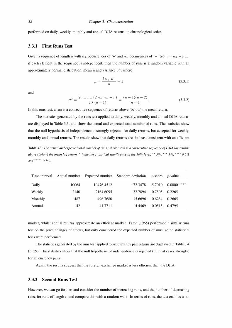
58 Chapter 3. Characterization
performed on daily, weekly, monthly and annual DJIA returns, in chronological order.
3.3.1 First Runs Test
Given a sequence of length n with n+ occurrences of ‘+’ and n− occurrences of ‘−’ (so n = n+ +n−),
if each element in the sequence is independent, then the number of runs is a random variable with an
approximately normal distribution, mean µ and variance σ2, where
µ =2 n+ n−
n+ 1 (3.3.1)
and
σ2 =2 n+ n− (2 n+ n− − n)
n2 (n− 1)=
(µ− 1)(µ− 2)
n− 1. (3.3.2)
In this runs test, a run is a consecutive sequence of returns above (below) the mean return.
The statistics generated by the runs test applied to daily, weekly, monthly and annual DJIA returns
are displayed in Table 3.3, and show the actual and expected total number of runs. The statistics show
that the null hypothesis of independence is strongly rejected for daily returns, but accepted for weekly,
monthly and annual returns. The results show that daily returns are the least consistent with an efficient
Table 3.3: The actual and expected total number of runs, where a run is a consecutive sequence of DJIA log returns
above (below) the mean log return. ∗ indicates statistical significance at the 10% level, ∗∗ 5%, ∗∗∗ 1%, ∗∗∗∗ 0.5%
and ∗∗∗∗∗ 0.1%.
Time interval Actual number Expected number Standard deviation z-score p-value
Daily 10064 10476.4512 72.3478 -5.7010 0.0000∗∗∗∗∗
Weekly 2140 2164.6095 32.7894 -0.7505 0.2265
Monthly 487 496.7680 15.6696 -0.6234 0.2665
Annual 42 41.7711 4.4469 0.0515 0.4795
market, whilst annual returns approximate an efficient market. Fama (1965) performed a similar runs
test on the price changes of stocks, but only considered the expected number of runs, so no statistical
tests were performed.
The statistics generated by the runs test applied to six currency pair returns are displayed in Table 3.4
(p. 59). The statistics show that the null hypothesis of independence is rejected (in most cases strongly)
for all currency pairs.
Again, the results suggest that the foreign exchange market is less efficient than the DJIA.
3.3.2 Second Runs Test
However, we can go further, and consider the number of increasing runs, and the number of decreasing
runs, for runs of length i, and compare this with a random walk. In terms of runs, the test enables us to

3.3. Runs Test 59
Table 3.4: The actual and expected total number of runs, where a run is a consecutive sequence of foreign exchange
log returns above (below) the mean log return. ∗ indicates statistical significance at the 10% level, ∗∗ 5%, ∗∗∗ 1%,∗∗∗∗ 0.5% and ∗∗∗∗∗ 0.1%. Returns are for the period 3 April 1973 to 30 June 2005.
Currency pair Actual number Expected number Standard deviation z-score p-value
USD/DEM 4061 4205.1464 45.8328 -3.1450 0.0017∗∗∗∗
USD/JPY 4038 4196.9662 45.7436 -3.4752 0.0005∗∗∗∗∗
GBP/USD 4001 4203.6354 45.8163 -4.4228 0.0000∗∗∗∗∗
USD/CHF 4110 4204.6496 45.8274 -2.0653 0.0389∗∗
DEM/JPY 3872 4206.4169 45.8467 -7.2942 0.0000∗∗∗∗∗
GBP/CHF 3939 4200.5079 45.7822 -5.7120 0.0000∗∗∗∗∗
understand and visualise not merely if, but how, a time series deviates from a random walk. Let Yi be
the number of increasing (decreasing) runs of length i in a sequence of n numbers. Then the expected
value for Yi runs is given by
E(Yi) =2
(i+ 3)![n(i2 + 3i+ 1)− (i3 + 3i2 − i− 4)] for i ≤ n− 2 (3.3.3)
and
E(Yi) =2
n!for i = n− 1. (3.3.4)
The algorithm for the standard deviation of the number of runs is better explicated by means of computer
code. I have programmed both of the above runs tests in Visual Basic for Excel, the code is given in
Appendix D (pp. 143–151), and the spreadsheet is available online.2 Here, in contrast to the first runs
test, ‘runs up’ refers to a sequence of increasing returns such as -0.2, -0.1, 0, 0.1, 0.2, whilst ‘runs down’
refers to a sequence of decreasing returns such as 0.2, 0.1, 0, -0.1, -0.2. ∗ indicates statistical significance
at the 10% level, ∗∗ 5%, ∗∗∗ 1%, ∗∗∗∗ 0.5% and ∗∗∗∗∗ 0.1%.
The results of this runs test applied to DJIA daily, weekly, monthly and annual returns are given in
Appendix E (p. 153). The tables show, for each run length, the actual and expected number of increasing
(deccreasing) runs, the z-score, the p-value and the degree of any statistical significance. When compared
to a random walk, returns are significantly less likely to increase or decrease for just one day, and far
more likely to deteriorate for 2–5 days in a row. Returns are more likely to increase for just one week,
or deteriorate for three or more weeks, relative to a random walk. The returns deteriorated for two
successive months more frequently than expected. The market returns deteriorated for three successive
years more frequently than would be expected from a random walk, and were relatively unlikely to
decrease for just one year. The only run of increasing annual returns that was over-represented was of
length one. The results for annual returns are consistent with a business cycle. Overall, the results show
that daily, weekly and decreasing returns are the least consistent with an efficient market, most likely due
to the presence of non-linearities.2http://www.stats.org.uk/runs-test.xls

60 Chapter 3. Characterization
The results of the runs test applied to foreign exchange data (the currency pairs USD/DEM, US-
D/JPY, GBP/USD, USD/CHF, DEM/JPY, GBP/CHF) are given in Appendix F (p. 159). Note that, for
example, if you are long USD/JPY, it means that you have bought USD and sold JPY, and vice versa. In
summary, USD/DEM, USD/JPY, GBP/USD, USD/CHF and GBP/CHF all trend downwards (they each
have fewer runs of length one, and more runs of greater length, than expected). Whilst DEM/JPY trends
in both directions, but the tendency is much weaker.
3.4 Long Memory
If a time series exhibits long memory, then even the distant past continues to influence the future. Given
the efficient market hypothesis, for a stock market to exhibit long memory would be a surprising result.
Clearly then, another necessary (but not sufficient) condition for the martingale hypothesis to hold is that
the time series has no long memory.
The following definition of long memory is taken from Beran (1994) (p. 42).
Definition 1 If ρ(k) is the correlation at lag k, let Xt be a stationary process for which the following
holds. There exists a real number α ∈ (0, 1) and a constant cp > 0 such that
limk→∞
ρ(k)
cρk−α= 1. (3.4.1)
Then Xt is called a stationary process with long memory or long-range dependence or strong depen-
dence, or a stationary process with slowly decaying or long-range correlations.
The parameterH = 1− α2 is normally used instead of α. In terms of this parameter, long memory occurs
for 12 < H < 1. Knowing the covariances (or correlations and variance) is equivalent to knowing the
spectral density f . Therefore, long-range dependence can also be defined by imposing a condition on
the spectral density.
Definition 2 If f(λ) is the spectral density, letXt be a stationary process for which the following holds:
there exists a real number β ∈ (0, 1) and a constant cf > 0 such that
limλ→0
f(λ)
cf |λ|−β= 1. (3.4.2)
Then Xt is called a stationary process with long memory or long-range dependence or strong depen-
dence.
Less formally, a random process has long memory when its autocorrelation function has hyperbolic
decay.
Hurst’s rescaled range (R/S) statistic is the range of partial sums of deviations of a time series from
its mean, rescaled by its standard deviation. If {r1, r2, . . . , rn} is a sample of continuously compounded
asset returns and rn the sample mean 1n
∑j rj , then the rescaled-range statistic, R/S, is given by
R/S ≡ 1
sn
[max
1≤k≤n
k∑j=1
(rj − rn)− min1≤k≤n
k∑j=1
(rj − rn)
](3.4.3)

3.5. Investment Newsletters 61
where sn is the standard deviation,
sn ≡
[1
n
∑j
(rj − rn)2
]1/2
. (3.4.4)
The Hurst exponent, H , is defined by
R/S = cnH (3.4.5)
(where c is a constant) and estimated using the following regression
logR/S = log c+H log n. (3.4.6)
If we plot logR/S as a function of log n and fit a straight line, the slope of the line gives H , so c can
be ignored. Intuitively, the first term within the square brackets in (3.4.3) will be large and positive if
there are many large successive positive returns, and the second term will be large and negative if there
are many large successive negative returns, so R/S, and hence H , will be large if the returns show
persistence. Further, (3.4.3) utilizes the sum of deviations from the mean over a sequence of returns,
rather than merely comparing successive returns, so measures long-term persistence.
Two implementations of software for measuring Hurst’s rescaled range (R/S) statistic were written,
one in Visual Basic for Excel, and one in C++. Both are available online3, and the Visual Basic code is
given in Appendix G (pp. 167–169). In both cases, the input sequence should be stationary, with mean
zero. So if analysing financial data, the input data must be 1) returns (not price) and 2) detrended (zero
mean). It should be noted that a given time series has a single value of H , but measurements taken at
different timescales will produce different approximations of H . The spreadsheet version also generates
a graph of log(R/S) against log(time) and one can also identify cycles in the time series from kinks in
the line. The C++ program was run on daily, weekly, monthly and annual detrended DJIA returns. In
order to make the processing time reasonable, a maximum of 1000 data points were processed at a time.
The daily data was processed in 21 batches and the weekly data was processed in 5 batches. In both
cases the mean value of H was calculated.
My implementation of R/S analysis calculates H using the above algorithm as accurately as possi-
ble, although suffers from long run times (even the C++ version took one hour twenty minutes to process
1000 data points on a PC with a 1.66 GHz Intel Core Duo Processor T2300 and 2GB of RAM). Table 3.5
(p. 62) shows the results of the analysis on detrended DJIA returns, which appear to show persistence.
However, in light of the fact that R/S analysis fails to distinguish between short-range dependence and
long-range dependence (Lo, 1991), and the fact that DJIA returns showed positive autocorrelation (Sec-
tion 3.2), I cannot conclude that there is significant evidence for the existence of long memory in the
returns, so the results are consistent with an efficient market.
3.5 Investment Newsletters
‘The Forbes/Hulbert investment letter survey’ (Hulbert, 2002) was purchased. The data encompasses
performance from 31 May 1990 to 31 December 2001 and includes just those newsletters tracked by The3http://www.long-memory.com

62 Chapter 3. Characterization
Table 3.5: Rescaled range analysis on detrended DJIA log returns
Time interval H
Daily 0.5645
Weekly 0.5802
Monthly 0.5571
Annual 0.6004
Hulbert Financial Digest that have a predominant US equity focus. The editors of the listed newsletters
were contacted in order to determine whether each newsletter was based on technical analysis, funda-
mental analysis or a combination of the two (in which case they were asked to what degree each type
of analysis was used). If a market is weak form efficient, then technical analysis has no value, whilst
if a market is semi-strong form efficient, then technical analysis has no value and fundamental analysis
has no value. Hulbert (2002) split the nearly dozen-year span into ‘up market’ (bull) and ‘down market’
(bear) periods, as shown in Table 3.6. The data was analysed by performing correlation analysis on the
quantitative data. The raw data is proprietary, so is omitted. The results of the analysis of investment
Table 3.6: ‘Up markets’ and ‘down markets’ as defined by Hulbert (2002)
Start End Market
31 May 1990 31 October 1990 down
1 November 1990 29 June 1990 up
30 June 1998 31 August 1998 down
1 September 1998 29 June 1999 up
30 June 1999 30 September 1999 down
1 October 1999 30 March 2000 up
31 March 2000 31 December 2001 down
newsletters are given in Table 3.7 (p. 63). The results showed a strongly negative correlation between
returns in a bull market and returns in a bear market and a strongly negative correlation between risk
(standard deviation) and returns in a bear market. Also, technical analysts underperformed the market,
and their results were particularly poor during bull markets. Of eight purely fundamental newsletters,
two beat the market, of nine purely technical newsletters, none beat the market. In particular, the risk-
adjusted performance of the technical newsletters was derisory. If we assume that the market had a
Sharpe ratio of 100%, the average purely technical newsletter had a Sharpe ratio of 24%. It can be
concluded that technical analysis–as applied by practitioners–fails to outperform the market, which is
consistent with weak form efficiency.
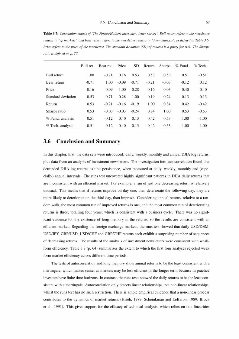
3.6. Conclusion and Summary 63
Table 3.7: Correlation matrix of ‘The Forbes/Hulbert investment letter survey’. Bull return refers to the newsletter
returns in ‘up markets’, and bear return refers to the newsletter returns in ‘down markets’, as defined in Table 3.6.
Price refers to the price of the newsletter. The standard deviation (SD) of returns is a proxy for risk. The Sharpe
ratio is defined on p. 77.
Bull ret. Bear ret. Price SD Return Sharpe % Fund. % Tech.
Bull return 1.00 -0.71 0.16 0.53 0.53 0.53 0.51 -0.51
Bear return -0.71 1.00 -0.09 -0.71 -0.21 -0.03 -0.12 0.12
Price 0.16 -0.09 1.00 0.28 -0.16 -0.03 0.40 -0.40
Standard deviation 0.53 -0.71 0.28 1.00 -0.19 -0.24 0.13 -0.13
Return 0.53 -0.21 -0.16 -0.19 1.00 0.84 0.42 -0.42
Sharpe ratio 0.53 -0.03 -0.03 -0.24 0.84 1.00 0.53 -0.53
% Fund. analysis 0.51 -0.12 0.40 0.13 0.42 0.53 1.00 -1.00
% Tech. analysis -0.51 0.12 -0.40 -0.13 -0.42 -0.53 -1.00 1.00
3.6 Conclusion and Summary
In this chapter, first, the data sets were introduced: daily, weekly, monthly and annual DJIA log returns,
plus data from an analysis of investment newsletters. The investigation into autocorrelation found that
detrended DJIA log returns exhibit persistence, when measured at daily, weekly, monthly and (espe-
cially) annual intervals. The runs test uncovered highly significant patterns in DJIA daily returns that
are inconsistent with an efficient market. For example, a run of just one decreasing return is relatively
unusual. This means that if returns improve on day one, then deteriorate the following day, they are
more likely to deteriorate on the third day, than improve. Considering annual returns, relative to a ran-
dom walk, the most common run of improved returns is one, and the most common run of deteriorating
returns is three, totalling four years, which is consistent with a business cycle. There was no signif-
icant evidence for the existence of long memory in the returns, so the results are consistent with an
efficient market. Regarding the foreign exchange markets, the runs test showed that daily USD/DEM,
USD/JPY, GBP/USD, USD/CHF and GBP/CHF returns each exhibit a surprising number of sequences
of decreasing returns. The results of the analysis of investment newsletters were consistent with weak-
form efficiency. Table 3.8 (p. 64) summarises the extent to which the first four analyses rejected weak
form market efficiency across different time periods.
The tests of autocorrelation and long memory show annual returns to be the least consistent with a
martingale, which makes sense, as markets may be less efficient in the longer term because in practice
investors have finite time horizons. In contrast, the runs tests showed the daily returns to be the least con-
sistent with a martingale. Autocorrelation only detects linear relationships, not non-linear relationships,
whilst the runs test has no such restriction. There is ample empirical evidence that a non-linear process
contributes to the dynamics of market returns (Hsieh, 1989; Scheinkman and LeBaron, 1989; Brock
et al., 1991). This gives support for the efficacy of technical analysis, which relies on non-linearities

64 Chapter 3. Characterization
Table 3.8: The extent to which the four statistical tests rejected weak form market efficiency across different time
periods.
Daily Weekly Monthly Annual
Autocorrelation inefficient inefficient
Runs test 1 inefficient
Runs test 2 inefficient inefficient
Long memory
being present Neftci (1991). In their review paper, Park and Irwin (2004) found that, on average, non-
linear methods outperformed genetic programming in all three types of market considered: stock mar-
kets, futures markets and currency markets. So are stock markets efficient or not? In sum, this chapter
reconciles the apparent efficiency of markets according to linear statistical tests with the potential for
non-linear forecasting methods to generate above-average risk-adjusted returns. Whilst the results of
the investment newsletter analysis implied that technical analysis, as applied by the newsletter writers,
holds no value. This is not surprising, as most such practitioners take a naive discretionary approach to
technical analysis.
The successful application of supervised learning relies upon domain knowledge (Wolpert, 1996).
The results of the second runs test—that uncovered surprising patterns in DJIA daily returns—are used
to construct an algorithm that forecasts the DJIA in Section 5.1.

65
Chapter 4
Modelling
The focus of this chapter—the second part of the time series trilogy—is modelling. The
experiments are chosen because they each allow us to model markets and investors’ risk
preferences using a realistic bottom-up empiricallly-valid approach, with a focus on sim-
plicity and realism. The primary aim is to build an agent-based artificial stock market and
explore the effect of the ratio of fundamental analysts to technical analysts, and to ascertain
whether and when the resultant time series displays the statistical properties exhibited by a
real market, i.e. reproduces the stylized facts described in Section 2.3.4. This experiment is
published as Sewell (2012c). Whilst Sewell (2011a) describes the evolution of the heuristics
and biases used in the artificial stock market, work that was removed from the thesis to save
space. The second experiment models investors’ risk preferences and develops a novel in-
vestment performance measurement metric, cumulative prospect theory certainty equivalent
(CPTCE). Sewell (2009b) relates to this experiment.
4.1 An Artificial Stock Market
4.1.1 Design
Multiagent Systems
A multiagent system is a system in which several interacting, autonomous, intelligent agents pursue some
set of goals or perform some set of tasks. A literature review was given on p. 44. Let’s consider some
valid criticisms of the approach. Agent-based modelling can stand accused of being poor science. To do
science, one needs ways to test hypotheses and reach general conclusions. Some of the problems with
multiagent systems:
• Too many free parameters.
• In common with all empirical research, one can always find evidence to support what one seeks to
prove. Too many possible explanations of the results leads to the opportunity for story telling.

66 Chapter 4. Modelling
• No general theoretical way to know whether a given simulation configuration is the only way to
get from some set of initial conditions to a result or one of a family of hundreds or millions of
ways to get to a result.
• Model validation can be complicated.
• Difficult to verify that the models are consistent enough to be useful.
Daniel Kahneman shared the Nobel Prize in Economics in 2002 with Vernon Smith. Economists once
thought of their science as inherently non-experimental, but Smith pioneered laboratory experimental
economics, and spearheaded ‘wind tunnel tests’, where trials of new markets could be tried out in the
lab before being implemented in the real world, giving policy makers a better understanding of how a
new market is likely to work in practice. Going one step further, from the laboratory to the computer,
on balance I consider agent-based modelling to be an effective way of studying behavioural finance,
because empirical results derived from the laboratory can be aggregated and modelled flexibly and at
low cost.
4.1.2 Implementation
The literature on behavioural finance was reviewed in Section 2.4.1 (p. 39). From my work on the
evolutionary foundations of heuristics and biases (Sewell, 2011a), I identified the following heuristics
and biases in the modern day investor/trader.
Overconfidence is likely to lead investors to trade too much, generally preferring actively managed
funds. Excess overconfidence among males in particular explains the popularity of trading among
men.
Optimism naturally creates a ‘bullish’ tendency and can create asymmetry in the behaviour of markets.
Availability could, for example, cause us to purchase shares in a company simply because it comes to
mind more readily.
Herding can lead investors to focus only on a subset of securities, whilst neglecting other securities
with near identical exogenous characteristics.
Representativeness leads analysts to believe that observed trends are likely to continue. Representative-
ness causes trend following by technical analysts and overreaction among fundamental analysts.
Anchoring is likely to cause fundamental analysts to underreact, for example to earnings announce-
ments.
Overconfidence leads to excess trading and helps create a liquid market in the first place, optimism
likely increases market participation in general, whilst availability and herding will generally only effect
a subset of stocks so their impact would be diluted when aggregated across stocks in general. So I only
implement the final two heuristics/biases above, which are the most relevant regarding market impact.

4.1. An Artificial Stock Market 67
In summary, following Barberis et al. (1998) we expect underreaction to news but an overreaction to a
series of good or bad news from fundamental analysts, and trend following from technical analysts. We
do not have sufficient news data to test this hypothesis directly, but would expect it to generate kurtosis
and non-linearities in market data, which are indeed found in real markets (Cont, 2001).
Theoretical Model of Market Action
Introduction
First, a reminder of three definitions.
Fundamental analysis A method of forecasting markets through the analysis of relevant news.
Technical analysis A method of forecasting markets through the analysis of data generated from the
activity of trading itself. This was covered in detail on pp. 41–44.
Multiagent system A system in which several interacting, autonomous, intelligent agents pursue some
set of goals or perform some set of tasks. See p. 44.
The objective is to model a stock market using a multiagent system. The implementation uses Mi-
crosoft Excel as the price may be modelled as a function of aggregate supply and aggregate demand.
The main criteria is to be as realistic as possible; that is, the problem domain is mapped onto the model.
The only other criteria is to keep the model as simple as possible (which is often at odds with the quest
for realism). In practice, traders are essentially divided into two groups, fundamental analysts (who tend
to be longer term) and technical analysts (who tend to be shorter term); the distribution of agents in our
model shall mirror this dichotomy (Lux (1995) and Hong and Stein (1999) took a similar approach).
Reviewing the existing literature, at one extreme, some artificial markets employ agents with zero intel-
ligence (Gode and Sunder, 1993; Farmer et al., 2005). Whilst in some implementations agents are able
to swap between technical analysis and fundamental analysis depending on their profits (they have the
ability to learn) (Lux, 1998; Lux and Marchesi, 1999, 2000). I reject the application of zero intelligence
agents, as in practice most traders have a reasonably consistent strategy (which may or may not work).
I also reject the idea of agents swapping between technical analysis and fundamental analysis, because
in practice technical analysts and fundamental analysts tend to be somewhat antagonistic towards each
other.1 Finally, I reject the notion of agents learning. Due to a combination of overconfidence, a lim-
ited exposure to markets (at most one working life) and noise, real traders do not learn how to predict
markets2 (even if they did, as new traders replaced the old, they would not improve ‘on average’); this
stasis is trivially mirrored. Indeed, Martinez-Jaramillo (2007) and Martinez-Jaramillo and Tsang (2009)
developed an artificial financial market and investigated the effects on the market when the agents learn,
and, on average, their model without learning replicated the stylized facts most accurately (though not by
much). In my model the technical analysts simply follow the technician’s number one rule: they follow
1‘Fundamental analysts have referred to Technical analysts as indulging in voodoo and shamanism and a technician once
described the former’s efforts as “fundamentally a waste of time”’ (Society of Technical Analysts, 1999, p. 2).2Indeed, there is a negative relationship between the tenure of a hedge fund manager and hedge fund returns (Boyson, 2003).

68 Chapter 4. Modelling
the trend, so the model fails to replicate some of the more complex strategies that chartists follow. The
artificial market operates such that each time step represents one trading day, and the stock price may be
interpreted as a daily closing price.
Below is a taxonomy of five groups of market participants, including three types of fundamental
analyst and two types of technical analyst. Note that technical analysis is a behavioural bias (representa-
tiveness), here a ‘good’ technical analyst is one who accurately and consistently trades according to the
rules of technical analysis.
Fundamental analysts
Poor Trade randomly—fundamental analysts lacking sufficient skills or experience to analyse a
company will make mistakes at random.
Real Consistent, correlated and irrational—Homo sapiens employed as fundamental analysts will
be susceptible to behavioural biases and make systematic errors.
Good Rational—Skilled fundamental analysts (Homo economicus) with the ability to accurately
analyse a company, and thus evaluate the value of its stock.
Technical analysts
Poor Trade randomly—those employed as technical analysts but lacking the ability or experience
to follow the rules of technical analysis.
Good Consistent, correlated and irrational—experienced technical analysts able to trade in accor-
dance with the rules of technical analysis.
Assuming that all five types of market participant exist (they do), with imperfect arbitrage opportunities
and no 100 per cent rational traders, the resultant effect on the market is the aggregate effect of real
fundamental analysts trading against good technical analysts. A multiagent system with technical and
fundamental agents is used to model price action. This work employs a bottom-up approach and has
been developed from first principles.
Fundamental Analysis
News, by definition, is unpredictable (otherwise it would have been reported yesterday), so let us assume
that the cumulative impact of relevant news on a stock follows a geometric random walk. Fundamental
analysts calculate the intrinsic value of a stock by the analysis of relevant news. Let the exogenous
variable Vt be the perceived fundamental value at time t, where log V follows a random walk. Note that
V is a latent variable, it is not directly observable, but changes in the variable are observable in the form
of news, and the model assumes that V may be calculated. If V increases, this corresponds to good
news, if it decreases, this corresponds to bad news. The fundamental analysts trade on the basis of this
perceived fundamental value alone (they do not consider historical prices). At each time step, if the price
of a stock is below (above) the perceived fundamental value of the stock, fundamental analysts will take
a long (short) position in proportion to the logarithm of the perceived fundamental value over the price.

4.1. An Artificial Stock Market 69
In other words, the fundamental analysts trade in such a way that they always move the price towards
the fundamental value. Formally,
logVtVt−1
> 0 represents good news, and
logVtVt−1
< 0 represents bad news.
Let nf be the proportion of the total number of trades made by fundamental analysts and Pt the price at
time t. The idea is to model an underreaction to news, but an overreaction to a series of good or bad news.
Therefore, the fundamental agents overreact to three or more successive good (or bad) news items, are
neutral towards exactly two successive good (or bad) news items and underreact otherwise. In a market
populated entirely by fundamental analysts, the log return of the price between time t and time t + 1
would be Ft. The values for the reaction variable, r, below, are chosen with reference to Theobald and
Yallup (2004)’s direct measures of the degrees of overreaction and underreaction in financial markets
(speeds of adjustment of asset prices towards their intrinsic values), but the figures used here are subject
to significant uncertainty.
Ft = r logVtPt
(4.1.1)
where
r =
1.1 if Vt > Vt−1 > Vt−2 > Vt−3 or
Vt < Vt−1 < Vt−2 < Vt−3; else
1 if Vt > Vt−1 > Vt−2 or Vt < Vt−1 < Vt−2;
else
0.9.
(4.1.2)
Technical Analysis
The second class of ‘actors’ employed in the model are technical analysts.
A Note on Terminology
When referring to technical analysis, the noun chartist and related verb charting are also used, sometimes
referring to a subset of technical analysis. Also, technical analysts are often referred to as ‘noise traders’
in the academic literature (‘noise’ being anything other than news).
Definition
Let us define technical analysis. Formally, if P is price, D is data generated by the process of trading, t
is time, E is expectation and | the Bayesian probability conditioning bar, then technical analysis is the
art of inferring E(Pt|t>0|Dt|t<0). In other words, the forecasting of future market prices by means of
analysis of historical data generated by the process of trading.

70 Chapter 4. Modelling
Taxonomy
A taxonomy of the various methods of technical analysis applied by practitioners is given in Appendix H
(pp. 171–172). Of the 26 techniques listed, according to the academic literature there is evidence for the
efficacy of about 11, but no evidence for the efficacy of the remaining 15.
Assumptions
Technical analysts rely on the assumption that markets discount everything except information generated
by market action, ergo, all you need is data generated by market action.
Why is Technical Analysis so Popular?
The artificial stock market developed assumes that technical analysts exist, and they are afforded the
same prominence as fundamental analysts. This is a realistic assumption, because despite the fact that
technical analysis holds little value, technical analysts do indeed exist in significant numbers. If the
weak form of the efficient market hypothesis holds, then technical analysis has no value. Conversely, for
technical analysis to work requires that the weak (and therefore the semi-strong and strong) forms of the
EMH are false. Also, if a market price follows a Markov process then technical analysis applied to the
price holds no value. Why, then, is technical analysis so popular? People often predict future uncertain
events by taking a short history of data and asking what broader picture this history is representative of
(independent of other information about its actual likelihood). This is a heuristic known as representa-
tiveness (Tversky and Kahneman, 1974). Technical analysis is representativeness. Below are some more
psychological explanations of why a large number of people have a strong belief in technical analysis.
Communal reinforcement Communal reinforcement is a social construction in which a strong belief
is formed when a claim is repeatedly asserted by members of a community, rather than due to the
existence of empirical evidence for the validity of the claim.
Selective thinking Selective thinking is the process by which one focuses on favourable evidence in
order to justify a belief, ignoring unfavourable evidence.
Confirmation bias Confirmation bias is a cognitive bias whereby one tends to notice and look for infor-
mation that confirms one’s existing beliefs, whilst ignoring anything that contradicts those beliefs.
It is a type of selective thinking.
Self-deception Self-deception is the process of misleading ourselves to accept as true or valid what we
believe to be false or invalid by ignoring evidence of the contrary position.
The technician’s number one rule is that they follow the trend. Quoting a best-selling practitioner’s
book on technical analysis (Murphy, 1999, p. 49), ‘The concept of trend is absolutely essential to the
technical approach to market analysis. All of the tools used by the chartist—support and resistance
levels, price patterns, moving averages, trendlines, etc.—have the sole purpose of helping to measure the
trend of the market for the purpose of participating in the trend. We often hear such familiar expressions

4.1. An Artificial Stock Market 71
as “always trade in the direction of the trend,” never buck the trend,” or “the trend is your friend.”’ So, in
this model, technical analysts follow the trend, i.e. display momentum; they consider the historical price
of a stock, and nothing else. At each time step, they exhibit persistence by trading in such a way that
the price is biased towards continuing in the same direction as the recent past. Let nt be the proportion
of trades made by technical analysts. The technical analysts’ trend-following strategy looks back three
days and weights the price changes by recency. In this model if the market were populated entirely by
technical analysts, the log return of the price between time t and time t+ 1 would be Tt.
Tt = c3 logPt−2
Pt−3+ c2 log
Pt−1
Pt−2+ c log
PtPt−1
, (4.1.3)
where the coefficients c3, c2 and c form an increasing geometric sequence so that more recent price
changes have a greater impact on T , and sum to one. Solving c3 + c2 + c = 1, which has one real root,
gives us c = 0.544.
Stock Price Returns
To summarise:
V is a latent variable and follows a lognormal random walk,
F is the effective log return generated by fundamental analysts, and is a function of V and P ,
T is the effective log return generated by technical analysts, and is a function of P , and
P is price, and is a function of F and T .
In the final generative model, changes in price are determined by the following equation:
logPt+1
Pt= nfFt + ntTt. (4.1.4)
By way of example, if Pt > Vt, the fundamental analyst believes that the stock is overvalued.
Those who hold the stock may sell it, those who don’t may either do nothing or short the stock. Or the
fundamental analyst may publish a recommendation that the stock is a sell. The point is that on aggregate
the actions of the fundamental analysts will put pressure on the stock price to fall. If, however, the
technical analysts put even greater selling pressure on the stock, the fundamental analysts will become
net buyers.
Taylor (2005) includes various statistics on stocks, repeated in Table 4.1 (p. 72). In order to deter-
mine the mean and standard deviation of the Gaussian random variable log VtVt−1
, first, a realistic ratio of
50% fundamental trades and 50% technical trades (nf = 0.5 and nt = 0.5) was chosen. Then the mean
and standard deviation space was discretised, an exhaustive enumeration of return sequences generated,
one for each discrete parameter setting pair, and the pair for which the mean and standard deviation of
the simulated stock returns most closely matched those of the empirical data in Table 4.1 was chosen.
This resulted in a mean of 0.0013 and a standard deviation of 0.023 for the Gaussian random variable
log VtVt−1
. The model was run over 50,000 days twenty times, and averages of various statistics calculated.

72 Chapter 4. Modelling
Table 4.1: Statistics of daily stock log returns (Taylor, 2005)
Coca Cola General Electric General Motors Glaxo Marks & Spencer Shell Mean Standard deviation
Mean 0.001167 0.000742 0.000558 0.001473 0.000725 0.000763 0.000905 0.000344
Standard deviation 0.0169 0.0151 0.0176 0.0179 0.0166 0.0130 0.0162 0.0018
Skewness 0.08 0.03 0.13 0.33 0.03 0.23 0.14 0.12
Kurtosis 5.68 5.43 4.56 6.93 4.40 5.18 5.36 0.91
Returns autocorrelation -0.035 -0.023 -0.003 0.08 0.034 0.045 0.016 0.044
Absolute returns autocorrelation 0.329 0.224 0.204 0.247 0.155 0.196 0.226 0.059
Squared returns autocorrelation 0.545 0.303 0.398 0.414 0.288 0.293 0.374 0.100
4.1.3 Testing
Recall that Pt is the price of a stock at time t, and Vt is the perceived fundamental value of the stock at
time t. Note that Shiller (1981) calculated that stock market volatility is five to thirteen times too high
to be attributed to new information, so we should not expect the standard deviation of P log returns to
equal the standard deviation of V log returns (although perhaps surprisingly, in this model, the latter
is slightly greater). Table 4.2 (p. 73) lists various statistics of the returns generated by the model as
the proportion of technical analysts to fundamental analysts varies. Figure 4.1 (p. 73) shows the mean
return per analyst, as the proportion technical analysts/fundamental analysts varies. Figure 4.2 (p. 74)
shows the mean Sharpe ratio (assuming a risk-free interest rate of 0%) of the analysts, as the proportion
technical analysts/fundamental analysts varies. Figure 4.3 (p. 74) shows the mean, standard deviation
and skewness of market log returns as the proportion technical analysts/fundamental analysts varies.
Figure 4.4 (p. 75) shows the kurtosis of market log returns as the proportion technical analysts/funda-
mental analysts varies. Figure 4.5 (p. 75) shows the autocorrelations of returns, absolute returns and
squared returns as the proportion technical analysts/fundamental analysts varies. Table 4.3 (p. 76) shows
that with a realistic proportion of technical and fundamental trades, the artificial stock market replicates
mean returns, the standard deviation of returns, the absolute returns correlation and the squared returns
correlation of a real stock market. However, the artificial stock market failed to accurately replicate the
skewness, kurtosis and autocorrelation of returns.
Conclusion
Results showed that whether a fundamental analyst, or a technical analyst, it pays to be among the
majority. Mean stock returns are low and positive regardless of the relative proportions of analysts, this
is consistent with a real market.
As the number of technical analysts increases, the standard deviation of returns decreases, whilst
remaining realistic, whilst the skewness increases. The model exhibited slight negative skewness, whilst
real markets exhibit significant positive skewness. Whilst the kurtosis of market returns peaks at around
0.25 with around 40 per cent technical analysts, and rapidly declines as the number of technical analysts
exceeds 90 per cent. In contrast, the kurtosis of daily stock returns in real markets is around 5.
The autocorrelation of returns is close to zero with 100 per cent fundamental analysts, and ap-

4.1. An Artificial Stock Market 73
Table 4.2: Statistics generated by the artificial stock market
Fundamental analysts (%) 100 90 80 70 60 50 40 30 20 10 0
Technical analysts (%) 0 10 20 30 40 50 60 70 80 90 100
Mean fundamental analyst return 0.0011 0.0012 0.0012 0.0015 0.0017 0.0000 -0.0026 -0.0033 -0.0053 -0.0103
Mean technical analyst return -0.0107 -0.0049 -0.0034 -0.0026 0.0000 0.0017 0.0014 0.0013 0.0011 0.0010
Mean fundamental analyst Sharpe ratio 0.0461 0.0514 0.0535 0.0576 0.0601 0.0001 -0.0653 -0.0710 -0.0743 -0.0752
Mean technical analyst Sharpe ratio -0.0514 -0.0535 -0.0576 -0.0601 -0.0001 0.0653 0.0710 0.0743 0.0752
Mean return 0.0011 0.0011 0.0010 0.0010 0.0010 0.0010 0.0010 0.0010 0.0011 0.0010 0.0010
Returns standard deviation 0.0226 0.0208 0.0194 0.0182 0.0172 0.0163 0.0155 0.0149 0.0143 0.0138 0.0108
Returns skewness -0.0552 -0.0533 -0.0503 -0.0434 -0.0348 -0.0393 -0.0201 -0.0136 -0.0178 -0.0043 0.0025
Returns kurtosis 0.0822 0.1512 0.2010 0.2350 0.2476 0.2371 0.2073 0.1348 0.1100 0.0394 -1.4268
Returns autocorrelation 0.0658 0.2038 0.3338 0.4566 0.5690 0.6710 0.7627 0.8423 0.9088 0.9617 1.0000
Absolute returns autocorrelation 0.0093 0.0364 0.0931 0.1750 0.2803 0.4045 0.5403 0.6730 0.7984 0.9083 1.0000
Squared returns autocorrelation 0.0088 0.0401 0.1029 0.1899 0.3021 0.4259 0.5650 0.6974 0.8226 0.9244 1.0000
-0.012
-0.01
-0.008
-0.006
-0.004
-0.002
0
0.002
0.004
0 20 40 60 80 100
Fundamental analysts
Technical analysts
Figure 4.1: Mean log return (P&L) per analyst, as the proportion technical analysts/fundamental analysts varies.
Both technical analysts and fundamental analysts profit if and only if they are in the majority. In both cases, the
most profitable position to be in is a majority of around 60% and the greatest losses occur when in a small minority.

74 Chapter 4. Modelling
-0.1
-0.08
-0.06
-0.04
-0.02
0
0.02
0.04
0.06
0.08
0.1
0 20 40 60 80 100
Technical analysts (%)
Fundamental analysts
Technical analysts
Figure 4.2: Mean Sharpe ratio per analyst, as the proportion technical analysts/fundamental analysts varies. Both
technical analysts and fundamental analysts have a positive Sharpe ratio if and only if they are in the majority. In
both cases, it pays to be in a majority of over 60%.
-0.06
-0.05
-0.04
-0.03
-0.02
-0.01
0
0.01
0.02
0.03
0 20 40 60 80 100 Mean
Standard deviation
Skewness
Figure 4.3: Mean, standard deviation and skewness of market log returns as the proportion technical analysts/-
fundamental analysts varies. Mean log returns are necessarily constant, low and positive. Volatility (standard
deviation) gradually declines as the number of technical analysts increses. Skewness is almost always negative, and
increases as the proportion of technical analysts increases, approaching zero as the proportion of technical analysts
approaches 100%. The mean log returns are consistent with those of a real market, the standard deviation in the
region of 40–70% technical analysts is realistic, whilst the negative skewness is inconsistent with a real market.

4.1. An Artificial Stock Market 75
-1.6
-1.4
-1.2
-1
-0.8
-0.6
-0.4
-0.2
0
0.2
0.4
0 20 40 60 80 100
Kurtosis
Figure 4.4: Kurtosis of market log returns as the proportion technical analysts/fundamental analysts varies. The
kurtosis is low but positive with 0–90% technical analysts, but crosses zero with 90% technical analysts and declines
rapidly as the proportion of technical analysts approaches 100%. The kurtosis is significantly lower than that
exhibited by a real market.
0
0.1
0.2
0.3
0.4
0.5
0.6
0.7
0.8
0.9
1
0 20 40 60 80 100
Technical analysts (%)
Absolute returns
Squared returns
Figure 4.5: Autocorrelations of market log returns, absolute log returns and squared log returns as the proportion
technical analysts/fundamental analysts varies. All three autocorrelations are positive and rise as the proportion
of technical analysts approaches 100%. The autocorrelation in a real market is much closer to zero, whilst the
absolute returns autocorrelation with 30–40% technical analysts and the squared returns autocorrelation for 40–
50% technical analysts are both realistic.

76 Chapter 4. Modelling
Table 4.3: Range of proportions of technical analysts in the artificial stock market that replicate stylized facts.
Overall, the artificial stock market is most realistic with 40–50% technical analysts, which may well be consistent
with a real market.
Statistic Proportion of technical analysts
Mean return 0–100%
Returns standard deviation 40–70%
Returns skewness none
Returns kurtosis none
Returns autocorrelation none
Absolute returns autocorrelation 30–40%
Squared returns autocorrelation 40–50%
proaches one as the proportion of technical analysts approaches 100 per cent. Unsurprisingly, the trend-
following technical analysts created positive autocorrelations in returns in the model, but autocorrela-
tions of returns are close to zero in real markets. The autocorrelation of absolute and squared returns
is realistic only around the region of 30%–50% technical analysts. How has the model fared in light of
the criticisms of multiagent systems that were highlighted in Section 4.1.1 (p. 65)? The main concern,
that one can vary any free parameter until one obtains the result that one desires, i.e. high kurtosis, was
mitigated by keeping the number of varying parameters to a minimum, by using realistic assumptions.
Martinez-Jaramillo (2007) and Martinez-Jaramillo and Tsang (2009) investigated the different condi-
tions under which the statistical properties of an artificial stock market resemble those of a real financial
market. Their approach replicated the stylized facts of a financial market far more accurately than my
own; this was possible by including and adjusting a much larger number of parameters.
4.2 Investment Performance Measurement
4.2.1 Design
A brief literature review on investment performance measurement was given in Section 2.4.5 (p. 46).
In this section, the Sharpe ratio, Sortino ratio and Omega are improved upon by developing a new
performance metric, cumulative prospect theory certainty equivalent (CPTCE).
A 4 per cent return on a savings account will always be preferable to a 3 per cent return. The choice
is not as clear cut when there is an element of risk. If you are offered a gamble, what would be a fair
value for you to pay (or be paid) for the opportunity to take it? Consider a 50 per cent chance of losing
£100 and a 50 per cent chance of winning £100. The expected return is £0. But what about risk? There
is no principled way of measuring risk.3
3For an overview of the philosophy of risk, see Sewell (2012e).

4.2. Investment Performance Measurement 77
Kelly (1956) and Breiman (1961) showed that in order to achieve maximum growth of wealth,
one should maximize the expected value of the logarithm of wealth after each period. However, most
investors are unwilling to endure the volatility of wealth that such a strategy entails, and as John Maynard
Keynes reminded us, in the long run, we’re all dead. For this reason, various risk-adjusted performance
metrics have been developed. Any risk-adjusted measure of performance makes assumptions about
investors’ risk preferences. It is my contention that one could measure risk-adjusted performance in
terms of the way people actually behave. Empirical research tells us that, in practice, people care about
losses and gains rather than absolute wealth, evaluate probabilities incorrectly, are loss averse, risk averse
for gains, risk seeking for losses and have non-linear preferences.
The Sharpe ratio is the most popular investment performance metric. Where R is the asset return,
Rf is the return on a benchmark asset, such as the risk free rate of return,E[R−Rf ] is the expected value
of the excess of the asset return over the benchmark return, and σ =√V ar[R−Rf ] is the standard
deviation of the excess return,
Sharpe ratio =E[R−Rf ]
σ. (4.2.1)
The Sharpe ratio makes implicit assumptions which stem from the capital asset pricing model
(CAPM) (Treynor, 1962; Sharpe, 1964; Lintner, 1965; Mossin, 1966)4: it assumes either 1) normally
distributed returns or 2) mean-variance preferences.
Both assumptions are suspect:
1. The returns generated by most hedge funds exhibit negative skewness (Kat and Lu, 2002).
2. In addition to the mean and variance, people also care about skewness (they like it positive) and
kurtosis (they don’t like it), and higher moments matter too (Scott and Horvath, 1980).
Because the Sharpe ratio is oblivious of all moments higher than the variance, it is prone to manipulation
by strategies that can change the shape of the probability distribution of returns. Mathematically, max-
imizing the Sharpe ratio is a standard quadratic programming optimization problem with the constraint
that the mean excess return is fixed. Goetzmann et al. (2002) proved that the solution produces a reversed
lognormal distribution with a truncated right tail and a fat left tail leading to extreme negative skewness,
as shown in Figure 4.6 (p. 78. The optimal strategy involves selling out-of-the-money calls (to remove
the right tail of the distribution) and selling out-of-the-money puts (to enhance the left tail) in an uneven
ratio. Such a strategy would generate a regular return from writing options, but would have a large ex-
posure to extreme negative events. In other words, a manager with no special information can improve
his Sharpe ratio in such a way that the distribution of returns exhibits negative skewness. As mentioned
above, most investors prefer positive skewness, therefore, although a high Sharpe ratio is good thing, a
high Sharpe ratio strategy is a bad thing.
4Under CAPM, the portfolio on the efficient frontier with the highest Sharpe ratio is the market portfolio. The slope of the
capital market line equals the market (i.e. index) Sharpe ratio.

78 Chapter 4. Modelling
Figure 4.6: Maximal Sharpe ratio (Goetzmann et al., 2002)
4.2.2 Implementation
Cumulative prospect theory certainty equivalent
When presented with an uncertain payoff, the certainty equivalent is the guaranteed payoff at which
a person is indifferent between accepting the uncertain payoff and the guaranteed payoff. Certainty
equivalent varies according to individuals’ risk preferences, and for a risk averse individual the certainty
equivalent will be less than the expected value of the gamble. An attractive property of certainty equiv-
alent is that so long as risk preferences are known, it reduces a probability distribution to a single value.
This has obvious advantages for an investor who wishes to compare distributions of returns.
A new investment performance measurement algorithm is developed, which is an implementation
of Tversky and Kahneman’s cumulative prospect theory (Tversky and Kahneman, 1992) (explained on
p. 45). The measure is known as cumulative prospect theory certainty equivalent (or CPTCE). This
measure tells us that, on average, people would wish to be paid £22.30 to take the gamble offered on
p. 76. The equations used to derive this figure follow.
The two weighting functions, w+ for gain-ranked probabilities andw− for loss-ranked probabilities
are defined as follows:
w+(p) =pγ
(pγ + (1− p)γ)1γ
(4.2.2)
w−(p) =pδ
(pδ + (1− p)δ) 1δ
(4.2.3)

4.2. Investment Performance Measurement 79
γ and δ are parameters that Tversky and Kahneman determined empirically as γ = 0.61 and δ = 0.69.
The value (utility) function (taken from Kobberling (2002)) has a loss aversion parameter λ, and is
as follows:
U(x) =
f(x) if x > 0
0 if x = 0
λg(x) if x < 0
(4.2.4)
where f(x) and g(x) are defined as follows:
f(x) =
xα if α > 0
log(x) if α = 0
1− (1 + x)α if α < 0
(4.2.5)
g(x) =
−(−x)β if β > 0
− log(−x) if β = 0
(1− x)β − 1 if β < 0
(4.2.6)
Again, the parameters α, β and λ were determined by Tversky and Kahneman empirically, α = 0.88,
β = 0.88 and λ = 2.25.
Wakker (2010)’s step-by-step description of the procedure for calculating the PT (prospect theory)
value of a prospect follows. Note that steps 1 and 2 together determine the complete sign-ranking, and
losses (steps 6–8) are treated symmetrically to gains (steps 3–5).
1. Completely rank outcomes from best to worst.
2. Determine which outcomes are positive and which are negative.
3. For each positive outcome, calculate the gain-rank g.
4. For all resulting gain-ranks, calculate their w+ value.
5. For each positive outcome a, calculate the marginal w+ contribution of its outcome probability p
to its rank; i.e. calculate5 w+(p+ g)− w+(g).
6. For each negative outcome, calculate the loss-rank `.
7. For all resulting loss-ranks, calculate their w− value.
8. For each negative outcome b, calculate the marginal w− contribution of its probability q to its
loss-rank; i.e., calculate6 w−(q + `)− w−(`).
9. Determine the utility of each outcome, U(x).
10. Multiply the utility of each outcome by its decision weight.
5p+ g is the gain-rank of the gain in the prospect ranked worse than but next to a considered in step 3.6q + ` is the loss-rank of the loss in the prospect ranked better than but next to b considered in step 6.

80 Chapter 4. Modelling
11. PT value is the sum of the results of step 10.
12. Certainty equivalent is then a function of PT value, α, β and λ, as described in the code in Ap-
pendix I (pp. 173–182).
Cumulative prospect theory certainty equivalent makes up part of a more general performance mea-
surement calculator which I wrote in PHP for the Web and in Visual Basic for Excel, both of which are
freely available online.7 It calculates mean return, standard deviation, skewness, kurtosis, beta, Jensen’s
alpha, Sharpe ratio, Sortino ratio, Treynor’s measure, information ratio, Stutzer ratio, Omega, M2, T2
and maximum drawdown. To avoid ambiguity, the source code for CPTCE is included in Appendix I
(pp. 173–182). Note that Kahneman and Tversky’s prospect theory is concerned with absolute gains and
losses, whilst here the concept is mapped onto returns (because, in terms of assessing the performance
of an investment, that is what an investor is interested in).
4.2.3 Testing
A Monte Carlo simulation was used to simulate 20,000 funds, each with 15 daily returns, r. Each fund
allocated a randomly-chosen proportion (between 0% and 100%), p, of their assets to a risky asset, and
put the rest in a risk-free asset. The risk-free rate, f , and the threshold used for the Sortino ratio, Omega
and the upside potential ratio are both set to 3% (0.012% per day), the mean return for the risky asset, µ,
0.0905% per day and the risky asset standard deviation, σ, 1.62% per day (averages taken from Taylor
(2005) and repeated in Table 4.1 (p. 72)). The probability used by Conditional VaR and Modified VaR
was set to 0.05. The model is defined as follows.
r = (1− p)f + pN (µ, σ2)
Results are given in Table 4.4 (p. 81). The table shows the correlations between the Sharpe ratio
and CPTCE versus various statistics and performance metrics. The statistics show that CPTCE is more
risk averse than the Sharpe ratio, penalizing both the proportion of funds allocated to a risky asset and
the standard deviation of returns to a greater degree. Significantly, the Sharpe ratio is indifferent towards
skewness, but CPTCE rewards positive skewness, and the latter is more consistent with investors’ risk
preferences (Scott and Horvath, 1980). Further, CPTCE punishes maximum drawdown to a greater
extent than the Sharpe ratio, which is also more consistent with many investor’s utility. This experiment
was conducted using a Performance Metric Analysis Excel spreadsheet I wrote in Visual Basic, which
is freely available online.8 A reasonable criticism of CPTCE is that prospect theory is descriptive, and
one could argue that an investment manager is responsible for implementing an algorithm that employs
sensible prescriptive risk preferences, as I argue in Sewell (2009b).
7http://www.performance-measurement.org8Ibid.

4.3. Conclusion and Summary 81
Table 4.4: The correlations between the Sharpe ratio and various statistics, and CPTCE and various statistics
Statistic Sharpe ratio CPTCE
Proportion in risky asset 0.01 -0.48
Arithmetic mean 0.84 0.76
Standard deviation 0.00 -0.53
Skewness 0.01 0.15
Kurtosis 0.01 0.04
Sharpe ratio 1.00 0.70
Sortino ratio 0.80 0.61
Omega 0.65 0.50
CPTCE 0.70 1.00
Maximum drawdown -0.49 -0.87
Upside potential ratio 0.75 0.59
Calmar ratio 0.09 0.09
Conditional VaR 0.18 0.43
Modified VaR 0.14 0.15
4.3 Conclusion and Summary
Those heuristics and biases which contribute to behavioural finance were identified, and used to build
a theoretical model of market action which simulates the aggregates of many interacting agents. The
artificial stock market exposed the effect of varying the proportion of technical analysts to fundamental
analysts. The artificial market replicates mean returns, the standard deviation of returns, the absolute
returns correlation and the squared returns correlation of a real stock market, but failed to accurately
replicate the skewness, kurtosis and autocorrelation of returns. This implies that the model has failed to
capture some of the dynamics underlying the process of price formation, possibly due to being overly
simplistic. Finally, a contribution was made to investment performance measurement in the form of a
new metric, CPTCE, which is based on prospect theory. From a descriptive perspective, the risk metric
should be superior to any existing methods of performance measurement, as it accurately incorporates
people’s risk profiles.

82 Chapter 4. Modelling

83
Chapter 5
Forecasting
The goals of the experiments on forecasting are to 1) improve standard algorithms, and
2) beat the ‘state of the art’. The first piece of work concerns forecasting DJIA daily re-
turns. For the second set of work, for both theoretical and empirical reasons I opted to
use kernel methods for forecasting, and the class of algorithms are dealt with in general by
defining the kernel of a function, explaining the kernel trick and listing its advantages. The
section on design introduces the well-established example of a kernel method, the support
vector machine. It goes on to cover preprocessing data, model selection, feature selection
and software–I ported two implementations of SVMs to Windows and also added semi-
automated parameter selection. Finally, the Fisher kernel is covered. The section on imple-
mentation describes the foreign exchange data set, then details the five implementations of
kernel methods employed—a support vector machine, a Fisher kernel, the DC algorithm,
a Bayes point machine and a DC algorithm–Fisher kernel hybrid. The section on testing
includes results and a conclusion. The chapter is published as Sewell and Shawe-Taylor
(2012), though the results differ as the published article didn’t use a moving window for
training. In addition, Yan et al. (2008) provides a head-to-head evaluation of GP and SVM
forecasting, similar to the work in this chapter, and draws the same conclusion.
5.1 Forecasting DJIA Daily Returns
In Section 2.5.1 (p. 47) we saw that the key to developing successful machine learning algorithms is to
carefully consider the assumptions being made, which requires extracting as much domain knowledge as
possible. Chapter 3, on the characterisation of financial time series, included two runs tests, the second
of which uncovered surprising patterns in DJIA daily returns (Section 3.3.2).
This section uses those results to construct an algorithm that forecasts the DJIA. Although the DJIA
cannot be traded directly, there are investment products available that match the performance of the
DJIA, for example the SPDR Dow Jones Industrial Average ETF. First, recall the results of the second
runs test shown in Appendix E, and that an increasing run refers to a sequence of increasing returns such

84 Chapter 5. Forecasting
as -0.2, -0.1, 0, 0.1, 0.2, whilst a decreasing run refers to a sequence of decreasing returns such as 0.2,
0.1, 0, -0.1, -0.2. When compared to a random walk, returns were significantly less likely to increase or
decrease for just one day, and far more likely to deteriorate for 2–5 days in a row. As 97.2% of runs are
of length 3 or less and 99.5% of runs are of length 4 or less, we are mainly concerned with short runs.
This suggests a very simple trading algorithm: if the current return is greater than the previous return, go
long, else go short. Formally, if Pt is the closing price of the DJIA on day t,
if logPtPt−1
− logPt−1
Pt−2> 0 go long, else go short.
As in the chapter on characterisation, the data used to create the algorithm were the DJIA daily
closing prices from 1 October 1928 to 23 March 2012 downloaded from Yahoo! Finance. To test the
algorithm with out of sample data, DJIA daily closing prices from 26 March 2012 to 31 December 2015
were downloaded from the same source. Figure 5.1 shows the equity curve for the DJIA and the trading
system (no transaction costs have been deducted), and includes both the training set and the test set. It
-4
-2
0
2
4
6
8
10
12
14
16
19
25
19
30
19
35
19
40
19
45
19
50
19
55
19
60
19
65
19
70
19
75
19
80
19
85
19
90
19
95
20
00
20
05
20
10
20
15
Cu
mu
lati
ve lo
g re
turn
Year
Market Equity
Figure 5.1: Equity curves for the DJIA and the trading system
can be seen that, although the algorithm was created in sample, given its simplicity and the size of the
data set, significant overfitting of noise seems unlikely, so the equity curve is surprisingly impressive up
until 2002, when the dynamics of the market must have changed. However, the algorithm clearly fails to
outperform the market in the out of sample period (26 March 2012 onwards).
5.2 Kernel Methods
The motivation for using kernel methods (both theoretical and empirical) was given on p. 21. Below we
give a more formal treatment. The kernel trick is explained, and its advantages given.

5.3. Design 85
Kernel Trick
The kernel trick, first published by Aizerman et al. (1964), uses the kernel as a similarity measure.
Mercer’s theorem states that any continuous, symmetric, positive semi-definite kernel function K(x, y)
can be expressed as a dot product in a high-dimensional space.
If the arguments to the kernel are in a measurable space X , and if the kernel is positive semi-
definite—i.e.n∑i=1
n∑j=1
K(xi, xj)cicj ≥ 0
for any finite subset {x1, . . . , xn} of X and subset {c1, . . . , cn} (real-valued coefficients)—then there
exists a function ϕ(x) whose range is in an inner product space of possibly high dimension, V , such that
K(x, y) = 〈ϕ(x), ϕ(y)〉V .
Advantages
• The kernel defines a similarity measure between two data points and thus allows one to incorporate
prior knowledge of the problem domain.
• Most importantly, the kernel contains all of the information about the relative positions of the
inputs in the feature space and the actual learning algorithm is based only on the kernel function
and can thus be carried out without explicit use of the feature space. The training data only enter
the algorithm through their entries in the kernel matrix (a Gram matrix, see Appendix J.1 (p. 183)),
and never through their individual attributes. Because one never explicitly has to evaluate the
feature map in the high dimensional feature space, the kernel function represents a computational
shortcut.
• The number of operations required is not, in general, proportional to the number of features.
5.3 Design
This section introduces the well-established example of a kernel method, the support vector machine,
which is used as a benchmark algorithm. It goes on to cover the major issues that we must consider when
forecasting—preprocessing the data, model selection (which model to use), feature selection (which
inputs to use) and software. Finally, the Fisher kernel is covered, as an implementation is used for one
of the experiments.
Support Vector Machines
A support vector machine (SVM) is a supervised learning technique from the field of machine learn-
ing applicable to both classification and regression. Rooted in the statistical learning theory developed

86 Chapter 5. Forecasting
by Vladimir Vapnik and co-workers, SVMs are based on the principle of structural risk minimization
(Vapnik and Chervonenkis, 1974).
The background mathematics required includes probability, linear algebra and functional analysis.
More specifically: vector spaces, inner product spaces, Hilbert spaces (defined in Appendix J.2 (p. 183)),
operators, eigenvalues and eigenvectors. A good book for learning the background maths is Introductory
Real Analysis (Kolmogorov and Fomin, 1975).
Support vector machines (reviewed briefly on p. 49) are the most established example of kernel
methods. The literature on the application of SVMs to the financial domain was covered on pp. 49–52.
The basic idea of an SVM is as follows:
1. Non-linearly map the input space into a very high dimensional feature space (the ‘kernel trick’).
2. • In the case of classification, construct an optimal separating hyperplane in this space (a max-
imal margin classifier); or
• in the case of regression, perform linear regression in this space, but without penalising small
errors.
Preprocessing
Preprocessing the data is a vital part of forecasting. Filtering the data is a common procedure, but should
be avoided altogether if it is suspected that the time series may be chaotic (there is little evidence for low
dimensional chaos in financial data (Hsieh, 1991)). In the following work, simple averaging was used to
deal with missing data. It is good practice to normalize the data so that the inputs are in the range [0, 1]
or [−1, 1], here I used [−1, 1]. Care was taken to avoid multicollinearity in the inputs, as this would
increase the variance (in a bias-variance sense). Another common task is outlier removal, however, if
an ‘outlier’ is a market crash, it is obviously highly significant, so no outliers were removed. Useful
references include Masters (1995), Pyle (1999) and (to a lesser extent) Theodoridis and Koutroumbas
(2008).
Model Selection
Model selection is the task of choosing a model from a set of potential models with the best inductive
bias, which in practice means selecting parameters in an attempt to create a model of optimal complexity
given (finite) training data. Model selection is arguably the most crucial but difficult aspect of machine
learning. Note that model selection (which is difficult) logically precedes parameter selection (which is
well understood). For books on model selection, see Burnham and Anderson (2002) and Claeskens and
Hjort (2008). For a Bayesian approach to model selection using foreign exchange data (not reported
in this thesis), see Sewell (2008a) and Sewell (2009a). Support vector machines employ structural risk
minimization, and a validation set is used for meta-parameter selection.
Can one useK-fold cross-validation (rather than a sliding window) on a time series? In other words,
what assumptions are made if one uses the data in an order other than that in which it was generated? It

5.3. Design 87
is only a problem if the function that you are approximating is also a function of time (or order). To be
safe, a system should be tested using a data set that is both previously unseen and forwards in time, a
rule that I adhered to in the experiments that follow.
Feature Selection
Feature selection (also known as subset selection) is a process commonly used in machine learning,
wherein a subset of the features available from the data are selected for application of a learning algo-
rithm. First and foremost, when making assumptions regarding selecting inputs, I (among other things)
subscribe to Tobler’s first law of geography (Tobler, 1970) that tells us that ‘everything is related to ev-
erything else, but near things are more related than distant things’. That is, for example, the following
common sense notion is applied: when predicting tomorrow’s price change, yesterday’s price change is
more likely to have predictive value than the daily price change, say, 173 days ago. With such noisy data,
standard feature selection techniques such as principal component analysis (PCA), factor analysis and
independent component analysis (ICA), which are all examples of unsupervised learning, risk overfitting
the training set by extracting data structures based on noise. For reasons of market efficiency, it is safest
to take the view that there are no privileged features in financial time series, over and above keeping
the inputs potentially relevant, orthogonal and utilizing Tobler’s first law of geography. To a degree, the
random subspace method (RSM) (Ho, 1998) alleviates the problem of feature selection in areas with
little domain knowledge, but was not used here.
Software
I wrote two Windows versions of support vector machines, both of which are freely available online1
(including source code): SVMdark is based on SVMlight and written in C for Win32, whilst winSVM is
based on mySVM and written in C++ for Win32. Both products present the user with an easy-to-use
interface that allows them to select a subset of the search space of SVM kernel plus parameters. The
SVM is then automatically run as many times as desired using combinations of kernel plus parameters
chosen at random from the search space. Results are saved in a .csv file, so the user can inspect and
sort them with ease in Excel. The user can then narrow down the range of parameters and home in
on the optimum solution for the validation set. Such random model/parameter selection is particularly
beneficial in applications with limited domain knowledge, such as financial time series. The software
comes with a tutorial, has received a great deal of positive feedback, and has been used by the financial
industry. Figure 5.2 (p. 88) and Figure 5.3 (p. 89) show screenshots of my Windows SVM software. The
software used for the experiments on forecasting, some of which are reported in this chapter, includes
mySVM (Ruping, 2000), SVMlight (Joachims, 2004), SVMdark, winSVM, LIBSVM (Chang and Lin,
2001) and MATLAB.
1http://winsvm.martinsewell.com/ and http://svmdark.martinsewell.com/

88 Chapter 5. Forecasting
Figure 5.2: SVMdark
Fisher Kernel
Introduction
To save space, my literature review on Fisher kernels is omitted here, but is available for download on the
Web (Sewell, 2011g). In common with all kernel methods, the support vector machine technique involves
two stages: first non-linearly map the input space into a very high dimensional feature space, then apply a
learning algorithm designed to discover linear patterns in that space. The novelty in this section concerns
the first stage. The basic idea behind the Fisher kernel method is to train a (generative) hidden Markov
model (HMM) on data to derive a Fisher kernel for a (discriminative) support vector machine (SVM).
The Fisher kernel gives a ‘natural’ similarity measure that takes into account the underlying probability
distribution. If each data item is a (possibly varying length) sequence, the sequences may be used to train
a HMM. It is then possible to calculate how much a new data item would ‘stretch’ the parameters of the
existing model. This is achieved by, for two data items, calculating and comparing the gradient of the
log-likelihood of the data item with respect to the model with a given set of parameters. If these ‘Fisher
scores’ are similar it means that the two data items would adapt the model in the same way, that is from
the point of view of the given parametric model at the current parameter setting they are similar in the
sense that they would require similar adaptations to the parameters.

5.3. Design 89
Figure 5.3: winSVM

90 Chapter 5. Forecasting
Markov Chains
Markov chains were introduced by the Russian mathematician Andrey Markov in 1906 (Markov, 1906),
although the term did not appear for over 20 years when it was used by Bernstein (1927). A Markov
chain is a discrete-state Markov process. Formally, a discrete time Markov chain is a sequence of n
random variables Xn, n ≥ 0 such that for every n, P (Xn+1 = x|X0 = x0, X1 = x1, . . . , Xn = xn) =
P (Xn+1 = x|Xn = xn). In words, the future of the system depends on the present, but not the past.
Hidden Markov Models
A hidden Markov model (HMM) is a temporal probabilistic model in which the state of the process
is described by a single discrete random variable. Loosely speaking, it is a Markov chain observed in
noise. The theory of hidden Markov models was developed in the late 1960s and early 1970s by Leonard
Baum, J. Eagon, Ted Petrie, George Soules and Norman Weiss (Baum and Petrie, 1966; Baum and
Eagon, 1967; Baum et al., 1970; Baum, 1972), whilst the name ‘hidden Markov model’ was coined by
Lee Neuwirth. For more information on HMMs, see the tutorial papers Rabiner and Juang (1986), Poritz
(1988), Rabiner (1989) and Eddy (2004), and the books MacDonald and Zucchini (1997), Durbin et al.
(1999), Elliot et al. (2004) and Cappe et al. (2005). HMMs have earned their popularity largely from
successful application to speech recognition (Rabiner, 1989), but have also been applied to handwriting
recognition, gesture recognition, musical score following and bioinformatics.
Formally, a hidden Markov model is a bivariate discrete time process {Xk, Yk}k≥0, where Xk is a
Markov chain and, conditional on Xk, Yk is a sequence of independent random variables such that the
conditional distribution of Yk only depends on Xk.
The successful application of HMMs to markets is referenced as far back as Kemeny et al. (1976)
and Juang (1985). The books Bhar and Hamori (2004) and Mamon and Elliott (2007) cover HMMs in
finance.
Fixed Length Strings Generated by a Hidden Markov Model
Parts of the final chapter of Shawe-Taylor and Cristianini (2004)—which covers turning generative mod-
els into kernels—are followed below.
Let us assume that one has two strings s and t of fixed length n that are composed of symbols from
an alphabet Σ. Furthermore it is assumed that they have been generated by a hidden model M , whose
elements are represented by strings h of n states each from a set A, and that each symbol is generated
independently, so that
P (s, t|h) =
n∏i=1
P (si|hi)P (ti|hi).
Consider the hidden Markov model
PM (h) = PM (h1)PM (h2|h1) . . . PM (hn|hn−1).
Define the states of the model to be
{aI} ∪A× {1, . . . , n} ∪ aF ,

5.3. Design 91
with the transition probabilities given by
PM ((a, i)|aI) =
PM (a) if i = 1;
0 otherwise,
PM ((a, i)|(b, j)) =
PM (a|b) if i = j + 1;
0 otherwise,
PM (aF |(b, j)) =
1 if i = n;
0 otherwise.
This means that in order to marginalise, one needs to sum over a more complex probability distri-
bution for the hidden states to obtain the corresponding marginalisation kernel
κ(s, t) =∑h∈An
P (s|h)P (t|h)PM (h)
=∑h∈An
n∏i=1
P (si|hi)P (ti|hi)PM (hi|hi−1), (5.3.1)
where the convention that PM (h1|h0) = PM (h1) has been used.
Each hidden sequence h is considered as a template for the sequences s, t in the sense that if it is
in state hi at position i, the probability that the observable sequence has a symbol si in that position
is a function of hi. In the generative model, sequences are generated independently from the hidden
template with probabilities P (si|hi) that can be specified by a matrix of size |Σ| × |A|. So given this
matrix and a fixed h, one can compute P (s|h) and P (t|h). The problem is that there are |A|n different
possible models for generating the sequences s, t, that is the feature space is spanned by a basis of |A|n
dimensions. Furthermore, a special generating process for h of Markov type, the probability of a state
depends only on the preceding state, is considered. The consequent marginalisation step will therefore
be prohibitively expensive, if performed in a direct way. Dynamic programming techniques shall be
exploited to speed it up.
Consider the set of states Aka of length k that end with a given by
Aka ={h ∈ Ak : hk = a
}.
A series of subkernels κk,a for k = 1, . . . , n and a ∈ A are introduced as follows
κk,a(s, t) =∑h∈Aka
P (s|h)P (t|h)PM (m)
=∑h∈Aka
k∏i=1
P (si|hi)P (ti|hi)PM (hi|hi−1),
where the definitions of P (s|h) and P (h) have been implicitly extended to cover the case when h has
fewer than n symbols by ignoring the rest of the string s.
Clearly, the HMM kernel can be expressed simply by
κ(s, t) =∑a∈A
κn,a(s, t).

92 Chapter 5. Forecasting
For k = 1 one has
κ1,a(s, t) = P (s1|a)P (t1|a)PM (a).
Recursive equations for computing κk+1,a(s, t) in terms of κk,b(s, t) for b ∈ A are now obtained,
as the following derivation shows
κk+1,a(s, t) =∑
h∈Ak+1a
k+1∏i=1
P (si|hi)P (ti|hi)PM (hi|hi−1)
=∑b∈A
P (sk+1|a)P (tk+1|a)PM (a|b)∑h∈Akb
k∏i=1
P (si|hi)P (ti|hi)PM (hi|hi−1)
=∑b∈A
P (sk+1|a)P (tk+1|a)PM (a|b)κk,b(s, t).
When computing these kernels the usual dynamic programming tables, one for each κk,b(s, t), need
to be used, though of course those obtained for k − 1 can be overwritten when computing k + 1. The
result is summarized in the pseudocode in Table 5.1.
Table 5.1: Pseudocode for the fixed length HMM kernel
Input Symbol strings s and t, state transition probability matrix PM (a|b),
initial state probabilities PM (a)
and conditional probabilities P (σ|a) of symbols given states.
Process Assume p states, 1, . . . , p.
2 for a = 1 : p
3 DPr(a) = P (s1|a)P (t1|a)PM (a);
4 end
5 for i = 1 : n
6 Kern = 0;
7 for a = 1 : p
8 DP(a) = 0;
9 for b = 1 : p
10 DP(a) = DP(a) + P (si|a)P (ti|a)PM (a|b)DPr(b);
11 end
12 Kern = Kern + DP(a);
13 end
14 DPr = DP;
15 end
Output κ(s, t) = Kern
The complexity of the kernel can be bounded from the structure of the algorithm by
O(n|A|2
).

5.3. Design 93
Fisher Kernel
The log-likelihood of a data item x with respect to the model m(θ0) for a given setting of the parameters
θ0 is defined to be
logLθ0(x).
Consider the vector gradient of the log-likelihood
g(θ, x) =
(∂ logLθ(x)
∂θi
)Ni=1
.
The Fisher score of a data item x with respect to the model m(θ0) for a given setting of the parameters
θ0 is
g(θ0, x).
The Fisher information matrix with respect to the modelm(θ0) for a given setting of the parameters
θ0 is given by
IM = E[g(θ0, x)g(θ0, x)′
],
where the expectation is over the generation of the data point x according to the data generating distri-
bution.
The Fisher score gives us an embedding into the feature space RN and hence immediately suggests
a possible kernel. The matrix IM can be used to define a non-standard inner product in that feature space.
Definition 3 The invariant Fisher kernel with respect to the model m(θ0) for a given setting of the
parameters θ0 is defined as
κ(x, z) = g(θ0, x)′I−1M g(θ0, z).
The practical Fisher kernel is defined as
κ(x, z) = g(θ0, x)′g(θ0, z).
As explained in the introduction, the Fisher kernel gives a ‘natural’ similarity measure that takes
into account an underlying probability distribution. It seems natural to compare two data points through
the directions in which they ‘stretch’ the parameters of the model, that is by viewing the score function
at the two points as a function of the parameters and comparing the two gradients. If the gradient vectors
are similar it means that the two data items would adapt the model in the same way, that is from the point
of view of the given parametric model at the current parameter setting they are similar in the sense that
they would require similar adaptations to the parameters.
Fisher Kernels for Hidden Markov Models
The model can now be viewed as the sum over all of the state paths or individual models with the
parameters the various transition and emission probabilities, so that for a particular parameter setting the
probability of a sequence s is given by
PM (s) =∑m∈An
P (s|m)PM (m) =∑m∈An
PM (s,m),

94 Chapter 5. Forecasting
where
PM (m) = PM (m1)PM (m2|m1) . . . PM (mn|mn−1),
and
P (s|m) =
n∏i=1
P (si|mi)
so that
PM (s,m) =
n∏i=1
P (si|mi)P (mi|mi−1).
The parameters of the model are the emission probabilities P (si|mi) and the transition probabilities
PM (mi|mi−1). For convenience parameters are introduced
θsi|mi = P (si|mi) and τmi|mi−1= PM (mi|mi−1),
where the convention that PM (m1) = PM (m1|m0) with m0 = a0 for a special fixed state a0 /∈ A
is used. The difficulty is that these parameters are not independent. The unconstrained parameters are
introduced
θσ,a and τa,b
with
θσ|a =θσ,a∑
σ′∈Σ θσ′,aand τa|b =
τa,b∑a′∈A τa′,b
These values are assembled into a parameter vector θ. Furthermore it is assumed that the parameter
setting at which the derivatives are computed satisfies
∑σ∈Σ
θσ,a =∑a∈A
τa,b = 1, (5.3.2)
for all a, b ∈ A in order to simplify the calculations.
The derivatives of the log-likelihood with respect to the parameters θ and τ must be computed. The
computations for both sets of parameters follow an identical pattern, so to simplify the presentation first
a template that assumes both cases is derived. Let
ψ(b, a) =ψ(b, a)∑
b′∈B ψ(b′, a), for a ∈ A and b ∈ B.
Let
Q(a,b) =
n∏i=1
ψ(bi, ai)ci,
for some constants ci. Consider the derivative of Q(a,b) with respect to the parameter ψ(b, a) at point
(a0,b0) where ∑b∈B
ψ(b, a0i ) = 1 for all i. (5.3.3)

5.3. Design 95
One has
∂Q(a,b)
∂ψ(b, a)=
n∑k=1
ck∏i 6=k
ψ(b0i , a0i )ci
∂
∂ψ(b, a)
ψ(bk, ak)∑b′∈B ψ(b′, ak)
=
n∑k=1
([b0k = b][a0
k = a]∑b′∈B ψ(b′, a0
k)− ψ(b0k, a
0k)[a0
k = a]
(∑b′∈B ψ(b′, a0
k))2
)ck∏i6=k
ψ(b0i , a0i )ci
=
n∑k=1
([b0k = b][a0
k = a]
ψ(b, a)− [a0
k = a]
)∏i=k
ψ(b0i , a0i )ci
=
n∑k=1
([b0k = b][a0
k = a]
ψ(b, a)− [a0
k = a]
)Q(a0,b0),
where use of (5.3.3) has been made to obtain the third line from the second. Now return to considering
the derivatives of the log-likelihood, first with respect to the parameter θσ,a
∂ logPM (s|θ)
∂θσ,a=
1
PM (s|θ)
∂
∂θσ,a
∑m∈An
n∏i=1
P (si|mi)PM (mi|mi−1)
=1
PM (s|θ)
∑m∈An
∂
∂θσ,a
n∏i=1
θsi,mi∑σ∈Σ θσ,mi
τmi|mi−1.
Letting a be the sequence of states m and b the string s, with ψ(a, b) = θb,a and ci = τmi|mi−1one has
Q(a,b) =
n∏i=1
θsi,mi∑σ∈Σ θσ,mi
τmi|mi−1= PM (s,m|θ).
It follows from the derivative of Q that
∂ logPM (s|θ)
∂θσ,a=∑m∈An
n∑k=1
([sk = σ][mk = a]
θσ|a− [mk = a]
)PM (s,m|θ)
PM (s|θ)
=
n∑k=1
∑m∈An
([sk = σ][mk = a]
θσ|a− [mk = a]
)PM (m|s,θ)
=
n∑k=1
E
[[sk = σ][mk = a]
θσ|a− [mk = a]
∣∣∣∣∣s,θ]
=1
θσ|a
n∑k=1
E[[sk = σ][mk = a]|s,θ]−n∑k=1
E[[mk = a]|s,θ],
where the expectations are over the hidden states that generate s. Now consider the derivatives with
respect to the parameter τa,b
∂ logPM (s|θ)
∂τa,b=
1
PM (s|θ)
∂
∂τa,b
∑m∈An
n∏i=1
P (si|mi)PM (mi|mi−1)
=1
PM (s|θ)
∑m∈An
∂
∂τa,b
n∏i=1
θsi,mi∑σ∈Σ θσ,mi
τmi|mi−1.
Letting a and b be the sequence of states m and b be the same sequence of states shifted one
position, ψ(a, b) = τa,b and ci = θsi|mi , one has
Q(a,b) =
n∏i=1
θsi|miτmi,mi−1∑a′∈A τa′,mi−1
τmi|mi−1= PM (s,m|θ).

96 Chapter 5. Forecasting
It follows from the derivative of Q that
∂ logPM (s|θ)
∂τa,b=
n∑k=1
∑m∈An
([mk−1 = b][mk = a]
τa|b− [mk = a]
)PM (m|s,θ)
=1
τa|b
n∑k=1
E[[mk−1 = b][mk = a]|s,θ]−n∑k=1
E[[mk = a]|s,θ],
It remains to compute the expectations in each of the sums. These are the expectations that the
particular emissions and transitions occurred in the generation of the string s.
The computation of these quantities will rely on an algorithm known as the forwards-backwards
algorithm. As the name suggests this is a two-stage algorithm that computes the quantities
fa(i) = P (s1 . . . si,mi = a),
in other words the probability that the ith hidden state is a with the prefix of the string s together with
the probability P (s) of the sequence. Following this the backwards algorithm computes
ba(i) = P (si+1 . . . sn|mi = a).
Once these values have been computed it is possible to evaluate the expectation
E[[sk = σ][mk = a]|s] = P (sk = σ,mk = a|s)
= [sk = σ]P (sk+1 . . . sn|mk = a)P (s1 . . . sk,mk = a)
P (s)
= [sk = σ]fa(k)ba(k)
P (s).
Similarly
E[[mk = a]|s] = P (mk = a|s)
=P (sk+1 . . . sn|mk = a)P (s1 . . . sk,mk = a)
P (s)
=fa(k)ba(k)
P (s).
Finally, for the second pair of expectations the only tricky evaluation is E[[mk−1 = b][mk = a]|s],
which equals
P (sk+1 . . . sn|mk = a)P (s1 . . . sk−1,mk−1 = b)P (a|b)P (sk|mk = a)
P (s)=fb(k − 1)ba(k)τa|bθsk|a
P (s).
Hence, the Fisher scores can be evaluated based on the results of the forwards-backwards algorithm.
The forwards-backwards algorithm again uses a dynamic programming approach based on the recursion
fb(i+ 1) = θsi+1|b∑a∈A
fa(i)τb|a,
with fa0(0) = 1 and fa(0) = 0, for a = a0. Once the forward recursion is complete one has
P (s) =∑a∈A
fa(n).

5.3. Design 97
The initialisation for the backward algorithm is
ba(n) = 1
with the recursion
bb(i) =∑a∈A
τa|bθσi+1|aba(i+ 1).
Putting all of these observations together the code in Appendix K (pp. 185–187) is obtained, the
calculation of the Fisher scores for the transmission probabilities is my own contribution.
Test
This subsection concerns the prediction of synthetic data, generated by a very simple 5-symbol, 5-state
HMM, in order to test the Fisher kernel. The hidden Markov model used in this thesis is based on a
C++ implementation of a basic left-to-right HMM which uses the Baum-Welch (maximum likelihood)
training algorithm written by Richard Myers.2 The hidden Markov model used to generate the synthetic
data is shown below. Following the header are a series of ordered blocks, each of which is two lines
long. Each of the 5 blocks corresponds to a state in the model. Within each block, the first line gives
the probability of the model recurring (the first number) followed by the probability of generating each
of the possible output symbols when it recurs (the following five numbers). The second line gives the
probability of the model transitioning to the next state (the first number) followed by the probability of
generating each of the possible output symbols when it transitions (the following five numbers).
states: 5
symbols: 5
0.5 0.96 0.01 0.01 0.01 0.01
0.5 0.96 0.01 0.01 0.01 0.01
0.5 0.01 0.96 0.01 0.01 0.01
0.5 0.01 0.96 0.01 0.01 0.01
0.5 0.01 0.01 0.96 0.01 0.01
0.5 0.01 0.01 0.96 0.01 0.01
0.5 0.01 0.01 0.01 0.96 0.01
0.5 0.01 0.01 0.01 0.96 0.01
1.0 0.01 0.01 0.01 0.01 0.96
0.0 0.0 0.0 0.0 0.0 0.0
The step-by-step methodology follows.
1. Create a HMM with 5 states and 5 symbols, as above. Save as hmm.txt.
2Available from ftp://svr-ftp.eng.cam.ac.uk/pub/comp.speech/recognition/hmm-1.03.tar.gz

98 Chapter 5. Forecasting
2. Use generate seq on hmm.txt to generate 10,000 sequences, each 11 symbols long, each symbol
∈ {0, 1, 2, 3, 4}. Output will be hmm.txt.seq.
3. Save the output, hmm.txt.seq, in Fisher.xlsx, Sheet 1. Split the data into 5000 sequences for
training, 2500 sequences for validation and 2500 sequences for testing. Separate the 11th column,
this will be the target and is not used until later.
4. Copy the training data (without the 11th column) into stringst.txt.
5. Run train hmm on stringst.txt, with the following parameter settings: seed = 1234, states = 5,
symbols = 5 and min delta psum = 0.01. The output will be hmmt.txt.
6. From Fisher.xlsx, Sheet 1, copy all of the data except the target column into strings.txt.
7. In strings.txt, replace symbols thus: 4 → 5, 3 → 4, 2 → 3, 1 → 2, 0 → 1 (this is simply an
artefact of the software). Save.
8. Run Fisher.exe (code given in Appendix K (pp. 185–187)), inputs are hmmt.txt and strings.txt,
output will be fisher.txt.
9. Use formati.exe3 to convert fisher.txt to LIBSVM format: ‘formati.exe fisher.txt fisherf.txt’.
10. Copy and paste fisherf.txt into Fisher.xlsx, Sheet 2 (cells need to be formatted for text).
11. Copy target data from Fisher.xlsx, Sheet 1 into a temporary file and replace symbols thus: 4 →
5, 3→ 4, 2→ 3, 1→ 2, 0→ 1.
12. Insert the target data into Fisher.xlsx, Sheet 2, column A then split the data into training set,
validation set and test set.
13. Copy and paste into training.txt, validation.txt and test.txt.
14. Scale the data.
15. Apply LIBSVM for regression with default Gaussian (rbf) kernel (e−γ‖~u−~v‖2
) using the validation
set to selectC ∈ {0.1, 1, 10, 100, 1000, 10000, 100000} and ε ∈ {0.00001, 0.0001, 0.001, 0.01, 0.1},
‘svmtrain.exe -s 3 -t 2 [...]’. In practice, five parameter combinations performed joint best on the
validation set, namely {C = 1, ε = 0.00001}, {C = 1, ε = 0.0001}, {C = 1, ε = 0.001},
{C = 1, ε = 0.01} and {C = 1, ε = 0.1}, so the median values were chosen, C = 1 and
ε = 0.001. Run LIBSVM with these parameter settings on the test set.
Results are given in Table 5.2 (p. 99). There are five symbols, so if the algorithm was no better than
random, one would expect a correct classification rate of approximately 20%. The results are impressive,
and evidence the fact that my implementation of the Fisher kernel works.
3Available from http://format.martinsewell.com/.

5.4. Implementation 99
Table 5.2: Fisher kernel test results
Training set Validation set Test set
Correct classification (%) 84.28 83.60 83.08
5.4 Implementation
This section includes a description of the foreign exchange data set, then details the five implementations
of kernel methods employed—a support vector machine, a Fisher kernel, the DC algorithm, a Bayes point
machine and a DC algorithm–Fisher kernel hybrid.
Introduction
As reported in the literature review (pp. 49–52), there is evidence that, on average, SVMs outperform
ANNs when applied to the prediction of financial or commodity markets. Therefore, my approach
focuses on kernel methods, and includes an SVM. The no free lunch theorem for supervised machine
learning discussed in Section 2.5.1 (p. 47) showed us that there is no free lunch in kernel choice, and
that the success of our algorithm depends on the assumptions that we make. The kernel constitutes prior
knowledge that is available about a task, so the choice of kernel function is crucial for the success of
all kernel algorithms. A kernel is a similarity measure, and it seems wise to use the data itself to learn
the optimal similarity measure. The use of a validation set is the most common way to learn the kernel,
typically the parameters of a single kernel are optimised. In contrast, with multiple kernel learning you
start with a predefined set of kernels and learn an optimal combination. The two approaches are used
in combination in the following experiments. This section compares a vanilla support vector machine,
three existing methods of learning the kernel—the Fisher kernel, the DC algorithm and a Bayes point
machine—and a new technique, a DC algorithm-Fisher kernel hybrid, when applied to the classification
of daily foreign exchange log returns into positive and negative.
Data
In Park and Irwin (2004)’s review of technical analysis, genetic programming did quite well on foreign
exchange data, and Christopher Neely is the most published author within the academic literature on
technical analysis (Neely, 1997; Neely et al., 1997; Neely, 1998; Neely and Weller, 2001), so for the
sake of comparison, the experiments conducted in this section use the same data sets as employed in
Neely et al. (2009), daily foreign exchange (FX) rates and daily interest rate data. The FX rates were
originally from the Board of Governors of the Federal Reserve System, and are published online via the
H.10 release. The interest rate data was from the Bank for International Settlements (BIS), and is not
in the public domain. All of the data was kindly provided by Chris Neely. Missing data was filled in
by taking averages of the data points immediately before and after the missing value. The experiments
forecast six currency pairs, USD/DEM, USD/JPY, GBP/USD, USD/CHF, DEM/JPY and GBP/CHF,

100 Chapter 5. Forecasting
independently.
I employ ‘rolling window’ data sets as described in Figure 5.4 (p. 101). In each case, the ‘training
set’ is used for training the algorithm, the ‘validation set’ for parameter (model) selection, and the ‘test
set’ is the out-of-sample data. The training sets need enough data to train the model without overfitting
the data, and the validation and test sets need enough data to give reliable assessments of the performance
of the model. On the other hand, if the data sets span too many years, the data potentially becomes less
relevant, as the dynamics of the market may have changed. The average length of a business cycle prior
to the data set was approximately four years in duration (National Bureau of Economic Research, 2010),
and the the models may be able to capture any effects. On this basis, each data set was, where possible,
four years in duration. In contrast, in Neely et al. (2009) the data set was divided up thus: training
set 1975–1977, validation set 1978–1980 and test set 1981–30 June 2005. For each experiment the
data was first scaled using the same procedure. Each feature in the training set was scaled to be [-1,1],
scaling factors were stored and used for scaling the validation and test sets. The program svm-scale from
LIBSVM (Chang and Lin, 2001) was used. Also, for each experiment, the parameters that generated the
highest Sharpe ratio on the validation set were used for the test set.
Let Pt be the exchange rate (such as USD/DEM) on day t, It the annual interest rate of the nom-
inator currency (e.g. USD) and I∗t the annual interest rate of the denominator currency (e.g. DEM), d
= 1 Monday to Friday and d = 3 on Fridays, n is the number of round trip trades and c is the one-way
transaction cost. Consistent with Neely et al. (2009), c was taken as 0.0005 from 1978 to 1980, then
decreasing in a linear fashion to 0.000094 on 30 June 2005. For the vanilla SVM, Bayes point machine,
DC algorithm and DC-Fisher hybrid, the inputs are
logPtPt−1
, logPt−1
Pt−5, log
Pt−5
Pt−20,
plus, for four of the currency pairs, USD/DEM, GBP/USD, USD/CHF and GBP/CHF,
d
365log
1 +I∗t−1
100
1 + It−1
100
,
t−5∑i=t−2
d
365log
1 +I∗i100
1 + Ii100
andt−20∑i=t−6
d
365log
1 +I∗i100
1 + Ii100
.
For the Fisher kernel experiment, the original inputs are
log(Pt−9/Pt−10) . . . log(Pt/Pt−1).
So, for the vanilla SVM, Bayes point machine, DC algorithm and DC-Fisher hybrid, for USD/JPY and
DEM/JPY there were three inputs and for USD/DEM, GBP/USD, USD/CHF and GBP/CHF there were
six inputs. For the Fisher kernel there were ten inputs. In all cases, the target is +1 or −1, depending on
whether the following day’s log return, log Pt+1
Pt, is positive or negative.
The cumulative net return, r, over k days is given by
r =
k−1∑t=0
(log
Pt+1
Pt+
d
365log
1 +I∗t100
1 + It100
)+ n log
1− c1 + c
.
Support Vector Machine
The experiment employs LIBSVM (Chang and Lin, 2001) Version 2.91, for classification. In
common with all of the experiments in this section, a Gaussian radial basis function (e−γ‖~u−~v‖2
)

5.4. Implementation 101
Figure 5.4: Rolling window data sets

102 Chapter 5. Forecasting
was chosen as the similarity measure. Whilst systematically cycling through different combina-
tions of values of meta-parameters, the SVM is repeatedly trained on the training set and tested
on the validation set. Meta-parameters were chosen thus: C ∈ {10−6, 10−5, . . . , 106} and σ ∈
{0.0001, 0.001, 0.01, 0.1, 1, 10, 100}. For each currency pair, the parameter combination that led to
the highest net return on the validation set was used for the (out of sample) test set.
Fisher Kernel
1. Data consists of daily log returns of FX.
2. Split the data into many smaller subsequences of 11 data points each (with each subsequence
overlapping the previous subsequence by 10 data points).
3. For each subsequence, the target is +1 or−1, depending on whether the following day’s log return,
log Pt+1
Pt, is positive or negative.
4. Convert each subsequence of log returns into a 5-symbol alphabet {0, 1, 2, 3, 4}. Each log return,
r, is replaced by a symbol according to the following table, where centiles are derived from the
training set. In other words, the range of returns is split into equiprobable regions, and each
allocated a symbol.
Table 5.3: Fisher kernel symbol allocation
Range Symbol
r < 20th centile 0
20th centile ≤ r < 40th centile 1
40th centile ≤ r < 60th centile 2
60th centile ≤ r < 80th centile 3
r ≥ 80th centile 4
5. Split the data into training set, validation set and test set as previously described above (p. ??).
6. Exclude target data until otherwise mentioned.
7. For each training set, generate a left-to-right 5-state hidden Markov model, giving us the follow-
ing parameters: state transition probability matrix and conditional probabilities of symbols given
states.
8. Using the program whose C++ code is provided in Appendix K (pp. 185–187), plus the parameters
of the HMM and each string from the training set, determine the Fisher scores.
9. Create a new data set using the Fisher scores as the input vectors and the original targets as the
targets. Each input vector will have 50 elements, and each target will be either -1 or +1.

5.4. Implementation 103
10. Using LIBSVM, proceed with an SVM as described for the vanilla SVM above, but using the data
set created in 9.
DC Algorithm
This section explores another attempt to ‘learn the kernel’, this time using the DC (difference of convex
functions) algorithm. For an overview of DC programming, see Horst and Thoai (1999). The convex hull
of a set of points X in a real vector space V is the minimal convex set containing X . The idea is to learn
convex combinations of continuously-parameterized basic kernels by searching within the convex hull of
a prescribed set of basic kernels for one which minimizes a convex regularization functional. The method
and software used here is that outlined in Argyriou et al. (2006). An implementation written in MAT-
LAB was downloaded from the website of Andreas Argyriou.4 The basic kernels are Gaussians with con-
strained diagonal covariance matrices. The covariance matrix is then chosen as a function of the available
data. The algorithm was trained using the square loss function, q(y, v) = (y−v)2. The validation set was
used to select the following parameters. The regularization parameter µ ∈ {10−3, 10−4, . . . , 10−11};
sizes for each block of consecutive vector components (sums to number of inputs) for USD/DEM,
GBP/USD, USD/CHF and GBP/CHF block sizes ∈ {[6], [3, 3], [2, 2, 2], [1, 1, 2, 2]}, for USD/JPY and
DEM/JPY block sizes ∈ {[3], [1, 2]}; and the interval within which the Gaussian kernel variances (σ) lie
ranges ∈ {[75, 25000], [100, 10000], [500, 5000]}.
Bayes Point Machine
Given a sample of labelled instances, the so-called version space is defined as the set of classifiers
consistent with the sample. Whilst an SVM singles out the consistent classifier with the largest margin,
the Bayes point machine (Herbrich et al., 2001) approximates the Bayes-optimal decision by the centre
of mass of version space, it essentially approximates a vote between all linear separators of the data. Tom
Minka’s Bayes Point Machine (BPM) MATLAB toolbox5 which implements the expectation propagation
(EP) algorithms for training was used. Expectation propagation is a family of algorithms developed by
Tom Minka (Minka, 2001b,a) for approximate inference in Bayesian models. The method approximates
the integral of a function by approximating each factor by sequential moment-matching. EP unifies and
generalizes two previous techniques: (1) assumed-density filtering, an extension of the Kalman filter,
and (2) loopy belief propagation, an extension of belief propagation in Bayesian networks. The BPM
attempts to select the optimum kernel width by inspecting the training set. The expected error rate of the
BPM was fixed at 0.45, and the kernel width σ ∈ {0.0001, 0.001, 0.01, 0.1, 1, 10, 100}. Using LIBSVM
(Chang and Lin, 2001) a standard support vector machine was trained on the training set with the optimal
σ found using the BPM and C ∈ {10−6, 10−5, . . . , 106} selected using the validation set.
4http://ttic.uchicago.edu/˜argyriou/code/dc/dc.tar5http://research.microsoft.com/en-us/um/people/minka/papers/ep/bpm/

104 Chapter 5. Forecasting
DC Algorithm–Fisher Kernel Hybrid
This section describes a novel combination of algorithms. First, the Fisher kernel was derived, as de-
scribed earlier, using the FX data. The data from step 9 of the Fisher kernel method was used. The input
data consists of the parameters of the hidden Markov model in the Fisher kernel, namely the emission
and transition probabilities, respectively
∂ logPM (s|θ)
∂τa,band
∂ logPM (s|θ)
∂θσ,a.
The input data was scaled as descibed above. Next, the data was split into training, validation and test
sets as previously described. Then, as above, the DC algorithm was used to find an optimal Gaussian
kernel using the training data, and the square loss function used. The validation set was used to se-
lect the following parameters used in the DC algorithm: µ ∈ {10−3, 10−4, . . . , 10−11}, block sizes ∈
{[50], [25, 25], [16, 17, 17], [12, 12, 13, 13]} and ranges ∈ {[75, 25000], [100, 10000], [500, 5000]}.
5.5 Testing
This section includes the results and a conclusion.
Results
Tables 5.4–5.10 below show an analysis of the out of sample results. For the sake of comparison, column
GP shows the results from the genetic programming trading system (Neely et al., 1997) published in
Neely et al. (2009). Annual returns (AR) are calculated both gross and net of transaction costs. The
Sharpe ratios are annualized, and their standard errors (SE) calculated, in accordance with Lo (2002).
Table 5.4: Out of sample results, USD/DEM, for the SVM, four further examples of kernel methods (BPM, Fisher
kernel, DC algorithm and hybrid) and the genetic programming trading system (GP). Annual returns (AR) are
calculated both gross and net of transaction costs. The Sharpe ratios are annualized, and their standard errors (SE)
calculated.
SVM BPM Fisher kernel DC algorithm Hybrid GP
Gross AR(%) 1.74 −1.92 2.68 0.55 −1.30 5.79
Net AR(%) −0.80 −4.41 −0.99 −1.87 −5.16 5.54
t-stat −0.37 −2.01 −0.45 −0.85 −2.36 2.15
Sharpe ratio −0.07 −0.40 −0.09 −0.17 −0.47 0.59
(SE) 0.20 0.21 0.20 0.21 0.21 0.29
Trades/year 38.54 36.63 73.17 40.96 80.21 5.17

5.5. Testing 105
Table 5.5: Out of sample results, USD/JPY, for the SVM, four further examples of kernel methods (BPM, Fisher
kernel, DC algorithm and hybrid) and the genetic programming trading system (GP). Annual returns (AR) are
calculated both gross and net of transaction costs. The Sharpe ratios are annualized, and their standard errors (SE)
calculated.
SVM BPM Fisher kernel DC algorithm Hybrid GP
Gross AR(%) 4.27 3.62 −0.80 3.15 2.59 1.86
Net AR(%) 1.06 2.21 −4.07 1.63 −1.62 1.6
t-stat 0.49 1.01 −1.86 0.75 −0.74 0.85
Sharpe ratio 0.10 0.20 −0.37 0.15 −0.15 0.22
(SE) 0.20 0.21 0.21 0.21 0.21 0.28
Trades/year 61.71 25.58 72.46 33.50 88.29 5.37
Table 5.6: Out of sample results, GBP/USD, for the SVM, four further examples of kernel methods (BPM, Fisher
kernel, DC algorithm and hybrid) and the genetic programming trading system (GP). Annual returns (AR) are
calculated both gross and net of transaction costs. The Sharpe ratios are annualized, and their standard errors (SE)
calculated.
SVM BPM Fisher kernel DC algorithm Hybrid GP
Gross AR(%) −6.56 5.41 2.18 −1.69 −0.60 2.26
Net AR(%) −9.82 2.73 −2.89 −3.70 −4.86 1.99
t-stat −4.81 1.34 −1.42 −1.81 −2.38 0.85
Sharpe ratio −0.98 0.26 −0.28 −0.35 −0.47 0.24
(SE) 0.25 0.21 0.21 0.21 0.22 0.28
Trades/year 67.79 47.63 100.13 42.00 84.67 5.02
Table 5.7: Out of sample results, USD/CHF, for the SVM, four further examples of kernel methods (BPM, Fisher
kernel, DC algorithm and hybrid) and the genetic programming trading system (GP). Annual returns (AR) are
calculated both gross and net of transaction costs. The Sharpe ratios are annualized, and their standard errors (SE)
calculated.
SVM BPM Fisher kernel DC algorithm Hybrid GP
Gross AR(%) 3.07 2.33 −0.94 1.43 0.99 0.25
Net AR(%) −0.66 −1.25 −5.38 −0.23 −3.19 0.01
t-stat −0.28 −0.52 −2.22 −0.10 −1.32 0.00
Sharpe ratio −0.06 −0.11 −0.45 −0.02 −0.26 −0.03
(SE) 0.20 0.20 0.21 0.20 0.21 0.28
Trades/year 75.54 72.96 90.25 30.79 88.75 4.88
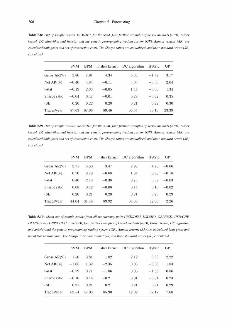
106 Chapter 5. Forecasting
Table 5.8: Out of sample results, DEM/JPY, for the SVM, four further examples of kernel methods (BPM, Fisher
kernel, DC algorithm and hybrid) and the genetic programming trading system (GP). Annual returns (AR) are
calculated both gross and net of transaction costs. The Sharpe ratios are annualized, and their standard errors (SE)
calculated.
SVM BPM Fisher kernel DC algorithm Hybrid GP
Gross AR(%) 3.80 7.91 4.34 6.33 −1.47 3.17
Net AR(%) −0.40 4.84 −0.11 3.03 −6.36 2.04
t-stat −0.19 2.33 −0.05 1.45 −3.06 1.34
Sharpe ratio −0.04 0.47 −0.01 0.29 −0.62 0.35
(SE) 0.20 0.22 0.20 0.21 0.22 0.30
Trades/year 87.63 67.96 89.46 66.54 99.13 23.39
Table 5.9: Out of sample results, GBP/CHF, for the SVM, four further examples of kernel methods (BPM, Fisher
kernel, DC algorithm and hybrid) and the genetic programming trading system (GP). Annual returns (AR) are
calculated both gross and net of transaction costs. The Sharpe ratios are annualized, and their standard errors (SE)
calculated.
SVM BPM Fisher kernel DC algorithm Hybrid GP
Gross AR(%) 2.71 5.50 3.47 2.95 4.75 −0.06
Net AR(%) 0.70 3.79 −0.68 1.34 0.93 −0.18
t-stat 0.40 2.13 −0.38 0.75 0.52 −0.03
Sharpe ratio 0.08 0.42 −0.08 0.14 0.10 −0.02
(SE) 0.20 0.21 0.20 0.21 0.20 0.29
Trades/year 44.04 31.46 89.92 38.33 82.00 2.26
Table 5.10: Mean out of sample results from all six currency pairs (USD/DEM, USD/JPY, GBP/USD, USD/CHF,
DEM/JPY and GBP/CHF) for the SVM, four further examples of kernel methods (BPM, Fisher kernel, DC algorithm
and hybrid) and the genetic programming trading system (GP). Annual returns (AR) are calculated both gross and
net of transaction costs. The Sharpe ratios are annualized, and their standard errors (SE) calculated.
SVM BPM Fisher kernel DC algorithm Hybrid GP
Gross AR(%) 1.50 3.81 1.82 2.12 0.83 2.22
Net AR(%) −1.65 1.32 −2.35 0.03 −3.38 1.83
t-stat −0.79 0.71 −1.06 0.03 −1.56 0.86
Sharpe ratio −0.16 0.14 −0.21 0.01 −0.31 0.23
(SE) 0.21 0.21 0.21 0.21 0.21 0.29
Trades/year 62.54 47.03 85.90 42.02 87.17 7.68

5.5. Testing 107
Conclusion
The mean gross returns from all six experiments were positive, with the BPM being significantly higher
than the others, and the hybrid algorithm the lowest. The mean net returns and Sharpe ratios were
significantly positive for the GP methodology and the BPM, but negative for the SVM, Fisher kernel
and the hybrid algorithm. The BPM and DC algorithm were improvements over the vanilla SVM in
terms of gross return, net return and Sharpe ratio, whilst the Fisher kernel was an improvement over the
vanilla SVM in terms of gross returns. Overall, BPM had the highest gross return, but GP had the highest
net return and Sharpe ratio. One likely reason for the superior performance of the genetic programming
methodology is that it was better suited to optimally restricting the number of trades per year. The hybrid
algorithm and the Fisher kernel generated the most trades per year, whilst GP generated the fewest trades.
However, the performance of the genetic programming trading system described in Neely et al. (1997)
was one of the worst reported in Neely et al. (2009). The following three methods performed best.
Sweeney (1986) used filter rules, as described in Fama and Blume (1966). Taylor (1994) considered
ARIMA(1,0,2) trading rules, prespecifying the ARIMA order and choosing the parameters and the size
of a ‘band of inactivity’ to maximize in-sample profitability. Dueker and Neely (2007) used a Markov-
switching model on deviations from uncovered interest parity, with time-varying mean, variance, and
kurtosis to develop trading rules; again, in-sample data was used to estimate model parameters and to
construct optimal ‘bands of inactivity’ that reduce trading frequency. The filter rules and ARIMA trading
systems are both linear in nature, whilst the Markov-switching model is non-linear but utilises higher
moments. It could be that applying kernel methods, a non-linear technique used with straightforward
average returns and interest rate differentials as inputs in this instance, led to overfitting the training set,
and that choice of the correct inputs, rather than the kernel, was crucial.
Recall that the no free lunch theorem for supervised learning (Section 2.5.1) informs us that, where
d = training set, m = number of elements in training set, f = ‘target’ input-output relationships, h =
hypothesis (the algorithm’s guess for f made in response to d) and c = off-training-set ‘loss’ associated
with f and h (‘generalization error’ or ‘test set error’), if you make no assumptions about the target
functions, or if you have a uniform prior, then P (c|d) is independent of one’s learning algorithm. Vapnik
(1999) appears to ‘prove’ that given a large training set and a small VC dimension, one can generalize
well. The VC dimension is a property of the learning algorithm, so no assumptions are being made about
the target functions. So, has Vapnik found a free lunch? VC theory tells us that the training set error, s,
converges to c. If ε is an arbitrary real number, the VC framework actually concerns
P (|c− s| > ε|f,m).
VC theory does not concern
P (c|s,m,VC dimension).
So there is no free lunch for Vapnik, and no guarantee that SVMs (or any kernel methods) generalize
well. We noted at the start of the chapter that the kernel defines a similarity measure between two data
points and thus allows one to incorporate prior knowledge of the problem domain. The problem with

108 Chapter 5. Forecasting
financial markets, as we have seen, is that we have very little useful domain knowledge.
I would expect the returns generated by all of the models to diminish with time, especially as they
are published, and would not be confident that significant profits could be made in today’s market.
5.6 Conclusion and Summary
The chapter began with an experiment involving forecasting DJIA daily returns. It continued with expla-
nations of kernel methods and support vector machines. The importance of preprocessing one’s data was
discussed and the methods used, namely normalization and avoiding multicollinearity, were highlighted.
The methodology regarding model selection and feature selection was described and the software in-
troduced. Many trading systems were built, which traded large cap US stocks intra-day, FTSE 100
constituents daily, US stocks weekly, FTSE 100 constituents monthly, US stocks daily with fundamental
inputs, commodities daily and FX daily, although to save space, only the experiments on the final data
set are reported. The applications of the Fisher kernel, the DC algorithm and Bayes point machine to
financial time series are all new. Most novel of all was the use of the DC algorithm to learn the parame-
ters of the hidden Markov model in the Fisher kernel. Table 5.11 gives a summary of the goals achieved
Table 5.11: Summary of results on forecasting
Beat standard SVM? Yes
Beat state of the art? No
in the forecasting chapter of this thesis. More precise conclusions are elusive, because a slight change
to the data set or the inputs can produce quite different results. Although I believe that machine learn-
ing in general, and learning the kernel in particular, have a lot to offer financial time series prediction,
financial data is a poor test bed for comparing machine learning algorithms due to its vanishingly small
signal-to-noise ratio.

109
Chapter 6
Assessment
This chapter undertakes a critical assessment of the work by restating the hypothesis (Sec-
tion 6.1), demonstrating the precision (Section 6.2) and thoroughness (Section 6.3) of the
work on the characterization, modelling and forecasting of financial time series, restating
the contributions (Section 6.4) and providing a comparison with the work of others that is
most similar to my own (Section 6.5). The chapter ends with a conclusion and summary
(Section 6.6).
6.1 Hypothesis
Recently, a great deal of machine learning has been applied to the area of bioinformatics, and the area
appears to drive the research within kernel methods. Meanwhile, the application of machine learning to
the financial domain is of a much lower quality (pp. 49–52). There is ample scope for the application of
novel kernel methods to financial markets. It was hypothesized that the state of the art in financial time
series analysis could be improved upon by applying machine learning. Although, in the case of the work
on forecasting (Chapter 5) the aims were graduated thus: 1) to improve standard algorithms, and 2) to
beat the ‘state of the art’.
I utilized the time series trichotomy given in Gershenfeld and Weigend (1994) and applied it to
financial time series to structure the core of the thesis thus: characterization (Chapter 3), modelling
(Chapter 4) and forecasting (Chapter 5).
characterization Characterization attempts with little or no a priori knowledge to determine fundamen-
tal properties, such as the stationarity of a system or the amount of randomness.
modelling The goal of modelling is to find a description that accurately captures features of the long-
term behaviour of the system.
forecasting The aim of forecasting (also called predicting) is to accurately predict the short-term evolu-
tion of the system.

110 Chapter 6. Assessment
The major time series references were given in Section 2.3.2 (p. 30) and a glossary is provided in Ap-
pendix C (p. 141–142).
The thesis research question is: ‘Can one improve upon the state of the art in financial time series
analysis through the application of machine learning?’
6.2 Precision
One should expect a peculiar (non-linear) publication bias in the areas covered in this thesis: the efficient
market hypothesis, technical analysis and trading systems. In general, and in common with all other ar-
eas of research, positive results are more likely to be published, which in the case of trading systems,
technical analysis and behavioural finance, means evidence against the EMH. However, those with a
vested interest in supporting the existing paradigm (the EMH) and those with results that are so good
that they would rather keep them to themselves are less likely to publish results that highlight market
inefficiencies. Furthermore, as academics seek to make a novel contribution there will likely be a bias
towards publications showing novel algorithms outperforming established algorithms. For an interest-
ing and short paper on publication bias/positive outcome bias/the ‘file-drawer problem’, see Rosenthal
(1979). Ioannidis (2005) claims that most published research findings are false. Assuming that his paper
is itself correct, problems with experimental and statistical methods mean that there is less than a 50 per
cent chance that the results of any randomly chosen scientific paper are true. The reasons for this include
small sample sizes, poor study design, researcher bias and selective reporting. Although I strive to avoid
such biases, I cannot guarantee that I am totally immune.
Characterization
For the characterization of financial markets as much data as possible was used. The DJIA was chosen as
it is the best-known and second-oldest US stock index, the data set used spans over 83 years. Experiments
were conducted on daily, weekly, monthly and annual log returns, de-trended when necessary.
Modelling
The artificial stock market modelled in Chapter 4 replicated mean returns, the standard deviation of
returns, the absolute returns correlation and the squared returns correlation of a real stock market. How-
ever, the artificial stock market failed to accurately replicate the skewness, kurtosis and autocorrelation
of returns.
Forecasting
My foray into using kernel methods for forecasting foreign exchange rates produced mixed results. The
best of my models improved upon a standard support vector machine, but failed to match the genetic
programming methodology of Neely et al. (1997) published in Neely et al. (2009). More generally, it

6.3. Thoroughness 111
became apparent that attempting to predict individual financial time series is quite possibly a fruitless
exercise (especially at intermediate time horizons). One should always accept the only free lunch in
finance—diversification1—and trade a portfolio of assets, possibly using cointegration. It was after my
own prediction that FX markets are the least efficient (explained in Section 6.3 (p. 114)) that James
(2006) came to the same conclusion and claimed that only around 10 per cent of the market (the active
currency managers) are truly concerned with real returns.
I presented all of the results from my final experiments, and did not cherry-pick either favourable
results or data sets that show my algorithms in a favourable light.
6.3 Thoroughness
Characterization
For the characterization of financial markets four experiments—a test for autocorrelation, two runs tests
and a test for long memory—were conducted across four time intervals (daily, weekly, monthly and
annual), plus newsletters were analysed.
Modelling
The artificial stock market was built from the bottom up, at first utilizing evolutionary psychology, work
so detached from computer science that it was published separately (Sewell, 2011a).
Forecasting
The techniques employed, the simple trading algorithm used on the DJIA and the more complex kernel
methods, could be applied to any financial or commodity instruments. Of course, one can never guaran-
tee that a system will generate certain returns above the risk-free rate. If one could, given capital, leverage
and enough time, one would eventually own the entire world. One can never be sure that one’s trading
system will perform successfully in the future at all. The nature of the markets could change overnight.
One cannot predict events such as the ‘September 11 attacks’ in 2001. However, the assumption behind
technical analysis (presumably due to aspects of behavioural finance) is that the markets react after the
event in a predictable way. If the model fails on the test set, then one must conclude that either the time
series is unpredictable or the preprocessing and/or prediction methodology were not suited to the task.
What follows are some questions and answers that should be of interest to a market practitioner. The
website Quantpedia2 analyses trading strategies documented in the academic literature, and should also
be of interest.
1Modern portfolio theory (MPT) dictates that the only free lunch in finance is diversification.2http://quantpedia.com/

112 Chapter 6. Assessment
Is it worth trying to predict financial markets?
If a market is weak-form efficient, then technical analysis will fail. If a market is semi-strong-form
efficient, then both technical analysis and fundamental analysis will fail. For a discussion of efficient
markets, see Section 2.1 (pp. 27–29). Just under half of the papers reviewed in my review of the efficient
market hypothesis (Sewell, 2011e) support market efficiency, whilst around 30 per cent of the relevant
articles reviewed in my review of fund performance (Sewell, 2011d) supported market efficiency. After
a century of analysis, there is no clear consensus, and I reject notions that the EMH is clearly true, or that
the EMH is clearly false and work with the assumption that market efficiency is relative, not absolute.
Recall that a market is said to be efficient with respect to an information set if the price ‘fully reflects’
that information set (Fama, 1970). On the one hand, the definitional ‘fully’ is an exacting requirement,
suggesting that no real market could ever be efficient, implying that the EMH is almost certainly false.
On the other hand, economics is a social science, and a hypothesis that is asymptotically true puts the
EMH in contention for one of the strongest hypotheses in the whole of the social sciences. Strictly
speaking the EMH is false, but in spirit is profoundly true. Besides, science concerns seeking the best
hypothesis, and until a flawed hypothesis is replaced by a better hypothesis, criticism is of limited value.
Due to imperfect arbitrage opportunities and correlated irrational behaviour, I take the view that it is
worth trying to predict financial markets due to the potential for high rewards and the enhanced mate-
value it provides men (Moxon, 2008; Sewell, 2008b), but recognise that the task is extremely difficult
and that the majority of people fail.
What skills are required?
The task of predicting markets should be approached with scientific and statistical rigour. In addition to
robust scientific methods, successful system building requires both creativeness (one wishes to identify
a signal which others have yet to find) and honesty (avoid data snooping). It is also crucial to attempt to
suppress one’s innate overconfidence and optimism.
What is one trying to do?
The no free lunch theorem for supervised machine learning (see p. 47) proves that, under some fairly
general conditions, all algorithms are equivalent, on average. In other words, the success of an algorithm
says as much about the data as about the algorithm. What’s more, the data of interest here—financial
time series—is extremely noisy. The best one can hope for is an algorithm that generalizes well on the
data sets of interest. This is achieved by creating an algorithm that successfully exploits one’s intuitive
implicit prior knowledge concerning P(target) so that it implicitly assumes a P(hypothesis | training set)
which is aligned with P(target | training set), where ‘hypothesis’ is one’s guess for the ‘target’ input-
output relationships. In short, one must use their prior knowledge to determine the machine learning
bias. SVMs in general assume smoothness priors. Here, domain knowledge has been used to facilitate
shrewd subset selection, feature selection and the preprocessing of the data.

6.3. Thoroughness 113
What assumptions are being made?
With financial time series, there is little domain knowledge (although, thanks to my review of the litera-
ture on the characteristics of financial markets (Sewell, 2011b), this thesis uses as much as possible), so
one must make do with fairly minimal assumptions. Induction relies upon ‘The principle of uniformity
of nature’, which Hume (1748) summed up with the phrase ‘For all inferences from experience suppose,
as their foundation, that the future will resemble the past, and that similar powers will be conjoined with
similar sensible qualities.’ The author of this thesis—like all technical analysts—makes the assumption
that the future signal will be like the past. It is also assumed that the universe is smoother than ran-
dom. When it comes to feature selection, ‘Tobler’s first law of geography’ is employed (see Section 5.3
(p. 87)).
Which algorithm should one use?
A trading system must identify the relationship between the mean of a dependent variable (log returns)
and one or more ‘independent’ variables (technical (and sometimes fundamental) inputs), i.e. perform
(possibly non-linear) regression. One may also use classification, and classify the market into ‘up’ or
‘down’ movements, as in this thesis. Certainly, this thesis recommends using a data-driven approach
by employing machine learning. Using both theory and domain knowledge, one must, a priori, select a
prediction technique. Neftci (1991) showed that technical analysis relies on non-linearities being present.
There is ample empirical evidence that a non-linear process contributes to the dynamics of market returns
(Hsieh, 1989; Scheinkman and LeBaron, 1989; Brock et al., 1991). In their review paper, Park and Irwin
(2004) found that, on average, non-linear methods outperformed genetic programming in all three types
of market considered: stock markets, futures markets and currency markets. How does a support vector
machine compare with its close rival, an artificial neural network (ANN)? Firstly, it should be made
clear that SVMs contain a large class of neural networks and radial basis function (RBF) networks as
special cases. The development of ANNs followed a heuristic path, with applications and extensive
experimentation preceding theory. In contrast, the development of SVMs involved sound theory first,
then implementation and experiments. A significant advantage of SVMs is that whilst ANNs can suffer
from multiple local minima, the solution to an SVM is global and unique. Two more advantages of SVMs
are that they have a simple geometric interpretation and give a sparse solution. Also, unlike ANNs, the
computational complexity of SVMs does not depend on the dimensionality of the input space. ANNs
use empirical risk minimization, whilst SVMs use structural risk minimization. The reason that SVMs
often outperform ANNs in practice is that they deal with the biggest problem with ANNs, SVMs are less
prone to overfitting. In addition to the theoretical reasons for preferring support vector machines over
neural networks, there are empirical reasons. Of the 36 articles in the literature review on pp. 49–52
that compare SVMs with ANNs when applied to financial or commodity markets, SVMs outperformed
ANNs in 28 cases, ANNs outperformed SVMs in 4 cases, and there was no significance difference in
4 cases. In light of these findings, this author settled for support vector machines as the prediction tool
of choice. SVMs are related to smoothness priors, so satisfy that assumption. On a separate note, the

114 Chapter 6. Assessment
nature of trading dictates that the most profitable algorithm may well be one that identifies a trend.
Which markets should one predict?
For reasons of market efficiency, a priori, one would assume that there is no privileged market. As
explained in Table 2.1 (p. 31), due to risk aversion, investors require a small positive expected return
in risky markets. In long-only markets—like a stock market—this implies a positive upward drift. In
symmetric markets which traders are as likely to be long as they are short, like futures and foreign
exchange markets, the implication is that one would expect the price to be predictable to some degree.
Furthermore, government intervention in foreign exchange markets may provide a positive sum game
for other participants in the short-term (Neely, 1998; LeBaron, 1999; Neely and Weller, 2001). So,
for theoretical reasons, one may expect that foreign exchange markets should be the most predictable,
futures markets intermediate and stock markets the least predictable. The empirical evidence found in
Park and Irwin (2004) and James (2006) confirms this theory. However, a buy-and-hold strategy in the
stock market should make money because stock markets are a positive sum game, whilst the same cannot
be said for futures or FX markets. Costs in futures and FX markets are tiny; FX is the lowest with $1m of
notional costing $3 to trade, whilst futures costs are considerably less than one tick. Costs are dominated
by the spread.
At what time frame should one predict?
Again, for reasons of market efficiency, a priori, one would assume that there is no privileged time
frame. The world’s most successful hedge funds trade at both ultra-high frequencies (Renaissance Tech-
nologies) and over the very long-term (Warren Buffett). The former employ technical analysis, and this
is consistent with the literature that finds evidence of dependence at the tick level, but not at longer time
horizons (p. 32–34). Buffett employs fundamental analysis, but my analysis of the dependence of annual
returns in Chapter 3 implies that technical analysis should work over the long-term too. Like business
in general, finding a niche is ideal. If one has the luck and skill of Warren Buffett, one should trade
long-term using fundamental analysis; if one is of a quantitative bent and able to invest heavily in IT,
one should trade short-term using technical analysis.
Conrad and Kaul (1998) implemented and analysed a wide spectrum of trading strategies during
the 1926–1989 period, and during subperiods within, using the entire sample of available NYSE/AMEX
securities. They found that a momentum strategy is usually profitable at the medium (3- to 12-month)
horizon, while a contrarian strategy nets statistically significant profits at long horizons, but only during
the 1926–1947 subperiod. This implies that markets exhibited both persistence and antipersistence, at
different time periods, providing an explanation for the success of trading systems in the past, and hope
for the success of systems in the future.
I include transaction costs as an integral part of the methodology, and changes in costs will effect
the frequency with which the systems optimally trade.

6.3. Thoroughness 115
Strategies
The strategies employed here fall under active investment management and are most likely to be em-
ployed by a hedge fund (described on p. 118) or the proprietary trading desk of an investment bank. The
financial industry use the term statistical arbitrage (also known as stat arb) to describe the computer-
generated ‘black box’ strategies used here. Any misgivings about such systems have more to do with the
illusion of control (Langer, 1975; Langer and Roth, 1975) (the tendency for people to overestimate their
ability to influence or control events) than any rational fear. A long/short strategy involves the combined
purchase and sale of two securities. A market neutral strategy is a long/short strategy that aims at bal-
ancing long and short positions to ensure a zero or negligible market exposure and consequently returns
that are independent of market movements. Market neutral strategies are pure alpha strategies. Note that
market neutral means beta neutral, not dollar neutral. An example of an equity market neutral strategy
is pairs trading, the combination of long and short positions that trade in the same market, are from the
same industry and from the same economic sector. Such strategies often rely on some form of mean re-
version. Mean reversion only requires one thing: that the mean exists. For example, the spread between
two stock prices may be stationary. Figure 6.1 shows the net market exposure of various strategies.
Figure 6.1: Net market exposure for various strategies in equities (Ineichen, 2002)
Finally, my review of the literature on fund performance (Sewell, 2011d) concluded that stock
picking is a worthwhile activity, whilst market timing is not; broadly speaking, this favours fundamental
analysis over technical analysis.

116 Chapter 6. Assessment
Marketing
Beating the benchmark is only half the game in the real world: the other half is marketing. There is
no point in having a great strategy if one is unable to raise enough funds to implement it profitably.
It is worth noting that the marriage of strategies and marketing has generated some terminology and
methodology which deserves closer examination. Firstly, the expression statistical arbitrage conjures
up images of robustness (from ‘statistics’) and risk free (from ‘arbitrage’), whilst the reality is that sta-
tistical arbitrage is simply gambling in the markets. Although there is an investor–speculator continuum
with someone who holds cash and is long the entire market being the only pure investor, and at least
stat arb is gambling with a positive edge. A strategy may be market neutral, and marketed as such so
that the potential investor can then invest a portion of their wealth accordingly; whilst the constraints
(and resultant transaction costs) would likely compromise expected returns to a greater extent than a less
restrictive strategy. The Sharpe ratio is a popular but flawed performance metric which is open to ma-
nipulation (see p. 77). Drawdowns are another favourite method of evaluating performance (no one likes
losing money), but the metric relies upon two assumptions (both of which must be satisfied for the use
of drawdowns to make sense). Firstly, drawdowns must describe the risk-preferences of the investor and
secondly the returns from the trading system must not be independent (if the returns are independent, the
shape of the curve is irrelevant). In practice, the second assumption implies that the magnitude of the
signal in the market displays persistence, plus the trading system’s predictions are not conditioned on
the magnitude of said signal. Using maximum drawdown does make sense, however, when maximum
drawdown is calculated repeatedly for a bootstrapped sample. The busy manager’s favourite is the equity
curve, the idea being that he has neither the time nor the ability to examine the strategy (and everyone
likes a picture); again, it only makes sense under assumptions very similar to those under which the use
of drawdowns makes sense. Stop-losses may appear to mirror investors’ risk preferences, but in practice
are often an example of pandering to marketing. The use of stop losses only enhances returns under the
assumption of persistence in the market. An assumption that is wrong as often as it is right (Conrad and
Kaul (1998) show that this is the case, albeit over long time intervals). All of the above practices neces-
sarily decrease expected returns, but may be consistent with investors’ risk preferences. Also amusing is
the story-telling that takes place, allegedly, to explain why a trading system stops working. The assump-
tion here is that the system worked in the first place, when in reality they may have simply been lucky,
and their luck ran out. I am myself guilty of some of the points I’ve outlined. I take the view that any
financial time series is close to a martingale, and any trading algorithm must be explained in terms of
how the market deviates from a martingale. Of course, this process may take place implicitly.
6.4 Contributions
The contributions made are listed below.
Experiment 1: Characterization
• I reconciled the apparent efficiency of markets according to linear statistical tests (e.g. auto-

6.4. Contributions 117
correlation) with the potential for non-linear forecasting methods to generate above-average
risk-adjusted returns and identified the nature of inefficiencies (Chapter 3). An analysis of
DJIA and foreign exchange log returns using the runs test, that detects linear and non-linear
relationships, identified several previously undocumented anomalies: daily DJIA, USD/-
DEM, USD/JPY, GBP/USD, USD/CHF and GBP/CHF returns each exhibit a surprisingly
high number of sequences of decreasing returns.
• I wrote software for performing the runs test in Visual Basic for Excel (Section 3.3). I also
wrote software for testing for long-memory, rescaled range analysis, in C++ and Visual Basic
for Excel (Section 3.4). Neither algorithm was previously available for free as downloadable
software including source code. The runs test source code is given in Appendix D and the
rescaled range analysis source code is given in Appendix G.
Experiment 2: Modelling
• A novel investment performance measurement metric, cumulative prospect theory certainty
equivalent (CPTCE), was developed from Tversky and Kahneman’s cumulative prospect
theory. The statistic models investors’ empirically-observed risk preferences (people care
about losses and gains rather than absolute wealth, evaluate probabilities incorrectly, are loss
averse, risk averse for gains, risk seeking for losses and have non-linear preferences), whilst
no other performance metric does this effectively. The financial industry have taken interest,
with offers to commercialize the product. See Section 4.2.
• The evolved heuristics and biases exhibited by fundamental analysts and technical analysts,
inducing underreaction and overreaction, were used to build an agent-based artificial stock
market. The resultant time series replicates mean returns, the standard deviation of returns,
the absolute returns correlation and the squared returns correlation of a real stock market,
and provides a novel insight into the effect of the proportion of technical analysts relative to
fundamental analysts. See Section 4.1.
Experiment 3: Forecasting
• Two Windows implementations of SVMs with semi-automated parameter selection were
built. SVMdark is based on SVMlight and written in C for Win32, whilst winSVM is based
on mySVM and written in C++ for Win32. For some time the programs were the only Win-
dows applications dedicated to support vector machines, they were frequently downloaded
and have been used by the financial industry. The source code is also freely available to
download. See p. 87.
• A (generative) hidden Markov model was trained on market data to derive a Fisher kernel for
a (discriminative) support vector machine, the DC algorithm and a Bayes point machine are
also used to create kernels. Furthermore, the DC algorithm was used to learn the parameters
of the hidden Markov model in the Fisher kernel, which is a novel combination of algorithms.

118 Chapter 6. Assessment
All four algorithms performed better than the vanilla SVM in terms of gross returns, net
returns and Sharpe ratio. See Chapter 5.
The reason that this area of research is profound is that machine learning can be viewed as an
attempt to automate ‘doing science’.
To whom is this thesis useful? Outside academia, the contributions are most likely to be of interest
to the alternative investment industry. A hedge fund is an ‘alternative investment’ fund that aims to
maximize absolute returns, charges high fees and pursues high risk investment strategies. In 1949 Alfred
Winslow Jones established the first hedge fund. His inspiration came from the research he was doing
for an article he was writing for Fortune about technical methods of market analysis (Jones, 1949). He
raised $100,000 (including $40,000 of his own capital) and started an equity fund. Jones’s innovation
was to merge two known speculative tools: short sales and leverage. Hedge funds remained relatively
obscure until the structure and success of Jones’s fund was covered by Carol Loomis in another article
in Fortune (Loomis, 1966). The accelerating growth of hedge funds between 1980 and the 2008 credit
crunch was phenomenal. Regardless of whether markets are (increasingly) efficient, the growth in hedge
funds indicated that the desire to invest in actively managed funds was growing, not diminishing. Today,
hedge fund strategies broadly fall within four areas: long/short, relative value/arbitrage, event-driven and
directional. I run a hedge fund portal dedicated to academic research.3 For more on hedge funds, see the
primer Lhabitant (2002) or the more comprehensive Lhabitant (2006).
6.5 Comparison with Similar Work of Others
I’ve given my contemporaries working in the same area as much help as possible, by making much of the
content of this thesis available online. Readers with access to a soft copy of this thesis should appreciate
the full hyperlinking, both internal cross referencing and externally linking most of the 450+ items in the
bibliography to articles on the Web.
Characterization
There is plenty of empirical work on the statistical nature of financial markets, but few good all-inclusive
review papers. Cont (2001) is probably the best review paper of stylized facts in financial markets in
general, whilst Guillaume et al. (1997) gives a review of the foreign exchange market.
Modelling
The best known models of financial time series are autoregressive conditional heteroskedasticity
(ARCH, Engle (1982)) and generalized autoregressive conditional heteroskedasticity (GARCH, Boller-
slev (1986)) processes. The work here does not attempt to compete with such models in terms of an
accurate statistical description of financial markets.
3http://www.edge-fund.com

6.5. Comparison with Similar Work of Others 119
Barberis et al. (1998), Daniel et al. (1998), Hong and Stein (1999), Veronesi (1999) and Lee and
Swaminathan (2000) all present very good models of markets which exhibit both underreaction and
overreaction (see p. 41 for details). Again, the relevant work here does not attempt to compete with these
models in terms of their explanation of market under- and overreaction.
Martinez-Jaramillo (2007) and Martinez-Jaramillo and Tsang (2009) developed an artificial finan-
cial market and modelled technical, fundamental and noise traders. They investigated the different condi-
tions under which the statistical properties of an artificial stock market resemble those of a real financial
market. Their approach replicated the stylized facts of a financial market far more accurately than my
own; this was possible by including and adjusting a much larger number of parameters. They also inves-
tigated the effects on the market when the agents learn, whilst in my model, by design, no learning takes
place. On average, their model without learning replicated the stylized facts most accurately, but not by
much (Martinez-Jaramillo (2007), Table 6.5).
Forecasting
Trading systems for equity and commodity markets which trade at various time scales have been built
using support vector machines with varying degrees of success, some of which are reported here. It is
hypothesized that using SVMs on financial time series is more effective than linear regression (due to
non-linearities in the market) and neural networks (due to overfitting). Due to the necessarily secretive
nature of the financial industry, little is known of the methodology in use by the most successful sys-
tematic traders. However, one is generally aware of their performance. Certainly, I do not pretend to
compete with the best in the world on that basis. For example, Renaissance Technologies’ (who also em-
ploy a scientific approach to trading) Medallion Fund has averaged approximately 35 per cent annualized
net returns since its 1988 inception (Zuckerman, 2013). The ultimate test: would I trade my systems?
Currently, no; but with access to more data, processing power, experience and time I reserve the right to
be optimistic about the future. As mentioned earlier, the no free lunch theorem for supervised machine
learning (p. 47) dictates that, under some fairly general conditions, all algorithms are equivalent, on av-
erage. Therefore the comparison of algorithms in a general setting is futile. The best one can hope for is
that their algorithms (implicitly) exploit prior knowledge in the form of a learning bias more effectively
than the competition.
The performance metric, cumulative prospect theory certainty equivalent (CPTCE), is new to the
domain of finance. As a descriptive measure of people’s attitude towards risk, it should be superior to
any other existing measure, even allowing for seemingly irrational behaviour such as simultaneously
purchasing insurance and lottery tickets. As a prescriptive description of how people should invest,
something like the trade-off between an optimal growth strategy and the security of holding cash advo-
cated by MacLean et al. (1992) or the iterated log function described in McDonnell (2008) would likely
be better.

120 Chapter 6. Assessment
Thesis
Taken as a whole, how does the thesis compare with similar work by others? The fast pace of computer
science makes anything other than recent comparisons unfair. I have compiled a list of publications that
in some ways may be considered to be similar to my own in Appendix L (p. 189–190).
Below, the approach of the discipline used here, machine learning, is contrasted with other ap-
proaches.
Commercial world According to Nassim Nicholas Taleb4, while Wall Street research departments may
be way ahead of academia in pure derivatives pricing (and other abstractions), they, surprisingly,
lag in the more relevant area of quantitative empiricism. Hedge funds are notoriously secretive, so
little is know of their strategies.
Engineering Engineers take a robust and pragmatic approach, but care is needed to avoid the over-
enthusiastic application of an engineer’s tools. For example, whilst the Kalman filter is frequently
applicable in the physical world, the assumptions on which it is built (linear and Gaussian) are not
relevant to financial time series. Having said that, one always has to make some assumptions.
Economics The Victorian historian Thomas Carlyle gave economics the nickname ‘dismal science’. In-
deed, the various schools of economic thought are ideologies, and all ideologies are false (Sewell,
2012d). In particular, economics is often criticised for being founded upon dubious assumptions
of rationality, unrealistic risk preferences and fanciful normally distributed returns (see, for exam-
ple, the capital asset pricing model (CAPM) (Treynor, 1962; Sharpe, 1964; Lintner, 1965; Mossin,
1966)). You may have heard the joke about the three hungry castaways on a deserted island who
are trying to open a can of food. The physicist proposes breaking it open with a sharp rock, the
chemist suggests heating the can until it bursts, and the economist says ‘Assume we have a can
opener. . . ’.
Econometricians seem obsessed with linear regression analysis. The optimal nature of least
squares linear regression is often justified by the Gauss-Markov theorem, which rests on the
assumption of linearity, which itself rests on little. This is an important point because outside
quantum mechanics, no model of a real system is truly linear (Meiss, 2003). Having said that,
a linear model may still be useful for modelling a non-linear process. For example, the simplest
non-trivial model obtainable from the Taylor expansion of any infinitely-differentiable function is
a linear model (the first-order expansion of the Taylor series).
Economics is unique among the human and social sciences in that it is egalitarian. It starts from
the premise that all races, social groups, societies and individuals are created equal, i.e. have equal
potential. Economists speak of ‘developing nations’ and ‘developed nations’, there is never any
question of whether or not the developing nations will one day be developed, it is taken that they
will catch up. The problem with the assumption of egalitarianism is that scientific psychology and
4http://www.fooledbyrandomness.com/books.htm

6.5. Comparison with Similar Work of Others 121
work on intelligence shows that it is profoundly wrong. See, for example, Herrnstein and Murray
(1994), Lynn and Vanhanen (2002), Lynn and Vanhanen (2006), Lynn (2008) and Lynn (2015).
Physics Physics is a natural science and a physical science, whilst financial markets concern human
aspects of the world and are therefore better described as a social science. When tackling finance,
physicists tend to either shoehorn a social science into their own paradigm (e.g. modelling the
market using spin glass theory (Bornholdt, 2001)) or at the very least make unintuitive assumptions
(such as treating the market as a minority game (Challet et al., 2000)). A profound, yet often
overlooked, difference is that in physics there are constants and absolute sizes, whilst in economics
and finance there are not. For an introduction to ‘econophysics’, see Mantegna and Stanley (2000).
As an aside, I often wonder if encouraging physicists (the brightest of us all (Motl, 2006)) into the
financial domain (which simply moves money around) is such a good idea, as they could be doing
something more productive with their skills.
Statistics The statistical community generally assume that the data are generated by a given stochastic
data model (Breiman, 2001). This is not appropriate for, in particular, short term financial fore-
casting because the data is produced by a complex and largely unknown process, and our goal
is prediction, not interpretability. Furthermore, we are not so much concerned with validating a
model as formulating the process of generalization by searching for the best model (Witten et al.,
2011, pp. 28–29).
Machine learning The task of forecasting financial markets is one of predicting a time series generated
from a social science, which in practice may be considered as purely an exercise in information
processing. This was achieved by making minimal assumptions and using a data-driven, model-
free, flexible and nonparametric approach. In other words, I used machine learning, in the guise of
supervised learning, which encompasses both theoretical soundness and experimental effective-
ness. Multiagent systems were the most natural way of modelling a market with many agents.
Being a relatively fast changing discipline, computer science can be rushed, which naturally com-
promises quality. Also, computer scientists are far too overconfident and optimistic, seemingly
unaware just how efficient markets are. My other main criticism is that a lot of the machine learn-
ing community tend to champion their favourite technique, which in practice results in a solution
looking for a problem. There is also the temptation for researchers in academia to treat machine
learning as an exercise in searching for data sets that show their novel algorithm in a favourable
light (in practice, the no free lunch theorem for supervised learning (see p. 47) makes this in-
evitable). Also, often simple solutions (such as linear regression) are overlooked. Other criticisms
include the irrelevance of fuzzy logic (see Lindley (1987)) and the intellectual dishonesty of the
evolutionary and supervised learning communities. The former often (implicitly) deny the no free
lunch theorems, whilst the latter regularly fail to declare what events their probabilities are con-
ditioned on (e.g. Vapnik (1982), Vapnik (1998) and Vapnik (1999) are guilty of this sin). Despite
these grievances, on balance, I recommend the machine learning paradigm above all others, but

122 Chapter 6. Assessment
use with care and common sense. Although due to the low signal-to-noise ratio of financial mar-
kets it is possible that they are not a great test bed for new algorithms. That is, computer science
has a lot to offer finance, but the converse is not true.
To conclude:
• Machine learning offers a flexible approach to financial time series analysis.
• The scope of the thesis is unusual.
• The thesis makes inter-disciplinary contributions.
6.6 Conclusion and Summary
The work undertaken during the course of this thesis is important across various disciplines. The use
of the DC algorithm to learn the parameters of the HMM in the Fisher kernel is a novel algorithmic
contribution to computer science, whilst my support vector machine software for Windows has proved
popular and introduced SVMs to a wider audience. The investment performance measurement metric I
developed, CPTCE, is in use by, and is truly beneficial to, the financial industry. My genuinely novel
work on the evolutionary foundations of heuristics and biases (Sewell, 2011a) (not reported here) should
be of great interest to psychologists.
Should the thesis be judged from an engineering perspective, here lies a summary of the programs
written:
• Runs Test in Visual Basic for Excel
• Rescaled Range Analysis in C++ and Visual Basic for Excel
• Performance Measurement Calculator in PHP and Visual Basic for Excel
• Performance Metric Analysis in Visual Basic for Excel
• SVMdark in C for Win32
• winSVM in C++ for Win32
• Fisher Kernel in C++
• Monte Carlo Portfolio Optimization in Visual Basic for Excel
• Kelly Criterion in PHP and Visual Basic for Excel
• Order Book Reconstruction in C#

123
Chapter 7
Conclusion and Future Work
The final chapter starts with a conclusion that includes a summary of the thesis and the
contributions made, and finishes with ideas for extending the current work and several sug-
gestions for further work.
7.1 Conclusion
The central argument of the thesis is that one can improve upon the state of the art in financial time series
analysis through the application of machine learning. The results of the work on the characterization,
modelling and forecasting of financial time series each lend support to the central thesis. The research
question is answered in the affirmative. The following section concludes by summarizing the thesis and
highlighting the contributions made.
Summary
This thesis set out to do three things. It attempted to (1) characterize, (2) model and (3) forecast financial
time series using the best methods available to a computer scientist, in the hope that it is possible to
improve upon existing methodologies. Along the way, various contributions to both computer science
and other disciplines have been made.
Chapter 1: Introduction
This was a short chapter that ‘set the scene’. First, the research was motivated. Next, the research objec-
tives were given, and the research question stated, can one improve upon the state of the art in financial
time series analysis through the application of machine learning? ‘Financial time series analysis’ was
split into three areas: characterization (Chapter 3), modelling (Chapter 4) and forecasting (Chapter 5).
The research methodology was then provided for the three core chapters. Then the contributions to
science were given. Lastly, a chapter-by-chapter annotated guide to the thesis is provided.

124 Chapter 7. Conclusion and Future Work
Chapter 2: Background
The second chapter in the thesis details the work of others: it’s a survey and critical assessment of previ-
ous related work and its relation to the research in this thesis. The literature on the efficient market hy-
pothesis is reviewed quite thoroughly. For the research on characterization, following a note on markets,
the following areas are reviewed: time series, stochastic processes in financial markets, stylized facts,
dependence and long memory in market returns and investment newsletters. The blind alleys that we’ve
been led down (stable distributions, long memory in returns and chaos theory) were also highlighted,
and used as evidence for the importance of a data-driven approach. For the research on modelling, the
relevant literature on behavioural finance, technical analysis, multiagent systems, prospect theory and
investment performance measurement is reviewed. For the chapter on forecasting, the literature on the
no free lunch theorem for supervised machine learning, data snooping, kernel methods, SVMs vs ANNs
applied to the prediction of financial or commodity markets, and genetic programming is reviewed.
Chapter 3: Characterization
The chapter started with a description of the data used: the DJIA, six currency pairs and data from an
analysis of investment newsletters. Four analyses were conducted on stock market returns, and one on
investment newsletters. A test of autocorrelation plus two versions of the runs test showed that daily
DJIA, USD/DEM, USD/JPY, GBP/USD, USD/CHF and GBP/CHF returns each exhibit a surprisingly
high number of sequences of decreasing returns. Whilst an implementation of Hurst’s rescaled range
(R/S) analysis found little evidence of long memory in DJIA returns. Finally, an analysis of investment
letters was undertaken, and it was found that technical analysis performed poorly, evidencing weak-form
market efficiency, whilst fundamental analysis gave mixed results.
Chapter 4: Modelling
Two experiments are conducted, both utilize behavioural finance. In the first experiment, the evolved
heuristics and biases exhibited by fundamental analysts and technical analysts, inducing underreaction
and overreaction, are used to build an agent-based artificial stock market. Results showed that whether
a fundamental analyst, or a technical analyst, it pays to be in a majority. The artificial stock market
replicated mean returns, the standard deviation of returns, the absolute returns correlation and the squared
returns correlation of a real stock market, but failed to accurately replicate the skewness, kurtosis and
autocorrelation of returns. In a second experiment, risk preferences were modelled. A novel performance
metric, cumulative prospect theory certainty equivalent (CPTCE), was described and developed from
prospect theory.
Chapter 5: Forecasting
First, domain knowledge gained via the runs test was used to build a DJIA trading system. It could be
seen that, although the algorithm was created in sample, given its simplicity and the size of the data
set, significant overfitting of noise seems unlikely, so the equity curve is surprisingly impressive up until

7.1. Conclusion 125
2002, when the dynamics of the market must have changed. However, the algorithm clearly failed to
outperform the market in the out of sample period. Then kernel methods, support vector machines,
preprocessing, model selection, feature selection, SVM software and the Fisher kernel are introduced
and discussed. The Fisher kernel, the DC algorithm and the Bayes point machine were used to learn the
kernel on foreign exchange data. Most novel of all, the DC algorithm was used to learn the parameters of
the hidden Markov model in the Fisher kernel. The results were compared with both those of a standard
SVM and the published results from a genetic programming trading system. At best, they were superior
to the former, but not the latter. Two implementations of SVMs for Windows with semi-automated
parameter selection were built.
Chapter 6: Assessment
This chapter undertook a critical assessment of the work by restating the hypothesis, demonstrating
precision, thoroughness and contribution, and comparing the work with similar work by others. The
approach used in this thesis, machine learning, was contrasted with approaches taken by the commercial
world and the disciplines of engineering, economics, physics and statistics.
Chapter 7: Conclusion and Future Work
The current chapter concludes the thesis, and also addresses potential ideas for further work. Work which
is a direct extension to the work on characterization, modelling and forecasting financial time series is
considered. In addition, potential new avenues for the application of intelligent techniques are explored
which include algorithmic trading, cointegration, deep learning, ensemble learning, an equity trading
system, funds of funds, global macro strategies, market-making, merger arbitrage, money management,
option pricing, order book, particle filter and yield curve analysis.
The contributions made are listed below.
Experiment 1: Characterization
• I reconciled the apparent efficiency of markets according to linear statistical tests (e.g. auto-
correlation) with the potential for non-linear forecasting methods to generate above-average
risk-adjusted returns and identified the nature of inefficiencies in the DJIA (Chapter 3). An
analysis of DJIA and foreign exchange log returns using the runs test, that detects linear
and non-linear relationships, identified several previously undocumented anomalies. Daily
DJIA, USD/DEM, USD/JPY, GBP/USD, USD/CHF and GBP/CHF returns each exhibit a
surprisingly high number of sequences of decreasing returns.
• I wrote software for performing the runs test in Visual Basic for Excel (Section 3.3). I also
wrote software for testing for long-memory, rescaled range analysis, in C++ and Visual Basic
for Excel (Section 3.4). Neither algorithm was previously available for free as downloadable
software including source code. The runs test source code is given in Appendix D and the
rescaled range analysis source code is given in Appendix G.

126 Chapter 7. Conclusion and Future Work
Experiment 2: Modelling
• A novel investment performance measurement metric, cumulative prospect theory certainty
equivalent (CPTCE), was developed from Tversky and Kahneman’s cumulative prospect
theory. The statistic models investors’ empirically-observed risk preferences (people care
about losses and gains rather than absolute wealth, evaluate probabilities incorrectly, are loss
averse, risk averse for gains, risk seeking for losses and have non-linear preferences), whilst
no other performance metric does this effectively. The financial industry have taken interest,
with offers to commercialize the product. See Section 4.2.
• The evolved heuristics and biases exhibited by fundamental analysts and technical analysts,
inducing underreaction and overreaction, were used to build an agent-based artificial stock
market. The resultant time series replicates mean returns, the standard deviation of returns,
the absolute returns correlation and the squared returns correlation of a real stock market,
and provides a novel insight into the effect of the proportion of technical analysts relative to
fundamental analysts. See Section 4.1.
Experiment 3: Forecasting
• Two Windows implementations of SVMs with semi-automated parameter selection were
built. SVMdark is based on SVMlight and written in C for Win32, whilst winSVM is based
on mySVM and written in C++ for Win32. For some time the programs were the only Win-
dows applications dedicated to support vector machines, they were frequently downloaded
and have been used by the financial industry. The source code is also freely available to
download. See p. 87.
• A (generative) hidden Markov model was trained on market data to derive a Fisher kernel for
a (discriminative) support vector machine, the DC algorithm and a Bayes point machine are
also used to create kernels. Furthermore, the DC algorithm was used to learn the parameters
of the hidden Markov model in the Fisher kernel, which is a novel combination of algorithms.
All four algorithms performed better than the vanilla SVM in terms of gross returns, net
returns and Sharpe ratio. See Chapter 5.
7.2 Further Work
In this chapter potential ideas for further work in this field are addressed. If the field of research were
entirely efficient, there wouldn’t be any point in expending time and effort in seeking novel research, as
if it was viable, someone else would have already done it. Fortunately, perfect efficiency is impossible
(Grossman and Stiglitz, 1980). However, it is true that if I had thought of anything worth doing in the
allotted time, I would have already done it. Thankfully, a PhD takes a finite amount of time,1 so there is
always room for further work.
1Ex post.

7.2. Further Work 127
Firstly, logical extensions to the work covered in this thesis on the characterization, modelling and
forecasting of financial markets are considered. Secondly, this chapter explores further potential applica-
tions, further removed from the current work, but still within areas that could benefit from the ‘computer
science in finance’ paradigm, again with, whenever possible, an emphasis on machine learning.
Characterization
Despite the seriousness of the implications for risk and the willingness of many physicists to tackle the
problem, the precise distribution and scaling properties of financial time series returns is still an open
question. Both the size of available data sets and computing power can only increase, so even in the
unlikely event that there is no improvement in current methods of analysis, one should always be in an
increasingly better position to accurately characterize financial time series.
Modelling
Although not reported here, I did some research on the evolutionary foundations of heuristics (Sewell,
2011a). The fields of evolutionary psychology and behavioural finance are both relatively young and
growing. The intersection of the two fields is certainly ripe for future research. More specifically, an
attempt could be made to represent all six general purpose heuristics identified by Gilovich and Griffin
(2002) (affect, availability, causality, fluency, similarity and surprise) by introducing more parameters to
the artificial stock market. Further, some of the six special purpose heuristics also identified (attribution
substitution, outrage, prototype, recognition, choosing by liking and choosing by default) could be intro-
duced. The recognition heuristic (Goldstein and Gigerenzer, 1999, 2002), in particular, appears to be the
most accepted. As and when psychologists identify more heuristics and biases, one will be increasingly
able to capture the irrationalities of human behaviour in the model. Model validation is currently un-
satisfactory (although this is a problem with agent-based modelling in general, as highlighted on p. 65),
which leaves an obvious area for future work.
Forecasting
All methods of investment analysis are limited by the amount of data available; but supervised learning
suffers the most, so as the quantity and quality of available data increases, and the faster computers get,
the more of an edge systematic trading should have.
When building the trading systems, not every facet of the extensive literature review of stylized
facts has been utilized. If (say) a January effect were to exist and gradually become known, the only
way to profit from it would be to trade on the effect before fellow investors. As all investors strive to get
in before the crowd, the January effect would then become a December effect (there is indeed evidence
of a December effect (Chen and Singal, 2003)). Such a moving signal would require a more dynamic
approach to algorithm development.
Investors may wish to utilize the models as part of a larger portfolio. For this reason, a shrewd

128 Chapter 7. Conclusion and Future Work
investor would wish to know the distribution of returns of a trading system, or at least what strategy the
system employs. The distributions of returns could be analysed.
Volatility is non-stationary both in the short-term and the long-term. But what about the market
signal? Is volatility a proxy for noise? This is of interest because in support vector regression the
insensitivity parameter, ε, should vary linearly with the noise (Smola et al., 1998).
Regarding the work which involves the Fisher kernel, a great deal more experimentation is required
to optimise the various parameters, such as string length, number of symbols and number of states. Also,
this author believes that the real value of the Fisher kernel lies with its application to high frequency
trading where the structure of the order book comes into play. Future work on the DC algorithm-Fisher
kernel hybrid could involve increasing the efficiency of the algorithm (in practice, it was rather slow).
Renaissance Technologies’ Medallion Fund has achieved average annual returns of about 35It is
clearly worth attempting to mimic the strategy employed by such a successful fund. Like this author,
they use quantitative trading models. They trade with such high-frequency that their Nova fund accounts
for over 10 per cent of all the trades occurring on NASDAQ some days. Depending on transaction costs,
ultra-high frequency trading utilizing the order book looks attractive. Hopefully, more of the methods
outlined in this thesis will be used in the real world with real money.
New Directions
Potential new avenues of research are outlined below.
Algorithmic Trading
Market impact is the effect that a market participant has when they buy or sell an asset, it is the extent
to which the buying or selling moves the price against the buyer or seller, i.e. upward when buying and
downward when selling. A block trade is the sale or purchase of a large quantity of securities, normally
in excess of 10,000 shares. Due to the adverse market impact of block trades, algorithmic trading
developed, the aim of which is to split up the order in an optimal manner. The most common benchmark
is VWAP (volume-weighted average price), which is the ratio of the value traded to total volume traded
over a particular time horizon (usually one day). Machine learning could potentially be used to improve
algorithmic trading, specifically to alleviate the problem of market impact when placing large orders.
For example, Orchel (2011) successfully used an SVM for regression for an order execution strategy
with the goal of achieving VWAP by predicting volume participation.
Cointegration
Cointegration (Engle and Granger, 1987) is an econometric technique for testing the relationship be-
tween non-stationary time series variables. If two or more series each have a unit root, that is I(1), but a
linear combination of them is stationary, I(0), then the series are said to be cointegrated. For example, a
stock market index and the price of its associated futures contract, whilst both following a random walk,
will be in a long-run equilibrium and deviations from this equilibrium will be stationary. Robert Engle

7.2. Further Work 129
and Clive Granger shared the 2003 Bank of Sweden Prize in Economic Sciences in Memory of Alfred
Nobel, the latter’s portion due to his contribution to the development of cointegration. Alexander (2001)
points out that if the allocations in a portfolio are designed so that the portfolio tracks an index, then the
portfolio should be cointegrated with the index. She proposes that in a long-only fund one should track
log(index) + α, whilst I would extend this and define α as α = constant × standard deviation of log
returns over the training period. Secondly, triangular cointegration is (as far as I am aware) a novel idea
which may be employed whenever there exists a linear relationship between a linear combination of two
cointegrated assets and a third asset. The benefits include reduced transaction costs when compared to
ordinary cointegration because only the third asset is traded.
Deep Learning
Deep learning is a relatively new branch of machine learning that employs multiple processing layers in
order to learn representations of data with multiple levels of abstraction. It does so by using the back-
propagation algorithm to indicate how a machine should change its internal parameters that are used
to compute the representation in each layer from the representation in the previous layer (LeCun et al.,
2015). It has been found that unsupervised pre-training helps guide the learning towards basins of at-
traction of minima that support better generalization from the training data set—the pre-training appears
to act as a form of regularization (Erhan et al., 2010). Such methods have dramatically improved the
state-of-the-art in speech recognition, computer vision, natural language processing, audio recognition
and bioinformatics, and it seems likely that they may be fruitfully applied to the financial domain.
Ensemble Learning
Now that the author has completed an extensive literature review on ensemble learning (Sewell, 2011c)
and also has the ability to build several varieties of trading system, it is tempting to attempt to combine
their predictions in an optimal way. Ensemble methods are worth investigating further as they won the
Netflix Competition, KDD Cup 2009 and some of the Kaggle competitions (Demir, 2016).
Equity Trading System
Going back to basics, a rule-based equity trading system could be employed (after all, the signal may
turn out to be simple). The main advantage is that it would avoid the ‘black box’ nature of the other
predictive systems in this thesis, and so would have greater explanatory power.
Potential inputs to an equity trading expert system:
• Previous day’s performance of the stock (French and Roll, 1986)
• Previous week’s performance of the stock (Campbell et al., 1996)
• Previous month’s performance of the stock (Jegadeesh, 1990)
• Previous 9-month performance of the stock relative to the market (Conrad and Kaul, 1998)

130 Chapter 7. Conclusion and Future Work
• Previous day’s performance of the stock index (Campbell et al., 1996)
• Previous week’s performance of the stock index (Campbell et al., 1996)
• Previous month’s performance of the stock index (Campbell et al., 1996)
• Volume (Llorente et al., 2002)
• Day of the month (Ariel, 1987) (depending on the market (Kunkel et al., 2003))
• Month of the year (Rozeff and Kinney, 1976)
• Does the day precede a holiday? (Ariel, 1990)
Funds of Funds
A fund of funds is an investment partnership that invests in a series of other funds, the object being
to diversify. Intelligent techniques could be employed to select funds and allocate capital according
to various performance metrics. I have written a Monte Carlo simulation for portfolio optimization2,
which calculates mean return, standard deviation, skewness, kurtosis, beta, Jensen’s alpha, Sharpe ratio,
Sortino ratio, Treynor’s measure, information ratio, Stutzer ratio, Omega, M2, T2, maximum drawdown,
Cornish-Fisher-VaR, Mean of all Values and Value at Risk.
Global Macro Strategies
Global macro is a directional hedge fund strategy that invests globally based upon macro economic or
‘top-down’ analysis. Typified by George Soros’s Quantum Fund they have long been among the most
successful and most visible category of hedge funds. The ultimate ego trip, the strategy seeks to profit
by making leveraged bets on anticipated price movements of global stock markets, interest rates, foreign
exchange rates and physical commodities. Such strategies are not normally associated with quantitative
techniques. It is this author’s belief that they should be.
Market-Making
A market-maker is an intermediary who creates a market for a financial obligation. In a given market,
he must quote two prices: the lower is the bid (the price at which he is willing to buy) and the higher
is the offer (or ask) (the price at which he is willing to sell). The difference between an offer price and
the bid price is known as the spread. A market-maker receives the full order flow, so is in a unique
position to profit from the stream of data received. An automated market-making algorithm could be
designed using machine learning; it would need to accommodate the following three objectives: attract
order flow, control inventories and avoid losses to informed traders (‘adverse selection’). Limit orders are
disproportionately more likely to come from informed traders (Harris and Hasbrouck, 1996; Kaniel and
Liu, 2006). Bluffers are profit-motivated traders who try to fool other traders into trading unwisely; to
2Available from http://www.portfoliooptimization.co.uk.

7.2. Further Work 131
avoid losing to bluffers, market-makers must adjust their prices so that buy and sell orders have equal (but
opposite) market impact per quantity traded. If most traders use market orders, spreads will be narrow; if
most traders use limit orders, spreads will be wide. A market-maker may discover the equilibrium spread
by adjusting his spread so that limit orders and market orders are equally likely. Spreads increase with
(1) the degree of information asymmetry among traders, (2) volatility, and (3) utilitarian trading interest
(a utilitarian trader trades because they expect to obtain some benefit from trading besides profits). For
more details on ultra high frequency trading, see Sewell and Yan (2008).
Merger Arbitrage
Traditionally, merger arbitrage, also called risk arbitrage, concerns estimating the probability of a deal
being approved and how long it will take for the deal to close. There are many factors to consider. For
example, a deal may be friendly or hostile, and an offer can consist of shares, cash or debt, or any combi-
nation of the three. Furthermore, it is widely recognised that mergers come in waves that tend to coincide
with bull markets and economic growth. For background reading, the primer on hedge funds, Lhabitant
(2002), includes a chapter on event-driven strategies, and the more comprehensive Lhabitant (2006) a
chapter on merger arbitrage. For books specifically on merger arbitrage, see Wyser-Pratte (2009) (orig-
inally published in 1982), Moore (1999) and (by far the best) Kirchner (2016). The academic article
Block (2006) provides a good overview on merger arbitrage hedge funds. A potentially lucrative area
of research would be to forecast future takeover targets, and thus profit from the price jump that gener-
ally coincides with a takeover announcement. The most common methods are discriminant analysis and
logistic regression, but several authors have applied techniques from machine learning. Słowinski et al.
(1997) predicted company acquisitions in Greece, and found that the rough set approach was superior to
discriminant analysis. Cheh et al. (1999) successfully predicted US non-financial takeover targets using
data from 1985–1993 using a feed-forward backpropagation neural network. Superior results were ob-
tained using the neural network together with discriminant analysis. Tartari et al. (2003) considered four
methods for predicting corporate acquisitions, which performed individually as follows (ranked from
best to worst): 1st probabilistic neural network, 2nd rough sets, 3rd UTADIS, 4th linear discriminant
analysis. The models were then combined using stacked generalization, which performed better than any
of the individual methods. Doumpos et al. (2004) predicted acquisition targets in the UK using data from
2000–2002 using four models. UTADIS did best, artificial neural networkss were good, logistic regres-
sion was bad, and discriminant analysis was the worst. Pasiouras et al. (2005) considered the prediction
of acquisition targets within the EU banking industry acquired between 1998 and 2002 and compared
and evaluated seven classification methodologies (discriminant analysis, logit analysis, UTilites Addi-
tives DIScriminantes (UTADIS), Multi-group Hierarchical Discrimination (MHDIS), classification and
regression trees (CART), k-nearest neighbour (k-NN) and support vector machines (SVMs)) and found
that discriminant analysis and SVMs performed best. Tsagkanos et al. (2007) predicted takeover targets
in Greece using data from 1995–2002, and found that the machine learning algorithm J4.8 outperformed
a classical regression tree, although their predictive accuracy was not promising. Pasiouras et al. (2008)

132 Chapter 7. Conclusion and Future Work
successfully applied SVMs to the prediction of acquisition targets in the EU banking sector. Sewell et al.
(2010) lays the groundwork for Quant Capital’s M&A strategy. Perhaps the major intellectual interest is
that the task concerns classification with an unbalanced data set (a small number of positive cases).
Money Management
For a speculative investor, there are two aspects to optimizing a trading strategy. The first and most
important goal of a trader is to achieve a positive expected risk-adjusted return. Once this has been
achieved, the trader needs to know what percentage of his capital to risk on each trade. The underlying
principals of money management apply to both gambling and trading, and were originally developed for
the former.3 I’ve written an implementation of the Kelly criterion (Kelly, 1956) and an exponentially-
weighted version which gives greater weight to more recent trades.4 Position sizing is ripe for future
development.
Option Pricing
In finance, an option is a type of derivative which is a contract whereby the holder has the right but not
the obligation to purchase (a ‘call option’) or sell (a ‘put option’) a specified amount of a security up
to (an ‘American option’) or on (a ‘European option’) the expiry date. For a popular book on options,
futures and other derivatives, see Hull (2010). Intelligent techniques as described in this thesis could be
applied to option pricing. Fuzziness (Yoshida, 2001), genetic algorithms (Chen and Lee, 1997; Grace,
2000), genetic programming (Chidambaran et al., 2000), neural networks (Garcia and Gencay, 2000),
support vector machines (Pires and Marwala, 2004) and an agent-based approach (Suzuki et al., 2009)
have all been applied. The field is still fertile for further development.
Order Book
There is structure and some information contained in the order book. Cao et al. (2004) found that the
order book beyond the first level (highest bid and lowest ask) provides 30 per cent of the information.
Farmer et al. (2004) showed that for the London Stock Exchange when a market order removes all the
volume at the best price, it creates a change in the best price equal to the size of the gap, so large price
fluctuations occur when there are gaps in the occupied price levels in the limit order book. Weber and
Rosenow (2006) found that a low density of limit orders in the order book, i.e. a small liquidity, is a
necessary prerequisite for the occurrence of extreme price fluctuations. One could aim to exploit gaps
in the order book. For more on ultra high frequency trading, see Sewell and Yan (2008). I have written
some software using C# that reconstructs the order book.5
3For a literature review on money management, see Sewell (2011f).4Available from http://finance.martinsewell.com/money-management/.5Available from http://order-book.martinsewell.com/.

7.2. Further Work 133
Particle Filter
A particle filter (also known as a sequential Monte Carlo (SMC) method) (Fearnhead, 1998; Liu and
Chen, 1998; Doucet et al., 2000, 2001b,a; Djuric et al., 2003) is an on-line Bayesian model estimation
technique based on simulation. Particle filtering is to on-line learning what Markov chain Monte Carlo
(MCMC) is to batch learning; and particle filtering is to non-linear non-Gaussian state-space models
what the Kalman filter is to linear Gaussian state-space models. Particle filters approximate posterior
distributions by using swarms of points (‘particles’) with associated weights. The method is recursive
and involves Monte Carlo integration and importance sampling. As an alternative to regression, if it is
suspected that a latent variable is in play, the use of a particle filter may facilitate the forecasting of the
price of an asset. I experimented with an implementation written by Adam Johansen.6
Yield Curve Analysis
In fixed income markets in finance, the yield curve is the relationship between the interest rate (or cost of
borrowing) and the time to maturity of the debt for a given borrower in a given currency. More formally,
the yield curve is referred to as the term structure of interest rates. For more information on estimating
and interpreting yield curves, see Anderson et al. (1996). Intelligent techniques, as used in this thesis,
could be employed by fixed income analysts to interpolate and predict yield curves with a view to seeking
profitable trading opportunities.
6Available from http://smctc.notlong.com.

134 Chapter 7. Conclusion and Future Work

135
Appendix A
ISO 4217 Currency Codes
ISO 4217 currency codes (including some obsolete Euro-zone currencies).

136 Appendix A. ISO 4217 Currency Codes
ATS Schilling Austria
AUD Dollar Australia
BEF Franc Belgium
BRL Real Brazil
CAD Dollar Canada
CHF Franc Switzerland
CNY Yuan (Renminbi (RMB)) Mainland China
DEM Deutsche Mark Germany
ESP Peseta Spain
EUR Euro Euro member countries
FIM Markka Finland
FRF Franc France
GBP Pound Sterling United Kingdom
GRD Drachma Greece
HKD Hong Kong Dollar Hong Kong
IEP Pound Ireland
INR Rupee India
ITL Lira Italy
JPY Yen Japan
LUF Franc Luxembourg
NLG Guilder (also called Florin) The Netherlands
PTE Escudo Portugal
SEK Kronor Sweden
TWD New Dollar Taiwan
USD Dollar United States of America
VAL Lira Vatican City

137
Appendix B
Exchanges and Stock Market Indices
B.1 Exchanges

138 Appendix B. Exchanges and Stock Market Indices
AMEX American Stock Exchange
Athens Stock Exchange (ASE) Greece’s stock exchange
Australian Securities Exchange (ASX) The primary stock exchange in Australia
Bombay Stock Exchange Stock exchange in India
Bolsa de Madrid The largest stock exchange in Spain
Borsa Italiana Italy’s main stock exchange, based in Milan
Chicago Board of Trade (CBOT) The world’s oldest futures and options exchange
Chicago Mercantile Exchange (CME) Financial and commodity derivative exchange
Euronext A pan-European stock exchange based in Amsterdam
Frankfurt Stock Exchange The largest stock exchange in Germany
Helsinki Stock Exchange Finland’s stock exchange
Hong Kong Stock Exchange (SEHK) A stock exchange located in Hong Kong
London Metal Exchange (LME) The world’s premier non-ferrous metals market
London Stock Exchange (LSE) The most international equities exchange in the world
NASDAQ American electronic stock exchange
National Stock Exchange of India (NSE) A Mumbai-based stock exchange
New York Mercantile Exchange (NYMEX) The world’s largest physical commodity futures exchange
NYSE New York Stock Exchange
Paris Bourse The historical Paris stock exchange
SWX Swiss Exchange Switzerland’s stock exchange, based in Zurich
Shanghai Stock Exchange (SSE) A Chinese stock exchange
Taiwan Stock Exchange (TWSE) The securities trading center in Taiwan
Tel Aviv Stock Exchange (TASE) Israel’s stock exchange
Tokyo Stock Exchange (TSE) Japan’s largest stock exchange
Toronto Stock Exchange (TSX, was TSE) The largest stock exchange in Canada

B.2. Stock Market Indices 139
B.2 Stock Market Indices
CAC 40 French stock market index representing a capitalization-weighted mea-
sure of the 40 most significant values among the 100 highest market caps
on the Paris Bourse (now Euronext Paris)
CSI 300 Index A capitalization-weighted stock market index designed to replicate the
performance of 300 stocks traded in the Shanghai and Shenzhen stock
exchanges
DAX 30 A stock market index consisting of the 30 major German companies trad-
ing on the Frankfurt Stock Exchange
Dow Jones Industrial Average
(DJIA or Dow 30)
Major US stock market index, the average consists of 30 of the largest
and most widely held public companies in the United States
FT 30 An index based on the share prices of 30 British companies
FTSE 100 index A share index of the 100 most highly capitalised UK companies listed on
the London Stock Exchange
Hang Seng Index (HSI) A freefloat-adjusted market capitalization-weighted stock market index
in Hong Kong
Korea Composite Stock Price
Index (KOSPI)
The index of all common stocks traded on the Stock Market Division of
the Korea Exchange
Madrid Stock Exchange Gen-
eral Index (IGBM)
The principal index for the Bolsa de Madrid (Madrid Stock Exchange)
NASDAQ-100 A stock market index of 100 of the largest domestic and international
non-financial companies listed on the NASDAQ stock exchange
Nikkei 225 A stock market index for the Tokyo Stock Exchange
S&P 100 US stock market index, comprised of 100 leading US stocks
S&P 500 Major US stock market index, a value weighted index of the prices of 500
large cap common stocks actively traded in the United States
S&P CNX Nifty The leading index for large companies on the National Stock Exchange
of India
Taiwan Stock Exchange Cap-
italization Weighted Stock In-
dex (TAIEX)
A stock market index for companies traded on the Taiwan Stock Ex-
change

140 Appendix B. Exchanges and Stock Market Indices

141
Appendix C
Time Series Glossary
AR (autoregressive) model Models for a time series where the next point is dependent on the previous
p points (plus noise), denoted AR(p). AR(1) is a Markov chain.
ARCH (autoregressive conditional heteroskedasticity) In econometrics, ARCH (Engle, 1982) is a
model used for forecasting volatility which captures the conditional heteroskedasticity (serial cor-
relation of volatility) of financial returns. Today’s conditional variance is a weighted average of
past squared unexpected returns. ARCH is an AR process for the variance.
ARIMA (autoregressive integrated moving average) models Models for time series which resemble
ARMA models except in that it is presumed the time series has a steady underlying trend. The
models therefore work with the differences between the successive observed values, instead of the
values themselves. To retrieve the original data from the differences requires a form of integration
and the models are therefore called autoregressive integrated moving average models. A non-
seasonal ARIMA model is generally denoted ARIMA(p,d,q) where parameters p, d, and q are
non-negative integers, p is the order of the autoregressive model, d is the degree of differencing,
and q is the order of the moving-average model.
ARMA (autoregressive moving average) models Models for a time series with no trend (the constant
mean is taken as 0). They incorporate the terms in both an autoregressive (AR) model and a
moving average (MA) model. The model is usually then referred to as an ARMA(p,q) model
where p is the order of the autoregressive part and q is the order of the moving average part.
autocorrelation A measure of the linear relationship between two separate instances of the same ran-
dom variable.
Box-Jenkins procedure A general strategy for the analysis of time series based on the use of ARIMA
models or, for seasonal data, SARIMA models. The procedure was set out by Box and Jenkins
in their classic 1970 book.1 The first stage consists of removing trends or cycles from the data.
1The current edition is Box et al. (2008).

142 Appendix C. Time Series Glossary
An appropriate type of model must then be identified and its parameters estimated. The estimated
model is then compared with the original data and adjustments are made if necessary.
deseasonalize To remove regular seasonal fluctuations from a time series for the purposes of analysis
(for example, to estimate an underlying trend).
GARCH (generalized autoregressive conditional heteroskedasticity) GARCH (Bollerslev, 1986)
generalizes the ARCH model. Today’s conditional variance is a function of past squared unex-
pected returns and its own past values. The model is an infinite weighted average of all past
squared forecast errors, with weights that are constrained to be geometrically declining. GARCH
is an ARMA(p,q) process in the variance.
Holt-Winters forecasting An application of exponential smoothing to a time series that displays a trend
and seasonality.
MA (moving average) models Models for a time series with constant mean (taken as 0) where the next
point is dependent on the previous q errors, denoted MA(q).
serial correlation See autocorrelation.
trend If the mean of a time series changes steadily over time then it is said to exhibit a trend.
unit root In autoregressive models in econometrics, a unit root is present if yt = yt−1 + c+ εt−1.

143
Appendix D
Runs Tests Source Code
’ Runs T e s t
’ Mar t in S e w e l l <m a r t i n @ m a r t i n s e w e l l . com>
Option Base 1
Option E x p l i c i t
Funct ion Expec tedNoTota lRuns ( Up As Long , Down As Long , T o t a l As Long )
I f A p p l i c a t i o n . IsNumber ( Up ) And A p p l i c a t i o n . IsNumber (Down) And A p p l i c a t i o n .
IsNumber ( T o t a l ) And T o t a l <> 0 Then
Expec tedNoTota lRuns = (2 * Up * Down / T o t a l ) + 1
Else
Expec tedNoTota lRuns = ” u n d e f i n e d ”
End I f
End Funct ion
Funct ion SDTotalRuns ( Up As Long , Down As Long , T o t a l As Long )
Dim p a r t 1 As Double
Dim p a r t 2 As Double
I f A p p l i c a t i o n . IsNumber ( Up ) And A p p l i c a t i o n . IsNumber (Down) And A p p l i c a t i o n .
IsNumber ( T o t a l ) And T o t a l <> 0 And T o t a l <> 1 Then
p a r t 1 = 2 * Up * Down / T o t a l ˆ 2 ’ s p l i t t o a v o i d o v e r f l o w
p a r t 2 = (2 * Up * Down − T o t a l ) / ( T o t a l − 1)
SDTotalRuns = Sqr ( p a r t 1 * p a r t 2 )
Else
SDTotalRuns = ” u n d e f i n e d ”
End I f
End Funct ion
Funct ion ExpectedNoRuns ( I As Long , N As Long )
Dim ERunsUp As Double
Dim Den As Double
I f A p p l i c a t i o n . IsNumber ( I ) And A p p l i c a t i o n . IsNumber (N) Then
I f I <= N − 2 Then
ERunsUp = N * ( I ˆ 2 + 3 * I + 1) − ( I ˆ 3 + 3 * I ˆ 2 − I − 4)

144 Appendix D. Runs Tests Source Code
Den = A p p l i c a t i o n . F a c t ( I + 3 )
ExpectedNoRuns = ERunsUp / Den
End I f
I f I = N − 1 Then
I f A p p l i c a t i o n . IsNumber ( A p p l i c a t i o n . F a c t (N) ) And A p p l i c a t i o n . F a c t (N) <> 0
Then
ExpectedNoRuns = 1 / A p p l i c a t i o n . F a c t (N)
Else
ExpectedNoRuns = ” u n d e f i n e d ”
End I f
End I f
I f I >= N Then
ExpectedNoRuns = 0
End I f
E l se
ExpectedNoRuns = ” u n d e f i n e d ”
End I f
End Funct ion
Funct ion SDNoRuns ( I As Long , N As Long ) As Double
Dim Arg As Double
Dim SNRTL As Double
’ C o n s t a n t s from code w r i t t e n by James J . F i l l i b e n , N a t i o n a l Bureau Of S tandards ,
v i a Alan Hecker t , N a t i o n a l I n s t i t u t e o f S t a n d a r d s and Techno logy
Dim C1 ( 1 5 ) As Double
C1 ( 1 ) = 0.4236111111
C1 ( 2 ) = 0.1126675485
C1 ( 3 ) = 0.04191688713
C1 ( 4 ) = 0.01076912487
C1 ( 5 ) = 0.002003959238
C1 ( 6 ) = 0.0003023235799
C1 ( 7 ) = 0.00003911555473
C1 ( 8 ) = 0.000004459038843
C1 ( 9 ) = 0.000000455110521
C1 ( 1 0 ) = 4 .207466837E−08
C1 ( 1 1 ) = 3 .555930927E−09
C1 ( 1 2 ) = 2 .768273257E−10
C1 ( 1 3 ) = 1 .997821524E−11
C1 ( 1 4 ) = 1 .343876568E−12
C1 ( 1 5 ) = 8 .465610177E−14
Dim C2 ( 1 5 ) As Double
C2 ( 1 ) = −0.4819444444
C2 ( 2 ) = −0.1628284832
C2 ( 3 ) = −0.09690696649
C2 ( 4 ) = −0.03778106786
C2 ( 5 ) = −0.009289228716
C2 ( 6 ) = −0.001724429252
C2 ( 7 ) = −0.0002638557888

145
C2 ( 8 ) = −0.00003466965096
C2 ( 9 ) = −0.000004004129153
C2 ( 1 0 ) = −4.130382587E−07
C2 ( 1 1 ) = −3.851876069E−08
C2 ( 1 2 ) = −3.279103786E−09
C2 ( 1 3 ) = −2.568491117E−10
C2 ( 1 4 ) = −1.863433868E−11
C2 ( 1 5 ) = −1.259220466E−12
I f A p p l i c a t i o n . IsNumber ( I ) And A p p l i c a t i o n . IsNumber (N) Then
Arg = C1 ( I ) * N + C2 ( I )
SNRTL = 0
I f Arg > 0 Then
SNRTL = Sqr ( Arg )
End I f
SDNoRuns = Sqr ( 0 . 5 ) * SNRTL
Else
SDNoRuns = ” u n d e f i n e d ”
End I f
End Funct ion
Funct ion L a s t ( rng As Range )
’ F inds l a s t row . Adapted from Ron de Bruin , 5 May 2008 .
On Error Resume Next
L a s t = rng . Find ( What := ” * ” , A f t e r := rng . C e l l s ( 1 ) , Lookat := x l P a r t , LookIn := x lFormulas
, S e a r c h O r d e r := xlByRows , S e a r c h D i r e c t i o n := x l P r e v i o u s , MatchCase := F a l s e ) . Row
On Error GoTo 0
End Funct ion
Funct ion S i g n i f i c a n c e ( P As Double )
S i g n i f i c a n c e = ” ”
I f P < 0 . 1 Then
S i g n i f i c a n c e = ” * ”
End I f
I f P < 0 . 0 5 Then
S i g n i f i c a n c e = ” ** ”
End I f
I f P < 0 . 0 1 Then
S i g n i f i c a n c e = ” *** ”
End I f
I f P < 0 .005 Then
S i g n i f i c a n c e = ” **** ”
End I f
I f P < 0 .001 Then
S i g n i f i c a n c e = ” ***** ”
End I f
End Funct ion

146 Appendix D. Runs Tests Source Code
Sub RunsTes t ( )
Dim RunsUp ( ) As Long
Dim RunsDown ( ) As Long
Dim I As Long
Dim AboveMean As Long
Dim BelowMean As Long
Dim Up As Long
Dim Down As Long
Dim l p As Long
Dim fA As Long
Dim lA As Long
Dim e r r o r A As Boolean
Dim N As Long
Dim Data ( ) As Double
Dim D i f f e r e n c e s ( ) As Double
Dim TotalNoOfRuns As Long
Dim sum As Double
Dim mean As Double
Dim RunsAboveMean ( ) As Long
Dim RunsBelowMean ( ) As Long
Dim To ta lZ As Double
Dim T o t a l P As Double
Dim UpZ As Double
Dim UpP As Double
Dim DownZ As Double
Dim DownP As Double
Workshee t s ( ” Runs t e s t ” ) . C e l l s ( 1 , 3 ) . Font . Bold = True
Workshee t s ( ” Runs t e s t ” ) . C e l l s ( 1 , 3 ) . Value = ” Runs T e s t ”
Workshee t s ( ” Runs t e s t ” ) . C e l l s ( 2 , 3 ) . Value = ” M ar t i n Se we l l <m a r t i n @ m a r t i n s e w e l l .
com>”
Workshee t s ( ” Runs t e s t ” ) . C e l l s ( 3 , 3 ) . Value = ” 23 J a n u a r y 2016 ”
Workshee t s ( ” Runs t e s t ” ) . C e l l s ( 8 , 3 ) . Value = ” E n t e r r e t u r n s i n Column A”
Workshee t s ( ” Runs t e s t ” ) . C e l l s ( 9 , 3 ) . Value = ” i n d a t e o r d e r , o l d e s t a t t h e t o p . ”
Workshee t s ( ” Runs t e s t ” ) . C e l l s ( 1 0 , 3 ) . Value = ” ’ ’ Runs up ’ r e f e r s t o a s e q u e n c e ”
Workshee t s ( ” Runs t e s t ” ) . C e l l s ( 1 1 , 3 ) . Value = ” o f i n c r e a s i n g r e t u r n s such as ”
Workshee t s ( ” Runs t e s t ” ) . C e l l s ( 1 2 , 3 ) . Value = ”−0.2 , −0.1 , 0 , 0 . 1 , 0 . 2 ; ”
Workshee t s ( ” Runs t e s t ” ) . C e l l s ( 1 3 , 3 ) . Value = ” ’ ’ r u n s down ’ r e f e r s t o a s e q u e n c e ”
Workshee t s ( ” Runs t e s t ” ) . C e l l s ( 1 4 , 3 ) . Value = ” o f d e c r e a s i n g r e t u r n s such as ”
Workshee t s ( ” Runs t e s t ” ) . C e l l s ( 1 5 , 3 ) . Value = ” 0 . 2 , 0 . 1 , 0 , −0.1 , −0.2. ”
Workshee t s ( ” Runs t e s t ” ) . C e l l s ( 1 6 , 3 ) . Value = ”You do n o t need t o d e t r e n d t h e d a t a .
”
Workshee t s ( ” Runs t e s t ” ) . C e l l s ( 1 7 , 3 ) . Value = ” S t a t i s t i c a l s i g n i f i c a n c e : ”
Workshee t s ( ” Runs t e s t ” ) . C e l l s ( 1 8 , 3 ) . Value = ” * 10%, ** 5%, *** 1%, **** 0.5% ,
***** 0.1% ”
Workshee t s ( ” Runs t e s t ” ) . Range ( ”E : R” ) . C l e a r C o n t e n t s
Workshee t s ( ” Runs t e s t ” ) . C e l l s ( 1 , 5 ) . Font . I t a l i c = True
Workshee t s ( ” Runs t e s t ” ) . C e l l s ( 1 , 5 ) = ” Runs above and below t h e mean”

147
Workshee t s ( ” Runs t e s t ” ) . C e l l s ( 2 , 5 ) = ” T o t a l ”
Workshee t s ( ” Runs t e s t ” ) . C e l l s ( 2 , 6 ) = ” Expec ted no . ”
Workshee t s ( ” Runs t e s t ” ) . C e l l s ( 2 , 7 ) = ” S t a n d a r d d e v i a t i o n ”
Workshee t s ( ” Runs t e s t ” ) . C e l l s ( 2 , 8 ) = ” z−s c o r e ”
Workshee t s ( ” Runs t e s t ” ) . C e l l s ( 2 , 9 ) = ”p−v a l u e ”
Workshee t s ( ” Runs t e s t ” ) . C e l l s ( 5 , 5 ) . Font . I t a l i c = True
Workshee t s ( ” Runs t e s t ” ) . C e l l s ( 5 , 5 ) = ” Runs up ”
Workshee t s ( ” Runs t e s t ” ) . C e l l s ( 6 , 5 ) = ” Length o f run ”
Workshee t s ( ” Runs t e s t ” ) . C e l l s ( 6 , 6 ) = ”Number”
Workshee t s ( ” Runs t e s t ” ) . C e l l s ( 6 , 7 ) = ” Expec ted no . ”
Workshee t s ( ” Runs t e s t ” ) . C e l l s ( 6 , 8 ) = ” S t a n d a r d d e v i a t i o n ”
Workshee t s ( ” Runs t e s t ” ) . C e l l s ( 6 , 9 ) = ” z−s c o r e ”
Workshee t s ( ” Runs t e s t ” ) . C e l l s ( 6 , 10) = ”p−v a l u e ”
Workshee t s ( ” Runs t e s t ” ) . C e l l s ( 5 , 12) . Font . I t a l i c = True
Workshee t s ( ” Runs t e s t ” ) . C e l l s ( 5 , 12) = ” Runs down”
Workshee t s ( ” Runs t e s t ” ) . C e l l s ( 6 , 12) = ” Length o f run ”
Workshee t s ( ” Runs t e s t ” ) . C e l l s ( 6 , 13) = ”Number”
Workshee t s ( ” Runs t e s t ” ) . C e l l s ( 6 , 14) = ” Expec ted no . ”
Workshee t s ( ” Runs t e s t ” ) . C e l l s ( 6 , 15) = ” S t a n d a r d d e v i a t i o n ”
Workshee t s ( ” Runs t e s t ” ) . C e l l s ( 6 , 16) = ” z−s c o r e ”
Workshee t s ( ” Runs t e s t ” ) . C e l l s ( 6 , 17) = ”p−v a l u e ”
’ Find l a s t p o s s i b l e number
l p = L a s t ( Workshee t s ( ” Runs t e s t ” ) . C e l l s )
’ Column A
’ Find f i r s t and l a s t number
fA = 0
For I = 1 To l p
I f A p p l i c a t i o n . IsNumber ( Workshee t s ( ” Runs t e s t ” ) . C e l l s ( I , 1 ) ) And fA = 0 Then
fA = I
End I f
I f A p p l i c a t i o n . IsNumber ( Workshee t s ( ” Runs t e s t ” ) . C e l l s ( I , 1 ) ) Then
lA = I
End I f
Next
I f fA = 0 And lA = 0 Then
N = 0
Else
N = lA − fA + 1
End I f
I f N > 1 Then
e r r o r A = F a l s e
’ Check t h a t t h e r e are no gaps
For I = fA To lA
I f Not A p p l i c a t i o n . IsNumber ( Workshee t s ( ” Runs t e s t ” ) . C e l l s ( I , 1 ) ) Then
e r r o r A = True

148 Appendix D. Runs Tests Source Code
End I f
Next
I f e r r o r A = True Then
Workshee t s ( ” Runs t e s t ” ) . C e l l s ( 1 8 , 3 ) = ” Column A must c o n t a i n numbers wi th
no gaps . ”
Else
ReDim Data (N)
For I = 1 To N
Data ( I ) = Workshee t s ( ” Runs t e s t ” ) . C e l l s ( I , 1 )
Next
ReDim D i f f e r e n c e s (N − 1)
For I = 1 To N − 1
D i f f e r e n c e s ( I ) = Data ( I + 1 ) − Data ( I )
Next
ReDim RunsUp (N − 1)
ReDim RunsDown (N − 1)
ReDim RunsAboveMean (N)
ReDim RunsBelowMean (N)
’ Used t o c a l c u l a t e e x p e c t a t i o n and s t a n d a r d d e v i a t i o n o f number o f runs
sum = 0
For I = 1 To N
sum = sum + Data ( I )
Next
mean = sum / N
’ C a l c u l a t e runs above and below t h e mean
For I = 1 To N
RunsAboveMean ( I ) = 0
RunsBelowMean ( I ) = 0
Next
Up = 0
Down = 0
For I = 1 To N
I f Data ( I ) = mean And Up >= 1 Then
Up = Up + 1
End I f
I f Data ( I ) = mean And Down >= 1 Then
Down = Down + 1
End I f
I f Data ( I ) = mean And Up = 0 And Down = 0 Then
Up = Up + 1
End I f
I f Data ( I ) > mean And Down >= 1 Then
RunsBelowMean (Down) = RunsBelowMean (Down) + 1
End I f
I f Data ( I ) > mean Then
Down = 0

149
Up = Up + 1
End I f
I f Data ( I ) < mean And Up >= 1 Then
RunsAboveMean ( Up ) = RunsAboveMean ( Up ) + 1
End I f
I f Data ( I ) < mean Then
Up = 0
Down = Down + 1
End I f
I f I = N And Down >= 1 Then
RunsBelowMean (Down) = RunsBelowMean (Down) + 1
End I f
I f I = N And Up >= 1 Then
RunsAboveMean ( Up ) = RunsAboveMean ( Up ) + 1
End I f
Next I
AboveMean = 0
BelowMean = 0
TotalNoOfRuns = 0
For I = 1 To N
AboveMean = AboveMean + I * RunsAboveMean ( I )
BelowMean = BelowMean + I * RunsBelowMean ( I )
TotalNoOfRuns = TotalNoOfRuns + RunsAboveMean ( I ) + RunsBelowMean ( I )
Next
’ C a l c u l a t e runs up and down
For I = 1 To N − 1
RunsUp ( I ) = 0
RunsDown ( I ) = 0
Next
Up = 0
Down = 0
For I = 1 To N − 1
I f D i f f e r e n c e s ( I ) = 0 And Up >= 1 Then ’ i f no change a f t e r an up ,
c o u n t as an up
Up = Up + 1
End I f
I f D i f f e r e n c e s ( I ) = 0 And Down >= 1 Then ’ i f no change a f t e r a down ,
c o u n t as a down
Down = Down + 1
End I f
I f D i f f e r e n c e s ( I ) = 0 And Up = 0 And Down = 0 Then ’ i f no change a t
s t a r t , c o u n t as an up
Up = Up + 1
End I f
I f D i f f e r e n c e s ( I ) > 0 And Down >= 1 Then ’ a run o f downs f o l l o w e d by
an up
RunsDown (Down) = RunsDown (Down) + 1

150 Appendix D. Runs Tests Source Code
End I f
I f D i f f e r e n c e s ( I ) > 0 Then ’ up
Down = 0
Up = Up + 1
End I f
I f D i f f e r e n c e s ( I ) < 0 And Up >= 1 Then ’ a run o f ups f o l l o w e d by a
down
RunsUp ( Up ) = RunsUp ( Up ) + 1
End I f
I f D i f f e r e n c e s ( I ) < 0 Then ’ down
Up = 0
Down = Down + 1
End I f
I f I = N − 1 And Down >= 1 Then ’ l a s t d i f f e r e n c e i s down
RunsDown (Down) = RunsDown (Down) + 1
End I f
I f I = N − 1 And Up >= 1 Then ’ l a s t d i f f e r e n c e i s up
RunsUp ( Up ) = RunsUp ( Up ) + 1
End I f
Next I
’ Outpu t r e s u l t s
’ T o t a l number o f runs
Workshee t s ( ” Runs t e s t ” ) . C e l l s ( 3 , 5 ) = TotalNoOfRuns
Workshee t s ( ” Runs t e s t ” ) . C e l l s ( 3 , 6 ) = Expec tedNoTota lRuns ( AboveMean ,
BelowMean , N)
Workshee t s ( ” Runs t e s t ” ) . C e l l s ( 3 , 7 ) = SDTotalRuns ( AboveMean , BelowMean , N)
I f SDTotalRuns ( AboveMean , BelowMean , N) > 0 Then
To ta lZ = ( TotalNoOfRuns − Expec tedNoTota lRuns ( AboveMean , BelowMean , N)
) / SDTotalRuns ( AboveMean , BelowMean , N)
T o t a l P = 2 * (1 − A p p l i c a t i o n . W o r k s h e e t F u n c t i o n . NormSDist ( Abs ( To t a lZ ) )
)
Workshee t s ( ” Runs t e s t ” ) . C e l l s ( 3 , 8 ) = T o t a l Z
Workshee t s ( ” Runs t e s t ” ) . C e l l s ( 3 , 9 ) = T o t a l P
Workshee t s ( ” Runs t e s t ” ) . C e l l s ( 3 , 10) = S i g n i f i c a n c e ( T o t a l P )
Else
Workshee t s ( ” Runs t e s t ” ) . C e l l s ( 3 , 8 ) = ” u n d e f i n e d ”
Workshee t s ( ” Runs t e s t ” ) . C e l l s ( 3 , 9 ) = ” u n d e f i n e d ”
Workshee t s ( ” Runs t e s t ” ) . C e l l s ( 3 , 10) = ” ”
End I f
’ Runs up and runs down
For I = 1 To N − 1
I f I <= 30 Then
Workshee t s ( ” Runs t e s t ” ) . C e l l s ( I + 6 , 5 ) = I
Workshee t s ( ” Runs t e s t ” ) . C e l l s ( I + 6 , 6 ) = RunsUp ( I )
Workshee t s ( ” Runs t e s t ” ) . C e l l s ( I + 6 , 7 ) = ExpectedNoRuns ( I , N)
I f I <= 15 Then

151
Workshee t s ( ” Runs t e s t ” ) . C e l l s ( I + 6 , 8 ) = SDNoRuns ( I , N)
I f SDNoRuns ( I , N) > 0 Then
UpZ = ( RunsUp ( I ) − ExpectedNoRuns ( I , N) ) / SDNoRuns ( I , N)
UpP = 2 * (1 − A p p l i c a t i o n . W o r k s h e e t F u n c t i o n . NormSDist ( Abs
(UpZ) ) )
Workshee t s ( ” Runs t e s t ” ) . C e l l s ( I + 6 , 9 ) = UpZ
Workshee t s ( ” Runs t e s t ” ) . C e l l s ( I + 6 , 10) = UpP
Workshee t s ( ” Runs t e s t ” ) . C e l l s ( I + 6 , 11) = S i g n i f i c a n c e (
UpP )
Else
Workshee t s ( ” Runs t e s t ” ) . C e l l s ( I + 6 , 9 ) = ” u n d e f i n e d ”
Workshee t s ( ” Runs t e s t ” ) . C e l l s ( I + 6 , 10) = ” u n d e f i n e d ”
Workshee t s ( ” Runs t e s t ” ) . C e l l s ( I + 6 , 11) = ” ”
End I f
End I f
Workshee t s ( ” Runs t e s t ” ) . C e l l s ( I + 6 , 12) = I
Workshee t s ( ” Runs t e s t ” ) . C e l l s ( I + 6 , 13) = RunsDown ( I )
Workshee t s ( ” Runs t e s t ” ) . C e l l s ( I + 6 , 14) = ExpectedNoRuns ( I , N)
I f I <= 15 Then
Workshee t s ( ” Runs t e s t ” ) . C e l l s ( I + 6 , 15) = SDNoRuns ( I , N)
End I f
I f I <= 15 Then
I f SDNoRuns ( I , N) > 0 Then
DownZ = ( RunsDown ( I ) − ExpectedNoRuns ( I , N) ) / SDNoRuns ( I ,
N)
DownP = 2 * (1 − A p p l i c a t i o n . W o r k s h e e t F u n c t i o n . NormSDist (
Abs (DownZ) ) )
Workshee t s ( ” Runs t e s t ” ) . C e l l s ( I + 6 , 16) = DownZ
Workshee t s ( ” Runs t e s t ” ) . C e l l s ( I + 6 , 17) = DownP
Workshee t s ( ” Runs t e s t ” ) . C e l l s ( I + 6 , 18) = S i g n i f i c a n c e (
DownP )
Else
Workshee t s ( ” Runs t e s t ” ) . C e l l s ( I + 6 , 16) = ” u n d e f i n e d ”
Workshee t s ( ” Runs t e s t ” ) . C e l l s ( I + 6 , 17) = ” u n d e f i n e d ”
Workshee t s ( ” Runs t e s t ” ) . C e l l s ( I + 6 , 18) = ” ”
End I f
End I f
End I f
Next
End I f
End I f
End Sub

152 Appendix D. Runs Tests Source Code

153
Appendix E
Runs Tests on DJIA Returns
In the following tables, an increasing run refers to a sequence of increasing returns such as -0.2, -0.1, 0,
0.1, 0.2, whilst a decreasing run refers to a sequence of decreasing returns such as 0.2, 0.1, 0, -0.1, -0.2.∗ indicates statistical significance at the 10% level, ∗∗ 5%, ∗∗∗ 1%, ∗∗∗∗ 0.5% and ∗∗∗∗∗ 0.1%. p-values
and levels of significance are for a two-tailed significance test.
Table E.1: DJIA daily returns: increasing
Length of run Number of runs Expected number Standard deviation z-score p-value
1 3947 4367.5417 66.6337 -6.3112 0.0000∗∗∗∗∗
2 1995 1921.5833 34.3642 2.1364 0.0326∗∗
3 556 553.1514 20.9601 0.1359 0.8919
4 122 120.6056 10.6237 0.1313 0.8955
5 15 21.3128 4.5827 -1.3775 0.1684
6 4 3.1765 1.7799 0.4626 0.6437
7 0 0.4100 0.6402 -0.6405 0.5218
8 0 0.0467 0.2162 -0.2162 0.8288
9 0 0.0048 0.0691 -0.0691 0.9449
10 0 0.0004 0.0210 -0.0210 0.9832

154 Appendix E. Runs Tests on DJIA Returns
Table E.2: DJIA daily returns: decreasing
Length of run Number of runs Expected number Standard deviation z-score p-value
1 3701 4367.5417 66.6337 -10.0031 0.0000∗∗∗∗∗
2 2027 1921.5833 34.3642 3.0676 0.0022∗∗∗∗
3 673 553.1514 20.9601 5.7180 0.0000∗∗∗∗∗
4 193 120.6056 10.6237 6.8144 0.0000∗∗∗∗∗
5 40 21.3128 4.5827 4.0778 0.0000∗∗∗∗∗
6 3 3.1765 1.7799 -0.0992 0.9210
7 1 0.4100 0.6402 0.9215 0.3568
8 0 0.0467 0.2162 -0.2162 0.8288
9 0 0.0048 0.0691 -0.0691 0.9449
10 0 0.0004 0.0210 -0.0210 0.9832
Table E.3: DJIA weekly returns: increasing
Length of run Number of runs Expected number Standard deviation z-score p-value
1 958 906.9167 30.3603 1.6826 0.0925∗
2 373 398.9083 15.6569 -1.6548 0.0980∗
3 99 114.8056 9.5490 -1.6552 0.0979∗
4 25 25.0264 4.8394 -0.0055 0.9956
5 0 4.4217 2.0873 -2.1183 0.0342∗∗
6 0 0.6589 0.8106 -0.8128 0.4163
7 0 0.0850 0.2916 -0.2917 0.7705
8 0 0.0097 0.0984 -0.0984 0.9216
9 0 0.0010 0.0314 -0.0314 0.9750
10 0 0.0001 0.0096 -0.0096 0.9923

155
Table E.4: DJIA weekly returns: decreasing
Length of run Number of runs Expected number Standard deviation z-score p-value
1 891 906.9167 30.3603 -0.5243 0.6001
2 387 398.9083 15.6569 -0.7606 0.4469
3 131 114.8056 9.5490 1.6959 0.0899∗
4 38 25.0264 4.8394 2.6808 0.0073∗∗∗
5 7 4.4217 2.0873 1.2352 0.2168
6 1 0.6589 0.8106 0.4208 0.6739
7 0 0.0850 0.2916 -0.2917 0.7705
8 0 0.0097 0.0984 -0.0984 0.9216
9 0 0.0010 0.0314 -0.0314 0.9750
10 0 0.0001 0.0096 -0.0096 0.9923
Table E.5: DJIA monthly returns: increasing
Length of run Number of runs Expected number Standard deviation z-score p-value
1 224 208.3750 14.5453 1.0742 0.2827
2 84 91.5500 7.5002 -1.0066 0.3141
3 25 26.3236 4.5727 -0.2895 0.7722
4 4 5.7333 2.3164 -0.7483 0.4543
5 1 1.0121 0.9987 -0.0121 0.9903
6 0 0.1507 0.3877 -0.3887 0.6975
7 0 0.0194 0.1394 -0.1394 0.8891
8 0 0.0022 0.0470 -0.0470 0.9625
9 0 0.0002 0.0150 -0.0150 0.9880
10 0 0.0000 0.0046 -0.0046 0.9963

156 Appendix E. Runs Tests on DJIA Returns
Table E.6: DJIA monthly returns: decreasing
Length of run Number of runs Expected number Standard deviation z-score p-value
1 200 208.3750 14.5453 -0.5758 0.5648
2 110 91.5500 7.5002 2.4599 0.0139∗∗
3 25 26.3236 4.5727 -0.2895 0.7722
4 4 5.7333 2.3164 -0.7483 0.4543
5 0 1.0121 0.9987 -1.0135 0.3108
6 0 0.1507 0.3877 -0.3887 0.6975
7 0 0.0194 0.1394 -0.1394 0.8891
8 0 0.0022 0.0470 -0.0470 0.9625
9 0 0.0002 0.0150 -0.0150 0.9880
10 0 0.0000 0.0046 -0.0046 0.9963
Table E.7: DJIA annual returns: increasing
Length of run Number of runs Expected number Standard deviation z-score p-value
1 18 17.3333 4.1640 0.1601 0.8728
2 5 7.4917 2.1434 -1.1625 0.2450
3 2 2.1250 1.3004 -0.0961 0.9234
4 0 0.4569 0.6542 -0.6984 0.4849
5 0 0.0797 0.2802 -0.2843 0.7762
6 0 0.0117 0.1081 -0.1084 0.9137
7 0 0.0015 0.0386 -0.0386 0.9692
8 0 0.0002 0.0130 -0.0130 0.9896
9 0 0.0000 0.0041 -0.0041 0.9967
10 0 0.0000 0.0012 -0.0012 0.9990

157
Table E.8: DJIA annual returns: decreasing
Length of run Number of runs Expected number Standard deviation z-score p-value
1 10 17.3333 4.1640 -1.7611 0.0782∗
2 10 7.4917 2.1434 1.1702 0.2419
3 6 2.1250 1.3004 2.9798 0.0029∗∗∗∗
4 0 0.4569 0.6542 -0.6984 0.4849
5 0 0.0797 0.2802 -0.2843 0.7762
6 0 0.0117 0.1081 -0.1084 0.9137
7 0 0.0015 0.0386 -0.0386 0.9692
8 0 0.0002 0.0130 -0.0130 0.9896
9 0 0.0000 0.0041 -0.0041 0.9967
10 0 0.0000 0.0012 -0.0012 0.9990

158 Appendix E. Runs Tests on DJIA Returns

159
Appendix F
Runs Tests on Foreign Exchange
Returns
In the following tables, returns are for the period 3 April 1973 to 30 June 2005. An increasing run
refers to a sequence of increasing returns such as -0.2, -0.1, 0, 0.1, 0.2, whilst a decreasing run refers
to a sequence of decreasing returns such as 0.2, 0.1, 0, -0.1, -0.2. ∗ indicates statistical significance at
the 10% level, ∗∗ 5%, ∗∗∗ 1%, ∗∗∗∗ 0.5% and ∗∗∗∗∗ 0.1%. p-values and levels of significance are for a
two-tailed significance test.
Table F.1: USD/DEM daily returns: increasing
Length of run Number of runs Expected number Standard deviation z-score p-value
1 1807 1752.7500 42.2099 1.2852 0.1987
2 716 771.0750 21.7682 -2.5301 0.0114∗∗
3 212 221.9444 13.2769 -0.7490 0.4539
4 33 48.3875 6.7291 -2.2867 0.0222∗∗
5 6 8.5501 2.9026 -0.8786 0.3796
6 0 1.2743 1.1273 -1.1303 0.2583
7 0 0.1645 0.4055 -0.4056 0.6850
8 0 0.0187 0.1369 -0.1369 0.8911
9 0 0.0019 0.0437 -0.0437 0.9651
10 0 0.0002 0.0133 -0.0133 0.9894

160 Appendix F. Runs Tests on Foreign Exchange Returns
Table F.2: USD/DEM daily returns: decreasing
Length of run Number of runs Expected number Standard deviation z-score p-value
1 1619 1752.7500 42.2099 -3.1687 0.0015∗∗∗∗
2 809 771.0750 21.7682 1.7422 0.0815∗
3 263 221.9444 13.2769 3.0923 0.0020∗∗∗∗
4 69 48.3875 6.7291 3.0632 0.0022∗∗∗∗
5 11 8.5501 2.9026 0.8440 0.3987
6 3 1.2743 1.1273 1.5308 0.1258
7 0 0.1645 0.4055 -0.4056 0.6850
8 0 0.0187 0.1369 -0.1369 0.8911
9 0 0.0019 0.0437 -0.0437 0.9651
10 0 0.0002 0.0133 -0.0133 0.9894
Table F.3: USD/JPY daily returns: increasing
Length of run Number of runs Expected number Standard deviation z-score p-value
1 1736 1752.7500 42.2099 -0.3968 0.6915
2 743 771.0750 21.7682 -1.2897 0.1971
3 191 221.9444 13.2769 -2.3307 0.0198∗∗
4 47 48.3875 6.7291 -0.2062 0.8366
5 3 8.5501 2.9026 -1.9121 0.0559∗
6 2 1.2743 1.1273 0.6438 0.5197
7 0 0.1645 0.4055 -0.4056 0.6850
8 0 0.0187 0.1369 -0.1369 0.8911
9 0 0.0019 0.0437 -0.0437 0.9651
10 0 0.0002 0.0133 -0.0133 0.9894

161
Table F.4: USD/JPY daily returns: decreasing
Length of run Number of runs Expected number Standard deviation z-score p-value
1 1549 1752.7500 42.2099 -4.8271 0.0000∗∗∗∗∗
2 799 771.0750 21.7682 1.2828 0.1996
3 272 221.9444 13.2769 3.7701 0.0002∗∗∗∗∗
4 78 48.3875 6.7291 4.4006 0.0000∗∗∗∗∗
5 16 8.5501 2.9026 2.5666 0.0103∗∗
6 5 1.2743 1.1273 3.3049 0.0009∗∗∗∗∗
7 0 0.1645 0.4055 -0.4056 0.6850
8 1 0.0187 0.1369 7.1681 0.0000∗∗∗∗∗
9 1 0.0019 0.0437 22.8232 0.0000∗∗∗∗∗
10 0 0.0002 0.0133 -0.0133 0.9894
Table F.5: GBP/USD daily returns: increasing
Length of run Number of runs Expected number Standard deviation z-score p-value
1 1769 1752.7500 42.2099 0.3850 0.7003
2 737 771.0750 21.7682 -1.5654 0.1175
3 205 221.9444 13.2769 -1.2762 0.2019
4 36 48.3875 6.7291 -1.8409 0.0656∗
5 2 8.5501 2.9026 -2.2567 0.0240∗∗
6 0 1.2743 1.1273 -1.1303 0.2583
7 1 0.1645 0.4055 2.0606 0.0393∗∗
8 0 0.0187 0.1369 -0.1369 0.8911
9 0 0.0019 0.0437 -0.0437 0.9651
10 0 0.0002 0.0133 -0.0133 0.9894

162 Appendix F. Runs Tests on Foreign Exchange Returns
Table F.6: GBP/USD daily returns: decreasing
Length of run Number of runs Expected number Standard deviation z-score p-value
1 1587 1752.7500 42.2099 -3.9268 0.0001∗∗∗∗∗
2 791 771.0750 21.7682 0.9153 0.3600
3 288 221.9444 13.2769 4.9752 0.0000∗∗∗∗∗
4 62 48.3875 6.7291 2.0229 0.0431∗∗
5 20 8.5501 2.9026 3.9447 0.0001∗∗∗∗∗
6 2 1.2743 1.1273 0.6438 0.5197
7 0 0.1645 0.4055 -0.4056 0.6850
8 0 0.0187 0.1369 -0.1369 0.8911
9 0 0.0019 0.0437 -0.0437 0.9651
10 0 0.0002 0.0133 -0.0133 0.9894
Table F.7: USD/CHF daily returns: increasing
Length of run Number of runs Expected number Standard deviation z-score p-value
1 1787 1752.7500 42.2099 0.8114 0.4171
2 746 771.0750 21.7682 -1.1519 0.2494
3 193 221.9444 13.2769 -2.1801 0.0293∗∗
4 35 48.3875 6.7291 -1.9895 0.0466∗∗
5 5 8.5501 2.9026 -1.2231 0.2213
6 0 1.2743 1.1273 -1.1303 0.2583
7 0 0.1645 0.4055 -0.4056 0.6850
8 0 0.0187 0.1369 -0.1369 0.8911
9 0 0.0019 0.0437 -0.0437 0.9651
10 0 0.0002 0.0133 -0.0133 0.9894

163
Table F.8: USD/CHF daily returns: decreasing
Length of run Number of runs Expected number Standard deviation z-score p-value
1 1589 1752.7500 42.2099 -3.8794 0.0001∗∗∗∗∗
2 829 771.0750 21.7682 2.6610 0.0078∗∗∗
3 268 221.9444 13.2769 3.4689 0.0005∗∗∗∗∗
4 68 48.3875 6.7291 2.9146 0.0036∗∗∗∗
5 8 8.5501 2.9026 -0.1895 0.8497
6 2 1.2743 1.1273 0.6438 0.5197
7 2 0.1645 0.4055 4.5269 0.0000∗∗∗∗∗
8 0 0.0187 0.1369 -0.1369 0.8911
9 0 0.0019 0.0437 -0.0437 0.9651
10 0 0.0002 0.0133 -0.0133 0.9894
Table F.9: DEM/JPY daily returns: increasing
Length of run Number of runs Expected number Standard deviation z-score p-value
1 1645 1752.7500 42.2099 -2.5527 0.0107∗∗
2 795 771.0750 21.7682 1.0991 0.2717
3 231 221.9444 13.2769 0.6821 0.4952
4 55 48.3875 6.7291 0.9827 0.3258
5 12 8.5501 2.9026 1.1885 0.2346
6 1 1.2743 1.1273 -0.2433 0.8078
7 1 0.1645 0.4055 2.0606 0.0393∗∗
8 0 0.0187 0.1369 -0.1369 0.8911
9 0 0.0019 0.0437 -0.0437 0.9651
10 0 0.0002 0.0133 -0.0133 0.9894

164 Appendix F. Runs Tests on Foreign Exchange Returns
Table F.10: DEM/JPY daily returns: decreasing
Length of run Number of runs Expected number Standard deviation z-score p-value
1 1700 1752.7500 42.2099 -1.2497 0.2114
2 722 771.0750 21.7682 -2.2544 0.0242∗∗
3 238 221.9444 13.2769 1.2093 0.2266
4 64 48.3875 6.7291 2.3201 0.0203∗∗
5 13 8.5501 2.9026 1.5331 0.1253
6 2 1.2743 1.1273 0.6438 0.5197
7 0 0.1645 0.4055 -0.4056 0.6850
8 0 0.0187 0.1369 -0.1369 0.8911
9 0 0.0019 0.0437 -0.0437 0.9651
10 0 0.0002 0.0133 -0.0133 0.9894
Table F.11: GBP/CHF daily returns: increasing
Length of run Number of runs Expected number Standard deviation z-score p-value
1 1809 1752.7500 42.2099 1.3326 0.1827
2 688 771.0750 21.7682 -3.8163 0.0001∗∗∗∗∗
3 207 221.9444 13.2769 -1.1256 0.2603
4 46 48.3875 6.7291 -0.3548 0.7227
5 9 8.5501 2.9026 0.1550 0.8768
6 0 1.2743 1.1273 -1.1303 0.2583
7 0 0.1645 0.4055 -0.4056 0.6850
8 0 0.0187 0.1369 -0.1369 0.8911
9 0 0.0019 0.0437 -0.0437 0.9651
10 0 0.0002 0.0133 -0.0133 0.9894

165
Table F.12: GBP/CHF daily returns: decreasing
Length of run Number of runs Expected number Standard deviation z-score p-value
1 1611 1752.7500 42.2099 -3.3582 0.0008∗∗∗∗∗
2 799 771.0750 21.7682 1.2828 0.1996
3 259 221.9444 13.2769 2.7910 0.0053∗∗∗
4 70 48.3875 6.7291 3.2118 0.0013∗∗∗∗
5 17 8.5501 2.9026 2.9111 0.0036∗∗∗∗
6 3 1.2743 1.1273 1.5308 0.1258
7 0 0.1645 0.4055 -0.4056 0.6850
8 1 0.0187 0.1369 7.1681 0.0000∗∗∗∗∗
9 0 0.0019 0.0437 -0.0437 0.9651
10 0 0.0002 0.0133 -0.0133 0.9894

166 Appendix F. Runs Tests on Foreign Exchange Returns

167
Appendix G
Rescaled Range Analysis Source Code
’ T h i s program c a l c u l a t e s an e s t i m a t e o f t h e Hurs t c o e f f i c i e n t .
Option Base 1
Option E x p l i c i t
Sub H u r s t ( )
Dim Data ( ) , Array1 ( ) , Array2 ( ) , R e s u l t ( ) As Double
Dim NoOfDataPoin ts , i , j , c o u n t e r , N, N o O f P l o t t e d P o i n t s , NoOfPeriods , PeriodNo ,
P l o t t e d P o i n t N o As I n t e g e r
Dim l o g t e n , t o t a l R , t o t a l S , Summ, SumSquared , Mean , Maxi , Mini , R , S , RS , Sumx , Sumy ,
Sumxy , Sumxx , H As Double
Dim c u r C e l l As O b j e c t
l o g t e n = Log ( 1 0 )
Workshee t s ( ” Data ” ) . Range ( ”B1” ) . Value = ” T o t a l = ”
Workshee t s ( ” Data ” ) . Range ( ”B3” ) . Value = ”H = ”
Workshee t s ( ” Data ” ) . Range ( ”G1” ) . Value = ” Put d a t a ( e . g . l o g r e t u r n s ) i n column A. ”
Workshee t s ( ” Data ” ) . Range ( ”G2” ) . Value = ” The i n p u t s e q u e n c e s h o u l d be s t a t i o n a r y , w i th
mean z e r o . ”
Workshee t s ( ” Data ” ) . Range ( ”G3” ) . Value = ” So i f a n a l y s i n g f i n a n c i a l da t a , t h e i n p u t
d a t a must be 1 ) r e t u r n s ( n o t p r i c e ) and 2) d e t r e n d e d ( z e r o mean ) . ”
Workshee t s ( ” Data ” ) . Range ( ”G4” ) . Value = ” The v a l u e s o f t h e H u r s t e x p o n e n t r a n g e
between 0 and 1 : ”
Workshee t s ( ” Data ” ) . Range ( ”G5” ) . Value = ” 0 < H < 0 . 5 ”
Workshee t s ( ” Data ” ) . Range ( ”H5” ) . Value = ” a n t i−p e r s i s t e n c e ”
Workshee t s ( ” Data ” ) . Range ( ”G6” ) . Value = ”H = 0 . 5 ”
Workshee t s ( ” Data ” ) . Range ( ”H6” ) . Value = ” random walk ”
Workshee t s ( ” Data ” ) . Range ( ”G7” ) . Value = ” 0 . 5 < H < 1 ”
Workshee t s ( ” Data ” ) . Range ( ”H7” ) . Value = ” p e r s i s t e n c e ”
’ D e l e t e any p r e v i o u s r e s u l t s
Workshee t s ( ” Data ” ) . Range ( ”C3” ) . Value = Nul l
Workshee t s ( ” Data ” ) . Range ( ”D:D” ) . Value = Nul l
Workshee t s ( ” Data ” ) . Range ( ”E : E” ) . Value = Nul l

168 Appendix G. Rescaled Range Analysis Source Code
’ Get and o u t p u t t o t a l number o f da ta p o i n t s
NoOfDataPo in t s = A p p l i c a t i o n . Count ( Range ( ” Data ” ) )
Workshee t s ( ” Data ” ) . Range ( ”C1” ) . Value = NoOfDataPo in t s
I f NoOfDataPo in t s > 3 Then
ReDim Data ( NoOfDataPoin t s )
’ Get data , i g n o r i n g any s p a c e s
i = 1
c o u n t e r = 1
Do While c o u n t e r <= NoOfDataPo in t s
Set c u r C e l l = Workshee t s ( ” Data ” ) . C e l l s ( i , 1 )
I f A p p l i c a t i o n . W o r k s h e e t F u n c t i o n . IsNumber ( c u r C e l l . Value ) Then
Data ( c o u n t e r ) = c u r C e l l . Value
c o u n t e r = c o u n t e r + 1
End I f
i = i + 1
Loop
N o O f P l o t t e d P o i n t s = NoOfDataPo in t s − 2
ReDim R e s u l t ( N o O f P l o t t e d P o i n t s , 2 )
’ Begin main loop
For N = 3 To NoOfDataPo in t s
t o t a l R = 0
t o t a l S = 0
NoOfPer iods = NoOfDataPo in t s − N + 1
For Per iodNo = 1 To NoOfPer iods
ReDim Array1 (N)
ReDim Array2 (N)
For i = 1 To N
Array1 ( i ) = Data ( ( Per iodNo − 1) + i )
Array2 ( i ) = 0
Next i
Summ = 0
SumSquared = 0
For i = 1 To N
Summ = Summ + Array1 ( i )
SumSquared = SumSquared + ( ( Array1 ( i ) ) * ( Array1 ( i ) ) )
Next i
Mean = Summ / N
S = Sqr ( ( SumSquared − (Summ * Summ) / N) / N)
For i = 1 To N
Array1 ( i ) = Array1 ( i ) − Mean
Next i
For i = 1 To N
For j = 1 To i
Array2 ( i ) = Array2 ( i ) + Array1 ( j )

169
Next j
Next i
Maxi = Array2 ( 1 )
Mini = Array2 ( 1 )
For i = 1 To N
I f Array2 ( i ) > Maxi Then Maxi = Array2 ( i )
I f Array2 ( i ) < Mini Then Mini = Array2 ( i )
Next i
R = Maxi − Mini
t o t a l R = t o t a l R + R
t o t a l S = t o t a l S + S
Next Per iodNo
R = t o t a l R / NoOfPer iods
S = t o t a l S / NoOfPer iods
RS = R / S
P l o t t e d P o i n t N o = N − 2
R e s u l t ( P l o t t e d P o i n t N o , 1 ) = ( Log (N) ) / l o g t e n
R e s u l t ( P l o t t e d P o i n t N o , 2 ) = ( Log ( RS ) ) / l o g t e n
Next N
Sumx = 0
Sumy = 0
Sumxy = 0
Sumxx = 0
Workshee t s ( ” Data ” ) . C e l l s ( 1 , 4 ) . Value = ”Log ( Time ) ”
Workshee t s ( ” Data ” ) . C e l l s ( 1 , 5 ) . Value = ”Log (R / S ) ”
For i = 1 To N o O f P l o t t e d P o i n t s
Workshee t s ( ” Data ” ) . C e l l s ( i + 1 , 4 ) . Value = R e s u l t ( i , 1 )
Workshee t s ( ” Data ” ) . C e l l s ( i + 1 , 5 ) . Value = R e s u l t ( i , 2 )
Sumx = Sumx + R e s u l t ( i , 1 )
Sumy = Sumy + R e s u l t ( i , 2 )
Sumxy = Sumxy + ( R e s u l t ( i , 1 ) ) * ( R e s u l t ( i , 2 ) )
Sumxx = Sumxx + ( R e s u l t ( i , 1 ) ) * ( R e s u l t ( i , 1 ) )
Next i
’ C a l c u l a t e Hurs t c o e f f i c i e n t
H = ( Sumxy − ( ( Sumx * Sumy ) / N o O f P l o t t e d P o i n t s ) ) / ( Sumxx − ( ( Sumx * Sumx ) /
N o O f P l o t t e d P o i n t s ) )
Workshee t s ( ” Data ” ) . Range ( ”C3” ) . Value = H
Else
Workshee t s ( ” Data ” ) . Range ( ”C3” ) . Value = ” u n d e f i n e d ”
End I f
End Sub

170 Appendix G. Rescaled Range Analysis Source Code

171
Appendix H
Technical Analysis Taxonomy
The taxonomy below was taken from the syllabus of the Society of Technical Analyst’s Diploma.1
1. Bar charts. Gaps, islands, key reversals. Defining price objectives from gaps and patterns on bar
charts. Arithmetic versus logarithmic scales.
2. Moving averages—arithmetic, weighted and exponential. Centred, non-centred and advanced.
Single, double and multiple moving average crossovers. Moving envelopes, including Bollinger
Bands.
3. Candle charts and candle patterns.
4. Point and figure charts. Construction, scale, box reversal, objective counting. Advantages and
disadvantages compared to other types of chart.
5. Dow Theory.
6. Chart patterns, e.g. triangles, flags, pennants, diamonds, broadening patterns (megaphones),
wedges.
7. Reversal patterns and how to identify/anticipate them. Rounding tops and bottoms, head and
shoulders, spikes, double/treble/multiple tops and bottoms.
8. Trend. How to draw correct short, medium and long-term trendlines. Trend channels. Return lines
and internal trendlines. Unconventional but useful trendlines. Acceleration. Speed lines. Trend
characteristics.
9. Consolidation—how and why it occurs. Breakouts and how to recognise them.
10. Corrections: when and how far.
11. Support and resistance. The various chart points and facets that can act as such.
12. Basic elements of Gann theory.
1http://www.sta-uk.org/

172 Appendix H. Technical Analysis Taxonomy
13. Basic elements of Elliott wave theory.
14. Fibonacci series, fan lines, arcs and time zones.
15. Cycles. Amplitude, length, phase, harmonicity, synchronicity, left and right translation. Detrend-
ing.
16. Relative performance and how to interpret relative strength charts.
17. Momentum indicators and oscillators.
18. Rate of change, Welles Wilder’s RSI, Stochastics (%K & D).
19. Moving Average Convergence Divergence (MACD) & MACD histogram.
20. Directional Movement Indicator, Parabolics, Commodity Channel Index.
21. Volume signals and indicators, including On-Balance Volume, Volume Accumulator, etc. Open
interest.
22. Breadth indicators.
23. Sentiment indicators and contrary opinion.
24. Market Profile™ including Construction, TPO, Point of control, value Area, Normal Day, Trend
Day, Double Distribution Day, Neutral Day, Non Trend Day.
25. Investor psychology—individual and group.
26. Ichimoku Charts, including Turning Line, Standard Line, Span 1 and Span 2, Lagging Line, Cloud
construction and interpretation.

173
Appendix I
Cumulative Prospect Theory Certainty
Equivalent Source Code
’ C u m u l a t i v e P r o s p e c t Theory
Option Base 0
Option E x p l i c i t
Pu b l i c C l a s s C l a s s 1
Pu bl i c o u t As Double
Pu bl i c pro As Double
Pu bl i c pos As Double
Pu bl i c wei As Double
End C l a s s
Funct ion Upos ( a As Double , a l p h a As Double ) As Double
I f a l p h a > 0 Then
Upos = a ˆ a l p h a
E l s e I f a l p h a = 0 Then
Upos = Log ( a )
Else
Upos = 1 − ( a + 1) ˆ a l p h a
End I f
End Funct ion
Funct ion Uneg ( b As Double , b e t a As Double , lambda As Double ) As Double
I f b e t a > 0 Then
Uneg = (−1) * lambda * ( ( (−1) * b ) ˆ b e t a )
E l s e I f b e t a = 0 Then
Uneg = (−1) * lambda * Log ((−1) * b )
Else
Uneg = (−1) * lambda * (1 − ( ( (−1) * b + 1) ˆ b e t a ) )
End I f

174 Appendix I. Cumulative Prospect Theory Certainty Equivalent Source Code
End Funct ion
Funct ion U t i l i t y ( y As Double , a l p h a As Double , b e t a As Double , lambda As Double ) As
Double
I f ( y > 0) Then
U t i l i t y = Upos ( y , a l p h a )
E l s e I f y < 0 Then
U t i l i t y = Uneg ( y , be t a , lambda )
End I f
End Funct ion
Funct ion CEpos ( c As Double , a l p h a As Double ) As Double
I f a l p h a > 0 Then
CEpos = c ˆ (1 / a l p h a )
E l s e I f a l p h a = 0 Then
CEpos = Exp ( c )
Else
CEpos = ( ( 1 − c ) ˆ (1 / a l p h a ) ) − 1
End I f
End Funct ion
Funct ion CEneg (D As Double , b e t a As Double , lambda As Double ) As Double
I f b e t a > 0 Then
CEneg = (−1) * ( ( (−1) * D / lambda ) ˆ (1 / b e t a ) )
E l s e I f b e t a = 0 Then
CEneg = (−1) * Exp ((−1) * D / lambda )
Else
CEneg = 1 − (1 + D / lambda ) ˆ (1 / b e t a )
End I f
End Funct ion
Funct ion C e r t a i n t y E q u i v a l e n t ( x As Double , a l p h a As Double , b e t a As Double , lambda As
Double ) As Double
I f x > 0 Then
C e r t a i n t y E q u i v a l e n t = CEpos ( x , a l p h a )
E l s e I f x < 0 Then
C e r t a i n t y E q u i v a l e n t = CEneg ( x , be t a , lambda )
End I f
End Funct ion
Funct ion Wplus ( z As Double , gamma As Double ) As Double
On Error Resume Next
Wplus = ( z ˆ gamma ) / ( ( ( z ˆ gamma ) + ( ( 1 − z ) ˆ gamma ) ) ˆ (1 / gamma ) )
End Funct ion
Funct ion Wminus ( T As Double , d e l t a As Double ) As Double
On Error Resume Next
Wminus = ( T ˆ d e l t a ) / ( ( ( T ˆ d e l t a ) + ( ( 1 − T ) ˆ d e l t a ) ) ˆ (1 / d e l t a ) )

175
End Funct ion
Funct ion sumoutcomes ( a As In teger , b As In teger , Outcomes ( ) As C l a s s 1 )
Dim c o u n t e r As I n t e g e r
Dim sum As Double
sum = 0
For c o u n t e r = a To b S tep 1
sum = sum + Outcomes ( c o u n t e r ) . p ro
Next c o u n t e r
sumoutcomes = sum
End Funct ion
’Mean
Funct ion Mean ( d a t a ( ) As Double , p ( ) As Double ) As V a r i a n t
Dim n As I n t e g e r
Dim i As I n t e g e r
Dim sum As Double
n = UBound ( d a t a )
I f n > 0 Then
sum = 0
For i = 0 To n − 1
sum = sum + d a t a ( i ) * p ( i )
Next
Mean = sum
Else
Mean = ” u n d e f i n e d ”
End I f
End Funct ion
’ S t a n da r d d e v i a t i o n
Funct ion SD( d a t a ( ) As Double , p ( ) As Double ) As V a r i a n t
Dim n As I n t e g e r
Dim i As I n t e g e r
Dim M As Double
Dim moment2 As Double
n = UBound ( d a t a )
I f n > 0 Then
M = Mean ( d a t a ( ) , p ( ) )
moment2 = 0
For i = 0 To n − 1
moment2 = moment2 + ( ( ( d a t a ( i ) − M) ˆ 2) ) * p ( i )
Next
SD = Sqr ( moment2 )
Else
SD = ” u n d e f i n e d ”
End I f
End Funct ion

176 Appendix I. Cumulative Prospect Theory Certainty Equivalent Source Code
’ Skewness
Funct ion Skewness ( d a t a ( ) As Double , p ( ) As Double ) As V a r i a n t
Dim n As Long
Dim i As I n t e g e r
Dim moment3 As Double
Dim M As Double
Dim S As Double
n = UBound ( d a t a )
I f n > 0 Then
moment3 = 0
M = Mean ( d a t a ( ) , p ( ) )
S = SD( d a t a ( ) , p ( ) )
I f A p p l i c a t i o n . IsNumber (M) And A p p l i c a t i o n . IsNumber ( S ) And S <> 0 Then
For i = 0 To n − 1
moment3 = moment3 + ( ( d a t a ( i ) − M) ˆ 3) * p ( i )
Next i
Skewness = moment3 / ( S ˆ 3 )
Else
Skewness = ” u n d e f i n e d ”
End I f
E l se
Skewness = ” u n d e f i n e d ”
End I f
End Funct ion
’ K u r t o s i s
Funct ion K u r t o s i s ( d a t a ( ) As Double , p ( ) As Double ) As V a r i a n t
Dim n As Long
Dim i As I n t e g e r
Dim M As Double
Dim S As Double
Dim moment4 As Double
n = UBound ( d a t a )
I f n > 0 Then
M = Mean ( d a t a ( ) , p ( ) )
S = SD( d a t a ( ) , p ( ) )
moment4 = 0
I f A p p l i c a t i o n . IsNumber (M) And A p p l i c a t i o n . IsNumber ( S ) And S <> 0 Then
For i = 0 To n − 1
moment4 = moment4 + ( ( d a t a ( i ) − M) ˆ 4) * p ( i )
Next i
K u r t o s i s = moment4 / ( S ˆ 4 ) − 3
Else
K u r t o s i s = ” u n d e f i n e d ”
End I f
E l se
K u r t o s i s = ” u n d e f i n e d ”
End I f

177
End Funct ion
Funct ion L a s t ( c h o i c e As In teger , rng As Range )
’ h t t p : / / www. r o n d e b r u i n . n l / l a s t . htm
’ Ron de Bruin , 20 Feb 2007
’ 1 = l a s t row
’ 2 = l a s t column
’ 3 = l a s t c e l l
Dim l rw As Long
Dim l c o l As I n t e g e r
S e l e c t Case c h o i c e
Case 1 :
On Error Resume Next
L a s t = rng . Find ( What := ” * ” ,
A f t e r := rng . C e l l s ( 1 ) ,
Lookat := x l P a r t ,
LookIn := x lFormulas ,
S e a r c h O r d e r := xlByRows ,
S e a r c h D i r e c t i o n := x l P r e v i o u s ,
MatchCase := F a l s e ) . Row
On Error GoTo 0
Case 2 :
On Error Resume Next
L a s t = rng . Find ( What := ” * ” ,
A f t e r := rng . C e l l s ( 1 ) ,
Lookat := x l P a r t ,
LookIn := x lFormulas ,
S e a r c h O r d e r := xlByColumns ,
S e a r c h D i r e c t i o n := x l P r e v i o u s ,
MatchCase := F a l s e ) . Column
On Error GoTo 0
Case 3 :
On Error Resume Next
l rw = rng . Find ( What := ” * ” ,
A f t e r := rng . C e l l s ( 1 ) ,
Lookat := x l P a r t ,
LookIn := x lFormulas ,
S e a r c h O r d e r := xlByRows ,
S e a r c h D i r e c t i o n := x l P r e v i o u s ,
MatchCase := F a l s e ) . Row
On Error GoTo 0
On Error Resume Next
l c o l = rng . Find ( What := ” * ” ,
A f t e r := rng . C e l l s ( 1 ) ,
Lookat := x l P a r t ,
LookIn := x lFormulas ,
S e a r c h O r d e r := xlByColumns ,
S e a r c h D i r e c t i o n := x l P r e v i o u s ,

178 Appendix I. Cumulative Prospect Theory Certainty Equivalent Source Code
MatchCase := F a l s e ) . Column
On Error GoTo 0
On Error Resume Next
L a s t = C e l l s ( lrw , l c o l ) . Address ( F a l s e , F a l s e )
I f E r r . Number > 0 Then
L a s t = rng . C e l l s ( 1 ) . Address ( F a l s e , F a l s e )
E r r . Clear
End I f
On Error GoTo 0
End S e l e c t
End Funct ion
Sub C a l c u l a t e ( )
Dim maxn , n , c o u n t e r , a r r a y c o u n t e r , i , j , k As I n t e g e r
Dim UT ( ) As Double
Dim Weight ( ) As Double
Dim Outcomes ( ) As C l a s s 1
Dim h As C l a s s 1
Dim CPTvalue As Double
Dim OutcomeData ( ) As Double
Dim P r o b a b i l i t y D a t a ( ) As Double
Dim Row ( ) As I n t e g e r
Dim S u m O f P r o b a b i l i t i e s As Double
Dim a lpha , be t a , lambda , gamma , d e l t a As Double
Workshee t s ( ” Cumula t ive P r o s p e c t Theory ” ) . C e l l s ( 1 , 5 ) . Font . Bold = True
Workshee t s ( ” Cumula t ive P r o s p e c t Theory ” ) . C e l l s ( 1 , 5 ) . Value = ” Cumula t ive P r o s p e c t
Theory C a l c u l a t o r ”
Workshee t s ( ” Cumula t ive P r o s p e c t Theory ” ) . C e l l s ( 2 , 5 ) . Value = ” Ma r t i n Se we l l <
mvs25@cam . ac . uk>”
Workshee t s ( ” Cumula t ive P r o s p e c t Theory ” ) . C e l l s ( 3 , 5 ) . Value = ” 26 Oc tobe r 2010 ”
Workshee t s ( ” Cumula t ive P r o s p e c t Theory ” ) . C e l l s ( 4 , 5 ) . Value = ” Based on Tversky and
Kahneman ( 1 9 9 2 ) ”
Workshee t s ( ” Cumula t ive P r o s p e c t Theory ” ) . C e l l s ( 1 , 1 ) . Value = ” Outcome ”
Workshee t s ( ” Cumula t ive P r o s p e c t Theory ” ) . C e l l s ( 1 , 2 ) . Value = ” P r o b a b i l i t y ”
Workshee t s ( ” Cumula t ive P r o s p e c t Theory ” ) . Columns ( 3 ) = ” ”
Workshee t s ( ” Cumula t ive P r o s p e c t Theory ” ) . C e l l s ( 1 , 3 ) . Value = ” D e c i s i o n Weight ”
Workshee t s ( ” Cumula t ive P r o s p e c t Theory ” ) . C e l l s ( 6 , 5 ) . Value = ” Power f o r g a i n s , ” &
ChrW$ ( 9 4 5 )
Workshee t s ( ” Cumula t ive P r o s p e c t Theory ” ) . C e l l s ( 7 , 5 ) . Value = ” Power f o r l o s s e s , ” &
ChrW$ ( 9 4 6 )
Workshee t s ( ” Cumula t ive P r o s p e c t Theory ” ) . C e l l s ( 8 , 5 ) . Value = ” Loss a v e r s i o n , ” &
ChrW$ ( 9 5 5 )
Workshee t s ( ” Cumula t ive P r o s p e c t Theory ” ) . C e l l s ( 9 , 5 ) . Value = ” P r o b a b i l i t y w e i g h t i n g
p a r a m e t e r f o r g a i n s , ” & ChrW$ ( 9 4 7 )
Workshee t s ( ” Cumula t ive P r o s p e c t Theory ” ) . C e l l s ( 1 0 , 5 ) . Value = ” P r o b a b i l i t y w e i g h t i n g
p a r a m e t e r f o r l o s s e s , ” & ChrW$ ( 9 4 8 )
Workshee t s ( ” Cumula t ive P r o s p e c t Theory ” ) . C e l l s ( 6 , 7 ) . Value = ” ( 0 . 8 8 i n T&K) ”
Workshee t s ( ” Cumula t ive P r o s p e c t Theory ” ) . C e l l s ( 7 , 7 ) . Value = ” ( 0 . 8 8 i n T&K) ”

179
Workshee t s ( ” Cumula t ive P r o s p e c t Theory ” ) . C e l l s ( 8 , 7 ) . Value = ” ( 2 . 2 5 i n T&K) ”
Workshee t s ( ” Cumula t ive P r o s p e c t Theory ” ) . C e l l s ( 9 , 7 ) . Value = ” ( 0 . 6 1 i n T&K) ”
Workshee t s ( ” Cumula t ive P r o s p e c t Theory ” ) . C e l l s ( 1 0 , 7 ) . Value = ” ( 0 . 6 9 i n T&K) ”
Workshee t s ( ” Cumula t ive P r o s p e c t Theory ” ) . C e l l s ( 1 5 , 5 ) . Value = ”Number o f outcomes ”
Workshee t s ( ” Cumula t ive P r o s p e c t Theory ” ) . C e l l s ( 1 5 , 6 ) . Value = ” ”
Workshee t s ( ” Cumula t ive P r o s p e c t Theory ” ) . C e l l s ( 1 6 , 5 ) . Value = ”Mean”
Workshee t s ( ” Cumula t ive P r o s p e c t Theory ” ) . C e l l s ( 1 6 , 6 ) . Value = ” ”
Workshee t s ( ” Cumula t ive P r o s p e c t Theory ” ) . C e l l s ( 1 7 , 5 ) . Value = ” S t a n d a r d d e v i a t i o n ”
Workshee t s ( ” Cumula t ive P r o s p e c t Theory ” ) . C e l l s ( 1 7 , 6 ) . Value = ” ”
Workshee t s ( ” Cumula t ive P r o s p e c t Theory ” ) . C e l l s ( 1 8 , 5 ) . Value = ” Skewness ”
Workshee t s ( ” Cumula t ive P r o s p e c t Theory ” ) . C e l l s ( 1 8 , 6 ) . Value = ” ”
Workshee t s ( ” Cumula t ive P r o s p e c t Theory ” ) . C e l l s ( 1 9 , 5 ) . Value = ” K u r t o s i s ”
Workshee t s ( ” Cumula t ive P r o s p e c t Theory ” ) . C e l l s ( 1 9 , 6 ) . Value = ” ”
Workshee t s ( ” Cumula t ive P r o s p e c t Theory ” ) . C e l l s ( 2 0 , 5 ) . Value = ”CPT Value ”
Workshee t s ( ” Cumula t ive P r o s p e c t Theory ” ) . C e l l s ( 2 0 , 6 ) . Value = ” ”
Workshee t s ( ” Cumula t ive P r o s p e c t Theory ” ) . C e l l s ( 2 1 , 5 ) . Value = ” C e r t a i n t y e q u i v a l e n t ”
Workshee t s ( ” Cumula t ive P r o s p e c t Theory ” ) . C e l l s ( 2 1 , 6 ) . Value = ” ”
Workshee t s ( ” Cumula t ive P r o s p e c t Theory ” ) . C e l l s ( 2 3 , 5 ) . Value = ” ”
Workshee t s ( ” Cumula t ive P r o s p e c t Theory ” ) . C e l l s ( 2 4 , 5 ) . Value = ” ”
maxn = L a s t ( 1 , Workshee t s ( ” Cumula t ive P r o s p e c t Theory ” ) . Columns ( 1 ) )
’ Get number o f ( v a l i d ) da ta p o i n t s
n = 0
For c o u n t e r = 1 To maxn
I f A p p l i c a t i o n . IsNumber ( Workshee t s ( ” Cumula t ive P r o s p e c t Theory ” ) . C e l l s ( c o u n t e r , 1 ) .
Value ) And A p p l i c a t i o n . IsNumber ( Workshee t s ( ” Cumula t ive P r o s p e c t Theory ” ) . C e l l s (
c o u n t e r , 2 ) . Value ) Then
n = n + 1
End I f
Next c o u n t e r
ReDim OutcomeData ( n )
ReDim P r o b a b i l i t y D a t a ( n )
ReDim Row( n )
’ Having d e t e r m i n e d t h e a r r a y s i z e s , p a r s e t h e da ta aga in
a r r a y c o u n t e r = 0
For c o u n t e r = 1 To maxn
I f A p p l i c a t i o n . IsNumber ( Workshee t s ( ” Cumula t ive P r o s p e c t Theory ” ) . C e l l s ( c o u n t e r , 1 ) .
Value ) And A p p l i c a t i o n . IsNumber ( Workshee t s ( ” Cumula t ive P r o s p e c t Theory ” ) . C e l l s (
c o u n t e r , 2 ) . Value ) Then
OutcomeData ( a r r a y c o u n t e r ) = Workshee t s ( ” Cumula t ive P r o s p e c t Theory ” ) . C e l l s ( c o u n t e r ,
1 ) . Value
P r o b a b i l i t y D a t a ( a r r a y c o u n t e r ) = Workshee t s ( ” Cumula t ive P r o s p e c t Theory ” ) . C e l l s (
c o u n t e r , 2 ) . Value
Row( a r r a y c o u n t e r ) = c o u n t e r
a r r a y c o u n t e r = a r r a y c o u n t e r + 1
End I f
Next c o u n t e r

180 Appendix I. Cumulative Prospect Theory Certainty Equivalent Source Code
’ Read i n c o n s t a n t s
a l p h a = Workshee t s ( ” Cumula t ive P r o s p e c t Theory ” ) . C e l l s ( 6 , 6 ) . Value
b e t a = Workshee t s ( ” Cumula t ive P r o s p e c t Theory ” ) . C e l l s ( 7 , 6 ) . Value
lambda = Workshee t s ( ” Cumula t ive P r o s p e c t Theory ” ) . C e l l s ( 8 , 6 ) . Value
gamma = Workshee t s ( ” Cumula t ive P r o s p e c t Theory ” ) . C e l l s ( 9 , 6 ) . Value
d e l t a = Workshee t s ( ” Cumula t ive P r o s p e c t Theory ” ) . C e l l s ( 1 0 , 6 ) . Value
n = UBound ( OutcomeData )
I f n > 0 Then
ReDim UT( n )
ReDim Weight ( n )
ReDim Outcomes ( n )
End I f
S u m O f P r o b a b i l i t i e s = 0
For i = 0 To n − 1
S u m O f P r o b a b i l i t i e s = S u m O f P r o b a b i l i t i e s + P r o b a b i l i t y D a t a ( i )
Next
I f n > 0 And S u m O f P r o b a b i l i t i e s > 0 .999 And S u m O f P r o b a b i l i t i e s < 1 .001 Then
For i = 0 To n − 1
Set Outcomes ( i ) = New C l a s s 1
Outcomes ( i ) . o u t = OutcomeData ( i )
Outcomes ( i ) . p ro = P r o b a b i l i t y D a t a ( i )
Outcomes ( i ) . pos = i
Outcomes ( i ) . wei = 0
Next
Set h = New C l a s s 1
’ Rank outcomes
For i = 0 To n − 2
For j = i + 1 To n − 1
I f Outcomes ( i ) . o u t < Outcomes ( j ) . o u t Then
Set h = Outcomes ( i )
Set Outcomes ( i ) = Outcomes ( j )
Set Outcomes ( j ) = h
Set h = Noth ing
End I f
Next
Next
’ Apply p r o b a b i l i t y w e i g h t i n g f u n c t i o n s f o r g a i n s and l o s s e s
I f Outcomes ( 0 ) . o u t >= 0 Then
Outcomes ( 0 ) . wei = Wplus ( Outcomes ( 0 ) . pro , gamma )
Else
Outcomes ( 0 ) . wei = 1 − Wminus (1 − Outcomes ( 0 ) . pro , d e l t a )
End I f
For i = 1 To n − 2
I f Outcomes ( i ) . o u t >= 0 Then

181
Outcomes ( i ) . wei = Wplus ( sumoutcomes ( 0 , i , Outcomes ( ) ) , gamma ) − Wplus ( sumoutcomes ( 0 ,
i − 1 , Outcomes ( ) ) , gamma )
Else
Outcomes ( i ) . wei = Wminus ( sumoutcomes ( i , n − 1 , Outcomes ( ) ) , d e l t a ) − Wminus (
sumoutcomes ( i + 1 , n − 1 , Outcomes ( ) ) , d e l t a )
End I f
Next
I f Outcomes ( n − 1) . o u t >= 0 Then
Outcomes ( n − 1) . wei = 1 − Wplus (1 − Outcomes ( n − 1) . pro , gamma )
Else
Outcomes ( n − 1) . wei = Wminus ( Outcomes ( n − 1) . pro , d e l t a )
End I f
’ Outpu t w e i g h t s
For k = 0 To n − 1
For i = 0 To n − 1
I f Outcomes ( k ) . pos = i Then
Weight ( i ) = Outcomes ( k ) . wei
Workshee t s ( ” Cumula t ive P r o s p e c t Theory ” ) . C e l l s (Row( i ) , 3 ) . Value = Weight ( i )
End I f
Next
Next
’ De termine t h e u t i l i t y o f each outcome ( a p p l y t h e v a l u e f u n c t i o n )
For i = 0 To n − 1
UT( i ) = U t i l i t y ( OutcomeData ( i ) , a lpha , be t a , lambda )
Next
’ C a l c u l a t e CPT v a l u e
CPTvalue = 0
For i = 0 To n − 1
CPTvalue = CPTvalue + Weight ( i ) * UT( i )
Next
Workshee t s ( ” Cumula t ive P r o s p e c t Theory ” ) . C e l l s ( 1 5 , 6 ) . Value = n
Workshee t s ( ” Cumula t ive P r o s p e c t Theory ” ) . C e l l s ( 1 6 , 6 ) . Value = Mean ( OutcomeData ( ) ,
P r o b a b i l i t y D a t a ( ) )
Workshee t s ( ” Cumula t ive P r o s p e c t Theory ” ) . C e l l s ( 1 7 , 6 ) . Value = SD( OutcomeData ( ) ,
P r o b a b i l i t y D a t a ( ) )
Workshee t s ( ” Cumula t ive P r o s p e c t Theory ” ) . C e l l s ( 1 8 , 6 ) . Value = Skewness ( OutcomeData ( )
, P r o b a b i l i t y D a t a ( ) )
Workshee t s ( ” Cumula t ive P r o s p e c t Theory ” ) . C e l l s ( 1 9 , 6 ) . Value = K u r t o s i s ( OutcomeData ( )
, P r o b a b i l i t y D a t a ( ) )
Workshee t s ( ” Cumula t ive P r o s p e c t Theory ” ) . C e l l s ( 2 0 , 6 ) . Value = CPTvalue
Workshee t s ( ” Cumula t ive P r o s p e c t Theory ” ) . C e l l s ( 2 1 , 6 ) . Value = C e r t a i n t y E q u i v a l e n t (
CPTvalue , a lpha , be t a , lambda )
Else
I f n >= 1 Then

182 Appendix I. Cumulative Prospect Theory Certainty Equivalent Source Code
Workshee t s ( ” Cumula t ive P r o s p e c t Theory ” ) . C e l l s ( 2 3 , 5 ) . Value = ” P r o b a b i l t i e s sum t o
” & S u m O f P r o b a b i l i t i e s
Workshee t s ( ” Cumula t ive P r o s p e c t Theory ” ) . C e l l s ( 2 4 , 5 ) . Value = ” P r o b a b i l t i e s must
sum t o 1 ”
End I f
End I f
End Sub

183
Appendix J
Kernel Methods/Support Vector
Machines
J.1 Gram Matrix
Definition 4 Given a set S = {~x1, . . . , ~xn} of vectors from an inner product space X , the n× n matrix
G with entriesGij = 〈~xi · ~xj〉 is called the Gram matrix (or kernel matrix) of S.
J.2 Hilbert Space
Definition 5 A Hilbert space is a Euclidean space which is complete, separable and infinite-dimensional.
In other words, a Hilbert space is a set H of elements f , g,. . . of any kind such that
• H is a Euclidean space, i.e. a real linear space equipped with a scalar product;
• H is complete with respect to the metric ρ(f, g) = ‖f − g‖;
• H is separable, i.e. H contains a countable everywhere dense subset;
• H is infinite-dimensional, i.e., given any positive integer n, H contains n linearly independent
elements.

184 Appendix J. Kernel Methods/Support Vector Machines

185
Appendix K
Fisher Kernel Source Code
/ / l i n e numbers r e f e r t o Code Fragment 1 2 . 4 ( page 435) i n ” K ern e l Methods f o r P a t t e r n
A n a l y s i s ” by John Shawe−T a y l o r and N e l l o C r i s t i a n i n i
/ / use symbo l s 1 , 2 , 3 , e t c .
# i n c l u d e <i o s t r e a m>
# i n c l u d e <f s t r e a m>
# i n c l u d e <s s t r e a m>
# i n c l u d e <math . h>
# i n c l u d e <s t r i n g >
us ing namespace s t d ;
i n t main ( )
{
i n t s t r i n g l e n g t h = 1 0 ;
i n t n u m b e r o f s t a t e s = 5 ;
i n t nu mb er o f sy mb o l s = 5 ;
i n t p = n u m b e r o f s t a t e s ;
i n t n = s t r i n g l e n g t h ;
i n t a , b ;
double Prob = 0 ;
s t r i n g s t r i n g s t r i n g ;
i f s t r e a m hmmstream ( ”hmmt . t x t ” ) ; / / INPUT : Hidden Markov model , c o n t a i n s one l i n e o f
p a r a m e t e r s
i f s t r e a m s t r i n g f i l e ( ” s t r i n g s . t x t ” ) ; / / INPUT : symbol s t r i n g s , one per l i n e
o f s t r e a m f i s h e r f i l e ( ” f i s h e r . t x t ” ) ; / / OUTPUT: F i s h e r s c o r e s , one da ta i t e m per l i n e
i n t s [ n + 1 ] ; / / symbol s t r i n g , u s e s s [ 1 ] t o s [ n ] ( s [ 0 ] i s n e v e r used )
double PM[ p + 1 ] [ p + 1 ] ; / / s t a t e t r a n s i t i o n p r o b a b i l i t y m a t r i x
double P [ n um be r o f sy mb o l s + 1 ] [ p + 1 ] ; / / c o n d i t i o n a l p r o b a b i l i t i e s o f symbo l s g i v e n
s t a t e s
double s c o r e e [ p + 1 ] [ n um ber o f sy mb o l s + 1 ] ; / / F i s h e r s c o r e s f o r t h e e m i s s i o n
p r o b a b i l i t i e s
double s c o r e t [ p + 1 ] [ p + 1 ] ; / / F i s h e r s c o r e s f o r t h e t r a n s m i s s i o n p r o b a b i l i t i e s
double forw [ p + 1 ] [ n + 1 ] ;
double back [ p + 1 ] [ n + 1 ] ;

186 Appendix K. Fisher Kernel Source Code
/ / i n i t i a l i z e t o z e r o
f o r ( i n t i =0 ; i<=p ; i ++)
f o r ( i n t j =0 ; j<=p ; j ++)
PM[ i ] [ j ] = 0 ;
f o r ( i n t i =0 ; i<=nu mb er o f sy mb o l s ; i ++)
f o r ( i n t j =0 ; j<=p ; j ++)
P [ i ] [ j ] = 0 ;
PM[ 1 ] [ 0 ] = 1 . 0 ; / / because i t i s a l e f t −to−r i g h t h i dde n Markov model
f o r ( i n t i =2 ; i<=p ; i ++)
PM[ i ] [ 0 ] = 0 ;
f o r ( i n t i =1 ; i<=p ; i ++)
f o r ( i n t j =1 ; j<=p ; j ++)
hmmstream >> PM[ i ] [ j ] ;
f o r ( i n t i =1 ; i<=nu mb er o f sy mb o l s ; i ++)
f o r ( i n t j =1 ; j<=p ; j ++)
hmmstream >> P [ i ] [ j ] ;
whi le ( g e t l i n e ( s t r i n g f i l e , s t r i n g s t r i n g ) ) {
i s t r i n g s t r e a m s t r i n g s t r e a m ( s t r i n g s t r i n g ) ;
/ / i n i t i a l i z e t o z e r o
f o r ( i n t i =0 ; i<=p ; i ++)
f o r ( i n t j =0 ; j<=n ; j ++)
forw [ i ] [ j ] = 0 ;
f o r ( i n t i =0 ; i<=p ; i ++)
f o r ( i n t j =0 ; j<=n ; j ++)
back [ i ] [ j ] = 0 ;
f o r ( i n t i =0 ; i<=p ; i ++)
f o r ( i n t j =0 ; j<=nu mb er o f sy mb o l s ; j ++)
s c o r e e [ i ] [ j ] = 0 ;
f o r ( i n t i =0 ; i<=p ; i ++)
f o r ( i n t j =0 ; j<=p ; j ++)
s c o r e t [ i ] [ j ] = 0 ;
f o r ( i n t i =0 ; i<=n ; i ++)
s [ i ] = 0 ;
f o r ( i n t i =1 ; i<=n ; i ++)
s t r i n g s t r e a m >> s [ i ] ;
f o r ( i n t i =0 ; i<=p ; i ++)
f o r ( i n t j =1 ; j<=nu mb er o f sy mb o l s ; j ++)
s c o r e e [ i ] [ j ] = 0 ; / / l i n e 2
f o r ( i n t i =0 ; i<=p ; i ++)
f o r ( i n t j =1 ; j<=p ; j ++)
s c o r e t [ i ] [ j ] = 0 ; / / mvs
f o r ( i n t i =0 ; i<=p ; i ++)
forw [ i ] [ 0 ] = 0 ; / / l i n e 3
f o r ( i n t i =0 ; i<=p ; i ++) / / l i n e 4
back [ i ] [ n ] = 1 ;
forw [ 0 ] [ 0 ] = 1 ; / / l i n e 4 ( c o r r e c t e d )
Prob = 0 ;

187
f o r ( i n t i =1 ; i<=n ; i ++) { / / l i n e 5
f o r ( a =1; a<=p ; a ++) { / / l i n e 7
forw [ a ] [ i ] = 0 ; / / l i n e 8
f o r ( b =0; b<=p ; b ++) / / l i n e 9 ( c o r r e c t e d )
forw [ a ] [ i ] = forw [ a ] [ i ] + PM[ a ] [ b ]* forw [ b ] [ i −1]; / / l i n e 10
forw [ a ] [ i ] = forw [ a ] [ i ]* P [ s [ i ] ] [ a ] ; / / l i n e 12
}
}
f o r ( a =1; a<=p ; a ++) / / l i n e 15
Prob = Prob + forw [ a ] [ n ] ;
f o r ( i n t i =n−1; i >=1; i−−) { / / l i n e 18
f o r ( a =1; a<=p ; a ++) { / / l i n e 19
back [ a ] [ i ] = 0 ; / / l i n e 20
f o r ( b =1; b<=p ; b ++)
back [ a ] [ i ] = back [ a ] [ i ] + PM[ b ] [ a ]* P [ s [ i + 1 ] ] [ b ]* back [ b ] [ i + 1 ] ; / / l i n e 22
}
}
/ / F i s h e r s c o r e s f o r t h e e m i s s i o n p r o b a b i l i t i e s
f o r ( i n t i =n−1; i >=1; i−−) { / / l i n e 18
f o r ( a =1; a<=p ; a ++) { / / l i n e 19
s c o r e e [ a ] [ s [ i ] ] = s c o r e e [ a ] [ s [ i ] ] + back [ a ] [ i ]* forw [ a ] [ i ] / ( P [ s [ i ] ] [ a ]* Prob ) ; / / l i n e
24
f o r ( i n t s igma = 1 ; sigma<=nu mb er o f sy mb o l s ; s igma ++)
s c o r e e [ a ] [ s igma ] = s c o r e e [ a ] [ s igma ] − back [ a ] [ i ]* forw [ a ] [ i ] / Prob ; / / l i n e 26 (
c o r r e c t e d )
}
}
/ / F i s h e r s c o r e s f o r t h e t r a n s m i s s i o n p r o b a b i l i t i e s
f o r ( i n t i =n−1; i >=1; i−−)
f o r ( b =1; b<=p ; b ++)
f o r ( a =1; a<=p ; a ++) {
s c o r e t [ b ] [ a ] = s c o r e t [ b ] [ a ] + ( back [ a ] [ i ]* forw [ b ] [ i −1]*P [ s [ i ] ] [ a ] / Prob − back [ b ] [ i ]*
forw [ b ] [ i ] / Prob ) ;
}
f o r ( i n t i =1 ; i<=p ; i ++)
f o r ( i n t j =1 ; j<=p ; j ++)
f i s h e r f i l e << s c o r e t [ i ] [ j ] << ” ” ;
f o r ( i n t j =1 ; j<=nu mb er o f s ymb o l s ; j ++)
f o r ( i n t i =1 ; i<=p ; i ++)
f i s h e r f i l e << s c o r e e [ i ] [ j ] << ” ” ;
f i s h e r f i l e << e n d l ;
}
hmmstream . c l o s e ( ) ;
f i s h e r f i l e . c l o s e ( ) ;
sys tem ( ”PAUSE” ) ;
}

188 Appendix K. Fisher Kernel Source Code

189
Appendix L
Similar Publications
The following list consists of publications that in some ways may be considered to be similar to my
own. The items are given in chronological order, and books dedicated to neural networks in finance are
excluded (as they are too numerous).
Peters (1991) The book that sparked off popular interest in chaos in the markets (Peters claimed to have
found chaos in the markets, whilst most subsequent studies suggest that there is no evidence of
low dimensional chaos).
Trippi and Lee (1992) Portfolio selection using knowledge-based systems.
Deboeck (1994) An interesting, but non-technical, book that caught my interest.
Weigend and Gershenfeld (1994) Seminal book on time series analysis.
Goonatilake and Treleaven (1995) A business-oriented book that fed my interest in intelligent system-
s/machine learning.
Masters (1995) Neural, Novel & Hybrid Algorithms for Time Series Prediction is a useful and practical
book, includes C++ source code.
Trippi (1995) Chaos & Nonlinear Dynamics in the Financial Markets is a collection of journal papers.
Peters (1996) In the second edition, Peters still maintains that there is chaos in the markets.
Trippi and Lee (1996) A popular book on AI in finance and investing.
Kingdon (1997) A book that examines the design of an automated system for financial time series
forecasting that uses neural networks and genetic algorithms.
Viner (1998) A precursor to this thesis.
Burgess (1999) A PhD thesis on statistical arbitrage.
Shadbolt and Taylor (2002) An compilation of relevant techniques and the most similar to this thesis.

190 Appendix L. Similar Publications
Martinez-Jaramillo (2007) A PhD thesis that implements artificial markets, accurately reproduces styl-
ized facts and provides insights into agent learning.
In addition to the above, there will likely be relevant works in progress by the PhD students in the
groups led by the following academics:
• Professor Shu-Heng Chen, Department of Economics, National Chengchi University
• Professor Nick Jennings, School of Electronics and Computer Science, University of Southampton
• Professor Han La Poutre, Multi-agent and Adaptive Computation, Centrum Wiskunde & Infor-
matica
• Professor Berc Rustem, Department of Computing, Imperial College London
• Professor Philip Treleaven, Department of Computer Science, University College London
• Professor Edward Tsang, Centre for Computational Finance and Economic Agents (CCFEA),
University of Essex

BIBLIOGRAPHY 191
Bibliography
Abraham, A. and AuYeung, A. (2003), Integrating ensemble of intelligent systems for modeling stock
indices, in J. Mira and J. R. Alvarez (eds.), Artificial Neural Nets Problem Solving Methods: 7th Inter-
national Work-Conference on Artificial and Natural Neural Networks, IWANN2003, Mao, Menorca,
Spain, June 3-6, 2003. Proceedings, Part II, Vol. 2687 of Lecture Notes in Computer Science, Springer,
Berlin, pp.774–781.
Abraham, A., Philip, N. S. and Saratchandran, P. (2003), Modeling chaotic behavior of stock indices
using intelligent paradigms, Neural, Parallel & Scientific Computations 11, 143–160.
Abraham, A., Philip, N. S., Nath, B. and Saratchandran, P. (2002), Performance analysis of connectionist
paradigms for modeling chaotic behavior of stock indices, in A. Abraham, B. Nath, M. Sambandham
and P. Saratchandran (eds.), Second International Workshop on Intelligent Systems Design and Appli-
cation, Dynamic Publishers, Atlanta, GA, pp.181–186.
Achelis, S. B. (2000), Technical Analysis from A to Z, second edition, McGraw-Hill, New York.
Ahn, D.-H., Boudoukh, J., Richardson, M. and Whitelaw, R. F. (2002), Partial adjustment or stale prices?
Implications from stock index and futures return autocorrelations, The Review of Financial Studies
15(2), 655–689.
Aizerman, M. A., Braverman, E. M. and Rozonoer, L. I. (1964), Theoretical foundations of the potential
function method in pattern recognition learning, Automation and Remote Control 25(6), 821–837.
Alexander, C. (2001), Market Models: A Guide to Financial Data Analysis, Wiley, Chichester.
Alexander, S. S. (1961), Price movements in speculative markets: Trends or random walks, Industrial
Management Review 2(2), 7–26.
Anderson, N., Breedon, F., Deacon, M., Derry, A. and Murphy, G. (1996), Estimating and Interpreting
the Yield Curve, Series in Financial Economics and Quantitative Analysis, Wiley, New York.
Anderson, R. M., Eom, K. S., Hahn, S. B. and Park, J.-H. (2013), Autocorrelation and partial price
adjustment, Journal of Empirical Finance 24, 78–93.
Anoruo, E. and Gil-Alana, L. A. (2011), Mean reversion and long memory in African stock market
prices, Journal of Economics and Finance 35(3), 296–308.

192 BIBLIOGRAPHY
Argyriou, A., Hauser, R., Micchelli, C. A. and Pontil, M. (2006), A DC-programming algorithm for ker-
nel selection, in W. W. Cohen and A. Moore (eds.), ICML ’06: Proceedings of the 23rd International
Conference on Machine Learning, ACM Press, New York, pp.41–48.
Ariel, R. A. (1987), A monthly effect in stock returns, Journal of Financial Economics 18(1), 161–174.
Ariel, R. A. (1990), High stock returns before holidays: Existence and evidence on possible causes, The
Journal of Finance 45(5), 1611–1626.
Aronson, D. R. (2006), Evidence-Based Technical Analysis: Applying the Scientific Method and Statis-
tical Inference to Trading Signals, Wiley, Hoboken, NJ.
Arthur, W. B., Holland, J. H., LeBaron, B., Palmer, R. and Tayler, P. (1997), Asset pricing under en-
dogenous expectations in an artificial stock market, in W. B. Arthur, S. N. Durlauf and D. A. Lane
(eds.), The Economy as an Evolving Complex System II, Vol. XXVII of Santa Fe Institute Studies in
the Sciences of Complexity, Addison-Wesley, Reading, MA, pp.15–44.
Aumeboonsuke, V. and Dryver, A. L. (2014), The importance of using a test of weak-form market effi-
ciency that does not require investigating the data first, International Review of Economics & Finance
33, 350–357.
Aydogan, K. and Booth, G. G. (1988), Are there long cycles in common stock returns?, Southern Eco-
nomic Journal 55(1), 141–149.
Bachelier, L. (1900), Theorie de la speculation, Annales Scientifiques de l’Ecole Normale Superieure
Ser. 3(17), 21–86.
Ball, R. and Kothari, S. P. (1989), Nonstationary expected returns: Implications for tests of market
efficiency and serial correlation in returns, Journal of Financial Economics 25(1), 51–74.
Balparda, B., Caporale, G. M. and Gil-Alana, L. A. (2015), The Kenyan stock market: Inefficiency,
long memory, persistence and anomalities in the NSE-20, Working Paper 15-11, Brunel University
London, Uxbridge.
Bank for International Settlements (2013), Triennial Central Bank Survey: Foreign exchange turnover
in April 2013: preliminary global results, Bank for International Settlements, Basel.
Barber, B. M. and Odean, T. (2001), Boys will be boys: Gender, overconfidence, and common stock
investment, The Quarterly Journal of Economics 116(1), 261–292.
Barberis, N., Huang, M. and Santos, T. (2001), Prospect theory and asset prices, The Quarterly Journal
of Economics 116(1), 1–53.
Barberis, N., Shleifer, A. and Vishny, R. (1998), A model of investor sentiment, Journal of Financial
Economics 49(3), 307–343.

BIBLIOGRAPHY 193
Barkoulas, J. T., Baum, C. F. and Travlos, N. (2000), Long memory in the Greek stock market, Applied
Financial Economics 10(2), 177–184.
Barkoulas, J. T. and Baum, C. F. (1996), Long-term dependence in stock returns, Economics Letters
53(3), 253–259.
Barkoulas, J. T. and Baum, C. F. (1997), Long memory and forecasting in euroyen deposit rates, Finan-
cial Engineering and the Japanese Markets 4(3), 189–201.
Baum, C. F., Barkoulas, J. T. and Caglayan, M. (1999), Long memory or structural breaks: Can either
explain nonstationary real exchange rates under the current float?, Journal of International Financial
Markets, Institutions & Money 9(4), 359–376.
Baum, L. E. (1972), An inequality and associated maximization technique in statistical estimation for
probabilistic functions of Markov processes, in O. Shisha (ed.), Inequalities III: Proceedings of the
Third Symposium on Inequalities, Academic Press, New York, pp.1–8.
Baum, L. E. and Eagon, J. A. (1967), An inequality with applications to statistical estimation for prob-
abilistic functions of a Markov process and to a model for ecology, Bulletin of the American Mathe-
matical Society 73(3), 360—363.
Baum, L. E. and Petrie, T. (1966), Statistical inference for probabilistic functions of finite state Markov
chains, The Annals of Mathematical Statistics 37(6), 1554–1563.
Baum, L. E., Petrie, T., Soules, G. and Weiss, N. (1970), A maximization technique occurring in the
statistical analysis of probabilistic functions of Markov chains, The Annals of Mathematical Statistics
41(1), 164–171.
Beine, M. and Laurent, S. (2003), Central bank interventions and jumps in double long memory models
of daily exchange rates, Journal of Empirical Finance 10(5), 641–660.
Beran, J. (1994), Statistics for Long-Memory Processes, Vol. 61 of Monographs on Statistics and Applied
Probability, Chapman & Hall/CRC, Boca Raton.
Bernoulli, D. (1738), Specimen theoriae novae de mensura sortis, Comentarii Academiae Scientiarum
Imperialis Petropolitanae 5, 175–192.
Bernoulli, D. (1954), Exposition of a new theory on the measurement of risk, Econometrica 22(1), 23–
36. English translation of Bernoulli (1738) by Louise Sommer.
Bernstein, S. (1927), Sur l’extension du theoreme limite du calcul des probabilites aux sommes de quan-
tites dependantes, Mathematische Annalen 97(1), 1–59.
Bhar, R. (1994), Testing for long-term memory in yen/dollar exchange rate, Asia-Pacific Financial Mar-
kets 1(2), 101–109.

194 BIBLIOGRAPHY
Bhar, R. and Hamori, S. (2004), Hidden Markov Models: Applications to Financial Economics, Vol. 40
of Advanced Studies in Theoretical and Applied Econometrics, Kluwer Academic Publishers, Dor-
drecht.
Bianco, S. and Reno, R. (2006), Dynamics of intraday serial correlation in the Italian futures market,
The Journal of Futures Markets 26(1), 61–84.
Birnbaum, M. H. and Chavez, A. (1997), Tests of theories of decision making: Violations of branch in-
dependence and distribution independence, Organizational Behavior and Human Decision Processes
71(2), 161–194.
Black, F. and Scholes, M. (1973), The pricing of options and corporate liabilities, Journal of Political
Economy 81(3), 637–654.
Block, S. (2006), Merger arbitrage hedge funds, Journal of Applied Finance 16(1), 88–96.
Blume, L., Easley, D. and O’Hara, M. (1994), Market statistics and technical analysis: The role of
volume, The Journal of Finance 49(1), 153–181.
Bollerslev, T. (1986), Generalized autoregressive conditional heteroskedasticity, Journal of Economet-
rics 31(3), 307–327.
Bornholdt, S. (2001), Expectation bubbles in a spin model of markets: Intermittency from frustration
across scales, International Journal of Modern Physics C 12(5), 667–674.
Boubaker, A. and Makram, B. (2012), Modelling heavy tails and double long memory in North African
stock market returns, The Journal of North African Studies 17(2), 195–214.
Boudoukh, J., Richardson, M. P. and Whitelaw, R. F. (1994), A tale of three schools: Insights on auto-
correlations of short-horizon stock returns, The Review of Financial Studies 7(3), 539–573.
Box, G. E. P., Jenkins, G. M. and Reinsel, G. C. (2008), Time Series Analysis: Forecasting and Control,
Wiley Series in Probability and Statistics, fourth edition, Wiley.
Boyson, N. M. (2003), Why do experienced hedge fund managers have lower returns?, Working paper,
Purdue University.
Breiman, L. (1961), Optimal gambling systems for favorable games, in J. Neyman (ed.), Proceedings of
the Fourth Berkeley Symposium on Mathematical Statistics and Probability, Volume I, University of
California Press, Berkeley, pp.65–78.
Breiman, L. (2001), Statistical modeling: The two cultures, Statistical Science 16(3), 199–231.
Brock, W. A., Hsieh, D. A. and LeBaron, B. (1991), Nonlinear Dynamics, Chaos, and Instability: Sta-
tistical Theory and Economic Evidence, The MIT Press, Cambridge, MA.
Brock, W., Lakonishok, J. and LeBaron, B. (1992), Simple technical trading rules and the stochastic
properties of stock returns, The Journal of Finance 47(5), 1731–1764.

BIBLIOGRAPHY 195
Brooks, Jr., F. P. (1987), People are our most important product, in N. E. Gibbs and R. E. Fairley (eds.),
Software Engineering Education: The Educational Needs of the Software Community, Springer, New
York, pp.1–15.
Brown, D. P. and Jennings, R. H. (1989), On technical analysis, The Review of Financial Studies
2(4), 527–551.
Brown, S., Cao-Alvira, J. J. and Powers, E. (2013), Do investment newsletters move markets?, Financial
Management 42(2), 315–338.
Burges, C. J. C. (1998), A tutorial on support vector machines for pattern recognition, Data Mining and
Knowledge Discovery 2(2), 121–167.
Burgess, A. N. (1999), A Computational Methodology for Modelling the Dynamics of Statistical Arbi-
trage, PhD thesis, London Business School, University of London, London.
Burnham, K. P. and Anderson, D. R. (2002), Model Selection and Multimodel Inference: A Practical
Information-Theoretic Approach, second edition, Springer-Verlag, New York.
Cajueiro, D. O. and Tabak, B. M. (2004), Evidence of long range dependence in Asian equity markets:
The role of liquidity and market restrictions, Physica A 342(3–4), 656–664.
Cajueiro, D. O. and Tabak, B. M. (2005), Possible causes of long-range dependence in the Brazilian
stock market, Physica A 345(3–4), 635–645.
Camerer, C. and Lovallo, D. (1999), Overconfidence and excess entry: An experimental approach, The
American Economic Review 89(1), 306–318.
Campbell, J. Y., Lo, A. W. and Mackinlay, A. C. (1996), The Econometrics of Financial Markets, Prince-
ton University Press, Princeton, NJ.
Cao, C., Hansch, O. and Wang, X. (2004), The informational content of an open limit order book,
31st EFA Annual Meeting - Maastricht, 18-21 August 2004 and Sixty Fifth Annual Meeting of the
American Finance Association, Philadelphia, PA January 7-9, 2005.
Cao, L. and Tay, F. E. H. (2001), Financial forecasting using support vector machines, Neural Computing
& Applications 10(2), 184–192.
Cao, L. J. and Tay, F. E. H. (2003), Support vector machine with adaptive parameters in financial time
series forecasting, IEEE Transactions on Neural Networks 14(6), 1506–1518.
Cappe, O., Moulines, E. and Ryden, T. (2005), Inference in Hidden Markov Models, Springer Series in
Statistics, Springer, New York.
Cavalcante, J. and Assaf, A. (2002), Long-range dependence in the returns and volatility of the Brazilian
stock market, Stock Market Manuscript, Rio de Janeiro.

196 BIBLIOGRAPHY
Cerrato, M. and Sarantis, N. (2006), Nonlinear mean reversion in real exchange rates: Evidence from
developing and emerging market economies, Economics Bulletin 6(7), 1–14.
Cesari, R. and Cremonini, D. (2003), Benchmarking, portfolio insurance and technical analysis: A
Monte Carlo comparison of dynamic strategies of asset allocation, Journal of Economic Dynamics
and Control 27(6), 987–1011.
Challet, D., Marsili, M. and Zhang, Y.-C. (2000), Modeling market mechanism with minority game,
Physica A 276(1–2), 284–315.
Chan, L. K. C., Jegadeesh, N. and Lakonishok, J. (1996), Momentum strategies, The Journal of Finance
51(5), 1681–1713.
Chang, C.-C. and Lin, C.-J. (2001), LIBSVM: A Library for Support Vector Machines, National Taiwan
University.
Cheh, J. J., Weinberg, R. S. and Yook, K. C. (1999), An application of an artificial neural network
investment system to predict takeover targets, Journal of Applied Business Research 15(4), 33–45.
Chen, H. and Singal, V. (2003), A December effect with tax-gain selling?, Financial Analysts Journal
59(4), 78–90.
Chen, K.-Y. and Ho, C.-H. (2005), An improved support vector regression modeling for Taiwan Stock
Exchange market weighted index forecasting, in M. Zhao and Z. Shi (eds.), ICNN&B ’05: Interna-
tional Conference on Neural Networks and Brain, 2005, Volume 3, IEEE, pp.1633–1638.
Chen, S.-H. (2000), Lecture 7: Rescale range analysis and the Hurst exponent, Financial Economics (I),
Department of Economics, National Chengchi University.
Chen, S.-H. and Lee, W.-C. (1997), Option pricing with genetic algorithms: The case of European-style
options, in T. Back (ed.), Proceedings of the 7th International Conference on Genetic Algorithms,
East Lansing, MI, USA, July 19-23, 1997, Morgan Kaufmann, pp.704–711.
Chen, W.-H., Shih, J.-Y. and Wu, S. (2006), Comparison of support-vector machines and back prop-
agation neural networks in forecasting the six major Asian stock markets, International Journal of
Electronic Finance 1(1), 49–67.
Cheung, Y.-W. (1993), Long memory in foreign-exchange rates, Journal of Business & Economic Statis-
tics 11(1), 93–101.
Cheung, Y.-W. and Lai, K. S. (1993), Do gold market returns have long memory?, The Financial Review
28(2), 181–202.
Cheung, Y.-W. and Lai, K. S. (2001), Long memory and nonlinear mean reversion in Japanese yen-based
real exchange rates, Journal of International Money and Finance 20(1), 115–132.

BIBLIOGRAPHY 197
Chidambaran, N. K., Jevons Lee, C.-W. and Trigueros, J. R. (2000), Option Pricing via genetic program-
ming, in Y. S. Abu-Mostafa, B. LeBaron, A. W. Lo and A. S. Weigend (eds.), Computational Finance
1999, The MIT Press, Cambridge, MA, pp.583–598.
Chow, K. V., Pan, M.-S. and Sakano, R. (1996), On the long-term or short-term dependence in stock
prices: Evidence from international stock markets, Review of Quantitative Finance and Accounting
6(2), 181–194.
Claeskens, G. and Hjort, N. L. (2008), Model Selection and Model Averaging, Vol. 27 of Cambridge
Series in Statistical and Probabilistic Mathematics, Cambridge University Press, Cambridge.
Conrad, J. and Kaul, G. (1998), An anatomy of trading strategies, The Review of Financial Studies
11(3), 489–519.
Cont, R. (2001), Empirical properties of asset returns: Stylized facts and statistical issues, Quantitative
Finance 1(2), 223–236.
Cowles, 3rd, A. and Jones, H. E. (1937), Some a posteriori probabilities in stock market action, Econo-
metrica 5(3), 280–294.
Cox, J. C. and Ross, S. A. (1976), The valuation of options for alternative stochastic processes, Journal
of Financial Economics 3(1–2), 145–166.
Cramer, N. L. (1985), A representation for the adaptive generation of simple sequential programs, in
J. J. Grefenstette (ed.), Proceedings of an International Conference on Genetic Algorithms and the
Applications, Lawrence Erlbaum Associates, Mahwah, pp.183–187.
Crato, N. and Ray, B. K. (2000), Memory in returns and volatilities of futures’ contracts, The Journal of
Futures Markets 20(6), 525–543.
Crawford, G., Krause, A. and Liew, J. K.-S. (2013), Evidence of momentum in newsletter recommenda-
tions, The Journal of Alternative Investments 16(2), 96–107.
Cristianini, N. and Shawe-Taylor, J. (2000), An Introduction to Support Vector Machines and Other
Kernel-Based Learning Methods, Cambridge University Press, Cambridge.
Dacorogna, M. M., Gencay, R., Muller, U., Olsen, R. B. and Pictet, O. V. (2001), An Introduction to
High-Frequency Finance, Academic Press, San Diego, CA.
Daniel, K., Hirshleifer, D. and Subrahmanyam, A. (1998), Investor psychology and security market
under- and overreactions, The Journal of Finance 53(6), 1839–1885.
Das, S. P. and Padhy, S. (2012), Support vector machines for prediction of futures prices in Indian stock
market, International Journal of Computer Applications 41(3).
De Bondt, W. F. M. and Thaler, R. (1985), Does the stock market overreact?, The Journal of Finance
40(3), 793–805.

198 BIBLIOGRAPHY
De Bondt, W. F. M. and Thaler, R. H. (1987), Further evidence on investor overreaction and stock market
seasonality, The Journal of Finance 42(3), 557–581.
de Peretti, C. (2003), Bilateral bootstrap tests for long memory: An application to the silver market,
Computational Economics 22(2–3), 187–212.
Deboeck, G. J. (ed.) (1994), Trading on the Edge: Neural, Genetic, and Fuzzy Systems for Chaotic
Financial Markets, Wiley, New York.
DeMiguel, V., Nogales, F. J. and Uppal, R. (2014), Stock return serial dependence and out-of-sample
portfolio performance, The Review of Financial Studies 27(4), 1031–1073.
Demir, N. (2016), Ensemble methods: Elegant techniques to produce improved machine learning results,
KDnuggets .
Deng, S., Yoshiyama, K., Mitsubuchi, T. and Sakurai, A. (2015), Hybrid method of multiple kernel
learning and genetic algorithm for forecasting short-term foreign exchange rates, Computational Eco-
nomics 45(1), 49–89.
Djuric, P. M., Kotecha, J. H., Zhang, J., Huang, Y., Ghirmai, T., Bugallo, M. F. and Mıguez, J. (2003),
Particle filtering, IEEE Signal Processing Magazine 20(5), 19–38.
Doucet, A., de Freitas, N. and Gordon, N. (2001a), An introduction to sequential Monte Carlo methods,
in A. Doucet, N. de Freitas and N. Gordon (eds.), Sequential Monte Carlo Methods in Practice,
Statistics for Engineering and Information Science, Springer, New York.
Doucet, A., de Freitas, N. and Gordon, N. (eds.) (2001b), Sequential Monte Carlo methods in practice,
Statistics for Engineering and Information Science, Springer, New York.
Doucet, A., Godsill, S. and Andrieu, C. (2000), On sequential Monte Carlo sampling methods for
Bayesian filtering, Statistics and Computing 10(3), 197–208.
Doumpos, M., Kosmidou, K. and Pasiouras, F. (2004), Prediction of acquisition targets in the UK: A
multicriteria approach, Operational Research: An International Journal 4(2), 191–211.
Dueker, M. and Neely, C. J. (2007), Can Markov switching models predict excess foreign exchange
returns?, Journal of Banking & Finance 31(2), 279–296.
Durbin, R., Eddy, S., Krogh, A. and Mitchison, G. (1999), Biological Sequence Analysis: Probabilistic
Models of Proteins and Nucleic Acids, Cambridge University Press, Cambridge.
Eddy, S. R. (2004), What is a hidden Markov model?, Nature Biotechnology 22(10), 1315–1316.
Edwards, R. D., Magee, J. and Bassetti, W. (2012), Technical Analysis of Stock Trends, tenth edition,
CRC Press, Boca Raton.
Elder, J. and Serletis, A. (2007), On fractional integrating dynamics in the US stock market, Chaos,
Solitons & Fractals 34(3), 777–781.

BIBLIOGRAPHY 199
Elliot, R. J., Aggoun, L. and Moore, J. B. (2004), Hidden Markov Models: Estimation and Control,
Vol. 29 of Applications of Mathematics, Springer-Verlag, New York.
Embrechts, M. (1994), Basic Concepts of Nonlinear Dynamics and Chaos Theory, in G. J. Deboeck (ed.),
Trading on the Edge: Neural, Genetic, and Fuzzy Systems for Chaotic Financial Markets, Wiley, New
York, Chapter 15, pp.265–279.
Embrechts, M., Cader, M. and Deboeck, G. J. (1994), Nonlinear Dimensions of Foreign Exchange,
Stock, and Bond Markets, in G. J. Deboeck (ed.), Trading on the Edge: Neural, Genetic, and Fuzzy
Systems for Chaotic Financial Markets, Wiley, New York, Chapter 17, pp.297–313.
Engle, R. F. (1982), Autoregressive conditional heteroscedasticity with estimates of variance of United
Kingdom inflation, Econometrica 50(4), 987–1008.
Engle, R. F. and Granger, C. W. J. (1987), Co-integration and error correction: Representation, estima-
tion, and testing, Econometrica 55(2), 251–276.
Erhan, D., Bengio, Y., Courville, A., amd Pascal Vincent, P.-A. M. and Bengio, S. (2010), Why does
unsupervised pre-training help deep learning?, Journal of Machine Learning Research 11, 625–660.
Fama, E. F. (1965), The behavior of stock-market prices, Journal of Business 38(1), 34–105.
Fama, E. F. (1970), Efficient capital markets: A review of theory and empirical work, The Journal of
Finance 25(2), 383–417.
Fama, E. F. (1991), Efficient capital markets: II, The Journal of Finance 46(5), 1575–1617.
Fama, E. F. (1998), Market efficiency, long-term returns, and behavioral finance, Journal of Financial
Economics 49(3), 283–306.
Fama, E. F. and Blume, M. E. (1966), Filter rules and stock-market trading, The Journal of Business
39(1, Part 2), 226–241.
Fama, E. F. and French, K. R. (1988), Permanent and temporary components of stock prices, Journal of
Political Economy 96(2), 246–273.
Farmer, J. D., Gillemot, L., Lillo, F., Mike, S. and Sen, A. (2004), What really causes large price
changes?, Quantitative Finance 4(4), 383–397.
Farmer, J. D., Patelli, P. and Zovko, I. I. (2005), The predictive power of zero intelligence in finan-
cial markets, Proceedings of the National Academy of Sciences of the United States of America
102(6), 2254–2259.
Fearnhead, P. (1998), Sequential Monte Carlo Methods in Filter Theory, PhD thesis, Merton College,
University of Oxford, Oxford.

200 BIBLIOGRAPHY
Fernandez-Rodrıguez, F., Gonzalez-Martel, C. and Sosvilla-Rivero, S. (2000), On the profitability of
technical trading rules based on artificial neural networks: Evidence from the Madrid stock market,
Economics Letters 69(1), 89–94.
Fouladi, A. (2012), Empirical study on the existence of long-term memory in the Philippine foreign
exchange market, DLSU Business & Economics Review 21(2).
Frankel, J. A. and Froot, K. A. (1990), Chartists, fundamentalists, and trading in the foreign exchange
market, The American Economic Review 80(2), 181–185.
French, K. R. and Roll, R. (1986), Stock return variances: The arrival of information and the reaction of
traders, Journal of Financial Economics 17(1), 5–26.
Garcia, R. and Gencay, R. (2000), Pricing and hedging derivative securities with neural networks and a
homogeneity hint, Journal of Econometrics 94(1–2), 93–115.
Gershenfeld, N. A. and Weigend, A. S. (1994), The future of time series: Learning and understanding,
in A. S. Weigend and N. A. Gershenfeld (eds.), Time Series Prediction: Forecasting the Future and
Understanding the Past, Vol. XV of Santa Fe Institute Studies in the Sciences of Complexity, Addison-
Wesley, Reading, MA, pp.1–70.
Gilovich, T. and Griffin, D. (2002), Introduction – heuristics and biases: Then and now, in T. Gilovich,
D. Griffin and D. Kahneman (eds.), Heuristics and Biases: The Psychology of Intuitive Judgment,
Cambridge University Press, pp.1–18.
Gode, D. K. and Sunder, S. (1993), Allocative efficiency of markets with zero-intelligence traders: Mar-
ket as a partial substitute for individual rationality, Journal of Political Economy 101(1), 119–137.
Goetzmann, W., Ingersoll, J., Spiegel, M. and Welch, I. (2002), Sharpening sharpe ratios, NBER working
paper No. W9116, Yale School of Management, New Haven, CT.
Goetzmann, W. N. (1993), Patterns in three centuries of stock market prices, The Journal of Business
66(2), 249–270.
Goldstein, D. G. and Gigerenzer, G. (1999), The recognition heuristic: How ignorance makes us smart,
in G. Gigerenzer, P. M. Todd and The ABC Research Group (eds.), Simple Heuristics That Make Us
Smart, Oxford University Press, New York, Chapter 2, pp.37–58.
Goldstein, D. G. and Gigerenzer, G. (2002), Models of ecological rationality: The recognition heuristic,
Psychological Review 109(1), 75–90.
Gomes, L. M. P., Soares, V. J. S., Gama, S. M. A. and Matos, J. A. O. (2014), Long-term memory in
financial prices: evidence from the Dutch stock market returns, in L. Coelho and R. Peixinho (eds.),
Proceedings of the 8th Portuguese Finance Network Conference, 8th Portuguese Finance Network
Conference, Faro, Portugal, pp.1523–1544.

BIBLIOGRAPHY 201
Goonatilake, S. and Treleaven, P. (eds.) (1995), Intelligent Systems for Finance and Business, Wiley,
Chichester.
Grace, B. K. (2000), Black-Scholes option pricing via genetic algorithms, Applied Economics Letters
7(2), 129–132.
Graham, J. R. (1999), Herding among investment newsletters: Theory and evidence, The Journal of
Finance 54(1), 237–268.
Graham, J. R. and Harvey, C. R. (1996), Market timing ability and volatility implied in investment
newsletters’ asset allocation recommendations, Journal of Financial Economics 42(3), 397–421.
Graham, J. R. and Harvey, C. R. (1997), Grading the performance of market-timing newsletters, Finan-
cial Analysts Journal 53(6), 54–66.
Grau-Carles, P. (2005), Tests of long memory: A bootstrap approach, Computational Economics 25(1–
2), 103–113.
Greene, M. T. and Fielitz, B. D. (1977), Long-term dependence in common stock returns, Journal of
Financial Economics 4(3), 339–349.
Grinblatt, M., Titman, S. and Wermers, R. (1995), Momentum investment strategies, portfolio perfor-
mance, and herding: A study of mutual fund behavior, The American Economic Review 85(5), 1088–
1105.
Grossman, S. J. and Stiglitz, J. E. (1980), On the impossibility of informationally efficient markets, The
American Economic Review 70(3), 393–408.
Guillaume, D. M., Dacorogna, M. M., Dave, R. R., Muuller, U. A., Olsen, R. B. and Pictet, O. V.
(1997), From the bird’s eye to the microscope: A survey of new stylized facts of the intra-daily foreign
exchange markets, Finance and Stochastics 1(2), 95–129.
Hajek, P. (2012), Forecasting stock market trend using prototype generation classifiers, WSEAS Trans-
action on Systems 11(12), 671–680.
Hamilton, J. D. (1994), Time Series Analysis, Princeton University Press, Princeton, NJ.
Harris, L. and Hasbrouck, J. (1996), Market vs. Limit orders: The SuperDOT evidence on order submis-
sion strategy, The Journal of Financial and Quantitative Analysis 31(2), 213–231.
Harrison, G. W. and Rutstrom, E. E. (2009), Expected utility theory and prospect theory: One wedding
and a decent funeral, Experimental Economics 12(2), 133–158.
Harrison, J. M. and Kreps, D. M. (1979), Martingales and arbitrage in multiperiod securities markets,
Journal of Economic Theory 20(3), 381–408.
Hearst, M. A., Dumais, S. T., Osuna, E., Platt, J. and Scholkopf, B. (1998), Support vector machines,
IEEE Intelligent Systems 13(4), 18–28.

202 BIBLIOGRAPHY
Henry, O. T. (2002), Long memory in stock returns: Some international evidence, Applied Financial
Economics 12(10), 725–729.
Herbrich, R., Graepel, T. and Campbell, C. (2001), Bayes point machines, Journal of Machine Learning
Research 1, 245–279.
Herrnstein, R. J. and Murray, C. (1994), The Bell Curve: Intelligence and Class Structure in American
Life, Free Press, New York. Paperback published 1996.
Hiemstra, C. and Jones, J. D. (1997), Another look at long memory in common stock returns, Journal of
Empirical Finance 4(4), 373–401.
Ho, T. K. (1998), The random subspace method for constructing decision forests, IEEE Transactions on
Pattern Analysis and Machine Intelligence 20(8), 832–844.
Hong, H. and Stein, J. C. (1999), A unified theory of underreaction, momentum trading, and overreaction
in asset markets, The Journal of Finance 54(6), 2143–2184.
Horst, R. and Thoai, N. V. (1999), DC programming: Overview, Journal of Optimization Theory and
Applications 103(1), 1–43.
Houthakker, H. S. (1961), Systematic and random elements in short-term price movements, The Ameri-
can Economic Review 51(2), 164–172.
Hsieh, D. A. (1989), Testing for nonlinear dependence in daily foreign exchange rates, The Journal of
Business 62(3), 339–368.
Hsieh, D. A. (1991), Chaos and nonlinear dynamics: Application to financial markets, The Journal of
Finance 46(5), 1839–1877.
Huang, B.-N. and Yang, C. W. (1999), An examination of long-term memory using the intraday stock
returns, Technical Report 99–03, Clarion University of Pennsylvania, Clarion.
Huang, S.-C., Chuang, P.-J., Wu, C.-F. and Lai, H.-J. (2010), Chaos-based support vector regressions for
exchange rate forecasting, Expert Systems with Applications 37(12), 8590–8598.
Huang, W., Nakamori, Y. and Wang, S.-Y. (2005), Forecasting stock market movement direction with
support vector machine, Computers & Operations Research 32(10), 2513–2522.
Hulbert, M. (2002), The Forbes/Hulbert investment letter survey, The Hulbert Financial Digest . An
HFD Special Report.
Hull, J. (2010), Options, Futures, and Other Derivatives, eighth edition, Pearson Education, Upper
Saddle River.
Hume, D. (1739–1740), A Treatise of Human Nature: Being an Attempt to Introduce the Experimen-
tal Method of Reasoning into Moral Subjects, Oxford Philosophical Texts, Oxford University Press,
Oxford. Edited by Norton, D. F. and Norton, M. J., published 2000.

BIBLIOGRAPHY 203
Hume, D. (1748), An Enquiry Concerning Human Understanding, Oxford Philosophical Texts, Oxford
University Press, Oxford. Edited by Beauchamp, T. L., published 1999.
Hurst, H. E. (1951), Long-term storage capacity of reservoirs, Transactions of the American Society of
Civil Engineers 116, 770–799, 800–808.
Ince, H. and Trafalis, T. B. (2004), Kernel principal component analysis and support vector machines
for stock price prediction, in J. C. Principe, D. C. Wunsch, M. Hasselmo, F. M. Ham, D. G. Brown,
G. Carpenter, D. Casasent, D. Floreano, K. Fukushima, S. Gielen, S. Grossberg, B. Kosko, R. Kozma,
G. Lendaris, D. S. Levine, W. Levy, F. C. Morabito, K. Obermayer, E. Oja, D. Prokhorov, H. Szu, J. G.
Taylor, P. Werbos, B. Widrow, D. Wang and L. A. Zadeh (eds.), Proceedings. 2004 IEEE International
Joint Conference on Neural Networks. Volume 3, IEEE, Piscataway, NJ, pp.2053–2058.
Ince, H. and Trafalis, T. B. (2008), Short term forecasting with support vector machines and application
to stock price prediction, International Journal of General Systems 37(6), 677–687.
Ineichen, A. M. (2002), Absolute Returns: The Risk and Opportunities of Hedge Fund Investing, Wiley,
Hoboken, NJ.
Ioannidis, J. P. A. (2005), Why most published research findings are false, PLoS Medicine 2(8), 0696–
0701. e124.
Jaakkola, T. S. and Haussler, D. (1999), Exploiting generative models in discriminative classifiers, in
M. S. Kearns, S. A. Solla and D. A. Cohn (eds.), Advances in Neural Information Processing Systems
11, Bradford Books, The MIT Press, Cambridge, MA, pp.487–493.
Jaffe, J. F. and Mahoney, J. M. (1999), The performance of investment newsletters, Journal of Financial
Economics 53(2), 289–307.
James, J. (2006), FX markets the most inefficient, The Technical Analyst 19, 4.
Jegadeesh, N. (1990), Evidence of predictable behavior of security returns, The Journal of Finance
45(3), 881–898.
Joachims, T. (2002), Learning to Classify Text Using Support Vector Machines: Methods, Theory and
Algorithms, The Kluwer International Series in Engineering and Computer Science, Kluwer Academic
Publishers, Boston, MA.
Joachims, T. (2004), SVMlight, University of Dortmund, Dortmund.
Jones, A. W. (1949), Fashion in forecasting, Fortune 88, 186.
Juang, B. H. (1985), Maximum-likelihood estimation for mixture multivariate stochastic observations of
Markov chains, AT&T Technical Journal 64(6), 1235–1249.
Kahneman, D. and Tversky, A. (1972), Subjective probability: A judgment of representativeness, Cog-
nitive Psychology 3(3), 430–454.

204 BIBLIOGRAPHY
Kahneman, D. and Tversky, A. (1979), Prospect theory: An analysis of decision under risk, Economet-
rica 47(2), 263–292.
Kahneman, D. and Tversky, A. (2000), Choices, Values, and Frames, Cambridge University Press, Cam-
bridge.
Kang, S. H., Cheong, C. and Yoon, S.-M. (2010), Contemporaneous aggregation and long-memory
property of returns and volatility in the Korean stock market, Physica A 389(21), 4844–4854.
Kaniel, R. and Liu, H. (2006), So what orders do informed traders use?, The Journal of Business
79(4), 1867–1913.
Kara, Y., Boyacioglu, M. A. and Baykan, O. K. (2011), Predicting direction of stock price index move-
ment using artificial neural networks and support vector machines: The sample of the Istanbul Stock
Exchange, Expert Systems with Applications 38(5), 5311–5319.
Kat, H. M. and Lu, S. (2002), An excursion into the statistical properties of hedge fund returns, Working
paper # 0016, Cass Business School, London.
Kavajecz, K. A. and Odders-White, E. R. (2004), Technical analysis and liquidity provision, The Review
of Financial Studies 17(4), 1043–1071.
Kazem, A., Sharifi, E., Hussain, F. K., Saberi, M. and Hussain, O. K. (2013), Support vector regres-
sion with chaos-based firefly algorithm for stock market price forecasting, Applied Soft Computing
13(2), 947–958.
Kelly, Jr, J. L. (1956), A new interpretation of information rate, The Bell System Technical Journal
35(4), 917–926.
Kemeny, J. G., Snell, J. L. and Knapp, A. W. (1976), Denumerable Markov Chains, Vol. 40 of Graduate
Texts in Mathematics, second edition, Springer-Verlag, New York.
Kendall, M. G. (1953), The analysis of economic time-series—Part I: Prices, Journal of the Royal Sta-
tistical Society. Series A (General) 116(1), 11–25.
Kim, K.-j. (2003), Financial time series forecasting using support vector machines, Neurocomputing
55(1–2), 307–319.
Kim, M. J., Nelson, C. R. and Startz, R. (1991), Mean reversion in stock prices? A reappraisal of the
empirical evidence, The Review of Economic Studies 58(3), 515–528.
Kingdon, J. (1997), Intelligent Systems and Financial Forecasting, Perspectives in Neural Computing,
Springer-Verlag, Berlin.
Kirchner, T. (2016), Merger Arbitrage: How to Profit from Global Event-Driven Arbitrage, Wiley Fi-
nance, second edition, Wiley, Hoboken, NJ.

BIBLIOGRAPHY 205
Kobberling, V. (2002), Program for calculating the cumulative-prospect-theory value of prospects with at
most four outcomes, http://psych.fullerton.edu/mbirnbaum/calculators/cpt_
calculator.htm.
Kolmogorov, A. N. and Fomin, S. V. (1975), Introductory Real Analysis, Dover Publications, New York.
Revised English edition translated and edited by Silverman, R. A. Originally published 1970, Prentice-
Hall, Englewood Cliffs.
Koza, J. R. (1992), Genetic Programming: On the Programming of Computers by Means of Natural
Selection, Bradford Books. Complex Adaptive Systems, The MIT Press, Cambridge, MA.
Kristoufek, L. and Vosvrda, M. (2014), Measuring capital market efficiency: long-term memory, fractal
dimension and approximate entropy, The European Physical Journal B 87(7), 1–9.
Kumar, A. and Pons, V. (2002), Behavior and performance of investment newsletters analysts, Working
paper ysm275, Yale School of Management, New Haven, CT.
Kunkel, R. A., Compton, W. S. and Beyer, S. (2003), The turn-of-the-month effect still lives: The
international evidence, International Review of Financial Analysis 12(2), 207–221.
Langer, E. J. (1975), The illusion of control, Journal of Personality and Social Psychology 32(2), 311–
328.
Langer, E. J. and Roth, J. (1975), Heads I win, tails it’s chance: The illusion of control as a function
of the sequence of outcomes in a purely chance task, Journal of Personality and Social Psychology
32(6), 951–955.
Larson, A. B. (1960), Measurement of a random process in futures prices, Food Research Institute Stud-
ies 1(3), 313–24.
LeBaron, B. (1999), Technical trading rule profitability and foreign exchange intervention, Journal of
International Economics 49(1), 125–143.
LeBaron, B. (2006), Agent-based computational finance, in L. Tesfatsion and K. L. Judd (eds.),
Handbook of Computational Economics: Agent-Based Computational Economics, Volume 2,
Elsevier/North-Holland, Amsterdam, Chapter 24, pp.1187–1233.
LeCun, Y., Bengio, Y. and Hinton, G. (2015), Deep learning, Nature 521(7553), 436–444.
Lee, C. M. C. and Swaminathan, B. (2000), Price momentum and trading volume, The Journal of Finance
55(5), 2017–2069.
LeRoy, S. F. (1973), Risk aversion and the martingale property of stock prices, International Economic
Review 14(2), 436–446.
Lewellen, J. (2002), Momentum and autocorrelation in stock returns, The Review of Financial Studies
15(2), 533–563.

206 BIBLIOGRAPHY
Lhabitant, F.-S. (2002), Hedge Funds: Myths and Limits, Wiley Finance, Wiley, Chichester.
Lhabitant, F.-S. (2006), Handbook of Hedge Funds, Wiley Finance, Wiley, Chichester.
Li, X., Xie, H., Wang, R., Cai, Y., Cao, J., Wang, F., Min, H. and Deng, X. (2014), Empirical analysis:
Stock market prediction via extreme learning machine, Neural Computing and Applications .
Lim, K.-P., Brooks, R. D. and Hinich, M. J. (2008), Nonlinear serial dependence and the weak-form
efficiency of Asian emerging stock markets, Journal of International Financial Markets, Institutions
and Money 18(5), 527–544.
Lim, K.-P., Luo, W. and Kim, J. H. (2013), Are US stock index returns predictable? Evidence from
automatic autocorrelation-based tests, Applied Economics 45(8), 953–962.
Limam, I. (2003), Is long memory a property of thin stock markets? International evidence using arab
countries, Review of Middle East Economics and Finance 1(3), 251–266.
Lindley, D. V. (1987), The probability approach to the treatment of uncertainty in artificial intelligence
and expert systems, Statistical Science 2(1), 17–24.
Lintner, J. (1965), The valuation of risk assets and the selection of risky investments in stock portfolios
and capital budgets, The Review of Economics and Statistics 47(1), 13–37.
Liu, J. S. and Chen, R. (1998), Sequential Monte Carlo methods for dynamic systems, Journal of the
American Statistical Association 93(443), 1032–1044.
Llorente, G., Michaely, R., Saar, G. and Wang, J. (2002), Dynamic volume-return relation of individual
stocks, The Review of Financial Studies 15(4), 1005–1047.
Lo, A. W. (1991), Long-term memory in stock market prices, Econometrica 59(5), 1279–1313.
Lo, A. W. (1997), Introduction, in A. W. Lo (ed.), Market efficiency: Stock market behaviour in theory
and practice, Volume I, Elgar, Cheltenham, pp.xi–xix.
Lo, A. W. (2002), The statistics of Sharpe ratios, Financial Analysts Journal 58(4), 36–52.
Lo, A. W. and Hasanhodzic, J. (2010), The Evolution of Technical Analysis: Financial Prediction from
Babylonian Tablets to Bloomberg Terminals, Wiley, Hoboken, NJ.
Lo, A. W. and MacKinlay, A. C. (1988), Stock market prices do not follow random walks: Evidence
from a simple specification test, The Review of Financial Studies 1(1), 41–66.
Lo, A. W. and MacKinlay, A. C. (1990a), When are contrarian profits due to stock market overreaction?,
The Review of Financial Studies 3(2), 175–205.
Lo, A. W. and MacKinlay, A. C. (1990b), Data-snooping biases in tests of financial asset pricing models,
The Review of Financial Studies 3(3), 431–467.

BIBLIOGRAPHY 207
Lo, A. W. and MacKinlay, A. C. (1999), A Non-Random Walk Down Wall Street, Princeton University
Press, Princeton, NJ.
Lo, A. W., Mamaysky, H. and Wang, J. (2000), Foundations of technical analysis: Computational algo-
rithms, statistical inference, and empirical implementation, The Journal of Finance 55(4), 1705–1765.
Lobato, I. N. and Savin, N. E. (1998), Real and spurious long-memory properties of stock-market data,
Journal of Business & Economic Statistics 16(3), 261–268.
Longin, F. M. (1996), The asymptotic distribution of extreme stock market returns, The Journal of Busi-
ness 69(3), 383–408.
Loomis, C. J. (1966), The Jones nobody keeps up with, Fortune 74, 237–247.
Lucas, Jr, R. E. (1978), Asset prices in an exchange economy, Econometrica 46(6), 1429–1445.
Lui, Y.-H. and Mole, D. (1998), The use of fundamental and technical analyses by foreign exchange
dealers: Hong Kong evidence, Journal of International Money and Finance 17(3), 535–545.
Lux, T. (1995), Herd behaviour, bubbles and crashes, The Economic Journal 105(431), 881–896.
Lux, T. (1996), Long-term stochastic dependence in financial prices: Evidence from the German stock
market, Applied Economics Letters 3(11), 701–706.
Lux, T. (1998), The socio-economic dynamics of speculative markets: Interacting agents, chaos, and the
fat tails of return distributions, Journal of Economic Behavior & Organization 33(2), 143–165.
Lux, T. and Marchesi, M. (1999), Scaling and criticality in a stochastic multi-agent model of a financial
market, Nature 397(6719), 498–500.
Lux, T. and Marchesi, M. (2000), Volatility clustering in financial markets: A microsimulation of inter-
acting agents, International Journal of Theoretical and Applied Finance 3(4), 675–702.
Lynn, R. (2008), The Global Bell Curve: Race, IQ, and Inequality Worldwide, Washington Summit
Publishers, Augusta, GA.
Lynn, R. (2015), Race Differences in Intelligence: An Evolutionary Analysis, second edition, Washington
Summit Publishers, Whitefish, MT.
Lynn, R. and Vanhanen, T. (2002), IQ and the Wealth of Nations, Human Evolution, Behavior, and
Intelligence, Praeger Publishers, Westport, CT.
Lynn, R. and Vanhanen, T. (2006), IQ and Global Inequality, Washington Summit Publishers, Augusta,
GA.
MacDonald, I. L. and Zucchini, W. (1997), Hidden Markov and Other Models for Discrete-Valued Time
Series, Vol. 70 of Monographs on Statistics and Applied Probability, Chapman & Hall/CRC, Boca
Raton.

208 BIBLIOGRAPHY
MacLean, L. C., Ziemba, W. T. and Blazenko, G. (1992), Growth versus security in dynamic investment
analysis, Management Science 38(11), 1562–1585.
Malkiel, B. (1992), Efficient market hypothesis, in P. Newman, M. Milgate and J. Eatwell (eds.), The
New Palgrave Dictionary of Money and Finance, Macmillan, London.
Mamon, R. S. and Elliott, R. J. (eds.) (2007), Hidden Markov Models in Finance, Vol. 104 of Interna-
tional Series in Operations Research & Management Science, Springer, New York.
Mandelbrot, B. B. (1971), When can price be arbitraged efficiently? A limit to the validity of the random
walk and martingale models, The Review of Economics and Statistics 53(3), 225–236.
Mandelbrot, B. B. (1972), Statistical methodology for non-periodic cycles: From the covariance to R/S
analysis, Annals of Economic and Social Measurement 1, 259–290.
Mantegna, R. N. and Stanley, H. E. (2000), An Introduction to Econophysics: Correlations and Com-
plexity in Finance, Cambridge University Press.
Mantri, J. K. (2013), Comparison between SVM and MLP in predicting stock index trends, International
Journal of Science and Modern Engineering (IJISME) 1(9), 81–82.
Markov, A. A. (1906), Rasprostranenie zakona bol’shih chisel na velichiny, zavisyaschie drug ot druga,
Izvestiya Fiziko-Matematicheskogo Obschestva pri Kazanskom Universitete, 2-ya seriya 15, 135–156.
In Russian. English translation: ‘Extension of the law of large numbers to dependent quantities’.
Markowitz, H. M. . and Xu, G. L. (1994), Data mining corrections, The Journal of Portfolio Management
21(1), 60–69.
Martinez-Jaramillo, S. (2007), Artificial Financial Markets: An Agent Based Approach to Reproduce
Stylized Facts and to Study the Red Queen Effect, PhD thesis, University of Essex, Colchester.
Martinez-Jaramillo, S. and Tsang, E. P. K. (2009), An heterogeneous, endogenous and coevolutionary
GP-based financial market, IEEE Transactions on Evolutionary Computation 13(1), 33–55.
Masters, T. (1995), Neural, Novel & Hybrid Algorithms for Time Series Prediction, Wiley, New York.
McDonnell, P. (2008), Optimal Portfolio Modeling: Models to Maximize Returns and Control Risk in
Excel and R + CD, Wiley Trading, Wiley, Hoboken, NJ.
Meiss, J. (2003), Sci.Nonlinear FAQ 2.0, http://amath.colorado.edu/faculty/jdm/
faq-Contents.html.
Metrick, A. (1999), Performance evaluation with transactions data: The stock selection of investment
newsletters, The Journal of Finance 54(5), 1743–1775.
Mills, F. C. (1927), The Behavior of Prices, National Bureau of Economic Research, New York.

BIBLIOGRAPHY 209
Mills, T. C. (1993), Is there long-term memory in UK stock returns?, Applied Financial Economics
3(4), 303–306.
Minka, T. P. (2001a), Expectation Propagation for approximate Bayesian inference, in J. S. Breese and
D. Koller (eds.), UAI ’01: Proceedings of the 17th Conference in Uncertainty in Artificial Intelligence,
Morgan Kaufmann, San Francisco, CA, pp.362–369.
Minka, T. P. (2001b), A Family of Algorithms for Approximate Bayesian Inference, PhD thesis, Mas-
sachusetts Institute of Technology, Cambridge, MA.
Mishra, R. K., Sehgal, S. and Bhanumurthy, N. R. (2011), A search for long-range dependence and
chaotic structure in Indian stock market, Review of Financial Economics 20(2), 96–104.
Mitchell, T. M. (1980), The need for biases in learning generalizations, Technical report CBM-TR-117,
Rutgers University, New Brunswick, NJ.
Mitchell, W. C. (1915), The making and using of index numbers, Bulletin of the US Bureau of Labor
Statistics 173.
Mitchell, W. C. (1921), The making and using of index numbers, Bulletin of the US Bureau of Labor
Statistics 284.
Moody, J. and Wu, L. (1995), Price behavior and Hurst exponents of tick-by-tick interbank foreign
exchange rates, in Proceedings of the IEEE/IAFE 1995 Computational Intelligence for Financial En-
gineering, IEEE Service Center, pp.26–30.
Moody, J. and Wu, L. (1996), Improved estimates for the rescaled range and Hurst exponents, in A.-P. N.
Refenes, Y. Abu-Mostafa, J. Moody and A. Weigend (eds.), Neural Networks in Financial Engineer-
ing: Proceedings of the Third International Conference on Neural Networks in the Capital Markets
London, England 11-13 October 95, World Scientific, London, pp.537–553.
Moore, K. M. (1999), Risk Arbitrage: An Investor’s Guide, Wiley Frontiers in Finance, Wiley, New
York.
Mossin, J. (1966), Equilibrium in a capital asset market, Econometrica 34(4), 768–783.
Motl, L. (2006), The reference frame: IQ in different fields, http://motls.blogspot.com/
2006/03/iq-in-different-fields.html. 13 March 2006.
Moxon, S. (2008), The Woman Racket: The New Science Explaining How the Sexes Relate at Work, at
Play and in Society, Imprint Academic, Exeter.
Mukherjee, I., Sen, C. and Sarkar, A. (2011), Long memory in stock returns: Insights from the Indian
market, The International Journal of Applied Economics and Finance 5(1), 62–74.
Murphy, J. J. (1999), Technical Analysis of the Financial Markets: A Comprehensive Guide to Trading
Methods and Applications, New York Institute of Finance, New York.

210 BIBLIOGRAPHY
Nath, G. C. (2001), Long memory and Indian stock market – an empirical evidence, National Stock
Exchange of India Ltd., Mumbai.
Nath, G. C. and Reddy, Y. V. (2002), Long memory in rupee-dollar exchange rate – an empirical study,
Capital Market Conference 2002, Indian Institute of Capital Markets.
National Bureau of Economic Research (2010), US Business Cycle Expansions and Contractions,
http://www.nber.org/cycles.html.
Nawrocki, D. (1995), R/S analysis and long term dependence in stock market indices, Managerial Fi-
nance 21(7), 78–91.
Neely, C. J. (1997), Technical analysis in the foreign exchange market: A layman’s guide, Federal
Reserve Bank of St. Louis Review 79(5), 23–38.
Neely, C. J. (1998), Technical analysis and the profitability of U.S. foreign exchange intervention, Fed-
eral Reserve Bank of St. Louis Review 80(4), 3–18.
Neely, C. J. and Weller, P. A. (2001), Technical analysis and central bank intervention, Journal of Inter-
national Money and Finance 20(7), 949–70.
Neely, C. J., Weller, P. A. and Ulrich, J. M. (2009), The Adaptive Markets Hypothesis: Evidence from
the foreign exchange market, Journal of Financial and Quantitative Analysis 44(2), 467–488.
Neely, C., Weller, P. and Dittmar, R. (1997), Is technical analysis in the foreign exchange market prof-
itable?: A genetic programming approach, Journal of Financial and Quantitative Analysis 32(4), 405–
426.
Neftci, S. N. (1991), Naive trading rules in financial markets and Wiener-Kolmogorov prediction theory:
A study of “technical analysis”, The Journal of Business 64(4), 549–571.
Nofsinger, J. R. and Sias, R. W. (1999), Herding and feedback trading by institutional and individual
investors, The Journal of Finance 54(6), 2263–2295.
Odean, T. (1999), Do investors trade too much?, The American Economic Review 89(5), 1279–1298.
Oh, G., Kim, S. and Eom, C. (2008), Long-term memory and volatility clustering in high-frequency
price changes, Physica A 387(5–6), 1247–1254.
Oh, G., Um, C.-J. and Kim, S. (2006), Long-term memory and volatility clustering in daily and high-
frequency price changes, arXiv:physics/0601174.
Okasha, M. K. (2014), Using support vector machines in financial time series forecasting, International
Journal of Statistics and Applications 4(1), 28–39.
Olivier, M. (1926), Les Nombres Indices de la Variation des Prix, PhD thesis, University of Paris, Paris.

BIBLIOGRAPHY 211
Orchel, M. (2011), Support vector regression with a priori knowledge used in order execution strate-
gies based on VWAP, in J. Tang, I. King, L. Chen and J. Wang (eds.), Advanced Data Mining and
Applications: 7th International Conference, ADMA 2011, Beijing, China, December 17-19, 2011,
Proceedings, Part II, Vol. 7121 of Lecture Notes in Computer Science, Springer, Berlin, pp.318–331.
Osborne, M. F. M. (1959), Brownian motion in the stock market, Operations Research 7(2), 145–73.
Osborne, M. F. M. (1962), Periodic structure in the Brownian motion of stock prices, Operations Re-
search 10(3), 345–379.
Pai, P.-F., Lin, C.-S., Hong, W.-C. and Chen, C.-T. (2006), A hybrid support vector machine regres-
sion for exchange rate prediction, International Journal of Information and Management Sciences
17(2), 19–32.
Panas, E. (2001), Estimating fractal dimension using stable distributions and exploring long memory
through ARFIMA models in the Athens Stock Exchange, Applied Financial Economics 11(4), 395–
402.
Park, C.-H. and Irwin, S. H. (2004), The profitability of technical analysis: A review, AgMAS Project
Research Report 2004-04, University of Illinois at Urbana-Champaign, Urbana.
Parthasarathy, S. (2013), Long range dependence and market efficiency: Evidence from the Indian stock
market, Indian Journal of Finance 7(1), 17–25.
Pasiouras, F., Gaganis, C., Tanna, S. and Zopounidis, C. (2008), An application of support vector ma-
chines in the prediction of acquisition targets: Evidence from the EU banking sector, in C. Zopounidis,
M. Doumpos and P. M. Pardalos (eds.), Handbook of Financial Engineering, Vol. 18 of Springer Op-
timization and Its Applications, Springer.
Pasiouras, F., Tanna, S. and Zopounidis, C. (2005), Application of Quantitative Techniques for the Pre-
diction of Bank Acquisition Targets, Vol. 5 of Series on Computers and Operations Research, World
Scientific, Singapore.
Patel, J., Shah, S., Thakkar, P. and Kotecha, K. (2015), Predicting stock market index using fusion of
machine learning techniques, Expert Systems with Applications 42(4), 2162–2172.
Patel, N. and Sewell, M. (2015), Calendar anomalies: A survey of the literature, International Journal
of Behavioural Accounting and Finance 5(2), 99–121.
Peters, E. E. (1991), Chaos and Order in the Capital Markets: A New View of Cycles, Prices, and Market
Volatility, Wiley, Somerset, NJ.
Peters, E. E. (1996), Chaos and Order in the Capital Markets: A New View of Cycles, Prices, and Market
Volatility, second edition, Wiley, New York.

212 BIBLIOGRAPHY
Pires, M. M. and Marwala, T. (2004), American option pricing using multi-layer perceptron and support
vector machine, in 2004 IEEE International Conference on Systems, Man & Cybernetics. Volume II,
IEEE, Piscataway, NJ, pp.1279–1285.
Poritz, A. B. (1988), Hidden Markov models: A guided tour, in 1988 International Conference on
Acoustics, Speech, and Signal Processing, 1988. ICASSP-88. Volume 1, IEEE Press, New York, pp.7–
13.
Pring, M. J. (2002), Technical Analysis Explained: The Successful Investor’s Guide to Spotting Invest-
ment Trends and Turning Points, fourth edition, McGraw-Hill, New York.
Pring, M. J. (2014), Technical Analysis Explained: The Successful Investor’s Guide to Spotting Invest-
ment Trends and Turning Points, fifth edition, McGraw-Hill, New York.
Pyle, D. (1999), Data Preparation for Data Mining, The Morgan Kaufmann Series in Data Management
Systems, Morgan Kaufmann Publishers, San Francisco, CA.
Rabiner, L. R. (1989), A tutorial on hidden Markov models and selected applications in speech recogni-
tion, Proceedings of the IEEE 77(2), 257–286.
Rabiner, L. R. and Juang, B. H. (1986), An introduction to hidden Markov models, IEEE ASSP Magazine
3(1, Part 1), 4–16.
Railsback, S. F. (2001), Getting “results”: The pattern-oriented approach to analyzing natural systems
with individual-based models, Natural Resource Modeling 14(3), 465–475.
Rege, S. and Martın, S. G. (2011), Portuguese stock market: A long-memory process?, Business: Theory
and Practice 12(1), 75–84.
Regnault, J. (1863), Calcul des Chances et Philosophie de la Bourse, Mallet-Bachelier et Castel, Paris.
Roberts, H. (1967), Statistical versus clinical prediction of the stock market, Unpublished manuscript.
Rosenthal, R. (1979), The “file drawer problem” and tolerance for null results, Psychological Bulletin
86(3), 638–641.
Rozeff, M. S. and Kinney, Jr, W. R. (1976), Capital market seasonality: The case of stock returns, Journal
of Financial Economics 3(4), 379–402.
Ruping, S. (2000), mySVM, University of Dortmund, Dortmund.
Sadique, S. and Silvapulle, P. (2001), Long-term memory in stock market returns: International evidence,
International Journal of Finance & Economics 6(1), 59–67.
Sai, Y., Yuan, Z. and Gao, K. (2007), Mining stock market tendency by RS-based support vector ma-
chines, in T. Y. Lin, X. Hu, J. H. amd Xiajiong Shen and Z. Li (eds.), 2007 IEEE International
Conference on Granular Computing, IEEE Computer Society, Los Alamitos, pp.659–659.

BIBLIOGRAPHY 213
Samuelson, P. A. (1965), Proof that properly anticipated prices fluctuate randomly, Industrial Manage-
ment Review 6(2), 41–49.
Sansom, D. C., Downs, T. and Saha, T. K. (2003), Evaluation of support vector machine based forecast-
ing tool in electricity price forecasting for Australian national electricity market participants, Journal
of Electrical & Electronics Engineering, Australia 22(3), 227–234.
Sapankevych, N. I. and Sankar, R. (2009), Time series prediction using support vector machines: A
survey, IEEE Computational Intelligence Magazine 4(2), 24–38.
Sapio, S. (2004), Market design, bidding rules, and long memory in electricity prices, Revue d’Economie
Industrielle 107, 151–170.
Schaffer, C. (1994), A conservation law for generalization performance, in W. W. Cohen and H. Hirsh
(eds.), Proceedings of the Eleventh International Conference on Machine Learning, Morgan Kauf-
mann, San Francisco, CA, pp.259–265.
Scheinkman, J. A. and LeBaron, B. (1989), Nonlinear dynamics and stock returns, The Journal of Busi-
ness 62(3), 311–337.
Schwert, G. W. (2003), Anomalies and market efficiency, in G. M. Constantinides, M. Harris and R. M.
Stulz (eds.), Handbook of the Economics of Finance: Volume 1B, Financial Markets and Asset Pricing,
Vol. 21 of Handbooks in Economics, Elsevier North-Holland, Amsterdam, Chapter 15, pp.937–972.
Scott, R. C. and Horvath, P. A. (1980), On the direction of preference for moments of higher order than
the variance, The Journal of Finance 35(4), 915–919.
Sensoy, A. (2013), Time-varying long range dependence in market returns of FEAS members, Chaos,
Solitons & Fractals 53, 39–45.
Sensoy, A. and Tabak, B. M. (2015), Time-varying long term memory in the European Union stock
markets, Physica A 436, 147–158.
Serletis, A. and Rosenberg, A. A. (2009), Mean reversion in the US stock market, Chaos, Solitons &
Fractals 40(4), 2007–2015.
Sewell, M. (2006), Stochastic processes, http://www.stats.org.uk/
stochastic-processes/stochastic-processes.pdf. Lecture given to Department of
Economics, Royal Holloway, University of London, Egham.
Sewell, M. (2008a), Optimization and methods to avoid overfitting, Talk presented at the Automated
Trading 2008 conference, London, 15 October 2008.
Sewell, M. (2008b), Gender (sic) equality (sic), Opticon1826 4.
Sewell, M. (2009a), Algorithm bias: A statistical review, Futures pp.38–40.

214 BIBLIOGRAPHY
Sewell, M. (2009b), Decision making under risk: A prescriptive approach, in Proceedings of the 2009
Symposium; Academy of Behavioral Finance and Economics, September 23-25, 2009, Chicago, Illi-
nois, Academy of Behavioral Finance and Economics, Montrose, CA, p.9.
Sewell, M. (2010a), Introduction to behavioural finance, behaviouralfinance.net, 14 April 2010.
Sewell, M. (2010b), Emotions help solve the prisoner’s dilemma, Behavioural Finance Working Group
Conference: Fairness, Trust and Emotions in Finance, London, 1–2 July 2010.
Sewell, M. (2011a), The evolution of entrepreneurs and venture capitalists, in R. Yazdipour (ed.), Ad-
vances in Entrepreneurial Finance: With Applications from Behavioral Finance and Economics,
Springer, New York, Chapter 11, pp.205–217.
Sewell, M. (2011b), Characterization of financial time series, Research Note RN/11/01, University Col-
lege London, London.
Sewell, M. (2011c), Ensemble learning, Research Note RN/11/02, University College London, London.
Sewell, M. (2011d), Fund performance, Research Note RN/11/03, University College London, London.
Sewell, M. (2011e), History of the efficient market hypothesis, Research Note RN/11/04, University
College London, London.
Sewell, M. (2011f), Money management, Research Note RN/11/05, University College London, London.
Sewell, M. (2011g), The Fisher kernel: A brief review, Research Note RN/11/06, University College
London, London.
Sewell, M. (2012a), The efficient market hypothesis: Empirical evidence, International Journal of Statis-
tics and Probability 1(2), 164–178.
Sewell, M. (2012b), The demarcation of science, Young Statisticians’ Meeting, Cambridge, 2–3 April
2012.
Sewell, M. (2012c), An artificial stock market, in J. Filipe and A. Fred (eds.), ICAART 2012: Proceed-
ings of the 4th International Conference on Agents and Artificial Intelligence, Volume 2. Vilamoura,
Algarve, Portugal, 6 - 8 February, 2012, SciTePress, Setubal, pp.293–300.
Sewell, M. (2012d), Ideology-free politics: A bottom-up approach, CRASSH Postdoctoral Research
Seminar Series. Cambridge, 21 June 2012.
Sewell, M. (2012e), The philosophy of risk, in URMPM World Congress 2012 in London. “The Human
Factor in Risk”. Proceedings, Union of Risk Management for Preventive Medicine (URMPM), p.80.
Sewell, M. and Shawe-Taylor, J. (2012), Forecasting foreign exchange rates using kernel methods, Ex-
pert Systems with Applications 39(9), 7652–7662.
Sewell, M., Schuhmertl, R., Wei, J. and Harris, D. (2010), Quant Capital’s M&A Strategy, 19 June 2010.

BIBLIOGRAPHY 215
Sewell, M. V. and Yan, W. (2008), Ultra high frequency financial data, in M. Keijzer (ed.), Proceedings
of the 2008 GECCO Conference Companion on Genetic and Evolutionary Computation, ACM, New
York, pp.1847–1850.
Shadbolt, J. and Taylor, J. G. (eds.) (2002), Neural Networks and the Financial Markets: Predicting,
Combining and Portfolio Optimisation, Perspectives in Neural Computing, Springer-Verlag, London.
Shadwick, W. F. and Keating, C. (2002), A universal performance measure, The Journal of Performance
Measurement 6(3).
Sharpe, W. F. (1964), Capital asset prices: A theory of market equilibrium under conditions of risk, The
Journal of Finance 19(3), 425–442.
Sharpe, W. F. (1994), The Sharpe ratio, The Journal Of Portfolio Management 21(1), 49–58.
Shawe-Taylor, J. and Cristianini, N. (2004), Kernel Methods for Pattern Analysis, Cambridge University
Press, Cambridge.
Shiller, R. J. (1981), Do stock prices move too much to be justified by subsequent changes in dividends?,
The American Economic Review 71(3), 421–436.
Słowinski, R., Zopounidis, C. and Dimitras, A. I. (1997), Prediction of company acquisition in Greece
by means of the rough set approach, European Journal of Operational Research 100(1), 1–15.
Smith, S. F. (1980), A Learning System Based on Genetic Adaptive Algorithms, PhD thesis, University
of Pittsburgh, Pittsburgh, PA.
Smola, A. J., Murata, N., Scholkopf, B. and Muller, K. R. (1998), Asymptotically optimal choice of ε–
loss for support vector machines, in L. F. Niklasson, M. B. Boden and T. Ziemke (eds.), Proceedings
of the International Conference on Artificial Neural Networks, Springer, Berlin, pp.105–110.
Society of Technical Analysts (1999), Analysis, STA Diploma Course.
Sortino, F. A. and van der Meer, R. (1991), Downside risk, The Journal of Portfolio Management
17(4), 27–31.
Sullivan, R., Timmermann, A. and White, H. (1999), Data-snooping, technical trading rule performance,
and the bootstrap, The Journal of Finance 54(5), 1647–1691.
Suzuki, K., Shimokawa, T. and Misawa, T. (2009), Agent-based approach to option pricing anomalies,
IEEE Transactions on Evolutionary Computation 13(5), 959–972.
Sweeney, R. J. (1986), Beating the foreign exchange market, Journal of Finance 41(1), 163–182.
Tan, S.-H., Chong, L.-L. and Yeap, P.-F. (2010), Long memory properties in stock prices: Evidence from
the Malaysian stock market, European Journal of Economics, Finance and Administrative Sciences
18, 77–84.

216 BIBLIOGRAPHY
Tan, S.-H., Ong, H.-B. and Khong, R.-W.-L. (2013), Dual long memory in stock market prices: New
evidence based on bull and bear markets, The IUP Journal of Applied Economics 12(3), 38–55.
Tartari, E., Doumpos, M., Baourakis, G. and Zopounidis, C. (2003), A stacked generalization frame-
work for the prediction of corporate acquisitions, Foundations of Computing and Decision Sciences
28(1), 41–61.
Tay, F. E. H. and Cao, L. (2001), Application of support vector machines in financial time series fore-
casting, Omega 29(4), 309–317.
Taylor, M. P. and Allen, H. (1992), The use of technical analysis in the foreign exchange market, Journal
of International Money and Finance 11(3), 304–314.
Taylor, S. J. (1994), Trading futures using a channel rule: A study of the predictive power of technical
analysis with currency examples, Journal of Futures Markets 14(2), 215–235.
Taylor, S. J. (2005), Asset Price Dynamics, Volatility, and Prediction, Princeton University Press, Prince-
ton, NJ.
Thakare, U. S. and Sambhare, P. (2015), An Efficient algorithm for predictions of stock market by SVM-
support vector machine, International Journal of Computer, IT & Bioinformatics (e-Journal) 2(4).
Thaler, R. (1980), Toward a positive theory of consumer choice, Journal of Economic Behavior & Or-
ganization 1(1), 39–60.
Theobald, M. and Yallup, P. (2004), Determining security speed of adjustment coefficients, Journal of
Financial Markets 7(1), 75–96.
Theodoridis, S. and Koutroumbas, K. (2008), Pattern Recognition, fourth edition, Academic Press,
Burlington, MA.
Timor, M., Dincer, H. and Emir, S. (2012), Performance comparison of artificial neural network (ANN)
and support vector machines (SVM) models for the stock selection problem: An application on
the Istanbul Stock Exchange (ISE) - 30 index in Turkey, African Journal of Business Management
6(3), 1191–1198.
Tobler, W. R. (1970), A computer movie simulating urban growth in the Detroit region, Economic Ge-
ography 46(Supplement), 234–240.
Tolvi, J. (2003a), Long memory in a small stock market, Economics Bulletin 7(3), 1–13.
Tolvi, J. (2003b), Long memory and outliers in stock market returns, Applied Financial Economics
13(7), 495–502.
Toth, B. and Kertesz, J. (2006), Increasing market efficiency: Evolution of cross-correlations of stock
returns, Physica A 360(2), 505–515.

BIBLIOGRAPHY 217
Trafalis, T. B. and Ince, H. (2000), Support vector machine for regression and applications to financial
forecasting, in S.-I. Amari, C. L. Giles, M. Gori and V. Piuri (eds.), IJCNN 2000, Proceedings of the
IEEE-INNS-ENNS International Joint Conference on Neural Networks. Volume 6, IEEE Computer
Society, Los Alamitos, p.6348.
Treynor, J. L. (1962), Toward a theory of market value of risky assets, unpublished.
Trippi, R. R. (ed.) (1995), Chaos & Nonlinear Dynamics in the Financial Markets: Theory, Evidence
and Applications, Irwin Professional Publishing, Burr Ridge.
Trippi, R. R. and Lee, J. K. (1992), State-of-the-Art Portfolio Selection: Using Knowledge-Based Systems
to Enhance Investment Portfolios, Probus Publishing, Chicago.
Trippi, R. R. and Lee, J. K. (1996), Artificial Intelligence in Finance & Investing: State-Of-The-Art
Technologies for Securities Selection and Portfolio Management, Irwin Professional Publishing, Burr
Ridge.
Tsagkanos, A., Georgopoulos, A. and Siriopoulos, C. (2007), Predicting Greek mergers and acquisitions:
A new approach, International Journal of Financial Services Management 2(4), 289–303.
Tschernig, R. (1995), Long memory in foreign exchange rates revisited, Journal of International Finan-
cial Markets, Institutions & Money 5(2/3), 53–78.
Tversky, A. and Kahneman, D. (1973), Availability: A heuristic for judging frequency and probability,
Cognitive Psychology 5(2), 207–232.
Tversky, A. and Kahneman, D. (1974), Judgment under uncertainty: Heuristics and biases, Science
185(4157), 1124–1131.
Tversky, A. and Kahneman, D. (1986), Rational choice and the framing of decisions, The Journal of
Business 59(4), S251–S278.
Tversky, A. and Kahneman, D. (1992), Advances in prospect theory: Cumulative representation of un-
certainty, Journal of Risk and Uncertainty 5(4), 297–323.
Vapnik, V. (1982), Estimation of Dependences Based on Empirical Data, Springer Series in Statistics,
Springer-Verlag, New York.
Vapnik, V. N. (1998), Statistical Learning Theory, Wiley, New York.
Vapnik, V. N. (1999), The Nature of Statistical Learning Theory, Statistics for Engineering and Informa-
tion Science, second edition, Springer-Verlag, New York.
Vapnik, V. N. and Chervonenkis, A. Y. (1974), Teoriya Raspoznavaniya Obrazov: Statisticheskie Prob-
lemy Obucheniya. (Russian) [Theory of Pattern Recognition: Statistical Problems of Learning],
Nauka, Moscow.

218 BIBLIOGRAPHY
Veronesi, P. (1999), Stock market overreaction to bad news in good times: A rational expectations
equilibrium model, The Review of Financial Studies 12(5), 975–1007.
Viner, J. (1998), The Application of Intelligent Systems to Finance and Business, PhD thesis, University
College London, London.
von Neumann, J. and Morgenstern, O. (1944), Theory of Games and Economic Behavior, Princeton
University Press, Princeton, NJ.
Wakker, P. P. (2010), Prospect Theory: For Risk and Ambiguity, Cambridge University Press, Cam-
bridge.
Weber, P. and Rosenow, B. (2006), Large stock price changes: Volume or liquidity?, Quantitative Fi-
nance 6(1), 7–14.
Weigend, A. S. and Gershenfeld, N. A. (eds.) (1994), Time Series Prediction: Forecasting the Future
and Understanding the Past, Vol. XV of Santa Fe Institute Studies in the Sciences of Complexity,
Addison-Wesley, Reading, MA.
Weiss, G. (ed.) (2013), Multiagent Systems, Intelligent Robotics & Autonomous Agents, second edition,
MIT Press, Cambridge, MA.
Wermers, R. (1999), Mutual fund herding and the impact on stock prices, The Journal of Finance
54(2), 581–622.
Weron, R. and Przybyłowicz, B. (2000), Hurst analysis of electricity price dynamics, Physica A 283(3–
4), 462–468.
White, H. (2000), A reality check for data snooping, Econometrica 68(5), 1097–1126.
Willinger, W., Taqqu, M. S. and Teverovsky, V. (1999), Stock market prices and long-range dependence,
Finance and Stochastics 3(1), 1–13.
Witten, I. H., Frank, E. and Hall, M. A. (2011), Data Mining: Practical Machine Learning Tools and
Techniques, The Morgan Kaufmann Series in Data Management Systems, third edition, Morgan Kauf-
mann, Burlington, MA.
Wolpert, D. H. (1996), The lack of a priori distinctions between learning algorithms, Neural Computa-
tion 8(7), 1341–1390.
Wolpert, D. H. and Macready, W. G. (1997), No free lunch theorems for optimization, IEEE Transactions
on Evolutionary Computation 1(1), 67–82.
Wooldridge, M. (2009), An Introduction to MultiAgent Systems, second edition, Wiley, Chichester.
Wu, C.-H., Tzeng, G.-H., Goo, Y.-J. and Fang, W.-C. (2007), A real-valued genetic algorithm to optimize
the parameters of support vector machine for predicting bankruptcy, Expert Systems with Applications
32(2), 397–408.

BIBLIOGRAPHY 219
Wyser-Pratte, G. P. (2009), Risk Arbitrage, Wiley Investment Classics, Wiley, Hoboken, NJ. Originally
published 1982, Risk Arbitrage II, Monograph Series in Finance and Economics, New York: Salomon
Brothers Center for the Study of Financial Institutions, Graduate School of Business Administration,
New York University.
Xie, W., Yu, L., Xu, S. and Wang, S. (2006), A new method for crude oil price forecasting based
on support vector machines, in V. N. Alexandrov, G. D. van Albada, P. M. A. Sloot and J. Don-
garra (eds.), Computational Science – ICCS 2006: 6th International Conference, Reading, UK, May
2006. Proceedings, Part IV, Vol. 3994 of Lecture Notes in Computer Science, Springer-Verlag, Berlin,
pp.444–451.
Xin, Z. and Gu, M. (2008), Complicated financial data time series forecasting analysis based on least
square support vector machine, Journal of Tsinghua University (Science and Technology) 48(7), 1147–
1149.
Yan, W., Sewell, M. V. and Clack, C. D. (2008), Learning to optimize profits beats predicting returns —
comparing techniques for financial portfolio optimisation, in M. Keijzer (ed.), Proceedings of the 10th
Annual Conference on Genetic and Evolutionary Computation, ACM, New York, pp.1681–1688.
Yeh, C.-Y., Huang, C.-W. and Lee, S.-J. (2011), A multiple-kernel support vector regression approach
for stock market price forecasting, Expert Systems with Applications 38(3), 2177–2186.
Yong, W., Da-Yong, Z. and Zhen-Huan, J. (2013), Further evidence of long memory in China’s stock
market based on ARFIMA model, International Journal of Digital Content Technology and its Appli-
cations (JDCTA) 7(2), 612–621.
Yoshida, Y. (2001), Option pricing in a stochastic and fuzzy environment, in M. H. Smith, W. A. Gruver
and L. O. Hall (eds.), Joint 9th IFSA World Congress and 20th NAFIPS International Conference.
Proceedings Volume 1, IEEE, Piscataway, NJ, pp.592–597.
Yu, L., Chen, H., Wang, S. and Lai, K. K. (2009), Evolving least squares support vector machines for
stock market trend mining, IEEE Transactions on Evolutionary Computation 13(1), 87–102.
Yu, L., Wang, S. and Lai, K. K. (2006), Mining stock market tendency using GA-based support vector
machines, in X. Deng and Y. Ye (eds.), Internet and Network Economics: First International Work-
shop, WINE 2005, Hong Kong, China, December 2005. Proceedings, Vol. 3828 of Lecture Notes in
Computer Science, Springer, Berlin, pp.336–345.
Zeng-min, W. and Chong, W. (2010), Application of support vector regression method in stock market
forecasting, in 2010 International Conference on Management and Service Science (MASS 2010),
IEEE, Piscataway, NJ, pp.1–4.
Zhou, B. (1996), High-frequency data and volatility in foreign-exchange rates, Journal of Business &
Economic Statistics 14(1), 45–52.

220 BIBLIOGRAPHY
Zhu, B. and Wei, Y. (2013), Carbon price forecasting with a novel hybrid ARIMA and least squares
support vector machines methodology, Omega 41(3), 517–524.
Zhuang, Y., Green, C. J. and Maggioni, P. (2000), The great rebound, the great crash, and persistence in
British stock prices, Technical Report 00/11, Loughborough University, Loughborough.
Zuckerman, G. (2013), Yen bets don’t add up for a fund giant, The Wall Street Journal . 25 April 2013.


