APPLICATION OF KINETIC ENERGY STORAGE …digitool.library.mcgill.ca/thesisfile81523.pdf ·...
86
APPLICATION OF KINETIC ENERGY STORAGE SYSTEMS TO POWER SYSTEMS OPERATION by Alaa Abdul Samad B.Eng., M.Eng. (Saint-Petersburg State University for Water Communication, Russia) A thesis submitted to the Department of Electrical and Computer Engineering in partial fulfillment of the requirements of the degree of Master in Engineering Department of Electrical and Computer Engineering, McGill University, Montréal, Québec, Canada June,2004 © Alaa Abdul Samad, 2004
-
Upload
truonglien -
Category
Documents
-
view
214 -
download
1
Transcript of APPLICATION OF KINETIC ENERGY STORAGE …digitool.library.mcgill.ca/thesisfile81523.pdf ·...

APPLICATION OF KINETIC ENERGY STORAGE
SYSTEMS TO POWER SYSTEMS OPERATION
by
Alaa Abdul Samad
B.Eng., M.Eng. (Saint-Petersburg State University for Water Communication, Russia)
A thesis submitted to the Department of Electrical and Computer
Engineering in partial fulfillment of the requirements of the degree of
Master in Engineering
Department of Electrical and Computer Engineering,
McGill University,
Montréal, Québec, Canada
June,2004
© Alaa Abdul Samad, 2004

1+1 Library and Archives Canada
Bibliothèque et Archives Canada
Published Heritage Branch
Direction du Patrimoine de l'édition
395 Wellington Street Ottawa ON K1A ON4 Canada
395, rue Wellington Ottawa ON K1A ON4 Canada
NOTICE: The author has granted a nonexclusive license allowing Library and Archives Canada to reproduce, publish, archive, preserve, conserve, communicate to the public by telecommunication or on the Internet, loan, distribute and sell th es es worldwide, for commercial or noncommercial purposes, in microform, paper, electronic and/or any other formats.
The author retains copyright ownership and moral rights in this thesis. Neither the thesis nor substantial extracts from it may be printed or otherwise reproduced without the author's permission.
ln compliance with the Canadian Privacy Act some supporting forms may have been removed from this thesis.
While these forms may be included in the document page count, their removal does not represent any loss of content from the thesis.
• •• Canada
AVIS:
Your file Votre référence ISBN: 0-494-06540-0 Our file Notre référence ISBN: 0-494-06540-0
L'auteur a accordé une licence non exclusive permettant à la Bibliothèque et Archives Canada de reproduire, publier, archiver, sauvegarder, conserver, transmettre au public par télécommunication ou par l'Internet, prêter, distribuer et vendre des thèses partout dans le monde, à des fins commerciales ou autres, sur support microforme, papier, électronique et/ou autres formats.
L'auteur conserve la propriété du droit d'auteur et des droits moraux qui protège cette thèse. Ni la thèse ni des extraits substantiels de celle-ci ne doivent être imprimés ou autrement reproduits sans son autorisation.
Conformément à la loi canadienne sur la protection de la vie privée, quelques formulaires secondaires ont été enlevés de cette thèse.
Bien que ces formulaires aient inclus dans la pagination, il n'y aura aucun contenu manquant.

ii
Ta Rasha with love,

iii
Abstract
This thesis analyzes sorne potential applications of kinetic energy (KE) storage systems
in power systems operation. The goal was to take advantage of the KE stored in the
existing rotating machines in a power system such as synchronous generators and motors
by "borrowing" sorne of the stored KE when electricity priees are high and "returning"
this energy to the rotating masses when the prices are down. As shown in this thesis, this
operation can be performed from the control center by optimally scheduling the set points
of the generators under automatic generation control (AGe) over a given time horizon.
This coordination of KE was also tested with other types of rotating machines, namely
synchronous and asynchronous flywheels.
The specific impact of this optimum coordination of KE storage has been tested from the
perspective of power systems economics and security by investigating the method's
potential to reduce the marginal price of electricity and to alleviate network congestion.
In addition, this thesis examines the potential of KE storage systems to produce fast (10-
30 second) reserve to be used during primary frequency regulation following the forced
outage of a generating unit.

iv
Résumé
Ce mémoire examine le potentiel des systèmes de stockage d'énergie cinétique appliqués
à l'opération des réseaux électriques. Le but premier de ces systèmes est de profiter de
l'énergie cinétique déjà emmagasinée dans les machines tournantes branchées au réseau.
Avec ce mécanisme il s'agit d'utiliser une partie de cette énergie lorsque les prix de
l'électricité sont élevés et de la retourner aux machines synchrones lorsque les prix
redeviennent plus bas. Il est démontré que ce type d'opération est possible si le centre de
commande du réseau établit l'ordonnancement des valeurs de consigne de la régulation
automatique de la production des générateurs de manière optimale sur un horizon de
temps donné. Ce schème de coordination de l'utilisation de l'énergie cinétique a été aussi
examiné lorsque des volants d'inertie synchrones et asynchrones sont branchés au réseau.
L'impact spécifique de ce schème de coordination optimale du stockage de l'énergie
cinétique a été évalué selon des critères économiques et de fiabilité en étudiant le
potentiel de cette méthode dans la réduction des prix et la diminution de la congestion du
réseau. De plus, une analyse des systèmes de stockage d'énergie cinétique comme
sources de réserve tournante rapide (10-30 secondes) est effectuée. Pour cette application,
les systèmes de stockage sont utilisés comme sources de réglage primaire de la fréquence
subséquent à une indisponibilité fortuite d'un générateur.

v
Acknowledgements
1 wish to express my sincere gratitude to Prof. F.D. Galiana for his expert guidance;
enthusiasm and continuous encouragement as weIl as his warm and friendly disposition,
which were a source of motivation. It has been a privilege and honor to work under his
supervision.
Sorne people might think
That teaching is just a chore,
Ajob that pays a salary,
Nothing less, nothing more,
But there is a special teacher,
Who has gone that extra mile,
Making it a passion, a prophecy,
With a welcoming heartfelt smile.
1 also wish to express special thanks to Dr. M.H. Banakar for his constant support and
advice throughout this work. 1 am very grateful to my friends and colleagues in the Power
Research Group in McGill University for their warm camaraderie and willingness to
help, in particular, Prof. B.T. Ooi, Prof. G. Joos, Chad Abbey, Cuauhtemoc Rodriguez,
Francois Bouffard, Fawzi AI-Jawdar, Ivana Kockar, Natalia Aiguacil, José Arroyo
Sanchez, Yougjun Ren, Hugo Gil, Khalil EI-Aroudi, Jose Restrepo, and Sameh EI
Khatib.
The financial support from the N atural Sciences and Engineering Research Council of
Canada, Fonds nature et technologies, Québec, Canada, and McGill University are
gratefullyacknowledged.
Finally 1 would like to thank my parents, my two sisters and brother for always being
there for me, and special thanks to my aunt in Montréal. Their support helped to make it
aIl possible.

VI
Table of contents
• Abstract. . . . . . . . . . . . . . . . . . . . . . . . . . . . . . . . . . . . . . . . . . . . . . . . . . . . . . . . . . . . .. . . . . . . . . . . . . . . . . . . . . . .... iii • Résumé ....................................................................................... iv • Acknowledgements .......................................................................... V
• Table of contents.. . . . . . . . .. . . . . . . . . . . . . . . . . . . . . . . . . . . . . . . . . . . . . . . . . . . . . . . . . . . . . . . . . . . ... ..... vi • List of symbols ............................ . . . . . . . . . . . . . . . . . . . . . . . . . . . . . . . . . . . . . . . . . . . . .... . . viii • List of abbreviations .......................................................... . . . . . . . . . ...... x • List of figures .................................................................................. xi • List of tables .................................................................................. xiii
Chapter I. Introduction and Background. . . . . . . . . . . . . . . . . . . . . . . . . . . . . . . . . . . . . . . . . . . . . ... 1
1.1 Introduction. . . . . . . . . . . . . . . . . . . . . . . . . . . . . . . . . . . . . . . . . . . . . . . . . . . . . . . . . . . . . . . . . . . . . . . . . . . . . . 1 1.2 Scope of Thesis .......................................................................... 2 1.3 Background. . . . . . . . . . . . . . . . .. . . . . . . . . . . . . . . . . . . . . . . . . . . . . . . . . . . . . . . . . . . . . . . . . . . . . . . . . . . . . 3
1.3.1 Power Flow ..................................................................... 3 1.3.2 Load Frequency Control... ........ .... .... ...... ........... ... ......... ...... 4 1.3.3 Economic Dispatch ...... ......... ......... .................. ........... ....... 5 1.3.4 Optimal Power Flow .......................................................... 6 1.3.5 Energy Storage Technologies................................................ 8
1.4 Thesis outline ............................................................................ 9 1.4.1 Chapter 2 ...... ................................. .................... ............. 9 1.4.2 Chapter 3 ........ ...... .... ... ...... ... ... ...... ......... ........... ....... ...... 10 1.4.3 Chapter 4....................................................... ........... ...... 10
Chapter 2. Theoretical Development ..................................................... Il
2.1 Device Models ... ... ... ... ....... ....... ....... ...... ... ......... ......... ...... ........ 15 2.1.1 Load............................................. ........................... ..... 15 2.1.2 Generator ......................................................... '" ........ ... 16 2.1.3 Energy Storage Apparatus ................................................... 17 2.1.4 Transmission Line ............................................................ 19
2.2 System Related Models ............................................................... 19 2.2.1 Frequency..... ............ .......... ......... .................. ............. ... 19 2.2.2 Time-V arying System Variables and Power Balance .................... 20 2.2.3 Time Error ..................................................................... 20 2.2.4 System Production Cost .... ...... ........ ... ...... ............ ...... ... ...... 21
2.3 Kinetic Energy Storage ............................................................... 22 2.4 Dynamic Power Balance. . . . . . . . . . . . . . . . . . . . . . . . . . . . . . . . . . . . . . . . . . . . . . . . . . . . . . . . . . . ... 24 2.5 Generation Dispatch with Kinetic Energy Storage ...... '" ......... ..... .... ..... 27

vii
Chapter 3. Applications and Results ..................................................... 29
3.1 Introduction and Data .................. . . . . . . . . . . . . . . . . . . . . . . . . . . . . . . . . . . . . . . . . . . . . ... 29 3.2 KE Storage in Synchronous Generators ......... ...... ... .................... ...... 31
3.2.1 Generation Scheduling Formulation without Flywheels .. ..... ......... 31 3.2.2 Tests Studies ................................................................... 32 3.2.3 Case Comparisons and Conclusions....... ...................... ........... 40
3.3 KE Storage in Synchronous Flywheels .... ........ ............... ... ...... ..... .... 41 3.3.1 Generation Scheduling Formulation with Synchronous Flywheels .. , 41 3.3.2 Tests Studies ... ........... ...... ....... ... ...... ...... .......... ........ ...... 43 3.3.3 Case Comparisons and Conclusions .. ..... ........... ... ...... ...... ...... 50
3.4 KE Storage in Asynchronous Flywheels ..... ...... ... ..... .............. .... ...... 52 3.4.1 Generation Scheduling Formulation with Asynchronous Flywheels .. 54 3.4.2 Tests Studies .................................................................. 54 3.4.3 Case Comparisons and Conclusions ........ ............... ................ 62
3.5 KE Storage and Exchange for Emergency Fast Reserve Applications......... 62
Chapter 4. Conclusions and Recommendations ....................................... 67
4.1 Conclusions. . . . . . . .. . . . .. . . . . . . . . . . . . . . . . . . . . . . . . . . . . . . . . . . . . . . . . . . . . . . . . . . . . . . . . . . . . .... 67 4.2 Recommendations. .. . . . . . . . . . . . . . . . . .. . . . . . . . . . . . . . . . . . . . . . . . . . . . . . . . . . . . . . . . . . . . . . . . . . 68
• References. . . . . . . . . . . . . . . . . . . . . . . . . . . . . . . . . . . . . . . . . . . . . . . . . . . . . . . . . . . . . . . . . . . . . .. . . . . . . . . . ... 70

List of symbols
Index identifying power system bus
j Index identifying time step in scheduling horizon
1 Index identifying the generator that undergoes an outage
T Time step length in hours
n Number of buses in power network
nt : Number of time steps in the scheduling horizon
m : Number of synchronous flywheels
hyn : System synchronous frequency
f j : System frequency at time step j
!i/;j: Frequency deviation of asynchronous flywheel at bus i and time step j
!if j : System frequency deviation at time step j
KE/ : Kinetic energy for rotating machine at bus i and time step j
KEsyn: Kinetic energy at synchronous speed
Hi Inertia constant for machine at bus i
SEi Base power for machine at bus i
Sj: Complex power at bus i
~{ Generator set point at bus i and time step j
pJ Generation power at bus i and time step j
PKFG: Power derived from KE of generator
P KFSF : Power derived from KE of synchronous flywheels
P KFAF : Power derived from KE of asynchronous flywheel
~iO: Initial demand at bus i (atj=O)
pi : Power demand at bus i and time step j
p/ : System power demand at time step j
Pso : Initial system demand
viii

G: Load distribution factor at bus i
~f Power flow through Hne connecting bus i to bus k at time step j
Ri: Frequency regulation coefficient for the generator at bus i
kfi : Load sensitivity factor at bus i
V; j Line terminal voltage magnitude at bus i and time step j
ô/ Voltage phase angle at bus i and time step j
X ik : Reactance of the Hne between buses i and k
ClPgû: Co st function of generation at bus i
Coi Fixed cost of generation at bus i
ai First order co st parameter at bus i
hi Second order cost parameter at bus i
Ài IncrementaI system cost (marginal price) at bus i
LlTe : Time error at the end of the scheduling horizon
LlTeCO): Initial time error atj=O.
e: Maximum allowed time error at the end of the scheduHng horizon
SSG: Set of synchronous generators
SSFW: Set of synchronous flywheels
SSAFW: Set of asynchronous flywheels
ix

x
List of abbreviations
KE Kinetic Energy
ED Economic Dispatch
OPF Optimum Power Flow
LFC Load Frequency Control
AGC Automatic Generation Control
ESA Energy Storage Apparatus
IC IncrementaI Cost
SO System Operator
SMES Superconducting Magnetic Energy Storage
CABS Compressed Air Energy Storage
DG Distrihuted Generation

xi
List of figures
Figure 2.1: Daily load profile ................................................................ 11
Figure 2.2: Discretized load profile for a given time interval .................... ....... 12
Figure 2.3: Generation response and energy exchange following step changes in
demand ............................................................................ 13
Figure 2.4: The general model of the power system .. .............. ....... ...... ...... .... 14
Figure 3.1: Demand increase profile ... ..... ........ ... ................. ... ........ .... ..... 29
Figure 3.2: Peak demand profile ...... .................................. .................... ... 29
Figure 3.3: Three-bus system with generators and loads ..... ................... ..... ... 31
Figure 3.4: Power from KE of synchronous generators. Test A, Case II: With
KE storage ........................................................................ 35
Figure 3.5: System incremental cost (Priee) variation over time. Test A, Cases 1 and
II: Without and with KE storage in synchronous generators only ....... 35
Figure 3.6: Power from KE of synchronous generators. Test B, Case II:
with KE storage ........................................................... ....... 38
Figure 3.7: System and bus incremental costs (priees) variation over time. Test B,
Cases 1 and II: Without and with KE storage in synchronous
generators only .......................... ........................... ........ ..... 38
Figure 3.8: Three bus system with generators, loads and synchronous flywheels.. 41
Figure 3.9: Power from KE ofsynchronous generators andflywheels. Test A,
Case II: With KE storage ...................................................... 46
Figure 3.10: System incremental cost (Priee) variation over time. Test A, Cases 1
and II: Without and with KE storage in synchronous generators and
flywheels ......................................................................... 46
Figure 3.11: Power from KE ofsynchronous generators andflywheels. Test B, Case II:
With KE storage ............................................................... 48
Figure 3.12: System and bus incremental costs (Priees) variation over time. Test B,
Cases 1 and II: Without and with KE storage in synchronous
generators and flywheels ..................................................... 48

xii
Figure 3.13: Three bus system with generators, loads and asynchronous flywheel.. 52
Figure 3.14: Power from KE of synchronous generators and asynchronousflywheel.
Test A, Case II: With asynchronous flywheel .............................. 56
Figure 3.15: System incremental cost (Priee) variation over time. Test A, Cases 1 and
II: Without and with asynchronous flywheel. KE storage in synchronous
generators and asynchronous flywheel ...................... .... . .... . . . . ... 56
Figure 3.16: Power from KE of synchronous generators and asynchronous flywheel.
Test B, Case II: With asynchronous flywheel ............................... 58
Figure 3.17: System and bus incremental costs (Priees) variation over time. Test B,
Cases 1 and II: Without and with asynchronous flywheel. KE storage in
synchronous generators and asynchronous flywheel ..................... 59

Table 3.1:
Table 3.2:
Table 3.3:
Table 3.4:
Table 3.5:
Table 3.6:
Table 3.7:
Table 3.8:
xiii
List of tables
Basie data ........................................................................ 30
Bus data .......................................................................... 30
Line data ............................................................................. 30
Demand, generator power and power derived from the KE of
synehronous generators. Test A, Case II ................................ ...... 34
System ineremental eosts (Priees) variation over time. Test A,
Cases 1 and II: Without and with KE storage in synehronous
generators only . . . . . . . . . . . . . . . . . . . .. . . . . . . . . . . . . . . . . . . . . . . . . ..... . .... . ..... . . . . . 36
Demand, generator power, and power derived from the KE of
synehronous generators. Test B, Case II: With KE storage ........ ...... 37
System and bus incremental eosts (Priees) variation over time,
Test B, Cases 1 and II: Without and with KE storage only in
synehronous generators only ................................................. 39
Power jlow variation over time. Test B, Cases 1 and II: Without
and with KE storage in synehronous generators only .................... 40
Table 3.9: Demand, generator power and power derivedfrom the KE of synehronous
generators andjlywheels. Test A, Case II: With KE storage ............... 45
Table 3.10: Demand, generator power and power derived from the KE of synehronous
generators andjlywheels. Test B, Case II: With KE storage ........... 47
Table 3.11: System and bus ineremental eosts (Priees) variation over time.
Test B, Cases 1 and II: Without and with KE storage in
synehronous generators and jlywheels .................................. ..... 49
Table 3.12: Power jlow variation over time. Test B, Cases 1 and II: Without and with
KE storage in synehronous generators and jlywheels .................... 50
Table 3.13: Demand, generator power and power derivedfrom the KE of synehronous
generators and asynehronousjlywheel. Test A, Case II: With
asynehronous jlywheel . ... .. .. .. .. .. .. . .. .. . .. . .. . .. . .. . .. . . . . .. .. ...... ...... . 55
Table 3.14: Demand, generator power and power derivedfrom the KE of

xiv
synchronous generators and asynchronous flywheel. Test B,
Case II: With asynchronous flywheel .............................. ........ 57
Table 3.15: System and bus ineremental eosts (Priees) variation over time. Test
B, Cases 1 and II: Without and with asynehronous flywheel. KE storage
in synehronous generators and asynchronous flywheel ............... 60
Table 3.16: Power flow variation over time. Test B, Cases 1 and II: Without and
with asynehronous flywheel. KE storage in synchronous generators
and asynehronousflywheel ...... ..... .............. ................. ...... 61

Introduction and Background 1
Chapter-I Introduction and Background
1.1 Introduction
Within large power systems, kinetic energy is stored in the rotating masses of the electric
machines. Under both normal and emergency operating conditions, this energy is utilized
to compensate for power imbalances and to damp out generator and motor load angle
swings. In electricity markets, a price spike, depending on its size and extent, can
constitute an emergency, and as such, one could argue that the use of stored kinetic
energy to respond to such an event is equally justified. Assuming that KE in sufficient
amounts can be stored and released, its judicious use could reduce the total cost, stabilize
electricity prices, and relieve transmission line congestion without endangering power
system operation. In addition, stored KE could be used as fast reserve in primary
frequency regulation following the loss of a generating unit or a sudden increase in
demand.
Modern Energy Management Systems are equipped with automatic generation control
(AGe) systems that allow changes in the system reference frequency. The normal use of
this feature is to correct accumulated frequency deviations, which manifest themselves as
a time error in electric docks.
To ensure that there is enough KE storage capacity within a power system to meet the
abovementioned objectives, addition al support in the form of energy storage apparatus
(ES A) is considered in this thesis. Two types of ESA are proposed. The first type is
synchronous flywheels which operate within the allowable range of the synchronous
frequency. The second type is asynchronous flywheels whose rotational speed is
independent from the system synchronous frequency and can vary over a wide range.
This feature gives the asynchronous flywheel the ability to store and release significant
amounts of KE. To test the technical feasibility of the proposed concepts, it is assumed
in this thesis that one can install as many flywheels as required, disregarding at this stage
the capital and installation costs of such devices.

Introduction and Background 2
KE exchanges can take place in both generating and motoring modes. When the
electricity prices are low, energy is taken from the prime sources (water, coal, nuclear
energy) and stored in the form of KE in the rotating machines by increasing their speed of
rotation. This stored energy is taken away from the rotating masses by lowering their
speed when the energy prices are high. This process takes place without affecting the
security of the system, but taking into account the economic performance of the power
systems.
When the physical power system runs into a condition that requires the use of the stored
KE, due to the slow response of the normal power system controls, initially the laws of
physics goveming the power system determine the amount of stored kinetic energy that
should be deployed. In the financial world, on the other hand, the laws goveming such
activities are the market rules and there is often enough time to carefully determine the
appropriate amount of KE that has to be converted into marketable energy and ensure that
the use of this energy is consistent with the power system reliable operation.
1.2 Scope of Thesis
The goal of this research is to take advantage of the allowed speed deviation of rotating
machines by using it as a tool for KE storage and exchange to help reduce total
operational costs, to moderate the energy market prices and to help in transmission line
congestion management. This needs to be done while respecting equipment limitations
such as line flow limits.
This objective will be tested with existing synchronous generators and motors, as well as
by adding synchronous and asynchronous flywheels to the system.
This thesis also examines how to use stored KE as fast reserve in primary frequency
regulation following the loss of a generating unit or a sudden increase in demand.

Introduction and Background 3
1.3 Background
1.3.1 Power Flow
A typicaI power system consists of a large number of generators and loads interconnected
by hundreds of high-voltage transmission Hnes. The network buses represent power
plants, switch yards, load centers and voltage-support sub-stations. At each bus, the
power flow equations govem the balance between the generated power, the power
demand and the power leaving the bus into the network. The important features of power
system security analysis can be summarized as follows: [1,2]
• The net power injected into the system should be equal to the net power consumed by
the system plus the losses;
• There are stability and thermal Hmits on transmission Hnes that should not be
violated;
• It is necessary to keep the voltage levels within operationally acceptable Hmits;
• In the case of interconnected power systems, contractual power transfers between
control areas should be enforced;
• A proper pre-fauIt power flow strategy has to be taken into account to avoid system
collapse after any of a set of credible outages.
The net complex power, Sj, injected into bus i is denoted by: [20]
(1.1)
where Pgi and Qgi are the generated real and reactive generation powers, while Pdi and
Qdi are the real and reactive demands. Equation (1.1) can be also expressed in terms of
the complex bus voltages at aIl other network buses and of the complex network
admittance matrix:

Introduction and Background 4
n n
Si = E: + jQi = V;LIi: = V;L~:Vk* (1.2) k=l k=l
where Vi is the complex voltage at bus i, Vk * is the complex conjugate of the voltage at
bus k and Yik is the (i,k)th element of the bus admittance matrix. Writing the real and
imaginary parts of (1.2) in polar coordinates gives the load flow equations:
n
E: = LI~kllv;IIVklcos(6; -Jk + 0ik) (1.3) k=l
n
Qi = LI~kllv;IIVklsin(6; -Jk +Oik) (l.4) k=l
where ~i is the voltage phase angle at bus i and Bik is the angle of the (i,k)th element of the
bus admittance matrix.
1.3.2 Load Frequency Control (LFC)
The basic role of LFC is to maintain the balance between system generation and demand
and to keep the frequency and tie line flows at their scheduled values [1].
LFC is a controller for the speed govemor system in the generator primary control loop.
The govemor of unit i has two inputs, t1Pci , the incremental set point defined by the LFC,
and t1J, the system frequency deviation. Under steady state conditions, the incremental
generation of unit i is given by,
1 M. = M. - - /),/
gI CI R. ~ 1
(1.5)
where Ri is the generator regulation or droop in HzIMW. Thus, a change in the power
generation, t1Pgi , is a result of either from a change in the set point, t1Pci , or in the
system frequency, Af.

Introduction and Background 5
Combining (1.5) with the load flow equations, if there is a change in the load or the
generation, a new power flow balance is established, causing a shift in frequency and a
change in the stored kinetic energy [1]. The latter can be expressed in terms of the new
system frequency,j, and the KE at the normal frequency, !syn'
(1.6)
1.3.3 Economic Dispatch
Economic Dispatch (ED), also called optimum generation dispatch, is a feasible dispatch
that minimizes the total fuel cost, C, defined by,
n
ICi(Pg) ; (1.7) i=!
Typically, Ci (Pgi
) can be represented as:
(1.8)
where,
The fixed cost [$/h]
The variable cost [$/h]
The goal of the system operator is to dispatch the n scheduled generators so as to
minimize their overall production co st. Usually ED runs every five minutes in the energy
control center which has links to various power plants via communication channels.

Introduction and Background 6
The solution of such problem can be found by the method of Lagrange. If we assume that
the Pgi limits are not reached, the Lagrangian function can be expressed as:
n n
L(Pgj,A) = ICi(Pg)-A(IPgj -~) ; (1.9) ;=1 ;=1
The necessary conditions for P gi to be an optimal solution are:
1- Equal incremental costs : dC.(P )
IC.(P.) = r gj -A=O . r gr dP ,
gj
2- The power balance
These two conditions can be easily solved for the optimum generation dispatch and for
the system incremental cost, A.
1.3.4 Optimal Power Flow
Ideally, a power system should be operated to dispatch generation as economically as
possible but without transmission limit violations. To ensure that these conditions are
met, the ED is combined with the power flow (PF) equations to formulate what is known
as the optimum power flow (OPF) [3].
Simply stated, OPF is a more general type of ED that also accounts for network
constraints. These constraints could be the line flow limits only, but could also inc1ude
voltage and reactive generation limits.
If we ignore reactive power limits, the OPF takes the form: [21]
Minimize:
n
C=minIC;(~) (1.10) ;=1

Introduction and Background
where,
subject to,
n
LPgi -Pdi =P;(b',V) i=l
Pgi , Pdi are the real power generation and demand at bus i respectively,
Pi (J, V) is the real power injection into the network at bus i,
(1.11)
(1.12)
(1.13)
li (Pgi ' V; ) ~ 0 is a set of local constraints, such as generation and voltage limits,
hk (b', V) ~ 0 represents the maximum power transfer limit in transmission line k.
7
The equality constraints in (1.11) correspond to the set of load flow equations. The
inequality constraints in (1.12) are usually expressed in the form:
v:.min < v: < v:max 1 - ,- 1
while (1.13) corresponds to the limits on the transmission line flows:
(1.14)
(1.15)
(1.16)
In addition, to ensure stability, constraints may be imposed on the Hne angle differences:
(1.17)

Introduction and Background 8
1.3.5 Energy Storage Technologies
Several technologies have been developed for energy storage applications, each with its
own special features. Energy storage technologies can be divided into two groups: [12]
• DC-based devices inc1uding superconducting magnetic energy storage (SMES),
batteries and capacitors;
• Inertia-based devices like flywheels, hydro-pumps, and compressed air energy
storage (CABS).
SMES:
In superconducting magnetic energy storage, energy is stored in the form of a
magnetic field by passing a dc CUITent through a set of superconducting coils. The
benefit of this type of energy storage is the absence of resistive losses and the fast
response in energy transfer (charging or discharging).
Batteries:
In batteries, the energy is stored in electrochemical form by creating electrically
charged ions, and released in the opposite way. The flow of electrons takes place
at a rate limited by the chemical reaction rates.
Capacitors :
Here, energy is stored in the electric field between two charged plates separated
by an insulating material called the die1ectric. The energy is stored in the device
according to the voltage applied across the plates. Capacitors are only good for
small amounts of energy storage.
Flywheels:
The flywhee1 is a kinetic energy (KE) storage device in which the KE is stored in
its rotating mass. The electrical energy is transmitted into and out of the flywheel
system by a variable frequency field motor/generator. The control of energy
exchange happens through an AC/AC converter. The advantage of a flywheel is

Introduction and Background 9
the direct conversion of kinetic energy to electrical energy with a very high
efficiency plus the significant amount of energy that can be stored in the device.
Hydro-Pump :
CAES:
Here, energy storage takes place by storing water in reservoirs. Electrical energy
is produced by releasing the water at high speed through turbines into lower
reservoirs. Then, water is pumped up to the upper reservoir in order to store it
again and the cycle is repeated.
Compressed air energy storage systems store energy by compressing air within an
air reservoir during the charging period. At the time of discharging, the machine
works as a generator by transferring the mechanical power (from the air pressure)
into electrical power. A special clutch is used for the machine to operate in both
regimes (motor/generator).
1.4 Thesis Outline
1.4.1 Chapter 2
Chapter 2 presents the analytical part of the thesis, introducing the device and system
models used. First, the concept of KE storage is considered in conjunction with the
frequency deviation in a typical power system. Then, basic models for synchronous and
asynchronous flywheels are developed.
The models describe device behavior under steady-state and dynarnic conditions. The
dynarnic models are needed to represent the storage and release of energy, which are
related to frequency/speed changes. The steady-state models are used to formulate system
operation in the presence of storage devices as a scheduling problem.
Introduction and Background 10
1.4.2 Chapter 3
In chapter 3, numerical simulations are carried out to simulate the optimum process of
storing and releasing KE for three different load profiles. The benefits of storing and
releasing KE on cost, priees, as weIl as in congestion management are analyzed.
1.4.3 Chapter 4
Chapter 4 contains the conclusions as weIl as sorne recommendations for future work.

Theoretical Development 11
Chapter 2: TheoreticalDevelopment
The study reported in this thesis is based on a typical 24-hour system load profile as
illustrated in Fig. 2.1. Within this profile, two types of time interval are chosen for further
analysis, each characterizing a different system demand variation:
• Steady demand increase;
• Around the peak demand.
~(MW)
2 hrs 24 hrs
2 hrs Time
Figure-2.I: Daily load profile.
Both types of time intervals are divided into nt time steps, each with a duration of
T minutes, indexed by the variable j ranging from j=l to j=nt. The load is then
discretized as shown in Fig. 2.2.

Theoretical Development 12
Pd (MW)
• •
j=3 •
~ '=1
T j=n t
...... • • •
Figure-2.2: Discretized load profile for a given time interval.
The two types of load profile behavior are analyzed in this thesis to show how the process
of storing and releasing kinetic energy (KE) can be coordinated to reduee cost and nodal
marginal priees as well as relieving transmission congestion. Two examples of how KE
can be so coordinated are shown in Fig. 2.3 which depicts the response of the total
generation and system frequency following a sequence of step changes in the demand. In
the example on the left of the figure where the load profile goes through a peak, KE is
stored during the first two time steps and released in the third time step. In the example
on the right of the figure, the load increases continuously. Here, during the first two steps
KE is stored to be released during the last steps. This thesis will show how this
coordination of KE can be formulated and solved using mathematical programming
techniques.

Theoretical Development
N(t)
p.
Peak Demand
5 min
21"
KE 8tored
3-. 41"
t:t (t) Demand Increase
5min
time 4-.
time
N(t)
time
KE
time
Figure 2.3: Generation response and energy exchange following step changes in demand
13
time
time
time
time

Theoretical Development 14
The power system model eonsidered in this thesis is as shown in Fig. 2.4. It eonsists of
synehronous generators, loads, energy storage apparatus and the power transmission
network.
Generators
• • •
1
Energy Storage
Apparatus
Power Transmission
Network
PESAI
ESAI • • •
• • •
P ESAm
Figure 2.4: The general model of the power system.
Loads
This ehapter now introduees a number of specifie models that will be used throughout the
thesis. First, we will deseribe device models for:
• Loads
• Generators
• Energy Storage Apparatus
• Transmission lines

Theoretical Development 15
In addition, system models will be described for:
• System Frequency
• Time-Varying System Variables
• TimeError
• Generation Cost
• Kinetic Energy Storage
2. 1 Deviee Models
2.1.1 Load
Bus loads are nonlinear functions of the system frequency, f Around the synchronous
frequency, fsyn' loads can be approximated by a linear function of I1f = f - fsyn of the
form:
( \fi = 1,···n ) (2.1)
Where ~o represents the value of system demand at I1f = O. In general ~o' ç; ,kfi can
change with time, however, in this thesis both ç;, kfi are assumed to remain fixed.
Loads are modeled at the level of transmission network buses, by relating them to the
system demand through relations of the form:
(2.2)
We also define,
(2.3)
where ç; represents the load distribution factor for bus i, defined to satisfy:

Theoretical Development 16
(2.4)
2.1.2 Generator
The generator model has two forms: The dynamic model which describes the generation
behavior in the first few seconds during transients, and the steady-state mode!. Dynamic
models are used in this thesis to capture the behavior of generation, frequency, and the
production cost function following a step change in demand. The steady-state model is
formulated by the power flow problem when all transients have died down.
a. Generator Dynamic Model
The dynamic model of an arbitrary generator i is restricted here to its rotor subsystem
swing equation which is given by:
dh_fsyn[p p P(S:)J' \...1' S - - -- gi - di - i U , v lE SG dt 2Hi -
(2.5)
where SSG is the set of synchronous generators.
The govemor subsystem relation is,
(2.6)
where I1h = h - !syn is the speed variation of machine i relative to the synchronous
speed, and Ri is the regulation parameter characterizing the ability of the machine to
stabilize its speed.

Theoretical Development
b. Steady-state Model
Under steady-state conditions:
dJ; =0 dt
17
(2.7)
If the power system is asymptotically stable, the rotational speeds of aIl generators
approach the system frequency; i.e. 1l.J; -7ll.f . Therefore at bus i:
1 ~i - Iill.f - P diO - PdiOk fill.f = 1; (~) ;
1
Then,
(2.8)
where,
(2.9)
The generation outputs must also satisfy sorne technicallimits:
pmin < p < pmax . gi - gi - gi ' (2.10)
2.1.3 Energy Storage Apparatus
The role of Energy Storage Apparatus (ES A) can be played by the existing rotating
masses of the synchronous generators and motors, as well as by two types of flywheels,
namely synchronous and asynchronous. The latter could be installed throughout the
system to be able to store a more significant amount of KE than that available in the
existing synchronous machines of a typical power system.

Theoretical Development 18
• Synchronous Flywheels
These are synchronized with the system frequency and behave as either motors or
generators. In contrast to generators that are connected to a power plant supplying them
with power, flywheels have no source of energy other than what they can absorb through
the transmission network from the existing generators. When acting as a motor, a
flywheel absorbs KE which is stored in its rotating mass as an increase in frequency.
When acting as a generator, a flywheel releases KE to the network by decreasing its
frequency of rotation.
Thus under steady-state conditions, the power output of the flywheel can be presented as:
(2.11)
where SSFis the set of synchronous flywheels. The power limits of a flywheel are directly
dependent on the system frequency deviation limits, that is,
(2.12)
The allowable frequency deviation for synchronous machines and flywheels is typically
within 500 mHz of the synchronous frequency.
• Asynchronous Flywheel
These are not synchronized with the system frequency as with synchronous flywheels,
and can operate over a much broader range of speed. Since their power output is limited
by the same relation as the synchronous flywheels (2.12), the range of power output of
asynchronous flywheels is also much broader.

Theoretical Development 19
2.1.4 Transmission Lines
In this thesis, sorne reasonable simplifying assumptions are made with regard to the
transmission network:
• Bus voltage magnitudes are maintained at 1 p.u.;
• Line ohmic los ses are ignored;
• Line voltage phase angle differences are assumed small enough so that
sin(~ -t5k)::::: (~-t5k).
With these assumptions, the realline flow between buses i and k can be represented by:
Pk = V;Vk sin(~ - t5k) ::::: (~ - t5k) 1 X
ik X
ik
(2.13)
In addition, line power flows are generally restricted by thermal or stability limits:
(2.14)
Transformers are modeled by their equivalent 7t-circuits ignoring magnetizing currents.
2.2 System Related Models
2.2.1 Frequency
The system frequency, f , is the value at which aIl the synchronous rotating machines
operate in steady-state. To ensure that this frequency does not attain unreasonable values,
limits are imposed of the form:
(2.15)
Typically the maximum allowed frequency range is ±500 mHz.

Theoretical Development 20
2.2.2 Time-Varying System Variables and Power Balance
Here, we introduce the notion of time-varying system variables, indexed by the time step
j. We assume reasonably that the length of each time step, T, (in this thesis, taken to be
5 minutes) is long enough for aIl transients to have settled to the steady-state levels
following a jump in the discretized levels of demand, pl. The steady-state system
frequency deviation at the end of step j is denoted by !:1f j. This frequency deviation is
defined by the kinetic energy at the end of time step j, KE/, which is related to the
kinetic energy stored at the end of the previous time step j-l, KEt1, plus the kinetic
energy gained during time step j. This gain in kinetic energy can be expressed as,
KE/-KEt1 = } (Pg;Ct)-PdJt)-PJ§(t)))dt; (2.16) ( j-l)T
Since the behaviour of the power balance inside the integral is a transient pulse (see Fig.
2.3), we define the average generated and injected powers over time step j, respectively,
P~ and PJ 8j ), by the relation,
KE j KEj-l - (pj pj D( ~j)) i- i - gi-di- r i2 't
which is an approximation of (2.16).
2.2.3 Time Error
(2.17)
When !:1f j, differs from zero, in other words when the system frequency f j differs from
fsyn ' the time as measured by the system frequency will be in error. For a time horizon of
nt time steps, each of duration T, the incremental time error, !:1T:, can then be computed
as,

Theoretical Development 21
nt
LAfjT AT =~j=..;;.l __
e fsyn (2.18)
The total time error can be found by adding the incremental term Ar: to the accumulated
time error existing at the beginning of the scheduling period, ATe (0) .
Typically, it may be required that at the end of the scheduling horizon the time error be
smaller than a specified value, ê, that is,
(2.19)
2.2.4 System Production Cost
The objective of the system operator is generally to minimize the total production cost
over the scheduling horizon:
C= LLCi(Pj;)T ; (2.20) j i
Assuming quadratic generation cost functions, Ci ( Pj; ) = aiPj; + ~ (pj;) 2 , the system
production cost can be expressed by,
C _ . ",,( pj bi (pj)2) - mm L..JL..J ai gi +- gi T j i 2
(2.21)
In the above model, the cost of energy during the transient period following a step change
in demand is neglected as it is very small compared to the co st during the steady state
period.
Theoretical Development 22
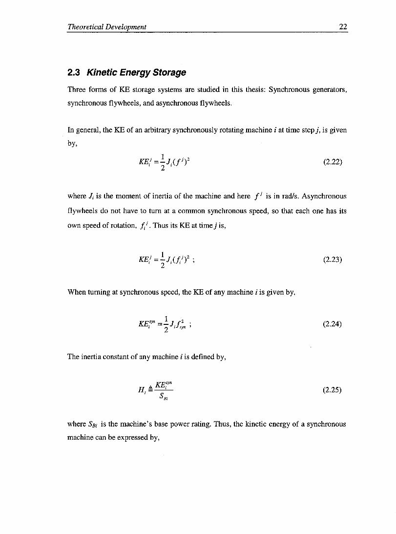
2.3 Kinetic Energy Storage
Three forms of KE storage systems are studied in this thesis: Synchronous generators,
synchronous flywheels, and asynchronous flywheels.
In general, the KE of an arbitrary synchronously rotating machine i at time step j, is given
by,
(2.22)
where Ji is the moment of inertia of the machine and here f j is in rad/s. Asynchronous
flywheels do not have to turn at a common synchronous speed, so that each one has its
own speed of rotation, h j • Thus its KE at time j is,
KEi = !J.( F.j)2 . 1 2 1 Ji '
When turning at synchronous speed, the KE of any machine i is given by,
KEsyn - 1 J f2 . i -Zisyn'
The inertia constant of any machine i is defined by,
KE~yn H.~--'-
1 SBi
(2.23)
(2.24)
(2.25)
where SEi is the machine's base power rating. Thus, the kinetic energy of a synchronous
machine can be expressed by,

Theoretical Development 23
(2.26)
while for an asynchronous flywheel, the KE in terms of the H constant is,
KEJ = .!..1.f2 (J/r = H.S (f/r 1 2 1 syn f2 1 BI f2
syn syn
(2.27)
The amount of KE stored at time step j can also be expressed in terms of the
corresponding frequency deviation. Thus, for a synchronous machine,
(2.28)
while for an asynchronous flywheel we have,
= KE?n (1 + L\f/ J2 !syn
(2.29)
As an example, for synchronous machines in standard power systems, assuming that the
maximum frequency deviation is ±600 mHz or ± 1 % of 60 Hz, then, from (2.26) the
maximum amount of KE exchange is approximately 2% of the KE stored in the rotating
masses at synchronous speed. For example, in a power system with 200 identical
synchronous machines each rated at 50 MV A with an H constant of 5s, the KE stored at
synchronous speed in each generator is HSB = 5x50 = 250 MI. Thus, the KE that can be
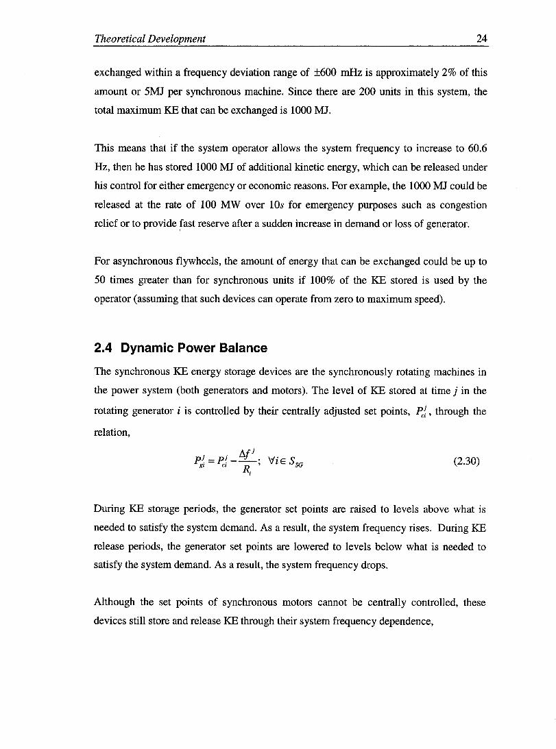
Theoretical Development 24
exchanged within a frequency deviation range of ±600 mHz is approximately 2% of this
amount or 5MJ per synchronous machine. Since there are 200 units in this system, the
total maximum KE that can be exchanged is 1000 MJ.
This means that if the system operator allows the system frequency to increase to 60.6
Hz, then he has stored 1000 MJ of additional kinetic energy, which can be released under
his control for either emergency or economic reasons. For example, the 1000 MI could be
released at the rate of 100 MW over lOs for emergency purposes such as congestion
relief or to provide fast reserve after a sudden increase in demand or loss of generator.
For asynchronous flywheels, the amount of energy that can be exchanged could be up to
50 times greater than for synchronous units if 100% of the KE stored is used by the
operator (assuming that such devices can operate from zero to maximum speed).
2.4 Dynamic Power Balance
The synchronous KE energy storage devices are the synchronously rotating machines in
the power system (both generators and motors). The level of KE stored at time j in the
rotating generator i is controlled by their centrally adjusted set points, p.:{, through the
relation,
. . Ilfj P l - pl . \-Il' E S gi - ci ---, v SG
Ri (2.30)
During KE storage periods, the generator set points are raised to levels above what is
needed to satisfy the system demand. As a result, the system frequency rises. During KE
release periods, the generator set points are lowered to levels below what is needed to
satisfy the system demand. As a result, the system frequency drops.
Although the set points of synchronous motors cannot be centrally controlled, these
devices still store and release KE through their system frequency dependence,

Theoretical Development 25
The dynamic power balance for synchronous generators, that is, Vi E SSG; Vj, is then,
KEi KEi-1 - (pi pi P( ~i)) i - i - gi - di - i Q r
=(p~ -/).fi _p~ _p(Ji)Jr CI R. dl I-
1
(2.31)
where,
and where each the frequency deviation must respect,
(2.32)
Synchronous flywheels behave like synchronous generators with frequency regulation
but without set points, that is,
. 1 . p~ = __ /).N.
gl R. ~ , 1
(2.33)
Thus, as defined by (2.33), since there is no controllable set point, the power generated or
consumed by a synchronous flywheel, Pj;, must follow the system frequency and cannot
be controlled other than by centrally controlling the system frequency.
The dynamic power balance for synchronous flywheels, that is, Vi E S SF; Vj , is then,

Theoretical Development 26
KE j KEj-l - (pj pj D(5:j)) i- i - gi-di-.ri!L r
= (- !lfj - pj - p'(Ôj)Jr R. dl I_
1
(2.34)
where,
KE/ = KE~yn (1 + !lf j J2 . II!. ' syn
In addition, each synchronous flywheel has limits on the frequency deviation, that is,
(2.35)
Asynchronous flywheels behave like synchronous generators in that they also have
frequency regulation without set points. Rowever, each asynchronous flywheel, unlike
synchronous machines, has its own rotating speed, which can be controlled centrally by
the system operator (SQ). Since the speed can be controlled, the speed regulation droop-
~ . term, --, is not present. Renee, for asynchronous flywheels, p~ = 0 .
R
The only power that can be injected into or extracted from an asynchronous flywheel is
due to a change in speed (or KE). The dynamic power balance for asynchronous
flywheels, that is, Vi E S AF; Vj , is then,
KEj KEj-l -(pj pj D(5:j))
i - i - gi - di -.ri!L T
= (-Pi - ~(§/))T (2.36)
where,
In addition, each asynchronous flywheel has limits on the frequency deviation, that is,

Theoretical Development 27
Af'.min < A.(j < A.(max. \.-1' S UJ i - UJ i - UJ i ' v l E AF (2.37)
Because of these limits, if the KE of a rotating machine reaches its upper (lower) limit,
then it cannot absorb (release) any more energy.
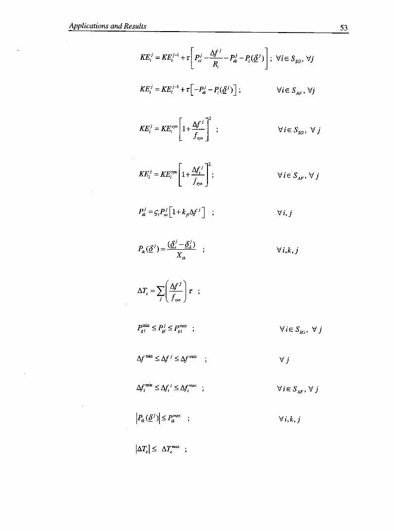
2.5 Generation Dispatch with Kinetic Energy Storage
Generation dispatch with KE storage tries to take advantage of the potential to store or
release energy in order to find a better feasible dispatch. The objective function can be to
minimize the total production cost over aIl generators over the entire time horizon taking
into account the KE storage capabilities of all rotating machines. From the previous
sections, mathematically this takes the form,
nt
Objective Function: C = L L Ci(pj;)T j=l ieSSG
subject to,
Generator Model: . . 1 .
p~ = p~ __ ~f'l • g. c, R. ~ ,
•
LoadModel: Vi,j
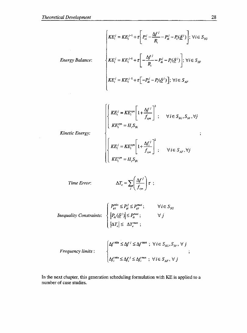
Theoretical Development
Energy Balance:
Kinetic Energy:
Time Error:
Inequality Constraints:
Frequency limits :
KEi -KEi-l [Pi /).fi pi D(J:i)]. \-1. S i - i +T ci -~- di -ri ~ ,viE SG
KEi - KEi-1 [/).f i pj P ( J: j)]. \-1. S i - i + T -~ - di - i ~ ,v 1 E SF
/).I: = ~(/).fj J T ; J fsyn
Pmin < pj < pmax. gi - gi - gi '
l~k(Qj)1 ~~;ax;
!/).I:! ~ /).I:max;
Vj
{
/).fmin ~/).fi ~/).fmax ; ViE SSG ' SSF' V j
/)./; min ~ /).f/ ~ /)./; max ; ViE S AF' V j
In the next chapter, this generation scheduling fonnulation with KE is applied to a number of case studies.
28
Applications and Results 29
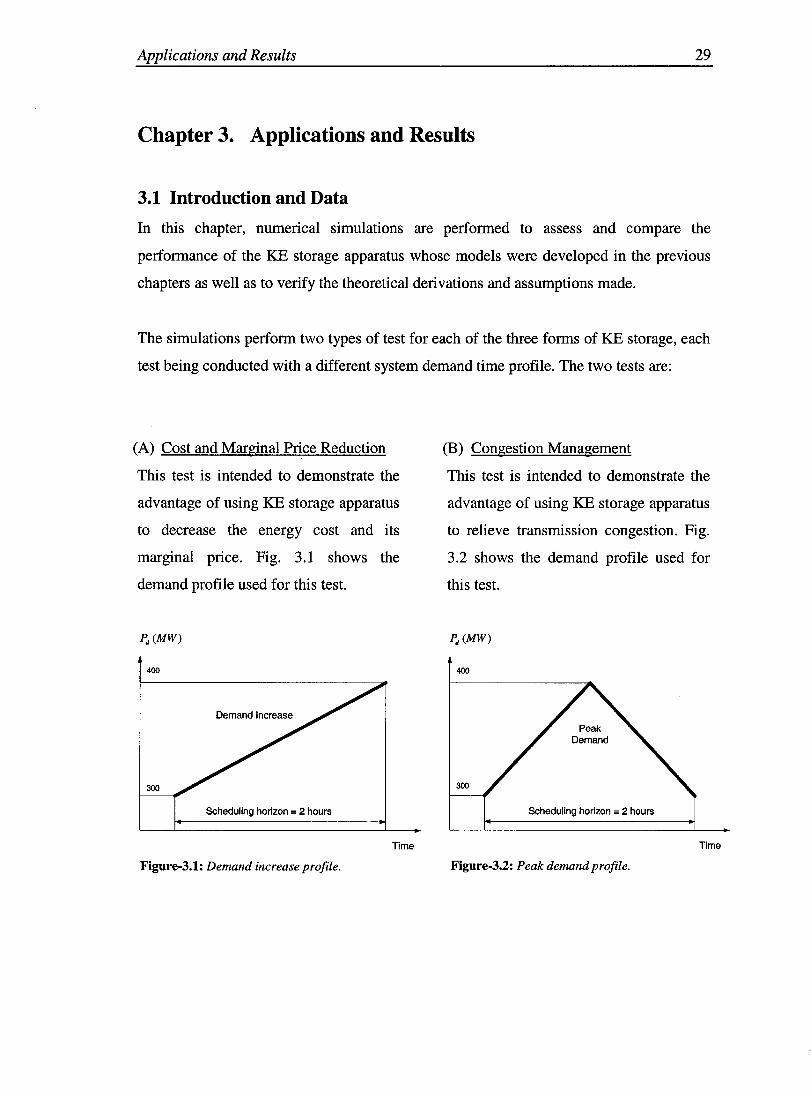
Chapter 3. Applications and Results
3.1 Introduction and Data
In this chapter, numerical simulations are performed to assess and compare the
performance of the KE storage apparatus whose models were developed in the previous
chapters as weIl as to verify the theoretical derivations and assumptions made.
The simulations perform two types of test for each of the three forms of KE storage, each
test being conducted with a different system demand time profile. The two tests are:
(A) Cost and Marginal Price Reduction
This test is intended to demonstrate the
advantage of using KE storage apparatus
to decrease the energy cost and its
marginal price. Fig. 3.1 shows the
demand profile used for this test.
~(MW)
400
300
Scheduling horizon = 2 hours
Time
Figure-3.1: Demand increase profile.
(B) Congestion Management
This test is intended to demonstrate the
advantage of using KE storage apparatus
to relieve transmission congestion. Fig.
3.2 shows the demand profile used for
this test.
400
300
Scheduling horizon = 2 hours
Time
Figure-3.2: Peak demand profile.

Applications and Results 30
In aIl simulations, the optimal scheduling problem is to minimize a co st function subject
to inequality and equality constraints as described in the previous chapter. The
mathematical software platform used for aIl simulations is GAMS (General Aigebraic
Modeling System) [19], which is suitable for solving large mathematical programming
problems.
The following is the set of the common data used in all simulations:
Table 3.1: Basic Data
Table 3.2: Bus Data
Table 3.3: Line Data

Applications and Results 31
3.2 KE Storage in Synchronous Generators
The three-bus system shown in Fig. 3.3 is used to perform the simulations over a
scheduling period of 2 hours with 5-minute time steps.
~~~----------------~----------------~~~
Figure-3.3: Three-bus system with generators and loads.
3.2.1 Generation Scheduling Formulation without Flywheels
According to the formulation of the previous chapter, the generation scheduling problem
without flywheels can be expressed in the following form:
min{c= t.I TC; (P/;)} }=lrESSG
where,
Vi,j
Subject to,
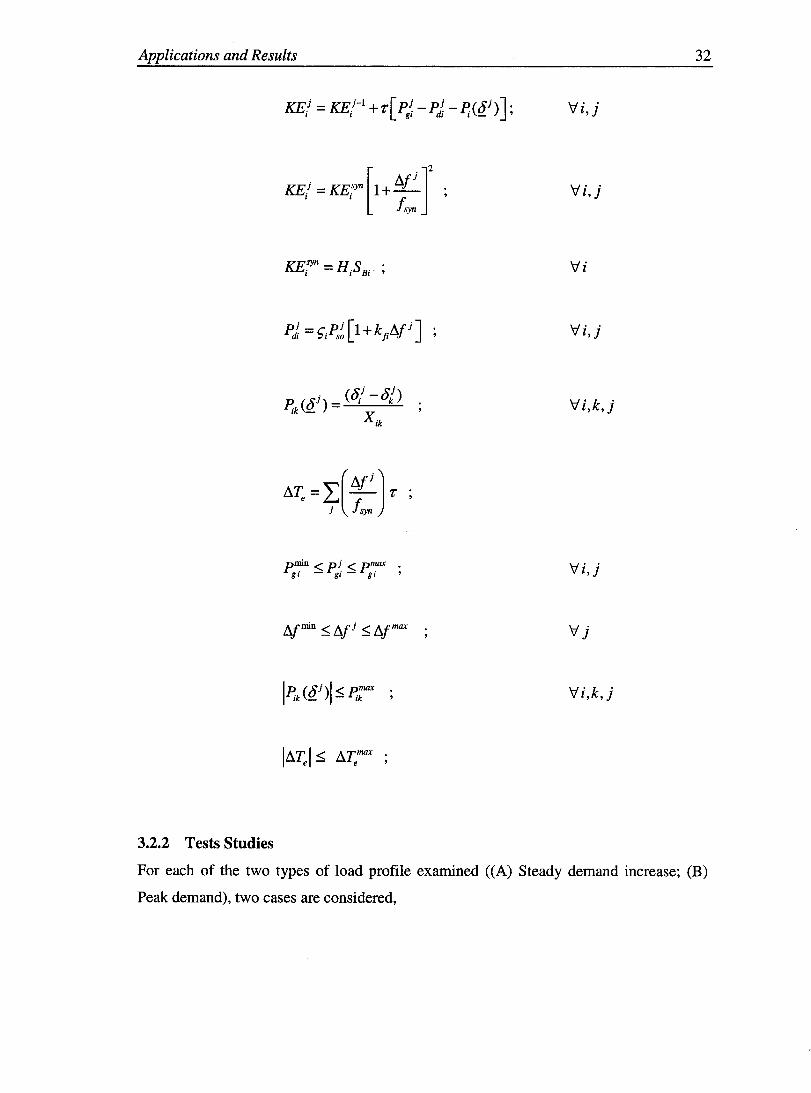
Applications and Results
3.2.2 Tests Studies
KE/ = KEt1 + r[ P~ - p); - P;(~/) J;
KE/ = KE/yn [1 + 111 j ]2 fsyn
P (8 j ) = (8/ - 8/) Ik - X
ik
Pmin < pj < p max gi - gi - gi
32
\;;fi,j
\;;fi, j
\;;fi
\;;fi, j
\;;fi,k,j
\;;fi, j
\;;fi,k,j
For each of the two types of load profile examined «A) Steady demand increase; (B)
Peak demand), two cases are considered,

Applications and Results 33
1) No system frequency variation (that is, no KE storage);
II) Frequency variation allowed within ±0.5Hz (with KE storage).
Test (A) Steady demand increase
Here, we focus on the impact of KE storage on cost and marginal cost reduction.
Difference in Costs (With and without KE storage):
The difference in costs is trivially small due to the small amount of KE that can be stored
and released in the synchronously rotating machines (three generators) for the narrow
frequency deviation allowed of ±0.5 Hz .
Table 3.4 shows the power defI1and, power generation as weIl as the power derived from
KE exchanges with the generators throughout the scheduled 24 time steps. It is seen that
at sorne time steps, sorne KE is absorbed or released. In the Table, three symbols for
power are used:
• pJ -represents the demand
• p~ - represents the power of generation
• pkGi represents the power derived over one time step from the KE exchange with
the generator, that is, I:!.KEbi _ - KEbi + KEb~l . ----""'-- ,
T T

Applications and Results 34
Table 3.4: Demand, generator power and power derived from the KE of synchronous generators. Test A,
Case Il: With KE storage.
The results of the power derived from the KE of the generators in Table 3.4 are shown
graphically in Fig. 3.4.

Applications and Results 35
Figure-3.4: Power from KE of synchronous generators. Test A, Case II: With KE storage.
Fig. 3.5 shows the prices over the scheduling horizon for both cases (Case I, without
frequency deviation, and Case II with frequency deviation). The prices at aIl buses are the
same as there is no line congestion.
Figure-3.5: System incremental cost (Priee) variation over time. Test A, Cases 1 and II: Without and with
KE storage in synchronous generators only.

Applications and Results 36
Table 3.5 shows the differenee in the priees between the two cases which is very small as
the KE storage in the synchronous generators of the system is not sufficiently large.
Table-3.5: System ineremental eosts (Priees) variation over time. Test A, Cases 1 and Il: Without and with
KE storage in synehronous generators only.
Test (B) Peak demand
Here, we focus on the impact of using the KE storage in the generators to relieve
congestion management. For this purpose, the line connecting buses 1 and 3 in the power
network is limited to 102 MW.
Table 3.6 shows the demand, power generation, as weIl as the power derived from KE
exchanges with generators during the scheduling period. It is seen that KE energy is

Applications and Results 37
stored during low demand periods to be released during high demand periods, when the
transmission line is congested.
Table 3.6: Demand, generator power, and power derived from the KE of synchronous generators. Test B,
Case II: With KE storage.
The results of Table 3.6 are shown graphically in Fig. 3.6.

Applications and Results 38
Figure-3.6: Power from KE of synehronous generators. Test B, Case II: With KE storage.
Fig. 3.7 shows that the single system price diverges into three different nodal prices
during congestion. This Figure applies for both cases 1 and II. So again, as in Test A, the
KE stored only in the rotating masses of the generators is not enough to have a sufficient
influence to relieve congestion and unify the le in all buses. This explains why the case
with and without frequency variation are essentially the same.
~,2,3 for both cases 1 & II
Figure-3.7: System and bus ineremental eosts (Priees) variation over time. Test B, Cases 1 and II: Without
and with KE storage in synehronous generators only.

Applications and Results 39
Table 3.7 shows the very small differences in the prices between cases 1 and II because of
the small amount of KE available from the synchronous generators.
Table-3.7: System and bus ineremental eosts (Priees) variation over time, Test B, Cases 1 and Il: Without
and with KE storage in synehronous generators only.
Table 3.8 shows the power flow variations over the 24 time-steps for the two case
studies. The Table shows that the small amount of KE storage in the synchronous
generators of the system is not sufficient to relieve the congestion of line 1-3 at 102 MW
at the peak of demand.
Applications and Results 40
Table-3.8: Power flow variation over time. Test B, Cases 1 and Il: Without and with KE storage in
synchronous generators only.
3.2.3 Case Comparisons and Conclusions
It can be seen from the tests summarized in Figs. 3.4 and 3.6 that the stored KE in the
rotating masses of the existing machines in a typical power system is not sufficient to
have a significant impact on power system economic or security operational objectives.
There is no significant gain in the cost and marginal cost as shown in Fig. 3.5, Tables 3.5
and 3.6. In addition, Fig. 3.8, Tables 3.7 and 3.8 show the insufficiency. of the stored KE
in synchronous generators to relieve congestion.

Applications and Results 41
Thus, in order to demonstrate the capability of KE storage within a synchronous system
to have a significant effect on power system economics and security, we now consider a
system with a large number of rotating synchronous flywheels.
3.3 KE Storage in Synchronous Flywheels
Synchronous flywheels are synchronous machines operating at the system frequency and
subject to the same narrow range of frequency variation as synchronous generators.
~2
~2
~3
Figure-3.8: Three bus system with generators, loads and synchronous flywheels.
3.3.1 Generation Scheduling Formulation with Synchronous Flywheels
According to the formulation of the previous chapter, the scheduling problem with
synchronous flywheels can be expressed in the following form:
where,
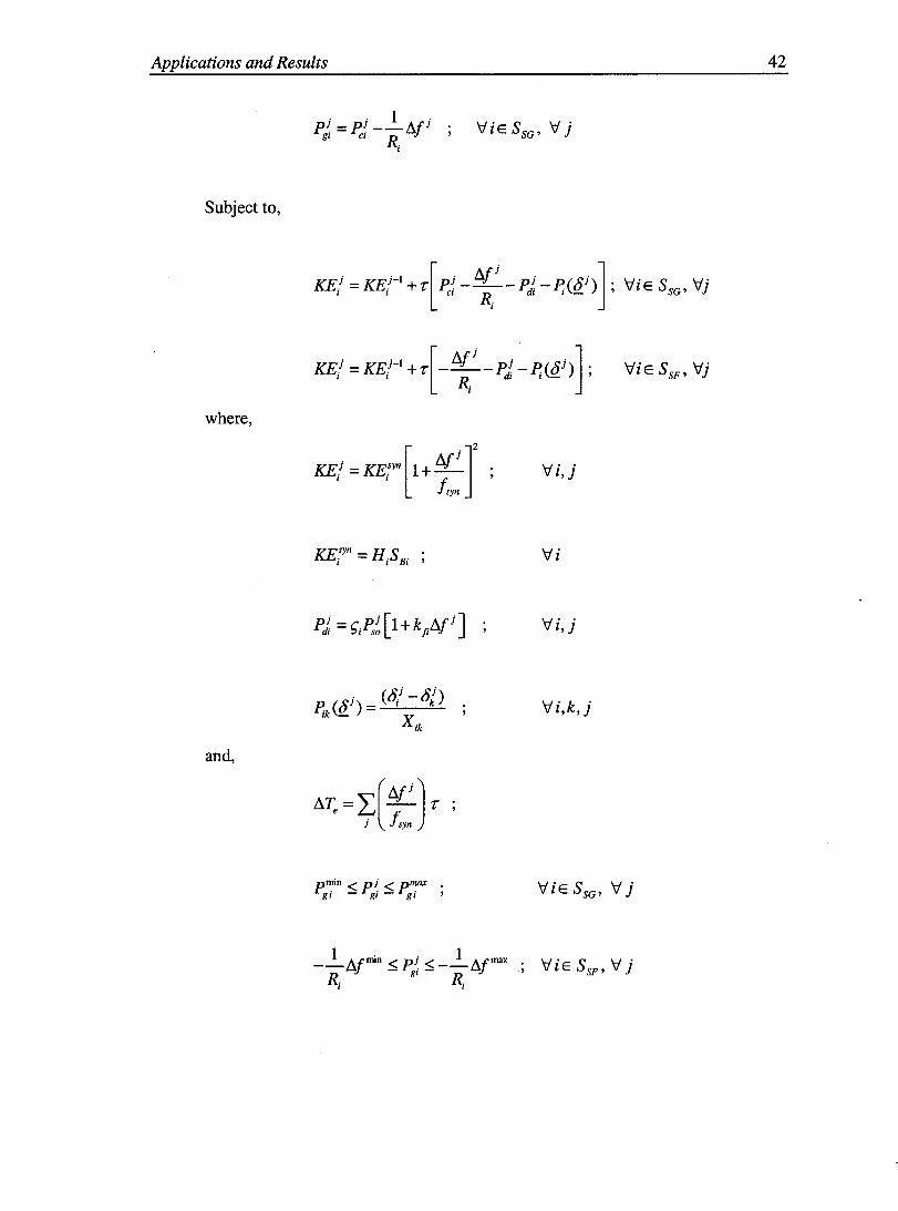
Applications and Results 42
p~ = p{ _J....,t!,/i gl CI R. ~
1
Subject to,
KEi - KEi-1 [Pi /::"fi pi P.(~i)], \-l' S \-l' i - i +1" ci -~- di - i Q ,vlE SG' v]
KEf = KEf-1 +1"[- /::"fi _pi - P'(8i)] , 1 1 R. dl 1 - ,
1
where,
KE/ = KE?n [1 + /::"f i ]2 fsyn
Vi,j
Vi
Vi,j
P. (8i ) = (8/ -81) Ik - X
ik
Vi,k,j
and,
P min < pi < pmax \-1 'E S \-1' gi - gi - gi V l SG' v]
_ J.... "t' min _< Pg]," _< _ J.... "t' max \-1 'E S \-l' u,J u,J vl SF'v] Ri Ri

Applications and Results 43
'Vj
'Vi,k, j
3.3.2 Tests Studies
Again, for each of the two tests examined «A) Steady demand increase; (B) Peak
demand), two cases are considered,
1) No system frequency variation (that is, no KE storage);
II) Frequency variation allowed within tO.5Hz (with KE storage).
This system contains the same generator and load data as in Section 3.2, however we
have added synchronous flywheel capability to bus 3, as seen in Fig. 3.8. One thousand
synchronous flywheels (m = 1000), each rated at 1000 MW s at 60 Hz, are installed in bus
3. The economics of adding synchronous flywheels are not considered at this time, the
goal being to demonstrate the capability of storing and exchanging sufficient KE in these
devices to have a significant impact on system economics and security.
Test (A) Steady demand increase
Here, we focus on the impact of KE storage on cost and marginal cost reduction.
Costs Difference with and without KE storage:

Applications and Results
From the above table, we see that with the installed synehronous flywheels, the overall
system hourly eost is improved by about 1 % when KE exehanges are used in the
generation seheduling.
44
Table 3.9 shows the demand, power generation as weIl as the power derived from KE
exehanges of synehronous generators and flywheels during the seheduling period. The
symbol plEsFi represents the power derived from the KE of synehronous flywheel i at
time step j, that is, I1KEfFi _ - KEf Fi + KEf;i' . ----"''-'- - ,
l' l'
The Table clearly demonstrates that the optimum generation sehedule stores KE during
low demand periods at lower priees to be released during high demand periods at higher
priees. This seheduling behavior is logieal.

Applications and Results 45
Table 3.9: Demand, generator power and power derived from the KE of synchronous generators and
flywheels. Test A, Case II: With KE storage.
Fig. 3.9 shows graphically the power exchange with the KE stored in the synchronous
flywheels. The power exchange with the KE stored in the generators is also shown in the
Figure, but it is extremely small compared to the power derived from the flywheels' KE.
Applications and Results 46
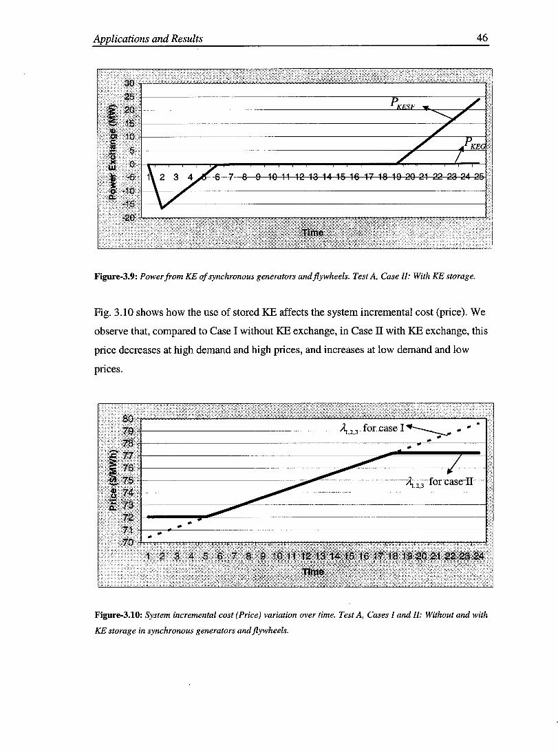
Figure-3.9: Power from KE of synehronous generators and flywheels. Test A, Case II: With KE storage.
Fig. 3.10 shows how the use of stored KE affects the system incremental cost (priee). We
observe that, compared to Case 1 without KE exchange, in Case II with KE exchange, this
priee decreases at high demand and high priees, and increases at low demand and low
priees.
Figure-3.10: System incremental eost (Priee) variation over time. Test A, Cases 1 and II: Without and with
KE storage in synehronous generators andflywheels.

Applications and Results 47
Test (H) Peak demand
Here, we focus on the impact of KE storage on congestion management.
Table 3.9 shows the demand, power generation as weIl as the power derived from KE
exchanges of synchronous generators and flywheels during the scheduling time period.
Again, it is seen that KE energy is stored during low demand periods at the beginning of
the scheduling horizon, to be released during the peak demand periods in the middle of
the scheduling horizon, thus relieving transmission line congestion.
Table 3.10: Demand, generator power and power derived from the KE of synchronous generators and
flywheels. Test B, Case II: With KE storage.
Fig. 3.11 shows graphically the power exchanges with the KE in the rotating masses of
synchronous generators and flywheels.

Applications and Results 48
Figure 3.11: Power from KE of synehronous generators and flywheels. Test B, Case II: With KE storage.
Fig. 3.12 shows that, when there is no KE exchange, the single system price splits into
three different nodal prices during the period of transmission congestion. In the case with
KE storage and exchange, there is a single system price over the entire horizon. This
means that the KE stored in the rotating masses of the synchronous flywheels is sufficient
to relieve congestion.
Figure-3.I2: System and bus incremental eosts (Priees) variation over time. Test B, Cases 1 and II:
Without and with KE storage in synehronous generators andflywheels.

Applications and Results 49
Table 3.10 shows numericaIly the difference in priees between the two cases. We notice
that for case-I with no KE storage, the nodal priees differ during congestion. In case-II
with KE storage, the congestion is relieved and this is reflected by having the same
marginal priee at aIl buses. This is highlighted in time steps (11, 12 and 13).
Table-3.1I: System and bus ineremental eosts (Priees) variation over time. Test B, Cases 1 and Il: Without
and with KE storage in synehronous generators and flywheels.
Table 3.12 shows the power flow variations over the 24 time-steps for the two case
studies. The Table shows that in the first case without KE storage in the synchronous
generators and flywheels, there is congestion in transrriission line 1-3 at 109 MW. In the

Applications and Results 50
second case with KE storage in synchronous generators and flywheels, the congestion is
relieved.
Table-3.12: Power flow variation over time. Test B, Cases 1 and Il: Without and with KE storage in
synchronous generators and flywheels.
3.3.3 Case Comparisons and Conclusions
It has been seen from the tests that the amount of KE stored (106 MWs) in the
synchronous flywheels and the level of KE exchanged (2% of 106 MWs) with the
synchronous flywheels is now sufficient to have a significant influence on the security
and economics of the system.

Applications and Results 51
We observe in Fig. 3.9 that the power derived from the KE exchange is negative at the
beginning of the scheduling time horizon. This means that during this period in which the
demand and the prices of electricity are low, KE is being stored in the synchronous
generators and flywheels. At the end of the scheduling time horizon, the power derived
from the KE becomes positive, meaning that KE is being released at a time when the
demand and the price of electricity are high. In the case of peak demand, Fig. 3.11 shows
that KE is released in the middle of the scheduling horizon where the peak occurs. The
optimization decides the optimal time for storing and releasing KE. Comparing the costs
and incremental costs (prices) in Fig. 3.10, we conclude that the economic advantages of
using KE storage are significant compared to the case without KE storage. As weIl, Fig.
3.12 shows that the capability of the stored KE in the synchronous flywheels to relieve
congestion is significant.
This section has shown that it is possible to influence power system security and
economics through KE storage in synchronous flywheels. However, to achieve the 106
MWs of installed flywheel KE, we would need to install a large number of synchronous
machines who se cost may be prohibitive. We therefore now consider the installation of
asynchronous flywheels having a broad range of rotational speed instead of the 2%
possible with synchronous machines.

Applications and Results 52
3.4 KE Storage in Asynchronous Flywheels
To study this alternative, an asynchronous flywheel as an ESA is installed at bus 3 of the
3-bus system shown in Fig. 3.13.
~2
~1
Et3 ~3
~3
Figure-3.13: Three bus system with generators, loads and asynchronous flywheel
3.4.1 Generation Scheduling Formulation with Asynchronous Flywheels
Based on the modeling and fonnulation presented in the previous sections, the scheduling
problem with asynchronous flywheels can be expressed in the following fonn:
min{c= f.I t'Cj(P~)} J=l IESSG
where,
Subject to,
Applications and Results 53
KE j KEj-l [pj /!:;.f j pj D ( ~ j)]. \-1. S \-1 • i = i + r ci - ~ - di -.ri!!. ,v l E SG' v]
KE/ = KE/yn [1 + /!:;.f j ]2 fsyn
Vi,j
Vi,k,j
Pmin < pj < pmax gi - gi - gi
Vj
Vi,k,j

Applications and Results 54
3.4.2 Tests Studies
The comparison for asynchronous flywheels application in both tests is done between two
cases:
I) Without asynchronous flywheel;
II) With asynchronous flywheel.
Again, this system contains the same generator and load data as in the previous sections;
however as seen in Fig. 3.13, at bus 3 we have added an asynchronous flywheel rated at
speeds varying between 0 Hz and 1651 Hz, and corresponding levels of stored KE
between 0 and O.6x 106 MWs.
The goal here is to demonstrate the capability of storing and exchanging sufficient KE in
this asynchronous device to have a significant impact on system economics and security.
In the tests that follow, the initial speed and KE of the flywheel at the beginning of the
scheduling period is assumed to be zero.
Test (A) Steady demand increase
Here, we focus on the impact of KE storage on cost and marginal cost reduction.
Costs difference for case-I without asynchronous flywheel and case-II with asynchronous
flywheel:
Table 3.13 shows the demand, power generation as well as the power derived from KE
exchanges with the asynchronous flywheel and synchronous generators during the
scheduling period. It is seen how KE energy is stored during low demand periods to be

Applications and Results 55
released during high demand periods. We have defined P!œAF as the power derived from
A VE j KE j KE j - 1 L.l.ft. AFi _ - AFi + AFi -_:..:...:... the KE exchange of the asynchronous flywheel, that is,
Table 3.13: Demand, generator power and power derived from the KE of synchronous generators and
asynchronous flywheel. Test A, Case II: With asynchronous flywheel.
Fig. 3.14 shows graphically the power exchange with the KE stored in the asynchronous
flywheel, as weIl as the power exchange with the KE stored in generators, which is
extremely small compared to the amount from the asynchronous flywheel.

Applications and Results 56
Figure-3.14: Power !rom KE of synehronous generators and asynehronous flywheel. Test A, Case II: With
asynehronous flywheel.
Fig. 3.15 shows how the use of stored KE affects the system ineremental eost (priee). We
observe that, eompared to Case 1 without KE exehange, in Case TI with KE exehange, this
priee deereases at high demand and high priees, and inereases at low demand and low
priees.
Figure-3.15: System ineremental eost (Priee) variation over time. Test A, Cases 1 and II: Without and with
asynehronous flywheel. KE storage in synehronous generators and asynehronous flywheel.

Applications and Results 57
Test (B) Peak demand
Here, we focus on the impact of KE storage on congestion management.
Table 3.14 shows the demand, power generation as weIl as the power derived from KE
exchanges of synchronous generators and asynchronous flywheel during the scheduling
time horizon. Again, it is seen that KE energy is stored during low demand periods at the
beginning of the scheduling horizon, to be released during the peak demand periods in
the middle of the scheduling horizon, thus relieving transmission line congestion.
Table 3.14: Demand, generator power and power derived from the KE of synchronous generators and
asynchronous flywheel. Test B, Case II: With asynchronous flywheel.

Applications and Results 58
Fig. 3.16 shows graphically the variation of power exchanges with the KE stored and
released in the rotating mass of the asynchronous flywheel and synchronous generators.
Figure 3.16: Power from KE of synchronous generators and asynchronous flywheel. Test B, Case Il: With
asynchronous flywheel.
Fig. 3.17 shows that, when there is no KE exchange with the asynchronous flywheel, the
single system price splits into three different nodal priees during the period of
transmission congestion. In the case with KE storage and exchange with the
asynchronous flywheel, there is a single system price over the entire horizon. This means
that the KE stored in the rotating masses of the asynchronous flywheel is sufficient to
relieve congestion.

Applications and Results 59
~,2,3 for case 1
Figure-3.17: System and bus incremental costs(Prices) variation over time. Test B, Cases 1 and II: Without
and with asynchronous flywheel. KE storage in synchronous generators and asynchronous flywheel.
Table 3.15 shows numericaIly the difference in prices between the two cases. We notice
that for case-I with no KE storage in the asynchronous flywheel, the nodal prices differ
during congestion. In case-II with KE storage in the asynchronous flywheel, the
congestion is relieved and this is reflected by having the same price at aIl buses. This is
highlighted in time steps (11, 12 and 13).

Applications and Results 60
Table-3.15: System and bus ineremental eosts (Priees) variation over time. Test B, Cases 1 and II: Without
and with asynehronous flywheel. KE storage in synehronous generators and asynehronous flywheel
Table 3.16 shows the power flow variations over the 24 time-steps for the two case
studies. The Table shows that in the first case without KE storage in asynchronous
flywheel, there is congestion in the transmission line 1-3 at 109 MW. In the second case
with KE storage in asynchronous flywheel, the congestion is relieved.

Applications and Results 61
Table-3.16: Power flow variation over time. Test B, Cases 1 and II: Without and with asynchronous
flywheel. KE storage in synchronous generators and asynchronous flywheel.
3.4.3 Case Comparisons and Conclusions
We conc1ude from the tests that the specified amount of KE storage in the asynchronous
flywheel is sufficient to meet the eeonornic and security goals.
Again, with the KE stored in and exchanged with the asynehronous flywheel, we
observed in Fig. 3.14 that the power derived from the KE exchange is negative at the
beginning of the seheduling time horizon, identifying this as a period of KE storage that
takes advantage of the low priees under low demand. During the last few time steps of
the scheduling horizon, the power derived from the KE becomes positive, meaning that

Applications and Results 62
KE is released to take advantage of the high priees during the period of high demand. Fig.
3.16 leads to a similar observation, but here the release of KE happens in the middle of
the scheduling horizon to coincide with the peak demand. In aIl cases, the optimization
method decides when to store and release KE in order to minimize the overall co st.
The difference between asynchronous and synchronous flywheels is that the former can
store much more KE in accordance with its much wider range of frequency variation, and
fewer such devices would be needed compared to the case with synchronous flywheels.
3.5 KE Storage and Exchange for Emergency Fast Reserve
Applications
Another application of the use of KE storage is as a source of fast reserve in case of a
contingency where a generator is tripped off. Typically, what happens then is that the
frequency deviation, 11/, begins to drop, causing the primary regulation in the healthy
units to increase their output.
Security requirements dictate that in the event of losing any single generator, the
frequency deviation should not exceed a specified limit, e.g. 0.5 Hz. Assuming that
network congestion is not active, the power balance before the loss of a generator must
satisfy,
(3.1)
where Pgi is the set point of generator i. We assume that at these set points, the system
frequency is at its normallevel, or equivalently that the frequency deviation, 11/ = 0 .
After the loss of generator 1, the primary regulation is activated, and if the system is
stable, without KE storage and exchange, after about 10 seconds, the system settles to a
new steady-state given by,

Applications and Results 63
(3.2)
where Ilfz is the frequency deviation from normal about 10 seconds after the loss of
generator l.
Thus, security requires that for aIl l, Illfz 1 ~ Ilfmax (3.3)
With KE storage and exchange, after the loss of generator l, again, after about 10
seconds, the system settles to a new steady-state given by,
(3.4)
where 1" = 10 sand,
(3.5)
and where,
(3.6)
But, since the frequency deviation is smaIl,
IlKE. :::: 2KE~yn Ilfz , 'f. syn
(3.7)
Substituting (3.7) into (3.4) and rearranging gives,
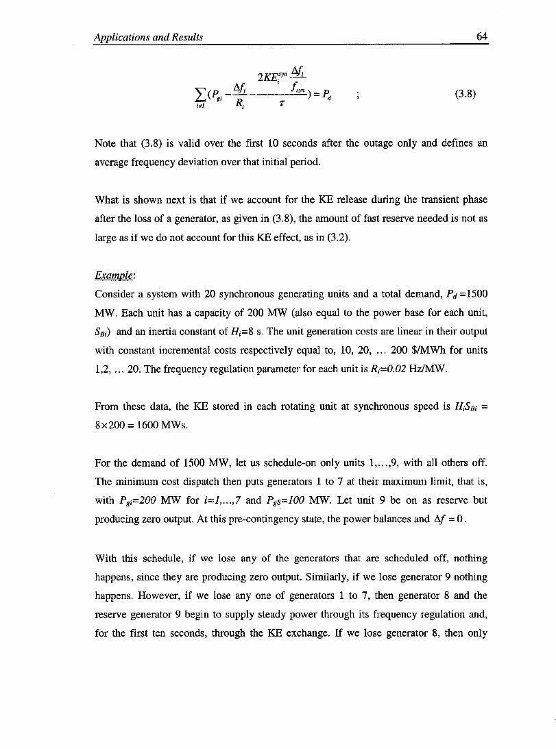
Applications and Results 64
(3.8)
Note that (3.8) is valid over the first 10 seconds after the outage only and defines an
average frequency deviation over that initial period.
What is shown next is that if we account for the KE release during the transient phase
after the loss of a generator, as given in (3.8), the amount of fast reserve needed is not as
large as if we do not account for this KE effect, as in (3.2).
Example:
Consider a system with 20 synchronous generating units and a total demand, Pd =1500
MW. Each unit has a capacity of 200 MW (also equal to the power base for each unit,
SBi) and an inertia constant of Hi=8 s. The unit generation costs are linear in their output
with constant incremental costs respectively equal to, 10, 20, ... 200 $lMWh for units
1,2, ... 20. The frequency regulation parameter for each unit is Ri=O.02 HzIMW.
From these data, the KE stored in each rotating unit at synchronous speed is HiSBi =
8x200 = 1600 MWs.
For the demand of 1500 MW, let us schedule-on only units 1, ... ,9, with aH others off.
The minimum co st dispatch then puts generators 1 to 7 at their maximum limit, that is,
with Pgi=200 MW for i=1, ... ,7 and Pg8=100 MW. Let unit 9 be on as reserve but
producing zero output. At this pre-contingency state, the power balances and !!:..f = 0 .
With this schedule, if we lose any of the generators that are scheduled off, nothing
happens, since they are producing zero output. Similarly, if we lose generator 9 nothing
happens. However, if we lose any one of generators 1 to 7, then generator 8 and the
reserve generator 9 begin to supply steady power through its frequency regulation and,
for the first ten seconds, through the KE exchange. If we lose generator 8, then only

Applications and Results 65
generator 9 will provide power through its frequency regulation. However, in aIl cases,
for the first 10 seconds aIl generators will supply power from KE exchange.
The logical assumption is that the secondary and tertiary generation control is too slow to
act during the first 10 seconds, during which time aIl generation set points remain
constant.
Thus, if we allow the frequency to drop by its maximum 0.5 Hz, the power that can be
extracted from the KE stored in each of the scheduled-on generators, within the transient
phase of 10 s, is,
2(8x200) 0.5 = ____ 6~0~
lOs
3200 0.5 = _----.:::6~0 = 26.67 MW for 10 s
lOs
In our case, we have nine generators scheduled-on, so that after losing one, we can
extract eight times this KE, that is,
LPKEi =26.67x8=213.36MW for lOs (3.9) i=8
To this amount of generating power extracted from the KE, we can add the regulation
components provided by generator 9 and possibly by generator 8 (if 8 is not the one lost),
since these two generators operate below their maximum of 200 MW. If the frequency is

Applications and Results 66
allowed to drop by 0.5 Hz, the regulation terms provided by generators 8 and 9 could be
_ !:::.f = _ -0.5 = 25 MW . Ri 0.02
From (3.9), we can conclude that with 8 scheduled on generators and one reserve, after
the loss of any single generator, there is enough power available in the KE of the
remaining rotating masses to balance the load over the first ten seconds. In fact, if we also
consider the 25 MW of regulating power from the reserve generator, we would have
enough fast reserve by scheduling 7 generators with one reserve.
What is important, is that if our model does not consider KE exchange over the first ten
seconds, then we would have to schedule 7 more reserve generators producing zero
output to be able to supply the necessary power from the regulating components only.
We emphasize that the power from KE exchange is only temporary, that is, it is available
only during the transient (about ten seconds) following a contingency. Thus, it is
necessary for the secondary control to begin to increase the set point after this transient
interval so that the power can continue to be balanced.

Conclusions and Recommendations 67
Chapter 4: Conclusions and Recommendations
4.1 Conclusions
Kinetic energy (KE) storage systems have been analyzed as an energy storage technology
to be integrated into power system operation with the goal of reducing operational costs,
attenuating nodal price spikes, and relieving network congestion.
Two types of system demand variation (steady increase and peak demand) have been
examined to show the relative effectiveness of KE storage systems.
The motivation behind choosing this type of energy storage system was because power
systems have been traditionally equipped to be able to change the rotor speed of
generators providing an efficient, reliable mechanism for storing and withdrawing
energy. The normal use of the stored KE is to correct accumulated frequency deviations,
which manifests itself as a time error on electric clocks. The idea here however was to
deploy this naturally av ail able capability as a mechanism for releasinglabsorbing KE
to/from the power system.
This thesis shows that the av ail able amounts of KE storage in typical synchronous power
systems could be enough to provide fast reserve after events where short bursts of energy
are needed, such the sudden loss of a generator. In addition, this type of KE storage can
serve to perform time error correction. However, the amount of KE stored in the rotating
masses of generators and motors in a typical power system is not enough to reduce the
energy cost or to relieve network congestion in a significant way.
Synchronous flywheels were also considered in this thesis to investigate whether this
form of KE storage would be able to significantly influence system operation. This
investigation only looked at technical feasibility without accounting for the cost of
installing flywheels. The conclusions with respect to synchronous flywheels are the same
as those reached for synchronous machines. Essentially, the range of allowed frequency
Conclusions and Recommendations 68
deviation in a synchronous system, typically less than ± 0.5 Hz, is too small to permit the
storage and release of sufficient amounts of energy other than for short bursts lasting less
than 10 seconds. This is useful as a source of fast reserve, but it cannot produce steady
levels of power lasting for periods of around one hour, quantities that would be required
to have a significant impact on power system economics and security.
The use of asynchronous flywheels with a much broader range of frequency deviation is
more promising however. From the results of chapter-3, one can conclude that significant
overall co st reduction can be achieved by borrowing energy from the stored KE when the
prices are high and by restoring the KE when the prices are low. The results also show
that congestion management based on the optimum utilization of stored KE can relieve
transmission line congestion and attenuate nodal price volatility during peak demand
periods.
4.2 Recommendations
Future studies should examine both the technical potential and the costs of asynchronous
flywheels, including losses. There are two types of losses: 1) InternaI that take place
inside the flywheel due to friction of the masses rotating at a very high speed; 2) External
los ses that take place within power electronic energy conversion devices.
A technical and cost comparison could be done between asynchronous flywheels and
other types of energy storage technologies.
Operationally, one can view the use of stored kinetic energy as a distributed generation
system (DG) with the following characteristics:
• It is brought on line only when the energy priee exceeds a pre-set incremental
price cap;
• It can operate both in generating and motoring modes;
• It can be dispatched as a normal generator within its generation range, based on
the market-clearing mIes;

Conclusions and Recommendations 69
• The set point of this DG is realized directly by the AGC software at the control
centre, as opposed to being transmitted to the generators' power plants;
• The capacity of this DG is given by a frequency band, defined by the power utility
(or the market), around the standard system reference frequency;
Once the DG reaches its capacity limit (i.e. the maximum allowable frequency deviation),
it can no longer maintain the system incremental cost at the price cap. Nevertheless, it
would still be able to reduce the system incremental cost by supplying part of the
required generation. When the system incremental co st falls below the set incremental
price cap, the DG is turned off. At this time, one has to have an accurate amount of the
total energy supplied by the DG to the market.
A market-clearing program and an AGC program could be developed to simulate a
combination of load-frequency control (LFC) and energy market auction for an isolated
power system. The power system can be assumed to have a number of generating units,
sorne of which will be assigned priee curves that will be very expensive to operate around
their maximum generation range. The short-term system demand profile can be assumed
to be available and defined such that, in the absence of the DG, its peak values lead to
major price spikes. Also, to increase price instability, on a weekly basis, sorne generators
could be chosen at random to go on maintenance.
Finally, a future extension of this work is to analyze in more detail how to use stored KE
as a fast reserve in primary frequency regulation following the loss of a generating unit.

References 70
References
[1] Olle I. Eigerd, Electric Energy Systems Theory: An Introduction, 2nd Edition,
McGraw-Hill,lnc. 1971.
[2] J.D. Glover, M. Sarma, Power System Analysis and Design, 3rd Edition,
Brooks/Cole, 2002.
[3] James A. Momoh, Electric Power System Applications of Optimization, Marcel
Dekker, Inc. 2001.
[4] Arthur R. Bergen, Vijay Vittal, Power System Analysis, 2nd Edition, Prentice
Hall, Inc. 2000.
[5] Vineent Del Toro, Electric Power Systems, Prentice-Hall, Inc. 1992.
[6] N. Jaleeli, L.S. VanSlyck, D.N. Ewart, L.H. Fink, A.G. Hoffman, "Understanding
Automatic Generation Control", Transaction on Power Systems, Vol. 7, No. 3,
August 1992.
[7] Khadim Hussain, "Control Performance Analysis of Interconnected Power
Systems", IEEE Computer Application in Power, 1994.
[8] P.D. Henderson, H. Klaiman, J. Ginnetti, T. Snodgrass, N. Cohn, S. Bloor, L.
VanSlyck, "Co st Aspects of AGC, Inadvertent and Time Error" , IEEE
Transactions on Power Systems, Vol. 5, No. 1, February 1990.
[9] L. VanSyck, N. Jaleeli, W. Robert Kelley, "Implications of Frequency Control
Bias Settings on Interconnected System Operation and Inadvertent Energy
Accounting", IEEE Transactions on Power Systems, Vol. 4, No.2, May 1989.
[10] W.W. Priee, H. D. Chiang, H.K. Clark, D.C. Concordia, "Load Representation for
Dynamic Performance Analysis", IEEE Transactions on Power Systems, Vol. 8,
No. 2, May 1993.
[11] S. Banerjee, J.K. Chatterjee, S.c. Tripathy, "Application of Magnetic Energy
Storage Unit as Load-Frequency Stabilizer", IEEE Transactions on Energy
Conversion, Vol. 5, No. 1, March 1990.

References 71
[12] Susan M. Schoenung, Clay ton Burns, "Utility Energy Storage Applications
Studies", IEEE Transaction on Energy Conversion, Vol. 11, No. 3, September
1996.
[13] Z. Jiancheng, H. Lipei, Wu Su, "Research on Flywheel Energy Storage System
for Power Quality" IEEE 2002.
[14] Satoshi Uemura, Shinichi Nomura, Ryuichi Shimada, "Stabilization of Electric
Power System using the Variable Speed Flywheel Generator", IEEE 1997.
[15] Hans J. Bornemann, Michael Sander, "Conceptual System Design of a 5
MWh/100 MW Superconducting Flywheel Energy Storage Plant for Power
Utility Applications", IEEE Transactions on Applied Superconductivity, Vol. 7,
No. 2, June 1997.
[16] John D. Boyes, Nancy H. Clark, "Technologies for Energy Storage Flywheels and
Super Conducting Magnetic Energy Storage", Energy Storage Program-Sandia
National Laboratories, IEEE 2000.
[17] B. Bhargava, G. Dishaw, "Application of an Energy Source Power System
Stabilizer on the 10 MW Battery Energy Storage System at Chi no Substation",
IEEE Transaction on Power Systems, Vol. 13, No. 1, February 1998.
[18] Ph.G. Rutberg, R.B. Goncharenko, E.G. Kasharsky, "About Prospects of
Application of the Flywheel Stabilizer of Frequency in a Power System", Institute
of Problems of Electro physics of Russian Academy of Science" IEEE 2002.
[19] GAMS/CPLEX A User's Guide, GAMS Development Corporation, 2003.
[20] Margaret Toussaint, "An Analytical Study of the Load Flow Problem", Master
Thesis at McGill University, Montreal, Canada, September 1994.
[21] Ivana Kockar, "Iterative Generation of Synthetic Power System Networks for
Load Flow Studies", Master Thesis at McGill University, Montreal, Canada, July
1998.