This journal is© the Owner Societies 2016 Phys. Chem. Chem. Phys., 2016, 18, 28325--28338 | 28325

Cite this:Phys.Chem.Chem.Phys.,

2016, 18, 28325

Application of classical simulations for thecomputation of vibrational properties of freemolecules†

Denis S. Tikhonov,*ab Dmitry I. Sharapa,c Jan Schwabedissena andVladimir V. Rybkin*d

In this study, we investigate the ability of classical molecular dynamics (MD) and Monte-Carlo (MC)

simulations for modeling the intramolecular vibrational motion. These simulations were used to compute

thermally-averaged geometrical structures and infrared vibrational intensities for a benchmark set previously

studied by gas electron diffraction (GED): CS2, benzene, chloromethylthiocyanate, pyrazinamide and 9,12-I2-

1,2-closo-C2B10H10. The MD sampling of NVT ensembles was performed using chains of Nose–Hoover

thermostats (NH) as well as the generalized Langevin equation thermostat (GLE). The performance of the

theoretical models based on the classical MD and MC simulations was compared with the experimental data

and also with the alternative computational techniques: a conventional approach based on the Taylor

expansion of potential energy surface, path-integral MD and MD with quantum-thermal bath (QTB) based

on the generalized Langevin equation (GLE). A straightforward application of the classical simulations

resulted, as expected, in poor accuracy of the calculated observables due to the complete neglect of

quantum effects. However, the introduction of a posteriori quantum corrections significantly improved the

situation. The application of these corrections for MD simulations of the systems with large-amplitude

motions was demonstrated for chloromethylthiocyanate. The comparison of the theoretical vibrational

spectra has revealed that the GLE thermostat used in this work is not applicable for this purpose. On the

other hand, the NH chains yielded reasonably good results.

1 Introduction1.1 Geometrical and vibrational studies of free molecules

The studies of structural and vibrational properties of freemolecules in the ground state have been around in the scientificcommunity since the dawn of quantum chemistry and modernphysical methods.1–4 The value of such data is not exhausted bythe information relevant for a specific chemical application.

They have been used for many purposes in theoreticalchemistry.5,6 Notable examples are:� development of valence theory5,7 by Linus Pauling,� theoretical background and experimental support for the

valence shell electron pair repulsion theory (VSPER),6

� usage of experimental geometrical parameters of moleculesin the gas phase for parameterization of AM1 and MNDO semi-empirical models,8–10 and the functional MN15-L.11

Therefore, the experimental gas-phase molecular structurestudies should not be underestimated. The three main methodsfor investigation of the ground state geometrical or/and vibra-tional properties of free molecules are:� gas-phase electron diffraction (GED),7,12

� IR or Raman vibrational spectroscopy (VSp),4,13

� rotational spectroscopy (RSp).4,13

The interpretation can be done by solving either direct orinverse problems.14,15 In both cases a theoretical model isrequired. A direct problem is basically a simple comparisonof experimental data with that computed from the model.In this case, a theoretical model is usually based on quantumchemical calculations (QC). The inverse problem supposes thata theoretical model can be parametrized with a set of variables

a Universitat Bielefeld, Lehrstuhl fur Anorganische Chemie und Strukturchemie,

Universitatsstrasse 25, 33615, Bielefeld, Germany.

E-mail: denis.tikhonov@uni-bielefeld.deb M. V. Lomonosov Moscow State University, Department of Physical Chemistry,

GSP-1, 1-3 Leninskiye Gory, 119991 Moscow, Russiac Computer-Chemie-Centrum and Interdisciplinary Center for Molecular Materials,

Department Chemie und Pharmazie, Friedrich-Alexander-Universitat

Erlangen-Nurnberg, 91052 Erlangen, Germanyd ETH Zurich, Department of Materials, Wolfgang-Pauli-Strasse 27, CH-8093 Zurich,

Switzerland. E-mail: vladimir.rybkin@mat.ethz.ch

† Electronic supplementary information (ESI) available: UNEX input files thatwere used to perform the comparison of theoretical GED models with experi-mental data for BNZ, CMTC, PZA and ICB can be found. These files containcomputed re geometries and vibrational parameters (l, re–ra and 6�k) as well asexperimental sM(s) curves. See DOI: 10.1039/c6cp05849c

Received 24th August 2016,Accepted 9th September 2016

DOI: 10.1039/c6cp05849c

www.rsc.org/pccp

PCCP

PAPER

Publ

ishe

d on

15

Sept

embe

r 20

16. D

ownl

oade

d by

Uni

vers

itat E

rlan

gen

Nur

nber

g on

03/

01/2

018

10:2

3:09

.

View Article OnlineView Journal | View Issue

28326 | Phys. Chem. Chem. Phys., 2016, 18, 28325--28338 This journal is© the Owner Societies 2016

(e.g. geometrical parameters,16–24 the parametric form of potentialenergy for internal motions18,21,25 or some mean parameters suchas scale factors for harmonic force fields18,20,21). These experi-mental parameters are obtained by fitting the theoretical model tothe experimental data. Unfortunately, all the parameters of themodel can be unequivocally obtained from the experimental dataonly for small molecules, otherwise the inverse problem becomesill-defined.26 Therefore, in most cases some parameters should betaken as they are from the theoretical computations based mainlyon QC. Consequently, the accuracy of these parameters is crucial.Fortunately, the effects arising from the choice of the QC approxi-mation are significantly smaller than the experimental uncertaintiesand systematic errors of the theoretical models used for fitting. As aconsequence, computationally cheap QC approaches can be usedin particular to account for molecular vibrations without any lossof accuracy.27

1.2 Theoretical models for intramolecular vibrations

Let us assume the applicability of the Born–Oppenheimer (B–O)approximation. The direct solution of Schrodinger equationfor rovibrational levels on the preconstructed potential energysurface (PES) is possible only for small systems consisting of afew atoms.28–30 Therefore, for larger systems simplifications areintroduced. In cases of semi-rigid molecules, it is the separationof the rotational degrees of freedom, which are then treated as arigid rotor. A further simplification is the use of the harmonicoscillator approximation for the vibrations, giving rise to therigid rotor–harmonic oscillator (RR–HO) approximation.13,31,32

This model is a very reasonable zeroth approximation for themolecules with small-amplitude motion. All the leftover effects,i.e. vibration–rotation interaction and the higher-order (anharmonic)terms in Taylor expansion of PES can be introduced via perturbationtheory.4,15,19,33 In cases of non-rigid molecules the techniquedescribed above can be augmented by the direct treatment ofthe large-amplitude motion (LAM), for example, as it is describedin ref. 34. This model gives the observables for GED, VSp andRSp and also provides a framework for analysis and discussionof the experiments.

The anharmonic effects themselves are very important for thesuccessful interpretation of the experimental data.20,35–37 Thecubic force field is required for all the models (i.e. GED, VSp

and RSp). The quartic force field@4V

@qi@qj@qk@ql

� �is not that

necessary for GED and RSp since the main aharmonic shift ofthe atoms from the equilibrium position appears mainly due tothe cubic force field.19,38 In the case of VSp, the quartic forcefield appears in the first order of perturbation theory only as

semidiagonal elements@4V

@Qi2@Qj

2

� �in normal coordinates Q.38

Thus, its computation takes the same order of time as thecomputation of the harmonic force field. In this work, we do notconsider complete quartic force fields.

The higher the order of the PES Taylor expansion term, themore computationally expensive it is. The number of cubicforce constants grows as O(N3) with the size of the system, thecost of each constant growth being dependent on the electronic

structure method and its implementation. Consequently, at onepoint it becomes cheaper to use alternative techniques to deter-mine the gas-phase structure, for example, classical ab initiomolecular dynamics (MD) or Monte-Carlo (MC) simulations.39–41

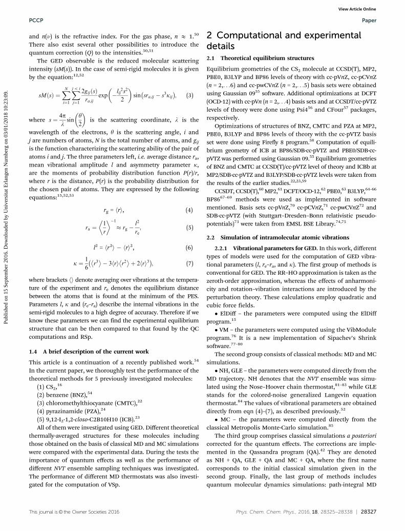
An estimate for the relation of times for performing MD simula-tions tMD to the computation of the cubic force field tCFF can bemade as follows:23,42

tMD

tCFF¼ a � b � nmax=nminð Þ

36N2; (1)

where nmax and nmin are the highest and the lowest vibrationalfrequencies for the chosen molecule, a shows how many timesteps are required to cover the period of the fastest vibrationand b shows how many periods of the lowest vibration arein the total length of the trajectory. Thus, a and b control thequality of the MD simulation. An illustration of this relationcan be found in Fig. 1.

In cases of non-rigid molecules with multiple LAMs a multi-dimensional PES scan along the LAM coordinates is required inaddition to a cubic force field. Therefore for such systems thecomputational cost of the conventional model grows even faster.

1.3 Application of classical simulations for gas electrondiffraction and vibrational spectroscopy

Classical ab initio MD simulations have been used to simulateVSp for quite a long time.46 The observable in a VSp experimentis the intensity (I) vs. the frequency (n). In the case of infraredabsorption, the theoretical spectrum from MD is calculated asfollows:47–49

IðnÞ / 1

nðnÞ n tanhhn

2kBT

� �|fflfflfflfflfflfflfflfflfflfflfflffl{zfflfflfflfflfflfflfflfflfflfflfflffl}

Q

Re

ð10

e�i2pnt dðtÞ; dð0Þh idt; (2)

where d is the electronic dipole moment of the system, hd(t),d(0)i = f (t) is the autocorrelation function of the dipole moment,

Fig. 1 Relative cost of MD simulation for the computation of the cubicforce field as approximated by eqn (1), a = 10 and b = 5. Triangles show thetheoretical behavior at nmax/nmin = 1000, circles demonstrate the applica-tion of this relation for some molecules that were recently investigatedusing GED.23,43–45

Paper PCCP

Publ

ishe

d on

15

Sept

embe

r 20

16. D

ownl

oade

d by

Uni

vers

itat E

rlan

gen

Nur

nber

g on

03/

01/2

018

10:2

3:09

. View Article Online

This journal is© the Owner Societies 2016 Phys. Chem. Chem. Phys., 2016, 18, 28325--28338 | 28327

and n(n) is the refractive index. For the gas phase, n E 1.50

There also exist several other possibilities to introduce thequantum correction (Q) to the intensities.50,51

The GED observable is the reduced molecular scatteringintensity (sM(s)). In the case of semi-rigid molecules it is givenby the equation:12,52

sMðsÞ ¼XNi¼1

Xjo i

j¼1

2gijðsÞra;ij

exp �lij2s2

2

� �sin sra;ij � s3kij� �

; (3)

where s ¼ 4plsin

y2

� �is the scattering coordinate, l is the

wavelength of the electrons, y is the scattering angle, i andj are numbers of atoms, N is the total number of atoms, and gij

is the function characterizing the scattering ability of the pair ofatoms i and j. The three parameters left, i.e. average distance ra,mean vibrational amplitude l and asymmetry parameter k,are the moments of probability distribution function P(r)/r,where r is the distance, P(r) is the probability distribution forthe chosen pair of atoms. They are expressed by the followingequations:15,52,53

rg = hri, (4)

ra ¼1

r

� ��1� rg �

l2

re; (5)

l2 = hr2i � hri2, (6)

k ¼ 1

6r3 � 3 rh i r2

þ 2 rh i3

� �; (7)

where brackets hi denote averaging over vibrations at the tempera-ture of the experiment and re denotes the equilibrium distancebetween the atoms that is found at the minimum of the PES.Parameters l, k and (re–ra) describe the internal vibrations in thesemi-rigid molecules to a high degree of accuracy. Therefore if weknow these parameters we can find the experimental equilibriumstructure that can be then compared to that found by the QCcomputations and RSp.

1.4 A brief description of the current work

This article is a continuation of a recently published work.54

In the current paper, we thoroughly test the performance of thetheoretical methods for 5 previously investigated molecules:

(1) CS2,16

(2) benzene (BNZ),54

(3) chloromethylthiocyanate (CMTC),22

(4) pyrazinamide (PZA),24

(5) 9,12-I2-1,2-closo-C2B10H10 (ICB).23

All of them were investigated using GED. Different theoreticalthermally-averaged structures for these molecules includingthose obtained on the basis of classical MD and MC simulationswere compared with the experimental data. During the tests theimportance of quantum effects as well as the performance ofdifferent NVT ensemble sampling techniques was investigated.The performance of different MD thermostats was also investi-gated for the computation of VSp.

2 Computational and experimentaldetails2.1 Theoretical equilibrium structures

Equilibrium geometries of the CS2 molecule at CCSD(T), MP2,PBE0, B3LYP and BP86 levels of theory with cc-pVnZ, cc-pCVnZ(n = 2,. . .6) and cc-pwCVnZ (n = 2,. . .5) basis sets were obtainedusing Gaussian 0955 software. Additional optimizations at DCFT(OCD-12) with cc-pVn (n = 2,. . .4) basis sets and at CCSDT/cc-pVTZlevels of theory were done using Psi456 and CFour57 packages,respectively.

Optimizations of structures of BNZ, CMTC and PZA at MP2,PBE0, B3LYP and BP86 levels of theory with the cc-pVTZ basisset were done using Firefly 8 program.58 Computation of equili-brium geometry of ICB at BP86/SDB-cc-pVTZ and PBE0/SDB-cc-pVTZ was performed using Gaussian 09.55 Equilibrium geometriesof BNZ and CMTC at CCSD(T)/cc-pVTZ level of theory and ICBb atMP2/SDB-cc-pVTZ and B3LYP/SDB-cc-pVTZ levels were taken fromthe results of the earlier studies.22,23,59

CCSDT, CCSD(T),60 MP2,61 DCFT/OCD-12,62 PBE0,63 B3LYP,64–66

BP8667–69 methods were used as implemented in softwarementioned. Basis sets cc-pVnZ,70 cc-pCVnZ,71 cc-pwCVnZ72 andSDB-cc-pVTZ (with Stuttgart–Dresden–Bonn relativistic pseudo-potentials)73 were taken from EMSL BSE Library.74,75

2.2 Simulation of intramolecular atomic vibrations

2.2.1 Vibrational parameters for GED. In this work, differenttypes of models were used for the computation of GED vibra-tional parameters (l, re–ra, and k). The first group of methods isconventional for GED. The RR–HO approximation is taken as thezeroth-order approximation, whereas the effects of anharmoni-city and rotation–vibration interactions are introduced by theperturbation theory. These calculations employ quadratic andcubic force fields.� ElDiff – the parameters were computed using the ElDiff

program.15

� VM – the parameters were computed using the VibModuleprogram.76 It is a new implementation of Sipachev’s Shrinksoftware.77–80

The second group consists of classical methods: MD and MCsimulations.� NH, GLE – the parameters were computed directly from the

MD trajectory. NH denotes that the NVT ensemble was simu-lated using the Nose–Hoover chain thermostat,81–83 while GLEstands for the colored-noise generalized Langevin equationthermostat.84 The values of vibrational parameters are obtaineddirectly from eqn (4)–(7), as described previously.52

� MC – the parameters were computed directly from theclassical Metropolis Monte-Carlo simulation.85

The third group comprises classical simulations a posterioricorrected for the quantum effects. The corrections are imple-mented in the Qassandra program (QA).42 They are denotedas NH + QA, GLE + QA and MC + QA, where the first namecorresponds to the initial classical simulation given in thesecond group. Finally, the last group of methods includesquantum molecular dynamics simulations: path-integral MD

PCCP Paper

Publ

ishe

d on

15

Sept

embe

r 20

16. D

ownl

oade

d by

Uni

vers

itat E

rlan

gen

Nur

nber

g on

03/

01/2

018

10:2

3:09

. View Article Online

28328 | Phys. Chem. Chem. Phys., 2016, 18, 28325--28338 This journal is© the Owner Societies 2016

(PIMD) and the GLE dynamics using the quantum thermostat(Q-GLE).86,87 PIMD simulations were equilibrated with the GLEthermostat84,87 The parameters were taken directly from thetrajectory.

The details of the computation of vibrational models aregiven in Table 1.

2.3 Infrared vibrational spectra

MD trajectories were converted into spectra using in-houseAWK scripts. A Fourier transformation of the dipole auto-correlation function (eqn (2)) was performed with the help ofthe Gaussian window function w(t) = exp(�t2/t2). The t for CS2,BNZ and PZA were 1 ps. Since time steps in the correspondingsimulations are quite large, a correction98 for the finite-timestep frequency shifts99 was applied.

Harmonic and VPT2 spectra of both molecules were con-verted into frequency vs. intensity spectra using the Lorenzianprofile function with a FHWH of 10 cm�1. For harmonic andVPT2 spectra of PZA and harmonic spectra of BNZ Gabeditsoftware was used.100 VPT2 spectra of BNZ was converted into a

curve manually using computed anharmonic fundamentalsand intensities from the harmonic approximation.

2.4 Comparison with GED data

The construction of theoretical GED models for BNZ, CMTC,PZA and ICB, their comparison with the experimental dataand computation of radial distribution curves were done usingUNEX software.101 Theoretical sM(s) were scaled to give thebest fit to their experimental analogs using the least-squaresmethod: X

k

a � skMtheor skð Þ � skMexp skð Þ� �2 ! min;

where a is the refined scaling factor. Experimental GED valuesrg and l for CS2 were taken from ref. Morino and Iijima.16

Experimental sM(s) curves for CMTC, PZA and ICBb were takenfrom ref. Berrueta Martinez et al.,22 Tikhonov et al.24 andVishnevskiy et al.23 Experimental data for BNZ at 300 K wereobtained in this work. The description of the experiment isgiven in the next paragraph.

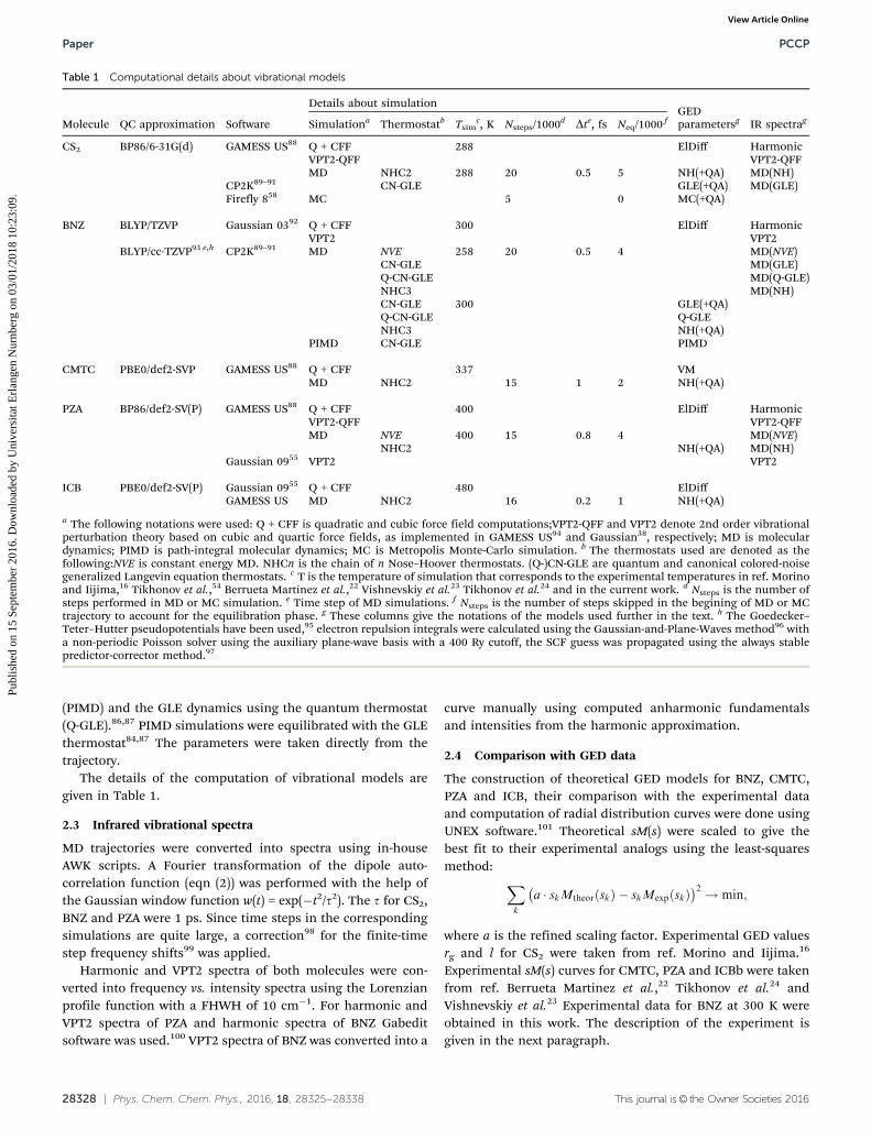
Table 1 Computational details about vibrational models

Molecule QC approximation Software

Details about simulationGEDparametersg IR spectragSimulationa Thermostatb Tsim

c, K Nsteps/1000d Dte, fs Neq/1000 f

CS2 BP86/6-31G(d) GAMESS US88 Q + CFF 288 ElDiff HarmonicVPT2-QFF VPT2-QFFMD NHC2 288 20 0.5 5 NH(+QA) MD(NH)

CP2K89–91 CN-GLE GLE(+QA) MD(GLE)Firefly 858 MC 5 0 MC(+QA)

BNZ BLYP/TZVP Gaussian 0392 Q + CFF 300 ElDiff HarmonicVPT2 VPT2

BLYP/cc-TZVP93 e,h CP2K89–91 MD NVE 258 20 0.5 4 MD(NVE)CN-GLE MD(GLE)Q-CN-GLE MD(Q-GLE)NHC3 MD(NH)CN-GLE 300 GLE(+QA)Q-CN-GLE Q-GLENHC3 NH(+QA)

PIMD CN-GLE PIMD

CMTC PBE0/def2-SVP GAMESS US88 Q + CFF 337 VMMD NHC2 15 1 2 NH(+QA)

PZA BP86/def2-SV(P) GAMESS US88 Q + CFF 400 ElDiff HarmonicVPT2-QFF VPT2-QFFMD NVE 400 15 0.8 4 MD(NVE)

NHC2 NH(+QA) MD(NH)Gaussian 0955 VPT2 VPT2

ICB PBE0/def2-SV(P) Gaussian 0955 Q + CFF 480 ElDiffGAMESS US MD NHC2 16 0.2 1 NH(+QA)

a The following notations were used: Q + CFF is quadratic and cubic force field computations;VPT2-QFF and VPT2 denote 2nd order vibrationalperturbation theory based on cubic and quartic force fields, as implemented in GAMESS US94 and Gaussian38, respectively; MD is moleculardynamics; PIMD is path-integral molecular dynamics; MC is Metropolis Monte-Carlo simulation. b The thermostats used are denoted as thefollowing:NVE is constant energy MD. NHCn is the chain of n Nose–Hoover thermostats. (Q-)CN-GLE are quantum and canonical colored-noisegeneralized Langevin equation thermostats. c T is the temperature of simulation that corresponds to the experimental temperatures in ref. Morinoand Iijima,16 Tikhonov et al.,54 Berrueta Martinez et al.,22 Vishnevskiy et al.23 Tikhonov et al.24 and in the current work. d Nsteps is the number ofsteps performed in MD or MC simulation. e Time step of MD simulations. f Nsteps is the number of steps skipped in the begining of MD or MCtrajectory to account for the equilibration phase. g These columns give the notations of the models used further in the text. h The Goedecker–Teter–Hutter pseudopotentials have been used,95 electron repulsion integrals were calculated using the Gaussian-and-Plane-Waves method96 witha non-periodic Poisson solver using the auxiliary plane-wave basis with a 400 Ry cutoff, the SCF guess was propagated using the always stablepredictor-corrector method.97

Paper PCCP

Publ

ishe

d on

15

Sept

embe

r 20

16. D

ownl

oade

d by

Uni

vers

itat E

rlan

gen

Nur

nber

g on

03/

01/2

018

10:2

3:09

. View Article Online

This journal is© the Owner Societies 2016 Phys. Chem. Chem. Phys., 2016, 18, 28325--28338 | 28329

2.4.1 GED experiment for BNZ. A sample of BNZ withpurity Z99.5% was purchased from Roth-Chemie GmbH andused with no further purification.

The electron diffraction patterns were recorded on the recentlyimproved Balzers Eldigraph KDG2 gas electron diffractometer.102,103

Data were collected at two different nozzle-to-detector distances,namely 250.0 (MD) and 500.0 mm (LD). The electron diffractionpatterns were measured on Fuji BAS IP MP 2025 imaging plates,which were scanned using a calibrated Fuji BAS 1800II scanner. Thetemperature of the experiment was maintained as close to 300 K aspossible in order to be applicable for multiple computations done inthe previous study.54

The intensity curves were obtained from scanned images byapplying the method described in detail elsewhere.104 Electronwavelengths were refined105 using diffraction patterns ofCCl4, recorded along with the substances under investigation.Background was extracted from total intensity curves using theUNEX program.101

The summary of experimental conditions is given in Table 2.

3 Results and discussion3.1 CS2: the simplest example

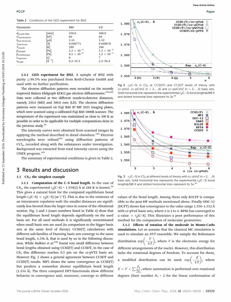
3.1.1 Computation of the C–S bond length. In the case ofCS2, the experimental rg(C–S) = 1.559(2) Å at 288 K is known.16

This gives a natural limit for the computed equilibrium bondlength re(C–S) o rg(C–S) (at 8 T). This is due to the existence ofan interatomic repulsion wall: the smaller distances are signifi-cantly less favored than the larger ones in course of the vibrationalmotion. Fig. 2 and 3 (exact numbers listed in Table 4) show thatthe equilibrium bond length depends significantly on the usedbasis set. For all used methods it is significantly overestimatedwhen small basis sets are used (in comparison to the bigger basissets at the same level of theory). CCSD(T) calculations withdifferent sub-families of Dunning basis sets converge to the samebond length, 1.556 Å, that is used by us in the following discus-sion. While Halkier et al.106 found very small difference betweenbond lengths obtained using CCSD(T) and CCSDT, in the case ofCS2 this difference reaches 0.5 pm on the cc-pVTZ basis set.However Fig. 2 shows a general agreement between CCSDT andCCSD(T) results. MP2 shows the same convergence as CCSD(T)but predicts a somewhat shorter equilibrium bond length(1.554 Å). The three compared DFT-functionals show differentbehavior in convergence and, moreover, converge to different

values of the bond length. Among them only B3LYP is compa-tible to the post-HF methods mentioned above. Finally ODC-12(DCFT) shows fast convergence to the value range 1.550–1.552 Åwith cc-pVnZ basis sets, where n is 2 to 4. BP86 has converged toa value 4 rg(C–S). This illustrates a poor performance of thismethod for the computation of molecular geometries.

3.1.2 Effects of rotation of the molecule in Monte-Carlosimulations. Let us assume that the classical MC simulation isused to simulate an NVT ensemble. We sample the Boltzmann

distribution exp � V

kT

� �, where V is the electronic energy for

different arrangements of the nuclei. However, this distributionlacks the rotational degrees of freedom. To account for them,

a modified distribution can be used: exp � E

kT

� �, where

E ¼ V þP Ja

2Ia, where summation is performed over rotational

degrees (their number Nr = 2 for the linear conformation of

Table 2 Conditions of the GED experiment for BNZ

Parameter MD LD

dnozzle-film [mm] 250.0 500.0Uacceleration [kV] 60 60Ifast electrons [mA] 1.53 1.52lelectrons [Å] 0.048771 0.048678Tnozzle [K] 299 298psample [Pa] 2.3 � 10�4 1.3 � 10�4

presidual gas [Pa] 8.1 � 10�6 1.2 � 10�5

texposure [s] 6 7srange [Å�1] 6.2–32.2 2.2–16.4

Fig. 2 re(C–S) in CS2 at CCSD(T) and CCSDT levels of theory withcc-pVnZ, cc-pCVnZ (n = 2,. . .,6) and cc-pwCVnZ (n = 2,. . .,5) basis sets.Solid horizontal line represents the experimental rg(C–S) bond length@288 Kand dotted horizontal lines represent its 3s.16

Fig. 3 re(C–S) in CS2 at different levels of theory with cc-pVnZ (n = 2,. . .,6)basis sets. Solid horizontal line represents the experimental rg(C–S) bondlength@288 K and dotted horizontal lines represent its 3s.16

PCCP Paper

Publ

ishe

d on

15

Sept

embe

r 20

16. D

ownl

oade

d by

Uni

vers

itat E

rlan

gen

Nur

nber

g on

03/

01/2

018

10:2

3:09

. View Article Online

28330 | Phys. Chem. Chem. Phys., 2016, 18, 28325--28338 This journal is© the Owner Societies 2016

atoms and Nr = 3 in the other cases), Ia is the main moment ofinertia for the molecule. Averaging over the rotational degreesof freedom at certain arrangement of the nuclei leads to

the probability distribution /ffiffiffiffiffiffiffiffiffiffiffiPaIap

exp � V

kT

� �.108 Here, the

rotation is treated with classical mechanics. In the case ofMetropolis Monte-Carlo sampling, each configuration shouldbe weighted using the function f ¼

ffiffiffiffiffiffiffiffiffiffiffiPaIap

. Therefore each

observable is computed as hXi ¼ hX � f ih f i , where X is the

observed value and h. . .i denotes averaging over the MC trajec-tory. In the case of CS2, the rg–re correction for the C–S bondfor the MC model without the weighting of the frames with f is0.12 pm, while the value obtained with weighting is 0.17 pm.

The difference of ca. 0.05 pm is of the same order of magnitudeas the correction for the rotation of the molecule obtainedusing VibModule software (0.03 pm). Thus, we find this treat-ment of rotation in the MC simulations suitable for the roughestimation of the rotational effects.

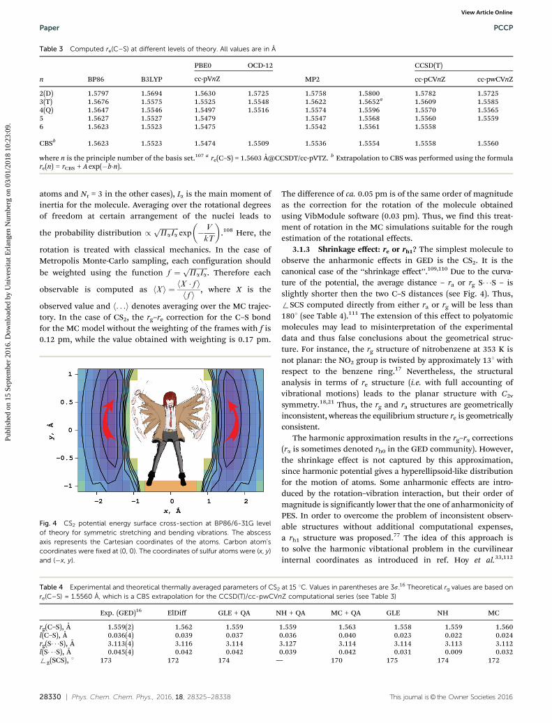
3.1.3 Shrinkage effect: re or rh1? The simplest molecule toobserve the anharmonic effects in GED is the CS2. It is thecanonical case of the ‘‘shrinkage effect’’.109,110 Due to the curva-ture of the potential, the average distance – ra or rg S� � �S – isslightly shorter then the two C–S distances (see Fig. 4). Thus,+SCS computed directly from either ra or rg will be less than1801 (see Table 4).111 The extension of this effect to polyatomicmolecules may lead to misinterpretation of the experimentaldata and thus false conclusions about the geometrical struc-ture. For instance, the rg structure of nitrobenzene at 353 K isnot planar: the NO2 group is twisted by approximately 131 withrespect to the benzene ring.17 Nevertheless, the structuralanalysis in terms of re structure (i.e. with full accounting ofvibrational motions) leads to the planar structure with C2v

symmetry.18,21 Thus, the rg and ra structures are geometricallyinconsistent, whereas the equilibrium structure re is geometricallyconsistent.

The harmonic approximation results in the rg–ra corrections(ra is sometimes denoted rh0 in the GED community). However,the shrinkage effect is not captured by this approximation,since harmonic potential gives a hyperellipsoid-like distributionfor the motion of atoms. Some anharmonic effects are intro-duced by the rotation–vibration interaction, but their order ofmagnitude is significantly lower that the one of anharmonicity ofPES. In order to overcome the problem of inconsistent observ-able structures without additional computational expenses,a rh1 structure was proposed.77 The idea of this approach isto solve the harmonic vibtational problem in the curvilinearinternal coordinates as introduced in ref. Hoy et al.33,112

Table 3 Computed re(C–S) at different levels of theory. All values are in Å

n BP86 B3LYP

PBE0 OCD-12

MP2

CCSD(T)

cc-pVnZ cc-pCVnZ cc-pwCVnZ

2(D) 1.5797 1.5694 1.5630 1.5725 1.5758 1.5800 1.5782 1.57253(T) 1.5676 1.5575 1.5525 1.5548 1.5622 1.5652a 1.5609 1.55854(Q) 1.5647 1.5546 1.5497 1.5516 1.5574 1.5596 1.5570 1.55655 1.5627 1.5527 1.5479 1.5547 1.5568 1.5560 1.55596 1.5623 1.5523 1.5475 1.5542 1.5561 1.5558

CBSb 1.5623 1.5523 1.5474 1.5509 1.5536 1.5554 1.5558 1.5560

where n is the principle number of the basis set.107 a re(C–S) = 1.5603 Å@CCSDT/cc-pVTZ. b Extrapolation to CBS was performed using the formulare(n) = rCBS + A exp(�b�n).

Fig. 4 CS2 potential energy surface cross-section at BP86/6-31G levelof theory for symmetric stretching and bending vibrations. The abscessaxis represents the Cartesian coordinates of the atoms. Carbon atom’scoordinates were fixed at (0, 0). The coordinates of sulfur atoms were (x, y)and (�x, y).

Table 4 Experimental and theoretical thermally averaged parameters of CS2 at 15 1C. Values in parentheses are 3s.16 Theoretical rg values are based onre(C–S) = 1.5560 Å, which is a CBS extrapolation for the CCSD(T)/cc-pwCVnZ computational series (see Table 3)

Exp. (GED)16 ElDiff GLE + QA NH + QA MC + QA GLE NH MC

rg(C–S), Å 1.559(2) 1.562 1.559 1.559 1.563 1.558 1.559 1.560l(C–S), Å 0.036(4) 0.039 0.037 0.036 0.040 0.023 0.022 0.024rg(S� � �S), Å 3.113(4) 3.116 3.114 3.127 3.114 3.114 3.113 3.112l(S� � �S), Å 0.045(4) 0.042 0.042 0.039 0.042 0.031 0.009 0.032+g(SCS), 1 173 172 174 — 170 175 174 172

Paper PCCP

Publ

ishe

d on

15

Sept

embe

r 20

16. D

ownl

oade

d by

Uni

vers

itat E

rlan

gen

Nur

nber

g on

03/

01/2

018

10:2

3:09

. View Article Online

This journal is© the Owner Societies 2016 Phys. Chem. Chem. Phys., 2016, 18, 28325--28338 | 28331

These coordinates are related to the Cartesian coordinates as

qi ¼Pk

@qi

@akDak þ

1

2

Pk

Pl

@2qi

@ak@alDakDal , where qi is the internal

curvilinear coordinate, ak is one of the Cartesian coordinates,and Dak is the deviation from the reference value. Vibrationalproblem is modified by the effective anharmonic term, theso-called ‘‘kinematic anharmonicity’’. It consists of sum ofelements ppiq j pk, where pi is the corresponding momentum ofcoordinate qi. This anharmonic term arises, when the problem istreated in the internal coordinates. After that, perturbation theoryis applied to obtain the shrinkage corrections.80

The standard implementation of the described algorithm isShrink software written in Fortran.77–80 In this work we use arecent C implementation in the VibModule program76 as well asElDiff software.15 The CS2 molecule was chosen to demonstrate therelation between different methods for calculation of the correc-tions. The results are presented in Table 5. VibModule uses onlythe curvilinear internal coordinates. Therefore only two types ofcorrections were computed with this software. Others were com-puted with ElDiff.� rg�ra (using only the quadratic field).� rg�rh1 (using only the quadratic field).� rg�re (using the quadratic and cubic force fields), which is

equvalent to the VM model.Obviously, the use of Cartesian coordinates and linearized

internal coordinates must result in almost similar results, sincethe coordinates are connected by a unitary transformation.Nevertheless, they still have been used in a separate fashionyielding the same values for the corrections. The computationsusing only the harmonic force field in Cartesian and linearizedinternal coordinates gave rg�ra corrections, whereas the curvi-linear coordinates gave rg�rh1 values. The computation of rg�re

corrections in all 3 types of coordinates using the quadratic andcubic force fields obviously resulted in the same values, whichwere in turn equal to the result of the VibModule computation.As we can see, rg�re, rg�rh1 and rg�ra are very different fromeach other. But if we compute rg�re corrections (or equivalentlyra�re) using other quantum methods, such as PIMD, we willobtain very similar values at the same QC approximation (seeref. Tikhonov et al.54 or ESI† for an example). It is due to theclear physical definition of rg, ra and re values that allows them to becomputed. The rh1 structure is coordinate-dependent and cannotbe computed directly. The ra structure is coordinate independent,

but is geometrically inconsistent. Also, the re structure correspondsto the optimized structure obtained from QC calculations, whetherrh1 and ra cannot be compared with the calculations directly.

Of course, computation of the harmonic force field is signifi-cantly cheaper than the cubic one, let alone MD an MC simula-tions. Still, we assume that it is more convenient to compute thecubic force field or perform MD or MC simulations at a lower QCapproximation in order to obtain ra�re corrections in order toperform a direct comparison of the experimental and computedvalues obtained.

3.1.4 Comparison with the experiment. The results for CS2

are presented in Table 4. The theoretical rg distances, ampli-tudes l and shrinkage angles +g(SCS) computed from rg valueswere compared with the corresponding experimental values.16

All the shrinkage angles (both quantum and classical, except forNH + QA) were found to be in good agreement with the experi-mental one and with each other. The GLE + QA and MC + QAvalues were slightly smaller then the corresponding classicalvalues as it was expected. It is important to note that the qualityof the thermostat plays a very important role for the resultingvalues of rg and ra structures. As we can see the amplitude of S� � �Svibrations in the case of NH was significantly smaller than thoseobserved for GLE and MC. This is can be either a result of the‘‘flying ice cube’’ effect113 (a bad energy redistribution betweenthe degrees of freedom by the thermostat) or the nonergodictrajectory for such few number of degrees of freedom114 ortheir combination. Therefore the extrapolation of quantumeffects performed by Qassandra for the NH model becomesunstable. This leads to unphysical rg�re corrections that makerg(S� � �S) 4 2rg(C–S).

All the theoretical quantum mean vibrational amplitudes werein significantly better correlation with each other and with experi-mental data, than those observed for GLE, MC and especially NH.NH + QA for the l-s has performed unexpectedly better than therg�re corrections at the same level of theory.

3.2 Four benchmark molecules

The direct comparison of the terms in the molecules with morethen 3 atoms becomes quite boring and inefficient. Thereforesimilar to the previous work we have performed the comparisonof different pure theoretical models for sM(s) with experimentaldata. The similarity of the theoretical model with experimentaldata was measured using a structural R-factor:

Rf ¼

ffiffiffiffiffiffiffiffiffiffiffiffiffiffiffiffiffiffiffiffiffiffiffiffiffiffiffiffiffiffiffiffiffiffiffiffiffiffiffiffiffiffiffiffiffiffiffiffiffiffiffiffiffiffiffiffiffiffiffiffiffiffiffiffiffiffiffiffiffiffiffiPMk¼1

skMexp skð Þ � a � skMtheor skð Þ� �2

PMk¼1

skMexp2 skð Þ

vuuuuuut � 100%; (8)

where a is the refined scaling factor. The basic theoreticalmodel in GED is ‘‘re geometry’’ + ‘‘vibrational parameters(l, ra�re, k)’’. Different optimized structures were obtainedusing two post-Hartree–Fock methods (in our case – CCSD(T)and MP2) and several popular DFT functionals (B3LYP, PBE0and BP86) and a very popular cc-pVTZ (and SDB-cc-pVTZ forICB) basis set. They were used to construct different theoretical

Table 5 Theoretical rg�re, rg�rh1 and rg�ra corrections for CS2 at 15 1C.All values are in pm

Term

Harmonic

Anharmonica rg�re

Linearb rg�ra Curvilinear rg�rh1

ElDiff ElDiff VibModule

C–S 0.36 0.07 0.04 0.56S� � �S 0.00 �0.59 �0.65 0.39

a The corresponding values were found to be the same for ElDiff withusage of Cartesian, linear and curvilineal internal coordinates as well asfor VibModule. b The same values were obtained for Cartesian coordi-nates using ElDiff.

PCCP Paper

Publ

ishe

d on

15

Sept

embe

r 20

16. D

ownl

oade

d by

Uni

vers

itat E

rlan

gen

Nur

nber

g on

03/

01/2

018

10:2

3:09

. View Article Online

28332 | Phys. Chem. Chem. Phys., 2016, 18, 28325--28338 This journal is© the Owner Societies 2016

models in order to be sure that the observed tendencies in theRf are not random. The QC approximations for computation ofl, ra�re, and k were sufficiently less computationally expensive.This is a very common practice in GED that gives quite goodresults.22–24,54

A visualization of the results of GED analysis was done usingthe so-called radial distribution function f (r):12

f ðrÞ ¼ð10

sMðsÞ sinðsrÞ expð�b � s2Þds;

which is a sine-Fourier transformation of sM(s) with a Gaussianwindow function exp(�b�s2) and b controls the width of thewindow. The physical meaning of f (r) is the sum of P(r)/rweighted for the scattering ability of the pairs of atoms (seeIntroduction). The results obtained for Rf-s can be found inTable 6 and the f (r)-s for the best available ab initio re structureare given in Fig. 5–8.

Table 6 Structural Rf (eqn (8)) for BNZ, CMTC, PZA and ICB with differenttheoretical geometries and vibrational parameters. cc-pVTZ (and SBD-cc-pVTZ for the ICB) basis set was used. All values are in %

Molecule Vibrational parameters CCSD(T) MP2 PBE0 B3LYP BP86

BNZ ElDiff 6.8 7.2 9.6 6.8 13.2PIMD 8.1 7.0 13.5 9.2 9.3Q-GLE 10.0 8.9 14.6 10.8 10.4GLE + QA 9.1 10.0 8.1 7.9 16.7NH + QA 10.3 9.1 15.0 11.1 9.8GLE 19.5 19.8 19.7 19.1 23.5NH 22.4 21.5 26.4 23.3 20.5

CMTC VM 14.2 14.4 13.7 29.0 34.0NH + QA 9.8 13.1 14.9 23.2 27.0NH 15.5 17.4 13.8 28.3 33.0

PZA ElDiff 8.9 8.2 6.5 16.1NH + QA 7.4 9.2 5.7 14.0NH 16.2 16.5 14.9 19.7

ICB ElDiff 9.2 12.2 19.4 21.3NH + QA 12.8 16.4 19.8 19.3NH 19.8 23.5 24.5 23.6

Fig. 5 Experimental (triangles) and theoretical (lines) radial distribution curvesand their differences (experimental vs. theoretical) for BNZ. Theoretical modelswere based on CCSD(T)/cc-pVTZ equilibrium geometry.

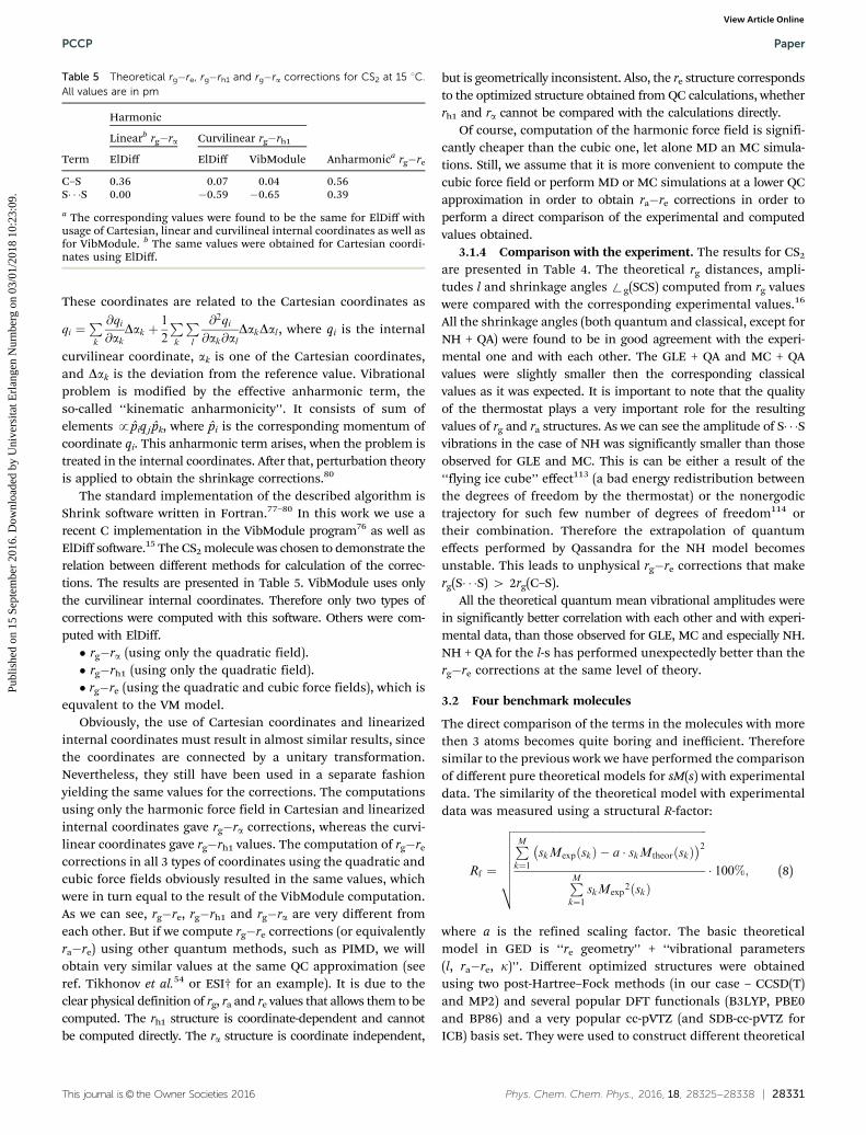
Fig. 6 Experimental (triangles) and theoretical (lines) radial distribution curvesand their differences (experimental vs. theoretical) for CMTC. Theoreticalmodels were based on CCSD(T)/cc-pVTZ equilibrium geometry.

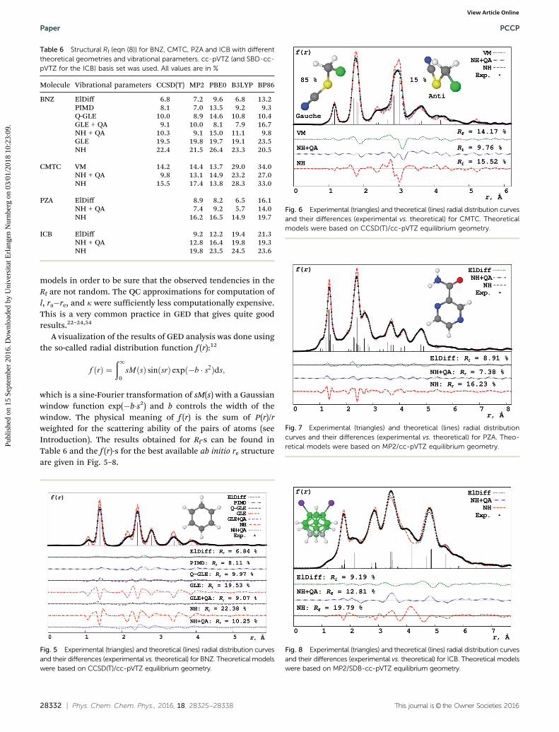
Fig. 7 Experimental (triangles) and theoretical (lines) radial distributioncurves and their differences (experimental vs. theoretical) for PZA. Theo-retical models were based on MP2/cc-pVTZ equilibrium geometry.

Fig. 8 Experimental (triangles) and theoretical (lines) radial distribution curvesand their differences (experimental vs. theoretical) for ICB. Theoretical modelswere based on MP2/SDB-cc-pVTZ equilibrium geometry.

Paper PCCP

Publ

ishe

d on

15

Sept

embe

r 20

16. D

ownl

oade

d by

Uni

vers

itat E

rlan

gen

Nur

nber

g on

03/

01/2

018

10:2

3:09

. View Article Online

This journal is© the Owner Societies 2016 Phys. Chem. Chem. Phys., 2016, 18, 28325--28338 | 28333

3.2.1 Rigid molecules. For the rigid molecules (i.e. BNZ, PZAand ICB) we can see that the tendency is that all the models thataccount for quantum vibrational effects (ElDiff, PIMD, Q-GLE,NH + QA and GLE + QA) give sufficiently better consistency withthe experiment than the classical ones (NH and GLE). Theinfluence of quantum effects can be easily seen from f (r): thepeaks from classical models are sufficiently more narrow thanfrom the quantum ones. The ElDiff still gives the best agree-ment with the experiment in cases of the rigid systems. This isprobably the result of the stochastic nature of MD simula-tions: they give the best result only for the infinite length of thetrajectory. Besides, they depend on the performance of thethermostats used. But still the agreement of the MD-basedmodels is satisfactory: they capture most of the vibrationalmotions’ behavior.

We can also see some tendencies for the quality of the pre-dicted geometries from the analysis of Table 6. First of all,MP2 and B3LYP on the chosen set of molecules performsufficiently well for the molecules that consist of the atomsfrom the 1st and 2nd rows of the periodic table. But, B3LYPfails in the case of ICB. PBE0, on the other hand, gives quitereasonable geometries for BNZ, PZA and ICB. BP86 is found togive bad geometries. These observations are in good correlationwith those for CS2.

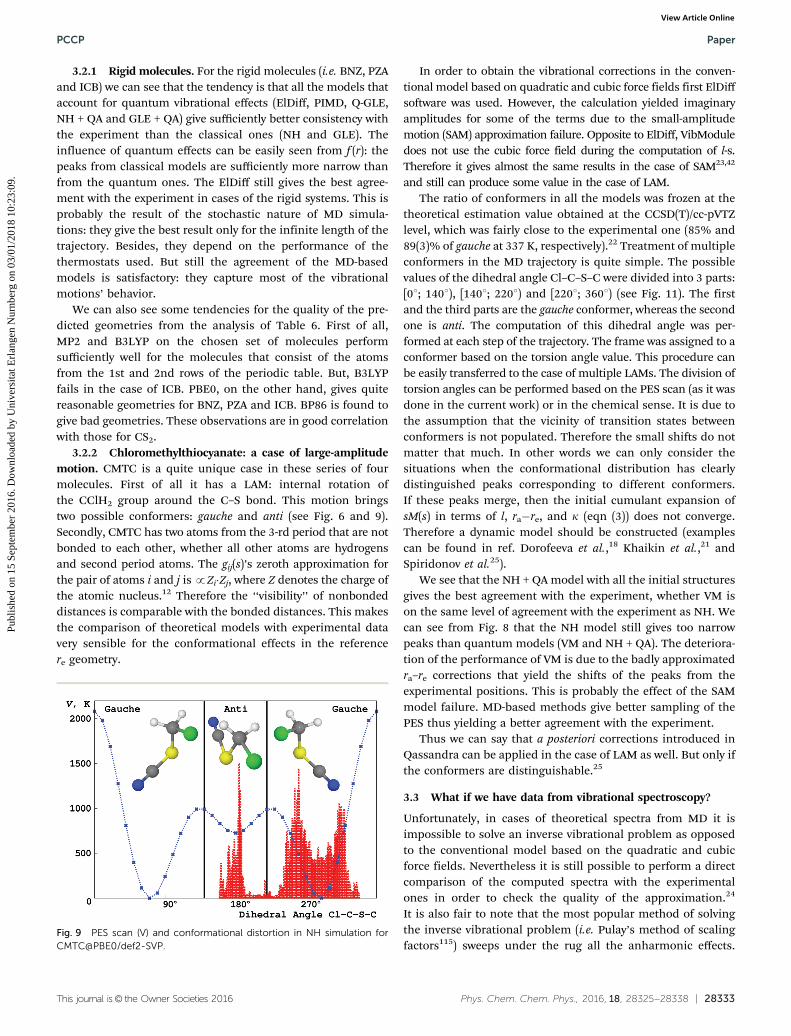
3.2.2 Chloromethylthiocyanate: a case of large-amplitudemotion. CMTC is a quite unique case in these series of fourmolecules. First of all it has a LAM: internal rotation ofthe CClH2 group around the C–S bond. This motion bringstwo possible conformers: gauche and anti (see Fig. 6 and 9).Secondly, CMTC has two atoms from the 3-rd period that are notbonded to each other, whether all other atoms are hydrogensand second period atoms. The gij(s)’s zeroth approximation forthe pair of atoms i and j is pZi�Zj, where Z denotes the charge ofthe atomic nucleus.12 Therefore the ‘‘visibility’’ of nonbondeddistances is comparable with the bonded distances. This makesthe comparison of theoretical models with experimental datavery sensible for the conformational effects in the referencere geometry.

In order to obtain the vibrational corrections in the conven-tional model based on quadratic and cubic force fields first ElDiffsoftware was used. However, the calculation yielded imaginaryamplitudes for some of the terms due to the small-amplitudemotion (SAM) approximation failure. Opposite to ElDiff, VibModuledoes not use the cubic force field during the computation of l-s.Therefore it gives almost the same results in the case of SAM23,42

and still can produce some value in the case of LAM.The ratio of conformers in all the models was frozen at the

theoretical estimation value obtained at the CCSD(T)/cc-pVTZlevel, which was fairly close to the experimental one (85% and89(3)% of gauche at 337 K, respectively).22 Treatment of multipleconformers in the MD trajectory is quite simple. The possiblevalues of the dihedral angle Cl–C–S–C were divided into 3 parts:[01; 1401), [1401; 2201) and [2201; 3601) (see Fig. 11). The firstand the third parts are the gauche conformer, whereas the secondone is anti. The computation of this dihedral angle was per-formed at each step of the trajectory. The frame was assigned to aconformer based on the torsion angle value. This procedure canbe easily transferred to the case of multiple LAMs. The division oftorsion angles can be performed based on the PES scan (as it wasdone in the current work) or in the chemical sense. It is due tothe assumption that the vicinity of transition states betweenconformers is not populated. Therefore the small shifts do notmatter that much. In other words we can only consider thesituations when the conformational distribution has clearlydistinguished peaks corresponding to different conformers.If these peaks merge, then the initial cumulant expansion ofsM(s) in terms of l, ra�re, and k (eqn (3)) does not converge.Therefore a dynamic model should be constructed (examplescan be found in ref. Dorofeeva et al.,18 Khaikin et al.,21 andSpiridonov et al.25).

We see that the NH + QA model with all the initial structuresgives the best agreement with the experiment, whether VM ison the same level of agreement with the experiment as NH. Wecan see from Fig. 8 that the NH model still gives too narrowpeaks than quantum models (VM and NH + QA). The deteriora-tion of the performance of VM is due to the badly approximatedra–re corrections that yield the shifts of the peaks from theexperimental positions. This is probably the effect of the SAMmodel failure. MD-based methods give better sampling of thePES thus yielding a better agreement with the experiment.

Thus we can say that a posteriori corrections introduced inQassandra can be applied in the case of LAM as well. But only ifthe conformers are distinguishable.25

3.3 What if we have data from vibrational spectroscopy?

Unfortunately, in cases of theoretical spectra from MD it isimpossible to solve an inverse vibrational problem as opposedto the conventional model based on the quadratic and cubicforce fields. Nevertheless it is still possible to perform a directcomparison of the computed spectra with the experimentalones in order to check the quality of the approximation.24

It is also fair to note that the most popular method of solvingthe inverse vibrational problem (i.e. Pulay’s method of scalingfactors115) sweeps under the rug all the anharmonic effects.

Fig. 9 PES scan (V) and conformational distortion in NH simulation forCMTC@PBE0/def2-SVP.

PCCP Paper

Publ

ishe

d on

15

Sept

embe

r 20

16. D

ownl

oade

d by

Uni

vers

itat E

rlan

gen

Nur

nber

g on

03/

01/2

018

10:2

3:09

. View Article Online

28334 | Phys. Chem. Chem. Phys., 2016, 18, 28325--28338 This journal is© the Owner Societies 2016

It is due to the fact that usually only the harmonic frequenciesare fitted to the experimental ones.18,20,21 But the anharmoniceffect can be very important for the successful assignment ofthe peaks.36,37

The two basic recommendations for the computation of VSpfrom MD are:99,116

� use small time steps.� obtain several of constant energy MD (i.e. NVE) trajectories

under different initial conditions, compute spectra from eachof the trajectories and then average them;

The first recommendation reflects the fact that the large timesteps shift the vibrational peaks in spectra towards a higherfrequency range.49,99 This behavior, however can be corrected

using a correction ncorr ¼ffiffiffiffiffiffiffiffiffiffiffiffiffiffiffiffiffiffiffiffiffiffiffiffiffiffiffiffiffiffiffiffiffiffiffiffiffiffiffiffiffiffiffiffiffiffiffiffiffiffiffiffi2 � 1� cos 2p � Dt � ninið Þð Þ

p2p � Dt , where

n are the initial (ini) and corrected (corr) frequencies and Dt isthe time step used in the MD simulation.98 The only restrictionin this case is Dt o 1/(pnmax) = tmin/p, where nmax and tmin are thefrequency and the period of the fastest motion in the system,respectively.98

In cases with GED experimental data presented it is moreconvenient to perform only one NVT simulation instead. It isdue to the fact that NVE trajectories cannot be used for thecomputation of l, re�ra, and k. The usage of thermostated NVTMD for the computation of VSp is not novel itself.52,117 The aimwas to check the performance of the thermostats that give goodresults for GED as found in this and the previous study54

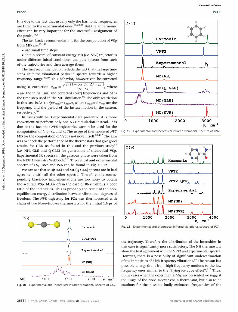
(i.e. NH, GLE and Q-GLE) for generation of theoretical VSp.Experimental IR spectra in the gaseous phase were taken fromthe NIST Chemistry Webbook.118 Theoretical and experimentalspectra of CS2, BNZ and PZA can be found in Fig. 10–12.

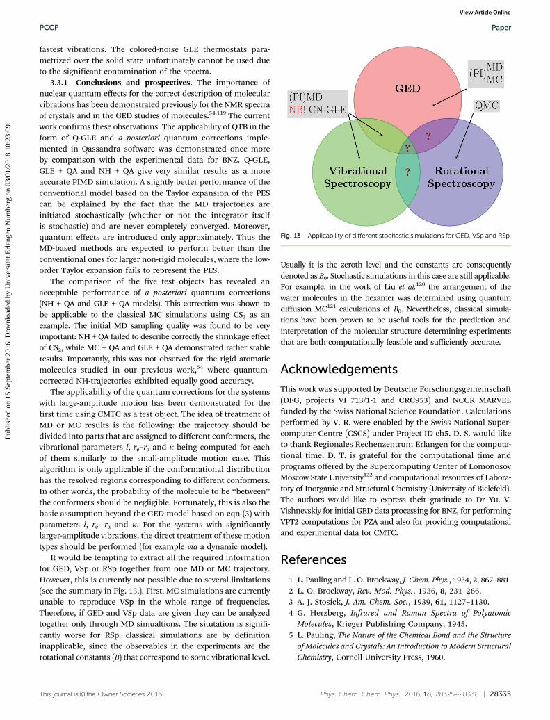
We can see that MD(GLE) and MD(Q-GLE) spectra are in badagreement with all the other spectra. Therefore, the corres-ponding black-box implementations are too noisy to obtainthe accurate VSp. MD(NVE) in the case of BNZ exhibits a poorratio of the intensities. This is probably the result of the non-equilibrium energy distribution between vibrational degrees offreedom. The NVE trajectory for PZA was thermostatted withchain of two Nose–Hoover thermostats for the initial 1.6 ps of

the trajectory. Therefore the distribution of the intensities inthis case is significantly more satisfactory. The NH thermostatsshow the best agreement with the VPT2 and experimental spectra.However, there is a possibility of significant underestimationof the intensities of high-frequency vibrations.98 The reason is apossible energy drain from high-frequency motions to the lowfrequency ones similar to the ‘‘flying ice cube effect’’.113 Thus,in the cases when the experimental VSp are presented we suggestthe usage of the Nose–Hoover chain thermostat, but also to becautious for the possible badly estimated frequencies of theFig. 10 Experimental and theoretical infrared vibrational spectra of CS2.

Fig. 11 Experimental and theoretical infrared vibrational spectra of BNZ.

Fig. 12 Experimental and theoretical infrared vibrational spectra of PZA.

Paper PCCP

Publ

ishe

d on

15

Sept

embe

r 20

16. D

ownl

oade

d by

Uni

vers

itat E

rlan

gen

Nur

nber

g on

03/

01/2

018

10:2

3:09

. View Article Online

This journal is© the Owner Societies 2016 Phys. Chem. Chem. Phys., 2016, 18, 28325--28338 | 28335

fastest vibrations. The colored-noise GLE thermostats para-metrized over the solid state unfortunately cannot be used dueto the significant contamination of the spectra.

3.3.1 Conclusions and prospectives. The importance ofnuclear quantum effects for the correct description of molecularvibrations has been demonstrated previously for the NMR spectraof crystals and in the GED studies of molecules.54,119 The currentwork confirms these observations. The applicability of QTB in theform of Q-GLE and a posteriori quantum corrections imple-mented in Qassandra software was demonstrated once moreby comparison with the experimental data for BNZ. Q-GLE,GLE + QA and NH + QA give very similar results as a moreaccurate PIMD simulation. A slightly better performance of theconventional model based on the Taylor expansion of the PEScan be explained by the fact that the MD trajectories areinitiated stochastically (whether or not the integrator itselfis stochastic) and are never completely converged. Moreover,quantum effects are introduced only approximately. Thus theMD-based methods are expected to perform better than theconventional ones for larger non-rigid molecules, where the low-order Taylor expansion fails to represent the PES.

The comparison of the five test objects has revealed anacceptable performance of a posteriori quantum corrections(NH + QA and GLE + QA models). This correction was shown tobe applicable to the classical MC simulations using CS2 as anexample. The initial MD sampling quality was found to be veryimportant: NH + QA failed to describe correctly the shrinkage effectof CS2, while MC + QA and GLE + QA demonstrated rather stableresults. Importantly, this was not observed for the rigid aromaticmolecules studied in our previous work,54 where quantum-corrected NH-trajectories exhibited equally good accuracy.

The applicability of the quantum corrections for the systemswith large-amplitude motion has been demonstrated for thefirst time using CMTC as a test object. The idea of treatment ofMD or MC results is the following: the trajectory should bedivided into parts that are assigned to different conformers, thevibrational parameters l, re–ra and k being computed for eachof them similarly to the small-amplitude motion case. Thisalgorithm is only applicable if the conformational distributionhas the resolved regions corresponding to different conformers.In other words, the probability of the molecule to be ‘‘between’’the conformers should be negligible. Fortunately, this is also thebasic assumption beyond the GED model based on eqn (3) withparameters l, re�ra and k. For the systems with significantlylarger-amplitude vibrations, the direct treatment of these motiontypes should be performed (for example via a dynamic model).

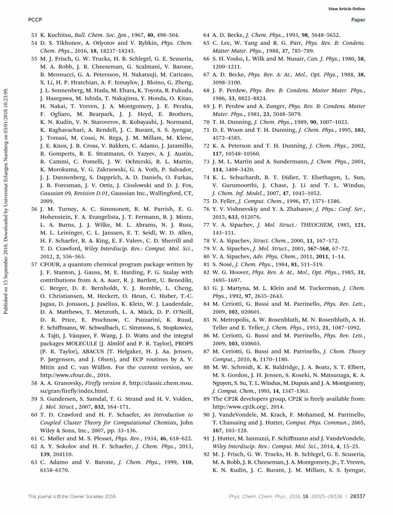
It would be tempting to extract all the required informationfor GED, VSp or RSp together from one MD or MC trajectory.However, this is currently not possible due to several limitations(see the summary in Fig. 13.). First, MC simulations are currentlyunable to reproduce VSp in the whole range of frequencies.Therefore, if GED and VSp data are given they can be analyzedtogether only through MD simualtions. The situtation is signifi-cantly worse for RSp: classical simulations are by definitioninapplicable, since the observables in the experiments are therotational constants (B) that correspond to some vibrational level.

Usually it is the zeroth level and the constants are consequentlydenoted as B0. Stochastic simulations in this case are still applicable.For example, in the work of Liu et al.120 the arrangement of thewater molecules in the hexamer was determined using quantumdiffusion MC121 calculations of B0. Nevertheless, classical simula-tions have been proven to be useful tools for the prediction andinterpretation of the molecular structure determining experimentsthat are both computationally feasible and sufficiently accurate.

Acknowledgements

This work was supported by Deutsche Forschungsgemeinschaft(DFG, projects VI 713/1-1 and CRC953) and NCCR MARVELfunded by the Swiss National Science Foundation. Calculationsperformed by V. R. were enabled by the Swiss National Super-computer Centre (CSCS) under Project ID ch5. D. S. would liketo thank Regionales Rechenzentrum Erlangen for the computa-tional time. D. T. is grateful for the computational time andprograms offered by the Supercomputing Center of LomonosovMoscow State University122 and computational resources of Labora-tory of Inorganic and Structural Chemistry (University of Bielefeld).The authors would like to express their gratitude to Dr Yu. V.Vishnevskiy for initial GED data processing for BNZ, for performingVPT2 computations for PZA and also for providing computationaland experimental data for CMTC.

References

1 L. Pauling and L. O. Brockway, J. Chem. Phys., 1934, 2, 867–881.2 L. O. Brockway, Rev. Mod. Phys., 1936, 8, 231–266.3 A. J. Stosick, J. Am. Chem. Soc., 1939, 61, 1127–1130.4 G. Herzberg, Infrared and Raman Spectra of Polyatomic

Molecules, Krieger Publishing Company, 1945.5 L. Pauling, The Nature of the Chemical Bond and the Structure

of Molecules and Crystals: An Introduction to Modern StructuralChemistry, Cornell University Press, 1960.

Fig. 13 Applicability of different stochastic simulations for GED, VSp and RSp.

PCCP Paper

Publ

ishe

d on

15

Sept

embe

r 20

16. D

ownl

oade

d by

Uni

vers

itat E

rlan

gen

Nur

nber

g on

03/

01/2

018

10:2

3:09

. View Article Online

28336 | Phys. Chem. Chem. Phys., 2016, 18, 28325--28338 This journal is© the Owner Societies 2016

6 R. J. Gillespie and I. Hargittai, The VSEPR Model of Mole-cular Geometry, Dover Publications, Incorporated, 2012.

7 I. Hargittai, in Gas-Phase Electron Diffraction for MolecularStructure Determination, ed. T. E. Weirich, J. L. Labar andX. Zou, Springer, Netherlands, Dordrecht, 2006, pp. 197–206.

8 M. J. S. Dewar and W. Thiel, J. Am. Chem. Soc., 1977, 99,4899–4907.

9 M. J. S. Dewar and W. Thiel, J. Am. Chem. Soc., 1977, 99,4907–4917.

10 M. J. S. Dewar, E. G. Zoebisch, E. F. Healy and J. J. P. Stewart,J. Am. Chem. Soc., 1985, 107, 3902–3909.

11 H. S. Yu, X. He and D. G. Truhlar, J. Chem. Theory Comput.,2016, 12, 1280–1293.

12 I. Hargittai, in Stereochemical Applications of Gas PhaseElectron Diffraction, Part A: The Electron Diffraction Techni-que, ed. I. Hargittai and M. Hargittai, VCH Publishers, Inc.,New York, 1988.

13 R. S. Drago, Physical methods for chemists, Saunders CollegePub., 1992.

14 A. G. Yagola, I. V. Kochikov, G. M. Kuramshina andY. A. Pentin, Inverse problems of vibrational spectroscopy,VSP BV, 1999.

15 I. V. Kochikov, Y. I. Tarasov, G. M. Kuramshina, V. P.Spiridonov, A. G. Yagola and T. G. Strand, J. Mol. Struct.,1998, 445, 243–258.

16 Y. Morino and T. Iijima, Bull. Chem. Soc. Jpn., 1962, 35,1661–1667.

17 A. Domenicano, G. Schultz, I. Hargittai, M. Colapietro,G. Portalone, P. George and C. W. Bock, Struct. Chem.,1990, 1, 107–122.

18 O. V. Dorofeeva, Y. Vishnevskiy, N. Vogt, J. Vogt, L. Khristenko,S. Krasnoshchekov, I. Shishkov, I. Hargittai and L. Vilkov,Struct. Chem., 2007, 18, 739–753.

19 Y. I. Tarasov, I. V. Kochikov, D. M. Kovtun, N. Vogt,B. K. Novosadov and A. S. Saakyan, J. Struct. Chem., 2004,45, 778–785.

20 N. Vogt, L. S. Khaikin, O. E. Grikina and A. N. Rykov, J. Mol.Struct., 2013, 1050, 114–121.

21 L. S. Khaikin, I. V. Kochikov, O. E. Grikina, D. S. Tikhonovand E. G. Baskir, Struct. Chem., 2015, 26, 1651–1687.

22 Y. Berrueta Martinez, L. S. Rodriguez Pirani, M. F. Erben,C. G. Reuter, Y. V. Vishnevskiy, H. G. Stammler, N. W. Mitzeland C. O. Della Vedova, Phys. Chem. Chem. Phys., 2015, 17,15805–15812.

23 Y. V. Vishnevskiy, D. S. Tikhonov, C. G. Reuter, N. W. Mitzel,D. Hnyk, J. Holub, D. A. Wann, P. D. Lane, R. J. F. Berger andS. A. Hayes, Inorg. Chem., 2015, 54, 11868–11874.

24 D. S. Tikhonov, Y. V. Vishnevskiy, A. N. Rykov, O. E. Grikinaand L. S. Khaikin, J. Mol. Struct., 2016, DOI: 10.1016/j.molstruc.2016.05.090.

25 V. P. Spiridonov, A. A. Ishchenko and E. Z. Zasorin, Russ.Chem. Rev., 1978, 47, 54.

26 N. Vogt, J. Mol. Struct., 2001, 570, 189–195.27 F. Pawłowski, P. Jørgensen, J. Olsen, F. Hegelund, T. Helgaker,

J. Gauss, K. L. Bak and J. F. Stanton, J. Chem. Phys., 2002, 116,6482–6496.

28 D. G. Artiukhin, J. Kłos, E. J. Bieske and A. A. Buchachenko,J. Phys. Chem. A, 2014, 118, 6711–6720.

29 L. A. Surin, A. Potapov, A. A. Dolgov, I. V. Tarabukin, V. A.Panfilov, S. Schlemmer, Y. N. Kalugina, A. Faure andA. van der Avoird, J. Chem. Phys., 2015, 142, 114308.

30 L. A. Surin, I. V. Tarabukin, V. A. Panfilov, S. Schlemmer,Y. N. Kalugina, A. Faure, C. Rist and A. van der Avoird,J. Chem. Phys., 2015, 143, 154303.

31 J. C. D. E. Bright Wilson, Jr., Molecular Vibrations: The Theoryof Infrared and Raman Vibrational Spectra, Dover Publications,1980.

32 P. Atkins and J. De Paula, Physical Chemistry, OxfordUniversity Press, 8th edn, 2006.

33 P. R. Bunker and P. Jensen, Molecular Symmetry and Spectros-copy, NRC Research Press, 2nd edn, 2016, p. 748.

34 I. V. Kochikov, Y. I. Tarasov, N. Vogt and V. P. Spiridonov,J. Mol. Struct., 2002, 607, 163–174.

35 C. Puzzarini and V. Barone, Phys. Chem. Chem. Phys., 2011,13, 7189–7197.

36 S. V. Krasnoshchekov and N. F. Stepanov, J. Phys. Chem. A,2015, 119, 1616–1627.

37 S. V. Krasnoshchekov, N. Vogt and N. F. Stepanov, J. Phys.Chem. A, 2015, 119, 6723–6737.

38 V. Barone, J. Chem. Phys., 2005, 122, 014108.39 F. Jensen, Introduction to Computational Chemistry, John

Wiley & Sons, Inc., 1999.40 D. Young, Computational Chemistry: A Practical Guide for

Applying Techniques to Real World Problems, John Wiley &Sons, Inc., 2001.

41 T. Schlick, Molecular Modeling and Simulation: An Inter-disciplinary Guide, Springer, 2010.

42 Y. V. Vishnevskiy and D. Tikhonov, Theor. Chem. Acc., 2016,135, 88.

43 Y. A. Zhabanov, A. V. Zakharov, S. A. Shlykov, O. N. Trukhina,E. A. Danilova, O. I. Koifman and M. K. Islyaikin, J. PorphyrinsPhthalocyanines, 2013, 17, 220–228.

44 O. A. Pimenov, N. I. Giricheva, S. Blomeyer, V. E. Mayzlish,N. W. Mitzel and G. V. Girichev, Struct. Chem., 2015, 26,1531–1541.

45 Y. A. Zhabanov, A. V. Zakharov, N. I. Giricheva, S. A. Shlykov,O. I. Koifman and G. V. Girichev, J. Mol. Struct., 2015, 1092,104–112.

46 J. S. Tse, Annu. Rev. Phys. Chem., 2002, 53, 249–290.47 W. B. Bosma, L. E. Fried and S. Mukamel, J. Chem. Phys.,

1993, 98, 4413–4421.48 S. Iuchi, A. Morita and S. Kato, J. Phys. Chem. B, 2002, 106,

3466–3476.49 M. Praprotnik and D. Janezic, J. Chem. Phys., 2005,

122, 174103.50 S. D. Ivanov, A. Witt and D. Marx, Phys. Chem. Chem. Phys.,

2013, 15, 10270–10299.51 R. Ramırez, T. Lopez-Ciudad, P. Kumar and D. Marx,

J. Chem. Phys., 2004, 121, 3973–3983.52 D. A. Wann, A. V. Zakharov, A. M. Reilly, P. D. McCaffrey

and D. W. H. Rankin, J. Phys. Chem. A, 2009, 113,9511–9520.

Paper PCCP

Publ

ishe

d on

15

Sept

embe

r 20

16. D

ownl

oade

d by

Uni

vers

itat E

rlan

gen

Nur

nber

g on

03/

01/2

018

10:2

3:09

. View Article Online

This journal is© the Owner Societies 2016 Phys. Chem. Chem. Phys., 2016, 18, 28325--28338 | 28337

53 K. Kuchitsu, Bull. Chem. Soc. Jpn., 1967, 40, 498–504.54 D. S. Tikhonov, A. Otlyotov and V. Rybkin, Phys. Chem.

Chem. Phys., 2016, 18, 18237–18245.55 M. J. Frisch, G. W. Trucks, H. B. Schlegel, G. E. Scuseria,

M. A. Robb, J. R. Cheeseman, G. Scalmani, V. Barone,B. Mennucci, G. A. Petersson, H. Nakatsuji, M. Caricato,X. Li, H. P. Hratchian, A. F. Izmaylov, J. Bloino, G. Zheng,J. L. Sonnenberg, M. Hada, M. Ehara, K. Toyota, R. Fukuda,J. Hasegawa, M. Ishida, T. Nakajima, Y. Honda, O. Kitao,H. Nakai, T. Vreven, J. A. Montgomery, J. E. Peralta,F. Ogliaro, M. Bearpark, J. J. Heyd, E. Brothers,K. N. Kudin, V. N. Staroverov, R. Kobayashi, J. Normand,K. Raghavachari, A. Rendell, J. C. Burant, S. S. Iyengar,J. Tomasi, M. Cossi, N. Rega, J. M. Millam, M. Klene,J. E. Knox, J. B. Cross, V. Bakken, C. Adamo, J. Jaramillo,R. Gomperts, R. E. Stratmann, O. Yazyev, A. J. Austin,R. Cammi, C. Pomelli, J. W. Ochterski, R. L. Martin,K. Morokuma, V. G. Zakrzewski, G. A. Voth, P. Salvador,J. J. Dannenberg, S. Dapprich, A. D. Daniels, O. Farkas,J. B. Foresman, J. V. Ortiz, J. Cioslowski and D. J. Fox,Gaussian 09, Revision D.01, Gaussian Inc., Wallingford, CT,2009.

56 J. M. Turney, A. C. Simmonett, R. M. Parrish, E. G.Hohenstein, F. A. Evangelista, J. T. Fermann, B. J. Mintz,L. A. Burns, J. J. Wilke, M. L. Abrams, N. J. Russ,M. L. Leininger, C. L. Janssen, E. T. Seidl, W. D. Allen,H. F. Schaefer, R. A. King, E. F. Valeev, C. D. Sherrill andT. D. Crawford, Wiley Interdiscip. Rev.: Comput. Mol. Sci.,2012, 2, 556–565.

57 CFOUR, a quantum chemical program package written byJ. F. Stanton, J. Gauss, M. E. Harding, P. G. Szalay withcontributions from A. A. Auer, R. J. Bartlett, U. Benedikt,C. Berger, D. E. Bernholdt, Y. J. Bomble, L. Cheng,O. Christiansen, M. Heckert, O. Heun, C. Huber, T.-C.Jagau, D. Jonsson, J. Juselius, K. Klein, W. J. Lauderdale,D. A. Matthews, T. Metzroth, L. A. Muck, D. P. O’Neill,D. R. Price, E. Prochnow, C. Puzzarini, K. Ruud,F. Schiffmann, W. Schwalbach, C. Simmons, S. Stopkowicz,A. Tajti, J. Vazquez, F. Wang, J. D. Watts and the integralpackages MOLECULE (J. Almlof and P. R. Taylor), PROPS(P. R. Taylor), ABACUS (T. Helgaker, H. J. Aa. Jensen,P. Jørgensen, and J. Olsen), and ECP routines by A. V.Mitin and C. van Wullen. For the current version, seehttp://www.cfour.de., 2016.

58 A. A. Granovsky, Firefly version 8, http://classic.chem.msu.su/gran/firefly/index.html.

59 S. Gundersen, S. Samdal, T. G. Strand and H. V. Volden,J. Mol. Struct., 2007, 832, 164–171.

60 T. D. Crawford and H. F. Schaefer, An Introduction toCoupled Cluster Theory for Computational Chemists, JohnWiley & Sons, Inc., 2007, pp. 33–136.

61 C. Møller and M. S. Plesset, Phys. Rev., 1934, 46, 618–622.62 A. Y. Sokolov and H. F. Schaefer, J. Chem. Phys., 2013,

139, 204110.63 C. Adamo and V. Barone, J. Chem. Phys., 1999, 110,

6158–6170.

64 A. D. Becke, J. Chem. Phys., 1993, 98, 5648–5652.65 C. Lee, W. Yang and R. G. Parr, Phys. Rev. B: Condens.

Matter Mater. Phys., 1988, 37, 785–789.66 S. H. Vosko, L. Wilk and M. Nusair, Can. J. Phys., 1980, 58,

1200–1211.67 A. D. Becke, Phys. Rev. A: At., Mol., Opt. Phys., 1988, 38,

3098–3100.68 J. P. Perdew, Phys. Rev. B: Condens. Matter Mater. Phys.,

1986, 33, 8822–8824.69 J. P. Perdew and A. Zunger, Phys. Rev. B: Condens. Matter

Mater. Phys., 1981, 23, 5048–5079.70 T. H. Dunning, J. Chem. Phys., 1989, 90, 1007–1023.71 D. E. Woon and T. H. Dunning, J. Chem. Phys., 1995, 103,

4572–4585.72 K. A. Peterson and T. H. Dunning, J. Chem. Phys., 2002,

117, 10548–10560.73 J. M. L. Martin and A. Sundermann, J. Chem. Phys., 2001,

114, 3408–3420.74 K. L. Schuchardt, B. T. Didier, T. Elsethagen, L. Sun,

V. Gurumoorthi, J. Chase, J. Li and T. L. Windus,J. Chem. Inf. Model., 2007, 47, 1045–1052.

75 D. Feller, J. Comput. Chem., 1996, 17, 1571–1586.76 Y. V. Vishnevskiy and Y. A. Zhabanov, J. Phys.: Conf. Ser.,

2015, 633, 012076.77 V. A. Sipachev, J. Mol. Struct.: THEOCHEM, 1985, 121,

143–151.78 V. A. Sipachev, Struct. Chem., 2000, 11, 167–172.79 V. A. Sipachev, J. Mol. Struct., 2001, 567–568, 67–72.80 V. A. Sipachev, Adv. Phys. Chem., 2011, 2011, 1–14.81 S. Nose, J. Chem. Phys., 1984, 81, 511–519.82 W. G. Hoover, Phys. Rev. A: At., Mol., Opt. Phys., 1985, 31,

1695–1697.83 G. J. Martyna, M. L. Klein and M. Tuckerman, J. Chem.

Phys., 1992, 97, 2635–2643.84 M. Ceriotti, G. Bussi and M. Parrinello, Phys. Rev. Lett.,

2009, 102, 020601.85 N. Metropolis, A. W. Rosenbluth, M. N. Rosenbluth, A. H.

Teller and E. Teller, J. Chem. Phys., 1953, 21, 1087–1092.86 M. Ceriotti, G. Bussi and M. Parrinello, Phys. Rev. Lett.,

2009, 103, 030603.87 M. Ceriotti, G. Bussi and M. Parrinello, J. Chem. Theory

Comput., 2010, 6, 1170–1180.88 M. W. Schmidt, K. K. Baldridge, J. A. Boatz, S. T. Elbert,

M. S. Gordon, J. H. Jensen, S. Koseki, N. Matsunaga, K. A.Nguyen, S. Su, T. L. Windus, M. Dupuis and J. A. Montgomery,J. Comput. Chem., 1993, 14, 1347–1363.

89 The CP2K developers group, CP2K is freely available from:http://www.cp2k.org/, 2014.

90 J. VandeVondele, M. Krack, F. Mohamed, M. Parrinello,T. Chassaing and J. Hutter, Comput. Phys. Commun., 2005,167, 103–128.

91 J. Hutter, M. Iannuzzi, F. Schiffmann and J. VandeVondele,Wiley Interdiscip. Rev.: Comput. Mol. Sci., 2014, 4, 15–25.

92 M. J. Frisch, G. W. Trucks, H. B. Schlegel, G. E. Scuseria,M. A. Robb, J. R. Cheeseman, J. A. Montgomery, Jr., T. Vreven,K. N. Kudin, J. C. Burant, J. M. Millam, S. S. Iyengar,

PCCP Paper

Publ

ishe

d on

15

Sept

embe

r 20

16. D

ownl

oade

d by

Uni

vers

itat E

rlan

gen

Nur

nber

g on

03/

01/2

018

10:2

3:09

. View Article Online

28338 | Phys. Chem. Chem. Phys., 2016, 18, 28325--28338 This journal is© the Owner Societies 2016

J. Tomasi, V. Barone, B. Mennucci, M. Cossi, G. Scalmani,N. Rega, G. A. Petersson, H. Nakatsuji, M. Hada, M. Ehara,K. Toyota, R. Fukuda, J. Hasegawa, M. Ishida, T. Nakajima,Y. Honda, O. Kitao, H. Nakai, M. Klene, X. Li, J. E. Knox,H. P. Hratchian, J. B. Cross, V. Bakken, C. Adamo, J. Jaramillo,R. Gomperts, R. E. Stratmann, O. Yazyev, A. J. Austin,R. Cammi, C. Pomelli, J. W. Ochterski, P. Y. Ayala,K. Morokuma, G. A. Voth, P. Salvador, J. J. Dannenberg,V. G. Zakrzewski, S. Dapprich, A. D. Daniels, M. C. Strain,O. Farkas, D. K. Malick, A. D. Rabuck, K. Raghavachari,J. B. Foresman, J. V. Ortiz, Q. Cui, A. G. Baboul, S. Clifford,J. Cioslowski, B. B. Stefanov, G. Liu, A. Liashenko, P. Piskorz,I. Komaromi, R. L. Martin, D. J. Fox, T. Keith, M. A. Al-Laham,C. Y. Peng, A. Nanayakkara, M. Challacombe, P. M. W. Gill,B. Johnson, W. Chen, M. W. Wong, C. Gonzalez and J. A.Pople, Gaussian 03, Revision D.02, Gaussian, Inc., Wallingford,CT, 2004.

93 J. VandeVondele and J. Hutter, J. Chem. Phys., 2007,127, 114105.

94 K. Yagi, K. Hirao, T. Taketsugu, M. W. Schmidt and M. S.Gordon, J. Chem. Phys., 2004, 121, 1383–1389.

95 S. Goedecker, M. Teter and J. Hutter, Phys. Rev. B: Condens.Matter Mater. Phys., 1996, 54, 1703–1710.

96 G. Lippert, J. Hutter and M. Parrinello, Mol. Phys., 1997, 92,477–488.

97 J. Kolafa, J. Comput. Chem., 2004, 25, 335–342.98 D. S. Tikhonov, J. Chem. Phys., 2016, 144, 174108.99 J. Hornıcek, P. Kapralova and P. Bour, J. Chem. Phys., 2007,

127, 084502.100 A.-R. Allouche, J. Comput. Chem., 2011, 32, 174–182.101 Y. V. Vishnevskiy, UNEX version 1.6, http://unexprog.org,

2015.102 R. J. F. Berger, M. Hoffmann, S. A. Hayes and N. W. Mitzel,

Z. Naturforsch., B: J. Chem. Sci., 2009, 64b, 1259–1268.103 C. G. Reuter, Y. V. Vishnevskiy, S. Blomeyer and N. W. Mitzel,

Z. Naturforsch., B: J. Chem. Sci., 2016, 71, 1–13.

104 Y. V. Vishnevskiy, J. Mol. Struct., 2007, 833, 30–41.105 Y. V. Vishnevskiy, J. Mol. Struct., 2007, 871, 24–32.106 A. Halkier, P. Jørgensen, J. Gauss and T. Helgaker, Chem.

Phys. Lett., 1997, 274, 235–241.107 B. Paizs, P. Salvador, A. G. Csaszar, M. Duran and S. Suhai,

J. Comput. Chem., 2001, 22, 196–207.108 L. Landau and E. Lifshits, Statistical Physics. Part I.,

Heinemann, Butterworth, 3rd edn, 1999, vol. 5.109 O. Bastiansen and M. Trætteberg, Acta Crystallogr., 1960,

13, 1108.110 Y. Morino, Acta Crystallogr., 1960, 13, 1107.111 Y. Morino, J. Nakamura and P. W. Moore, J. Chem. Phys.,

1962, 36, 1050–1056.112 A. R. Hoy, I. M. Mills and G. Strey, Mol. Phys., 1972, 24,

1265–1290.113 S. C. Harvey, R. K.-Z. Tan and T. E. Cheatham, J. Comput.

Chem., 1998, 19, 726–740.114 P. K. Patra and B. Bhattacharya, Phys. Rev. E: Stat., Nonlinear,

Soft Matter Phys., 2014, 90, 043304.115 P. Pulay, G. Fogarasi, G. Pongor, J. E. Boggs and A. Vargha,

J. Am. Chem. Soc., 1983, 105, 7037–7047.116 S. A. Fischer, T. W. Ueltschi, P. Z. El-Khoury, A. L. Mifflin,

W. P. Hess, H.-F. Wang, C. J. Cramer and N. Govind,J. Phys. Chem. B, 2016, 120, 1429–1436.

117 V. Agarwal, G. W. Huber, W. C. Conner and S. M. Auerbach,J. Chem. Phys., 2011, 135, 134506.

118 NIST Chemistry WebBook, http://webbook.nist.gov.119 M. Dracınsky, P. Bour and P. Hodgkinson, J. Chem. Theory

Comput., 2016, 12, 968–973.120 K. Liu, M. G. Brown, C. Carter, R. J. Saykally, J. K. Gregory

and D. C. Clary, Nature, 1996, 381, 501–503.121 W. M. C. Foulkes, L. Mitas, R. J. Needs and G. Rajagopal,

Rev. Mod. Phys., 2001, 73, 33–83.122 V. V. Voevodin, S. A. Zhumatiy, S. I. Sobolev, A. S. Antonov,

P. A. Bryzgalov, D. A. Nikitenko, K. S. Stefanov and V. V.Voevodin, Open Syst. J., 2012, 36–39.

Paper PCCP

Publ

ishe

d on

15

Sept

embe

r 20

16. D

ownl

oade

d by

Uni

vers

itat E

rlan

gen

Nur

nber

g on

03/

01/2

018

10:2

3:09

. View Article Online