Application of Bayesian Networks for Estimation of IndividualPsychological Characteristics

KAUSTRepository

Item type Technical Report

Authors Litvinenko, Alexander; Litvinenko, Natalya

Downloaded 6-May-2018 21:44:30

Link to item http://hdl.handle.net/10754/625203

Application of Bayesian Networks for Estimationof Individual Psychological Characteristics

Alexander LITVINENKO1, Natalya LITVINENKO2

July 19, 2017

1Extreme Computing Research Center, Center for Uncertainty Quantification inComputational Science & Engineering King Abdullah University of Science and

Technology, Thuwal 23955-6900, Kingdom of Saudi Arabia, e-mail:alexander.litvinenko@kaust.edu.sa,

2Applied research department, Institute of Mathematics and Mathematical ModelingCS MES RK, Almaty, Kazakhstan, e-mail: n.litvinenko@inbox.ru

Abstract

In this paper we apply Bayesian networks for developing more accurate finaloverall estimations of psychological characteristics of an individual, based on psy-chological test results. Psychological tests which identify how much an individualpossesses a certain factor are very popular and quite common in the modern world.We call this value for a given factor – the final overall estimation. Examples of fac-tors could be stress resistance, the readiness to take a risk, the ability to concentrateon certain complicated work and many others. An accurate qualitative and com-prehensive assessment of human potential is one of the most important challengesin any company or collective. The most common way of studying psychologicalcharacteristics of each single person is testing. Psychologists and sociologists areconstantly working on improvement of the quality of their tests. Despite seriouswork, done by psychologists, the questions in tests often do not produce enoughfeedback due to the use of relatively poor estimation systems. The overall esti-mation is usually based on personal experiences and the subjective perception ofa psychologist or a group of psychologists about the investigated psychologicalpersonality factors.

Keywords: Bayesian network, graphical probability model, psychological test, proba-bilistic reasoning,

1

1 IntroductionIn this article we discuss applications of Bayesian network methods for solving typicaland highly demanded tasks in psychology. We compute overall estimates of the psy-chological personality factors, based on given answers on offered psychological tests,as well as a comprehensive study of the social status of the individual, his religiousbeliefs, educational level, intellectual capabilities, the influence of a particular socialenvironment, etc. We believe that the most optimal mathematical model for solvingthis problem is a graphical probabilistic model with strongly expressed cause-effect re-lations. Therefore, we chose the Bayesian network as our model. Advantages of theBayesian network are following: 1) The Bayesian network reflects the causal-effectrelationship very well. 2) The mathematical apparatus of Bayesian networks is welldeveloped and thus, there are many software implementations of the Bayesian networkmethods available.

Bayesian network is a graphical probabilistic model that represents a set of ran-dom variables and their conditional dependencies via a directed acyclic graph (Ben-Gal 2008), (Pourret, Naim & Marcot 2008), (Albert 2009). For example, a Bayesiannetwork could represent the probabilistic connections between overall economical sit-uations, average salaries and nationalism in society. It can give recommendations tolocal governments which steps to undertake to decrease the level of political tensions.Other promising applications are in Human Resources (HR) departments and in mar-riage agencies. Bayesian networks, by analyzing psychological properties of each indi-vidual, and sociological connections between individuals, may help to pick up a betterteam for a certain task, prevent possible conflicts and increase performance.

Bayesian framework is very popular in various kinds of applications: parameteridentification (Matthies, Zander, Rosic & Litvinenko 2016), (Rosic, Kucerová, Sykora,Pajonk, Litvinenko & Matthies 2013); Bayesian update (Matthies, Litvinenko, Rosic &Zander 2016), (Rosic, Kucerová, Sýkora, Pajonk, Litvinenko & Matthies 2013); uncer-tainty quantification (Rosic, Litvinenko, Pajonk & Matthies 2012), (Rosic, Litvinenko,Pajonk & Matthies 2011), (Pajonk, Rosic, Litvinenko & Matthies 2012), (Matthies,Litvinenko, Pajonk, Rosic & Zander 2012); inverse problems (Matthies, Zander, Pa-jonk, Rosic & Litvinenko 2016); classification (Berikov & Litvinenko 2003a), (Berikov& Litvinenko 2003b), (Berikov, Lbov & Litvinenko 2004).

In this work we will apply Bayesian network (Albert 2009) to find a more accu-rate overall estimate for each investigated psychological personality factor (PPF), seeDefinition 2.3. Our mathematical model for the construction of overall estimate is thegraphical probabilistic model that reflects probabilistic dependencies between the ques-tions used in psychological tests and the overall estimates of the investigated PPF. Dueto the presence of cause-effect relationships we will use Bayesian networks as the graph-ical probabilistic model (Tulupyev, Nikolenko & Sirotkin 2006). We consider also someof the problems which can typically arise during the computing of the overall estimates.

2

For these problems we describe a step-by-step construction of the Bayesian network andwe provide the programming code. In the world of psychological tests, there are specialsoftware products that help specialists develop new tests and adapt the already existingones (Litvinenko 2016a, Litvinenko 2016b, Baizhanov & Litvinenko 2014).

The main goals of this work are the following:

1. to develop principles for constructing the overall estimates of PPF based on theusage of the Bayesian network;

2. to demonstrate the potential of graphical probabilistic models for solving prob-lems of this type on several easy examples;

3. to implement these examples in R programming language;

4. to show the capabilities of Bayesian network for a qualitative analysis of the ob-tained solution.

The structure of the paper is as follows. In Section 2 we introduce the required notationsand definitions. Section 3 is devoted to the problem statement. In Section 4 we considerand solve three different examples. We also list the solution in R-code. Finally, in theconclusion we repeat the main achievements and share our experience.

2 Terms and definitionsIn this section we list the necessary definitions that will be used below. These defini-tions are not always coinciding with definitions used in other similar works. There aredifferent reasons for this:

• many terms and definitions in psychology are not yet completely formed;

• the meaning of the proposed concepts does not contradict the common notions inother literature;

• our definitions simplify presentation and reading.

Definition 2.1 Latency is the property of objects or processes to be in a hidden state,without demonstrating itself explicitly.

Definition 2.2 Psychological test is a standardized exercise, which results provide in-formation about certain psychological factors of the individual

Definition 2.3 Psychological factor is any stable characteristic of a person. This char-acteristic can be spiritual, moral, social, and is the real reason for the specific behaviorof a given person under certain conditions.

3

Definition 2.4 A priori estimate is the estimate, obtained before the experiment, on thebasis of expert knowledge, some additional information, or taken as a first approxima-tion.

Definition 2.5 A posteriori estimate is the estimate obtained after the experiment, basedon the results of this experiment.

Definition 2.6 Graph is a set of vertices (nodes) connected by edges. We can also saythat graph G is a pair of sets G = (V,E), where V is a subset of any countable set, andE is a subset of V × V . An oriented graph is a graph with oriented edges.

Definition 2.7 Graphical probabilistic model is a probabilistic model, where the graphshows the probabilistic relationship between random variables. The vertices of thegraph are random variables, and the edges reflect the probabilistic relationships be-tween random variables.

In the current work the vertices reflect investigated factors and estimates, and the edgesreflect dependencies between factors and estimates.

Definition 2.8 Bayesian network is the finite, oriented and acyclic graph representingthe graphical probability model.

Notation MeaningPPF psychological personality factor(s)N number of psychological factorsFj investigated psychological factors, j = 1, 2, ..., NEj a level how a respondent possesses factor Fj , j = 1, 2, ..., NQjk a question, j = 1, 2, ..., N , k = 1, 2, ...,Mj .

There is a set of questions {Qjk} for each investigated factor Fj

Ejk a grade, which a respondent received for his answer on question Qjk

Table 1: Notation

3 Problem statementLet us construct a psychological test. In this test we investigate factors Fj , j = 1, 2, ..., N .Here F1 could be the stress resistance of an individual, F2 the ability to speak the Span-ish language, and so on. Suppose that the current respondent possesses all these factors

4

Fj . The level how this respondent possesses factor Fj will be denoted by Ej . For in-stance, Ej = 5 (for the scale 1-very bad, 2-bad, 3-satisfactory, 4-good, 5 excellent)means that the respondent speaks excellent Spanish. Note that Fj are latent values, i.e.,for instance, it is hard (impossible) to say without testing if the respondent possessesstress resistance or not. These Ej estimates depend on many subjective items such asthe quality of the tests, the mental state of the respondent, the psychologist’s percep-tions, etc.

For each investigated factor Fj there is a set of questions {Qjk}, j = 1, 2, ..., N ,k = 1, 2, ...,Mj in the test. A respondent receives a grade Ejk for his answer on questionQjk, where index j means the j-th factor and index k the k-th question.

A professional psychologist can preliminary estimate the dependence between thereceived grades Ejk and the presence of Fj by the given respondent. Such type of a prioridata can also be obtained from previous experimental data, theoretical knowledge orpsychologist’s perception. Later on we will start with a Bayesian network that contains apriori probabilities in each node. Then our algorithm will visit each node and recomputeeach probability value inside (compute posterior probabilities).

The scales of grades for Ej and Ejk are discrete and can be very different. Often,scales are chosen on the basis of the subjective wishes of the psychologist. Note thatscales for different values may not coincide. The most common scales are:

• a two-point scale {0,1}, {Yes, No}, {presence, absence}, {true, false};

• a three-point scale {-1, 0, 1}, or, for example, {coward, balanced, brave}, {ab-sence, limited presence, presence}, {0. 1, 2}, etc.

• a five-point scale {1, 2, 3, 4, 5} or {0, 1, 2, 3, 4} etc.

• a ten-point scale {1, 2, ..., 10}.

• a hundred-point scale {1, 2, ..., 100}.

The final goal is to assess the presence of PPF by the respondent, based on the a pri-ori estimates of the psychologist and answers of the respondent on the testing questions.It is necessary to take into account the following points:

• there is the probability of a “slip”, i. e., when the respondent occasionally gave awrong answer (pressed a wrong button on the keyboard).

• there is a certain chance of occasionally right guessing the correct answer.

4 Examples of testsIn this section we consider three typical test examples with increasing complexity. Allthree examples include tables with a priori estimates, given in a table format, as well as a

5

description of these tables. After each description we formulate three possible quantitiesof interests (we call these quantities of interests - Tasks). After that we demonstrate howall these Tasks can be solved with the Bayesian network.

The first test example is simple, the posterior is equal to prior. In the second andthird test examples we will consider three Tasks. Each example contains the formula-tion of quantity which should be computed, settings of all required parameters and thecorresponding solution in the R-code.

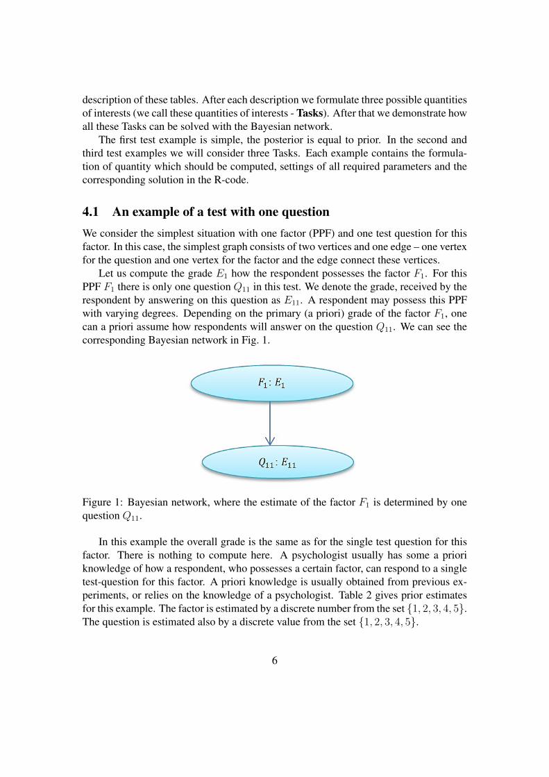
4.1 An example of a test with one questionWe consider the simplest situation with one factor (PPF) and one test question for thisfactor. In this case, the simplest graph consists of two vertices and one edge – one vertexfor the question and one vertex for the factor and the edge connect these vertices.

Let us compute the grade E1 how the respondent possesses the factor F1. For thisPPF F1 there is only one question Q11 in this test. We denote the grade, received by therespondent by answering on this question as E11. A respondent may possess this PPFwith varying degrees. Depending on the primary (a priori) grade of the factor F1, onecan a priori assume how respondents will answer on the question Q11. We can see thecorresponding Bayesian network in Fig. 1.

Figure 1: Bayesian network, where the estimate of the factor F1 is determined by onequestion Q11.

In this example the overall grade is the same as for the single test question for thisfactor. There is nothing to compute here. A psychologist usually has some a prioriknowledge of how a respondent, who possesses a certain factor, can respond to a singletest-question for this factor. A priori knowledge is usually obtained from previous ex-periments, or relies on the knowledge of a psychologist. Table 2 gives prior estimatesfor this example. The factor is estimated by a discrete number from the set {1, 2, 3, 4, 5}.The question is estimated also by a discrete value from the set {1, 2, 3, 4, 5}.

6

Table 2: A priori estimates for the test example from Section 4.1, where the overallgrade of the factor F1 is determined by one question Q11.

One can interpret values from Table 2 in the following way. A psychologist thinksthat

1. 70% of respondents, who do not possess the factor F1 (E1 = 0) will answer onthe question Q11 with grade E11 = 1.

2. only 20% of respondents, who possesses the factor F1 with grade (E1 = 3) willanswer the question Q11 with grade E11 = 5.

3. only 2% of respondents, who do not possess the factor F1 (E1 = 0) will answerthe question Q11 with grade E11 = 5.

This example is simple, the posterior probabilities are equal to prior probabilities.Table 2 gives us all necessary information. The situation becomes more complicated ifthere are several questions.

4.2 An example of a test with two questionsWe increase the complexity of the example from Section 4.1, namely, we consider twoquestions in the test. The PPF factor is estimated on a two-point scale. The question isestimated on a five-point scale. Therefore, the graph consists of 3 vertices and 2 edges(Murrell 2006). One can see the corresponding Bayesian network in Fig. 2.

Let us build the estimate E1 of F1. For this factor there are two questions Q11 andQ12 in the test. We denote these estimates of questions by E11 and E12 respectively.Table 3 gives prior estimates for this example.

One can interpret the values from Table 3 in the following way. A psychologistthinks that

1. 60% of respondents, who does not possess the factor F1 will answer the questionQ12 with grade E12 = 1.

7

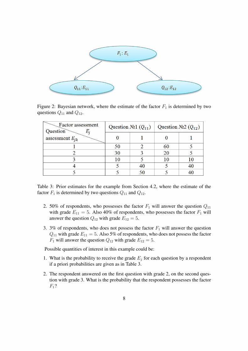
Figure 2: Bayesian network, where the estimate of the factor F1 is determined by twoquestions Q11 and Q12.

Table 3: Prior estimates for the example from Section 4.2, where the estimate of thefactor F1 is determined by two questions Q11 and Q12.

2. 50% of respondents, who possesses the factor F1 will answer the question Q11

with grade E11 = 5. Also 40% of respondents, who possesses the factor F1 willanswer the question Q12 with grade E12 = 5.

3. 3% of respondents, who does not possess the factor F1 will answer the questionQ11 with grade E11 = 5. Also 5% of respondents, who does not possess the factorF1 will answer the question Q12 with grade E12 = 5.

Possible quantities of interest in this example could be:

1. What is the probability to receive the grade Ej for each question by a respondentif a priori probabilities are given as in Table 3.

2. The respondent answered on the first question with grade 2, on the second ques-tion with grade 3. What is the probability that the respondent possesses the factorF1?

8

3. The respondent answered on the first question with grade 3. What is the prob-ability that the respondent will answer on the second question with grades 4 or5?

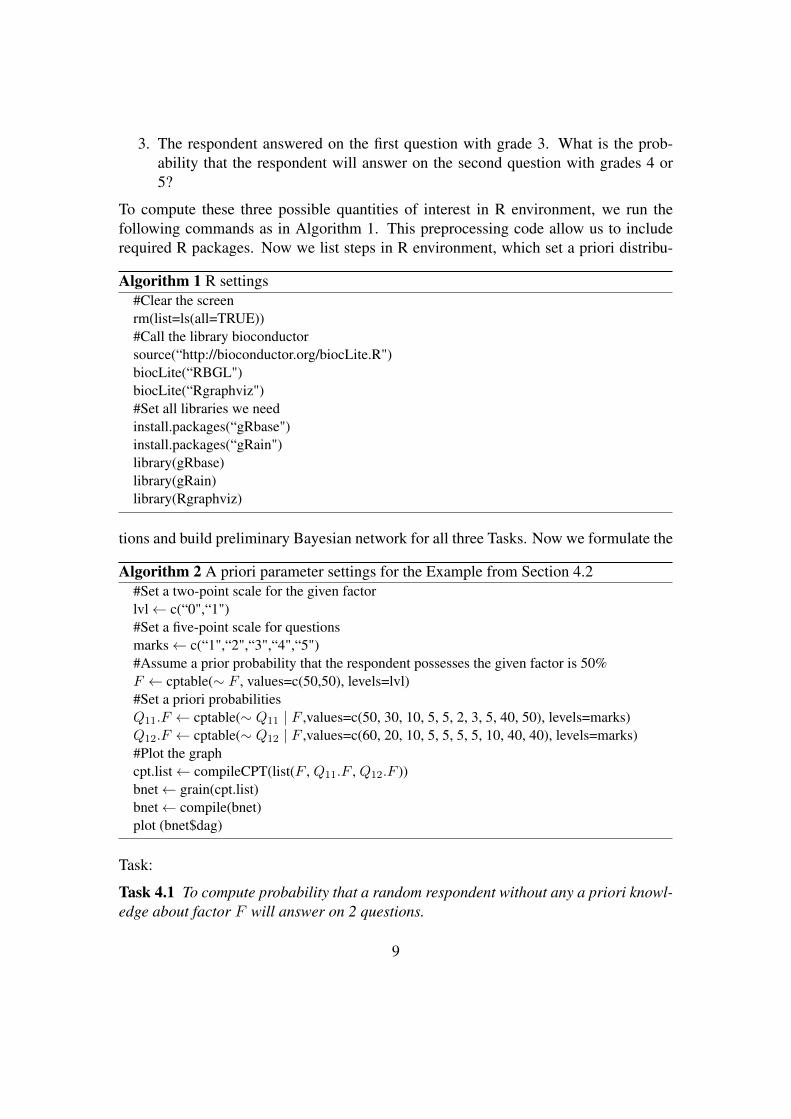
To compute these three possible quantities of interest in R environment, we run thefollowing commands as in Algorithm 1. This preprocessing code allow us to includerequired R packages. Now we list steps in R environment, which set a priori distribu-

Algorithm 1 R settings#Clear the screenrm(list=ls(all=TRUE))#Call the library bioconductorsource(“http://bioconductor.org/biocLite.R")biocLite(“RBGL")biocLite(“Rgraphviz")#Set all libraries we needinstall.packages(“gRbase")install.packages(“gRain")library(gRbase)library(gRain)library(Rgraphviz)

tions and build preliminary Bayesian network for all three Tasks. Now we formulate the

Algorithm 2 A priori parameter settings for the Example from Section 4.2#Set a two-point scale for the given factorlvl← c(“0",“1")#Set a five-point scale for questionsmarks← c(“1",“2",“3",“4",“5")#Assume a prior probability that the respondent possesses the given factor is 50%F ← cptable(∼ F , values=c(50,50), levels=lvl)#Set a priori probabilitiesQ11.F ← cptable(∼ Q11 | F ,values=c(50, 30, 10, 5, 5, 2, 3, 5, 40, 50), levels=marks)Q12.F ← cptable(∼ Q12 | F ,values=c(60, 20, 10, 5, 5, 5, 5, 10, 40, 40), levels=marks)#Plot the graphcpt.list← compileCPT(list(F , Q11.F , Q12.F ))bnet← grain(cpt.list)bnet← compile(bnet)plot (bnet$dag)

Task:

Task 4.1 To compute probability that a random respondent without any a priori knowl-edge about factor F will answer on 2 questions.

9

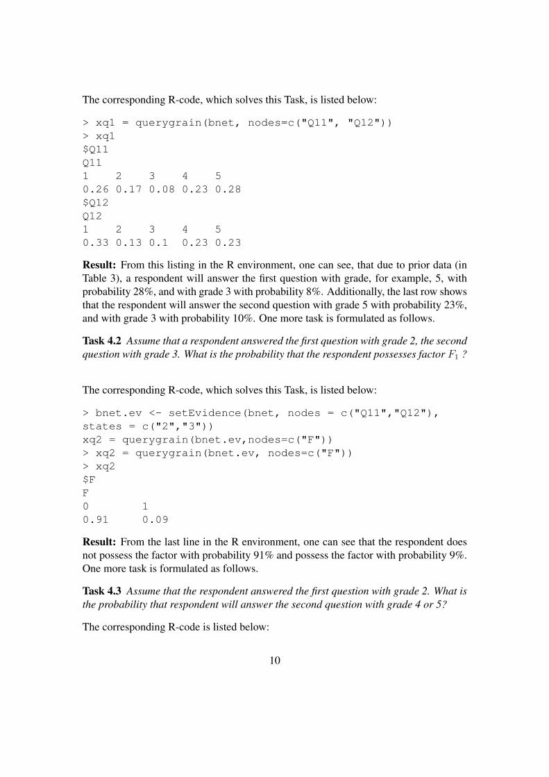
The corresponding R-code, which solves this Task, is listed below:

> xq1 = querygrain(bnet, nodes=c("Q11", "Q12"))> xq1$Q11Q111 2 3 4 50.26 0.17 0.08 0.23 0.28$Q12Q121 2 3 4 50.33 0.13 0.1 0.23 0.23

Result: From this listing in the R environment, one can see, that due to prior data (inTable 3), a respondent will answer the first question with grade, for example, 5, withprobability 28%, and with grade 3 with probability 8%. Additionally, the last row showsthat the respondent will answer the second question with grade 5 with probability 23%,and with grade 3 with probability 10%. One more task is formulated as follows.

Task 4.2 Assume that a respondent answered the first question with grade 2, the secondquestion with grade 3. What is the probability that the respondent possesses factor F1 ?

The corresponding R-code, which solves this Task, is listed below:

> bnet.ev <- setEvidence(bnet, nodes = c("Q11","Q12"),states = c("2","3"))xq2 = querygrain(bnet.ev,nodes=c("F"))> xq2 = querygrain(bnet.ev, nodes=c("F"))> xq2$FF0 10.91 0.09

Result: From the last line in the R environment, one can see that the respondent doesnot possess the factor with probability 91% and possess the factor with probability 9%.One more task is formulated as follows.

Task 4.3 Assume that the respondent answered the first question with grade 2. What isthe probability that respondent will answer the second question with grade 4 or 5?

The corresponding R-code is listed below:

10

> bnet.ev <- setEvidence(bnet, nodes = c("Q11"), states = c("3"))> xq2 = querygrain(bnet.ev, nodes=c("Q12"))> xq2$Q12Q121 2 3 4 50.42 0.15 0.1 0.17 0.17

Result: Respondent will answer the second question with grade 4 or 5 with probability17%+17%=34%.

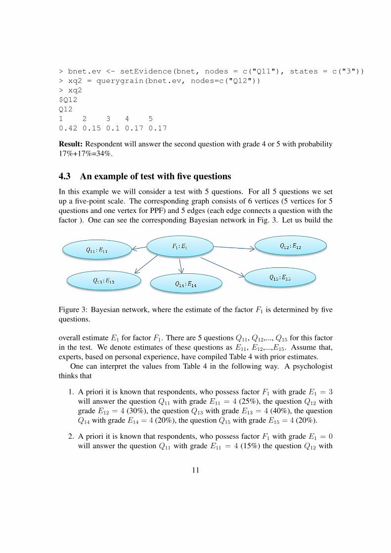
4.3 An example of test with five questionsIn this example we will consider a test with 5 questions. For all 5 questions we setup a five-point scale. The corresponding graph consists of 6 vertices (5 vertices for 5questions and one vertex for PPF) and 5 edges (each edge connects a question with thefactor ). One can see the corresponding Bayesian network in Fig. 3. Let us build the

Figure 3: Bayesian network, where the estimate of the factor F1 is determined by fivequestions.

overall estimate E1 for factor F1. There are 5 questions Q11, Q12,..., Q15 for this factorin the test. We denote estimates of these questions as E11, E12,...,E15. Assume that,experts, based on personal experience, have compiled Table 4 with prior estimates.

One can interpret the values from Table 4 in the following way. A psychologistthinks that

1. A priori it is known that respondents, who possess factor F1 with grade E1 = 3will answer the question Q11 with grade E11 = 4 (25%), the question Q12 withgrade E12 = 4 (30%), the question Q13 with grade E13 = 4 (40%), the questionQ14 with grade E14 = 4 (20%), the question Q15 with grade E15 = 4 (20%).

2. A priori it is known that respondents, who possess factor F1 with grade E1 = 0will answer the question Q11 with grade E11 = 4 (15%) the question Q12 with

11

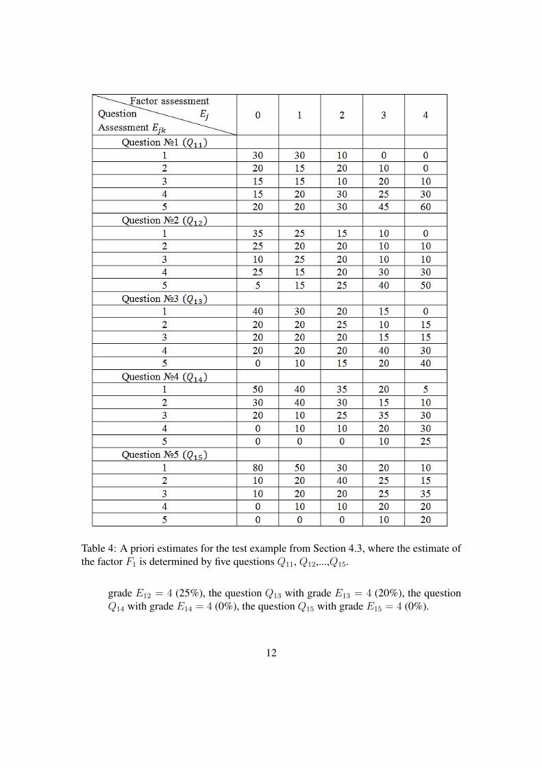
Table 4: A priori estimates for the test example from Section 4.3, where the estimate ofthe factor F1 is determined by five questions Q11, Q12,...,Q15.

grade E12 = 4 (25%), the question Q13 with grade E13 = 4 (20%), the questionQ14 with grade E14 = 4 (0%), the question Q15 with grade E15 = 4 (0%).

12

3. A priori it is known that respondents, who possess factor F1 with grade E1 = 4will answer the question Q11 with grade E11 = 3 (10%), the question Q12 withgrade E12 = 3 (10%), the question Q13 with grade E13 = 3 (15%), the questionQ14 with grade E14 = 3 (30%), the question Q15 with grade E15 = 3 (35%).

Possible quantities of interest here could be:

1. What is the probability that a respondent will answer all 5 questions with grade5?

2. The respondent answered the first question with grade 5, the second and the thirdquestions with grade 4. What is the probability that the respondent has the factorF1 with grade not less than 3?

3. The respondent answered the first question with grade 5, the second and thirdquestions with grade 3. What is the probability that the respondent will answerthe fourth and fifth questions with grades not less than 4?

The program code in R (Chambers 2008), computing quantities of interest, listedabove, is the following. The setting commands for R are omitted for brevity.

Task 4.4 Compute the probabilities that a respondent with no a priori information willanswer all 5 questions.

The corresponding R-code, which solves this Task, is listed below:

> xq1 = querygrain(bnet, nodes=c("Q11","Q12","Q13","Q14","Q15"))> xq1$Q11Q111 2 3 4 50.14 0.13 0.14 0.24 0.35$Q12Q121 2 3 4 50.17 0.17 0.15 0.24 0.27$Q13Q131 2 3 4 50.21 0.18 0.18 0.26 0.17$Q14Q141 2 3 4 5

13

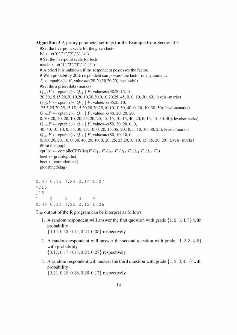
Algorithm 3 A priory parameter settings for the Example from Section 4.3#Set the five-point scale for the given factorlvl← c("0","1","2","3","4")# Set the five-point scale for testsmarks← c("1","2","3","4","5")# A priori it is unknown if the respondent possesses the factor.# With probability 20% respondent can possess the factor in any amount.F ← cptable(∼ F , values=c(20,20,20,20,20),levels=lvl)#Set the a priori data (marks)Q11.F ← cptable(∼ Q11 | F , values=c(30,20,15,15,20,30,15,15,20,20,10,20,10,30,30,0,10,20,25, 45, 0, 0, 10, 30, 60), levels=marks)Q12.F ← cptable(∼ Q12 | F , values=c(35,25,10,25,5,25,20,25,15,15,15,20,20,20,25,10,10,10,30, 40, 0, 10, 10, 30, 50), levels=marks)Q13.F ← cptable(∼ Q13 | F , values=c(40, 20, 20, 20,0, 30, 20, 20, 20, 10, 20, 25, 20, 20, 15, 15, 10, 15, 40, 20, 0, 15, 15, 30, 40), levels=marks)Q14.F ← cptable(∼ Q14 | F , values=c(50, 30, 20, 0, 0,40, 40, 10, 10, 0, 35, 30, 25, 10, 0, 20, 15, 35, 20,10, 5, 10, 30, 30, 25), levels=marks)Q15.F ← cptable(∼ Q15 | F , values=c(80, 10, 10, 0,0, 50, 20, 20, 10, 0, 30, 40, 20, 10, 0, 20, 25, 25,20,10, 10, 15, 35, 20, 20), levels=marks)#Plot the graphcpt.list← compileCPT(list(F,Q11.F,Q12.F,Q13.F,Q14.F,Q15.F ))bnet← grain(cpt.list)bnet← compile(bnet)plot (bnet$dag)

0.30 0.25 0.24 0.14 0.07$Q15Q151 2 3 4 50.38 0.22 0.22 0.12 0.06

The output of the R program can be interpret as follows

1. A random respondent will answer the first question with grade {1, 2, 3, 4, 5} withprobability{0.14, 0.13, 0.14, 0.24, 0.35} respectively.

2. A random respondent will answer the second question with grade {1, 2, 3, 4, 5}with probability{0.17, 0.17, 0.15, 0.24, 0.27} respectively.

3. A random respondent will answer the third question with grade {1, 2, 3, 4, 5}withprobability{0.21, 0.18, 0.18, 0.26, 0.17} respectively.

14

4. A random respondent will answer the fourth question with grade {1, 2, 3, 4, 5}with probability{0.30, 0.25, 0.24, 0.14, 0.07} respectively.

5. A random respondent will answer the fifth question with grade {1, 2, 3, 4, 5} withprobability{0.38, 0.22, 0.22, 0.12, 0.06} respectively.

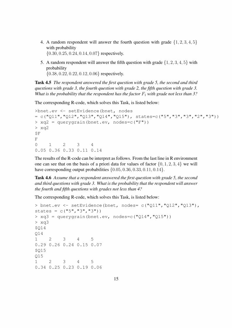
Task 4.5 The respondent answered the first question with grade 5, the second and thirdquestions with grade 3, the fourth question with grade 2, the fifth question with grade 3.What is the probability that the respondent has the factor F1 with grade not less than 3?

The corresponding R-code, which solves this Task, is listed below:

>bnet.ev <- setEvidence(bnet, nodes= c("Q11","Q12","Q13","Q14","Q15"), states=c("5","3","3","2","3"))> xq2 = querygrain(bnet.ev, nodes=c("F"))> xq2$FF0 1 2 3 40.05 0.36 0.33 0.11 0.14

The results of the R-code can be interpret as follows. From the last line in R environmentone can see that on the basis of a priori data for values of factor {0, 1, 2, 3, 4} we willhave corresponding output probabilities {0.05, 0.36, 0.33, 0.11, 0.14}.

Task 4.6 Assume that a respondent answered the first question with grade 5, the secondand third questions with grade 3. What is the probability that the respondent will answerthe fourth and fifth questions with grades not less than 4?

The corresponding R-code, which solves this Task, is listed below:

> bnet.ev <- setEvidence(bnet, nodes= c("Q11","Q12","Q13"),states = c("5","3","3"))> xq3 = querygrain(bnet.ev, nodes=c("Q14","Q15"))> xq3$Q14Q141 2 3 4 50.29 0.26 0.24 0.15 0.07$Q15Q151 2 3 4 50.34 0.25 0.23 0.19 0.06

15

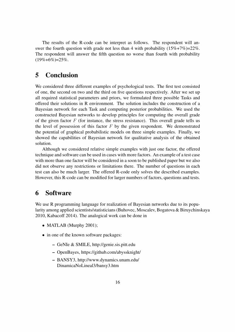
The results of the R-code can be interpret as follows. The respondent will an-swer the fourth question with grade not less than 4 with probability (15%+7%)=22%.The respondent will answer the fifth question no worse than fourth with probability(19%+6%)=25%.

5 ConclusionWe considered three different examples of psychological tests. The first test consistedof one, the second on two and the third on five questions respectively. After we set upall required statistical parameters and priors, we formulated three possible Tasks andoffered their solutions in R environment. The solution includes the construction of aBayesian network for each Task and computing posterior probabilities. We used theconstructed Bayesian networks to develop principles for computing the overall gradeof the given factor F (for instance, the stress resistance). This overall grade tells usthe level of possession of this factor F by the given respondent. We demonstratedthe potential of graphical probabilistic models on three simple examples. Finally, weshowed the capabilities of Bayesian network for qualitative analysis of the obtainedsolution.

Although we considered relative simple examples with just one factor, the offeredtechnique and software can be used in cases with more factors. An example of a test casewith more than one factor will be considered in a soon to be published paper but we alsodid not observe any restrictions or limitations there. The number of questions in eachtest can also be much larger. The offered R-code only solves the described examples.However, this R-code can be modified for larger numbers of factors, questions and tests.

6 SoftwareWe use R programming language for realization of Bayesian networks due to its popu-larity among applied scientists/statisticians (Buhovec, Moscalev, Bogatova & Biruychinskaya2010, Kabacoff 2014). The analogical work can be done in

• MATLAB (Murphy 2001);

• in one of the known software packages:

– GeNIe & SMILE, http://genie.sis.pitt.edu

– OpenBayes, https://github.com/abyssknight/

– BANSY3, http://www.dynamics.unam.edu/DinamicaNoLineal3/bansy3.htm

16

• in one of the commercial products: AgenaRisk Bayesian network tool, Bayesiannetwork application library, Bayesia, BNet.

6.1 ReproducibilityTo reproduce the presented results one can download the R-code from Dropboxhttps://www.dropbox.com/sh/t8cm12vv741a0h0/AABz_SwBEQ5mgKMyRAcl51mZa?dl=0.

AcknowledgmentThis work was supported by the Institute of Mathematics and Mathematical ModelingCS MES Republic of Kazakhstan and by the Ministry of Education and Science ofKazakhstan, (grant number is 4085/GF4, 0115RK00640).

Additionally, we would like to express our enormous gratitude to Prof. MaksatKalimoldayev, Academic member of the National Academy of Sciences, the head ofInstitute of Information and Computational Technologies CS MES Republic of Kaza-khstan for his organizational assistance, valuable comments and financial support.

ReferencesAlbert, J. (2009). Bayesian Computation with R, Springer.

Baizhanov, B. & Litvinenko, N. (2014). Parallel algorithms for clusterization problemswith using the gpu, CUDA ALMANAKH, NVIDIA p. 8.

Ben-Gal, I. (2008). Bayesian Networks, John Wiley & Sons, Ltd.URL: http://dx.doi.org/10.1002/9780470061572.eqr089

Berikov, V. B., Lbov, G. S. & Litvinenko, A. G. (2004). Discrete recognition problemwith a randomized decision function, PATTERN RECOGNITION AND IMAGEANALYSIS C/C OF RASPOZNAVANIYE OBRAZOV I ANALIZ IZOBRAZHENII.14(2): 211–221.

Berikov, V. & Litvinenko, A. (2003a). The influence of prior knowledge on the expectedperformance of a classifier, Pattern recognition letters 24(15): 2537–2548.

Berikov, V. & Litvinenko, A. (2003b). Methods for statistical data analysis with decisiontrees, Novosibirsk, Sobolev Institute of Mathematics .

Buhovec, A., Moscalev, P., Bogatova, V. & Biruychinskaya, T. (2010). Statistical dataanalysis in R, VGAU, Voronezh.

17

Chambers, J. (2008). Software for Data Analysis: Programming with R, Springer, NewYork.

Kabacoff, R. (2014). R in Action, DMK Press, MoscowL.

Litvinenko, N. (2016a). Integration of r software environment in c# software environ-ment, News of the National Academy of Sciences of the RK, Physico-mathematicalseries 2: 123–127.

Litvinenko, N. (2016b). Questionnaires recognition during social research, News of theNational Academy of Sciences of the RK, Physico-mathematical series 3: 77–82.

Matthies, H. G., Litvinenko, A., Pajonk, O., Rosic, B. V. & Zander, E. (2012). Paramet-ric and uncertainty computations with tensor product representations, UncertaintyQuantification in Scientific Computing, Vol. 377 of IFIP Advances in Informationand Communication Technology, Springer Berlin Heidelberg, pp. 139–150.

Matthies, H. G., Litvinenko, A., Rosic, B. & Zander, E. (2016). Bayesian pa-rameter estimation via filtering and functional approximations, arXiv preprintarXiv:1611.09293 .

Matthies, H. G., Zander, E., Rosic, B. V. & Litvinenko, A. (2016). Parameter estima-tion via conditional expectation: a Bayesian inversion, Advanced modeling andsimulation in engineering sciences 3(1): 24.

Matthies, H., Zander, E., Pajonk, O., Rosic, B. & Litvinenko, A. (2016). Inverse prob-lems in a Bayesian setting, Computational Methods for Solids and Fluids Mul-tiscale Analysis, Probability Aspects and Model Reduction Editors: Ibrahimbe-govic, Adnan (Ed.), ISSN: 1871-3033, Springer, pp. 245–286.

Murphy, K. (2001). The bayes net toolbox for matlab, Computing science and statisticspp. 1024–1034.

Murrell, P. (2006). R Graphics, Chapman & Hall/CRC, Boca Raton, FL.

Pajonk, O., Rosic, B. V., Litvinenko, A. & Matthies, H. G. (2012). A deterministic filterfor non-gaussian Bayesian estimation – applications to dynamical system estima-tion with noisy measurements, Physica D: Nonlinear Phenomena 241(7): 775–788.

Pourret, O., Naim, P. & Marcot, B. (2008). Bayesian Networks: A Practical Guide toApplications, John Wiley and Sons, Ltd.

18

Rosic, B., Kucerová, A., Sýkora, J., Pajonk, O., Litvinenko, A. & Matthies, H. G.(2013). Parameter identification in a probabilistic setting, Engineering Structures50(0): 179 – 196. Engineering Structures: Modelling and Computations (specialissue IASS-IACM 2012).URL: http://www.sciencedirect.com/science/article/pii/S0141029612006426

Rosic, B. V., Kucerová, A., Sykora, J., Pajonk, O., Litvinenko, A. & Matthies, H. G.(2013). Parameter identification in a probabilistic setting, Engineering Structures50: 179–196.

Rosic, B. V., Litvinenko, A., Pajonk, O. & Matthies, H. G. (2011). Direct Bayesianupdate of polynomial chaos representations, Journal of Computational Physics .

Rosic, B. V., Litvinenko, A., Pajonk, O. & Matthies, H. G. (2012). Sampling-free linearBayesian update of polynomial chaos representations, Journal of ComputationalPhysics 231(17): 5761–5787.

Tulupyev, A., Nikolenko, S. & Sirotkin, A. (2006). Bayesian Networks. A probabilisticlogic approach, Nauka, St.Petersburg.

19

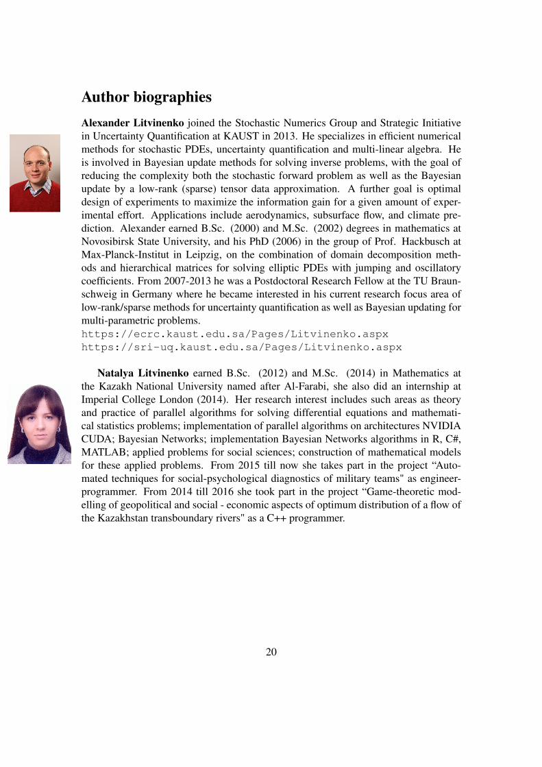
Author biographiesAlexander Litvinenko joined the Stochastic Numerics Group and Strategic Initiativein Uncertainty Quantification at KAUST in 2013. He specializes in efficient numericalmethods for stochastic PDEs, uncertainty quantification and multi-linear algebra. Heis involved in Bayesian update methods for solving inverse problems, with the goal ofreducing the complexity both the stochastic forward problem as well as the Bayesianupdate by a low-rank (sparse) tensor data approximation. A further goal is optimaldesign of experiments to maximize the information gain for a given amount of exper-imental effort. Applications include aerodynamics, subsurface flow, and climate pre-diction. Alexander earned B.Sc. (2000) and M.Sc. (2002) degrees in mathematics atNovosibirsk State University, and his PhD (2006) in the group of Prof. Hackbusch atMax-Planck-Institut in Leipzig, on the combination of domain decomposition meth-ods and hierarchical matrices for solving elliptic PDEs with jumping and oscillatorycoefficients. From 2007-2013 he was a Postdoctoral Research Fellow at the TU Braun-schweig in Germany where he became interested in his current research focus area oflow-rank/sparse methods for uncertainty quantification as well as Bayesian updating formulti-parametric problems.https://ecrc.kaust.edu.sa/Pages/Litvinenko.aspxhttps://sri-uq.kaust.edu.sa/Pages/Litvinenko.aspx

Natalya Litvinenko earned B.Sc. (2012) and M.Sc. (2014) in Mathematics atthe Kazakh National University named after Al-Farabi, she also did an internship atImperial College London (2014). Her research interest includes such areas as theoryand practice of parallel algorithms for solving differential equations and mathemati-cal statistics problems; implementation of parallel algorithms on architectures NVIDIACUDA; Bayesian Networks; implementation Bayesian Networks algorithms in R, C#,MATLAB; applied problems for social sciences; construction of mathematical modelsfor these applied problems. From 2015 till now she takes part in the project “Auto-mated techniques for social-psychological diagnostics of military teams" as engineer-programmer. From 2014 till 2016 she took part in the project “Game-theoretic mod-elling of geopolitical and social - economic aspects of optimum distribution of a flow ofthe Kazakhstan transboundary rivers" as a C++ programmer.

20