Application of Anisotropic Rock Physics Modeling in Integrated Interpretation of Seismic and CSEM Data Michelle Ellis(1), Franklin Ruiz(1), Sriram Nanduri(1), Robert Keirstead(1), Ilgar Azizov(1), Michael Frenkel(1), and Lucy MacGregor(1). (1)

RSI. ABSTRACT

Elastic and electrical anisotropy in rocks exists on a large range of length-scales. It is important to understand elastic anisotropy to avoid: misplacing seismic reflectors; incorrect well-ties; inaccurate AVO interpretation; and inaccurate seismic inversion. Similar is true for electrical anisotropy when: interpreting CSEM and well-log data; quantifying resistivity anisotropy; using log data to ground truth CSEM inversion data; estimating hydrocarbon saturations, and using log data to build realistic starting models for CSEM inversion. In this study a workflow is presented combining rock physics modelling, upscaling, and feasibility studies to jointly interpret co-located elastic and electric properties at a given site. Rock physics models are developed which calculate elastic and electrical anisotropy from the volumetric fractions of solids and fluids in the rock, and the microstructural information within the rock. To upscale the geophysical properties the subsurface strata is treated as a stack of fine isotropic and/or transverse isotropic layers, each with its symmetry axis normal to the bedding plane. Seismic feasibility is accomplished using synthetic seismograms and CSEM feasibility is achieved by calculating the synthetic amplitudes. Case studies are presented using the workflow. KEY WORDS: Anisotropy, rock physics, elastic, electrical, upscaling, CSEM. INTRODUCTION Typically, elastic wave travel times are measured at three different timescales: seismic (~40 Hz), well log (~10 kHz), and laboratory (~1 MHz). Resistivity is also typically measured at different scales, 2-1000 Hz in the laboratory, >20 KHz in the well log and ~1 Hz for Controlled-Source Electromagnetic (CSEM) surveying. Even though, at seismic and CSEM scales, a large percentage of sedimentary rocks are anisotropic, most data processing workflows assume that the medium is isotropic. Shales, which comprise about 75% of the clastic fill of sedimentary basins (Jones and Wang, 1981), tend to exhibit high levels of elastic and electrical anisotropy (Ellis et al., 2010). The degree of anisotropy depends on the rock constituents volumetric fractions and on the size and orientation of rock fabric heterogeneities compared to the length scale of measurement. Some of the dominant shale fabric

features responsible for anisotropy are: a) bedding, b) alignments of silt grains, flaky flocculated clay particles, and layers of organic material, and c) alignment of fracture sets with different orientations.

Overlooking elastic anisotropy leads to the misplacing of seismic reflectors, unfocused seismic imaging, incorrect well-ties, and inaccurate quantitative seismic interpretation. Disregarding resistivity anisotropy may lead to misleading CSEM survey feasibility studies, inaccurate CSEM data inversion, inaccurate estimations of hydrocarbon saturations and difficultly when using well logs to ground truth CSEM inversions. For accurate integrated quantitative seismic and CSEM interpretation, it is necessary to develop techniques to estimate all the unmeasured elements of the elastic and resistivity tensors from the commonly measured elements. This can be done using rock physics models based on density, sonic and resistivity (horizontal) log data, which are consistent with the available microstructural information.

In this study a joint seismic and electrical workflow is presented which uses rock physics models to estimate the unknown elements of the rock elastic and resistivity tensors. These physical properties, which are measured on the well-log scale are upscaled and then used for seismic and CSEM feasibility studies. The importance of understanding anisotropy and its effects on seismic and CSEM data is demonstrated using two case studies. INTEGRATED SEISMIC AND CSEM DATA INTERPRETATION WORKFLOW Figure 1 shows an integrated seismic and CSEM feasibility workflow for anisotropic media. It is important that the electrical and seismic work is consistent and done in parallel steps throughout the workflow. Inputs into the elastic and electrical models (such as mineral volume) should be the same or equivalent. The main steps of the workflow are: Step 1: Geophysical Well-Log Analysis (GWLA) –

This is required to build a good and consistent well-log data set for the rock physics modelling. In this step, we estimate volumetric fractions of solid and fluid constituents.

Step 2: Estimate elastic and electrical properties at well-log scale, from well-log measurements, and the rock physics models described below.

Step 3: Fluid substitution is conducted for different fluid saturation scenarios. Gassmann’s fluid

Proceedings of the 10th SEGJ International Symposium, 2011 453

Dow

nloa

ded

07/2

5/17

to 7

2.26

.15.

23. R

edis

trib

utio

n su

bjec

t to

SEG

lice

nse

or c

opyr

ight

; see

Ter

ms

of U

se a

t http

://lib

rary

.seg

.org

/

substitution is used for the elastic data and Archie’s equation is used for resistivity data.

Step 4: Upscaling - The well-log-scale elastic properties are upscaled to seismic wavelengths using Backus Averaging (BA). The electrical properties are upscaled by assuming each layer is a resistor and averaged using an in-series or parallel resistor network configuration.

Step 5: Feasibility studies: The objective of a seismic feasibility study is to calculate the effect of variations in reservoir properties and physical conditions on synthetic seismograms (e.g., seismic waveform, travel times, wavefront, wavefield, AVO). CSEM feasibility is achieved by calculating the synthetic amplitude responses for both the wet and hydrocarbon charged models over a range of frequencies and source-receiver offsets. The normalized difference is then calculated between the two models and assessed to determine whether the target reservoir is resolvable using CSEM.

Step 6: Inversion of seismic and CSEM synthetic data: Whereas it is important to demonstrate that seismic and CSEM methods are sensitive to changes in rock and fluid properties, it is also critical to assess the accuracy with which quantitative information on earth lithology and fluid properties can be determined from survey data.

Step 7: Integrated interpretation of results: This is done to fully describe the site in both seismic and electrical terms. Jointly interpreting the results allows a more informed review of the type of geophysical survey is suitable for this particular case.

ROCK PHYSICS MODELLING

Elastic The elastic properties of Vertical Transverse Isotropic (VTI) shale is estimated using a hybrid rock physics model. The model assumes that the solid shale matrix is isotropic, with all solid constituent grains randomly oriented and distributed through the host. The total pore space is divided into two spaces: the stiff and soft pore space. The stiff pores have an aspect ratio of 1 (spheres) while the soft pores have variable aspect ratios (Ruiz and Cheng, 2010). The soft pores are assumed to be preferentially oriented in the horizontal direction. The model estimates the effective elastic moduli of an isotropic rock matrix with embedded stiff fluid-saturated pores, using the self-consistent approximation (Berryman, 1995). Then the Hudson’s model (Hudson, 1980) is used to account for the embedded crack-like fluid saturated pores in the effective medium. The unknown elements of the rock elastic tensor are estimated by searching for the required soft porosity that minimizes the difference between the measured vertical sonic S- and P-wave velocities, and the theoretical vertical velocities. Electrical The electrical Differential Effective Medium (DEM) model (Berryman, 1995) models anisotropy by aligning inclusions within a host medium. The DEM method models an effective medium by starting with a medium composed of a single material, to which inclusions with a known geometric shape are incrementally added. The DEM method preserves the microstructure of the starting medium (Sheng, 1990). It follows that if the starting medium is brine it will remain interconnected at all porosities and all other components will remain isolated. To determine vertical and horizontal resistivity from a well log it is assumed that the grains are fully aligned. The horizontal resistivity is calculated from the porosity and the mineral volumes at every measurement point throughout the sediment column. The DEM model is adjusted so that the calculated horizontal resistivity trend matches the log measured resistivity trend. Once this is done, the same model is used to calculate the corresponding vertical resistivities. CASE STUDY 1: FORT WORTH BASIN (BARNETT SHALE) In this example well data from the Barnett shale in the Fort Worth Basin, in Texas, USA is used. The well logs show physical properties (e.g., velocities, density, resistivity, porosity, mineralogy, fluids) change over small intervals, which is indicative of fine heterogeneities in the subsurface formations. The unknown elements of the elastic tensor, at well-log scale, are estimated using the rock physics method above (step 2). At well log scale, only anisotropy due to horizontally oriented hydrocarbon generated microcracks (soft pores) is considered. After upscaling (step 4), the Barnett Shale interval shows

Figure 1. Flowchart of integrated seismic and CSEMfeasibility study using anisotropic models.

Proceedings of the 10th SEGJ International Symposium, 2011454

Dow

nloa

ded

07/2

5/17

to 7

2.26

.15.

23. R

edis

trib

utio

n su

bjec

t to

SEG

lice

nse

or c

opyr

ight

; see

Ter

ms

of U

se a

t http

://lib

rary

.seg

.org

/

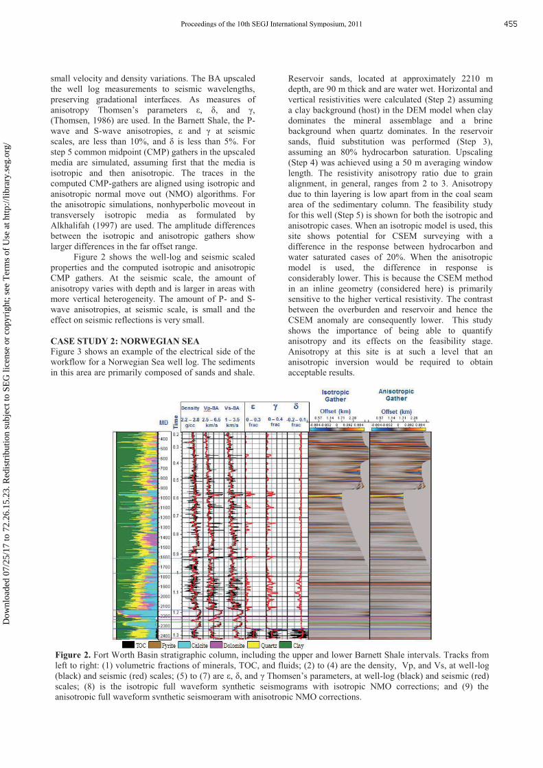
small velocity and density variations. The BA upscaled the well log measurements to seismic wavelengths, preserving gradational interfaces. As measures of anisotropy Thomsen’s parameters ε, δ, and γ, (Thomsen, 1986) are used. In the Barnett Shale, the P-wave and S-wave anisotropies, ε and γ at seismic scales, are less than 10%, and δ is less than 5%. For step 5 common midpoint (CMP) gathers in the upscaled media are simulated, assuming first that the media is isotropic and then anisotropic. The traces in the computed CMP-gathers are aligned using isotropic and anisotropic normal move out (NMO) algorithms. For the anisotropic simulations, nonhyperbolic moveout in transversely isotropic media as formulated by Alkhalifah (1997) are used. The amplitude differences between the isotropic and anisotropic gathers show larger differences in the far offset range. Figure 2 shows the well-log and seismic scaled properties and the computed isotropic and anisotropic CMP gathers. At the seismic scale, the amount of anisotropy varies with depth and is larger in areas with more vertical heterogeneity. The amount of P- and S-wave anisotropies, at seismic scale, is small and the effect on seismic reflections is very small. CASE STUDY 2: NORWEGIAN SEA Figure 3 shows an example of the electrical side of the workflow for a Norwegian Sea well log. The sediments in this area are primarily composed of sands and shale.

Reservoir sands, located at approximately 2210 m depth, are 90 m thick and are water wet. Horizontal and vertical resistivities were calculated (Step 2) assuming a clay background (host) in the DEM model when clay dominates the mineral assemblage and a brine background when quartz dominates. In the reservoir sands, fluid substitution was performed (Step 3), assuming an 80% hydrocarbon saturation. Upscaling (Step 4) was achieved using a 50 m averaging window length. The resistivity anisotropy ratio due to grain alignment, in general, ranges from 2 to 3. Anisotropy due to thin layering is low apart from in the coal seam area of the sedimentary column. The feasibility study for this well (Step 5) is shown for both the isotropic and anisotropic cases. When an isotropic model is used, this site shows potential for CSEM surveying with a difference in the response between hydrocarbon and water saturated cases of 20%. When the anisotropic model is used, the difference in response is considerably lower. This is because the CSEM method in an inline geometry (considered here) is primarily sensitive to the higher vertical resistivity. The contrast between the overburden and reservoir and hence the CSEM anomaly are consequently lower. This study shows the importance of being able to quantify anisotropy and its effects on the feasibility stage. Anisotropy at this site is at such a level that an anisotropic inversion would be required to obtain acceptable results.

Figure 2. Fort Worth Basin stratigraphic column, including the upper and lower Barnett Shale intervals. Tracks from left to right: (1) volumetric fractions of minerals, TOC, and fluids; (2) to (4) are the density, Vp, and Vs, at well-log (black) and seismic (red) scales; (5) to (7) are ε, δ, and γ Thomsen’s parameters, at well-log (black) and seismic (red) scales; (8) is the isotropic full waveform synthetic seismograms with isotropic NMO corrections; and (9) the anisotropic full waveform synthetic seismogram with anisotropic NMO corrections.

Proceedings of the 10th SEGJ International Symposium, 2011 455

Dow

nloa

ded

07/2

5/17

to 7

2.26

.15.

23. R

edis

trib

utio

n su

bjec

t to

SEG

lice

nse

or c

opyr

ight

; see

Ter

ms

of U

se a

t http

://lib

rary

.seg

.org

/

CONCLUSIONS Seismic and CSEM methods evaluate the same strata using fundamentally different techniques. Seismic surveying produces is sensitive to geological structure whereas CSEM provides information on the fluid properties of the rock. The advantages of the rock physics analysis presented here to calculate and upscale anisotropic elastic properties include: proper treatment of seismic anisotropy; avoiding misplacing seismic reflectors; better well ties; improved AVA interpretation and more reliable seismic inversion. It is important to assess resistivity anisotropy when interpreting CSEM and log data to perform reliable CSEM feasibility studies and build more realistic starting models for CSEM inversion and perform accurate CSEM inversion using additional information from log data. The workflow introduced in this paper demonstrates a systematic method of analysing elastic and electrical anisotropy. ACKNOWLEDGEMENTS The authors would like to thank DetNorske for providing field data, WISE consortium sponsors for valuable feedback and support, and C. Ramananjaona for performing 1D CSEM inversion.

REFERENCES

Alkhalifah, T., 1997, Velocity analysis using nonhyperbolic moveout in transversely isotropic media, Geophysics, 62, 1839–1854.

Berryman J. G., 1995. Mixture theories for rock properties. In AGU Handbook of Physical Constants, edited by T. J. Ahrens, AGU, New York, 205–228.

Ellis, M.H., Sinha, M.C., and Parr, R., 2010a, Role of fine-scale layering and grain alignment in the electrical anisotropy of marine sediments, First Break, 28 (9), 49-57.

Hudson, J.A., 1980, Overall properties of a cracked solid, Mathematical Proceedings of the Cambridge Philosophical Society, 88, 371-384.

Jones, L. and Wang, H. 1981, Ultrasonic velocities in Cretaceous shales from the Williston basin, Geophysics, 46, 288–297.

Ruiz F., and Cheng, A. 2010, A rock physics model for tight gas sand, The Leading Edge, 29, 1484-1489.

Sheng, P., 1990, Effective-medium theory of sedimentary rocks, Physical Review B, 41, 4507-4512.

Thomsen, L., 1986, Weak elastic anisotropy, Geophysics, 51, 1954–1966.

Figure 3. Electrical workflow for a Norwegian Sea well log. Numbers at the top of the figure refer to the workflow steps in Figure 1. Tracks from left to right: mineral composition of the sedimentary column; original log resistivities and horizontal and vertical resistivities calculated from the log; vertical and horizontal reistivties when the reservoir has been filled with 80% hydrocarbon; anisotropy determined from the log reistisvities, calculated resistivities and upscaled resistivities; upscaled resistivities; CSEM feasibility study using the resistivities from the fluid substitution; and 1D synthetic data anisotropic inversion results.

Proceedings of the 10th SEGJ International Symposium, 2011456

Dow

nloa

ded

07/2

5/17

to 7

2.26

.15.

23. R

edis

trib

utio

n su

bjec

t to

SEG

lice

nse

or c

opyr

ight

; see

Ter

ms

of U

se a

t http

://lib

rary

.seg

.org

/