Application of an Analytical Method to Locate a Mixing ... · PDF fileApplication of an...

Journal of Energy and Power Engineering 9 (2015) 91-101 doi: 10.17265/1934-8975/2015.01.011

Application of an Analytical Method to Locate a Mixing

Plane in a Supersonic Compressor

Emmanuel Benichou1 and Isabelle Trébinjac2

1. Turbomeca, Groupe SAFRAN, Bordes 64511, France

2. Laboratoire de Mécanique des Fluides et d’Acoustique, UMR CNRS 5509, Ecole Centrale de Lyon, Ecully Cedex 69134, France

Received: September 12, 2014 / Accepted: November 03, 2014 / Published: January 31, 2015. Abstract: In order to achieve greater pressure ratios, compressor designers have the opportunity to use transonic configurations. In the supersonic part of the incoming flow, shock waves appear in the front part of the blades and propagate in the upstream direction. In case of multiple blade rows, steady simulations have to impose an azimuthal averaging (mixing plane) which prevents these shock waves to extend upstream. In the present paper, several mixing plane locations are numerically tested and compared in a supersonic configuration. An analytical method is used to describe the shock pattern. It enables to take a critical look at the CFD (computational fluid dynamics) steady results. Based on this method, the shock losses are also evaluated. The good agreement between analytical and numerical values shows that this method can be useful to wisely forecast the mixing plane location and to evaluate the shift in performances due to the presence of the mixing plane. Key words: Supersonic compressor, shock wave, pressure loss, RANS, mixing plane.

Nomenclature

Symbol

P Static pressure

tP Stagnation pressure in the impeller frame

tP Circumferentially averaged stagnation pressure

t Circumferential pitch Density

V Velocity in the impeller frame

nV Normal velocity component

1 2,t tV V Tangential velocity components

r Radius a Speed of sound Perfect gas constant

Rotation speed

x0 Position of the bow shock on the profile symmetry axis

x, y Coordinates of a point in the profile frame

M Mach number

Corresponding author: Emmanuel Benichou, Ph.D. student,

research fields: aerodynamic instabilities in centrifugal compressors, including rotor-stator interactions and flow control issues using boundary layer aspiration. E-mail: [email protected].

µ Mach angle

Angle of the flow

Angle of the bow shock

eB Axial distance between points x0 and B

d Detachment distance of the shock wave

Pitchwise distance on which the flow is considered isentropic

θ Circumferential direction

K Total pressure loss coefficient

Subscript

B, C Relative to points B and C

1, 2 Calculated in Section 1 or Section 2

∞ Value of the quantity at infinite upstream

Exponent

* Value of the quantity at M = 1

1. Introduction

The need for compact, efficient high pressure ratio

compressors often results in high rotation speeds. In

some cases, the entry flow may therefore be supersonic

over the entire- or upper-span. The resulting physics of

the flow field in the entry zone can be complex because

D DAVID PUBLISHING

Application of an Analytical Method to Locate a Mixing Plane in a Supersonic Compressor

92

of the interaction between compression and expansion

waves [1-3]. Besides, shock waves propagating

upstream the blades are dissipative and must

necessarily be taken into account in the prediction of

the stage performances [4].

Current CFD (computational fluid dynamics) offers

three main categories for simulations: RANS

(Reynolds-averaged Navier-Stokes), LES (large eddy

simulation) and DNS (direct numerical simulation).

RANS simulations approximate the mean effect of

turbulence, while DNS enables a full resolution of the

Navier-Stokes equations, from the smallest turbulence

scale (Kolmogorov scale) up to the integral scale. LES

corresponds to a filtered DNS: only the largest

turbulence scales are resolved, the smallest ones being

modeled. The more turbulence scales are resolved, the

finer the mesh must be, and thus the more expensive

the simulation becomes.

In a current engine design process, only RANS

simulations can be carried out. This sort of simulation

is based on the Reynolds decomposition and turbulence

models are added to close the set of equations.

U-RANS (unsteady RANS) simulations are generally

not affordable in a conception approach, because of

their high CPU cost. That is why the only tool typically

available for designers today consists in steady RANS

simulations. In the case of multi-row turbomachinery,

these simulations rely most of the time on the use of

mixing planes, which average the data in the

circumferential direction, and thus do not let the

non-uniformities in the flow field transmit in the

upstream or downstream direction.

This article focuses on the entry zone of a supersonic

compressor. The filtration of the shock pattern

upstream the blades by the mixing plane raises the

issue of the mixing plane location. The present paper

compares numerically different locations to point out

the influence of the mixing plane on the flow field,

notably in terms of stagnation pressure change.

In a first part, the numerical results are qualitatively

analyzed and the role of the mixing plane is highlighted.

An analytical model is then used to reproduce the shape

of the shock waves at the leading edge of the blades.

Finally, a method is given that enables to judge the

reliability of steady simulations on supersonic

configurations.

2. Test Case and Numerical Procedure

The test case is a centrifugal unshrouded impeller

designed and built by Turbomeca. In the present study,

only the front part of it is concerned. There is therefore

no need giving the compressor geometry and

performance in this paper. Only one operating point is

examined, and it corresponds to the sonic blockage

region. The flow, supersonic over 60% of the span, is

examined at several section heights between h1 and h2

in Fig. 1.

A simulation performed without any mixing plane is

used as reference (Fig. 2a). In this one, the inlet block

is rotating with the impeller, and there is no particular

interface. In order to evaluate the change in

performance induced by the mixing plane approach,

three different mixing plane locations are numerically

tested (Fig. 2b). They are labeled “a”, “b” and “c” in

Fig. 1. In those three simulations, the inlet block is

fixed, like a stator row and the periodicity enables to

use a smaller domain since the flow upstream of the

mixing plane is circumferentially uniform.

Computations were performed with the elsA

software developed at ONERA [5]. The code is based

on a cell-centered finite volume method and solves the

Fig. 1 Meridional sketch of the compressor inlet part.

h1

h2

Air inlet


93

(a)

(b)

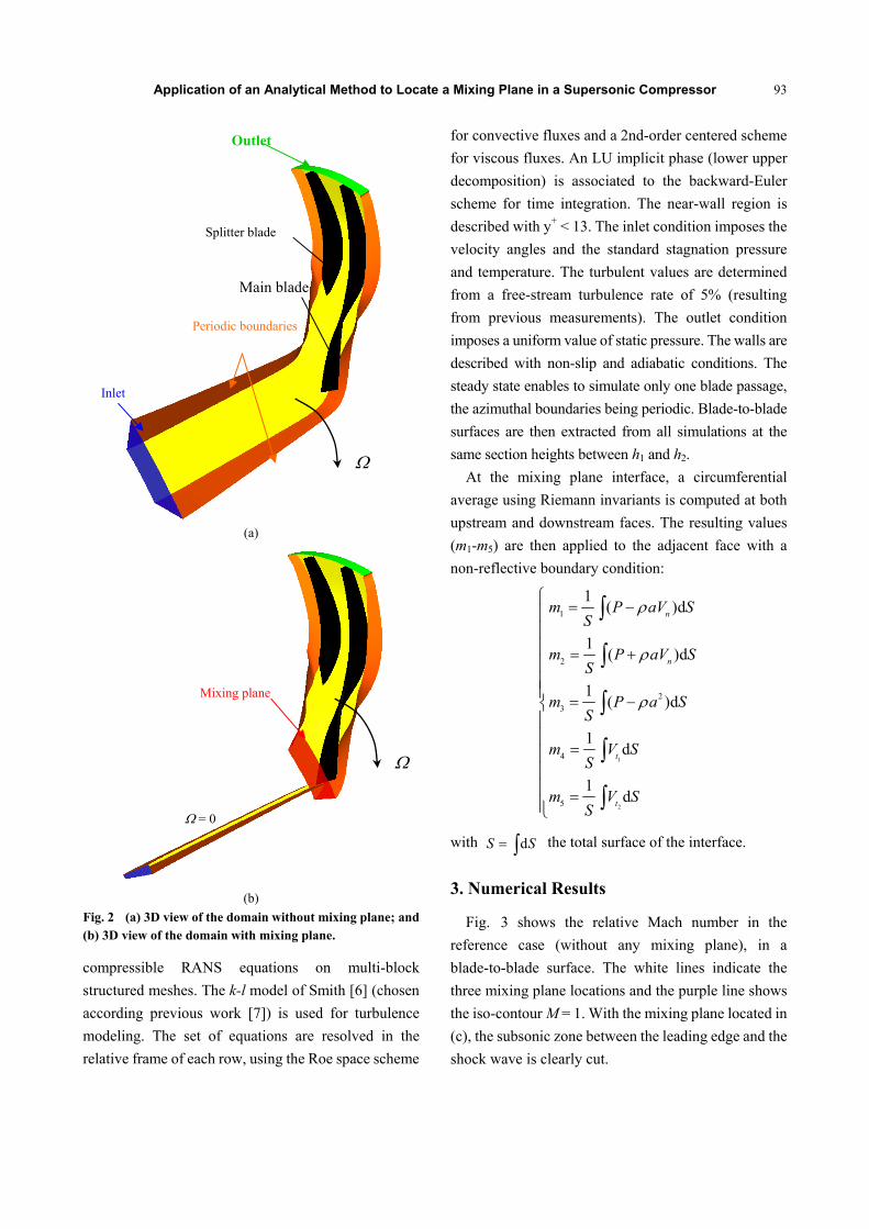
Fig. 2 (a) 3D view of the domain without mixing plane; and (b) 3D view of the domain with mixing plane.

compressible RANS equations on multi-block

structured meshes. The k-l model of Smith [6] (chosen

according previous work [7]) is used for turbulence

modeling. The set of equations are resolved in the

relative frame of each row, using the Roe space scheme

for convective fluxes and a 2nd-order centered scheme

for viscous fluxes. An LU implicit phase (lower upper

decomposition) is associated to the backward-Euler

scheme for time integration. The near-wall region is

described with y+ < 13. The inlet condition imposes the

velocity angles and the standard stagnation pressure

and temperature. The turbulent values are determined

from a free-stream turbulence rate of 5% (resulting

from previous measurements). The outlet condition

imposes a uniform value of static pressure. The walls are

described with non-slip and adiabatic conditions. The

steady state enables to simulate only one blade passage,

the azimuthal boundaries being periodic. Blade-to-blade

surfaces are then extracted from all simulations at the

same section heights between h1 and h2.

At the mixing plane interface, a circumferential

average using Riemann invariants is computed at both

upstream and downstream faces. The resulting values

(m1-m5) are then applied to the adjacent face with a

non-reflective boundary condition:

1

2

1

2

2

3

4

5

1( )d

1( )d

1( )d

1d

1d

n

n

t

t

m P aV SS

m P aV SS

m P a SS

m V SS

m V SS

with dS S the total surface of the interface.

3. Numerical Results

Fig. 3 shows the relative Mach number in the

reference case (without any mixing plane), in a

blade-to-blade surface. The white lines indicate the

three mixing plane locations and the purple line shows

the iso-contour M = 1. With the mixing plane located in

(c), the subsonic zone between the leading edge and the

shock wave is clearly cut.

= 0

Mixing plane

Inlet

Outlet

Periodic boundaries

Main blade

Splitter blade


94

Fig. 3 Relative Mach number without mixing plane.

Fig. 4 shows that in the four configurations, the

detachment distance of the shock remains constant,

which tends to prove that the mixing plane gives a

correct value of the averaged Mach number. Indeed, as

explained in the following, the detachment distance

only depends on the blade geometry and inlet Mach

number. The white lines represent Mach iso-contours

from 0.7 to 1.4.

However, the shape of the subsonic zone is seriously

affected. The more the mixing plane is located

downstream, the less the shock waves can extend

upstream. Thereby, according to the position of the

mixing plane, the total pressure loss is under-estimated.

The change in stagnation pressure can be quantified

with the value of the loss coefficient K calculated as:

1

21t

t

P

PK

with tP , the momentum-averaged relative stagnation

pressure integrated on the whole surface at Section 2

(located at the blade leading edge) and on the whole

surface at Section 1 (located upstream) as:

d

d

t n

St

n

S

P V S

P

V S

Fig. 4 Relative Mach number in the four test cases.

As is expected, the more the mixing plane is located

downstream, the lower the losses are, and consequently,

the more the massflow is over-estimated. Table 1 gives

the difference between overall inlet massflow in cases

Without mixing plane

Case (a)

Case (b)

Case (c)

Section 1 (a) (b) (c) Section 2


95

Table 1 Performance shift to the reference configuration.

Massflow K/Kref

Mixing plane located in (a) +0.04% -1.2%

Mixing plane located in (b) +0.35% -8.3%

Mixing plane located in (c) +0.80% -21.2%

(a), (b), (c) compared to the reference configuration

without mixing plane.

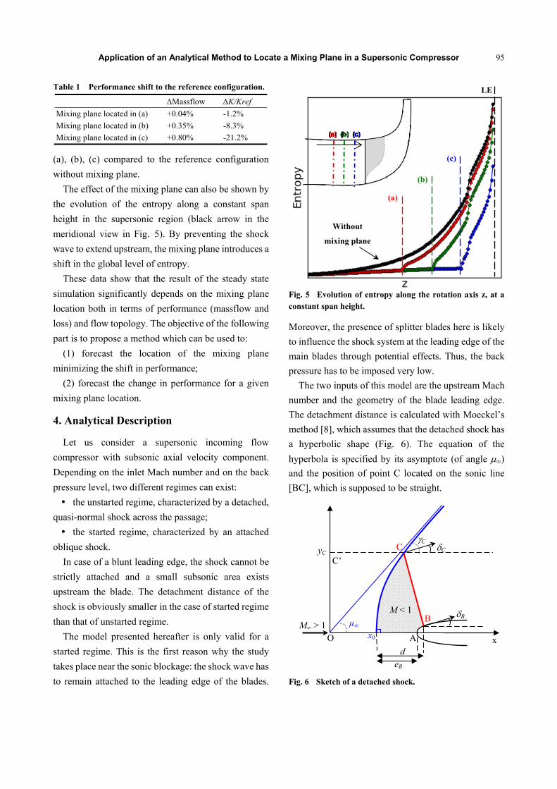
The effect of the mixing plane can also be shown by

the evolution of the entropy along a constant span

height in the supersonic region (black arrow in the

meridional view in Fig. 5). By preventing the shock

wave to extend upstream, the mixing plane introduces a

shift in the global level of entropy.

These data show that the result of the steady state

simulation significantly depends on the mixing plane

location both in terms of performance (massflow and

loss) and flow topology. The objective of the following

part is to propose a method which can be used to:

(1) forecast the location of the mixing plane

minimizing the shift in performance;

(2) forecast the change in performance for a given

mixing plane location.

4. Analytical Description

Let us consider a supersonic incoming flow

compressor with subsonic axial velocity component.

Depending on the inlet Mach number and on the back

pressure level, two different regimes can exist:

the unstarted regime, characterized by a detached,

quasi-normal shock across the passage;

the started regime, characterized by an attached

oblique shock.

In case of a blunt leading edge, the shock cannot be

strictly attached and a small subsonic area exists

upstream the blade. The detachment distance of the

shock is obviously smaller in the case of started regime

than that of unstarted regime.

The model presented hereafter is only valid for a

started regime. This is the first reason why the study

takes place near the sonic blockage: the shock wave has

to remain attached to the leading edge of the blades.

Fig. 5 Evolution of entropy along the rotation axis z, at a constant span height.

Moreover, the presence of splitter blades here is likely

to influence the shock system at the leading edge of the

main blades through potential effects. Thus, the back

pressure has to be imposed very low.

The two inputs of this model are the upstream Mach

number and the geometry of the blade leading edge.

The detachment distance is calculated with Moeckel’s

method [8], which assumes that the detached shock has

a hyperbolic shape (Fig. 6). The equation of the

hyperbola is specified by its asymptote (of angle )

and the position of point C located on the sonic line

[BC], which is supposed to be straight.

Fig. 6 Sketch of a detached shock.

d eB

yC

x

M < 1

O

C C

B

C

µ∞ M∞ > 1B

A x0

C’

(a)

(b)

(c)

Without

mixing plane

LE


96

In order to apply Moeckel’s model, the upstream

flow is supposed to be two-dimensional, uniform and

the profile is approximated by a symmetric shape. The

thermodynamic shock relations for ideal gas are used.

The maximum entropy rise, corresponding to a normal

shock, is located on the streamline passing by the

leading edge. This line and the sonic line are assumed

to be straight. The available equations are:

The equation of the hyperbola:

220

22 )( tgxxy cc (1)

The equation of the tangent at point C:

2tgy

xtg

C

CC

(2)

which, combined with Eq. (1), gives:

2 2

0 2C

C

tg tgx y

tg

(3)

The equation of the distance eB:

2

22

2)(

tg

tgtgy

tgyytg

tgye

CC

CBCC

CB

(4)

In order to calculate the ordinate of point C, yC, the

continuity equation is written between the segment

[OC’] upstream the shock wave and the sonic line

[BC]:

* * * *BCcosC B

C C C C CC

y yV y a a

(5)

which leads to:

CCC

B

C

a

a

a

Vy

y

cos1

1

**

**

**

(6)

Since a shock wave is isenthalpic, we can write: 1

2(1 )2

* *

1(1 )

21

2

M MV

a

(7)

Ct

t

CC P

P

a

a **

**

(8)

It is important to notice that a choice is possible at

that Eq. (8) in the way the stagnation pressure ratio is

calculated. In the present case, a normal shock is

considered at point C:

1

* * 112

* * 2

2 2 11 1 1 1

1 1C C

aM

a M

(9)

It would also be thinkable to consider an oblique

shock to evaluate the thermodynamic state along the

sonic line. This is at the same time a source of

uncertainty in this method and a degree of freedom for

the user (playing on this ratio enables to fit CFD or

measurements but it is rather difficult to give a formula

which works for all types of blades).

The steps of the detachment distance calculation are

thus:

From the value of the inlet Mach number M,

is calculated with:

M

1arcsin

(10)

and the values of the deviation C and shock angle C

are deduced from the shock relations.

Point B which belongs to the profile is identified

from its tangent B which has to be equal to C.

Eqs. (3), (4) and (6) are then used to calculate the

detachment distance d:

ABB xxed (11)

This procedure, initially thought for symmetric

isolated profiles, leads to a geometric representation

of the subsonic zone (in grey in Fig. 6), between

the hyperbola and the sonic line. The part of the

shock wave confining this subsonic region is

responsible for most of the total pressure losses.

Therefore, it is crucial to let it fully extend upstream

the blades. The consequences of a mixing plane

cutting the subsonic pocket are examined in the

following.


97

5. Comparison between Analytical and Numerical Results

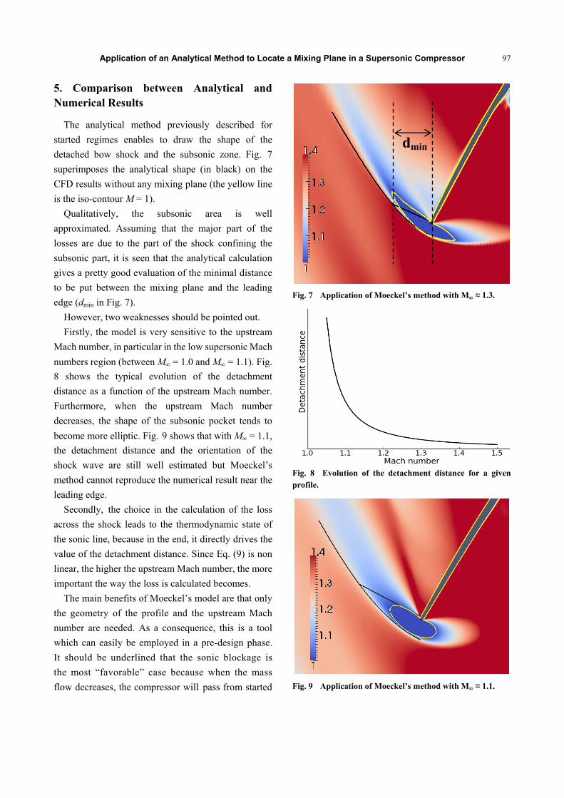
The analytical method previously described for

started regimes enables to draw the shape of the

detached bow shock and the subsonic zone. Fig. 7

superimposes the analytical shape (in black) on the

CFD results without any mixing plane (the yellow line

is the iso-contour M = 1).

Qualitatively, the subsonic area is well

approximated. Assuming that the major part of the

losses are due to the part of the shock confining the

subsonic part, it is seen that the analytical calculation

gives a pretty good evaluation of the minimal distance

to be put between the mixing plane and the leading

edge (dmin in Fig. 7).

However, two weaknesses should be pointed out.

Firstly, the model is very sensitive to the upstream

Mach number, in particular in the low supersonic Mach

numbers region (between M = 1.0 and M = 1.1). Fig.

8 shows the typical evolution of the detachment

distance as a function of the upstream Mach number.

Furthermore, when the upstream Mach number

decreases, the shape of the subsonic pocket tends to

become more elliptic. Fig. 9 shows that with M = 1.1,

the detachment distance and the orientation of the

shock wave are still well estimated but Moeckel’s

method cannot reproduce the numerical result near the

leading edge.

Secondly, the choice in the calculation of the loss

across the shock leads to the thermodynamic state of

the sonic line, because in the end, it directly drives the

value of the detachment distance. Since Eq. (9) is non

linear, the higher the upstream Mach number, the more

important the way the loss is calculated becomes.

The main benefits of Moeckel’s model are that only

the geometry of the profile and the upstream Mach

number are needed. As a consequence, this is a tool

which can easily be employed in a pre-design phase.

It should be underlined that the sonic blockage is

the most “favorable” case because when the mass

flow decreases, the compressor will pass from started

Fig. 7 Application of Moeckel’s method with M ≈ 1.3.

Fig. 8 Evolution of the detachment distance for a given profile.

Fig. 9 Application of Moeckel’s method with M ≈ 1.1.

dmin


98

regime to unstarted regime. Thus, the shock pattern

moves upstream, so that the impact of the mixing plane

can only become stronger.

6. Shock Loss Prediction

Although current blade design relies on numerical

optimization, including transonic bladings [9], many

analytical shock loss models exist, as described in Refs.

[10, 11], for example. Bloch, Copenhaver and O’Brien

also give an interesting approach based on Moeckel’s

method [12], adapted to unstarted regime.

Since the other objective of this paper is to

analytically forecast the change in pressure loss for a

given mixing plane location compared with the

reference case (without any mixing plane), the shock

loss associated to a started regime has to be evaluated.

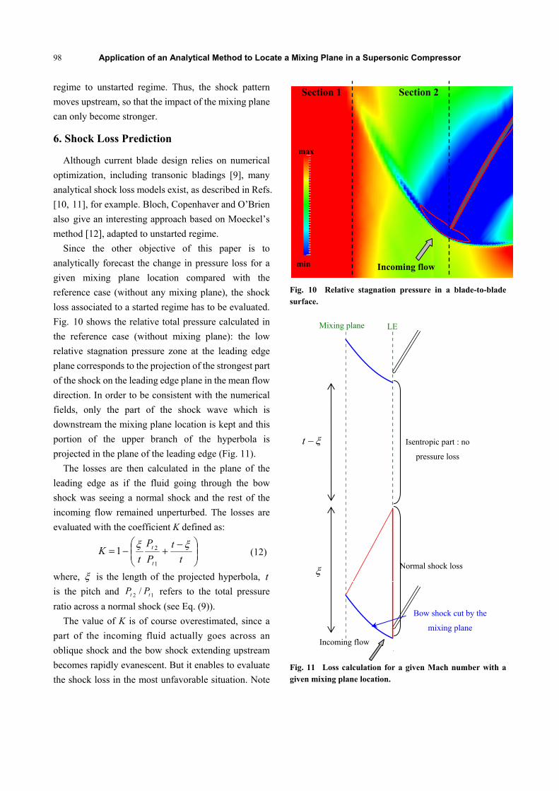
Fig. 10 shows the relative total pressure calculated in

the reference case (without mixing plane): the low

relative stagnation pressure zone at the leading edge

plane corresponds to the projection of the strongest part

of the shock on the leading edge plane in the mean flow

direction. In order to be consistent with the numerical

fields, only the part of the shock wave which is

downstream the mixing plane location is kept and this

portion of the upper branch of the hyperbola is

projected in the plane of the leading edge (Fig. 11).

The losses are then calculated in the plane of the

leading edge as if the fluid going through the bow

shock was seeing a normal shock and the rest of the

incoming flow remained unperturbed. The losses are

evaluated with the coefficient K defined as:

t

t

P

P

tK

t

t

1

21 (12)

where, is the length of the projected hyperbola, t

is the pitch and 12 / tt PP refers to the total pressure

ratio across a normal shock (see Eq. (9)).

The value of K is of course overestimated, since a

part of the incoming fluid actually goes across an

oblique shock and the bow shock extending upstream

becomes rapidly evanescent. But it enables to evaluate

the shock loss in the most unfavorable situation. Note

Fig. 10 Relative stagnation pressure in a blade-to-blade surface.

Fig. 11 Loss calculation for a given Mach number with a given mixing plane location.

Mixing plane

Isentropic part : no

pressure loss

Normal shock loss

Incoming flow

LE

Bow shock cut by the

mixing plane

t

Incoming flow min

max

Section 1 Section 2


99

that in case of no mixing plane, the model is equivalent

to considering a normal shock over the whole pitch.

This choice keeps the present tool simple, but it

would be possible to make a more sophisticated model:

First, by improving the shock wave

approximation. A good example is given by Ottavy

[13], by coupling Levine’s method [14] to predict the

unique incidence seen by the blade profile with

Moeckel’s detachment distance calculation.

By discretizing the shock wave, so that the flow

angle and the pressure loss change from a normal shock

on the blade axis to an oblique shock and integrating

the result on a pitch to the neighboring blade.

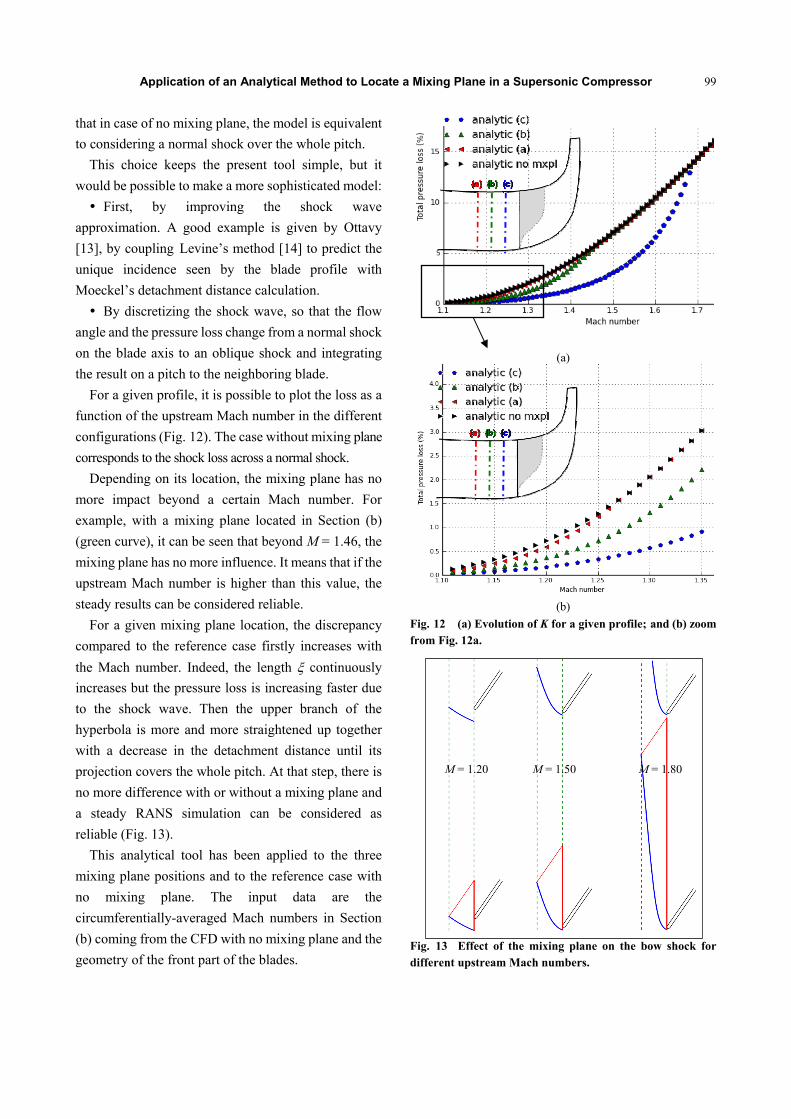
For a given profile, it is possible to plot the loss as a

function of the upstream Mach number in the different

configurations (Fig. 12). The case without mixing plane

corresponds to the shock loss across a normal shock.

Depending on its location, the mixing plane has no

more impact beyond a certain Mach number. For

example, with a mixing plane located in Section (b)

(green curve), it can be seen that beyond M = 1.46, the

mixing plane has no more influence. It means that if the

upstream Mach number is higher than this value, the

steady results can be considered reliable.

For a given mixing plane location, the discrepancy

compared to the reference case firstly increases with

the Mach number. Indeed, the length continuously

increases but the pressure loss is increasing faster due

to the shock wave. Then the upper branch of the

hyperbola is more and more straightened up together

with a decrease in the detachment distance until its

projection covers the whole pitch. At that step, there is

no more difference with or without a mixing plane and

a steady RANS simulation can be considered as

reliable (Fig. 13).

This analytical tool has been applied to the three

mixing plane positions and to the reference case with

no mixing plane. The input data are the

circumferentially-averaged Mach numbers in Section

(b) coming from the CFD with no mixing plane and the

geometry of the front part of the blades.

(a)

(b)

Fig. 12 (a) Evolution of K for a given profile; and (b) zoom from Fig. 12a.

Fig. 13 Effect of the mixing plane on the bow shock for different upstream Mach numbers.

M = 1.20 M = 1.50 M = 1.80


100

Fig. 14 Analytical and numerical loss as function of the upstream Mach number for different mixing plane locations.

Fig. 14 compares the analytical and numerical

values obtained for the losses. Different section heights

between h1 and h2 have been tested, so that both the

profile and the Mach number were changing. The

values of K are plotted as a function of the upstream

Mach number and are calculated as:

1

21t

t

P

PK

where, 2π

02π

0

d

d

t n

t

n

P V r

P

V r

In Fig. 14, the analytical evolution corresponding to

case (a) is the same as the reference one for Mach

numbers greater than 1.30. This means that the major

part of the hyperbola is contained downstream the

mixing plane for the corresponding section heights.

According to this criterion, any mixing plane should be

located upstream Section (a) (Fig. 3) for the present

impeller.

Nevertheless, despite the good qualitative agreement

between analytical and numerical results in Fig. 7, we

can observe quantitative discrepancies in the shock

loss.

First of all, the simulation without mixing plane

describes a different loss evolution around M = 1.20

than those with a mixing plane. This is a well-known

problem with mixing planes in general: the loss is

radially redistributed.

The influence of the location of the mixing plane is

clearly visible in the numerical curves. The slopes are

not so far from the analytical ones. But there is a sort of

offset between the numerical and the analytical results.

It is probable that for the low Mach numbers, the shock

loss is low compared to the viscous loss. To compare

properly the two curves families, it would be necessary

to take from the Navier-Stokes simulations only the

shock loss, as done in Ref. [12] by subtracting the

friction loss from measurements.

The discrepancies are also due to the strong

hypotheses made in the analytical method, which

consists in a two-dimensional approach and due to the

choice made for the loss calculation. Real blade

profiles are also often cambered and not symmetric in

order to produce lift, which is not taken into account in

the present model. And finally, the numerical loss at

the highest Mach numbers (close to the section height

h2) is suddenly increasing, near the shroud boundary

layer. It is likely that friction loss dominates shock loss

in this area.

Thanks to this simple model, the order of magnitude

of the under prediction of the losses due to the

introduction of a mixing plane is easily evaluated. It

has been tested that this approach gives acceptable

results from inlet Mach number larger than 1.1. Once

again, the major drawbacks of this method are that it

gives wrong predictions for lower Mach numbers and

that the shock formulas which are used in it are very

sensitive. This is maybe one of the reasons why Bloch

et al. [12] had to take into account an “effective”

leading edge radius in their model dedicated to predict

the shock loss through the lower branch of Moeckel’s

hyperbola, in supersonic compressor cascades

operating in unstarted regime. Indeed, they increased

the leading edge thickness until the analytical results


101

matched the experimental ones. This reminds us of the

difficulty of implementing a shock loss model that fits

all types of profiles, under various operating

conditions.

7. Conclusion

Steady state numerical simulations performed with a

mixing plane approach show that the results, in terms

of mass flow and losses, significantly depend on the

mixing plane position. The operating point chosen here

corresponds to the sonic blockage of the compressor

but for near-surge points, it would be even more

important.

The fact that this study takes place near the blockage

enables to propose an analytical method in order to

forecast this change in performance. The validity of

this analytical method is checked by comparing its

results with the numerical ones in the entry zone of a

transonic compressor. Analytical and numerical results

show good agreement.

This tool may be useful for transonic compressor

design: first, to have an idea of the minimal distance

that should be put between the mixing plane and the

leading edge of the blades, and then to know how

representatively the steady simulations can be

expected.

Acknowledgements

We would like to thank Turbomeca which supported

this study, together with ONERA which collaborated

on the numerical simulation. This work was granted

access to the HPC resources of CINES under the

allocation 2013-2a6356.

References

[1] Lichtfuss, J. J., and Starken, H. 1974. “Supersonic Cascade Flow.” Progress in Aerospace Sciences 15: 37-149.

[2] Kantrowitz, A. 1946. The Supersonic Axial-Flow Compressor. NACA technical report.

[3] Chauvin, J. 1970. Supersonic Turbo-Jet Propulsion Systems and Components. AGARD report No. 120.

[4] Trébinjac, I., Ottavy, X., Rochuon, N., and Bulot, N. 2009. “On the Validity of Steady Calculations with Shock-Blade Row Interaction in Compressors.” In Proceedings of the 9th International Symposium on Experimental and Computational Aerothermodynamics of Internal Flows, ISAIF9-062.

[5] Cambier, L., and Gazaix, M. 2002. “elsA: An Efficient Object-Oriented Solution to CFD Complexity.” Presented at 2002 the 40th AIAA Aerospace Science Meeting and Exhibit, Reno, USA.

[6] Smith, B. R. 1995. “Prediction of Hypersonic Shock Wave Turbulent Boundary Layer Interactions with k-l Two-Equations Turbulence Model.” Presented at 1995 the 33rd AIAA Aerospace Sciences Meeting and Exhibition, Reno, USA.

[7] Rochuon, N. 2007. “Analysis of the Three-Dimensional Unsteady Flow in a High Pressure Ratio Centrifugal Compressor.” Ph.D. thesis, École centrale de Lyon.

[8] Moeckel, W. E. 1942. Approximate Method for Predicting Form and Location of Detached Shock Waves. NACA technical report.

[9] Burguburu, S., Toussaint, C., Bonhomme, C., and Leroy, G. 2004. “Numerical Optimization of Turbomachinery Bladings.” Journal of Turbomachinery 126 (1): 91-100.

[10] König, W. M., Hennecke, D. K., and Fottner, L. 1996. “Improved Blade Profile Loss and Deviation Angle Models for Advanced Transonic Compressor Bladings: Part II—A Model for Supersonic Flow.” Journal of Turbomachinery 118 (1): 81-7.

[11] Schobeiri, M. T. 1997. “Advanced Compressor Loss Correlations, Part I: Theroretical Aspects.” International Journal of Rotating Marchinery 3 (3): 163-77.

[12] Bloch, G. S., Copenhaver, W. W., and O’Brien, W. F. 1999. “A Shock Loss Model for Supersonic Compressor Cascades.” Journal of Turbomachinery 121 (1): 28-35.

[13] Ottavy, X. 1999. “Laser Anemometry Measurements in an Axial Transonic Compressor. Analysis of the Unsteady Periodic Structures.” Ph.D. thesis, École centrale de Lyon.

[14] Levine, P. 1956. The Two-Dimensional Inflow Conditions for a Supersonic Compressor with Curved Blades. WADC technical report 55-387.

Application of an Analytical Method to Locate a Mixing ... · PDF fileApplication of an...

Documents

Transcript of Application of an Analytical Method to Locate a Mixing ... · PDF fileApplication of an...