APPLICATION OF AGROMETEOROLOGY TO AQUACULTURE AND · PDF file ·...

APPLICATION OF AGROMETEOROLOGY TO AQUACULTURE AND FISHERIES

13.1 INTRODUCTION

The products of feisheries have been an important component of the world food supply for centuries. The number of global capture fisheries has increased in response to the demands of rising human popula-tion. The Food and Agriculture Organization (FAO) of the United Nations began keeping statistics on world fisheries production in the 1950s; since then, the annual catch from capture fisheries has increased from about 25 million tonnes to approximately 95 million tonnes. Most authorities feel that capture fisheries around the world are exploited to or possi-bly beyond their sustainable limit. For its part, aquaculture has been growing in importance: in 2004 the supply from aquaculture reached 59 million tonnes, or 38.1 per cent of world fisheries produc-tion. The world’s population will continue to grow and demand for products from fisheries will also rise accordingly. Aquaculture must step in to meet this increasing demand, for the catch by capture fisheries apparently cannot be increased.

Meteorology plays an important role in fisheries because solar radiation and air temperature influence water temperature, which in turn affects the natural productivity of inland and marine waters and the growth of fisheries species (Kapetsky, 2000). Weather conditions also have a tremendous effect on the abil-ity of fishermen to capture fish and other aquatic organisms, and on the safety of fishermen. Nonetheless, fishing, like hunting and gathering, primarily involves the exploitation of living resources from natural populations; the management of these resources is limited largely to regulations on capture.

Aquaculture will soon surpass fisheries as the major source of aquatic protein, just as agriculture surpassed hunting and gathering as a source of meat, grain and other foods. Agrometeorology has become an important tool in agriculture and it can be equally useful in aquaculture. Meteorological data are already used in aquaculture (Szumiec, 1983; Boyd and Tucker, 1998; Kapetsky, 2000). Nevertheless, there have been few attempts to organize the effort so that the acquisition and application of meteorological data may also serve as a tool for practical aquaculturists and become an important part of the training of aquacultural scientists. The purpose of this report is to discuss the application of meteorological data in fisheries

and especially in aquaculture. It is hoped that this discussion will encourage the application of existing agrometeorological information to aquatic animal production and stimulate research on the topic.

13.2 CAPTUREFISHERIES

Most of the commercial catch of fisheries products is of marine origin; in 2004, 87.2 million tonnes were taken from the oceans, compared with 8.7 million tonnes from inland waters. The Asian region accounted for nearly half of the production. China was the top fishing country, and four other Asian nations were in the top ten. During the past 10 years, the world production of capture fisheries has fluctu-ated between 88 million tonnes and 96 million tonnes, with no upward or downward trend. Many species have been overfished and pollution of the oceans and coastal waters has negatively affected productivity. The production of wild fish popula-tions is dependent upon optimum temperature and other favourable weather conditions. Meteorological data can be used in attempts to explain observed changes in fisheries production. Forecasts of tempo-rary or long-term changes in climate can also be used to predict changes in fisheries populations that could influence the future catch.

Most fishing methods require operation of boats in large bodies of water and are inherently dangerous activities because of storms. Short-term weather forecasts can be extremely useful for planning fish-ing activities. Moreover, information on the intensity and tracks of storms is critical to the safety of fishermen. Historically, many fishermen have perished because of inadequate information about storms or because of a failure to heed warnings.

13.3 AQUACULTURE

Total world aquaculture production was 59.4 million tonnes in 2004. Of this, 32.2 million tonnes originated from freshwater aquaculture and 27.2 million tonnes from marine aquaculture. The top five countries in the world in terms of aquacul-ture production are in Asia, as are 11 of the top £ 15 producers, and China accounts for over one half

CHAPTER 13

GUIDE TO AGRICULTURAL METEOROLOGICAL PRACTICES 13–2

of the world aquaculture production. Although aquaculture is vital to the domestic food supply of many nations, aqua culture products also are impor-tant international commodities. For example, the United States imports nearly 80 per cent of its seafood, and many of these products are from aqua-culture. Aquaculture production systems vary greatly both among and within species. An overview of the common production systems will be useful to read-ers who may not be familiar with aquaculture.

13.3.1 Pondculture

Aquatic animals are stocked in ponds, and fertilizer and feed are used to promote rapid growth. Undesirable species can be excluded and water quality maintained within a desirable range. Production per unit area greatly exceeds that of natural waters and culture animals can be harvested easily. Three basic types of ponds are used in aqua-culture: watershed ponds, embankment ponds and excavated ponds. The water budget for ponds may be expressed by the hydrologic equation:

Inflow – outflow = ∆H (13.1)

The hydrologic equation for ponds may be expanded as follows:

(P + R + Sin + A) – (E + So + O + C + Q) = ∆H (13.2)

where P = precipitation; R = runoff; Sin = seepage in; A = intentional additions from wells, streams, lakes or other sources; E = evaporation; So = seepage out; O = overflow; C = consumptive use for domestic use, irrigation, livestock watering or other purposes; Q = intentional discharge for water exchange or harvesting; and ∆H = change in storage. Depending upon its design, construction, location and use, one or more of the terms listed above may not apply to a specific pond.

Watershed ponds are made by building a dam across a watercourse to impound surface runoff. They vary greatly in area, but most are greater than 0.5 ha and less than 10 ha in area. These ponds also have been called terrace ponds, and it is common to construct a series of them on a watershed so that the overflow from one pond will be captured by another at a lower elevation. Watershed ponds fill and often overflow during the rainy season, but the water level may decline drastically during dry weather. The minimum ratio of watershed area to pond volume necessary to maintain watershed ponds varies from about 0.3 ha/1 000 m3 in moun-tainous, humid areas to over 40 ha/1 000 m3 in

arid, plains regions (United States Soil Conservation Service, 1979). The fluctuation in water level in watershed ponds ranges from a few centimetres to more than a metre, with the greatest fluctuations occurring in arid climates, during droughts, and in ponds that seep excessively (Yoo and Boyd, 1994). Some ponds are never drained, while others may be drained annually for harvest. Sometimes, ponds may have multiple uses, and water may be with-drawn for domestic use, livestock watering or irrigation.

Excavated ponds are made by digging a basin in which to store water. Ponds may be filled by rain-fall, runoff and infiltration of ground water. Such ponds cannot be drained, but sometimes water may be removed with a pump. Small, excavated ponds of a few hundred square metres in area are widely used for aquaculture in rural areas of India, Bangladesh and some other Asian countries. These ponds also may serve as sources of water for home and farm uses. Where direct rainfall is the major source of water for excavated ponds, ponds may dry up or become very shallow during the dry season.

Watershed and excavated ponds rarely receive inflow from wells, streams or other external bodies of water. Fisheries production in such ponds often is referred to as “rainfed” aquaculture. Rainfall, overland flow, evaporation and seepage are critical factors regulating the amount of water available for rainfed aquaculture. Small, rainfed ponds are the most common aquaculture systems used by poor, rural people in tropical nations.

Embankment ponds are formed by building an embankment around the area for water storage. Surface areas of these ponds often are 0.2 to 2 ha and seldom over 10 ha. Watersheds consist of the above-water, inside slopes of embankments, and little runoff enters ponds. Embankment ponds in inland areas are supplied with water from wells, streams or reservoirs. In coastal areas, embank-ment ponds are filled with brackish water from estuaries or seawater. Drain structures consist of pipes with valves or gates with dam boards. Embankment ponds are popular for commercial aquaculture because water levels can be controlled and ponds drained easily to facilitate harvest. These ponds usually are dedicated to aquaculture use and are not sources of water for other activities.

13.3.2 Flow-throughsystems

Flow-through systems for aquaculture include race-ways, tanks and other culture units through which

CHAPTER 13. APPLICATION OF AGROMETEOROLOGY TO AQUACULTURE AND FISHERIES 13–3

water flows continuously. The culture species is stocked at densities much greater than those used in ponds (Table 13.1). Water flow rates normally are two or three times the volume of the culture units per hour. Water sources are springs, streams and other bodies of surface water. Incoming water is the main source of dissolved oxygen for fish and wastes are flushed from culture units by the flowing water. A constant supply of water is essential for flow-through systems. These systems are especially popular for the culture of trout in freshwater.

13.3.3 Open-waterculturemethods

Aquatic organisms also are cultured in open waters of oceans, estuaries, lakes and streams by confining them at high density (Table 13.1) in enclosures or by placing sessile organisms on bottom plots or attaching them to a structural framework. Cages and net pens are constructed of netting secured to a supporting framework. Cages vary in size from 1 m3 to more than 2 000 m3, and they float on or near the water surface. Fish in cages are supplied with manufactured feed daily. Pens are made by install-ing vertical poles and attaching netting to form an enclosure in which to culture fish. Pens are larger than cages and stocked at lower densities than cages (FAO, 1984). The fish in pens usually are fed, and they have free access to natural food organisms in the water and sediment of the enclosed area.

Bivalve shellfish such as oysters, clams, mussels and scallops can be laid on bottom plots in coastal waters for grow-out. It is more common, however, to place young shellfish, called spat, on stakes, rocks and racks, or to attach them to ropes hanging from long lines, rafts or other structures for grow-out by off-bottom culture methods. These structures are placed in coastal waters in areas often used for navigation, fishing or other purposes. Seaweed is usually attached to ropes or netting for grow-out in coastal waters.

13.3.4 Water-reusesystems

There are two basic types of water recirculation systems. One type is built outdoors and consists of culture units from which water passes through a sedimentation basin and then into a larger, earthen pond for treatment by natural biological processes before being returned to the culture units for reuse. Mechanical aeration sometimes is applied in the treatment pond to enhance dissolved oxygen concentration and promote microbial activity. The other type of water-reuse system usually is placed in a greenhouse or other structure: water from culture units passes through mechanical and biological filters and is aerated before being reused in culture units. Effluents may overflow from outdoor systems during rainy weather, and water must occasionally be discharged from indoor systems when new water is applied to lower salinity or filters are cleaned.

Culture method Standing biomass

Ponds (fish and shrimp)

Extensive 0.025 to 0.05 kg m–3

Semi-intensive 0.05 to 0.5 kg m–3

Intensive 0.5 to 5 kg m–3

Flow-through systems

Trout 160 to 240 kg m–3

Channel catfish 75 to 150 kg m–3

Carp 200 to 300 kg m–3

Cages

Trout 20 to 40 kg m–3

Tilapia 150 to 250 kg m–3

Channel catfish 100 to 200 kg m–3

Water-recirculating systems (finfish) 100 to 200 kg m–3

Shellfish plots 0.5 to 150 kg m–2

Table 13.1. Typical standing biomass ranges for different kinds of aquaculture


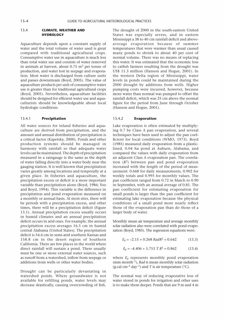
13.4 CLIMATE,WEATHERANDHYDROLOGY

Aquaculture depends upon a constant supply of water and the total volume of water used is great compared with traditional agricultural crops. Consumptive water use in aquaculture is much less than total water use and consists of water removed in animals at harvest, about 0.75 m3 per tonne of production, and water lost in seepage and evapora-tion. Most water is discharged from culture units and passes downstream (Boyd, 2005). The value of aquaculture products per unit of consumptive water use is greater than for traditional agricultural crops (Boyd, 2005). Nevertheless, aquaculture facilities should be designed for efficient water use and aqua-culturists should be knowledgeable about local hydrologic conditions.

13.4.1 Precipitation

All water sources for inland fisheries and aqua-culture are derived from precipitation, and the amount and annual distribution of precipitation is a critical factor (Kapetsky, 2000). Ponds and other production systems should be managed in harmony with rainfall so that adequate water levels can be maintained. The depth of precipitation measured in a raingauge is the same as the depth of water falling directly into a water body near the gauging station. It is well known that precipitation varies greatly among locations and temporally at a given place. In fisheries and aqua culture, the precipitation excess or deficit is a more important variable than precipitation alone (Boyd, 1986; Yoo and Boyd, 1994). This variable is the difference in precipitation and pond evaporation measured on a monthly or annual basis. At most sites, there will be periods with a precipitation excess, and other times, there will be a precipitation deficit (Figure 13.1). Annual precipitation excess usually occurs in humid climates and an annual precipitation deficit occurs in arid ones. For example, the annual precipitation excess averages 16.5 cm in humid central Alabama (United States). The precipitation deficit is 54.6 cm in semi-arid southern Kansas and 158.8 cm in the desert region of Southern California. There are few places in the world where direct rainfall will sustain a pond. There usually must be one or more external water sources, such as runoff from a watershed, inflow from seepage or additions from wells or other water bodies.

Drought can be particularly devastating in watershed ponds. Where groundwater is not available for refilling ponds, water levels may decrease drastically, causing overcrowding of fish.

The drought of 2000 in the south-eastern United States was especially severe, and in eastern Mississippi a 38 to 40 cm rainfall deficit and above-average evaporation because of summer temperatures that were warmer than usual caused many ponds to shrink to about 40 per cent of normal volume. There was no means of replacing this water. It was estimated that the economic loss to catfish farmers resulting from the drought was US$ 11.3 million (Hanson and Hogue, 2001). In the western Delta region of Mississippi, water levels in ponds could be maintained during the 2000 drought by additions from wells. Higher pumping costs were incurred, however, because more water than normal was pumped to offset the rainfall deficit, which was 25 cm above the normal figure for the period from June through October (Hanson and Hogue, 2001).

13.4.2 Evaporation

Lake evaporation is often estimated by multiply-ing 0.7 by Class A pan evaporation, and several techniques have been used to adjust the pan coef-ficient for local conditions (WMO, 1973). Boyd (1985) measured daily evaporation from a plastic-lined, 0.04 ha pond at Auburn, Alabama, and compared the values with daily evaporation from an adjacent Class A evaporation pan. The correla-tion (R2) between pan and pond evaporation increased with the length of the period of meas-urement: 0.668 for daily measurements, 0.902 for weekly totals and 0.995 for monthly values. The pan coefficient ranged from 0.72 in March to 0.90 in September, with an annual average of 0.81. The pan coefficient for estimating evaporation for small ponds is larger than the pan coefficient for estimating lake evaporation because the physical conditions of a small pond more nearly reflect those of the evaporation pan than do those of a larger body of water.

Monthly mean air temperature and average monthly solar radiation also were correlated with pond evapo-ration (Boyd, 1985). The regression equations were:

Ep = –2.15 + 0.268 Rad R2 = 0.642 (13.3)

Ep = –4.406 + 5.753 T R2 = 0.862 (13.4)

where Ep represents monthly pond evaporation (mm month–1), Rad is mean monthly solar radiation (g·cal cm–2 day–1) and T is air temperature (°C).

The normal way of reducing evaporative loss of water stored in ponds for irrigation and other uses is to make them deeper. Ponds that are 9 m and 4 m


deep and are exposed to the same conditions will have the same amount of evaporation from their surfaces. Nevertheless, the evaporation loss per cubic metre of water storage will be more from the shallower pond by a factor of 9/4. In aquaculture, it usually is not possible to use this approach to reduce water loss by evaporation because deep ponds strat-ify thermally, making management more difficult.

Evapotranspiration usually is not a major factor in aquaculture ponds because vascular aquatic plants are discouraged by deepening pond edges, by turbidity resulting from plankton and by application of aquatic weed control techniques (Boyd and Tucker, 1998). Nevertheless, in hydrologic a s ses sment o f aquacul ture pro jec t s , evapotranspiration on watersheds is an issue. Yoo and Boyd (1994) recommend the Thornthwaite method to estimate evapotranspiration for aquaculture and fisheries purposes because it requires only information on mean monthly air temperature. Other methods of measuring

evapotranspiration require equipment or data seldom available to aquaculturists.

13.4.3 Overlandflowandrunoff

The amount of overland flow entering ponds depends upon the watershed area, amount of precipitation, infiltration, evapotranspiration and the runoff-producing characteristics of watersheds. Individual watersheds vary greatly with respect to the percentage of precipitation that is transformed to overland flow. Steep, impervious watersheds may yield 75 per cent overland flow, while flat water-sheds with sandy soils may yield less than 10 per cent overland flow. Estimates of overland flow can be made using the curve number method (United States Soil Conservation Service, 1972). In this method, the depth of overland flow is estimated from the depth of rainfall produced by a given storm, antecedent soil moisture conditions, hydro-logic soil group, land use and hydrologic condition on a watershed.

Jan Feb Mar Apr May Jun Jul Aug Sep Oct Nov DecJan Feb Mar Apr May Jun Jul Aug Sep Oct Nov Dec

Jan Feb Mar Apr May Jun Jul Aug Sep Oct Nov Dec Jan Feb Mar Apr May Jun Jul Aug Sep Oct Nov Dec

Dallas,Texas

Preciptation andpond evaporation, mm

Preciptation andpond evaporation, mm

Fresno,California

Auburn,Alabama

Bangkok,Thailand

Figure 13.1. Pond evaporation (solid line) and precipitation (dotted line) at four sites. Dark shading indi-cates an evaporation excess, while light stippling indicates a precipitation excess. (Data from Wallis, 1977;

Farnsworth and Thompson, 1982; Boyd, 1985; and Meteorological Department of Thailand, 1981)


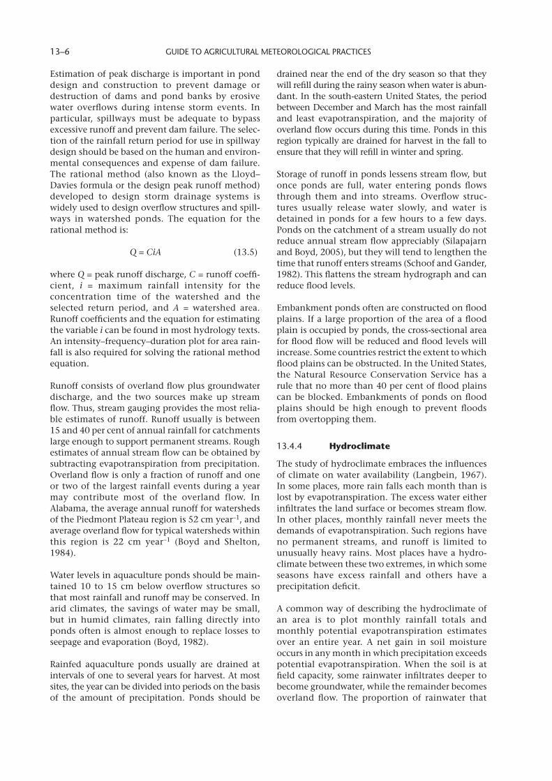
Estimation of peak discharge is important in pond design and construction to prevent damage or destruction of dams and pond banks by erosive water overflows during intense storm events. In particular, spillways must be adequate to bypass excessive runoff and prevent dam failure. The selec-tion of the rainfall return period for use in spillway design should be based on the human and environ-mental consequences and expense of dam failure. The rational method (also known as the Lloyd–Davies formula or the design peak runoff method) developed to design storm drainage systems is widely used to design overflow structures and spill-ways in watershed ponds. The equation for the rational method is:

Q = CiA (13.5)

where Q = peak runoff discharge, C = runoff coeffi-cient, i = maximum rainfall intensity for the concentration time of the watershed and the selected return period, and A = watershed area. Runoff coefficients and the equation for estimating the variable i can be found in most hydrology texts. An intensity–frequency–duration plot for area rain-fall is also required for solving the rational method equation.

Runoff consists of overland flow plus groundwater discharge, and the two sources make up stream flow. Thus, stream gauging provides the most relia-ble estimates of runoff. Runoff usually is between 15 and 40 per cent of annual rainfall for catchments large enough to support permanent streams. Rough estimates of annual stream flow can be obtained by subtracting evapotranspiration from precipitation. Overland flow is only a fraction of runoff and one or two of the largest rainfall events during a year may contribute most of the overland flow. In Alabama, the average annual runoff for watersheds of the Piedmont Plateau region is 52 cm year–1, and average overland flow for typical watersheds within this region is 22 cm year–1 (Boyd and Shelton, 1984).

Water levels in aquaculture ponds should be main-tained 10 to 15 cm below overflow structures so that most rainfall and runoff may be conserved. In arid climates, the savings of water may be small, but in humid climates, rain falling directly into ponds often is almost enough to replace losses to seepage and evaporation (Boyd, 1982).

Rainfed aquaculture ponds usually are drained at intervals of one to several years for harvest. At most sites, the year can be divided into periods on the basis of the amount of precipitation. Ponds should be

drained near the end of the dry season so that they will refill during the rainy season when water is abun-dant. In the south-eastern United States, the period between December and March has the most rainfall and least evapotranspiration, and the majority of overland flow occurs during this time. Ponds in this region typically are drained for harvest in the fall to ensure that they will refill in winter and spring.

Storage of runoff in ponds lessens stream flow, but once ponds are full, water entering ponds flows through them and into streams. Overflow struc-tures usually release water slowly, and water is detained in ponds for a few hours to a few days. Ponds on the catchment of a stream usually do not reduce annual stream flow appreciably (Silapajarn and Boyd, 2005), but they will tend to lengthen the time that runoff enters streams (Schoof and Gander, 1982). This flattens the stream hydrograph and can reduce flood levels.

Embankment ponds often are constructed on flood plains. If a large proportion of the area of a flood plain is occupied by ponds, the cross-sectional area for flood flow will be reduced and flood levels will increase. Some countries restrict the extent to which flood plains can be obstructed. In the United States, the Natural Resource Conservation Service has a rule that no more than 40 per cent of flood plains can be blocked. Embankments of ponds on flood plains should be high enough to prevent floods from overtopping them.

13.4.4 Hydroclimate

The study of hydroclimate embraces the influences of climate on water availability (Langbein, 1967). In some places, more rain falls each month than is lost by evapotranspiration. The excess water either infiltrates the land surface or becomes stream flow. In other places, monthly rainfall never meets the demands of evapotranspiration. Such regions have no permanent streams, and runoff is limited to unusually heavy rains. Most places have a hydro-climate between these two extremes, in which some seasons have excess rainfall and others have a precipitation deficit.

A common way of describing the hydroclimate of an area is to plot monthly rainfall totals and monthly potential evapotranspiration estimates over an entire year. A net gain in soil moisture occurs in any month in which precipitation exceeds potential evapotranspiration. When the soil is at field capacity, some rainwater infiltrates deeper to become groundwater, while the remainder becomes overland flow. The proportion of rainwater that


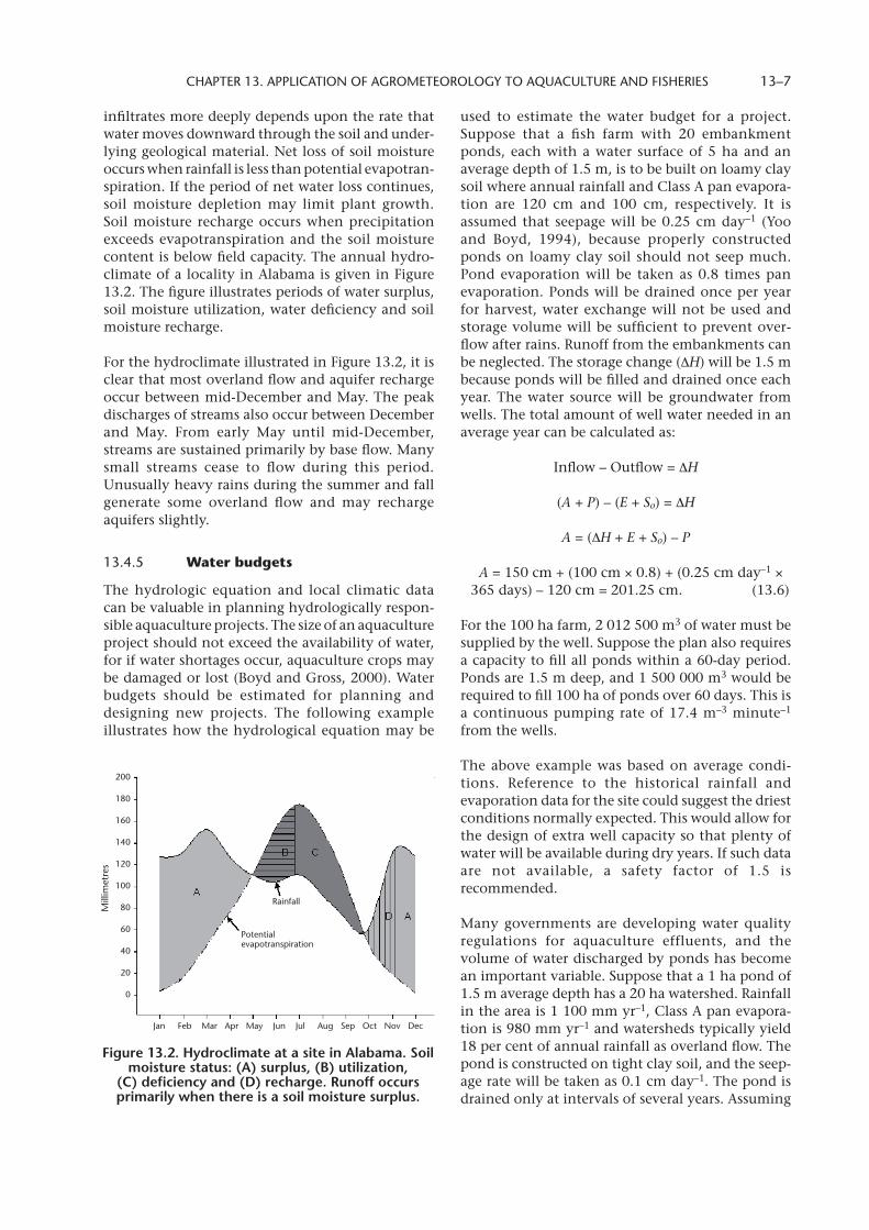
infiltrates more deeply depends upon the rate that water moves downward through the soil and under-lying geological material. Net loss of soil moisture occurs when rainfall is less than potential evapotran-spiration. If the period of net water loss continues, soil moisture depletion may limit plant growth. Soil moisture recharge occurs when precipitation exceeds evapotranspiration and the soil moisture content is below field capacity. The annual hydro-climate of a locality in Alabama is given in Figure 13.2. The figure illustrates periods of water surplus, soil moisture utilization, water deficiency and soil moisture recharge.

For the hydroclimate illustrated in Figure 13.2, it is clear that most overland flow and aquifer recharge occur between mid-December and May. The peak discharges of streams also occur between December and May. From early May until mid-December, streams are sustained primarily by base flow. Many small streams cease to flow during this period. Unusually heavy rains during the summer and fall generate some overland flow and may recharge aquifers slightly.

13.4.5 Waterbudgets

The hydrologic equation and local climatic data can be valuable in planning hydrologically respon-sible aquaculture projects. The size of an aquaculture project should not exceed the availability of water, for if water shortages occur, aquaculture crops may be damaged or lost (Boyd and Gross, 2000). Water budgets should be estimated for planning and designing new projects. The following example illustrates how the hydrological equation may be

used to estimate the water budget for a project. Suppose that a fish farm with 20 embankment ponds, each with a water surface of 5 ha and an average depth of 1.5 m, is to be built on loamy clay soil where annual rainfall and Class A pan evapora-tion are 120 cm and 100 cm, respectively. It is assumed that seepage will be 0.25 cm day–1 (Yoo and Boyd, 1994), because properly constructed ponds on loamy clay soil should not seep much. Pond evaporation will be taken as 0.8 times pan evaporation. Ponds will be drained once per year for harvest, water exchange will not be used and storage volume will be sufficient to prevent over-flow after rains. Runoff from the embankments can be neglected. The storage change (∆H) will be 1.5 m because ponds will be filled and drained once each year. The water source will be groundwater from wells. The total amount of well water needed in an average year can be calculated as:

Inflow – Outflow = ∆H

(A + P) – (E + So) = ∆H

A = (∆H + E + So) – P

A = 150 cm + (100 cm × 0.8) + (0.25 cm day–1 × 365 days) – 120 cm = 201.25 cm. (13.6)

For the 100 ha farm, 2 012 500 m3 of water must be supplied by the well. Suppose the plan also requires a capacity to fill all ponds within a 60-day period. Ponds are 1.5 m deep, and 1 500 000 m3 would be required to fill 100 ha of ponds over 60 days. This is a continuous pumping rate of 17.4 m–3 minute–1 from the wells.

The above example was based on average condi-tions. Reference to the historical rainfall and evaporation data for the site could suggest the driest conditions normally expected. This would allow for the design of extra well capacity so that plenty of water will be available during dry years. If such data are not available, a safety factor of 1.5 is recommended.

Many governments are developing water quality regulations for aquaculture effluents, and the volume of water discharged by ponds has become an important variable. Suppose that a 1 ha pond of 1.5 m average depth has a 20 ha watershed. Rainfall in the area is 1 100 mm yr–1, Class A pan evapora-tion is 980 mm yr–1 and watersheds typically yield 18 per cent of annual rainfall as overland flow. The pond is constructed on tight clay soil, and the seep-age rate will be taken as 0.1 cm day–1. The pond is drained only at intervals of several years. Assuming

Jan Feb Mar Apr May Jun Jul Aug Sep Oct Nov Dec

Mill

imet

res

Potentialevapotranspiration

Rainfall

200

180

160

140

120

100

80

60

40

20

0

Figure 13.2. Hydroclimate at a site in Alabama. Soil moisture status: (A) surplus, (B) utilization,

(C) deficiency and (D) recharge. Runoff occurs primarily when there is a soil moisture surplus.


that the pond typically is full but not overflowing on 1 January of each year, that is, ∆H = 0 cm, the overflow for a year will be estimated. The appropri-ate form of the hydrologic equation and its solution are:

(P + R) – (E + So + O) = ∆H

O = ∆H – (P + R) + (E + So)

O = 0.0 cm – (1.1 m × 1 ha) – (1.1 m × 0.18 × 20 ha) + (0.98 m × 0.8) + (0.001 m day–1 ×

365 days) × 104 = 39 100 m3 year–1

O = –39 110 m3 year–1 (13.7)

The overflow has a negative sign because it repre-sents water lost from the pond. This volume of overflow is more than twice the pond volume.

The overflow estimated in the example above is for an entire year. The spillway design, however, should be based on the most runoff expected following the largest single daily rainfall event for a selected return period, namely, the 25-year, 50-year or 100-year rainfall event (Yoo and Boyd, 1994).

13.5 CLIMATE,WEATHERANDWATERQUALITY

Solar radiation is necessary for aquatic plant growth and is a major factor regulating water temperature. Wind mixing has a strong influence on the thermal and chemical dynamics of water bodies. Finally, extreme weather events such as floods, droughts, hurricanes and unseasonable temperatures can adversely influence water quality and have negative impacts on fisheries and aquaculture.

13.5.1 Solarradiation

Phytoplankton are the base of the food chain that culminates in fisheries production in natural systems. Planktonic algae require solar radiation, water and inorganic nutrients to conduct photosynthesis, a process by which they use chlorophyll and other pigments to capture photons of light and transfer the energy to organic matter. The photosynthesis reaction is provided below in its simplest form:

6CO2 + 6H2O C6H12O6 + 6H2O

Inorganic nutrients

(13.8)

Organisms use oxygen in respiration in order to oxidize organic nutrients and release biologically useful energy. Ecologically, respiration is basically the opposite of photosynthesis. During daylight, photosynthesis usually produces oxygen faster than oxygen is consumed in respiration, and dissolved oxygen concentration increases from morning to afternoon (Figure 13.3). Photosynthesis stops at night, but respiration continues to cause dissolved oxygen concentration to decline at night (Figure 13.3). Differences in dissolved oxygen concentration between day and night become more extreme as phytoplankton abundance increases (Figure 13.3). Aquaculture ponds typically have dense plankton blooms and wide daily fluctuations in dissolved oxygen concentration.

Organic matter from photosynthesis is the source of organic compounds used by phytoplankton and other plants to elaborate their biomass. The oxygen released by the process is a major source of dissolved oxygen needed in respiration by aquatic animals, bacteria and aquatic plants living in water bodies. In aquaculture, fertilizers may be applied to ponds to increase phytoplankton productivity and permit greater aquatic animal production, but manufac-tured feeds may be offered to culture animals to increase production beyond that achievable from natural food.

Although it is well known that short-term varia-tions in the photosynthesis rate result from the effect of cloud cover on the amount of incoming radiation, it has not been demonstrated that the growth rate in aquatic animals is affected by this variation. For most fisheries species, there is a time lag between primary production and its use in fish

Dis

solv

ed

oxy

ge

n (

mg

/L)

Time of day

Heavy plankton bloomModerate plankton bloomLight plankton bloom

6 a.m. Noon 6 p.m. Midnight 6 a.m.

Figure 13.3. Effect of time of day and phyto-plankton density on concentrations of dissolved

oxygen in surface water


production (McConnell, 1963), and short-term fluctuations in solar radiation are not reflected in fluctuations in the growth of fish, shrimp and other fisheries species. Fisheries production integrates short-term fluctuations in solar radiation and photosynthesis, but differences may be obvious on an annual basis. Doyle and Boyd (1984) studied sunfish production in three ponds at Auburn, Alabama, each stocked, fertilized and managed the same way for eight consecutive years. Fish produc-tion averaged 362 kg ha–1 and varied from 270 to 418 kg ha–1 over the period, with a coefficient of variation of 27 per cent. Several factors, including dates of stocking and harvest, water temperature, fish size at stocking and amounts of aquatic weeds in ponds, varied among years and no doubt influ-enced production. Average daily solar radiation data for the period April through September at a nearby site, however, exhibited a positive correla-tion (R2 = 0.51) with sunfish production.

Many types of aquaculture are based on feed inputs. Annual variation in production among channel catfish ponds to which feed was applied was much less (coefficient of variation = 8 per cent) than in fertilized ponds where fish growth depended upon primary productivity (Doyle and Boyd, 1984). Production of channel catfish in ponds with feeding was not correlated with solar radiation.

It is well known that prolonged cloud cover lessens the rate of photosynthesis and dissolved oxygen production. Several days with overcast skies can result in dissolved oxygen depletion in ponds. Mechanical aeration often is used to enhance the dissolved oxygen supply and prevent dissolved oxygen stress to cultured species. Historical data on the amount of solar radiation, the frequency of overcast skies or the duration of sunshine per day at a particular site can suggest if cloudy weather is likely to be a common problem in a particular region. Forecasts of periods with heavy cloud cover could be useful in alerting aquaculturists to the likelihood of dissolved oxygen depletion and the need to prepare for the events.

Boyd et al. (1978b) provided an equation for estimating the decline in dissolved oxygen concentration in ponds at night. Romaire and Boyd (1979) developed an equation to predict the daytime increase in dissolved oxygen in ponds based on solar radiation, chlorophyll-a concentration, Secchi disk visibility and percentage saturation with dissolved oxygen at dawn. The two equations were used to produce a model (Romaire and Boyd, 1979) for predicting

the number of consecutive days necessary for dissolved oxygen concentrations to decline to 2.0 mg l–1 and 0.0 mg l–1 in ponds with different Secchi disk visibilities and solar radiation inputs (Table 13.2). Romaire and Boyd (1979) also used local solar radiation records to calculate the probabilities of the number of days with low solar radiation, as illustrated in Table 13.3 with data for Auburn, Alabama.

The Secchi disk mentioned above is a disk 20 cm in diameter that is painted on its upper surface with alternate black and white quadrants, weighted on its underside, and attached to a calibrated line. It is lowered into the water until it just disappears from view and raised until it just reappears. The average of the depths of disappearance and reappearance is the Secchi disk visibility. In most aquaculture systems, plankton is the major source of turbidity, so Secchi disk visibility provides an indirect meas-ure of plankton abundance (Almazan and Boyd, 1978). The transparency of lakes and other water bodies is often compared by the extinction coeffi-cient (K) calculated from light intensity at the surface (Io) and at another depth (IZ) in metres (Wetzel, 2001) as follows:

=

Kln IO ln IZ

Z

(13.9)

The Secchi disk visibility provides a simple means of estimating the extinction coefficient because Idso and Gilbert (1974) found that the following relationship existed between the two variables:

X =

x∑n

i = 69 449 / 50 = 1 388.9

(13.10)

where ZSD = Secchi disk visibility (m).

Light penetration to the bottom of ponds can result in growth of undesirable aquatic weeds. The most common procedure for preventing weed growth is to encourage phytoplankton turbidity, which restricts light penetration. The depth limit of aquatic weed growth usually is about twice the Secchi disk visibility (Hutchinson, 1975). The target Secchi disk visibility in ponds varies among culture species and methods, background turbidity of waters and preference of managers, but 30 to 45 cm usually is considered optimum. Plankton abundance in aquaculture ponds usually will restrict underwater weed growth where water is 90 cm or more in depth. Unless pond edges are deepened, shallow water areas in ponds may become weed infested in spite of turbidity. Aquatic


weeds, such as Eichhornia crassipes (water hyacinth) and Lemna spp. (duckweed), that float on the water surface are especially troublesome in aquaculture ponds because they cannot be controlled by manipulating turbidity.

Some species of planktonic algae respond to changes in light intensity by altering their position in the water column. The effects of light on some species of blue-green algae, such as Anabaena spp., can lead to adverse impacts in aquaculture systems. Gas vacuoles filled mainly with carbon dioxide form in these algae in response to low light intensity. The increased buoyancy causes the algae to rise until higher light intensities increase the rate of photosynthesis, thus removing carbon dioxide and collapsing gas vacuoles (Fogg and Walsby, 1971). Lack of turbulence during calm weather in shallow ponds allows algae to rise more rapidly than photosynthesis can cause gas vacuoles to collapse and lessen buoyancy. The algae float to the surface where they encounter excessive light intensity. Rapid photosynthesis by phytoplankton that

accumulates at the surface removes carbon dioxide, causing pH to rise and dissolved oxygen concentrations to increase (Boyd and Tucker, 1998). Abeliovich and Shilo (1972) and Abeliovich et al. (1974) demonstrated that the combination of intense light, low carbon dioxide concentration, high pH, and high dissolved oxygen concentration caused death in blue-green algae through disruption of enzyme systems and photo-oxidation. Boyd et al. (1975) demonstrated that sudden die-offs of blue-green algae in channel catfish ponds occurred during periods of calm, clear weather when scums of blue-green algae accumulated on pond surfaces. In some cases, almost all blue-green algae suddenly die, or in other situations, only a small percentage of the algae die (Boyd et al., 1978a). The dead algae will be decomposed rapidly by bacteria, and in many cases, bacterial respiration will cause dissolved oxygen concentration to decline to a critical level.

Benthic algae often form mats on the bottoms of clear water bodies. These mats of algae are called “lab-lab”, and they can be an important source of

Secchi disk visibility (cm)

Solar radiation (langleys/day)

50 100 150 200 250 300 400

DO = 0.0 mg l–1

10 1 1 1 1 1 2 >8

20 1 1 1 1 1 5 >8

30 1 1 1 2 2 6 >8

40 1 1 1 2 3 6 >8

50 1 1 2 2 3 6 >8

60 1 2 2 3 4 6 >8

70 2 2 2 3 4 6 >8

80 2 2 3 3 4 7 >8

DO = 2.0 mg l–1

<30 0 0 0 0 0 0 0

40 1 1 1 1 1 1 1

50 1 1 1 1 1 1 3

60 1 1 1 1 1 2 4

70 1 1 1 1 2 2 5

80 1 1 1 2 2 3 6a Assumptions are: (1) the initial average DO concentration at dusk is 10.0 mg l–1; (2) pond is 1 m in depth and contains 2 240 kg/ha of

catfish; (3) water temperatures are 30°C at dusk and 29°C at dawn.

Table 13.2. Number of consecutive days (simulated) necessary for dissolved oxygen (DO) concentrations to decline to 2.0 and 0.0 mg l–1 in ponds given varying amounts of solar radiation and

Secchi disk visibilitiesa (from Romaire and Boyd, 1979)


primary production in some water bodies. Lab-lab is usually considered undesirable in most aquac-ulture ponds, however. During periods of rapid photosynthesis, oxygen bubbles may form in these mats and buoyancy induced by bubbles may cause pieces of the algal mat to separate from the bottom and float on the pond surface. Wind drives the pieces of algae to the leeward sides of ponds, resulting in a scum of algae and attached soil particles. Decay of these scums can cause localized problems with water and bottom soil quality.

Fish, shrimp and other aquatic animals usually react to light by moving to deeper water where light

is subdued. This probably is a response to escape bird predation, for aquatic animals in deeper water are less visible to birds. In shallow ponds, develop-ment of plankton blooms can provide turbidity that makes the organism invisible from above the water.

The amount of light also may affect fish and shrimp in other ways. Shrimp from ponds with clear water often are lighter in coloration than those from turbid waters. Coloration is important, for some markets prefer light-coloured shrimp. Carp mobil-ity often increases in response to low turbidity during sunny, warm days. Their movements resus-pend sediment to increase turbidity in the water

Probability of consecutive days May June July August Sept. Oct.Radiation <100 langleys day–1

P(1D) 0.016 0.000 0.005 0.000 0.050 0.067

P(2D) 0.000 0.000 0.029 0.023

P(3D) 0.021 0.000

P(4D) 0.001

Radiation <200 langleys day–1

P(1D) 0.062 0.016 0.028 0.039 0.110 0.175

P(2D) 0.014 0.000 0.005 0.009 0.124 0.138

P(3D) 0.000 0.000 0.000 0.097 0.097

P(4D) 0.067 0.009

P(5D) 0.060 0.000

P(6D) 0.029

Radiation <300 langleys day–1

P(1D) 0.122 0.062 0.106 0.134 0.255 0.394

P(2D) 0.069 0.014 0.060 0.069 0.247 0.392

P(3D) 0.007 0.000 0.021 0.009 0.221 0.366

P(4D) 0.000 0.000 0.000 0.171 0.313

P(5D) 0.131 0.219

P(6D) 0.057 0.152

P(9D) 0.000 0.083

P(12D) 0.028

a The following equation was used to determine the probability of n consecutive days of the specified radiation values (Amir et al., 1977):

Pi(nD) =[Fi(nD/Mi(y/n)] where Pi(nD) = probability of n consecutive days (D) at the specified radiation for the i-th month; Fi(nD) =

frequencies of n consecutive days at the specified radiation value for the i-th month; Mi = number of days in the i-th month; y = number

of years of readings (14 years in this study); n = number of consecutive days of interest.

Table 13.3. Probabilities of consecutive days (D) of low solar radiation intensities at Auburn, Alabama.a The values are calculated from 14 years of observations (1964–1977). (From Romaire and Boyd, 1979)


Water temperature (°C) Dissolved oxygen (mg l–1) Water temperature (°C) Dissolved oxygen (mg l–1)

0 14.60 22 8.73

2 13.81 24 8.40

4 13.09 26 8.09

6 12.44 28 7.81

8 11.83 30 7.54

10 11.28 32 7.29

12 10.77 34 7.05

14 10.29 36 6.82

16 9.86 38 6.61

18 9.45 40 6.41

20 9.08

Table 13.4. The solubility of dissolved oxygen in freshwater at different temperatures from moist air at standard sea-level pressure (760 mm Hg) (from Colt, 1984)

column – a process called bioturbation (Szumiec, 1983).

Exposure of fish eggs and larval stages to excessive ultraviolet radiation may result in direct DNA damage, which can cause mortality. Excessive sunlight can also cause indirect oxidative stress, phototoxicity and photosensitization (Zagarese and Williamson, 2001).

13.5.2 Watertemperature

Fish, shrimp and most other aquatic animals are pokiothermic (cold-blooded), and their body temperature rises and falls in response to changes in water temperature. Warm-water species grow best at 20°C or more, while cold-water species thrive at lower temperatures. Each species has a characteristic range of tolerance to temperature and will die when exposed to temperatures outside this range. Respiration and growth of aquatic organisms are chemical reactions, and within the temperature tolerance range of a species, these two processes roughly double in rate with a temperature increase of 10°C in accordance with van’t Hoff’s law. Phytoplankton, bacteria and other microorganisms in aquacul-ture systems respond to warmth by increasing their metabolic activity. Photosynthesis, respira-tion, nitrification, denitrification and most other biological processes are sped up by increases in temperature. Rates of chemical reactions among abiotic substances also double with a 10°C increase in temperature. The ability of water to

hold dissolved oxygen decreases with tempera-ture, however (Table 13.4). The likelihood of dangerously low dissolved oxygen concentrations in aquaculture ponds or in natural ecosystems increases appreciably during periods of abnor-mally high water temperature.

Aquatic animals exposed to temperatures near their limits of tolerance will be stressed and more sensitive to diseases and parasite infestations. They will spend more energy to maintain homeostasis and less energy can be used for growth and repro-duction. Unusually low or high temperature can negatively influence reproduction, survival and growth of fish and other aquatic animals in both natural ecosystems and aquaculture facilities. It is important to select species capable of tolerating water temperatures at the site where they are to be cultured. Bolte et al. (1995) developed a bioener-getic model that uses mean air temperature, photoperiod and wind velocity to predict the number of crops possible per year for several important freshwater aquaculture species worldwide.

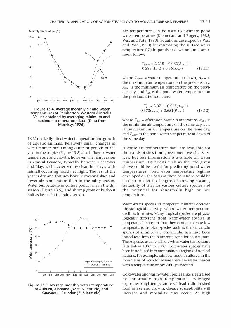
Water temperature in aquaculture ponds closely follows air temperatures, as shown in Figure 13.4, with data from Pemberton, Western Australia (Morrissy, 1976). The monthly air temperatures were about 0.5°C to 2.0°C higher than monthly water temperatures, but the trends of increase and decrease over the year were identical. It is widely recognized that the large seasonal changes in air temperature in temperate regions (Figures 13.4 and


13.5) markedly affect water temperature and growth of aquatic animals. Relatively small changes in water temperature among different periods of the year in the tropics (Figure 13.5) also influence water temperature and growth, however. The rainy season in coastal Ecuador, typically between December and May, is characterized by clear, hot days, with rainfall occurring mostly at night. The rest of the year is dry and features heavily overcast skies and lower air temperature than in the rainy season. Water temperature in culture ponds falls in the dry season (Figure 13.5), and shrimp grow only about half as fast as in the rainy season.

Air temperature can be used to estimate pond water temperature (Klemetson and Rogers, 1985; Wax and Pote, 1990). Equations developed by Wax and Pote (1990) for estimating the surface water temperature (°C) in ponds at dawn and mid-after-noon follow:

Tdawn = 2.218 + 0.062(Amax) + 0.285(Amin) + 0.561(Paft) (13.11)

where Tdawn = water temperature at dawn, Amax is the maximum air temperature on the previous day, Amin is the minimum air temperature on the previ-ous day, and Paft is the pond water temperature on the previous afternoon, and

Taft = 2.071 – 0.068(amin) + 0.373(amax) + 0.651(Pdawn) (13.12)

where Taft = afternoon water temperature, amin is the minimum air temperature on the same day, amax is the maximum air temperature on the same day, and Pdawn is the pond water temperature at dawn of the same day.

Historic air temperature data are available for thousands of sites from government weather serv-ices, but less information is available on water temperature. Equations such as the two given above could be useful for predicting pond water temperatures. Pond water temperature regimes developed on the basis of these equations could be used to predict the lengths of growing seasons, suitability of sites for various culture species and the potential for abnormally high or low temperatures.

Warm-water species in temperate climates decrease physiological activity when water temperature declines in winter. Many tropical species are physio-logically different from warm-water species in temperate climates in that they cannot tolerate low temperature. Tropical species such as tilapia, certain species of shrimp, and ornamental fish have been introduced into the temperate zone for aqua culture. These species usually will die when water temperature falls below 10°C to 20°C. Cold-water species have been introduced into mountainous regions of tropical nations. For example, rainbow trout is cultured in the mountains of Ecuador where there are water sources with a temperature below 20°C year-round.

Cold-water and warm-water species alike are stressed by abnormally high temperature. Prolonged exposure to high temperature will lead to diminished food intake and growth, disease susceptibility will increase and mortality may occur. At high

Figure 13.5. Average monthly water temperatures at Auburn, Alabama (32.5° N latitude) and

Guayaquil, Ecuador (2° S latitude)

Monthly temperature (°C)


Air

Water

Figure 13.4. Average monthly air and water temperatures at Pemberton, Western Australia.

Values obtained by averaging minimum and maximum temperature data. (Data from

Morrissy, 1976)


Wat

er t

emp

erat

ure

(°C

)

Guayaquil, EcuadorAuburn, Alabama


temperature, the respiration rate of the culture species and associated biota increases with high temperature and more dissolved oxygen is needed (Neill and Bryan, 1991).

Mean monthly air temperatures tend to be simi-lar from year to year, but temperature variation is much greater for shorter periods. Sudden episodes of cool weather can cause water temper-ature briefly to fall well below the monthly average and negatively impact survival and growth of aquaculture species. Szumiec (1981) observed that a difference of 1°C from the mean seasonal temperature may correspond to a differ-ence in carp production of 1 000 kg/ha in intensive systems.

Some farmers in the south-eastern United States produce tropical marine shrimp in inland ponds filled with water from saline aquifers. Shrimp post-larvae are stocked in the spring when water temperatures rise above 20°C. Cold fronts may pass through the region after shrimp have been stocked, causing water temperature to decline and stress or kill shrimp. Early stocking is essential because of the relatively short growing season for the tropical shrimp, but if stocked too early, a cold snap may kill the postlarvae. Shrimp also must be harvested in the fall before the onset of lethally low water temperatures.

Green and Popham (2008) estimated probabili-ties that a minimum air temperature less than or

equal to 14°C would last for one, three or five days during stocking and harvest seasons for inland shrimp in the United States. The critical temperature of 14°C was chosen because shrimp mortality was observed in ponds where water temperatures fell to 13.5°C–15.3°C for one night following a cold front in early October. Eight sites in the southern United States were identified and 100-year datasets of minimum air temperature were obtained from the United States National Oceanic and Atmospheric Administration. Probabilities for one of these sites, Greensboro, Alabama, are provided in Figure 13.6. At this loca-tion, the probability of a one-day period with water temperature below 14°C is less than 10 per cent only from mid-May until mid-September. Thus, the safest growing season for marine shrimp at Greensboro, Alabama, is only about 120 days. These probabilities can assist inland shrimp farm-ers to manage risk and refine management decisions at the beginning and end of the grow-ing season.

It has been observed that problems with low dissolved oxygen concentration in channel catfish culture in the south-eastern United States are frequently related to high temperature (Tucker, 1996). A worse scenario is a period of unusually hot days in summer followed by one or more calm, cloudy days. Under such conditions, dissolved oxygen concentrations will be low at a time when fish biomass, plankton abundance and feeding rate are high.

//

Mar Apr Apr May May Jun Sep Sep Oct Oct Oct Nov

Prob

abili

ty

1 day2 day3 day

1.0

0.8

0.6

0.4

0.2

0.0

Figure 13.6. Probabilities of a minimum air temperature of 14°C or less for 1 day and 3 or 5 consecutive days during the spring and fall in Greensboro, Alabama


Water temperature plays an important, indirect role in the health of aquatic animals because it strongly influences the occurrence and outcome of infectious diseases. The relationship between temperature and aquatic animal epizootics is complex because temperature affects both the host and pathogen, as well as other environmental factors that may influence host immunocompetence. These relation ships vary greatly among animal species and specific pathogens and by type of culture system. The immune system of aquatic animals generally functions most effectively at temperatures roughly corresponding to the range for best growth rate. At higher and lower temperatures, immunocompetence is diminished, while non-specific mediators of immunity are the primary means of preventing disease. Rapid temperature changes may also impair immune function, even if changes occur within the optimum range. Each pathogen also has an optimal temperature range for growth (or replication) and virulence, and it is the interaction between the effects of temperature on pathogen and host that determines the outcome of the epizootic. This interaction can lead to a pronounced seasonality of epizootics of certain diseases. For example, enteric septicaemia is the most important bacterial disease of pond-raised channel catfish. The disease is caused by the bacterium Edwardsiella ictaluri. Channel catfish are most susceptible to the disease when water temperatures range from 22°C to 28°C (Thune et al., 1993). In the catfish-growing areas of the south-eastern United States, pond water temperatures in that range typically occur in the spring and autumn, so there is a pronounced seasonal pattern of disease incidence. Pond waters are generally too cool to support disease outbreaks in the winter and too warm in the summer; major outbreaks of the disease occur primarily in the spring and autumn. There are many other examples for other species of increased incidence of disease during periods when the air and water temperatures are either rising or falling.

Water temperature is also a key factor in hatchery management and the production of aquatic animal larvae. The production of larvae for culture purposes often involves the inducement of ovula-tion and stimulation of milt production using exogenous hormones. While other environmental factors such as photoperiod and flow rate play a role, temperature is the crucial factor determining the rate of ovulation and milt production under natural and induced situations. Timing of this physiological reaction is related to the degree-hour response (water temperature multiplied by the number of hours from the onset of ovary matura-

tion, or dosing, until ovulation). Ovulation in common carp, Cyprinus carpio, requires 240 to 290 degree-hours, while in grass carp, Ctenopharyngodon idella, 205 to 215 degree-hours are required. The degree-hour response has been determined for several species (Horvath, 1978). Calculation of the time between administration of hormone and ovulation at 25°C for common carp is illustrated below:

Time to ovulation =

hours11.6 to9.6C25hoursC290

toC25hoursC240

°

°

°

°

=

(13.13)

Understanding the relationship between tempera-ture and mature gamete production and the associated effects is important for successful produc-tion of aquatic animal larvae.

13.5.3 Winterkill

Fish kills that occur in bodies of water with a winter ice cover are known as winterkill. When small water bodies are completely covered with ice and snow blankets the ice, light cannot penetrate into the water. There is no oxygen production by photosynthesis because of the lack of light, and respiration by organisms in the water and sedi-ment will cause the dissolved oxygen concentration to fall. The dissolved oxygen concentration will decline slowly because of the low temperature, but it is not replenished because the ice prevents re-aeration from the atmosphere. Dissolved oxygen depletion is most likely to occur in shal-low, eutrophic water bodies because they contain a large amount of organic matter and living biomass and have a small volume of water and a correspondingly small reserve of dissolved oxygen (Mathias and Barica, 1980).

Aquaculture ponds in cold regions are likely to experience winterkill because they receive large contributions of nutrients and organic matter and tend to be shallow. Snow removal from ice is one way of lessening the probability of winterkill. Another method is to aerate ponds to circulate water and prevent ice from covering the entire pond surface (Boyd, 1990). In more temperate climates, a brief period of unusually cold weather causing ice cover usually does not lead to winterkill.

13.5.4 Thermalstratification

Ponds and lakes stratify thermally because heat is absorbed more rapidly near the surface and the warm upper waters are less dense than cool lower waters (Table 13.5). Stratification occurs when


differences in the density of upper and lower strata become so great that the two layers cannot be mixed by wind. The classical pattern of thermal stratification of lakes in temperate zones is described by Wetzel (2001). At the spring thaw, or at the end of winter in a lake or pond without ice cover, the water column has a relatively uniform temperature. Heat is absorbed at the surface on sunny days, but there is little resistance to mixing by wind and the entire volume of water circulates and warms. As spring progresses, the surface water absorbs heat

more rapidly than heat can pass downward through the water column by conduction and mixing. The surface water becomes considerably warmer than deeper water.

The difference in density between the upper layer of water and the deeper water becomes so great that wind is no longer powerful enough to mix the two strata. The upper stratum is called the epilimnion and the lower stratum the hypolimnion. The stra-tum between the epilimnion and the hypolimnion

EPILIMNION Uniformlywarm water

Uniformlycold water

THERMOCLINE

Wind-driven water circulation

HYPOLIMNION

WATER TEMPERATURE ( °C )

20 3025 35

2

1

4

3

0

DEP

TH (

m)

AIR

Rapidly decreasing water temperature

Wind

Figure 13.7. Thermal stratification in a relatively deep pond

°C g cm–3 °C g cm–3 °C g cm–3

0 0.9998679 11 0.9996328 22 0.9977993

1 0.9999267 12 0.9995247 23 0.9975674

2 0.9999679 13 0.999404 0 24 0.9973256

3 0.9999922 14 0.9992712 25 0.9970739

4 1.0000000 15 0.9991265 26 0.9968128

5 0.9999919 16 0.9989701 27 0.9965421

6 0.9999681 17 0.9988022 28 0.9962623

7 0.9999295 18 0.9986232 29 0.9959735

8 0.9998762 19 0.9984331 30 0.9956756

9 0.9998088 20 0.9982323

10 0.9997277 21 0.9980210

Table 13.5. Density of freshwater at different temperatures (from Colt, 1984)


is termed the metalimnion or thermocline (Figure 13.7). Temperature changes at a rate of 1°C or more per metre of depth across the thermocline. The depth of the thermocline below the surface may fluctuate from less than 2 m to 10 m or more depending on the area, depth, turbidity and morphometry of water bodies and local weather conditions. Most larger lakes do not destratify until autumn. Air temperatures decline and heat is lost from the surface water to the air during autumn. The difference in density between upper and lower strata decreases until mixing finally causes the entire volume of water in the lake to circulate and destratify.

Tropical lakes also stratify. There are two annual maxima in solar radiation, but the variation in radiation flux is small, and factors other than solar radiation may be of major importance in regulating patterns of thermal stratification (Hutchinson, 1975; Wetzel, 2001). Large, shallow lakes in windy regions may not develop persistent stratification. At the other extreme, small, deep lakes may stratify and only destratify at irregular intervals of several years when abnormal cold spells occur. Most tropical lakes stratify, but destratification occurs one or more times annually as a result of wind, rain or changes in air temperature.

Ponds are shallower, more turbid, more protected from wind, and have a smaller surface area

than lakes. The ordinary warm-water fish pond seldom has an average depth of more than 2 m, a maximum depth of more than 4 or 5 m, and a surface area of more than a few hectares. Marked thermal stratification may develop even in shallow ponds, however, because turbid conditions result in rapid heating of surface waters on calm, sunny days.

The stability of stratification is determined by the amount of energy required to mix the entire volume of a body of water to a uniform temperature. The greater the energy required, the more stable the stratification. Aquaculture ponds are relatively small and quite shallow, and stratification is not as stable in them as it is in lakes and larger ponds. For exam-ple, 0.04 ha ponds with average depths of about 1 m and maximum depths of 1.6 to 1.8 m on the Fisheries Research Unit at Auburn, Alabama, will stratify ther-mally during daylight hours in warm months, only to destratify at night when the upper layers of water cool by conduction (Figure 13.8). Large, shallow aquaculture ponds (0.5–20 ha or more) stratify and destratify daily in the same manner.

Stratification and destratification of water bodies can be associated with biological activity and its effect on light penetration. A small, clear pond may stratify when a plankton bloom develops because the planktonic organisms suspended in the upper layer of water absorb heat and cause the upper layer of water to heat rapidly (Idso and Foster, 1974).

Water temperature (°C)

Dep

th (

m)

6 a.m. 3 p.m.

During later afternoon and night, air coolsand surface water cools until pond destratifies

Air

Water

During the day, air warms and surface water warms faster than deeper water

0.0

0.2

0.4

0.6

0.8

1.0

1.2

1.4

Figure 13.8. Daily thermal stratification and destratification in a shallow aquaculture pond


Light will penetrate deeper into the pond if the plankton bloom disappears, and destratification may occur.

13.5.5 Rainfallandwaterquality

Rain is normally acidic, for it is saturated with carbon dioxide. Pure water saturated with carbon dioxide has a pH of 5.6 (Boyd and Tucker, 1998). Rain more acidic than pH 5.6 contains a strong acid. Strong acids found in rainwater are formed by non-metallic oxides and hydrides of halogens. There are naturally occurring oxides of nitrogen, sulphur and chloride in the atmosphere. These can result in the formation of nitric acid, sulphuric acid and hydrochloric acid, respectively. In some areas, the natural background of strong acids can depress the pH of rainwater below 5.6. The combustion of fuels increases the concentration of nitrogen and sulphur compounds in the atmosphere and causes a marked depression in the pH of rainwater. In areas affected by heavy air pollution, the pH of rainwater may be below 4.

There are many reports, primarily from the north-eastern United States, eastern Canada and northern Europe, demonstrating the adverse effects of acid rain on aquatic ecosystems (Cowling, 1982). In regions where the acid-neutralizing capacity of soils and waters is low and rainfall is highly acidic, the pH and total alkalinity of lakes and streams has decreased. In the north-eastern United States and Canada, where the rainfall has a pH of 4.2 to 4.4 (Haines, 1981), many lakes and streams have declined in pH by 1 to 2 units during the last 30 to 40 years (Seip and Tollan, 1978). Many bodies of water in this region have a pH below 5.0 and aquatic organisms at all trophic levels have suffered adverse effects (Beamish and Harvey, 1972; Haines and Akielasek, 1983). Reproductive failures, skeletal deformities, reduced growth and even acute mortal-ity has been observed in fish populations (Haines, 1981).

The effects of acid rain on fish populations have been expressed mainly in areas where total alkalin-ity of surface waters is below 10 to 20 mg l–1 (Boyd and Tucker, 1998). Marine fisheries are unaffected by acid rain because coastal and oceanic waters are highly buffered. Freshwater aquaculture ponds with low-alkalinity water usually are treated with agri-cultural limestone (Boyd and Tucker, 1998), and this neutralizes the acidity from rain. Trout culture often is conducted in raceways, and the water source may be streams. There have been instances in North Carolina when runoff from heavy rainfall caused a sudden decline in the pH of stream water

supplying raceways and resulted in stress or death of trout.

Rain falling directly into ponds affects the surfaces by splashing water into the air and increasing the surface area for gas transfer. Depending upon the degree of oxygen saturation, dissolved oxygen concentrations may increase or decrease during a rainfall event. Night-time rainfall is more likely to increase dissolved oxygen concentration than daytime rainfall.

Erosion on watersheds during storm events may result in a turbid runoff that enters streams, ponds and other water bodies. Although coarse particles settle quickly, clay particles remain suspended for hours or days and create considerable turbidity. Settling particles can smother benthic organisms, and fish eggs that usually are deposited in depres-sions on the bottom can be destroyed by sediment. Prolonged turbidity reduces light penetration, less-ens primary productivity, and ultimately reduces fish production (Buck, 1956). Sediment accumula-tion in ponds also reduces depth and storage volume.

Ponds for production of marine species often are sited along estuaries and brackish water is pumped into them or sometimes introduced by tidal flow. Shellfish plots also are established in estuaries. The salinity at a given location in an estuary usually increases during rising tide and decreases with falling tide. Salinity also declines in response to increasing freshwater inflow. In tropical locations with distinct wet and dry seasons, salinity in coastal aquaculture ponds differs markedly between seasons (Figure 13.9). Large and medium-sized aquaculture projects are usually located at a place where the water is saline enough throughout the year. Small-scale projects are usually installed where space is available and little thought may be given to salinity, as other sites are unavailable.

Unusually heavy rainfall can cause extremely low salinity that stresses culture animals and leads to disease outbreaks or even causes direct mortality. Sometimes, heavy rainfall and associated runoff can cause rivers entering estuaries to change their course, which may affect aquaculture projects. Heavy rainfall during a cyclone at a shrimp farm in Madagascar caused a diversion in a river upstream of the farm to increase its catchment area and direct a greater flow of freshwater into the area where the pump station was located. Under the new hydro-logical conditions, the site of the pump station had freshwater continuously for two to three months


Figure 13.9. Relationship between rainfall and salinity in shrimp ponds near Guayaquil, Ecuador

during the year. This situation was unacceptable for shrimp culture, and therefore the pump station was moved to a more suitable location at considerable expense.

El Niño events result from increases in the temperature of the ocean by 1°C or 2°C above normal. El Niño events are rather common in the Western Pacific Ocean along the North and South American coasts. Between 1950 and 2004 there were 13 events, or an average of about one event every four years. Heavy rainfall during El Niño events causes low salinity that can stress or kill shrimp, but there also are benefits. The slightly warmer temperature of ocean waters may favour greater production by native fisher-ies and aquaculture operations. Increased rainfall and runoff also may flush pollution from estuar-ies that normally do not rapidly exchange water with the sea.

Blue-green algae excrete compounds into the water that impart an off-flavour to the flesh when adsorbed by fish and shrimp, which lowers market acceptability (Boyd and Tucker, 1998). Blue-green algae seldom are abundant in coastal shrimp ponds when salinity is below 10 parts per thousand (ppt). During the rainy season in tropical nations, salinity in shrimp ponds may decline below 10 ppt while blue-green algae abundance rises, resulting in an off-flavour (Boyd, 2003).

13.5.6 Wind

Wind creates waves on the water surface to increase the area for exchange of gases between air and water. Wind also mixes the water column, causing the movement of dissolved gases throughout a

water body. During the night and at other times when the dissolved oxygen concentration may be low, wind re-aeration is an important source of dissolved oxygen in ponds. When water is super-saturated with dissolved oxygen or other gases, however, wind action increases the rate of diffusion of gases into the air.

Boyd and Teichert-Coddington (1992) de oxygenated two ponds at the El Carao National Aquaculture Center, Comayagua, Honduras, by treatment with sodium sulphite and cobalt chloride; they also suppressed biological activity by application of formalin and copper sulphate. Wind speed, water temperature and dissolved oxygen concentration were monitored with a data logger system during the four-day re-aeration period. The wind re-aeration coefficient was calculated at intervals, and coefficients increased linearly (R2 = 0.88) with wind speed between 1 and 4.5 m s–1 (Figure 13.10). The regression equation was:

W = 0.153X – 0.127 (13.14)

where W = standard wind re-aeration coefficient for 20°C and 0.0 mg l–1 dissolved oxygen (g O2 m–2 h–1) and X = wind speed at 3 m height (m s–1). The following equation can be used to calculate the wind re-aeration rate for a specific pond:

K w = W Cs Cp

9.07 1.024T–20

(13.15)

where Kw = wind re-aeration rate (g O2 m–2 hr–1), Cs = dissolved oxygen concentration in pond water at saturation (g m–3), Cp = measured dissolved

Wind speed (m s–1)

Stan

dard

win

d re

-aer

atio

n co

effic

ient

(g m

2 h–

1 )

Figure 13.10. Regression of standard wind re-aeration coefficient on wind speed at a height

of 3 m above the pond water surface

Rain

fall

(cm

)

Month

Salin

ity (

ppt)

RainfallSalinity



oxygen concentration in pond (g m–3), and T = water temperature (°C).

Wind also creates water currents in ponds that are beneficial because they mix the water column, thus providing more uniform concentrations of dissolved oxygen to the bottom waters. In places where enhanced wind mixing is desirable, ponds can be constructed with their long axis parallel to the direc-tion of the prevailing wind. Wind-induced currents can resuspend sediment particles to create excessive turbidity and they can cause erosion of pond embankments. At sites where strong winds are common, vegetative barriers may be planted perpen-dicular to prevailing winds to provide wind-breaks. Moreover, stone or plastic liners may be installed along embankments to minimize wave erosion. Grass cover should be established on above- water portions of earthworks to protect against erosion by wind and rains (Boyd, 1999; Boyd et al., 2003).

When water in aquaculture ponds is still because of windless conditions, surface water often becomes highly supersaturated with dissolved oxygen. On bright, calm days, concentrations may exceed 200 per cent saturation (Boyd et al., 1994). Life stages of culture species or natural organisms that cannot move into deeper water to escape the excessive gas pressure near the surface may be stressed or killed by gas bubble trauma.

Strong winds or the combination of strong winds and heavy rainfall also may cause thermal destrati-fication of ponds and lakes during summer. The hypolimnion of eutrophic lakes and ponds is depleted of dissolved oxygen and has high concen-trations of dissolved and particulate organic matter, reduced iron and manganese, and other reduced inorganic and organic substances. When sudden destratification occurs, anaerobic hypolimnetic water dilutes the dissolved oxygen in the water with which it mixes. Oxygenation of reduced substances from the hypolimnion increases the oxygen demand. Cold fronts from the north-west some-times pass through the south-eastern United States in summer. These fronts travel quickly and result in strong winds and cold rain. Lakes and ponds in the region are typically stratified in summer and the mixing action of the wind and rain often causes destratification (FAO, 1968). Low dissolved oxygen concentration may occur in fertilized sport fish ponds and in commercial channel catfish ponds common in the region, and fish kills may result.

Cage culture operations commonly are placed in natural lakes or in reservoirs. These water bodies may thermally stratify, and the contribution of

wastes from cage culture operations will contribute to the oxygen demand in the hypolimnion. Sudden thermal destratification or overturns of lakes with cage culture operations can lead to dissolved oxygen depletion and massive fish mortality. For example, a large tilapia cage culture operation is located in El Cajon Reservoir in Honduras. In 2003, an unusu-ally strong cold front with heavy rain caused destratification of the reservoir. Dissolved oxygen concentrations declined to less than 0.5 mg l–1 in cages and there was a complete loss of the tilapia – the mortality was estimated at 1 500 tonnes of fish. An unknown quantity of wild fish in the reservoir also died. Similar mass mortalities of fish resulting from thermal overturns of lakes with cage culture operations have also been reported in Indonesia, the Philippines, China and other countries (Schmittou, 1993).

Ponds for shrimp farming and other types of coastal aquaculture are especially susceptible to storm damage. There have been numerous cases in which ponds have been overtopped by storm surges and embankments have been breached. One of the most disastrous examples was the impact of Hurricane Mitch on shrimp farms along the Gulf of Fonseca in Honduras and Nicaragua in 1998. Heavy rainfall from the hurricane caused extensive flooding that overtopped and breached embankments and left deep layers of sediment in riverbeds, canals and ponds. Mangroves provide considerable protection from waves and storm surges. In some locations, the likelihood of storm damage has been exacerbated by the removal of mangrove forest for constructing ponds. Shrimp and other aquaculture farms should be constructed behind mangrove areas with the mangrove habitats left undisturbed (Phillips, 1995).

In regions where hurricanes are frequent, farms should be designed to minimize damage by taking into account probable storm surge height and wind velocities. These precautions are seldom considered, but farm managers usually lower water levels in ponds so that rain falling into ponds does not cause water to overtop embankments.

Aquaculture cages are especially susceptible to heavy waves. There have been numerous instances of escapes of culture species as a result of cage failure in storms (FAO, 1984). Such events are obviously economically damaging to producers, but there are also environmental concerns related to escapes. Some scientists think that farmed fish are genetically inferior to wild stocks, and massive escapes from cages or other facilities could damage the gene pools of local populations of the same species. Cages should be installed in areas that are less susceptible


to heavy waves. Recent advances in cage technology have reduced the probability of cage failure. Some cages are even installed several metres below the surface to minimize the influence of heavy seas.

13.5.7 Barometricpressure

Dissolved oxygen concentration is probably the single most important variable in aquaculture. This parameter is frequently measured in ponds for research and commercial aquaculture. The usual method of measurement is a polarographic dissolved oxygen meter. In order to properly calibrate a dissolved oxygen meter or to estimate the dissolved oxygen concentration at saturation in a body of water, the barometric pressure must be known. The most common source of barometric pressure infor-mation is a weather station at the nearest airport. Individuals using such data should be aware that barometric pressure readings at these stations usually have been adjusted to the equivalent pressure at sea level. The station barometric pressure is needed for calibrating dissolved oxygen meters or estimating dissolved oxygen concentration at saturation. Boyd (1990) provided instructions and tabular data needed for correcting sea-level-adjusted barometric pressure readings to station barometric pressures.

Data for dissolved oxygen concentration at satura-tion (Table 13.4) are for sea level. These values can be adjusted to station barometric pressure with the following equation:

OD ss = DOssl BP760 (13.16)

where DOss = dissolved oxygen saturation at station (mg l–1); DOssl = dissolved oxygen saturation at sea level (mg l–1); BP = station barometric pressure (mm hg).

If barometric pressure cannot be measured but station elevation is known, the barometric pressure can be estimated by the following equation (Colt, 1984):

log10 BP = 2.880 814 Station elevation (m)19 748.2

(13.17)

13.6 RESEARCHNEEDS

There needs to be a more organized effort to define relationships between agrometeorological data and fisheries and aquacultural production. In fisheries, the greatest priority probably should be given to predicting the influence that global climate change will have on production. Of course, a better understanding of the influence of meteorological

variables on the structure and function of natural aquatic ecosystems should also be a long-term goal. Better methods for predicting the forces, paths and conditions of storms and enhanced communications for warning fishermen of impending danger could save many lives.

In aquaculture, the emphasis should be placed on developing a greater knowledge of the relationships among agrometeorological variables, water quality and production. Some particularly important issues include the effects of wind-induced circulation on water quality, phytoplankton and off-flavour in ponds; refinement of dissolved oxygen models to incorporate weather forecast information and newer technologies for measuring phytoplankton biomass, such as satellite images and hand-held spectral reflec-tometers; predictive models of fish feeding behaviour based on weather and water quality data; and effects of weekly or shorter variations in water temperature on the growth of culture species.

Much of the inland aquaculture in developing nations is done in ponds without the option for mechanical aeration. Sites with good exposure to the wind are favoured, and periods of calm, hot weather are potentially dangerous to fish popula-tions. In areas with a high probability of calm weather, production levels should be lowered so that phytoplankton blooms do not become exces-sive and cause chronically low night-time dissolved oxygen concentrations.

There are millions of hectares of aquaculture ponds in the world, and most of them are concentrated in Asia. Compared to natural aquatic ecosystems, large amounts of nutrients are applied to these ponds, and organic matter accumulates in pond bottoms (Boyd and Tucker, 1998). Decomposition of organic matter in sediment of aquaculture ponds produces carbon dioxide and methane that enter the atmosphere. It would be interesting to determine the contribution of world aquaculture to greenhouse gases.

Global warming will affect aquaculture production. Because aquaculture will eventually be the main source of fisheries products, it seems imperative to assess the possible negative impacts of global warm-ing on the major types of aquaculture.

13.7 APPLICATIONOFAGROMETEOROLOGY

Existing meteorological and climatological data should be more fully used in fisheries and


aqua culture. Aquaculturists need to be aware of local conditions relating to normal patterns in air temperature, solar radiation, cloud cover, evaporation and wind velocity. A knowledge of the frequency of excessive rainfall and floods, droughts, air temperatures that are lower or higher than normal, and destructive storms would also be beneficial. Armed with this information, aquaculturists would be able to plan and conduct operations in harmony with local climatic conditions. Aquaculturists could use local weather forecasts to prepare for adverse weather and decrease the likelihood of weather- related losses.

Aquaculture is a major activity in many nations, and it is expected to expand in the future. Because of increasing environmental awareness and the need to conserve natural resources, environmental impact analysis (EIA) often is required for new commercial aquaculture projects (Boyd and Tucker, 1998). An EIA should include an evaluation of local climate and adverse weather conditions that could affect the project. The size of the project should be in accord-ance with the availability of water and facilities should be designed to protect against drought, flood-ing, wind and water erosion, and storms.

Conservation of freshwater is a major issue worldwide. It is particularly important to design aquaculture facilities so that water can be used efficiently (Boyd, 2005). An effort should be made in major aquaculture regions to provide the aquaculture sector with records of rainfall (to include frequency–intensity–duration relationships for use in the design of facilities) and evaporation.

13.8 EDUCATIONNEEDS

The major obstacle to the use of agrometeorological data in fisheries and aquaculture is the lack of famili-arity with the topic by those who work in the sector. The training of aquaculture scientists does not

usually include coursework in this area. The impor-tance of water temperature is included in courses about aquaculture production, but the relationship of water temperature to other agrometeorological data is usually not emphasized. Even less attention is given to precipitation, evaporation, wind and other meteorological variables in the training of aqua-culture scientists. This is a strange situation and is probably the result of the development of aqua-culture curricula within fisheries or biology programmes, where the emphasis has been on natu-ral systems that are not managed intensively. In agronomy, all students are required to take at least one basic soil science course that includes informa-tion on the interaction of climatic factors with soils and their productivity. A similar class in water science should be provided to students of fisheries and aquaculture. This kind of class is currently being taught at Auburn University in the United States. It includes information on meteorology, hydrology and water quality, with emphasis on how these topics are related to fisheries and aquaculture.

Nations with large aquaculture sectors have exten-sion programmes to provide technical assistance to producers. Governmental fisheries agencies in these countries usually are in close contact with interna-tional development organizations such as FAO, the World Bank and the Asian Development Bank, and foreign aid programmes from Australia, Canada, the European Union, Japan and the United States. These development organizations should be made aware of the importance of agrometeorological data in aquaculture and fisheries so that they can initi-ate training efforts and provide data to producers. The most effective way of promoting the use of agrometeorological data in aquaculture is to convince the future generation of fisheries and aquacultural scientists that these data are useful and to train them to use the data. They will then begin to conduct research on the topic and include information about agrometeorology in their exten-sion programmes. As a result, those who work in the private sector as managers will apply agromete-orological data to farm operations.

REFERENCES

Abeliovich, A., D. Kellenberg and M. Shilo, 1974: Effects of photo-oxidative conditions on levels of superoxide dimutase in Anacystis nidulans. J. Photochem. Photobiol., 19:379–382.

Abeliovich, A. and M. Shilo, 1972: Photo-oxidative death in blue-green algae. J. Bacteriol., 11:682–689.

Almazan, G. and C.E. Boyd, 1978: An evaluation of Secchi disk visibility for estimating plankton density in fish ponds. Hydrobiologia, 61:205–208.

Amir, I., J.B. Arnold and W.K. Bilanski, 1977: A procedure for determining probabilities of dry and wet days. Can. Agric. Eng., 19:2–5.

Beamish, R. and H. Harvey, 1972: Acidification of the LaCloche Mountain Lakes, and resulting fish mortalities. J. Fish. Res. Board Can., 29:1131–1143.

Bolte, J.P., S.S. Nath and D.H. Ernst, 1995: POND: A decision support system for pond aquaculture. In: Twelfth Annual Administrative Report. Corvallis, Pond Dynamics/Aquaculture Collaborative Research Support Program, Oregon State University.

Boyd, C.E., 1982: Hydrology of small experimental fish ponds at Auburn, Alabama. Trans. Am. Fish. Soc., 111:638–644.

———, 1985: Pond evaporation. Trans. Am. Fish. Soc., 114:299–303.

———, 1986: Influence of evaporation excess on water requirements for fish farming, In: Proceedings of the Conference on Climate and Water Management – A Critical Era. Boston, American Meteorological Society.

———, 1990: Water Quality in Ponds for Aquaculture. Auburn, Alabama Agricultural Experiment Station, Auburn University.

———, 1999: Codes of Practice for Responsible Shrimp Farming. St Louis, Global Aquaculture Alliance.

———, 2003: Off-flavor in pond-cultured marine shrimp, In: Off-flavors in Aquaculture (A.M. Rimando and K.K. Schrader, eds). Washington, DC, American Chemical Society.

———, 2005: Water use in aquaculture. World Aquaculture, 36(3):12–15 and 70.

Boyd, C.E., J.A. Davis and E. Johnston, 1978a: Die-offs of the blue-green alga, Anabaena variabilis, in fish ponds. Hydrobiologia, 61:129–133.

Boyd, C.E. and A. Gross, 2000: Water use and conservation for inland aquaculture ponds. Fish. Manag. Ecol., 7:55–63.

Boyd, C.E., E.E. Prather and R.W. Parks, 1975: Sudden mortality of massive phytoplankton bloom. Weed Sci., 23:61–67.

Boyd, C.E., J.F. Queiroz, G.N. Whitis, R. Hulcher, P. Oakes, J. Carlisle, D. Odom Jr, M.M. Nelson and W.G. Hemstreet, 2003: Best Management Practices for Channel Catfish Farming in Alabama. Special Report 1. Montgomery, Alabama Catfish Producers.

Boyd, C.E., R.P. Romaire and E. Johnston, 1978b: Predicting early morning dissolved oxygen concentrations in channel catfish ponds. Trans. Am. Fish. Soc., 107:484–492.

Boyd, C.E. and J.L. Shelton Jr, 1984: Observations on the Hydrology and Morphometry of Ponds on the Auburn University Fisheries Research Unit. Bulletin 558. Auburn, Alabama Agricultural Experiment Station, Auburn University.

Boyd, C.E. and D. Teichert-Coddington, 1992: Relationship between wind speed and re-aeration in small aquaculture ponds. Aquacult. Eng., 11:121–131.

Boyd, C.E. and C.S. Tucker, 1998: Pond Aquaculture Water Quality Management. Boston, Kluwer Academic Publishers.

Boyd, C.E., B.J. Watten, V. Goubier and R. Wu, 1994: Gas supersaturation in surface waters of aqua-culture ponds. Aquacult. Eng., 13:31–39.

Buck, D.H., 1956: Effects of turbidity on fish and fishing. Trans. North Am. Wildl. Conf., 21:249–261.

Colt, J., 1984: Computation of Dissolved Gas Concentrations in Water as Functions of Temperature, Salinity, and Pressure. Special Publication No. 14. Bethesda, American Fisheries Society.

Cowling, E.B., 1982: Acid precipitation in historical perspective. J. Environ. Sci. Tech., 16:110–123.

Doyle, K.M. and C.E. Boyd, 1984: The timing of inorganic fertilization of sunfish ponds. Aquaculture, 37:169–177.

Farnsworth, R.K. and E.S. Thompson, 1982: Mean Monthly, Seasonal, and Annual Pan Evaporation for the United States. NOAA Technical Report NWS 34. Washington, DC, United States Department of Commerce.

Fogg, G.E. and A.E. Walsby, 1971: Buoyancy regula-tion and growth of planktonic blue-green algae. Mitt. Internat. Verein. Limnol., 19:182–188.

Food and Agriculture Organization of the United Nations (FAO), 1968: Fish kills caused by


phytoplankton blooms and their prevention. Proceedings of the World Symposium on Warm-Water Pond Fish Culture (H.S. Swingle, ed.). Fisheries Report No. 44, Vol. 5. Rome, FAO.

———, 1984: Cage and Pen Fish Farming (M.C.M. Beveridge). Fisheries Technical Paper No. 255. Rome, FAO.

Green, B.W. and T.W. Popham, 2008: Probabilities of low nighttime temperatures during stocking and harvest seasons for inland shrimp culture. J. World Aquacult. Soc., 39:91–103.

Haines, T.A., 1981: Acid precipitation and its conse-quences for aquatic ecosystems: A review. Trans. Am. Fish. Soc., 110:669–707.

Haines, T.A. and J.J. Akielasek, 1983: Acidification of headwater lakes and streams in New England. In: Lake Restoration, Protection, and Management. EPA 440/5-83-001. Washington, DC, United States Environmental Protection Agency.

Hanson, T. and C. Hogue, 2001: Effects of drought on commercial catfish production in Mississippi. Catfish Journal, Jan. 2001:8–10.

Horvath, L., 1978: Relation between ovulation and water temperature by farmed cyprinids. Aquaculture Hungarica, 1:58–65.

Hutchinson, G.W., 1975: A Treatise on Limnology. Vol. III. Limnological Botany. New York, John Wiley and Sons.

Idso, S.B. and J.M. Foster, 1974: Light and tempera-ture relations in a small desert pond as influenced by phytoplankton density variations. Water Resources Research, 10:129–132.

Idso, S.B. and R.G. Gilbert, 1974: On the universal-ity of the Poole and Atkins Secchi disk-light extinction equation. J. Appl. Ecol., 11:399–401.

Kapetsky, J.M., 2000: Present applications and future needs of meteorological and climatologi-cal data in inland fisheries and aquaculture. Agric. For. Meteorol., 103:109–117.

Klemetson, S.L. and G.L. Rogers, 1985: Aquaculture pond temperature modeling. Aquacult. Eng., 4:191–208.

Langbein, W.B., 1967: Hydroclimate. In: The Encyclopedia of Atmospheric Sciences and Astrogeology (R.W. Fairbridge, ed.). New York, Reinhold Publishing.

Mathias, J.A. and J. Barica, 1980: Factors controlling oxygen depletion in ice-covered lakes. Can. J. Fish. Aquat. Sci., 37:185–194.

McConnell, W.J., 1963: Primary productivity and fish harvest in a small desert impoundment. Trans. Am. Fish. Soc., 92:1–12.

Meteorological Department of Thailand, 1981: Climatological Data of Thailand 30-year Period (1951–1980). Bangkok, Ministry of Communications.

Morrissy, N.M., 1976: Aquaculture of marron, Cherax tenuimanus (Smith). Part 1. Site selection and the potential of marron for aquaculture. Fish. Res. Bull. West. Aust., 17:1–27.

Neill, W.H. and J.D. Bryan, 1991: Responses of fish to temperature and oxygen, and response inte-gration through metabolic scope. In: Advances in World Aquaculture. Vol. 3. Aquaculture and Water Quality (D.E. Brune and J.R. Tomasso, eds). Baton Rouge, World Aquaculture Society.

Phillips, M.J., 1995: Shrimp culture and the envi-ronment. In: Towards Sustainable Aquaculture in Southeast Asia and Japan (T.U. Begarinao and E.E.C. Flores, eds). Iloilo, SEAFDEC Aquaculture Department.

Romaire, R.P. and C.E. Boyd, 1979: Effects of solar radiation on the dynamics of dissolved oxygen in channel catfish ponds. Trans. Am. Fish. Soc., 108:473–478.

Schmittou, H.R., 1993: High Density Fish Culture in Low Volume Cages. Singapore, South Asia Office, American Soybean Association.

Schoof, R.R. and G.A. Gander, 1982: Computation of runoff reduction caused by farm ponds. Water Resources Bulletin, 18:524–532.

Seip, H. and A. Tollan, 1978: Acid precipitation and other possible sources of acidification of rivers and lakes. Sci. Tot. Environ., 10:253–270.

Silapajarn, O. and C.E. Boyd, 2005: Effects of chan-nel catfish farming on water quality and flow in an Alabama stream. Rev. Fish. Sci., 13:109–140.

Szumiec, M.A., 1981: The dependence of carp growth rate on temperature. Gosp. Rybna, 2:4–7.

———, 1983: Meteorology in the service of limnol-ogy and aquaculture, Polskie Archiwum Hydrobiologii (Pol. Arch. Hydrobiol.), 30(1):5–13.

Thune, R.L., L.A. Stanley and R.K. Cooper, 1993: Pathogenesis of gram-negative bacterial diseases in warmwater fish. Annu. Rev. Fish Dis., 3:37–68.

Tucker, C.S., 1996: The ecology of channel catfish ponds in northwest Mississippi. Rev. Fish. Sci., 4:1–55.

United States Soil Conservation Service (USSCS), 1972: Hydrology. In: SCS National Engineering Handbook. Washington, DC, USSCS, United States Government Printing Office.

———, 1979: Ponds and Reservoirs. In: SCS Engineering Field Manual. Washington, DC, USSCS, United States Government Printing Office.

Wallis, A.L. Jr, 1977: Comparative Climatic Data through 1976. Asheville, United States Department of Commerce, NOAA, Environmental Data Service, National Climatic Center.

Wax, C.L. and J.A. Pote, 1990: A derived climatol-ogy of water temperatures for the Mississippi


catfish industry. J. World Aquacult. Soc., 21:25–34.

Wetzel, R.G., 2001: Limnology. Third edition. San Diego, Academic Press.

World Meteorological Organization, 1973: Comparisons between Pan and Lake Evaporation (C.E. Hounam) (WMO-No. 354), Geneva.

Yoo, K.H. and C.E. Boyd, 1994: Hydrology and Water Supply for Aquaculture. New York, Chapman and Hall.

Zagarese, H. and C.E. Williamson, 2001: The implications of solar UV radiation exposure for fish and fisheries. Fish and Fisheries, 2:250–260.

APPLICATION OF AGROMETEOROLOGY TO AQUACULTURE AND · PDF file ·...

Documents

Transcript of APPLICATION OF AGROMETEOROLOGY TO AQUACULTURE AND · PDF file ·...