Ai

J

fcplga

m

©

GEOPHYSICS, VOL. 72, NO. 5 �SEPTEMBER-OCTOBER 2007�; P. J53–J64, 13 FIGS., 1 TABLE.10.1190/1.2761848

pplication of a new 2D time-domain full-waveformnversion scheme to crosshole radar data

acques R. Ernst1, Alan G. Green1, Hansruedi Maurer1, and Klaus Holliger2

ta5

sv�BaPdfpW

epem�1Cet2�eotbt

maaa

eceivedich, Sw

usanne

ABSTRACT

Crosshole radar tomography is a useful tool in diverse in-vestigations in geology, hydrogeology, and engineering.Conventional tomograms provided by standard ray-basedtechniques have limited resolution, primarily because only afraction of the information contained in the radar data �i.e.,the first-arrival times and maximum first-cycle amplitudes� isincluded in the inversion. To increase the resolution of radartomograms, we have developed a versatile full-waveform in-version scheme that is based on a finite-difference time-do-main solution of Maxwell’s equations. This scheme largelyaccounts for the 3D nature of radar-wave propagation and in-cludes an efficient method for extracting the source waveletfrom the radar data. After demonstrating the potential of thenew scheme on two realistic synthetic data sets, we apply it totwo crosshole field data sets acquired in very different geo-logic/hydrogeologic environments. These are the first appli-cations of full-waveform tomography to observed crossholeradar data. The resolution of all full-waveform tomograms isshown to be markedly superior to that of the associated ray to-mograms. Small subsurface features a fraction of the domi-nant radar wavelength and boundaries between distinct geo-logical/hydrological units are sharply imaged in the full-waveform tomograms.

INTRODUCTION

Crosshole radar methods are capable of providing reliable subsur-ace tomographic images of dielectric permittivity ��� and electricalonductivity ���. These two properties are intimately linked to im-ortant local hydrogeological conditions, salinity, clay content, andithological variations. Acquisition of crosshole radar data involvesenerating high-frequency electromagnetic pulses �20–250 MHz�t numerous locations along one borehole and then recording the

Manuscript received by the Editor February 16, 2007; revised manuscript r1Swiss Federal Institute of Technology, Institute of Geophysics, Zur

aurer@aug.ig.erdw.ethz.ch.2University of Lausanne, Faculty of Earth and Environmental Sciences, La2007 Society of Exploration Geophysicists.All rights reserved.

J53

ransmitted and scattered waves at a large number of positions alongsecond borehole. The pulses have dominant wavelengths of

.0 to 0.4 m in the subsurface.The vast majority of published tomographic radar images of the

hallow subsurface have been derived from standard ray-based in-ersions of first-arrival times and maximum first-cycle amplitudese.g., Olsson et al., 1992; Carlsten et al., 1995; Fullagar et al., 2000;ellefleur and Chouteau, 2001; Tronicke et al., 2001, 2004; Irvingnd Knight, 2005; Clement and Barrash, 2006; Musil et al., 2006;aasche et al., 2006�. Unfortunately, the resolution provided by stan-ard ray tomography is limited by the relatively small amount of in-ormation included in the inversion — resolution scales with ap-roximately the diameter of the first Fresnel zone �Williamson andorthington, 1993�.To improve the resolution and interpretability of subsurface imag-

s provided by radar methods, a number of waveform-type ap-roaches have been developed over the past two decades.Approach-s have included approximate Born �weak-scattering� iterativeethods based on integral representations of Maxwell’s equations

Wang and Chew, 1989; Chew and Wang, 1990; Sena and Toksöz,990; Moghaddam et al., 1991; Moghaddam and Chew, 1992, 1993;ui et al., 2001� and the approximate wave-equation traveltime �Cait al., 1996�, Fresnel-volume �Johnson et al., 2005�, and diffraction-omography methods �Cui and Chew, 2000, 2002; Zhou and Liu,000; Cui et al., 2004�. More exact full-waveform techniquesMoghaddam et al., 1991; Jia et al., 2002; Ernst et al., 2005; Kurodat al., 2005; Ernst et al., 2007� have also been described. Almost allf these waveform-type approaches have only been tested on syn-hetic data and not applied to recorded crosshole radar data. A nota-le exception is Cai et al. �1996� who apply their wave-equation-raveltime method to observed first-arrival traveltimes.

We have recently introduced a 2D time-domain full-waveform to-ographic scheme for the inversion of crosshole radar data �Ernst et

l., 2005, 2007�. Our intention here is to demonstrate its potentialnd limitations via applications to two realistic synthetic data setsnd two field data sets, one acquired within a relatively dry grano-

May 18, 2007; published onlineAugust 23, 2007.itzerland. E-mail: jack@aug.ig.erdw.ethz.ch; alan@aug.ig.erdw.ethz.ch;

, Switzerland. E-mail: klaus.holliger@unil.ch.

dwRfdstt

wpfArsfrc

tmahotMG2w�Kfdmwm

imn�ttugbfib�

RddFaqJ

scdT

sF

1

2

3

4

5

6

7

8

9

1

1

1

1

Dp

b��Tigct

oteg

J54 Ernst et al.

ioritic rock mass �Grimsel Rock Laboratory� and one recordedithin a water-saturated alluvial aquifer �Boise Hydrogeophysicalesearch Site�. To our knowledge, these are the first applications of

ull-waveform tomographic inversion to observed crosshole radarata. In contrast to waveform-type investigations that only involveynthetic data, it is necessary with field data to account for the 3D na-ure of wave propagation through the probed media and to estimatehe source wavelet.

After briefly reviewing the principal features of the new full-aveform tomographic inversion scheme, we summarize key im-lementation details. Although it is essential to account for 3D ef-ects and estimate the source wavelet, these issues are discussed inppendices A and B to maintain continuity of the main text. In the

emainder of the paper, we present the results of applying the newcheme to the synthetic and field data sets. In each case, full-wave-orm tomograms are compared to the corresponding conventionalay tomograms to illustrate the advantages of our more elaborate andomplete approach.

FULL-WAVEFORM INVERSION

Since Tarantola’s �1984a, b, 1986� pioneering papers appeared onhe full-waveform inversion of seismic data, numerous inversion

ethods have been developed and applied to seismic data generatednd recorded at the surface and/or along boreholes. These methodsave included finite-difference and finite-element approaches basedn representations of the acoustic-, elastic-, viscoelastic-, and aniso-ropic-wave equations in both the time and frequency domains �e.g.,

ora, 1987, 1988; Pica et al., 1990; Pratt, 1990a, b, 1999; Zhou andreenhalgh, 1998a, 2003; Pratt and Shipp, 1999; Watanabe et al.,004; Sinclair et al., 2007�. Comparable developments on the full-aveform inversion of radar data have been much more limited

Moghaddam et al., 1991; Jia et al., 2002; Ernst et al., 2005, 2007;uroda et al., 2005�. In this contribution, we employ our new 2D

ull-waveform tomographic inversion scheme to synthetic and fieldata. Details on the mathematical formulations and computer imple-entation of this scheme are provided by Ernst et al. �2007�. Here,e describe only the most important theoretical and numerical ele-ents.For the forward modeling of electromagnetic waves propagating

n heterogeneous media, we employ a 2D finite-difference time-do-ain �FDTD� solution of Maxwell’s equations in Cartesian coordi-

ates. For the inverse component, we modify and extend Tarantola’s1984a� approach to operate in the electromagnetic wave regime. Inypical borehole radar configurations, we are primarily interested inhe electric field component parallel to the borehole axis; hence wese TE mode equations. These equations are solved using staggered-rid finite-difference operators that are second-order accurate inoth time and space �Taflove and Hagness, 2000�. Application of ef-cient generalized perfectly matched layer �GPML� absorbingoundaries minimizes artificial reflections from the model edgesFang and Wu, 1996�.

During the inversion, a conjugate-gradient technique �Polak andibière, 1969� is used to find the minimum of a cost functional thatefines the differences between the observed and model-predictedata. An adjoint method determines the update gradient directions.urthermore, an algorithm described by Pica et al. �1990� suppliesn optimum estimate of the step size at each iteration. As a conse-uence, we avoid computationally expensive calculations of theacobian matrix.

Before applying our 2D full-waveform tomographic inversioncheme, there are two tasks. First, we need to account �as best wean� for the 3D characteristics of wave propagation through the me-ia. Second, we must determine an estimate of the source wavelet.hese two critical tasks are discussed inAppendicesAand B.Implementation of our full-waveform tomographic inversion

cheme involves the following 13 steps �see Ernst et al., 2007 andigure B-2�:

� Apply preinversion data processing to reduce high-frequencynoise. Mitigate the effects of out-of-plane energy. �Transform�the crosshole radar data to 2D �seeAppendix A�.

� Invert the first-arrival times and maximum first-cycle ampli-tudes using standard ray-based tomography.

� Convert the ray velocity and attenuation tomograms to initial �and � models.

� Compute a synthetic wavefield using the initial � and � conduc-tivity models and a rough estimate of the source wavelet �boxes1 and 2 in Figure B-2�.

� Determine a realistic estimate of the source wavelet using thedeconvolution method outlined in Appendix B �boxes 3 to 5 inFigure B-2�.

� Compute the synthetic wavefield using the model parametersand the realistic source-wavelet estimate determined at step 5.

� Subtract the synthetic data from the observed data to determinethe residual wavefield.

� Compute the cost functional S = 0.5�E − Eobs�2, where E is themodel-predicted data and Eobs is the observed data.

� Use the same model parameters employed at step 6 and the re-sidual wavefield to generate the back-propagated syntheticwavefield �i.e., the residual wavefield at all receiver locations issimultaneously back-propagated�.

0� Calculate the inversion update directions by crosscorrelatingthe forward- and back-propagated wavefields.

1� Determine the step length that provides fast, yet stable and ac-curate, inversions.

2� Update the � and � models using the derived gradient directionand step length.

3� Repeat steps 5–12 until convergence is achieved �i.e., until thechange in root-mean-square �rms� difference between the actu-al and model-predicted data is below 1%�.

uring the inversion, the complete wavefield only needs to be com-uted three times per iteration �i.e., steps 6, 9, and 11�.

Our attempts to invert simultaneously for � and � fail primarilyecause of the large differences between the magnitudes of the � andFréchet derivatives, even though they are not explicitly calculated

Watanabe et al. �2004� discuss the equivalent acoustic problem�.his problem can be circumvented. First, we invert for � while keep-

ng � fixed. Then, we invert for � while keeping � fixed �i.e., one sin-le computational cycle; Ernst et al., 2007�. Although this sequencean be repeated until convergence is achieved, only a single compu-ational cycle is required for all examples presented in this article.

APPLICATION TO REALISTIC SYNTHETIC DATA

In the following section, we explore the potential and limitationsf our full-waveform inversion scheme using two very similar syn-hetic data sets, one pure 2D and the other quasi-3D �other syntheticxamples are presented in Ernst et al., 2007�. The two data sets areenerated using the same medium parameters, borehole geometries,

aFmsa�=trTg11

1hT00

g�nfiw

Swt

alueTtFt

btbUmstv

T

�

Fdc�=0ifFla

2D waveform inversion of radar data J55

nd boundaries of the stochastic models �Table 1, Figure 1a and d�.or convenience, the models are expressed in terms of relative per-ittivity �r = �/�0, where �0 is the dielectric permittivity of free

pace. Average or background medium properties are �rmean = 10.3

nd � mean = 1.4 mS/m and the stochastic variations are defined by1� exponential covariance functions with standard deviations �r

std.

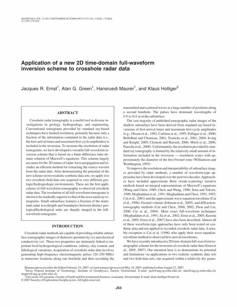
0.8 and �std. = 1.7 mS/m and �2� horizontal and vertical correla-ion lengths of 2.0 and 0.2 m, respectively. Figure 1a and d show theesultant �r and � distributions used to generate the synthetic data.he distributions have distinct subhorizontal fabrics, with zones ofenerally low �r and low � within 1 m of the surface and below6-m depth, and a zone of mostly high �r and high � between 4- and0-m depth.

The two 20-m-deep boreholes in our models are separated by0 m, with 41 equally spaced transmitter antennas in the left bore-ole and 41 equally spaced receiver antennas in the right borehole.he grid spacings used for the forward and inverse computations are.02 and 0.06 m, and the model space is surrounded by a.8-m-thick GPML frame.

We employ an FDTD algorithm in 2D Cartesian coordinates toenerate the true 2D noise-free data for the first synthetic experimentsynthetic I in Table 1� and an FDTD algorithm in cylindrical coordi-ates �Ernst et al., 2006� to generate the pseudo-3D noise-free dataor the second experiment �synthetic II in Table 1�. The source signaln both experiments is a 100 MHz Ricker wavelet that yields signalsith �1 m dominant wavelengths in the models.

ynthetic experiment I: Determining the sourceavelet and distributions of � and � from

rue 2D synthetic data

Conventional ray-based inversions of the first-arrival traveltimesnd maximum first-cycle amplitudes provide electromagnetic ve-ocity and attenuation tomograms. These tomograms are convertedsing relatively standard high-frequency relationships �Holligert al., 2001� to the �r and � ray tomograms shown in Figure 1b and e.he �r ray tomogram is a somewhat blurred image that well portrays

he important broad-scale zoning of the original model �compareigure 1a and b�, but the � ray tomogram is a rather poor representa-

ion of the original model �compare Figure 1e and d�.Despite the shortcomings of the two ray tomograms, they are the

able 1. Summary of model parameters. Homogeneous initial

Experiments

Model widthand depth

�m�

Number oftransmitters/

receivers

I

��r

Synthetic I�Figures 1, 2a, and 3�

10 and 20 41/41 �rmean

stocwith sof �r

st

and cof x =

Synthetic II�Figures 2b and 4�

10 and 20 41/41

GrimselFigures 5, 6, 7a, and 8�

10 and 20 41/40

Boise�Figures 7b and 9–11�

8.5 and 20 77/40�see main text�

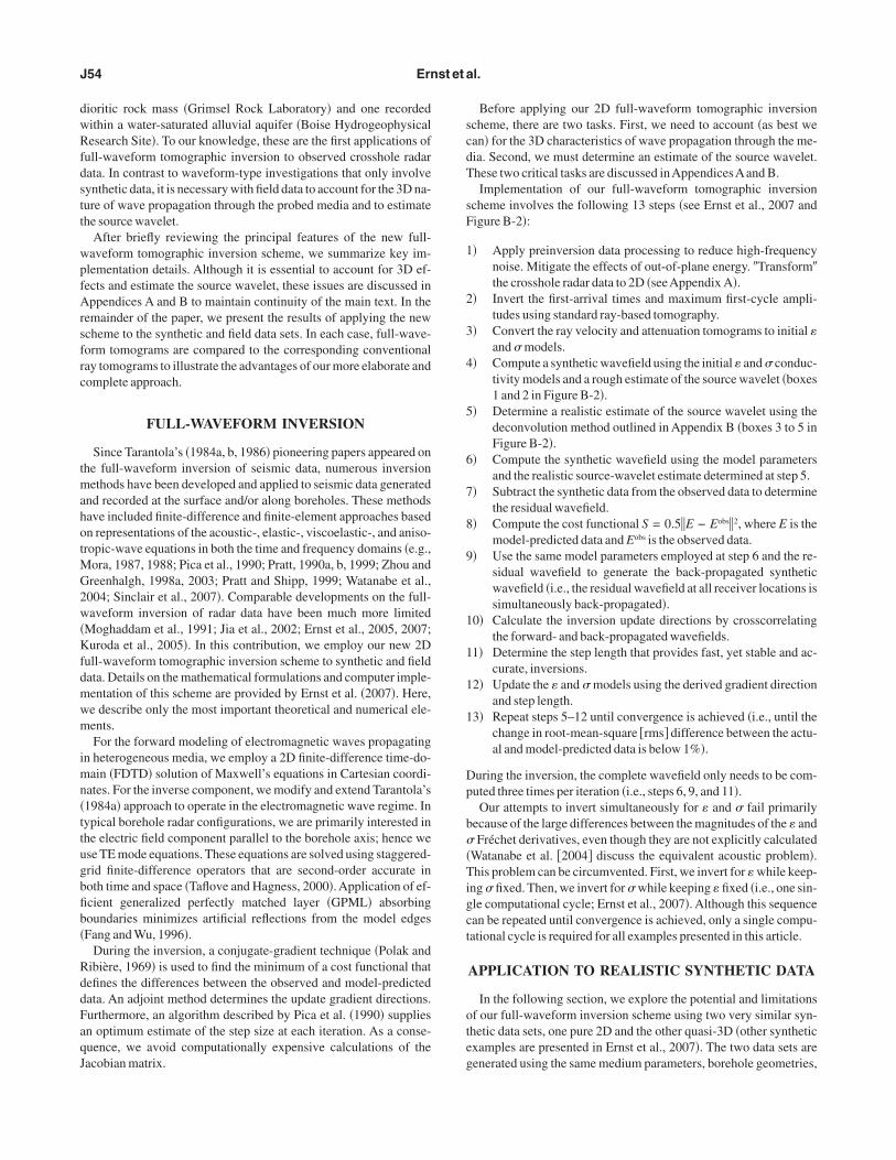
asis for an initial source-wavelet estimate that practically matcheshe true wavelet �compare the curves represented by the barely visi-le green and dashed black lines in Figure 2a; see also Appendix A�.sing the two ray tomograms and associated source-wavelet esti-ate as the initial input parameters, the full-waveform inversion

cheme for determining �r and the related source-wavelet computa-ions converge after 20 iterations. The subsequent full-waveform in-ersion scheme for � converges after 10 iterations.

ls were used for all ray-tomographic inversions.

ediumeters�mS/m��

Grid cell sizes�cm�

2.5D to 2Dtransformation/

sourceestimation andimprovement

Initialparameters

for raytomography��r and ��mS/m��Forward Inverse

; �mean = 1.4variationsd deviations, �std. = 1.7

tion lengths, z = 0.2 m

2 6 No / yes �r = 10.3� = 1.4

2 6 Yes / yes �r = 10.3� = 1.4

2 18 Yes / yes �r = 5.6� = 1.4

2 14 Yes / yes �r = 12.4� = 4.7

a) 0 2 4 6 8

10 12 14 16 18

12.0

11.5

11.0

10.5

10.0

9.5

9.0

8.5

8.0

Distance (m)

Dep

th (

m)

0 2 4 6 8 10

b) 0 2 4 6 8

10 12 14 16 18

Distance (m)

Dep

th (

m)

0 2 4 6 8 10

c) 0 2 4 6 8

10 12 14 16 18

Distance (m)

Dep

th (

m)

0 2 4 6 8 10

ε

d) 0 2 4 6 8

10 12 14 16 18

101

100

10–1

Distance (m)

Dep

th (

m)

0 2 4 6 8 10

e) 0 2 4 6 8

10 12 14 16 18

Distance (m)

Dep

th (

m)

0 2 4 6 8 10

f) 0 2 4 6 8

10 12 14 16 18

Distance (m)

Dep

th (

m)

0 2 4 6 8 10

σ (mS/m)

r

igure 1. �a� and �d� show input �r and � values for the 2D syntheticata experiment I �Table 1�. Mean dielectric permittivity and electri-al conductivity of the stochastic medium are �r

mean = 10.3 andmean = 1.4 mS/m. Standard deviations �r

std. = 0.8 and �std

1.7 mS/m. Correlation lengths in the x and z directions are 2 and.2 m; �b� and �e� show �r and � tomograms that result from apply-ng the ray-based inversion scheme to synthetic traces computedrom the model shown in �a� and �b�. Data were generated usingDTD approximations of Maxwell’s equation in 2D; �c� and �f� are

ike �b� and �e�, but for the full-waveform inversion. Black crossesnd circles indicate transmitter and receiver locations.

mode

nput mparamand �

= 10.3hastictandar

d. = 0.8orrela2.0 m

?

?

i�capWtrrsmme

mefowei

Swp

�

Fidwtpp

Fatti

J56 Ernst et al.

Because the source-wavelet estimate based on the ray tomogramss remarkably good, the full-waveform inversions do not improve itcompare the green, red, and dashed black lines in Figure 2a�. Byomparison, the full-waveform tomograms are significantly moreccurate with much higher resolution than the ray tomograms �com-are Figure 1c with a and b, and compare Figure 1f with d and e�.hereas the resolution of the ray tomograms is generally no better

han �1 m �i.e., the dominant wavelength of the radar signal�, theesolution of the full-waveform tomograms is in the 20–30 cmange. The full-waveform � tomogram accurately reconstructsmall-scale features in regions of the model that are well sampled byultiple crossing wavefronts. In contrast, the full-waveform � to-ogram predicts erroneously low � values at the upper and lower

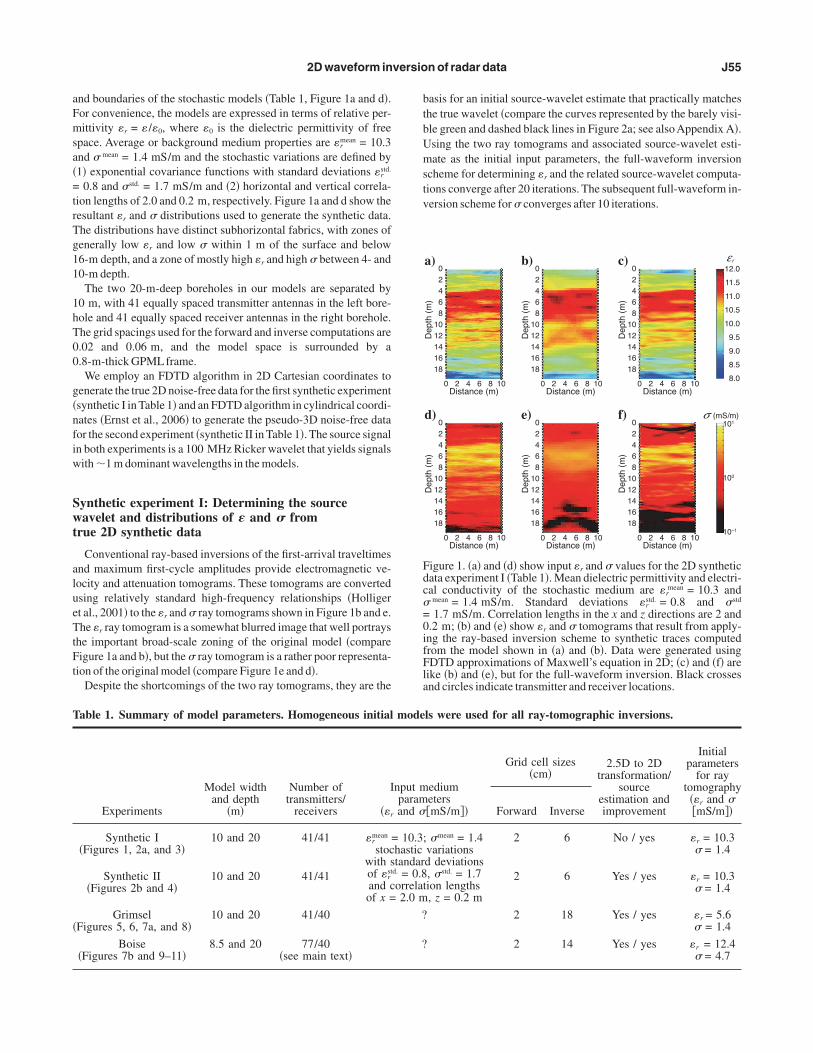
xtremities of the model �Figure 1f; seeAppendix B�.Figure 3 shows FDTD-generated receiver gathers for the originalodel and the ray and full-waveform tomograms. First-arrival trav-

ltimes and maximum first-cycle amplitudes of traces generatedrom the ray tomograms are quite close to those generated from theriginal model. However, small but important differences in theaveforms are exemplified in the difference plots of Figure 3c. Trac-

s generated from the full-waveform tomograms are practicallydentical to those generated from the original model.

ynthetic experiment II: Determining the sourceavelet and distributions of � and � fromseudo-3D synthetic data

We use the second synthetic data set created with Ernst et al.’s2006� FDTD code in cylindrical coordinates to demonstrate the ef-

s) t (ns)160 180

c)1

3

5

7

9

11

13

15

17

19

21

23

25

27

29

31

33

35

37

39

41

Trac

e nu

mbe

r

100 120 140 160 180

2x gain

ge at 10.1 m depth shown in Figure 1. Dashed black and solid bluet model in Figure 1a and d, the ray tomograms in Figure 1b and e, andw differences between the blue and dashed black lines in �a� and be-nd �b� are normalized with respect to the maximum amplitude of theative to the radar traces.

1.0

0.5

0

–0.5

–1.0

Time (ns)

Nor

mal

ized

am

plitu

de

0 5 10 15 20

a)

1.0

0.5

0

–0.5

–1.0

Time (ns)

Nor

mal

ized

am

plitu

de

0 5 10 15 20

b)

igure 2. �a and b� Source wavelets determined for the tomographicnversions that are shown in Figure 1 and Figure 4, respectively. Theashed black line shows the true source wavelet. Green and red lines,hich practically overlap, are the first and final source wavelets de-

ermined by the deconvolution method outlined inAppendix B.Am-litudes are normalized with respect to the maximum values for dis-lay purposes.

a)1

3

5

7

9

11

13

15

17

19

21

23

25

27

29

31

33

35

37

39

41

Trac

e nu

mbe

r

100 120 140t (ns) t (n

160 180

b)1

3

5

7

9

11

13

15

17

19

21

23

25

27

29

31

33

35

37

39

41

Trac

e nu

mbe

r

100 120 140

igure 3. �a and b� Transmitter gathers for a location along the left model ednd red lines show every second radar trace generated from the original inpuhe full-waveform tomograms in Figure 1c and f. �c� Blue and red lines shoween the red and dashed black lines in �b�, respectively.Amplitudes in �a� anput data.Amplitudes of residuals in �c� are amplified by a factor of two rel

figcrcdttFFegtmp

C

Lcmf1nst

wlat

D

o8��t2ss

Ds

rtce7a

Ffaaetsa

FfiT

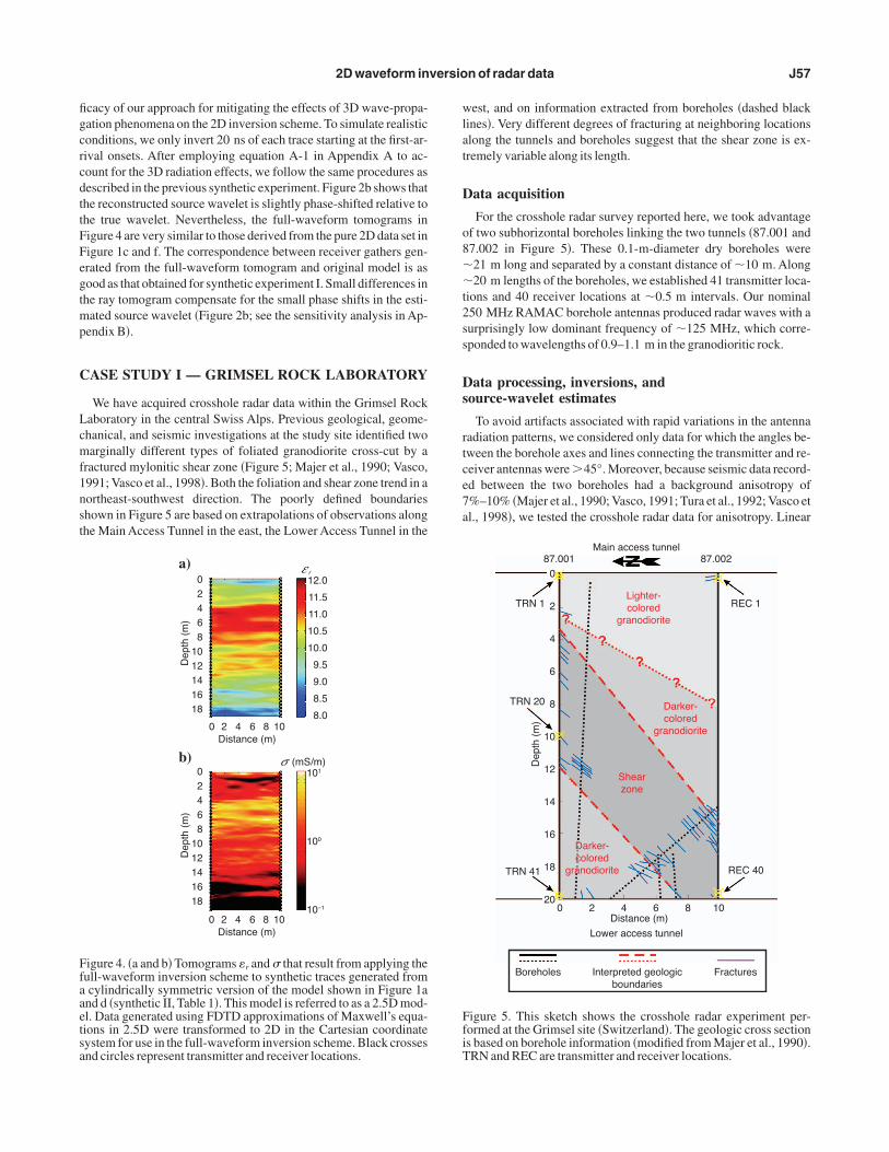
2D waveform inversion of radar data J57

cacy of our approach for mitigating the effects of 3D wave-propa-ation phenomena on the 2D inversion scheme. To simulate realisticonditions, we only invert 20 ns of each trace starting at the first-ar-ival onsets. After employing equation A-1 in Appendix A to ac-ount for the 3D radiation effects, we follow the same procedures asescribed in the previous synthetic experiment. Figure 2b shows thathe reconstructed source wavelet is slightly phase-shifted relative tohe true wavelet. Nevertheless, the full-waveform tomograms inigure 4 are very similar to those derived from the pure 2D data set inigure 1c and f. The correspondence between receiver gathers gen-rated from the full-waveform tomogram and original model is asood as that obtained for synthetic experiment I. Small differences inhe ray tomogram compensate for the small phase shifts in the esti-

ated source wavelet �Figure 2b; see the sensitivity analysis in Ap-endix B�.

ASE STUDY I — GRIMSEL ROCK LABORATORY

We have acquired crosshole radar data within the Grimsel Rockaboratory in the central Swiss Alps. Previous geological, geome-hanical, and seismic investigations at the study site identified twoarginally different types of foliated granodiorite cross-cut by a

ractured mylonitic shear zone �Figure 5; Majer et al., 1990; Vasco,991; Vasco et al., 1998�. Both the foliation and shear zone trend in aortheast-southwest direction. The poorly defined boundarieshown in Figure 5 are based on extrapolations of observations alonghe Main Access Tunnel in the east, the Lower Access Tunnel in the

12.0

11.5

11.0

10.5

10.0

9.5

9.0

8.5

8.0

02468

1012141618

Distance (m)

Dep

th (

m)

0 2 4 6 8 10

Distance (m)0 2 4 6 8 10

101

100

10–1

02468

1012141618

Dep

th (

m)

σ (mS/m)

a)

b)

ε r

igure 4. �a and b� Tomograms �r and � that result from applying theull-waveform inversion scheme to synthetic traces generated fromcylindrically symmetric version of the model shown in Figure 1a

nd d �synthetic II, Table 1�. This model is referred to as a 2.5D mod-l. Data generated using FDTD approximations of Maxwell’s equa-ions in 2.5D were transformed to 2D in the Cartesian coordinateystem for use in the full-waveform inversion scheme. Black crossesnd circles represent transmitter and receiver locations.

est, and on information extracted from boreholes �dashed blackines�. Very different degrees of fracturing at neighboring locationslong the tunnels and boreholes suggest that the shear zone is ex-remely variable along its length.

ata acquisition

For the crosshole radar survey reported here, we took advantagef two subhorizontal boreholes linking the two tunnels �87.001 and7.002 in Figure 5�. These 0.1-m-diameter dry boreholes were21 m long and separated by a constant distance of �10 m. Along20 m lengths of the boreholes, we established 41 transmitter loca-

ions and 40 receiver locations at �0.5 m intervals. Our nominal50 MHz RAMAC borehole antennas produced radar waves with aurprisingly low dominant frequency of �125 MHz, which corre-ponded to wavelengths of 0.9–1.1 m in the granodioritic rock.

ata processing, inversions, andource-wavelet estimates

To avoid artifacts associated with rapid variations in the antennaadiation patterns, we considered only data for which the angles be-ween the borehole axes and lines connecting the transmitter and re-eiver antennas were �45°. Moreover, because seismic data record-d between the two boreholes had a background anisotropy of%–10% �Majer et al., 1990; Vasco, 1991; Tura et al., 1992; Vasco etl., 1998�, we tested the crosshole radar data for anisotropy. Linear

0

2

4

6

8

10

12

14

16

18

20

Distance (m)

REC 40

REC 1TRN 1

TRN 20

TRN 41

Dep

th (

m)

0

87.001 87.002Main access tunnel

Lighter-colored

granodiorite

Darker-colored

granodiorite

Darker-colored

granodiorite

Shearzone

Lower access tunnel

Boreholes Interpreted geologicboundaries

Fractures

2 4 6 8 10

igure 5. This sketch shows the crosshole radar experiment per-ormed at the Grimsel site �Switzerland�. The geologic cross sections based on borehole information �modified from Majer et al., 1990�.RN and REC are transmitter and receiver locations.

ata�

imasd

tlvqc�Itg10ssamb

taTqacegi

gtMtmttf�

Cc

�br�ar

FicwaaF

Fstdaot

J58 Ernst et al.

nd polar plots of apparent velocity �i.e., transmitter-receiver dis-ance divided by first-arrival traveltime� versus transmitter-receiverngle �relative to the borehole axes� revealed negligible anisotropyi.e., �2.5%� in the radar data.

Figure 6a and c present ray tomograms that resulted from invert-ng the semiautomatically picked first-arrival traveltimes and maxi-

um first-cycle amplitudes. For the source-wavelet determinationnd the full-waveform inversion, we selected 42 ns of each tracetarting at the first-arrival onsets and then followed the same proce-ures as described for the synthetic data.

Whereas maximum cell sizes of forward-modeling grids are de-ermined by numerical stability criteria �Bergmann et al., 1996; Hol-iger and Bergmann, 2002�, there is no corresponding rule for the in-ersion cell sizes �Ernst et al., 2007�. There are two competing re-uirements to satisfy in defining the inversion cell sizes. �1� A suffi-ient number of grid points is needed to represent the radar signal.2� The number of grid points per antenna interval should be limited.f the number is not limited, then artifacts are generated near theransmitters and receivers as a result of their strong influence on theradient-computation component of the inversion process �i.e., step0 in the section, “Full-Waveform Inversion”�. Considering the.9–1.1 m radar wavelengths and the �0.5 m source and receiverpacing, a 0.18 m cell size is a reasonable compromise for the inver-ion of the Grimsel crosshole radar data.As for the synthetic data ex-mples, we use a conservative cell size of 0.02 m for the forwardodeling. The model space is surrounded by a 0.8-m-thick GPML

oundary.

7.0

6.5

6.0

5.5

5.0

4.5

a)02468

1012141618

Distance (m)

Dep

th (

m)

0

87.001 87.002 87.001 87.002

2 4 6 8 10

b)02468

1012141618

Distance (m)

Dep

th (

m)

0 2 4 6 8 10

ε

100

c)02468

1012141618

Distance (m)

Dep

th (

m)

0 2 4 6 8 10

d)02468

1012141618

Distance (m)

Dep

th (

m)

0 2 4 6 8 10

σ (mS/m)

r

igure 6. �a� and �c� show �r and � tomograms that result from apply-ng the ray-based tomographic inversion method to the Grimselrosshole radar traces. �b� and �d� are like �a� and �c�, but for the full-aveform inversion. Black crosses and circles represent transmitter

nd receiver locations. White lines portray the structural elements,nd black dashed lines indicate the additional boreholes shown inigure 5.

After 20 iterations for �r and 10 iterations for �, the full-waveformomograms of Figure 6b and d are obtained. Very similar tomogramsre obtained for inversion cell sizes ranging from 0.06 to 0.24 m.he small artifacts along the lengths of the boreholes are a conse-uence of the aforementioned high sensitivities near the transmittersnd receivers.Artifacts could be reduced by increasing the inversionell size, and thus distributing sensitivities over larger areas. Howev-r, this action would decrease the resolution in better sampled re-ions of the tomogram. The best way to eliminate these artifacts is toncrease the density of transmitter and receiver locations.

The source wavelets based on the ray and full-waveform tomo-rams are practically identical �Figure 7a�. The wavelets are charac-erized by two main cycles with a dominant frequency of �125

Hz. Despite these similarities and the close correspondence be-ween observed and ray-based first-arrival traveltimes and maxi-

um first-cycle amplitudes, there are important differences betweenhe observed and FDTD-generated radar traces derived from the rayomograms �Figure 8a and c�. In contrast, the radar traces generatedrom the full-waveform tomogram match closely the observed dataFigure 8b and c�.

omparison of radar and seismic P-wave velocityrosshole tomograms

Both �r tomograms in Figure 6 include regions of relatively highr values in the northwest and southeast separated by a prominentroad band of low �r values. This pattern is very similar to the patternevealed in the Grimsel P-wave velocity tomograms of Vasco1991�, Tura et al. �1992�, and Vasco et al. �1998�, except that moder-tely high seismic velocities in their tomograms coincide with lowadar velocities �i.e., high �r values� associated with the mostly in-

1.0

0.5

0

–0.5

–1.0

Time (ns)

Nor

mal

ized

am

plitu

de

0 5 10 15 20 25

a)

1.0

0.5

0

–0.5

–1.0

Time (ns)

Nor

mal

ized

am

plitu

de

0 5 10 15 20 25 30 35 40 45

b)

igure 7. �a� Source wavelets determined for the tomographic inver-ions shown in Figure 6 �Grimsel data set�. �b� Source wavelets de-ermined for the tomographic inversions shown in Figure 10 �Boiseata set�. Green and red lines, which practically overlap, are the firstnd final source wavelets determined by the deconvolution methodutlined in Appendix B. Amplitudes are normalized with respect tohe maximum values for display purposes.

tv

I

fmsvcttaurs

aeit�ns

w

w�l

ddi�bsa2

D

bardDt0a

Fs�p

2D waveform inversion of radar data J59

act rock mass and low seismic velocities coincide with high radarelocities �i.e., low �r values� associated with the shear zone.

nterpretation

As for the synthetic data examples, the resolution of the Grimselull-wave radar tomograms is markedly superior to that of the ray to-ograms; smaller features are imaged and the �r and � contrasts are

tronger and sharper. In both suites of tomograms, a pattern of low �r

alues follows the northeast-southwest trend of the shear zone. Ac-ording to the full-wave tomograms, its northwest boundary is dis-inguished by relatively abrupt changes from �r �4.75–5.75 withinhe shear zone to �r �5.75–6.50 outside. If relatively low �r valuesre caused by fracturing, then the full-waveform �r tomogram �Fig-re 6b� suggests that the southeast boundary of the shear zone is alsoelatively abrupt and occurs �4 m further to the southeast thanhown in Figure 5.

Although � changes from generally less than 1.5 mS/m to mostlybove 2.5 mS/m across the northwest boundary of the shear zone,vidence for the shear zone is less obvious in the � tomograms thann the �r tomograms. Because � is controlled by the highest conduc-ivity component of a system, the presence of relatively dry fractureswhich do not interrupt current flow through the matrix� does not sig-ificantly influence the average conductivity distribution in the con-idered area.

The evidence from the radar and seismic tomograms is consistentith the presence of fractures interpreted from borehole log data

a)1

3

5

7

9

11

13

15

17

19

21

23

25

27

29

31

33

35

37

39

Trac

e nu

mbe

r

1

3

5

7

9

11

13

15

17

19

21

23

25

27

29

31

33

35

37

39

Trac

e nu

mbe

r

80 100 120t (ns)

140 80

b)

igure 8. �a and b� Transmitter gathers for location TRN 20 in Figurerved radar trace and data generated from the ray tomograms in Figuc� Blue and red lines show the differences between the blue and dashlitudes in all panels are normalized with respect to the maximum am

ithin the cross-cutting shear zone. These fractures are likely filledor partially filled� with air or other low �r, low to moderate �, andow P-wave velocity material.

CASE STUDY II — BOISE HYDROGEOPHYSICALRESEARCH SITE

Our second crosshole radar data set was collected at the Boise Hy-rogeophysical Research Site in Idaho �Tronicke et al., 2004�. Aense array of boreholes at this site has been used for diverse geolog-c, geomechanical, hydrogeological, and geophysical experimentsClement et al., 1999; Barrash and Clemo, 2002; Barrash and Re-oulet, 2004; Tronicke et al., 2004; Clement and Barrash, 2006�. Theite has an approximately 20-m-thick deposit of braided-river gravelnd sand, and an underlying clay layer. The water table was at.96 m depth at the time of the measurements.

ata acquisition

Tronicke et al.’s �2004� data were acquired in two 0.1-m-diameteroreholes that were �20 m deep and separated by �8.5 m �see C6nd C5 in Figure 9�. The boreholes, which were slightly tilted withespect to the vertical, penetrated three distinct pebble- and cobble-ominated layers with 21%, 26%, and 26% porosities �Figure 9�.ata acquisition extended from �4 to �19.4 m in depth, with 77

ransmitter locations at 0.2 m intervals, and 40 receiver locations at.4 m intervals. Although the nominal 250 MHz RAMAC boreholentennas produced even lower frequencies than at Grimsel because

1

3

5

7

9

11

13

15

17

19

21

23

25

27

29

31

33

35

37

39

Trac

e nu

mbe

r

120(ns)

140 80 100 120

t (ns)140

c)

e dashed black and solid blue and red lines show every second ob-nd c, and full-waveform tomograms in Figure 6b and d, respectively.ck lines in �a� and between the red and dashed black lines in �b�.Am-

of the input data.

100t

e 5. Thre 6a aed blaplitude

owi

Ds

atwtmfias

FtamasE

ac

tcqa

I

obtttibswttsr

chftcv

FB�l

a

c

Ftrsaccs

J60 Ernst et al.

f the water-saturated environment, the dominant �80 MHz radaraves had similar 0.9–1.1 m wavelengths in the high-�r �low veloc-

ty� sediments.

ata processing, inversions, andource-wavelet estimates

The data processing, inversions, and wavelet estimate procedurespplied to the Boise data set were very similar to those described forhe synthetic and Grimsel data sets. We considered only data forhich the angles between the borehole axes and lines connecting the

ransmitter and receiver antennas were �45°.Anisotropy was deter-ined to be negligible �i.e., �2%�. We used 78 ns of data after therst-arrival onsets in the waveform inversion. Forward modelingnd inverse grid cell sizes were 0.02 and 0.14 m, and the modelpace was surrounded by a 0.8-m-thick GPML boundary.

The resultant ray tomograms are displayed in Figure 10a and c.igure 10b and d show the full-waveform tomograms after 30 itera-

ions for �r and 8 iterations for �. Like the synthetic and Grimsel ex-mples, the source wavelets based on the ray and full-waveform to-ograms are practically identical �Figure 7b�. The reverberant char-

cter of the relatively long source wavelet may be a result of the Boi-e boreholes being filled with water �Holliger and Bergmann, 2002;rnst et al., 2006�.There are notable misfits between the observed and FDTD-gener-

ted radar traces derived from the ray tomograms, particularly in theentral regions of the receiver gather of Figure 11a and c. The radar

0

2

4

6

8

10

12

14

16

18

Distance (m)

REC 1

TRN 1

TRN 20

TRN 40 REC 77

Dep

th (

m)

0

C5 C6

Surface

Water table

Pebble- and cobble-dominated braided river

deposits by porosity:

21%

26%

23%

Boreholes Interpreted geologic boundaries

2 4 6 8

?

igure 9. Sketch of the crosshole radar experiment performed at theoise site �Idaho�. Geologic boundaries are based on porosity logs

Tronicke et al., 2004�. TRN and REC are transmitter and receiverocations.

races generated from the full-waveform tomogram correspondlosely to the observed ones in Figure 11b and c, but the match is notuite as good as for the synthetic and Grimsel examples �Figures 3nd 8�.

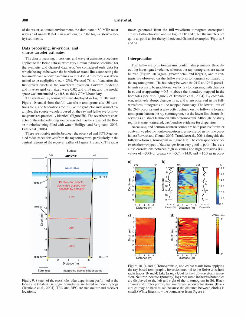
nterpretation

The full-waveform tomograms contain sharp images through-ut the investigated volume, whereas the ray tomograms are ratherlurred �Figure 10�. Again, greater detail and larger �r and � con-rasts are observed on the full-waveform tomograms compared tohe ray tomograms. The boundary between the 21% and 26% porosi-y units seems to be gradational on the ray tomograms, with changesn �r and � appearing �0.5 m above the boundary mapped in theoreholes �see also Figure 7 of Tronicke et al., 2004�. By compari-on, relatively abrupt changes in �r and � are observed in the full-aveform tomograms at the mapped boundary. The lower limit of

he 26% porosity unit is also better defined on the full-waveform �r

omogram than on the ray �r tomogram, but the lower limit is not ob-erved as a distinct feature on either � tomogram.Although the studyegion is water-saturated, we found no evidence for dispersion.

Because �r and neutron-neutron counts are both proxies for waterontent, we plot the neutron-neutron logs measured in the two bore-oles �Barrash and Clemo, 2002; Tronicke et al., 2004� alongside theull-waveform �r tomogram in Figure 10b. The correspondence be-ween the two types of data ranges from very good to poor. There arelose correlations between high �r values and high porosities �i.e.,alues of �30% or greater� at �5.7, �14.8, and �16.5 m in bore-

16.0

15.0

14.0

13.0

12.0

11.0

10.0

) 4

6

8

10

12

14

16

18

Distance (m)

Dep

th (

m)

0

C5 C6

2 4 6 8Distance (m)

4

6

8

10

12

14

16

18

Dep

th (

m)

0

C5 C6

2 4Porosity (%)

30 10 50 Porosity (%)

30 10 50 6 8

4

6

8

10

12

14

16

18

Distance (m)

Dep

th (

m)

0 2 4 6 8

4

6

8

10

12

14

16

18

Distance (m)

Dep

th (

m)

0 2 4 6 8

b) ε

101

100

) d) σ (mS/m)

r

igure 10. �a and c� Tomograms �r and � that result from applyinghe ray-based tomographic inversion method to the Boise crossholeadar traces. �b and d� Like �a and c�, but for the full-waveform inver-ion. Neutron-neutron �porosity� logs measured in the two boreholesre displayed to the left and right of the �r tomogram in �b�. Blackrosses and circles portray transmitter and receiver locations. �Blackircles may be hard to see because the distance between circles ismall.� White lines show the boundaries from Figure 9.

hsetn�z

mcsptmmgfw

w

sdtwths

3rcdts

aiep

Soq

FrTp

2D waveform inversion of radar data J61

ole C5, and at �6.1, �11.3, and �14.8 m in borehole C6. There areeveral moderately high porosity values in the two logs that have noxpression in the tomogram. The zone of high �r values that spanshe tomogram at �12.5 m depth has no expression in either neutron-eutron log. We note, however, that the zone of high �r values at12.5-m depth thins as it approaches both boreholes, such that the

one may not be apparent in the porosity measurements.

CONCLUSIONS

We outline the essential elements of a new 2D full-waveform to-ographic inversion scheme and describe simple methods to ac-

ount for 3D radar-wave propagation effects and to estimate theource wavelet. We apply the new scheme to realistic pure 2D andseudo-3D synthetic data, as well as to field data acquired in rela-ively dry crystalline rock and water-saturated unconsolidated sedi-

ents. In all four examples, the resolution of the full-waveform to-ograms is significantly superior to that of the respective ray tomo-

rams. Boundaries between structural units are sharply focused, andeatures with dimensions as small as 0.3–0.5 of the dominant radaravelength are clearly imaged in the full-waveform tomograms.Although transmitter and receiver intervals of half the dominant

avelength prove to be suitable for the synthetic case studies, the re-

a)1

4

7

10

13

16

19

22

25

28

31

34

37

40

43

46

49

52

55

58

61

64

67

70

73

76

Trac

e nu

mbe

r

Trac

e nu

mbe

r

100 120 140t (ns)

160

1

4

7

10

13

16

19

22

25

28

31

34

37

40

43

46

49

52

55

58

61

64

67

70

73

76

100 12

b)

igure 11. �a and b� are receiver gathers for location REC 20 in Figureadar trace and data generated from the ray tomograms in Figure 10ahe blue and red lines that show differences between the blue and daslitudes in all panels are normalized with respect to the maximum am

ults of inverting the field data suggest that the intervals should be re-uced to approximately half this value to avoid artifacts near the an-ennas. In an investigation of potential trade-offs between source-avelet estimates and the full-waveform tomograms, we find that al-

hough realistic timing errors in the source wavelets are unlikely toave major effects on � tomograms, small amplitude errors may re-ult in moderately inaccurate � tomograms.

The ray-based inversions required about 0.5 hours on a single2-bit Intel Xeon 2.4 GHz processor. The full-waveform inversionsequired less than 12 hours on N + 1 64-bit AMD 244 1.8 GHz pro-essors �where N is the number of transmitters�. Clearly, users mustecide whether the significant improvement in resolution is worthhe extra computational effort required for the full-waveform inver-ions.

Considering that the source wavelet may vary along the length ofborehole according to local conditions, future developments may

nclude the possibility of determining and using a source wavelet forach transmitting regime of a borehole to account for different cou-lings and near-borehole heterogeneities.

ACKNOWLEDGMENTS

This research was supported by grants from ETH Zurich and thewiss National Science Foundation. We thank NAGRA �Swiss Co-perative for the Storage of Nuclear Waste� for cooperation in ac-uiring the Grimsel crosshole data set. Thanks are due to Roland

Trac

e nu

mbe

r

140 160

1

4

7

10

13

16

19

22

25

28

31

34

37

40

43

46

49

52

55

58

61

64

67

70

73

76

100 120 140t (ns)

160

c)

dashed black and solid blue and red lines show every third observedand full-waveform tomograms in Figure 10b and d, respectively. �c�ck lines in �a� and between the red and dashed black lines in �b�.Am-of the input data.

0t (ns)

9. Theand c

hed blaplitude

GiTcomp

peciehfchwcdv

pesw�dtpb1thIs�o

Itmcmnotd

F

yst1

wvrsJwpa1tsep

D

lmtglptbe

F�lgsFmta

J62 Ernst et al.

ritto, Peter Schuler, and Peter Blümling for supplying importantnformation associated with the Grimsel test site. We also thank Jensronicke, Warran Barrash, and Bill Clement for providing the Boiserosshole data set and relevant information. Further, Bernard Gir-ux, Stewart Greenhalgh, and Lars Nielsen provided helpful com-ents and suggestions on an earlier draft of this paper. ETH-Geo-

hysics Publication no. 1494.

APPENDIX A

ACCOUNTING FOR 3D EFFECTS

Crosshole radar data are invariably influenced by 3-D wave-ropagation phenomena, including both out-of-plane and radiationffects. Because most crosshole radar data are acquired with single-omponent nondirectional antennas, there is generally insufficientnformation to discriminate between out-of-plane and in-planevents. Nevertheless, for media characterized by moderate velocityeterogeneity, the vast majority of energy contributing to the firstew cycles of a recorded trace likely originates from within the planeontaining the transmitter and receiver antennas. For typical cross-ole experiments, the initial pulse can contain only energy fromithin a wavelength or two of this plane. Consequently, to minimize

ontamination from out-of-plane energy, we consider only time win-ows that include the first few cycles of the recorded traces in the in-ersion �see discussions by Pratt, 1999 and Pratt and Shipp, 1999�.

In applying 2D computational codes in many disciplines of geo-hysics, sources and structures are assumed to extend to infinity onither side of the observation plane. In our FDTD algorithm, theources are effectively modeled as infinite lines of point dipoles.Yet,e know that real antennas radiate energy in three dimensions.

Ernst et al. �2006� have shown that the radiation pattern of a pointipole closely approximates that of the common insulated Wu-King-ype antenna.� An algorithm that explicitly incorporates 3D waveropagation in a medium that varies in only two dimensions woulde one way of addressing this issue �e.g., Zhou and Greenhalgh,998b�. Unfortunately, implementation of such an approach in ourime-domain scheme would be very computationally costly. Weave chosen an alternative approach proposed by Bleistein �1986�.n this approach, appropriate corrections are made for 3D geometricpreading, a �/4 phase shift, and a frequency scaling effect of 1/��where � is the angular frequency�. The corrections are made to thebserved data in the frequency domain as follows:

E2D�xtrn,xrec,�� = Eobs�xtrn,xrec,���2�T�xtrn,xrec�− i��mean�

,

�A-1�

n equation A-1, E2D�xtrn,xrec,�� is the corrected data for a transmit-er at location xtrn�x,z� and a receiver at xrec�x,z�. A frequency-do-

ain parameter is indicated by ˆ. Eobs�xtrn,xrec,�� is the original re-orded data; T�xtrn,xrec� is the traveltime; i2 = − 1; and �mean is theean dielectric permittivity of the media. We set � = �0, the mag-

etic permeability of free space. Thorough testing of this approachn synthetic crosshole radar data demonstrates good agreement be-ween corrected 3D and corresponding pure 2D data, as long as theata are generated for far-field regimes.

APPENDIX B

SOURCE WAVELET ESTIMATION

irst-arrival pulse method

Our first attempt to determine the source wavelet is based on anal-ses of the first-arrival pulses. The following relationship links theource current density Jtrn that we employ in our FDTD algorithm tohe recorded electric field in the far-field regime Eobs �de Hoop,995�:

Jtrn�xtrn,t� � t�

Eobs�xrec,t��dt�, �B-1�

here t is time. We avoid problems associated with radiation-angleariations by considering only data from shortest-path transmitter-eceiver pairs �i.e., those with radiation angles�90°�. To obtain aingle estimate of the source wavelet �i.e., in terms of current density� and to minimize the influence of near-borehole heterogeneities,e integrate the radar data according to equation B-1 and then com-ute the average of the extracted first-arrival pulses. An example ofpplying this procedure to synthetic data set I �Figures 1–3 and Table� is shown by the blue curve in Figure B-1. Although the shape ofhis source-wavelet estimate is generally similar to that of the trueource wavelet �black dashed line in Figure B-1�, it is not closenough; the resultant tomograms are unsatisfactory. This methoderforms poorly on all synthetic and observed data sets.

econvolution method

The key steps of our second attempt to determine the source wave-et are outlined in Figure B-2. Our radar data can be represented

athematically as the convolution of the true source wavelet withhe true impulse response �i.e., suite of spike radargrams� of the re-ion of earth under investigation. In principle, the true source wave-et can be obtained by deconvolving the radar data with the true im-ulse response of the earth. Of course, we do not know the latter. For-unately, very good estimates of the source wavelet can be obtainedy deconvolving the recorded data with our best estimates of thearth’s impulse response.

1.0

0.5

0

–0.5

–1.0

Time (ns)

Nor

mal

ized

am

plitu

de

0

± 1 ns

5 10 15 20

30%

1 ns+–

igure B-1. Source wavelet reconstructions for the 2D synthetic dataFigure 1�. The dashed black line is the true source wavelet, the blueine is the source wavelet based on the first-pulse method, and thereen and red lines, which practically overlap, are the first and finalource wavelets based on the deconvolution method outlined inigure B-2. Amplitudes are normalized with respect to the maxi-um values for display purposes. The ± 1 ns and 30% bars indicate

he phase shifts and amplitude variations used in the sensitivitynalyses.

mgswcsasetswddemcEt

talcgS�wtt2

Si

stipdBtFtttns

B

B

B

B

B

C

C

C

C

C

C

—Fe

2D waveform inversion of radar data J63

At the beginning of the full-waveform inversion, our best esti-ates of the � and � distributions are provided by the ray tomo-

rams. It is not possible to compute directly the earth’s impulse re-ponse using our FDTD code, because an infinitesimal grid spacingould be required for computations involving a spike source. To cir-

umvent this problem, we first employ the FDTD code to compute auite of synthetic radargrams Esyn��k=0,�k=0,Sk=0�t�,t� using the �ray

nd �ray distributions defined by the ray tomograms and a plausibleource wavelet Sk=0�t� �boxes 1 and 2 in Figure B-2�, where k is the it-ration number. We use the source wavelet Sini�t� determined fromhe analysis of the first-arrival pulses for this purpose; however, anyource wavelet with comparable length and frequency contentould be sufficient at this stage. After Fourier transformation, weeconvolve �i.e., division in the frequency domain� the syntheticata Esyn�f� with Sk=0�f� to give a frequency-domain estimate of thearth’s impulse response M�f�, where ˆ indicates a frequency-do-ain parameter and f is frequency �box 3 in Figure B-2�. Finally, de-

onvolution of the frequency-domain version of the observed dataˆ obs�f� with M�f� and inverse Fourier transformation provides an es-imate of the source wavelet Sk=1�t� �boxes 4 and 5 in Figure B-2�.

Initialforward modeling

k =

k+

1

Waveform Inversionsteps 6-13 in main text No Yes

NoYesEnd

Source waveletrefinement required?

Convergence instep 6?

E: Electric fieldM: Impulse response of modelS: Source wavelet : Permittivity : Conductivity

ObservationSyntheticRay-inversionInitialIteration numberFrequency domain

obs:syn:ray:ini:k:^:

(1)

Esyn( k, k, Sk(t), t)

FFT {Sk(t)}, FFT {Esyn(t )}

FFT {E obs(t)}

IFFT {Sk+1(f )}

(2)

M(f ) = E syn(f ) [Sk(f )]–1(3) ^ ^ ^

Sk+1(f ) = [M(f )]–1 E obs(f )(4)

Sk+1(t)(5)

(6)

(7)

(8)

^ ^ ^

^

Sk=0(t) = Sini(t); k=0 = ray; k=0 = ray

k=0 = ray

k+1 & k+1

k=0 = ray

εσ

σ

σ σ

ε

σ σε ε

ε

σε

ε

igure B-2. Aflow chart outlining the deconvolution source-waveletstimation method. �See text for details.�

Because the equation in box 4 of Figure B-2 describes an over-de-ermined problem, in which far more data than unknowns are avail-ble, we estimate Sk=1�f� by fitting the observations in a minimumeast-squares sense. Although the process represented by steps 2–5an be repeated using progressively improved full-waveform tomo-rams �e.g., after every tenth iteration, see box 7 in Figure B-2�,

ˆk=1�f� already matches closely the true source wavelet in Figure B-1compare the solid green and dashed black lines�. Indeed, sourceavelets based on the ray tomograms are uniformly very close to

hose based on the best full-waveform tomograms for all of our syn-hetic and field data sets �compare the green and red lines in Figures, 7, and B-1�.

ensitivity of the tomograms to errorsn the source wavelet

The potential exists for trade-offs between the properties of theource wavelet and those of the tomograms. We test the effects ofhese trade-offs using the source wavelet of synthetic data set I. Wentroduce ±1 ns phase shifts to the source wavelet �the form and am-litude of the wavelet are not changed�, which correspond to �10ata samples and would be very visible in the radargrams �Figure-1�. This introduction results in rms differences of �2.3% between

he final full-waveform � tomogram and the original input model.or no phase shift, the rms difference is 1.6%. Artificially reducing

he amplitude of the source wavelet by �30% �the form and phase ofhe wavelet are not changed� results in a 13% rms difference betweenhe logarithm of the final full-waveform � tomogram and the origi-al input model �whereas the rms difference is only 5% for the trueource wavelet�.

REFERENCES

arrash, W., and T. Clemo, 2002, Hierarchical geostatistics and multi-facies systems: Boise Hydrogeophysical Research Site, Boise, Idaho:Water Resources Research, 38, 1196; http://dx.doi.org/1110.1029/2002WR001436.

arrash, W., and E. C. Reboulet, 2004, Significance of porosity for stratigra-phy and textural composition in subsurface, coarse fluvial deposits: BoiseHydrogeophysical Research Site: Geological Society ofAmerica Bulletin,116, 1059–1073.

ellefleur, G., and M. Chouteau, 2001, Massive sulphide delineation usingborehole radar: Tests at the McConnell nickel deposit, Sudbury, Ontario:Journal ofApplied Geophysics, 47, 45–61.

ergmann, T., J. O.A. Robertsson, and K. Holliger, 1996, Numerical proper-ties of staggered finite-difference solutions of Maxwell’s equations forground-penetrating radar modeling: Geophysical Research Letters, 23,45–48.

leistein, N., 1986, 2-1/2 dimensional inplane wave-propagation: Geophys-ical Prospecting, 34, 686–703.

ai, W. Y., F. H. Qin, and G. T. Schuster, 1996, Electromagnetic velocity in-version using 2-D Maxwell’s equations: Geophysics, 61, 1007–1021.

arlsten, S., S. Johansson, and A. Worman, 1995, Radar techniques for indi-cating internal erosion in embankment dams: Journal ofApplied Geophys-ics, 33, 143–156.

hew, W. C., and Y. M. Wang, 1990, Reconstruction of 2-dimensional per-mittivity distribution using the distorted Born iterative method: IEEETransactions on Medical Imaging, 9, 218–225.

lement, W. P., and W. Barrash, 2006, Crosshole radar tomography in a fluvi-al aquifer near Boise, Idaho: Journal of Environmental and EngineeringGeophysics, 11, 171–184.

lement, W. P., M. D. Knoll, L. M. Liberty, P. R. Donaldson, P. Michaels, W.Barrash, and J. R. Pelton, 1999, Geophysical surveys across the Boise Hy-drogeophysical Research Site to determine geophysical parameters of ashallow, alluvial aquifer: Proceedings, Symposium on the Application ofGeophysics to Engineering and Environmental Problems, 399–408.

ui, T. J., and W. C. Chew, 2000, Novel diffraction tomographic algorithmfor imaging two-dimensional targets buried under a lossy earth: IEEETransactions on Geoscience and Remote Sensing, 38, 2033–2041.—–, 2002, Diffraction tomographic algorithm for the detection of three-di-

C

C

d

E

—

E

F

F

H

H

I

J

J

K

M

M

—

M

M

—

M

O

P

P

P

P

—

—

P

S

S

T

T

—

—

T

T

T

V

V

W

W

W

Z

—

—

Z

J64 Ernst et al.

mensional objects buried in a lossy half-space: IEEE Transactions on An-tennas and Propagation, 50, 42–49.

ui, T. J., W. C. Chew, A. A. Aydiner, and S. Y. Chen, 2001, Inverse scatter-ing of two-dimensional dielectric objects buried in a lossy earth using thedistorted Born iterative method: IEEE Transactions on Geoscience andRemote Sensing, 39, 339–346.

ui, T. J., Y. Qin, G. Y. Wang, and W. C. Chew, 2004, Low-frequency detec-tion of two-dimensional buried objects using high-order extended Bornapproximations: Inverse Problems, 20, S41–S62.

e Hoop, A. T., 1995, Handbook of radiation and scattering of waves:Acous-tic waves in fluids, elastic waves in solids, electromagnetic waves: Aca-demic Press.

rnst, J. R., K. Holliger, H. Maurer, and A. G. Green, 2005, Full-waveforminversion of crosshole georadar data: 75th Annual International Meeting,SEG, ExpandedAbstracts, 2573–2577.—–, 2006, Realistic FDTD modelling of borehole georadar antenna radia-tion: Methodology and application: Near Surface Geophysics, 4, 19–30.

rnst, J. R., H. Maurer, A. G. Green, and K. Holliger, 2007, Full-waveforminversion of crosshole radar data based on 2-D finite-difference time-do-main �FDTD� solutions of Maxwell’s equations: IEEE Transactions onGeoscience and Remote Sensing.

ang, J. Y., and Z. H. Wu, 1996, Generalized perfectly matched layer for theabsorption of propagating and evanescent waves in lossless and lossy me-dia: IEEE Transactions on Microwave Theory and Techniques, 44,2216–2222.

ullagar, P. K., D. W. Livelybrooks, P. Zhang, A. J. Calvert, and Y. R. Wu,2000, Radio tomography and borehole radar delineation of the McConnellnickel sulfide deposit, Sudbury, Ontario, Canada: Geophysics, 65,1920–1930.

olliger, K., and T. Bergmann, 2002, Numerical modeling of borehole geo-radar data: Geophysics, 67, 1249–1257.

olliger, K., M. Musil, and H. R. Maurer, 2001, Ray-based amplitude to-mography for crosshole georadar data:Anumerical assessment: Journal ofApplied Geophysics, 47, 285–298.

rving, J. D., and R. J. Knight, 2005, Effect of antennas on velocity estimatesobtained from crosshole GPR data: Geophysics, 70, no. 5, K39–K42.

ia, H. T., T. Takenaka, and T. Tanaka, 2002, Time-domain inverse scatteringmethod for cross-borehole radar imaging: IEEE Transactions on Geo-science and Remote Sensing, 40, 1640–1647.

ohnson, T. C., P. S. Routh, and M. D. Knoll, 2005, Fresnel volume georadarattenuation-difference tomography: Geophysical Journal International,162, 9–24.

uroda, S., M. Takeuchi, and H. J. Kim, 2005, Full waveform inversion algo-rithm for interpreting cross-borehole GPR data: 75th Annual InternationalMeeting, SEG, ExpandedAbstracts, 1176–1180.ajer, E. L., L. R. Myer, J. E. Peterson, K. Karasaki, J. C. S. Long, S. J. Mar-tel, P. Blümling, and S. Vomvoris, 1990, Joint seismic, hydrogeological,and geomechanical investigations of a fractured zone in the Grimsel RockLaboratory, Switzerland: NAGRA-DOE Cooperative Project Report.oghaddam, M., and W. C. Chew, 1992, Nonlinear 2-dimensional velocityprofile inversion using time domain data: IEEE Transactions on Geo-science and Remote Sensing, 30, 147–156.—–, 1993, Study of some practical issues in inversion with the Born itera-tive method using time-domain data: IEEE Transactions on Antennas andPropagation, 41, 177–184.oghaddam, M., W. C. Chew, and M. Oristaglio, 1991, Comparison of theBorn iterative method and Tarantola’s method for an electromagnetictime-domain inverse problem: International Journal of Imaging Systemsand Technology, 3, 318–333.ora, P., 1987, Nonlinear two-dimensional elastic inversion of multioffsetseismic data: Geophysics, 52, 1211–1228.—–, 1988, Elastic wave-field inversion of reflection and transmission data:Geophysics, 53, 750–759.usil, M., H. Maurer, K. Hollinger, and A. G. Green, 2006, Internal structureof an alpine rock glacier based on crosshole georadar traveltimes and am-plitudes: Geophysical Prospecting, 54, 273–285.

lsson, O., L. Falk, O. Forslund, L. Lundmark, and E. Sandberg, 1992, Bore-hole radar applied to the characterization of hydraulically conductive frac-ture-zones in crystalline rock: Geophysical Prospecting, 40, 109–142.

aasche, H., J. Tronicke, K. Holliger, A. G. Green, and H. Maurer, 2006, In-

tegration of diverse physical-property models: Subsurface zonation andpetrophysical parameter estimation based on fuzzy c-means cluster analy-ses: Geophysics, 71, no. 3, H33–H44.

ica, A., J. P. Diet, and A. Tarantola, 1990, Nonlinear inversion of seismic-re-flection data in a laterally invariant medium: Geophysics, 55, 284–292.

olak, E., and G. Ribière, 1969, Note on convergence of conjugate directionmethods: Revue Française d’Informatique de Recherche Opérationnelle,3, 35–43.

ratt, R. G., 1990a, Frequency-domain elastic wave modeling by finite-dif-ferences—A tool for crosshole seismic imaging: Geophysics, 55,626–632.—–, 1990b, Inverse-theory applied to multisource cross-hole tomography.Part 2: Elastic wave-equation method: Geophysical Prospecting, 38,311–329.—–, 1999, Seismic waveform inversion in the frequency domain, Part 1:Theory and verification in a physical scale model: Geophysics, 64,888–901.

ratt, R. G., and R. M. Shipp, 1999, Seismic waveform inversion in the fre-quency domain, Part 2: Fault delineation in sediments using crossholedata: Geophysics, 64, 902–914.

ena, A. G., and M. N. Toksoz, 1990, Simultaneous reconstruction of permit-tivity and conductivity for crosshole geometries: Geophysics, 55,1302–1311.

inclair, C., S. A. Greenhalgh, and B. Zhou, 2007, 2.5-D modelling of elasticwaves in anisotropic media using the spectral element method—Aprelim-inary investigation: Exploration Geophysics.

aflove, A., and S. C. Hagness, 2000, Computational electrodynamics, the fi-nite-difference time-domain method:Artech House.

arantola, A., 1984a, Inversion of seismic-reflection data in the acoustic ap-proximation: Geophysics, 49, 1259–1266.—–, 1984b, The seismic reflection inverse problem, in F. Santosa, Y.-H.Pao, W. Symes, and C. Holland, eds., Inverse problems of acoustic andelastic waves: SIAM.—–, 1986, A strategy for nonlinear elastic inversion of seismic-reflectiondata: Geophysics, 51, 1893–1903.

ronicke, J., K. Holliger, W. Barrash, and M. D. Knoll, 2004, Multivariateanalysis of cross-hole georadar velocity and attenuation tomograms foraquifer zonation: Water Resources Research, 40, W01519; http://dx-.doi.org/10.1029/2003WR002031.

ronicke, J., D. R. Tweeton, P. Dietrich, and E. Appel, 2001, Improved cross-hole radar tomography by using direct and reflected arrival times: JournalofApplied Geophysics, 47, 97–105.

ura, M. A. C., L. R. Johnson, E. L. Majer, and J. E. Peterson, 1992, Applica-tion of diffraction tomography to fracture detection: Geophysics, 57, 245–257.

asco, D. W., 1991, Bounding seismic velocities using a tomographic meth-od: Geophysics, 56, 472–482.

asco, D. W., J. E. Peterson, and E. L. Majer, 1998, Resolving seismic aniso-tropy: Sparse matrix methods for geophysical inverse problems: Geophys-ics, 63, 970–983.ang, Y. M., and W. C. Chew, 1989, An iterative solution of the two-dimen-sional electromagnetic inverse scattering problem: International Journalof Imaging Systems and Technology, 1, 100–108.atanabe, T., K. T. Nihei, S. Nakagawa, and L. R. Myer, 2004, Viscoacousticwaveform inversion of transmission data for velocity and attenuation:Journal of theAcoustical Society ofAmerica, 115, 3059–3067.illiamson, P. R., and M. H. Worthington, 1993, Resolution limits in ray to-mography due to wave behavior—Numerical experiments: Geophysics,58, 727–735.

hou, B., and S. A. Greenhalgh, 1998a, Crosshole acoustic velocity imagingwith the full-waveform spectral data: 2.5-D numerical simulations: Explo-ration Geophysics, 29, 680–684.—–, 1998b, A damping method for 2.5-D Green’s function for arbitraryacoustic media: Geophysical Journal International, 144, 111–120.—–, 2003, Crosshole seismic inversion with normalized full-waveformamplitude data: Geophysics, 68, 1320–1330.

hou, C. G., and L. B. Liu, 2000, Radar-diffraction tomography using themodified quasi-linear approximation: IEEE Transactions on Geoscienceand Remote Sensing, 38, 404–415.