Application Note: Loudspeaker Electroacoustic Measurements · If a loudspeaker and microphone are...

Application Note: Loudspeaker Electroacoustic Measurements

Introduction In this application note we provide an overview of the key electroacoustic measurements used to characterize the performance of loudspeaker drive units and loudspeaker systems. We focus on the most important objective measurements and refer to industry standards for guidance.

Compared to electronic audio test, measuring loudspeakers is complicated. First, to measure sound levels accurately requires precision measurement microphones and supporting electronics, which have a known, stable sensitivity and flat frequency response over the frequency range of interest. Measurements are further complicated by the interaction of the loudspeaker under test with the test environment. Ideally, we want to measure the direct sound radiated from the DUT without any contamination caused by reflections from walls, floors, or ceilings, etc. Special rooms called anechoic chambers are available for this purpose, but they are very expensive. And even the best ones are usually not fully anechoic at the lowest frequencies of interest.

Physical dimensions are also extremely important in acoustics. The audible frequency range is generally considered to be 20 Hz to 20 kHz. The corresponding range of wavelengths of sound in air at room temperature is 17.2 m to 17.2 mm (56 ft to 0.68 in). So, at 20 Hz, a typical loudspeaker is tiny compared to the wavelength of sound, and it behaves like a point source, radiating uniformly in all directions. At 20 kHz, the opposite is true; a typical loudspeaker is large compared to the wavelength and its radiation pattern is radically different in all directions. Furthermore, the wavelength at 20 kHz is close to the diameter of a typical measurement microphone (12.7 mm or ½ in), making measurements highly sensitive to small changes in microphone position.

Despite the challenges, when recommended procedures are followed using quality test equipment, it is possible to make good, repeatable loudspeaker measurements.

The following loudspeaker measurements are covered in this application note:

• Frequency response • Sensitivity • Input voltage/power • Impedance & Thiele-Small parameters • Directivity • Distortion

Industry Standards Ideally, standards represent consensus among industry experts concerning measurement conditions and recommended practices that will help to ensure that devices are tested in a meaningful and repeatable way. The key international standard covering loudspeaker measurements is IEC 60268-5, Sound system equipment, Part 5: Loudspeakers [1]. This standard applies to passive loudspeaker drive units and passive loudspeaker systems only; it does not apply to loudspeakers with built-in amplifiers. Given the

AppNote - Loudspeaker EA Measurements.docx 2

widespread use of powered speakers today in both the professional audio and consumer spaces, it seems like IEC 60268-5 is due for revision.

Work to revise IEC loudspeaker measurement standards is in process. The team that maintains IEC 60268-5 has a project to investigate the revision of the standard in conjunction with three different proposals for loudspeaker related standards from Germany, the USA and China [2]. The German proposal is to create two separate standards, one for acoustical measurements and one for electrical and mechanical measurements. The acoustical measurement standard is in draft form (IEC 60268-21) and the electrical/mechanical measurements will be Part 22 of the IEC 60268 group of standards. The US proposal from the Consumer Technology Association (CTA) concerns a standard for home hi-fi loudspeakers. It may result in a radical revision of IEC 61305-5 [3] which references parts of the above two standards. The Chinese proposal covers micro-speakers (IEC 53034), which are technically different from conventional loudspeakers.

The fate of IEC 60268-5 will be decided after the above new standards are published. In the meantime, it serves as a useful reference for conducting acoustical and electrical measurements of loudspeaker drive units and loudspeaker systems.

Frequency Response

Frequency response is the single most important aspect of the performance of any audio device. If it is wrong, nothing else matters. (Floyd Toole, 2009 [3])

Frequency response is a “transfer function” measurement. For a device under test (DUT), it represents the magnitude and phase of the output from the DUT per unit input, as a function of frequency. Devices are often compared in terms of the “shape” of their frequency response curves, which typically refers to the magnitude response only (not phase), and in addition normalizes the magnitude to a reference value. For example, the response magnitude might be normalized to its value at some reference frequency, say 1 kHz, such that the normalized curve passes through 0 dB at 1 kHz. In the case of loudspeakers, the output from the DUT is the sound pressure as measured at a point in space. For passive loudspeakers, the input to the DUT is an amplified voltage signal, and for powered speakers it could be an unamplified voltage or a digital audio signal (transmitted over a digital audio interface such as S/PDIF, HDMI, or Bluetooth, etc.).

Audio engineers usually strive for flat frequency response in their designs, to help ensure that source material is faithfully recorded and reproduced without spectral coloration. For electronic audio components, flat frequency response is the norm and is easily achievable. For example, almost any audio amplifier will have a flatness of less than ±1 dB within the audio band (20 Hz to 20 kHz); even ±0.1 dB is not uncommon.

In the case of loudspeakers, achieving flat frequency response is challenging, for a variety of reasons. Multiple drive units of different sizes (and sensitivities) with crossover circuits must be combined to cover a wide frequency range. At some frequencies, drivers interact with the enclosure acoustically. And mechanical resonances in the drive units and/or the enclosure can cause sharp peaks or troughs in the


response curve. As a result, it’s not uncommon to find consumer loudspeakers with deviations from flatness of up to 20 dB over their useful frequency range. Nevertheless, it is possible to achieve a relatively smooth and flat response for loudspeaker systems, and a deviation from flatness of ±3 dB is considered “respectable.” Multiple studies of listener preferences for loudspeakers have shown that trained listeners prefer systems with smooth flat frequency response, both on and off axis, and deep bass [4].

Sound Fields When conducting loudspeaker measurements, the concept of sound fields is important.

Free Field Acoustic loudspeaker measurements should be conducted in a “free field”. A free field is a region in space around a sound source where sound may propagate freely in all directions with no obstructions. An idealized example of this is a point source (an object that is small compared to the wavelength of sound radiating from it) located high above the ground and away from any reflective surfaces. When an idealized point source radiates sound in a free field, the sound intensity (sound power per unit area) is inversely proportional to the square of the distance from the source Figure 1. Sound intensity is proportional to sound pressure squared. Hence the sound pressure level decreases by 6 dB per doubling of the distance from the source. This phenomenon is sometime called the inverse square law or 6 dB/dd rule.

Figure 1. An idealized point source radiating sound in a free field.

If a loudspeaker and microphone are in a free field, the microphone will measure only the direct sound radiated from the loudspeaker. This is desirable – we want to measure the sound radiated from the loudspeaker itself, to have data that is representative of the loudspeaker, independent of the environment in which it is located.

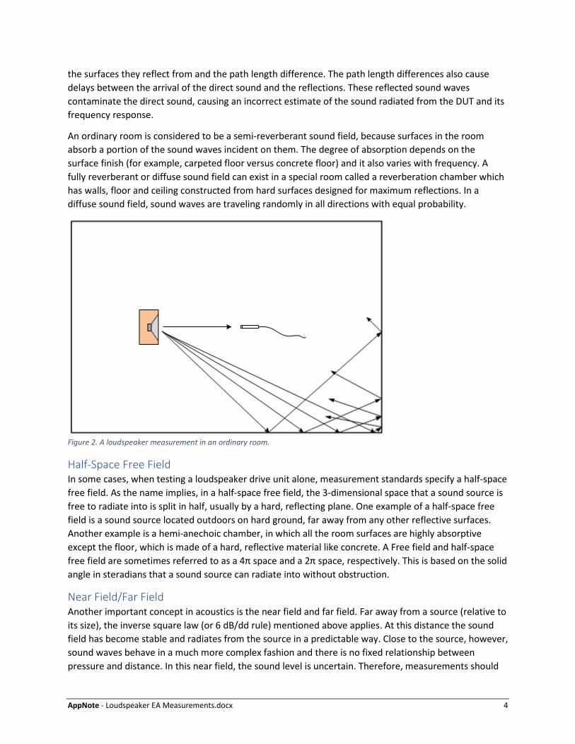
If instead, the loudspeaker and microphone are located in an ordinary room, in addition to measuring the direct sound, the microphone will measure sound reflected from the floors, walls, ceiling and any large objects within the room (Figure 2). The direct sound will arrive first at the microphone, followed by the first reflections from the closest surfaces and then secondary and tertiary reflections. Relative to the direct sound, the reflected sound waves will be lower in level depending on the absorptive properties of


the surfaces they reflect from and the path length difference. The path length differences also cause delays between the arrival of the direct sound and the reflections. These reflected sound waves contaminate the direct sound, causing an incorrect estimate of the sound radiated from the DUT and its frequency response.

An ordinary room is considered to be a semi-reverberant sound field, because surfaces in the room absorb a portion of the sound waves incident on them. The degree of absorption depends on the surface finish (for example, carpeted floor versus concrete floor) and it also varies with frequency. A fully reverberant or diffuse sound field can exist in a special room called a reverberation chamber which has walls, floor and ceiling constructed from hard surfaces designed for maximum reflections. In a diffuse sound field, sound waves are traveling randomly in all directions with equal probability.

Figure 2. A loudspeaker measurement in an ordinary room.

Half-Space Free Field In some cases, when testing a loudspeaker drive unit alone, measurement standards specify a half-space free field. As the name implies, in a half-space free field, the 3-dimensional space that a sound source is free to radiate into is split in half, usually by a hard, reflecting plane. One example of a half-space free field is a sound source located outdoors on hard ground, far away from any other reflective surfaces. Another example is a hemi-anechoic chamber, in which all the room surfaces are highly absorptive except the floor, which is made of a hard, reflective material like concrete. A Free field and half-space free field are sometimes referred to as a 4π space and a 2π space, respectively. This is based on the solid angle in steradians that a sound source can radiate into without obstruction.

Near Field/Far Field Another important concept in acoustics is the near field and far field. Far away from a source (relative to its size), the inverse square law (or 6 dB/dd rule) mentioned above applies. At this distance the sound field has become stable and radiates from the source in a predictable way. Close to the source, however, sound waves behave in a much more complex fashion and there is no fixed relationship between pressure and distance. In this near field, the sound level is uncertain. Therefore, measurements should


be conducted in the far field. The distance from the source to the far field depends on the size of the source. As a “rule of thumb” it is typically considered to begin at a distance of 3 times the largest dimension of the source [5]. However, it has been suggested that the far field begins at 3 to 10 times the largest dimension of the source [6].

Free Field Measurements To achieve free field conditions, two options are available: testing outdoors or in an anechoic chamber.

Outdoors To achieve free field conditions outdoors, a loudspeaker and microphone must be elevated high above the ground to minimize the influence of ground reflections. For example, the loudspeaker could be mounted on a tall tower, suspended from a crane, or on a boom projecting from the corner of a building’s roof. The required height depends on the size of the loudspeaker which in turn determines the required distance for the microphone to be in the far field. For example, consider a bookshelf-sized loudspeaker cabinet whose largest dimension is 0.33 m (13 in). Using the lowest rule of thumb value for the far field distance of three times the largest dimension of the source would require the microphone to be 1 m (3.28 ft.) away from the loudspeaker. Based on the 6 dB per doubling of distance rule, to reduce the level of reflected sound to 20 dB less than the direct sound would require a height of 5 m (16.4 ft.) above the ground. Doubling the size of this bookshelf speaker would double the height required to get the same 20 dB reduction of reflected to direct sound.

Obviously, conducting measurements with a loudspeaker and microphone located at 5 to 10 m (16 to 33 ft.) above ground is challenging! In addition to the inconvenience, inclement weather and ambient noise from wind, traffic, etc. can be problematic.

Half-space measurements can be conducted outdoors by using the ground as the reflective plane. In this case, the loudspeaker would be mounted in a baffle that is flush with the ground surface.

Anechoic Chambers An anechoic chamber is a special room lined with highly absorptive material on its interior surfaces – walls ceiling, floor and doors (Figure 3). To improve absorption at lower frequencies, the absorptive material (Fiberglas or open cell foam) is formed into wedges, with the wedge tips facing into the room. In fully anechoic (4π) chambers, an acoustically transparent working surface above the absorptive floor wedges is usually provided by means of an open, steel wire mesh suspended from the walls.

An anechoic chamber approximates a free field above a lower limiting frequency determined mainly by the length of its absorptive wedges. This lower frequency limit can be estimated from another rule of thumb: to absorb sound of a given frequency, the significant dimension of an absorptive material must be at least ¼ of the wavelength. Based on the ¼ wavelength rule and the speed of sound in air at room temperature (344 m/s or 1,129 ft./s), 1 m (3.28 ft) long wedges can effectively absorb sound above about 86 Hz in frequency. For practical reasons (and cost, of course), it is rare to find an anechoic chamber with a lower limiting frequency below 60 to 80 Hz. Chambers can be calibrated to lower frequencies using a loudspeaker system with sufficient bass (e.g., a subwoofer) with known frequency response. The challenge, then becomes finding the frequency response of this reference subwoofer.


It’s interesting to note that anechoic chambers are qualified in terms of how closely they adhere to the inverse square law or 6 dB/dd rule. The ISO standard covering sound power measurements in an anechoic chamber [7] specifies that measurements along traverse lines within the chamber must not deviate from the inverse square law by more than 1.0 to 1.5 dB, depending on frequency. And IEC 60268-5 [1] specifies that a chamber must be within ±10% of the inverse square law in the region between the loudspeaker and the microphone.

Figure 3. An anechoic chamber. Note the wedges on the inside of the open door and the suspended wire mesh floor. The wedges are 1.2 m (4 ft.) long. (Courtesy of Eckel Noise Control Technologies, Microsoft)

A low level of ambient noise is also desirable in an anechoic chamber, to enable measurement of low level harmonic distortion from loudspeakers as well as the sound emitted from low-level noise sources like display screens and electronic components. To minimize ambient noise, the best anechoic chambers are designed as an inner anechoic room inside an outer room. In addition, the inner room is often mounted on flexible vibration isolators to minimize structure-borne noise transmission from the outer room to the chamber. The chamber shown in Figure 3 recently set the new world record for the quietest location on earth, with an ambient noise level of -20.3 dBSPL.

Quasi-Anechoic Measurement Techniques Due to the expense of and limited access to anechoic chambers, much work has been devoted to the development of “quasi-anechoic” measurement techniques which seek to enable measuring the frequency response of loudspeakers (and microphones) in an ordinary, semi-reverberant room. These techniques are all time-selective; they work by stimulating the loudspeaker with a broad-band signal and analyzing that portion of the measured response that contains the direct sound from the loudspeaker but excludes the portion containing reflections from the room surfaces.


Quasi-anechoic techniques take advantage of one of the foundations of signal processing – the equivalence of a linear system’s frequency response and its impulse response. In the frequency domain, a system’s frequency response, H(f) represents its output magnitude and phase (or real and imaginary parts) per unit input, as a function of frequency. In the time domain, its impulse response, h(t), represents the system’s output as a function of time when stimulated by a unit impulse or Dirac delta function. These two representations of a dynamic system are equivalent, and one can be derived from the other using Fourier analysis. For example, the Fourier transform of the impulse response yields the frequency response. Similarly, the inverse Fourier transform of the frequency response yields the impulse response.

So how do time selective techniques work in practice? Consider the measurement setup depicted in Figure 4. A measurement microphone is positioned on-axis in front of a loudspeaker in a semi-reverberant room. To be in the far field of the loudspeaker, the distance d is chosen such that it is more than 3 times M, the largest significant dimension of the loudspeaker. The path length of the direct sound from the loudspeaker to the microphone is d, and the path length of the first reflection from the nearest reflecting surface (the floor in this case) is 2dR. Based on this geometry, the time difference, T, between

the direct sound arrival at the microphone and the first reflection is 𝑇𝑇 = 2𝑑𝑑𝑅𝑅−𝑑𝑑𝑐𝑐

, where c is the speed of sound.

Figure 4. A loudspeaker measurement on-axis in a semi-reverberant space.

Figure 5 (upper graph) shows an impulse response measured 1.17 m (3.84 ft.) in front of a bookshelf speaker located 2.86 m (9.4 ft.) above the floor in a large room. The peak in the impulse response occurs at about time t = 3.5 milliseconds (ms), which corresponds to the direct path length (1.17 m) divided by the speed of sound (334 m/s). Although it’s difficult to see in the impulse response, there are small secondary peaks that occur at time t = 16.5 ms and later. These smaller peaks, which are due to the arrival of reflections from the floor, walls and other room surfaces are much easier to see in the lower graph in Figure 5, which is called the Energy Time Curve (ETC). The ETC, which was introduced in the 1960s [9], is essentially a plot of the envelope of the impulse response. It’s plot of magnitude on a logarithmic scale makes it much easier to see the arrival time of room reflections.


Figure 5. A measured Impulse Response (top) and Energy Time Curve (bottom).

Time-selective or quasi-anechoic measurements would apply a window to the impulse response, eliminating any data after the first reflection arrives (about 15 ms, in this case), and then use a Fourier transform to compute the frequency response magnitude and phase (Figure 6). Typically, a rectangular window with cosine tapers at the beginning and end is used, to create smooth transitions. In Figure 6, the frequency response magnitude has been multiplied by the magnitude of the voltage signal applied to the loudspeaker, to determine the RMS Level in dBSPL.

Figure 6. RMS Level and Phase response computed from the Impulse Response in Figure 5 after windowing.


Obtaining the Impulse Response To use time-selective measurement techniques, one must first obtain the impulse response of a loudspeaker as set up in the test room. There are several methods available, each having certain advantages and disadvantages.

Impulse Testing The most direct way of obtaining the impulse response is to measure it directly through impulse testing. This involves applying a narrow (e.g., 10 µs wide) voltage pulse to the loudspeaker and measuring its response with a microphone. A sufficiently large room is required such that the direct response from the loudspeaker has substantially decayed by the time the first room reflection arrives at the microphone. The energy in the pulse is spread over a wide frequency range, resulting in a low signal to noise ratio (SNR), particularly at low frequencies, even with a pulse several tens of volts in magnitude. As a result, many averages must be used to improve the SNR. Impulse testing was first developed in the 1970s [8]. It has largely been replaced by other measurement techniques.

Maximum-Length Sequence Measurements The MLS method of measuring an impulse response was originally presented by Borish and Angell in 1983 [12]. A maximum length sequence (MLS) is a type of pseudo-random binary sequence. It can be specified in terms of its order N, where N represents the number of binary digits (or shift registers) used to create the sequence. An MLS of order N has a length of 2𝑁𝑁 − 1, and contains every possible combination of the binary values 0 or 1 in its N digits, (except the zero vector, in which all digits are 0). An MLS has some interesting properties which make it well suited to measuring impulse responses [10]. For practical purposes in audio testing, MLS signals are made symmetric (i.e., they are scaled to have values of +1 or -1 instead of 0 or 1).

One interesting property of a raw MLS signal is its crest factor (ratio of peak to rms level): All samples have a value of either +1 or -1 with a random distribution. Hence, the peak value and the rms value are both 1.0, resulting in a crest factor of 1.0, or 0 dB. This result only applies to a raw MLS, however. Once an MLS signal is passed through filters present in a typical audio measurement chain, the waveform is modified considerably, and its crest factor approaches a nominal 11 dB [10].

In loudspeaker testing, the MLS technique is based on exciting the DUT with an MLS and measuring its output. The impulse response is obtained by circular cross correlation of the measured output with the MLS signal input to the DUT. Once the impulse response has been derived, like any quasi-anechoic technique, it can be windowed to remove the portion containing reflections, and then Fourier transformed to yield an estimate of the DUT’s transfer function. By nature, an MLS signal is spectrally flat (like white noise). The signal is often filtered to have a pink noise spectrum (i.e., the rms level decreases linearly with frequency), which is more suitable for acoustic systems.

One of the advantages of MLS testing over other techniques is that, when averaging is used, it has relatively high immunity to steady or impulsive noise that is not correlated with the MLS input sequence. A disadvantage, however is that it is impossible to separate the linear response of the system from nonlinearities, such as harmonic distortion. Loudspeakers always have relatively high levels of distortion compared to electronic systems. In an impulse response measured via MLS, this distortion and other nonlinearities appear as artifacts or peaks distributed along the impulse response.


Log-Swept Sine Measurements A sine signal with continuously varying frequency is often called a chirp. Linearly-swept sine chirps, wherein the sine frequency varies linearly with time, have been used in audio test for many decades, including in Time Delay Spectrometry (TDS). TDS is another well-known quasi-anechoic measurement technique, first introduced in 1967 [13]. These methods are also subject to the limitation that non-linear effects such as distortion cannot be separated from the system’s linear response.

The value of chirp signals changed dramatically when the first logarithmic chirp technique was introduced by Farina in 2000 [14]. He discovered that when a log-swept sine chirp signal is used to stimulate a system, through deconvolution, it is possible to simultaneously derive the linear impulse response of the system as well as separate impulse responses for each harmonic distortion component. For example, Figure 7 shows the result of deconvolution of the signal from an analog graphic equalizer stimulated with a log-swept sine chirp [16]. The linear system impulse response is shown at time zero, and the impulses of the harmonic distortion components appear logarithmically spaced in negative time. By carefully time-windowing and Fourier transforming the various impulses, the individual response functions can be recovered, from which many different measurements can then be derived mathematically. In other words, almost every common audio measurement can be obtained from a single, fast acquisition, dramatically decreasing test time.

Figure 7. Impulse response derived by deconvolution following a chirp measurement of an analog graphic equalizer. The amplitude axis has been enlarged to show the harmonic distortion impulses [16].

Farina’s original paper focused on measuring the response of rooms and loudspeakers. Müller and Massarini [15], motivated by the requirement to measure high quality room impulse responses, showed that the log-swept sine chirp method is preferable to MLS for room measurements as well as for most DUTs, including electro-acoustic devices. Kite [16] demonstrated that log chirp measurements of audio devices provide comparable results to traditional swept sine measurements and suggested an extension to measure crosstalk. The extension involves staggering the stimulus signals applied to each channel of a DUT such that each channel is offset from the previous one by a short time. This enables crosstalk to be measured simultaneously with frequency response and distortion.


The log-swept sine chirp measurement became a hallmark of Audio Precision’s APx500 audio analyzer platform, first introduced in 2006 with the launch of the APx585 8-channel audio analyzer. Since its introduction, the APx platform has had two chirp measurements intended for electronic audio test, named Continuous Sweep and Frequency Response. The Continuous Sweep measurement provides a multitude of audio results including level, gain, phase, harmonic distortion, group delay, crosstalk, impulse response and more. The Frequency Response measurement contains a subset of these results for users who simply want to quickly measure a device’s level and gain versus frequency, and its deviation from flatness. In 2009, a version of the log-swept chirp measurement specifically intended for testing acoustic devices was added to the APx platform. The measurement, named Acoustic Response, includes an Energy Time Curve result, controls for windowing out acoustic reflections for quasi-anechoic analysis, and several results of interest to users testing loudspeakers.

Limitations of Quasi-Anechoic Measurements As mentioned above, quasi-anechoic techniques work by windowing out the portion of the impulse response containing room reflections. Sometimes, this windowing truncates the impulse response before it has decayed to a sufficiently negligible level. This truncation causes errors in the estimated frequency response, especially at low frequencies. For example, consider a situation in which the impulse response is windowed 5 ms after its peak value. This would be a typical value for a small (bookshelf-sized) speaker measured in a room with a 2.74 m (9 ft.) high ceiling. With a measurement distance of d = 1.0 m and the distance h = 1.36 m (4.45 ft) to the nearest reflecting surface, the first reflection would arrive about 5.5 ms after the direct sound. Hence the impulse response might be windowed to a length of 5.0 ms.

Figure 8. Frequency response of a loudspeaker derived from an impulse response with no window (solid blue trace) and a 5 ms window (dashed orange trace).

Figure 8 illustrates the effect of windowing one loudspeaker’s measured impulse response at 5 ms after the peak. This data is from a measurement in a small acoustically lined hearing aid test box with an integrated full-range loudspeaker. Although this test setup would preclude an accurate measurement of this loudspeaker’s response at low frequencies, Figure 8 does show the dramatic impact of windowing the impulse response. The windowed response is radically different from the un-windowed response below about 300 Hz, and the smoothing effect of the window is apparent up to about 1 kHz. With a


window width of T = 5 ms, the resolution in the frequency domain is about 1/T = 200 Hz. In the graph, the shaded region below 200 Hz is intended to indicate that the curve is unreliable in this region. But, note that the effect of windowing extends to a much higher frequency than 200 Hz.

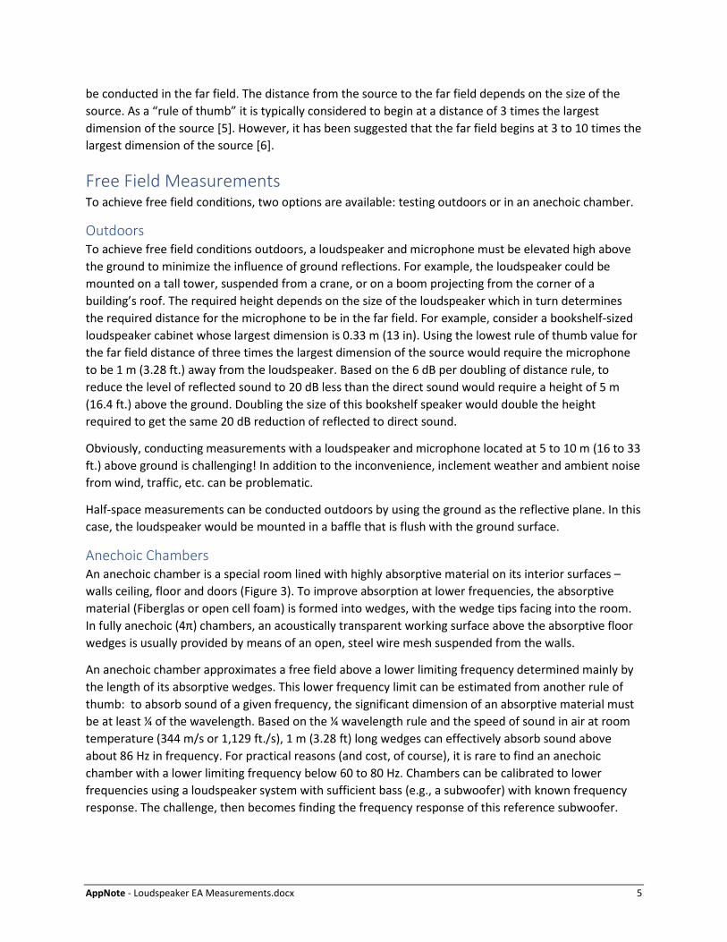
The duration of a loudspeaker’s impulse response depends mainly on its low-frequency roll off characteristics [17]. To see this in an acoustical measurement, would require an impulse response measured in a perfectly anechoic environment with low ambient noise – difficult to obtain. However, the low-frequency behavior of a loudspeaker system can easily be modeled based on its resonant frequency and other parameters derived from simple electrical measurements of the system impedance. For example, Figure 9 shows the impulse response of an ideal small vented box system with a 127 mm (5 in) diameter low frequency driver. The impulse response is shown with a tapered rectangular window that ends 10 ms after the peak. In the right half of the figure, the vertical scale has been increased by a factor of 40, to show the detail in the tail of the impulse response. As shown, a 10 ms window would severely truncate the impulse response. The corresponding frequency response magnitude for the un-windowed and windowed impulse response is shown in Figure 10. Note the errors below 100 Hz and the ripples in the response for the windowed impulse response.

Figure 9. Impulse response of a small vented box loudspeaker (blue trace) with a tapered window 10 ms after the peak, normal viewing scale (left) and vertical scale zoomed 40 x (right).

Figure 10. Frequency response calculated from the un-windowed (solid blue trace) and windowed (dashed red trace) impulse response of Figure 9.

Figure 9 indicates that the tail of the impulse response has not decayed until 30 to 40 ms after the peak. It would require an impractically large room to ensure that reflections were delayed by 30 ms after the direct sound!


Methods of extending quasi-anechoic techniques to lower frequencies by shortening a loudspeaker’s impulse response have been proposed by Fincham [17] and more recently by Backman [18]. These appear to be effective. However, because their application requires modeling the loudspeaker’s low frequency response, Vanderkooy and Lipschitz [19] suggest that these impulse shortening techniques should not really be considered as measurement methods.

Combining Near Field and Far Field Measurements One approach to overcoming the inaccuracy of quasi-anechoic techniques at low-frequencies involves combining them with near-field measurements. Keele [19] demonstrated that the far field frequency response of a loudspeaker at low frequencies can be estimated by measurements in the near field. This relationship is valid at low frequencies, at which the driver behaves like a rigid piston. In practice, the measurement microphone must be placed very close to the dust cap of the driver. Theoretically, to be within 1 dB of the true near field pressure, the microphone must be within 0.11𝑟𝑟 of the dust cap, where 𝑟𝑟 is the driver radius. For example, for the 127 mm (5 in) diameter driver listed above, the microphone would need to be less than 7 mm (0.28 in) from the dust cap. At this close distance, reflections and noise are essentially eliminated.

Figure 11. Graphic illustrating the technique of combining near field and far field measurements to obtain full-range frequency response (excluding diffraction effects).

Struck and Temme [20] presented a method whereby a loudspeaker’s full-range frequency response is derived by combining its low-frequency response as measured by the near field technique with its high-frequency response as measured using a quasi-anechoic technique. This is illustrated in Figure 11. The far field quasi-anechoic measurement is conducted at some distance greater than 3𝑀𝑀, where M is the most significant dimension of the loudspeaker enclosure. This measurement provides data that is useful at frequencies greater than 1/𝑇𝑇, where T is the length of the time window applied to the impulse response to eliminate room reflections. The near field measurement is conducted with the microphone very close to the driver. This measurement is valid at frequencies below 𝑓𝑓 = 𝑐𝑐/𝜋𝜋𝑀𝑀1, where 𝑐𝑐 is the

1 Note: This frequency limit is for a driver mounted in an infinite baffle. For a driver in a cabinet, the upper frequency limit will be lower.


speed of sound and 𝑀𝑀 is the significant cabinet dimension. The near field measurement results in a frequency response curve that is much higher in level than the far field response. The curves are combined by shifting the near field response curve down in level such that it matches the far field curve at some point in the overlap region and splicing the curves together. The overlap region is the frequency range between 1/𝑇𝑇 and 𝑐𝑐/𝜋𝜋𝑀𝑀.

For the near field / far field splice technique to work, the room must be large enough relative to the size of the loudspeaker for there to be an overlap frequency range. In addition, if the loudspeaker system has one or more ports or multiple drivers, the technique becomes more complicated: A near field measurement of each driver and port must be made and these must be summed in the complex domain (i.e., with regard to magnitude and phase) after first scaling the component responses to account for their different radiating surface areas.

Diffraction Effects A disadvantage of using a near field measurement to estimate the low-frequency response of a loudspeaker enclosure in the far field is that it does not include the effects of diffraction from the enclosure edges, sometimes referred to as baffle step diffraction. This effect causes an apparent “loss” at low frequencies and ripples in the frequency response at higher frequencies which are not present when the driver is mounted in an infinite baffle.

In simple terms, the baffle diffraction effect can be explained as a transition from 4π space to 2π space radiation as the wavelength of sound decreases with increasing frequency. At low frequencies, where the wavelength is long compared to the baffle dimensions, the baffle is acoustically transparent, and the sound radiates into 4π space. At high frequencies, where the wavelength is short compared to the baffle dimensions, a driver radiates into a half-space (or 2π space). As a result, the overall mean sound pressure is twice the level (or 6 dB higher) at high frequencies.

In addition to the overall 6 dB increase in the mean level, in the transition region between high and low frequencies, the baffle diffraction effect causes peaks and dips in the response curve that vary depending on the baffle shape and dimensions, and the position of the driver on the baffle. In a seminal paper on the subject published in 1951, Olsen [28] demonstrated measured diffraction response for 12 different enclosure shapes.

Figure 12. Estimated Diffraction effect for a closed box bookshelf speaker with 127 mm driver mounted in the center of a 197 x 294 mm rectangular baffle.

If enclosure diffraction effects are not accounted for, the near field / far field splice technique described above can cause errors in the estimated frequency response. Luckily, there are software tools available to simulate baffle diffraction. For example, Figure 12 shows the baffle diffraction estimated with a


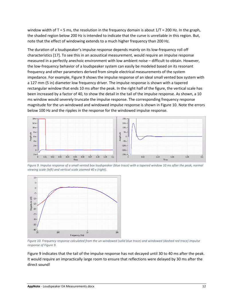
program call the Edge, from Tolvan Data [29] for a rectangular loudspeaker enclosure with a 127 mm driver mounted in the middle of its 197 x 294 mm front baffle. Figure 13a shows three frequency response curves for the same loudspeaker system - the measured near field response, the quasi anechoic far field response measured using a 5 ms time window, and the near field response combined with the simulated diffraction response shown in Figure 12. Figure 13b shows the results of splicing the near field / far field response curves with and without the estimated diffraction response. Note that without the estimated diffraction (red trace in Figure 13b) the spliced curve is significantly off at low frequency.

Figure 13. (a) Relative response (left) of near field measurement, diffraction corrected near field measurement and far field measurement. (b) Combined near/far field response with and without diffraction correction.

Ground-Plane Measurements Another approach to approximating the free field response of a loudspeaker is the ground-plane measurement technique [30]. This technique takes advantage of the fact that the acoustic reflection from a loudspeaker placed directly on a hard, reflective surface is predictable.

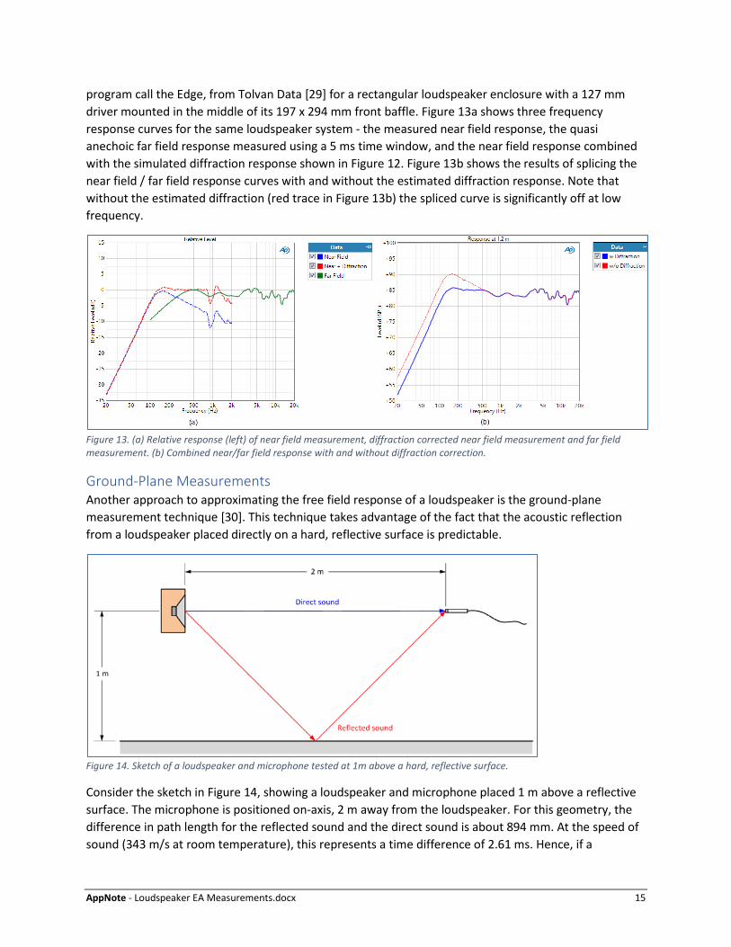
Figure 14. Sketch of a loudspeaker and microphone tested at 1m above a hard, reflective surface.

Consider the sketch in Figure 14, showing a loudspeaker and microphone placed 1 m above a reflective surface. The microphone is positioned on-axis, 2 m away from the loudspeaker. For this geometry, the difference in path length for the reflected sound and the direct sound is about 894 mm. At the speed of sound (343 m/s at room temperature), this represents a time difference of 2.61 ms. Hence, if a


sinusoidal signal is generated by the loudspeaker, two sine signals of the same frequency and essentially the same amplitude will arrive at the microphone, but the reflected sound will be delayed by 2.61 ms. This time delay represents a phase shift. At some frequencies, the signals will be 180 degrees out of phase and they will completely cancel out. At frequencies two times higher, the signals will be exactly in phase, and their combined amplitude will be twice that of the direct sound, or 6 dB higher in level. This causes a comb filter effect at the microphone position, as shown in Figure 15. As shown, for this geometry, the signals completely cancel out at multiples of 192 Hz, and they sum to twice the amplitude of the direct sound at multiples of 384 Hz.

Figure 15. The comb filter effect caused by interference between the reflected sound and direct sound for the geometry shown in Figure 14.

As the loudspeaker and measurement microphone are moved closer to the reflecting plane, the path length difference decreases, causing the notches of the comb filter to occur at higher frequencies. In the limiting case, the loudspeaker and the microphone are placed directly on the ground plane, and the speaker is tilted such that the reference axis points directly at the microphone. For a standard ½” measurement microphone, the center of the microphone’s diaphragm will be about 6.4 mm above the ground plane when the microphone is directly on the surface. For a loudspeaker height of 40 cm, the first notch in the comb filter would be at about 68 kHz, resulting in a level response 6 dB higher than the direct sound up to 20 kHz. As the source height increases, the frequency of the first notch will decrease, limiting the upper frequency range of ground plane measurements to a frequency below 20 kHz. One way to mitigate this effect is to place the high-frequency driver closer to the ground (i.e., to invert a loudspeaker system with the tweeter at the top of the baffle.

Figure 16. A ground plane measurement. The speaker is tilted toward the microphone, which is 2 m away. The reflected sound can be thought of as a mirror image of the speaker located symmetrically below the reflecting plane.

As shown in Figure 16, from the perspective of the microphone, it “appears” that there is a second identical loudspeaker located symmetrically with respect to the ground plane. At frequencies below the first notch in the comb filter, the signals will be in phase and will have a combined level 6 dB higher than the level of the direct sound. This can be used to advantage by placing the microphone at a distance two


times the intended measurement distance. For example, a common specification is the frequency response measured on-axis at 1 m distance due to a sinusoidal stimulus of 1 W. Assuming the loudspeaker is small enough that 1 m is in the free field of the DUT, a ground plane measurement at 2 m will yield the same level response as a free field measurement at 1 m.

Figure 17 shows a ground plane measurement of a small bookshelf speaker in a large open field and the resulting frequency response measured at 2 m due to 1 W input. In this case, the loudspeaker and microphone were placed on a table top resting on the ground, to ensure a reflective surface.

Figure 17. A bookshelf speaker measured using the ground plane technique and the resulting frequency response at 2 m.

Ground plane measurements offer an inexpensive alternative to an anechoic chamber, but they still have some issues. One issue is diffraction; due to the reflected image of the loudspeaker, the baffle appears to be twice as high as it really is, causing a different diffraction response along the edge in contact with the ground. Also, a large open area is required with no vertical reflecting surfaces located within about 10 m of the loudspeaker. And, of course ambient outdoor noise from vehicles, machinery, aircraft and the wind is usually of concern, especially for low-frequency measurements where the output of the DUT is relatively low.

Standard Loudspeaker Measurements Measurement Conditions IEC 60268-5 specifies how loudspeakers are to be set up for measurement.

Rated Conditions To determine the correct conditions for conducting measurements, IEC 60268-5 specifies several properties known as Rated Conditions that should be taken from manufacturer’s specifications. These properties do not need to be measured, but other measurement characteristics are based on their values. Rated Conditions are listed in Table 1.

Table 1. Rated Conditions to be specified by the manufacturer

Condition Description Rated Impedance The nominal value of a pure resistance used to define the

power of the amplifier driving the speaker.


Condition Description Rated Sinusoidal Voltage or Power The voltage of a sinusoidal signal within the rated frequency

range that the loudspeaker can handle continuously without sustaining thermal or mechanical damage.

Rated Noise Voltage or Power The voltage of a program simulation noise signal that the loudspeaker can handle continuously without sustaining thermal or mechanical damage.

Rated Frequency Range The range of frequencies that the loudspeaker is intended to be used within.

Reference Plane A plane used to define the Reference Point and Reference Axis, usually parallel to the front radiating surface.

Reference Point A point on the Reference Plane used to define the Reference Axis (usually a point of symmetry for symmetric structures).

Reference Axis A line passing through the Reference Plane at the Reference Point to be used as the zero axis for frequency response and directivity measurements.

Normal Measuring Conditions IEC 60268-5 specifies several conditions which are required for measurements. These include:

• Mounting • Acoustical Environment • Loudspeaker and Microphone Position • Test Signal

Mounting The performance of a loudspeaker drive unit (or driver) depends on the properties of the unit itself and its acoustic loading, which in turn, depends on its mounting arrangement. Drive units may be mounted in one of three configurations, with the selected configuration clearly described in the test results:

1. A standard baffle or in one of two specified standard measuring enclosures. 2. In free air without a baffle or enclosure. 3. In a half-space free field, flush with the reflecting plane

Loudspeaker systems are usually measured without any additional baffle. The manufacturer can specify that a baffle be used, in which case a description of the mounting arrangement should be included with the test results.

Acoustical Environment IEC 60268-5 requires that measurements be made in one of 5 specified acoustic fields:

1. Free-field Conditions: In an anechoic chamber, the minimum requirement for a free field is considered to exist if sound propagation from the source follows the 6 dB/dd rule within ±10% on the axis between the Reference Point and the measurement microphone.

2. Half-Space Free-field Conditions: In a half-space free-field, reflecting plane should be large enough that 6 dB/dd rule is met within ±10% between the surface and the measurement microphone.


3. Diffuse Conditions: If a diffuse sound field is used (e.g. a reverberation chamber), measurements should be conducted with 1/3-octave band limited noise.

4. Simulated Free Field Conditions: This refers to the use of quasi-anechoic techniques and specifies that a large unobstructed room be used such that any reflections arrive after the direct sound has decayed. The standard only refers to the impulse testing technique, but presumably other quasi-anechoic techniques can be used.

5. Simulated Half-Space Free Field Conditions: This condition is the same as 4, above, except that the quasi-anechoic technique simulates a half-space free field.

The acoustic field type chosen for the tests should be clearly indicated with the test results.

Loudspeaker and Microphone Position IEC 60268 specifies that ideally, measurements in free field and half-space free field conditions should be conducted with the measurement microphone in the far field of the loudspeaker. However, it notes that in practice, imperfections in the anechoic chamber and the effects of background noise may impose an upper limit on the distance from loudspeaker to microphone. The measurement distance should therefore be either 0.5 m or an integer number of meters, with the result being referred to 1m.

For single drive units, IEC 60268-5 specifies a measurement distance of 1 m, unless conditions dictate a different value.

For simulated free field conditions, IEC 60268-5 specifies the same measurement distance requirement as for free field conditions, with the added caveat that the loudspeaker and microphone should be positioned within the measurement room to maximize the time between the direct sound and the first reflection. It also states that any errors in the measured frequency response due to truncation should not exceed 1 dB over the frequency range of interest.

Test Signal IEC 60268-5 specifies that one of the following types of test signals be used:

• A sinusoidal signal not exceeding the rated sinusoidal voltage at any frequency. The voltage across the loudspeaker input terminals should be kept constant at all frequencies.

• A broadband noise signal with a crest factor between 3 and 4. • A narrow-band noise signal consisting of pink noise filtered in 1/3-octave bands. • An impulsive signal (for impulse testing).

Measurement Equipment IEC 60268-1 specifies that a microphone with known calibration should be used. The recommended practice for free field measurement conditions is to use a free field measurement microphone2. These calibrated microphones are stable and have a flat frequency response over a wide frequency range. For greater precision, the audio analyzer’s input equalization (EQ) feature can be used to eliminate any

2 Note: In section 8, IEC 60268-5 indicates that a pressure microphone should be used. This is a holdover from a much earlier time when the frequency response correction for a free field microphone was uncertain [2]. Current recommended practice is to use a free field microphone for free field measurements.


deviations from flatness from the measured response. For diffuse field conditions, a random incidence measurement microphone should be used.

The standard also specifies that the signal generator, the power amplifier used to drive the loudspeaker and the microphone measurement system have a flat frequency response within ± 0.5 dB. AP audio analyzers easily meet this requirement, as does the APx1701 Transducer Test Interface (Figure 14). This loudspeaker test accessory is equipped with instrumentation quality power amplifiers configured as two independent channels, with power ratings up to 100 W for a single channel into 8 Ω, flat frequency response from DC to 100 kHz, low output impedance, built-in current sense resistors and support for pre-polarized and phantom-powered measurement microphones.

Figure 18. The APx1701 Transducer Test Interface.

Positive Terminal In section 14, IEC 60268-1 specifies that a driver’s terminals be marked as positive and negative. A test for correct marking is conducted by measuring the sound pressure level in front of the drive unit while applying a positive DC voltage to the positive terminal. The measured sound pressure level should increase when the DC voltage is applied, as shown in Figure 15.

Figure 19. Sound pressure waveform measured in the near field of a driver subjected to a voltage step of +1 Vdc.


Impedance and Derivative Characteristics Rated Impedance As stated above, the rated impedance of a loudspeaker is the nominal value of a pure resistance used to define the power required to drive the speaker. Although a nominal resistance value is used, a loudspeaker impedance is a phasor or complex quantity (it has both magnitude and phase), and it varies significantly over the audio frequency range. For example, Figure 16 shows the impedance magnitude of a 3-way loudspeaker system from 20 Hz to 20 kHz. The three peaks in the curve are resonant frequencies associated with the three drivers in the system.

Figure 20. Impedance magnitude of a 3-way loudspeaker system with nominal impedance = 8 ohms.

IEC 60268-5 specifies that the lowest value of the impedance magnitude within the rated frequency range shall not be less than 80% of the rated impedance. The standard also requires that if the impedance at any frequency outside the rated frequency range (including DC) is less than 80% of nominal impedance, this should be stated in the specifications. Note that the minima in the impedance curve of Figure 20 are just below 6 ohms for this nominal 8-ohm system, indicating that this system does not meet the rated impedance requirement of IEC 60268-5.

Impedance Curve IEC 60268-5 requires that the impedance magnitude curve be measured over the standard audio frequency range (20 Hz to 20 kHz). For drive units, IEC 60268-5 indicates that the driver should either be mounted in a standard baffle or in free air. When comparing the impedance of drive units, care should be taken to ensure that the same mounting method is used, because the mounting method could have a significant impact on the measured impedance.

Impedance is measured by applying a constant voltage versus frequency to the loudspeaker and measuring the voltage at the input terminals as well as the current. The log-swept chirp signal is a good stimulus for impedance measurements. Typically, the current is measured by sensing the voltage drop across a small sense resistor in series with the loudspeaker, as shown in Figure 17-a. Impedance measurements are easy with the APx1701 Transducer Test Interface (Figure 14), which has a built-in current sense resistor in the ground leg of each power amplifier circuit. For those not using an APx1701, Figure 17-b shows a handy accessory for making impedance measurements. It has two selectable sense


resistors and connectors that facilitate easy connection of the loudspeaker and power amplifier to the audio analyzer.

Figure 21. (a) Schematic of a typical impedance measurement. (b) IMP1 Impedance Test Fixture.

The drive level used for impedance measurements can have a strong influence on the accuracy of results. It should be low enough to ensure that the loudspeaker is operating well within its linear range, but high enough to ensure a good signal to noise ratio. Measurements at several different drive levels should be examined for consistency, to help choose an appropriate level.

Thiele-Small Parameters IEC 60268-5 calls out three loudspeaker drive unit characteristics that are derived from the impedance curve and defines them as follows:

1. The resonance frequency (FS): The frequency at which the first peak in the impedance magnitude occurs.

2. The Total Q-factor (QTS): the ratio of the inertial part of the acoustic or mechanical impedance to the resistive part of the impedance at the resonance frequency.

3. The Equivalent Air Volume of Compliance (Vas).

FS, QTS and VAS are just three of a larger set of electromechanical parameters used to characterize the low-frequency behavior of loudspeaker drivers. These parameters, are collectively named the Thiele/Small (T/S) parameters, after A.N. Thiele and R.H. Small, who published influential papers [21 – 24] showing how these parameters, derived from simple electrical impedance measurements, could be used to design loudspeaker enclosure systems.


Figure 22. Measured impedance magnitude (left) and phase (right) of an 8-ohm, 130 mm diameter driver. The model curve fit to the data is shown as a solid red trace.

IEC 60268-5 specifies some simple procedures for calculating QTS and VAS from the resonance region of the measured impedance magnitude. In modern systems like Audio Precision’s APx500 audio analyzers, the T/S parameters are derived by fitting an electromechanical model of the driver to the measured complex impedance curve. The impedance can be measured from 20 Hz to 20 kHz, as specified in the standard, with the curve fit concentrated on the region around resonance (Figure 18), which is most important to a good fit.

Audio Precision’s APx500 audio analyzers include a choice of three driver models from which to derive the T/S parameters: The Standard, LR-2 and Wright models (Table 2). In all three models, the moving mass of the driver is modeled as a resonant system, shown as the dotted box on the right of each circuit diagram in Table 2. The Standard model (a) assumes that the simple series resistance plus inductance of the voice coil accurately models the electrical impedance of the driver. In a practical system, eddy current losses in the magnet and pole piece cause the real part of the impedance to climb with frequency, which the Standard Model does not predict.

Table 2. Three electromechanical circuit models used to derive the Thiele-Small parameters.

(a) Standard Model

Thiele/Small Parameters Symbols & Units Symbol Unit Description

FS Hz Resonant frequency of the driver

QMS ---- Mechanical Q at Fs

QES ---- Electrical Q at Fs

QTS ---- Total Q at Fs

SD cm^2 Effective surface area of cone

RE ohm Voice coil resistance

LE mH Voice coil inductance

R2 ohm LR-2 model: voice coil parallel resistance

L2 mH LR-2 model: voice coil parallel inductance

Erm ---- Wright model: motor resistance exponent

Krm ---- Wright model: motor resistance coefficient

Exm ---- Wright model: motor reactance exponent

Kxm ---- Wright model: motor reactance coefficient

RMS Ns/m Mechanical resistance of suspension

CMS mm/m Mechanical compliance of the suspension

MMS gram Mechanical mass including air load

(b) LR-2 Model

(c) Wright Model


VAS liter Acoustic volume with same compliance as suspension

Bl Tm Magnetic motor strength

η0 % Reference efficiency of the driver

The LR-2 model [25] assumes that the network shown in Table 2-b in series with the mechanical impedance accurately models the electrical impedance of the coil, including eddy current losses. This model provides a more accurate fit to the measured impedance curve than the Standard model and can be implemented with physical components or digital filters.

The Wright model [26] assumes that the network shown in Table 2-c in series with the mechanical impedance accurately models the electrical impedance of the coil, including eddy current losses. This model provides a very accurate fit to the measured impedance curve, but it cannot be implemented with physical components or digital filters because it uses unrealizable parameters, such as fractional resistance and inductance. With certain software tools, the Wright model is useful in crossover and enclosure design.

To derive the full set of T/S parameters from a single impedance measurement in free air, the moving mass of the driver without air load (MMD) is required3. If MMD is unknown, it can be estimated by disassembling (which usually means destroying) the driver and weighing the moving components. If MMD is unknown and a driver cannot be spared to measure it, the full set of T-S parameters can also be estimated using one of two techniques that require a second measurement: The Added Mass or Known Volume techniques.

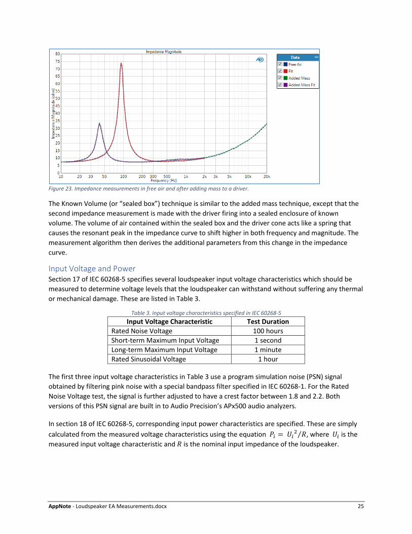
For the Added Mass technique, following the impedance measurement in free air, a second impedance measurement is conducted after adding a known mass to the driver. Typically, a toroid of “sticky” modeling clay is weighed on a precision scale and temporarily added to the driver cone surrounding the dust cap. This added mass causes the resonant peak in the driver’s impedance curve to shift lower in both frequency and magnitude (Figure 19). The measurement algorithm then derives the additional parameters from this change in the impedance curve.

3 Klippel and Seidel [27] demonstrated that the full set of T/S parameters can also be derived from a single measurement in free air when MMD is unknown, by measuring the driver displacement and impedance simultaneously.


Figure 23. Impedance measurements in free air and after adding mass to a driver.

The Known Volume (or “sealed box”) technique is similar to the added mass technique, except that the second impedance measurement is made with the driver firing into a sealed enclosure of known volume. The volume of air contained within the sealed box and the driver cone acts like a spring that causes the resonant peak in the impedance curve to shift higher in both frequency and magnitude. The measurement algorithm then derives the additional parameters from this change in the impedance curve.

Input Voltage and Power Section 17 of IEC 60268-5 specifies several loudspeaker input voltage characteristics which should be measured to determine voltage levels that the loudspeaker can withstand without suffering any thermal or mechanical damage. These are listed in Table 3.

Table 3. Input voltage characteristics specified in IEC 60268-5 Input Voltage Characteristic Test Duration

Rated Noise Voltage 100 hours Short-term Maximum Input Voltage 1 second Long-term Maximum Input Voltage 1 minute Rated Sinusoidal Voltage 1 hour

The first three input voltage characteristics in Table 3 use a program simulation noise (PSN) signal obtained by filtering pink noise with a special bandpass filter specified in IEC 60268-1. For the Rated Noise Voltage test, the signal is further adjusted to have a crest factor between 1.8 and 2.2. Both versions of this PSN signal are built in to Audio Precision’s APx500 audio analyzers.

In section 18 of IEC 60268-5, corresponding input power characteristics are specified. These are simply calculated from the measured voltage characteristics using the equation 𝑃𝑃𝑖𝑖 = 𝑈𝑈𝑖𝑖2 𝑅𝑅⁄ , where 𝑈𝑈𝑖𝑖 is the measured input voltage characteristic and 𝑅𝑅 is the nominal input impedance of the loudspeaker.


Frequency Response In section 21, IEC 60268-5 indicates that the frequency response shall be specified as measured under free field or half-space free field conditions at a stated position with respect to the reference axis and reference point, at a specified constant voltage.

Effective Frequency Range Section 21 also defines a characteristic called the Effective Frequency Range (EFR). The EFR is determined from a frequency response measurement conducted on the reference axis of the loudspeaker. It is derived by first finding the maximum sound pressure level averaged over a bandwidth of one octave and centered on the frequency of maximum sensitivity. Next, the lower and higher limiting frequencies are found at which the response is no more than 10 dB below the maximum sound pressure level. Sharp troughs in the response curve narrower than 1/9-octave are ignored when determining the EFR.

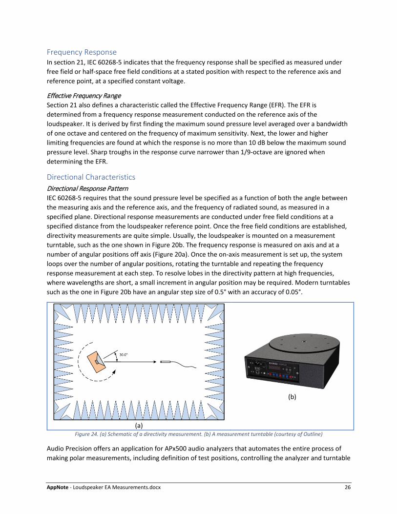
Directional Characteristics Directional Response Pattern IEC 60268-5 requires that the sound pressure level be specified as a function of both the angle between the measuring axis and the reference axis, and the frequency of radiated sound, as measured in a specified plane. Directional response measurements are conducted under free field conditions at a specified distance from the loudspeaker reference point. Once the free field conditions are established, directivity measurements are quite simple. Usually, the loudspeaker is mounted on a measurement turntable, such as the one shown in Figure 20b. The frequency response is measured on axis and at a number of angular positions off axis (Figure 20a). Once the on-axis measurement is set up, the system loops over the number of angular positions, rotating the turntable and repeating the frequency response measurement at each step. To resolve lobes in the directivity pattern at high frequencies, where wavelengths are short, a small increment in angular position may be required. Modern turntables such as the one in Figure 20b have an angular step size of 0.5° with an accuracy of 0.05°.

(a)

(b)

Figure 24. (a) Schematic of a directivity measurement. (b) A measurement turntable (courtesy of Outline)

Audio Precision offers an application for APx500 audio analyzers that automates the entire process of making polar measurements, including definition of test positions, controlling the analyzer and turntable


throughout the data collection and analyzing the measurement results. An example of measured polar response patterns for a loudspeaker system is shown in Figure 21. Note the irregularities in the otherwise omnidirectional response pattern at 125 Hz. This is likely due to inaccuracies in the free field conditions for the anechoic chamber used for these measurements.

Figure 25. Polar response of a loudspeaker in one plane at multiple frequencies as measured with 1° angular resolution with the APx Polar Plot Utility.

An alternative representation of directivity data is shown in Figure 22. In this 3-dimensional plot, sound pressure level is represented by color intensity on a plot of measurement angle versus frequency.

Figure 26. An alternative means of displaying directivity data. This plot shows the source data from the plot in Figure 21 imported to VACS software (courtesy R&D Team).


Amplitude Nonlinearity Section 24 of IEC 60268-5 covers distortion measurements, including harmonic distortion, modulation distortion and difference frequency distortion.

Harmonic Distortion For harmonic distortion measurements at input levels up to the rated sinusoidal voltage, IEC 60268-5 species that the loudspeaker be driven by a series of sinusoidal voltages with increasing frequencies up to 5 kHz. Measurements are conducted with a measurement microphone on-axis in a free field for loudspeaker systems or a half-space free field for drive units. The sound levels of individual harmonics are measured, as well as the overall sound level. Total Harmonic Distortion (THD) is calculated as the sum of all the harmonics expressed as a ratio to the overall sound level. The standard also specifies harmonic distortion of the second and third order, wherein the level of the 2nd and 3rd harmonics are expressed as a ratio to the overall sound level.

As discussed under Obtaining the Impulse Response, above, frequency response measurements conducted using the log-swept sine chirp stimulus have the advantage of providing harmonic components simultaneously with the main response, in one measurement. For example, Figure 23 shows the fundamental, 2nd order, 3rd order and total harmonic distortion levels on a single graph. Note that for this loudspeaker, 3rd order distortion dominates the THD up to about 3 kHz and 2nd order distortion is dominant at higher frequencies. Chirp measurements in Audio Precision’s APx platform include the ability to track individual harmonics up to the 20th order, as well as the sum of any combination of harmonics H2 through H20 (Figure 24).

Figure 27. A level and distortion graph measured in the near field of a loudspeaker, showing the level of the fundamental (F) and 2nd and third order distortion components (H2 & H3), and Total distortion level.


Figure 28. Plot of the 20th order (H20) and total harmonic distortion ratio (THD) for the measurement in Figure 23.

To test at signal levels higher than the rated sinusoidal voltage, IEC 60268-5 specifies a method whereby the loudspeaker is stimulated with a tone burst. A burst is usually conducted by generating a sine signal at some frequency and abruptly alternating the level between a high level and a lower level. For example, the left side of Figure 25 shows the signal acquired from a loudspeaker stimulated with a burst waveform at 1 kHz sine frequency, 40 ms at high level followed by 160 ms at a level 20 dB lower. By using this type of burst signal with, for example, a 25% duty cycle, the loudspeaker can be stimulated at a level higher than its rated voltage. A subset of the waveform acquired during the high-level portion of the signal can then be extracted and subjected to FFT analysis, as shown on the right side of Figure 25. The harmonic distortion components are extracted from the FFT spectrum and used to calculate the THD. In the case of this example, the measured THD was -54 dB.

Figure 29. Left: Acquired waveform of a 1 kHz sine burst at 110 dBSPL. Right: FFT of a 40 ms subset of the acquired waveform cycle of the high-level burst sine wave. Resulting THD = -54.0 dB.


Modulation Distortion Difference Frequency Distortion Rub and Buzz Distortion The term Rub and Buzz refers to a class of loudspeaker distortions usually caused by mechanical defects such as the driver voice coil rubbing, a loose part buzzing, loose particles in the gap, lead wires slapping the cone, the voice coil bottoming on the back plate, etc. These defects can cause audible distortions that significantly degrade perceived sound quality. Annex D of IEC 60268-5 describes a listening test to check for rub and buzz that involves manually sweeping the frequency of a sine signal applied to the speaker at the rated sinusoidal voltage, while listening for defects. Trained listeners are good at detecting such audible defects, but in a highly repetitive situation like a production test environment where these tests are needed, operator performance is likely to decline rapidly. In addition, the distortion caused by some rub and buzz defects could be below the threshold of audibility in a production test environment. Hence, an objective, repeatable means of detecting rub and buzz distortion is needed.

The Acoustic Response measurement in the APx500 audio analyzer platform has an optional Rub and Buzz result for detecting these types of distortions. This measurement uses the log-swept sine chirp stimulus – a better choice than stepped sine techniques for rub and buzz testing, because it stimulates every frequency within the sweep range, and one never knows at what frequency rub and buzz distortion will occur. Rub and buzz defects are often triggered by signals close to the driver resonance frequency, but they tend to cause short duration transient or impulsive spikes which are audible at frequencies many times higher than the stimulus frequency. These short transient signals are difficult to detect using conventional Fourier analysis. The Rub and Buzz algorithm works by filtering the output of the DUT with a sliding high pass filter that tracks the chirp stimulus frequency, but with a corner frequency typically 20 to 30 times the fundamental frequency (Figure 26). The residual from this filter is then analyzed in the time domain on a cycle by cycle basis to determine the Rub and Buzz Crest Factor (the ratio of the residual signal’s peak to rms value) and the Rub and Buzz Peak Ratio (the ratio of the residual signal’s peak value to the main signal’s rms value).

Figure 30. Schematic of the rub and buzz detection algorithm in APx audio analyzers.


Figure 27 shows rub and buzz measurement results for a normal driver and a severely defective sample of a 114 mm driver tested from 50 Hz to 20 kHz with the high-pass filter set to 20 times the fundamental frequency. Note that the data extends to about 1.2 kHz, which is 1/20th of the measurement bandwidth (24 kHz). As shown, both the Rub and Buzz Crest Factor and Peak Ratio results are significantly higher in several frequency bands for the defective driver compared to the normal driver, indicating a defect is present.

Figure 31. Rub and Buzz Peak Ratio (top) and Crest Factor (bottom) of normal and defective samples of a 114 mm (4.5 in) driver.

Another approach to detecting rub and buzz is based on measuring a change in level of higher frequency harmonics. For example, Figure 27 shows a measurement result named Distortion Product Ratio (H10:H15) for the normal and defective drivers described above. This result is calculated by power summing harmonics 10 thru 15 from the log-chirp measurement and expressing the sum as a ratio to the overall signal level. As shown, the defective driver clearly has a higher distortion level than the normal driver over most of the frequency range.

Figure 32. Distortion product ratio (harmonics 10 thru 15) for the same driver measurement as Figure 27.


Conclusion This concludes our high-level overview of the key loudspeaker electroacoustic measurements. Testing loudspeakers is a fascinating subject and readers wanting more information are encouraged to take advantage of the wealth of information published on the subject.

References 1. IEC 60268-5:2003+A1:2007 — Sound system equipment, Part 5: Loudspeakers. 2. Private communication, J. Woodgate, 2017. IEC 60268-5 Maintenance Team Project Leader for

IEC TC100. 3. IEC 61305-5:2003 - Household high-fidelity audio equipment and systems - Methods of

measuring and specifying the performance - Part 5: Loudspeakers. 4. Toole, Floyd (2009). Sound Reproduction: The Acoustics and Psychoacoustics of Loudspeakers

and Rooms. Taylor and Francis. 5. C. Struck and S. Temme (1992). Simulated Free Field Measurements. 93rd AES Convention. 6. L.L. Beranek (1986). Acoustics. Acoustical Society of America, New York. 7. ISO 3745:2012. Acoustics — Determination of sound power levels of noise sources using sound

pressure — Precision methods for anechoic and hemi-anechoic rooms. 8. J. M. BERMAN, and L. R. FINCHAM. The application of digital techniques to the measurement of

loudspeakers, JAES, 25, June (1977). 9. R. C. Heyser (1971) Determination of Loudspeaker Signal Arrival Times, Parts I, II and III. JAES, vol

19. 10. D. D. Rife and J. Vanderkooy. Transfer-Function Measurement with Maximum-Length

Sequences, JAES., vol. 37, pp. 419–443 (1989). 11. G. Stan, J. Embrechts and D Archembeau (2002). Comparison of Different Impulse Measurement

Techniques. JAES Vol. 50, No. 4. 12. Borish, J. and J. Angell, Measuring impulse response, JAES, vol. 31, pp. 478–488, July 1983. 13. R. C. Heyser. Acoustical Measurement by Time Delay Spectrometry. JAES, vol. 15 pp. 370-382

(1967 Oct.). 14. A. Farina, “Simultaneous measurement of impulse response and distortion with a swept sine

technique,” Presented at the 108th AES Convention, Paris, France, 2000. 15. S. Müller and P. Massarini, Transfer function measurement with sweeps, JAES, vol. 49, pp. 443–

471, June 2001. 16. T. Kite. Measurement of Audio Equipment with Log-Swept Sine Chirps, 117th AES Convention,

Paper 6269, 2004. 17. L.R. Fincham, Refinements in the Impulse Testing of Loudspeakers, JAES vol. 33, no.3. March 1985. 18. J Backman. Low-frequency extension of gated loudspeaker measurements. 124th AES Convention.

Amsterdam, 2008. Paper 7353. 19. D. B. Keele Jr., Low-Frequency Loudspeaker Assessment by Near-Field Sound Pressure

Measurement. JAES, vol. 22, pp. 154-162, April 1974. 20. C. J. Struck and S.F. Temme, Simulated Free Field Measurements. JAES, vol. 42, No. 6, June 1994. 21. Thiele, A. Neville (1961). "Loudspeakers in Vented Boxes," Proceedings of the Institute of Radio

Engineers, Australia, 22(8), pp. 487-508. Reprinted in JAES, 1971. 22. Small, R.H., "Direct-Radiator Loudspeaker System Analysis", JAES, vol. 20, pp. 383–395 (June 1972).


23. Small, R.H., "Closed-Box Loudspeaker Systems", JAES, vol. 20, pp. 798–808 (Dec. 1972); vol. 21, pp. 11–18 (Jan./Feb. 1973).

24. Small, R.H., "Vented-Box Loudspeaker Systems", JAES, vol. 21, pp. 363–372 (June 1973); pp. 438–444 (July/Aug. 1973); pp. 549–554 (Sept. 1973); pp. 635–639 (Oct. 1973).

25. M. Dodd, W. Klippel & J. Oclee-Brown. Voice Coil Impedance as a Function of Frequency and Displacement. AES Convention 117, 2004.

26. J.R. Wright. An Empirical Model for Loudspeaker Motor Impedance. AES Convention 86. 1989. 27. W. Klippel and U. Seidel, Fast and accurate measurement of linear transducer parameters. 110th

AES Convention, 1991. 28. Olson, H.F. Direct Radiator Loudspeaker Enclosures. JAES, 1969 Vol 17 No. 1. (reprinted from

Audio Engineering, November 1951). 29. Tolvan Data. The Edge. Technical Documentation, 2006 (http://www.tolvan.com/edge/help.htm). 30. Gander, M. R. Ground-Plane Acoustic Measurement of Loudspeaker Systems. JAES Vol 30 No. 10,

1982.

© 2018 Audio Precision, Inc. All Rights Reserved. XVIII06061700

http://www.tolvan.com/edge/help.htm

Application Note: Loudspeaker Electroacoustic Measurements · If a loudspeaker and microphone are...

Documents

Transcript of Application Note: Loudspeaker Electroacoustic Measurements · If a loudspeaker and microphone are...