Apples and Oranges: A Comparison ofRDF Benchmarks and Real RDF Datasets

Paper ID: 304

ABSTRACTThe widespread adoption of the Resource Description Framework(RDF) for the representation of both open web and enterprise datais the driving force behind the increasing research interest in RDFdata management. As RDF data management systems proliferate,so are benchmarks to test the scalability and performance of thesesystems under data and workloads with various characteristics.

In this paper, we compare data generated with existing RDFbenchmarks and data found in widely used real RDF datasets. Theresults of our comparison illustrate that existing benchmark datahave little in common with real data. Therefore any conclusionsdrawn from existing benchmark tests might not actually translateto expected behaviours in real settings. In terms of the compar-ison itself, we show that simple primitive data metrics are inad-equate to flesh out the fundamental differences between real andbenchmark data. We make two contributions in this paper: (1) Toaddress the limitations of the primitive metrics, we introduce intu-itive and novel metrics that can indeed highlight the key differencesbetween distinct datasets; (2) To address the limitations of exist-ing benchmarks, we introduce a new benchmark generator with thefollowing novel characteristics: (a) the generator can use any (realor synthetic) dataset and convert it into a benchmark dataset; (b)the generator can generate data that mimic the characteristics ofreal datasets with user-specified data properties. On the technicalside, we formulate the benchmark generation problem as a linearprogramming problem whose solution provides us with the desiredbenchmark datasets. To our knowledge, this is the first method-ological study of RDF benchmarks, as well as the first attempt ongenerating RDF benchmarks in a principled way.

1. INTRODUCTIONThe RDF (Resource Description Framework) [21] is quickly be-

coming the de-facto standard for the representation and exchangeof information. This is nowhere more evident than in the recentLinked Open Data (LOD) [7] initiative where data from varying do-mains like geographic locations, people, companies, books, films,scientific data (genes, proteins, drugs), statistical data, and the like,are interlinked to provide one large data cloud. As of October

Permission to make digital or hard copies of all or part of this work forpersonal or classroom use is granted without fee provided that copies arenot made or distributed for profit or commercial advantage and that copiesbear this notice and the full citation on the first page. To copy otherwise, torepublish, to post on servers or to redistribute to lists, requires prior specificpermission and/or a fee.SIGMOD 2011 AthensCopyright 20XX ACM X-XXXXX-XX-X/XX/XX ...$10.00.

2010, this cloud consists of around 200 data sources contributinga total of 25 billion RDF triples. The acceptance of RDF is notlimited, however, to open data that are available on the web. Gov-ernments (most notably from US [12] and UK [13]) are adoptingRDF. Many large companies and organizations are using RDF asthe business data representation format, either for semantic data in-tegration (e.g., Pfizer [18]), search engine optimization and betterproduct search (e.g., Best Buy [6]), or for representation of datafrom information extraction (e.g., BBC [5]). Indeed, with Googleand Yahoo promoting the use of RDF for search engine optimiza-tion, there is clearly incentive for its growth on the web.

One of the main reasons for the widespread acceptance ofRDF is its inherent flexibility: A diverse set of data, rangingfrom structured data (e.g., DBLP [17]) to unstructured data (e.g.,Wikipedia/DBpedia [8]), can all be represented in RDF. Tradi-tionally, the structuredness of a dataset is one of the key con-siderations while deciding an appropriate data representation for-mat (e.g., relational for structured and XML for semi-structureddata). The choice, in turn, largely determines how we organizedata (e.g., dependency theory and normal forms for the relationalmodel [2], and XML [4]). It is of central importance when decidinghow to index it (e.g., B+-tree indexes for relational and numberingscheme-based indexes for XML [22]). Structuredness also influ-ences how we query the data (e.g., using SQL for the relationaland XPath/XQuery for XML). In other words, data structurednesspermeates every aspect of data management and accordingly theperformance of data management systems is commonly measuredagainst data with the expected level of structuredness (e.g., theTPC-H [26] benchmark for relational and the XMark [28] bench-mark for XML data). The main strength of RDF is precisely thatit can be used to represent data across the full spectrum of struc-turedness, from unstructured to structured. This flexibility of RDF,however, comes at a cost. By blurring the structuredness lines, themanagement of RDF data becomes a challenge since no assump-tions can be made a-priori by an RDF DBMS as to what type(s)of data it is going to manage. Unlike the relational and XML case,an RDF DBMS has the onerous requirement that its performanceshould be tested against very diverse data sets (in terms of struc-turedness).

A number of RDF data management systems (a.k.a. RDFstores) are currently available, with Sesame [10], Virtuoso [14],3Store [16], and Jena [19], being some of the most notable ones.There are also research prototypes supporting the storage of RDFover relational (column) stores, with SW-Store [1] and RDF-3X [20] being the most notable representatives. To test the per-formance of these RDF stores, a number of RDF benchmarkshave also been developed, namely, BSBM [9], LUBM [15], andSP2Bench [23]. For the same purposes of testing RDF stores, the

use of certain real datasets has been popularized (e.g., the MIT Bar-ton Library dataset [25]). While the focus of existing benchmarksis mainly on the performance of the RDF stores in terms of scal-ability (i.e., the number of triples in the tested RDF data), a nat-ural question to ask is which types of RDF data these RDF storesare actually tested against. That is, we want to investigate: (a)whether existing performance tests are limited to certain areas ofthe structuredness spectrum; and (b) what are these tested areas inthe spectrum. The results of this investigation constitute one of ourkey contributions. Specifically, we show that (i) the structurednessof each benchmark dataset is practically fixed; (ii) even if a store istested against the full set of available benchmark data, these testscover only a small portion of the structuredness spectrum. How-ever, we show that many real RDF datasets lie in currently untestedparts of the spectrum.

These two points provide the motivation for our next contribu-tion. To expand benchmarks to cover the structuredness spectrum,we introduce a novel benchmark data generator with the followingunique characteristics: Our generator accepts as input any dataset(e.g., a dataset generated from any of the existing benchmarks, orany real data set) along with a desired level of structuredness andsize, and uses the input dataset as a seed to produce a dataset withthe indicated size and structuredness. Our data generator has sev-eral advantages over existing ones. The first obvious advantage isthat our generator offers complete control over both the structured-ness and the size of the generated data. Unlike existing benchmarkgenerators whose data domain and accompanying queries are fixed(e.g., LUBM considers a schema which includes Professors, Stu-dents and Courses, and the like, along with 14 fixed queries overthe generated data), our generator allows users to pick their datasetand queries of choice and methodically create a benchmark out ofthem. By fixing an input dataset and output size, and by changingthe value of structuredness, a user can test the performance of a sys-tem across any desired level of structuredness. At the same time, byconsidering alternative dataset sizes, the user can perform scalabil-ity tests similar to the ones performed by the current benchmarks.By offering the ability to perform all the above using a variety of in-put datasets (and therefore a variety of data and value distributions,as well as query workloads), our benchmark generator can be usedfor extensive system testing of a system’s performance along mul-tiple independent dimensions.

Aside from the practical contributions in the domain of RDFbenchmarking, there is a clear technical side to our work. In moredetail, the notion of structuredness has been presented up to thispoint in a rather intuitive manner. In Section 3, we offer a formaldefinition of structuredness and we show how the structuredness ofa particular set can be measured. The generation of datasets withvarying sizes and levels of structuredness poses its own challenges.As we show, one of the main challenges is due to the fact that thereis an interaction between data size and structuredness: alteringthe size of a dataset can affect its structuredness, and correspond-ingly altering the structuredness of a dataset can affect its size. So,given an input dataset and a desired size and structuredness for anoutput dataset, we cannot just randomly add/remove triples in theinput dataset until we reach the desired output size. Such an ap-proach provides no guarantees as to the structuredness of the out-put dataset and is almost guaranteed to result in an output datasetwith structuredness which is different from the one desired. Sim-ilarly, we cannot just adjust the structuredness of the input datasetuntil we reach the desired level, since this process again is almostguaranteed to result in a dataset with incorrect size. In Section 4,we show that the solution to our benchmark generation problemcomes in the form of two objective functions, one for structured-

ness and one for size, and in a formulation of our problem as aninteger programming problem.

To summarize, our main contributions are as follows:• To our knowledge, this is the first study of the characteristics of(real and benchmark) RDF datasets. Given the increasing popular-ity of RDF, our study provides a first glimpse on the wide spectrumof RDF data, and can be used as the basis for the design, develop-ment and evaluation of RDF data management systems.•We introduce the formal definition of structuredness and proposeits use as one of the main metrics for the characterization of RDFdata. Through an extensive set of experiments, we show that moreprimitive metrics, although useful, are inadequate for differentiat-ing datasets in terms of their structuredness. Using our structured-ness metrics, we show that existing benchmarks cover only a smallrange of the structuredness spectrum, which has little overlap withthe spectrum covered by real RDF data.• We develop a principled, general technique to generate an RDFbenchmark dataset that varies independently along the dimensionsof structuredness and size. We show that unlike existing bench-mark, our benchmark generator can output datasets that resemblereal datasets not only in terms of structredness, but also in terms ofcontent. This is feasible since our generator can use any dataset asinput (real or synthetic) and generate a benchmark out of it.

The rest of the paper is organized as follows: In the next section,we review the datasets used in our study, and present an extensivelist of primitive metrics over them. Then, in Section 3 we introduceour own structuredness metrics, and we compute the structured-ness for all our datasets and contrasts our metrics with the primitiveones. In Section 4, we present our own benchmark generator, andthe paper concludes in Section 5 with a summary of our results anda discussion of our future directions.

2. DATASETSIn this section, we present briefly each dataset used in our bench-

mark study. For each dataset, we only considered their RDF rep-resentation, without any RDFS inferencing. In the presentation,we distinguish between real datasets and benchmark (syntheticallygenerated) datasets. At the end of the section, we also offer aninitial set of primitive metrics that we computed for the selecteddatasets. These will illustrate the need for a more systematic set ofstructuredness metrics.

2.1 Real datasets� DBpedia: The DBpedia dataset [8] is the result of an effort toextract structured information from Wikipedia. The dataset con-sists of approximately 150 million triples (22 GB), and the entitiesstored in the triples come from a wide range of data types, includ-ing Person, Film, (Music) Album, Place, Organization, etc. In termsof properties, the generic wikilink property is the one with the mostinstantiations. Given the variety of entities stored in the dataset, awide range of queries can be evaluated over it, but there is no clearset of representative queries.

DBpedia comes with many different type systems. One com-monly used type system is a subset of the YAGO [29] ontology, anduses approximately 5000 types from YAGO. We report this datasetas DBpedia-Y. The other is a broader type system that includestypes from the DBpedia ontology, with approximately 150,000types. We refer to this as DBpedia-B (for Base). Later on, whilereporting metrics, some will depend on the type system (e.g., in-stances per type), whereas others will be type system-independent(e.g., the number of triples in the dataset). For the latter set of met-rics, we will just refer to DBpedia (without a type system qualifier).

� UniProt: The UniProt [3] dataset contains information aboutproteins and the representation of the dataset in RDF consists ofapproximately 1.6 billion triples (280 GB). The dataset consists ofinstances mainly from type Resource (for a life science resource)and Sequence (for amino acid sequences), as well as instances oftype Cluster (for clusters of proteins with similar sequences) andof course type Protein. The most instantiated properties, namelyproperties created and modified, record the creation and modifica-tion dates of resources. The UniProt datasets contained a numberof reified RDF statements which can give us an inaccurate pictureof the actual statistics on the data. We therefore consider only thenon-reified statements in our analysis (as is the case with all ourdatasets).

� YAGO: The YAGO [24, 29] ontology brings together knowl-edge from both Wikipedia and Wordnet and currently the datasetconsists of 19 million triples (2.4GB). Types like WordNet_Personand WordNet_Village are some of the most instantiated, as are prop-erties like describes. In terms of a query load, Neumann andWeikum [20] provide 8 queries over the YAGO dataset that theyuse to benchmark the RDF-3X system.

� Barton Library Dataset: The Barton library dataset [25] con-sists of approximately 45 million RDF triples (5.5 GB) that aregenerated by converting the Machine Readable Catalog (MARC)data of the MIT Libraries Barton catalog to RDF. Some of the mostinstantiated data types in the dataset are Record and Item, the latterbeing associated with instances of type Person and with instancesof Description. The more primitive Title and Date type are the mostinstantiated, while in terms of properties, the generic value propertyis the one appearing in most entities. In terms of queries, the workof Abadi et al. [1] considers 7 queries as a representative load forthe dataset.

dataset, the queries are surprisingly expressed in SQL. Anotherinteresting observation is that all 7 queries involve grouping andaggregation, features that are not currently supported by SPARQL,the most popular query language for RDF.

� WordNet: The RDF representation [27] of the well-knownWordNet dataset was also used in our study, which currentlyconsists of 1.9 million triples (300MB). In the dataset, theNounWordSense, NounSynset and Word types are among the oneswith the most instances, while the tagCount and word properties aresome of the most commonly used.

� Linked Sensor Dataset: The Linked Sensor dataset contains ex-pressive descriptions of approximately 20,000 weather stations inthe United States. The dataset is divided up into multiple subsets,which reflect weather data for specific hurricanes or blizzards fromthe past. We report our analyses on the dataset about hurricane Ike,under the assumption that the other subsets of data will contain thesame characteristics. The Ike hurricane dataset contains approxi-mately 500 million triples (101 GB), but only about 16 types. Mostof the instances are from the MeasureData type, which is naturalsince most instances provided various weather measurements.

2.2 Benchmark datasets� TPC-H: The TPC Benchmark H (TPC-H) [26] is a well-knowndecision support benchmark in relational databases. We use theTPC-H benchmark in this study as our baseline. In more detail,notice that the structuredness of the TPC-H dataset should be al-most perfect, since these are relational data that are converted toRDF. Therefore, the are two obvious reasons to use TPC-H as ourbaseline: First, the dataset can be used to check the correctness

DBpe

dia

UniP

rot

YAGO

Barto

nW

ordN

etSe

nsor

SP2B

ench

BSBM

LUBM

TPC-

H

10MB

100MB

1GB

10GB

100GB

1x1012

Dis

k Sp

ace

(log

scal

e)

Figure 1: Disk space

DBpe

dia

UniP

rot

YAGO

Barto

nW

ordN

etSe

nsor

SP2B

ench

BSBM

LUBM

TPC-

H

1x105

1x106

1x107

1x108

1x109

1x1010

Num

ber o

f trip

les

(log

scal

e)

Figure 2: Number of triples

of our introduced structuredness metrics since any metrics that wedevise must indeed confirm the high structuredness of TPC-H. Sec-ond, the dataset can be used as a baseline to which we can compareall the other datasets in the study. If some other dataset has close,or similar, structuredness to TPC-H, then we expect that this otherdataset can also be classified as being a relational dataset with anRDF representation.

To represent TPC-H in RDF, we use the DBGEN TPC-H genera-tor to generate a TPC-H relational dataset of approximately 10 mil-lion tuples with 6 million LINEITEM, 1.5 million ORDER, 800,000PARTSUP, 200,000 PART and 150,000 CUSTOMER. Then, we usethe widely used D2R tool [11] to convert the relational dataset tothe equivalent RDF one. This process results in an RDF datasetwith 130 million triples (19 GB).

� BSBM Dataset: The Berlin SPARQL Benchmark (BSBM) [9]considers an e-commerce domain where types Product, Offer andVendor are used to model the relationships between products andthe vendors offering them, while types Person and Review are usedto model the relationship between users and product reviews theseusers write. For the study, we use the BSBM data generator andcreate a dataset with 25M triples (6.1 GB). In BSBM, type Offeris the most instantiated one, as is the case for the properties of thistype. The benchmark also comes with 12 queries and 2 query mixes(sequences of the 12 queries) for the purposes of testing RDF storeperformance.

� LUBM Dataset: The Lehigh University Benchmark(LUBM) [15] considers a University domain, with typeslike UndergraduateStudent, Publication, GraduateCourse,AssistantProfessor, to name a few. Using the LUBM genera-tor, we create for this study a dataset of 100 million triples (17GB). In the LUBM dataset, Publication is the most instantiatedtype, while for properties like name and takesCourse are some ofthe most instantiated. The LUBM benchmark also provides 14 testqueries over its dataset for the purposes of testing the performance

DBpe

dia

UniP

rot

YAGO

Barto

nW

ordN

etSe

nsor

SP2B

ench

BSBM

LUBM

TPC-

H

5

10

15

20

Aver

age

Out

degr

ee

Figure 3: Average Outdegree

1 10 100 1000 1x104 1x105

Outdegree (log scale)

1

10

100

1000

1x104

1x105

1x106

1x107

Num

ber o

f Res

ourc

es (l

og s

cale

)

TPC-HBSBMBartonDBpedia

Figure 4: Outdegree distribution for 4 datasets

of RDF stores.

� SP2Bench Dataset: The SP2Bench benchmark [23] uses theDBLP as a domain for the dataset. Therefore, the types encoun-tered in the dataset include Person, Inproceedings, Article and thelike. Using the SP2Bench generator we create a dataset with ap-proximately 10 million triples (1.6 GB). The Person type is themost instantiated in the dataset, as is the case for the name andhomepage properties. The SP2Bench benchmark is accompaniedby 12 queries.

2.3 Basic metricsIn this section, we present an initial set of metrics collected from

the datasets presented in the previous section.

2.3.1 Collecting the metricsTo collect these metrics for each dataset, the following procedure

was followed:

1. For some of the datasets (e.g., LUBM), the dataset tripleswere distributed over a (large) number of files. Therefore,the first step in our procedure is to assemble all the triplesinto a single file. Hereafter, we use the dataset-independentfile name SDF.rdf (Single Dataset File) to refer to this file.

2. As a next step, we also perform some data cleaning and nor-malization. In more detail, some of the real datasets containa small percentage of triples that are syntactically incorrect.In this stage, we identify such triples, and we either correctthe syntax, if the fix is obvious (e.g., missing quote or an-gle bracket symbols), or we drop the triple from considera-tion, when the information in the triple is incomplete. Wealso drop triples in a reified form (e.g., as in UniProt) andnormalize all the datasets by converting all of them in theN-Triples format, which is a plain text RDF format, whereeach line in the text corresponds to a triple, and each triple is

DBpe

dia

UniP

rot

YAGO

Barto

nW

ordN

etSe

nsor

SP2B

ench

BSBM

LUBM

TPC-

H

0

5

10

15

20

Aver

age

Inde

gree

Figure 5: Average Indegree

1 10 1x102 1x103 1x104 1x105 1x106 1x107

Indegree (log scale)

1

10

100

1000

1x104

1x105

1x106

1x107

Num

ber o

f Res

ourc

es (l

og s

cale

)

TPC-HBSBMBartonDBpedia

Figure 6: Indegree distribution for 4 datasets

represented by the subject, property and object separatedby space and the line terminates with a full stop symbol. Werefer to SDF.nt as the file with the N-Triples representationof file SDF.rdf.

3. As a third step, we generate three new files, namelySDF_subj.nt, SDF_prop.nt, and SDF_obj.nt, by indepen-dently sorting file SDF.nt along the subjects, properties andobjects of the triples in SDF.nt. Each sorted output file isuseful for different types of collected metrics, and the ad-vantage of sorting is that the corresponding metrics can becollected by making a single pass of the sorted file. Al-though the sorting simplifies the computation cost of met-rics, there is an initial considerable overhead since sortingfiles with billions of triples that occupy many GBs on diskrequire large amounts of memory and processing power (forsome datasets, each individual sorting took more than twodays in a dual processor server with 24GB of memory and6TB of disk space). However, the advantage of this approachis that sorting need only be done once. After sorting is done,metrics can be collected efficiently and new metrics can bedeveloped that take advantage of the sort order. Another im-portant advantage of sorting the SDF.nt file is that this wayduplicate triples are eliminated during the sorting process.Such duplicate triples occur especially when the input datasetis originally split into multiple files.

4. During this step, we select the SDF_subj.nt file generatedin the previous step, and use it to extract the type system ofthe current dataset. The reason for extracting the type systemwill become clear in the next section where we introduce thestructuredness metrics.

5. In the last step of the process, we use file SDF_subj.nt tocollect metrics such as counting the number of subjects andtriples in the input dataset, as well as detailed statistics about

DBpe

dia

UniP

rot

YAGO

Barto

nW

ordN

etSe

nsor

SP2B

ench

BSBM

LUBM

TPC-

H

1x105

1x106

1x107

1x108

1x109N

umbe

r of S

ubje

cts

(log

scal

e)

Figure 7: Dataset subjects

DBpe

dia

UniP

rot

YAGO

Barto

nW

ordN

etSe

nsor

SP2B

ench

BSBM

LUBM

TPC-

H

1x105

1x106

1x107

1x108

1x109

Num

ber o

f Obj

ects

(log

sca

le)

Figure 8: Dataset objects

DBpe

dia

UniP

rot

YAGO

Barto

nW

ordN

etSe

nsor

SP2B

ench

BSBM

LUBM

TPC-

H

1

10

1x102

1x103

1x104

1x105

Num

ber o

f Pro

pert

ies

(log

scal

e)

Figure 9: Dataset properties

DBpe

dia-

YDB

pedi

a-B

UniP

rot

YAGO

Barto

nW

ordN

etSe

nsor

SP2B

ench

BSBM

LUBM

TPC-

H

1

10

100

1000

1x104

1x105

1x106

Num

ber o

f Typ

es (l

og s

cale

)

Figure 10: Number of Types

DBpe

dia-

YDB

pedi

a-B

UnitP

rot

YAGO

Barto

nW

ordN

etSe

nsor

SP2B

ench

BSBM

LUBM

TPC-

H

0

20

40

60

80

100

120

Aver

age

Prop

ertie

s pe

r Typ

e

Figure 11: Average type properties

1 10 100 1000 1x104

Number of Properties (log scale)

1

10

100

1000

Num

ber o

f Typ

es (l

og s

cale

) TPC-HBSBMBartonDBpedia

Figure 12: Type properties distribution for4 datasets

the outdegree of the subjects (i.e., the number of propertiesassociated with the subject); we use file SDF_prop.nt to col-lect metrics such as the number of properties in the datasetas well as detailed statistics about the occurrences of eachproperty; and we use file SDF_obj.nt to collect metrics suchas the number of objects in the dataset as well as detailedstatistics about the indegree of the objects (i.e., the numberof properties associated with the object).

Overall, to collect metrics we had to process over 2.5 billiontriples from our input datasets, and we generated approximately2TB of intermediate and output files. In the next section, we presentan analysis of the collected metrics.

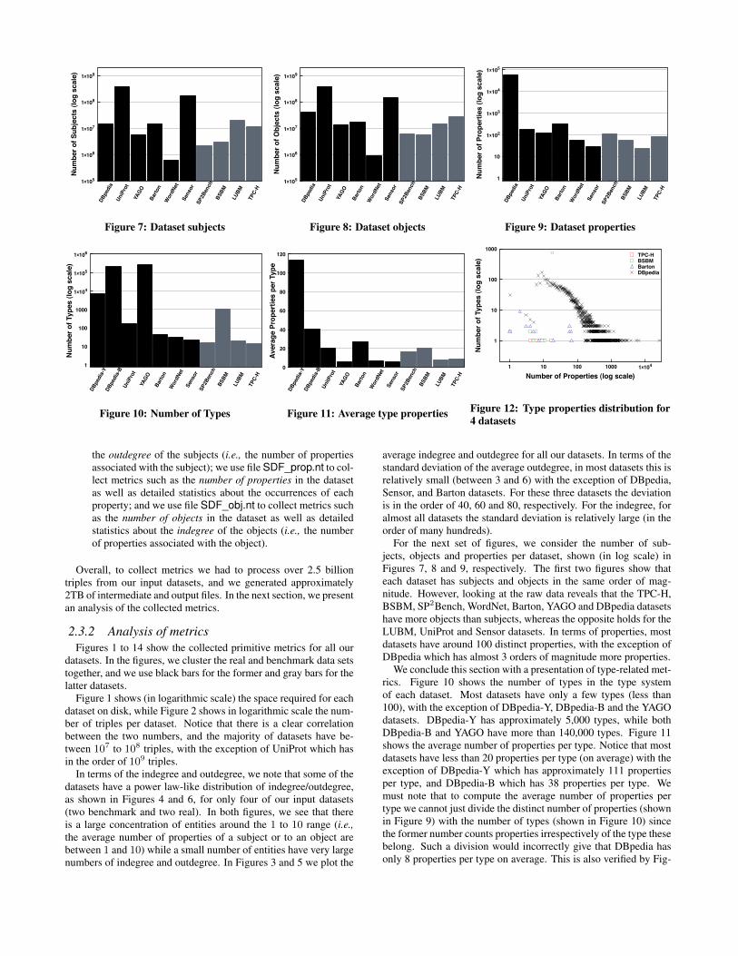
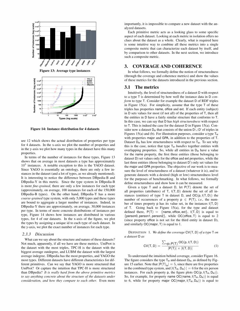
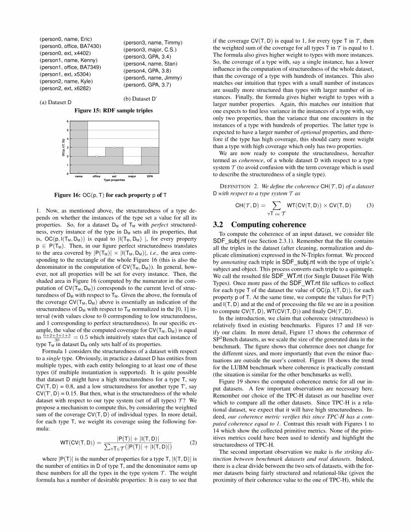
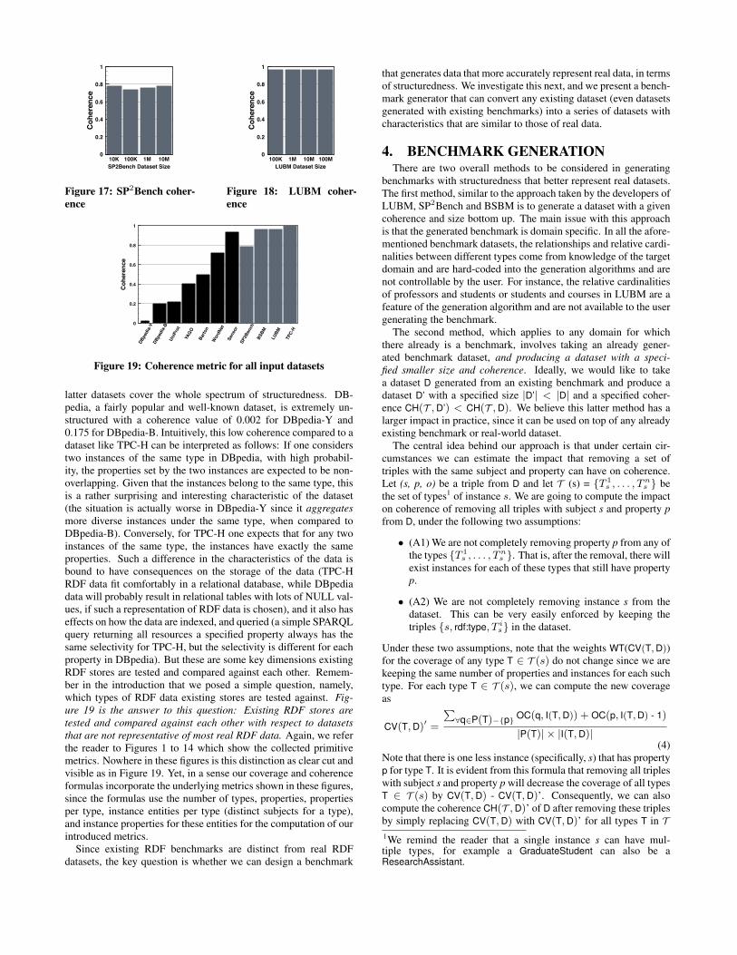
2.3.2 Analysis of metricsFigures 1 to 14 show the collected primitive metrics for all our

datasets. In the figures, we cluster the real and benchmark data setstogether, and we use black bars for the former and gray bars for thelatter datasets.

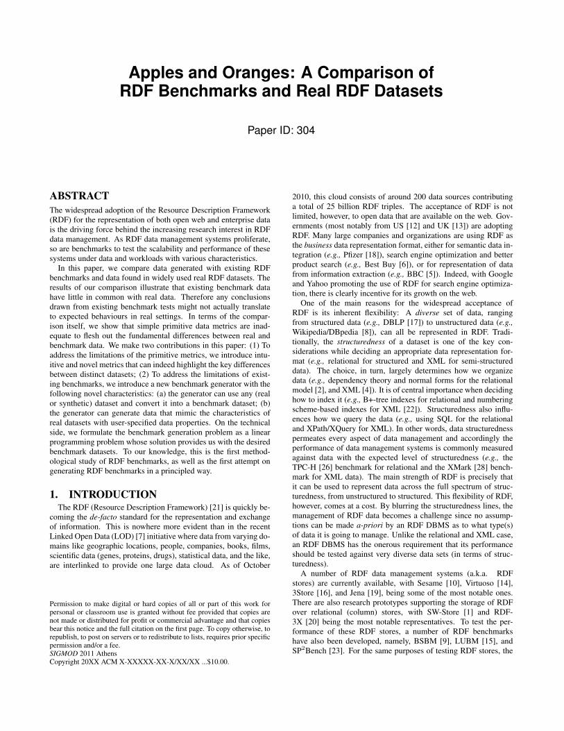
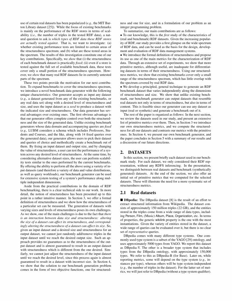
Figure 1 shows (in logarithmic scale) the space required for eachdataset on disk, while Figure 2 shows in logarithmic scale the num-ber of triples per dataset. Notice that there is a clear correlationbetween the two numbers, and the majority of datasets have be-tween 107 to 108 triples, with the exception of UniProt which hasin the order of 109 triples.

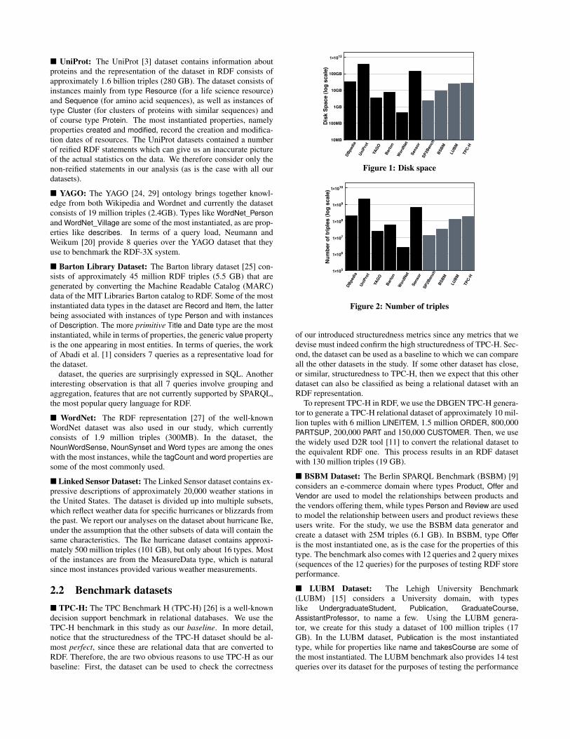
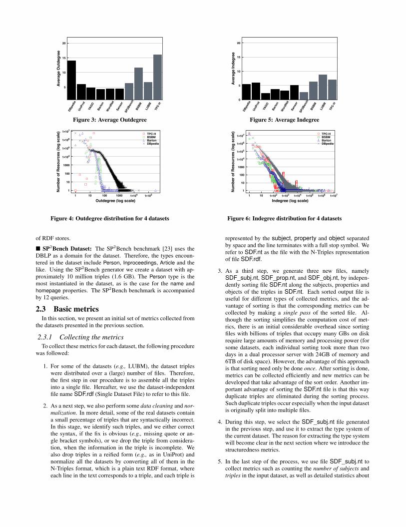
In terms of the indegree and outdegree, we note that some of thedatasets have a power law-like distribution of indegree/outdegree,as shown in Figures 4 and 6, for only four of our input datasets(two benchmark and two real). In both figures, we see that thereis a large concentration of entities around the 1 to 10 range (i.e.,the average number of properties of a subject or to an object arebetween 1 and 10) while a small number of entities have very largenumbers of indegree and outdegree. In Figures 3 and 5 we plot the

average indegree and outdegree for all our datasets. In terms of thestandard deviation of the average outdegree, in most datasets this isrelatively small (between 3 and 6) with the exception of DBpedia,Sensor, and Barton datasets. For these three datasets the deviationis in the order of 40, 60 and 80, respectively. For the indegree, foralmost all datasets the standard deviation is relatively large (in theorder of many hundreds).

For the next set of figures, we consider the number of sub-jects, objects and properties per dataset, shown (in log scale) inFigures 7, 8 and 9, respectively. The first two figures show thateach dataset has subjects and objects in the same order of mag-nitude. However, looking at the raw data reveals that the TPC-H,BSBM, SP2Bench, WordNet, Barton, YAGO and DBpedia datasetshave more objects than subjects, whereas the opposite holds for theLUBM, UniProt and Sensor datasets. In terms of properties, mostdatasets have around 100 distinct properties, with the exception ofDBpedia which has almost 3 orders of magnitude more properties.

We conclude this section with a presentation of type-related met-rics. Figure 10 shows the number of types in the type systemof each dataset. Most datasets have only a few types (less than100), with the exception of DBpedia-Y, DBpedia-B and the YAGOdatasets. DBpedia-Y has approximately 5,000 types, while bothDBpedia-B and YAGO have more than 140,000 types. Figure 11shows the average number of properties per type. Notice that mostdatasets have less than 20 properties per type (on average) with theexception of DBpedia-Y which has approximately 111 propertiesper type, and DBpedia-B which has 38 properties per type. Wemust note that to compute the average number of properties pertype we cannot just divide the distinct number of properties (shownin Figure 9) with the number of types (shown in Figure 10) sincethe former number counts properties irrespectively of the type thesebelong. Such a division would incorrectly give that DBpedia hasonly 8 properties per type on average. This is also verified by Fig-

DBpe

dia-

YDB

pedi

a-B

UniP

rot

YAGO

Barto

nW

ordN

etSe

nsor

SP2B

ench

BSBM

LUBM

TPC-

H

1

10

100

1000

1x104

1x105

1x106

1x107

1x108

Num

ber o

f Ins

tanc

es (l

og s

cale

)

Figure 13: Average type instances

1 10 100 1000 1x104 1x105

Types (log scale)

1

10

100

1000

1x104

1x105

1x106

1x107

1x108

Num

ber o

f Ins

tanc

es (l

og s

cale

) TPC-HBSBMBartonDBpedia

Figure 14: Instance distribution for 4 datasets

ure 12 which shows the actual distribution of properties per typefor 4 datasets. In the x-axis we plot the number of properties andin the y-axis we plot how many types in the dataset have this manyproperties.

In terms of the number of instances for these types, Figure 13shows that on average in most datasets a type has approximately105 instances. A notable exception to this is the YAGO dataset.Since YAGO is essentially an ontology, there are only a few in-stances in the dataset (and a lot of types, as we already mentioned).It is interesting to notice the difference between DBpedia-B andDBpedia-Y in this metric. Since the type system in DBpedia-Bis more fine-grained, there are only a few instances for each type(approximately, on average, 100 instances for each of the 150,000DBpedia-B types). On the other hand, DBpedia-Y has a morecoarse-grained type system, with only 5,000 types and these typesare bound to aggregate a larger number of instances. Indeed, inDBpedia-Y there are approximately, on average, 30,000 instancesper type. In terms of more concrete distributions of instances pertype, Figure 14 shows how instances are distributed in varioustypes, for 4 of our datasets. In the x-axis of the figure, we plotthe types by assigning a unique id to each type of each dataset. Inthe y-axis, we plot the exact number of instances for each type.

2.3.3 DiscussionWhat can we say about the structure and nature of these datasets?

Not much, apparently, if all we have are these metrics. UniProt isthe dataset with the most triples, TPC-H is the dataset with thebiggest average outdegree, and LUBM the dataset with the largestaverage indegree. DBpedia has the most properties, and YAGO themost types. Different datasets have different characteristics for dif-ferent primitives. Can we say that YAGO is more structured thatUniProt? Or capture the intuition that TPC-H is more structuredthan DBpedia? It is really hard from the above primitive metricsto say anything concrete about the structure of the datasets underconsideration, and how they compare to each other. Even more

importantly, it is impossible to compare a new dataset with the an-alyzed datasets.

Each primitive metric acts as a looking glass to some specificaspect of each dataset. Looking at each metric in isolation offers noclues about the dataset as a whole. Clearly, what is required hereis some intuitive way to combine all these metrics into a singlecomposite metric that can characterize each dataset by itself, andby comparison to other datasets. In the next section, we introducesuch a composite metric.

3. COVERAGE AND COHERENCEIn what follows, we formally define the notion of structuredness

(through the coverage and coherence metrics) and show the valuesof these metrics for the datasets introduced in the previous section.

3.1 The metricsIntuitively, the level of structuredness of a dataset D with respect

to a type T is determined by how well the instance data in D con-form to type T. Consider for example the dataset D of RDF triplesin Figure 15(a). For simplicity, assume that the type T of thesetriples has properties name, office and ext. If each entity (subject)in D sets values for most (if not all) of the properties of T, then allthe entities in D have a fairly similar structure that conforms to T.In this case, we can say that D has high structuredness with respectto T. This is indeed the case for the dataset D in Figure 15(a). Con-sider now a dataset DM that consists of the union D∪D’ of triples inFigures 15(a) and (b). For illustration purposes, consider a type TM

with properties major and GPA, in addition to the properties of T.Dataset DM has low structuredness with respect to TM. To see whythis is the case, notice that type TM bundles together entities withoverlapping properties. So, while all entities in DM have a valuefor the name property, the first three entities (those belonging todataset D) set values only for the office and ext properties, while thelast three entities (those belonging to dataset D’) only set values forthe major and GPA properties. The objective of our work is to mea-sure the level of structuredness of a dataset (whatever it is), and togenerate datasets with a desired (high or low) structuredness levelfor the purposes of benchmarking. In what follows, we formallydefine structuredness and show how it can be measured.

Given a type T and a dataset D, let P(T) denote the set ofall properties (attributes) of T, I(T,D) denote the set of all in-stances (entities) of type T in dataset D, and OC(p, I(T,D)) thenumber of occurrences of a property p ∈ P(T), i.e., the num-ber of times property p has its value set, in the instances I(T,D)of T. Going back to Figure 15(a), for the type and datasetdefined there, P(T) = {name, office, ext}, I(T,D) is equal to{person0, person1, person2}, while OC(office, T) is equal to 2(since property office is not set for the third entity in dataset D),and similarly OC(major, T) is equal to 1.

DEFINITION 1. We define the coverage CV(T,D) of a type T ona dataset D as

CV(T,D) =

∑∀p∈P(T) OC(p, I(T,D))

|P(T)| × |I(T,D)| (1)

To understand the intuition behind coverage, consider Figure 16.The figure considers the type TM and dataset DM, as defined by Fig-ure 15 earlier. Note that |P(T)M| = 5, since there are five propertiesin the combined type system, and |I(TM,DM) | = 6 for the six personinstances. For each property p, the figure plots OC(p, I(TM,DM)).So, for example, for property name OC(name, I(TM,DM)) is equalto 6, while for property major OC(major, I(TM,DM)) is equal to

(person0, name, Eric)(person0, office, BA7430)(person0, ext, x4402)(person1, name, Kenny)(person1, office, BA7349)(person1, ext, x5304)(person2, name, Kyle)(person2, ext, x6282)

(a) Dataset D

(person3, name, Timmy)(person3, major, C.S.)(person3, GPA, 3.4)(person4, name, Stan)(person4, GPA, 3.8)(person5, name, Jimmy)(person5, GPA, 3.7)

(b) Dataset D’

Figure 15: RDF sample triples

name office ext major GPAType properties

0

1

2

3

4

5

6

OC

(p, I

(T, D

))

Figure 16: OC(p, T) for each property p of T

1. Now, as mentioned above, the structuredness of a type de-pends on whether the instances of the type set a value for all itsproperties. So, for a dataset DM of TM with perfect structured-ness, every instance of the type in DM sets all its properties, thatis, OC(p, I(TM,DM)) is equal to |I(TM,DM) |, for every propertyp ∈ P(TM). Then, in our figure perfect structuredness translatesto the area covered by |P(TM)| × |I(TM,DM)|, i.e., the area corre-sponding to the rectangle of the whole Figure 16 (this is also thedenominator in the computation of CV(TM,DM)). In general, how-ever, not all properties will be set for every instance. Then, theshaded area in Figure 16 (computed by the numerator in the com-putation of CV(TM,DM)) corresponds to the current level of struc-turedness of DM with respect to TM. Given the above, the formula ofthe coverage CV(TM,DM) above is essentially an indication of thestructuredness of DM with respect to TM normalized in the [0, 1] in-terval (with values close to 0 corresponding to low structuredness,and 1 corresponding to perfect structuredness). In our specific ex-ample, the value of the computed coverage for CV(TM,DM) is equalto 6+2+3+1+3

30= 0.5 which intuitively states that each instance of

type TM in dataset DM only sets half of its properties.Formula 1 considers the structuredness of a dataset with respect

to a single type. Obviously, in practice a dataset D has entities frommultiple types, with each entity belonging to at least one of thesetypes (if multiple instantiation is supported). It is quite possiblethat dataset D might have a high structuredness for a type T, sayCV(T,D) = 0.8, and a low structuredness for another type T’, sayCV(T’,D) = 0.15. But then, what is the structuredness of the wholedataset with respect to our type system (set of all types) T ? Wepropose a mechanism to compute this, by considering the weightedsum of the coverage CV(T,D) of individual types. In more detail,for each type T, we weight its coverage using the following for-mula:

WT(CV(T,D)) =|P(T)|+ |I(T,D)|∑

∀T∈T (|P(T)|+ |I(T,D)|) (2)

where |P(T)| is the number of properties for a type T, |I(T,D)| isthe number of entities in D of type T, and the denominator sums upthese numbers for all the types in the type system T . The weightformula has a number of desirable properties: It is easy to see that

if the coverage CV(T,D) is equal to 1, for every type T in T , thenthe weighted sum of the coverage for all types T in T is equal to 1.The formula also gives higher weight to types with more instances.So, the coverage of a type with, say a single instance, has a lowerinfluence in the computation of structuredness of the whole dataset,than the coverage of a type with hundreds of instances. This alsomatches our intuition that types with a small number of instancesare usually more structured than types with larger number of in-stances. Finally, the formula gives higher weight to types with alarger number properties. Again, this matches our intuition thatone expects to find less variance in the instances of a type with, sayonly two properties, than the variance that one encounters in theinstances of a type with hundreds of properties. The latter type isexpected to have a larger number of optional properties, and there-fore if the type has high coverage, this should carry more weightthan a type with high coverage which only has two properties.

We are now ready to compute the structuredness, hereaftertermed as coherence, of a whole dataset D with respect to a typesystem T (to avoid confusion with the term coverage which is usedto describe the structuredness of a single type).

DEFINITION 2. We define the coherence CH(T ,D) of a datasetD with respect to a type system T as

CH(T ,D) =∑∀T in T

WT(CV(T,D))× CV(T,D) (3)

3.2 Computing coherenceTo compute the coherence of an input dataset, we consider file

SDF_subj.nt (see Section 2.3.1). Remember that the file containsall the triples in the dataset (after cleaning, normalization and du-plicate elimination) expressed in the N-Triples format. We proceedby annotating each triple in SDF_subj.nt with the type of triple’ssubject and object. This process converts each triple to a quintuple.We call the resulted file SDF_WT.nt (for Single Dataset File WithTypes). Once more pass of the SDF_WT.nt file suffices to collectfor each type T of the dataset the value of OC(p, I(T,D)), for eachproperty p of T. At the same time, we compute the values for P(T)and I(T,D) and at the end of processing the file we are in a positionto compute CV(T,D), WT(CV(T,D)) and finaly CH(T ,D).

In the introduction, we claim that coherence (structuredness) isrelatively fixed in existing benchmarks. Figures 17 and 18 ver-ify our claim. In more detail, Figure 17 shows the coherence ofSP2Bench datasets, as we scale the size of the generated data in thebenchmark. The figure shows that coherence does not change forthe different sizes, and more importantly that even the minor fluc-tuations are outside the user’s control. Figure 18 shows the trendfor the LUBM benchmark where coherence is practically constant(the situation is similar for the other benchmarks as well).

Figure 19 shows the computed coherence metric for all our in-put datasets. A few important observations are necessary here.Remember our choice of the TPC-H dataset as our baseline overwhich to compare all the other datasets. Since TPC-H is a rela-tional dataset, we expect that it will have high structuredness. In-deed, our coherence metric verifies this since TPC-H has a com-puted coherence equal to 1. Contrast this result with Figures 1 to14 which show the collected primitive metrics. None of the prim-itives metrics could have been used to identify and highlight thestructuredness of TPC-H.

The second important observation we make is the striking dis-tinction between benchmark datasets and real datasets. Indeed,there is a clear divide between the two sets of datasets, with the for-mer datasets being fairly structured and relational-like (given theproximity of their coherence value to the one of TPC-H), while the

10K 100K 1M 10MSP2Bench Dataset Size

0

0.2

0.4

0.6

0.8

1

Coh

eren

ce

Figure 17: SP2Bench coher-ence

100K 1M 10M 100MLUBM Dataset Size

0

0.2

0.4

0.6

0.8

1

Coh

eren

ce

Figure 18: LUBM coher-ence

DBpedia-Y

DBpedia-B

UniProt

YAGO

Barton

WordNet

Sensor

SP2Bench

BSBM

LUBM

TPC-H

0

0.2

0.4

0.6

0.8

1

Coherence

Figure 19: Coherence metric for all input datasets

latter datasets cover the whole spectrum of structuredness. DB-pedia, a fairly popular and well-known dataset, is extremely un-structured with a coherence value of 0.002 for DBpedia-Y and0.175 for DBpedia-B. Intuitively, this low coherence compared to adataset like TPC-H can be interpreted as follows: If one considerstwo instances of the same type in DBpedia, with high probabil-ity, the properties set by the two instances are expected to be non-overlapping. Given that the instances belong to the same type, thisis a rather surprising and interesting characteristic of the dataset(the situation is actually worse in DBpedia-Y since it aggregatesmore diverse instances under the same type, when compared toDBpedia-B). Conversely, for TPC-H one expects that for any twoinstances of the same type, the instances have exactly the sameproperties. Such a difference in the characteristics of the data isbound to have consequences on the storage of the data (TPC-HRDF data fit comfortably in a relational database, while DBpediadata will probably result in relational tables with lots of NULL val-ues, if such a representation of RDF data is chosen), and it also haseffects on how the data are indexed, and queried (a simple SPARQLquery returning all resources a specified property always has thesame selectivity for TPC-H, but the selectivity is different for eachproperty in DBpedia). But these are some key dimensions existingRDF stores are tested and compared against each other. Remem-ber in the introduction that we posed a simple question, namely,which types of RDF data existing stores are tested against. Fig-ure 19 is the answer to this question: Existing RDF stores aretested and compared against each other with respect to datasetsthat are not representative of most real RDF data. Again, we referthe reader to Figures 1 to 14 which show the collected primitivemetrics. Nowhere in these figures is this distinction as clear cut andvisible as in Figure 19. Yet, in a sense our coverage and coherenceformulas incorporate the underlying metrics shown in these figures,since the formulas use the number of types, properties, propertiesper type, instance entities per type (distinct subjects for a type),and instance properties for these entities for the computation of ourintroduced metrics.

Since existing RDF benchmarks are distinct from real RDFdatasets, the key question is whether we can design a benchmark

that generates data that more accurately represent real data, in termsof structuredness. We investigate this next, and we present a bench-mark generator that can convert any existing dataset (even datasetsgenerated with existing benchmarks) into a series of datasets withcharacteristics that are similar to those of real data.

4. BENCHMARK GENERATIONThere are two overall methods to be considered in generating

benchmarks with structuredness that better represent real datasets.The first method, similar to the approach taken by the developers ofLUBM, SP2Bench and BSBM is to generate a dataset with a givencoherence and size bottom up. The main issue with this approachis that the generated benchmark is domain specific. In all the afore-mentioned benchmark datasets, the relationships and relative cardi-nalities between different types come from knowledge of the targetdomain and are hard-coded into the generation algorithms and arenot controllable by the user. For instance, the relative cardinalitiesof professors and students or students and courses in LUBM are afeature of the generation algorithm and are not available to the usergenerating the benchmark.

The second method, which applies to any domain for whichthere already is a benchmark, involves taking an already gener-ated benchmark dataset, and producing a dataset with a speci-fied smaller size and coherence. Ideally, we would like to takea dataset D generated from an existing benchmark and produce adataset D’ with a specified size |D’| < |D| and a specified coher-ence CH(T ,D’) < CH(T ,D). We believe this latter method has alarger impact in practice, since it can be used on top of any alreadyexisting benchmark or real-world dataset.

The central idea behind our approach is that under certain cir-cumstances we can estimate the impact that removing a set oftriples with the same subject and property can have on coherence.Let (s, p, o) be a triple from D and let T (s) = {T 1

s , . . . , Tns } be

the set of types1 of instance s. We are going to compute the impacton coherence of removing all triples with subject s and property pfrom D, under the following two assumptions:

• (A1) We are not completely removing property p from any ofthe types {T 1

s , . . . , Tns }. That is, after the removal, there will

exist instances for each of these types that still have propertyp.

• (A2) We are not completely removing instance s from thedataset. This can be very easily enforced by keeping thetriples {s, rdf:type, T is} in the dataset.

Under these two assumptions, note that the weights WT(CV(T,D))for the coverage of any type T ∈ T (s) do not change since we arekeeping the same number of properties and instances for each suchtype. For each type T ∈ T (s), we can compute the new coverageas

CV(T,D)′ =

∑∀q∈P(T)−{p} OC(q, I(T,D)) + OC(p, I(T,D) - 1)

|P(T)| × |I(T,D)|(4)

Note that there is one less instance (specifically, s) that has propertyp for type T. It is evident from this formula that removing all tripleswith subject s and property p will decrease the coverage of all typesT ∈ T (s) by CV(T,D) - CV(T,D)’. Consequently, we can alsocompute the coherence CH(T ,D)’ of D after removing these triplesby simply replacing CV(T,D) with CV(T,D)’ for all types T in T1We remind the reader that a single instance s can have mul-tiple types, for example a GraduateStudent can also be aResearchAssistant.

(s). Finally, we compute the impact on the coherence of D of theremoval as:

coin(T (s), p) = CH(T ,D)− CH(T ,D)′

Let us illustrate this process with an example. Consider thedataset DM introduced in Figure 15 and assume we would like toremove the triple (person1, ext, x5304) from DM. Then the newcoverage for the type person in this dataset becomes 6+2+2+1+3

30≈

0.467, hence the impact on the coverage of person is approximately0.5 − 0.467 = 0.033. In this example, DM contains a single type,therefore the coherence of the dataset is the same as the coveragefor person, which brings us to coin({person },ext) ≈ 0.033.

4.1 Benchmark generation algorithmIn this section we outline our algorithm to generate benchmark

datasets of desired coherence and size by taking a dataset D andproducing a dataset D’ ⊂ D such that CH(T ,D) = γ and |D’| = σ,where γ and σ are specified by the user. To do this, we need todetermine which triples need to removed from D to obtain D’. Wewill formulate this as a integer programming problem and solve itusing an existing integer programming solver.

Previously in this section, for a set of types S ⊆ T and a prop-erty p, we have shown how to compute coin(S,p), which representsthe impact on coherence of removing all triples with subjects thatare instances of the types in S and properties equal to p. For sim-plification, we will overload notation and use |coin(S, p)| to denotethe number of subjects that are instances of all the types in S andhave at least one triple with property p, i.e.,

|coin(S, p)| = |{s ∈⋂T∈S

I(T,D)|∃(s, p, v) ∈ D}|

Our objective is to formulate an integer programming problemwhose solutions will tell us how many “coins” (triples with subjectsthat are instances of certain types and with a given property) toremove to achieve the desired coherence γ and size σ. We will useX(S,p) to denote the integer programming variable representing thenumber of coins to remove for each type of coin. In the worst case,the number of such variables (and corresponding coin types) for Dcan be 2τπ, where τ is the number of types in the dataset and πis the number of properties in the dataset. However, in practice,many type combinations will not have any instances – for instance,in LUBM, we will not find instances of UndergraduateStudent thatare also instance of Course or Department. For LUBM, we foundthat although there are 15 types and 18 properties, we only have73 valid combinations (sets of types and property with at least onecoin available).

To achieve the desired coherence, we will formulate the follow-ing constraint and maximization criteria for the integer program-ming problem.∑

S⊆T ,pcoin(S, p)× X(S, p) ≤ CH(T ,D)− γ (C1)

MAXIMIZE∑

S⊆D,pcoin(S, p)× X(S, p) (M)

Inequality C1 states that the amount by which we decrease co-herence (by removing coins) should be less than or equal than theamount we need to remove to get from CH(T ,D) (the coherenceof the original dataset) to γ (the desired coherence). Objectivefunction M states that the amount by which we decrease coher-ence should be maximized. The two elements together ensure thatwe decrease the coherence of D by as much as possible, while notgoing below γ.

We will also put lower and upper bounds on the number of coinsthat can be removed. Remember that assumption (A1) required usnot to remove any properties from any types, so we will ensurethat at least one coin of each type remains. Furthermore, we willenforce assumption (A2) about not removing instances from thedataset by always keeping triples with the rdf:type property.

∀S ⊆ T , p 0 ≤ X(S, p) ≤ |coin(S, p)| − 1 (C2)

Achieving the desired size σ is similar, but requires an approx-imation. Under the simplifying assumption that all properties aresingle-valued (i.e., there is only one triple with a given subject anda given property in D), we could write the following constraint:∑

S⊆T ,p|X(S, p)| = |D| − σ

This equation would ensure that we remove exactly the right num-ber of coins to obtain size σ assuming that all properties are single-valued (meaning one coin represents exactly one triple). However,this assumption does not hold for any of the datasets we have seen.In particular, for LUBM, many properties are multi-valued. As anexample, a student can be enrolled in multiple courses, a paper hasmany authors, etc. We will address this by computing an averagenumber of triples per coin type, which we denote by ct(S,p), andrelaxing the size constraint as follows:

(1− ρ)× (|D| − σ) ≤∑

S⊆T ,pX(S, p)× ct(S, p) (C3)

∑S⊆T ,p

X(S, p)× ct(S, p) ≤ (1 + ρ)× (|D| − σ) (C4)

In these two constraints, ρ is a relaxation parameter. The pres-ence of ρ is required because of the approximation we introducedby using the average number of triples per coin. In practice, set-ting ρ helped us tune the result of our algorithm closer to the targetcoherence and size.

We are now ready to outline the algorithm that generates a bench-mark dataset of desired coherence γ and size σ from an originaldataset D:

• (Step 1) Compute the coherence CH(T ,D) and the coin val-ues coin(S,p) and average triples per coin ct(S,p) for all setsof types S ⊆ T and all properties p.

• (Step 2) Formulate the integer programming problem bywriting constraints C1, C2, C3, C4 and objective functionM. Solve the integer programming problem.

• (Step 3) If the problem did not have a solution, then try tomake the dataset smaller by removing a percentage of in-stances and continue from Step 1.

• (Step 4) If the problem had a solution, then for each coingiven by S and p, remove triples with X(S,p) subjects thatare instances of types in S and have property p.

• (Step 5) If the resulting dataset size is larger than σ, performpost-processing by attempting to remove from triples withthe same subject and property.

We have previously explained in detail how steps (1) and (2) canbe executed. Step (3) is an adjustment in case there is no solution tothe linear programming problem. Remember that assumption (A2)required us not to remove entire instances from the dataset if the in-teger programming formulation is to produce the correct number of

coins to remove. In practice we found that for certain combinationsof γ and σ the integer programming problem does not have solu-tions – in particular for cases where the desired coherence γ is high,but the desired size σ is low (i.e., we have to remove many coins,but we should not decrease coherence much). For these cases, wefound that we can remove entire instances from D first to bringdown its size, then reformulate the integer programming problemand find a solution. The intuition behind this approach is that whenstarting with original datasets of very high coherence (e.g., LUBM,TPC-H, etc.), removing instances uniformly at random will not de-crease coherence much (if at all), since the coverage for all typesis high, but it can decrease dataset size to a point where our integerprogramming approach finds a solution.

To perform this removal of instances effectively, we needed tounderstand how many instances to remove from the original datasetto have a high probability of finding a solution on the new dataset.In our experiments, the integer programming problem always hada solution for σ

|D| ≈γ

CH(T ,D) . Therefore, we want to remove

enough instances as to have the size of our new dataset approx-

imately CH(T ,D)γ

× σ. Assuming that the dataset size is pro-portional to the number of instances2, then we should remove uni-

formly at random a proportion of 1− CH(T ,D)γ

× σ

|D| instances toarrive at a dataset for which we have a good chance of solving theinteger programming problem. After this process, we must restartthe algorithm since the coherence and the numbers of coins for thedataset after the instance removal may be different than those of theoriginal dataset.

In Step (4), we perform the actual removal of triples accordingto the solutions to the integer programming problem. Step (5) isa post-processing step that attempts to compensate for the approx-imation introduced by constraints C3 and C4 of the integer pro-gramming problem. Specifically, if the solution we obtain afterStep (4) has a size higher than σ, then we can compensate by look-ing at triples with the same subject and property. Note that basedon the way we have defined coverage for types, the formula mea-sures whether instances have at least one value for each propertyof that type. Therefore, if a property is multi-valued, we can safelyremove the triples containing extra values (ensuring that we keep atleast one value), and therefore reduce the size of the dataset. Whilethis step is optional, it can improve the match between σ and theactual size of the resulting dataset.

Note that the algorithm presented in this section performs at leasttwo passes through the original dataset D. The first pass is per-formed in Step (1) to compute coherence and coin values and theaverage number of triples per coin. The second pass is performedin Step (4), where coins are removed from D to generate the de-sired dataset. If the integer programming problem does not have asolution, then at least four passes are required: one pass in Step (1),one pass in Step (3) to remove instances, a third pass in Step (1)to compute coherence and coin values after instance removal andfinally a fourth pass in Step (4) to remove coins from the dataset.In addition, in either case there may be an additional pass over theresulting dataset to adjust for size (Step 5).

Our discussion of future work in Section 5 includes a query eval-uation study that looks at how coherence of a dataset affects queryperformance. To perform such a study, we will need datasets withthe same size but varying coherence and a set of queries that re-turn the same results for each dataset. In our implementation, weadded an additional option of specifying a list of triples that shouldnot be removed from a dataset. This option impacts Step (2) where

2We found this to be true for all datasets we examined.

we need impose different upper bounds on the X(S,p) (to accountfor coins that cannot be removed) and in Step (4), to avoid remov-ing the “forbidden” triples. The following process helps obtain thenecessary datasets for a query evaluation study:

1. Start with a dataset D of high coherence and size.

2. Generate a first dataset D0 with the desired size σ and thesame coherence as D by removing entire instances uniformlyat random.

3. Issue queries over D0 and record all triples required to pro-duce answers to these queries.

4. Generate datasets D1, . . . , Dn of different coherence and thesame size σ using the benchmark generation algorithm pre-sented here. Use the set of triples computed in the previousstep as “forbidden” triples during the generation to ensurethat all datasets yield the same answers to all queries.

By experimenting with the option of avoiding triples, we found thatit works well for queries of medium to high selectivity. Queries oflow selectivity require many triples to answer, thus greatly dimin-ishing the set of useful coins that can reduce coherence of a dataset.

4.2 Experimental results and discussionWe implemented our benchmark generation algorithm in Java

and performed experiments on multiple original datasets, bothbenchmark and real-world. We used lpsolve 5.53 as our integerprogramming solver with a timeout of 100 seconds per problem.We report results from running the benchmark generation on fourservers with identical configuration: 2 dual-core 3GHz processors,24GB of memory and 12 TB of shared disk space. We used thesemachines to run experiments in parallel, but we also performedsimilar experiments (one at a time) on a standard T7700 2.4 Ghz3GB of RAM laptop machine.

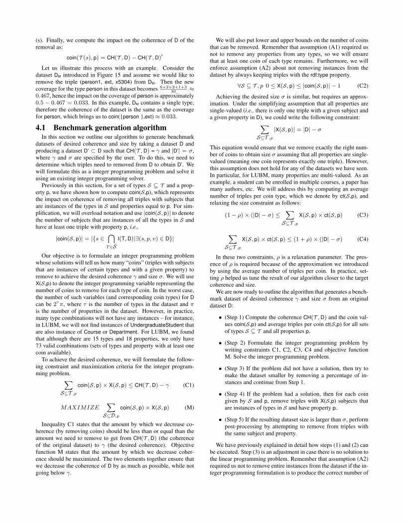
We started with the LUBM dataset in different sizes (100Ktriples, 1, 10 and 100 million triples). For each, we exe-cuted benchmark generation with nine sets of parameters, γ ∈{0.25, 0.5, 0.75} and σ ∈ {0.25, 0.5, 0.75} × |D|. The resultsare shown in Figures 20–23. In each figure, the x axis representsthe percentage of the original dataset size desired and the y axisrepresents the coherence desired (as an absolute value, not as a per-centage of original coherence). The square markers in each figurerepresent the ideal output and the X markers represent the achievedsize/coherence combination. We can easily see that with the ex-ception of the 75% size, 0.25 coherence combination the algorithmachieves almost perfect matches. The relaxation parameter ρ wasset to a default of 0.1 for all LUBM runs.

The 75% size, 0.25 coherence combination essentially requiresthat we lower coherence by a large margin (remember that the orig-inal coherence of LUBM is above 0.9), while maintaining most ofthe triples in the dataset. In this case, the integer programmingsolver maximizes the amount of coherence that can be removed (asinstructed by the objective function), but cannot achieve perfect co-herence. This is caused by the fact that we have an upper bound onthe amount by which coherence should decrease (constraint C1),but no lower bound like we do for size. However, we noticed thatby introducing a lower bound for the amount by which coherencecan decrease has two downsides: (i) it introduces a new controlparameter (in addition to ρ) and (ii) without adjustment of this pa-rameter, the integer programming solver either times out or cannotsolve the problem in many cases. As a result, we decided that the3http://lpsolve.sourceforge.net/5.5/

0% 25% 50% 75% 100%Percentage of initial dataset size

0

0.25

0.50

0.75

1

Coh

eren

ceTarget Size/Coherence for 100K LUBM triplesAchieved Size/Coherence for 100K LUBM triples

Figure 20: LUBM 100K

0% 25% 50% 75% 100%Percentage of initial dataset size

0

0.25

0.50

0.75

1

Coh

eren

ce

Target Size/Coherence for 1M LUBM triplesAchieved Size/Coherence for 1M LUBM triples

Figure 21: LUBM 1M

0% 25% 50% 75% 100%Percentage of initial dataset size

0

0.25

0.50

0.75

1

Coh

eren

ce

Target Size/Coherence for 10M LUBM triplesAchieved Size/Coherence for 10M LUBM triples

Figure 22: LUBM 10M

0% 25% 50% 75% 100%Percentage of initial dataset size

0

0.25

0.50

0.75

1

Coh

eren

ce

Target Size/Coherence for 100M LUBM triplesAchieved Size/Coherence for 100M LUBM triples

Figure 23: LUBM 100M

100K 1M 10M 100MLUBM Dataset Size

1

10

100

1000

10000

Avg

Gen

erat

ion

time

(sec

s)

Figure 24: Running time: LUBM

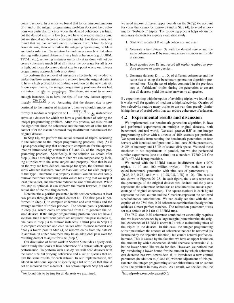
0% 25% 50% 75% 100%Percentage of initial dataset size

0

0.25

0.50

0.75

Coh

eren

ce

Target Size/Coherence for SP2Bench triplesAchieved Size/Coherence for SP2Bench triples

Figure 25: SP2Bench

0% 25% 50% 75% 100%Percentage of initial dataset size

0

0.25

0.50

0.75

1

Coh

eren

ce

Target Size/Coherence for TPC-H triplesAchieved Size/Coherence for TPC-H triples

Figure 26: TPC-H

0% 25% 50% 75% 100%Percentage of initial dataset size

0

0.25

0.50

0.75

Coh

eren

ce

Target Size/Coherence for WordNet triplesAchieved Size/Coherence for WordNet triples

Figure 27: Wordnet

algorithm is more useful without the lower bound on coherence re-duction (which means an upperbound on resulting coherence). Asan alternative, in cases where such combinations are desired, theuser can start with a larger dataset size – for instance, instead ofstarting with a 1 million triple dataset requiring 75% size and 0.25coherence, the user can start with a 3 million triple dataset and re-quest 25% size and 0.25 coherence.

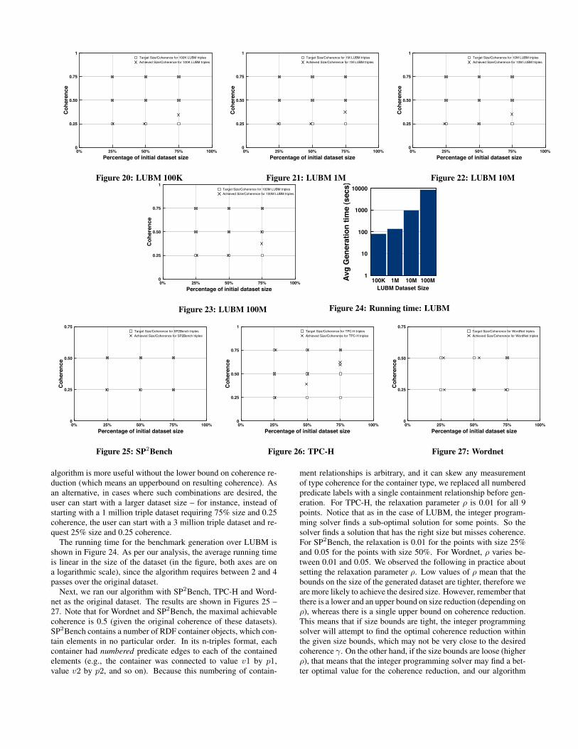
The running time for the benchmark generation over LUBM isshown in Figure 24. As per our analysis, the average running timeis linear in the size of the dataset (in the figure, both axes are ona logarithmic scale), since the algorithm requires between 2 and 4passes over the original dataset.

Next, we ran our algorithm with SP2Bench, TPC-H and Word-net as the original dataset. The results are shown in Figures 25 –27. Note that for Wordnet and SP2Bench, the maximal achievablecoherence is 0.5 (given the original coherence of these datasets).SP2Bench contains a number of RDF container objects, which con-tain elements in no particular order. In its n-triples format, eachcontainer had numbered predicate edges to each of the containedelements (e.g., the container was connected to value v1 by p1,value v2 by p2, and so on). Because this numbering of contain-

ment relationships is arbitrary, and it can skew any measurementof type coherence for the container type, we replaced all numberedpredicate labels with a single containment relationship before gen-eration. For TPC-H, the relaxation parameter ρ is 0.01 for all 9points. Notice that as in the case of LUBM, the integer program-ming solver finds a sub-optimal solution for some points. So thesolver finds a solution that has the right size but misses coherence.For SP2Bench, the relaxation is 0.01 for the points with size 25%and 0.05 for the points with size 50%. For Wordnet, ρ varies be-tween 0.01 and 0.05. We observed the following in practice aboutsetting the relaxation parameter ρ. Low values of ρ mean that thebounds on the size of the generated dataset are tighter, therefore weare more likely to achieve the desired size. However, remember thatthere is a lower and an upper bound on size reduction (depending onρ), whereas there is a single upper bound on coherence reduction.This means that if size bounds are tight, the integer programmingsolver will attempt to find the optimal coherence reduction withinthe given size bounds, which may not be very close to the desiredcoherence γ. On the other hand, if the size bounds are loose (higherρ), that means that the integer programming solver may find a bet-ter optimal value for the coherence reduction, and our algorithm

can still approach the desired size using the compensation in Step(5). Generally, choosing ρ depends on the original dataset size andthe desired dataset size. For small initial datasets, having “loose”bounds (i.e., ρ = 0.1) is a good option because it gives the integerprogramming solver a larger solution space to work for. For largerdatasets, we do not want too much flexibility in the size, hence wecan choose low relaxation values (i.e., 0.01 in TPC-H). However,if the target dataset size is also large (75% of the original), we canagain have higher values of the relaxation parameter because westill achieve a good match.

5. CONCLUSIONSIn this paper, we presented an extensive study of the character-

istics of real and benchmark RDF data. Through this study, weillustrated that primitive metrics, although useful, offer little in-sight about the inherent characteristics of datasets and how thesecompare to each other. We introduced a macroscopic metric, calledcoherence, that essentially combines many of these primitive met-rics and is used to measure the structuredness of different datasets.We showed that while real datasets cover the whole structurednessspectrum, benchmark datasets are very limited in their structured-ness and are mostly relational-like. Since structuredness plays animportant role on how we store, index and query data, the aboveresult indicates that existing benchmarks do not accurately predictthe behaviour of RDF stores in realistic scenarios. In response tothis limitation, we also introduced a benchmark generator whichcan be used to generate benchmark datasets that actually resemblereal datasets in terms of structuredness, size, and content. This isfeasible since our generator can use any dataset as input (real orsynthetic) and generate a benchmark out of it. On the technicalside, we formally introduced structuredness through the coherencemetric, and we showed how the challenge of benchmark genera-tion can be solved by formulating it as an integer programmingproblem.

Using this work as a starting point, there are several avenues weare investigating next. Specifically, one important topic is the ef-fects of structuredness on RDF storage strategies. Our preliminaryinvestigation shows that while relational column stores are consid-ered a popular and effective storage strategy for RDF data, this as-sumption holds true mainly for data with high structuredness. Suchdata often exhibit a small number of types in their type system, andeach type has a small number of properties. Then, a column storeapproach to RDF requires only a few tens of tables in the RDBMS.However, data with low structuredness, like DBpedia or Yago, havelarge number of types and properties (in the thousands). For suchdatasets, a column store solution would require thousands of tablesin RDBMS and is thus not expected to scale.

Another avenue we are investigating relates to the indexing andquerying of RDF data. Structuredness influences both the type andthe density of the indexes used. At the same time, it influences theselectivity of queries and therefore the overall query performance.We are planning to investigate the concrete effects of structurednesson query performance and contrast again the performance of equiv-alent queries over datasets with varying structuredness. Ideally, forthis comparison to be meaningful, the queries should return iden-tical results across all varying structuredness datasets. We alreadyhave done some preliminary work to this end, and included an ex-clusion list in our integer programming formulation so as to ex-clude certain triples (those that participate in the query result) fromremoval, as we compute a new dataset with smaller structuredness.It turns out however, that trying to maintain such triples for low-selectivity queries often leads to a linear programming problem thatis impossible to solve. Therefore, we are considering other alter-

natives to meaningfully compare low-selectivity queries across thedifferent datasets.

6. REFERENCES[1] D. J. Abadi, A. Marcus, S. R. Madden, and K. Hollenbach. Scalable

semantic web data management using vertical partitioning. In VLDB,pages 411–422. VLDB Endowment, 2007.

[2] S. Abiteboul, R. Hull, and V. Vianu. Foundations of Databases.Addison-Wesley, 1995.

[3] R. Apweiler, A. Bairoch, C. H. Wu, W. C. Barker, B. Boeckmann,S. Ferro, E. Gasteiger, H. Huang, R. Lopez, M. Magrane, M. J.Martin, D. A. Natale, C. O’Donovan, N. Redaschi, and L. S. Yeh.Uniprot: the universal protein knowledgebase. Nucleic Acids Res.,32:D115–D119, 2004.

[4] M. Arenas and L. Libkin. A normal form for xml documents. InPODS, pages 85–96, 2002.

[5] BBC World Cup 2010 dynamic semantic publishing.http://www.bbc.co.uk/blogs/bbcinternet/2010/07/bbc_world_cup_2010_dynamic_sem.html.

[6] Best Buy jump starts data web marketing.http://www.chiefmartec.com/2009/12/best-buy-jump-starts-data-web-marketing.html.

[7] C. Bizer, T. Heath, and T. Berners-Lee. Linked data - the story so far.Int. J. Semantic Web Inf. Syst., 5(3):1–22, 2009.

[8] C. Bizer, J. Lehmann, G. Kobilarov, S. Auer, C. Becker, R. Cyganiak,and S. Hellmann. DBpedia—a crystallization point for the web ofdata. Web Semantics, 7(3):154–165, 2009.

[9] C. Bizer and A. Schultz. The berlin sparql benchmark. Int. J.Semantic Web Inf. Syst., 5(2):1–24, 2009.

[10] J. Broekstra, A. Kampman, and F. van Harmelen. Sesame: A genericarchitecture for storing and querying rdf and rdf schema. InInternational Semantic Web Conference, pages 54–68, 2002.

[11] D2R Server: Publishing Relational Databases on the Semantic Web.http://www4.wiwiss.fu-berlin.de/bizer/d2r-server/.

[12] Data.gov. http://www.data.gov/.[13] Data.gov.uk. http://www.data.gov.uk/.[14] O. Erling and I. Mikhailov. Rdf support in the virtuoso dbms. In

CSSW, pages 59–68, 2007.[15] Y. Guo, Z. Pan, and J. Heflin. Lubm: A benchmark for owl

knowledge base systems. J. Web Semantics, 3(2-3):158–182, 2005.[16] S. Harris and N. Gibbins. 3store: Efficient bulk rdf storage. In PSSS,

2003.[17] L3S Research Center D2R Server publishing the DBLP Bibliography

Database. http://dblp.l3s.de/d2r/.[18] Making a Semantic Web Business Case at Pfizer. http:

//www.semanticweb.com/news/making_a_semantic_web_business_case_at_pfizer_161731.asp.

[19] B. McBride. Jena: Implementing the rdf model and syntaxspecification. In SemWeb, 2001.

[20] T. Neumann and G. Weikum. Rdf-3x: a risc-style engine for rdf.PVLDB, 1(1):647–659, 2008.

[21] Resource Description Framework (RDF).http://www.w3.org/RDF/.

[22] V. Sans and D. Laurent. Prefix based numbering schemes for xml:techniques, applications and performances. Proc. VLDB Endow.,1(2):1564–1573, 2008.

[23] M. Schmidt, T. Hornung, G. Lausen, and C. Pinkel. Sp2bench: Asparql performance benchmark. In ICDE, pages 222–233, 2009.

[24] F. M. Suchanek, G. Kasneci, and G. Weikum. Yago: A large ontologyfrom wikipedia and wordnet. J. Web Sem., 6(3):203–217, 2008.

[25] The MIT Barton Library dataset.http://simile.mit.edu/rdf-test-data/.

[26] The TPC Benchmark H. http://www.tpc.org/tpch.[27] WordNet: A lexical database for English (WordNet RDF/OWL

Files). http://www.w3.org/2006/03/wn/wn20/.[28] XMark: An XML Benchmark Project.

http://www.xml-benchmark.org/.[29] YAGO: Yet Another Great Ontology.

http://www.mpi-inf.mpg.de/yago-naga/yago/.