AppendixH

8/3/2019 AppendixH

http://slidepdf.com/reader/full/appendixh 1/79

H APPENDIX

CEUS SSC MODEL HAZARD INPUT DOCUMENT (HID)

H.1 Introduction

This appendix describes the CEUS SSC Model in the main report. The purpose of this document is

to provide the necessary information so that an analyst experienced in PSHA can implement the

seismic source model. The appendix contains the logic tree structure and descriptions of the parameters that define the frequency and spatial distribution of potential future earthquakes. The

reader is referred to the main report for detailed descriptions of methods and rationale used to

develop the model parameters. The digital files that contain the input parameters described in thisappendix are contained on the project website. The area covered by this model is shown on Figure

H-1-1 along with the locations of the test sites used for hazard sensitivity calculations presented in

Chapter 8.

H.2 Seismic Source Model Structure and Master Logic Tree

The structure of the CEUS SSC model is described in Section 4. The CEUS SSC Model contains

two general types of seismic sources. The first type of seismic source uses the recorded history of seismicity to model the frequency and spatial distribution of moderate to large earthquakes (M ≥ 5).

These sources are denoted as distributed seismicity sources. They cover the entire region shown on

Figure H-1-1. The second type of seismic source uses the paleo-earthquake record to model thefrequency and spatial distribution of repeated large magnitude earthquakes (RLMEs) at specific

locations.

Figure H-2-1 shows the master logic tree for the CEUS SSC model. The basis for this logic tree is

described in Section 4.2. The first node addresses the conceptual approach used to characterize thedistributed seismicity sources. Two approaches are used. The first is an approach in which

distributed seismicity is modeled using seismicity rates that smoothly vary across the entire study

region. The study region is subdivided only on the basis of differences in maximum magnitudes.

The first branch is designated as the Mmax Zones approach. The second approach uses seismicsource zones defined on a seismotectonic basis to model distributed seismicity. The second branch

is designated as the Seismotectonic Zones approach. In both approaches specific seismic sources are

used to model individual sources of RLMEs. The RLME sources represent additional sources of seismic hazard that are added to the hazard from the distributed seismicity sources.

The models developed for the various types of seismic sources are described in subsequent sections

of this appendix.

H-1

8/3/2019 AppendixH


Appendix H

H.3 Mmax Zones Distributed Seismicity Sources

Figure H-3-1 shows the logic tree structure to be used for the distributed seismicity sources on the

Mmax Zones branch of the master logic tree. This logic tree is discussed in Section 4.2.3 of the

main report.

H.3.1 Division of Study Region

The first node addresses whether or not the study region is divided into two zones that havedifferent Mmax distributions. If “No” then the entire study region, shown on Figure H-1-1, is

treated as a single source. If “Yes” then the study region is divided into Mesozoic and younger

extended regions (MESE) and those regions that do not display such evidence (NMESE).

H.3.2 Location of Boundary of Mesozoic Extension

The second node of the Mmax Zones logic tree, which applies only to the Mesozoic and younger

separation branch, addresses the alternative boundaries between the MESE and NMSES regions.

Two alternatives are used. The first, labeled the “Wide Interpretation” has a broad interpretation of the extent of Mesozoic extension. Figure H-3-2 shows the location of this boundary. The second,

labeled the “Narrow Interpretation” makes a narrow interpretation of the extent of Mesozoic

extension. Figure H3-3 shows the location of this boundary.

H.3.3 Magnitude Interval Weights for Fitting Earthquake Occurrence Parameters

The third node addresses the issue of the weight assigned to smaller magnitudes in the estimation of seismicity parameters for the seismic source zones. Three cases are used, Cases A, B, and E. The

weights assigned to individual magnitude intervals are discussed in Section 5.3.2.2.

H.3.4 Mmax Zones

The next element of the Mmax Zones logic tree (which is not a node but a listing) identifies the

Mmax zone designations for each case. The vertical bar without a dot at the branching pointdesignates the addition of hazard from all of the listed sources, as opposed to weighted alternatives

that appear with a dot on the logic tree. The coordinates defining the boundaries of the Mmax Zonesare contained in the file Source_Zones_Geometry.zip on the project web site. The boundary for

each zone is contained in an ASCII file named for the source with the extension “zon” (e.g.

“MESE-N.zon” for the MESE-N Mmax zone).

H.3.5 Seismogenic Crustal Thickness

The fifth node of the logic tree represents the uncertainty distribution for seismogenic crustal

thickness. The distribution used for each Mmax zone is listed in Table H-3-1. These are epistemicuncertainties representing weighted alternative assessments of the seismogenic crustal thickness for

each Mmax zone.

H-2

8/3/2019 AppendixH


Appendix H

H.3.6 Future Earthquake Rupture Characteristics

The sixth node addresses the uncertainty distributions for the rupture characteristics of future

earthquakes. In the CEUS SSC model a single aleatory distribution is applied to each Mmax zone.

These aleatory distributions are listed in Table H-3-2.

The area of individual earthquake ruptures is modeled using the relationship:

log10(A in km2) =M – 4.366 (H-1)

The rupture aspect ratio is 1:1 until the rupture reaches maximum rupture width. For larger rupturesthe width is fixed and the length is increased to obtain the area given by Equation H-1. This model

is used for all earthquake sources described in this HID.

H.3.7 Assessment of Seismicity Rates

The seventh node of the Mmax Zones logic tree on Figure H-3-1 addresses the approach used for

assessing seismicity rates and their spatial distribution. Allowing both the a-value and the b-value to

vary spatially is the selected approach. The approach is described in Section 5.3.2. Seismicity parameters are estimated for ½° longitude by ½° latitude cells or partial cells.

H.3.8 Degree of Smoothing Applied in Defining Spatial Smoothing of Seismicity Rates

The eighth node of the logic tree addresses the degree of smoothing applied in the seismicity

parameter estimation in each source region. A single approach, the “Objective” approach, is used to

select the degree of smoothing. This is discussed in Section 5.3.2.2 of the main report.

H.3.9 Uncertainty in Earthquake Recurrence Rates

The ninth node of the logic tree addresses the epistemic uncertainty in earthquake recurrence parameters. The recurrence parameter distributions are represented by eight alternative spatialdistributions developed from the fitted parameter distributions. These alternatives are described in

Section 5.3.2. The result is eight equally weighted alternative sets of recurrence parameters for each

Mmax Zone. The recurrence parameters are contained in the file “CEUS_SSC_All_xyab_Files.zip”on the project web site. The recurrence parameters are contained in ASCII files for each Mmax zone

using the following file naming convention.

Zone_Case_Realization.ext

The “Zone” portion of the file name is the Mmax Zone name, MESE-W, MESE-N, NMESE-W,

NMESE-N, and STUDY_R for the case when the entire study region is considered a single Mmax

Zone. The “Case” portion of the file name refers to Case A, Case B, or Case E on Figure H-4. The“ Realization” portion of the file name takes on the values “01”, “02”, “03”, “04”, “05”, “06”, “07”,and “08” to indicate the eight equally weighted alternative sets of recurrence parameters. The “ext ”

portion of the file name takes on two values. An extension of “ xyab” indicates a file containingrecurrence parameters for PSHA calculations that integrate over magnitude starting from a

minimum magnitude, m0, of M 5.0. An extension of “ xyab4” indicates a file containing recurrence

parameters for PSHA calculations that integrate over magnitude starting from a minimum

H-3

8/3/2019 AppendixH


Appendix H

magnitude, m0, of M 4.0, which would typically be used for PSHA calculations incorporating the

Cumulative Absolute Velocity (CAV) filter.

Each recurrence parameter file contains a header with the case description. The second record

provides the number of individual cells and the nominal cell size in degrees (e.g 0.5 for ½°

longitude by ½° latitude cells). The remaining records contain the following information in fivecolumns:

Longitude and latitude of the center of the cell or partial cell, in degrees.

Recurrence rate of earthquakes of magnitude m0 and larger per equatorial degrees2. For thefiles with extension “ xyab” this is the rate of M 5 and larger earthquakes and for files with

extension “ xyab4” this is the rate of M 4 and larger earthquakes.

Beta value. This is the b-value expressed in natural log units { β = b x ln(10)}.

Area of the cell in equatorial degrees2. The absolute value of recurrence rate is the product

of the values in the third and fifth columns.

H.3.10 Uncertainty in Maximum Magnitude

The tenth node of the logic tree addresses the uncertainty in the maximum magnitude for each

Mmax Zone. These epistemic distributions are listed in Table H-3-3.

H.4 Seismotectonic Zones

Figure H-4-1 shows the logic tree structure for the seismotectonic source zones component of themaster logic tree. The components of the source model logic tree are described below. Table H-4-1

lists the seismotectonic source zones.

H.4.1 Alternative Zonation Models

The first two nodes address the alternative zonation models. The first node addresses the uncertainty

in the western boundary of the Paleozoic Extended Crust seismotectonic zone. The two alternatives

are the narrow interpretation (0.8) and the wide interpretation (0.2). The second node of the logictree addresses the uncertainty in the eastern extent of the Reelfoot Rift zone (RR) —whether or not

it includes the Rough Creek Graben (RCG). These two logic tree levels lead to the four alternative

seismotectonic zonation configurations shown on Figures H-4-2 through H-4-5. The discussion of

this assessment and the associated weights is given in Section 7.3.6.3 of the main report. As shownon Figures H-4-1 though H-4-5, the alternative zonation models produce alternative versions of the

Mid-Continent source zone. These are designated MidC-A, MidC-B, MidC-C, and MidC-D.

H.4.2 Magnitude Interval Weights for Fitting Earthquake Occurrence Parameters

The third node addresses the issue of the weight assigned to smaller magnitudes in the estimation of

seismicity parameters for the seismic source zones. As in the Mmax Zones model, three cases are

used, Cases A, B, and E. The weights assigned to individual magnitude intervals are discussed in

Section 5.3.2.2.

H-4

8/3/2019 AppendixH


Appendix H

H.4.3 Seismotectonic Zones

The next element of the logic tree is again a listing of the individual seismotectonic source zones for

each zonation model. The vertical bar without a dot at the branching point designates the addition of

hazard from all of the listed sources. The coordinates defining the boundaries of the source are

contained in the file Source_Zones_Geometry.zip on the project web site. The boundary for eachzone is contained in an ASCII file named for the source with the extension “zon” (e.g. “AHEX.zon”

for the AHEX seismotectonic source zone).

H.4.4 Seismogenic Crustal Thickness

The fifth node of the logic tree represents the uncertainty distribution for seismogenic crustal

thickness. The distribution used for each seismotectonic zone is listed in Table H-4-2. These are

epistemic uncertainties representing weighted alternatives.

H.4.5 Future Earthquake Rupture Characteristics

The sixth node addresses the uncertainty distributions for the rupture characteristics of futureearthquakes. In the CEUS SSC model a single aleatory distribution is applied to each

seismotectonic zone. These aleatory distributions are listed in Table H-4-3.

The area of individual earthquake ruptures is modeled using the relationship given in Equation H-1

above. The rupture aspect ratio is 1:1 until the rupture reaches maximum rupture width. For larger ruptures the width is fixed and the length is increased to obtain the area given by Equation H-1. This

model is used for all earthquake sources described in this HID.

H.4.6 Assessment of Seismicity Rates

The seventh node of the logic tree on Figure H-4-1 addresses the approach used for assessing

seismicity rates and their spatial distribution. Allowing both the a-value and the b-value to varyspatially is the selected approach. The approach is described in Section 5.3.2. Seismicity parameters

are estimated for ¼° longitude by ¼° latitude cells or partial cells for all sources except the Mid-

Continent sources, for which the cell size ½° longitude by ½° latitude is used.

H.4.7 Degree of Smoothing Applied in Defining Spatial Smoothing of Seismicity Rates

The eighth node of the logic tree addresses the degree of smoothing applied in the seismicity

parameter estimation in each source region. A single approach is used to select the degree of smoothing for each source. This is discussed in Section 5.3.2.2 of the main report. For all sources

but the St. Lawrence Rift zone (SLR) the “Objective” approach is used.

H.4.8 Uncertainty in Earthquake Recurrence Rates

The ninth node of the logic tree addresses the epistemic uncertainty in earthquake recurrence parameters. As was the case for the Mmax zones, the recurrence parameter distributions are

represented by eight alternative spatial distributions developed from the fitted parameter

distributions. These alternatives are described in Section 5.3.2. The result is eight equally weightedalternative sets of recurrence parameters for each Seismotectonic Zone. The recurrence parameters

H-5

8/3/2019 AppendixH


Appendix H

are contained in the file “CEUS_SSC_All_xyab_Files.zip” on the project web site. The recurrence

parameters are contained in ASCII files for each seismotectonic zone using the naming convention

and file format described in Section H.3.9.

H.4.9 Uncertainty in Maximum Magnitude

The tenth node of the logic tree addresses the uncertainty in the maximum magnitude for each

seismotectonic zone. These distributions are listed in Table H-4-4.

H.5 RLME Sources

This section describes the models for the RLME sources. As shown on Figure H-2-1, these sourcesare considered to be additional sources superimposed on the distributed seismicity sources on the

seismotectonic branch of the master logic tree or on the Mmax Zones on the Mmax Zone branch of

the master logic tree. Figure H-5-1 shows the overall structure of the RLME sources model. There

are 10 RLME sources. Each source has a logic tree defining the uncertainty in characterization.Discussion of the each of the individual RLME sources is contained in Section H.5 of the main

report. The locations of the RLME sources are shown on Figure H-5-2. The parameters for each of the RLME sources present in the following sections are contained in files located on the CEUS SSC

Project website in the RLME directory.

H.5.1 Charlevoix RLME Seismic Source Model

The Charlevoix RLME source is described in Section 6.1.1 of the main text. The logic tree for theCharlevoix RLME source is shown on Figure H-5.1-1. The parameters are located on the CEUS

SSC Project web site in the file “Charlevoix_RLME.xls.”

H.5.1.1 Temporal Clustering

The first node of the logic tree addresses the issue of temporal clustering of earthquakes in the present tectonic stress regime. This node of the logic tree is not applicable to the Charlevoix RLME

source.

H.5.1.2 Localizing Tectonic Features

Because the occurrence of RLMEs in the Charlevoix zone cannot be associated with a specific

feature, future RLMEs are modeled as occurring randomly within the RLME source zone, as

indicated on the second node of the logic tree (Figure H-5.1-1).

H.5.1.3 Geometry and Style of Faulting

The geometry of the Charlevoix RLME source is shown on Figure H-5.1-2. A single source zonegeometry is used. The coordinates are contained on the “Geometry” tab of the file

“Charlevoix_RLME.xls.” Given the small source size and uncertain fault locations, the boundaries

of the Charlevoix RLME source are leaky, allowing ruptures to extend beyond the source boundary

by 50 percent.

The thickness of seismogenic crust is modeled with equal weight on 25 and 30 km (16 and 19 mi.),

as shown on the fourth node of the logic tree (Figure H-5.1-1).

H-6

8/3/2019 AppendixH


Appendix H

Future earthquake ruptures are modeled as reverse faulting earthquakes. Rupture geometry is

modeled by a single aleatory distribution as shown by the fifth node of the logic tree. Strikes of

ruptures are to be uniformly distributed over azimuths of 0 to 360 degrees. Fault dips are uniformly

distributed between 45 and 60 degrees.

H.5.1.4 RLME Magnitude

Table H-5.1-1 lists the epistemic uncertainty distribution for the expected magnitude of futureearthquakes associated with the Charlevoix RLME source. Aleatory variability in the size of an

individual Charlevoix RLME is modeled as a uniform distribution of ±0.25M units centered on the

expected RLME magnitude value listed in Table H-5.1-1.

H.5.1.5 RLME Recurrence

The remaining nodes of the Charlevoix RLME logic tree address uncertainties in the specification

of the annual frequency of RLMEs.

Recurrence Methods and Data

Two approaches are used to assess RLME recurrence. The “Earthquake Recurrence Intervals”

approach is assigned a weight of 0.2. This approach leads to data set 1. The “Earthquake Count in aTime Interval” approach is assigned a weight of 0.8. There are two data sets associated with this

branch. Data set 2 is assigned a conditional weight of 0.75 and data set 3 is assigned a conditional

weight of 0.25.

Earthquake Recurrence Model

The Poisson model is used as the earthquake recurrence model, with a weight of 1.0.

RLME Annual Frequency

The final node of the logic tree addresses the uncertainty distributions for the annual frequency of

RLMEs. These distributions are listed in Tables H-5.1-2, H-5.1-3, and H-5.1-4. The data are

contained in the file “Charlevoix_RLME.xls.”

H.5.2 Charleston RLME Seismic Source Model

Charleston RLME source is described in Section 6.1.2 of the main text. Figure H-5.2-1 shows the

logic tree for the Charleston RLME source. The parameters are located on the CEUS SSC Project

web site in the file “Charleston_RLME.xls.”


The first node of the logic tree (Figure H-5.2-1) addresses the issue of temporal clustering of earthquakes on the Charleston RLME source. The Charleston RLME seismic source is modeled as

“in” a temporal cluster with a weight of 0.9 and “out” of a temporal cluster with a weight of 0.1. For

the “in” branch, the remaining portion of the logic tree is used to define the hazard from this source.

On the “out” branch the Charleston RLME source is not included in calculation of the total seismic

hazard.

H-7

8/3/2019 AppendixH


Appendix H

H.5.2.2 Localizing Feature

The second node of the Charleston RLME source logic tree indicates whether future earthquakes in

the Charleston seismic zone will be associated with a specific localizing tectonic feature. The

approach used for this source is to model future ruptures to occur randomly with the source.


The third node of the Charleston RLME source logic tree addresses the alternative geometries of the

parameters Charleston RLME source. Three alternative source zone geometries are included in themodel. These are shown on Figure H-5.2-2. The coordinates of the three source geometries are

given in the file “Charleston_RLME.xls.”

The fourth node of the logic tree indicates the three values of seismogenic crustal thickness used for

all source geometries.

The geometries and style of faulting for the three source geometries are specified as follows.

Charleston Local source configuration: Future ruptures are oriented northeast, parallel to thelong axis of the zone. Ruptures are modeled as occurring on vertical strike-slip faults. All boundaries of the Charleston Local source are strict, such that ruptures are not allowed to

extend beyond the zone boundaries.

Charleston Narrow source configuration: Future ruptures are oriented north-northeast,

parallel to the long axis of the zone. Ruptures are modeled as occurring on vertical strike-slip faults. The northeast and southwest boundaries of the Charleston Narrow source are

leaky, whereas the northwest and southeast boundaries of the Charleston Narrow source are

strict.

Charleston Regional source configuration: Future rupture orientations are represented by

two alternatives: (1) future ruptures oriented parallel to the long axis of the source(northeast) with 0.80 weight, and (2) future ruptures oriented parallel to the short axis of thesource (northwest) with 0.20 weight. In both cases, future ruptures are modeled as occurring

on vertical strike-slip faults. All boundaries of the Charleston Regional source are strict.


The sixth node of the Charleston RLME source logic tree defines the magnitude of future large

earthquakes in the Charleston RLME source. The RLME magnitude distribution is given inTable H-5.2-1. Aleatory variability in the size of an individual Charleston RLME is modeled as a

uniform distribution of ±0.25M units centered on the expected RLME magnitude value.


The remaining nodes of the Charleston RLME source logic tree address the uncertainty in modeling

of the recurrence rare of Charleston RLMEs.

Recurrence Method

The recurrence data for the Charleston RLME source consists of ages of past RLMEs estimated

from the paleoliquefaction record. Therefore, node seven of the logic tree indicates that recurrence

H-8

8/3/2019 AppendixH


Appendix H

for the Charleston RLME source is based solely on the “Earthquake Recurrence Intervals”

approach.

Time Period

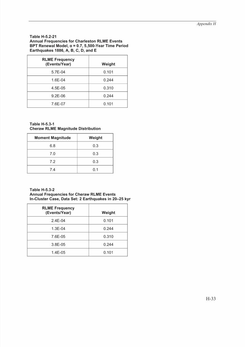
The eighth node of the Charleston RLME source logic tree assesses length and completeness of the paleoliquefaction record. Two alternatives are considered: the approximately 2,000-year record of

Charleston earthquakes with 0.80 weight and the approximately 5,500-year record with 0.20 weight.

Earthquake Count

The ninth node of the Charleston logic tree addresses the uncertainty in the number of RLMEs that

have occurred in the Charleston RLME source. For the 2,000-year record, a single model is used.

For the 5.500-year, three alternatives are used as shown on Figure H-5.2-1.


The tenth node of the Charleston RLME source logic tree defines the earthquake recurrence models

used for the regional, local, and narrow source zones (Figure H-5.2-1). For the regional and localsources, only the Poisson model is used. For the more “fault-like” narrow source zone, the Poisson

model is assigned 0.90 weight, and the BPT renewal model is assigned 0.10 weight. Use of the BPT

renewal model requires specification of the coefficient of variation of the repeat time for RLMEs, parameter α. The uncertainty distribution for α is shown on the eleventh node of the Charleston

RLME source logic tree.


The final (twelfth) node of the logic tree addresses the uncertainty distributions for the annual

frequency of RLMEs. There are 20 uncertainty distributions corresponding to the various

approaches and data sets defined in Levels 8, 9, 10, and 11 of the logic tree. These are given inTables H-5.2 -2 through H-5.2-21. Tables H-5.2-2 through H-5.2-6 provide the recurrence ratedistributions for the Poisson Occurrence model and Tables H-5.2-7 through H-5.2-21 provide the

recurrence rate distributions for the BPT Renewal model. Figure H-5.2-1 shows the relationship

between the branches of the logic tree and the recurrence rate distribution tables.

H.5.3 Cheraw RLME Seismic Source Model

The Cheraw RLME source is described in Section 6.1.3 of the main report. Figure H-5.3-1 showsthe logic tree for the Cheraw RLME source. The parameters are located on the CEUS SSC Project

web site in the file “Cheraw_RLME.xls.”


The first node of the logic tree (Figure H-5.3-1) addresses the issue of temporal clustering of earthquakes in the present tectonic stress regime. The within-cluster branch of the logic tree is

assigned a weight of 0.9, and the out-of-cluster branch is assigned a weight of 0.1. These two

branches lead to different recurrence rates

H-9

8/3/2019 AppendixH


Appendix H


The Cheraw RLME source is modeled as a single fault source.


Two alternative lengths are used for the Cheraw RLME source. These are shown on Figure H-5.3-2.The mapped length is assigned a weight of 0.8 and the extended length is assigned a weight of 0.2.

The coordinates for these two geometries are provided in the file “Cheraw_RLME.xls.”

The fourth node of the logic tree provides the uncertainty distribution for the thickness of

seismogenic crust. The generic distribution of 13 km (weight of 0.4), 17 km (weight of 0.4), and 22

km (weight of 0.2) is used.

The fifth node of the logic tree addresses the uncertainty in the dip of the fault. The assigned

uncertainty distribution is: 50°NW (0.6), 65°NW (0.4).

The style of faulting is assessed to be normal. Future ruptures are to be confined to the modeled

fault surface.


The magnitude distribution for the Cheraw RLME source is given in Table H-5.3-1. Aleatory

variability in the size of an individual Cheraw RLME is modeled as a uniform distribution of ±0.25

M units centered on the expected RLME magnitude value.


The remaining nodes of the Cheraw RLME logic tree address the uncertainties in modeling the

recurrence rate of Cheraw RLMEs

Recurrence Method

Two types of data are used for assessing the recurrence frequency of Cheraw RLMEs. The first isthe average slip rate of the fault and the second is the number and timing of previous RLMEs,

allowing application of the “Earthquake Recurrence Intervals” approach. These two approaches are

assigned equal weights.

Recurrence Data

Two data sets are used for the assessment of the in-cluster recurrence rate of Cheraw RLMEs basedon the “Earthquake Recurrence Intervals” approach. The first is the occurrence of two earthquakes

in 20-25 ka, with a weight of 0.4, and the second in the occurrence of three earthquakes in 20-25 ka,

with a weight of 0.6. The total slip of the fault in the range of 3.2 to 4.1 m in 20-25 ka is used to

assess the in-cluster slip rate.

The out-of-cluster recurrence rates for the “Earthquake Recurrence Intervals” approach are based onestimates of the time between in-cluster periods. Out-of-cluster slip rate is based on 7–8 m of offset

in a time period ranging from 400 ka to 2 Ma.

H-10

8/3/2019 AppendixH


Appendix H


The Poisson model is used as the earthquake recurrence model with weight 1.0 for the Cheraw

RLME source.

RLME Annual Frequency The assessed RLME recurrence frequencies for the various data sets are given in Tables H-5.3-2

through H-5.3-6. Figure H-5.3-1 shows the relationship between the branches of the logic tree and

the recurrence rate distribution tables.

H.5.4 Meers RLME Seismic Source Model

The Meers RLME source is described in Section 6.1.4 of the main report. The source logic tree is

shown on Figure H-5.4-1. The data for the Meers RLME is located on the CEUS SSC Project web

site contained in file “Meers_RLME.xls.”


The first node of the logic tree (Figure H-5.4-1) addresses the issue of temporal clustering. The in-cluster branch of the logic tree is given a weight of 0.8 and the out-of-cluster branch a weight of 0.2.

These two alternatives affect both the recurrence rate of the RLMEs and their spatial distribution.


The second branch of the logic tree (Figure H-5.4-1) defined whether future earthquakes associated

with the Meers RLME source are localized along the Meers fault scarp ( designated “Fault” on the

logic tree), or whether they may occur along other structures within the Oklahoma aulacogen(“Random in Zone” on the logic tree). For the in-cluster case, the “Fault” model is used and RLMEs

are constrained to occur on the Meers fault. For the out-of-cluster case, RLMEs the two alternatives

are the “Fault” model and the “Random in Zone” model.


The third through fifth branches of the logic tree describe the source geometry and style of faulting

(Figure H-5.4-1).

The alternative geometries for the “Fault” model consists of the mapped Quaternary trace of theMeers fault (weight 0.9) and an extended fault trace (weight 0.1). These two geometries are shown

on Figure H-5.4-2.

For the “Random-in-Zone” model, the RLMEs are modeled as occurring uniformly distributed

within the boundary of the OKA seismic source zone, also shown on Figure H-5.4-2.

The seismogenic thickness for the Meers RLME source is modeled as either 15 km or 20 km with

equal weights.

For the “Fault” model, future earthquake ruptures are to be modeled as either oblique earthquakes

on a vertical fault (weight 0.5) or reverse-oblique earthquakes dipping 40 degrees southwest.

Ruptures are confined to the model fault surface.

H-11

8/3/2019 AppendixH


Appendix H

For the “Random-in-Zone” model future ruptures are to be modeled as having a N60W strike and a

random dip in the range of 90 to 40 degrees southwest.


The sixth branch of the logic tree describes the earthquake magnitudes for the Meers RLME. TheRLME magnitude distribution is given in Table H-5.4-1. Aleatory variability in the size of an

individual Meers RLME is modeled as a uniform distribution of ±0.25 M units centered on the

expected RLME magnitude value.


The remaining branches of the logic tree define the uncertainty distributions for RLME recurrence

rates.

Recurrence Method

The “Earthquake Recurrence Intervals” approach is used with weight 1.0 (Figure H-5.4-1).

Recurrence Data

The data used to assess the in-cluster recurrence rates consists of two earthquakes in 2.1 to 3 ka.The data used to assess the out-of-cluster case consist of the estimated time between clusters of

activity on the fault.


The Poisson model is used as the earthquake recurrence model with weight 1.0 for the Meers

RLME source.


The final node of the logic tree addresses the uncertainty distributions for the annual frequency of RLMEs (Figure H-5.4-1). These distributions are provided in Tables H-5.4-2 for the in-cluster case

and Table H-5.4-3 for the out-of-cluster case. Note that the out-of-cluster model combined with the

“Random-in-Zone” model for the spatial distribution is assigned the in-cluster recurrence rate

distribution.

H.5.5 New Madrid Fault System RLME Seismic Source Model

The New Madrid Fault System (NMFS) RLME is discussed in Section 6.1.5 of the main report.Figure H-5.5-1 shows the logic tree for this source. The data for this source is on the CEUS SSC

Project web site contained in file “NMFS_RLME.xls.”


The first node of the logic tree (Figure H-5.5-1) addresses the issue of temporal clustering. Three

alternatives are modeled.

With weight 0.9 the NMFS RLME is modeled as being in-cluster.

H-12

8/3/2019 AppendixH


Appendix H

With weight 0.05 the RLME is modeled as being out-of-cluster with no earthquake activity

occurring on the source.

With weight 0.05, the RLME is modeled as being out-of-cluster with a long term rate

assigned to only the Reelfoot Thrust (described below).


The RLMEs associated with the NMFS are modeled as occurring on three fault sources: (1) the

New Madrid South (NMS) fault; (2) the New Madrid North (NMN) fault; and (3) the Reelfoot

Thrust (RFT).


Each of the NMFS fault sources has two alternative geometries as shown on Figures H-5.5-2, H-

5.5-3, and H-5.5-4, respectively. Future NMFS RLMEs are confined to occur on these modeled

faults.

The seismogenic crustal thickness is modeled as being 13 km (weight of 0.3), 15 km (weight of 0.5), or 17 km (weight of 0.2).

The style of faulting for each of the fault sources is based on geologic and seismologic observations.

The NMS fault is modeled as a vertical right-lateral strike-slip fault. The RFT fault is modeled as areverse fault dipping an average of 40 degrees southwest. The NMN fault is modeled as a vertical

right-lateral strike-slip fault.


The magnitudes of RLMEs for the NMFS are assigned in terms of a joint distribution.

Table H-5.5-1 lists the assigned distribution of rupture sets. Aleatory variability in the size of an

individual RLME is modeled as a uniform distribution of ±0.25 M units centered on the expectedRLME magnitude value for each fault source.


The remaining nodes of the NMFS RLME source logic tree address the assessment of earthquake

recurrence rates.

Recurrence Method


Recurrence Data

In-cluster case recurrence rates are based on the 1811-1812, 1450 AD, and 900 AD sequences. Out-

of-cluster recurrence rates for the NMFS are based on timing between clusters.

H-13

8/3/2019 AppendixH


Appendix H


The Poisson and renewal recurrence models are assigned weights of 0.75 and 0.25, respectively, for

the in-cluster case. For the renewal model the BPT model is used with a distribution for the

parameter α shown on the twelfth node of the source logic tree.



RLMEs (Figure H-5.5-1). These distributions are contained in Table H-5.5-2 for the in-cluster Poisson case, Tables H-5.5-3, H-5.5-4, and H-5.5-5 for the in-cluster renewal model cases, and in

Table H-5.5-5 for the out-of-cluster Poisson case.

For the in-cluster case, RLMEs are to be modeled as occurring on all three of the fault sources

within a close period of time (e.g. similar to the 1811-1812 earthquake sequence).

H.5.6 Eastern Rift Margin Fault RLME Seismic Source Model

The Eastern Rift Margin (ERM) fault RLME sources are described in Section 6.1.6 in the main text.The source consists of southern and northern segments. Figure H-5.6-1 shows the logic tree for the

southern segment, ERM-S and Figure H-5.6-2 shows the logic tree for the northern segmentERM-N. The data for these two sources are contained on the CEUS SSC Project web site in files

“ERM-S_RLME.xls” and “ERM-N_RLME.xls.”


The first node of the logic trees addresses the issue of temporal clustering of earthquakes in the

present tectonic stress regime. This node of the logic tree is not applicable to the ERM-S and

ERM-N RLME sources.


The ERM-S and ERM-N RLME sources are modeled as narrow zones. Figures H-5.6-3 and H-5.6-4show the geometries of the sources. Earthquakes are modeled as uniformly distributed in the source

zones.


There are two alternative geometries for the ERM-S RLME source: ERM-SCC (weight of 0.6) and

the ERM-SRP (weight 0.4). These are shown on Figure H-5.6-3. A single geometry is specified for

the ERM-N RLME source.

The probability distribution used to model seismogenic thickness for the ERM-S and ERM-NRLME sources is: 13 km (weight of 0.3), 15 km (weight of 0.5), and 17 km (weight of 0.2).

Future ruptures are to be modeled as vertical strike slip ruptures aligned parallel with the long axis

to the RLME source zones. Both the northeastern and southwestern ends of the zones are modeled

as leaky to allow for uncertainty in the extent of possible reactivated faults along the rift margin.

H-14

8/3/2019 AppendixH


Appendix H


Tables H-5.6-1 and H-5.6-2 list the RLME magnitude distributions for the ERM-S and ERM-N

RLMEs, respectively. Aleatory variability in the size of an RLME is modeled as a uniform

distribution of ±0.25M units centered on the expected RLME magnitude value given in the tables.


The remaining nodes of the ERM-S and ERM-N logic trees address the estimation of recurrence

rate of RLMEs.

Recurrence Method

The “Earthquake Count in a Time Interval” approach is used to assess RLME recurrence frequency

for both the ERM-S and ERM-N sources.

Recurrence Data

For the ERM-S source, three alternative data sets are used to assess RLME recurrence rates: either two, three, or four earthquakes in a 17.7 to 21.7 ka period. The three alternatives have equal weight.

For the ERM-N source, two alternative data sets are use: either one (weight 0.9) or two (weight 0.1)

earthquakes in a 12–35 ka period.


The Poisson model is used as the default earthquake recurrence model with weight 1.0 for both the

ERM-S and ERM-N sources.


Tables H-5.6-3, H-5.6-4, and H-5.6-5 list the distribution of RLME recurrence frequencies for theERM-S source. Tables H-5.6-6 and H-5.6-7 list the distribution of RLME recurrence frequencies

for the ERM-N source.

H.5.7 Marianna Zone RLME Seismic Source Model

The Marianna Zone RLME is described in Section 6.1.7 of the main report. The logic tree for this

source is shown on Figure H-5.7-1. The data for this source is contained on the CEUS SSC Project

web site in file “Marianna_RLME.xls.”


The first node of the logic tree for the RLME source (Figure H-5.7-1) addresses the issue of temporal clustering of earthquakes. The in-cluster model is assigned a weight of 0.5 and the out-of-cluster model is assigned a weight of 0.5. For the “in” branch, the remaining portion of the logic

tree is used to define the hazard from this source. On the “out” branch the Marianna RLME source

is not included in calculation of the total seismic hazard.

H-15

8/3/2019 AppendixH


Appendix H


RLMEs are modeled as occurring randomly with the boundary of the Marianna zone shown on

Figure H-5.7-2.

H.5.7.3 Geometry and Style of FaultingA single geometry for the Marianna RLME source is used. The geometry is shown on

Figure H-5.7-2.

The probability distribution used to model seismogenic thickness is 13 km (weight of 0.3), 15 km

(weight of 0.5), or 17 km (weight of 0.2).

Two equally weighted alternatives for future ruptures of RLMEs are modeled: either vertical strike-

slip ruptures oriented northeast parallel to the sides of the Marianna zone or vertical strike-slip

ruptures oriented northwest parallel to the sides of the Marianna zone. All boundaries to the MAR

zone are leaky.


The distribution for RLME magnitude for the Marianna RLME source is given in Table H-5.7-1.

Aleatory variability in the size of an RLME is modeled as a uniform distribution of ±0.25M units

centered on the expected RLME magnitude value given in the table.


The remaining branches of the logic tree describe the assessment of RLME recurrence rates.

Recurrence Method


Recurrence Data

The two equally weighted data sets consist of either three or four earthquakes with the oldest

occurring approximately 9.9 ka.


The Poisson model is used as the default earthquake recurrence model with weight 1.0 for the

Marianna RLME source.



RLMEs. These distributions are given in Tables H-5.7-2 and H-5.7-3.

H.5.8 Commerce Fault RLME Seismic Source Model

The Commerce RLME source is described in Section 6.1.8 of the main text. The source logic tree is

shown on Figure H-5.8-1. The data for this source is contained on the CEUS SSC Project web site

in file “Commerce_RLME.xls.”

H-16

8/3/2019 AppendixH


Appendix H


This node of the logic tree is not applicable to this source.


RLMEs are modeled as occurring randomly with the boundary of the Commerce zone shown onFigure H-5.8-2.


A single geometry for the Commerce RLME source is modeled.

The uncertainty distribution for seismogenic crustal thickness is: 13 km (weight of 0.3), 15 km

(weight of 0.5), or 17 km (weight of 0.2).

The Commerce RLME source is modeled as a zone of vertical strike-slip faulting. Ruptures are to

be oriented N47°E, subparallel to the Commerce zone boundary. The northeast and southwest

boundaries of the zone are considered leaky boundaries.


Table H-5.8-1 lists the uncertainty distribution for the Commerce RLME magnitude. Aleatoryvariability in the size of an RLME is modeled as a uniform distribution of ±0.25M units centered

on the expected RLME magnitude value given in the table.



Recurrence Method The “Earthquake Recurrence Intervals” approach is used with weight 1.0 (Figure H-5.8-1).

Recurrence Data

The preferred interpretation (weight 0.75) is that two earthquakes have occurred in the past 23 kyr

with the possibility (weight 0.25) that the count is three earthquakes.


The Poisson model is used as the earthquake recurrence model with weight 1.0 for the Commerce

RLME source.


Tables H-5.8-2 and H-5.8-3 list the alternative distributions for RLME frequency for the Commerce

RLME source.

H-17

8/3/2019 AppendixH


Appendix H

H.5.9 Wabash Valley RLME Seismic Source Model

The Wabash Valley RLME source is described in Section 6.1.9 of the main text. The source logic

tree is shown on Figure H-5.9-1. The data for this source is contained on the CEUS SSC Project

web site in file “Wabash_RLME.xls.”


This node of the logic tree is not applicable to this source.


RLMEs are modeled as occurring randomly with the boundary of the Wabash Valley zone shown

on Figure H-5.9-2.


A single zone geometry is used to model the Wabash Valley RLME. This geometry is shown on

Figure H-5.9-2.

Two alternative estimates of the seismogenic thickness of the crust in the Wabash Valley RLME are

used: 17 km (weight of 0.7) or 22 km (weight of 0.3).

The boundaries of the Wabash Valley RLME source zone are modeled as leaky. Earthquakes are to

be modeled with a random strike (uniform 0º to 360º azimuth). The earthquakes are a mixture of 2/3

vertical strike-slip and 1/3 reverse (random dip in the range of 40º to 60º)


Table H-5.9-1 lists the uncertainty distribution for the magnitude of Wabash Valley RLMEs.

Aleatory variability in the size of an RLME is modeled as a uniform distribution of ±0.25M

unitscentered on the expected RLME magnitude value given in the table.



Recurrence Method


Recurrence Data

The available data for characterizing the recurrence rate of Wabash Valley RLMEs are theestimated ages for the Vincennes-Bridgeport and Skelton paleoearthquakes.


The Poisson model is used as the earthquake recurrence model with weight 1.0 for the Wabash

Valley RLME source.

H-18

8/3/2019 AppendixH


Appendix H



RLMEs. This distribution is listed in Table H-5.9-2.

H-19

8/3/2019 AppendixH


Appendix H

Table H-3-1Weighted Alternative Seismogenic Crustal Thickness Values for Mmax Zones

Mmax Zone Crustal Thickness and [Weight]

Study Region 13 km [0.4], 17 km [0.4], 22 km [0.2]

MESE-W 13 km [0.4], 17 km [0.4], 22 km [0.2]

MESE-N 13 km [0.4], 17 km [0.4], 22 km [0.2]

NMESE-W 13 km [0.4], 17 km [0.4], 22 km [0.2]

NMESE-N 13 km [0.4], 17 km [0.4], 22 km [0.2]

Table H-3-2Aleatory Distributions for Characterization of Future Earthquake Ruptures for Mmax Zones

Mmax Zone

SourceBoundary

Characteristics

Sense of Slip(Relative

Frequency)

Rupture Strike(Relative

Frequency)

Rupture Dip(Relative

Frequency)

Study Region,MESE-N,MESE-W,NMESE-N,NMESE-W

Leakya

Strike-slip (2/3)

N50W (0.2)N00E (0.2)N35E (0.4)N60E (0.1)N90E (0.1)

Uniformlydistributed 60º to90º, equally likelydip direction

Reverse (1/3)

N50W (0.2)N00E (0.2)N35E (0.4)

N60E (0.1)N90E (0.1)

Uniformlydistributed 30º to60º, equally likely

dip direction

aLeaky boundary denotes the case were earthquake ruptures are centered on the earthquake epicenter, the

epicenters are contained within the source boundary, but the rupture is allowed to extend beyond the sourceboundary.

Table H-3-3Maximum Magnitude Distributions for Mmax Distributed Seismicity Sources

Weight Assignedto Mmax

Maximum Magnitude for:

StudyRegion MESE_N NMESE_N MESE_W NMESE_W

0.101 6.5 6.4 6.4 6.5 5.7

0.244 6.9 6.8 6.8 6.9 6.1

0.310 7.2 7.2 7.1 7.3 6.6

0.244 7.7 7.7 7.5 7.7 7.2

0.101 8.1 8.1 8.0 8.1 7.9

H-20

8/3/2019 AppendixH


8/3/2019 AppendixH


Appendix H

Table H-4-3Aleatory Distributions for Characterization of Future Earthquake Ruptures for SeismotectonicZones

SeismotectonicZone

Source

BoundaryCharacteristics

Sense of Slip

(RelativeFrequency)

Rupture Strike

(RelativeFrequency)

Rupture Dip

(RelativeFrequency)

AHEX, ECC-AM,MidC-A, MidC-B,MidC-C, MidC-D,PEZ-N, PEZ-W

Leakya

Strike-slip (2/3)

N50W (0.2)N00E (0.2)N35E (0.4)N60E (0.1)N90E (0.1)


Reverse (1/3)

N50W (0.2)N00E (0.2)N35E (0.4)N60E (0.1)N90E (0.1)


ECC-GC, GHEX Leakya

Strike-slip (2/3) Uniform 0º to 180º


Reverse (1/3) Uniform 0º to 180º


GMH Leakya

Strike-slip (0.2)N40W (0.4)N20E (0.4)N90E (0.1)

Uniformlydistributed 60º to90º, equally likely

dip direction

Reverse (0.8)N40W (0.4)N20E (0.4)N90E (0.1)


IBEB Leakya

Reverse Oblique(0.1)

N20W (1.0)75ºE (0.5)75ºW (0.5)

Reverse (0.3) N00E (1.0)

40ºE (0.2)40ºW (0.2)75ºE (0.3)75ºW (0.3)

Strike-slip (0.6)N50W (0.167)N90E (0.333)N40E (0.5)

90º (1.0)

NAP Leakya

Strike-slip (1/3)

N50W (0.2)N00E (0.2)N35E (0.4)N60E (0.1)N90E (0.1)


H-22

8/3/2019 AppendixH


Appendix H

SeismotectonicZone

SourceBoundary

Characteristics

Sense of Slip(Relative

Frequency)

Rupture Strike(Relative

Frequency)

Rupture Dip(Relative

Frequency)

Reverse (2/3)

N50W (0.2)N00E (0.2)

N35E (0.4)N60E (0.1)N90E (0.1)

Uniformly

distributed 30º to60º, equally likelydip direction

OKA Leakya Reverse Oblique

(1.0)Parallel to Long Axis of Zone (1.0)

Uniform 45ºN to75ºN (0.5)Uniform 45ºS to75ºS (0.5)

RR, RR-RCG Leakya

Reverse (0.35) N10W (1.0)

40ºE (0.25)40ºW (0.25)70ºE (0.25)70ºE (0.25)

Strike-slip (0.65)

N50W (0.3)N30E (0.3)N55E (0.3)N90E (0.1)

90º (1.0)

SLR Leakya

Strike-slip (1/3)

N25E (0.2)

N40E (0.2)

N70E (0.2)

N50W (0.15)

N70W (0.15)

NS (0.05)

EW (0.05)


Reverse (2/3)

N25E (0.2)

N40E (0.2)

N70E (0.2)

N50W (0.15)

N70W (0.15)

NS (0.05)

EW (0.05)


aLeaky boundary denotes the case were earthquake ruptures are centered on the earthquake epicenter, the

epicenters are contained within the source boundary, but the rupture is allowed to extend beyond the source

boundary.

H-23

8/3/2019 AppendixH


8/3/2019 AppendixH


Appendix H

Table H-5.1-1Charlevoix RLME Magnitude Distribution

Moment Magnitude Weight

6.75 0.2

7.0 0.5

7.25 0.2

7.5 0.1

Table H-5.1-2Annual Frequencies for Charlevoix RLME EventsData Set 1: 1870 and 1663

RLME Frequency(Events/Year) Weight

9.3E-03 0.101

6.7E-03 0.244

4.2E-03 0.310

2.2E-03 0.244

7.7E-04 0.101

Table H-5.1-3Annual Frequencies for Charlevoix RLME EventsData Set 2: 3 Earthquakes in 6 –7 kyr BP


1.3E-03 0.101

8.4E-04 0.244

5.7E-04 0.310

3.7E-04 0.244

1.9E-04 0.101

H-25

8/3/2019 AppendixH


Appendix H

Table H-5.1-4Annual Frequencies for Charlevoix RLME EventsData Set 3: 4 Earthquakes in 9.5 –10.2 kyr BP


9.8E-04 0.101

6.7E-04 0.244

4.7E-04 0.310

3.2E-04 0.244

1.8E-04 0.101

Table H-5.2-1

Charleston RLME Magnitude Distribution


6.7 0.10

6.9 0.25

7.1 0.30

7.3 0.25

7.5 0.10

Table H-5.2-2Annual Frequencies for Charleston RLME EventsPoisson Model, 2,000-Year Time PeriodEarthquakes 1886, A, B, and C


4.7E-03 0.101

3.1E-03 0.244

2.1E-03 0.310

1.3E-03 0.244

6.8E-04 0.101

H-26

8/3/2019 AppendixH


Appendix H

Table H-5.2-3Annual Frequencies for Charleston RLME EventsPoisson Model, 5,500-Year Time PeriodEarthquakes 1886, A, B, and C

RLME Frequency

(Events/Year) Weight

4.7E-03 0.101

3.1E-03 0.244

2.1E-03 0.310

1.3E-03 0.244

6.8E-04 0.101

Table H-5.2-4Annual Frequencies for Charleston RLME EventsPoisson Model, 5,500-Year Time PeriodEarthquakes 1886, A, B, C, and D


2.7E-03 0.101

1.9E-03 0.244

1.3E-03 0.310

8.8E-04 0.2445.0E-04 0.101

Table H-5.2-5Annual Frequencies for Charleston RLME EventsPoisson Model, 5,500-Year Time PeriodEarthquakes 1886, A, B, C, and E


1.9E-03 0.101

1.3E-03 0.244

9.2E-04 0.310

6.4E-04 0.244

3.4E-04 0.101

H-27

8/3/2019 AppendixH


Appendix H

Table H-5.2-6Annual Frequencies for Charleston RLME EventsPoisson Model, 5,500-Year Time PeriodEarthquakes 1886, A, B, C, D, and E


2.2E-03 0.101

1.5E-03 0.244

1.1E-03 0.310

7.8E-04 0.244

4.6E-04 0.101

Table H-5.2-7Annual Frequencies for Charleston RLME EventsBPT Renewal Model, α = 0.3, 2,000-Year Time PeriodEarthquakes 1886, A, B, and C


6.4E-05 0.101

7.6E-06 0.244

9.5E-07 0.310

8.5E-08 0.244

2.3E-09 0.101



1.4E-03 0.101

3.8E-04 0.244

9.5E-05 0.310

1.7E-05 0.244

1.0E-06 0.101

H-28

8/3/2019 AppendixH


Appendix H



2.6E-03 0.101

9.8E-04 0.244

3.2E-04 0.310

7.1E-05 0.244

5.6E-06 0.101



6.8E-05 0.101

8.0E-06 0.244

1.0E-06 0.310

9.2E-08 0.244

2.5E-09 0.101



1.4E-03 0.101

3.9E-04 0.244

9.8E-05 0.310

1.7E-05 0.244

1.1E-06 0.101

H-29

8/3/2019 AppendixH


Appendix H



2.7E-03 0.101

9.9E-04 0.244

3.3E-04 0.310

7.3E-05 0.244

5.8E-06 0.101

Table H-5.2-13Annual Frequencies for Charleston RLME EventsBPT Renewal Model, α = 0.3, 5,500-Year Time PeriodEarthquakes 1886, A, B, C, and D


3.5E-07 0.101

2.5E-08 0.244

2.2E-09 0.310

1.4E-10 0.244

2.7E-12 0.101



2.2E-04 0.101

4.5E-05 0.244

9.3E-06 0.310

1.4E-06 0.244

7.6E-08 0.101

H-30

8/3/2019 AppendixH


Appendix H



1.0E-03 0.101

3.3E-04 0.244

9.5E-05 0.310

2.0E-05 0.244

1.5E-06 0.101

Table H-5.2-16Annual Frequencies for Charleston RLME EventsBPT Renewal Model, α = 0.3, 5,500-Year Time PeriodEarthquakes 1886, A, B, C, and E


4.5E-09 0.101

2.0E-10 0.244

1.2E-11 0.310

5.4E-13 0.244

6.4E-15 0.101



5.2E-05 0.101

8.2E-06 0.244

1.4E-06 0.310

1.7E-07 0.244

7.0E-09 0.101

H-31

8/3/2019 AppendixH


Appendix H



5.2E-04 0.101

1.4E-04 0.244

3.4E-05 0.310

6.1E-06 0.244

3.9E-07 0.101

Table H-5.2-19Annual Frequencies for Charleston RLME EventsBPT Renewal Model, α = 0.3, 5,500-Year Time PeriodEarthquakes 1886, A, B, C, D, and E


1.5E-08 0.101

8.7E-10 0.244

7.0E-11 0.310

4.4E-12 0.244

8.2E-14 0.101

Table H-5.2-20Annual Frequencies for Charleston RLME EventsBPT Renewal Model, α = 0.5, 5,500-Year Time PeriodEarthquakes 1886, A, B, C, D, and E


7.0E-05 0.101

1.3E-05 0.244

2.5E-06 0.310

3.7E-07 0.244

2.1E-08 0.101

H-32

8/3/2019 AppendixH


8/3/2019 AppendixH


Appendix H

Table H-5.3-3Annual Frequencies for Cheraw RLME EventsIn-Cluster Case, Data Set: 3 Earthquakes in 20 –25 kyr

RLME Frequency


3.1E-04 0.101

1.9E-04 0.244

1.2E-04 0.310

7.2E-05 0.244

3.2E-05 0.101

Table H-5.3-4Slip Rates for Cheraw FaultIn-Cluster Case, Data Set: 3.2 –4.1 m in 20 –25 kyr

RLME Fault Slip Rate(mm/Year) Weight

0.14 0.185

0.16 0.630

0.19 0.185

Table H-5.3-5Annual Frequencies for Cheraw RLME EventsOut-of-Cluster Case, Time Between Clusters


5.0E-06 0.333

2.9E-06 0.334

2.0E-06 0.333

H-34

8/3/2019 AppendixH


Appendix H

Table H-5.3-6Slip Rates for Cheraw FaultOut-of-Cluster Case, Data Set: 7 –8 m in 0.4 –2.0 myr

RLME Fault Slip Rate(mm/Year) Weight

0.0038 0.101

0.0043 0.244

0.0054 0.310

0.0072 0.244

0.011 0.101

Table H-5.4-1Meers RLME Magnitude Distribution


6.6 0.1

6.7 0.45

6.9 0.3

7.3 0.1

7.4 0.05

Table H-5.4-2Annual Frequencies for Meers RLME EventsIn-Cluster Case


2.1E-03 0.101

1.2E-03 0.244

6.7E-04 0.310

3.4E-04 0.244

1.2E-04 0.101

H-35

8/3/2019 AppendixH


Appendix H

Table H-5.4-3Annual Frequencies for Meers RLME EventsOut-of-Cluster Case


5.0E-06 0.333

2.9E-06 0.334

2.0E-06 0.333

Table H-5.5-1NMFS RLME Magnitude Distribution

Moment Magnitude for:

WeightNMS RFT NMN

7.9 7.8 7.6 0.167

7.8 7.7 7.5 0.167

7.6 7.8 7.5 0.250

7.2 7.4 7.2 0.083

6.9 7.3 7.0 0.250

6.7 7.1 6.8 0.083

Table H-5.5-2Annual Frequencies for NMFS RLME EventsIn-Cluster Case, Poisson Model


6.0E-03 0.101

3.7E-03 0.244

2.4E-03 0.310

1.4E-03 0.244

6.2E-04 0.101

H-36

8/3/2019 AppendixH


Appendix H

Table H-5.5-3Annual Frequencies for NMFS RLME EventsIn-Cluster Case, BPT Model, α = 0.3


3.5E-03 0.101

1.1E-03 0.244

3.2E-04 0.310

6.4E-05 0.244

4.7E-06 0.101

Table H-5.5-4

Annual Frequencies for NMFS RLME EventsIn-Cluster Case, BPT Model, α = 0.5


4.8E-03 0.101

2.2E-03 0.244

8.9E-04 0.310

2.6E-04 0.244

3.1E-05 0.101

Table H-5.5-5Annual Frequencies for NMFS RLME EventsIn-Cluster Case, BPT Model, α = 0.7


4.4E-03 0.101

2.2E-03 0.244

1.0E-03 0.310

3.4E-04 0.244

4.7E-05 0.101

H-37

8/3/2019 AppendixH


Appendix H

Table H-5.5-6Annual Frequencies for NMFS RLME EventsOut-of-Cluster Case, Poisson Model


1.3E-03 0.101

7.2E-04 0.244

4.2E-04 0.310

2.2E-04 0.244

8.0E-05 0.101

Table H-5.6-1

ERM-S RLME Magnitude Distribution


6.7 0.15

6.9 0.2

7.1 0.2

7.3 0.2

7.5 0.2

7.7 0.05

Table H-5.6-2ERM-N RLME Magnitude Distribution


6.7 0.3

6.9 0.3

7.1 0.3

7.4 0.1

H-38

8/3/2019 AppendixH


Appendix H

Table H-5.6-3Annual Frequencies for ERM-S RLME EventsData Set: 2 Earthquakes in 17.7 –21.7 kyr

RLME Frequency


3.5E-04 0.101

2.1E-04 0.244

1.4E-04 0.310

8.0E-05 0.244

3.6E-05 0.101



4.3E-04 0.101

2.8E-04 0.244

1.9E-04 0.310

1.2E-04 0.244

6.2E-05 0.101



5.0E-04 0.101

3.4E-04 0.2442.4E-04 0.310

1.6E-04 0.244

9.0E-05 0.101

H-39

8/3/2019 AppendixH


Appendix H

Table H-5.6-6Annual Frequencies for ERM-N RLME EventsData Set: 1 Earthquake in 12 –35 kyr


2.9E-04 0.101

1.5E-04 0.244

8.0E-05 0.310

4.0E-05 0.244

1.4E-05 0.101

Table H-5.6-7

Annual Frequencies for ERM-N RLME EventsData Set: 2 Earthquakes in 12 –35 kyr


3.9E-04 0.101

2.2E-04 0.244

1.3E-04 0.310

7.2E-05 0.244

3.2E-05 0.101

Table H-5.7-1Marianna RLME Magnitude Distribution


6.7 0.15

6.9 0.2

7.1 0.2

7.3 0.2

7.5 0.2

7.7 0.05

H-40

8/3/2019 AppendixH


Appendix H

Table H-5.7-2Annual Frequencies for Marianna RLME EventsData Set: 3 Earthquakes in 9.6 –10.2 kyr


6.9E-04 0.101

4.2E-04 0.244

2.7E-04 0.310

1.6E-04 0.244

7.2E-05 0.101

Table H-5.7-3

Annual Frequencies for Marianna RLME EventsData Set: 4 Earthquakes in 9.6 –10.2 kyr


8.4E-04 0.101

5.5E-04 0.244

3.7E-04 0.310

2.4E-04 0.244

1.2E-04 0.101

Table H-5.8-1Commerce RLME Magnitude Distribution


6.7 0.15

6.9 0.35

7.1 0.35

7.3 0.10

7.7 0.05

H-41

8/3/2019 AppendixH


Appendix H

Table H-5.8-2Annual Frequencies for Commerce RLME EventsData Set: 2 Earthquakes in 18.9 –23.6 kyr


2.5E-04 0.101

1.4E-04 0.244

8.0E-05 0.310

4.0E-05 0.244

1.4E-05 0.101

Table H-5.8-3

Annual Frequencies for Commerce RLME EventsData Set: 3 Earthquakes in 18.9 –23.6 kyr

RLME Frequency(events/Year) Weight

3.3E-04 0.101

2.0E-04 0.244

1.3E-04 0.310

7.6E-05 0.244

3.4E-05 0.101

Table H-5.9-1Wabash RLME Magnitude Distribution


6.75 0.05

7.0 0.25

7.25 0.35

7.5 0.35

H-42

8/3/2019 AppendixH


Appendix H

Table H-5.9-2Annual Frequencies for Wabash RLME EventsData Set: 2 Earthquakes in 11 –13 kyr

RLME Frequency


4.4E-04 0.101

2.5E-04 0.244

1.4E-04 0.310

7.2E-05 0.244

2.4E-05 0.101

H-43

8/3/2019 AppendixH


A p p e n d i x H

F i g u r e H - 1 - 1

R e g i o n c o v e r e d b y t h e C E U S S S C m o d e l

H - 4 4

8/3/2019 AppendixH


Appendix H

Figure H-2-1Master logic tree for the CEUS SSC model

H-45

8/3/2019 AppendixH


A p p e n d i x H

F i g u r e H - 3 - 1

L o g i c t r e e f o r t h e M m a x

z o n e s b r a n c h o f t h e m a s t e r l o g i c t r e e

H - 4 6

8/3/2019 AppendixH


A p p e n d i x H

F i g u r e H - 3 - 2

M e s o z o i c e x t e n d e d ( M E

S E - W ) a n d n o n - e x t e n d e d ( N M E S

E - W ) M m a x z o n e s f o r t h e “ w i d e ” i n t e r p r e t a t i o n

H - 4 7

8/3/2019 AppendixH


A p p e n d i x H

F i g u r e H - 3 - 3

M e s o z o i c e x t e n d e d ( M E

S E - N ) a n d n o n - e x t e n d e d ( N M E S

E - N ) M m a x z o n e s f o r t h e “ n a r r o w

” i n t e r p r e t a t i o n

H - 4 8

8/3/2019 AppendixH


8/3/2019 AppendixH


A p p e n d i x H

F i g u r e H - 4 - 1 ( b )

L o g i c t r e e f o r t h e s e i s m

o t e c t o n i c z o n e s b r a n c h o f t h e m

a s t e r l o g i c t r e e

H - 5 0

8/3/2019 AppendixH


A p p e n d i x H

F i g u r e H - 4 - 2

S e i s m o t e c t o n i c z o n e s s

h o w n i n t h e c a s e w h e r e t h e R o u

g h C r e e k G r a b e n i s n o t p a r t o f t h e R e e l f o o t R i f t ( R R ) a n d t h e P a l e o z o i c

E x t e n d e d z o n e i s n a r r o w ( P E Z - N )

H - 5 1

8/3/2019 AppendixH


A p p e n d i x H

F i g u r e H - 4 - 3



g h C r e e k G r a b e n i s p a r t o f t h e R

e e l f o o t R i f t ( R R - R C G ) a n d t h e P a l e o z o i c

E x t e n d e d z o n e i s n a r r o w ( P E Z - N )

H - 5 2

8/3/2019 AppendixH


A p p e n d i x H

F i g u r e H - 4 - 4



g h C r e e k G r a b e n i s n o t p a r t o f t h e R e e l f o o t R i f t ( R R ) a n d t h e P a l e o z o i c

E x t e n d e d z o n e i s w i d e ( P E Z - W )

H - 5 3

8/3/2019 AppendixH


A p p e n d i x H

F i g u r e H - 4 - 5



g h C r e e k G r a b e n i s p a r t o f t h e R

e e l f o o t R i f t ( R R - R C G ) a n d t h e P a l e o z o i c

E x t e n d e d z o n e i s w i d e ( P E Z - W )

H - 5 4

8/3/2019 AppendixH


Appendix H

Figure H-5-1Logic tree for the RLME source branch of the master logic tree

H-55

8/3/2019 AppendixH


A p p e n d i x H

F i g u r e H - 5 - 2

L o c a t i o n o f R L M E s

o u r c e s i n t h e C E U S S S C m o d e l

H - 5 6

8/3/2019 AppendixH


A p p e n d i x H

F i g u r e H - 5 . 1 - 1

L o g i c t r e e f o r C h a r l e v o i x R L M E s o u r c e

H - 5 7

8/3/2019 AppendixH


Appendix H

Figure H-5.1-2Charlevoix RLME source geometry

H-58

8/3/2019 AppendixH


A p p e n d i x H

F i g u r e H - 5 . 2 - 1 ( a )

L o g i c t r e e f o r C h a r l e s t o n R L M E s o u r c e

H - 5 9

8/3/2019 AppendixH


A p p e n d i x H

F i g u r e H - 5 . 2 - 1 ( b )

L o g i c t r e e f o r C h a r l e s t o n R L M E s o u r c e

H - 6 0

8/3/2019 AppendixH


Appendix H

Figure H-5.2-2Charleston RLME alternative source geometries

H-61

8/3/2019 AppendixH


A p p e n d i x H

F i g u r e H - 5 . 3 - 1

L o g i c t r e e f o r C h e r a

w R L M E s o u r c e

H - 6 2

8/3/2019 AppendixH


Appendix H

Figure H-5.3-2Cheraw RLME source geometry

H-63

8/3/2019 AppendixH


8/3/2019 AppendixH


Appendix H

Figure H-5.4-2Meers RLME source geometries

H-65

8/3/2019 AppendixH


A p p e n d i x H

F i g u r e H - 5 . 5 - 1

L o g i c t r e e f o r N M F S

R L M E s o u r c e

H - 6 6

8/3/2019 AppendixH


A p p e n d i x H

F i g u r e H - 5 . 5 - 2

N e w M a d r i d S o u t h (

N M S ) f a u l t a l t e r n a t i v e R M L E s o u

r c e g e o m e t r i e s : B l y t h e v i l l e A r c h

- B o o t h e e l L i n e a m e n t ( B A - B L ) a n

d

B l y t h e v i l l e A r c h - B l y

t h e v i l l e f a u l t z o n e ( B A - B F Z )

H - 6 7

8/3/2019 AppendixH


A p p e n d i x H

F i g u r e H - 5 . 5 - 3

N e w M a d r i d N o r t h ( N M N ) f a u l t a l t e r n a t i v e R M L E s o u r c e g e o m e t r i e s : N e w M a d r i d N o r

t h ( N M N_

S ) a n d N e w M a d r i d N o r

t h p l u s

e x t e n s i o n ( N M N_

L )

H - 6 8

8/3/2019 AppendixH


A p p e n d i x H

F i g u r e H - 5 . 5 - 4

R e e l f o o t T h r u s t ( R F T ) f a u l t a l t e r n a t i v e R M L E s o u r c e

g e o m e t r i e s : R e e l f o o t t h r u s t ( R F T_

S ) a n d R e e l f o o t t h r u s t p l u s e x t e n s i o n s

( R F T_

L )

H - 6 9

8/3/2019 AppendixH


A p p e n d i x H

F i g u r e H - 5 . 6 - 1

L o g i c t r e e f o r E R M - S R L M E s o u r c e

H - 7 0

8/3/2019 AppendixH


A p p e n d i x H

F i g u r e H - 5 . 6 - 2

L o g i c t r e e f o r E R M - N R L M E s o u r c e

H - 7 1

8/3/2019 AppendixH


A p p e n d i x H

F i g u r e H - 5 . 6 - 3

E R M - S R L M E s o u r c

e g e o m e t r i e s

H - 7 2

8/3/2019 AppendixH


Appendix H

Figure H-5.6-4ERM-N RLME source geometry

H-73

8/3/2019 AppendixH


A p p e n d i x H

F i g u r e H - 5 . 7 - 1

L o g i c t r e e f o r M a r i a n n a R L M E s o u r c e

H - 7 4

8/3/2019 AppendixH


Appendix H

Figure H-5.7-2Marianna RLME source geometry

H-75

8/3/2019 AppendixH


A p p e n d i x H

F i g u r e H - 5 . 8 - 1

L o g i c t r e e f o r C o m m

e r c e F a u l t Z o n e R L M E s o u r c e

H - 7 6

8/3/2019 AppendixH


Appendix H

Figure H-5.8-2Commerce RLME source geometry

H-77

8/3/2019 AppendixH


A p p e n d i x H

F i g u r e H - 5 . 9 - 1

L o g i c t r e e f o r W a b a s h V a l l e y R L M E s o u r c e

H - 7 8

8/3/2019 AppendixH


Appendix H

Figure H-5.9-2Wabash Valley RLME source geometry

AppendixH

Documents

Transcript of AppendixH