APPENDIX Q

FINITE ELEMENT PROGRAM TO CALCULATE

STRESS INTENSITY FACTOR

iii

TABLE OF CONTENTS

Page

INTRODUCTION ...................................................................................................................... Q-1

BACKGROUND OF THE FRACTURE MECHANICS APPROACH AND

ASSOCIATED SIF COMPUTATION TOOLS ................................................................... Q-1

SA-CRACKPRO: A NEW CRACK PROPAGATION ANALYSIS TOOL AND

ITS GENERAL FEATURES ................................................................................................ Q-3

Computational Efficiency ..................................................................................................... Q-3

Isoparametric Quadratic “Quarter-Point” Element ............................................................... Q-3

Thin-Layer Elements for Simulating Pavement Layer Contact Condition and

Load Transfer Efficiency at Joints/Cracks ............................................................................ Q-4

Automatic Meshing and Re-meshing Technique for Crack propagation ............................. Q-5

DESCRIPTION OF THE KEY METHODS IMPLEMENTED IN SA-CRACKPRO

PROGRAM ........................................................................................................................... Q-5

SA FE Method ............................................................................................................................ Q-5

“Quarter-Point” Element and SIF Calculation Method ........................................................ Q-8

Thin-Layer Element Method of Simulating Interfaces and Joints/Cracks............................ Q-9

Automatically Meshing and Re-meshing Method .............................................................. Q-11

SA-CRACKPRO PROGRAM VERIFICATION ...................................................................... Q-12

Typical Pavement Structure ................................................................................................ Q-13

SA-CRACKPRO APPLICATIONS ........................................................................................... Q-16

SUMMARY AND CONCLUSIONS ....................................................................................... Q-18

iv

LIST OF FIGURES

Figure Page

Q-1 8-nodes isoparametric element in X-Y plane ............................................................ Q-6

Q-2 Quadrilateral (a) and collapsed quadrilateral quarter-point element (b) ................... Q-9

Q-3 Finite elements meshing around crack tip ................................................................ Q-9

Q-4 Thin-layer orthotropic elements in interface layer and joint .................................. Q-11

Q-5 Finite element meshing and re-meshing based on crack tip location ..................... Q-12

Q-6 Pavement structure and parameters used for the verification study ....................... Q-14

Q-7 Detailed load information in X-Z plane .................................................................. Q-15

Q-8 Typical load form of bending (a) and shearing (b) ................................................. Q-16

Q-9 SIF predicted by regression equation vs. SIF calculated by

SA-CrackPro ........................................................................................................... Q-19

LIST OF TABLES

Tables Page

Q-1 SIF Comparison between SA-CrackPro and ANSYS-3D ...................................... Q-17

Q-2 Structure and material properties used for SIF analysis ......................................... Q-18

Q-1

INTRODUCTION

It is well known that pavement crack propagation is influenced by traffic load, climate,

material properties, pavement structure, and many other interacting variables. Many studies have

been conducted to address this problem, and different models such as the fracture mechanics

model (48) have been proposed to analyze and/or predict the crack propagation. After reviewing

these models, it was concluded that the finite element (FE) plus fracture mechanics-based crack

propagation model is conceptually sound and can be easily implemented within current

mechanistic-empirical (ME) pavement design framework (49, 50). The fundamental principle of

this model is to calculate the stress intensity factor (SIF) induced by traffic loading (bending SIF

and shearing SIF) and daily temperature variation (thermal SIF). Therefore, a fast and accurate

SIF computational tool, capable of considering a three-dimensional (3D) pavement structure,

becomes an indispensable analytical tool.

First of all, this appendix discusses the background of the fracture mechanics approach

and the available FE analysis tools for pavement crack propagation analysis. The new developed

FE analysis tool “SA-CrackPro” and its features are then introduced. The key implementation

method of the SA-CrackPro is discussed in detail, and its accuracy is also verified by comparing

the results with a commercial 3D FE package ANSYS. Finally, the tool‟s potential applications

are discussed and demonstrated.

BACKGROUND OF THE FRACTURE MECHANICS APPROACH AND ASSOCIATED

SIF COMPUTATION TOOLS

Among the various laws that have been conceptualized, Paris‟ law (11) is still the

governing concept for modeling crack propagation, particularly for fracture-micromechanics

applications. Expressed in Equation Q-1, Paris‟ law has been successfully applied to HMA mix

by many researchers, for the analysis of experimental test data and prediction of reflective- and

low temperature-cracking (1, 51).

nKAdN

dc (Q-1)

Note: this appendix was written by Sheng Hu, Xiaodi Hu, Fujie Zhou, and Lubinda Walubita, all of

the Texas Transportation Institute, Texas A&M University

Q-2

where, c is crack length; N is number of loading cycles; A and n are fracture properties of HMA

mixture determined by lab testing; and ΔK is the SIF amplitude, depending on the geometry of

pavement structure, fracture mode, and crack length.

The number of loading cycles Nf needed to propagate a crack (Co) through the pavement

thickness, h, can be estimated by numerical integration in the form of Equation Q-2.

h

C

nfKA

dcN

0

(Q-2)

Apparently, SIF is one of the key parameters in Paris‟ law. Consequently, the rapidness

and accuracy of computing SIF values becomes a very critical aspect of crack propagation

analysis. Currently, two categories of SIF computation tools are available.

The first category includes commercial FE packages (such as ABAQUS, ANSYS, etc)

which are general- or rather multi-purpose. It is no doubt about the capability and accuracy of

these FE packages, but their complex nature and user-unfriendliness comes at a price. Due to

their complexity, intensive training is often required. This is very time consuming and often not

very ideal for most practicing pavement engineers and researchers. Furthermore, these

commercial FE packages are relatively costly and require licenses. As a result, only very

engineering firms and institutions own these commercial FE packages. Thus, in practicality these

commercial FE package cannot be readily utilized for routine crack propagation analysis and

pavement design.

The second category is those FE tools specifically developed for pavement SIF

computation. Currently, two SIF computation programs have already been developed for

pavement analysis. The first one named CRACKTIP was developed for thermal cracking by

Lytton and his associates (52) at the Texas Transportation Institute in 1976. The CRACKTIP

was a 2D FE program, and it modeled a single vertical crack in the HMA layer via a crack tip

element. This program has been successfully used to develop the thermal SIF model for

low-temperature cracking prediction in the SHRP A-005 research project (4). However, it is well

known that the difference between 2D plane strain conditions and the 3D nature of a cracked

pavement and traffic loading often leads to a significant overestimation of the displacements and

consequently the computed SIF values under the same load. The other pavement SIF program

named “CAPA” (Computer Aided Pavement Analysis) was developed at the Delft University of

Technology in the 1990s (53, 54). The CAPA-3D program has some special functions to address

Q-3

the reflection cracking issue; such as special elements for simulating interface and interlayer,

automatic remeshing techniques to simulate crack propagation, etc. All of these functions make

the CAPA-3D a good option for crack propagation analysis. Unfortunately, due to its 3D

characteristics, the high hardware and execution time demands render it suitable primarily for

research purposes.

It thus appears that there are at present few 3D FE tools that are relatively inexpensive

and would allow the practitioners to routinely interpret this complex but frequently encountered

pavement crack analysis situations. Thus there is great need to find a means to both improve the

calculation speed and reduce the resource requirement without the loss of accuracy. This was the

primary objective of the work presented in this appendix.

SA-CRACKPRO: A NEW CRACK PROPAGATION ANALYSIS TOOL AND ITS

GENERAL FEATURES

One of the methods that seem most promising for achieving the aforementioned objective

is the method known as Semi-Analytical (SA) FE method. This method can effectively transform

a 3D pavement analysis problem to an equivalent 2D model pavement, at a significant saving in

terms of the computational effort (55). Built on this method, a new specific pavement crack

propagation analysis tool, SA-CrackPro, was developed. The main features of this SA-CrackPro

are presented as follows.

Computational Efficiency

Due to the reduction in dimensional analysis, SA-CrackPro has much smaller number of

equations and a matrix with a narrower bandwidth than the 3D FE programs. Also, it has a much

smaller amount of input and output data because of the smaller number of nodes. Consequently,

it needs much shorter computing time, input data preparation time, and resulting cleaning up

time. This computational efficiency makes it possible to extensively analyze crack propagation

in fatigue and reflection cracking prediction analysis.

Isoparametric Quadratic "Quarter-Point" Element

To determine SIF values, a fundamental difficulty is the fact that the polynomial basis

functions used for most conventional elements cannot be utilized to represent the singular crack

Q-4

tip stress and strain fields predicted by the fracture mechanics theory. So a number of researchers

have investigated special FE formulations that incorporate singular basis functions as nodal

variables. While successful, these special purpose elements are not available in most general

purpose FE programs and thus are used very infrequently.

A significant milestone in this area was the "quarter-point" elements discovered by

Henshell and Shaw (56) in 1975 and Barsoum (57) in 1976. These researchers showed that the

proper crack-tip displacement, stress, and strain fields can be modeled using isoparametric finite

elements with standard quadratic order, if one simply moves the element's mid-side node to the

position one quarter of the way from the crack tip to the far end of the element. Since these

elements are standard and widely available, FE programs can easily be used to model the crack

tip fields accurately with only minimal preprocessing required. The “quarter-point” element is

extremely important to any FE program for crack propagation including SA-CrackPro, because it

is not only easily implemented, but the SIF value computed from SA-CrackPro also seems pretty

stable when adopting different meshing sizes in a reasonable range.

Thin-Layer Elements for Simulating Pavement Layer Contact Condition and Load

Transfer Efficiency at Joints/Cracks

It is a well known fact that contact conditions between the pavement layers have

significant influence on pavement response and accordingly on crack propagation. Thus, it is

ideal for a crack propagation analysis tool (such as SA-CrackPro) to have the capability to

simulate various pavement layer contact conditions from fully continuous to fully slipping. This

is also true for the load transfer conditions at joints and/or cracks due to the aggregate interlock

or the joint load transfer in PCC pavements. To simulate these conditions, the concept of

thin-layer interface elements was used in SA-CrackPro. The advantages of using the thin-layer

interface elements are listed below:

The thin-layer element method can provide satisfactory solutions;

It can be computationally more reliable than the zero thickness elements; and

It is possible to handle various deformation modes such as fully continuous, fully

slipping, or in between.

Q-5

Automatic Meshing and Re-meshing Technique for Crack Propagation

Finite element meshing is always an uneasy work, especially for a cracked pavement

structure, such as an HMA overlay over PCC pavements. For a specific crack, both quarter

elements surrounding the crack tip and standard elements are required. Furthermore, these

elements have to be re-meshed along each crack increment, which often makes crack

propagation and the associated SIF computation tedious. To overcome these difficulties, a series

of element meshing and re-meshing algorithms were developed and implemented in

SA-CrackPro. With known pavement structure thickness, material properties (modulus and

Poisson ratio), and crack length, SA-CrackPro can automatically simulate the crack propagation

in the vertical direction towards the pavement surface and calculate the corresponding SIF

values.

To further describe the SA-CrackPro program, this appendix discusses how to achieve

these features and provides some details of the methods implemented in the SA-CrackPro

program in the following section.

DESCRIPTION OF THE KEY METHODS IMPLEMENTED IN SA-CRACKPRO

PROGRAM

SA FE Method

The basic procedure in the FE formulation is to express the element coordinates and

element displacements in the form of interpolations using the natural coordinate system of the

element.

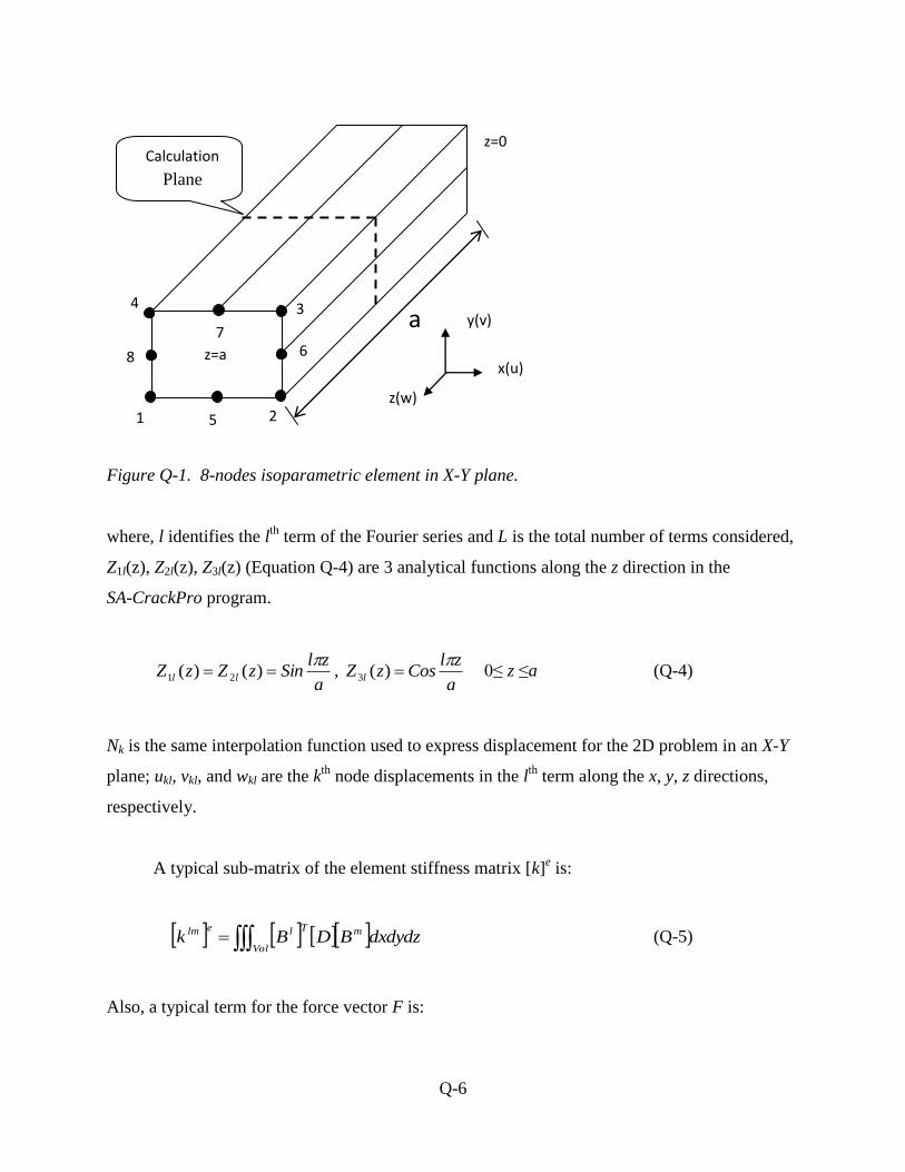
In the SA-CrackPro program, the 8 node isoparametric elements (in the X-Y plane, see

Figure Q-1) are used, and the displacement functions are given by Equation Q-3:

L

l k

lklk zZuNzyxu1

8

1

1 )(),,(

L

l k

lklk zZvNzyxv1

8

1

2 )(),,( (Q-3)

L

l k

lklk zZwNzyxw1

8

1

3 )(),,(

Q-6

Figure Q-1. 8-nodes isoparametric element in X-Y plane.

where, l identifies the lth

term of the Fourier series and L is the total number of terms considered,

Z1l(z), Z2l(z), Z3l(z) (Equation Q-4) are 3 analytical functions along the z direction in the

SA-CrackPro program.

a

zlSinzZzZ ll

)()( 21 ,

a

zlCoszZ l

)(3 0≤ z ≤a (Q-4)

Nk is the same interpolation function used to express displacement for the 2D problem in an X-Y

plane; ukl, vkl, and wkl are the kth

node displacements in the lth

term along the x, y, z directions,

respectively.

A typical sub-matrix of the element stiffness matrix [k]e is:

Vol

mTlelm dxdydzBDBk (Q-5)

Also, a typical term for the force vector F is:

a

1 2

6

3

7

4

8

5

x(u)

z(w)

y(v)

Calculation

Plane

z=a

z=0

Q-7

Vol

lTlel dxdydzpNF (Q-6)

Where, l and m identify the lth

and mth

terms of the Fourier series, respectively, and [B] is the

strain-displacement matrix.

As pointed out by Zienkiewicz (55), the matrix given in Equation Q-5 contains the

following integrals:

a

dza

zm

a

zlI

01 cossin

a

dza

zm

a

zlI

02 sinsin

(Q-7)

a

dza

zm

a

zlI

03 coscos

The integrals exhibit the orthogonal property which ensures that:

I2 = I3 = 0 for l ≠ m (Q-8)

Also, this orthogonal property causes the matrix [k]e to become diagonal. The final assembled

equations for the problem have the following form:

0.........

2

1

2

1

22

11

LLLL F

F

F

K

K

K

(Q-9)

Equation Q-9 shows that the large system of equations splits into L separate problems. As

noted by Zienkiewicz (54), this orthogonal property is of extreme importance for the SA FE

method, because, if the expansion of the loading factors involves only one term for a particular

harmonic, then only one set of simultaneous equations needs to be solved. Thus, what was

originally a 3D problem now has been reduced to a 2D model problem. More theoretical

Q-8

justification can be found in the literature (56). Here it should be noted that, for each problem

calculation, the SA FE method provides the output only along a single X-Y plane at a user

specified z-coordinate. An example of such a plane is shown by broken lines in Figure Q-1.

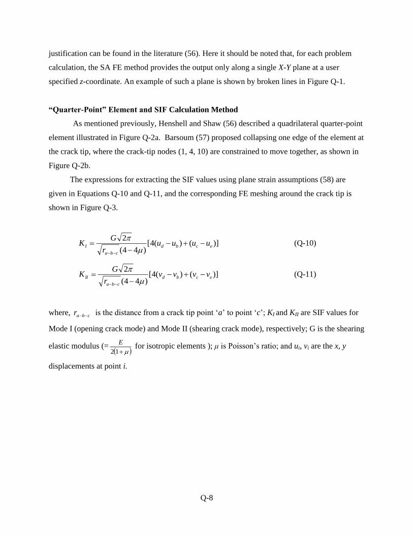
“Quarter-Point” Element and SIF Calculation Method

As mentioned previously, Henshell and Shaw (56) described a quadrilateral quarter-point

element illustrated in Figure Q-2a. Barsoum (57) proposed collapsing one edge of the element at

the crack tip, where the crack-tip nodes (1, 4, 10) are constrained to move together, as shown in

Figure Q-2b.

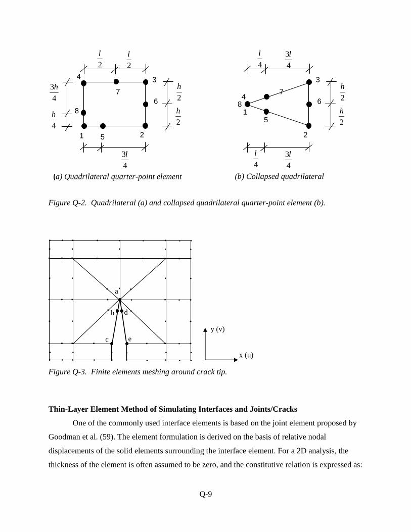
The expressions for extracting the SIF values using plane strain assumptions (58) are

given in Equations Q-10 and Q-11, and the corresponding FE meshing around the crack tip is

shown in Figure Q-3.

)]()(4[)44(

2ecbd

cba

I uuuur

GK

(Q-10)

)]()(4[)44(

2ecbd

cba

II vvvvr

GK

(Q-11)

where, cbar is the distance from a crack tip point „a‟ to point „c‟; KI and KII are SIF values for

Mode I (opening crack mode) and Mode II (shearing crack mode), respectively; G is the shearing

elastic modulus (= 12

E for isotropic elements ); μ is Poisson‟s ratio; and ui, vi are the x, y

displacements at point i.

Q-9

Figure Q-2. Quadrilateral (a) and collapsed quadrilateral quarter-point element (b).

Figure Q-3. Finite elements meshing around crack tip.

Thin-Layer Element Method of Simulating Interfaces and Joints/Cracks

One of the commonly used interface elements is based on the joint element proposed by

Goodman et al. (59). The element formulation is derived on the basis of relative nodal

displacements of the solid elements surrounding the interface element. For a 2D analysis, the

thickness of the element is often assumed to be zero, and the constitutive relation is expressed as:

a

b

c e

d

y (v)

x (u)

1 2

6

3

7

4

8

5

4

l

4

3l

2

l

2

l

2

h

2

h

4

3h

4

h

4

3l

1

2

6

3

7 4

8

5

4

l

4

l

4

3l

2

h

2

h

(a) Quadrilateral quarter-point element (b) Collapsed quadrilateral

quarter-point element.

Q-10

r

r

i

r

r

s

nn

u

vC

u

v

k

k][

0

0

(Q-12)

where, σn is the normal stress; τ is the shear stress; kn is the normal stiffness; ks is the shear

stiffness; vr and ur are the relative normal and shear displacements, respectively; and [C]i is the

constitutive matrix for the interface or joint element.

Based on the assumption that the structural and geological media do not overlap at

interfaces, a high value, on the order of 108-10

12 units, is assigned for the normal stiffness, kn.

However, it is arbitrary for adopting such high values. Furthermore, for modes such as

debonding, the solutions are often unreliable (60).

As an improvement, Desai (60) proposed a method that uses a thin solid element to

simulate interface behavior. Since the proposed element essentially represents a solid element of

small finite thickness and a thin layer of material between two bodies, it is often referred to as a

“thin-layer” element. The distinguishing features of Desai‟s work lie in the special treatment of

the constitutive laws for the thin-layer element which considers the coupling effects of normal

stiffness and shearing stiffness. Often, it was found that satisfactory results can be obtained by

assigning the interface normal component the same properties as the adjacent geological

material.

In the SA-CrackPro program, the interface and/or joint elements are defined as the

orthotropic elements which have the same elastic modulus as that of the adjacent layers, but vary

the shearing modulus to consider the shearing loading transfer between layers. This is one of the

simplified applications of Desai‟s thin-layer method.

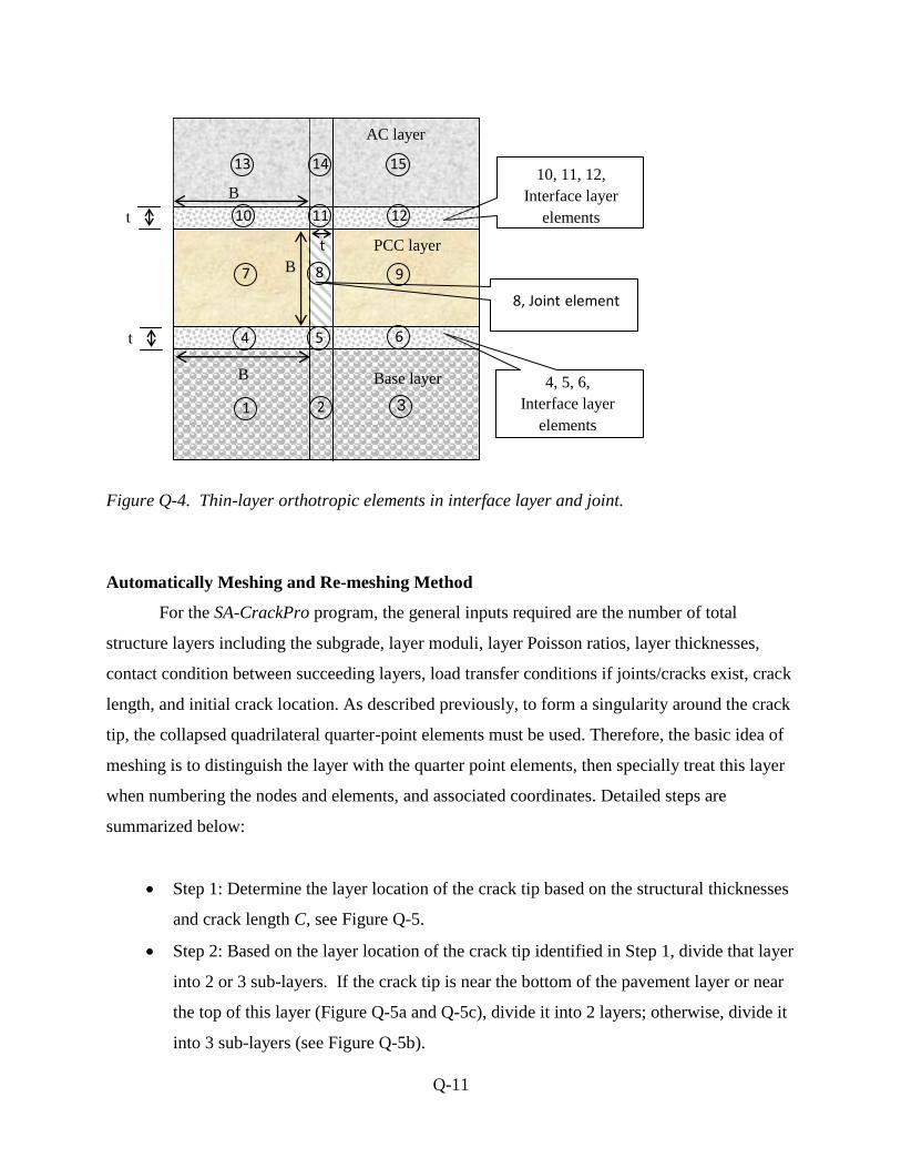
Regarding the thickness of the “thin-layer”, Desai concluded that satisfactory simulation

of the interface behavior can be obtained for t/B ratios (see Figure Q-4) in the range from 0.01 to

0.1(54). Pande and Sharma (61) reported that thin elements also provided satisfactory results for

much lower t/B ratios. In the SA-CrackPro program, the t/B ratios were in the range from 0.0002

to 0.1. After massive SIF calculations, these ratios were found to be able to provide stable and

reasonable SIF results.

Q-11

Figure Q-4. Thin-layer orthotropic elements in interface layer and joint.

Automatically Meshing and Re-meshing Method

For the SA-CrackPro program, the general inputs required are the number of total

structure layers including the subgrade, layer moduli, layer Poisson ratios, layer thicknesses,

contact condition between succeeding layers, load transfer conditions if joints/cracks exist, crack

length, and initial crack location. As described previously, to form a singularity around the crack

tip, the collapsed quadrilateral quarter-point elements must be used. Therefore, the basic idea of

meshing is to distinguish the layer with the quarter point elements, then specially treat this layer

when numbering the nodes and elements, and associated coordinates. Detailed steps are

summarized below:

Step 1: Determine the layer location of the crack tip based on the structural thicknesses

and crack length C, see Figure Q-5.

Step 2: Based on the layer location of the crack tip identified in Step 1, divide that layer

into 2 or 3 sub-layers. If the crack tip is near the bottom of the pavement layer or near

the top of this layer (Figure Q-5a and Q-5c), divide it into 2 layers; otherwise, divide it

into 3 sub-layers (see Figure Q-5b).

t

1 2 3

4 5 6

7 8 9

10 11 12

13 15 14

t

B

B

t

AC layer

10, 11, 12,

Interface layer

elements

PCC layer

Base layer

8, Joint element

4, 5, 6,

Interface layer

elements

B

Q-12

Step 3: Based on the results from Step 2, renumber the layers and recalculate the

thickness of each sub-layer. Note that all the elements in these sub-layers have the

same material property such as elastic modulus and Poisson ratio. Record the layer

number in which the collapsed quadrilateral quarter-point elements are located.

Step 4: Based on the results from Step 3, number each node and element and determine

the corresponding coordinate of each node, and finally generate the meshing data file.

Step 5: Load the meshing data file, and calculate the related node displacements and

then compute the SIF value based on Equation Q-10 or Q-11.

Step 6: Calculate the crack increment based on Equation Q-1, and re-calculate the total

crack length. If the total crack length is longer than the specified layer thickness, then

stop. Otherwise, go back to Step 1.

Figure Q-5. Finite element meshing and re-meshing based on crack tip location.

SA-CRACKPRO PROGRAM VERIFICATION

The efficiency of the SA method has been confirmed both theoretically and practically by

many researchers (55, 62, 63). As Cheung et al. (63) pointed out that in some cases

computational savings of a factor of 10 or more are possible due to the reduction in dimensional

C

AC Layer AC Layer AC Layer

PCC Layer

(b) Crack tip in the

middle of layer.

(c) Crack tip near the

top of layer.

PCC Layer PCC Layer

C

C

(a) Crack tip near the

bottom of layer.

Q-13

analysis. So in this paper, the major concern is the accuracy of the results of the SA-CrackPro

program.

To verify the accuracy of SA-CrackPro, the side by side comparisons were conducted

between ANSYS-3D (64) and SA-CrackPro under the same loading conditions for a same

hypothetical pavement structure. Two cases were studied: one was a bending load mode for KI

verification and the other was a shearing load mode for KII verification. The detailed information

is presented below.

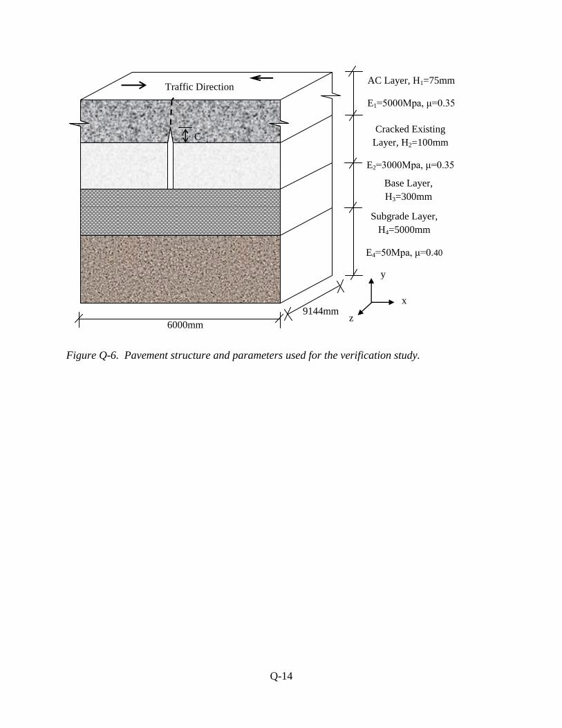
Typical Pavement Structure

Figure Q-6 shows the hypothetical pavement structure used for the verification. It is a

two-laned pavement with shoulders; consisting of 4 layers: Asphalt Concrete Overlay

(AC layer), Cracked Existing layer with a 4 mm wide crack, Base layer, and Subgrade.

The material properties and structural thicknesses are presented in Figure Q-6 as well.

Five different crack lengths were considered in the comparison: C = 7.5, 22.5, 37.5, 52.5, and

67.5 mm, respectively. All pavement layers are assumed to be fully bonded and the zero load

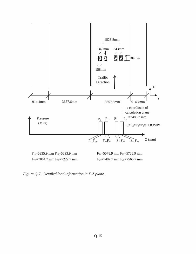
transfer assumption was used. The assumed traffic load is a standard single axle load of 80 kN

with a tire pressure of 0.689 MPa. The detailed traffic loading position and tire contact area are

shown in Figure Q-7.

Two fracture modes were analyzed in this appendix: bending mode and shearing mode.

For the bending mode shown in Figure Q-8a, the axle load is immediately above the crack, and

only KI exists. For the shearing mode shown in Figure Q-8b, the axle load is on one side of the

crack, and both bending and shearing SIFs exist. However, the shearing mode is dominant.

Therefore, only the shearing mode KII were calculated and compared in this case. Here it should

be noted that in all these cases, the calculation plane is the X-Y plane which cuts through the

center of the fourth tire (the outer tire), see Figure Q-8, the z coordinate of this plane is

7486.7mm, see Figure Q-7.

Q-14

Figure Q-6. Pavement structure and parameters used for the verification study.

Traffic Direction AC Layer, H1=75mm

E1=5000Mpa, μ=0.35

Cracked Existing

Layer, H2=100mm

E2=3000Mpa, μ=0.35

Base Layer,

H3=300mm

E3=300Mpa, μ=0.35 Subgrade Layer,

H4=5000mm

E4=50Mpa, μ=0.40

6000mm

x

z

y

9144mm

C

Q-15

Figure Q-7. Detailed load information in X-Z plane.

3657.6mm 3657.6mm 914.4mm 914.4mm

158mm

343mm

1828.8mm

Traffic

Direction

343mm

184mm

m

P1=P2=P3=P4=0.689MPa

F11=5235.9 mm F12=5393.9 mm F21=5578.9 mm F22=5736.9 mm

F31=7064.7 mm F32=7222.7 mm F41=7407.7 mm F42=7565.7 mm

Z (mm)

P1 P2 P3 P4 Pressure

(MPa)

F11F12 F31F32 F41F42 F21F22

z coordinate of

calculation plane

=7486.7 mm

z

x

Q-16

Figure Q-8. Typical load form of bending (a) and shearing (b).

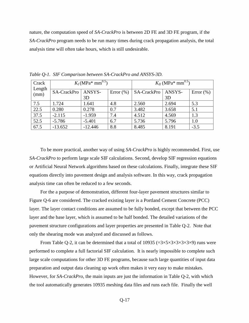
Table Q-1 presents the results from both ANSYS-3D and SA-CrackPro programs. Using

the ANSYS-3D as the reference benchmark, the maximum error is 8.8%. Most errors are around

±5%. It is apparent that SA-CrackPro has an accuracy that is comparable with ANSYS-3D.

SA-CRACKPRO APPLICATIONS

Since the SA method has a much shorter computing time than the 3D FE method, it

becomes possible to directly integrate SA-CrackPro into the pavement design software to predict

the crack propagation. Using SA-CrackPro this way has the benefit that the choice of structure

can be very flexible during design and analysis. However, it is worth noting that, due to the FE

Traffic

Direction

Traffic

Direction

x

z

y

Traffic

Direction

Traffic

Direction

(a) Bending mode: crack front is in the middle of the axle load area.

(b) Shearing load: crack front is at the edge of the axle load area.

Calculation

Plane

Calculation

Plane

Q-17

nature, the computation speed of SA-CrackPro is between 2D FE and 3D FE program, if the

SA-CrackPro program needs to be run many times during crack propagation analysis, the total

analysis time will often take hours, which is still undesirable.

Table Q-1. SIF Comparison between SA-CrackPro and ANSYS-3D.

Crack

Length

(mm)

KI (MPa* mm

0.5)

KII (MPa* mm0.5

)

SA-CrackPro ANSYS-

3D

Error (%) SA-CrackPro ANSYS-

3D

Error (%)

7.5 1.724 1.641 4.8 2.560 2.694 5.3

22.5 0.280 0.278 0.7 3.482 3.658 5.1

37.5 -2.115 -1.959 7.4 4.512 4.569 1.3

52.5 -5.786 -5.401 6.7 5.736 5.796 1.0

67.5 -13.652 -12.446 8.8 8.485 8.191 -3.5

To be more practical, another way of using SA-CrackPro is highly recommended. First, use

SA-CrackPro to perform large scale SIF calculations. Second, develop SIF regression equations

or Artificial Neural Network algorithms based on these calculations. Finally, integrate these SIF

equations directly into pavement design and analysis software. In this way, crack propagation

analysis time can often be reduced to a few seconds.

For the a purpose of demonstration, different four-layer pavement structures similar to

Figure Q-6 are considered. The cracked existing layer is a Portland Cement Concrete (PCC)

layer. The layer contact conditions are assumed to be fully bonded, except that between the PCC

layer and the base layer, which is assumed to be half bonded. The detailed variations of the

pavement structure configurations and layer properties are presented in Table Q-2. Note that

only the shearing mode was analyzed and discussed as follows.

From Table Q-2, it can be determined that a total of 10935 (=3×5×3×3×3×3×9) runs were

performed to complete a full factorial SIF calculation. It is nearly impossible to complete such

large scale computations for other 3D FE programs, because such large quantities of input data

preparation and output data cleaning up work often makes it very easy to make mistakes.

However, for SA-CrackPro, the main inputs are just the information in Table Q-2, with which

the tool automatically generates 10935 meshing data files and runs each file. Finally the well

Q-18

organized result summary file is generated automatically, which is ready to perform regression

analysis. Note that in this case, the total input work only requires several minutes, and as long as

these inputs are right, the 10935 definitely correct results will be obtained. A comparison

between the calculated SIF-values and those predicted by a regression model is shown in

Figure Q-9.

Table Q-2. Structure and material properties used for SIF analysis.

Main Parameter Range Selected Values Count Number

H1 (AC Layer

Thickness, mm) 38-75 38, 75, 150 3

E1 (AC Layer

Modulus, MPa) 1000-20000 1000, 3000, 6000, 10000, 20000 5

H2 (Existing Layer

Thickness, mm) 200-400 200, 300, 400 3

E2 (Existing Layer

Moudlus, MPa) 20000-40000 20000, 30000, 40000 3

H3 (Base Layer

Thickness, mm) 100-400 100, 200, 400 3

E3 (Base Layer

Modulus, MPa) 100-10000 100, 1000, 10000 3

H4 (Subgrade

Thickness, mm) 5000 5000 1

E4 (Subgrade

Modulus, MPa) 30-150 50

* 1

c/H1 (ratio of crack

length over H1) 0.1-0.9 0.1, 0.2, 0.3, 0.4, 0.5, 0.6, 0.7, 0.8, 0.9 9

* Since subgrade modulus did not have much influence on KII value, only one typical value was used.

SUMMARY AND CONCLUSIONS

A new pavement crack propagation analysis tool named SA-CrackPro was developed in

this appendix. The main features of SA-CrackPro are 1) computational efficiency, 2)

isoparametric quadratic "quarter-point" elements for SIF calculation, 3) thin-layer elements to

simulate pavement layer contact condition and/or load transfer efficiency at joints/cracks,

and 4) automatically meshing and re-meshing technique for crack propagation analysis.

Additionally, a detailed discussion of these technical key components of SA-CrackPro was

provided. Specifically, SA-CrackPro provides comparably accurate SIF computations which

Q-19

were verified by ANSYS-3D. Since SA-CrackPro has much shorter computing time than the

3D FE method, it becomes possible to be directly integrated into pavement design and analysis

software. Also, this tool can be used to perform large scale SIF calculations very easily. Based

on these calculation results, the SIF regression equations can be developed, as demonstrated in

this paper. In summary, this new tool: SA-CrackPro can provide efficient and satisfactory

solutions to pavement crack propagation analysis.

Figure Q-9. SIF predicted by regression equation vs. SIF calculated by SA-CrackPro.