APPENDIX D: SAMPLE OF UNCERTAINTY ANALYSIS

Pioro, I.L. and Duffey, R.B., 2007. Heat Transfer and Hydraulic Resistance at Supercritical

Pressures in Power Engineering Applications, ASME Press, New York, NY, USA, 334

pages.

The proposed uncertainty analysis1 is based on our current experience with heat-transfer

and pressure-drop experiments in supercritical water (Kirillov et al. 2005; Pis’menny et al. 2005)

and carbon dioxide (Pioro and Khartabil 2005) and on our long-term experience in conducting

heat-transfer experiments at subcritical pressures (Guo et al. 2006; Bezrodny et al. 2005; Leung

et al. 2003; Pioro et al. 2002a,b, 2001, 2000; Pioro 1999, 1992; Pioro and Pioro 1997; Kichigin

and Pioro 1992; Pioro and Kalashnikov 1988; Pioro 1982). Also, basic principles of the theory

of thermophysical experiments and their uncertainties were applied (Coleman and Steel 1999;

Hardy et al. 1999; Guide… 1995; Holman 1994; Moffat 1988; Gortyshov et al. 1985; Topping

1971).

In general, an uncertainty analysis is quite complicated process in which some

uncertainties2 (for example, uncertainties of thermophysical properties (for details, see NIST

(2002)), uncertainties of constants, etc.) may not be known or may not be exactly calculated.

Therefore, applying the engineering judgement is the only choice in some uncertainty

calculations.

This section summarizes instrument calibrations and uncertainty calculations for the

measured parameters such as temperature, pressure, pressure drop, mass-flow rate, power, tube

dimensions, etc. and for the calculated parameters such as mass flux, heat flux, etc. in

supercritical heat-transfer and pressure-drop tests. Uncertainties for these parameters are based

on the RMS of component uncertainties. All uncertainty values are at the 2σ level, unless

otherwise specified.

1 The authors of the current monograph express their appreciation to D. Bullock and Y. Lachance (CRL AECL)

for their help in preparation of this uncertainty analysis. 2 Uncertainty refers to the accuracy of measurement standards and equals the sum of the errors that are at work to

make the measured value different from the true value. The accuracy of an instrument is the closeness with

which its reading approaches the true value of the variable being measured. Accuracy is commonly expressed

as a percentage of a measurement span, measurement value or full-span value. Span is the difference between

the full-scale and the zero scale value (Mark’s Standard Handbook for Mechanical Engineers 1996).

Calibration of the instruments used in the tests was performed either in situ, e.g., power

measurements, test-section thermocouples, etc., or at an instrumentation shop, e.g., pressure

transducers and bulk-fluid temperature thermocouples. In general, instruments were tested

against a corresponding calibration standard.

When the same calibration standard is used for serial instruments, the calibration standard

uncertainty is treated as a systematic uncertainty. In general, high accuracy calibrators were

used, hence systematic errors for calibrated instruments are considered to be negligible. All

other uncertainties are assumed to be random. Also, errors correspond to the normal distribution.

Usually, the uncertainties have to be evaluated for three values of the corresponding parameter:

minimum, mean and maximum value within the investigated range.

Uncertainties are presented below for instruments, which are commonly used in heat-

transfer and pressure-drop experiments. It is important to know the exact schematics for sensor

signal processing. Some commonly used cases, which are mainly based on a DAS recording, are

shown in Figure D1 for thermocouples and in Figure D2 for RTDs, pressure cells and differential

pressure cells.

mV

Sensor - Thermocouple

1

2

Sensor

Referencejunction

Gate

card

3 4

DAS

5

A/D

convert

or

Alg

orith

m

Dis

pla

y/S

tora

ge

Figure D1. Schematic of signal processing for temperature (based on thermocouple)

measurements. Numbers in figure identify uncertainty of particular device in measuring

circuit: 1 – sensor uncertainty, 2 – reference junction uncertainty, 3 – Analog Input (A/I)

uncertainty, 4 – Analog-to-Digital (A/D) conversion uncertainty, and 5 – DAS algorithm

uncertainty.

4-20 mA

Resis

tor

250

Sensor

Gate

card

1-5

V

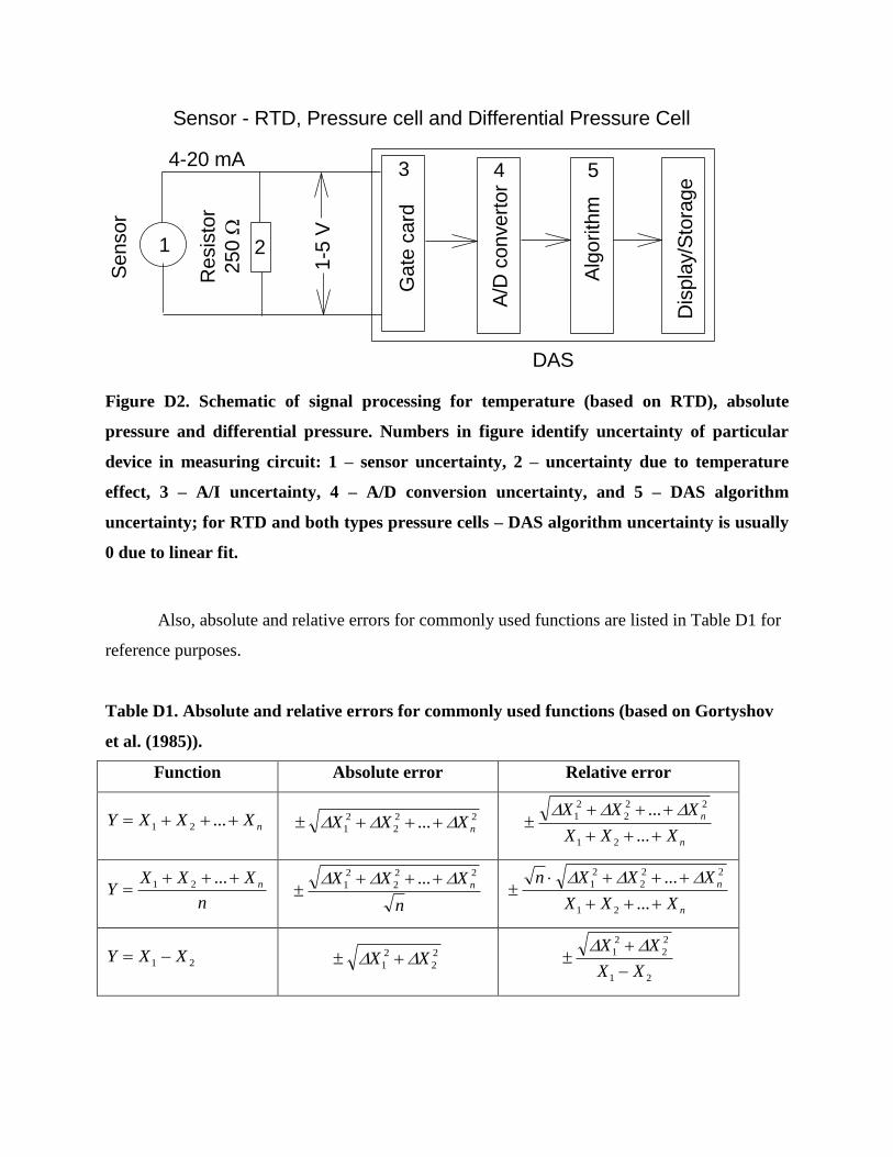
Sensor - RTD, Pressure cell and Differential Pressure Cell

1 2

3 4

DAS

5

A/D

convert

or

Alg

orith

m

Dis

pla

y/S

tora

ge

Figure D2. Schematic of signal processing for temperature (based on RTD), absolute

pressure and differential pressure. Numbers in figure identify uncertainty of particular

device in measuring circuit: 1 – sensor uncertainty, 2 – uncertainty due to temperature

effect, 3 – A/I uncertainty, 4 – A/D conversion uncertainty, and 5 – DAS algorithm

uncertainty; for RTD and both types pressure cells – DAS algorithm uncertainty is usually

0 due to linear fit.

Also, absolute and relative errors for commonly used functions are listed in Table D1 for

reference purposes.

Table D1. Absolute and relative errors for commonly used functions (based on Gortyshov

et al. (1985)).

Function Absolute error Relative error

nXXXY ...21 22

2

2

1 ... nXXX n

n

XXX

XXX

...

...

21

22

2

2

1

n

XXXY n

...21 n

XXX n

22

2

2

1 ...

n

n

XXX

XXXn

...

...

21

22

2

2

1

21 XXY 2

2

2

1 XX 21

2

2

2

1

XX

XX

21 XXY 212

2

21 XXXX

2

2

2

2

1

1

X

X

X

X

XaY Xa X

X

nXY XXn n 1 X

Xn

XY sin XX cos XX ctg

XY cos XX sin XX tg

XY tg X

X2cos

X

X

2sin

2

XY ctg X

X2sin

X

X

2sin

2

D.1 Temperature

For the calibrated thermocouples, the following linear characteristics were found:

b +V a = V measact , (D1)

where Vact is the “actual” value3 of the given parameter, Vmeas is the value measured by the given

instrument, and a and b are the calibration coefficients.

D.1.1 Measured Bulk-Fluid Temperature

The test section (see Figures 10.5 and 10.6) has three thermocouples to measure the inlet

and outlet bulk-fluid temperatures. Also, the temperature at the flowmeter is monitored by

thermocouple for fluid density calculations.

The test-section inlet and outlet bulk-fluid temperatures were measured with sheathed K-

type thermocouples (for thermocouple signal processing, see Figure D1). These thermocouples

3 The value obtained from the calibration standard.

were calibrated against the temperature standard RTD over the temperature range from 0 to

100ºC. For the reference RTD, the maximum error was ±0.3ºC. The maximum uncertainty of a

data fit for inlet and outlet bulk-fluid temperature measurements is listed in Table D2.

Table D2. Linear coefficients for inlet and outlet temperature thermocouples (from

instrument calibration records).

TC Coefficient Uncertainty, ºC Number of points

– a b Maximum (2σ) –

TE-1 1.000 –0.1798 0.12 5

TE-2 0.9980 0.1502 0.12 5

TE-3 0.9985 0.0980 0.12 5

The inlet and outlet bulk-fluid measurement uncertainties4 are as follows:

Calibration system

uncertainty

0.3ºC

Thermocouple sensor

accuracy after linear fit

0.12ºC

A/I accuracy

0.06°C, i.e., 0.025% of f.s.;

C

mV0.045

mV100.00025;

where f.s. is the full scale

A/D resolution accuracy

(minimum 1 bit) 0.03°C

C

mV0.045counts8192

(f.s.)mV10, where 0.045

mV/ºC is the conversion rate, i.e., 4.509 mV for 100ºC

(The Temperature Handbook 2000)

Reference junction 0.4ºC

4 All inputs are from instrument calibration records and device manuals unless otherwise specified.

accuracy

For a given test-section inlet or outlet temperature t, the uncertainty t is given by

t

.+

t

.+

t

. =

t

t222

03012030. (D2)

The first term is the maximum error of the calibration system (±0.3ºC). The second term is the

maximum error for the sheathed thermocouple (≤100ºC), obtained from the calibration. The

third term is the uncertainty introduced by the DAS, i.e., the A/D resolution uncertainty

(±0.03ºC). Note that since the calibration was done in situ using the DAS as the measuring

system for the RTD and for the calibrated thermocouples, the uncertainty introduced by the

reference junction and the A/I accuracy was included in calibration curves.

All bulk-fluid temperature thermocouples were calibrated in situ, only within the range of

0 – 100ºC. Therefore, individual correction factors were implemented for each thermocouple

within the range of 0 – 100ºC (see Table D2). For this range of temperatures, the uncertainty t

is

for tmin = 20ºC t = ±0.32ºC (or ±1.62%), and

for t = 100ºC t = ±0.32ºC (or ±0.32%).

Beyond this range, thermocouple uncertainties were taken as per The Temperature Handbook

(2000), i.e., 2.2°C.

Thermocouple installed near the flowmeter was calibrated using another calibrating

system and procedure. All inputs below are from instrument calibration record and device

manuals unless otherwise specified.

Calibration system uncertainty:

0.5°C, i.e., 222 041050060 ... , where the first term is the accuracy of standard RTD,

the second term is the accuracy of thermocouple signal measuring device and the third term is

the accuracy of RTD signal measuring device (all uncertainties are in ºC).

TC maximum calibration 0.53°C

accuracy5 (>2σ) within 0.0 –

45.0ºC

A/I accuracy 0.06°C, i.e., 0.025% of f.s.

C

mV0.045

mV100.00025

A/D resolution accuracy

(minimum 1 bit) 0.03°C

C

mV0.045counts8192

(f.s.)mV10, where

0.045 mV/ºC is the conversion rate, i.e., 4.509

mV for 100ºC (The Temperature Handbook 2000)

Reference junction accuracy 0.02°C

For a given flowmeter bulk-fluid temperature tfm, the uncertainty tfm is given by

TC

outoutoutfmfmTCfm

fm

tttttt

t

2

2222

02.003.006.053.05.0. (D3)

Therefore, the flowmeter bulk-fluid temperature uncertainty is:

for tfm min = 19ºC tfm = ±0.74ºC (or ±3.9%), and

for tfm max = 35ºC tfm = ±0.74ºC (or ±2.1%).

Additional uncertainties due to thermocouple installation and possible electrical pickup

have been minimized by using good engineering practices.

If a bulk-fluid temperature is measured with an RTD, then the following will apply.

The bulk-fluid temperature measurement uncertainties at the 2σ level are characterized

with the following for an RTD (for RTD signal processing, see Figure D2):

5 The TC calibration accuracy is the maximum difference in °C between what the calibration standard measured and

what TC indicated.

Calibration system uncertainty in ºC (from the instrument calibration record):

C0.06C0.05mA16

C100f.s.of0.015%

C100

mA16Readingof%01.0Unc.Sys.Cal.

2

2

,

where the first term is the accuracy of calibrator in which reading is in ºC and f.s. is 30 mA and a

conversion rate is 16 mA for 100ºC; and the second term is the accuracy of standard RTD.

The RTD accuracy after linear fit, i.e., maximum deviation (from the instrument calibration

record), is about 0.08°C;

A/I accuracy (from the device manual):

0.032°C (0.025% of f.s.), i.e.,

C

V0.04

(f.s.) V 5.120.00025.

A/D conversion accuracy (minimum 1 bit accuracy) (from the device manual):

0.016°C, i.e.,

C

V0.04counts8192

(f.s.)V5.12, where 0.04 V/ºC is the conversion rate, i.e., 4 V for

100ºC (from the instrument calibration record).

DAS algorithm uncertainty is 0 due to a linear fit.

Therefore, for a given test-section inlet temperature, its uncertainty (Δt) is given by

2222016.0032.008.0Unc.Sys.Cal.

ttttt

t. (D4)

The resulting uncertainties in the bulk-fluid temperature are

For t = 10°C Δt = ±0.10°C (or 1.2%); and

For t = 50°C Δt = ±0.11°C (or 0.2%).

If the bulk-fluid temperature is measured with several devices installed in a one cross

section (for example, two RTDs and one thermocouple), the following equation may apply:

t

ttt

t

t TCRTDRTD

3

)()()( 22

2

2

1 . (D5)

In this case, the resulting uncertainty will be close to the larger uncertainty, i.e., the

thermocouple uncertainty. Therefore, if several devices have to be used for measuring a non-

uniform temperature or any other parameter, they have to be with a similar accuracy.

D.1.2 External Wall Temperature

Temperatures for the test-section external surface (see Figure 10.6) were measured using

fast-response K-type thermocouples (see Figure D3). In general, thermocouple uncertainties for

K-type thermocouples are 2.2°C within a range of 0 – 277ºC (The Temperature Handbook,

2000). However, all fast-response thermocouples were calibrated in situ within a range of 0 –

100ºC prior to use (for details, see below). Therefore, individual correction factors were

implemented for each thermocouple within the range of 0 – 100ºC. Beyond this range,

thermocouple uncertainties were taken as per The Temperature Handbook (2000), i.e., 2.2°C.

Flattened bead

D=1 mm, =0.16 mm

OD=0.3 mm30 AWG

Tefloncoating

25

mm

19 mm

0.67 mm

=0.14 mm

To

p

- h

igh

te

mp

era

ture

po

lym

er

( =

0.1

5 m

m)

Bo

tto

m -

hig

h t

em

pe

ratu

re f

ibe

r-re

info

rce

d p

oly

me

r

with

se

lf-a

dh

esiv

e b

ackin

g (

=0

.15

mm

)

Fast response K-type thermocouple (0.3 s response time)

Foil

8.2

mm

1 mm

Figure D3. Sketch drawing of fast-response K-type thermocouple.

All K-type thermocouples were calibrated against the temperature calibration standard

(i.e., the reference RTD) over the temperature range from 0 to 100ºC. These thermocouple

assemblies were immersed in a liquid bath thermostat together with the RTD. For the reference

RTD, the maximum uncertainty is ±0.3ºC. The combined uncertainty6 for wall temperature

measurements is as follows:

Calibration system

accuracy

0.3ºC

Thermocouple sensor

accuracy after linear fit

0.16ºC max at values ≤100°C

A/I accuracy

0.06°C, i.e., 0.025% of f.s.

C

mV0.045

mV100.00025

A/D resolution accuracy

(minimum 1 bit) 0.03°C

C

mV0.045counts8192

(f.s.)mV10, where 0.045

mV/ºC is the conversion rate, i.e., 4.509 mV for 100ºC

(The Temperature Handbook 2000)

For a given test-section wall temperature t, the uncertainty t is given by

t

.+

t

.+

t

. =

t

t222

03016030. (D6)

The first term is the maximum error of the calibration system (±0.3ºC). The second term is the

maximum error of the sheathed thermocouple (≤100ºC), obtained from the calibration. The third

term is the uncertainty introduced by the DAS, i.e., the A/D resolution uncertainty (±0.03ºC).

Note that since the calibration was done in situ using the DAS as the measuring system for the

RTD and the calibrated thermocouples, the uncertainty introduced by the reference junction and

the A/I accuracy was included in calibration curves.

Within the calibrated range of measured temperatures, i.e., from 0 to 100ºC, the

6 All inputs are from instrument calibration records and device manuals unless otherwise specified.

uncertainty t is

for tmin = 25ºC t = ±0.34ºC (or ±1.36%), and

for t = 100ºC t = ±0.34ºC (or ±0.34%).

Also, the external wall temperatures measured with fast-response thermocouples were

compared to the inlet and outlet bulk-fluid temperatures measured with sheathed thermocouples,

at 0 power and 0 mass flux through the test section (see Figure D4). The comparison showed

that, in general, all measured temperatures were within ±0.3ºC.

Axial Location, mm

0 500 1000 1500 2000 2500

Te

mp

era

ture

, oC

23

24

25

26

Tin

Tout T

out mixer

External wall temperature

Carbon dioxide, pout

=7.07 MPa, p=0 kPa,

G=0 kg/m2s, Q=0.0 kW, q=0.0 kW/m

2

Tin, T

out, T

out mixer, T

w ext are measured values

+0.3oC

-0.3oC

ave

extwT

Figure D4. Temperature profile along test section at 0 power and 0 mass flux values.

D.2 Absolute Pressure

A high-accuracy gauge pressure cell with a range of 0 – 10,000 kPa (0 – 10 MPa) was

used for the outlet-pressure measurements (for pressure signal processing, see Figure D2). A

small correction (77.2 kPa) is applied in the DAS program for the elevation difference between

the pressure tap and transmitter. The combined uncertainty for absolute pressure measurements

is as follows.

Accuracy of gauge pressure cell (from the calibration record) is 0.1% of calibrated span (10,000

kPa), and this accuracy was verified during the calibration check.

Calibration system uncertainty in kPa (from the instrument calibration record):

22

Readingof0.1%mA16

kPa10000f.s.of0.015%

kPa10000

mA16Readingof0.015%Unc.Sys.Cal.

, where the

first term is the accuracy of calibrator in which reading is in kPa and f.s. is 30 mA and

conversion rate is 16 mA for 10000 kPa; and the second term is the accuracy of tester.

Uncertainty due to temperature effect in 250-Ω resistor:

±0.1%.

A/I accuracy (from the device manual):

3.2 kPa, i.e., 0.025% of f.s., i.e., 5.12 V

kPa

V0.0004

V5.120.00025.

A/D conversion accuracy (minimum 1 bit accuracy) (from the device manual):

1.56 kPa

kPa

V0.0004counts8192

(f.s.)V5.12, where 0.0004 V/kPa is the conversion rate, i.e., 4 V

for 10,000 kPa (from the instrument calibration record).

For a given test-section outlet pressure p, the uncertainty p is given by

2222

A/DA/I

100

1.0100000010

ppp

.

p

p, (D7)

For the range of p from 7.6 to 8.8 MPa, the uncertainty p is given by

for pmin = 7600 kPa p = ±13.1 kPa (or ±0.17%),

for p = 8400 kPa p = ±13.5 kPa (or ±0.16%).

for pmax = 8800 kPa p = ±13.8 kPa (or ±0.16%).

D.3 Differential-Pressure Cells

Five differential-pressure transducers for measuring test-section pressure drops (for

differential-pressure signal processing, see Figure D2) were connected to the corresponding

pressure taps installed as shown in Figure 10.6. They were used for measuring the test-section

axial pressure gradient and the overall pressure drop. Also, one differential-pressure transducer

was used to measure a pressure drop across the flowmeter (see Figure 10.5). All these pressure

drops were measured using pressure transmitters.

A calibrator and a pressure module were used for the calibration check of the differential-

pressure transducers. Basic characteristics of the test-section and flowmeter differential-pressure

cells are listed in Table D3.

Table D3. Basic characteristics of differential-pressure cells.

Instrument

Name

Description Output Output

kPa

Span

kPa

Accuracy

±% of span

PDT-1 Total test-section pressure

drop

10–50 mV 0–300 300 0.5

PDT-2 Test-section pressure drop 1–5 V 0–50 50 0.5

PDT-3 Test-section pressure drop 1–5 V 0–50 50 0.5

PDT-4 Test-section pressure drop 1–5 V 0–50 50 0.5

PDT-5 Test-section pressure drop 1–5 V 0–50 50 0.5

PDT-FM-1 Orifice-plate pressure drop 10–50 mV 0–37 37 0.5

Accuracy, includes combined effects of linearity, hysteresis and repeatability in % of a

calibrated span are listed in Table D3.

Calibration system uncertainty in kPa (from instrument calibration records):

2

2

f.s.of0.05%mA16

kPaSpanf.s.of0.015%

kPaSpan

mA16Readingof0.015%Unc.Sys.Cal.

, where the

first term is the accuracy of process calibrator in which reading is in kPa, f.s. is 30 mA and

conversion rate is 16 mA for span in kPa; and the second term is the accuracy of calibrator in

which f.s. is 690 kPa (100 psig).

Uncertainty due to temperature effect in 250-Ω resistor:

±0.1%.

A/I accuracy (from a device manual):

0.025% of f.s., i.e.,

kPaSpan

V4

V5.120.00025.

A/D conversion accuracy (minimum 1 bit accuracy) (from a device manual):

kPaSpan

V4counts8192

(f.s.)V5.12.

For a given pressure drop (Δp) for PDT-1, PDT-2 to PDT-5 and PDT-FM-1, the

uncertainty Δ(Δp) is given by

2222

A/DA/I

100

1.0kPain span of %)(

pppp

p

. (D8)

For the range of the total p from 5 to 70 kPa, the uncertainty p) for PDT-1 is given by

for pmin = 5 kPa p) = ±1.50 kPa (or ±30.1%), and

for pmax = 70 kPa p) = ±1.51 kPa (or ± 2.2%).

For the range of the local p from 5 to 30 kPa, the uncertainty p) for PDT-2 – PDT-5 is

given by

for pmin = 5 kPa p) = ±0.25 kPa (or ±5.0%), and

for pmax = 30 kPa p) = ±0.25 kPa (or ±0.84%).

For the local p equals to 37 kPa, the uncertainty p) for PDT-FM-1 is given by

for pmin = 1.5 kPa p) = ±0.19 kPa (or ±12.5%), and

for pmax = 16.9 kPa p) = ±0.19 kPa (or ± 1.1%).

D.4 Mass-Flow Rate

The loop mass-flow rate FM-1 (see Figure 10.5) is measured by a small orifice plate7

with an orifice diameter of 0.308", and monitored by a differential-pressure cell with the range of

0 – 37 kPa. This cell has a square root output, with an accuracy of ±0.5% of full scale. The

square root output is converted in the program to obtain kPa for use in the following flow

equation, for a mass-flow rate of 0 – 0.24 kg/s (see Figure D4):

pCm fl , (D9)

where Cfl = 0.00130 is the constant (White 1994), ρ is the density at the orifice plate in kg/m3,

and Δp is the pressure drop across the orifice plate in kPa. It is known that orifice-plate

flowmeters usually have a working range within (0.3 and 1)·mmax, i.e., 0.08 – 0.24 kg/s (The

Flow and Level Handbook 2001).

In general, the constant Cflow is a function of Reynolds number (see Figure D5).

However, this effect is minor within the investigated range of Reynolds numbers (Re = 57,000 –

1,130,000).

7 This small diameter orifice plate is a non-standard orifice plate, because International Standard ISO 5167-

2:2003(E), “Measurement of fluid flow by means of pressure differential devices inserted in circular-cross section

conduits running full – Part 2: Orifice Plates”, applies only to orifice plates with a diameter not less than 12.5 mm.

Flowmeter Pressure Drop, kPa

0 5 10 15 20 25 30 35 40

Mass F

low

Rate

, kg/s

0.000

0.025

0.050

0.075

0.100

0.125

0.150

0.175

0.200

0.225

0.250

Mass F

lux, kg/m

2s

0

500

1000

1500

2000

2500

3000

3500

4000

4500

Carbon dioxide, p=8.36 MPa,

t=25oC, =786.5 kg/m

3

Pm 00130.0

Re

0.0 200.0x103 400.0x103 600.0x103 800.0x103 1.0x106 1.2x106

Cflo

w*1

05

128

130

132

134

136

138

140

Figure D4. Flow-measurement curve. Figure D5. Effect of Reynolds number

on flow constant

We attempted to calibrate the flowmeter FM-1 with water using the direct weighting

method (Hardy et al. 1999) within the supercritical CO2 investigated Reynolds numbers range.

Due to significantly different values of water dynamic viscosity compared to those of

supercritical carbon dioxide and restrictions applied to the maximum water flow and its

temperature, the flowmeter was calibrated (see Figure D6) within a lower range of Reynolds

numbers (Re = 2,700 – 27, 000) compared to those of supercritical carbon dioxide (Re = 57,000

– 1,130,000).

Orifice Pressure Drop, kPa

0 2 4 6 8 10 12 14 16 18 20

Mass F

low

Rate

, g/s

0

20

40

60

80

100

120

140

160

180

Mass F

lux, kg/m

2s

0

500

1000

1500

2000

2500

3000

3500recorded by DAS using Equation (C7)

measured by direct weighting method

Water, atmospheric pressure,

twater

=18oC, Re=2,700-27,000

Orifice Pressure Drop, kPa

0.01 0.02 0.04 0.1 0.2 0.4 1 2 4 6 10 20

Mass F

low

Rate

, g/s

5

7

10

15

20

30

50

70

100

120

150

180

6

8

40

80

60

Mass F

lux, kg/m

2s

100

200

500

700

1000

1500

2000

2500

30003500

150

300

400

recorded by DAS using Equation (C7)

measured by direct weighting method

Water, atmospheric pressure,

twater

=18oC, Re=2,700-27,000

(a) (b)

Figure D6. Calibration results for FM-1 orifice-plate flowmeter: (a) linear scale, and (b)

logarithmic scale.

However, the calibration results showed that Equation (D9) is reasonably accurate (a

mean error is –0.15% and an RMS error is 0.5%) for flows that are not less than 0.045 kg/s. This

finding is consistent with heat-balance error data obtained in supercritical CO2. However, the

heat-balance error data for m < 0.045 kg/s show the opposite trend, i.e., steeper slope than that

shown in Figure D6b. Mass-flow rates lower than 0.045 kg/s were calculated using:

inout HH

POWm

. (D10)

In general, flow-rate measurement uncertainty within the range of m = 0.045 – 0.24 kg/s

is given by:

222

1

1 5.05.0

p

p

C

C

m

m

. (D11)

The estimated uncertainty in the constant C1 is ±0.08% as a result of the minor effect of

Reynolds number on the constant within the investigated range (White 1994).

Temperature, pressure (see Figure 10.5) and NIST software (2002) were used for the CO2

density calculation. At pressures up to 30 MPa and temperatures up to 249.9ºC (523 K), the

estimated uncertainty in density (NIST 2002) varies up to 0.05%. Also, additional uncertainty in

density arises from variations in density within the measured temperature uncertainty of ±1.1ºC.

This additional uncertainty is about ±1.1% at p = 8.36 MPa and t = 19ºC, and ±5.0% at p = 8.8

MPa and t = 35ºC. Therefore, the total uncertainty in density is

0110100

11

100

05022

...

at p = 8.36 MPa and t = 19ºC (D12)

and

050100

05

100

05022

...

at p = 8.8 MPa and t = 35ºC. (D13)

However, the vast majority of the experimental data were obtained at pressure of 8.36

MPa. Therefore, the uncertainty value of 0.011 was used below.

Pressure-drop measurement uncertainties for PDT-FT-1/1 are according to Section D.3.

Hence,

for mmin = 46 g/s m = ±5.7 g/s (or ±12.5%) at t = 19ºC and p = 8.36 MPa, and

for mmax = 155 g/s m = ±2.4 g/s (or ± 1.6%) at t = 19ºC and p = 8.36 MPa.

D.5 Mass Flux

Mass flux, G, is based on mass-flow rate measurements. The uncertainty, G, includes

an error in the estimation of the cross-sectional flow area, Afl = 5.1 10–5

m2. The test section is a

tube of 8.058 mm ID and 10 mm OD, made of Inconel 600, with tolerances of ±0.02 mm. The

uncertainties are as follows:

For ID D = ±0.02 mm (or ±0.25%),

For OD Dext = ±0.02 mm (or ±0.20%), and

For Aflow Afl = 2

DD = ±0.253 mm

2 (or ±0.50%).

The uncertainty, G, is obtained from the following equation:

A

A+

m

m

GA

A m+

GA

m =

G

G

fl

fl

22

2fl

fl

2

fl

2

. (D14)

For the range of interest, the uncertainties, G, are

for Gmin 902 kg/m2·s (mmin = 46 g/s) G = ±112.8 kg/m

2·s (or ±12.5%), and

for Gmax = 3039 kg/m2·s (mmax = 155 g/s) G = ± 49.8 kg/m

2·s (or ± 1.6%).

D.6 Electrical Resistivity

Electrical resistivity is a calculated value (for details, see Equation (C2)) that is based on

measured values of electrical resistance, heated length and tube diameters.

The accuracy of the micro-ohmmeter used in test-section electrical resistance

measurements is ±0.04% of the reading (its readings are in milliohms). The uncertainties in ID

and OD are D =Dext = ±0.02 mm, and in L it is L = ±0.5 mm.

For a given electrical resistivity, the uncertainty ρ is given by

L

L

D

D

D

D+ =

2

ext

ext

2

el

el

22

100

040.. (D15)

The uncertainty in el (ρel = 104.3·10–8

Ohm·m) is

for L = 2461 mm ρel = ±0.212·10–8

Ohm·m (or ±0.20%).

D.7 Total Test-Section Power

The total test-section power is obtained by measuring the current through a 2000 A/100

mV current shunt and the voltage across the test section. These signals are fed into a power-

measuring unit (PMU), where the test-section voltage is scaled down to a 1-V level. Both the

voltage and current signals are fed into isolation amplifiers and then into instrumentation

amplifiers with outputs of 0 – 10 V. The amplifier outputs are fed to the computer analog inputs

and represent a full-scale voltage of 175 V and a full-scale current of 2000 A. These signals are

multiplied in the computer program to represent a 0 – 350 kW power level.

Calibration of the power measurement unit was performed in situ. Test-section voltage

and current inputs were removed from the PMU. Simulated inputs were used to check the

calibration of the unit. A comparison between the computer readings and the calibrated

simulated inputs was used to create a curve fit for the DAS to correct for the differences. The

voltage input from 0 – 110 V DC was simulated with a DC power supply and verified with a

multimeter. The current shunt input was simulated with a calibrator for inputs from 10 to 100

mV, which represents 200 – 2000-A range:

Accuracy of current shunt ±0.25% of reading

Error due to current shunt resistance change ±0.02%

A/D accuracy 0.025% of f.s., 10.00 V

The uncertainty, POWTS, in power measurements (the power is a product of U and I) is

given by

U

U

I

I

POW

POW

TS

TS 1

2

1

2222

100

09.0

100

1.0

100

02.0

100

25.0 . (D16)

The first term is the accuracy of the current shunt, the second term is the effect of a temperature

change on the current shunt, the third term is the error in the test-section voltage drop from the

PMU output of U = +0.1% (0.10 V) up to 100 V, the fourth term is the error in the test-section

current from the PMU output with a maximum offset of I = +0.09% (0.75 A) at 800 A, and the

fifth and sixth terms are the ±0.025% uncertainties introduced by the AC/DC conversion process

for reading the current (I1 = ±0.5 A) and (U1 = ±0.04 V) for reading the voltage, respectively.

For the power range, POWTS, from 3.0 to 35.0 kW, and for L = 2.208 m, the

corresponding values of voltage drop and current are

POWTS min = 3000 W U = 16.0 V, I = 188 A, and

POWTS max = 35,000 W U = 54.6 V, I = 641 A.

The uncertainty in POWTS is as follows:

For POWTS min = 3000 W POWTS = ± 13.9 W (or ±0.46%), and

For POWTS max = 35,000 W POWTS = ±106.4 W (or ±0.30%).

D.8 Average Heat Flux

The uncertainty in heat flux, qave, involves the uncertainties in the total test-section

power (see Section D.7) and in the heated area measurements, Ah, where Ah = D L. The

uncertainty in ID is D = ±0.02 mm, and in L it is L = ±0.5 mm. Thus, Ah can be calculated

from

L

L+

D

D =

A

A22

h

h . (D17)

The uncertainty in Ah (Ah = 55,895.4 mm2) is

for L = 2208 mm and D = 8.058 mm Ah = ±78.3 mm2 (or ±0.14%).

Then, the uncertainty in qave can be computed from

A

A+

POW

POW =

q

q

h

h

2

TS

TS

2

ave

ave , (D18)

which, for the given power values, results in

qave min = 53.7 kW (POWTS = 3.0 kW) q = ± 0.28 kW/m2 (or ±0.53%), and

qave max = 626.2 kW (POWTS = 35.0 kW) q = ± 2.46 kW/m2 (or ±0.39%).

However, Equation (D18) does not account for the uncertainties related to the heat loss,

which are subtracted from the applied heat flux (for details, see Section 10.3.8), because the heat

loss was negligible, i.e., less than 0.5%.

D9 Uncertainties in Heat-Transfer Coefficient

Local HTC is as follows:

bw tt

qHTC

int. (D19)

Uncertainty in the temperature difference is

bw

bw

bw

bw

tt

tt

tt

tt

int

22int

int

int )( , (D20)

where uncertainty in int

wt is taken as uncertainty in ext

wt and uncertainty in tb is taken as

uncertainty in tout.

And uncertainty ΔHTC is:

2

int

int2

)(

bw

bw

tt

tt

q

q

HTC

HTC . (D21)

D.10 Uncertainties in Thermophysical Properties near Pseudocritical Point

Uncertainties in thermophysical properties (NIST 2002) near the pseudocritical point

within the uncertainty range of the measured value of bulk-fluid temperature (Δt = ±0.4ºC) are as

follows (for example, at p = 8.38 MPa (tpc = 36.7ºC)):

Δρ = ±7%; ΔH = ±2.5%; Δcp = 4.5%; Δk = ±2%, and Δμ = ±7%.

D.11 Heat-Loss Tests

Heat loss is an important component of the total heat-balance analysis. Heat loss from

the test section, HLTS, to the surrounding area was measured at various wall temperatures, with

electrical power applied to the test section (the loop was previously evacuated to minimise heat

removal through the coolant). This test provided (i) an indication of the difference between the

measured external wall temperatures and ambient temperature, and (ii) data (voltage and current

applied to the test section) to calculate the heat loss from the test section.

To perform the heat loss power test, a small power supply was used.

The temperature difference between the external wall temperatures and ambient

temperature at zero power was found to be ±0.2ºC (i.e., within the accuracy range for the

thermocouples); with an increase in power to the test section, the difference (t = ave

wt – tamb)

increases. This temperature difference permits the evaluation of the heat loss from the test

section to the surrounding area as follows:

)( tfPOW = HL TSTS , (D22)

or, as calculated,

IUPOW = HL TSTS , (D23)

where U is the voltage drop over the test section, and I is the current through the test-section

wall. This heat loss test, compared to the usual zero-power test, eliminates uncertainties that are

related to the estimation of the thermophysical properties of CO2. This test also eliminates flow-

measurement uncertainties and uncertainties that are incurred when measuring very small

temperature differences (0.5 – 1ºC) between the inlet and outlet bulk-fluid temperatures.

The heat-loss power test was performed with the insulated reference test section (heated

length of 2.208 m). The heat loss assessed from these tests, as a function of the wall-ambient

temperature difference, (ave

wt – tamb), is shown in Figure D7, and can be approximated by the

following equation:

[W] 47.0 )t- (t = HL amb

ave

wTS . (D24)

There were some non-uniformities in the temperature distribution along the heated

length. These non-uniformities were caused by the power clamps and structural support

elements for the test section, which acted as heat sinks. Therefore, a conservative approach

(maximum possible heat loss and therefore, minimum HTC value) was taken, i.e., only two

external wall thermocouples (TEC01 and TEC24), which are located in the same cross-sections

as TEC02 and TEC23, respectively, but 180º apart, were not taken into account (see Figure

10.6).

For local heated lengths, the following formula would apply:

[kW] .

L HL = HL m.LTSLTS

20822082

, (D25)

where Lℓ is in metres.

In general, heat loss was negligible, i.e., less than 0.5%.

tw ave

-tamb

, oC

0 20 40 60 80 100 120 140 160

He

at

Lo

sse

s,

W

0

10

20

30

40

50

60

70

22 TC's without TC's #1 and 24 (conservative approach)

20 TC's without TC's #1, 2, 23 and 24

14 TC's without TC's #1-3, 9, 10, 15, 16, 22-24

9962.0

47.0

2

R

tHL ambwveconservati ave

Test section with fiberglass insulationVacuum inside test section (p

initial=14.7 kPa)

Ambient temperature ~22.6oC

Figure D7. Heat loss from test section: Direct electrical heating of test section, heated

length of 2.208 m, and loop vacuumed.

D.12 Heat-Balance Evaluation near Pseudocritical Region

For each run, an error in the heat balance was calculated using the following expression:

%100)(

POW

HHmHLPOW inout

HB . (D26)

In general, an analysis of errors in the heat-balance data shows that, at mass-flux values

equal to or higher than 900 kg/m2s, at medium and high values of power (POW ≥ 5 kW) and at

the inlet and outlet bulk-fluid temperatures below or beyond the pseudocritical region (i.e., tin

and tout < tpc – 2ºC or tin and tout > tpc + 2ºC), these errors are within ±4%.

Increased values of heat-balance error (i.e., more than ±4%) at lower values of power

(POW < 5 kW) and at inlet or outlet bulk-fluid temperatures within the pseudocritical region

(i.e., tpc – 2ºC < tin < tpc + 2ºC or tpc – 2ºC < tout < tpc + 2ºC) can be explained with the following

(see Table D4 and Figure D8).

At lower values of power, the increase in bulk-fluid enthalpy is relatively small.

However, uncertainties in bulk-fluid enthalpy within the pseudocritical region are larger for the

same uncertainty range in bulk-fluid temperature, compared to the enthalpy values’ uncertainties

that correspond to temperatures far from the pseudocritical region.

Table D4. Maximum uncertainties in ΔH calculations near pseudocritical point (pout=8.36

MPa, tpc=36.7ºC, tin=21ºC, m=0.1 kg/s, and G=2000 kg/m2s).

tb Hb Uncertainty in Hb

at tb=+0.4ºC

Uncertainty in Hb

at tb=–0.4ºC

ΔHb=Hout–Hin Max uncertainty

in ΔHb

ºC kJ/kg kJ/kg kJ/kg kJ/kg %

21 248.94 1.18 –1.19 – –

35 313.72 4.29 –5.04 64.78 14.4

37 349.26 8.51 –7.82 100.32 16.3

41 395.75 2.56 –2.4 144.41 3.4

Also, an additional error in the heat balance appears at mass-flux values below 900

kg/m2s (see Figure D6), where the flow-measuring curve is steep. Therefore, lower values of

mass flux should be measured with a smaller diameter orifice flowmeter8 or other type

8 However, orifice-plate flowmeters with a diameter of the orifice less than 12.5 mm is considered a non-standard

type.

flowmeters.

Figure D8 shows an example of the heat-balance evaluation near the pseudocritical

region. This graph shows that, at lower power values (POW < 5 kW) and at the outlet bulk-fluid

temperature within the pseudocritical region, variations in bulk-fluid enthalpy difference can be

up to 11.5% within the nominal uncertainty range for bulk-fluid temperatures (i.e., ±0.4ºC).

Bulk Fluid Temperature, oC

26 28 30 32 34 36 38 40 42 44

Bu

lk F

luid

En

tha

lpy,

kJ/k

g

260

280

300

320

340

360

380

400

4.0C30

kJ/kg5.1277

in

in

tat

H

4.0C39

kJ/kg6341

out

out

tat

H

%7.11

kJ/kg5.764

or

HΔ

Carbon dioxide, p=8.83 MPa

G=2002 kg/m2s, POW=4.7 kW

HB

=16.9%

tpc

=39.1oC

Figure D8. Heat-balance evaluation near pseudocritical region.

SYMBOLS AND ABBREVIATIONS

A area, m2

Afl flow area, m2

cp specific heat at constant pressure, J/kg K

pc averaged specific heat within the range of (Tw – Tb);

bw

bw

TT

HH, J/kg K

D inside diameter, m

Dext external diameter, m

Dhy hydraulic diameter, m;

wetted

flA

4

f friction factor;

8

2G

w

fd drag coefficient

G mass flux, kg/m2s;

flA

m

g gravitational acceleration, m/s2

H specific enthalpy, J/kg

h heat transfer coefficient, W/m2K

HL heat loss, W

I current, A

k thermal conductivity, W/m K

L heated length, m

Ltot total length, m

m mass-flow rate, kg/s; V

p pressure, MPa

POW power, W

Q heat-transfer rate, W

q heat flux, W/m2;

hA

Q

qv volumetric heat flux, W/m3;

hV

Q

R molar gas constant, 8.31451 J/mol K

Ra arithmetic average surface roughness, µm

Rbend radius of bending (for tube)

Rel electrical resistance, Ohm

r radial coordinate or radius, m; regression coefficient

T temperature, K

t temperature, ºC

U voltage, V

u axial velocity, m/s

V volume, m3 or volumetric flow rate, m

3/s

Vm molar volume, m3/mol

v radial velocity, m/s

x axial coordinate, m

y radial distance; (r0 – r), m

z axial coordinate, m

Greek Letters

α thermal diffusivity, m2/s;

pc

k

volumetric thermal expansion coefficient, 1/K

Δ difference

ΔHB error in heat balance, %

δ thickness, mm

dissipation of turbulent energy

dynamic viscosity, Pa s

π reduced pressure;

crp

p

Ρ perimeter, m

density, kg/m3

el electrical resistivity, Ohm·m

σ dispersion

σw viscous stress, N/m2

kinematic viscosity, m2/s

ξ friction coefficient

Non-dimensional Numbers

Ga Galileo number;

2

3

Dg

Gr Grashof number;

2

3

DTg

Grq modified Grashof number;

2

4

k

Dqg w

Nu Nusselt number;

k

Dh

Pr Prandtl number;

k

c p

Pr averaged Prandtl number within the range of (tw – tb);

k

c p

Re Reynolds number;

DG

Ra Raleigh number; (Gr Pr)

St Stanton number;

PrRe

Nu

Symbols with an overline at the top denote average or mean values (e.g., Nu denotes average

(mean) Nusselt number).

Subscripts or superscripts

ac acceleration

amb ambient

ave average

b bulk

cal calculated

cr critical

cr sect cross section

dht deteriorated heat transfer

el electrical

ext external

f fluid

fl flow

fm flowmeter

fr friction

g gravitational

h heated

HB Heat Balance

hor horizontal

hy hydraulic

in inlet

int internal

iso isothermal

ℓ liquid or local

m molar

max maximum

meas measured

min minimum

nom nominal or normal

0 constant properties, scale, reference, characteristic, initial, or axial value

out outlet or outside

OD outside diameter

pc pseudocritical

T value of turbulent flow

TS test section

th threshold value

tot total

v volumetric

vert vertical

w wall

Abbreviations and acronyms widely used in the text and list of references

AC Alternating Current

A/D Analog-to-Digital (conversion)

A/I Analog Input

AECL Atomic Energy of Canada Limited (Canada)

AERE Atomic Energy Research Establishment (UK)

AGR Advanced Gas-cooled Reactor

AIAA American Institute of Aeronautics and Astronautics

AIChE American Institute of Chemical Engineers

ANS American Nuclear Society

ASME American Society of Mechanical Engineers

ASHRAE American Society of Heating, Refrigerating and Air-conditioning Engineers

AWG American Wire Gauge

BWR Boiling Water Reactor

CANDU CANada Deuterium Uranium nuclear reactor

CFD Computational Fluid Dynamics

CHF Critical Heat Flux

CRL Chalk River Laboratories, AECL (Canada)

DAS Data Acquisition System

DC Direct Current

DOE Department Of Energy (USA)

DP Differential Pressure

emf electromagnetic force

ENS European Nuclear Society

EU European Union

EXT EXTernal

FA Fuel Assembly

FBR Fast Breeder Reactor

FM FlowMeter

F/M Ferritic-Martensitic (steel)

FR Fuel Rod

f.s. full scale

FT Flow Transducer

GIF Generation IV International Forum

HMT Heat Mass Transfer

HT Heat Transfer

HTC Heat Transfer Coefficient

HTD Heat Transfer Division

HTR High Temperature Reactor

HVAC & R Heating Ventilating Air-Conditioning and Refrigerating

IAEA International Atomic Energy Agency (Vienna, Austria)

ID Inside Diameter

INEEL Idaho National Engineering and Environmental Laboratory (USA)

IP Intermediate-Pressure turbine

IPPE Institute of Physics and Power Engineering (Obninsk, Russia)

JAERI Japan Atomic Energy Research Institute

JSME Japan Society of Mechanical Engineers

KAERI Korea Atomic Energy Research Institute (South Korea)

KPI Kiev Polytechnic Institute (nowadays National Technical University of Ukraine

“KPI”) (Kiev, Ukraine)

KP-SKD Channel Reactor of Supercritical Pressure (in Russian abbreviations)

LP Low-Pressure turbine

LOCA Loss Of Coolant Accident

LOECC Loss Of Emergency Core Cooling

Ltd. Limited

LWR Light Water Reactor

MEI Moscow Power Institute (Moscow, Russia) (In Russian abbreviations)

MIT Massachusetts Institute of Technology (Cambridge, MA, USA)

MOX Mixed Oxide (nuclear fuel)

NASA National Aeronautics and Space Administration (USA)

NIST National Institute of Standards and Technology (USA)

NPP Nuclear Power Plant

OD Outside Diameter

PC Personal Computer

PDT Pressure Differential Transducer

PH.D. Philosophy Degree

PLC Programmable Logic Controller

ppb parts per billion

ppm parts per million

PT Pressure Tube or Pressure Transducer

PWAC Pratt & Whitney AirCraft

PWR Pressurized Water Reactor

R Refrigerant

RAS Russian Academy of Sciences

RBMK Reactor of Large Capacity Channel type (in Russian abbreviations)

RDIPE Research and Development Institute of Power Engineering (Moscow, Russia)

(NIKIET in Russian abbreviations)

R&D Research and Development

RMS Root-Mean-Square (error or surface roughness)

RPV Reactor Pressure Vessel

RSC Russian Scientific Centre

RT propulsion fuel (in Russian abbreviations)

RTD Resistance Temperature Detector

SCP SuperCritical Pressure

SCR SuperCritical Reactor

SCW SuperCritical Water

SCWO SuperCritical Water Oxidation technology

SCWR SuperCritical Water-cooled Reactor

SFL Supercritical Fluid Leaching

SFR Sodium Fast Reactor

SKD SuperCritical Pressure (in Russian abbreviations)

SMR Steam-Methane-Reforming process

SS Stainless Steel

T fuel (in Russian abbreviation)

TC ThermoCouple

TE TEmperature

TECO TEmperature of CO2

TS Test Section

TsKTI Central Boiler-Turbine Institute (St.-Petersburg, Russia) (in Russian

abbreviations)

UCG Uranium-Carbide Grit pored over with calcium (nuclear fuel)

UK United Kingdom

U.K.A.E.A. United Kingdom Atomic Energy Authority (UK)

UNESCO United Nations Educational, Scientific and Cultural Organization (Paris, France)

US or USA United States of America

USSR Union of Soviet Socialist Republics

VHTR Very High-Temperature Reactor

VNIIAM All-Union Scientific-Research Institute of Atomic Machine Building (Russia) (in

Russian abbreviations)

VTI All-Union Heat Engineering Institute (Moscow, Russia) (in Russian

abbreviations)

wt weight

WWPR Water-Water Power Reactor (“VVER” in Russian abbreviations)

REFERENCES

Bezrodny, M.K., Pioro, I.L. and Kostyuk, T.O., 2005. Transfer Processes in Two-Phase

Thermosyphon Systems. Theory and Practice, (In Russian), 2nd

edition, Augmented and Revised,

Fact Publ. House, Kiev, Ukraine, 704 pages.

Coleman, H.W. and Steele, W.G., 1999. Experimentation and Uncertainty Analysis for

Engineers, 2nd

edition, J. Wiley & Sons, Inc., New York, USA, 275 pages.

Gortyshov, Yu.F., Dresvyannikov, F.N., Idiatullin, N.S. et al., 1985. Theory and Technique of

Thermophysical Experiment, Textbook for Technical Universities, (In Russian), Editor V.K.

Shchukin, Energoatomizdat Publishing House, Moscow, Russia, 360 pages.

Guide to the Expression of Uncertainty in Measurement, 1995. Corrected and Reprinted,

International Bureau of Weights and Measures and other International Organizations, 101 pages.

Guo, Y., Bullock, D.E., Pioro, I.L. and Martin, J., 2006. Measurements of sheath temperature

profiles in LVRF bundles under post-dryout heat transfer conditions in Freon, Proceedings of the

14th

International Conference on Nuclear Engineering (ICONE-14), July 17-20, Miami, Florida,

USA, Paper #89621, 9 pages.

Hardy, J.E., Hylton, J.O., McKnight, T.E. et al., 1999. Flow Measurement Methods and

Applications. J. Wiley & Sons, Inc., New York, NY, USA, pp. 207–208.

Holman, J.P., 1994. Experimental Methods for Engineers, 6th

edition, McGraw-Hill, Inc., New

York, NY, USA, 616 pages.

Kichigin, A.M. and Pioro, I.L., 1992. Analysis of methods for detecting dryout and burnout

fluxes, Heat Transfer Research, 24 (7), pp. 957–964.

Kirillov, P.L., Pomet'ko, R.S., Smirnov et al., 2005. Experimental study on heat transfer to

supercritical water flowing in vertical tubes, Proceedings of the International Conference

GLOBAL-2005 “Nuclear Energy Systems for Future Generation and Global Sustainability,

Tsukuba, Japan, October 9–13, Paper No. 518, 8 pages.

Leung, L.K.H., Pioro, I.L. and Bullock, D.E., 2003. Post-dryout surface-temperature

distributions in a vertical freon-cooled 37-element bundle, Proceedigns of the 10th

International

Topical Meeting on Nuclear Reactor Thermal Hydraulics (NURETH-10), Seoul, Korea, October

5-9, Paper C00201, 13 pages.

Mark’s Standard Handbook for Mechanical Engineers, 1996. Editors: Eu.A. Avallone and

Th. Baumeister III, McGraw-Hill, New York, NY, USA, p. 16-20.

Moffat, R.J., 1988. Describing the uncertainties in experimental results, Experimental Thermal

and Fluid Science, 1, pp. 3–17.

NIST Reference Fluid Thermodynamic and Transport Properties―REFPROP, 2002. NIST

Standard Reference Database 23 (on CD: Executable with Source plus Supplemental Fluids in

ZIP File), Version 7.0, E.W. Lemmon, M.O. McLinden and M.L. Huber, National Institute of

Standards and Technology, Boulder, CO, U.S. Department of Commerce, August.

Pioro, I.L., 1982. Investigation of closed two-phase thermosyphons used for cooling of melting

converters, (In Russian), Applied Problems of Heat Transfer and Hydrodynamics, Naukova

Dumka, Publishing House, Kiev, Ukraine, pp. 76–79.

Pioro, I.L., 1992. Maximum heat-transferring capacity of two-phase thermosiphons with separate

vapor and condensate streams, Heat Transfer Research, 24 (4), pp. 535–542.

Pioro I.L., 1999. Experimental evaluation of constants for the Rohsenow pool boiling

correlation, International Journal of Heat and Mass Transfer, 42, pp. 2003–2013.

Pioro, I.L. and Cheng, S.C., 1998. Concise literature survey of the Russian and selected western

publications devoted to the heat transfer and hydraulic resistance of a fluid at near critical and

supercritical pressures, Report UO-MCG-TH-98003, prepared for AECL CRL, Mechanical

Engineering Department, University of Ottawa, November, 148 pages.

Pioro, I.L., Cheng, S.C., Vasić, A. and Felisari, R., 2000. Some problems for bundle CHF

prediction based on CHF measurements in simple flow geometries, Nuclear Engineering and

Design, 201 (2–3), pp. 189–207.

Pioro, I.L., Groeneveld, D.C., Leung, L.K.H. et al., 2002a. Comparison of CHF measurements in

horizontal and vertical tubes cooled with R-134a, International Journal of Heat and Mass

Transfer, 45 (22), pp. 4435–4450.

Pioro, I.L., Groeneveld, D.C., Doerffer, S.S. et al., 2002b. Effects of flow obstacles on the

critical heat flux in a vertical tube cooled with upward flow of R-134a, International Journal of

Heat and Mass Transfer, 45 (22), pp. 4417–4433.

Pioro, I.L., Groeneveld, D., Cheng, S.C. et al., 2001. Comparison of CHF measurements in R-

134a cooled tubes and the water CHF look-up table, International Journal of Heat and Mass

Transfer, 44 (1), pp. 73–88.

Pioro, I.L. and Kalashnikov, A.Yu., 1988. Maximum heat transfer in two-phase thermosyphons

with external down-flow channel, Applied Thermal Sciences, 1 (2), pp. 62–67.

Pioro, I.L. and Khartabil, H.F., 2005. Experimental study on heat transfer to supercritical carbon

dioxide flowing upward in a vertical tube, Proceedings of the 13th

International Conference on

Nuclear Engineering (ICONE-13), Beijing, China, May 16–20, Paper No. 50118, 9 pages.

Pioro, L.S. and Pioro, I.L., 1997. Industrial Two-Phase Thermosyphons, Begell House, New

York, NY, USA, 288 pages.

Pis’mennyy, E.N., Razumovskiy, V.G., Maevskiy E.M. et al., 2005. Experimental study on

temperature regimes to supercritical water flowing in vertical tubes at low mass fluxes,

Proceedings of the International Conference GLOBAL-2005 “Nuclear Energy Systems for

Future Generation and Global Sustainability, Tsukuba, Japan, October 9–13, Paper No. 519, 9

pages.

The Flow and Level Handbook, 2000. OMEGA Engineering, Inc., 21st Century Edition, Vol.

MM, (Transactions, Vol. 4, p. 22).

The Temperature Handbook, 2000. OMEGA Engineering, Inc., 21st Century Edition, Vol. MM.

Topping, J. 1971. Errors of Observation and Their Treatment, 3rd

edition, Chapman and Hall

Ltd., London, UK, 119 pages.