Appendix: Computer Programs tor Survival Analysis978-1-4757-2555-1/1.pdf · 256 Appendix: Computer...
68
___ Appendix: Computer Programs tor Survival Analysis 255
Transcript of Appendix: Computer Programs tor Survival Analysis978-1-4757-2555-1/1.pdf · 256 Appendix: Computer...

___ Appendix: Computer Programs tor Survival Analysis
255

256 Appendix: Computer Programs for Survival Analysis
The "addicts" Dataset
In this appendix, we provide examples of computer programs for carrying out survival analyses, with particular emphasis on Cox regression procedures. This appendix does not give an exhaustive survey of all computer packages currently available, but rather is intended to provide the reader with a general idea of the similarities and differences among a selected sampIe of available programs. The packages we consider here are SPIDA, SAS, and BMDP. üf these packages, SPIDA is exdusively for the microcomputer and is therefore not available for a mainframe computer. This author is most familiar with SPIDA (from Macquarie University, Sydney, Australia), so that SPIDA programs for survival analysis are considered exdusively in the text. The packages SAS and BMDP are available for both IBM PC's and mainframes, and are very popular packages throughout the United States.
Below, we provide the syntax and corresponding output from different computer programs applied to the same dataset, the "addicts" dataset, which is listed in Appendix B, is illustrated in Chapter 6 and is the basis for exercises in Chapters 2, 4, and 5. The output that we illustrate indudes Kaplan-Meier (KM) and adjusted survival curves, log-log KM and adjusted log-log survival curves, log rank tests and applications of the Cox PR model, the Stratified Cox model, and the extended Cox model (containing time-dependent variables).
In a 1991 Australian study by Caplehorn et al., two methadone treatment dinics for heroin addicts were compared to assess patient time remaining under methadone treatment. A patient's survival time (T) was determined as the time in days until the patient dropped out of the dinic or was censored. The two dinics differed according to its live-in policies for patients.
A listing of the variables in the dataset is shown below. Note that the survival time variable is listed in column 4 and the survival status variable (which indicates whether a patient departed from the dinic or was censored) is listed in column 3. The primary exposure variable o~ interest is the dinic variable, which is coded as 1 or 2. Two other variables of interest are prison record status, listed in column 5 and coded as 0 if none and 1 if any, and methadone dose, in milligrams per day, which is listed in co lu mn 6. These latter two variables are considered as covariates:
Column 1: Subject ID Column 2: Clinic (1 or 2)
Column 3: Survival status (0 = censored, 1 = departed dinic) Column 4: Survival time in days
Column 5: Prison record (0 = none, 1 = any) Column 6: Maximium methadone dose (mg/day)
SPIDA
Appendix: Computer Programs for Survival Analysis 257
The SPIDA package contains four programs for survival analysis:
1. km: provides Kaplan-Meier (KM) survival probabilities, log rank statistic, and Peto statistic (alternatively referred to as the Wilcoxon statistic); also, using plotting accessories, provides KM plots and log-log KM plots.
2. cox: fits a Cox PR model; also, using plotting accessories, provides adjusted survival and adjusted log-log survival plots.
3. scox: fits a stratified Cox model; also, using plotting accessories, provides adjusted stratified survival and log-log survival plots.
4. tcox: fits an extended Cox model, where time-dependent variables are defined by specifying different constants for different time intervals; also provides adjusted survival curves.
SPIDA also provides two plotting subroutines, called splot and hsplot, respectively, which can be used to plot KM survival curves, adjusted survival curves, and corresponding log-log survival curves.
Below we illustrate the use of the above SPIDA programs and subroutines on the addicts dataset. We provide for each illustration of the appropriate command statements and the computer output.
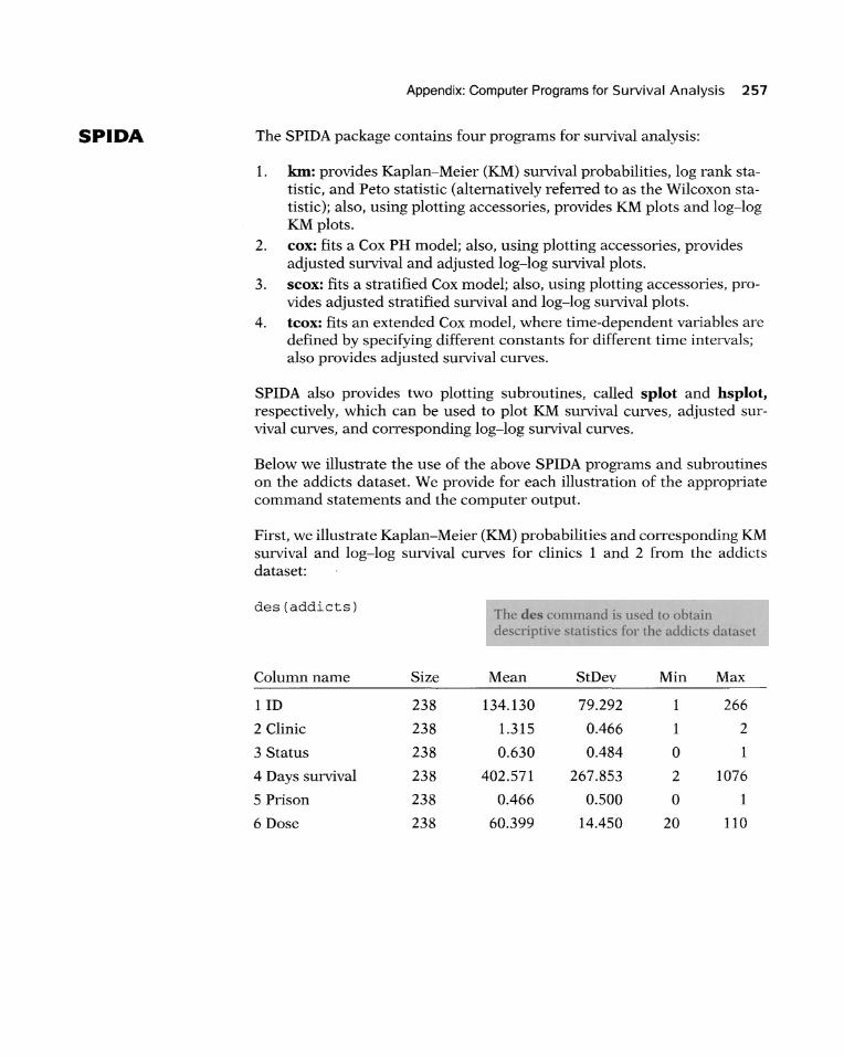
First, we illustrate Kaplan-Meier (KM) probabilities and corresponding KM survival and log-log survival curves for dinics 1 and 2 from the addicts dataset:
des (addicts)
Columnname
lID
2 Clinic
3 Status
4 Days survival
5 Prison
6 Dose
Size
238
238
238
238
238
238
The des commancl i' U
Mean StDev
134.130 79.292
1.315 0.466
0.630 0.484
402.571 267.853
0.466 0.500
60.399 14.450
cl lo obtain clataset
Min Max
1 266
1 2
0
2 1076
0 1
20 110

258 Appendix: Computer Programs for Survival Analysis
Kaplan-Meier (KM) surYival curve are plolted uing splot command. Thc 'c= 1 command cr ale an output file with KM probabilities for each grOlIp.
km (addicts, y=4, s=3, g= 2 ) Th km ommand i u ed LO obtain KM probabililie for the Lwo grollp in the addicts dataset; al 0, logrank and Peto statistic are computed
Group Size
1 163
2 75
%Cen
25.153
62.667
df:l log rank: 27.893
LQ Median UQ
192 428 652
280
p-value: o Peto: 11.078
$sc := km(addicts,y=4,s=3,g=2,sc=1) splot($sc)
1.0 I I I 0.8 1 I I
11 2 I 0.6 1~ 2 I
1~ 2 0.4 1~
I, 0.2 1~
1----, 0.0 1~
0 200 400 600 800
splot($sc , l oglog=l)
10.0
0.95 Med CI
341.000 504
661.000
p-value:O
1000 1200
5.0
Log-log KM slLlyi\'al cun'e are plotted here using splot command wilh loglog= I.
1
0.0
-5.0 -
o 200
1--------------~-,------------
1--
400 600 800 1000 1200
Appendix: Computer Programs for Survival Analysis 259
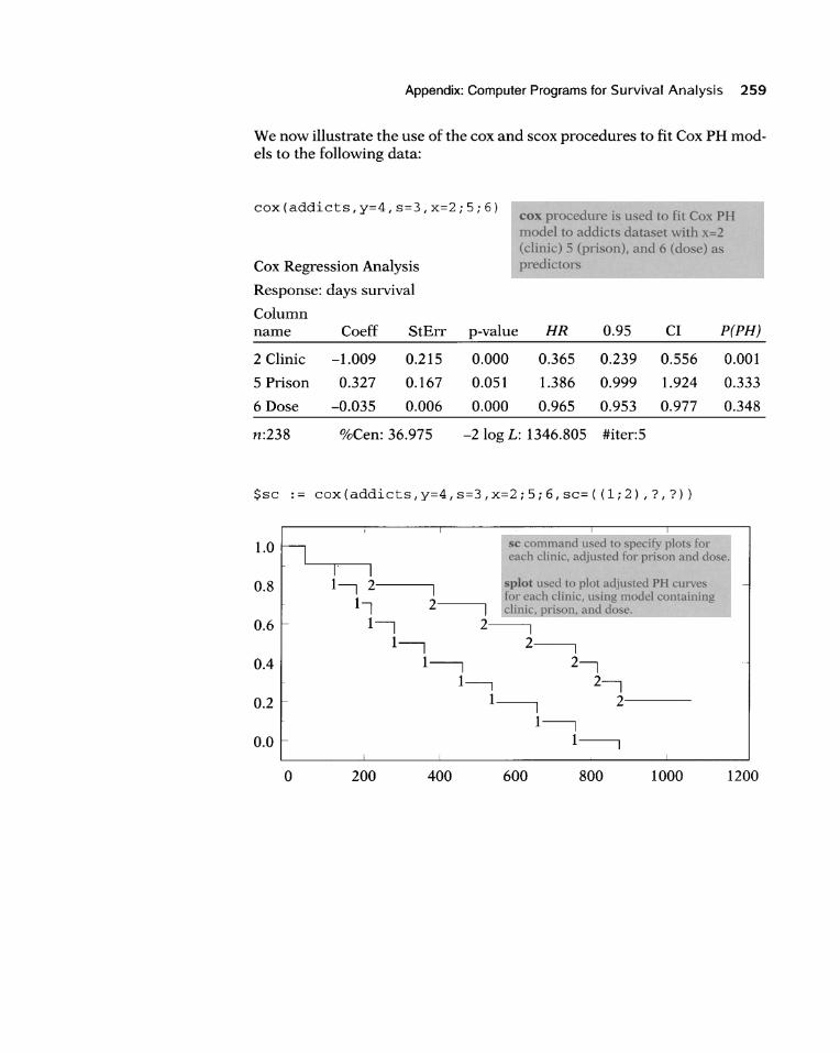
We now illustrate the use of the cox and scox procedures to fit Cox PH models to the following data:
cox(addicts,y=4,s=3,x=2;5 ; 6) cox procedure i u d Lo fiL Cox PH model LO addict data et with x=2 (dink) 5 (prison), and 6 (do e) as predictors Cox Regression Analysis
Response: days survival
Column name Coeff StErr
2 Clinic -1.009 0.215
5 Prison 0.327 0.167
6 Dose -0.035 0.006
n :238 %Cen: 36.975
p-value HR 0.95 CI
0.000 0.365 0.239 0.556
0.051 1.386 0.999 1.924
0.000 0.965 0.953 0.977
-2 log L: 1346.805 #iter:5
$sc . - cox(addicts,y=4,s=3,x=2;5;6,sc=((1;2),?,?))
P(PH)
0.001
0.333
0.348
1.0 sc command used 10 ' pecH)" pi t · for cach dinic, adjulcd for pri on and do e.
0.8 I, 2------, splot used [0 plot adjusted PH curves I for each linie, ulting model containing 1, 2----,1 clinic, prison, and dose.
0.6 1, 2~ 1~ 2~
0.4 1~ 2, 1---, 2,
0.2 1~ 2------1~
0.0 1~
0 200 400 600 800 1000 1200

260 Appendix: Computer Programs for Survival Analysis
$sc := scox(addicts,y=4,s=3,strat=2,x=(5,6),sc=?)
scox pro edure u ed to tratify on cLinic, using pli on and dose a predictors in the model.
Stratified Cox Regression Analysis on Variable: dinic
Response: days survival
Column name Coeff StErr
5 Prison 0.389 0.169
6 Dose -0.035 0.006
n :238 %Cen: 36.975
splot($sc,h=25)
1.0
0.8
0.6
0.4 Clinic 1
0.2
o 200 400
p-value HR 0.95 CI
0.021 1.475 1.059 2.054
0.000 0.965 0.953 0.978
-2 log L: 1195.428 #iter:5
600
plot used to plot tratified cox curve adju ted for prison and do e (in model).
800 1000 1200
We now illustrate the use of the tcox procedure to fit extended Cox models to the data, first using a heavyside function approach with two timedependent variables, and second, using a single time-dependent variable which reflects the continuous diverging appearance of the adjusted survival curves for the two dinics.
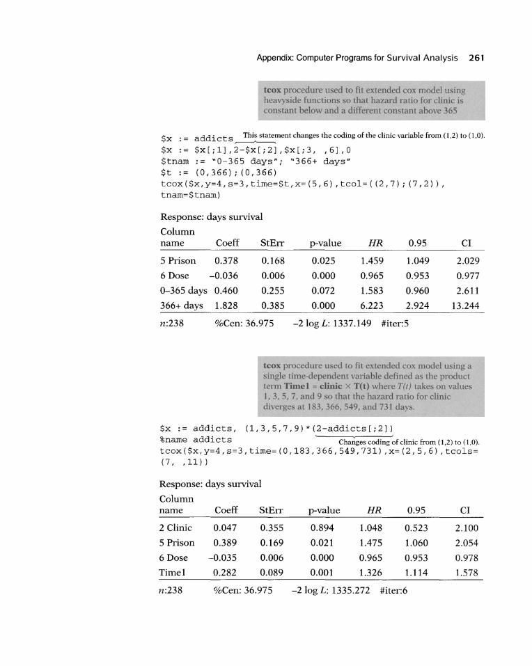
Appendix: Computer Programs for Survival Analysis 261
tcox procedure u ed to fit ext nd d cox model u ing heavy ide funetion 0 lhat hazard ratio for dink i constant below and a different eon tant above 365
$x : = addicts ~ment changes the coding ofthe clinic variable from (1,2) to (1 ,0).
$x:= $x[;1J,2-$x[;2J,$x[;3, ,6],0 $tnarn := "0-365 days"i "366+ days" $t := (0,366) i (0,366)
tcox($x,y=4,s=3,tirne=$t,x=(5,6) ,tco1=((2,7); (7,2)), tnarn=$tnarn)
Response: days survival
Column name Coeff StErr p-value HR 0.95 CI
5 Prison 0.378 0.168 0.025 1.459 1.049 2.029
6 Dose -0.036 0.006 0.000 0.965 0.953 0.977
0-365 days 0.460 0.255 0.072 1.583 0.960 2.611
366+ days 1.828 0.385 0.000 6.223 2.924 13.244
n:238 %Cen: 36.975 -2 log L: 1337.149 #iter:5
tcox proeedure used Lo fit extended cox model u ing a single time-dependent variable defined a the product term Timel = dinic x T(t) wh er T(I) lake' on value 1,3,5, 7, and 9 0 that the hazard ratio for dink diverge at 183,366,549, and 731 days.
$x := addicts, (1,3,5,7,9)*(2-addicts[i 2 ]) %narne addicts Chmi.ges coding of dinic from (1,2) to (1,0). tcOx($x,y=4,s=3,tirne=(0,183,366,549,731),x=(2,5,6),tco1s= (7, ,11))
Response: days survival
Column name Coeff StErr p-value HR 0.95 CI
2 Clinic 0.047 0.355 0.894 1.048 0.523 2.100
5 Prison 0.389 0.169 0.021 1.475 1.060 2.054
6 Dose -0.035 0.006 0.000 0.965 0.953 0.978
Time 1 0.282 0.089 0.001 1.326 1.114 1.578
n:238 %Cen: 36.975 -2 log L: 1335.272 #iter:6
262 Appendix: Computer Programs for Survival Analysis
SAS
SAS EXAMPLE
The SAS package contains three programs for survival analysis:
1. LIFETEST: provides Kaplan-Meier (KM) survival probabilities, log rank statistic, Wilcoxon (i.e., Peto) statistic, KM plots, and log-log KM plots.
2. PHREG: fits a Cox PR model, stratified Cox PH model (using strata statement to identify variables for stratification), and an extended Cox model (using SAS programming statements to define time-dependent variables). Also, PHREG computes predicted survival probabilities for each study subject failure, computes (using a baseline file statement) adjusted survival probabilities for a specified set of predictors, and, using PROC PLOT on an output file, plots adjusted survival and log-log survival probabilities.
3. LIFEREG: fits parametric survival models, in particular, Weibull, log normal, log-logistic and gamma distributions; also, using plotting accessories, provides adjusted survival plots.
Both PHREG and LIFEREG procedures can provide regression diagnostic information in terms of residuals; however, no collinearity diagnostics are provided, even though it is possible to create one's own SAS macro for calculating condition indices and variance decomposition proportions from the inverse of the information matrix derived from the likelihood function. Also, PHREG does not provide a P(PH) statistic for testing the PH assumption.
As we have previously done with the SPIDA package, we now illustrate the use of the SAS survival analysis procedures with the addicts dataset. First, we provide command statements and printout describing the variables in the dataset:
/*
*/
Data file ADDICTS.DAT
Survival times in days of heroin addicts from entry to a clinic until departure.
Data provided by John Caplehorn, c/- The University of Sydney,
Dept of Public Health.
Column 1 2 3 4 5
6
ID of subject clinic (1 or 2) status (O=censored, l=endpoint) survival time (days) prison record? methadone dose (mg/day)

Appendix: Computer Programs for Survival Analysis 263
LIFETEST PRINTOUT
DATA ADDICTS; LABEL ID='SUBJECT ID'
CLINIC='STUDY CLINIC' STATUS='CENSORED=O ' DAYS='SURVIVAL TIME IN DAYS' PRISON='PRISON RECORD (Y/N) ,
1 1 1 2 1 1 3 1 1 4 1 1 5 1 1
261 1 1 26 2 2 1 263 2 0 264 1 1 266 1 1
RUN;
DOSE='METHADONE INPUT ID CLINIC CARDS; 428 0 50 275 1 55 262 0 55 183 0 30 259 1 65
33 1 60 540 0 80 551 0 65
90 0 40 47 0 45
DOSE (mg / DAY) , ; STATUS DAYS PRISON DOSE;
PROC LIFETEST DATA=ADDICTS METHOD=KM PLOTS=(S,LLS); TIME DAYS*STATUS(O); STRATA CLINIC;
RUN;
PROC LIFETEST compute Kaplan-Meier e timate and plot, incJuding log-log plots. AI 0 compute log- rank te t taLi tic.
We now illustrate SAS's PROC LIFETEST by producing Kaplan-Meier survival probabilities and corresponding survival and log-log plots (using PROC PLOT):

264 Appendix: Computer Programs tor Survival Analysis
Product-Limit Survival Estimates
Clinic = 1
Survival standard Number Number
Days Survival Failure error failed left
0.00 1.0000 0 0 0 163
2.00* • • • 0 162
7.00 0.9938 0.00617 0.00615 1 161
17.00 0.9877 0.0123 0.00868 2 160
19.00 0.9815 0.0185 0.0106 3 159
• • • Omitled middl portion or data • • •
840.00* • • • 119 4
857.00 0.0543 0.9457 0.0262 120 3
892.00 0.0362 0.9638 0.0229 121 2
899.00 0.0181 0.9819 0.0172 122 1
905.00* • • • 122 0
*Censored observation.
Quantiles: 75% 652.00 Mean: 431.47
50% 428.00 Standard error: 22.51
25% 192.00
NOTE: The last observation was censored, so the estimate of the mean is biased.
Product-Limit Survival Estimates
Clinic = 2
Days Survival Failure
0.00 1.0000 0
2.00* • •
Survival standard Number Number
error failed left
0 0 75
• 0 74

Appendix: Computer Programs for Survival Analysis 265
Survival standard Number Number
Days Survival Failure error failed left
13.00 0.9865 0.0135 0.0134 1 73
26.00 0.9730 0.0270 0.0189 2 72
35.00 0.9595 0.0405 0.0229 3 71
• • • Omitted middle portion of data • • •
932.00* • • • 28 5
944.00* • • • 28 4
969.00* • • • 28 3
1021.00* • • • 28 2
1052.00* • • • 28 1
1076.00* • • • 28 0
*Censored observation.
Quantiles: 75% • Mean: 629.82
50% • Standard Error: 39.34
25% 280.00
NOTE: The last observation was censored so the estimate of the mean is biased.
Summary of the Number of Censored and Uncensored Values
CLINIC Total Failed Censored %Censored
1 163 122 41 25.1534
2 75 28 47 62.6667
Total 238 150 88 36.974

266 Appendix: Computer Programs for Survival Analysis
LIFETEST PRINTOUT
SURVIVAL FUNCTION ESTIMATES
1.0+ I I I I
0.9+ I I I I
0.8+ I I I I
>' 0.7+ o I
j : >' I o 0.6+ .g I
:9 SDF I ~ I ;a I ca 0.5+
·E : ~ I
I 0.4+
I I I I
*A-B-B AA B
AA B-B AAA BB
AAB AABB-B
AA BB A B AA B-B
AA BB A B-B AA B-B
A BB AAA B-B
AA BB-B A A-A
AAA AA
AA AA
AA
B--B
A-A AA
AAA AA
AA A A AA
AAA AA
Kaplan-Meier Curve
B-B B-----B
B
Legend for Strata Symbols A: Clinic = 1 B: Clinic = 2
0.3+ I
A-A A
I I I
0.2+ I I I I
0.1+ I I I I
0.0+
A-A AAA
A-A AAA
A
AA AA
A-A AA
AA A-A
A A
-+-+-+-+-+-+-+-+-+-+-+-+- - - - - - - - - - - - - - - - - - - - - - - - - - - - - --o 100 200 300 400 500 600 700 800 900 1000 1100
Survival time in days

Appendix: Computer Programs tor Survival Analysis 267
LIFETEST PRlNTOUT
LOG(-LOG(SURVIVAL FUNCTION» ESTIMATES Log-Log Kaplan-Mei r unival curve .
L(-L(S)) I 2+
I I I I I
1+ I I I I I
0+ I I I I I
-1+ I I I I I
-2+ I I I I I
-3+ I I I I I
-4+ I I I I I
-5+ I I I I I
-6+ I
++ A+
+++ BA ++
++ ++
++ A
A
A
AA
A
AA
AA
AA
AA
AA
AA
AA B AA +
AA
AA
AA
A BBB A +B
AAB
AAB+B AAB
A+A B AAA +B
AA B
A+A +B +A +++B+
B+B BB
+BB
*+++
A+
A A
*A Legend for Strata Symbols A: Clinic = 1 B: Clinic = 2
L+_+_+_+_+_+_+_+ _+ _+_+_+_+ _____ ___ __________ ___ _ 1.5 2.0 2.5 3.0 3.5 4~ 4.5 5.0 5.5 6.0 6.5 7~
Logdays

268 Appendix: Computer Programs for Survival Analysis
LIFETEST PRINTOUT
Testing Homogeneity of Survival Curves over Strata
Rank statistics
CLINIC
1
Log-rank
31.09184
-31.0918
Wilcoxon
2
2929
-2929
Covariance Matrix for the Log-Rank Statistics
CLINIC
1
2
34.6579
-34.6579
2
-34.6579
34.6579
Covariance Matrix for the Wilcoxon Statistics
CLINIC
2
1
737868
-737868
2
-737868
737868
Test of Equality over Strata
Test ' Chi-Square DF PR > Chi-Square
Log-rank 27.8927 1 0.0001
Wilcoxon 11 .6268 1 0.0007
-2 log (LR) 26.0236 1 0.0001
PROC MEANS DATA=ADD1CTS NOPR1NT; VAR PR1SON DOSE; OUTPUT OUT=R1SK MEAN=PR1SON DOSE;
RUN;
DATA 1NR1SK; SET R1SK; DO 1=1 TO 2; CL1N1C=1; OUTPUT; END; RUN;
PROC MEA S is used to calculate the overall mean for the pri on and dose variables and the "OUTPUT" laternenl et' up an output file called "RISK" Lo be u ed by PROC PHREG for plolting adju ted ur\'ival and log-log sun i\'al cur\'e .
The dataset "1 RISK" is creaLed rrom Lhe data et "RISK" Lo contain two Iincs of data. one for each clinic. with Lhe overall mean [or pri on and do e on each line.
PROCPRI
PROC PR1NT DATA=1NR1SK; VAR CL1N1C PR1SON DOSE;
RUN;

Appendix: Computer Programs tor Survival Analysis 269
PRINTOUT OF "INRISK"
OBS CLINIC PRISON DOSE
1 2
1
2 0.46639 0.46639
60.3992 60.3992
We now apply PROC PHREG to the addicts dataset to fit Cox PM, stratified Cox, and extended Cox models as described below:
Fit Cox PH model with predictor CLlNIC, PRISO , and DOSE.
PROC PHREG DATA=ADDICTS; MODEL DAYS*STATUS(O)=CLINIC PRISON DOSE / RL; 10 10;
BASELINE COVARIATES=INRISK OUT=MODELl SURVIVAL=Sl / NOMEAN; RUN;
urvival cun:c paralcly for cach dinic.
PROC PLOT DATA=MODEL1; TITLE2 'PLOT OF SURVIVAL FUNCTION VS. TIME'; TITLE3 'ADJUSTED FOR CLINIC, DOSE, AND PRISON'; PLOT Sl*DAYS=CLINIC;
RUN;
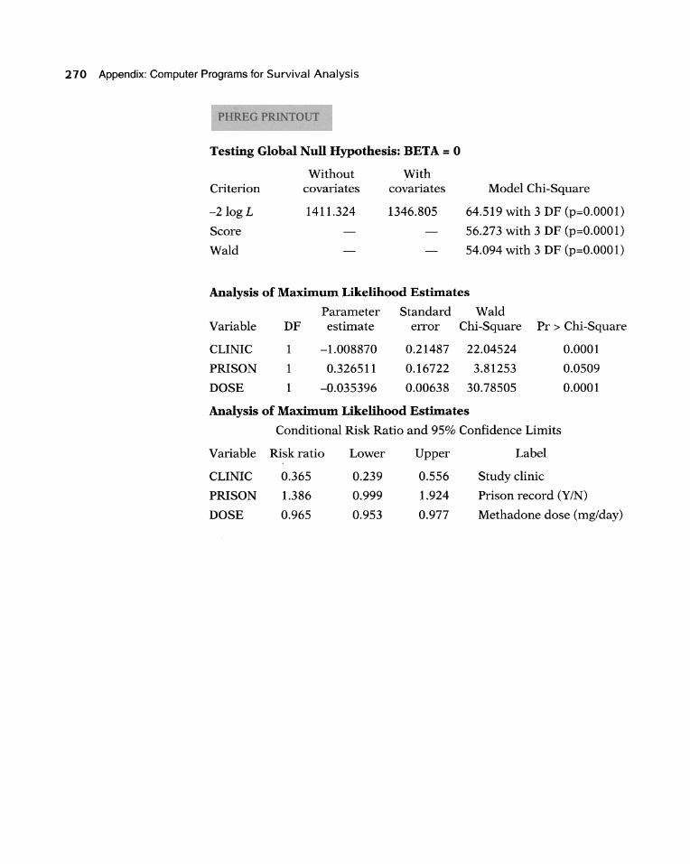
PHREG PRINTOUT
The PHREG Procedure
Dataset: WORK.ADDICTS Dependent Variable: DAYS Censoring Variable: STATUS Censoring Value(s): 0 Ties Handling: BRESLOW
SURVIVAL TIME IN DAYS CENSORED = 0
Summary of the Number of Event and Censored Values
Total Event Censored Percent censored
238 150 88 36.97
270 Appendix: Computer Programs tor Survival Analysis
PHREG PRINTO T
Testing Global Null Hypothesis: BETA = 0
Criterion
-2 log L
Score
Wald
Without With covariates
1411.324
covariates Model Chi-Square
1346.805 64.519 with 3 DF (p=O.OOOl)
56.273 with 3 DF (p=0.0001)
54.094 with 3 DF (p=0.0001)
Analysis of Maximum Likelihood Estimates
Parameter Standard Wald Variable DF estimate eITor Chi-Square Pr> Chi-Square
CLINIC 1 -1.008870 0.21487 22.04524 0.0001
PRISON 1 0.326511 0.16722 3.81253 0.0509
DOSE 1 -0.035396 0.00638 30.78505 0.0001
Analysis of Maximum Likelihood Estimates
Conditional Risk Ratio and 95% Confidence Limits
Variable Risk ratio Lower Upper Label
CLINIC 0.365 0.239 0.556 Study dinic
PRISON 1.386 0.999 1.924 Prison record (Y/N)
DOSE 0.965 0.953 0.977 Methadone dose (mg/day)

Appendix: Computer Programs for Survival Analysis 211
PLOT OF SURVIVAL FUNCTION VS. TIME ADJUSTED FOR CLINIC, DOSE, AND PRISON
Plot of SI *DAYS. Symbol is value of CLINIC.
~ .. . § '" " <=i 0 .~
.a
l ::>
Cf)
1.0 + 112 I 112222 I 11 22222 I 111 222 I 111 222 I 11 222 I 11 2222
~8 + 11 2222 11 222 2
0.6 +
0.4 +
0.2 +
0.0 +
11 11
11 111
11 11
111 11
11
2222 222
1 1 111
111 11
22 2222
2 22 22
22 2 2 2
1 1
11 1 1
11 11
1 1
2 2
11 11
2 2
2
1 1 1
2 2
2
2
11 1
--+------------+------------+------------+------------+------------+--o ~ ~ ~ ~ 1~
Survival time in days
272 Appendix: Computer Programs for Survival Analysis
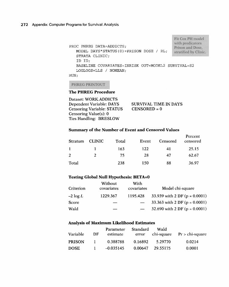
PROC PHREG DATA=ADDICTS;
Fit Co. P mod I with predicators Pd on and 00 e,
MODEL DAYS*STATUS(O)=PRISON DOSE / RL; STRATA CLINIC;
tratified b. Clinie.
ID ID; BASELINE COVARIATES=INRISK OUT=MODEL2 SURVIVAL=S2 LOGLOGS=LLS / NOMEAN;
RUN;
PHREG PR! TO T
The PHREG Procedure
Dataset: WORK.ADDICTS Dependent Variable: DAYS Censoring Variable: STATUS Censoring Value(s): 0 Ties Handling: BRESLOW
SURVIVAL TIME IN DAYS CENSORED = 0
Summary of the Number of Event and Censored Values
Stratum CLINIC
2
Total
1
2
Total
163
75
238
Event
122
28
150
Censored
41
47
88
Percent censored
25.15
62.67
36.97
Testing Global Null Hypothesis: BETA=O
Criterion
-2 log L
Score
Wald
Without With covariates
1229.367
covariates Model chi-square
1195.428 33.939 with 2 DF (p = 0.0001)
33.363 with 2 DF (p = 0.0001)
32.690 with 2 DF (p = 0.0001)
Analysis of Maximum Likelihood Estimates
Parameter Standard Wald Variable DF estimate error chi-square Pr > chi-square
PRISON 0.388788 0.16892 5.29770 0.0214
DOSE -0.035145 0.00647 29.55175 0.0001

PHREG PRI TO T
Appendix: Computer Programs for Survival Analysis 273
Conditional Risk Ratio and 95% Confidence Limits
Variable Risk ratio
PRISON 1.475
DOSE 0.965
DATA MODEL2; SET MODEL2; LOG_T=LOG(DAYS) ;
Lower
1.059
0.953
Upper
2.054
0.978
LABEL LOG_T='LOG OF TIME (DAYS)'; RUN;
PROC PLOT DATA=MODEL2;
Label
Prison record (Y/N)
Methadone dose (mg/day)
Plot-adju ted un'h'al and log-log unival cun'es for PH model wiLh predictor PRISO and DOSE, tratified b CU IC.
TITLE2 'PLOTS OF SURVIVAL FUNCTION AND LOG(-LOG(S)) VS. TIME' ; TITLE3 'ADJUSTED FOR DOSE AND PRISON'; TITLE4 'STRATIFIED BY CLINIC'; PLOT S2*DAYS=CLINIC LLS*LOG_T=CLINIC;
RUN;
PLOT OF SURVIVAL FUNCTION VS. TIME ADJUSTED FOR DOSE AND PRISON STRATIFIED BY CLINIC
Plot of S2*DAYS. Symbol is value of CLINIC.
1.0 + 11
0.8+
0.6+
·1 § ."
] 0.4+
0.2+
0.0+
111 I 1112 I 11122
I 122 1112 1122
11 2 11 1122 11 22 11 22 11 2
11 2 2 111 11 111 11
111 111
11 11
I I 11 I
11 11
I 11
I
11
11 I
o 200 400 600 800 1000
Survival time in days
274 Appendix: Computer Programs for Survival Analysis
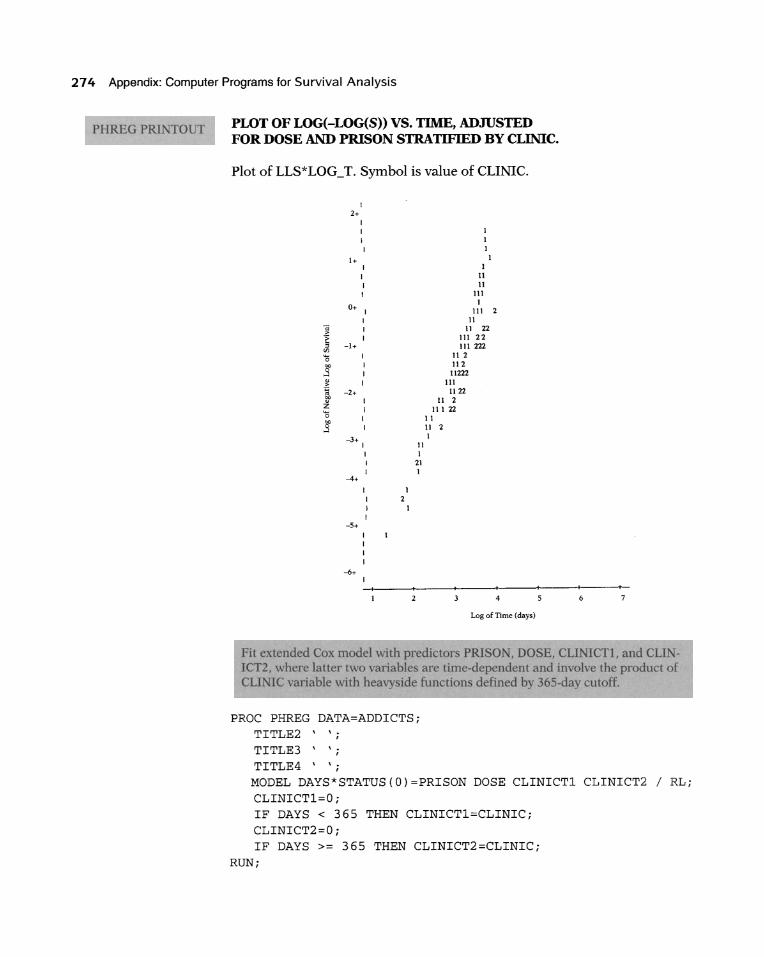
PLOT OF LOG(-LOG(S» VS. TIME, ADJUSTED FOR DOSE AND PRISON STRATIFIED BY CLINIC.
Plot of LLS*LOG_T. Symbol is value of CLINIC.
] ~ ~
</J
'0 .. 0
o-l
.~ 11' Z '0 ~
o-l
2+ I
1+
0+
-1+
-2+
- 3+
-4+
-5+
-6+
I I
I
I
1 2
11 1
21 1
1 1
1 11 11
111 1
111 2 11
11 22 111 22 111 222
112 112
11222 111
1122 11 2
111 22 11 11 2
4
Log ofTime (days)
6
Fit extended Cox model wilh prediclors PRISO ,DOSE, CLINICn, and CLI -ICT2, where latter two variables are time-dependent and involve the producl of CLINIe variable with heavyside functions defined by 36S-day cutoff.
PROC PHREG DATA=ADDICTS; TITLE2 \ \; TITLE3 \ \; TITLE4 \ \;
MODEL DAYS*STATUS(O)=PRISON DOSE CLINICTl CLINICT2 / RL; CLINICT1=O; IF DAYS < 365 THEN CLINICT1=CLINIC ; CLINICT2=O; IF DAYS >= 365 THEN CLINICT2=CLINIC;
RUN;
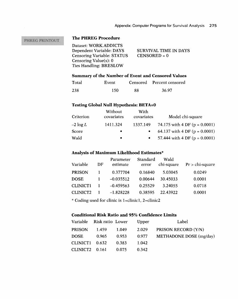
Appendix: Computer Programs for Survival Analysis 275
The PHREG Procedure
Dataset: WORK.ADDICTS Dependent Variable: DAYS Censoring Variable: STATUS Censoring Value(s): 0 Ties Handling: BRESLOW
SURVIVAL TIME IN DAYS CENSORED = 0
Summary of the Number of Event and Censored Values
Total Event Censored Percent censored
238 150 88 36.97
Testing Global Null Hypothesis: BETA=O
Without With Criterion covariates covariates Model chi-square
-2logL 1411.324 1337.149 74.175 with 4 DF (p = 0.0001)
Score • • 64.137 with 4 DF (p = 0.0001)
Wald • • 57.444 with 4 DF (p = 0.0001)
Analysis of Maximum Likelihood Estimates*
Parameter Standard Wald Variable DF estimate error chi-square Pr > chi-square
PRISON 1 0.377704 0.16840 5.03045 0.0249
DOSE 1 -0.035512 0.00644 30.45033 0.0001
CLINICTI 1 -0.459563 0.25529 3.24055 0.0718
CLINICT2 -1.828228 0.38595 22.43922 0.0001
* Coding used for dinic is 1 =dinic1 , 2=dinic2
Conditional Risk Ratio and 95% Confidence Limits
Variable Risk ratio Lower Upper Label
PRISON 1.459 1.049 2.029 PRISON RECORD (Y/N)
DOSE 0.965 0.953 0.977 METHADONE DOSE (mglday)
CLINICTI 0.632 0.383 1.042
CLINICT2 0.161 0.075 0.342

276 Appendix: Computer Programs for Survival Analysis
PROC PHREG DATA=ADDICTS; MODEL DAYS*STATUS(O)=CLINIC PRISON DOSE CLINIC_T / RL COVB; IF O<=DAYS<=183 THEN T=l;
Fit extended Co . model v.'ith predictors CLINIC, PRISO ,DOSE, and a time-dependent CLI IC_T variable defined to allow diverging
IF 183<DAYS<=365 THEN T=3; IF 365<DAYS<=548 THEN T=5; IF 548<DAYS<=730 THEN T=7; IF DAYS>730 THEN T=9; un ival cun'e over time. CLINIC_T=CLINIC*T;
RUN;
The PHREG Procedure
Datset: WORK.ADDICTS Dependent Variable: DAYS Censoring Variable: STATUS Censoring Value(s): 0 Ties Handling: BRESLOW
SURVIVAL TIME IN DAYS CENSORED=O
Summary of the Number of Event and Censored Values
Total Event Censored Percent censored
238 150 88 36.97
Testing Global Null Hypothesis: BETA=O
Without With Criterion covariates covariates Model chi-square
-2 log L 1411.324 1335.518 75.806 with 4 DF (p = 0.0001)
Score • • 66.449 with 4 DF (p = 0.0001)
Wald • • 57.647 with 4 DF (p = 0.0001)
Analysis of Maximum Likelihood Estimates
Parameter Standard Wald Variable DF estimate error chi-square Pr > chi-square
CLINIC 1 0.028900 0.35290 0.00671 0.9347
PRISON 1 0.388220 0.16880 5.28969 0.0215
DOSE 1 -0.035283 0.00644 30.00208 0.0001
CLINIC_T 1 -0.278001 0.08827 9.91870 0.0016

BMDP
BMDP EXAMPLE
Appendix: Computer Programs for Survival Analysis 277
Conditional Risk Ratio and 95% Confidence Limits
Variable Risk ratio Lower Upper Label
CLINIC 1.029 0.515 2.056 STUDY CLINIC
PRISON 1.474 1.059 2.052 PRISON RECORD (Y/N)
DOSE 0.965 0.953 0.978 METRADONE DOSE (mg/DAY)
CLINIC_T 0.757 0.637 0.900
The BMDP paekage eontains two programs for survival analysis;
1. lL: provides Kaplan-Meier (KM) survival probabilities, log-rank statistie (ealled in the program the generalized Savage Mantel-Cox test), generalized Wilcoxon (i .e., Peto) test, KM plots, and log-log KM plots.
2. 2L: fits the Cox PR model, stratified Cox PR model (using a stratification statement in the Iregression paragraph to identify variables for stratifieation), and an extended Cox model (using a function statement to define time-dependent variables) . Also eomputes and plots adjusted survival and log- log survival probabilities for a specified set of predictors.
As with SAS's PROC PRREG, the 2L program also provides regression diagnostie information in terms of residuals; however, no eollinearity diagnostics are provided, even though it is possible to create one's own BMDP maero for calculating eondition indices and varianee deeomposition proportions from the inverse of the information matrix derived from the likelihood function. Also, the 2L program does not provide a GOF statistie for testing the PR assumption.
We now illustrate the use of the BMDP survival analysis proeedures with the addicts dataset. First, we use lL to provide eommand statements and printout for obtaining Kaplan-Meier survival probabilities eorresponding survival eurves:
PROGRAM INSTRUCTIONS / INPUT UNIT IS 11.
VARIABLES = 6. FORMAT = FREE.
/ VARIABLE NAMES = ID, CLINIC, STATUS, DAYS, PRISON, DOSE. / FORM TIME = DAYS.
UNIT = DAYS. STATUS = STATUS.

278 Appendix: Computer Programs for Survival Analysis
RESPONSE = 1. / GROUP CODES (CLINIC) = 1, 2.
NAMES(CLINIC) = CLINIC_l, CLINIC_2. / ESTIMATE METHOD = PRODUCT.
/ END
TIME VARIABLE IS DAYS
PLOTS = SURV, LOG. BROOK = 95. GROUPING = CLINIC. STATISTICS = ALL. EXPECTED.
The e eommand produee tables of KM survival probabilities, log-rank and Peto te t tati tie ,and urvival and log-log survival eurves [or eaeh dinic.
KM probabilitie for Clinie 1.
PRODUCT-LIMIT SURVIVAL ANALYSIS GROUPING VARIABLE IS CLINIC LEVEL IS CLINIC_l
CASE CASE TIME STATUS CUMULATIVE STANDARD LABEL NUMBER DAYS SURVIVAL ERROR
217 2.00 CENSORED 175 7.00 DEAD 0 . 9938 0.0062 164 17.00 DEAD 0 . 9877 0.0087 220 19 . 00 DEAD 0.9815 0.0106 193 28.00 CENSORED 203 28 . 00 CENSÖRED
Omitted middle portion of data
55 857.00 DEAD 0.0543 0.0262 9 892.00 DEAD 0.0362 0.0229
54 899.00 DEAD 0 . 0181 0.0172 70 905.00 CENSORED
MEAN SURVIVAL TIME = 431.57 LIMITED TO 905.00 S.E.
QUANTILE 75TH MEDIAN (50TH) 25TH
ESTIMATE 192.00 428.00 652 . 00
ASYMPTOTIC STANDARD ERROR
15 . 79 48.59 54.25
CUM CUM DEAD LOST
0 0 1 0 2 0 3 0 3 0 3 0
120 0 121 0 122 0 122 0
22.526
BROOKMEYER-CROWLEY 95% CONFIDENCE INTERVAL FOR MEDIAN SURVIVAL TIME (341.00, 504.00)
*** NOTE *** BROOKMEYER-CROWLEY CONFIDENCE INTERVAL ASSUMES NO TIES
REMAIN AT RISK
162 161 160 159 158 157
3
2 1
o
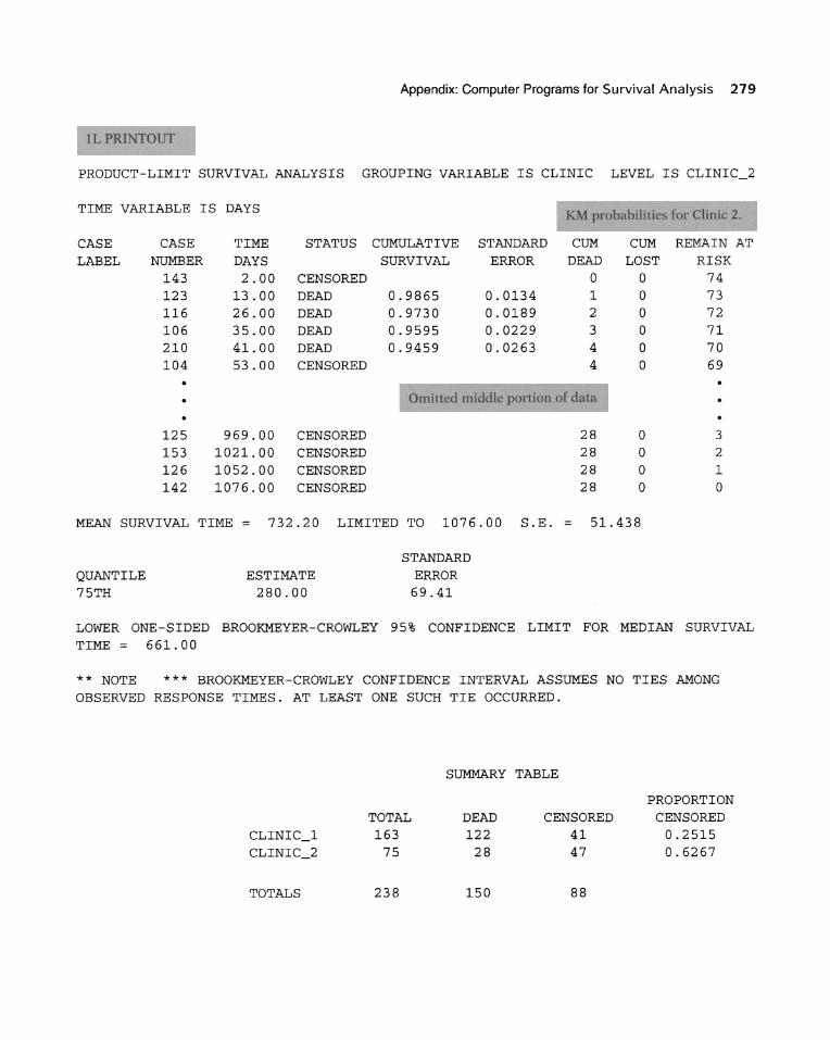
Appendix: Computer Programs for Survival Analysis 279
PRODUCT-LIMIT SURVIVAL ANALYSIS GROUPING VARIABLE IS CLINIC LEVEL IS CLINIC_2
TIME VARIABLE IS DAYS KM probabilitie for Clinic 2.
CASE CASE TIME STATUS CUMULATIVE STANDARD CUM CUM REMAIN AT LABEL NUMBER DAYS SURV I VAL ERROR DEAD LOST RISK
143 123 116 106 210 104
125 153 126 142
MEAN SURVIVAL
QUANTILE 75TH
2.00 CENSORED 0 0 13.00 DEAD 0.9865 0.0134 1 0 26.00 DEAD 0.9730 0 . 0189 2 0 35.00 DEAD 0.9595 0.0229 3 0 41.00 DEAD 0.9459 0 . 0263 4 0 53.00 CENSORED 4 0
Omitted middle portion of data
969.00 CENSORED 28 0 1021. 00 CENSORED 28 0 1052 . 00 CENSORED 28 0 1076.00 CENSORED 28 0
TIME = 732.20 LIMITED TO 1076 . 00 S.E. 51. 438
ESTIMATE 280 . 00
STANDARD ERROR 69.41
74 73 72 71 70 69
3 2 1 0
LOWER ONE-SIDED BROOKMEYER-CROWLEY 95% CONFIDENCE LIMIT FOR MEDIAN SURVIVAL TIME = 661.00
** NOTE *** BROOKMEYER-CROWLEY CONFIDENCE INTERVAL ASSUMES NO TIES AMONG OBSERVED RESPONSE TIMES. AT LEAST ONE SUCH TIE OCCURRED.
SUMMARY TABLE
PROPORTION TOTAL DEAD CENSORED CENSORED
CLINIC_1 163 122 41 0.2515 CLINIC_2 75 28 47 0 . 6267
TOTALS 238 150 88

280 Appendix: Computer Programs for Survival Analysis
CLINIC_l CLINIC_2
CLINIC 1 CLINIC_2
SUMS FOR OBSERVED AND EXPECTED RESPONSES (MANTEL-COX TEST)
CLINIC_l CLINIC_2
OBSERVED 122.0
28.0
EXPECTED 90 . 91 59 . 09
(OBS / EXP) 1. 34 0.47
The "log-rank" tati tic i' called the generalized avage (Manlel-Cox) taU tic in BMDP and lhe "Pelo" lali 'lic i' caUed lh Generalized Wilco on (Bre low) lati tic in BMDP
TEST STATISTICS
STATISTIC D.F . P-VALUE GENERALIZED SAVAGE (MANTEL-COX) 27.895 1 0.0000 TARONE-WARE 17.597 1 0 .0 000 GENERALIZED WILCOXON (BRESLOW) 11. 627 1 0.0007 GENERALIZED WILCOXON (PETO-PRENTICE) 15.652 1 0.0001
PATTERN OF CENSORED DATA
** * ****** * ** * *** ****** **** * * ** * * * * * * * ****** * * *** * ** * ** .+ .... + ... . + .... + .... + .... + ... . + .... + •• .. + .... + .... + .... + .... + .
100. 300 . 500. 700 . 900 . 1100 0 . 00 200. 400. 600 . 800. 1000 1200
PATTERN OF TRUE RESPONSE TIMES
************************************ **** *** * ** ****** **** * ** ** * * * *
.+ .... + .... + .... + .. .. + .. .. + ... . + ... . + ... . + . ... + .. . . + ... . + ... . +. 100. 300. 500 . 700. 900. 1100
0.00 200. 400. 600. 800. 1000 1200
Appendix: Computer Programs for Survival Analysis 281
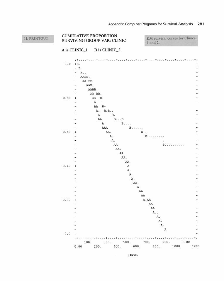
CUMULATIVE PROPORTION SURVIVING GROUP V AR: CLINIC
KM sUIvival curve 1 and 2 .
. + .... + .... + .... + .. . . + .... + .... + .... + . ... + . . . . + .. . . + .. .. + .. .. +. 1.0 +B.
- B. B ..
- AABB.
AA.BB AAB.
AABB. AA BB.
0.80 + AA B. A
AA B-A. B.B ..
A B. AA. B ... B
A B ....
0.60 +
AAA
AA. A.
A.
B ..... .
B ..
B •.....•••
AA AA.
B ..••••••..
0.40 +
0.80 +
0.0 +
AA
AA. AA
A
A. A.
A. AA.
A. AA
AA A.AA
AA AA
A ..
A. A.
A. A
+
+
+
+
+
+
.+ .... + .... + .... + .... + .... + .... + .... + ... . + .... + .... + .... + .... +. 100. 300. 500. 700. 900. 1100
0.00 200. 400. 600. 800. 1000 1200
DAYS

282 Appendix: Computer Programs for Survival Analysis
IL PRINTOUT LOG OF CUMULATIVE PROPORTION SURVIVING GROUP V AR: CLINIC
log- log KM curve for Clinic 1 and 2 .
. + .... + .... + .... + .... + .... + . ... + .... + .... + .... + .... + .... + .... +.
1.0 +
0.9 +BBB .
0.8 + B.BBBBB.
0.7 +
0.6 +
0.5 +
0.4 +
0.3 +
0.2 +
0.1 +
o. +
AAABBBB.
AA. BB.B ..
MA BB . . . B ....
AAAAA B ..... B ..
MA. B ....•.•..
MA. B ......... .
MA
AA
AA
AA
MA.
A. AA
AA
A.A. A.
A. A
A
A ..
A. A
A.
A ..
A
A
+
+ +
+
+
+
+
+
+
+
+
.+ . ... + .... + ... . + .... + .... + .... + .... + ..•. + .... + .... + .... + .... +.
100. 300. 500 . 700. 900. 1100 0.00 200. 400. 600. 800. 1000 1200
DAYS
Appendix: Computer Programs for Survival Analysis 283
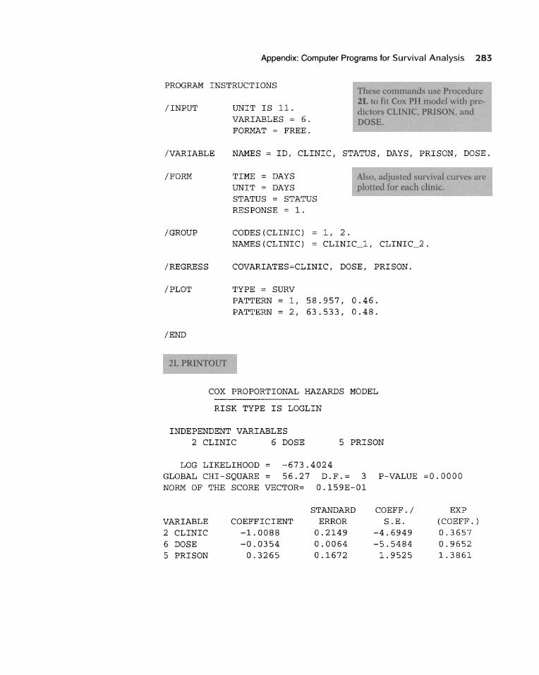
PROGRAM INSTRUCTIONS
/INPUT UNIT IS 11. VARIABLES = 6. FORMAT = FREE.
/VARIABLE NAMES = ID, CLINIC, STATUS, DAYS, PRISON, DOSE.
/FORM
/GROUP
/REGRESS
/PLOT
/END
TIME = DAYS UNIT = DAYS STATUS STATUS RESPONSE = 1.
CODES (CLINIC) NAMES(CLINIC)
1, 2. CLINIC_1, CLINIC_2.
COVARIATES=CLINIC, DOSE, PRISON.
TYPE = SURV PATTERN 1, 58.957, 0.46. PATTERN = 2, 63.533, 0.48.
2L PRINTOUT
COX PROPORTIONAL HAZARDS MODEL
RISK TYPE IS LOGLIN
INDEPENDENT VARIABLES 2 CLINIC 6 DOSE 5 PRISON
LOG LIKELIHOOD -673.4024
are
GLOBAL CHI-SQUARE 56.27 D.F.= 3 P-VALUE =0.0000 NORM OF THE SCORE VECTOR= 0.159E-01
STANDARD COEFF./ EXP VARIABLE COEFFICIENT ERROR S.E. (COEFF. ) 2 CLINIC -1.0088 0.2149 -4.6949 0.3657 6 DOSE -0.0354 0.0064 -5.5484 0.9652 5 PRISON 0.3265 0.1672 1. 9525 1.3861

284 Appendix: Computer Programs for Survival Analysis
Estimated Survivor Function Adju ted urvival curves plotted [or each dinic [or PH mod I ontaining CU IC, PRISO and DOSE variable
.+ ..... + ..... + ... . . + ..... + .. . . . + ..... + ..... + .. ... + ..... + ... . . +.
1.0 +*B - ABB - AA BBBB -
0.90 +
0 .8 0 +
0.70 +
0.60 +
0.50 +
A BB A BB
AA B A BBB
A B AA BBB
AA A
A
A
AA AA
A
AA A
A
AA AA
BBB B
AA AA
A
A
A
A
BBBB BB
BB B
BB BB
BB BB
B
BB BB
B
BB BB
B
B
AM B
B
0.40 +
0.30 +
0.20 +
0 .1 0 +
A
AA AA
A
A
A
AA AM
A
AA AA
A
B
BB BB
AA AA
A
AA AA
AA A
AM
A
+
+
+
+
+
+
+
+
+
0.0 + . + .. .. . + . .. . . + . ... . + ... . . + . .... + ... .. + .... . + .. ... + . . . . . +.
100. 300. 500 . 700. 900 . 0.00 200 . 40 0. 600. 800 . 1000
DAYS

Appendix: Computer Programs tor Survival Analysis 285
/ REGRESS
/ PLOT
/ END
2L PRINTOUT
COVARIATES=DOSE, PRISON. STRATA = CLINIC . TYPE = SURV, LOG. PATTERN = 60.399, 0.466.
COX PROPORTIONAL HAZARDS MODEL
RISK TYPE IS LOGLIN
INDEPENDENT VARIABLES 6 DOSE 5 PRISON
LOG LIKELIHOOD -597.7140 GLOBAL CHI-SQUARE 33.36 D.F.= 2 P-VALUE =0.0000 NORM OF THE SCORE VECTOR= 0.221E-06
VARIABLE 6 DOSE 5 PRISON
COEFFICIENT -0.0351
0.3888
PLOT DIRECTORY CONVERSION
PATTERN 1
FACTOR ** 1. 000
STANDARD ERROR 0.0065 0 . 1689
6
COEFF ./ S.E.
-5.4362 2.3017
EXP (COEFF. ) 0.9655 1.4752
DOSE 60.399
5 PRISON
.466
** USE THE CONVERSION FACTOR AS AN EXPONENT TO CONVERT THE ESTIMATE FOR THE BASELINE SURVIVOR FUNCTION TO THE SURVIVOR FUNCTION FOR A PARTICULAR COVARIATE PATTERN . THE PROPORTIONAL HAZARDS BASELINE SURVIVOR FUNCTION IS PRINTED WHEN YOU REQUEST THE SURVIVAL OPTION IN THE PRINT PARAGRAPH.

286 Appendix: Computer Programs for Survival Analysis
2L PRINTO T tralified Cox model containing PRISO
Estimated Survivor Function
. + ..... + ..... + .... . + . .... + ... . . + . ... . + ..... + ... . . + .. . .. + ... . . +.
1.0 +*
- A* - A*BB
0 . 90 +
0 . 80 +
0 . 70 +
0 . 60 +
0.50 +
0.40 +
0.30 +
A BB A B
AASB
AASB
AAB A BB A B AA BB
A B A BB
AA BB A BBB
AA BBB AA BB
A BBB AM
A
AA A
AA AM
A
BBBBB BBBB
A
AA AA
A
A
A
A
A
A
AM
A
A
AA
BB BB
BBB BBB
BBB
A
0.20 +
0 . 10 +
0.0 +
AM
AA A
AA A
AA A
A
AM
A
+
+
+
+
+
+
+
+
+
+
+
. + ..... + . .... + .. ... + .. ... + ... . . +. " . . + .. . . . + . .... + . . ... + . . . .. + .
100 . 300. 500. 700. 900.
0 . 00 200. 400. 600 . 800. 1000
DAYS
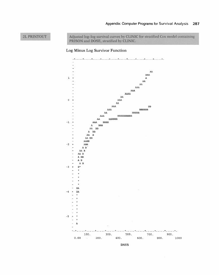
Appendix: Computer Programs for Survival Analysis 287
Lralined Cox model containing
Log Minus Log Survivor Function
. + ..... + ..•.. + ..... + ..... + ..... + ....• + ..... + ..... + ..... + ..... +.
1 +
o + AA
AAA AA
AAA AAA
AA
AA
AAA A
AA
AA
AAA AAA
AAAA
BBBBBB BBBBB
BB
AAA BBBBBBBBBB AA BBBBBB
-1 + AAA BBBB A BBB
AA BB
A BB AA B
AA BB
AABB
-2 + ABB
AB'
AAB
AAB
A BB AB
AB
-3 + B*
- BA
-4 + BA
-5 + * - * - A
-. + ..... + ..... + ..... + ..... + ..... + ..... + ..... + ..... + ..... + ..... +.
100. 300. 500. 700. 900. 0.00 200. 400. 600. 800. 1000
DAYS

288 Appendix: Computer Programs for Survival Analysis
Fit extended Cox model with predictor PRI 0 ,DOSE, CU ICT), and CU -ICT2, wherc latter tw variable are tirne-dependenl and defined by the FUNC-TIO laternent a eparate product of the CUNIC variable \dth hea"yside functions defined b. 365-day cutofL
PROGRAM INSTRUCTIONS
/ REGRESS
/ FUNCTION
COVARIATES=DOSE, PRISON. ADD = CLINICT1, CLINICT2. AUXILIARY = CLINIC, DAYS .
CLINICT1 O. CLINICT2 O. IF (DAYS < 365) THEN CLINICT1=CLINIC. IF (DAYS >= 365) THEN CLINICT2=CLINIC .
/ END
2LPRI TO T
COX PROPORTIONAL HAZARDS MODEL
RISK TYPE IS LOGLIN
INDEPENDENT VARIABLES 6 DOSE 5 PRISON 7 CLINICT1 8 CLINICT2
LOG LIKELIHOOD -668.5774 GLOBAL CHI-SQUARE 64.14 D.F.= 4 P-VALUE =0.0000 NORM OF THE SCORE VECTOR= 0.1433E-04
STANDARD COEFF. / EXP VARIABLE COEFFICIENT ERROR S.E. (COEFF. ) 6 DOSE -0.0355 0.0064 -5.5182 0.9651 5 PRISON 0.3777 0.1684 2 . 2429 1.4589 7 CLINICT1 -0.4596 0.2553 -1. 8002 0.6316 8 CLINICT2 -1.8282 0.3859 -4.7370 0.1607
Appendix: Computer Programs for Survival Analysis 289
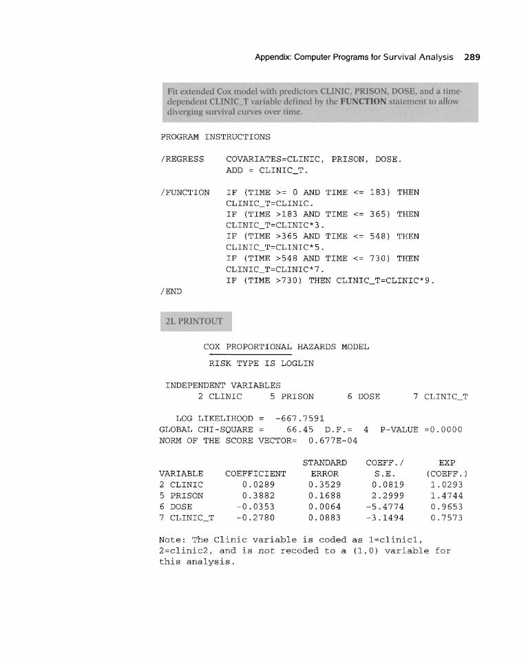
Fit xtended Cox model with predictor CLINIC, PRISO ,DOSE, and a timedependent CL! leT variable defined b. the FU CTION -tal ment LO allO\\' di erging 'urvival curve over time.
PROGRAM INSTRUCTIONS
/REGRESS COVARIATES=CLINIC, PRISON, DOSE. ADD = CLINIC_T.
/FUNCTION IF (TIME >= o AND TIME <= 183) THEN CLINIC_T=CLINIC. IF (TIME >183 AND TIME <= 365) THEN CLINIC_T=CLINIC*3. IF (TIME >365 AND TIME <= 548) THEN CLINIC_T=CLINIC*5. IF (TIME >548 AND TIME <= 730 ) THEN CLINIC_T=CLINIC*7. IF (TIME >730) THEN CLINIC_T=CLINIC*9.
/END
2L PRI TOUT
COX PROPORTIONAL HAZARDS MODEL
RISK TYPE IS LOGLIN
INDEPENDENT VARIABLES 2 CLINIC 5 PRISON 6 DOSE
LOG LIKELIHOOD -667.7591 GLOBAL CHI-SQUARE 66.45 D.F.= 4 P-VALUE =0.0000 NORM OF THE SCORE VECTOR= 0.677E-04
STANDARD COEFF./ EXP VARIABLE COEFFICIENT ERROR S.E. (COEFF. ) 2 CLINIC 0.0289 0.3529 0.0819 1.0293 5 PRISON 0.3882 0.1688 2.2999 1.4744 6 DOSE -0.0353 0.0064 -5.4774 0.9653 7 CLINIC T -0.2780 0.0883 -3.1494 0.7573 -
Note: The Clinic variable is coded as 1=clinic1, 2=clinic2, and is not recoded to a (1,0) variable for this analysis.
Appendix: Datasets
In this appendix, we provide listings of datasets that are illustrated in the textbook using examples of computer output either as part of a chapter's main presentation or as part of the practice exercises or test. A table of contents for this appendix is given as follows:
Dataset Name Pages
ADDICTS.DAT 292
ANDERSON.DAT 295
CHEMO.DAT 296
STAN.DAT 297
VETS.DAT 301
291
292 Appendix: Datasets
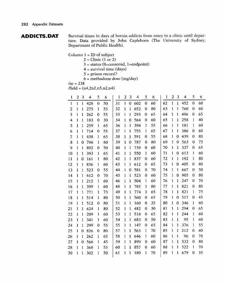
ADDICTS.DAT Survival tirnes in days of heroin addicts frorn entry to a dinic until departure. Data provided by lohn Caplehom (The University of Sydney, Departrnent of Public Health).
Colurnn 1 == ID of subject 2 == Clinic (1 or 2) 3 == status (O==censored, l==endpoint) 4 == survival time (days) 5 == prison record? 6 == rnethadone dose (rng/day)
Im == 238 lfield == (n4,2n2,n5,n2,n4)
1 2 3 4 5 6
1 1 1 428 0 50 2 1 1 275 1 55 3 1 1 262 0 55 4 1 1 183 0 30 5 1 1 259 1 65 6 1 1 714 0 55 7 1 1 438 1 65 8 1 0 796 1 60 9 1 1 892 0 50
10 1 1 393 1 65 11 1 0 161 1 80 12 1 1 836 1 60 13 1 1 523 0 55 14 1 1 612 0 70 15 1 1 212 1 60 16 1 1 399 1 60 17 1 1 771 1 75 18 1 1 514 1 80 19 1 1 512 0 80 21 1 1 624 1 80 22 1 1 209 1 60 23 1 1 341 1 60 24 1 1 299 0 55 25 1 0 826 0 80 26 1 1 262 1 65 27 1 0 566 1 45 28 1 1 368 1 55 30 1 1 302 1 50
1 2 3 4 5 6
31 1 0 602 0 60 32 1 1 652 0 80 33 1 1 293 0 65 34 1 0 564 0 60 36 1 1 394 1 55
37 1 1 755 1 65 38 1 1 591 0 55 39 1 0 787 0 80 40 1 1 739 0 60 41 1 1 550 1 60 42 1 1 837 0 60 43 1 1 612 0 65 44 1 0 581 0 70 45 1 1 523 0 60 46 1 1 504 1 60 48 1 1 785 1 80 49 1 1 774 1 65 50 1 1 560 0 65 51 1 1 160 0 35 52 1 1 482 0 30 53 1 1 518 0 65 54 1 1 683 0 50 55 1 1 147 0 65 57 1 1 563 1 70 58 1 1 646 1 60 59 1 1 899 0 60 60 1 1 857 0 60 61 1 1 180 1 70
1 2 3 4 5 6
62 1 1 452 0 60 63 1 1 760 0 60 64 1 1 496 0 65 65 1 1 258 1 40 66 1 1 181 1 60 67 1 1 386 0 60 68 1 0 439 0 80 69 1 0 563 0 75 70 1 1 337 0 65 71 1 0 613 1 60 72 1 1 192 1 80 73 1 0 405 0 80 74 1 1 667 0 50 75 1 0 905 0 80 76 1 1 247 0 70 77 1 1 821 0 80 78 1 1 821 1 75 79 1 0 517 0 45 80 1 0 346 1 60 81 1 1 294 0 65 82 1 1 244 1 60 83 1 1 95 1 60 84 1 1 376 1 55 85 1 1 212 0 40 86 1 1 96 0 70 87 1 1 532 0 80 88 1 1 522 1 70 89 1 1 679 0 35

1 2 3 4 5 6
90 1 0 408 0 50 91 1 0 840 0 80 92 1 0 148 1 65 93 1 1 168 0 65 94 1 1 489 0 80 95 1 0 541 0 80 96 1 1 205 0 50 97 1 0 475 1 75 98 1 1 237 0 45 99 1 1 517 0 70
100 1 1 749 0 70 101 1 150 1 80 102 1 1 465 0 65 103 2 1 708 1 60 104 2 0 713 0 50 105 2 0 146 0 50 106 2 1 450 0 55 109 2 0 555 0 80 110 2 1 460 0 50 111 2 0 53 1 60 113 2 1 122 1 60 114 2 1 35 1 40 118 2 0 532 0 70 119 2 0 684 0 65 120 2 0 769 1 70 121 2 0 591 0 70 122 2 0 769 1 40 123 2 0 609 1 100 124 2 0 932 1 80 125 2 0 932 1 80 126 2 0 587 0 110 127 2 1 26 0 40 128 2 0 72 1 40 129 2 0 641 0 70 131 2 0 367 0 70 132 2 0 633 0 70 133 2 1 661 0 40
1 2 3 4 5 6
134 2 1 232 1 70 135 2 1 13 1 60 137 2 0 563 0 70 138 2 0 969 0 80 143 2 01052 0 80 144 2 0 944 1 80 145 2 0 881 0 80 146 2 190 1 50 148 2 1 79 0 40 149 2 0 884 1 50 150 2 1 170 0 40 153 2 1 286 0 45 156 2 0 358 0 60 158 2 0 326 1 60 159 2 0 769 1 40 160 2 1 161 0 40 161 2 0 564 1 80 162 2 1 268 1 70 163 2 0 611 1 40 164 2 1 322 0 55 165 2 01076 1 80 166 2 0 2 1 40 168 2 0 788 0 70 169 2 0 575 0 80 170 2 1 109 1 70 171 2 0 730 1 80 172 2 0 790 0 90 173 2 0 456 1 70 175 2 1 231 1 60 176 2 1 143 1 70 177 2 0 86 1 40 178201021080 179 2 0 684 1 80 180 2 1 878 1 60 181 2 1 216 0 100 182 2 0 808 0 60 183 2 1 268 1 40
ADDICTS.DAT 293
1 2 3 4 5 6
184 2 0 222 0 40 186 2 0 683 0 100 187 2 0 496 0 40 188 2 1 389 0 55 189 1 1 126 75 190 1 1 17 1 40 192 1 1 350 0 60 193 2 0 531 1 65 194 1 0 317 1 50 195 1 0 461 1 75 196 1 1 37 0 60 197 1 1 167 1 55 198 1 1 358 0 45 199 1 1 49 0 60 200 1 1 457 1 40 201 1 1 127 0 20 202 1 1 7 1 40 203 1 1 29 1 60 204 1 1 62 0 40 205 1 0 150 1 60 206 1 1 223 1 40 207 1 0 129 1 40 208 1 0 204 1 65 209 1 1 129 1 50 210 1 1 581 0 65 211 1 1 176 0 55 212 1 1 30 0 60 213 1 1 41 0 60 214 1 0 543 0 40 215 1 0 210 1 50 216 1 1 193 1 70 217 1 1 44 0 55 218 1 1 367 0 45 219 1 1 348 1 60 220 1 0 28 0 50 221 1 0 337 0 40 222 1 0 175 1 60

294 Appendix: Datasets
1 2 3 4 5 6 1 2 3 4 5 6 1 2 3 4 5 6
223 2 1 149 1 80 238 2 0 531 1 45 252 1 1 180 1 60 224 1 1 546 1 50 239 1 0 98 0 40 253 1 1 314 0 70 225 1 1 84 0 45 240 1 1 145 1 55 254 1 0 480 0 50 226 1 0 283 1 80 241 1 1 50 0 50 255 1 0 325 1 60 227 1 1 533 0 55 242 1 0 53 0 50 256 2 1 280 0 90 228 1 1 207 1 50 243 1 0 103 1 50 257 1 1 204 0 50 229 1 1 216 0 50 244 1 0 2 1 60 258 2 1 366 0 55 230 1 0 28 0 50 245 1 1 157 1 60 259 2 0 531 1 50 231 1 1 67 1 50 246 1 1 75 1 55 260 1 1 59 1 45 232 1 0 62 1 60 247 1 1 19 1 40 261 1 1 33 1 60 233 1 0 111 0 55 248 1 1 35 0 60 262 2 1 540 0 80 234 1 1 257 1 60 249 2 0 394 1 80 263 2 0 551 0 65 235 1 1 136 1 55 250 1 1 117 0 40 264 1 1 90 0 40 236 1 0 342 0 60 251 1 1 175 1 60 266 1 1 47 0 45 237 2 1 41 0 40

ANDERSONDAT 295
ANDERSON.DAT Survival times in weeks (in remission) of 42 leukemia patients in clinical trial to compare treatment with placebo. Data from Freireich et al., "The effect of 6-mercaptopurine on the duration of steroid-induced remissions in acute leukemia," Blood 21,699-716,1963.
Column 1 = survival time (weeks) 2 = status (0 = censored, 1 = relapse) 3 = sex (1 = male, 0 = female) 4 = 10gWBC 5 = Rx (1 = placebo, 0 = treatment)
/nr = 42 /field = (n3,2n2,n5,n2)
1 2 3 4 5 1 2 3 4 5 1 2 3 4 5
35 0 1 1.45 0 9 0 0 2.80 0 8 1 0 3.52 1
34 0 1 1.47 0 7 1 0 4.43 0 8 1 0 3.05 1
32 0 1 2.20 0 6 0 0 3.20 0 8 1 0 2.32
32 0 1 2.53 0 6 1 0 2.31 0 8 1 1 3.26 1
25 0 1 1.78 0 6 1 1 4.06 0 5 1 1 3.49 1
23 1 1 2.57 0 6 1 0 3.28 0 5 1 0 3.97 1
22 1 1 2.32 0 23 1 1 1.97 1 4 1 1 4.36 1
20 0 1 2.01 0 22 1 0 2.73 1 4 1 1 2.42 1
19 0 0 2.05 0 17 1 0 2.95 1 3 1 1 4.01 1
17 0 0 2.16 0 15 1 0 2.30 1 2 1 1 4.91 1
16 1 1 3.60 0 12 1 0 1.50 1 2 1 1 4.48 1
13 1 0 2.88 0 12 1 0 3.06 1 1 1 1 2.80 1
11 0 0 2.60 0 11 1 0 3.49 1 1 1 1 5.00 1
10 0 0 2.70 0 11 1 0 2.12 1
10 1 0 2.96 0

296 Appendix: Datasets
CHEMO.DAT Survival times in days from a dinical trial on gastric carcinoma, involving 90 patients randomized to either chemotherapy alone or to a combination of chemotherapy and radiation. Data from Stablein et al., "The analysis of survival data with nonproportional hazard functions," COl1trolled Clil1ical Trials 2, 149-159, 1981.
Column 1 = Rx (1 = chemotherapy, 2 = chemotherapy and radiation) 2 = status (0 = censored, 1 = died) 3 = survival time (days)
Inr = 3 lfield = (sl,el5)
1 2 3 1 2 3 1 2 3 1 2 3 1 2
1 1 17 1 1 197 1 0 882 2 1 301 2 1 1 1 42 1 1 208 1 0 892 2 1 342 2 1
1 1 44 1 1 234 1 0 1031 2 1 354 2 1
1 1 48 1 1 235 1 0 1033 2 1 356 2 1
1 1 60 1 1 254 1 0 1306 2 1 358 2 1 1 1 72 1 1 307 1 0 1335 2 1 380 2 1
1 1 74 1 1 315 1 1 1366 2 0 381 2 1
1 1 95 1 1 401 1 0 1452 2 1 383 2 1
1 1 103 1 1 445 1 0 1472 2 1 383 2 1
1 1 108 1 1 464 2 1 1 2 1 388 2 0 1 1 122 1 1 484 2 1 63 2 1 394 2 1
1 1 144 1 1 528 2 1 105 2 1 408 2 1
1 1 167 1 1 542 2 1 129 2 1 460 2 0 1 1 170 1 1 567 2 1 182 2 1 489 2 1
1 1 183 1 1 577 2 1 216 2 1 499 2 1
1 1 185 1 1 580 2 1 250 2 1 524 2 0
1 1 193 1 1 795 2 1 262 2 0 529 2 0
1 1 195 1 1 855 2 1 301 2 1 535 2 0
1 1 197 1 0 882 2 1 301 2 1 562 2 0
3
535 562 675 676 748 748 778 786 797 945 955 968
1180 1245 1271 1277 1397 1512 1519

STANFDAT 297
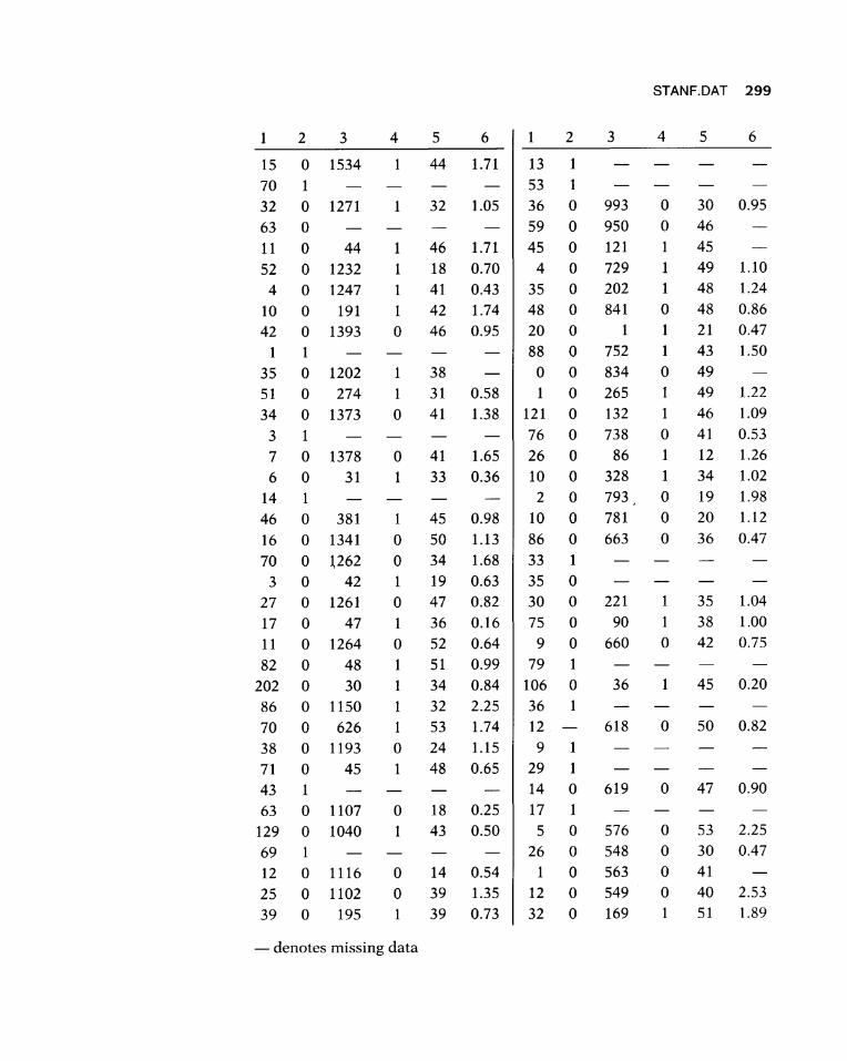
STANF.DAT Survival times in days for 249 patients in Stanford Heart Transplant Trial. Data from Kalbfleisch, J., and Prentice, R., The Statistical Analysis of Failure Time Data, John Wiley and Sons, New York, 1980.
Column 1 = pretransplant survival time 2 = status at first endpoint (0 = alive, 1 = dead) 3 = posttransplant survival time 4 = status at second endpoint (Feb 1980) 5 = age at transplant 6 = tissue mismatch score
/field = (n3,n2,sl,n4,n2,n3,sl,n4)
1 2 3 4 5 6 1 2 3 4 5 6
49 1 70 0 1 1 54 0.47
5 1 34 1
0 0 15 1 54 1.11 15 0 836 1 44 1.58
35 0 3 1 40 1.66 15 1
17 1 16 0 60 1 64 0.69
2 1 50 0 1996 1 49 0.91
50 0 623 1 51 1.32 22 0 3694 0 40 0.38
39 1 11 1
84 1 45 0 54 1 49 2.09
11 0 46 1 42 0.61 18 0 47 1 62 0.87
25 0 126 1 48 0.36 4 0 0 1 41 0.87
7 1 1 0 51 1 50
16 0 64 1 54 1.89 40 0 2878 1 49 0.75
36 0 1350 1 54 0.87 57 0 3410 1 45 0.98
0 1 2 1
27 0 279 1 49 1.12 1 1
35 1 39 1
19 0 23 1 56 2.05 0 0 44 1 36 0.00
36 1 1 0 994 1 48 0.81
17 0 10 1 56 2.76 20 0 51 1 47 1.38
7 0 1024 1 43 1.13 8 1
11 0 39 1 42 1.38 35 0 1478 1 36 1.35
2 0 730 1 58 0.96 82 0 897 1 46
82 0 136 1 52 1.62 31 0 254 1 48 1.08
24 0 1961 1 33 1.06 101 1
112 0 40 0 148 1 47
262 1 2 1
- denotes missing data

298 Appendix: Datasets
1 2 3
9 0 51 66 0 3021
148 1 20 77
2 1
57 26 32 11 31
56 2
9 4
30 3
o 323 o 2984
o 66 1
o o 2723 o 550 o 66 1
o 227 o 65 o 2805 o 25 o 2734 o 631
26 0 63 12 4 0
1 1 45 0 2474 20 1
209 0 547 66 0 29 25 0 1384
5 0 544 31 0 48 36 0 297
4 1 7 0 1318
59 0 50 30 0 1352
138 0 68 159 0 26 340 1
4 5 6 1 2 3
1 52 1.51 309 0 146 o 38 0.98 27 0 431
1
o 1
o 1 1
1
1
o 1
o 1
48 32 49
32 48 51
19 45 48
53 47 26
1.82 0.19 0.66
1.93 0.12 1.12
1.02 1.68 1.20 1.68 0.97 1.46
1 56 2.16 1 29 0.61
1 52 1.70
1 49 0.81
1 53 1.08 1 46 1.41 1 52 1.94 1 53 3.05 1 42 0.60
1
1 1
1 1
48 1.44 46 2.25 54 0.68 51 1.33 52 0.82
4 0 161 1
12 20
95 20 37 56 50 70
1
5 29
1
1
10
o 14
o 2313 o 1634 o 48
1 o 2127 o 263 o 2106 1
o 293 o 2025 o 2000 o 2006 o 1995 o 1945
6 0 65 2 0 731
40 0 1866 18 0 538 o 0 1846
26 0 68 19 0 1778 68 0 928 55 1 11 0 1722
1 0 1718 30 0 22 29 0 7 25 0 40 47 0 1612 46 0 25
1 0 1638 59 0 1547
- denotes missing data
4 5 6
1 45 0.16 1 47 0.33 1 43 1.20 1
o 1 1
1
1
o
1
o o o o o
40 26 23 28
35 49 40
43 30 45 15 47
38
0.46 1.78 0.77
0.67 0.48 0.86
0.70 1.44 1.46 1.26
1.65 1.28
1 55 0.69 1 38 0.42 o 49 0.51 1 49 2.76 o 44 0.83 1 35 0.85 o 27 0.70 1 50 1.12
o 40 0.95 o 39 1.77 1
1
1
o 1
o o
27 1.64 28 1.00 42 1.59 51 1.25 52 0.53 48 0.43 50 0.18
STANF.DAT 299
12345612 3 4 5 6 ------------------------
15 0 1534 1 44 1.71 13 1 70 1
32 0 1271 63 0 11 52
4
10 42
1 35 51 34
3 7 6
o 44 o 1232 o 1247 o 191 o 1393 1 o 1202 o 274 o 1373 1 o 1378 o 31
14 1
46 0 381 16 0 1341 70 0 ~262
3 0 42 27 0 1261 17 0 47 11 0 1264 82 0 48
202 0 30 86 0 1150 70 0 626 38 0 1193 71 0 45 43 1 63 0 1107
129 0 1040 69 1 12 0 1116 25 0 1102 39 0 195
53 1 1 32 1.05 36 0 993
59 0 950
1 1 1
1 o
1 1
o
o 1
46 18 41 42 46
38 31 41
41 33
1.71 45 0 0.70 4 0 0.43 35 0 1.74 48 0 0.95 20 0
88 0 o 0
0.58 1 0 1.38 121 0
76 0 1.65 26 0 0.36 10 0
121 729 202 841
1 752 834 265 132 738
86 328
2 0 793
1 45 0.98 10 0 781 o 50 1.13 86 0 663 o 34 1.68 33 1 1 19 0.63 35 0 o 47 0.82 30 0 221
1 36 0.16 75 0 90 o 52 0.64 9 0 660 1 51 0.99 79 1 1 34 0.84 106 0 36 1 32 2.25 36 1 1 53 1.74 12 618 o 24 1.15 9 1 1 48 0.65 29 1
14 0 619 o 18 0.25 17 1
1 43 0.50 5 0 576 26 0 548
o 14 0.54 1 0 563 o 39 1.35 12 0 549 1 39 0.73 32 0 169
- denotes missing data
o 30 0.95 o 46 1 1 1
o 1 1 o 1
1 o 1 1
45 49 48 48 21 43 49 49 46 41 12 34
1.10 1.24 0.86 0.47 1.50
1.22 1.09 0.53 1.26 1.02
o 19 1.98 o 20 1.12 o 36 0.47
1 35 1.04 1 38 1.00 o 42 0.75
1 45 0.20
o 50 0.82
o 47 0.90
o 53 2.25 o 30 0.47 o 41 o 40 2.53 1 51 1.89

300 Appendix: Datasets
1 2 3 4 5 6 1 2 3 4 5 6
33 0 122 1 51 1.33 89 0 22 1 45 19 0 534 0 20 223 0 8 0 541 0 47 0.43 59 0 231 1 52
16 1 65 0 188 1 52 18 1 82 0 149 0 21 62 0 464 0 38 2.07 27 0 176 0 29 1.72 2 1 192 0
82 0 10 1 13 1.49 67 0 119 0 20 1 1 18 1
70 0 136 1 55 176 0 167 0 322 0 36 1.73 9 0 138 1 41 52 0 5 1 20 11 1 15 0 382 1 36 146 0 9 0 468 0 24 1.39 125 0
63 0 406 0 39 1.18 15 0 107 0 46 15 1 23 0 98 0 19 2 0 391 0 27 1.17 31 1
13 1 30 0 89 0 27 11 0 374 0 47 22 0 56 0 27 92 0 292 1 43 1.40 24 1 17 0 50 1 50 0.50 10 0 60 0 13 36 0 139 1 51 0.96 25 0 2 0 39
117 0 145 1 50 0.96 14 0 51 0 278 1 41 0.98 12 0 1 0 27 18 1
- denotes missing data

VETSDAT 301
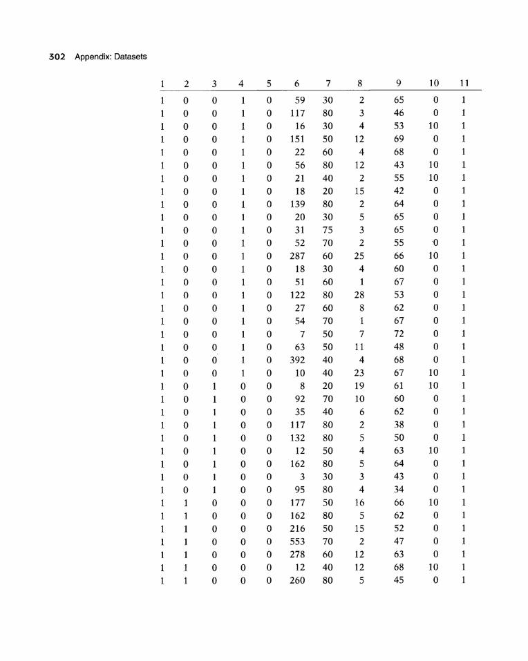
VETS.DAT Survival data for 137 patients from Veteran's Administration Lung Cancer Trial. Data from Kalbfleisch, J., and Prentice, R., The Statistical Analysis of Failure Time Data, John Wiley and Sons, New York, 1980.
Column 1 = treatment (1 = standard, 2 = test) 2 = cell type 1 (1 = large, 0 = other) 3 = cell type 2 (1 = adeno, 0 = other) 4 = cell type 3 (1 = small, 0 = other) 5 = cell type 4 (1 = squamous, 0 = other) 6 = survival time (days) 7 = performance status (0 = worst, ... , 100 = best) 8 = disease duration (months) 9 = age (years)
10 = prior therapy (0 = none, 10 = some) 11 = status (0 = censored, 1 = Died)
/field = (n2, 4nl, N4, 4N3, N2)
1 2 3 4 5 6 7 8 9 10 11
1 0 0 0 1 72 60 7 69 0 1
1 0 0 0 1 411 70 5 64 10 1
1 0 0 0 1 228 60 3 38 0 1
1 0 0 0 1 126 60 9 63 10 1
1 0 0 0 1 118 70 11 65 10 1
1 0 0 0 1 10 20 5 49 0 1
1 0 0 0 1 82 40 10 69 10 1
1 0 0 0 1 110 80 29 68 0 1
1 0 0 0 1 314 50 18 43 0 1
1 0 0 0 1 100 70 6 70 0 0
1 0 0 0 1 42 60 4 81 0 1
1 0 0 0 1 8 40 58 63 10 1
1 0 0 0 1 144 30 4 63 0 1
1 0 0 0 1 25 80 9 52 10 0
1 0 0 0 1 11 70 11 48 10 1
1 0 0 1 0 30 60 3 61 0 1
1 0 0 1 0 384 60 9 42 0 1
1 0 0 1 0 4 40 2 35 0 1
1 0 0 1 0 54 80 4 63 10 1
1 0 0 1 0 13 60 4 56 0
1 0 0 1 0 123 40 3 55 0 0
1 0 0 1 0 97 60 5 67 0 0
1 0 0 1 0 153 60 14 63 10 1
302 Appendix: Datasets
1 2
1 0 1 0 1 0 1 0 1 0 1 0 1 0 1 0 1 0 1 0 1 0 1 0 1 0 1 0 1 0 1 0 1 0 1 0 1 0 1 0 1 0 1 0 1 0 1 0 1 0 1 0 1 0 1 0 1 0 1 0 1 0 1 1 1 1 1 1 1 1 1 1 1 1 1 1
3
o o o o o o o o o o o o o o o o o o o o o o 1 1 1 1 1 1 1 1 1 o o o o o o o
4 5 6 7 8
1 0 59 30 2 1 0 117 80 3 1 0 16 30 4 1 0 151 50 12 1 0 22 60 4 1 0 56 80 12
1 0 21 40 2 1 0 18 20 15 1 0 139 80 2 1 0 20 30 5 1 0 31 75 3
1 0 52 70 2 1 0 287 60 25 1 0 18 30 4 1 0 51 60 1 1 0 122 80 28
1 0 27 60 8 1 0 54 70 1
1 0 7 50 7 1 0 63 50 11 1 0 392 40 4 1 0 10 40 23 o 0 8 20 19 o 0 92 70 10 o 0 35 40 6 o 0 117 80 2 o 0 132 80 5 o 0 12 50 4 o 0 162 80 5 o 0 3 30 3 o 0 95 80 4
o 0 177 50 16 o 0 162 80 5 o 0 216 50 15 o 0 553 70 2 o 0 278 60 12 o 0 12 40 12 o 0 260 80 5
9
65 46 53 69 68 43
55 42 64
65 65
55 66 60 67 53 62 67 72 48 68 67 61 60 62 38
50 63 64 43 34 66 62 52 47 63 68 45
10
o o
10
o o
10
10 o o o o o
10 o o o o o o o o
10 10 o o o o
10 o o o
10 o o o o
10 o
11
1 1 1 1 1 1 1 1 1 1 1 1 1 1 1 1 1
1 1 1 1 1 1 1 1 1 1 1 1 1 1 1 1 1 1 1 1
1

1 2
1 1 1 1 1 1 1 1 1 1 1 1 1 1 1 1 2 0 2 0
2 0 2 0 2 0 2 0 2 0 2 0
2 0 2 0
2 0 2 0 2 0 2 0
2 0
2 0 2 0 2 0 2 0
2 0 2 0
2 0 2 0 2 0
2 0 2 0
2 0 2 0 2 0
2 0
3
o o o o o o o o o o o o o o o o o o o o o o o o o o o o o o o o o o o o o o
4 5 6 7
o 0 200 80 o 0 156 70 o 0 182 90 o 0 143 90 o 0 105 80 o 0 103 80 o 0 250 70 o 0 100 60 o 1 999 90 o 1 112 80 o 1 87 80 o 1 231 50 o 1 242 50 o 1 991 70 o 1 111 70 o 1 1 20 o 1 587 60 o 1 389 90 o 1 33 30 o 1 25 20 o 1 357 70 o 1 467 90 o 1 201 80 o 1 1 50 o 1 30 70 o 1 44 60 o 1 283 90 o 1 15 50 1 0 25 30 1 0 103 70 1 0 21 20 1 0 13 30 1 0 87 60 1 0 2 40 1 0 20 30 1 0 7 20 1 0 24 60 1 0 99 70
8
12 2 2
8 11 5 8
13
12
6
3 8 1 7
3 21
3 2
6 36 13
2 28
7 11
13
2
13
2 22
4
2 2
36 9
11 8 3
9
41 66 62 60
66 38 53 37 54 60 48 52 70
50 62 65 58 62 64 63 58 64 52 35 63 70 51 40 69 36 71 62
60 44 54 66 49 72
VETSDAT 303
10
10 o o o o o
10 10 10 o o
10 o
10 o
10 o o o o o o
10 o o
10 o
10 o
10 o o o
10 10 o o o
11
1 1
o 1
1 1 1
1 1 1 o o 1 1 1 1 1 1
1 1
1 1 1 1 1 1 1 1 1
o 1 1 1 1 1 1 1 1

304 Appendix: Datasets
1 2
2 0 2 0
2 0
2 0 2 0 2 0 2 0 2 0 2 0 2 0 2 0 2 0 2 0 2 0 2 0 2 0 2 0 2 0 2 0 2 0 2 0 2 0 2 0 2 0 2 0 2 0 2 1
2 1 2 1 2 1
2 1 2 1
2 1 2 1
2 1 2 1 2 1 2 1
3
o o o o o o o o 1
1
1
1
1
1
1
1
1 1
1
1. 1 1
1
1
1 1
o o o o o o o o o o o o
4 5 6 7
1 0 8 80 1 0 99 85 1 0 61 70 1 0 25 70 1 0 95 70 1 0 80 50 1 0 51 30 1 0 29 40 o 0 24 40 o 0 18 40 o 0 83 99 o 0 31 80 o 0 51 60 o 0 90 60 o 0 52 60 o 0 73 60 o 0 8 50 o 0 36 70
o 0 48 10 o 0 7 40 o 0 140 70 o 0 186 90 o 0 84 80 o 0 19 50 o 0 45 40 o 0 80 40 o 0 52 60 o 0 164 70 o 0 19 30 o 0 53 60 o 0 15 30 o 0 43 60 o 0 340 80 o 0 133 75 o 0 111 60 o 0 231 70 o 0 378 80 o 0 49 30
8
2
4 2
2
1 17 87
8 2
5 3 3 5
22
3 3 5
8 4
4
3 3 4
10
3 4
4 15 4
12 5
11
10 1
5 18 4
3
9
68 62 71
70 61 71
59 67 60 69 57 39 62
50 43 70
66 61 81 58 63 60 62 42 69 63 45 68 39 66 63 49 64 65 64 67 65 37
10
o o o o o o
10
o o
10 o o o
10 o o o o o o o o
10 o o o o
10 10 o o
10 10 o o
10
o o
11
1
1
1
1
1
1
1
1 1
1
o
1
1
1
1
1
1
1
1
1
1
1
1
1
1
1
1
1
1
1
1
1 1
1
1
1
1

Test Answers
305

306 Test Answers
Chapter 1 True-False Questions:
1. T 2. T 3. T 4. F: step function. 5. F: ranges between 0 and 1. 6. T 7. T 8. T 9. T
10. F: median survival time is longer for group 1 than for group 2. 11. F: six weeks or greater. 12. F: the risk set at 7 weeks contains 15 persons. 13. F: hazard ratio 14. T 15. T
16. h(l) gives the instantaneous potential per unit time for the event to occur given that the individual has survived up to time t; h(t) is greater than or equal to 0; h(t) has no upper bound.
17. Hazard functions
• give insight about conditional failure rates; • help to identify specific model forms (e.g., exponential, Weibull); • are used to specify mathematical models for survival analysis.
18. Three goals of survival analysis are the following: • to estimate and interpret survivor andJor hazard functions; • to compare survivor andJor hazard functions; • to assess the relationship of explanatory variables to survival time.
19.
t(j) m(j) q(j) R(t(j))
Group 1: 0 0 0 25 persons survive ~ 0 years 1.8 1 0 25 persons survive ~ 1.8 years 2.2 1 0 24 persons survive ~ 2.2 years 2.5 1 0 23 persons survive ~ 2.5 years 2.6 1 0 22 persons survive ~ 2.6 years 3.0 1 0 21 persons survive ~ 3.0 years 3.5 1 0 20 persons survive ~ 3.5 years 3.8 1 0 19 persons survive ~ 3.8 years
Chapter 2
Test Answers 307
t(j) m(j) q(j) R(t(j)
5.3 1 0 18 persons survive;?: 5.3 years
5.4 1 0 17 persons survive;?: 5.4 years
5.7 1 0 16 persons survive;?: 5.7 years
6.6 1 0 15 persons survive;?: 6.6 years
8.2 1 0 14 persons survive;?: 8.2 years
8.7 1 0 13 persons survive;?: 8.7 years
9.2 2 0 12 persons survive ;?: 9.2 years
9.8 1 0 10 persons survive;?: 9.8 years
10.0 1 0 9 persons survive ;?: 10.0 years
10.2 1 0 8 persons survive ;?: 10.2 years
10.7 1 0 7 persons survive;?: 10.7 years
11.0 1 0 6 persons survive ;?: 11.0 years
11.1 1 0 5 persons survive ;?: 11.1 years
11.7 1 3 4 persons survive ;?: 11.7 years
20. a. Group 1 has better survival prognosis than group 2 because group 1 has a higher average survival time and a correspondingly lower average hazard rate than group 2.
b. The average survival time and average hazard rates give overall descriptive statistics. The survivor curves allow one to make comparisons over time.
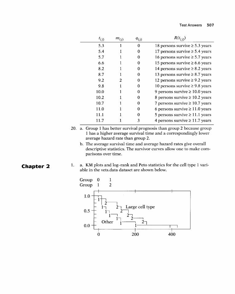
1. a. KM plots and log-rank and Peto statistics for the cell type 1 variable in the vets.data dataset are shown below.
Group 0 1 Group 1 2
1.0
2~ 1, 2, Large cell type
0.5 1--, 21 1~ 2r
1, 2-----, Other 1 I 2,
0.0 1
0 200 400
308 Test Answers
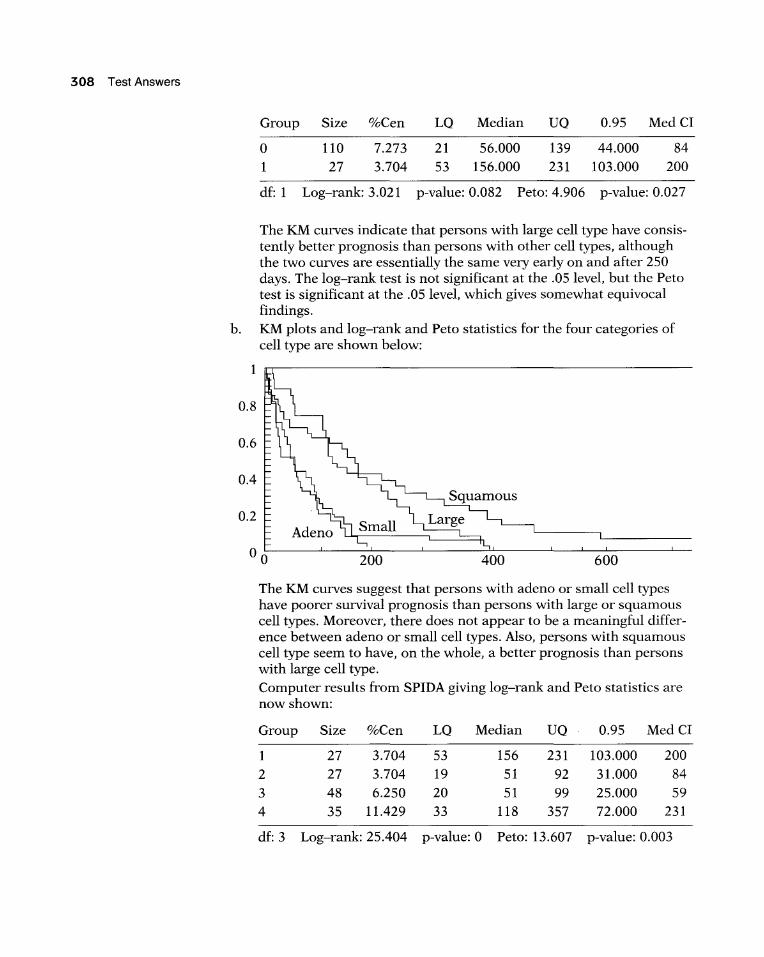
Group Size %Cen La Median va 0.95 Med CI
o 110 7.273 21 56.000 139 44.000 84 1 27 3.704 53 156.000 231 103.000 200
df: 1 Log-rank: 3.021 p-value: 0.082 Peto: 4.906 p-value: 0.027
The KM curves indicate that persons with large cell type have consistently better prognosis than persons with other cell types, although the two curves are essentially the same very early on and after 250 days. The log-rank test is not significant at the .05 level, but the Peto test is significant at the .05 level, which gives somewhat equivocal findings.
b. KM plots and log-rank and Peto statistics for the four categories of cell type are shown below:
1
0.8
0.6
0.4
0.2
600
The KM curves suggest that persons with ade no or small cell types have poorer survival prognosis than persons with large or squamous cell types. Moreover, there does not appear to be a meaningful difference between adeno or small cell types. Also, persons with squamous cell type seem to have, on the whole, a better prognosis than persons with large cell type. Computer results from SPIDA giving log-rank and Peto statistics are nowshown:
Group Size %Cen La Median va 0.95 MedCI
1 27 3.704 53 156 231 103.000 200
2 27 3.704 19 51 92 31.000 84
3 48 6.250 20 51 99 25.000 59
4 35 11.429 33 118 357 72.000 231
df: 3 Log-rank: 25.404 p-value: 0 Peto: 13.607 p-value: 0.003

Test Answers 309
Both the log-rank test and the Peto test yield highly significant p-values, indicating that there is some overall difference between all four curves; that is, the null hypothesis that the four curves have a common survival curve is rejected.
2. a. KM plots for the two dinics are shown below. These plots indicate that patients in dinic 2 have consistently better prognosis for remaining under treatment than do patients in dinic 1. Moreover, it appears that the difference between the two dinics is small before one year of follow-up but diverges after one year of follow-up.
1
0.8
0.6
0.4
0.2
00
b.
Clinic 2
300 600 900
The log-rank statistic (27.893) and Peto statistic (11.078) are both significant well-below the .01 level, indicating that the survival curves for the two dinics are significantly different. The log-rank statistic is nevertheless much larger than the Peto statistic, which makes sense since the log-rank statistic emphasizes the later survival experience, where the two survival curves are far apart, whereas the Peto statistic emphasizes earlier survival experience, where the two survival curves are doser together.
c. If methadone dose is categorized into high (70+), medium (55-70) and low «55), we obtain the KM curves shown below.
310 Test Answers
Chapter 3
300 500 900
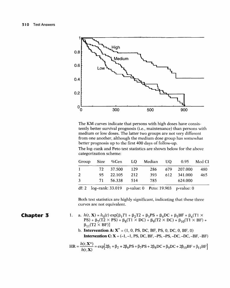
The KM curves indicate that persons with high doses have consistently hetter survival prognosis (i.e., maintenance) than persons with medium or low doses. The latter two groups are not very different from one another, although the medium dose group has somewhat hetter prognosis up to the first 400 days of follow-up.
The log-rank and Peto test statistics are shown helow for the ahove categorization scheme:
Group Size %Cen LQ Median VQ 0.95 MedCI
1 72 37.500 129 286 679 207.000 480 2 95 22.105 212 393 612 341.000 465 3 71 56.338 514 785 624.000
df:2 log-rank: 33.019 p-value: 0 Peto: 19.903 p-value: 0
Both test statistics are highly significant, indicating that these three curves are not equivalent.
1. a. h(t, X) = ho(t) exp[ß1T1 + ß2T2 + ß3PS + ß4DC + ßsBF + ß6(Tl X
PS) + ß7(T2 X PS) + ßs(T1 X DC) + ß9(T2 X DC) + ß lO(Tl X BF) + ßll (T2 X BF)]
h. Intervention A: X* = (1, 0, PS, DC, BF, PS, 0, DC, 0, BF, 0) Intervention C: X = (-1, -1, PS, DC, BF, -PS,-PS, -DC,-DC,-BF, -BF)
~~ [ ] HR = = exp 2ßl + ßz + 2ß6PS + ß7PS + 2ßsDC + ß9DC + 2ßIOBF + ß11BF h(t,X)
Test Answers 311
c. Ho: ß6 = ß7 = ßs = ß9 = ß lO = ß11 = 0 in the full model. Likelihood ratio test statistic: -2 In LR - (-2 In LF), which is approximately x~ under Ho, where R denotes the reduced model (containing no product terms) under Ho, and F denotes the full model (given in part 1a above)
d. The two models being compared are:
e.
Full model (F): h(t, X) = ho(t) exp[ßl Tl + ß2 T2 + ß3PS + ß4DC + ßsBF] Reduced model (R): h(t, X) = ho(t) exp[ß3PS + ß4DC + ßsBF] Ho: ß1 = ß2 = 0 in the full model Likelihood ratio test statistic: -2 In LR - (-2 In LF), which is approximately X~ under Ho
In . A SA( X) [~_( )]exP[ßl+(PS)ß3+(DC)ß4+(BF)ßs] terventlon : t, = '-'\) t
Intervention B: S(t,X) = [So (t)rp [ß2 +(PS)ß3 +(DC)ß4 +(BF)ßs]
Intervention C: S(t,X) = [So(t)rp[-ßI-ß2 +(PS)ß3 +(DC)ß4 +(BF)ßs]
2. a. h(t, X) = ho(t) exp[ßl CHR + ß2 AGE + ß3 (CHR X AGE)] b. Ho: ß3 = 0
LR statistic = 264.90 - 264.69 = 0.21; x2 with 1 dJ. under Ho; not significant. Wald statistic gives a chi-square value of .01, also not significant. Conclusions about interaction: the model should not contain an interaction term.
c. When AGE is controlled (using the gold standard model 2), the hazard ratio for the effect of CHR is exp(.8051) = 2.24, whereas when AGE is not controlled, the hazard ratio for the effect of CHR (using modell) is exp(.8595) = 2.36. Thus, the hazard ratios are not appreciably different, so AGE is not a confounder. Regarding precision, the 95% confidence interval for the effect of CHR in the gold standard model (model 2) is given by exp[.8051 ±
1.96(.3252)] = (1.183, 4.23l) whereas the corresponding 95% confidence interval in the model without AGE (model 1) is given by exp[.8595 ± 1.96(.3116)] = (1.282, 4.350). Both confidence intervals have about the same width, with the latter interval being slightly wider. Thus, controlling for AGE has little effect on the final point and interval estimates of interest.
312 Test Answers
d. If the hazard functions cross for the two levels of the CHR variable, this would mean that none of the models provided are appropriate, because each model assumes that the proportional hazards assumption is met for each predictor in the model. If hazard functions cross for CHR, however, the proportional hazards assumption cannot be satisfied for this variable.
e. For CHR = 1: S(t, X) = [So(t)]exp[O.80S1 +~8S6(AGE)]
For CHR = 0: Set, X) = [SO(t)]exp[O.08S6(AGE)]
f. Using model 1, which is the best model, there is evidence of a moderate effect of CHR on survival time, because the hazard ratio is about 204 with a 95% confidence interval between 1.3 and 404, and the Wald test for significance of this variable is significant below the .01 level.
3. a. Full model (F = model 1): h(t, X) = ho(t) exp [ßl-R.x + ß3 Sex + ß4 log WBC + ßs(Rx X Sex) + ß7(Rx X log WBC)] Reduced model (R = model 4): h(t, X) = ho(t) exp [ßIRx + ß3 Sex + ß4 log WBC]
Ho: ß4 = ßs = 0 LR statistic = 144.218 -139.029 = 5.19; X2 with 2 dJ. under Ho; not significant at 0.05, though significant at 0.10. The chunk test indicates some (though mild) evidence of interaction.
b. Using either a Wald test (P = .776) or a LR test, the product term Rx X log WBC is clearly not significant, and thus should be dropped from modell. Thus, model 2 is preferred to modell.
c. Using model 2, the hazard ratio for the effect of Rx is given by:
HR= ~t,X*) =exp[OA05+2.013 Sex] (t,X) ___
d. Males (Sex = 0): HR = exp[OA05] = 1.499. Females (Sex = 1): HR = exp[OA05 + 2.013(1)] = 11.223.
e. Model 2 is preferred to model 3 if one decides that the coefficients for the variables Rx and Rx X Sex are meaningfully different for the two models. It appears that such corresponding coefficients (00405 vs 0.587 and 2.013 vs. 1.906) are different. The estimated hazard ratios for model 3 are 1.799 (males) and 12.098 (females), which are different, but not very different from the estimates computed in part 3d for model 2. If it is decided that there is a meaningful difference here, then we would conclude that log WBC is a confounder; otherwise log WBC is not a confounder. Note that the log WBC variable is significant in model 2 (P = .000), but this addresses precision and not confounding. When in doubt, as in this case, the safest thing to do (for validity reasons) is to control forlog WBC.

Chapter 4
Test Answers 313
f. Model 2 appears to be best, because there is significant interaction of Rx X Sex (P = .023) and because log WBC is a likely confounder (from part e).
g. The P(PH) values for the sex variable and for the Rx x Sex variable are significant, suggesting that the PR assumption is not satisfied for the sex variable. This indicates that the previous condusions (in 3e and 30 may be inappropriate, and that it may be necessary to carry out an alternative (e.g., stratified) analysis that does not indude the Sex variable in a Cox PH model.
1. The P(PH) values in the printout provide GOF statistics for each variable adjusted for the other variables in the model. These P(PH) values indicate that the dinic variable does not satisfy the PH assumption (P « .01), whereas the prison and dose variables satisfy the PH assumption (P > .10).
2. The log-log plots shown are parallel. However, the reason why they are parallel is because the dinic variable has been induded in the model, because log-log curves for any variable in a PH model must always be parallel. If, instead, the dinic variable had been stratified (i.e., not induded in the model), then the log-log plots comparing the two dinics adjusted for the prison and dose variables might not be parallel.
3. The log-log plots obtained when the dinic variable is stratified (Le., using a.stratified Cox PR model) are not parallel. They intersect early on in follow-up and diverge from each other later in follow-up. These plots therefore indicate that the PR assumption is not satisfied for the dinic variable.
4. Both graphs of log-log plots for the prison variable show curves that intersect and then diverge from one another and then intersect again. Thus, the plots on each graph appear to be quite nonparallel, indicating that the PR assumption is not satisfied for the prison variable. Note, however, that on each graph, the plots are quite dose to one another, so that one might condude that, allowing for random variation, the two plots are essentially coincident; with this latter point of view, one would condude that the PR assumption is satisfied for the prison variable.
5. The conclusion of nonparallellog-Iog plots in question 4 gives a different result about the PR assumption for the prison variable than determined from the GOF tests provided in question 1. That is, the log-log plots suggest that the prison variable does not satisfy the PH assumption, whereas the GOF test suggests that the prison variable satisfies the assumption. Note, however, if the point of view is taken that the two plots are dose enough to suggest coincidence, the graphi-

314 Test Answers
cal conclusion would be the same as the GOF conclusion. Although the final decision is somewhat equivocal here, we prefer to conclude that the PH assumption is satisfied for the prison variable because this is strongly indicated trom the GOF test and questionably counterindicated by the log-log curves.
6. Because maximum methadone dose is a continuous variable, we must categorize this variable into two or more groups in order to graphically evaluate whether it satisfies the PH assumption. Assume that we have categorized this variable into two groups, say low versus high. Then, observed survival plots can be obtained as KM curves for low and high groups separately. To obtain expected plots, we can fit a Cox model containing the dose variable and then substitute suitably chosen values for dose into the formula for the estimated survival curve. Typically, the values substituted would be either the mean or median (maximum) dose in each group. After obtaining observed and expected plots for low and high dose groups, we would conclude that the PH assumption is satisfied if corresponding observed and expected plots are not widely discrepant trom one another. If a noticeable discrepancy is found for at least one pair of observed versus expected plots, we conclude that the PH assumption is not satisfied.
7. h(t, X) = ho(t) exp [ß1(clinic) + ß2(prison) + ß3(dose) + 81(clinic) X g(t) + 82(prison) X g(t) + 8idose) X g(t)
where g(t) is some function of time. The null hypothesis is given by Ho: 81 = 82 = 83 = 0. The test statistic is a likelihood ratio statistic of the form LR = -2 In LR - (-2 In LF)
where R denotes the reduced (PH) model obtained when all B's are 0, and F denotes the full model given above. Under Ho, the LR statistic is approximately chi-square with 3 d.f.
8. Drawbacks of the extended Cox model approach: • not always clear how to specify g(t); different choices may give dif
ferent conclusions; • different modeling strategies to choose trom, e.g., might consider
g(t) to be a polynomial in t and do a backward elimination to eliminate nonsignificant higher-order terms; altematively, might consider g(t) to be linear in t without evaluating higher-order terms. Different strategies may yield different conclusions.
9. h(t, X) = ho(t) exp [ß1(clinic) + ßiprison) + ßidose) + B1(clinic) X g(t)] where g(t) is some function of time. The null hypotmesis is given by Ho: 81 = 0, and the test statistic is either a Wald statistic or a likelihood ratio statistic; either statistic is approximately chi-square with 1 d.f. under the null hypothesis.

Chapter 5
10. t> 365 days: HR = exp[ß1 + SI]
t::; 365 days: HR = exp[ß1]
Test Answers 315
If SI is not equal to zero, then the model does not satisfy the PH assumption for the dinic variable. Thus, a test of Ho: SI = 0 evaluates the PH assumption; a significant result would indicate that the PH assumption is violated. Note that if SI is not equal to zero, then the model assumes that the hazard ratio is not constant over time by giving a different hazard ratio value depending on whether t is greater than 365 days or t is less than or equal to 365 days.
1. By fitting a stratified Cox (SC) model that stratifies on dinic, we can compare adjusted survival curves for each dinic, adjusted for the prison and dose variables. This will allow us to visually describe the extent of dinic differences on survival over time. However, a drawback to stratifying on dinic is that it will not be possible to obtain an estimate of the hazard ratio for the effect of dinic, because dinic will not be induded in the model.
2. The adjusted survival curves indicate that dinic 2 has better survival prognosis than dinic 1 consistently over time. Moreover, it seems that the difference between the effects of dinic 2 and dinic 1 increases over time.
3. hit, X) = h Og(t)exp[ß 1prison + ßzdose], g = 1,2. This is a no-interaction model because the regression coefficients for prison and dose are the same for each stratum.
4. Effect of prison, adjusted for dose: ifR = 1.475,95% CI: (1.059, 2.054). It appears that having a prison record gives a 1.475 increased hazard for failure than does not having a prison record. The p-value is 0.021, which is significant at the 0.05 level.
5. Version 1: hit, X) = ho/t)exp[ß lgprison + ßZgdose], g = 1,2. Version 2: hit, X) = hOg(t)exp[ß1prison + ßzdose + ß3(dinic X prison) + ßidinic X dose)], g = 1,2
6. g = 1 (dinic 1): h1 (t, X) = hOl (t)exp[(0.502)prison + (-0.036)dose] g = 2 (dinic 2): hit, X) = hoit)exp[-0.083)prison + (-0.037)dose]
7. The adjusted survival curves stratified by dinic are virtually identical for the no-interaction and interaction models. Consequently, both graphs (no-interaction versus interaction) indicate the same condusion that dinic 2 has consistently larger survival (i.e., retention) probabilities than dinic 1 as time increases.
8. Ho: ß3 = ß4 = 0 in the versio1l2 model (~e., the no-interaction assumption is satisfied). LR = -2 In LR - (-2 In Lp ) where R denotes the reduced (no-interaction) model and F denotes the full (interaction) model. Under the null hypothesis, LR is approximately a chi-square with 2 degrees of freedom.

316 Test Answers
Chapter 6
Computed LR = 1195.428 - 1193.558 = 1.87; P = 0.395; thus, the null hypothesis is not rejected and we conclude that the no-interaction model is preferable to the interaction model.
1. For the chemo data, the -log-log KM curves intersect at around 600 days; thus the curves are not parallel, and this suggests that the treatment variable does not satisfy the PH assumption.
2. The P(PH) value for the Tx variable is 0, indicating that the PH assumption is not satisfied for the treatment variable based on this goodness-of-fit test.
3. h(t, X) = ho(t)exp[ßl (Tx)gl (t) + ßzCTx)gzCt) + ßiTx)git )] where
g (t) = { 1 if 0 ::; t < 250 days 1 0 if otherwise
gzCt) = { 1 if 250 ::; t < 500 days o if otherwise
g (t) = { 1 if t ~ 500 days 3 0 if otherwise
4. Based on the printout the hazard ratio estimates and corresponding p-values and 95% confidence intervals are given as follows for each time interval:
HazRatio p-value 0.95 CI
o ::; t < 250 days: 0.221 0.001 0.089 0.545
250 ::; t < 500 days: 1.629 0.278 0.675 3.934
t ~ 500 days: 1.441 0.411 0.604 3.440
The results show a significant effect of treatment below 250 days and a nonsignificant effect of treatment in each of the two intervals after 250 days. Because the coding for treatment was 1 = chemotherapy plus radiation versus 2 = chemotherapy alone, the results indicate that the hazard for chemotherapy plus radiation is 1/0.221 = 4.52 times the hazard for chemotherapy alone. The hazard ratio inverts to a value less than 1 (in favor of chemotherapy plus radiation after 250 days), but this result is nonsignificant. Note that for the significant effect of 1/0.221 = 4.52 below 250 days, the 95% confidence interval ranges between 1/0.545 = 1.83 and 1/0.089 = 11.24 when inverted, which is a very wide interval.
5. Model with two heavyside functions:
h(t, X) = ho(t)exp[ß 1(Tx)gl(t) + ß2(Tx)gzCt)]
where
g (t) = { 1 if 0 ~ t < 250 days 1 0 if otherwise
g (t) = { 1 if t ~ 250 days 2 0 if otherwise
Model with one heavyside function:
h(t, X) = ho(t)exp[ß 1(Tx) + ßiTx)gl(t)] where gl (t) is defined above.
Test Answers 317
6. The results for two time intervals give hazard ratios that are on the opposite side of the null value (i.e., 1). Below 250 days, the use of chemotherapy plus radiation is, as in the previous analysis, 4.52 times the hazard when chemotherapy is used alone. This result is significant and the same confidence interval is obtained as before. Above 250 days, the use of chemotherapy alone has 1.532 times the hazard of chemotherapy plus radiation, but this result is nonsignificant.

References
*Caplehorn, J., et al., "Methadone dosage and retention of patients in maintenance treatment," Med. J. Aust., 154,195-199,1991.
'~Crowley, J. and Hu, M., "Covariance analysis of heart transplant data," J. Amer. Stat. Assoe. 72,27-36, 1977.
Dixon, W.J., BMDP, Statistical Software Manual, Berkeley, CA, University of California Press, 1990.
*Freireich, E.O. et al., "The effect of 6-mercaptopmine on the duration of steroid induced remission in acute leukemia," Blood 21, 699-716, 1963.
Gebski, V., Leung, 0., McNeil, D., and Lunn, D., SPIDA Users Manual, Version 6, Macquarie University, Sydney, Australia, 1992.
Harris, E., and Albert, A, Survivorship Analysis for Clinical Studies, Marcel Dekker, New Y ork, 1991.
319
320 References
*Kalbfleisch, J.D., and Prentice, R.L., The Statistieal Analysis of Failure Time Data, John Wiley and Sons, New York, 1980.
Kleinbaum, D.G., Logistie Regression: A Self-Learning Text, SpringerVerlag, NewYork, 1994.
Kleinbaum, D.G., Kupper, L.L., and Morgenstern, H., Epidemiologie Research: Prineiples and Quantitative Methods, Van Nostrand Reinhold, New York, 1982.
Kleinbaum, D.G., Kupper, L.L., and Muller, K.A., Applied Regression Analysis and Other Multivariable Methods, Second Edition. Wadsworth, BeImont, CA, 1987.
Krall, J.M., Uthoff, V.A., and Harley, J.B., "A step-up procedure for selectingvariables associated with smvival data." Biometries 31, 49-57, 1975.
Lee, E.T., Statistical Methods for Survival Data Analysis, Wadsworth, BeImont, CA, 1980.
SAS Technical Report P-229, SAS/STAT Software: Changes and Enhaneements, Release 6.07, Cary, NC: SAS Institute, Inc., 1992,620 pp.
Prentice, R.L., and Marek, "A qualitative discrepancy between censored data rank tests," Biometries 34, 1979.
*Schoenbach, V.J., Kaplan, B.H., Fredman, L., and Kleinbaum, D.G., "Social ties and mortality in Evans County, Georgia," Amer. J. Epid. 123:4,577-591, 1986.
Schoenfeld, D., "Partial residuals for the proportional hazards model," Biometrika 69, 51-55, 1982.
*Stablein, D., Carter, W., and Novak, J., "Analysis of smvival data with non-proportional hazard functions," Controlled Clinieal Trials 2, 149-159, 1981.
*These references are sources for practice exercises or test questions presented at the end of chapters.

Index
A "Addicts" dataset, 256
data analysis, 229-235, 240 listing, 290-292
ADDICTS.DAT, 290-292 Adjusted survival curves, 104--107
stratified by dinic, 228-229 using Cox proportional hazards
(PR) model, 104--108 Ancillary variables, 218 ANDERSON.DAT, 293 Average hazard rate, 24
B Baseline hazard function, 95,136
different, 177 Baseline survival function, log of
negative log of, 137 BMDP package, 276-288
C Censored data, working with,
23-24 Censoring, 5
examples of, 6-7 reasons for, 6
CREMO.DAT, 294 Competing risk, 4 Computer programs
for extended Cox model, 220 for survival analysis, 256-288
Conditional failure rate, 11 Constant hazard, 12 Covariance matrix
for log-rank statistics, 268 for Wilcoxon statistics, 268
Covariates, time-dependent, assessing proportional hazard (PR) assumption using, 152-155
321

322 Index
Cox proportional hazards (PH) model, 84, 86-111 adjusted survival curves using, 104-108 computer example using, 86-94 extension of. See Extended Cox proportional
hazards (PH) model formula for, 94-96 hazard function, 105 maximum likelihood estimation of, 98-100 popularity of, 96-98 stratified. See Stratified Cox (SC) model survival function, 105
Crossing hazards, 111
D Data layout
forcomputers, 15-19 for Kaplan-Meier (KM) survival curves, 50 for understanding analysis, 19-24
Datasets, 289-307 ADDICTS.DAT, 290-92 ANDERSON.DAT, 293 CHEMO.DAT, 294 STANF.DAT, 295-298 VETS.DAT, 299-302
Decreasing Weibull model, 13 Defined variables, 217 des command, 257 Descriptive measures of survival experience, 24-26
E Estimated hazard ratio, 104 Estimated log-log survivor curves, 133 Estimated survivor function, 25, 104,283,285 Event,4 Expected plots, 168
observed plots versus, 144-150 Explanatory variables, 16 Exponential model, 12 Extended Cox proportional hazards (PH) model,
95, 111,214-242 application to Stanford heart transplant data, 235-239,~41
application to treatment of heroin addiction, 229-235,240
computer programs for, 220 hazard ratio formula for, 221-223
F Failure,4 Failure rate, conditional, 11 Failure times, ordered, 19-20 function statement, 276
G General stratified Cox (SC) model, 178-180 Global tests, 151 GOF. See Goodness-of-fit entries Goodness-of-fit (GOF) testing approach, 134,
150-152 Graphical approaches, 152
H h "bar," 24 "Hat" notation, 101 Hazard(s)
constant, 12 crossing, 111
Hazard function, 8, 9-11 baseline, 95, 136 Cox proportional hazards (PH) model, 105 different baseline, 177 estimating,98 relationship of survival function to, 14
Hazard model formula alternative model, 183 Hazard rate
average, 24 probability versus, 11
Hazard ratio (HR), 32-33, 88 computing, 100-104 estimated, 104 numerical value for, 103
Hazard ratio formula for extension of Cox proportional hazards model for timedependent variables, 221-223
Heavyside function, 217, 224, 226-228, 231, 232 HR. See Hazard ratio hsplot plotting subroutine, 257
I Increasing Weibull model, 13 Inferences, statistical, making, 220 Instantaneous potential, 10, 12 Interaction model, 181-182 Internal variables, 217

K Kaplan-Meier (KM) survival curves, 46, 48-58
data layout for, 50 example of, 51-56 general features of, 56-58 general formula for, 56-57 for performance status groups, 64
km command, 258 km program, 257
L Lag-time effect, 220-221 Lag-time extended model, general, 221 Left-censored data, 7-8 LIFEREG program, 262 LIFETEST program, 262, 263 Likelihood ratio, 89, 154, 176, 183 Linear regression modeling, 32 Listings of variables, 254 Log-likelihood statistic, 184 Log-log survival function estimates, 267 Log-log survivor curves, 135-144,286
estimated, 133 Log-normal survival model, 13 Log-rank statistics, 61
covariance matrix for, 268 Log-rank test, 46
choosing between Peto test and, 65-66 for several groups, 62-64 for two groups, 58-64
Logistic modeling, 32 LR. See likelihood ratio entries
M Mantel-Cox test, 279 Math models in survival analysis, 32-3 Maximum likelihood (ML) estimation, 86, 89
of Cox proportional hazards (PR) model, 98-100 ML. See Maximum likelihood (ML) estimation Multivariable survival analysis problem, 29-31
N "No-interaction assumption," 177, 180-·186 No-interaction model, 181-182 Nonparametric model, 96
Index 323
o Observed plots, 168
expected plots versus, 144-150 Odds ratio, 101 One-at-a-time strategy, 145 One-degree-of-freedom chi-square statistic, 150 Ordered failure times, 19-20
p Parallelism, 141 Parametric model, 96, 97 "Partial" likelihood function, 99 Performance status (PS) groups, Kaplan-Meier
(KM)survivalcurvesfor,64 Performance status (PS) variable, 168 Peto test, 46, 65-66
choosing between log-rank test and, 65-66 PR. See Cox proportional hazards (PR) model;
Proportional hazard (PR) assumption PRREG procedure, 155,226,262,269-276 Potential, 10
instantaneous, 10, 12 Probability
hazard rate versus, 11 survival, 53-54
Problem statement, basic, 28 PROC LIFETEST, 263-268 PROC PLOT, 262 Product-limit formula, 55, 57 Product-limit survival estimates, 264-265 Proportional hazard (PR) assumption, 92, 106
assessing, using time-dependent covariates, 152-155
assessing time-independent variables that do not satisfy, 223-229
evaluating, 132-155 meaning of, 108-111
PS. See Performance status entries
R Right-censored data, 7 Risk, competing, 4 Risk set, 22-23, 99 Robust model, 96
S SAS package, 262-276
324 Index
SC. See Stratified Cox (SC) model sc command, 259 scox procedure, 257, 260 SNI (Social Network Index), 30 SPIDA program, 56, 61, 64, 87, 151,257-261 splot plotting subroutine, 257, 258, 259, 260 STANF.DAT, 295-298 Statistical inferences, making, 220 Statistically equivalent survival curves, 58 Step functions, 9 stratification statement, 262, 276 Stratification variables, 179
example involving several, 186-192 Stratified Cox (SC) model, 172, 174-195
example of, 174-178 general, 178-180
Survival analysis, 2 alternatives for, 29 computer programs for, 256-288 data layout for understanding, 19-24 defined,4 examples of, 5 goals of, 15 math models in, 32-33 multivariable example, 29-31
Survival curves adjusted. See Adjusted survival curves estimated, 102 Kaplan-Meier (KM). See Kaplan-Meier (KM)
survival curves statistically equivalent, 58 testing homogeneity over strata, 268
Survival experience, descriptive measures of, 24-26 Survival function, 8-9
Cox proportional hazards (PH) model, 103 estimating, 96 plot of, versus time adjusted, 270 relationship of hazard function to, 14
Survival function estimates, 266 log-log, 267
Survival function formula, 105 Survival probability estimates, 53-56 Survival time, .4
table of, 7
Survivor curves, 19 estimated,25 log-log. See Log-log survivor curves
Survivor function estimated, 283, 285 log minus log, 286
T TUbar," 24 tcox procedure, 257, 261 Time adjusted, plot of survival function versus, 270 Time-dependent covariates, assessing proportional
hazard (PH) assumption using, 152-155 Time-dependent variables, 95
definition of, 216 examples of, 216-219 extension of Cox model for. See Extended Cox
proportional hazards (PH) model Time-independent variables, 95, 216
assessing, that do not satisfy PH assumption, 222-229
Time until event occurs, 4 Tissue mismatch score, 236, 237
V Variables, 88
ancillary, 218 defined, 217 internal, 217 listings of, 256 time-dependent. See Time-dependent variables time-independent, 216
Variance formula, 61 VETS.DAT, 299-302
W Wald statistic, 89 Weibull model
decreasing, 13 increasing, 13
Wilcoxon statistics, covariance matrix for, 268