Appendix B: Saturation Flow Information

Attachment B: Saturation Flow Information – Version 1.1

Page B-i

Contents B.1 Introduction........................................................................................................ 2

B.2 Definition of Saturation Flow ............................................................................ 2

B.3 Main Roads’ Preference for Obtaining Saturation Flow .................................. 3

B.4 Measurement On-Site ........................................................................................ 4

Measurement Method .......................................................................................... 4

Calculation from Site Measured Data .................................................................. 4

Measurement Requirements ................................................................................ 6

B.5 Measurement of Similar Intersection ............................................................... 7

B.6 Calculated from RR67 ....................................................................................... 7

RR67 Measurement Example .............................................................................. 8

RR67 Nearside and Offside Lanes ...................................................................... 8

B.7 Calculated from RR67 with a Local Factor ....................................................... 9

B.8 Estimated from SCATS MF Data ....................................................................... 9

References .......................................................................................................................... 10

Attachment B.1 Saturation Flow Measurement Diagrams ....................................................... 11

Attachment B.2 Saturation Flow Survey Sheet ........................................................................ 14


Page B-2

B.1 Introduction

While saturation flow definitions are consistent in the available reference material, the

method for measuring saturation flow on site is sometimes inconsistent and unclear. This

information sheet provides essential information for obtaining and understanding saturation

flows and also the engineering judgement required for on-site measurement and

subsequent calibration of saturation flows. This is intended to be a best practice guide,

however, the modeller may choose to follow the available reference documents and use

engineering judgement when determining suitable saturation flows for modelling and

analysis purposes.

Saturation flow is an important calibration and validation parameter used in traffic modelling.

Saturation flows have significant impacts on network performance, such as capacity, delay,

queues and degree of saturation. Where traffic modelling is utilised to assist in the design

of new intersections or modification of existing intersections, the accuracy of the models is

critical to evaluate the impact to the road network if implemented on site. It is therefore

critical to measure saturation flow accurately for modelling.

The Saturation Flow Information document has been developed to assist modellers and

surveyors to collect consistently accurate data for input into models for calibration or

validation. It details how saturation flow should be measured on site and also provides

examples of Main Roads’ requirements.

Saturation flow is a key parameter in traffic modelling and the accuracy of lane saturation

flows has significant impacts on model output. Where possible, Main Roads requires that

saturation flows of the critical lane(s) of each approach are measured on-site.

B.2 Definition of Saturation Flow

Saturation flow is defined as the maximum flow that can be discharged from a traffic lane

when there is a continuous green indication and a continuous queue on the approach. It is

an expression of the maximum capacity of a lane and can be influenced by a number of

factors, including road geometry, topography, visibility and vehicle classifications e.g. heavy

vehicles.

The basic traffic signal capacity model, which is illustrated in Figure B-1, assumes that when

the signal changes to green, the flow across the stop line increases rapidly to a rate called

the saturation flow, which remains constant until either the queue is exhausted or the green

period ends.


Page B-3

Figure B-1: Typical traffic signal capacity model

Saturation flow is used in LinSig and SIDRA for calibration and is used in Vissim and Aimsun

for validation. The saturation flow modelled at signalised stop lines has a significant impact

on the throughput of any approach. There are a number of factors which may affect the stop

line saturation flow on-site and these must be replicated as closely as possible in the model.

These factors include:

geometry

gradient

visibility

gap acceptance for turning traffic

lane width

downstream blocking.

B.3 Main Roads’ Preference for Obtaining Saturation Flow

Main Roads’ order of preference for determining the saturation flow is to:

1. Measure on-site where possible. (Refer to Section B.4)

2. Estimate based on similar geometric layout and operation at a neighbouring

intersection where measurement was possible. (Refer to Section B.5)

3. Use RR67 geometric calculations, with a local factor applied based on lanes that can

be measured on-site. (Refer to Section B.7)

4. Use RR67 geometric calculations without adjustments. (Refer to Section B.6)

5. Estimate from SCATS MF values. (Refer to Section B.8)


Page B-4

B.4 Measurement On-Site

Saturation flows must be measured on site where possible. Saturation flows should be

measured by experienced traffic modellers and surveyors.

Measurement Method

When measuring saturation flow on site it is critical to apply the following methodology for

accurate and consistent results:

1. At the start of green, for the lane to be measured, note the length of the queue.

2. Start timing when the rear of the fourth vehicle passes the stop line.

3. Start the vehicle count from the fifth vehicle as it passes the stop line.

4. Stop the count when the rear of the last vehicle in the queue passes the stop line.

5. Record the time and number of vehicles discharging during the saturated period.

6. Repeat for further samples of the same lane.

Attachment B.1 shows diagrams illustrating the measurement of saturation flow method.

Recognising the last vehicle of the queue requires experience, for example, the gaps

towards the back of the queue may appear to be larger, and other vehicles may join the

queue and continue to discharge at saturation flow rate.

As a rough guide, if the gap time between two cars passing the stop line are longer than

two seconds, surveyors can consider terminating the measurement for this cycle; this may

not be applicable if heavy vehicles are present as the gap times may be longer. Engineering

judgement should be used to determine the inclusion of additional vehicles in the queue.

Calculation from Site Measured Data

Saturation flow is calculated for each sample using the following formula:

LinSig utilises a common unit, known as the Passenger Car Unit (PCU), to represent traffic

volume. For saturation flow measurements to be used for LinSig modelling, it is important

to assign the PCU conversion factors to the recorded discharged traffic, as described in

Table B-1.

Table B-1: PCU conversion factors

Austroads’ vehicle class PCU Vehicle type PCU

1 1.0 Pedal cycle 0.2

2-5 2.0 Motorcycle 0.4

6-9 3.0 Rigid buses 2.0

10-11 4.0 Articulated buses 3.0

12 5.0

Saturation Flow = PCU or veh

Time (s) × 3600


Page B-5

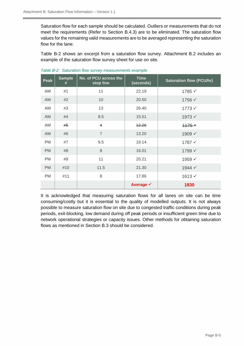
Saturation flow for each sample should be calculated. Outliers or measurements that do not

meet the requirements (Refer to Section B.4.3) are to be eliminated. The saturation flow

values for the remaining valid measurements are to be averaged representing the saturation

flow for the lane.

Table B-2 shows an excerpt from a saturation flow survey. Attachment B.2 includes an

example of the saturation flow survey sheet for use on site.

Table B-2: Saturation flow survey measurements example

Peak Sample

# No. of PCU across the

stop line Time

(seconds) Saturation flow (PCU/hr)

AM #1 11 22.19 1785

AM #2 10 20.50 1756

AM #3 13 26.40 1773

AM #4 8.5 15.51 1973

AM #5 4 12.26 1175

AM #6 7 13.20 1909

PM #7 9.5 19.14 1787

PM #8 8 16.01 1799

PM #9 11 20.21 1959

PM #10 11.5 21.30 1944

PM #11 8 17.86 1613

Average 1830

It is acknowledged that measuring saturation flows for all lanes on site can be time

consuming/costly but it is essential to the quality of modelled outputs. It is not always

possible to measure saturation flow on site due to congested traffic conditions during peak

periods, exit-blocking, low demand during off peak periods or insufficient green time due to

network operational strategies or capacity issues. Other methods for obtaining saturation

flows as mentioned in Section B.3 should be considered.


Page B-6

Measurement Requirements

The requirements for undertaking a saturation flow survey are detailed in Table B-3. It is

noted that for practical reasons it may not always be possible to meet all the requirements

when undertaking the measurements on site. Any deviations from the requirements must

be discussed in the survey report.

Table B-3: Measurement requirements of a saturation flow survey

Measurement Requirements Reasons

Measure the saturation flows for each individual lane, not a group of lanes

The traffic behaviour, discharge rate, queuing for each lane is different.

Minimum of 5 vehicles is recorded in each sample. (i.e. a minimum of 9 vehicles in the queue)

To ensure a steady queue discharge is measured.

Take measurements throughout each of the study periods

To ensure that the average saturation flow represents the site conditions for the period being modelled as saturation flow can change due to peak specific site conditions.

Minimum of 6, ideally 10, consistent samples are to be collected for each lane, across all periods

To ensure the average saturation flow is representative. To also ensure errors can be eliminated.

More samples may be required if the results are found to be significantly inconsistent to eliminate outliers.

Measure the critical approaches as the priority

To ensure that the lanes carrying most traffic are measured and modelled accurately.

Do not undertake measurements when there is exit blocking

Saturation flow rates can only occur during free flow conditions.

Record the time to the nearest 100th or 10th second where possible.

However due to the equipment availability, it is acceptable to record the time to the nearest full second.

When rounding the time to the nearest second, the resultant saturation flow value can change significantly.1

This issue is likely to be eliminated when more vehicles and longer discharge time is recorded in the sample.

Measure the time as the rear of each vehicle passes the stop line, not the front of the vehicle.

However it is noted that due to the camera positions, it is not always possible to observe the rear of the vehicles, measuring based on the front of the vehicles may be acceptable.

If measuring based on the front of the vehicle, the gap between last two vehicles in the sample is larger and this may underestimate the saturation flow.

Regardless of the chosen vehicle reference point, the measurement should be consistent.

Do not measure the time based on the centre of the vehicle.

While it counts as two vehicles passing the stop line, the discharge time does not include the front half of the first vehicle and the back half of the last vehicle. It overestimates the saturation flow value.

1 e.g. when the traffic count is 7 PCU and one surveyor measured the time of 14.49 seconds (Sat flow: 1739 PCU/hr), and another surveyor measured 14.51 seconds (Sat flow: 1736 PCU/hr). If the surveyors rounded the time to the nearest second, 14 seconds and 15 seconds, then the saturation flows are 1800 PCU/hr and 1680 PCU/hr respectively, which are significantly different.


Page B-7

B.5 Measurement of Similar Intersection

Should it not be possible to measure saturation flow at an intersection during any time

period then an alternative is to take measurements from a similar intersection. This may be

a neighbouring intersection with similar geometry, signal timings and traffic volumes. The

use of this method must be detailed in the modelling report.

B.6 Calculated from RR67

Where measurement of saturation flow is not possible for base cases or for proposed

intersections, saturation flows can be estimated based on the site geometry and lane usage.

The calculations are based on the TRL RR67 formula. For a single unopposed lane, the

formula is:

Saturation flow = 2080 - 42δGG - 100(3.25-wl) - 140δn

1+ (1.5fr

)

The formula requires the following inputs:

(δG) Gradient indicator – 1 for uphill gradient; 0 for flat or downhill.

(G) Gradient – calculated from long sections for proposed works or measured using

Google Earth or other suitable sources. This is expressed as the percentage, e.g. 1

indicates the uphill gradient is 1%. This value is required for uphill gradient only.

(wl) Lane width – measured on-site or scaled from LM plan or appropriate aerial

photographs or design drawing. The unit is metres.

(δn) Nearside indicator – 1 for nearside lane; 0 for non-nearside lane. Modellers must

refer to Section B.6.2 for guidance.

(f)Turning proportions – for a lane with mixed movements, estimate the proportion

of vehicles making each movement for the lane, expressed as a decimal figure, e.g.

0.65 indicates 65% of the traffic using the lane is turning.

(r) Radius – measured from LM plan or appropriate aerial photographs or design

drawing based on the centre of the turning vehicle movement. The unit is metres.

This value is not required for through movement.

The modeller must supply evidence of the geometric measurement (such as marked-up

plans indicating measurements) in the modelling report.

Modellers must consider if the RR67 saturation flow values are representative of the driving

behaviour at the modelled intersection, by comparing the calculated saturation flow with

available site measured values. If the average of the site values are found to be more than

5% different from the RR67 values, the modeller must apply a local site factor to the RR67

calculated lanes (Refer to Section B.7).


Page B-8

RR67 Measurement Example

Table B-4 shows the application of the RR67 formula for the southbound right turn offside

lane shown in Figure B-2.

Table B-4: Application of the RR67 formula

δG G wl δn f r Saturation

Flow (PCU/hr)

Southbound offside lane

0 flat

0 flat

4.2 0 Non

nearside

1.0 All traffic turning

22 2036

Figure B-2: Example of geometry measurement for RR67

RR67 Nearside and Offside Lanes

When using RR67 estimates for lane saturation flow, a lane needs to be identified as

nearside or offside. The interpretation of the nearside/offside setting in RR67 is vague. A

nearside lane is loosely defined as the first lane from the kerb in which a particular traffic

movement appears. Figure B-3 shows some examples of lane compositions to aid in

identification of nearside lanes.

Figure B-3: Nearside lane identification

If the selection of nearside or offside leads to significantly different engineering

consequences in the modelling, then measured or locally-derived saturation flow values

should be used to improve the accuracy of the modelling.

N/S N/S N/S N/S N/S

O/S N/S N/S N/S N/S

N/S N/S N/S N/S N/S

O/S N/S N/S N/S N/S

N/S N/S O/S N/S O/S

N/S N/S N/S N/S N/S

O/S N/S O/S O/S N/S

O/S N/S N/S N/S N/S

N/S O/S O/S O/S O/S

Note: N/S means Nearside lane and O/S means Offside lane.


Page B-9

B.7 Calculated from RR67 with a Local Factor

The saturation flow values measured on-site must be compared with the RR67-calculated

value (Refer to Section B.6). If the average of the site values are found to be more than 5%

different from the RR67 values, the modeller must apply a local site factor to the RR67

calculated lanes. For consistency, the same factor should also be applied in the option

models. Failure to apply a site factor may result in inaccurate assessment of the option

model outputs.

If modelling in LinSig, it has a built-in geometrically-calculated lane saturation flow function

based on the RR67 formula. If a local factor is required, the modeller would need to calculate

the RR67 and the factored saturation flow in a separate spreadsheet. The RR67 research

paper can be obtained from the TRL website, and the formula for a single unopposed lane

is discussed in Section B.6.1.

In the example shown in Table B-5, the site measured saturation flow is found to be on

average 93% of the RR67 equivalent values, therefore the local factor of 93% must be

applied for the remaining traffic lanes with saturation flow estimated using RR67.

Table B-5: Saturation flow site measurement and RR67 comparison

Lane

Site measured saturation

flow

RR67 calculated saturation

flow

Site measured : RR67 ratio

(local factor)

Saturation flow used

in modelling

Method

1/1 - 1809 - 1682 Factored RR67

1/2 - 1925 - 1789 Factored RR67

1/3 1889 2065 91.5% 1889 Site measurement



3/1 - 1865 - 1734 Factored RR67

3/2 - 2036 - 1893 Factored RR67

Average 93.0%

B.8 Estimated from SCATS MF Data

LX files can be used to assess maximum flow (MF) to assist in calculating saturation flow.

It is important to note that this should be used as an indication only, as MF is only reflective

of the saturation flow if the intersection was fully saturated in the preceding 24 hours. As

full saturation is not always guaranteed, Main Roads does not recommend relying on MF

for saturation flow calculations. Should the MF data be used for modelling, modellers are

required to compare the MF values with any available site measured values to determine if

the MF values are suitable for analysis.


Page B-10

References

Title Author Year

Fundamental Relationships for Traffic Flows at Signalised Intersections

Akçelik A, Besley M and Roper R, ARRB Research Report ARR340, Melbourne, Australia

1999

Guide to Traffic Management – Part 3: Traffic Studies and Analysis

Austroads Ltd, Sydney. Australia. 2013

The Prediction of Saturation Flows for Single Road Junctions Controlled (TRL RR67)

Kimber, RM, McDonald, M & Hounsell, NB., United Kingdom

1986


Page B-11

Attachment B.1 Saturation Flow Measurement Diagrams

1. At the start of green, for the lane to be measured, note the length of the queue

The first four vehicles are not included in the measurement as these will depart at sub

saturation flow rates due to reaction times and acceleration.


Page B-12

2. Start timing when the rear of the fourth vehicle passes the stop line.

3. Start the vehicle count from the fifth vehicle as it passes the stop line.


Page B-13

Note that more vehicles may join the back of the queue.

4. Stop the count when the rear of the last vehicle in the queue passes the stop line.

5. Record the time and number of vehicles discharging during the saturated period.

6. Repeat for further samples of the same lane.


Page B-14

Attachment B.2 Saturation Flow Survey Sheet

This is an example of a Saturation Flow survey sheet. Surveyors are free to set up own

survey sheets.

Appendix B: Saturation Flow Information

Documents

Transcript of Appendix B: Saturation Flow Information