Appendix A: The Fourier Transform978-3-319-30463-2/1.pdf · A.1 Properties of the Fourier Transform...

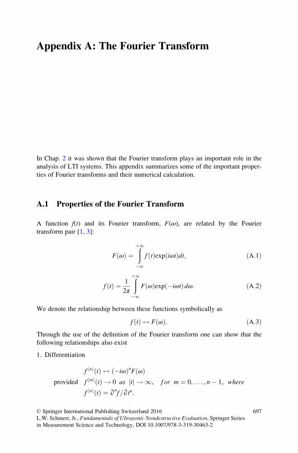
Appendix A: The Fourier Transform

In Chap. 2 it was shown that the Fourier transform plays an important role in the

analysis of LTI systems. This appendix summarizes some of the important proper-

ties of Fourier transforms and their numerical calculation.

A.1 Properties of the Fourier Transform

A function f(t) and its Fourier transform, F(ω), are related by the Fourier

transform pair [1, 3]:

F ωð Þ ¼ðþ1

�1f tð Þexp iωtð Þdt; ðA:1Þ

f tð Þ ¼ 1

2π

ðþ1

�1F ωð Þexp �iωtð Þdω: ðA:2Þ

We denote the relationship between these functions symbolically as

f tð Þ $ F ωð Þ: ðA:3ÞThrough the use of the definition of the Fourier transform one can show that the

following relationships also exist

1. Differentiation

f nð Þ tð Þ $ �iωð ÞnF ωð Þprovided f mð Þ tð Þ ! 0 as tj j ! 1, f or m ¼ 0, . . . , n� 1, where

f nð Þ tð Þ ¼ ∂nf=∂tn:

© Springer International Publishing Switzerland 2016

L.W. Schmerr, Jr., Fundamentals of Ultrasonic Nondestructive Evaluation, Springer Seriesin Measurement Science and Technology, DOI 10.1007/978-3-319-30463-2

697

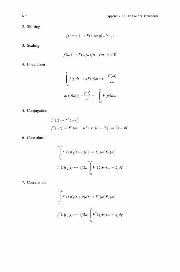
http://dx.doi.org/10.1007/978-3-319-30463-2_2

2. Shifting

f t� t0ð Þ $ F ωð Þexp �iωt0ð Þ

3. Scaling

f atð Þ $ F ω=að Þ=a f or a > 0

4. Integration

ðt�1

f tð Þdt $ πF 0ð Þδ ωð Þ � F ωð Þiω

πf 0ð Þδ tð Þ þ f tð Þit

$ðω

�1F ωð Þdω

5. Conjugation

f * tð Þ $ F* �ωð Þf * �tð Þ $ F* ωð Þ where aþ ibð Þ* ¼ a� ibð Þ

6. Convolution

ðþ1

�1f 1 τð Þf 2 t� τð Þdτ $ F1 ωð ÞF2 ωð Þ

f 1 tð Þf 2 tð Þ $ 1=2π

ðþ1

�1F1 ξð ÞF2 ω� ξð Þdξ

7. Correlation

ðþ1

�1f *1 τð Þf 2 tþ τð Þdτ $ F*

1 ωð ÞF2 ωð Þ

f *1 tð Þf 2 tð Þ $ 1=2π

ðþ1

�1F*1 ςð ÞF2 ωþ ςð Þdς

698 Appendix A: The Fourier Transform

8. Parsevals’ theorem

ðþ1

�1f *1 τð Þf 2 τð Þdτ ¼ 1=2π

ðþ1

�1F*1 ωð ÞF2 ωð Þdω

and when f 1 ¼ f 2 ¼ f

ðþ1

�1f tð Þj j2dt ¼ 1=2π

ðþ1

�1F ωð Þj j2dω

A.2 Some Fourier Transform Pairs

f tð Þ F ωð Þ

1. Dirac delta function

δ tð Þ 1

2. Heaviside step function

H tð Þ ¼1 t > 0

1=2 t ¼ 0

0 t < 0

8>><>>: πδ ωð Þ þ i

ω

3. Sign function

sgn tð Þ ¼1 t > 0

�1 t < 0

(2i

ω

4. tj j � 2

ω2

5.1

tiπ sgn ωð Þ

6. exp �atð ÞH tð Þ aþ iω

a2 þ ω2

7. Laplace function

exp �a tj jð Þ 2a

a2 þ ω2

Appendix A: The Fourier Transform 699

8. Gauss function

exp �at2� � ffiffiffi

πpa

exp �ω2=4a� �

9. Rectangular function

Π tð Þ ¼1 tj j < 1=2

0 tj j > 1=2

(sin ω=2ð Þω=2

¼ sinc ω=2πð Þ

10.sin atð Þπt

Π ω=2að Þ

11. Triangular function

Λ tð Þ ¼1� tj j tj j � 1

0 tj j > 1

(sinc2 ω=2πð Þ

A.3 The Discrete Fourier Transform

The typical output of an ultrasonic system is an analog voltage versus time wave

form. Most modern NDEmeasurement systems digitize such wave forms so that the

sampled values can be manipulated by computer. In this section we will examine

the consequences of dealing with a sampled signal and consider the way in which

the Fourier transform can be computed from these samples in an efficient manner.

To begin, we rewrite the Fourier transform (and its inverse) in terms of the

frequency f (in Hertz) instead of the circular frequency ω:

X fð Þ ¼ðþ1

�1x tð Þexp 2πi f tð Þdt

x tð Þ ¼ðþ1

�1X fð Þexp �2πi f tð Þdf :

ðA:4Þ

Now we consider the discrete (sampled) values of x(t) at the times tj ¼ jΔt wherej ¼ 0, � 1, � 2, . . . and we let f s ¼ 1=Δt. Then these sampled values are given by

x tj� � ¼ ðþ1

�1X fð Þexp �2πi j f=f sð Þdf ; ðA:5Þ


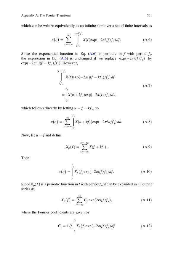
which can be written equivalently as an infinite sum over a set of finite intervals as

x tj� � ¼ X1

k¼�1

ðkþ1ð Þf s

k f s

X fð Þexp �2πi j f=f sð Þdf : ðA:6Þ

Since the exponential function in Eq. (A.6) is periodic in f with period fs,the expression in Eq. (A.6) is unchanged if we replace exp �2πi j f=f sð Þ by

exp �2πi j f � kf sð Þ=f sð Þ. However,

ðkþ1ð Þf s

kf s

X fð Þexp �2πi j f � kf sð Þ=f sð Þdf

¼ðf s0

X uþ kf sð Þexp �2πi j u=f sð Þdu;

ðA:7Þ

which follows directly by letting u ¼ f � k f s, so

x tj� � ¼ X1

k¼�1

ðf s0

X uþ kf sð Þexp �2πi u=f sð Þdu: ðA:8Þ

Now, let u ¼ f and define

Xp fð Þ ¼Xk¼þ1

k¼�1X f þ kf sð Þ: ðA:9Þ

Then

x tj� � ¼ ðf s

0

Xp fð Þexp �2πij f=f sð Þdf : ðA:10Þ

Since Xp( f ) is a periodic function in f with period fs, it can be expanded in a Fourierseries as

Xp fð Þ ¼X1j¼�1

Cj exp 2πij f=f sð Þ; ðA:11Þ

where the Fourier coefficients are given by

Cj ¼ 1=f s

ðf s0

Xp fð Þexp �2πij f=f sð Þdf ðA:12Þ


Recognizing these Fourier coefficients as just x(tj)/fs from Eq. (A.11), we have

Xp fð Þ ¼ 1=f sX1j¼�1

x tj� �

exp 2πij f=f sð Þ: ðA:13Þ

Thus, knowing all the sampled values of x(t), Eq. (A.13) shows that we recover

Xp( f ) rather than X( f ) itself. The function Xp( f ) differs from our original X( f ) bythe sum of X( f )’s displaced at multiples of fs (Fig. A.1). This difference is referredto as aliasing. If X( f ) is band limited, i.e. X( f ) ¼ 0 for fj j > fmax where fmax is the

maximum frequency in the signal, then we see that Xp fð Þ ¼ X fð Þ for fj j < f max iff s � 2 fmax (Fig. A.2). Even when X( f ) is not band limited, if fmax represents the

– fs

Xp ( f )

X ( f )

fsf

f

a

b

Fig. A.1 (a) A Fourier

transform spectra, X( f ),and (b) its infinitelyrepeated periodic

replica, Xp( f )

– fs – fmax fmax

– fmax fmax

Xp ( f )

X ( f )

fsf

f

a

b

Fig. A.2 (a) A Fourier

transform spectra, X( f ), ofa band limited function and

(b) its infinitely repeated

replica, Xp( f ), if f s > 2f max


maximum significant frequency contained in the signal we will have Xp fð Þ ¼ X fð Þapproximately for fj j < f max, again as long as

f s � 2fmax; ðA:14Þwhich is the well-known Nyquist sampling criterion. This criterion says that in

order to recover a true replica of the frequency spectra of our original signal in the

frequency range fj j < f max, we should sample our signal at least twice the value of

the maximum significant frequency in that signal. Since the Nyquist criterion only

gives a lower bound for the sampling frequency, in practice we usually sample a

signal at a much higher rate such as 5fmax ! 10f max to be conservative.

Now, suppose that we sample Xp( f ) in Eq. (A.13) at f ¼ nΔf , n ¼ 0, � 1,

�2, . . . where Δf ¼ 1=T and T is the total time interval sampled. Then

Xp f nð Þ ¼ 1=f sX1j¼�1

x tj� �

exp 2πi jn=Tf sð Þ: ðA:15Þ

However, if we take Tf s ¼ N where N is an integer and use the fact that exp(2πijn/N ) is periodic in j with period N, we can rewrite Xp( fn) as

Xp f nð Þ ¼ T=NXN�1

j¼0

xp tj� �

exp 2πijn=Nð Þ; ðA:16Þ

where

xp tj� � ¼ X1

k¼�1x tj þ kT� � ðA:17Þ

are the sampled values of a periodic function xp(t) given by

xp tð Þ ¼X1k¼�1

x tþ kTð Þ; ðA:18Þ

which is formed from x(t) in the same manner as Xp( f ) is formed from X( f ).Eq. (A.16) is in the form of an inverse discrete Fourier transform [2] that relates the

sampled values of Xp( f ) to the sampled values of xp(t). If aliasing is negligible, thenEq. (A.16) is also a relation between the sampled values of our original wave form

x(t) and its frequency components X( f ).Given the sampled values Xp( f ), we can also recover xp(t) via an inverse

relationship similar to Eq. (A.16). To see this consider the sum

XN�1

n¼0

Xp f nð Þexp �2πi kn=Nð Þ ¼ T=NXN�1

n¼0

XN�1

j¼0

xp tj� �

exp �2πi k � jð Þn=Nð Þ: ðA:19Þ


However,

1=NXN�1

n¼0

exp �2πi k � jð Þn=Nð Þ ¼ Δ j� kð Þ; ðA:20Þ

where Δ j� kð Þ is the discrete delta function, having a sampling property similar to

the Dirac delta function (see problem A.1), i.e.

XN�1

j¼0

cjΔ j� kð Þ ¼ ck k ¼ 0, 1, 2, . . .N � 1 ðA:21Þ

Thus, we find

T xp tkð Þ ¼XN�1

n¼0

Xp f nð Þexp �2πi kn=Nð Þ; ðA:22Þ

which is the desired inversion formula. In the absence of aliasing, the discrete

forward Fourier transform pair (Eq. (A.22) and Eq. (A.16)) give us an explicit way

to calculate sampled values of the Fourier transform X( f ) directly from the sampled

values of the wave form x(t) and vice versa. However, for large N, this may still

involve a considerable amount of computation. Fortunately, there is a way to reduce

the computation required as discussed in the next section.

A.4 The Fast Fourier Transform

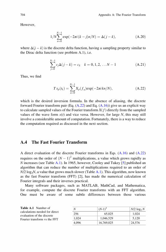
A direct evaluation of the discrete Fourier transforms in Eqs. (A.16) and (A.22)

requires on the order of N � 1ð Þ2 multiplications, a value which grows rapidly as

N increases (see Table A.1). In 1965, however, Cooley and Tukey [5] published an

algorithm that can reduce the number of multiplications required to an order of

N/2 log2N, a value that grows much slower (Table A.1). This algorithm, now known

as the fast Fourier transform (FFT) [2], has made the numerical calculation of

Fourier integrals and their inverses practical.

Many software packages, such as MATLAB, MathCad, and Mathematica,

for example, compute the discrete Fourier transforms with an FFT algorithm.

One must be aware of some subtle differences between those various

Table A.1 Number of

calculations needed for direct

evaluation of the discrete

Fourier transform vs the FFT

N (N-1)2 N/2 log2 N

256 65,025 1,024

1,024 1,046,529 5,120

4,096 16,769,025 24,576


implementations. In this book we have defined the forward and inverse Fourier

transforms by the relations in Eqs. (A.1) and (A.2). However, we can also define

these pair of equations in the forms

~F ωð Þ ¼ n1

ðþ1

�1f tð Þexp �iωtð Þ

f tð Þ ¼ n2

ðþ1

�1

~F ωð Þexp �iωtð ÞðA:23Þ

as long as the constants (n1, n2) satisfy n1n2 ¼ 1=2π. Different choices will obvi-ously lead to different values for the Fourier transform which is why we have placed

a tilde over the transform in Eq. (A.23). In analytical discussions of wave

propagation, one must be especially aware of the signs chosen in Eq. (A.23),

since this can alter the physical meaning of the result. In Chap. 4, for example,

we expressed a 1-D plane wave traveling in the + x-direction by its Fourier

transform (see Eq. (4.5)) as

f t� x=cð Þ ¼ 1

2π

ðþ1

�1F ωð Þexp iω x=c� tð Þ½ �dω; ðA:24aÞ

where

F ωð Þ ¼ðþ1

�1f tð Þexp iωtð Þdt: ðA:24bÞ

Equation (A.24a) can be interpreted as representing the traveling pulse as a super-

position of harmonic waves of the form F ωð Þexp ikx� iωtð Þ. This corresponds tochoosing the minus sign in exponential term for the inverse Fourier transform as

done in Eq. (A.2). If we had chosen the plus sign instead then we would have

instead of Eq. (A.24a) the result:

f t� x=cð Þ ¼ 1

2π

ðþ1

�1

~F ωð Þexp iω �x=cþ tð Þ½ �dω; ðA:25Þ

where the Fourier transform is now the complex conjugate of the Fourier transform

appearing in Eq. (A.24a) since

~F ωð Þ ¼ðþ1

�1f tð Þexp �iωtð Þdt ¼ F* ωð Þ: ðA:26Þ


http://dx.doi.org/10.1007/978-3-319-30463-2_4

http://dx.doi.org/10.1007/978-3-319-30463-2_4

In discussing harmonic waves some authors will implicitly assume one of these sign

choices without stating them explicitly. For example, a plane wave traveling in the

+x-direction may be written as A ωð Þexp �ikxð Þ. This means that the author is

implicitly using the form of Eq. (A.25) and the complex amplitude, A(ω), will bethe complex conjugate of the same amplitude obtained when using our definitions

of Eqs. (A.1) and (A.2). Differences due to different definitions can also arise in the

case of the discrete Fourier transform and its implementation. In our case, we

derived the discrete Fourier transform and its inverse directly from Eqs. (A.1) and

(A.2), obtaining Eqs. (A.16) and (A.22), which we rewrite here as:

Xp f nð Þ ¼ ΔtXN�1

j¼0

x tj� �

exp 2πi jn=Nð Þ

xp tkð Þ ¼ 1

NΔt

XN�1

n¼0

Xp f nð Þexp �2πi kn=Nð Þ:ðA:27Þ

Other equivalent forms are

~Xp f nð Þ ¼ m1

XN�1

j¼0

x tj� �

exp �2πi jn=Nð Þ

xp tkð Þ ¼ m2

XN�1

n¼0

~Xp f nð Þexp �2πi kn=Nð ÞðA:28Þ

as long as the constants (m1,m2) satisfy m1m2 ¼ 1=N. In this book, we will

exclusively use Eqs. (A.1) and (A.2) for the Fourier transform pair and

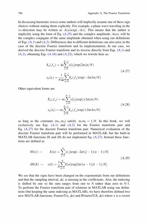
Eq. (A.27) for the discrete Fourier transform pair. Numerical evaluation of the

discrete Fourier transform pair will be performed in MATLAB, but the built-in

MATLAB functions fft and ifft do not implement Eq. (A.27). Instead these func-

tions are defined as

fft xð Þ ! X nð Þ ¼XNj¼1

x jð Þexp �2πi j� 1ð Þ n� 1ð Þ=N½ �

ifft Xð Þ ! x kð Þ ¼ 1

N

XNn¼1

X nð Þexp 2πi n� 1ð Þ k � 1ð Þ=N½ �:ðA:29Þ

We see that the signs have been changed on the exponentials from our definitions

and that the sampling interval, Δt, is missing in the coefficients. Also, the indexing

is shifted by one so the sum ranges from one to N rather than zero to N-1.To perform the Fourier transform pair of relations in MATLAB using our defini-

tions (but keeping the same indexing as MATLAB), we have therefore defined two

new MATLAB functions, FourierT(x,Δt) and IFourierT(X,Δt) where x is a vector


or matrix of N sampled time domain values and X is a vector or matrix of N sampled

frequency domain values. As with the built-in MATLAB functions, if the inputs are

matrices, then the sampled data is assumed to be arranged in columns and the

Fourier transforms or their inverse are performed on those columns. More details on

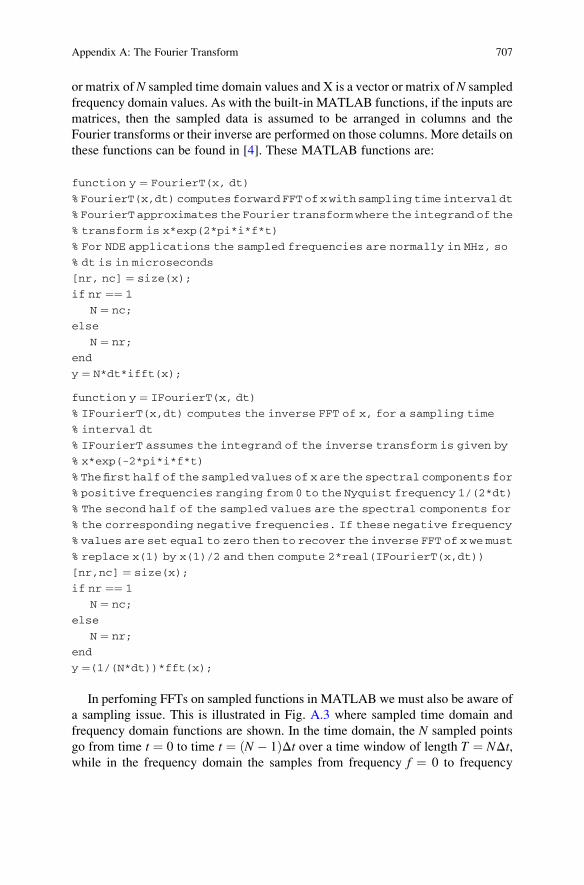
these functions can be found in [4]. These MATLAB functions are:

function y ¼ FourierT(x, dt)

%FourierT(x,dt)computesforwardFFTofxwithsamplingtimeintervaldt

% FourierT approximates the Fourier transform where the integrand of the

% transform is x*exp(2*pi*i*f*t)

% For NDE applications the sampled frequencies are normally in MHz, so

% dt is in microseconds

[nr, nc] ¼ size(x);

if nr ¼¼ 1

N ¼ nc;

else

N ¼ nr;

end

y ¼ N*dt*ifft(x);

function y ¼ IFourierT(x, dt)

% IFourierT(x,dt) computes the inverse FFT of x, for a sampling time

% interval dt

% IFourierT assumes the integrand of the inverse transform is given by

% x*exp(-2*pi*i*f*t)

% The first half of the sampled values of x are the spectral components for

% positive frequencies ranging from 0 to the Nyquist frequency 1/(2*dt)

% The second half of the sampled values are the spectral components for

% the corresponding negative frequencies. If these negative frequency

% values are set equal to zero then to recover the inverse FFT of x we must

% replace x(1) by x(1)/2 and then compute 2*real(IFourierT(x,dt))

[nr,nc] ¼ size(x);

if nr ¼¼ 1

N ¼ nc;

else

N ¼ nr;

end

y ¼(1/(N*dt))*fft(x);

In perfoming FFTs on sampled functions in MATLAB we must also be aware of

a sampling issue. This is illustrated in Fig. A.3 where sampled time domain and

frequency domain functions are shown. In the time domain, the N sampled points

go from time t ¼ 0 to time t ¼ N � 1ð ÞΔt over a time window of length T ¼ NΔt,while in the frequency domain the samples from frequency f ¼ 0 to frequency


f ¼ N � 1ð Þ=Δt over a frequency window of length f s ¼ 1=Δt. If we use the

MATLAB function e ¼ linspace(0, E, N) to generate N sampled values e

(representing times or frequencies) over the interval from zero to E we will not

obtain the proper sampled values shown in Fig. A.3 and this application of linspace

will produce an incorrect sampling interval given by Δe ¼ E= N � 1ð Þ. Thus, weneed to have a function that does produce the proper sampled values. The function

s_space listed below is a small modification of linspace that fills that need and

should be used in place of linspace when generating sampled time or frequency

values for performing Fourier analysis with FFTs:

function y ¼ s_space(xstart, xend, num)

% s_space(xstart,xend, num) generates num evenly spaced sampled

% values from xstart to (xend - dx), where dx ¼ (xend – xstart)/num is

% the sample spacing. This is useful in FFT analysis where we generate

% sampled periodic functions. Example: generate 1000

% sampled frequencies from 0 to 100MHz via f ¼s_space(0,100,1000);

% In this case the last value of f will be 99.9 MHz and the

% sampling interval will be 100/1000 ¼0.1 MHz.

ye ¼ linspace(xstart, xend, num+1);

y ¼ ye(1:num);

Using s_space in conjunction with FourierT and IFourierT gives you the tools

necessary to perform time and frequency domain evaluations consistent with the

Fourier transform pair definitions used throughout this book. For additional infor-

mation on Fourier analysis see [4].

Fig. A.3 A sampled

periodic time domain

function and its Fourier

transform, showing the

N sampled values one

obtains with an FFT


A.5 Problems

A.1. Define the discrete delta function, Δ, as

Δ k � nð Þ ¼1 k ¼ n

0 k 6¼ n

(:

From this definition, the sampling property of the discrete delta function

(Eq. (A.21)) follows directly. Show that

Δ k � nð Þ ¼ 1=NXN�1

m¼0

exp 2πim k � nð Þ=Nð Þ

i.e. prove that Eq. (A.20) is valid. (Hint: show that the series can be summed

explicitly to the value

wN k�nð Þ � 1� �

= w k�nð Þ � 1� �

;

where w ¼ exp 2πi=Nð Þ.A.2. Consider the wave form given by

x tð Þ ¼e�t t > 0

0 t < 0

(;

where t is measured in μ sec.

(a) What is the analytical Fourier transform, X( f ), of this function? Plot

the real and imaginary parts of X( f ) from f ¼ 0 to f ¼ 4 MHz. Also

plot the magnitude of X( f ) over this same range.

(b) Suppose we sample x(t) from t ¼ 0 to t ¼ 8 μ sec with N ¼ 16, i.e.

Δt ¼ 0:5μ sec . Note that there is a discontinuity in x(t) at t¼ 0. Take the

value to be 0.5 at this sample point. Why do we do this? Plot the sampled

function and compare with the original function. Is the sampling ade-

quate to represent this function?

(c) Compute the FFT of this sampled wave form. What is fs here? Plot the

sampled values of the frequency components from f ¼ 0 to f ¼ 2 MHz.

Compare with your results from part (a). Is aliasing a problem here?

(d) Repeat parts (b) and (c) changing only N to N ¼ 32. How do your results

change in parts (b) and (c)?

(e) Repeat parts (b) and (c), changing T to T ¼ 16 μ sec and N to N ¼ 32.

How do your results change from parts (b) and (c)?


References

1. A. Papoulis, Signal Analysis (McGraw-Hill, New York, 1977)

2. C.S. Burrus, T.W. Parks, DFT, FFT and Convolution Algorithms (Wiley, New York, 1985)

3. J.S. Walker, Fast Fourier Transforms, 2nd edn. (CRC, New York, 1996)

4. L.W. Schmerr, S-J. Song, Ultrasonic Nondestructive Evaluation Systems: Models and Mea-surements (Springer, New York, 2007)

5. J.W. Cooley, J.W. Tukey, An algorithm for the machine calculation of complex Fourier series,

Math. Comput., 19, 297–301, (1965)


Appendix B: The Dirac Delta Function

In Chap. 2 we saw that the delta function also plays an important role in determin-

ing the response of LTI systems since it acts as an ideal input function whose

Fourier transform contains all frequencies equally weighted. Strictly speaking the

delta function is not an ordinary function but is a distribution [1, 2]. However, we

will continue to speak of δ(t) as an ordinary function, remembering that δ only has ameaning in terms of its sifting property, i.e.

ðba

δ t� xð Þf xð Þdx ¼ f tð Þ a < t < b

¼ 0 t < a or t > b

¼ f tð Þ=2 t ¼ a or t ¼ b:

ðB:1Þ

The delta function also plays an important role in dealing with integral equations

and boundary value problems, as discussed in Chap. 5 [3].

B.1 Properties of the Delta Function

Several of the more useful properties of the delta function are summarized below,

given the real constants a, b, c, and A and the function f(t):

1. Scaling properties

δt� c

b

� �¼ bj jδ t� cð Þ

δ �tð Þ ¼ δ tð Þ

δ f tð Þ½ � ¼Xk

δ t� tkð Þf 0 tkð Þj j f tkð Þ ¼ 0, f

0 ¼ df=dt



711

http://dx.doi.org/10.1007/978-3-319-30463-2_2

http://dx.doi.org/10.1007/978-3-319-30463-2_5

2. Properties in product form

f tð Þδ t� cð Þ ¼ f cð Þδ t� cð Þδ tð Þδ t� cð Þ ¼ 0 c 6¼ 0

δ t� cð Þδ t� cð Þ is not defined

3. Integrals

ðþ1

�1Aδ t� cð Þdt ¼ A

ðþ1

�1δ t� cð Þ ¼ 1

ðt�1

δ u� cð Þdu ¼ H t� cð Þ where H tð Þ is the unit step function:

H tð Þ ¼1 t > 0

1=2 t ¼ o

0 t < 0

8>><>>:

4. Derivatives

ðba

f tð Þδ nð Þ t� cð Þ dt ¼ �1ð Þnf nð Þ cð Þ a < c < b, f nð Þ ¼ dnf=dtn

5. Fourier Transform pair

1 ¼ðþ1

�1δ tð Þexp iωtð Þdt

δ tð Þ ¼ 1

2π

ðþ1

�1exp �iωtð Þdω

712 Appendix B: The Dirac Delta Function

References

1. M.J. Lighthill, Introduction to Fourier Analysis and Generalized Functions (Cambridge

University Press, 1958)

2. L. Schwartz, Mathematics for the Physical Sciences (Addison Wesley, Reading, 1966)

3. I. Stakgold, Boundary Value Problems of Mathematical Physics, Vols. I, II (Macmillan,

New York, 1968)

Appendix B: The Dirac Delta Function 713

Appendix C: Basic Notations and Concepts

This Appendix will give a brief discussion of indicial and vector notation and

review some of the basic concepts of motion, mass, and stress/strain needed for our

consideration of the equations governing elastic media. Continuum mechanics texts

[1–6] are good sources for a more complete description of these topics.

C.1 Indicial Notation

The equations involved in elasticity problems are often algebraically quite com-

plex. The use of Cartesian tensor (index) notation significantly simplifies the

expression and manipulation of such equations.

In index notation, the Cartesian coordinates (x, y, z) will be denoted by the

subscripted variables (x1, x2, x3) (Fig. C.1) and the corresponding unit base vectors

by the vectors (e1, e2, e3). An arbitrary three-dimensional vector u with Cartesian

components (u1, u2, u3) can thus be written as

u ¼X3i¼1

ui ei: ðC:1Þ

If we adopt the Einstein summation convention, where the appearance twice of the

same index symbol implies summation over the range of that index, Eq. (C.1) can

be written simply as

u ¼ ui ei: ðC:2Þ

In Eq. (C.2), the repeated index i is merely a “dummy” index since it is “summed

out”. We can replace any such dummy index symbol by any other symbol without



715

changing the meaning of the equation. Thus, for example, the following expressions

are all equally valid:

f ¼ apbp ¼ aqbq ðC:3aÞ

u ¼ uiei ¼ ukek ðC:3bÞ

wi ¼ aijxj ¼ aikxk i ¼ 1, 2, 3ð Þ ðC:3cÞ

σij ¼ Cijklekl ¼ Cijlmelm: ðC:3dÞ

In Eq. (C.3c), the j and k indices are dummy indices that assume all values in the

range (1, 2, 3) while the i index is a “free” index which assumes only any one of

these values at a time. In some cases, as in Eq. (C.3c), we will show the range of the

free indices explicitly. Otherwise, the range will be assumed to be implicitly given

by (1, 2, 3). In Eq. (C.3d), for example, both free indices (i, j) can take on any one ofthe three values (1, 2, 3).

Quantities with no indices (see f in Eq. (C.3a)) are scalars, or tensors of order

zero, while quantities with only one free index are normally components of vectors,

or tensors of order one (see ap, bp,wi in Eqs. (C.3b, c)). Similarly, quantities with

n free indices are often components of tensors of order n. For example, σij, and eklare components of tensors of order two, while Cijkl is a tensor of order four. Whether

or not a quantity is a tensor of a particular order, of course, depends on its behavior

under coordinate transformation [1].

Several special quantities appear frequently in indicial notation. One of these is

the Kronecker delta tensor, δij, defined as

δij ¼1 i ¼ j

0 i 6¼ j

(: ðC:4Þ

e2

e1

e3 x (x1)

y (x2)

z (x3)

Fig. C.1 Cartesian

coordinates and base

unit vectors

716 Appendix C: Basic Notations and Concepts

Another common quantity is the alternating tensor, εijk, defined by

εijk ¼þ1 i; j; kð Þ an even permutation of 1; 2; 3ð Þ�1 i; j; kð Þ an odd permutation of 1; 2; 3ð Þ0 if any two i; j; kð Þ indices are equal

8>><>>: : ðC:5Þ

The Kronecker delta tensor and the alternating tensor are related through a useful

expression called the ε� δ identity given by

εijkεirs ¼ δjrδks � δjsδkr; ðC:6Þ

which can be verified by direct evaluation.

Also, we note that in index notation partial differentiation with respect to an

indexed variable is indicated by a comma followed by the index symbol such as, for

example,

f ,k ¼ ∂f=∂xk wi, j ¼ ∂wi=∂xj:

Since the variable name is dropped by this convention, where derivatives of more

than one variable occur in the same expression, it is sometimes convenient to

indicate which variable is being differentiated by using distinct index symbols.

To illustrate, consider the function f x; yð Þ ¼ f x1; x2; x3; y1; y2; y3ð Þ. We write

f ,k ¼ ∂f=∂xk f ,K ¼ ∂f=∂yK

so

f , iK ¼ ∂2f =∂xi∂yK

f ,KK ¼ ∂2f=∂yK∂yK

f ,kk ¼ ∂2f=∂xk∂xk

etc.

Using indicial notation, many of the standard vector operations are easily

written:

1. Dot product of two vectors, u and v

u � v ¼ uivi

2. The vector cross product

if c ¼ a b then ci ¼ εijkajbk

Appendix C: Basic Notations and Concepts 717

3. The vector operator del

∇ ¼ e1∂ð Þ=∂x1 þ e2∂ð Þ=∂x2 þ e3∂ð Þ=∂x3¼ ei∂ð Þ=∂xi ¼ eið Þ, i

4. The gradient of a scalar field, f

∇f ¼ f ,pep

5. The divergence of a vector field, f

∇ � f ¼ f i, i

6. The curl of a vector field, u

if q ¼ ∇ u then qi ¼ εijkuk, j

7. The Laplacian of a scalar field, f

∇2f ¼ ∇ � ∇fð Þ ¼ f ,kk

8. The Laplacian of a vector field, u

∇2u ¼ uk, jjek

C.2 Integral Theorems

C.2.1 Gauss’ Theorem

We will frequently make use of a fundamental integral theorem, called Gauss’theorem, which transforms a volume integral into an integral over the surface of

that volume. In its most general form, Gauss’ theorem states that for a volume

V bounded by a surface S and for a differentiable tensor field, aij . . . n, of any order

we have ðV

aij...n,k dV ¼ðS

nkaij...n dS; ðC:7Þ

where nk are components of the unit normal vector of the surface S which points

outward from V. Some important special cases of Gauss’ theorem arise from the

following specific choices for the general tensor a:


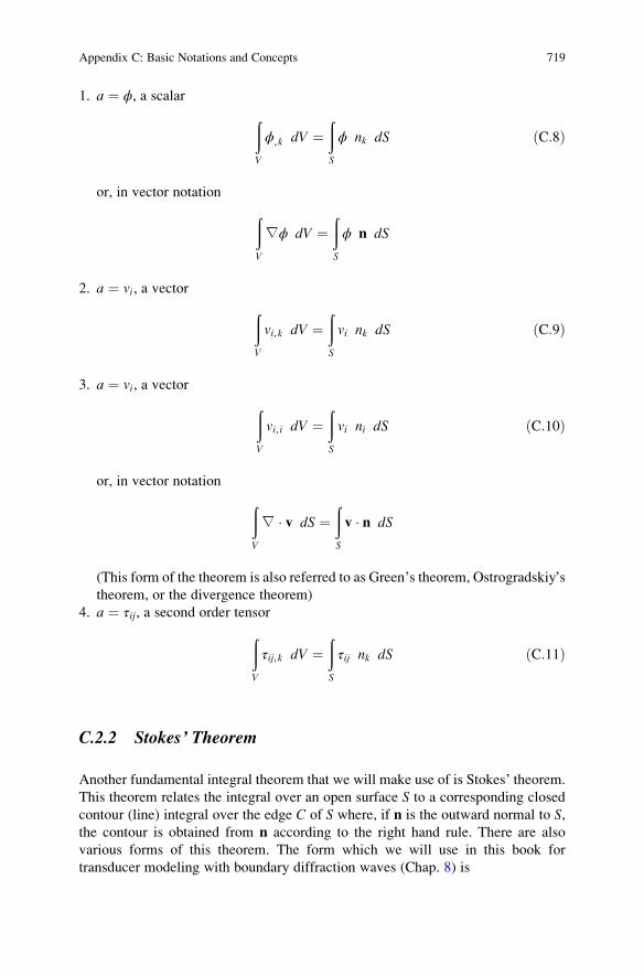
1. a ¼ ϕ, a scalar ðV

ϕ,k dV ¼ðS

ϕ nk dS ðC:8Þ

or, in vector notation ðV

∇ϕ dV ¼ðS

ϕ n dS

2. a ¼ vi, a vector ðV

vi,k dV ¼ðS

vi nk dS ðC:9Þ

3. a ¼ vi, a vector ðV

vi, i dV ¼ðS

vi ni dS ðC:10Þ

or, in vector notation ðV

∇ � v dS ¼ðS

v � n dS

(This form of the theorem is also referred to as Green’s theorem, Ostrogradskiy’stheorem, or the divergence theorem)

4. a ¼ τij, a second order tensor

ðV

τij,k dV ¼ðS

τij nk dS ðC:11Þ

C.2.2 Stokes’ Theorem

Another fundamental integral theorem that we will make use of is Stokes’ theorem.

This theorem relates the integral over an open surface S to a corresponding closed

contour (line) integral over the edge C of S where, if n is the outward normal to S,the contour is obtained from n according to the right hand rule. There are also

various forms of this theorem. The form which we will use in this book for

transducer modeling with boundary diffraction waves (Chap. 8) is


http://dx.doi.org/10.1007/978-3-319-30463-2_8

ðS

∇ fð Þ � ndS ¼IC

f � dc: ðC:12Þ

Several other forms of Stokes’ theorem that are particularly useful in regularizing

the hypersingular integral equations appearing in crack problems (see Chap. 5) are

1. For a vector fkðS

∂f k=∂xrð Þnk � ∂f k=∂xkð Þnr½ �dS ¼IC

εkrqf kdxq: ðC:13Þ

2. For a tensor fkmðS

∂f km=∂xrð Þnk � ∂f km=∂xkð Þnr½ �dS ¼IC

εkrqf kmdxq: ðC:14Þ

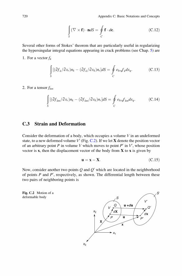
C.3 Strain and Deformation

Consider the deformation of a body, which occupies a volume V in an undeformed

state, to a new deformed volume V0 (Fig. C.2). If we letX denote the position vector

of an arbitrary point P in volume V which moves to point P0 in V0, whose positionvector is x, then the displacement vector of the body from X to x is given by

u ¼ x� X: ðC:15Þ

Now, consider another two points Q and Q0 which are located in the neighborhood

of points P and P0, respectively, as shown. The differential length between these

two pairs of neighboring points is

x3

x1

x2

S

QQ’

V’

S’

V

xX

u +duu +du

uuP P’

dXdx

Fig. C.2 Motion of a

deformable body


http://dx.doi.org/10.1007/978-3-319-30463-2_5

dS ¼ dXidXið Þ1=2 ðC:16Þ

in volume V, and

ds ¼ dxidxið Þ1=2 ðC:17Þ

in volume V0. Any distortion that occurs between these points during the deforma-

tion is given by

ds2 � dS2 ¼ dxidxi � dXidXi

¼ δij � Xk, iXk, j

� �dxidxj:

ðC:18Þ

Thus, this local distortion, or strain, is described by the second order tensor, εij,given by

εij ¼ 1

2δij � Xk, iXk, j

� �; ðC:19Þ

where the factor of 1/2 is introduced merely for convenience. The quantity εij isknown as the Almanski strain tensor. From Eq. (C.15), the Almanski strain tensor

can be rewritten in terms of the displacement components, ui, as

εij ¼ 1

2ui, j þ uj, i � uk, iuk, j� �

: ðC:20Þ

In all the applications considered in this book, the displacement gradients will be

everywhere small, so to first order we can write εij ¼ eij where

eij ¼ 1

2ui, j þ uj, i� � ðC:21Þ

is the Cauchy strain tensor. Since to first order we also have a change in displace-

ment, dui, given by

dui ¼ ui, j dxj

¼ 12ui, j þ uj, i� �

dxj þ 12ui, j � uj, i� �

dxj

¼ eijdxj þ ωijdxj;

ðC:22Þ

whereωij ¼ 12ui, j � uj, i� �

is the rotation tensor, we see that locally the kinematics of

motion can be decomposed into two parts. The first part, eij ¼ 12ui, j þ uj, i� �

is due to

the distortion (strain) occurring while the second part is due to a local rotation, ωij.

To see that ωij does indeed represent a local rotation, we note that we may write

ωij ¼ �1

2εijkωk ðC:23Þ


in terms of the components of a rotation vector, ωk, given by

ω ¼ ∇ u ðC:24Þso that the total change in displacement du can be written in vector notation, from

Eq. (C.22) as

du ¼ e � dxþ 1

2ω dx: ðC:25Þ

Since we will assume the displacement (and velocity) gradients of the motion are

everywhere small, these gradients will also be neglected when computing the

velocity, v, and the acceleration, a. For the velocity v, for example, we have

v x; tð Þ ¼ Du x; tð Þ=Dt; ðC:26Þwhere

D=Dt ¼ ∂=∂tþ v �∇ ðC:27Þis a total material time derivative. Thus for small displacement gradients we have

vi x; tð Þ ¼ ∂ui x; tð Þ=∂t: ðC:28ÞSimilarly, for the acceleration

a x; tð Þ ¼ Dv x; tð Þ=Dt ¼ ∂v x; tð Þ=∂tþ v x; tð Þ �∇½ �v x; tð Þ; ðC:29Þ

which for small velocity gradients becomes, in component form

ai x; tð Þ ¼ ∂vi x; tð Þ=∂t ¼ ∂2ui x; tð Þ=∂t2: ðC:30Þ

C.4 Conservation of Mass

If we let ρ0(X) be the mass density of the material in some original volume V at a

fixed time t ¼ 0 (Fig. C.2) and ρ(x, t) the corresponding density in volume V0 attime t, then by conservation of mass we haveð

V0

ρ x; tð Þdx1dx2dx3 ¼ðV

ρ0 Xð ÞdX1dX2dX3

or ðV0

ρ x X; tð Þ, tð ÞJ � ρ0 Xð Þ½ �dX1dX2dX3; ðC:31Þ


where J ¼ ∂ x1; x2; x3ð Þ=∂ X1;X2;X3ð Þ is a Jacobian [1] of the transformation from

V to V0. Since volume V0 is arbitrary, we must have

ρJ ¼ ρ0: ðC:32Þ

For small displacement gradients, however, it can be shown that the Jacobian is

approximately

J ¼ 1þ uk,kð Þ ðC:33Þ

so that to first order

ρ ¼ ρ0 1� uk,kð Þ ffi ρ0: ðC:34Þ

In most of our discussions we will take the original density, ρ0, to be independent ofX, so that Eq. (C.34) then shows that ρ is also, to first order, merely a constant.

C.5 Stress

C.5.1 The Traction Vector

Consider a volume V of material which is acted upon by a set of forces as shown in

Fig. C.3a. If we imagine passing a cutting plane with unit normal vector, n, through

an arbitrary point P in this body, then we can separate the body into two parts as

shown in Fig. C.3b. For part V�, on a small area ΔA at point P (on the planar cut

exposed by the cutting plane) there will be a net force ΔF acting on V� due to the

S

V

V–

ΔA

ΔA

ΔF − ΔF− nn

P

V+

F1

F1

F2

F3

F2

F3

a bFig. C.3 a A body acted

upon by external forces, and

b the internal (distributed)

forces acting from one part

of the body on the

adjacent part


internal forces exerted across the plane by Vþ. We define the traction vector, t(n),

acting at P as

t nð Þ ¼ limΔA!0

ΔF=ΔA: ðC:35Þ

Note that since an equal and opposite force, �ΔF, acts on an identical area ΔA for

Vþ with unit normal -n, it follows that

t �nð Þ ¼ �t nð Þ; ðC:36Þwhich is just a statement of Newton’s third law.

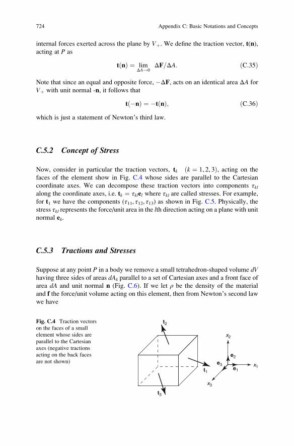
C.5.2 Concept of Stress

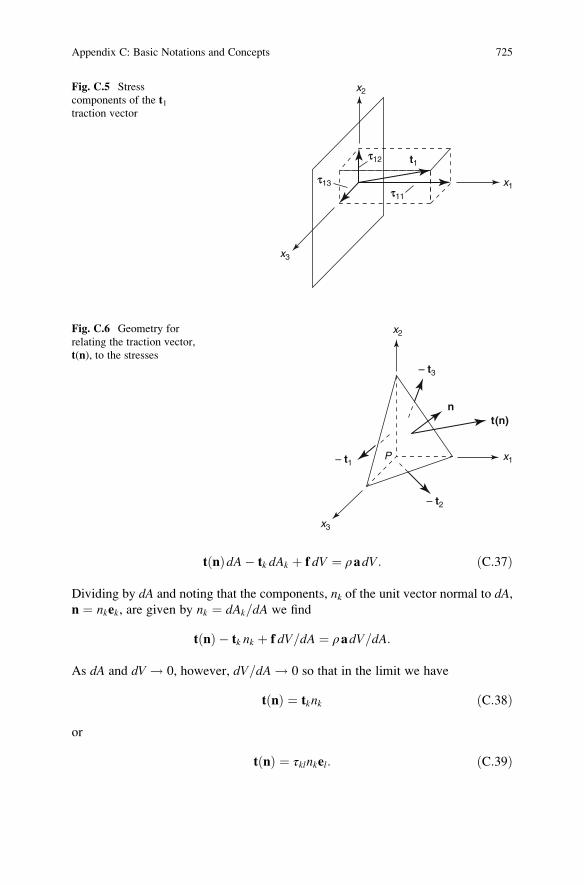
Now, consider in particular the traction vectors, tk k ¼ 1, 2, 3ð Þ, acting on the

faces of the element show in Fig. C.4 whose sides are parallel to the Cartesian

coordinate axes. We can decompose these traction vectors into components τklalong the coordinate axes, i.e. tk ¼ τklel where τkl are called stresses. For example,

for t1 we have the components (τ11, τ12, τ13) as shown in Fig. C.5. Physically, the

stress τkl represents the force/unit area in the lth direction acting on a plane with unitnormal ek.

C.5.3 Tractions and Stresses

Suppose at any point P in a body we remove a small tetrahedron-shaped volume dVhaving three sides of areas dAk parallel to a set of Cartesian axes and a front face of

area dA and unit normal n (Fig. C.6). If we let ρ be the density of the material

and f the force/unit volume acting on this element, then from Newton’s second lawwe have

t3

t1e3

e2

e1

x3

x1

x2

t2Fig. C.4 Traction vectors

on the faces of a small

element whose sides are

parallel to the Cartesian

axes (negative tractions

acting on the back faces

are not shown)


t nð ÞdA� tk dAk þ f dV ¼ ρadV: ðC:37Þ

Dividing by dA and noting that the components, nk of the unit vector normal to dA,n ¼ nkek, are given by nk ¼ dAk=dA we find

t nð Þ � tk nk þ f dV=dA ¼ ρadV=dA:

As dA and dV ! 0, however, dV=dA ! 0 so that in the limit we have

t nð Þ ¼ tknk ðC:38Þ

or

t nð Þ ¼ τklnkel: ðC:39Þ

x1

t1

t11

t12

t13

x2

x3

Fig. C.5 Stress

components of the t1traction vector

P

nt(n)

x1

x2

x3

– t1

– t2

– t3

Fig. C.6 Geometry for

relating the traction vector,

t(n), to the stresses


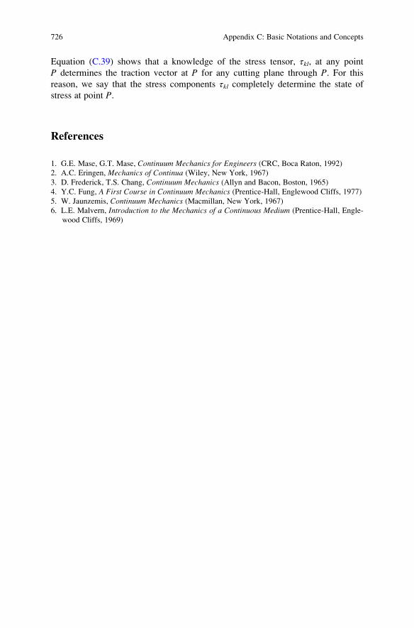
Equation (C.39) shows that a knowledge of the stress tensor, τkl, at any point

P determines the traction vector at P for any cutting plane through P. For thisreason, we say that the stress components τkl completely determine the state of

stress at point P.

References

1. G.E. Mase, G.T. Mase, Continuum Mechanics for Engineers (CRC, Boca Raton, 1992)2. A.C. Eringen, Mechanics of Continua (Wiley, New York, 1967)

3. D. Frederick, T.S. Chang, Continuum Mechanics (Allyn and Bacon, Boston, 1965)

4. Y.C. Fung, A First Course in Continuum Mechanics (Prentice-Hall, Englewood Cliffs, 1977)

5. W. Jaunzemis, Continuum Mechanics (Macmillan, New York, 1967)

6. L.E. Malvern, Introduction to the Mechanics of a Continuous Medium (Prentice-Hall, Engle-

wood Cliffs, 1969)


Appendix D: The Hilbert Transform

The Hilbert transform of a function often occurs in signal processing applications

and in reflection and refraction problems when critical angles are exceeded (see

Chap. 6). It also appears frequently in integral transform theory [1]. Here, we define

the Hilbert transform of the function f(t) as:

f H uð Þ ¼ H f tð Þ; u½ � ¼ 1=π

ðþ1

�1

f tð Þdtt� u

; ðD:1Þ

where the integral is interpreted in the principal value sense, i.e.

limε!0

ðu�ε

�1þ

ðþ1

uþε

0@

1A f tð Þdt

t� u: ðD:2Þ

As with the Fourier transform, there is an inverse Hilbert transform that can recover

f(t) given by

f tð Þ ¼ �1

π

ðþ1

�1

f H uð Þduu� t

: ðD:3Þ

D.1 Properties of the Hilbert Transform

Some of the important properties of the Hilbert transform are given by

1. H f aþ tð Þ; u½ � ¼ H f tð Þ; uþ a½ � ðD:4aÞ



727

http://dx.doi.org/10.1007/978-3-319-30463-2_6

2. H f atð Þ; u½ � ¼ H f tð Þ; au½ � a > 0ð Þ ðD:4bÞ3. H f �atð Þ; u½ � ¼ �H f tð Þ;�au½ � a > 0ð Þ ðD:4cÞ

4. H f0tð Þ; u

h i¼ df H uð Þ

duðD:4dÞ

5. H tf tð Þ; u½ � ¼ u f H uð Þ þ 1=π

ðþ1

�1f tð Þdt ðD:4:eÞ

Hilbert transforms for some commonly occurring functions f(t):

f tð Þ : H f tð Þ; u½ � :

δ tð Þ � 1

πu

H t� t0ð Þ � 1=πð Þln u� t0j j

H t� bð Þ � H t� að Þ 1=πð Þln u� a

u� b

��

tυ�1H tð Þ 0 < Reυ < 1�uð Þυ�1 �1 < u < 0

uυ�1ctg πυð Þ 0 < u < 1

(

sin affiffit

p� �H tð Þ a > 0

exp �affiffiffiu

pð Þ �1 < u < 0

cos affiffiffiu

pð Þ 0 < u < 1

(

cos ωtð Þ ω > 0 � sin ωuð Þ

sin ωtð Þ ω > 0 cos ωuð Þt

t2 þ a2Rea > 0

a

u2 þ a2

a

t2 þ a2Rea > 0 � u

u2 þ a2

References

1. I.H. Sneddon, The Use of Integral Transforms (McGraw-Hill Book Co., New York, 1972)

728 Appendix D: The Hilbert Transform

Appendix E: The Method of Stationary Phase

In wave propagation and scattering models, obtaining explicit analytical results in

many cases is made difficult by the complex interactions present. Usually, expres-

sions can only be reduced to the form of integrals which then must be evaluated

numerically or approximately. This Appendix will consider a method of approxi-

mation that is particularly useful called the method of stationary phase [4, 5].

Basically the method relies on the fact that at high frequencies, where the phase

term in an integrand can be rapidly varying, only certain regions contribute

significantly to the integral. Assuming high frequencies is a relatively mild assump-

tion in many NDE problems since the characteristic lengths involved in most

applications are many wavelengths long. Thus, the method of stationary phase

can often be applied without placing severe restrictions on the validity of the

results.

E.1 Single Integral Forms

Consider the case of a one-dimensional integral of the form

I ¼ðba

f xð Þexp ikϕ xð Þ½ �dx; ðE:1Þ

where the wave number, k, is assumed to be large and f(x) is a smoothly varying

function. Since the phase of the complex exponential will vary rapidly in this case,

with each half period oscillation nearly canceling the adjacent half period oscilla-

tion of opposite sign, we expect that I ! 0 as k ! 1 . Under such circumstances

the major contribution of the integral will come from points where the phase term

ϕ(x) is stationary, i.e. ϕ0xð Þ ¼ dϕ xð Þ=dx ¼ 0. To see this, consider the following

integral:



729

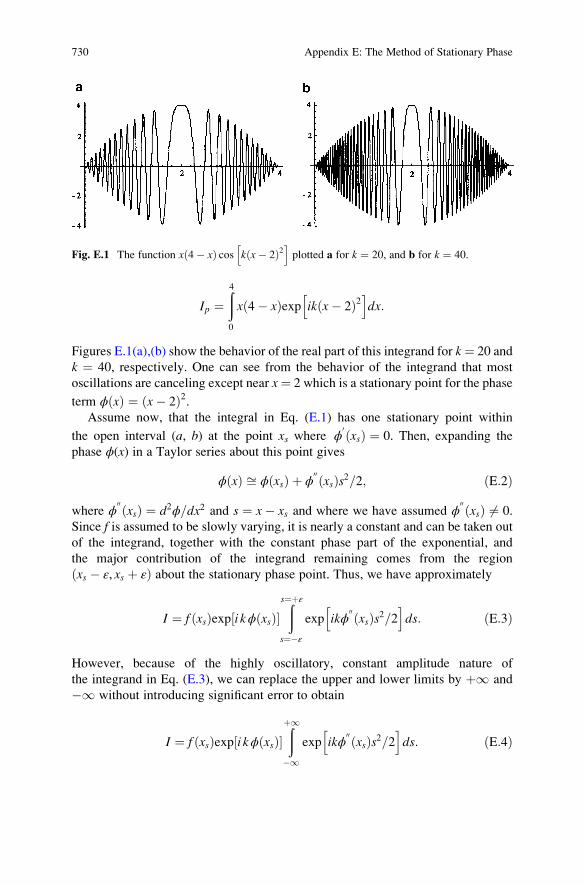
Ip ¼ð40

x 4� xð Þexp ik x� 2ð Þ2h i

dx:

Figures E.1(a),(b) show the behavior of the real part of this integrand for k¼ 20 and

k ¼ 40, respectively. One can see from the behavior of the integrand that most

oscillations are canceling except near x¼ 2 which is a stationary point for the phase

term ϕ xð Þ ¼ x� 2ð Þ2.Assume now, that the integral in Eq. (E.1) has one stationary point within

the open interval (a, b) at the point xs where ϕ0xsð Þ ¼ 0. Then, expanding the

phase ϕ(x) in a Taylor series about this point gives

ϕ xð Þ ffi ϕ xsð Þ þ ϕ00xsð Þs2=2; ðE:2Þ

where ϕ00xsð Þ ¼ d2ϕ=dx2 and s ¼ x� xs and where we have assumed ϕ

00xsð Þ 6¼ 0.

Since f is assumed to be slowly varying, it is nearly a constant and can be taken out

of the integrand, together with the constant phase part of the exponential, and

the major contribution of the integrand remaining comes from the region

xs � ε, xs þ εð Þ about the stationary phase point. Thus, we have approximately

I ¼ f xsð Þexp i kϕ xsð Þ½ �ðs¼þε

s¼�ε

exp ikϕ00xsð Þs2=2

h ids: ðE:3Þ

However, because of the highly oscillatory, constant amplitude nature of

the integrand in Eq. (E.3), we can replace the upper and lower limits by þ1 and

�1 without introducing significant error to obtain

I ¼ f xsð Þexp i kϕ xsð Þ½ �ðþ1

�1exp ikϕ

00xsð Þs2=2

h ids: ðE:4Þ

Fig. E.1 The function x 4� xð Þ cos k x� 2ð Þ2h i

plotted a for k ¼ 20, and b for k ¼ 40.

730 Appendix E: The Method of Stationary Phase

Now, if we let k ϕ00xsð Þ�� s2=2 ¼ t2, it follows that ds ¼ 2=k ϕ

00xsð Þ�� 1=2

dt and the

stationary phase approximation of the integral, Is, is

Is ¼ f xsð Þ 2=k ϕ00xsð Þ�� h i1=2

exp ikϕ xsð Þ½ �ðþ1

�1exp i t2sgn ϕ

00xsð Þ

n oh idt: ðE:5Þ

The integral in Eq. (E.5) can be performed exactly since we have [1]

ðþ1

�1cos t2

� �dt ¼ ffiffiffiffiffiffiffiffi

π=2p

ðþ1

�1sin t2

� �dt ¼ ffiffiffiffiffiffiffiffi

π=2p

;

ðE:6Þ

so that

ðþ1

�1exp it2sgn ϕ

00xsð Þ

n oh idt ¼ 1þ isgn ϕ

00xsð Þ �� ffiffiffiffiffiffiffiffi

π=2p

¼ ffiffiffiπ

pexp iπsgn ϕ

00xsð Þ �

=4� ðE:7Þ

and the integral becomes, finally

Is ¼ 2π=kϕ00xsð Þ

h i1=2f xsð Þexp ikϕ xsð Þ þ iπ sgn ϕ

00xsð Þ

n o=4

h i: ðE:8Þ

Equation (E.8) gives an explicit expression for the stationary phase evaluation of

the original integral when a single isolated stationary phase point exists in the open

interval (a, b). Special cases when multiple stationary phase points exist, or when

the stationary phase point(s) are at the interval end points, and cases where ϕ00 ¼ 0

at the stationary point can also be considered (see [1] for further details). However,

for the specific problems covered in this book, Eq. (E.8) will generally suffice.

The only special case not covered by Eq. (E.8) we would like to consider is when

there is no stationary phase point at all in the closed interval [a, b]. Then we can

write I in the form

I ¼ðba

f xð Þikϕ

0xð Þ

� exp ikϕ xð Þf gikϕ0

xð Þdx; ðE:9Þ

where the second term in square brackets in Eq. (E.9) is a perfect differential so that

an integration by parts gives

Appendix E: The Method of Stationary Phase 731

I ¼ f xð Þexp ikϕ xð Þ½ �ikϕ

0xð Þ

��b

a

� 1

ik

ðba

f xð Þ=ϕ0xð Þ

h i0

exp ikϕ xð Þ½ �dx: ðE:10Þ

Sinceϕ0xð Þ 6¼ 0 in [a, b] we can again write the integral in Eq. (E.10) as the product

of two terms, one being a perfect differential, and perform the integration by parts

again. Thus, keeping only the first terms, for k large we have

I ¼ f bð Þexp ikbð Þikϕ

0bð Þ � f að Þexp ikað Þ

ikϕ0að Þ þ O

1

k2

� �: ðE:11Þ

E.2 Double Integral Forms

In some problems we will encounter two-dimensional integrals similar to

Eq. (E.1), e.g.

I ¼ðb1a1

ðb2a2

f x; yð Þexp ikϕ x; yð Þ½ �dxdy; ðE:12Þ

where again k is large and the function f is assumed to be smoothly varying. We will

assume a stationary phase point exists at the point xs ¼ xs; ysð Þ inside the limits of

the integrals. Then ∂ϕ xsð Þ=∂x ¼ ∂ϕ xsð Þ=∂y ¼ 0 and we can expand ϕ in a Taylor

series to second order as

ϕ x; yð Þ ¼ ϕ xs; ysð Þ þ 1

2ϕ s,xx x� xsð Þ2 þ 2ϕ s

,xy x� xsð Þ y� ysð Þ þ ϕ s,yy y� ysð Þ2

n o;

ðE:13Þ

where ϕ s,xy ¼ ∂2ϕ xsð Þ=∂x∂y,etc. If we change to new coordinates (u, v), where

u ¼ x� xsð Þv ¼ y� ysð Þ þ ϕ s

,xy x� xsð Þ=ϕ s,yy

ðE:14Þ

then dxdy ¼ dudv since the Jacobian, J, of the transformation is given by

J ¼ ∂u=∂x ∂u=∂y

∂v=∂x ∂v=∂y

�� ¼

1 0

ϕ s,xy=ϕ

s,yy 1

��: ðE:15Þ


Also, as can be verified, via the chain rule,

ϕ s,xx x� xsð Þ2 þ 2ϕ s

,xy x� xsð Þ y� ysð Þ þ ϕ s,yy y� ysð Þ2

¼ ϕ s,uuu

2 þ 2ϕ s,uvuvþ ϕ s

,vvv2

ðE:16Þ

and

ϕ s,vv ¼ ϕ s

,yy

ϕ s,uv ¼ 0

ϕ s,uu ¼ ϕ s

,xx � ϕ s,xy

� �2

=ϕ s,yy

ðE:17Þ

so that the original integral, in the u, v coordinates can be approximated, as in the

one-dimensional case, as

Is ¼ f xs; ysð Þexp ikϕ xs; ysð Þ½ �ðþ1

�1

ðþ1

�1exp ik ϕ s

,uuu2 þ ϕ s

,vvv2

� �� dudv: ðE:18Þ

Since the u and v integrals in Eq. (E.18) are identical to the forms we evaluated

previously in the one-dimensional case (see Eq. (E.4)), we can obtain immediately

Is ¼ 2π

k ϕ s,uu

�� " #1=2

2π

k ϕ s,vv

�� " #1=2

f xs; ysð Þ

� exp ikϕ xs; ysð Þ þ iπ sgn ϕ s,uu

�þ sgn ϕ s,vv

�� =4

� ;

ðE:19Þ

which can be written in terms of the original x and y coordinate values by defining

H ¼ ϕ s,uuϕ

s,vv ¼ ϕ s

,xxϕs,yy � ϕ s

,xy

� �2

σ ¼ sgn ϕ s,uu

�þ sgn ϕ s,vv

� ðE:20Þ

and noting that

σ ¼0 if H < 0

2 if H > 0, ϕ s,yy > 0

�2 if H > 0, ϕ s,yy < 0

8><>: ðE:21Þ

so that we have, finally

Is ¼ 2π

k

f xs; ysð Þffiffiffiffiffiffiffiffiffiffiffiffiffiffiffiffiffiffiffiffiffiffiffiffiffiffiffiffiffiffiffiffiffiffiffiffiffiffiffiffiϕ s,xxϕ

s,yy � ϕ s

,xy

� �2��

��s exp ikϕ xs; ysð Þ þ iπσ=4½ �: ðE:22Þ


E.3 Curved Surface Integral

The last case that we will consider by the method of stationary phase is the

evaluation of a particular integral over a curved surface given by

I ¼ðS

f xð Þexp ik a � xð Þ½ �dS xð Þ; ðE:23Þ

where the surface S will be assumed to be smooth, but otherwise arbitrary, and the

vector a, is a constant. Again, we wish to evaluate this integral at high frequencies,

i.e. when k is large. In this case, we have taken the phase term to be of the particular

form ϕ xð Þ ¼ a � x which will occur in a number of applications.

As in the previous cases, we will assume the major contribution to this integral

comes from the evaluation near a stationary phase point xs on the surface. We can

parameterize S in terms of two surface coordinates (t1, t2) so that on S we can write

x ¼ x t1; t2ð Þ. Then in this case the stationary phase conditions become

∂ϕ=∂t1 ¼ ∂ϕ=∂t2 ¼ 0

or, explicitly

a � ∂x=∂t1 ¼ 0

a � ∂x=∂t2 ¼ 0:ðE:24Þ

Since the vectors ∂x=∂tα α ¼ 1, 2ð Þ are tangent to the surface, it follows from

stationary phase that at the stationary phase point xs ¼ b1; b2ð Þ, a is parallel to the

unit normal, nI, which is taken here to be the inward normal. Then, expanding ϕ in a

Taylor series about the stationary phase point as before, we obtain in this case

ϕ ¼ a � x t1; t2ð Þ ¼ a � xs þ 1

2tα � bαð Þ tβ � bβ

� �a � x s

,αβ

n o; ðE:25Þ

wherex s,αβ ¼ ∂2

x b1; b2ð Þ=∂tα∂tβ Then, the integral can be written approximately as

I ¼ f xsð Þexp ika � xsð ÞJ xsð Þðb2þε2

b2�ε2

ðb1þε1

b1�ε1

exp1

2k tα � bαð Þ tβ � bβ

� �a � x s

,αβ

n o� dt1dt2;

ðE:26Þwhere dS ¼ Jdt1dt2 is the area element in the (t1, t2) coordinates and J is a Jacobian.From differential geometry [3] we have

x s,αβ ¼ Γ γ

αβ xsð Þx s, γ þ hαβ xsð ÞnI xsð Þ: ðE:27Þ


where Γγαβ are Christoffel’s symbols of the second kind, hαβ is the curvature tensor,

and x s, γ ¼ ∂x b1; b2ð Þ=∂tγ . The dot product of a with these second order partial

derivatives of the position vector can be expressed in general as

a � x s,αβ ¼ Γ γ

αβ xsð Þ a � x s, γ

� �þ hαβ xsð Þ a � nI xsð Þ� �

: ðE:28Þ

However, from the stationary phase conditions the first term on the right side of

Eq. (E.27) vanishes, leaving

a � x s,αβ ¼ hαβ xsð Þ a � nI xsð Þ� �

: ðE:29Þ

If t1 and t2 are chosen in particular to be the arc length parameters taken along the

principal directions of the surface at xs, then

h12 xsð Þ ¼ h21 xsð Þ ¼ 0

h11 xsð Þ ¼ κ1

h22 xsð Þ ¼ κ2

ðE:30Þ

and J xsð Þ ¼ 1 where κ1 and κ2 are the principal curvatures of the surface at xs andthe stationary phase contribution to the integral becomes (expanding the limits of

integration, as before to infinity):

Is ¼ f xsð Þexp i ka � xs½ �

ðþ1

�1

ðþ1

�1exp

1

2ka � nI xsð Þ κ1 t1 � b1ð Þ2 þ κ2 t2 � b2ð Þ2

n oh idt1 dt2:

ðE:31Þ

With this choice of coordinates the integrals appearing in Eq. (E.31) can be

independently evaluated since they are in the same general form as found in the

one- and two-dimensional integral cases considered previously. Thus, we find

Is ¼ 2π

k κ1a � nI xsð Þj j� 1=2

2π

k κ2a � nI xsð Þj j� 1=2

f xsð Þexp ika � xs þ iπσ=4½ �; ðE:32Þ

where

σ ¼ sgn κ1 a � nI xsð Þ �þ sgn κ2 a � nI xsð Þ �� : ðE:33Þ

If we let

κ1j j ¼ 1=R1

κ2j j ¼ 1=R2;ðE:34Þ


where R1 and R2 are the magnitudes of the principal radii of curvature of S at xs,

we have

Is ¼ 2πffiffiffiffiffiffiffiffiffiffiR1R2

pk a � nI xsð Þj j f xsð Þexp i ka � xs þ iπσ=4½ �: ðE:35Þ

References

1. I.S. Gradshteyn and I.M. Ryzhik, Table of Integrals, Series, and Products (Academic,

New York, 1980)

2. L.B. Felsen, N. Marcuvitz, Radiation and Scattering of Waves (Prentice-Hall, Inglewood

Cliffs, 1973)

3. I.S. Sokolnikoff, Tensor Analysis, 2nd edn. (Wiley, New York, 1964)

4. N. Bleistein, R.A. Handelsman, Asymptotic Expansion of Integrals (Dover Publications,

New York, 1986)

5. N. Bleistein, Mathematical Methods for Wave Phenomena (Academic, New York, 1984)


Appendix F: Properties of Ellipsoids

F.1 Geometry of an Ellipsoid

In Chap. 10, it was shown that the far field scattering response of ellipsoidal

inclusions and elliptical cracks can be obtained explicitly through the use of the

Born and Kirchhoff approximations. These same approximations were used in

Chap. 15 to develop a number of equivalent flaw sizing algorithms. In this Appen-

dix, we will derive some of the geometrical properties of ellipsoids that are useful in

such applications. The details discussed here can also be typically found in texts on

tensor analysis and differential geometry [1–3].

One geometrical quantity that appears frequently in Chaps. 10 and 15 is the

effective radius of an ellipsoid, re, which was defined to be the perpendicular

distance from the center of an ellipsoid to a plane P which is tangent to its surface

at some point, x0, as shown in Fig. F.1. If we write the equation of the ellipsoid as

g x1; x2; x3ð Þ ¼ x21a21

þ x22a22

þ x23a23

� 1 ¼ 0; ðF:1Þ

then since the unit outward normal, n, is given by n ¼ ∇g= ∇gj j its components are

n1 ¼ x1Ha21

, n2 ¼ x2Ha22

, n3 ¼ x3Ha23

ðF:2Þ

with

H ¼ffiffiffiffiffiffiffiffiffiffiffiffiffiffiffiffiffiffiffiffiffiffiffiffiffix21a41

þ x22a42

þ x23a43

s: ðF:3Þ

If a plane P, whose unit normal is ei touches and is tangent to the ellipsoid at

the point x0 ¼ x01; x02; x

03

� �, then ei coincides with the unit normal at this point, i.e.

ei ¼ n x01; x02; x

03

� � ¼ n0 and for any point X in this plane we may write



737

http://dx.doi.org/10.1007/978-3-319-30463-2_10

http://dx.doi.org/10.1007/978-3-319-30463-2_15

http://dx.doi.org/10.1007/978-3-319-30463-2_10

http://dx.doi.org/10.1007/978-3-319-30463-2_15

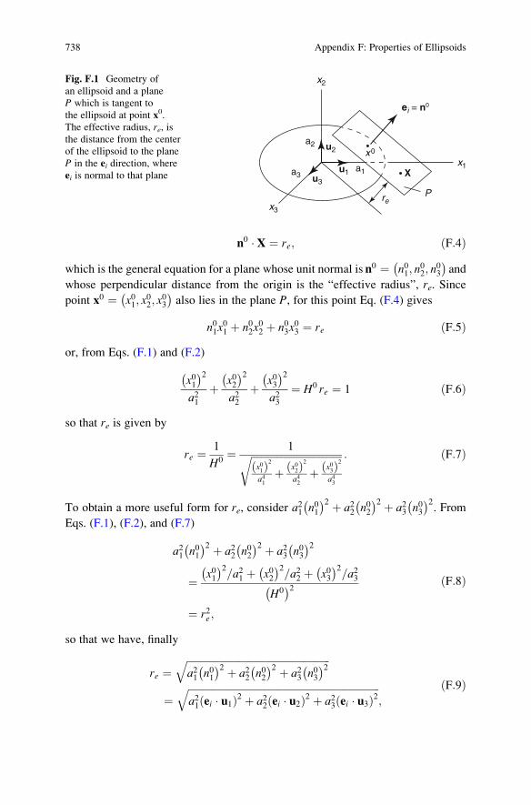
n0 � X ¼ re; ðF:4Þwhich is the general equation for a plane whose unit normal is n0 ¼ n01; n

02; n

03

� �and

whose perpendicular distance from the origin is the “effective radius”, re. Since

point x0 ¼ x01; x02; x

03

� �also lies in the plane P, for this point Eq. (F.4) gives

n01x01 þ n02x

02 þ n03x

03 ¼ re ðF:5Þ

or, from Eqs. (F.1) and (F.2)

x01� �2a21

þ x02� �2a22

þ x03� �2a23

¼ H0 re ¼ 1 ðF:6Þ

so that re is given by

re ¼ 1

H0¼ 1ffiffiffiffiffiffiffiffiffiffiffiffiffiffiffiffiffiffiffiffiffiffiffiffiffiffiffiffiffiffiffiffiffiffiffiffi

x01ð Þ2a41

þ x02ð Þ2a42

þ x03ð Þ2a43

r : ðF:7Þ

To obtain a more useful form for re, consider a21 n01� �2 þ a22 n02

� �2 þ a23 n03� �2

. From

Eqs. (F.1), (F.2), and (F.7)

a21 n01� �2 þ a22 n02

� �2 þ a23 n03� �2

¼ x01� �2

=a21 þ x02� �2

=a22 þ x03� �2

=a23

H0� �2

¼ r2e ;

ðF:8Þ

so that we have, finally

re ¼ffiffiffiffiffiffiffiffiffiffiffiffiffiffiffiffiffiffiffiffiffiffiffiffiffiffiffiffiffiffiffiffiffiffiffiffiffiffiffiffiffiffiffiffiffiffiffiffiffiffiffiffiffiffiffiffiffia21 n01� �2 þ a22 n02

� �2 þ a23 n03� �2q

¼ffiffiffiffiffiffiffiffiffiffiffiffiffiffiffiffiffiffiffiffiffiffiffiffiffiffiffiffiffiffiffiffiffiffiffiffiffiffiffiffiffiffiffiffiffiffiffiffiffiffiffiffiffiffiffiffiffiffiffiffiffiffiffiffiffiffiffiffiffiffiffiffiffiffiffiffia21 ei � u1ð Þ2 þ a22 ei � u2ð Þ2 þ a23 ei � u3ð Þ2

q;

ðF:9Þ

a3a1

reP

X

x2

x3

x1

x0

ei = n0

a2 u2

u3

u1

Fig. F.1 Geometry of

an ellipsoid and a plane

P which is tangent to

the ellipsoid at point x0.The effective radius, re, isthe distance from the center

of the ellipsoid to the plane

P in the ei direction, whereei is normal to that plane

738 Appendix F: Properties of Ellipsoids

where (u1, u2,u3) are unit vectors along the axes of the ellipsoid (Fig. F.1). Thus, if

we are given the normal to the plane, ei, and the size and orientation of the ellipsoid

through the parameters (a1, a2, a3) and (u1,u2, u3), respectively, Eq. (F.9) deter-mines the effective radius. Also, the point where the plane touches the ellipsoid can

then be obtained, since

x01 ¼ a21n01=re

x02 ¼ a22n02=re

x03 ¼ a23n03=re:

ðF:10Þ

Finally, it is interesting to note that Eqs. (F.2), (F.4), and (F.6) also imply that an

equivalent form for the plane P is given by

x01X1

a21þ x02X2

a22þ x03X3

a23¼ 1: ðF:11Þ

which is a result commonly derived in differential geometry texts.

As shown in Chap. 15, measurements of an effective radius of an unknown flaw

from different directions allows one to use Eq. (F.9) to obtain the equivalent

ellipsoidal size and orientation parameters for that flaw. Thus, Eq. (F.9) is the key

geometrical relationship for performing equivalent flaw sizing.

Another geometrical parameter that appeared in the leading edge response of

ellipsoids in Chap. 10 was the Gaussian curvature of the ellipsoid. To obtain an

expression for this curvature, we parameterize the surface of the ellipsoid by two

parameters (t1, t2) as follows:

x1 ¼ a1 cos t1 cos t2

x2 ¼ a2 cos t1 sin t2

x3 ¼ a3 sin t1:

ðF:12Þ

Then, any point x on the ellipsoid is given by

x ¼ a1 cos t1 cos t2 u1 þ a2 cos t1 sin t2 u2 þ a3 sin t1 u3: ðF:13Þ

From differential geometry the mean and Gaussian curvatures, M and K, respec-tively, of a surface are given by [1]

M ¼ g11h22 þ g22h11 � 2g12h12

2 x, 1 x, 2j j2

K ¼ h11h22 � h212x, 1 x, 2j j2 ;

ðF:14Þ

Appendix F: Properties of Ellipsoids 739

http://dx.doi.org/10.1007/978-3-319-30463-2_15

http://dx.doi.org/10.1007/978-3-319-30463-2_10

where gαβ and hαβ are the first and second fundamental forms

gαβ ¼ x, α � x, βhαβ ¼ nI � x, αβ

ðF:15Þ

and the comma denotes partial differentiation with respect to the t parameters, i.e.

x, α ¼ ∂x=∂tα, etc. The vector nI is the inward unit normal to the ellipsoid which is

given parametrically from Eqs. (F.2), (F.7), and (F.12) as

nI ¼ �rea1

cos t1 cos t2 u1 � rea2

cos t1 sin t2 u2 � rea3

sin t1 u3: ðF:16Þ

Placing the x and nI expressions into Eq. (F.15), we obtain explicitly

g11 ¼ x, 1 � x, 1 ¼ a21 sin2t1 cos

2t2 þ a22 sin2t1 sin

2t2 þ a23 cos2t1

g12 ¼ x, 1 � x, 2 ¼ a21 � a22� �

sin t1 cos t1 sin t2 cos t2

g22 ¼ x, 2 � x, 2 ¼ a21 sin2t2 þ a22 cos

2t2� �

cos 2t1

h11 ¼ nI � x, 11 ¼ re

h12 ¼ nI � x, 12 ¼ 0

h22 ¼ nI � x, 22 ¼ re cos2t1

ðF:17Þ

from which the mean and Gaussian curvatures can be computed at x0 from

Eq. (F.14) as

M ¼ κ1 þ κ22

¼ re2a21a

22a

23

a21 a22 þ a23� �

ei � u1ð Þ2 þ a22 a21 þ a23� �n

ei � u1ð Þ2

þ a23 a21 þ a21� �

ei � u3ð Þ2o ðF:18Þ

and

K ¼ κ1κ2 ¼ 1

R1R2

¼ r4ea21a

22a

23

; ðF:19Þ

where κ1 and κ2 are the principal curvatures of the ellipsoid and R1 and R2 are the

corresponding principal radii of curvature. Just as the Gaussian curvature appears in

the first order leading edge response of volumetric flaws, Chen [4] has shown that

the mean curvature also appears in a higher order expansion of this leading edge

expression.

740 Appendix F: Properties of Ellipsoids

References

1. I. Sokolnikoff, Tensor Analysis, 2nd Ed., (Wiley, New York, 1964)

2. J. McConnell, Applications of the Absolute Differential Calculus (Blackie and Son, London,

1936 (Dover reprint))

3. D. Struick, Lectures on Differential Geometry (Wiley\Interscience, New York, 1969)

4. J.S. Chen, Elastodynamic ray theory and asymptotic methods for direct and inverse scattering

problems, (Ph.D. Thesis (unpublished), Iowa State University, 1987)

Appendix F: Properties of Ellipsoids 741

Appendix G: Matlab Functions and Scripts

In this second edition, MATLAB® functions and scripts have been included to

implement some of the ultrasonic models we have considered. This Appendix

briefly describes those functions and scripts. Additional MATLAB models for a

variety of ultrasonic NDE problems are also available in two related books:

L.W. Schmerr and S.J. Song, Ultrasonic Nondestructive Evaluation Systems –

Models and Measurements, Springer, 2007, and L.W. Schmerr, Fundamentals of

Ultrasonic Phased Arrays, Springer, Springer, 2015. The MATLAB code listings

for this book are available on the web from the publisher or they can be obtained

directly by sending an email with the subject title “Ultrasonic NDE Codes” to the

author at [email protected].

G.1 Transmission and Reflection of Plane Waves

fluid_fluid

>> [R, T] ¼ fluid_fluid(iangd, d1, d2, c1, c2). A function which returns

(R,T) the reflection and transmission coefficients (based on velocity

ratios) for a plane wave incident on a plane interface between two fluids

at an angle iangd (in degrees).The parameters (d1,c1) and (d2, c2) are

the densities and wave speeds in the first and second fluids. The units of

these quantities are arbitrary but must be consistent.

fluid_solid

>> [tpp, tps] ¼ fluid_solid(iangd, d1, d2, cp1, cp2, cs2). A function

which returns (tpp, tps) the plane wave transmission coefficients for a

P-wave and S-wave, respectively, produced in a solid at a fluid-solid

interface due to a P-wave incident in the fluid at an angle iangd

(in degrees). The coefficients are both based on velocity ratios. The

parameters (d1, cp1) are the density and wave speed of the fluid and (d2,



743

[email protected]/

cp2, cs2) are the density, P-wave speed, and S-wave speed, respec-

tively. The units of these quantities are arbitrary but must be

consistent.

solid_f_solid

>> [tpp, tps] ¼ solid_f_solid(iangd, d1, d2, cp1, cs1, cp2, cs2). A

function which returns the P-P(tpp)and P-S(tps) transmission coeffi-

cients, based on velocity ratios, for a P-wave incident on a plane

interface between two solids that are in smooth contact through an

intermediate fluid layer of zero thickness. The parameters (d1, cp1,

cs1) are the density, P-wave speed, and S-wave speed for the first solid

while (d2, cp2, cs2) are the corresponding parameters for the second

solid. The units of these parameters are arbitrary but must be

consistent.

solid_solid

>> [tp, ts, rp, rs] ¼ solid_solid(iangd, d1, d2, cp1, cs1, cp2, cs2,

type). A function which returns the transmitted P-wave (tp), transmit-

ted SV-wave (ts), reflected P-wave (rp), and reflected SV-wave

(rs) transmission/reflection coefficients (based on velocity ratios)

for two solids in welded contact. The inputs are the incident angle

(s),iangd,(in degrees), (d1, d2), the densities of the two media,

(cp1, cs1), the compressional and shear wave speeds of the first medium,

and (cp2, cs2) the compressional and shear wave speeds of the second

medium. The parameter type is a string,(’P’ or ’S’), which indicates the

type of incident wave in medium one. If cs1¼0 and type¼ ’P’ the function

returns the coefficients for a fluid-solid interface with rs ¼ 0. The wave

speed cs2 cannot be set equal to zero.

stress_freeP

>> [Rp, Rs] ¼ stress_freeP(ang, cp, cs). A function which returns (Rp,

Rs),the reflection coefficients for the reflected P-waves and S-waves,

respectively,(based on velocity ratios)for a plane P-wave incident on

a plane stress-free surface of an elastic solid. The parameter ang is

the incident angle (in degrees), cp, cs are the P- and S-wave speeds,

respectively, and. The units of the wave speeds are arbitrary but must

be consistent. Note that there are no critical angles for this case.

snells_law

>> [ang_in, ang_out]¼ snells_law(ang, c1, c2, type). A function which

returns (ang_in, ang_out) the incident and refracted angle at a plane

interface, respectively,(in degrees)that satisfy Snell’s law. The

first input, ang, is a given incident or refracted angle, ang,

(in degrees) that a travelling wave makes with respect to the normal of

a plane interface. The wave speed in the first medium is c1 and the wave

speed in the second medium is c2. The input parameter, type, is either

the string ’f’ or the string ’r’, indicating a forward or reverse,

744 Appendix G: Matlab Functions and Scripts

problem, respectively. For a forward problem ang is taken as the inci-

dent angle and the refracted angle is calculated. For a reverse problem

ang is taken to be the refracted angle and the incident angle is calcu-

lated. The angle argument, ang, must be in the range 0 <¼ ang <¼90 degrees.

G.2 Surface and Plate Waves

Rayleigh_speed

>> cr ¼ Rayleigh_speed(cp, cs). A function which returns the Rayleigh

wave speed, cr, at a free surface of a solid where (cp, cs) are the P-wave

and S-wave speeds, respectively. The units of the wave speeds are arbi-

trary but must be consistent.

dispersion_plots

>> dispersion_plots. A script which creates a 2-D set of normalized

frequency and wave speed values at which the Rayleigh-Lamb dispersion

function for symmetrical or anti-symmetrical plate waves is evaluated.

The MATLAB function contour is then used to plot the dispersion curves

for this 2-D region. Note that the fundamental anti-symmetrical mode

plot is unreliable at very small frequencies and must be replaced by the

analytical results for this mode at those values.

Rayleigh_LambM

>> y¼ Rayleigh_LambM(c, cp, cs, fh, type). A function which returns the

Rayleigh-Lamb function values for symmetrical or unsymmetrical plate

waves. The input parameter, c, is the wave speed of the plate wave, while

(cp, cs) are the compressional and shear wave speeds of the plate,

respectively. The wave speed values are arbitrary but must be consis-

tent. The parameter fh is the frequency times the half width of the

plate. The input parameter, type, is a string,(’s’ or ’a’)for symmet-

rical or ant-symmetrical modes, respectively.

dispersion_curves

>> dispersion_curves. A script, which like the script

dispersion_plots, generates a 2-D set of non-dimensional frequency

and wave speed values at which the plate wave Rayleigh-Lamb dispersion

function is evaluated for symmetrical or anti-symmetrical plate waves.

The dispersion curves are then plotted with the MATLAB function con-

tour. Individual dispersion curves are extracted and ordered in fre-

quency. The fundamental flexural mode values for small frequencies where

the contour values are unreliable are modified with analytical results.

The specific dispersion curve specified by the user is then plotted.

Appendix G: Matlab Functions and Scripts 745

G.3 Ultrasonic Beam Models

bdw_fluid

>> p ¼ bdw_fluid(x, y, z, a, c, f, N). A function which returns the

normalized pressure, p, for a planar circular piston transducer of

radius, a,(in mm), radiating into a fluid of wave speed, c, (in m/sec),

at a frequency, f,(in MHz). The pressure is calculated at the points (x,

y, z) (in mm), where (x, y, z) can be scalars, vectors, or matrices. N, is

an optional input parameter that specifies the number of line segments

used to approximate the edge integral in a boundary diffraction wave

model. If N is not specified, N is determined automatically so that the

line segment length is no larger than one tenth of a wavelength. This

function calls the supporting function bdw_model which implements the

boundary diffraction wave model of the transducer.

bdw_model

>> p ¼ bdw_model(rho, z, a, c, f, N). A function which returns the nor-

malized pressure, p, for a circular transducer of radius, a,(in mm),

radiating into a fluid of wave speed, c, (in m/sec), at a frequency, f,

(in MHz). The pressure is calculated at the radial distance rho(in mm)

and axial distance, z,(in mm) in the fluid. N is the number of line seg-

ments used to approximate the edge integral in a boundary diffraction

wave model. All input parameters must be scalars. This is a supporting

function which called multiple times by the function bdw_fluid.

onaxis_foc

>> p ¼ onaxis_foc(z, f, a, R, c). A function which calculates the

on-axis normalized pressure,p, at the locations z(in mm)of a spheri-

cally focused transducer of radius a (in mm) and focal length R(in mm)

radiating into a fluid with wave speed c(in m/sec), using the O’Neil

model. If R ¼ inf, the function returns the on-axis pressure of a planar

transducer of radius a.

parameters2

>> parameters2. A script which is used to define the input parameters

needed to model a planar or focused circular piston transducer radiat-

ing through a curved interface. These parameters are then placed in a

MATLAB structure called setup.

gauss_c15

>> [A, B] ¼ gauss_c15(). A function which returns the 15 "optimized"

coefficients obtained by Wen and Breazeale to simulate the wave field of a

circular planar piston transducer radiating into a fluid by a superpo-

sition of Gaussian beams: Wen, J.J. and M. A. Breazeale," Computer

optimization of the Gaussian beam description of an ultrasonic field,"

Computational Acoustics, Vol.2, D. Lee, A. Cakmak, R. Vichnevetsky,

Eds. Elsevier Science Publishers, Amsterdam, 1990, pp. 181-196.


MG_beam2

>> v ¼ MG_beam2(setup). A function which returns the normalized veloc-

ity amplitude, v, due to a planar or spherically focused piston trans-

ducer radiating obliquely through a curved fluid-solid or a smooth

solid-solid interface where the plane of incidence must be aligned

with one of the principal axes of the curved surface. The input parame-

ter setup is a MATLAB structure that is generated by the MATLAB script

parameters2 and contains all of the input parameters needed to define a

given inspection. This is a multi-Gaussian beam model that uses the

15 optimized coefficients of Wen and Breazeale to calculate the wave

field. Those coefficients are returned by the MATLAB function gauss_c15.

onaxis_interface

>> [v, vp] ¼ onaxis_interface(z1, z2, f, a, d1, d2, cp1, cp2, cs2). A

function which computes the on-axis velocity of a circular piston

transducer of radius a (in mm)radiating at a frequency f (in MHz)

through a planar fluid-solid interface at normal incidence. The dis-

tances z1, z2 (in mm) are in the fluid and solid, respectively, whose

densities are d1, d2. The compressional wave speed of the fluid is cp1

and the compressional and shear wave speeds of the solid are cp2, cs2.

All the wave speeds are measured in m/sec. The units of the densities are

arbitrary but must be consistent. The function returns both the normal-

ized on-axis velocity, v, and the corresponding paraxial approxima-

tion, vp, for the on-axis velocity of the transmitted P-wave. The

distance z1 in the fluid must be a scalar.

angle_beam2

>> angle_beam2. A script which generates an image of the wave field of a

45 degree angle beam shear wave transducer in the plane of incidence.

The script uses the multi-Gaussian beam model MG_beam2.

pulse2

>> pulse2. A script which generates a wave form at an on-axis point in

water produced by a circular planar transducer. It uses the multi-Gauss-

ian beam model MG_beam2 and the function spectrum to generate the pulse.

G.4 Flaw Scattering Models

A_crack_pe

>>A¼A_crack_pe(f,b,c,angd).Afunctionwhichreturnsthepulse-echo

scattering amplitude,A, (in mm)for a circular crack of radius b (in mm)

at a frequency,f, (in MHz) in a material with a wave speed, c, (in m/sec)

and at an angle angd(in degrees) using the Kirchhoff approximation.


A_void_pe

>> A ¼ A_void_pe(f, b, c). A function which returns the pulse-echo

scattering amplitude, A,(in mm) of a spherical void of radius b (in mm)

at frequency f (in MHz) in a solid or fluid with wave speed c (in m/sec)

using the Kirchhoff approximation.

A_incl_pe

>> A ¼ A_incl_pe(f,b,c1,d1,c0,d0). A function which calculates the

pulse-echo scattering amplitude, A,(in mm) for a spherical inclusion

of radius b (in mm) where (c1, d1) and (c0, d0) are the wave speeds and

densities of the flaw and host materials, respectively. Wave speeds are

in m/sec and densities are in arbitrary but consistent units. The func-

tion uses the modified Born approximation where the wave travels in the

flaw at the flaw wave speed and the amplitude of the front and back

responses are in terms of the reflection coefficient without making the

weak scattering approximation. A phase correction puts the front and

back responses at the correct times.

sphere_rigid_pe

>> A¼ sphere_rigid_pe(f, b, c). A function which calculates the pulse-

echo scattering amplitude, A, (in mm) for a rigid sphere of radius b

(in mm) in a fluid with wave speed, c, (in m/sec). This function uses the

method of separation of variables.

G.5 Effective Parameters and Flaw Sizing

eff_parameter

>> [aeff, Reff] ¼ eff_parameters(c, f, zmin, zmax). A function which

computes the effective radius (aeff) and effective focal length (Reff)

of a spherically focused transducer from measurements of zmin and zmax

(both in mm),the on-axis min and max locations in the frequency domain

response of the transducer, at a frequency f (in MHz) where the wave

speed c is in meters/sec. If zmax is not specified, then Reff ¼ inf (pla-

nar transducer) is returned and only aeff is calculated. This function

calls a supporting function, transeq.

transeq

>> y ¼ transeq(x, zmax, zmin, k). A function which returns the values y

of the equation y ¼ f(x, zmin, zmax, k), where (zmin, zmax) are measured

values (in mm)of the on-axis min and max response of a focused trans-

ducer and k is the wave number (in rad/mm). The function f is a supporting

function needed to determine the effective parameters of a spherically

focused transducer.


ellipse_data

>> [theta, phi, dt] ¼ ellipse_data(). A function which returns exper-

imental sizing data for a 2.5 x 0.6 mm elliptical crack in titanium(c ¼6100 m/sec) as measured with a phased array where (theta, phi) are the

spherical angles (in degrees) at which dt is measured, where dt is the

time between flash points (in microseconds). These measured values are

corrected for finite bandwidth errors.

K_sizing

>> [pds, a] ¼ K_sizing(c, theta, phi, dt). A function which returns

matrices containing the direction cosines, pds, and lengths of the

semi-major axes,a,(in mm)of an equivalent flat elliptical crack in a

solid with wave speed,c, (in mm/microsec), based on measured times

between flashpoints, dt, (in microsec) at the spherical angles angles

(theta, phi), measured in degrees.

G.6 Miscellaneous Functions

FourierT

>> y ¼ FourierT(x, dt). A function which returns y, the forward FFT of

the sampled time domain values,x, where dt is the sampling time interval

between points. FourierT approximates the Fourier transform where the

integrand of the transform is x*exp(2*pi*i*f*t). This is consistent

with the definition of the forward Fourier transform used in this book.

For NDE applications the frequency components, f, are normally in MHz,

and the sampling time, dt, in microseconds. The values, y, are complex

while the values of x are real.

IFourierT

>> y ¼ IFourierT(x, dt). A function which computes the inverse FFT of

the sampled frequency domain values, x, for a sampling time interval

dt. IFourierT assumes the integrand of the inverse transform is given by

x*exp(-2*pi*i*f*t). This is consistent with the definition of the

inverse Fourier transform used in this book. The first half of the sam-

pled values of x are the spectral components for positive frequencies

ranging from 0 to the Nyquist frequency 1/(2*dt). The second half of the

sampled values are the spectral components for the corresponding neg-

ative frequencies. The values, y, should be real but may contain small

imaginary parts from numerical round off, which can be eliminated by

taking the real part, i.e. real(y).If the negative frequency values are

set equal to zero then to recover the inverse FFT of x we must replace x

(1) by x(1)/2 and then compute 2*real(IFourierT(x,dt)).


s_space

>> y ¼ s_space(xstart, xend, num). A function which generates num

evenly spaced sampled values from xstart to (xend - dx), where dx is the

sample spacing. This is useful in FFT analysis where we generate sampled

periodic functions. Example: generate 1000 sampled frequencies from

0 to 100MHz via f ¼ s_space(0,100,1000); in this case the last value of

f will be 99.9 MHz and the sampling interval will be 100/1000 ¼0.1 MHz.

c_shift

>> y¼ c_shift(x, n). A function which moves the last n components of the

vector x into the first n component places and shifts the remaining com-

ponents of x to follow those n components, i.e. this is a circular shift.

It can be used to prevent a periodic function, as found in FFT analyses,

from being split into the first and last parts of the window in which it is

displayed. Note: x must be a row vector.

t_shift

>> y ¼ t_shift(x, n). A function which is used in conjunction with the

c_shift function to change the time axis values appropriately so that

the time axis is shifted along with the function. Example use: plot

(t_shift(t, 100), c_shift(fun, 100))

spectrum

>> V ¼ spectrum(f, B, fc, bw). A function which returns a Gaussian-

shaped spectrum, V, for a pulse whose time domain waveform is given by

v ¼ B*cos(2*pi*fc*t)*exp(-t^2/4a^2), where fc is the center frequency

(in MHz when t is in microseconds), and bw is the -6dB bandwidth (in MHz).

Note that this is a function defined only for positive frequencies so to

recover the real time domain waveform, v, we must let V(1) ¼ V(1)/2, and

take twice the real part of the inverse FFT.

lp_filter

>> y ¼ lp_filter(f, fstart, fend). A function which returns low-pass

filter, y, at the frequencies contained in the vector f. The filter has

values of 1.0 below the frequency value fstart and tapers to zero at

frequencies above the value fend with a cosine function. An error is

returned if fend is outside the range of values contained in the vector f

or if fend is less than fstart.

display_struct

>> display_struct(setup). A function which returns all the parameters

contained in the structure, setup, where setup is generated by the

script parameters2.

sphH

>> y ¼ sphH(n,x). A function which returns the spherical Hankel func-

tion of order n at x, where x is a non-dimensional argument. It is used in

separation of variables solutions.


sphJ

>> y ¼ sphJ(n,x). A function which returns the spherical Bessel func-

tion of order n at x, where x is a non-dimensional argument. It is used in

separation of variables solutions.


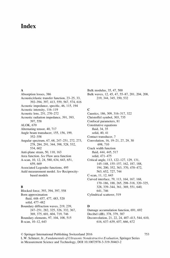
Index

AAbsorption losses, 386

Acoustic/elastic transfer function, 23–25, 33,

392–394, 397, 413, 559, 567, 574, 616

Acoustic impedance, specific, 46, 115, 194

Acoustic intensity, 116–119

Acoustic lens, 251, 270–272

Acoustic radiation impedance, 391, 393,

397, 558

ALOK, 670

Alternating tensor, 40, 717

Angle beam transducer, 155, 156, 199,

352–358

Angular spectrum, 67, 68, 247–251, 272, 273,

278, 284, 291, 344, 398, 528, 532,

534, 602

Anti-plane strain, 50, 110, 163

Area function. See Flaw area function

A-scan, 10, 12, 24, 580, 634, 643, 651,

659, 669

Associated Legendre functions, 495

Auld measurement model. See Reciprocity-based models

BBlocked force, 393, 394, 397, 558

Born approximation

fluid, 448–457, 477, 483, 520

solid, 477–482

Boundary diffraction waves, 219, 239,

247–251, 282, 325, 326, 332, 367,

369, 375, 601, 604, 719, 746

Boundary elements, 97, 104, 108, 515

B-scan, 10–12, 643

Bulk modulus, 35, 47, 500

Bulk waves, 12, 45, 47, 55–87, 201, 204, 208,

219, 344, 345, 350, 532

CCaustics, 186, 309, 316–317, 322

Christoffel symbol, 303, 735

Confocal parameters, 81

Constitutive equations

fluid, 34, 35

solid, 40, 41

Contact transducer, 7

Convolution, 16, 19–21, 27, 29, 30

698, 710

Crack width function

fluid, 444, 445, 517

solid, 471–475

Critical angle, 113, 122–127, 129, 131,

145–148, 155–157, 162, 187, 188,

194, 200, 352, 363, 370, 470–472,

563, 652, 727, 744

C-scan, 11, 12, 643

Curved interface, 79, 113, 164, 167, 168,

170–186, 188, 265, 298–318, 320–325,

328, 339–344, 361, 369, 551, 640,

641, 746

Cylindrical scatterer, 519

DDamage accumulation function, 691, 692

Decibel (dB), 378, 379, 387

Deconvolution, 21, 22, 24, 407–413, 544, 610,

616, 637–639, 657, 666, 672



753

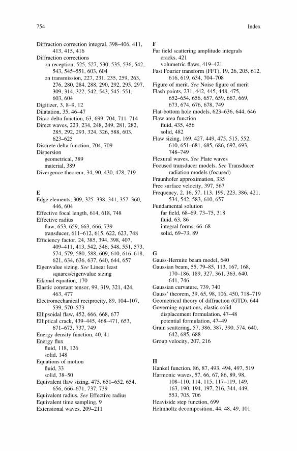
Diffraction correction integral, 398–406, 411,

413, 415, 416

Diffraction corrections

on reception, 525, 527, 530, 535, 536, 542,

543, 545–551, 603, 604

on transmission, 227, 231, 235, 259, 263,

276, 280, 284, 288, 290, 292, 295, 297,

309, 314, 322, 542, 543, 545–551,

603, 604

Digitizer, 3, 8–9, 12

Dilatation, 35, 46–47

Dirac delta function, 63, 699, 704, 711–714

Direct waves, 223, 234, 248, 249, 281, 282,

285, 292, 293, 324, 326, 588, 603,

623–625

Discrete delta function, 704, 709

Dispersion

geometrical, 389

material, 389

Divergence theorem, 34, 90, 430, 478, 719

EEdge elements, 309, 325–338, 341, 357–360,

446, 604

Effective focal length, 614, 618, 748

Effective radius

flaw, 653, 659, 663, 666, 739

transducer, 611–612, 615, 622, 623, 748

Efficiency factor, 24, 385, 394, 398, 407,

409–411, 413, 542, 546, 548, 551, 573,

574, 579, 580, 588, 609, 610, 616–618,

621, 634, 636, 637, 640, 644, 657

Eigenvalue sizing. See Linear leastsquares/eigenvalue sizing

Eikonal equation, 170

Elastic constant tensor, 99, 319, 321, 424,

463, 477

Electromechanical reciprocity, 89, 104–107,

539, 570–573

Ellipsoidal flaw, 452, 666, 668, 677

Elliptical crack, 439–445, 468–471, 653,

671–673, 737, 749

Energy density function, 40, 41

Energy flux

fluid, 118, 126

solid, 148

Equations of motion

fluid, 33

solid, 38–50

Equivalent flaw sizing, 475, 651–652, 654,

656, 666–671, 737, 739

Equivalent radius. See Effective radiusEquivalent time sampling, 9

Extensional waves, 209–211

FFar field scattering amplitude integrals

cracks, 421

volumetric flaws, 419–421

Fast Fourier transform (FFT), 19, 26, 205, 612,

616, 619, 634, 704–708

Figure of merit. See Noise figure of merit

Flash points, 231, 442, 445, 448, 475,

652–654, 656, 657, 659, 667, 669,

673, 674, 676, 678, 749

Flat-bottom hole models, 623–636, 644, 646

Flaw area function

fluid, 435, 456

solid, 482

Flaw sizing, 169, 427, 449, 475, 515, 552,

610, 651–681, 685, 686, 692, 693,

748–749

Flexural waves. See Plate wavesFocused transducer models. See Transducer

radiation models (focused)

Fraunhofer approximation, 335

Free surface velocity, 397, 567

Frequency, 2, 16, 57, 113, 199, 223, 386, 421,

534, 542, 583, 610, 657

Fundamental solution

far field, 68–69, 73–75, 318

fluid, 63, 86

integral forms, 66–68

solid, 69–73, 89

GGauss-Hermite beam model, 640

Gaussian beam, 55, 79–85, 113, 167, 168,

170–186, 189, 327, 361, 363, 640,

641, 746

Gaussian curvature, 739, 740

Gauss’ theorem, 39, 65, 98, 106, 450, 718–719

Geometrical theory of diffraction (GTD), 644

Governing equations, elastic solid

displacement formulation, 47–48

potential formulation, 47–49

Grain scattering, 57, 386, 387, 390, 574, 640,

642, 685, 688

Group velocity, 207, 216

HHankel function, 86, 87, 493, 494, 497, 519

Harmonic waves, 57, 66, 67, 86, 89, 98,

108–110, 114, 115, 117–119, 149,

163, 190, 194, 197, 216, 344, 449,

553, 705, 706

Heaviside step function, 699

Helmholtz decomposition, 44, 48, 49, 101

754 Index

Helmholtz equation, 66, 89, 90, 92, 101, 487,

488, 492, 502

Hilbert transform, 129, 131, 473, 727–728

Hypersingular integrals, 104, 720

IImmersion testing, 6, 10, 22, 113, 122, 132,

133, 146, 219, 272, 279, 375, 398, 539,

540, 545, 552–563, 577–579, 611, 624,

634, 635, 667

Impedance. See Acoustic impedance

Impulse response function, 20–23, 29,

444–445, 456–457, 462, 471–475, 482,

606, 664

Indicial notation, 715–718

Inhomogeneous waves, 113, 122–125,

127–132, 145, 155, 187, 197, 200,

201, 250

Integral equations

fluid, 89, 96–98, 108

solid, 89, 103–104, 108

Integral representation theorem

fluid, 91, 92, 111, 220

solid, 99, 100

Interface/boundary conditions

fluid, 36–38

solid, 42–44

JJacobian, 723, 732, 734

KKirchhoff approximation

curved interface, 167, 168, 301, 339

fluid (cracks), 438–448

fluid (volumetric flaws), 427–438

solid (cracks), 466–477

solid (volumetric flaws), 457–466

Kirchhoff flaw sizing, 169, 449, 475, 652, 666,

670, 737

Kronecker delta function, 716, 717

LLamb waves. See Plate wavesLeading edge response

fluid, 436–438

solid, 463–466, 605

Legrendre polynomials, 590

Lens. See Acoustic lens

Linear least squares/eigenvalue sizing,

654–657, 663, 672, 675

Love waves, 215

Low frequency scattering, 448, 499, 500,

515, 521

LTI model

fluid medium, 540–544

general, 390–398

immersion testing, 545–552, 579

MMass, conservation of, 722–723

Mean curvature, 740

Measurement models

angle beam shear wave (contact), 563–570

direct derivation, 539–552

near field (see Near field models)

reciprocity-based derivation, 552–570

Mode conversion, 8, 141, 146, 194, 352, 606

Model-assisted POD (MAPOD), 689, 694

Modified Born approximation (MBA),

482–486, 510, 514, 748

Multi-Gaussian beam model, 219, 265, 325,

327, 361–363, 365–368, 370, 371, 374,

576, 640, 641, 747

NNavier’s equations, 41–42, 44–47, 49, 50,

59–63, 69, 78, 99, 202

Near field distances, 225, 226, 372, 374, 381,

600, 601

Near field models

pressure-pressure, 597–598

pressure-velocity, 598

velocity-pressure, 583–596

velocity-velocity, 596

Noise figure of merit (FOM), 688, 689

Nonlinear least squares sizing, 654

Numerical beam modeling

boundary diffraction wave model,

238–243

focused transducer (on-axis), 258

multi-Gaussian beam model, 361–374

planar transducer (on-axis) radiating

through a plane interface, 367–368

Numerical flaw modeling

crack, 510, 513

inclusion, 510

rigid sphere, 510, 514

void, 510–512

Nyquist criterion, 703

Index 755

OO’Neil model, 251–254, 260, 270, 272, 329,

364, 746

PParaxial approximation, 75–79, 82, 167, 227,

231, 235, 259, 260, 263, 264, 268, 272,

276, 280, 282–285, 287, 288, 290, 292,

294, 296, 298, 309, 314, 316, 322, 323,

326, 327, 352, 363, 364, 369, 374,

377–380, 386, 402–406, 416, 525, 526,

528–530, 535, 537, 539, 542, 545, 551,

560, 568, 569, 574, 575, 583, 595–596,

598, 600, 603, 606, 622, 747

Paraxial wave equation, 77–80, 84, 87, 183

Paris-Erdogan flaw growth law, 691, 693

Parseval’s theorem, 27, 699

Phased array transducers, 7, 8, 11

Physical optics far field inverse scattering

(POFFIS), 475, 670

Piezoelectric crystal, 1, 4, 194

Piezoelectric medium reciprocal theorem.

See Electromechanical reciprocity

Pitch-catch, 10, 22, 411, 438, 457, 501–502,

519, 520, 525, 526, 532, 540, 541,

543, 545, 552, 570, 583, 604, 638,

639, 652

Planar aperture model-focused transducer, 260

Planar piston transducer in a fluid

boundary diffraction waves, 247–251

diffraction correction, 227, 228, 231–235

far field response, 226, 227

impulse response, 244, 245, 247, 248

off-axis response, 227–231

on-axis response, 222–226

Planar transducer models. See Transducerradiation models (planar)

Plane of incidence, 136, 137, 141, 144,

171–173, 176, 180, 181, 185, 285,

292, 293, 304, 305, 312, 314, 315,

327, 354, 361, 366, 373, 458–460,

532, 534, 747

Plane strain, 49–50, 110, 197, 208

Plane waves

fluid (1-D), 55–59

fluid (3-D), 58–59

solid (1-D), 59–60

solid (3-D), 60–63

Plate waves

extensional, 208–211

flexural, 211–214

SH, 206–208

Polarization, 60, 61, 75, 84, 144, 147, 149, 161,

163, 166, 183–185, 280, 281, 283, 290,

318, 322, 345, 349, 350, 352, 354–356,

361, 425, 459, 460, 462, 465, 475,

476, 483, 490, 532–534, 560, 562,

602, 626

Potentials, elastic, 44, 45, 47, 75, 78, 141,

197, 502

Potentials, plane wave amplitudes, 169

Principal curvatures, 176, 305, 315, 361, 366,

735, 740

Principal value integral, 96, 103, 240, 263, 279

Probability of detection (POD), 544, 643, 644,

685–694

Pulse distortion, 113, 127–132, 146, 471

Pulse-echo, definition, 10

Pulser-receiver, 3–4

QQuarter wave plate, 191, 192

RRadiation impedance, 567

Ray theory, 170, 306, 308, 309, 614

Rayleigh distance, 270, 362

Rayleigh-Sommerfeld equation, 249

Rayleigh wave, 8, 141, 197–201, 204, 215,

216, 645, 745

Reception process model

fluid, 525–527, 532, 534, 536

fluid-fluid, 527–531, 536, 537

fluid-solid, 531–536

Reciprocal theorem

electromechanical (see Electromechanical

reciprocity)

fluid, 89–90

solid, 98–101

Reciprocity-based models

angle beam (contact) model, 563–570

Auld measurement model, 539, 552–559,

562, 563, 568, 570, 573–576, 639–641

Thompson-Gray measurement model, 25,

219, 419, 476, 483, 525, 539, 551,

559–563, 568, 569, 575, 576, 583, 596,

598, 600, 610, 614, 619, 622, 623, 632,

637, 639, 640, 644, 657, 661, 666

Reciprocity, scattering amplitude, 486–491

Reflection coefficients

normal incidence, 113–120, 166

oblique incidence, 120–153

Reliability index. See Safety index

756 Index

Reliability modeling, 689–693

Rodrigues’ formula, 495

Rotation, local, 47

SSafety index, 690

Satellite pulse method, 669, 670

Scattering amplitude expressions for

crack (fluid), 421

crack (solid), 425–426

ellipsoid (fluid), 419–421

ellipsoid (solid), 422–426

Scattering amplitude integrals. See Far fieldscattering amplitude integrals

Separation of variables

spherical fluid inclusion in a solid, 507

spherical inclusion in a solid, 502–509

spherical scatterer in a fluid, 492–502

spherical void, 507

SH-waves, 86, 158, 163–164, 185, 354, 459,460, 464–466

Simulators, ultrasonic

CIVA, 643–644

EFIT, 643

GB and GPSS, 641

UTDefect and simSUNDT, 642–643

UTSIM, 640

Sizing. See Flaw sizing

Slowness vector, 168–170

Snell’s law, 113, 121, 124, 136–142, 145, 154,159, 169, 177, 180, 181, 186–188, 195,

200, 275, 279, 280, 284, 286, 289, 300,

303, 304, 310, 318, 321, 336, 340, 342,

357, 368, 370, 399, 461, 464, 465, 561,

667, 744

Snell’s law and stationary phase, 138–141, 188

Sommerfeld radiation conditions

fluid, 109, 317, 419, 488, 494

solid, 317

Spherical Bessel functions, 484, 493, 494,

590, 751

Spherical Hankel functions, 493, 494, 497,

590, 750

Spherical waves

fluid, 63–69

solid, 69–75

Spherically focused transducer in a fluid

diffraction correction, 259, 260, 263–264

off-axis response, 261–269

on-axis response, 254, 257–258

Stationary phase, method of

double integral, 732–733

single integral, 729–732

surface integral, 734–736

Stokes’ relations, 132–134, 151–153, 188,531, 549

Stokes’ theorem, 250, 328, 330, 446, 602,

719–720

Strain tensor, 40, 41, 721, 726

Surface wave. See Rayleigh wave

SV-waves, 61, 144, 147, 151, 157–162,164–166, 184, 185, 208, 355, 365, 370,

459, 464, 470, 471, 521, 532, 563, 626,

652, 744

Synthetic aperture focusing technique (SAFT),

8, 475, 670

System efficiency factor. See Efficiency factor

System function, 24, 33, 385–409, 411–416,

543, 546, 548, 559, 567, 573, 574, 576,

588, 610, 616–617, 644

TThompson-Gray measurement model.

See Reciprocity based models

Through-transmission, 10

Time of flight diffraction sizing (TOFD), 475,

669, 670

Time of flight equivalent sizing (TOFE),

666–670, 674, 678–681

Total focusing method (TFM), 475, 670

Traction vector, 39, 43, 44, 148, 553, 555,

723–725

Transducer characterization, 610–622

Transducer radiation models (focused), 291

curved interface, 298–317, 299

plane fluid-fluid interface, 291–294

plane fluid-solid interface, 295–298

single fluid (see Spherically focused

transducer in a fluid)

Transducer radiation models (planar)

curved interface, 298–318, 320–323

plane fluid-fluid interface, 272–279,

284–290

plane fluid-solid interface, 279–284,

290–291

single fluid (see Planar piston transducer

in a fluid)

Transducers

angle beam, 7, 8, 153, 155, 200,

352, 359

contact, 5–7, 344–352, 356, 359, 396,

406, 409, 413, 578

immersion, 6, 194, 344, 392, 405, 406,

601, 605, 622, 623, 643, 646

Transmission coefficients

normal incidence, 114–116

oblique incidence, 120–122, 141–147

Transport equation, 170

Index 757

UUltrasonic simulators. See Simulators,

ultrasonic

VVelocity. See Wave speed

Velocity, group. See Group velocity

WWave equations

fluid, 36, 44, 47, 55, 78, 79, 553

solid, 45, 75, 78, 84, 115, 183

Wave speed

in a fluid, 33, 55, 86, 141, 150, 511, 517

of P-waves, 45, 57, 157, 162, 166, 280, 318,366, 483, 600, 744, 747

of Rayleigh wave, 201, 216

of SH plate waves, 203

of S-waves, 45, 47, 157, 280, 366, 483,

743, 744

table, 46

Wen and Breazeale coefficients, 361, 365

Width function. See Crack width function

Wiener filter, 22, 24, 407, 409, 413, 414, 616,

617, 637

ZZero-of-time problem, 665, 666, 670

758 Index

Appendix A: The Fourier Transform978-3-319-30463-2/1.pdf · A.1 Properties of the Fourier Transform...

Documents

Transcript of Appendix A: The Fourier Transform978-3-319-30463-2/1.pdf · A.1 Properties of the Fourier Transform...