Appendix A Linear Programming and Duality - Springer978-0-306-47541-2/1.pdf · Appendix A Linear...

Appendix ALinear Programming and Duality

This appendix outlines linear programming and its duality relations. Readersare referred to text books such as Gass (1985)1, Charnes and Cooper (1961)2,Mangasarian (1969)3 and Tone (1978)4 for details. More advanced treatmentsmay be found in Dantzig (1963)5, Spivey and Thrall (1970)6 and Nering andTucker (1993).7 Most of the discussions in this appendix are based on Tone(1978).

A.1 LINEAR PROGRAMMING AND OPTIMAL SOLUTIONS

The following problem, which minimizes a linear functional subject to a systemof linear equations in nonnegative variables, is called a linear programmingproblem:

where and are given, and is the vector ofvariable to be determined optimally to minimize the scalar in the objective, cis a row vector and b a column vector. (A.3) is called a nonnegativity constraint.Also, we assume that and

A nonnegative vector of variables that satisfies the constraints of (P) iscalled a feasible solution to the linear programming problem. A feasible solutionthat minimizes the objective function is called an optimal solution.

A.2 BASIS AND BASIC SOLUTIONS

We call a nonsingular submatrix of A a basis of A when it has thefollowing properties: (1) it is of full rank and (2) it spans the space of solutions.We partition A into B and R and write symbolically:

282 DATA ENVELOPMENT ANALYSIS

where R is an matrix. The variable is similarly divided intoand is called basic and nonbasic. (A.2) can be expressed in

terms of this partition as follows:

By multiplying the above equation by we have:

Thus, the basic variable is expressed in terms of the nonbasic vectorBy substituting this expression into the objective function, we have:

Now, we define a simplex multiplier and simplex criterionby

where and are row vectors. The following vectors are called the basicsolution corresponding to the basis B:

Obviously, the basic solution is feasible to (A.2).

A.3 OPTIMAL BASIC SOLUTIONS

We call a basis B optimal if it satisfies:

Theorem A.1 The basic solution corresponding to an optimal basis is theoptimal solution of linear programming (P).

Proof. It is easy to see that is a feasible solution to(P). Furthermore,

Hence, by considering we find that attains its minimum when

The simplex method for linear programming starts from a basis, reducesthe objective function monotonically by changing bases and finally attains anoptimal basis.

APPENDIX A: LINEAR PROGRAMMING AND DUALITY 283

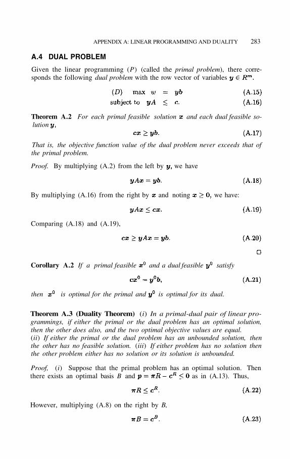
A.4 DUAL PROBLEM

Given the linear programming (P) (called the primal problem), there corre-sponds the following dual problem with the row vector of variables

Theorem A.2 For each primal feasible solution and each dual feasible so-lution

That is, the objective function value of the dual problem never exceeds that ofthe primal problem.

Proof. By multiplying (A.2) from the left by we have

By multiplying (A.16) from the right by and noting we have:

Comparing (A.18) and (A.19),

Corollary A.2 If a primal feasible and a dual feasible satisfy

then is optimal for the primal and is optimal for its dual.

Theorem A.3 (Duality Theorem) (i) In a primal-dual pair of linear pro-grammings, if either the primal or the dual problem has an optimal solution,then the other does also, and the two optimal objective values are equal.(ii) If either the primal or the dual problem has an unbounded solution, thenthe other has no feasible solution. (iii) If either problem has no solution thenthe other problem either has no solution or its solution is unbounded.

Proof, (i) Suppose that the primal problem has an optimal solution. Thenthere exists an optimal basis B and as in (A.13). Thus,

However, multiplying (A.8) on the right by B,


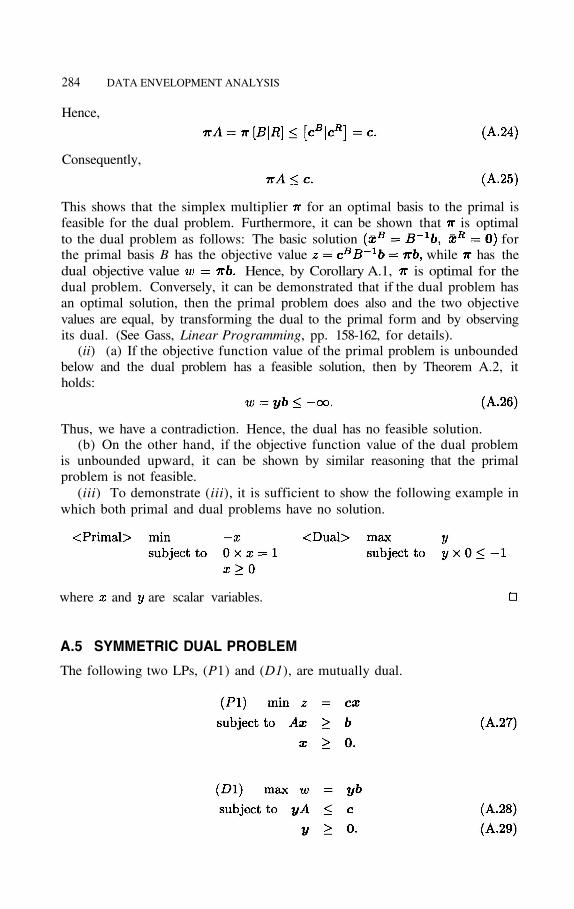
Hence,

Consequently,

This shows that the simplex multiplier for an optimal basis to the primal isfeasible for the dual problem. Furthermore, it can be shown that is optimalto the dual problem as follows: The basic solution forthe primal basis B has the objective value while has thedual objective value Hence, by Corollary A.1, is optimal for thedual problem. Conversely, it can be demonstrated that if the dual problem hasan optimal solution, then the primal problem does also and the two objectivevalues are equal, by transforming the dual to the primal form and by observingits dual. (See Gass, Linear Programming, pp. 158-162, for details).

(ii) (a) If the objective function value of the primal problem is unboundedbelow and the dual problem has a feasible solution, then by Theorem A.2, itholds:

Thus, we have a contradiction. Hence, the dual has no feasible solution.(b) On the other hand, if the objective function value of the dual problem

is unbounded upward, it can be shown by similar reasoning that the primalproblem is not feasible.

(iii) To demonstrate (iii), it is sufficient to show the following example inwhich both primal and dual problems have no solution.

where and are scalar variables.

A.5 SYMMETRIC DUAL PROBLEM

The following two LPs, (P1) and (D1), are mutually dual.


The reason is that, by introducing a nonnegative slack (P1) can berewritten as (P1') below and its dual turns out to be equivalent to (D1) .

This form of mutually dual problems can be depicted as Table A.1, which isexpressed verbally as follows:

For the inequality constraints of the primal (dual) problem, the corre-sponding dual (primal) variables must be nonnegative. The constraints of thedual (primal) problem are bound to inequality The objective functionis to be maximized (minimized).

This pair of LPs are called symmetric primal-dual problems. The dualitytheorem above holds for this pair, too.

A.6 COMPLEMENTARITY THEOREM

Let us transform the symmetric primal-dual problems into equality constraintsby introducing nonnegative slack variables and respectively.

Then, the optimality condition in Duality Theorem A.3 can be stated as follows:

Theorem A.4 (Complementarity Theorem) Let and befeasible to (P1') and (Dl'), respectively. Then, and are optimal


to (P1' ) and (D1' ) if and only if it holds:

Proof.

Thus, By the duality theorem, and are optimal for the primaland the dual, respectively.

By (A.33), we have

By nonnegativity of each term in these two expressions,

Thus, either or must be zero for each and either or must be zerofor each We called this property complementarity.

A.7 FARKAS’ LEMMA AND THEOREM OF THE ALTERNATIVE

Theorem A.5 (Farkas’ Lemma, Theorem of the Alternative) For eachmatrix A and each vector either

has a solution or

has a solution but never both.

Proof. For (I) , we consider the following the primal-dual pair of LPs:


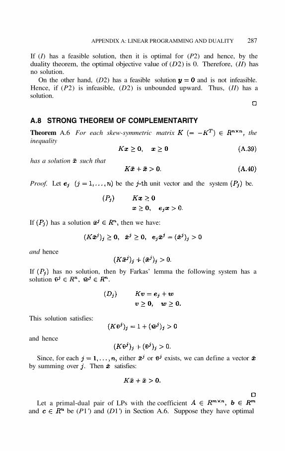
If (I) has a feasible solution, then it is optimal for (P2) and hence, by theduality theorem, the optimal objective value of (D2) is 0. Therefore, (II) hasno solution.

On the other hand, (D2) has a feasible solution and is not infeasible.Hence, if (P2) is infeasible, (D2) is unbounded upward. Thus, (II) has asolution.

A.8 STRONG THEOREM OF COMPLEMENTARITY

Theorem A.6 For each skew-symmetric matrix theinequality

has a solution such that

Proof. Let be the unit vector and the system be.

If has a solution then we have:

and hence

If has no solution, then by Farkas’ lemma the following system has asolution

This solution satisfies:

and hence

Since, for each either or exists, we can define a vectorby summing over Then satisfies:

Let a primal-dual pair of LPs with the coefficientand be (P1') and (D1') in Section A.6. Suppose they have optimal


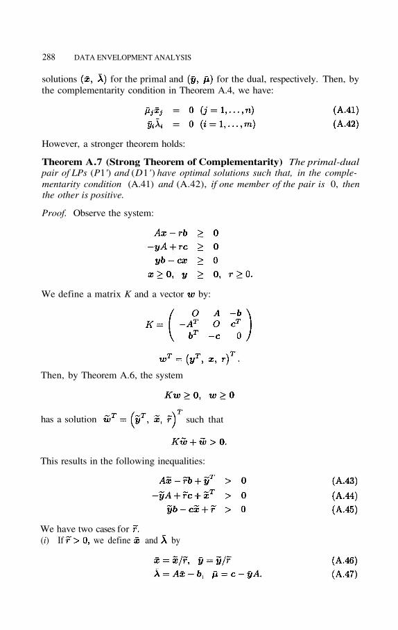
solutions for the primal and for the dual, respectively. Then, bythe complementarity condition in Theorem A.4, we have:

However, a stronger theorem holds:

Theorem A.7 (Strong Theorem of Complementarity) The primal-dualpair of LPs (P1') and (D1 ') have optimal solutions such that, in the comple-mentarity condition (A.41) and (A.42), if one member of the pair is 0, thenthe other is positive.

Proof. Observe the system:

We define a matrix K and a vector by:

Then, by Theorem A.6, the system

has a solution

This results in the following inequalities:

We have two cases for(i) If we define and by

such that


Then, is a feasible solution of (P1') and is a feasible solutionof (D1'). Furthermore, Hence, these solutions are optimal for theprimal-dual pair LPs. In this case, (A.43) and (A.44) result in

Thus, strong complementarity holds as asserted in the theorem.(ii) If it cannot occur that both (P1') and (D1') have feasible solutions.The reason is: if they have feasible solutions and then

Hence, we have:

This contradicts (A.45) in the case Thus, the case cannot occur.

A.9 LINEAR PROGRAMMING AND DUALITY IN GENERAL FORM

As a more general LP, we consider the case when there are both nonnegativevariables and sign-free variables and both inequality andequality constraints are to be satisfied as follows:

where andThe corresponding dual problem is expressed as follows, with variablesand

It can be easily demonstrated that the two problems are mutually primal-dualand the duality theorem holds between them. Table A.2 depicts the generalform of the duality relation of Linear Progrmming.


Now, we introduce slack variables and (DP)and rewrite them as (LP´) and (DP´) below:

We then have the following complementarity theorem:

Corollary A.3 (Complementarity Theorem in General Form)Let and be feasible to (LP') and (DP'), respectively.Then, they are optimal to (LP') and (DP'), if and only if the relation belowholds.

Also, there exist optimal solutions that satisfy the following strong complemen-tarity.


Corollary A.4 (Strong Theorem of Complementarity) In the optimal so-lutions to the primal-dual pair LPs, (LP') and (DP'), there exist ones suchthat, in the complementarity condition (A.56), if one of the pair is 0, then theother is positive.

Notes

l.

2.

3.

4.

5.

6.

7.

S.I. Gass (1985) Linear Programming, 5th ed., McGraw-Hill.

A. Charnes and W.W. Cooper (1961) Management Models and Industrial Applicationsof Linear Programming, (Volume 1 & 2), John Wiley & Sons.

O.L. Mangasarian (1969) Nonlinear Programming, McGraw-Hill.

K. Tone (1978) Mathematical Programming, (in Japanese) Asakura, Tokyo.

G.B. Dantzig (1963) Linear Programming and Extensions (Princeton: Princeton Univer-sity Press).

W.A. Spivey and R.M. Thrall (1970) Linear Optimization (New York: Holt, Rinehartand Winston).

E.D. Nering and A.W. Tucker (1993) Linear Programming and Related Problems (NewYork: Academic Press).


Appendix BIntroduction to DEA-Solver

This is an introduction and manual for the attached DEA-Solver. There are twoversions of DEA-Solver, the “Learning Version” (called DEA-Solver-LV, inthe attached CD) and the “Professional Version” (called DEA-Solver-PRO:visit the DEA-Solver website at: http://www.saitech-inc.com/ for furtherinformation). This manual serves both versions.

B.1 PLATFORM

The platform for this software is Microsoft Excel 97/2000 (a trademark ofMicrosoft Corporation).

B.2 INSTALLATION OF DEA-SOLVER

The accompanying installer will install DEA-Solver and sample problems inthe attached CD to the hard disk (C:) of your PC. Just follow the instructionon the screen. The folder in the hard disk is “C:\DEA-Solver” which includesthe code DEA-Solver.xls and another folder “Samples.” It is recommended thatyou will create the shortcut to DEA-Solver.xls on the display so as to minimizestart-up time. If you want to install “DEA-Solver” to other drive or to otherfolder (not to “C:\DEA-Solver”), just copy it to the disk or to the folder youdesignate. For the “Professional Version” an installer will automatically install“DEA-Solver-PRO.”

B.3 NOTATION OF DEA MODELS

DEA-Solver applies the following notation for describing DEA models.

where I or O corresponds to “Input”- or “Output”-orientation and C or Vto “Constant” or “Variable” returns to scale. For example, “AR-I-C” meansthe Input oriented Assurance Region model under Constant returns-to-scaleassumption. In some cases, “I or 0” and/or “C or V” are omitted. For example,“CCR-I” indicates the Input oriented CCR model which is naturally underconstant returns-to-scale. “Bilateral” and “FDH” have no extensions. Theabbreviated model names correspond to the following models,

1.

2.

3.

4.

5.

CCR = Charnes-Cooper-Rhodes model (Chapters 2, 3)

BCC = Banker-Charnes-Cooper model (Chapters 4, 5)

IRS = Increasing Returns-to-Scale model (Chapter 5)

DRS = Decreasing Returns-to-Scale model (Chapter 5)

GRS = Generalized Returns-to-Scale model (Chapter 5)

<Model Name> - <I or O> - <C or V>

APPENDIX B: DEA-SOLVER 293

6.

7.

8.

9.

10.

11.

12.

13.

14.

15.

16.

17.

18.

AR = Assurance Region model (Chapter 6)

NCN = Uncontrollable (non-discretionary) variable model (Chapter 7)

BND = Bounded variable model (Chapter 7)

CAT = Categorical variable model (Chapter 7)

SYS = Different Systems model (Chapter 7)

SBM = Slacks-Based Measure model (Chapter 4)

Cost = Cost efficiency model (Chapter 8)

Revenue = Revenue efficiency model (Chapter 8)

Profit = Profit efficiency model (Chapter 8)

Ratio = Ratio efficiency model (Chapter 8)

Bilateral = Bilateral comparison model (Chapter 7)

FDH = Free Disposal Hull model (Chapter 4)

Window = Window Analysis (Chapter 9)

B.4 INCLUDED DEA MODELS

The “Learning Version” includes the following 7 models and can solve problemswith up to 50 DMUs;

CCR-I, CCR-O

BCC-I, BCC-O

AR-I-C

NCN-I-C and

Cost-C.

The “Professional Version” includes all 46 models and can deal with large-scaleproblems within the capacity of Excel worksheet. Added to the “LearningVersion” are;

IRS-I, IRS-O

DRS-I, DRS-O

GRS-I, GRS-O

AR-I-V, AR-O-C, AR-O-V

NCN-I-V, NCN-O-C, NCN-O-V

BND-I-C, BND-I-V, BND-O-C, BND-O-V


CAT-I-C, CAT-I-V, CAT-O-C, CAT-O-V

SYS-I-C, SYS-I-V, SYS-O-C, SYS-O-V

SBM-I-C, SBM-I-V, SBM-O-C, SBM-O-V

Cost-V

Revenue-C, Revenue-V

Profit-C, Profit-V

Ratio-C, Ratio-V

Bilateral

FDH and

Window-I-C, Window-I-V.

B.5 PREPARATION OF THE DATA FILE

The data file should be prepared in an Excel Workbook prior to execution ofDEA-Solver. The formats are as follows:

B.5.1 The CCR, BCC, IRS, DRS, GRS, SBM and FDH Models

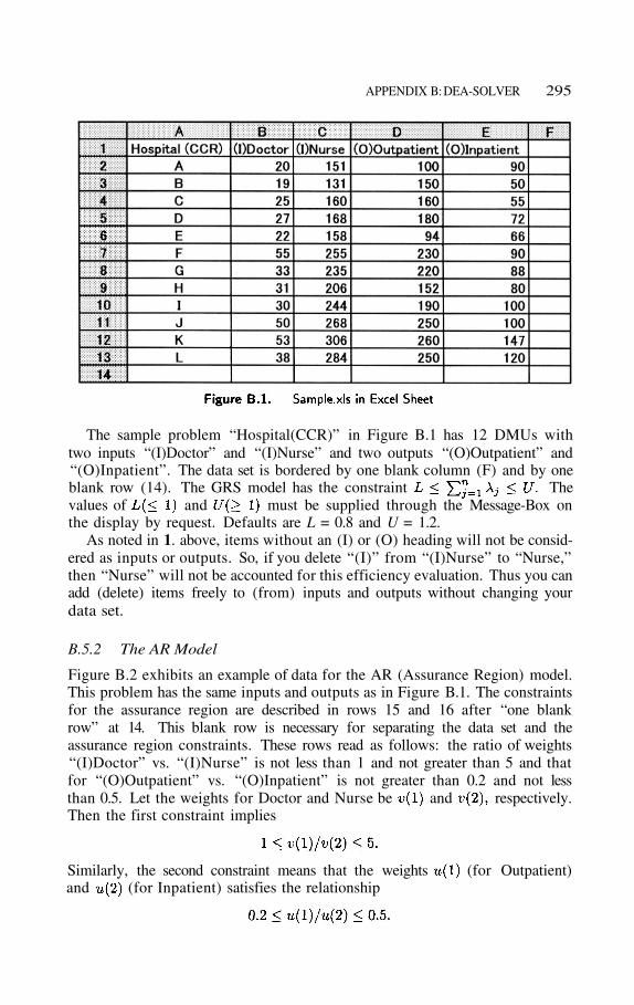
Figure B.1 shows an example of data file for these models.

1. The first row (Row 1)The first row (Row 1) contains Names of Problem and Input/Output Items,i.e.,Cell A1 = Problem NameCell Bl, Cl, . . .= Names of I/O items.The heading (I) or (O), showing them as being input or output should headthe names of I/O items. The items without an (I) or (O) heading will notbe considered as inputs and outputs. The ordering of (I) and (O) items isarbitrary.

2.

3.

4.

The second row and afterThe second row contains the name of the first DMU and I/O values for thecorresponding I/O items. This continues up to the last DMU.The scope of data domainA data set should be bordered by at least one blank column at right and atleast one blank row at bottom. This is a necessity for knowing the scope ofthe data domain. The data set should start from the top-left cell (A1).Data sheet nameA preferable sheet name is “DAT” (not “Sheet 1”). Never use names “Score”,“Rank”, “Projection”, “Weight”, “WeightedData”, “Slack”, “RTS”, “Win-dow”, “Graphl” and “Graph2” for data sheet. These are reserved for thissoftware.


The sample problem “Hospital(CCR)” in Figure B.1 has 12 DMUs withtwo inputs “(I)Doctor” and “(I)Nurse” and two outputs “(O)Outpatient” and“(O)Inpatient”. The data set is bordered by one blank column (F) and by oneblank row (14). The GRS model has the constraint Thevalues of and must be supplied through the Message-Box onthe display by request. Defaults are L = 0.8 and U = 1.2.

As noted in 1. above, items without an (I) or (O) heading will not be consid-ered as inputs or outputs. So, if you delete “(I)” from “(I)Nurse” to “Nurse,”then “Nurse” will not be accounted for this efficiency evaluation. Thus you canadd (delete) items freely to (from) inputs and outputs without changing yourdata set.

B.5.2 The AR Model

Figure B.2 exhibits an example of data for the AR (Assurance Region) model.This problem has the same inputs and outputs as in Figure B.1. The constraintsfor the assurance region are described in rows 15 and 16 after “one blankrow” at 14. This blank row is necessary for separating the data set and theassurance region constraints. These rows read as follows: the ratio of weights“(I)Doctor” vs. “(I)Nurse” is not less than 1 and not greater than 5 and thatfor “(O)Outpatient” vs. “(O)Inpatient” is not greater than 0.2 and not lessthan 0.5. Let the weights for Doctor and Nurse be and respectively.Then the first constraint implies

Similarly, the second constraint means that the weights (for Outpatient)and (for Inpatient) satisfies the relationship


Notice that the weights constraint can be applied within inputs or within out-puts and cannot be applied between inputs and outputs.

B.5.3 The NCN Model

The uncontrollable (non-discretionary) model has basically the same data for-mat as the CCR model. However, the uncontrollable inputs or outputs musthave the headings (IN) or (ON), respectively. Figure B.3 exhibits the casewhere ‘Doctor’ is an uncontrollable (i.e., “non-discretionary” or “exogenouslyfixed”) input and ‘Inpatient’ is an uncontrollable output.


B.5.4 The BND Model

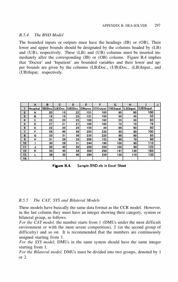
The bounded inputs or outputs must have the headings (IB) or (OB). Theirlower and upper bounds should be designated by the columns headed by (LB)and (UB), respectively. These (LB) and (UB) columns must be inserted im-mediately after the corresponding (IB) or (OB) column. Figure B.4 impliesthat ‘Doctor’ and ‘Inpatient’ are bounded variables and their lower and up-per bounds are given by the columns (LB)Doc., (UB)Doc., (LB)Inpat., and(UB)Inpat, respectively.

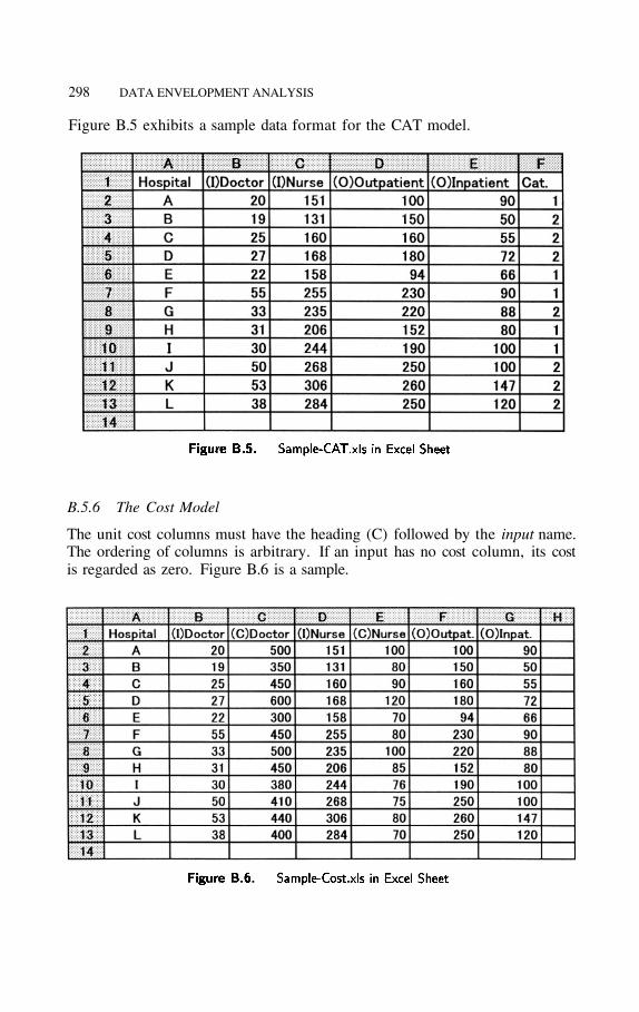
B.5.5 The CAT, SYS and Bilateral Models

These models have basically the same data format as the CCR model. However,in the last column they must have an integer showing their category, system orbilateral group, as follows.For the CAT model, the number starts from 1 (DMUs under the most difficultenvironment or with the most severe competition), 2 (in the second group ofdifficulty) and so on. It is recommended that the numbers are continuouslyassigned starting from 1.For the SYS model, DMUs in the same system should have the same integerstarting from 1.For the Bilateral model, DMUs must be divided into two groups, denoted by 1or 2.


Figure B.5 exhibits a sample data format for the CAT model.

B.5.6 The Cost Model

The unit cost columns must have the heading (C) followed by the input name.The ordering of columns is arbitrary. If an input has no cost column, its costis regarded as zero. Figure B.6 is a sample.


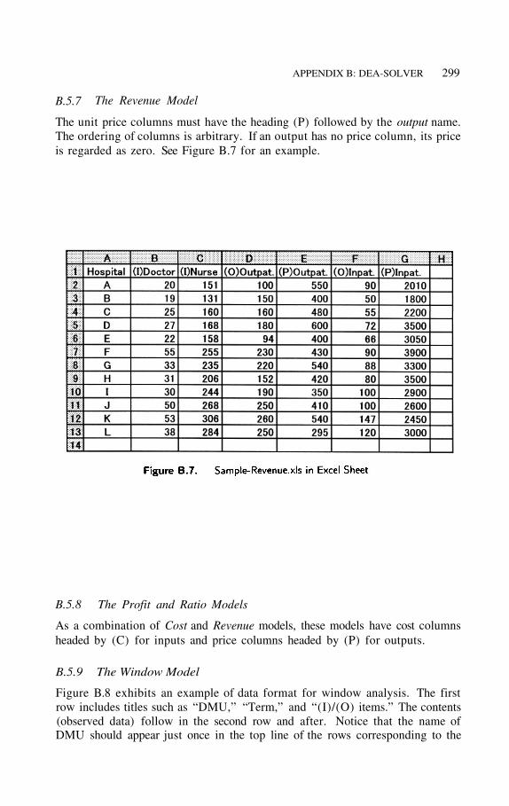
B.5.7 The Revenue Model

The unit price columns must have the heading (P) followed by the output name.The ordering of columns is arbitrary. If an output has no price column, its priceis regarded as zero. See Figure B.7 for an example.

B.5.8 The Profit and Ratio Models

As a combination of Cost and Revenue models, these models have cost columnsheaded by (C) for inputs and price columns headed by (P) for outputs.

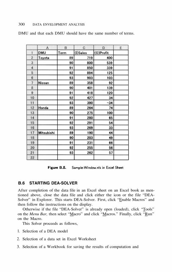
B.5.9 The Window Model

Figure B.8 exhibits an example of data format for window analysis. The firstrow includes titles such as “DMU,” “Term,” and “(I)/(O) items.” The contents(observed data) follow in the second row and after. Notice that the name ofDMU should appear just once in the top line of the rows corresponding to the


DMU and that each DMU should have the same number of terms.

B.6 STARTING DEA-SOLVER

After completion of the data file in an Excel sheet on an Excel book as men-tioned above, close the data file and click either the icon or the file “DEA-Solver” in Explorer. This starts DEA-Solver. First, click “Enable Macros” andthen follow the instructions on the display.

Otherwise if the file “DEA-Solver” is already open (loaded), click “Tools”on the Menu Bar, then select “Macro” and click “Macros.” Finally, click “Run”on the Macro.

This Solver proceeds as follows,

1.

2.

3.

Selection of a DEA model

Selection of a data set in Excel Worksheet

Selection of a Workbook for saving the results of computation and


4. DEA computation

B.7 RESULTS

The results of computation are stored in the selected Excel workbook. Thefollowing worksheets contain the results, although some models lack some ofthem.

1.

2.

Worksheet “Summary”This worksheet shows statistics on data and a summary report of resultsobtained.

Worksheet “Score”This worksheet contains the DEA-score, reference set, for each DMUin the reference set and ranking in input and in the descending order ofefficiency scores. A part of a sample Worksheet “Score” is displayed inFigure B.9, where it is shown that DMUs A, B and D are efficient (Score=l)and DMU C is inefficient (Score=0.882708) with the reference set composedof and and so on.

In the “Professional Version,” the ranking of DMUs in the descending orderof efficiency scores will be listed in the worksheet “Rank”.

3.

4.

Worksheet “Projection”This worksheet contains projections of each DMU onto the efficient frontierby the chosen model.

Worksheet “Weight”Optimal weights and for inputs and outputs are exhibited in this


worksheet. corresponds to the constraints and toIn the BCC model where holds, stands for

the value of the dual variable for this constraint.

5.

6.

7.

Worksheet “WeightedData”This worksheet shows the optimal weighted I/O values, andfor each (for

Worksheet “Slack”This worksheet contains the input excesses and output shortfalls foreach DMU.

Worksheet “RTS”In case of the BCC, AR-I-V and AR-O-V models, the returns-to-scale char-acteristics are recorded in this worksheet. For inefficient DMUs, returns-to-scale characteristics are those of the (input- or output-oriented) projectedDMUs on the frontier.

8.

9.

Graphsheet “Graph1”The bar chart of the DEA scores is exhibited in this graphsheet. This graphcan be redesigned using the Graph functions of Excel.

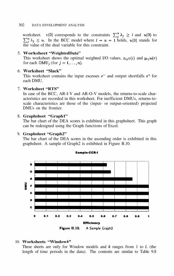
Graphsheet “Graph2”The bar chart of the DEA scores in the ascending order is exhibited in thisgraphsheet. A sample of Graph2 is exhibited in Figure B.10.

10. Worksheets “WindowThese sheets are only for Window models and ranges from 1 to L (thelength of time periods in the data). The contents are similar to Table 9.8


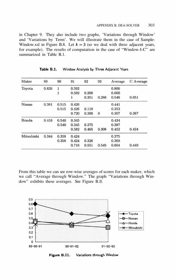
in Chapter 9. They also include two graphs, ‘Variations through Window’and ‘Variations by Term’. We will illustrate them in the case of Sample-Window.xsl in Figure B.8. Let (so we deal with three adjacent years,for example). The results of computation in the case of “Window-I-C” aresummarized in Table B.1.

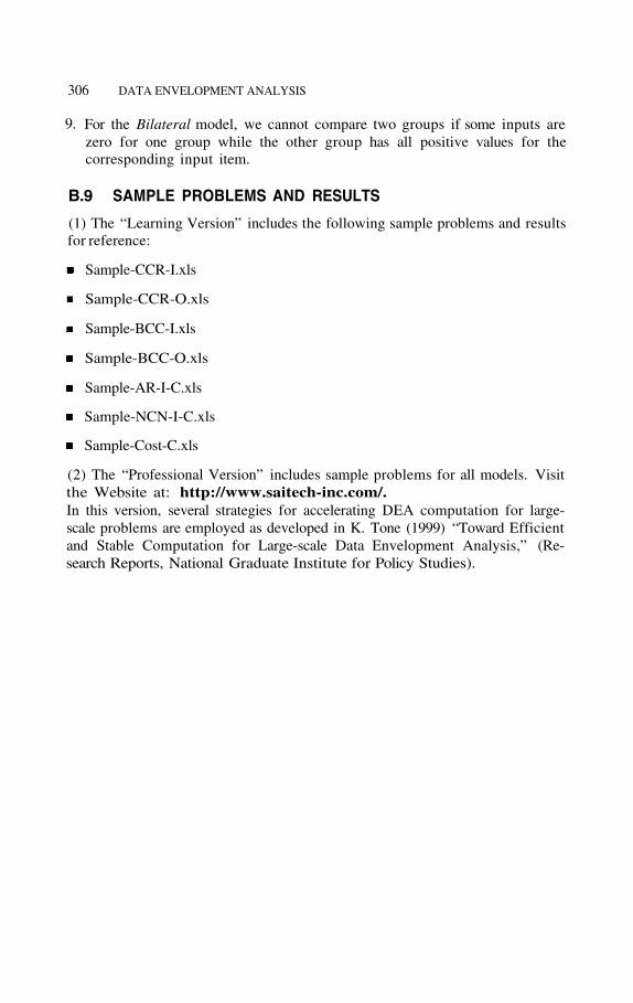
From this table we can see row-wise averages of scores for each maker, whichwe call “Average through Window.” The graph “Variations through Win-dow” exhibits these averages. See Figure B.ll.


We can also evaluate column-wise averages of scores for each maker, whichwe call “Average by Term.” The graph “Variations by Term” exhibits theseaverages. See Figure B.12.

Note. The BCC, AR-I-V and AR-O-V models contain all the worksheets ex-cept “Window.” The CCR, IRS, DRS, GRS, AR-I-C, AR-O-C and SBM modelscontain all sheets except “RTS” and “Window.” The NCN, BND, CAT, SYS,Cost, Revenue, Profit, Ratio and FDH models produce “Summary,” (“Rank,”)“Score,” “Projection,” “Graphl” and “Graph2.” The Bilateral model shows“Summary,” “Score” and “Rank” sheets. The Window model contains only“Window” sheets.

B.8 DATA LIMITATIONS

B.8.1 Problem Size

The “Learning Version” in the attached CD can solve problems with up to 50DMUs. In the “Professional Version,” the problem size is unlimited in terms ofthe number of DMUs and I/O items within the capacity of an Excel worksheetand the main memory of PC. More concretely, the data limitations for the“Professional Version” are as follows;

1.

2.

No. of DMUs must be less than 60000.

If No. of then the“Projection” sheet will not be provided.

B.8.2 Inappropriate Data for Each Model

DMUs with the following irregular data are excluded from the comparison groupas “inappropriate” DMUs. They are listed in the Worksheet “Summary.” Wewill adopt the following notations for this purpose.

= the max (min) input value of the DMU concerned


= the max (min) output value of the DMU concerned

= the max (min) unit cost of the DMU concerned

= the max (min) unit price of the DMU concerned

1. For the CCR, BCC-I, IRS, DRS, GRS, CAT and SYS models, a DMUwith no positive value in inputs, i.e., will be excluded fromcomputation. Zero or minus values are permitted if there is at least onepositive value in the inputs of the DMU concerned.

For the BCC-O model, DMUs with no positive value in outputs, i.e.,will be excluded from computation.

2. For the AR model, i.e., AR-I-C, AR-I-V, AR-O-C and AR-O- V, DMUs with or will be excluded from the comparison

group.

3.

4.

5.

For the FDH model, DMUs with no positive input value, i.e., ora negative input value, i.e., will be excluded from computation.

For the Cost model, DMUs with or are excluded. DMUs with the current input will also

be excluded.

For the Revenue, Profit and Ratio models, DMUs with no positive inputvalue, i.e., no positive output value, i.e., or witha negative output value, i.e., will be excluded from computa-tion. Furthermore, in the Revenue model, DMUs with or

will be excluded from the comparison group. In the Profitmodel DMUs with or will be excluded. Finally,in the Ratio model, DMUs with ,or will be excluded.

6. For the NCN and BND models, negative input and output values are auto-matically set to zero by the program. DMUs with in the control-lable (discretionary) input variables will be excluded from the comparisongroup as “inappropriate” DMUs. In the BND model, the lower bound andthe upper bound must enclose the given (observed) value, otherwise thesevalues will be adjusted to the given value.

7. For the Window-I-C and Window-I-V models, no restriction exists for outputdata, i.e., positive, zero or negative values for outputs are permitted. How-ever, DMUs with will be characterized as being zero efficiency.This is for purpose of completing the score matrix. So, care is needed forinterpreting the results in this case.

8. For the SBM model, nonpositive inputs or outputs are replaced by a smallpositive value.


9. For the Bilateral model, we cannot compare two groups if some inputs arezero for one group while the other group has all positive values for thecorresponding input item.

B.9 SAMPLE PROBLEMS AND RESULTS

(1) The “Learning Version” includes the following sample problems and resultsfor reference:

Sample-CCR-I.xls

Sample-CCR-O.xls

Sample-BCC-I.xls

Sample-BCC-O.xls

Sample-AR-I-C.xls

Sample-NCN-I-C.xls

Sample-Cost-C.xls

(2) The “Professional Version” includes sample problems for all models. Visitthe Website at: http://www.saitech-inc.com/.In this version, several strategies for accelerating DEA computation for large-scale problems are employed as developed in K. Tone (1999) “Toward Efficientand Stable Computation for Large-scale Data Envelopment Analysis,” (Re-search Reports, National Graduate Institute for Policy Studies).

APPENDIX C: BIBLIOGRAPHY 307

Appendix CBibliography

Comprehensive bibliography of 1500 DEA references is available in the attachedCD-ROM.

Author Index

Adolphson, 205Ahn, 92, 112, 127Aigner, 259Ali, xxiv, 73, 96, 104, 109, 112Andersen, 278Arnold, 66, 74, 261Aronson, 74Athanassopoulos, 174, 181, 249Banker, 63, 85, 88, 104, 121–122, 126, 128,

183, 205Bardhan, 66, 74, 121, 262Barr, 181Battese, 265Baumol, 247Bowlin, 106, 113Brennan,113Brockett, xx, xxiv, 163, 174, 181, 204, 206,

219, 251Bulla, 36Chang, 122Charnes, xxi, 19, 21, 46, 69, 85, 88, 104,

113, 151, 184, 205–206, 252, 268, 281Chu, 259Coelli, 61, 265Cook, xxiv, 152Cooper, xxi, xxiv, 19–21, 36, 46, 69, 85, 88,

104, 113, 121–122, 151, 206, 222, 225,251–252, 255, 266, 268, 277, 281

Cummins, xxDantzig, 281Debreu, 69, 223Deprins, 105, 113Desai, 174, 182Dharmapala, 35, 278Diaz, 77Divine, 108Dyson, 174, 181, 249Fama, xx, 204Farkas, 286Farrell, 33, 44–45, 69, 72, 223, 259, 279

Ferrier, 260Fried, 73Frisch, 150Färe, 73, 113, 147, 221, 242, 272, 280Førsund, 150Gallegos, 74Gass, 281, 284Golany, xx, 152, 174, 206Gong, 260Gonzalez-Lima, 77Greville, 181Grosskopf, 73, 147, 221, 242, 272, 280Gu, 252Haag, 278Haynes, 174, 182Hoffman, 69Huang, 151, 174, 266, 269–271, 279Ijiri, 20Jaska, 278Jensen, xx, 204Jondrow, 260Joro, xxivKamakura, 206Klopp, 272Koopmans, xxii, 45, 68, 73Korhonen, xxivKorostolev, 259Kozmetsky, 233Kumbhakar, 265, 279Land, 267Langemeir, 174Lee, 174Lehman, 219Lelas, 271Lewin, xxi, 77, 83, 251, 277–278Li, 252, 255, 266, 269–270, 279Lovell, 67, 73, 113, 147, 221, 242, 259–260,

265, 267, 279Maindiratta, 111Mangasarian, 281


Mann, 200Markowitz, 269Materov, 260Morey, 63, 77, 126, 183, 205, 277Neralic, 77, 252, 278Nering, 281Nun, 164Olesen, 271, 280Panzar, 247Pareto, xxii, 45, 68Park, xxiv, 36, 222, 225Pastor, 104, 109, 222, 225Petersen, 271, 278, 280Phillips, 233Rao, 265Rhodes, 19, 21, 46, 69, 206Roll, 152, 174Rousseau, 77, 206, 277–278Ruefli, 108Russell, 113Saaty, 170Schmidt, 73, 259Seiford, xxi, xxiv, 73, 83, 96, 104, 109,

111–112, 150, 181–182, 251, 255,277–278

Semple, 206, 278Sengupta, 272, 280Sharpe, 269Sherman, 18, 20Shin, 251Sickles, 260Siems, 181Simar, 105, 113, 278Simon, xxv, 266, 279

Singleton, 151Smith, 151Spivey, 281Storbeck, 174, 181Stutz, 111Sueyoshi, 113, 261, 273Sun, 151, 174, 275Thanassoulis, 174, 181, 249Thomas, 107Thompson, 35, 77, 151, 255Thore, 233, 266–267Thrall, 35, 77, 104, 106, 109, 121–122, 151,

255, 281Tone, 83, 101, 104, 113, 131, 144, 169, 175,

181, 205–206, 249, 252, 255, 281, 306Triantis, xxivTsybakov, 278Tucker, 281Tulkens, 105, 113Varian, 20Wallenius, xxivWalters, 83Wang, 251Wei, xxiv, 174Wein, 130, 246Whitney, 200Wilcoxon, 200Wfflig, 247Wilson, 36, 252, 277, 279Wood, 83Yu, xxivZhu, 150, 251, 255, 277–278Zi, xxZionts, 74

Topic Index

A prioriassumptions, 13choices of weights, 13determination, 15knowledge, 151

Absolute bounds, 152Academic performance, 66Activity analysis, 68Activity, 42ADD-efficient, 92Additive model, 85–86, 91, 184, 222, 225,

231non-discretionary variables, 184vs BCC model, 93

Admissibledirections, 162directions

selecting, 162nonnegative direction vectors, 159

Advantages of DEA, 14Agency theory, xx, 204Allocative

efficiency, 221, 223–225, 231, 235, 242efficiency

generalization of, 152inefficiency, xxiii, 94, 225, 231model, 94

Alternate optima, 231Analytic Hierarchy Process, 170, 251AR

assurance region, 152, 175efficiency, 153

AR-efficiency, 153Archimedean property, 74Army recruiting, xxiv, 272Assurance region, 151–152, 164, 174, 185

as special case of cone-ratio, 160constraints, 157, 172, 179method, 152vs cone-ratio, 159

Average behavior, 4Average productivity, 115Balance sheet, 164Bank

failures, 163management incompetence, 165merger, 143

simulation, 139performance, 151

Banker-Morey model, 212Banks, xx

Japan,140Texas, 163

Baseball teams, 190, 217Basel Agreement, 163Basic Additive model, 91Basic solution, 281–282Basis, 281–282Batting average, 191BCC

Banker, Charnes, Cooper model, 85efficiency, 89envelopment form, 90fractional program, 88, 91model, 85, 87

vs Additive model, 93multiplier form, 88, 90production possibility set, 88reference set, 89returns-to-scale, 120two-phase procedure, 89

BCC-efficient, 87, 89BCC-I, 106, 146BCC-inefficient, 89BCC-O, 106, 146BCC-projection, 90Benchmark, 4Benchmarking, 2Best performance, 4Best ratio, 13

312

Best set of weights, 13Bilateral comparisons, 201–202, 206, 217

example, 203model, 207

BND, 206Bootstrap method, 259Bounded variable model, 190Bounded

non-discretionary variable, 190projection, 192variable, 192

model, 190, 206Bounds

absolute, 152lower and upper, 158on multipliers, 158on slacks, 226on specific variables, 164

Branch banks, xixBranch office example, 8Branch store, 193

example, 3Canada, xixCandidate reference point, 195Candidate sites, 169, 173CAT, 206Categorical

(classificatory) variable, 184level, 193

algorithm, 195levels expanded, 215model, 194variable, xxiv, 184, 205

Categories, 215CCP, 266, 271CCR

Charnes, Cooper, Rhodes model, 21dual problem, 41model, 13, 21projection, 47, 49, 188returns-to-scale, 122two-phase procedure, 46weak efficiency form, 100

CCR-AR model, 153CCR-efficiency, 24, 46, 101CCR-efficient, 68, 87CCR-I, 70CCR-inefficiency, 24CCR-O, 70CCR-type models, 86Central tendency behavior, 4Chain-store example, 19Chance-constrained programming, xxv, 266,

276Charnes-Cooper transformation, 72, 234Charnes-Cooper-Rousseau-Semple model,

212

Chebychev norm, 253, 255Cities, xixClassificatory variable, xxiv, 184Cobb-Douglas, 103, 110, 260

envelopment, 111form, 261regression, 261

Column views, 273Combustion engineering, 6Commercial banks, 174Comparing

DEA scores of two groups, 201efficient frontiers of two groups, 201

Comparisonsof different systems, 197of efficiencies, 200of efficiency, 207

Complementarity theorem, 285Complementary condition, 46Complementary slackness, xxii, 83, 158

and sensitivity analysis, 78Composed error, 259Computational aspects of DEA, 50Computational procedures, 50Conditional chance constraints, 271Cone-ratio, 151

as generalization of assurance region, 160envelopment, 151, 164, 185example, 161method, 159, 174

formula, 160vs assurance region, 159

Confidence intervals, 259Congestion, 251Consensus formation, 169Consensus, 170Consensus-making, 169, 171Consistent estimator, 259Constant returns-to-scale, 85, 117, 122

assumption, 4, 42, 68, 85Contestable markets, 247Controllable

categorical level, 195variable, 187

Convexcone, 159hull, 85, 104

Convexityassumption, 197condition, 88, 109, 134

Costefficiency, 236minimization, 238

Cost-C(V), 236Countries, xixCRS, 132Cyprus, xix

313

DRS, 132DRS-I, 146DRS-O, 146DSI-Athens meeting, xxiDual feasible solution, 283Dual problem, 43, 283Dual simplex, 52Dual theorem of linear programming, 177Duality, 281

relations, xxiitheorem, 35, 283, 285

Dummy variables, xxiv, 261Economic efficiency, 11Economics, xxiEconomies of scope, 251Economists, xxiEffectiveness, 66

vs efficiency, 164Effects of a merger, 143Efficiency, 3, 66

audits, 107dominance, 271prices, 69variance, 11vs effectiveness, 164

Efficient frontier, 3, 25, 87, 92, 123Elasticity, 117, 129

of scale, 117Electric power industries, 200England, xixEnvelop, 3Enveloped, 52Envelopment

form, xxii, 52, 90map, 37model, 68

Equal sample size, 219Euclidean

measure, 10metric, 242

Evaluation by experts, 164Evaluator, 173Excel data sheet, xxiiExogenously fixed, 63

inputs and outputs, 205Expert evaluations, 164Extended additive model, 186Extreme efficient point, 257Facet, 123Farrell efficiency, 44, 46Farrell-Debreu measure, 240–241Fast-food outlets, xxivFast-food restaurants, 63FDH, 105, 107, 219

mixed integer program, 106model, 87

Feasible solution, 281

Data Envelopment Analysis, 2, 33, 52Data

imprecise, xxviiinappropriate, 304limitation, 304variability, 276variations, 251

DEA likelihood estimator, 259DEA web sites, xxiDEA, 2DEA-Solver, xxii, 17, 42, 53, 70, 106, 146,

175, 206, 214, 236, 247, 277, 292AR model, 295Bilateral model, 297BND model, 297CAT model, 297Cost model, 298data file, 294inappropriate data, 304installation, 292learning version, 292-293limitations, 304manual, 292model notation, 292NCN model, 296professional version, xxiii, 292–293Profit model, 299Ratio model, 299results, 301Revenue model, 299sample problems, 306starting, 300SYS model, 297website, 292Window model, 299worksheets, 301

DEA-Solver-LV, 292DEA-Solver-PRO, 292Decision Making Unit, xx, 22, 33Decision Sciences Institute, xxiDecomposition

of efficiency, 137of technical efficiency, 136, 139

Decreasing returns-to-scale, 85, 117, 135Definition of SBM, 97Degrees of discretion, 184Degrees of freedom, 252Demutualizations, xxDepartment stores, 200Deteriorating behavior, 273Deterministic, 266Diet of Japan, 169Different organization forms, 204Dimension free, 97Discretionary variable, 63, 184, 272Distance measure, 9DMU, 22, 33

FGL measure of overall efficiency, 242Fighter Command of U.S. Air Force, 63Financial institutions, 139Fixed weights, 12, 14

vs. variable weights, 12Formula for cone-ratio method, 160Fractional programming, 72, 234

formulation for BCC, 91problem, 23, 249program, 24

France, xixFree disposal hull

example, 105model, 87, 105

Free disposal, 73Free slacks, 227Full efficiency, 233Functional efficiency, 69Furnace efficiency, 6Fuzzy sets, xxiv, 251Gauge of scale efficiency, 126General hospital

case, 161example, 155

Generalization of allocative and priceefficiency, 152

Generalized inverse, 181Generalized returns-to-scale, 135Global technical efficiency, 136Group decision making, 170Group decision problem, 172Groups of DMUs, 201GRS, 135GRS-I, 146GRS-O, 146Halfepaces, 119Hierarchical category, 193

model, 206High-energy physics laboratory, 151Home runs, 191Hospital example, 12, 149Hyperplane, 34, 119Imprecise Data, xxviiImputed (shadow) price, 158Inappropriate data, 304Income statement, 164Inconsistent constraints, 266Incorporating judgement, 151Increasing returns-to-scale, 85, 117, 134Input

data matrix, 22excess, 44mix inefficiency, 98numeraire, 152reduction, 93weights, 23

Input-oriented, 103

assurance region model, 175BCC model, 88CCR model, 41, 58measure of mix inefficiency, 98SBM, 111

model, 138Insurance, 167

companies, xixindustry, 204

Inter-group comparison, 201Interior point algorithm, 259IRS, 132IRS-I, 146IRS-O, 146Isoquant, 223Issues of substitution, 225Japanese banks, 140Japanese capital, 169Japanese Financial Supervisory Agency, 143Jet Engines, 36Joint chance constraints, 271Joint constraints, 271Judgement, 173K-Efficiency, 69Kinds of efficiency, xxiiiLearning version of DEA-Solver, 292Levels of service, 195Library problem, 203Linear program, 23Linear programming, xxii, 281

problem, 281Linkage constraints, 178Linked cone, 178Linked constraint, 174Linked-cone DEA, 178Local pure technical efficiency, 136Log-linear, 260Lost profit opportunity, 233Lower and upper bounds, 158Maintenance activities, xixManagement Science, xxiManagement scientists, xxiManagerial

efficiency, 70performance, 164

Mann-Whitney statistic, 219Marginal productivity, 115Massachusetts, 18, xxiMax-slack solution, 45, 47, 49Maximizing profit, 234Maximizing revenue/expenses ratio, 234Maximum capacity, 190Maximum profitability, 233MCDM, xxivMDI (Minimum Discrimination

Information) Statistic, xxMerger

314

effect, 143Methodological bias, 261Minimal cost, 224Mix

changes, 246efficiency, 138inefficiencies, xxiii, 45inefficiency, 10, 225

Model selection, 102issue of, 87

Monotone, 97Most favorable weights, 25Most productive scale size, 126, 128, 136

MPSS, 126Moving averages, xxvMPSS, 126, 128, 130, 145

fractional program, 128Multicriteria decision-making, xxivMultiple interacting objectives, 204Multiple objective

optimization, 251programming, xxiv

Multiple optimal solutions, 99Multiple reference sets, 83Multiplicative efficiency, 111Multiplicative model, 87, 110, 219Multiplier

bounds, 152form, xxii, 52, 88, 90model approach, 255model, 35, 68, 256space, 30, 34

Mutual companies, 204Mutual funds, xxNCN, 188, 206NCN-projection, 189NDRS, 134Negative slack values, 167New capital for Japan, 169New capital, 169New insights, xixNIRS, 135Non-Archimedean

condition, 75element, 74, 122, 256infinitesimal, 74

Non-controllable variable, 187-188model, 206

Non-decreasing returns-to-scale, 134Non-discretionary, xxiii, 205

extensions, 190inputs and outputs, 190variable, 63, 183, 207, 212, 272

Non-increasing returns-to-scale, 135Nonconvex (staircase) production possibility

set, 87Nonnegativity constraint, 23, 169

Nonnegativity requirements, 168Nonparametric statistics, 200Nonparametric tests, 200Nonunique reference set, 99Nonzero slack, 184Normalization condition, 119Null hypothesis, 201Number of DMUs, 103, 275Numeraire, 152Odense University, xxiOLS, 261Operations Research, xxiOperations researchers, xxiOpportunity cost, 222Optimal

simplex tableau, 51solution, 231, 281weights, 25

Ordinal relations, xxivOrdinary least squares, 261Organization forms, xixOutput

data matrix, 22expansion, 93mix inefficiency, 98multiplier bounds, 159numeraire, 152shortfall, 44weights, 23

Output-input ratio, 1Output-oriented, 103

assurance region model, 155, 175BCC model, 90CCR model, 41, 59model, 58scale efficiency, 138

Output-to-input ratio, 1Overall

efficiency, 224, 235, 242inefficiency, 225

Parallel translation of the coordinatesystem, 86

Pareto-Koopmans efficiency, xxii, 45–46PARN, xxiPartial productivity measure, 1Peer (comparison) group, xxPeer group, 25Peer set, 60Phase II extension, 44Phase II objective, 51Phase III, 60Physical variance, 11Piecewise linear function, 118Point-to-hyperplane correspondence, 34Points at infinity, 46Police forces, xixPolyhedral convex cone, 159

315

Portfolio analysis, 269Positive data set assumption, 41Positive threshold input value, 118Positivity assumptions, 14Price

efficiency, 224efficiency

generalization of, 152inefficiencies, 94

Pricing vector, 52Primal

feasible solution, 283problem, 283

Primal-dual correspondences, 43, 89Principal components analysis, 191Probabilistic formulation, 251, 276Product of Input and Output Inefficiencies,

viii, 98Production economics, xxiiProduction function, 115, 260Production possibility set, 7, 41–42, 68,

87-88, 92, 104, 115, 119, 197, 223Productivity Analysis Research Network

(PARN), xxiProductivity, 1, 3Professional version of DEA-Solver, xxiii,

292–293Profit efficiency, 234, 237Profit maximization, 238, 246Profit ratio, 233Profit-C(V), 237Profit-maximization mix, 234Program efficiency, 70Program Follow Through, 69

experiment, 33Projection

Additive model, 92BCC, 90CCR, 47MPSS, 126bounded, 192NCN, 189SBM, 99

Proportional change, 129Public interest, 204Public libraries, 188, 193Public programs, 235Public schools, 261Public vs private universities, 112Pure technial efficiency, 137Purely technical inefficiency, 11, 94, 98Quality-of-life, xixRadial

(proportional) efficiency, 86efficiency, 45, 86measure, 9, 11

Radius of stability, 254

RAM, 228Range adjusted measure of efficiency, 228Range Adjusted Measure, 228Rank order statistic, xxRank-sum-test, 200Ratio (revenue/cost) efficiency, 237Ratio efficiency, 247Ratio form of DEA, 70Ratio form, 1Ratio of ratios, 35Ratio-C(V), 237Reciprocal relation, 88Reference set, 7, 25, 47, 99Refusal to play, 271Regions, xixRegression analysis vs DEA, 4Regression line, 4Regression with dummy variable values, 263Regression, xxivRegulated Electric Cooperatives, 108Relative efficiency, 5Restricted problem, 51Restricted tableau, 51Returns to scale, 115, 145, 246Returns-to-scale

BCC characterization, 120–121CCR characterization, 122characterization, 120constant, 85decreasing, 85efficiency, 125evaluation, 147generalized, 135identifying, 132–133increasing, 85inefficiencies, xxiiinon-decreasing, 134non-increasing, 135reference set characterization, 132variable, 85

Revenue maximization, 236Revenue vs. cost ratio, 234Revenue-C(V), 236Risk adjusted capital, 163Risk coverage, 164Robustness, 252Round robin procedure, 273Row views, 273Russell input measure, 112Sales environment, 193Sample size, 219Satisficing, xxv, 266

behavior, 266SBM, 97, 107, 138, 273

definition of, 97SBM-efficiency, 101SBM-efficient, 99

316

SBM-inefficient DMU, 99SBM-projection, 99Scale efficiency, 126, 136Scale inefficiency, 93, 148Schools

Texas, 183SCSC, 259Second stage optimization, 94Security banks, xxSemipositive, 42, 150

data, 41Semipositivity, 67Sensitivity analysis, xxv, 251–252, 255Sensitivity, xxv, 112, 252, 276Separate efficiency frontiers, xxSF, 261Shape of the Production Possibility Set, 102Sharper discrimination among DMUs, 104Shortage of outpatients, 155Simple ratio definition, xxiiSimplex

criterion, 282method, 52, 282multiplier, 52, 282

Simulation experiment, 261Single-output-to-single-input ratio, 2Site

evaluation, 170selection, 151, 174

Sites for new capital of Japan, 169Slack vectors, 44Slacks, 168Slacks-based measure of efficiency, 86, 96,

104, 138Solvency, 219Splitting variables, 268Stability, xxv, 252

analysis, 276Staircase (or step) function, 105Standard normal distribution, 201State-mandated Excellence Standards for

Texas, 66Statistical

approach, 259characterizations, 251issues, 200methods, 259regression model, 259regression, 272, 276tests of significance, 259

Status quo, 8Steady behavior, 273Steel industry, 246Stochastic frontier

regression, xxviiStochastic

characterizations, 251

efficiency, 270–271frontier, 247, 261

regression, 259Stock companies, 204Stock vs. mutual, xxStrong complementarity theorem, 46Strong Complementary Slackness Condition,

259Strong disposal, 72Strong theorem of complementarity, 287, 46Subjective judgement, 170Summary

of model characteristics, 102of the Basic DEA Models, 101

Supercolliding Super Conductor, 174Supermarket, 193, 200

example, 6, 215Supporting hyperplane, 119

as dual solution, 120nonunique, 120

Surgical units, 18Surplus in doctors, 155Symmetric primal-dual problems, 285SYS, 207Target entity, 13TDT measure, 35Teaching hospitals, 18Team power, 191Technical

efficiency, 11, 45, 94, 137, 224inefficiency, xxiii, 10, 93, 225vs mix inefficiency, 94

Texas Assessment of Academic Skills(TAAS) Test, 66

Texas Banking Commission, 163Texas banks, 163Texas Education Agency, 65Texas Public Utility Commission, 107Texas schools, 183Texas State Auditor’s Office, 167Theorem of the alternative, 286Time series, 272Time-dependent, 272Total factor productivity, 1, 14Total profit foregone, 227Transformed data, 167Translation invariance, 94, 103–104, 228Trends, 276Two-phase LP problem, 44Two-phase procedure, 74, 89Two-stage analysis, xxTwo-stage DEA-regression approach, 261Two-stage process

DEA and regression, xxivTwo-stage solution procedure, 122U.S. Army Recruiting Command, 272Unequal sample size, 219

317

Unit ball, 254Unit cost, 158United States, xixUnitized axes, 6Units invariance, 6, 15

theorem, 24Units invariant, 6, 24, 61, 97, 111, 228Universities, xix

public vs. private, 112University of Massachusetts–Amherst, xxiUniversity of Warwick, xxiUnstable point, 255USAREC, 272Variable returns-to-scale, 85Variable weights, 13–14

vs. fixed weights, 12Vector of multipliers, 51Virtual input, 21, 23, 33Virtual output, 21, 23, 33Visual Basic, xxiiWales, xixWarwick, xxi

Waste, 11Weak and strong disposal assumptions, 73Weak disposal, 72Weak efficiency, 45–46, 72, 86, 94

form for CCR model, 100Weather conditions, xxivWeb site

UMass, xxiWarwick, xxi

Web sites for DEA, xxiWebsite for DEA-Solver, 292Welfare economics, xxii, 68Welfare efficiency, xxiiWilcoxon-Mann-Whitney, x, 200

statistic, 205Window analysis, xxv, 251–252, 272, 276

column views, 273row views, 273

Window-I-C(V), 277Wise men, 169Within group comparison, 201Zero order decision rules, 271

318

Appendix A Linear Programming and Duality - Springer978-0-306-47541-2/1.pdf · Appendix A Linear...

Documents

Transcript of Appendix A Linear Programming and Duality - Springer978-0-306-47541-2/1.pdf · Appendix A Linear...