Appendix A Environmental Lead and Exposure Trends · PDF file · 2006-06-21A - 1...

Appendix A

Environmental Lead and Exposure Trends

A - 1

Appendix A

Environmental Lead and Exposure Trends

Environmental Lead Trends

Over the past several years, exposure to lead from environmental media (food, water, andair) has declined, and average blood lead levels in the population have declined as well. Today, at most air monitoring sites in California, concentrations of lead in the ambient air are farless than the State Ambient Air Quality Standard of 1.5 µg/m3 over a 30-day averaging time. Atcriteria pollutant monitoring network sites (State/Local Air Monitoring Stations (SLAMS) orNational Air Monitoring Stations (NAMS) which are intended to represent population exposure),the highest monthly means have dropped from 0.29 µg/m3 in 1991 to 0.08 µg/m3 in 1997. Figure A-1 shows the monthly mean lead concentration at the highest criteria pollutant monitoringsite in the State from 1991 to 1997. The site with the highest monthly mean would notnecessarily be the same site from year to year.

Figure A-1: Statewide Maximum Monthly Mean Lead Concentrations

Air Concentration (µg/m3)Monthly Mean

Year

A - 2

Another way to characterize the ambient concentration decreases is to look at the numberof times per year that the monthly mean exceeded 0.10 µg/m3 at SLAMS/NAMS stations. This issummarized in Table A-1.

Table A-1Number of Site-Months with Lead Concentrations1 $$ 0.10 µg/m3

Year Number at or over 0.10 µg/m3

1991 19

1992 7

1993 3

1994 3

1995 0

1996 0

1997 0

1 at SLAMS/NAMS sites

Some special purpose monitors located near large sources or locations potentially affectedby historic emissions have detected higher concentrations. Monthly mean concen-trations up to1.83 µg/m3 at one site in 1993 and 3.98 µg/m3 at another in 1994 have been measured. Thesevalues are believed to be the result of unusual events or conditions.

The statewide population-weighted annual mean concentrations of lead in the ambient airhave dropped precipitously over the last 20 years. Figure A-2 shows the reduction in thestatewide population-weighted annual mean air lead concentrations for the years 1990 to 1997.

Annual mean lead levels higher than the surrounding urban background concentrations of0.01 to 0.03 µg/m3 have been measured in industrial areas which are near large lead processingfacilities and major freeways. These higher than average levels have occurred despite the currentuse of highly effective lead emission controls on the facilities. The sources and district continue tomonitor and address the cause(s) of the air lead levels above background.

Blood Lead Level Trends

The U. S. Department of Health and Human Services, Centers for Disease Control andPrevention (CDC) has investigated the distribution of blood lead levels (BLLs) in the UnitedStates population using large cross-sectional national surveys. These studies have showndecreasing BLLs over the last two decades.

A - 3

Figure A-2: Statewide Population-Weighted Annual Mean Lead Levels

The second National Health and Nutritional Examination Survey (NHANES) II wasconducted from 1976 to 1980. The population was surveyed again from 1988 to 1991 forNHANES III, phase 1 and from 1991 to 1994 for phase 2. These large-scale studies havedocumented an overall decrease in blood lead levels of 78 percent for persons aged 1 to 74 years between NHANES II and NHANES III, phase 1. In the NHANES II study, anestimated 88.2 percent of one to five year old children in the United States had blood lead levelsgreater than or equal to ($) 10 µg/dL. In phase 1 of the NHANES III survey, 8.9 percent of 1 to5 year old children were determined to have blood lead levels $ 10 µg/dL. Table A-2 illustratesthe changes in the blood lead distributions between phases 1 and 2 of the NHANES III survey forchildren 1 to 2 years old and for children up to age 7.

A - 4

Table A-2Comparison of Results from NHANES III Phases 1 and 2

Phase 1 Phase 2 Phase 1 Phase 2

Children aged 1- 2 yrs Nationwide Western Region

Total sampled 924 987 308 218

Geometric mean BLL, µg/dL 4.05 3.14 3.39 2.40

Geometric standard deviation, µg/dL 2.06 2.09 1.96 2.03

# with blood leads over 10 µg/dL (%) 123 (13) 67 (7) 24 (8) 6 (3)


Children aged 0 - 7 yrs

Total sampled 2,506 2,619 891 585

Geometric mean BLL, µg/dL 3.31 2.7 2.49 2.18

Geometric standard deviation, µg/dL 2.15 2.09 2.08 1.94



Appendix B

Census State Data Centers and Instructions For Retrieving Data

B - 1

Appendix B

Census State Data Centers

In this Appendix, we list the designated Census State Data Centers for the U.S. Census. These are organizations that can help districts and permit applicants obtain data from the censusfiles.

Census State Data Centers: California

Census State Data Center-Department of Finance915 L StreetSacramento, CA 95814Ms. Linda Gage, Director(916) 322-4651Mr. Richard Lovelady(916) 323-4086FAX (916) [email protected]://www.dof.ca.gov/html/Demograp/internet/druhpar.htm Sacramento Area COG3000 S Street, Suite 300Sacramento, CA 95816Kelly Grieve(916) 457-2264FAX (916) [email protected]://www.sacog.org Association of Bay Area GovernmentsMetro Center8th and Oak StreetsP.O. Box 2050Oakland, CA 94604-2050(510) 464-7937FAX (510) 464-7970http://www.abag.ca.gov

B - 2

Southern California Association of Governments818 West 7th Street, 12th FloorLos Angeles, CA 90017Mr. Javier Minjares(213) [email protected] San Diego Association of GovernmentsWells Fargo 401 B Street, Suite 800San Diego, CA 92101Ms. Karen Lamphere(619) [email protected] State Data Center ProgramUniversity of California-Berkeley2538 Channing Way #5100Berkeley, CA 94720-5100Ms. Ilona Einowski/Fred Gey(510) [email protected] Association of Monterey Bay Area Governments445 Reservation Road, Suite GP.O. Box 809Marina, CA 939-0809Christy OosterhousMr. Jim Werle(408) [email protected]

Instructions for Retrieving Census Data on the Internet

The census access is set up to retrieve summary statistics on several levels, such as State,County, census tract, zip code. The following instructions give step-by-step guidance forobtaining the data needed to determine the appropriate exposure scenario for a Tier I assessmentof neurodevelopmental risk.

In your web browser, go to http://homer.ssd.census.gov/cdrom/lookup.

B - 3

Before you can obtain information for the affected census tract(s), you must have done theair dispersion modeling to identify the location of the maximum off-site air concentration anddetermined which census tract(s) are within ½ kilometer of that location. One can purchase thedata to be used with GIS Software to graph the location of the census tract boundaries or consultthe state data centers

To obtain the data for the census tract(s), go to the census website at http://homer.ssd.census.gov/cdrom/lookup, choose STF3A to open the next page. There, selectCalifornia and mark “go to Level State--County (*Tracts and Block Groups)” and click onsubmit. At this page, select the county in which the facility is located or the county in which theaffected neighborhood is located if different than the facility location and mark “go to level State--County--Census Tract (*Block Groups).” When you click on submit, this will bring up a listingof census tracts from which you can select the tract or tracts in which the maximum exposure areais located. Select the census tract(s), mark “retrieve the areas you’ve selected below,” clicksubmit, choose “Tables to retrieve” and click submit again. On the list of Tables that comes up,select P121 ratio of income in 1989 to poverty level, universe:persons for whom poverty status isdetermined and H25A Median year structure built, universe: housing units. When you clicksubmit, you will be asked to specify the format for the data. HTML is easy to read and will giveyou something like the following: Database: C90STF3A Summary Level: State--County--Census Tract

Tract 1043: FIPS.STATE = 06, FIPS.COUNTY90 = 037, FIPS.TRACT90 = 1043

RATIO OF INCOME IN 1989 TO POVERTY LEVELUniverse: Persons for whom poverty status is determinedunder .50............................................................................................................867.50 to .74............................................................................................................816.75 to 0.99..........................................................................................................2461.00 to 1.24........................................................................................................8011.25 to 1.49........................................................................................................6351.50 to 1.74........................................................................................................2671.75 to 1.84........................................................................................................5981.85 to 1.99........................................................................................................4862.00 and over....................................................................................................3775MEDIAN YEAR STRUCTURE BUILTUniverse: Housing unitsMedian year structure built..............................................................................1958

To calculate the percentage of the persons with an income less than 1.25 times the povertylevel, you would sum the numbers of persons in the first 4 categories, divide by the sum of the

B - 4

people in all the categories, and multiply by 100. In this example, the sum of the first 4categories is 2730 and the sum of all the categories is 8491. 2730/8491 = 0.322 or 32 percent.This census tract has both a median age of housing older than 1960 and more than 30 percent ofthe population with an income less than 1.25 times the poverty level so this is a high exposurearea.

Appendix C

Baseline Blood Lead Levelsand Exposure Scenarios

C - 1

Appendix C

Baseline Blood Lead Levels and Exposure Scenarios For the Tier I Analysis

Selecting a Geometric Mean and Geometric Standard Deviation to Represent the High andAverage Exposure Scenarios

Increased exposure to lead will increase the blood lead of exposed persons. The Office ofEnvironmental Health Hazard Assessment (OEHHA) has found that there is no evidence of athreshold for neurodevelopmental effects and has provided a slope factor relating the air lead tothe blood lead levels (BLLs). In terms of the significance of blood lead concentration for anindividual, the U.S. Department of Health and Human Services’ Centers for Disease Control andPrevention (CDC) has identified a BLL in children of 10 µg/dL as a level of concern and hasrecommended that regulatory efforts should be directed to minimizing the number of children withBLLs at or over this level. (CDC, 1991)

Because lead from multiple sources can impact the BLLs of children, an evaluation of theeffect of a given level of air lead emissions on BLLs in a population of children requiresknowledge about the distribution of baseline BLLs. These reflect the contribution of othersources and body burdens due to previous exposure to all sources. There will be a range of BLLsin any population that will reflect the various sources of exposure plus behavioral (e.g. mouthingbehavior) and physiological factors such as nutritional status.

What are the geometric mean and the geometric standard deviation and why are they important?

BLLs have been found to be log-normally distributed; that is, the BLLs do not fit thenormal distribution but the natural logarithms of the BLLs do. Therefore, when the values aretransformed to their log equivalents, the statistical tools developed for the normal distribution canbe used with them. Thus, the geometric mean (GM) and geometric standard deviation (GSD) canbe used to find the percentage of the distribution above a specific value in the same way that themean and standard deviation are used with a normal distribution. The GM and GSD describe theshape of the curve and can be used to calculate the percent of the population (or probability of anindividual in the population) having a BLL of 10 µg/dL or more.

We are using BLLs of 10 µg/dL in these Guidelines as the primary benchmark fordecision-making consistent with CDC’s recommendation that regulatory efforts be directed atminimizing the number of children with BLLs at or over this level.

The GM describes the midpoint of the distribution while the GSD describes the spread ofthe distribution. In two distributions with the same GM, the one with the larger GSD will have agreater percentage of values $10 µg/dL. The spread of the distribution of BLLs reflects thevariability for a given population.

C - 2

There are two sources of variability: the environmental variability and the inter-individualvariability. The environmental variability stems from the variability in the soil, dust, air, water,food, and other sources of exposure. The inter-individual variability can be calculated bygrouping all the children of the same age exposed to the same environmental concentrations andcalculating a GSD for each group. This technique can be used to generate a site-specific inter-individual GSD. A site specific inter-individual GSD takes into account factors such as the bioavailability of the lead in the soil and dust. It describes the effect of the behavioral andphysiological factors mentioned above for a specific location. The United States EnvironmentalProtection Agency (U.S. EPA) has recommended the use of an inter-individual GSD of 1.6 forestimating risk using the Integrated Uptake Exposure Biokinetic (IEUBK) Model for Lead inChildren. The IEUBK is a model used to predict BLLs when the environmental concentrationsare known.

How does geometric mean and geometric standard deviation relate to estimating risk?

We have proposed that neurodevelopmental risk from lead be defined as the probability ofchildren in the Maximum Exposure Area (MEA) having BLLs $ 10 µg/dL. We arrived at thisrecommendation after evaluating several other ways of evaluating risk.

We have proposed three tiers of analysis for estimating risk. Tier I is a generic approachthat requires minimal site-specific information on concentrations of lead in environmental mediaother than air. Tier II relies on site-specific measurements of lead in dust and soil and the IEUBKModel to generate predicted BLLs. Tier III involves actual blood lead sampling to define thebaseline BLLs.

As testing to determine every person’s blood lead level may be impractical, the Tier Ianalysis offers a reasonable alternative. However, providing this approach requires that weidentify baseline BLLs. We evaluated three approaches to defining baseline BLLs for the Tier Ioption. The first approach is to use a GM and GSD based on evaluating data gathered over alarge geographic region, referred to as a regional approach. The second approach is based onusing the inter-individual GSD to calculate risk to the individual living at the location with thehighest air concentration caused by the emissions from the facility, known as the maximumindividual risk. The third approach is to calculate risk to the population living within a certaingeographical distance of the location with the highest air concentration caused by the facility. This is characterized as the neighborhood approach.

The regional approach

The best data available on BLLs in the United States was developed by the U.S. Department of Health and Human Services, Centers for Disease Control and Prevention, inthe third National Health and Nutrition Examination Survey (NHANES III). The NHANES IIIdata give a GM and GSD that is representative of the population of the U.S. and certain

C - 3

subgroups (i.e. the people of the western region). These data are based on representativesampling of thousands of people across the country. Data from this survey are referred to asregional data because it is gathered over a large geographical area. As such, it is problematicalfor evaluating facility impact because it may incorporate greater variability in environmentalconcentrations than would be likely in a smaller area impacted by emissions from a single facility. It is likely that there is a greater variation in environmental concentrations regionally than wouldbe seen in a community or neighborhood.

The maximum individual approach

In calculating risk from a single facility, we can look at the increased risk to the individualexposed to the highest concentration (maximum individual risk) or to the population in general. Cancer risk is characterized in both of these ways. The calculation of maximum individual riskrequires a different approach to defining baseline BLL than a population-based approach. For themaximum individual risk approach, the appropriate GSD would be the inter-individual GSD whenthe concentrations in air, water, soil, and dust are known. Population risk can be expressed twoways. One, as the number of children in the population expected to have BLLs $10 µg/dL ortwo, as the individual average probability of any child in the population having a BLL $10 µg/dL.

When the environmental concentrations are not known, as in a Tier I analysis, one musteither choose a larger GSD or choose a baseline blood lead concentration to account for highenvironmental concentrations and sensitive populations. The use of the mean of a distributionsuch as NHANES for a baseline blood lead concentration would not be health protective becauseat the mean, half of the children would have higher baseline BLLs. We could choose to use theBLL that represents some other percentage of the distribution, such as the 90th , 95th , or 99th

percentile blood lead. However, those choices could be too restrictive given that they wouldincorporate the assumption that all sources of elevated blood leads are at the high end of therange at the locations being evaluated. These concerns led us to consider a third approach.

The neighborhood approach

The neighborhood approach looks at the average individual risk for a child in themaximum exposure area resulting from the facility emissions. To evaluate the feasibility of thisapproach, staff sought studies of BLLs in communities to evaluate whether there was anydifference in GSD between regional, community, or neighborhood populations and to identifyappropriate BLL statistics for each exposure scenario. The results of this analysis are givenbelow.

What BLL studies were evaluated?

Published reports of 20 environmental health studies in which lead exposure was a concernwere carefully evaluated. They are listed in Table C-1 and full citations are given at the

C - 4

Table C-1 Twenty Environmental Health Studies

1. Palmerton Lead Exposure Study

2. Multisite Lead and Cadmium Exposure Study with Biological Markers Incorporated

3. Biological Indicators of Exposure to Lead RSR Smelter Site in Dallas, Texas

4. The Third National Health and Nutrition Examination Survey (NHANES III)

5. Bingham Creek Environmental Health Lead and Arsenic Exposure Study

6. Leadville / Lake County Environmental Health Lead Study

7. Midvale Community Lead Study

8. Lead and Cadmium Exposure Study, Galena, Kansas

9. Evaluation of the Risk from Lead and Arsenic, Sandy, Utah

10. The Butte- Silver Bow County Environmental Health Lead Study

11.The Impact of a Los Angeles County Stationary Lead Source on the Blood Lead Levels of Children LivingNearby

12. Missouri Respiratory Study: Forest City and Glover, Missouri

13.Cherokee County Kansas Lead Surveillance Program

14. The Relationship of Human Levels of Lead and Cadmium to the Consumption of Fish Caught In andAround Lake Coeur D’Alene, Idaho

15. A Cohort Study of Current and Previous Residents of the Silver Valley; Assessment of Lead Exposure andHealth Outcomes

16. McClellan Air Force Base Cross-Sectional Health Study, Sacramento

17. Ottawa County Blood Lead Testing Project

18. Health Study of Communities Surrounding OTIS Air National Guard Base/Camp Edwards Falmouth,Massachusetts

19. Study of Disease and Symptom Prevalence in Residents of Yukon and Cokesburg, Pennsylvania

20. Lead and Mercury Exposure Screening of Children in Pompton Lakes

end of this Appendix. Most of these studies examined BLLs or other indices of exposure in smalltowns or cities with known stationary sources of lead exposure. Many of these sources no longeroperate and some have been closed for 60 years or more.

In the first 11 of these studies, the researchers made systematic measurements of bloodlead levels in children less than 7 years of age. In the other 9, the researchers either did not takerepresentative samples, did not include children, or used another index of exposure. In 10 of thefirst 11 studies, the researchers measured BLLs in neighborhoods or communities. The NHANES III data, by contrast, were gathered for selected Census Blocks throughout the country

C - 5

and not specifically for source impacted populations. In 3 of the 10 studies, the community wassegmented into smaller areas. In 4 studies, neighborhoods were selected to represent certainexposure conditions. In the other 3, either multiple communities or a whole community weresampled. The 3 studies in which the neighborhoods are segments of the community were usefulfor researching the question of whether the GSD for a community is necessarily larger than theGSD for a neighborhood as has been suggested. For the purposes of this analysis, we defined aneighborhood as an area less than 3 squared kilometers (km2) and a community as an area of morethan 3 km2 and less than 200 km2. However, as we will show later in this Appendix, we foundthat community BLLs did not differ from neighborhood BLLs when the number of childrensampled was greater than 50.

The spread in a set of measurements, such as BLLs, is described in the GSD. The spreadof the data represents the variability in the BLLs and reflects a number of factors. Among themare the environmental concentrations and behavioral factors that result in ingestion of soil anddust, physiological and chemical factors that affect absorption of inhaled or ingested lead,previous exposure, and measurement variability. To use the GM and GSD from one populationto predict the percent of BLLs $ 10 µg/dL in another population, one must have reasonableconfidence that there is enough similarity in the two populations with regard to the factorsaffecting the variability and exposure.

Commenters on previous drafts of this document have said that the greatest variabilitywould be seen in regional BLL studies and that the use of the regional data would overstate therisk for an individual or neighborhood impacted by a specific facility. In regional BLL studies,GSDs ranged from 1.92 to 1.99 in 4 subsets from the Multisite Lead and Cadmium Study whichcollected data from communities in four states. In the NHANES survey, the GSD for whitechildren in the Western Region was 1.74, the GSD for black children was 2.08, and the GSD forall children in the Western Region was 1.94.

Community studies showed GSDs ranging from 1.51 to 2.12, with the median at 1.68.These community GSDs were not universally lower that the GSDs from the regional studies. Thedistribution of GSDs for the regional studies was congruent with the upper quartile of thecommunity studies and of the neighborhood studies. To evaluate which studies should beconsidered in defining the baseline BLLs, we also examined the GSDs for communities ascompared to neighborhoods. Tables C-2 and C-3 show the GSDs for the communities andneighborhoods, respectively.

Overall, neighborhood GSDs ranged from 1.13 to 2.07 with the median at 1.62 ascompared to the community studies with a range from 1.51 to 2.12 with a median at 1.68. Within individual studies we can see that the neighborhood GSDs ranged fairly widely around thecommunity GSD. Table C-4 gives statistics for the 3 studies in which the community was dividedinto smaller areas (Leadville, Bingham Creek, and Palmerton) and for Butte where selectedneighborhoods were sampled. The median of the neighborhood GSDs were lower than

C - 6

Table C-2 Community Geometric Standard Deviations

Study Location (Data Set Used) GSD

Dallas, Texas (area 3) 1.51

Los Angeles (gradient graphical treatment for values above 5) 1.55

Los Angeles (analytic method for values above 5) 1.55

Bingham Creek, Utah (all) 1.56

Dallas, Texas (areas 1-4) 1.66

Dallas, Texas (area 2) 1.66

Palmerton, Pennsylvania (all) 1.67

Galena, Kansas (unexposed comparison) 1.68

Dallas, Texas (areas 1-5) 1.68

Dallas Texas (area 5, unexposed comparison) 1.76

Leadville, Colorado (all) 1.77

Butte, Montana (all) 1.81

Galena, Kansas (exposed) 2.12

Los Angeles (complete data set) unavailable

the community or cumulative GSDs. However, neighborhood GSDs are not necessarily lowerthan community GSDs.

As can be seen in Table C-3, the data show a clear association between small sample sizeand lower GSDs. If we only look at neighborhoods in which the sample size exceeds 50, we seethe range of GSDs is much smaller (from 1.45 to 2.07) with the median at 1.63. This range isvery similar to the range for community GSDs. If we look at the neighborhoods with a samplesize less than 50, we see the range is from 1.13 to 2.16 with a median at 1.57. This does notappear to be a function of area size because the GSDs for the neighborhoods with areas less than0.5 km2 have GSDs ranging from 1.5 to 1.83. The data indicate that neighborhood GSDs are notgenerally lower than community GSDs when sample sizes are over 50. Therefore, we areexcluding those neighborhoods or communities with sample sizes less than 50 to avoidshortcomings associated with small samples.

C - 7

Table C-3 Neighborhood Geometric Standard Deviations

Number sampled > 50 Number sampled < 50

Study Location (Data Set Used) GSD N Study Location (Data Set Used) GSD N

Bingham Creek (area G) 1.45 99 Bingham Creek (area K) 1.41 43

Bingham Creek (area A) 1.48 96 Palmerton (area F) 1.45 13

Bingham Creek (area C) 1.49 118 Palmerton (area K) 1.45 16

Dallas (area 4) 1.51 70 Leadville (area B) 1.47 21

Bingham Creek (area D) 1.52 187 Butte (area E) 1.5 27

Bingham Creek (area F) 1.6 156 Butte (area F) 1.52 17

Bingham Creek (area B) 1.62 117 Palmerton (area E) 1.54 19

Bingham Creek (area E) 1.63 60 Leadville (area F) 1.55 20

Sandy 1.63 105 Leadville (area G) 1.55 39

Midvale (all) 1.66 181 Palmerton (area C) 1.57 19

Leadville (area C) 1.72 91 Butte (area G) 1.62 13

Leadville (area D) 1.76 72 Palmerton (area G) 1.63 19

Midvale (random) 1.77 112 Palmerton (area J) 1.66 9

Butte (area A) 1.84 183 Butte (area B) 1.67 15

Bingham Creek (area H) 2.00 56 Bingham Creek (area I) 1.7 33

Dallas (area 1) 2.07 53 Leadville (area M) 1.72 11

Palmerton (area A) 1.72 8

Number sampled < 50 Butte (area D) 1.79 11

Study Location (Data Set Used) GSD N Palmerton (area D) 1.8 20

Bingham Creek (area J) 1.13 4 Leadville (area E) 1.83 11

Palmerton (area I) 1.15 3 Butte (area C) 1.89 12

Leadville (area H) 1.29 19 Palmerton (area H) 1.92 12

Palmerton (area B) 1.37 2 Leadville (Area A) 2.16 31

C - 8

Table C-4 Comparison of Community Geometric Standard Deviation to NeighborhoodGeometric Standard Deviation

StudyCommunity

GSD

Range ofNeighborhood

GSDs

Median ofNeighborhood

GSDs

Palmerton 1.67 1.15 - 2.07 1.57

Bingham Creek 1.56 1.13 - 2.00 1.52

Leadville 1.77 1.47 - 2.16 1.72

Butte 1.81 1.50 - 1.89 1.73

How will the GMs and GSDs be used?

Because there are some neighborhoods where high numbers of older housing and lowincomes can result in high baseline BLLs, we are proposing that the Tier I screening approachinclude two exposure scenarios. Thus, we need to select GMs and GSDs to represent the highbaseline BLLs, and the average baseline BLLs. This approach protects populations with a highpotential for exposure due to other sources without imposing excessive requirements on facilitiesthat are not so located.

Ideally, the GMs and GSDs should be chosen from studies that have environmentalcharacteristics similar to the areas they are being used to represent. However, we do not haveadequate data to make a choice on that basis. The factors that have been most consistentlyassociated with elevated BLLs are low income and lead in paint, soil, and dust. Additional factorsthat moderate the association with lead in soil and dust are accessability of the soil and thecontribution to the dust of soil and paint. Only 2 of the studies were conducted in areas withclimatic conditions similar to most of California and in areas potentially affected by sources similarto those with the highest known emissions in California.

In the study of Hacienda Heights BLLs (Los Angeles County), dust lead concentrationswere generally low with less than 1 percent of the samples greater than 400 ppm. There were alsofewer than 1 percent of the children with BLLs $ 10µg/dL. This is less than half of the twopercent found in NHANES III Phase 2 to be representative of the population of the children in theWestern region. Therefore, it is reasonable to conclude that Hacienda Heights is notrepresentative of a high exposure scenario despite the presence of a large lead smelter in the area. In Dallas Area A (the high air exposure area), many of the homes had the contaminated soilremoved and replaced. This remediation may make the Dallas Area A lead data set unrepre-sentative of a typical high exposure scenario.

Since none of the studies are representative of the high exposure scenario on the basis of physicaland demographic characteristics, we considered choosing a set of statistics based on the level ofrisk indicated by the BLLs. We calculated the percentage of children with BLLs $ 10µg/dL for

C - 9

each data set. Then we determined what risk level would be representative of each exposurescenario. The U.S. EPA considers 5 percent the upper bound of the probability that would beconsidered to “pose a threat”. Two neighborhoods have statistics that would fit this criteria for ahigh exposure area; Area C in Leadville (GM = 4.12 µg/dL and GSD = 1.72), and Area A inButte (GM = 3.69 µg/dL and GSD = 1.84). Soil and dust lead levels in these areas are higherthan would be expected in California. However, because there is some question of lowerbioavailability and lower probability of exposure in these areas, we propose to use one of thesestatistical sets for the high exposure scenario even though the environmental concentrations maynot be representative of California.

One would expect a higher GSD in an area impacted by a variety of sources. Twoexamples that illustrate this are areas F and H in Leadville. The GMs in these 2 areas, 6.64 µg/dLand 6.92 µg/dL respectively, are among the highest in Leadville clearly indicating high exposurewhile the GSDs, 1.55 and 1.29 respectively, are among the lowest. Both are areas in which noexposure due to lead in paint would be expected because both are mobile home parks.

In consideration of all the above and the expectation that high exposure areas in Californiawill be impacted by a variety of source types, we propose that a GM of 3.69 µg/dL and a GSD of1.84 be used to characterize the high exposure scenario. This yields a probability of having a BLL$ 10µg/dL of 5 percent.

For the average exposure scenario, we propose the use of statistics from the studies thatwould result in a probability of 2 percent. The two areas closest to that target level were the lowair dispersion area of Dallas, Texas with a GM of 4.56 µg/dL, a GSD of 1.51, and a probability of2.87 percent; and the comparison area for Galena, Kansas with a GM of 3.13 µg/dL, a GSD of1.68, and a probability of 1.25 percent. Both of these areas have relatively low dust and soil leadlevels. However, the mean BLL for Dallas, Texas is much higher than would be expected in anaverage population as seen in the NHANES III study. Therefore, we have chosen the statisticsfrom the Galena, Kansas comparison area to represent the baseline blood lead distribution for theaverage exposure scenario.

Table C-5 shows the statistics we have chosen to use in the Tier I approach to estimatingneurodevelopment risk.

Criteria for Selecting the Appropriate Exposure Scenario for a Tier I Screening Analysis

The probability of a child having a BLL $ 10µg/dL is dependent upon a number offactors, such as exposure to lead in dust, soil, food, water, and air. In a Tier I situation, we willnot know the environmental lead concentrations. The air dispersion modeling only gives theadditional air exposure and the aggregate model incorporates the secondary exposure in soil and dust due to the modeled air emissions. It neither completely characterizes the concentrations in

C - 10

Table C-5 Default Statistics for Tier I Neurodevelopmental Risk Estimation

GM (µg/dL) GSD

High Exposure 3.69 1.84

Average Exposure 3.13 1.68

the air nor in the soil and dust due to other influences (other sources, paint, historical deposition)on these environmental concentrations. In addition, BLLs are influenced by body burden of leaddue to previous exposure, behavioral and physiological factors, the bioavailability of the lead andanomalous sources which can not be known in the context of a screening analysis.

Some known factors have been shown in numerous studies to be associated with higherblood lead levels. One is lead in paint, another is socio-economic status. What is needed for ageneric approach is a simple set of criteria using data that are easily obtained and verified.

Therefore for the Tier I analysis, we recommend using age of housing and income as thecriteria for choosing an appropriate exposure scenario. Lead in paint has been found to be relatedto age of housing in a nationwide survey by the Department of Housing and Urban Development(HUD). Table C-6 below illustrates that relationship and is excerpted from a table based on thatsurvey that was presented in “Screening Children for Lead and Managing Childhood LeadPoisoning in California - Recommendations to the California Department of Health Services andTechnical Report from the Science and Policy Advisory Panel to the CDHS Childhood LeadPoisoning Prevention Branch (CLPPB), January 1997.” As you can see from the data in Table C-6, homes built before 1960 have a much greater probability of having high lead levels in paint thanhomes built between 1960 and 1979.

Table C-6 Percentage of Occupied U.S. Homes with Lead-Based Paint by LeadConcentration and Year Constructed

Construction Year Percentage of homes (%)with specified paint lead concentrations

$0.7(mg/cm2)

$1.0(mg/cm2)

$1.2(mg/cm2)

$2.0(mg/cm2)

1960-1979 80 62 47 18

1940-1959 87 80 74 52

before 1940 94 90 79 75

all homes before 1979 86 74 63 43

C - 11

The CDHS surveyed homes in 3 urban areas in California. This survey found that overall71 percent of homes built before 1950 had exterior paint lead levels $5,000 ppm compared to 16percent of post-1950 homes. Thirty-one percent of homes built before 1950 had interior paintlead levels $ 5,000 ppm compared to 7 percent of post-1950 homes. Therefore, the likelihood ofelevated lead levels will be greater in neighborhoods with a preponderance of homes builtbefore 1950. Since virtually no lead paint is likely to be found in homes built after 1980, the risk from lead in paint is likely to be lower in neighborhoods where most (or all) of the homes werebuilt after 1980.

Based on the findings of these two surveys, it appears that houses built before 1950 posegreater potential to contribute to high baseline blood lead levels than those built between 1950and 1980. According to the 1990 census data, the median age of housing statewide is 1967 andthe associated fraction of housing built before 1950 is 20 percent. A sampling of individualcensus tracts indicated a median of 1960 is associated with up to 30 percent of housing builtbefore 1950.

Low socioeconomic status is also associated with higher overall lead levels. Income isonly one aspect of socio-economic status but has an impact on nutritional status (which affectslead adsorption in the body) and on the likelihood that lead paint will be either in poor conditionor removed by someone other than a certified lead paint abatement contractor.

We considered 4 approaches for setting the income criteria. One was a percentage offamilies with incomes below a specific amount. Another was comparison of the median incomefor the census tract to a specific amount. A third was relating the median income to the medianincome for the County. A fourth was the percentage of the population with incomes below thepoverty level. Using an index value of a set dollar amount would require periodic review andadjustment to account for inflation. In addition, use of a single value statewide would result in aninequity between counties where the cost of living differed significantly. A relative measurementbased on income would not take into account family size which has a large impact on the amountof money available for food and home maintenance. Therefore, we propose that a census tract bedesignated as high risk if the percentage of the population with incomes less than 1.25 times thepoverty level was 30 percent or more and the median age of housing is 1960 or earlier.

The selection of a ratio of income to poverty level of 1.25 was based on the limitations ofthe reasonably available census data which uses categories in which the nearest break is at 1.25times the poverty level. The choice of a 30 percent proportion was based on this considerationand research using the NHANES data (Pirkle, 1998). In this analysis, the researchers looked atmean BLLs and how they were related to selected demographic characteristics. Among thosedemographic characteristics was income. Dr Pirkle found that among children 1-5 years old theincidence of blood leads $ 10 µg/dl was 8.0 percent in children in the low income categorycompared to 1.9 percent for the middle income group and 1.0 for the high income group. Dr Pirkle used a poverty to income ratio of 1.3 times the poverty level to define ‘low income’. Using this data we estimated that if about half of the children were at a poverty to income ratio of1.3, the percentage of BLLs $ 10 µg/dl would be about 5 percent. The BLLs could range from

C - 12

5 to 8 percent in census tracts with a 50 percent or greater proportion of low income children. Given that the closest income to poverty ratio we could easily obtain from the census data was1.25 percent and that a higher proportion of children than of adults are poor, we selected a30 percent proportion as a criteria to identify high exposure areas. Based on the 1990 census data,this designation would apply to 273 of the 1637 census tracts in Los Angeles County.

The U.S. Census Bureau provides a good source of data on income and age of housing foreach census tract on its website at http://venus.census.gov/cdrom/lookup. In the census datatables, age of housing is given in 2 ways; as number of housing units built within 1 of 8 ranges ofyear built, or as the median for the census tract. The ratio of income to poverty level is given asthe number of persons in each of 8 categories. From this data you would have to calculate thepercentage of persons with incomes less than the poverty ratio as shown in Appendix B.

REFERENCES

CDC, 1991, U.S. Department of Health and Human Services, Centers for Disease Control andPrevention, Preventing Lead Poisoning in Young Children, October 1991.

Pirkle, 1998, James Pirkle, et al. Exposure of the U.S. Population to Lead, 1991-1994,Environmental Health Perspectives, Vol 106, November, 1998

STUDIES CITED

Dr. Robert L Bornschein, PhD, Advanced Geoservices Corp. Northeastern Pennsylvania VectorControl University of Cincinnati, Palmerton Lead Exposure Study Fall, 1994, Performed for thePalmerton Environmental Task Force, October 1996

U.S. Department of Health and Human Services Public Health Service, Agency for ToxicSubstances and Disease Registry, Multistate Lead and Cadmium Exposure Study With BiologicalMarkers Incorporated, April 1995. PB# 95-199188

U.S. Department of Health and Human Services Public Health Service, Agency for ToxicSubstances and Disease Registry. Biologic Indicators of Exposure to Lead RSR Smelter SiteDallas, Texas, City of Dallas Department of Health and Human Services, September 1995, PB# 95-265500.

Data from the Third National Health and Nutrition Examination Survey (NHANES III) from AirResources Board, Technical Support Document Proposed Identification of Inorganic Lead as aToxic Air Contaminant Part B Health Assessment, Chapter 5, March 1997.

C - 13

Department of Environmental Health University of Cincinnati, Bingham Creek EnvironmentalHealth Lead and Arsenic Exposure Study Final Report, April 1997.

Department of Environmental Health University of Cincinnati, Leadville/Lake County Environmental Health Lead Study Final Report, April 1997. Robert Bornschein, Ph.D., Clark, S., Pan W., Succop, P., Midvale Community Lead Study FinalReport, Department of Environmental Health University of Cincinnati Medical Center, July 1990.

U.S. Department of Health and Human Services Public Health Service, Agency for ToxicSubstances and Disease Registry, Final Report Lead and Cadmium Exposure Study GalenaKansas, January 1996.

U.S. Environmental Protection Agency, Final Evaluation of the Risk from Lead and ArsenicSandy Smelter Site, Sandy, Utah, December 1995.

Department of Environmental Health University of Cincinnati and Butte-Silver Bow Departmentof Health, The Butte-Silver Bow County Environmental Health Lead Study Final Report,February 1992.

Amy Rock Wohl, Ph.D., Toxics Epidemiology Program Los Angeles Department of HealthServices, The Impact of a Los Angeles County Stationary Lead Source on the Blood Lead Levelsof Children Living Nearby Final Report, February 1994.

U.S. Department of Health and Human Services Public Health Service, Agency for ToxicSubstances and Disease Registry, Final Report Technical Assistance to the Missouri Departmentof Health Jefferson City, Missouri Misouri Respiratory Study: Forest City and Glover, Missouri,May 1995.

U.S. Department of Health and Human Services Public Health Service, Agency for ToxicSubstances and Disease Registry, Cherokee County Kansas Lead Surveillance Program, April 1998.

U.S. Department of Health and Human Services Public Health Service, Agency for ToxicSubstances and Disease Registry, Final Report Technical Assistance to the Idaho State HealthDepartment and the Indian Health Service The Relation of Human Levels of Lead and Cadmiumto the Consumption of Fish Caught in and Around Lake Coeur D’Alene, Idaho, September 1989.

U.S. Department of Health and Human Services Public Health Service, Agency for ToxicSubstances and Disease Registry, A Cohort Study of Current and Previous Residents of the SilverValley: Assessment of Lead Exposure and Health Outcomes, August 1997.

C - 14

U.S. Department of Health and Human Services Public Health Service, Agency for ToxicSubstances and Disease Registry, Final Report McClellan Air Force Base Cross-Sectional HealthStudy Sacramento, Sacramento County, California, January 1996.

U.S. Department of Health and Human Services Public Health Service, Agency for ToxicSubstances and Disease Registry, Ottawa County Blood Lead Testing Project, July 1997.

U.S. Department of Health and Human Services Public Health Service, Agency for ToxicSubstances and Disease Registry, Final Report Health Study of Communities Surrounding OtisAir National Guard Base/Camp Edwards Falmouth, Massachusetts, March 1998.

U.S. Department of Health and Human Services Public Health Service, Agency for ToxicSubstances and Disease Registry, Final Report Technical Assistance to the PennsylvaniaDepartment of Health Study of Disease and Symptom Prevalence in Residents of Yukon andCokesburg, Pennsylvania, May 1990.

U.S. Department of Health and Human Services Public Health Service, Agency for ToxicSubstances and Disease Registry Lead and Mercury Exposure Screening of Children in PomptonLakes, March 1998.

Appendix D

Models to Predict Blood Lead Levels

D - 1

Appendix D



Lead in the air contributes to exposure through other pathways because airborne lead cancontaminate soil, dust, water, and food. Therefore, characterization of direct inhalation alone isnot sufficient.

The following models have been developed specifically to predict blood lead throughmultimedia pathways. In this Appendix, we discuss the aggregate model, and two disaggregatemodels, referred to as the Integrated Exposure Uptake Biokinetic (IEUBK) model and the Lead-Spread model. This Appendix describes each model and its applicability.

A. Aggregate model

An aggregate model is a reasonably simple way to develop an air lead/blood leadrelationship (slope), because it does not require pathway-specific information. It is based on thecomparison of two populations exposed to two different air lead concentrations, or the samepopulation at two different air lead concentrations. It accounts for both direct inhalation andsecondary routes of exposure. The aggregate approach does not attempt to quantify separatelythe contribution of airborne lead to soil, water, dust, and food. This model incorporates both thedirect and indirect contribution of air concentrations to blood lead levels (BLL) withoutcalculating each component individually. These slopes are used to calculate the increased BLLdue to increases in air lead concentration due to emissions from a new or existing source increase,they can not be used to calculate baseline BLLs.

The Office of Environmental Health Hazard Assessment (OEHHA) has used the aggregatemodel to calculate blood lead/air lead slopes for adults and for children. The OEHHArecommends the use of a slope of 1.8 µg/dL per µg/m 3 of airborne lead for adults and 4.2 µg/dLper µg/m3 for children (ARB, 1997). These blood lead/air lead slopes are used to calculate thechange in BLLs due to a change in the airborne lead concentrations. They can be used with thebaseline blood lead distributions from this guidance, or site-specific blood lead studies, to predicta change in blood lead and related effects that would result from a change in air leadconcentrations. We have also recommended the use of 2.0 µg/dL per µg/m 3 in limitedcircumstances to represent inhalation only exposure for children. The number is derived frominhalation studies of adults. It was not recommended in the identification process because theneed for this value was not recognized until the identification process was complete.

D - 2

B. Disaggregate models

A disaggregate model uses a multivariate approach to predict blood lead concentrations. In this approach, the contribution of each variable is estimated separately. This requires separatevariables for each component of the non-inhalation exposure. The errors and uncertainties in eachcomponent of the disaggregate approach will reduce the precision of an estimate derived from adisaggregate model. This approach is recommended only when there is adequate information onexposure through each pathway (soil, dust, food, and water). This kind of model can be used tocalculate a baseline blood lead level. We recommend such an approach as a “Tier II" analysis, todetermine neurodevelopmental and/or cardiovascular effects when the facility believes that ananalysis based on actual soil and dust lead levels will result in a more accurate estimate of risk. An example of a Tier II disaggregate model is the IEUBK.

1. The IEUBK model

The United States Environmental Protection Agency (U.S. EPA) developed the IEUBKmodel for lead in children to predict blood lead on the basis of lead concentrations in air, soil,dust, water, and food. We recommend in this guidance that this model be used in the “Tier II"analysis to calculate BLLs of children to age 7.

The inputs for this model can be concentrations in the child’s environment, or defaultvalues derived from studies deemed applicable by the model’s developers. The model allows theuser to make rapid calculations of an extremely complex set of equations describing exposure,uptake, and biokinetic functions. It was initially designed to evaluate blood lead distributions inpotential soil clean-up actions. It can also be used to predict the impacts on blood leaddistributions from various exposure scenarios and assist in evaluating remediation strategies forlead in the human environment. The IEUBK model predicts the likely geometric mean and,assuming an inter-individual geometric standard deviation (GSD) of 1.6, produces a distributionof BLLs that may occur in a child or children given the exposure to lead at 1 residence. Thegeometric mean of that distribution represents the most likely BLL for the child. The model canalso be used to generate a probability of exceeding a BLL of concern. It is applicable only tochildren up to age 7. Where distinct subgroups have different environmental exposures, theoverall risk can be calculated by running the model for each subgroup and using the model toaggregate the results. The aggregate distribution will have a larger GSD because of the range ofenvironmental concentrations.

The ability of these models to predict the blood lead of an individual is limited and willproduce a probability distribution rather than a single number. This distribution is describedmathematically with a mean and a GSD. The GSD defines the spread of the probabilities whichrepresents the variability. For an individual, this variability reflects individual differences inabsorption, excretion, behavioral traits affecting ingestion and inhalation, and measurement error. For a population, the GSD characterizes both the individual variability and the variability in the

D - 3

concentrations to which the members are exposed. The blood lead distributions generated by theIEUBK model using an inter-individual GSD of 1.6 are based on empirical data on the variabilityof blood lead levels in children exposed to similar concentrations of lead. In exceptional cases,the GSD can be altered in the model to fit assumptions about the underlying variability. However,the guidance manual for the IEUBK model cautions against changing the default GSD. Themanual states that, “The GSD value reflects child behavior and biokinetic variability. Unless thereare great differences in child behavior and lead biokinetics among different sites, the GSD valuesshould be similar for all sites, and site-specific GSD values should not be needed.”

Appendix E

Calculations for Changes in the Geometric Mean

E - 1

Appendix E

Calculations for Changes in the Geometric Mean

Calculations of the change in the geometric mean blood lead levels (BLLs) and theprobability of BLLs $ 10 µg/dL, and the effect of a given level of lead in the air and are illustratedin this Appendix. These calculations were used to create Tables 1 and 2 in Chapter II and TableF-1 in Appendix F. They are used to estimate neurodevelopmental risk. In this Appendix, weprovide an example of how to calculate changes in geometric mean (GM). The examplecalculations start with the baseline for the high exposure scenario, a GM of 3.69 µg/dL, and ageometric standard deviation (GSD) of 1.84. The baseline incorporates the background air leadso the air lead concentrations to be used to calculate the increased BLLs are the air leadconcentrations attributable to the emissions from the facility being evaluated. To estimate theincreased risk from an increase in the air lead concentrations, the GM is converted to anarithmetic mean to reflect the increase in BLL. The GSD is assumed to remain constant.

1. The geometric mean of 3.69 µg/dL and GSD of 1.84 are to an arithmetic mean. Thefollowing equation (equation 1) is used:

µC = exp [ln(µG) + ½*((ln(FG))2)] [Equation 1]

where: ln(µG) = ln(3.69) = 1.306, and ln(FG) = ln(1.84) = 0.610then: µC = exp [1.306 + ½*(0.610)2] = 4.45

2. To calculate the arithmetic mean at an increased concentration, add the expected increase inair lead concentration (eg. 0.12 µg/m3) is multiplied by the blood lead/air lead slope of 4.2. This value is added to the calculated arithmetic mean then converted back to the GM.

= 4.45 + (0.12 * 4.2)= 4.95

3. To get the GM at an air lead concentration of 0.12 µg/m3, put calculated new arithmetic meaninto equation 1 and solve for µG.

µC = exp [ln(µG) + ½*((ln(FG))2)]4.95 = exp [ln(µG) + ½*(0.610 2)]4.95 = exp [ln(µG) + 0.186]ln(4.95) = ln(µG) + 0.1861.60 = ln(µG) + 0.186ln(µG) = 1.414µG = 4.11

E - 2

4. Next, we can calculate a standardized normal deviate or Z-score, which will determine thepercent of the distribution above a given level.

Z = (ln(10) - ln(µGi))/ln(FG) [Equation 2] Z = (ln(10) - ln(4.11))/ln(1.84)

Z = 1.46

Using a normal table, a Z-score of 1.46 is associated with 7.21 percent. That is, based on thenormal distribution, we standardize, and estimate that 7.21 percent of the population will beabove 10 given a GM of 4.11 µg/dL and a GSD of 1.84.

5. Calculate arithmetic means for increases in air lead concentrations of 0.05, 0.10, 0.15, 0.20,0.25, 0.5, and 1.0 µg/m3 respectively, starting at a baseline BLL. The associated arithmeticmeans, for example, for an air lead of 0.15 µg/m3 is:

4.45 + (0.15)*(4.2) = 5.08

6. Calculate geometric means by substituting arithmetic means into equation 1 and solvingfor µG.

7. Calculate percent above 10 µg/dL using equation 2 to calculate a Z-score and looking up theresult in a table of normal distribution values which can be found in most statistics textbooks.

Summary of Calculations

The arithmetic mean associated with a GM of 3.69 µg/dL and a GSD of 1.84 is 4.45 µg/dL. Assuming a blood lead to air lead slope of 4.2 µg/dL per µg/m 3, the current contribution of themean ambient air lead concentration is incorporated in the baseline BLL. A new GM wascalculated to incorporate the air concentrations due to the emissions of a facility. A z-score wascalculated to determine that emissions from a facility that caused an increase in the air lead of0.12 µg/m3 would result in 7.21 percent of the population being above 10 µg/dL. Geometricmeans and risk values for Tables 1 and 2 in Chapter II were calculated using this procedure.

Appendix F

Instructions for Estimating Neurodevelopmental Risk fromShort Term Operations

1 This value was recommended by OEHHA for this purpose subsequent to the identification of lead as aToxic Air Contaminant. It is based on direct inhalation studies of lead exposure in adults.

F - 1

Appendix F

Instructions for Estimating Neurodevelopmental Risk from Short TermOperations

In this Appendix, we describe a process for evaluating neurodevelopmental risk for asource planning to operate less than 30 days. An example of a source operating less than 30 daysis a fire department training burn on a building with lead paint. The process is similar to a Tier Ineurodevelopmental assessment but uses a blood lead/air lead slope of 2.01 to represent only theinhalation risk and not the additional risk from long-term accumulation in dust and soil due todeposition from the air.

Using an appropriate air dispersion model, estimate the 30-day average air concentrationthat the most highly exposed neighborhood would be expected to experience as a result of theemissions. Use Table F-1 to find percent risk of having blood lead levels at or over 10 µg/dL forthe exposed population.

F - 2

Table F-1 Percentage and Geometric Mean of Children with Blood Lead Levels $$ 10 ::g/m3 due to Inhalation Only1 for Various Air LeadConcentrations at Two Exposure Scenarios

Air LeadConcentration

(:g/m3)

High Exposure Scenario2 Average Exposure Scenario3

Percent $$ 10 :g/dL

Geometric MeanBLL

(:g/dL)

Percent $$ 10 :g/dL

Geometric MeanBLL

(:g/dL)

baseline4 5.1 3.69 1.2 3.13

0.02 5.3 3.72 1.3 3.16

0.06 5.6 3.79 1.5 3.23

0.10 5.9 3.85 1.7 3.30

0.20 6.8 4.02 2.1 3.48

0.25 7.1 4.07 2.3 3.57

0.50 9.7 4.52 3.9 4.00

0.75 12.3 4.93 5.9 4.44

1.0 15.2 5.35 8.4 4.88

1.5 21.5 6.18 14.2 5.75

1. Assumes slope of 2.0 (direct inhalation only). 2. High exposure baseline (GM = 3.69 :g/dL, GSD= 1.84) is from the blood lead study for Butte Montana, Area A.3. Average exposure baseline (GM = 3.13 :g/dL, GSD = 1.68) is from the unexposed comparison area for the Galena, Kansas Lead

Exposure Study. 4. The baseline represents BLLs due to lead in soil, dust, water, food, and background air lead levels.

Appendix G

Statistical Tables for Selecting Sample Size

1 Sampling Techniques, third edition Wiley Series in Probability and Mathematical Statistics - Applied, JohnWiley & Sons, 1977

G - 1

Appendix G

Statistical Tables for Selecting Sample Size

Table G-1 presents a matrix that can be used to estimate the number of blood lead samplesneeded to characterize the geometric mean of a log-normal distribution. The sample size is basedon a specified level of confidence, a geometric standard deviation you believe the data will have,and the acceptable deviation from the true mean. The table contains matrices for four levels ofconfidence: 80 percent, 90 percent, 95 percent, and 99 percent. The number to be sampled isfound at the intercept of the expected geometric standard deviation and the acceptable multiple ofthe geometric mean. The acceptable multiple of the geometric mean relates to the desiredaccuracy. You would use the column for a multiple of 2.0 if it was acceptable for the measuredvalue to be off by as much as 100 percent i.e., if the true value was 5 the measured value couldbe as much as 10 or as little as 0.

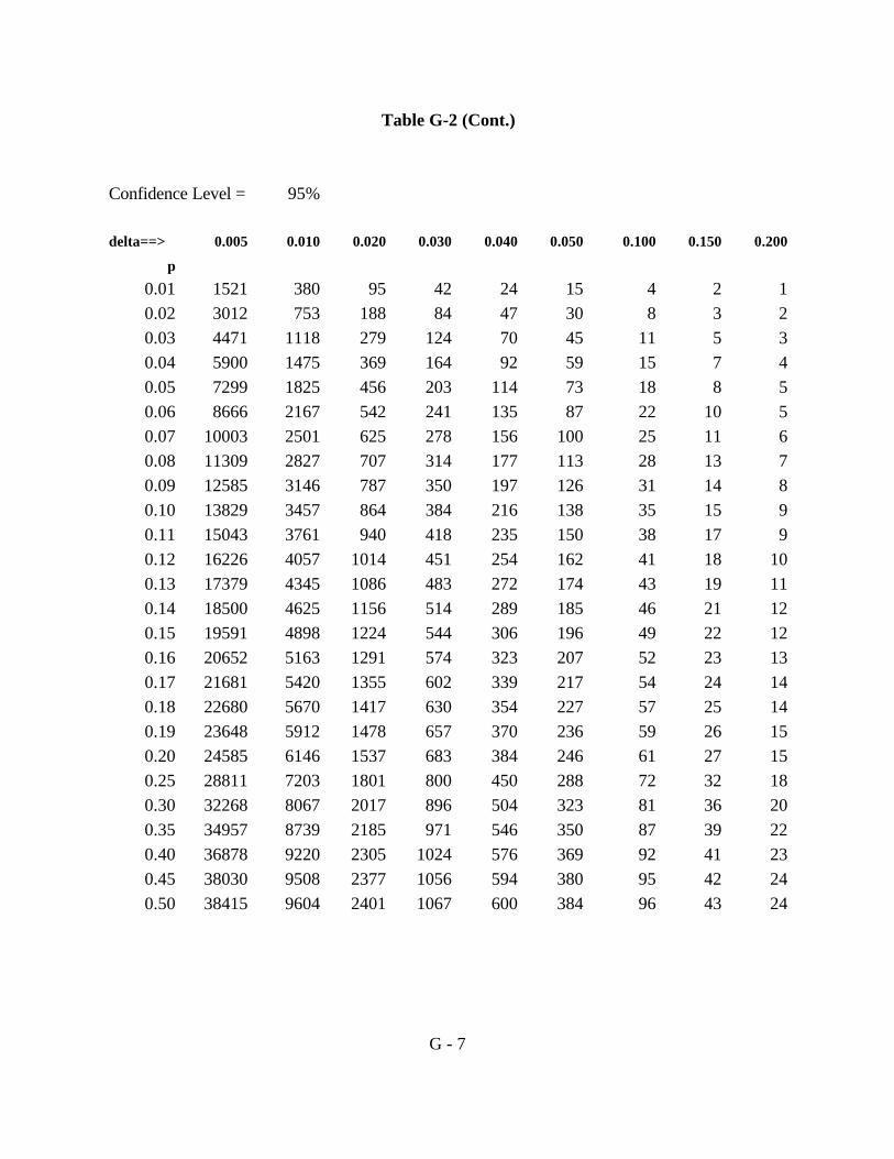
Table G-2 can be used to determine the minimum sample size needed to characterize thenumber of children with blood lead levels (BLLs) over 10 µg/dL. Table G-2 presents matrices forthe same four confidence levels. In the matrix corresponding to the desired level of confidenceyou would find the intersection between a proportion (p) above 10 µg/dL you believe the datawill have, and an acceptable margin of error delta (the deviation from the true value). Forexample, for a confidence level of 90 percent, believing the fraction of the population with bloodlead levels $ 10 µg/dL is 3 percent (0.03), you would need a sample size of 787 to achieve anaccuracy of + or - 0.01 of the true value.

Adjustment for Small Populations

Tables G-1 and G-2 serve to determine the initial uncorrected sample size for studying thegeometric mean and the proportion of the population above 10 µg/dL. However, when thepopulation being studied is smaller than the statistically valid sample size, an adjustment is madefor a finite population1.

For Table G-1 use the following:

n = n0 (N / (N+n0 )) where:n = the adjusted sample sizen0 = the statistically valid sample size from Table G-1N = the population size.

G - 2

For Table G-2 use the following:

n = n0 / (1 + (n0 / N)), where:n = the adjusted sample sizen0 = the statistically valid sample size from Table G-2N = the population size.

This information is provided to assist districts in the evaluation proposed study plans forblood lead sampling to establish site-specific blood lead distributions.

G - 3

Table G-1

Confidence Level = 80% 1.2815516

Acceptable multiple (>=1) of geometric mean

Geometric 1.050 1.100 1.200 1.300 1.400 1.500 1.600 2.000Standard Deviation

1.050 2 0 0 0 0 0 0 0

1.250 34 9 2 1 1 0 0 0

1.500 113 30 8 4 2 2 1 1

1.750 216 57 15 7 5 3 2 1

2.000 331 87 24 11 7 5 4 2

2.250 454 119 32 16 10 7 5 2

2.500 579 152 41 20 12 8 6 3

3.000 833 218 60 29 18 12 9 4

3.250 958 251 69 33 20 14 10 5




1.050 3 1 0 0 0 0 0 0

1.250 57 15 4 2 1 1 1 0

1.500 187 49 13 6 4 3 2 1

1.750 356 93 25 12 7 5 4 2

2.000 546 143 39 19 11 8 6 3

2.250 747 196 54 26 16 11 8 4

2.500 954 250 68 33 20 14 10 5

3.000 1372 359 98 47 29 20 15 7

3.250 1579 414 113 55 33 23 17 8

G - 4

Table G-1 (Cont.)




1.050 4 1 0 0 0 0 0 0

1.250 80 21 6 3 2 1 1 0

1.500 265 70 19 9 6 4 3 1

1.750 505 132 36 17 11 7 5 3

2.000 775 203 56 27 16 11 8 4

2.250 1061 278 76 37 22 15 11 5

2.500 1355 355 97 47 28 20 15 7

3.000 1948 510 139 67 41 28 21 10

3.250 2242 587 161 78 47 32 24 11




1.050 7 2 0 0 0 0 0 0

1.250 139 36 10 5 3 2 1 1

1.500 458 120 33 16 10 7 5 2

1.750 873 229 63 30 18 13 9 4

2.000 1339 351 96 46 28 19 14 7

2.250 1833 480 131 63 39 27 20 9

2.500 2340 613 168 81 49 34 25 12

3.000 3364 882 241 116 71 49 36 17

3.250 3872 1015 277 134 81 56 42 19

G - 5

Table G-2

Confidence Level = 80%

delta==> 0.005 0.010 0.020 0.030 0.040 0.050 0.100 0.150 0.200

p

0.01 650 163 41 18 10 7 2 1 1

0.02 1288 322 80 36 20 13 3 1 1

0.03 1912 478 119 53 30 19 5 2 1

0.04 2523 631 158 70 39 25 6 3 2

0.05 3121 780 195 87 49 31 8 3 2

0.06 3705 926 232 103 58 37 9 4 2

0.07 4277 1069 267 119 67 43 11 5 3

0.08 4835 1209 302 134 76 48 12 5 3

0.09 5380 1345 336 149 84 54 13 6 3

0.10 5913 1478 370 164 92 59 15 7 4

0.11 6432 1608 402 179 100 64 16 7 4

0.12 6937 1734 434 193 108 69 17 8 4

0.13 7430 1858 464 206 116 74 19 8 5

0.14 7910 1977 494 220 124 79 20 9 5

0.15 8376 2094 524 233 131 84 21 9 5

0.16 8829 2207 552 245 138 88 22 10 6

0.17 9270 2317 579 257 145 93 23 10 6

0.18 9697 2424 606 269 152 97 24 11 6

0.19 10110 2528 632 281 158 101 25 11 6

0.20 10511 2628 657 292 164 105 26 12 7

0.25 12318 3079 770 342 192 123 31 14 8

0.30 13796 3449 862 383 216 138 34 15 9

0.35 14946 3736 934 415 234 149 37 17 9

0.40 15767 3942 985 438 246 158 39 18 10

0.45 16260 4065 1016 452 254 163 41 18 10

0.50 16424 4106 1026 456 257 164 41 18 10

G - 6

Table G-2 (Cont.)


delta==> 0.005 0.010 0.020 0.030 0.040 0.050 0.100 0.150 0.200

p

0.01 1071 268 67 30 17 11 3 1 1

0.02 2121 530 133 59 33 21 5 2 1

0.03 3149 787 197 87 49 31 8 3 2

0.04 4156 1039 260 115 65 42 10 5 3

0.05 5141 1285 321 143 80 51 13 6 3

0.06 6104 1526 381 170 95 61 15 7 4

0.07 7045 1761 440 196 110 70 18 8 4

0.08 7965 1991 498 221 124 80 20 9 5

0.09 8863 2216 554 246 138 89 22 10 6

0.10 9740 2435 609 271 152 97 24 11 6

0.11 10595 2649 662 294 166 106 26 12 7

0.12 11428 2857 714 317 179 114 29 13 7

0.13 12240 3060 765 340 191 122 31 14 8

0.14 13030 3257 814 362 204 130 33 14 8

0.15 13798 3450 862 383 216 138 34 15 9

0.16 14545 3636 909 404 227 145 36 16 9

0.17 15270 3818 954 424 239 153 38 17 10

0.18 15974 3993 998 444 250 160 40 18 10

0.19 16655 4164 1041 463 260 167 42 19 10

0.20 17315 4329 1082 481 271 173 43 19 11

0.25 20292 5073 1268 564 317 203 51 23 13

0.30 22727 5682 1420 631 355 227 57 25 14

0.35 24620 6155 1539 684 385 246 62 27 15

0.40 25973 6493 1623 721 406 260 65 29 16

0.45 26785 6696 1674 744 419 268 67 30 17

0.50 27055 6764 1691 752 423 271 68 30 17

G - 7

Table G-2 (Cont.)


delta==> 0.005 0.010 0.020 0.030 0.040 0.050 0.100 0.150 0.200

p

0.01 1521 380 95 42 24 15 4 2 1

0.02 3012 753 188 84 47 30 8 3 2

0.03 4471 1118 279 124 70 45 11 5 3

0.04 5900 1475 369 164 92 59 15 7 4

0.05 7299 1825 456 203 114 73 18 8 5

0.06 8666 2167 542 241 135 87 22 10 5

0.07 10003 2501 625 278 156 100 25 11 6

0.08 11309 2827 707 314 177 113 28 13 7

0.09 12585 3146 787 350 197 126 31 14 8

0.10 13829 3457 864 384 216 138 35 15 9

0.11 15043 3761 940 418 235 150 38 17 9

0.12 16226 4057 1014 451 254 162 41 18 10

0.13 17379 4345 1086 483 272 174 43 19 11

0.14 18500 4625 1156 514 289 185 46 21 12

0.15 19591 4898 1224 544 306 196 49 22 12

0.16 20652 5163 1291 574 323 207 52 23 13

0.17 21681 5420 1355 602 339 217 54 24 14

0.18 22680 5670 1417 630 354 227 57 25 14

0.19 23648 5912 1478 657 370 236 59 26 15

0.20 24585 6146 1537 683 384 246 61 27 15

0.25 28811 7203 1801 800 450 288 72 32 18

0.30 32268 8067 2017 896 504 323 81 36 20

0.35 34957 8739 2185 971 546 350 87 39 22

0.40 36878 9220 2305 1024 576 369 92 41 23

0.45 38030 9508 2377 1056 594 380 95 42 24

0.50 38415 9604 2401 1067 600 384 96 43 24

G - 8

Table G-2 (Cont.)


delta==> 0.005 0.010 0.020 0.030 0.040 0.050 0.100 0.150 0.200

p

0.01 2627 657 164 73 41 26 7 3 2

0.02 5202 1300 325 144 81 52 13 6 3

0.03 7723 1931 483 215 121 77 19 9 5

0.04 10191 2548 637 283 159 102 25 11 6

0.05 12606 3152 788 350 197 126 32 14 8

0.06 14968 3742 936 416 234 150 37 17 9

0.07 17277 4319 1080 480 270 173 43 19 11

0.08 19533 4883 1221 543 305 195 49 22 12

0.09 21736 5434 1358 604 340 217 54 24 14

0.10 23886 5971 1493 663 373 239 60 27 15

0.11 25982 6496 1624 722 406 260 65 29 16

0.12 28026 7006 1752 778 438 280 70 31 18

0.13 30016 7504 1876 834 469 300 75 33 19

0.14 31954 7988 1997 888 499 320 80 36 20

0.15 33838 8459 2115 940 529 338 85 38 21

0.16 35669 8917 2229 991 557 357 89 40 22

0.17 37447 9362 2340 1040 585 374 94 42 23

0.18 39172 9793 2448 1088 612 392 98 44 24

0.19 40844 10211 2553 1135 638 408 102 45 26

0.20 42463 10616 2654 1180 663 425 106 47 27

0.25 49762 12440 3110 1382 778 498 124 55 31

0.30 55733 13933 3483 1548 871 557 139 62 35

0.35 60378 15094 3774 1677 943 604 151 67 38

0.40 63695 15924 3981 1769 995 637 159 71 40

0.45 65685 16421 4105 1825 1026 657 164 73 41

0.50 66349 16587 4147 1843 1037 663 166 74 41

Appendix H

Basis and Rationale for Risk Management Levels

H - 1

Appendix H

Basis and Rationale for Risk Management Levels

1. Risk Management Levels

In the permitting process, the districts make decisions about the need for controltechnology and whether new sources or modifications to existing sources can be permitted. Forthis purpose, the district identifies the following risk levels:

1) Toxic Best Available Control Technology (T-BACT) trigger level. This is the risklevel at which the district would require a source to install T-BACT on the newsource or the new equipment at an existing source.

2) Approvable level. Below this level, the district could approve a new source ormodification to an existing source without a Specific Findings Report.

3) Permit denial level. At a risk equal to or above this level, the district would notissue a permit.

For the Hot Spots Program, recommendations are needed for the following riskmanagement levels:

1) Notification level. This is the risk level at which facilities need to notify theexposed population (this could be the same as the significant risk level).

2) Significant risk level. At this level, facilities would be required to implement a riskreduction audit and plan. The risk reduction audit and plan must show how thefacility will reduce the risks to below this level within 5 years. The district maylengthen the implementation period up to an additional five years if that additionaltime will not result in an unreasonable risk and compliance within 5 years is nottechnically feasible and economically practicable .

3) Unreasonable risk level. Facilities with risks at or above this level must reducetheir risks within five years or less. The district may shorten the implementationperiod if it is technically feasible and economically practicable or if the emissionsfrom the facility pose an unreasonable risk.

2. Basis for Consideration of Risk Management Recommendations

The U.S. Department of Health and Human Services’ Centers for Disease Control andPrevention (CDC) has declared that the goal of all lead poisoning prevention activities should beto reduce children’s blood lead levels (BLLs) below 10 µg/dL (CDC, 1991). If many children in

H - 2

the community have BLLs $10 µg/dL, communitywide interventions (primary preventionactivities) should be considered by appropriate agencies. Interventions for individual childrenshould begin at BLLs of 15 µg/dL. There are a range of recommended actions based on theBLLs. Within the 15-19 µg/dL range of BLLs, a child should be given nutritional and educationalintervention and more frequent screening. If BLLs in this range persist, environmentalinvestigation and intervention are recommended. BLLs within the 20-44 µg/dL range trigger arecommendation for environmental investigation and intervention, and a medical evaluation. AtBLLs within the 45-69 µg/dL range, the recommendation is for both environmental and medicalintervention, including chelation therapy. BLLs over 70 µg/dL constitute a medical emergencyand require immediate environmental and medical intervention.

The Department of Toxic Substances Control (DTSC) in the California EnvironmentalProtection Agency has identified a one percent risk of exceeding 10 µg/dL as the “point ofdeparture”, i.e., starting point, for decisions about soil clean-up (DTSC, 1996). This might beconsidered to be analogous to a 1 in a million cancer risk, generally regarded as a level belowwhich no action need be taken. At levels above this, other factors such as land use, technicalfeasibility, or cost might be considered by DTSC in determining appropriate risk managementactions.

The United States Environmental Protection Agency (U.S. EPA) has been directed toestablish “screening levels” for lead in soil. The screening level is a level above which site-specificanalysis is recommended to establish clean-up goals. In considering what to set as screeninglevels, the U.S. EPA evaluated soil concentrations which would “pose a risk” to a typical (orhypothetical) child or group of similarly exposed children. The level U.S. EPA considered to“pose a risk” was defined as the concentration at which children had no more than a 5 percentchance of BLLs $ 10 µg/dL (U.S. EPA, 1998). In developing the residential screening level, theOffice of Solid Waste and Emergency Response (OSWER) applied the U.S. EPA’s IEUBK modelon a site-specific basis. The model generates a probability distribution of BLLs for a typical child,or group of children, exposed to a particular soil lead level and concurrent lead exposure fromother sources. This would be an individual risk for the child in a specific residence. This is anapproach that fits well with the purpose of determining whether the soil at a particular locationneeds to be removed or covered.

The federal Ambient Air Quality Standard (AAQS) for lead was originally set at a levelthat was designed to prevent 99.95 percent of children from exceeding a BLL of 25 µg/dL, whichwas at that time the level of concern. Using protection of 99.95 percent of children as aprecedent, it might be reasonable to base an assessment of significance on the percentage increasein the number of children expected to have BLLs $ 10 µg/dL. However, the data on currentblood lead levels in children indicate that this level of protection could not be achieved even ifthere were no exposure to lead in air because of the other sources of exposure which contributeto children’s BLLs.

H - 3

3. Rationale for the Risk Management Levels for the Simplified Approach

In consideration of the complexity of estimating risk for two different types of healtheffects using two different averaging times for the dispersion modeling, we are proposing analternative procedure. In this procedure, the 30-day average air concentration at the point ofmaximum impact would be compared to air concentrations representing risk management levels. We chose to use the 30-day average at the point of maximum impact because that makes thisapproach a little more conservative than the detailed approach for most facilities. For the HotSpots Program, 0.30 µg/m3 is recommended as the notification and significant risk level and 0.55µg/m3 as the unreasonable risk level. For permitting, 0.30 µg/m3 is recommended as theapprovable level and 0.55 µg/m3 as the permit denial level. We chose these air concentrations inconsideration of the recommended neurodevelopmental risk management levels and the associatedcardiovascular risk. They are moderately conservative for all sources except those impactingneighborhoods with a high potential for exposure from other sources. Therefore, we do notrecommend their use in areas that would fit the high exposure scenario for neurodevelopmentaleffects.

4. Rationale for the Risk Management Levels for Neurodevelopmental Effects

The precedents cited, thus far, are based on a calculation of individual risk. This is anappropriate approach for making decisions about whether to clean up the lead at an individualresidence or specific location. Risk management for lead emitted to the air from stationarysources differs from risk management for lead in soil. Soil lead is relatively stationary, while leademitted to the air from a stationary source can increase the exposure of a whole community. Airquality models are used to predict the location and concentration of the resulting lead in the airand are used to predict the point of maximum impact. However, the actual impact of airemissions on exposure cannot be predicted so precisely. In the case of lead, where thecontribution from the air lead may be small in comparison to the exposures from other sources, itmay be more realistic to evaluate the neurodevelopmental effects for an area rather than for the“maximally exposed individual”.

It is possible to calculate the change in the mean BLL for an exposed neighborhood orcommunity but there is little agreement about the significance of “averaged” increases in BLLs.Therefore, we are recommending that the risk (probability) of BLLs $ 10 µg/dL for the maximumexposure area be evaluated.

Hot Spots Program

The notification level for the Hot Spots Program is recommended at a 5 percent risk ofBLLs $ 10 µg/dL. This is consistent with U. S. EPA’s statement that a risk between 1 and 5percent probability “poses a threat” to children living in a lead contaminated home. The U.S.EPA also concluded that in the context of determining hazardous levels of lead in soil and dust, itwas not possible to distinguish between 1 and 5 percent risk due to the uncertainty and variability

H - 4

associated with relating lead in the environment to blood lead concentrations. To avoid asituation where all sources of lead located in or near a high exposure area would have to makenotification, we are recommending an alternative level that allows the consideration of the fractionof the mean BLL the facility contributes. In proposing the level for the facility contribution, weconsidered the other routes of exposure through water, soil, dust, and food. We believe the airlead should not contribute a disproportionate fraction of the risk. We also must consider that thesource doing a risk assessment for the Hot Spots Program will not be the only source of air lead. Notification is recommended to be required only for those with a facility contribution $ 10percent.

The significant risk level for an existing source in the Hot Spots Program is recommended to beset at the 5 percent risk of BLLs $ 10 µg/dL. This could present a problem for sources in an areawith a high potential for exposure due to other sources. In a high exposure scenario forneurodevelopmental effects, the background risk could be over the 5 percent risk of BLLs $ 10µg/dL. To avoid a situation in which a source would be required to reduce risks due to othersources, it is recommended the facility contribution is not allowed to exceed 10 percent of themean BLL in the neighborhood.

In considering what might constitute an unreasonable risk for the Hot Spots Program, wefound little regulatory precedent. In 1975, U.S. EPA set a maximum contaminant level for lead inwater of 0.05 milligrams per liter. This would result in a 20 percent risk of BLLs $ 10 µg/dL. This was re-evaluated in 1991 and the U.S. EPA declined to set a maximum contaminant levelbecause there is no known threshold below which lead health effects would not be expected. Inconsideration of risk levels associated with dangerous levels of lead, the highest probabilityconsidered by U.S. EPA was 10 percent. This level would be associated with a probability of 1.6percent that children would have a blood lead level $ 15 µg/dL. The U.S. EPA found thisunacceptable and we concur and are proposing a 10 percent risk of BLLs $ 10 µg/dL as theunreasonable risk level.

Permit Decisions

Several approaches were considered for setting a T-BACT trigger level. Because there isno safe threshold for neurodevelopmental effects of lead, we considered a zero T-BACT trigger. This approach would require any source seeking a permit for a new source or a modification thatwould emit lead to install T-BACT. Theoretically, this would require T-BACT for anymanufacturer that did small amounts of soldering or casting, for small combustion sources, or forany new firing range. We also considered setting a risk based T-BACT trigger level. Forinstance, a 1 percent individual risk of having a BLL $ 10 µg/dL similar to the DTSC’s “point ofdeparture” as discussed earlier. However, we believe a T-BACT trigger should apply to allfacilities equally, not depend on whether a new source was proposed for an area with a highpotential for exposure due to other sources.

H - 5

Another approach we considered was a T-BACT trigger level based on an airconcentration. An increase of 0.02 µg/m3 would double the average exposure based on thepopulation-weighted statewide ambient average concentrations. However, that approach wouldrequire a new source that emitted even very small quantities of lead to do air dispersion modeling.A simpler approach for both the sources and the districts would be a T-BACT trigger based on anemission rate. For sources with no stack, an emission rate of 1 pound per month could result in anair concentration of 0.02 µg/m3. Using this emission rate as the T-BACT trigger would ensure aconsistent level of protection and protection for children in neighborhoods with a high potentialfor exposure.

In terms of permitting, we believe that if a permit is issued for a source with risks abovethe significant level, the reasons for issuing the permit should be documented and made public. We further believe there should be a level above which a source should not be issued a permit. The U.S. EPA finds that a probability of BLLs $ 10 µg/dl between 1 and 5 percent poses a risk. However, they also found that it was not possible to reliably distinguish between a 1 percent and a5 percent probability. This was due to measurement variability, individual variability and theuncertainties in the modelling process. We considered these factors and the findings of theNHANES study (see Appendix A) that two percent of the children in the western region haveBLLs $ 10 µg/dl. These considerations lead us to recommend a probability of 5 percent as theapprovable level. Therefore, if the risk equals or exceeds 5 percent, a decision to permit thesource should be accompanied by a justification in a Special Findings Report issued by the district.

We are recommending the permit denial level be a 10 percent probability of BLLs$ 10 µg/dl. This is consistent with our recommended unacceptable level and was recommendedon the basis of similar considerations.

6. Rationale for the Risk Management Recommendations for Cancer

For cancer risk, we are proposing the same risk management levels as in the RiskManagement Guidance; a T-BACT trigger of 1 in a million, an approvable level of 10 in a millionand a permit denial level of 100 in a million. For the Hot Spots Program, we are proposing apublic notification level and significant risk level of 10 in a million and an unreasonable risk levelof 100 in a million.

Significance levels for cancer effects have evolved over the past several years. For manydistricts, less than 1 in a million cancer risk would not trigger use of toxics best available controltechnology (T-BACT). One hundred in a million, however, is generally considered unacceptablefor permitting purposes. Above the 1 in a million level, district new source toxic regulations oftenrequire installation of T-BACT. Districts generally require public notification in the Hot SpotsProgram at a cancer risk of 10 in a million. Individual districts have adopted significant risk levelsranging from 10 to 100 in a million but there is general agreement on an unreasonable risk level of100 in a million.

Appendix I

Specific Findings and a Specific Findings Report

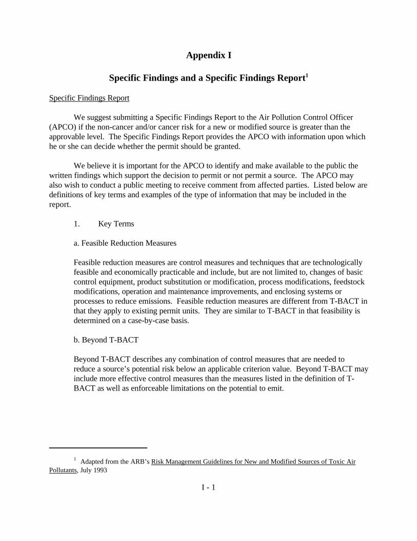
1 Adapted from the ARB’s Risk Management Guidelines for New and Modified Sources of Toxic AirPollutants, July 1993

I - 1

Appendix I

Specific Findings and a Specific Findings Report1

Specific Findings Report

We suggest submitting a Specific Findings Report to the Air Pollution Control Officer(APCO) if the non-cancer and/or cancer risk for a new or modified source is greater than theapprovable level. The Specific Findings Report provides the APCO with information upon whichhe or she can decide whether the permit should be granted.

We believe it is important for the APCO to identify and make available to the public thewritten findings which support the decision to permit or not permit a source. The APCO mayalso wish to conduct a public meeting to receive comment from affected parties. Listed below aredefinitions of key terms and examples of the type of information that may be included in thereport.

1. Key Terms

a. Feasible Reduction Measures

Feasible reduction measures are control measures and techniques that are technologicallyfeasible and economically practicable and include, but are not limited to, changes of basiccontrol equipment, product substitution or modification, process modifications, feedstockmodifications, operation and maintenance improvements, and enclosing systems orprocesses to reduce emissions. Feasible reduction measures are different from T-BACT inthat they apply to existing permit units. They are similar to T-BACT in that feasibility isdetermined on a case-by-case basis.

b. Beyond T-BACT

Beyond T-BACT describes any combination of control measures that are needed toreduce a source’s potential risk below an applicable criterion value. Beyond T-BACT mayinclude more effective control measures than the measures listed in the definition of T-BACT as well as enforceable limitations on the potential to emit.

I - 2

2. Content

a. Identify pollutants that would be emitted.

The report should identify and quantify the toxic air pollutants that would beemitted from the source.

b. Identify the health impact of the toxic pollutant(s) that would be emitted.

The cancer and non-cancer risk associated with the toxics that would be emittedfrom the new or modified source should be identified and discussed. The applicantmay also wish to discuss potential cancer burden as a measure of communicatingthe magnitude of the potential cancer risk. As specified in the CAPCOA AirToxics “Hot Spots” Program Risk Assessment Guidelines, (October, 1993) thepermit applicant should also discuss how currently undeveloped areas are “zoned”(i.e. commercial or residential) and use this information to estimate potential healthimpacts should this area be developed. The applicant may wish to presentinformation on the likelihood that an individual could reside at the point ofmaximum off-site cancer risk.

c. Discuss the uncertainty in the risk assessment process.

The permit applicant may wish to include information regarding uncertainty in therisk assessment process as described in the chemical health effects documents.

d. Discuss the benefits associated with the new or modified source.

The permit applicant may wish to include information regarding the benefit thenew or modified source would provide the local community. Benefits of thesource may include the service provided to the community or a decrease in riskcompared to risk estimates without the source.

e. Identify federal, state, or local mandates.

The permit applicant may indicate whether there are any existing federal, state, orlocal mandates that requires modification of an existing source or establishment ofa new source. For example, the state’s clean fuel regulations may require anexisting gasoline station to offer clean fuel for sale. In order to comply, the ownerof the gasoline station may have to modify the facility to add a clean fuel pump.

I - 3

f. Identify multi-media impacts.

The APCO should require the permit applicant to identify the impact the new ormodified source may have on media other than air.

g. Discuss the findings of the California Environmental Quality Act (CEQA)document if one was required for the project.

Independent of these guidelines, the APCO must review environmental impactreports (EIRs) that are prepared by the Lead Agency pursuant to the requirementsof the CEQA. This document should provide information regarding background,cumulative, and ecological risk. Background risk is the risk associated with theambient toxic air pollutant levels due to local stationary sources and mobilesources. Cumulative risk is the sum of the risk of toxic air pollutant emissionsfrom local stationary sources within a given area. Ecological risk is the risk toflora and fauna resulting from emissions of toxic air pollutants.

h. Identify sensitive receptors impacted by the new or modified source.

The APCO may require the permit applicant to identify any sensitive receptorlocations impacted by the toxic air emissions from the new or modified source. Asensitive receptor location includes, but is not limited to, any hospital, school, orday-care center.

i. Provide a risk reduction plan.

The APCO may require, or the permit applicant may wish to provide, a riskreduction plan identifying all feasible reduction measures to reduce potential riskfrom the source.

The risk reduction plan should:

i. Identify which processes and activities cause toxic emissions andwhat portion of the total potential source risk is due to each.

ii. Identify all feasible reduction measures and applicable beyond T-BACT measures for the source type.

iii. Estimate the risk reduction potential of the feasible reductionmeasures and beyond T-BACT measures.

iv. Estimate how long it would take to implement the feasiblereduction measures and beyond T-BACT measures.

I - 4

v. Determine the technical feasibility and cost-effectiveness of thefeasible reduction measures and beyond T-BACT measures for theindividual source.

vi. Identify the feasible reduction measures and beyond T-BACTmeasures that will be implemented to reduce potential risk and adetailed schedule for implementation. If the plan shows that thesemeasures are insufficient to meet the lower risk level, the planshould identify possible reductions in the future.

Appendix J

Regulatory Programs for Lead

1 The State Department of Public Health is now the Department of Health Services (DHS)

June 27, 2001 J - 1

Appendix J

Regulatory Programs for Lead

This Appendix presents a summary of past regulatory approaches and actions on airbornelead. It also discusses regulatory programs established to address toxic air contaminants.

Ambient Air Quality Standards

An ambient air quality standard (AAQS) is a regulation designed to protect public healthby establishing an allowable air concentration of a pollutant. There are both State and Federal airquality standards for lead. The State AAQS for lead was established in November 1970 followingthe recommendations of the State Department of Public Health1. It was based on health effectsdata that showed exposure to airborne lead levels above 1.5 micrograms per cubic meter (µg/m3)averaged over a 30-day period could result in the accumulation of lead in the body in quantitiessufficient to cause impairment of the blood forming system.

The federal standard was set at 1.5 micrograms per cubic meter (µg/m3) averaged over a90-day period. The federal standard was set at a level that would insure that 99.5 percent ofchildren would have a BLL less than 40 micrograms per deciliter (µg/dL). At that time, 40 µg/dLwas considered to be an elevated BLL.

As better data on health effects were developed, public health agencies revised downwardthe BLL of concern. By 1991, the Centers for Disease Control and Prevention (CDC) of the U.S.Department of Health & Human Services, Public Health Service considered 10 µg/dl to be anelevated BLL in children. The CDC recommends community intervention (primary preventionactivities by the appropriate agencies) if many children in the community have BLLs at or overthis level. An example of a primary prevention activity is clean-up of a site with soilcontamination even if it has not been established that the site has contributed to the high BLLsdetected. The Office of Environmental Health Hazard Assessment (OEHHA) has identified 10µg/dl as a level of concern because it is a level at which studies have adequately demonstrated anadverse health effect.

When the Air Resources Board (ARB/Board) reviewed the State AAQS in 1985, changeswere made to the measurement methods but the standard was left at 1.5 µg/m3 over a 30-dayaveraging time. The United States Environmental Protection Agency (U.S. EPA) reviewed thefederal AAQS in 1990 and did not revise it. It remains at 1.5 µg/m3 over a 90-day averagingtime.

June 27, 2001 J - 2

The Toxic Air Contaminant Identification and Control Program

Assembly Bill 1807 (1983) established a program for the identification and control of toxicair contaminants. In this program, risk assessment is separated from risk management. Riskassessment is the process of examining the available evidence on health effects associated withexposure to a substance and relating the probability of adverse health effects to a given exposurelevel. Risk management is the process of evaluating emission sources to determine the need andappropriate degree of regulation, and if necessary, taking action to reduce emissions.

Under the AB 1807 air toxics identification phase (risk assessment), ARB and OEHHAstaffs prepare a report for public review that is the basis for the proposed identification of asubstance as a toxic air contaminant (TAC). The identification process involves full publicparticipation including numerous comment periods, workshops, meetings with affected industries,a review by the independent Scientific Review Panel (SRP), and consideration by the Board at aformal public hearing.

Once a substance has been formally identified as a TAC, the risk management phasebegins. In the risk management process, ARB staff conduct a regulatory needs assessment. A“needs assessment” is an assessment of the need and appropriate degree of regulation for asubstance identified as a TAC. Full public participation is also a feature of the risk managementprocess. ARB staff carries out this evaluation in consultation with the districts, affected sources,and the interested public. Typically, the ARB publishes a report that describes the regulatoryneeds assessment and summarizes staff recommendations for actions.

The following issues are considered to the extent that data can reasonably be madeavailable:

1. current and future anticipated emission rates, levels of human exposure, and therisk associated with those levels;

2. the stability, persistence, transformation products, dispersion potential, andphysical and chemical characteristics of the substance when present in the ambientair;

3. the categories, numbers, and relative contribution of present or anticipated sourcesof the substance;

4. the availability and technological feasibility of control measures, taking intoaccount the effect of control measures on levels of exposure, and recenttechnological improvements or other actions which emitting sources haveimplemented in the recent past to reduce emissions;

5. the cost and cost effectiveness of control measures;6. the availability, suitability, and efficacy of substitute compounds of a less

hazardous nature; and7. the potential adverse health, safety, or environmental impacts of implementing a

control measure.

June 27, 2001 J - 3

The Board considers the recommendations made in the regulatory needs assessment.When this analysis indicates a need for additional control, staff--subsequent to Board approval--develop, in cooperation with industry and districts, a proposed control measure for considerationby the Board. In a formal hearing, the Board considers public comments, receives publictestimony, and acts on the proposal. Once the statewide control measure is adopted, the districtsimplement and enforce it, or adopt and enforce one at least as stringent.

The status of lead under AB 1807

ARB and OEHHA evaluated lead for identification as a toxic air contaminant (TAC)under the AB 1807 program. The Board approved the listing of inorganic lead as a TAC at apublic hearing April 24, 1997. Lead was listed as a TAC for which a threshold exposure levelcould not be identified. The threshold exposure level is the level below which adverse healtheffects are not expected to occur. Lead is the first identified TAC for which non-cancer effectswith no threshold have been identified. At that hearing, the Board directed ARB staff to developrisk management guidance to assist districts and industry to evaluate the potential health effects oflead emissions.

The OEHHA’s review of available health effects data published in the March 1997“Technical Support Document, Proposed Identification of Inorganic Lead as a Toxic AirContaminant, Part B Health Assessment” examined and reported on many studies. The OEHHAnoted that a recent study specifically focused on determining a threshold was unable to detect one. The ARB, SRP, and OEHHA concur in the conclusion that a “no observed adverse effect level”(NOAEL) cannot be reliably identified for at least three of the health effects of lead: cancer,cardiovascular effects in adults, and neurological impairment in children. Other reviews of healthoutcomes associated with lead exposure can be found in the U.S. EPA’s “Air Quality Criteria forLead”, published in 1986, and “Air Quality Criteria for Lead: Supplement to the 1986Addendum”, published in 1990; the Agency for Toxic Substances and Disease Registry’s“Toxicological Profile for Lead”, published in 1990 (currently being revised); and the NationalResearch Council’s “Measuring Lead Exposure in Infants, Children, and Other SensitivePopulations”, published in 1993.

Regulations affecting lead adopted under AB 1807

Following the identification of cadmium as a toxic air contaminant in January 1987, ARBstaff developed an airborne toxic control measure (ATCM) for emissions of toxic metals fromnon-ferrous metal melting operations. The Board adopted the ATCM in January 1993. It iscurrently being implemented by affected facilities and by the districts. Because lead is emittedfrom some of the same facilities that the ATCM affects, lead emissions were also reduced as aresult of compliance with that regulation. This is because the ATCM requires reduction inemissions of particulate matter, in which cadmium, lead, and other metals occur.

June 27, 2001 J - 4

Need for additional regulations to reduce lead emissions

The ARB staff is currently conducting an evaluation of lead sources, emissions, and risk todetermine whether additional control measures are needed for lead. The findings of thatassessment will determine staff recommendations as to whether additional actions are necessary.

The Air Toxics “Hot Spots” Program

Assembly Bill (AB) 2588 established the Air Toxics “Hot Spots” Information andAssessment Act (Air Toxics “Hot Spots” Program) in 1987. AB 2588 established requirementsfor facilities to report their emissions of air toxics including lead. The districts review thesereports and then prioritize the facilities based on their potential health risk. Risk assessments areperformed for high priority facilities. Facilities with risks that exceed district-specified triggerlevels must notify the public. To facilitate risk assessment review and improve statewideconsistency, the California Air Pollution Control Officer’s Association (CAPCOA) published riskassessment guidelines.

In 1992, additional requirements were added through adoption of Senate Bill (SB) 1731. The objective of SB 1731 was to require facilities with significant risks to reduce their risks. SB 1731 requires local air districts to designate significant risk levels. Facilities with risks overthe significance level are then required to develop a risk reduction audit and plan describingactions they will take to reduce their risks. SB 1731 also directed OEHHA to develop riskassessment guidelines. Finally, SB 1731 directed the ARB to provide assistance to the districtsand smaller businesses. To that end, the ARB has produced a general guideline document for allfacilities on how to conduct a risk reduction audit and prepare a risk reduction plan, and source-specific guideline documents for chrome plating, aerospace operations, degreasing operations, andautobody shops.

Other Actions to Reduce Lead Exposure

There have been several regulatory actions taken in the last 10 years which havesignificantly reduced the public’s exposure to lead. Both the ARB and U.S. EPA have acted toreduce lead use in gasoline. The U.S. EPA promulgated a National Emissions Standards forHazardous Air Pollutants (NESHAP) for Secondary Lead Smelting in 1995 which imposed limitson emissions from stacks and required improved housekeeping and operating procedures toreduce fugitive emissions. The U.S. EPA has promulgated national primary drinking waterregulations for controlling lead in drinking water. The U.S. Consumer Products SafetyCommission has promulgated limits on lead in consumer products and in paint. These actionshave reduced the body burden of lead for U.S. residents. The quantitative effect can be seen inthe results of the National Health and Nutritional Examination Surveys (NHANES) whichmeasured blood lead levels at intervals since 1988. See Appendix A for a discussion of thefindings of the NHANES studies.

Appendix K

Form for Reporting a Planned Tier II Studyto the Childhood Lead Poisoning Prevention Branch

STATE OF CALIFORNIAHEALTH AND HUMAN SERVICES AGENCY GRAY DAVIS, Governor

DEPARTMENT OF HEALTH SERVICESCHILDHOOD LEAD POISONING PREVENTION BRANCH 1515 CLAY STREET, SUITE 1801OAKLAND, CA 94612 (510) 622-5000

SITE-SPECIFIC ENVIRONMENTAL SAMPLINGAT RESIDENTIAL ADDRESSES NEAR A STATIONARY SOURCE FACILITY

Tier II Data for Permit Application

Please complete this information and fax to Environmental Investigations Unit: (510) 622-5002

1. Complete the following Facility information:

NAME OF FACILITYADDRESS OF FACILITYCONTACT NAME/TITLECONTACT PHONE/FAXLOCAL APC DISTRICTAPCD CONTACT NAME/PHONELOCAL HEALTH OFFICERDATE HEALTH OFFICER NOTIFIED

2. Complete the following environmental sampling information:

DATE SAMPLING TO BE CONDUCTEDTOTAL NUMBER OF ADDRESSES TO BE SAMPLEDTOTAL NUMBER OF SOIL SAMPLES TO BE COLLECTEDTOTAL NUMBER OF DUST SAMPLES TO BE COLLECTEDTOTAL NUMBER OF WATER SAMPLES TO BE COLLECTEDTOTAL NUMBER OF FOOD SAMPLES TO BE COLLECTED

3. Attach a table that includes the following information:

EACH ADDRESS TO BE SAMPLEDSOIL SAMPLE LOCATIONSSOIL SAMPLE RESULTSDUST SAMPLE LOCATIONSDUST SAMPLE RESULTSWATER SAMPLE LOCATIONSWATER SAMPLE RESULTSTYPE OF FOOD SAMPLED AND RESULTS

4. Explain what steps the Facility will take for environmental results that exceed regulatory levels.

5. Explain how the Property Owner will be notified of lead contaminated soil, dust, and water.DHS CLPPB 5/30/00

Appendix A Environmental Lead and Exposure Trends · PDF file · 2006-06-21A - 1...

Documents

Transcript of Appendix A Environmental Lead and Exposure Trends · PDF file · 2006-06-21A - 1...