www.elsevier.com/locate/patrec

Pattern Recognition Letters 27 (2006) 618–626

Appearance-based gender classification with Gaussian processes

Hyun-Chul Kim a,*, Daijin Kim b, Zoubin Ghahramani c, Sung Yang Bang b

a Department of Industrial and Management Engineering, POSTECH, Pohang University of Science and Technology, San 31,

Hyoja Dong, Nam Gu, Pohang 790-784, South Koreab Department of Computer Science and Engineering, POSTECH, Pohang 790-784, South Korea

c Gatsby Computational Neuroscience Unit, UCL, London WC1N 3AR, UK

Received 11 August 2004; received in revised form 15 September 2005Available online 18 November 2005

Communicated by Y.J. Zhang

Abstract

This paper concerns the gender classification task of discriminating between images of faces of men and women from face images. Inappearance-based approaches, the initial images are preprocessed (e.g. normalized) and input into classifiers. Recently, support vectormachines (SVMs) which are popular kernel classifiers have been applied to gender classification and have shown excellent performance.SVMs have difficulty in determining the hyperparameters in kernels (using cross-validation). We propose to use Gaussian process clas-sifiers (GPCs) which are Bayesian kernel classifiers. The main advantage of GPCs over SVMs is that they determine the hyperparametersof the kernel based on Bayesian model selection criterion. The experimental results show that our methods outperformed SVMs withcross-validation in most of data sets. Moreover, the kernel hyperparameters found by GPCs using Bayesian methods can be used toimprove SVM performance.� 2005 Elsevier B.V. All rights reserved.

Keywords: Gender classification; Appearance-based gender classification; Kernel machines; Gaussian process classifiers; Support vector machines

1. Introduction

The face is a characteristic feature of human beingswhich contains identity and emotion. It is possible to iden-tify a person and her/his characteristics such as emotion (orexpression) and gender from her/his face. Recognizinghuman gender is important since lots of social interactionsand services depend on the gender. People respond differ-ently according to gender. Human computer interactionsystem can be more user-friendly and more human-likewhen it considers the user�s gender.

There are two main approaches for gender classification.The first approach is the appearance-based approach whichuses a whole face image. Cottrell and Metcalfe (1991)

0167-8655/$ - see front matter � 2005 Elsevier B.V. All rights reserved.

doi:10.1016/j.patrec.2005.09.027

* Corresponding author. Tel.: +82 562 279 8075; fax: +82 562 279 2299.E-mail address: grass@postech.ac.kr (H.-C. Kim).

reduced the dimension of whole face images by autoen-coder network and classified gender based on the reducedinput features. Golomb et al. (1991) used a two-layer neu-ral network (called SexNet) without dimensionality reduc-tion. Tamura et al. (1996) used a neural network andshowed that even very low resolution image such as 8 · 8can be used for gender classification. Gutta et al. (2000)used the mixture of experts with ensembles of radial basisfunctions (RBF) networks and a decision tree as a gatingnetwork. Moghaddam and Yang (2002) showed that sup-port vector machines (SVMs) worked better than otherclassifiers such as ensemble of RBF networks, classicalRBF networks, Fisher linear discriminant, nearest neigh-bor etc. Jain and Huang (2004) extracted wholistic featuresby independent component analysis (ICA) and classified itwith linear discriminant analysis (LDA). Costen et al.(2004) used the exploratory basis pursuit classificationwhich is a sparse kernel classifier.

H.-C. Kim et al. / Pattern Recognition Letters 27 (2006) 618–626 619

The second approach is the geometrical feature basedapproach. Burton et al. (1993) extracted point-to-point dis-tances from 73 points on face images and used discriminantanalysis as a classifier. Brunelli and Poggio (1992) extracted16 geometric features such as eyebrow thickness and pupil-to-eyebrow distance and used HyperBF networks as aclassifier.

As mentioned above, the appearance-based approachwith SVM showed excellent performance (Moghaddamand Yang, 2002). In their experiments the Gaussian kernelworked better than linear or polynomial kernels. They didnot mention how to set the hyperparameters1 for Gaussiankernel which have an influence on performance, but justshowed the test results with several different hyperpara-meters. Learning the hyperparameters should be includedin the training process. A standard way to determine thehyperparameters is by cross-validation. Alternatively wecould use kernel classifiers such as Gaussian process classi-fiers which automatically incorporate method to determinethe hyperparameters. In this paper we propose to useGaussian process classifiers (GPCs) for appearance-basedgender classification.

GPCs are a Bayesian kernel classifier derived fromGaussian process priors over functions which were devel-oped originally for regression (O�Hagan, 1978; Neal,1997; Williams and Barber, 1998; Gibbs and MacKay,2000). In classification, the target values are discrete classlabels. To use Gaussian processes for binary classification,the Gaussian process regression model can be modified sothat the sign of the continuous latent function it outputsdetermines the class label. Observing the class label at somedata point constrains the function value to be positive ornegative at that point, but leaves it otherwise unknown.To compute predictive quantities of interest we thereforeneed to integrate over the possible unknown values of thisfunction at the data points.

Exact evaluation of this integral is computationallyintractable. However, several successful methods have beenproposed for approximately integrating over the latentfunction values, such as the Laplace approximation (Wil-liams and Barber, 1998), Markov Chain Monte Carlo(Neal, 1997), and variational approximations (Gibbs andMacKay, 2000). Opper and Winther (2000) used theTAP2 approach originally proposed in statistical physicsof disordered systems to integrate over the latent values.The TAP approach for this model is equivalent to the moregeneral expectation propagation (EP) algorithm forapproximate inference (Minka, 2001). The expectationmaximization–expectation propagation (EM–EP) algo-rithm has been proposed to learn the hyperparametersbased on EP (Kim and Ghahramani, 2003). GPCs withthe hyperparameters obtained by the EM–EP algorithm

1 Hyperparameters control properties of the kernel and the amount ofclassification noise.2 TAP is an abbreviation of its developers� names such as Thouless,

Anderson and Palmer.

have shown better performance than SVMs which hadthe hyperparameters set by cross-validation, on most ofdata sets tested. In many cases the hyperparameters deter-mined by the EM–EP algorithm were more suitable forSVMs than the ones determined by cross-validation tech-nique. In this paper we use the EM–EP algorithm to learnGaussian process classifiers for gender classification. Weexpect that GPCs with the EM–EP algorithm work betterthan SVMs with the cross-validation and provide betterhyperparameters for the kernels of SVMs.

The paper is organized as follows. Section 2 introducesappearance-based gender classification. In Section 3, weintroduce Gaussian process classification. In Section 4,we describe the EP method and the EM–EP algorithmfor Gaussian process classification. In Section 5, we showexperimental results on the PF01 database and comparedwith other classification methods including SVMs. In Sec-tion 6, we draw conclusions and remark on future work.

2. Appearance-based gender classification

The appearance-based approach to gender classificationdiscriminates between male and female classes from faceimages without first explicitly extracting any geometricalfeatures. A typical way to do this is to train a classifier withtraining images and to classify new images by the trainedclassifier. Face images should be well-aligned so that facialfeatures are in the same positions. Since gender classifica-tion is a two-class classification problem, any kind of bin-ary classifier can be deployed.

Fig. 1 shows the process of appearance-based genderclassification. Assume that a classifier has been alreadytrained with some images in advance. The whole processof gender classification can be explained by the following.First, images are captured. Then, the captured images arepreprocessed by face detection and facial feature extractionalgorithms and cropped by an appropriate cropping tech-nique. The preprocessed face images can include a wholeoutline of faces with hair or can include only inner faceparts with only facial features. Then, the preprocessedimage (pixel-level features) is applied to the classifier andthe classifier determines the gender of the input image.

The appearance-based approach has two main advanta-ges. First, it preserves appearance of face images which canbe considered to be naive features. It is difficult to deter-mine what kind of geometrical features we should useand to tell the meaning of those features. In contrast tothis, appearance-based approach is more natural since ituses face images themselves. The benefit in being naturalis that it could make it easier to do what the natural beingdoes. Second, it does not need to extract facial features orpoints very accurately. To get good geometrical features,we need to know quite accurate facial feature or point loca-tions which requires accurate facial feature extraction. Incontrast to this, we need to know relatively small numberof facial features for alignment in the appearance-basedapproach. The disadvantages of the appearance-based

Fig. 1. The process of appearance-based gender classification.

620 H.-C. Kim et al. / Pattern Recognition Letters 27 (2006) 618–626

approach is that it has more features than the geometricalfeature based approach and that it does not provide a goodexplanation why a facial image is classified as a male orfemale.

We follow the above process for appearance-based gen-der classification and use Gaussian process classifiers.

3. Gaussian process classifiers

Let us assume that we have a data set D of data pointsxi with binary class labels yi 2 {�1,1}: D = {(xi,yi)ji =1,2, . . . ,n}, X = {xiji = 1,2, . . . ,n}, Y = {yiji = 1,2, . . . ,n}.Given this data set, we wish to find the correct class labelfor a new data point ~x. We do this by computing the classprobability pð~yj~x;DÞ.

We assume that the class label is obtained by transform-ing some real valued latent variable ~f , which is the value ofsome latent function f (Æ) evaluated at ~x. We put a Gaussianprocess prior on this function, meaning that any number ofpoints evaluated from the function have a multivariateGaussian density (see Williams and Rasmussen (1995) fora review of GPs). Assume that this GP prior is parameter-ized by H which we will call the hyperparameters. We canwrite the probability of interest given H as

pð~yj~x;D;HÞ ¼Z

pð~yj~f ;HÞpð~f jD; ~x;HÞ; d~f . ð1Þ

This is the probability of the class label ~y at a new datapoint ~x given data D and hyperparameters H.

The second part of Eq. (1) is obtained by further inte-gration over f = [f1, f2, . . . , fn], the values of the latent func-tion at the data points.

pð~f jD; ~x;HÞ ¼Z

pðf ; ~f jD; ~x;HÞdf

¼Z

pð~f j~x; f ;HÞpðf jD;HÞdf ; ð2Þ

where pð~f j~x; f ;HÞ ¼ pð~f ; f j~x;X ;HÞ=pðf jX ;HÞ and

pðf jD;HÞ / pðY jf ;X ;HÞpðf jX ;HÞ

¼Yni¼1

pðyijfi;HÞ( )

pðf jX ;HÞ. ð3Þ

The first term in Eq. (3) is the likelihood: the probabilityfor each observed class given the latent function value,while the second term is the GP prior over functions eval-

uated at the data. Writing the dependence of f on x implic-itly, the GP prior over functions can be written

pðf jX ;HÞ ¼ 1

ð2pÞN=2jCHj1=2

� exp � 1

2ðf � lÞ>C�1

H ðf � lÞ� �

; ð4Þ

where the mean l is usually assumed to be the zero vector 0and each term of a covariance matrix Cij is a function of xiand xj, i.e. c(xi,xj).

One form for the likelihood term p(yijfi,H), which relatesf(xi) monotonically to probability of yi = +1, is

pðyijfi;HÞ ¼ 1ffiffiffiffiffiffi2p

pZ yif ðx iÞ

�1exp � z2

2

� �dz ¼ erfðyif ðxiÞÞ.

ð5ÞOther possible forms for the likelihood are a sigmoid func-tion 1/(1 + exp(�yif(xi))), a step function H(yif(xi)), and astep function with a labelling error � + (1 � 2�)H(yif(xi)).

Since p(fjD,H) in Eq. (3) is intractable due to the non-linearity in the likelihood terms, we use an approximatemethod. Laplace approximation, variational methods andMarkov Chain Monte Carlo method were used in (Wil-liams and Barber, 1998; Gibbs and MacKay, 2000; Neal,1997), respectively. Expectation propagation, which isdescribed in the next section, was used in (Opper andWinther, 2000; Minka, 2001).

4. The EM–EP algorithm for GPCs

4.1. Expectation propagation for GPCs

The expectation-propagation (EP) algorithm is anapproximate Bayesian inference method (Minka, 2001).We review EP in its general form before describing itsapplication to GPCs.

Consider a Bayesian inference problem where the pos-terior over some parameter / is proportional to the priortimes likelihood terms for an i.i.d. data set

pð/jy1; . . . ; ynÞ / pð/ÞYni¼1

pðyij/Þ. ð6Þ

We approximate this by

qð/Þ / ~t0ð/ÞYni¼1

~tið/Þ; ð7Þ

H.-C. Kim et al. / Pattern Recognition Letters 27 (2006) 618–626 621

where each term (and therefore q) is assumed to be in theexponential family. EP successively solves the followingoptimization problem for each i

~tnewi ð/Þ ¼ argmin~tið/Þ

KLqð/Þ~toldi ð/Þ

pðyij/Þqð/Þ~toldi ð/Þ

����� ~tið/Þ !

; ð8Þ

where KL is the Kullback–Leibler divergence and

KLðpðxÞkqðxÞÞ ¼Z

pðxÞ log pðxÞqðxÞ dx. ð9Þ

Since q is in the exponential family, this minimization issolved by matching moments of the approximated distribu-tion. EP iterates over i until convergence. The algorithm isnot guaranteed to converge although it did in practice in allour examples and has worked well for many other authors.Assumed density filtering (ADF) is a special online form ofEP where only one pass through the data is performed(i = 1, . . . ,n).

We describe EP for GPC referring to (Minka, 2001;Opper and Winther, 2000). The latent function f playsthe role of the parameter / above. The form of the likeli-hood we use in the GPC is

pðyijfiÞ ¼ �þ ð1� 2�ÞHðyifiÞ; ð10Þwhere H(x) = 1 if x > 0, and otherwise 0. The hyperparam-eter, � in Eq. (10) models labeling error outliers. The EPalgorithm approximates the posterior p(fjD) = p(f)p(Djf)/p(D) as a Gaussian having the form qðf Þ � Nðmf ;Vf Þ,where the GP prior pðf Þ � Nð0;CÞ has covariance matrixC with elements Cij defined by the covariance function

Cij ¼ cðx i; xjÞ

¼ v0 exp � 1

2

Xdm¼1

lmdmðxmi ; xmj Þ( )

þ v1 þ v2dði; jÞ; ð11Þ

where xmi is the mth element of xi, and dmðxmi ; xmj Þ ¼ðxmi � xmj Þ

2 if xm is continuous; 1� dðxmi ; xmj Þ if x is discrete,where dðxmi ; xmj Þ is 1 if xmi ¼ xmj and 0 if xmi 6¼ xmj . The hyper-parameter v0 specifies the overall vertical scale of variationof the latent values, v1 the overall bias of the latent valuesfrom zero mean, v2 the latent noise variance, and lm the (in-verse) lengthscale for feature dimension m. The erf likeli-hood term in Eq. (5) is equivalent to using the thresholdfunction in Eq. (10) with � = 0 and non-zero latent noise v2.

EP tries to approximate pðf jDÞ ¼ pðf Þ=pðDÞQn

i¼1pðyijf Þ,where pðf Þ � N(0,C). p(yijf) = ti(f) is approximated by~tiðf Þ ¼ si expð� 1

2viðfi � miÞ2Þ. From this initial setting, we

can derive EP for GPC by applying the general ideadescribed above. The resulting EP procedure is virtuallyidentical to the one derived in (Minka, 2001). We definethe following notation3: K ¼ diagðv1; . . . ; vnÞ; hi ¼ E½fi�; hnii ¼E½f ni

i �, where hnii and f nii are quantities obtained from awhole

set except for xi. The EP algorithm is as follows which we

3 diag(v1, . . . ,vn) means a diagonal matrix whose diagonal elements arev1, . . . ,vn. Similarly for diag(v).

repeat for completeness—please refer to Minka (2001) forthe details of the derivation. After the initialization vi = 1,mi = 0, si = 1, hi = 0, ki = Cii, the following process is per-formed until all (mi,vi, si) converge.

Loop i = 1,2, . . . ,n:

(1) Remove the approximate density ~ti (for ith datapoint) from the posterior to get an �old� posterior:hnii ¼ hi þ kiv�1

i ðhi � miÞ.(2) Recompute part of the new posterior: z ¼ yih

niiffiffiffiki

p ;Zi ¼

�þ ð1� 2�ÞerfðzÞ ai ¼ 1ffiffiffiki

p ð1�2�ÞNðz;0;1Þ�þð1�2�ÞerfðzÞ ; hi ¼ hnii þ kiai,

where erf(z) is a cumulative normal density function.

(3) Get a new ~ti : vi ¼ kið 1aihi

� 1Þ;mi ¼ hi þ viai; si ¼Zi

ffiffiffiffiffiffiffiffiffiffiffiffiffiffiffiffiffiffiffi1þ v�1

i kip

expðkiai2hiÞ.

(4) Now that vi is updated, finish recomputing the newposterior: A = (C�1 + K�1)�1; For all i, hi ¼

PjAij

mj

vj;

ki ¼ ð 1Aii� 1

vi�1.

Our approximated posterior over the latent values is:

qðf Þ � Nð eCa;AÞ; ð12Þ

where eCij ¼ yjcðxi; xjÞ (or eC ¼ CdiagðyÞ). Classificationof a new data point ex can be done according toargmax~ypð~yj~xÞ ¼ sgnðE½~f �Þ ¼ sgnð

Pni¼1aiyicðxi; ~xÞÞ.

The approximate evidence can be obtained as

pðY jX ;HÞ � jKj1=2

jC þ Kj1=2expðB=2Þ

Yni¼1

si; ð13Þ

where B ¼P

ijAijmimj

vivj�P

im2ivi. The approximate evidence in

Eq. (13) can be used to evaluate the feasibility of kernels ortheir hyperparameters to the data. But, it is tricky to get ahyperparameter updating rule from Eq. (13). In the follow-ing section, we derive the algorithm to find the hyperpa-rameters automatically based not in Eq. (13) but avariational lower bound of the evidence.

4.2. The EM–EP algorithm

EP for GPCs propose a method to estimate latent valuesbut not hyperparameters. We put H = Hcov [ {�}, andHcov = {v0,v1,v2} [ {lpjp = 1,2, . . . ,d} for the hyperpara-meters. Here we present the EM–EP algorithm based onEP to estimate both latent values and hyerparameters(Kim and Ghahramani, 2003). We tackle the problem oflearning the classifier hyperparameters as one of optimizinghyperparameters for Gaussian process regression with hid-den target values. This idea makes it possible to apply anapproximate EM (expectation maximization) algorithm.In the E-step, we infer the approximate (Gaussian) densityfor latent function values q(f) using EP. In the M-step,using q(f) obtained in the E-step, we maximize the varia-tional lower bound of p(YjX,H). The E-step and M-stepare alternated until convergence.

Fig. 2. Some images in the database PF01.

622 H.-C. Kim et al. / Pattern Recognition Letters 27 (2006) 618–626

E-step: EP iterations are performed given the hyper-parameters. p(fjD) is approximated as a Gaussian densityq(f) given by Eq. (12).

M-step: Given q(f) obtained from the E-step, find thehyperparameters which maximize the variational lowerbound of p(YjX,H) = �p(Yjf,X, �)p(fjX,Hcov)df. Since theabove integral is intractable, we take a variational lowerbound F as follows:

log pðY jX ;HÞ ¼ log

ZpðY jf ;X ; �Þpðf jX ;HcovÞdf

PZ

qðf Þ log pðY jf ;X ; �Þpðf jX ;HcovÞqðf Þ df ¼ F .

ð14Þ

Using the E-step result Eq. (12) and the definition of ~C ,we obtain the following gradient update rule with respectto the covariance hyperparameters

oFoHcov

¼ 1

2a>diagðyÞ oC

oHcov

diagðyÞa

� 1

2tr C�1 oC

oHcov

� �þ 1

2tr C�1 oC

oHcov

C�1A

� �. ð15Þ

(See Kim and Ghahramani, 2003 for the derivation ofthe M-step.)

We found that in practice EM–EP always convergedand the local maxima were good solutions. EM–EP has acomplexity of O(n3) due to the matrix inversion in EP.

Fig. 3. Some images in the Aleix database.

5. Experimental results

We performed experiments on appearance-based genderclassification with Gaussian processes using the databasePF01 (Postech Faces 2001) (Kim et al., 2001) and Aleixdatabase (Martinez and Benavente, 1998). The databasePF01 has color face images of 103 Asian people, 53 menand 50 women, where for each person there are 17 imagesunder various conditions (one normal, four illumination-varying ones, eight pose-varying ones, four expression-varying ones). The Aleix database has over 4000 colorimages of 126 people�s faces (70 men and 56 women), whereimages are frontal view faces with different facial expres-sions, illumination conditions, and occlusions (sun glassesand scarf).

We performed gender classification on four partial datasets which are only normal face images (103 images, Face-set PF-I) in PF01, normal and expression-varying faceimages (5 · 103 = 515 images, Faceset PF-II) in PF01,only normal face images (126 images, Faceset AL-I) inPF01, and normal and expression-varying face images(4 · 126 = 504 images, Faceset AL-II) in PF01. Figs. 2and 3 show the normal and expression-varying images ofthree men and three women in the database PF01 andthe Aleix database, respectively. For each partial data set,we preprocessed face images in two ways. The first fromof preprocessing downsampled and cropped face imagesincluding hairs and contour of faces and the second form

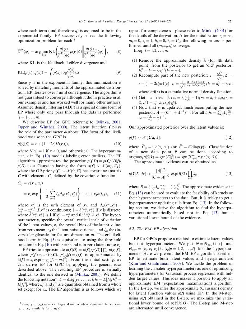
of preprocessing further cropped the face images to excludehair and background. Fig. 4 shows the example of a nor-malized image (256 · 256) and a cropped face image

H.-C. Kim et al. / Pattern Recognition Letters 27 (2006) 618–626 623

(28 · 23, cropped type A) and a more cropped face image(20 · 16, cropped type B). All images are aligned so thateyes are placed in the same positions, which can be done

0

0.05

0.1

0.15

0.2

0.25

0.3

Methods

Err

or r

ates

1-NN LDA SVM-CV SVM-EP GPC-EP

0

0.05

0.1

0.15

0.2

0.25

0.3

Methods

Err

or r

ates

1-NN LDA SVM-CV SVM-EP GPC-EP

(a) (

(c) (

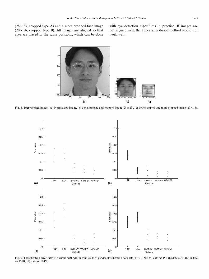
Fig. 5. Classification error rates of various methods for four kinds of gender clset P-III, (d) data set P-IV.

Fig. 4. Preprocessed images: (a) Normalized image, (b) downsampled and crop

with eye detection algorithms in practice. If images arenot aligned well, the appearance-based method would notwork well.

0

0.05

0.1

0.15

0.2

0.25

0.3

Methods

Err

or r

ates

1-NN LDA SVM-CV SVM-EP GPC-EP

0

0.05

0.1

0.15

0.2

0.25

0.3

Methods

Err

or r

ates

1-NN LDA SVM-CV SVM-EP GPC-EP

b)

d)

assification data sets (PF�01 DB): (a) data set P-I, (b) data set P-II, (c) data

ped image (28 · 23), (c) downsampled and more cropped image (20 · 16).

0

0.05

0.1

0.15

0.2

0.25

0.3

Methods

Err

or r

ates

1-NN LDA SVM-CV SVM-EP GPC-EP 0

0.05

0.1

0.15

0.2

0.25

0.3

Methods

Err

or r

ates

1-NN LDA SVM-CV SVM-EP GPC-EP

0

0.05

0.1

0.15

0.2

0.25

0.3

Methods

Err

or r

ates

1-NN LDA SVM-CV SVM-EP GPC-EP 0

0.05

0.1

0.15

0.2

0.25

0.3

Methods

Err

or r

ates

1-NN LDA SVM-CV SVM-EP GPC-EP

(a) (b)

(c) (d)

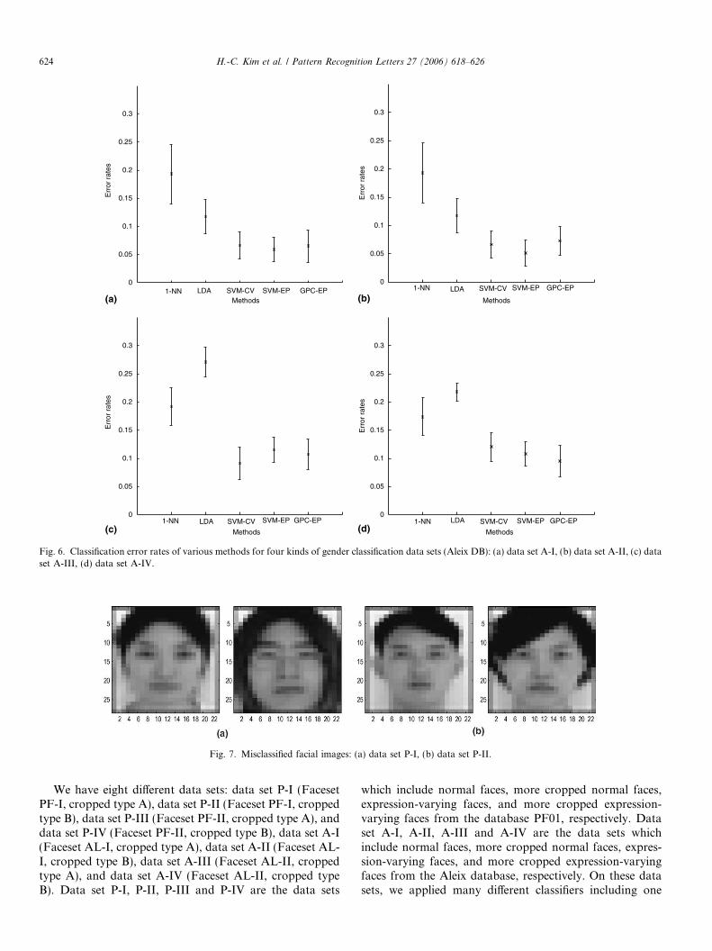
Fig. 6. Classification error rates of various methods for four kinds of gender classification data sets (Aleix DB): (a) data set A-I, (b) data set A-II, (c) dataset A-III, (d) data set A-IV.

Fig. 7. Misclassified facial images: (a) data set P-I, (b) data set P-II.

624 H.-C. Kim et al. / Pattern Recognition Letters 27 (2006) 618–626

We have eight different data sets: data set P-I (FacesetPF-I, cropped type A), data set P-II (Faceset PF-I, croppedtype B), data set P-III (Faceset PF-II, cropped type A), anddata set P-IV (Faceset PF-II, cropped type B), data set A-I(Faceset AL-I, cropped type A), data set A-II (Faceset AL-I, cropped type B), data set A-III (Faceset AL-II, croppedtype A), and data set A-IV (Faceset AL-II, cropped typeB). Data set P-I, P-II, P-III and P-IV are the data sets

which include normal faces, more cropped normal faces,expression-varying faces, and more cropped expression-varying faces from the database PF01, respectively. Dataset A-I, A-II, A-III and A-IV are the data sets whichinclude normal faces, more cropped normal faces, expres-sion-varying faces, and more cropped expression-varyingfaces from the Aleix database, respectively. On these datasets, we applied many different classifiers including one

H.-C. Kim et al. / Pattern Recognition Letters 27 (2006) 618–626 625

nearest neighbor (1-NN), linear discriminant analysis(LDA), SVM with cross-validation (SVM-CV), SVM withEM–EP hyperparameters (SVM-EP), and GPC with theEM–EP algorithm (GPC-EP). Figs. 5 and 6 show the clas-sification error rates of these methods over four differentdata sets in the database PF01 and Aleix database. Eachdata set was divided into 10 folds. Each fold was subse-quently used as a test set, while the other nine folds wereused as a training set. Before GPC or SVM are applied,all feature values are normalized based on the trainingset so that their means are zero and their variances areone. The points �·� in Figs. 5 and 6 are means of 10 trialsand error bars are from standard deviations of the meanestimators. In Fig. 7, we show misclassified images. InFig. 7(a), we can know that long hair is not always a keyfeature of women. The classification rates of data sets ofcropped type A are not always better than ones of croppedtype B.

GPC-EP used a single lengthscale hyperparameter (i.e.lm = l) for all feature dimensions4. In all GPC models thehyperparameter � was not updated but fixed to zero. InSVM-EP the kernel (i.e. covariance function) had the samehyperparameters as the corresponding GPC-EP that weretrained using EM–EP except for the latent noise variancev2 which was omitted because it caused degradation inSVM performance5. Instead, the penalty parameter C

allowing training errors (i.e. penalizing the SVM slack vari-ables) was selected by 5-fold cross-validation.6 In SVM-CVwe applied SVMs with a Gaussian kernel with a singlelengthscale hyperparameter (without v0, v1 and v2) selectedby five-fold cross-validation.7 We also had to determine thepenalty parameter C, so we performed a 2-level grid searchover a 2-dimensional parameter space (C, l)8.

In the data set P-I, P-II, P-IV, and A-IV, GPC-EP is thebest, in the data set P-III, A-I, and A-II, SVM-EP is thebest, and in the data set A-III SVM-CV is the best. In allthe data sets except for one, GPC-EP or SVM-EP is thebest. Also, in all the data sets except for one, SVM-EP isbetter than SVM-CV. Therefore, for the data sets testedthe hyperparameters found by the EM–EP algorithm seemto be also more suitable hyperparameters for SVMs thanthe ones obtained by cross-validation. This shows thatthe EM–EP algorithm finds suitable hyperparameters suc-cessfully and those hyperparameters are also suitable for

4 The initial values of hyperparameters for the first fold were as follows:v00 ¼ 1, v01 ¼ 0:0001, v02 ¼ 0:001, l0m ¼ l0 ¼ 1=ð2� dÞ; 8m, and those forsubsequent folds are the results for the former fold.5 For SVMs, we used the MATLAB Support Vector Machine Toolbox

available from http://theoval.sys.uea.ac.uk/~gcc/svm/tool-box with modified kernel functions.6 Firstly, we did a coarse grid search over fCjlog10C ¼ 0; 0:5; 1; 1:5;

2; 2:5; 3g to obtain C1. Then did a finer grid search over fCjlog10C ¼�0:4þ logC1;�0:3þ logC1; . . . ; 0:4þ logC1g.7 Similarly to the selection of C, we did a 2-level grid search over

fljlog10l ¼ �3;�2:5;�2;�1:5;�1;�0:5; 0g and fljlog10l ¼ �0:4þ log10l1;�0:3þ log l1; . . . ; 0:4þ log l1g.8 The same grids as above for parameters C, l were used.

SVMs. This result is consistent with the result on thebenchmark data sets in (Kim and Ghahramani, 2003).

6. Conclusion

We have proposed the appearance-based gender classifi-cation method with Gaussian processes. GPCs incorporatethe Bayesian model selection framework to determine thekernel hyperparameters, which is an important advantageover SVMs. In the experiments the hyperparametersobtained by GPC with the EM–EP algorithm were evenmore suitable for SVMs than the ones obtained by cross-validation. In most of the data sets, EM–EP algorithmsworked better than SVMs with cross-validation andprovided kernel hyperparameters to make SVMs workbetter.

We used Gaussian kernels in this paper. Gaussian ker-nels do not seem to be ideal for image data since they donot capture correlations between pixels. If we invent moreproper kernels for face images, we might improve the per-formance. It would also be interesting to perform experi-ments on a larger face data set.

Acknowledgments

Hyun-Chul Kim, Daijin Kim and Sung-Yang Bangwould like to thank the Ministry of Education of Koreafor its financial support toward the Division of Mechanicaland Industrial Engineering, and the Division of Electricaland Computer Engineering at POSTECH through BK21program.

References

Brunelli, R., Poggio, T., 1992. Hyperbf networks for gender classification.In: DARPA Image Understanding Workshop.

Burton, A., Bruce, V., Dench, N., 1993. What�s the difference between menand women? Evidence from facial measurements. Perception 22, 153–176.

Costen, N., Brown, M., Akamatsu, S., 2004. Sparse models for genderclassification. In: Proceedings of the 6th International Conference onAutomatic Face and Gesture Recognition.

Cottrell, G., Metcalfe, J., 1991. EMPATH: Face, emotion, and genderrecognition using holonsAdvances in Neural Information ProcessingSystems 3, vol. 3. MIT Press.

Gibbs, M., MacKay, D.J.C., 2000. Variational Gaussian process classi-fiers. IEEE Trans. NN 11 (6), 1458.

Golomb, B., Lawrence, D., Sejnowski, T., 1991. SEXNET: A neuralnetwork identifies sex from human faces. In: Advances in neuralinformation processing systems 3, vol. 3. MIT Press.

Gutta, S., Huang, J.R.J., Jonathon, P., Wechsler, H., 2000. Mixture ofexperts for classification of gender, ethnic origin, and pose of humanfaces. IEEE Trans. Neural Networks 11 (4), 948–960.

Jain, A., Huang, J., 2004. Integrating independent components and lineardiscriminant analysis. In: Proceedings of the 6th International Con-ference on Automatic Face and Gesture Recognition.

Kim, H.-C., Ghahramani, Z., 2003. The EM–EP algorithm forGaussian process classification. In: Proceedings of the Workshop onProbabilistic Graphical Models for Classification (ECML), pp. 37–48.

626 H.-C. Kim et al. / Pattern Recognition Letters 27 (2006) 618–626

Kim, H.-C., Sung, J.-W., Je, H.-M., Kim, S.-K., Jun, B.-J., Kim, D.,Bang, S.-Y., 2001. Asian face image database PF01. Technical Report,Intelligent Multimedia Lab, Department of CSE, POSTECH.

Martinez, A., Benavente, R., 1998. The ar face database. CVC TechnicalReport #24.

Minka, T., 2001. A family of algorithms for approximate Bayesianinference. Ph.D. Thesis, MIT.

Moghaddam, B., Yang, M., 2002. Learning gender with support faces.IEEE Trans. Pattern Anal. Mach. Intell. 24 (5), 707–711.

Neal, R., 1997. Monte Carlo implementation of Gaussian process modelsfor Bayesian regression and classification. Technical Report CRG-TR-97-2, Department of Computer Science, University of Toronto.

O�Hagan, A., 1978. On curve fitting and optimal design for regression.J. Royal Stat. Soc. B 40, 1–32.

Opper, M., Winther, O., 2000. Gaussian processes for classification: Meanfield algorithms. Neural Comput. 12, 2655–2684.

Tamura, S., Kawai, Mitsumoto, H., 1996. Male/female identification from8 · 6 very low resolution face images by neural networks. PatternRecogn. 29 (2), 331–335.

Williams, C.K.I., Barber, D., 1998. Bayesian classification with Gaussianprocesses. IEEE Trans. PAMI 20, 1342–1351.

Williams, C.K.I., Rasmussen, C.E., 1995. Gaussian processes for regres-sion. In: NIPS 8, vol. 8. MIT Press.