Apolarity, Hessian and Macaulay polynomials · Apolarity, Hessian and Macaulay polynomials This...
13
•
Transcript of Apolarity, Hessian and Macaulay polynomials · Apolarity, Hessian and Macaulay polynomials This...
Loughborough UniversityInstitutional Repository
Apolarity, Hessian andMacaulay polynomials
This item was submitted to Loughborough University's Institutional Repositoryby the/an author.
Citation: DI BIAGIO, L. and POSTINGHEL, E., 2013. Apolarity, Hessianand Macaulay Polynomials. Communications in Algebra, 41(1), pp. 226-237.
Additional Information:
• This is an Accepted Manuscript of an article published by Taylor &Francis in Communications in Algebra on 04 Jan 2013, available online:http://dx.doi.org/10.1080/00927872.2011.629265
Metadata Record: https://dspace.lboro.ac.uk/2134/25239
Version: Accepted for publication
Publisher: c© Taylor & Francis
Rights: This work is made available according to the conditions of the Cre-ative Commons Attribution-NonCommercial-NoDerivatives 4.0 International(CC BY-NC-ND 4.0) licence. Full details of this licence are available at:https://creativecommons.org/licenses/by-nc-nd/4.0/
Please cite the published version.
APOLARITY, HESSIAN AND MACAULAY POLYNOMIALS
LORENZO DI BIAGIO AND ELISA POSTINGHEL
Abstract. A result by Macaulay states that an Artinian graded Goren-stein ring R of socle dimension one and socle degree δ can be realizedas the apolar ring C[ ∂
∂x0, . . . , ∂
∂xn]/g⊥ of a homogeneous polynomial g
of degree δ in x0, . . . , xn. If R is the Jacobian ring of a smooth hyper-surface f(x0, . . . , xn) = 0 then δ is equal to the degree of the Hessianpolynomial of f . In this paper we investigate the relationship between gand the Hessian polynomial of f and we provide a complete descriptionfor n = 1 and deg(f) ≤ 4 and for n = 2 and deg(f) ≤ 3.
1. Introduction: the problem
Let f ∈ R = C[x0, . . . , xn] be a homogeneous polynomial. The ideal J(f)generated by the partial derivatives of f is called the Jacobian ideal, or thegradient ideal, of f . In the smooth case this ideal contains a power of theirrelevant ideal, so it has maximum depth in the coordinates ring and itis generated by a regular sequence. The associated ring R(f) = R/J(f),the so-called Jacobian ring of f , is an Artinian Gorenstein graded ring.Formal definitions can be found in Section 3. Both the Jacobian ideal and itscounterpart, the Jacobian ring, have been largely studied and it is now clear,form the work of P. Griffiths, that they reflect many geometric propertiesof the variety. For example if f and f ′ define smooth hypersurfaces then fand f ′ are projectively equivalent if and only if R(f) is isomorphic to R(f ′)thus allowing us to recover V (f) from its jacobian ring. Moreover partialinformation about R(f) is equivalent to information about the Hodge groupsthat appear in the Hodge decomposition of Hn−1(V (f),C). See [4, §2] fora nice account on this stuff and further references. Neverthless so far theJacobian ring has not been completely understood.
Apolarity allows us to associate an Artinian Gorenstein graded ring to aform. This nice property is described in a classical theorem due to Macaulay(Theorem 2.2): there exists a homogeneous polynomial (the Macaulay poly-nomial) g such that J(f) is equal to g⊥, where g⊥ ⊂ T = C[ ∂
∂x0, . . . , ∂
∂xn]
(upon identifying xi with ∂∂xi
). Apolarity is a very good tool to study vari-
eties of sum of powers (see for example [10, 11, 13]), which are the objectsof a very deep and challenging research area in Algebraic Geometry.
It is not so immediate to compute by hand the Macaulay polynomialassociated to a given Artinian Gorenstein graded ring, but in the case of theJacobian ring it seems natural to look at the Hessian polynomial Hess(f)of f since it has the right degree. It immediately turns out that if f is a
2000 Mathematics Subject Classification. Primary 14N15; Secondary 14J70.Key words and phrases. Apolarity, Macaulay correspondence, Jacobian ring, Hessian
polynomial.
1
2 LORENZO DI BIAGIO AND ELISA POSTINGHEL
Fermat polynomial, then Hess(f) and the Macaulay polynomial associatedto R(f) coincide, up to scalars (see Example 3.1). Therefore we ask ourselvesif Hess(f) is always the Macaulay polynomial (up to scalar multiplication)associated to f . A first naive conjecture is the following: J(f) = Hess(f)⊥,for every smooth homogeneous polynomial f ∈ R.
We will see in Section 3 that the question is not actually meaningful,anyway the answer is ‘no’ in general, but ‘yes’ in certain cases.
In Section 4 we will study the question for binary forms, giving a completeanswer for forms of degree 3 and 4.
In Section 5 we will completely answer the question in the plane cubicscase.
In Section 6 we will present a first attempt to study plane quartics, givingsome specific examples.
In Section 7 we will see how to use the computer algebra system CoCoAto attack this problem.
2. Preliminaries
We work over the complex numbers C, but all the results hold for anyalgebraically closed field of characteristic zero. Let S := C[x0, . . . , xn] bethe polynomial ring in n + 1 variables, let T := C[∂0, . . . , ∂n] be the C-algebra generated by the partial derivatives ∂i, where ∂i := ∂
∂xi. S and T
are naturally graded rings and we denote by Sd and Td their degree d part,which is of course a C-vector space of dimension
(n+dd
).
By the natural differentiation action of T on S we can view S as a T -module. Analogously we can think of S as the algebra of partial derivativeson T , hence we can also view T as an S-module. These two actions definea perfect pairing between homogeneous forms of degree j (cf. [8, Prop. 2.3]or [9]):
(1) Sj × Tj → C.
Given g ∈ S and f ∈ T we will say that f is apolar to g if f · g = 0.
Remark 2.1. If f, g are homogeneous of the same degree then g · f = f · g.
Regarding S as a (left) T -module, let I ⊆ T be an ideal and let M,P ⊆ Sbe T -submodules of S. Recall that (P :I M) := {i ∈ I|iM ⊆ P} is anideal of T contained in I. If M is principal, M = Tg, then we will write(P :I g) instead of (P :I M). Analogously, if M ⊆ P , then recall that(M :P I) := {p ∈ P |ip ∈M ∀i ∈ I} is a T -submodule of P .
In particular for any polynomial g ∈ S \ {0} we will denote by g⊥ theideal of T of forms apolar to g, i.e. g⊥ := Ann(g) = {f ∈ T |f · g = 0} =
(0 :T g). Let Tg := T/g⊥; since√g⊥ = (∂0, . . . , ∂n) then Tg is an Artinian
(0-dimensional) local ring.Recall that a zero-dimensional local ring A is Gorenstein if and only if
its socle (i.e. the annihilator of the unique maximal ideal) is simple (cf. [7,Prop. 21.5]). If moreover the ring is graded, we will call socle degree themaximum integer j such that Aj 6= 0. Recall the following theorem (see [7,theorem 21.6], [12, §60ff], [9, lemma 2.12] or the lecture notes by Geramita,esp. lecture 8 in [8]):
APOLARITY, HESSIAN AND MACAULAY POLYNOMIALS 3
Theorem 2.2 (Macaulay). With notation as above, there is a one-to-oneinclusion reversing correspondence between finitely generated nonzero T -submodules M ⊆ S and ideals I ⊆ T such that I ⊆ (∂0, . . . , ∂n) and T/I isa local Artinian ring, given by
M 7→ (0 :T M), the annihilator of M in T ;
I 7→ (0 :S I), the submodule of S annihilated by I.
In particular, ideals I as above such that T/I is local Artinian Gorensteincorrespond to principal submodules Tg for some element g ∈ S \ {0} (i.e.I = g⊥).
Corollary 2.3 (Macaulay). The homogeneous ideals I as in Theorem 2.2such that T/I is graded local Artinian Gorenstein and of socle degree j cor-respond to principal submodules Tg, where g is a homogeneous polynomialin Sj.
Definition 2.4. We will call Macaulay polynomial associated to T/I thepolynomial g associated to T/I (up to scalar multiplication) as in Corollary2.3.
Remark 2.5. Some authors refer to the Macaulay polynomial as the dualsocle generator of T/I.
Remark 2.6. If g is a homogeneous polynomial of degree j, then the Hilbertfunction h(Tg) is symmetric with respect to j/2 (cf. [9, p. 9]). Hence byCorollary 2.3, if I ⊆ (∂0, . . . , ∂n) is a homogeneous ideal of T and T/I is(graded) local Artinian Gorenstein and of socle degree j, then its Hilbertfunction h(T/I) is symmetric with respect to j/2.
Given I ⊆ (∂0, . . . , ∂n) homogeneous ideal such that T/I is local ArtinianGorenstein and of socle degree j, one can wonder if there is a simple way todetermine the associated Macaulay polynomial g ∈ Sj . In fact the followingholds:
Remark 2.7. The Macaulay polynomial associated to T/I is any nonzeroelement of (0 :Sj Ij).
Proof. By Corollary 2.3, we know that (0 :S I) is a principal T -submodulegenerated by g, hence
(0 :S I) = Tg = T0g ⊕ . . .⊕ Tjg = (0 :Sj I)⊕ · · · ⊕ (0 :S0 I),
and T0g = Cg, the C-vector space of dimension 1 generated by g. Thereforeany nonzero element of T0g = (0 :Sj I) = {s ∈ Sj |is = 0 ∀i ∈ I} can bechosen as g. Moreover since T/I has socle degree j and socle dimension1, then Ij is a C-vector subspace of Tj of codimension 1, hence, by (1),(0 :Sj Ij) has dimension 1. Since (0 :Sj Ij) ⊇ (0 :Sj I) and they have thesame dimension we have that (0 :Sj Ij) = (0 :Sj I). �
3. Jacobian ring and Hessian polynomial
Set R := C[x0, . . . , xn]. Let Rd be its homogeneous degree d part. ClearlyR = S, but when we write R instead of S we stress the fact that we viewthe polynomial ring as the C-algebra of partial derivatives, by the action
4 LORENZO DI BIAGIO AND ELISA POSTINGHEL
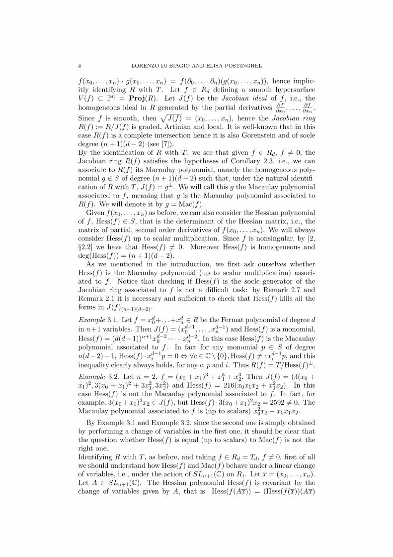
f(x0, . . . , xn) · g(x0, . . . , xn) = f(∂0, . . . , ∂n)(g(x0, . . . , xn)), hence implic-itly identifying R with T . Let f ∈ Rd defining a smooth hypersurfaceV (f) ⊂ Pn = Proj(R). Let J(f) be the Jacobian ideal of f , i.e., the
homogeneous ideal in R generated by the partial derivatives ∂f∂x0
, . . . , ∂f∂xn .
Since f is smooth, then√J(f) = (x0, . . . , xn), hence the Jacobian ring
R(f) := R/J(f) is graded, Artinian and local. It is well-known that in thiscase R(f) is a complete intersection hence it is also Gorenstein and of socledegree (n+ 1)(d− 2) (see [7]).By the identification of R with T , we see that given f ∈ Rd, f 6= 0, theJacobian ring R(f) satisfies the hypotheses of Corollary 2.3, i.e., we canassociate to R(f) its Macaulay polynomial, namely the homogeneous poly-nomial g ∈ S of degree (n+ 1)(d− 2) such that, under the natural identifi-cation of R with T , J(f) = g⊥. We will call this g the Macaulay polynomialassociated to f , meaning that g is the Macaulay polynomial associated toR(f). We will denote it by g = Mac(f).
Given f(x0, . . . , xn) as before, we can also consider the Hessian polynomialof f , Hess(f) ∈ S, that is the determinant of the Hessian matrix, i.e., thematrix of partial, second order derivatives of f(x0, . . . , xn). We will alwaysconsider Hess(f) up to scalar multiplication. Since f is nonsingular, by [2,§2.2] we have that Hess(f) 6= 0. Moreover Hess(f) is homogeneous anddeg(Hess(f)) = (n+ 1)(d− 2).
As we mentioned in the introduction, we first ask ourselves whetherHess(f) is the Macaulay polynomial (up to scalar multiplication) associ-ated to f . Notice that checking if Hess(f) is the socle generator of theJacobian ring associated to f is not a difficult task: by Remark 2.7 andRemark 2.1 it is necessary and sufficient to check that Hess(f) kills all theforms in J(f)(n+1)(d−2).
Example 3.1. Let f = xd0+. . .+xdn ∈ R be the Fermat polynomial of degree d
in n+1 variables. Then J(f) = (xd−10 , . . . , xd−1n ) and Hess(f) is a monomial,
Hess(f) = (d(d−1))n+1xd−20 · · · · ·xd−2n . In this case Hess(f) is the Macaulaypolynomial associated to f . In fact for any monomial p ∈ S of degreen(d−2)−1, Hess(f) ·xd−1i p = 0⇔ ∀c ∈ C\{0},Hess(f) 6= cxd−1i p, and this
inequality clearly always holds, for any c, p and i. Thus R(f) = T/Hess(f)⊥.
Example 3.2. Let n = 2, f = (x0 + x1)3 + x31 + x32. Then J(f) = (3(x0 +
x1)2, 3(x0 + x1)
2 + 3x21, 3x22) and Hess(f) = 216(x0x1x2 + x21x2). In this
case Hess(f) is not the Macaulay polynomial associated to f . In fact, forexample, 3(x0 +x1)
2x2 ∈ J(f), but Hess(f) ·3(x0 +x1)2x2 = 2592 6= 0. The
Macaulay polynomial associated to f is (up to scalars) x20x2 − x0x1x2.By Example 3.1 and Example 3.2, since the second one is simply obtained
by performing a change of variables in the first one, it should be clear thatthe question whether Hess(f) is equal (up to scalars) to Mac(f) is not theright one.Identifying R with T , as before, and taking f ∈ Rd = Td, f 6= 0, first of allwe should understand how Hess(f) and Mac(f) behave under a linear changeof variables, i.e., under the action of SLn+1(C) on R1. Let x = (x0, . . . , xn).Let A ∈ SLn+1(C). The Hessian polynomial Hess(f) is covariant by thechange of variables given by A, that is: Hess(f(Ax)) = (Hess(f(x))(Ax)
APOLARITY, HESSIAN AND MACAULAY POLYNOMIALS 5
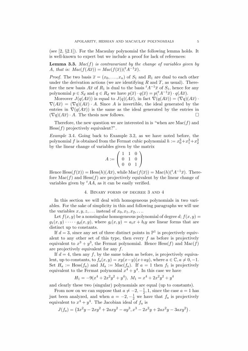
(see [2, §2.1]). For the Macaulay polynomial the following lemma holds. Itis well-known to expert but we include a proof for lack of references:
Lemma 3.3. Mac(f) is contravariant by the change of variables given byA, that is: Mac(f(Ax)) = Mac(f(x))(tA−1x).
Proof. The two basis x = (x0, . . . , xn) of S1 and R1 are dual to each otherunder the derivation actions (we are identifying R and T , as usual). There-fore the new basis Ax of R1 is dual to the basis tA−1x of S1, hence for anypolynomial p ∈ Sd and q ∈ Rd we have p(x) · q(x) = p(tA−1x) · q(Ax).
Moreover J(q(Ax)) is equal to J(q)(Ax), in fact ∇(q(Ax)) = (∇q)(Ax) ·∇(Ax) = (∇q)(Ax) · A. Since A is invertible, the ideal generated by theentries in ∇(q(Ax)) is the same as the ideal generated by the entries in(∇q)(Ax) ·A. The thesis now follows. �
Therefore, the new question we are interested in is “when are Mac(f) andHess(f) projectively equivalent?”.
Example 3.4. Going back to Example 3.2, as we have noted before, thepolynomial f is obtained from the Fermat cubic polynomial h := x30+x31+x32by the linear change of variables given by the matrix
A :=
1 1 00 1 00 0 1
Hence Hess(f(x)) = Hess(h)(Ax), while Mac(f(x)) = Mac(h)(tA−1x). There-fore Mac(f) and Hess(f) are projectively equivalent by the linear change ofvariables given by tAA, as it can be easily verified.
4. Binary forms of degree 3 and 4
In this section we will deal with homogeneous polynomials in two vari-ables. For the sake of simplicity in this and following paragraphs we will usethe variables x, y, z, . . . instead of x0, x1, x2, . . ..
Let f(x, y) be a nonsingular homogeneous polynomial of degree d; f(x, y) =g1(x, y) · · · · · gd(x, y), where gi(x, y) = aix + biy are linear forms that aredistinct up to constants.
If d = 3, since any set of three distinct points in P1 is projectively equiv-alent to any other set of this type, then every f as before is projectivelyequivalent to x3 + y3, the Fermat polynomial. Hence Hess(f) and Mac(f)are projectively equivalent for any f .
If d = 4, then any f , by the same token as before, is projectively equiva-lent, up to constants, to fa(x, y) = xy(x−y)(x+ay), where a ∈ C, a 6= 0,−1.Set Ha := Hess(fa) and Ma := Mac(fa). If a = 1 then f1 is projectivelyequivalent to the Fermat polynomial x4 + y4. In this case we have
H1 = −9(x4 + 2x2y2 + y4), M1 = x4 + 2x2y2 + y4
and clearly these two (singular) polynomials are equal (up to constants).From now on we can suppose that a 6= −2,−1
2 , 1, since the case a = 1 has
just been analyzed, and when a = −2,−12 we have that fa is projectively
equivalent to x4 + y4. The Jacobian ideal of fa is
J(fa) =(3x2y − 2xy2 + 2axy2 − ay3, x3 − 2x2y + 2ax2y − 3axy2
).
6 LORENZO DI BIAGIO AND ELISA POSTINGHEL
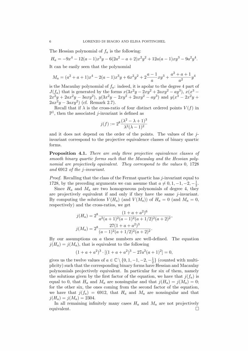
The Hessian polynomial of fa is the following:
Ha = −9x4 − 12(a− 1)x3y − 6(2a2 − a+ 2)x2y2 + 12a(a− 1)xy3 − 9a2y4.
It can be easily seen that the polynomial
Ma = (a2 + a+ 1)x4 − 2(a− 1)x3y + 6x2y2 + 2a− 1
axy3 +
a2 + a+ 1
a2y4
is the Macaulay polynomial of fa: indeed, it is apolar to the degree 4 part ofJ(fa) that is generated by the forms x(3x2y − 2xy2 + 2axy2 − ay3), x(x3 −2x2y + 2ax2y − 3axy2), y(3x2y − 2xy2 + 2axy2 − ay3) and y(x3 − 2x2y +2ax2y − 3axy2) (cf. Remark 2.7).
Recall that if λ is the cross-ratio of four distinct ordered points V (f) inP1, then the associated j-invariant is defined as
j(f) := 28(λ2 − λ+ 1)3
λ2(λ− 1)2
and it does not depend on the order of the points. The values of the j-invariant correspond to the projective equivalence classes of binary quarticforms.
Proposition 4.1. There are only three projective equivalence classes ofsmooth binary quartic forms such that the Macaulay and the Hessian poly-nomial are projectively equivalent. They correspond to the values 0, 1728and 6912 of the j-invariant.
Proof. Recalling that the class of the Fermat quartic has j-invariant equal to1728, by the preceding arguments we can assume that a 6= 0, 1,−1,−2,−1
2 .Since Ha and Ma are two homogeneous polynomials of degree 4, they
are projectively equivalent if and only if they have the same j-invariant.By computing the solutions V (Ha) (and V (Ma)) of Ha = 0 (and Ma = 0,respectively) and the cross-ratios, we get
j(Ha) = 28(1 + a+ a2)6
a2(a+ 1)2(a− 1)2(a+ 1/2)2(a+ 2)2,
j(Ma) = 2827(1 + a+ a2)3
(a− 1)2(a+ 1/2)2(a+ 2)2.
By our assumptions on a these numbers are well-defined. The equationj(Ha) = j(Ma), that is equivalent to the following
(1 + a+ a2)3 · [(1 + a+ a2)3 − 27a2(a+ 1)2] = 0,
gives us the twelve values of a ∈ C \ {0, 1,−1,−2,−12} (counted with multi-
plicity) such that the corresponding binary forms have Hessian and Macaulaypolynomials projectively equivalent. In particular for six of them, namelythe solutions given by the first factor of the equation, we have that j(fa) isequal to 0, that Ha and Ma are nonsingular and that j(Ha) = j(Ma) = 0;for the other six, the ones coming from the second factor of the equation,we have that j(fa) = 6912, that Ha and Ma are nonsingular and thatj(Ha) = j(Ma) = 2304.
In all remaining infinitely many cases Ha and Ma are not projectivelyequivalent. �
APOLARITY, HESSIAN AND MACAULAY POLYNOMIALS 7
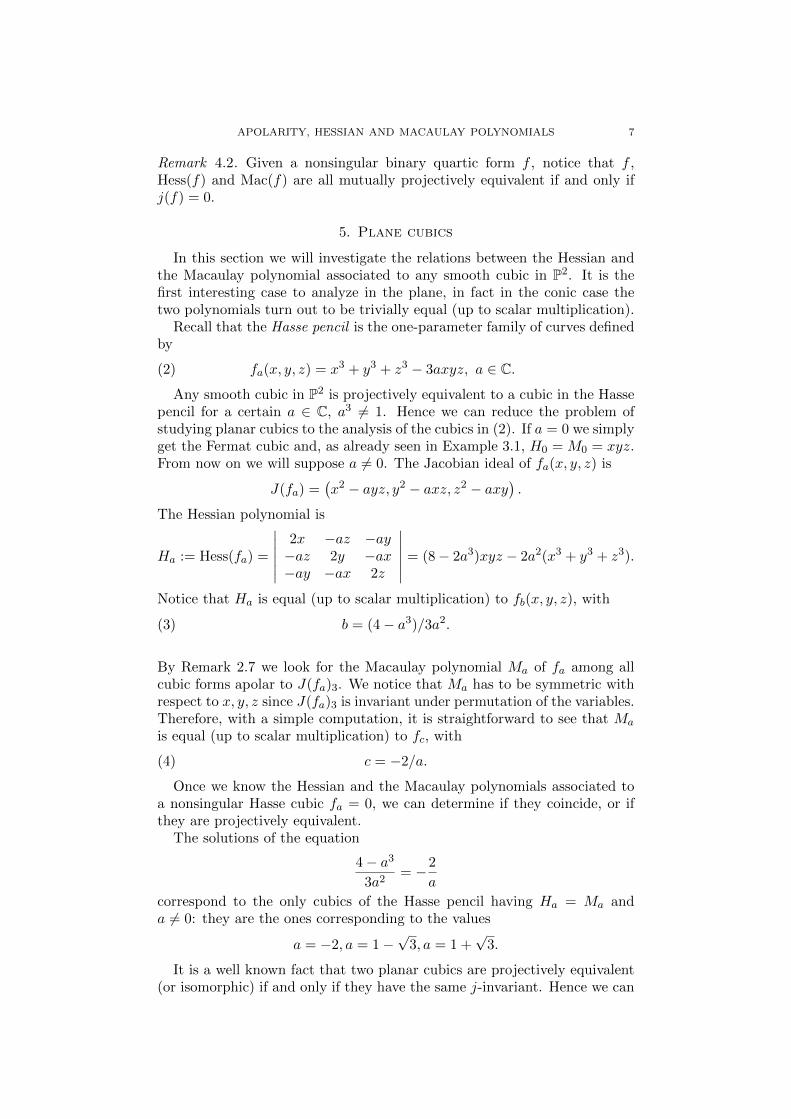
Remark 4.2. Given a nonsingular binary quartic form f , notice that f ,Hess(f) and Mac(f) are all mutually projectively equivalent if and only ifj(f) = 0.
5. Plane cubics
In this section we will investigate the relations between the Hessian andthe Macaulay polynomial associated to any smooth cubic in P2. It is thefirst interesting case to analyze in the plane, in fact in the conic case thetwo polynomials turn out to be trivially equal (up to scalar multiplication).
Recall that the Hasse pencil is the one-parameter family of curves definedby
fa(x, y, z) = x3 + y3 + z3 − 3axyz, a ∈ C.(2)
Any smooth cubic in P2 is projectively equivalent to a cubic in the Hassepencil for a certain a ∈ C, a3 6= 1. Hence we can reduce the problem ofstudying planar cubics to the analysis of the cubics in (2). If a = 0 we simplyget the Fermat cubic and, as already seen in Example 3.1, H0 = M0 = xyz.From now on we will suppose a 6= 0. The Jacobian ideal of fa(x, y, z) is
J(fa) =(x2 − ayz, y2 − axz, z2 − axy
).
The Hessian polynomial is
Ha := Hess(fa) =
∣∣∣∣∣∣2x −az −ay−az 2y −ax−ay −ax 2z
∣∣∣∣∣∣ = (8− 2a3)xyz − 2a2(x3 + y3 + z3).
Notice that Ha is equal (up to scalar multiplication) to fb(x, y, z), with
(3) b = (4− a3)/3a2.
By Remark 2.7 we look for the Macaulay polynomial Ma of fa among allcubic forms apolar to J(fa)3. We notice that Ma has to be symmetric withrespect to x, y, z since J(fa)3 is invariant under permutation of the variables.Therefore, with a simple computation, it is straightforward to see that Ma
is equal (up to scalar multiplication) to fc, with
(4) c = −2/a.
Once we know the Hessian and the Macaulay polynomials associated toa nonsingular Hasse cubic fa = 0, we can determine if they coincide, or ifthey are projectively equivalent.
The solutions of the equation
4− a3
3a2= −2
a
correspond to the only cubics of the Hasse pencil having Ha = Ma anda 6= 0: they are the ones corresponding to the values
a = −2, a = 1−√
3, a = 1 +√
3.
It is a well known fact that two planar cubics are projectively equivalent(or isomorphic) if and only if they have the same j-invariant. Hence we can
8 LORENZO DI BIAGIO AND ELISA POSTINGHEL
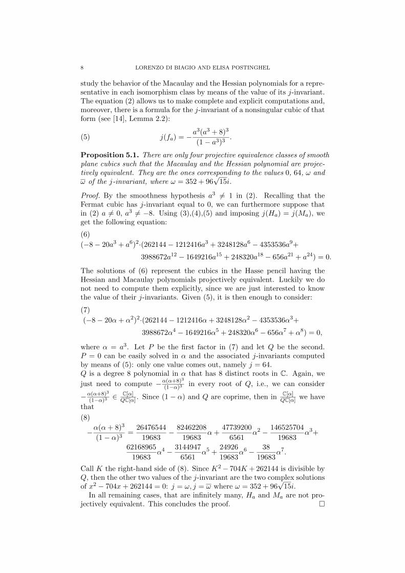
study the behavior of the Macaulay and the Hessian polynomials for a repre-sentative in each isomorphism class by means of the value of its j-invariant.The equation (2) allows us to make complete and explicit computations and,moreover, there is a formula for the j-invariant of a nonsingular cubic of thatform (see [14], Lemma 2.2):
j(fa) = −a3(a3 + 8)3
(1− a3)3.(5)
Proposition 5.1. There are only four projective equivalence classes of smoothplane cubics such that the Macaulay and the Hessian polynomial are projec-tively equivalent. They are the ones corresponding to the values 0, 64, ω andω of the j-invariant, where ω = 352 + 96
√15i.
Proof. By the smoothness hypothesis a3 6= 1 in (2). Recalling that theFermat cubic has j-invariant equal to 0, we can furthermore suppose thatin (2) a 6= 0, a3 6= −8. Using (3),(4),(5) and imposing j(Ha) = j(Ma), weget the following equation:
(−8− 20a3 + a6)2·(262144− 1212416a3 + 3248128a6 − 4353536a9+
(6)
3988672a12 − 1649216a15 + 248320a18 − 656a21 + a24) = 0.
The solutions of (6) represent the cubics in the Hasse pencil having theHessian and Macaulay polynomials projectively equivalent. Luckily we donot need to compute them explicitly, since we are just interested to knowthe value of their j-invariants. Given (5), it is then enough to consider:
(−8− 20α+ α2)2·(262144− 1212416α+ 3248128α2 − 4353536α3+
(7)
3988672α4 − 1649216α5 + 248320α6 − 656α7 + α8) = 0,
where α = a3. Let P be the first factor in (7) and let Q be the second.P = 0 can be easily solved in α and the associated j-invariants computedby means of (5): only one value comes out, namely j = 64.Q is a degree 8 polynomial in α that has 8 distinct roots in C. Again, we
just need to compute −α(α+8)3
(1−α)3 in every root of Q, i.e., we can consider
−α(α+8)3
(1−α)3 ∈C[α]QC[α] . Since (1− α) and Q are coprime, then in C[α]
QC[α] we have
that
−α(α+ 8)3
(1− α)3=
26476544
19683− 82462208
19683α+
47739200
6561α2 − 146525704
19683α3+
(8)
62168965
19683α4 − 3144947
6561α5 +
24926
19683α6 − 38
19683α7.
Call K the right-hand side of (8). Since K2− 704K + 262144 is divisible byQ, then the other two values of the j-invariant are the two complex solutionsof x2 − 704x+ 262144 = 0: j = ω, j = ω where ω = 352 + 96
√15i.
In all remaining cases, that are infinitely many, Ha and Ma are not pro-jectively equivalent. This concludes the proof. �
APOLARITY, HESSIAN AND MACAULAY POLYNOMIALS 9
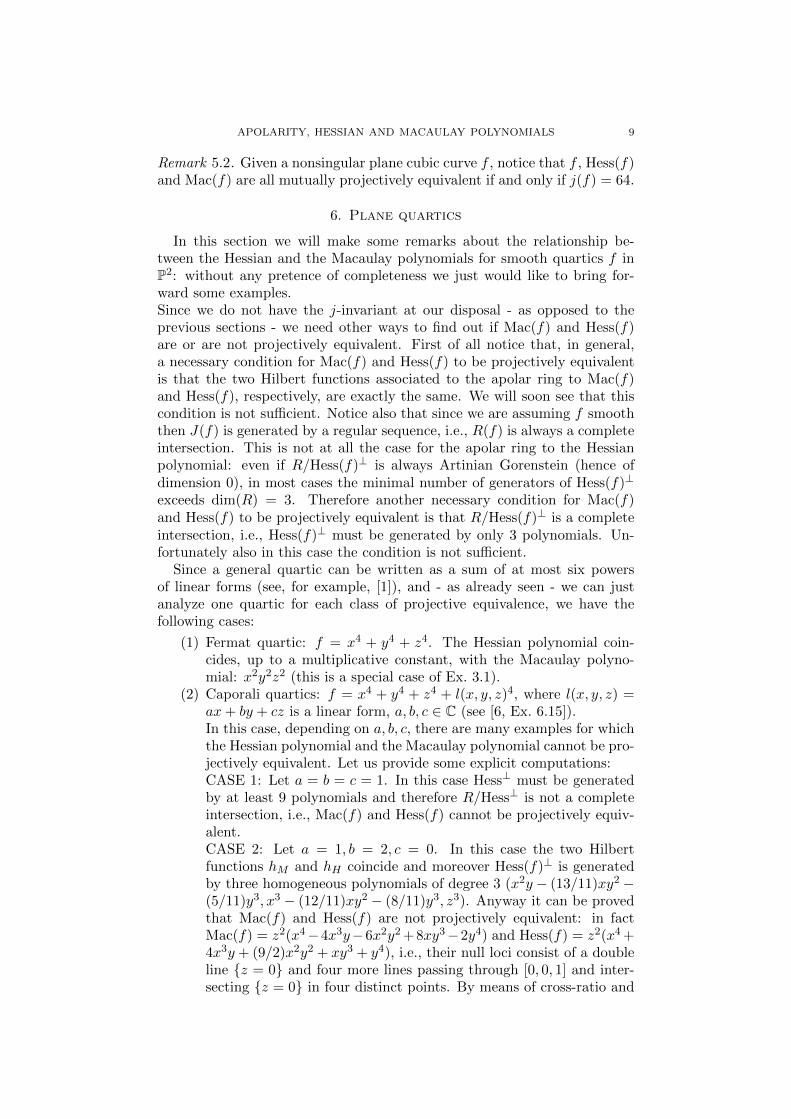
Remark 5.2. Given a nonsingular plane cubic curve f , notice that f , Hess(f)and Mac(f) are all mutually projectively equivalent if and only if j(f) = 64.
6. Plane quartics
In this section we will make some remarks about the relationship be-tween the Hessian and the Macaulay polynomials for smooth quartics f inP2: without any pretence of completeness we just would like to bring for-ward some examples.Since we do not have the j-invariant at our disposal - as opposed to theprevious sections - we need other ways to find out if Mac(f) and Hess(f)are or are not projectively equivalent. First of all notice that, in general,a necessary condition for Mac(f) and Hess(f) to be projectively equivalentis that the two Hilbert functions associated to the apolar ring to Mac(f)and Hess(f), respectively, are exactly the same. We will soon see that thiscondition is not sufficient. Notice also that since we are assuming f smooththen J(f) is generated by a regular sequence, i.e., R(f) is always a completeintersection. This is not at all the case for the apolar ring to the Hessianpolynomial: even if R/Hess(f)⊥ is always Artinian Gorenstein (hence ofdimension 0), in most cases the minimal number of generators of Hess(f)⊥
exceeds dim(R) = 3. Therefore another necessary condition for Mac(f)and Hess(f) to be projectively equivalent is that R/Hess(f)⊥ is a completeintersection, i.e., Hess(f)⊥ must be generated by only 3 polynomials. Un-fortunately also in this case the condition is not sufficient.
Since a general quartic can be written as a sum of at most six powersof linear forms (see, for example, [1]), and - as already seen - we can justanalyze one quartic for each class of projective equivalence, we have thefollowing cases:
(1) Fermat quartic: f = x4 + y4 + z4. The Hessian polynomial coin-cides, up to a multiplicative constant, with the Macaulay polyno-mial: x2y2z2 (this is a special case of Ex. 3.1).
(2) Caporali quartics: f = x4 + y4 + z4 + l(x, y, z)4, where l(x, y, z) =ax+ by + cz is a linear form, a, b, c ∈ C (see [6, Ex. 6.15]).In this case, depending on a, b, c, there are many examples for whichthe Hessian polynomial and the Macaulay polynomial cannot be pro-jectively equivalent. Let us provide some explicit computations:CASE 1: Let a = b = c = 1. In this case Hess⊥ must be generatedby at least 9 polynomials and therefore R/Hess⊥ is not a completeintersection, i.e., Mac(f) and Hess(f) cannot be projectively equiv-alent.CASE 2: Let a = 1, b = 2, c = 0. In this case the two Hilbertfunctions hM and hH coincide and moreover Hess(f)⊥ is generatedby three homogeneous polynomials of degree 3 (x2y − (13/11)xy2 −(5/11)y3, x3 − (12/11)xy2 − (8/11)y3, z3). Anyway it can be provedthat Mac(f) and Hess(f) are not projectively equivalent: in factMac(f) = z2(x4−4x3y−6x2y2 +8xy3−2y4) and Hess(f) = z2(x4 +4x3y + (9/2)x2y2 + xy3 + y4), i.e., their null loci consist of a doubleline {z = 0} and four more lines passing through [0, 0, 1] and inter-secting {z = 0} in four distinct points. By means of cross-ratio and
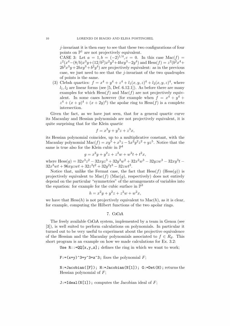
10 LORENZO DI BIAGIO AND ELISA POSTINGHEL
j-invariant it is then easy to see that these two configurations of fourpoints on P1 are not projectively equivalent.CASE 3: Let a = 1, b = (−2)1/4, c = 0. In this case Mac(f) =z2(x4−(8/b)x3y+(12/b2)x2y2+4bxy3−2y4) and Hess(f) = z2(b2x4+2b3x3y+2bxy3+b2y4) are projectively equivalent: as in the previouscase, we just need to see that the j-invariant of the two quadruplesof points is the same.
(3) Clebsh quartics: f = x4 + y4 + z4 + l1(x, y, z)4 + l2(x, y, z)
4, wherel1, l2 are linear forms (see [5, Def. 6.12.1]). As before there are manyexamples for which Hess(f) and Mac(f) are not projectively equiv-alent. In some cases however (for example when f = x4 + y4 +z4 + (x + y)4 + (x + 2y)4) the apolar ring to Hess(f) is a completeintersection.
Given the fact, as we have just seen, that for a general quartic curveits Macaulay and Hessian polynomials are not projectively equivalent, it isquite surprising that for the Klein quartic
f = x3y + y3z + z3x,
its Hessian polynomial coincides, up to a multiplicative constant, with theMacaulay polynomial Mac(f) = xy5 + x5z− 5x2y2z2 + yz5. Notice that thesame is true also for the Klein cubic in P4
g = x2y + y2z + z2w + w2t+ t2x,
where Hess(g) = 32x3z2 − 32xyz3 + 32y3w2 + 32x2w3 − 32yzw3 − 32xy3t−32x3wt+ 96xyzwt+ 32z3t2 + 32y2t3 − 32zwt3.
Notice that, unlike the Fermat case, the fact that Hess(f) (Hess(g)) isprojectively equivalent to Mac(f) (Mac(g), respectively) does not entirelydepend on the particular “symmetries” of the arrangements of variables intothe equation: for example for the cubic surface in P3
h = x2y + y2z + z2w + w2x,
we have that Hess(h) is not projectively equivalent to Mac(h), as it is clear,for example, computing the Hilbert functions of the two apolar rings.
7. CoCoA
The freely available CoCoA system, implemented by a team in Genoa (see[3]), is well suited to perform calculations on polynomials. In particular itturned out to be very useful to experiment about the projective equivalenceof the Hessian and the Macaulay polynomials associated to f ∈ Rd. Thisshort program is an example on how we made calculations for Ex. 3.2:
Use R::=QQ[x,y,z]; defines the ring in which we want to work;
F:=(x+y)^3+y^3+z^3; fixes the polynomial F ;
N:=Jacobian([F]); H:=Jacobian(N[1]); G:=Det(H); returns theHessian polynomial of F ;
J:=Ideal(N[1]); computes the Jacobian ideal of F ;
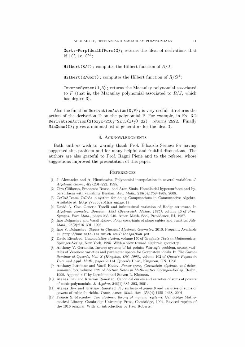
APOLARITY, HESSIAN AND MACAULAY POLYNOMIALS 11
Gort:=PerpIdealOfForm(G); returns the ideal of derivations thatkill G, i.e. G⊥;
Hilbert(R/J); computes the Hilbert function of R/J ;
Hilbert(R/Gort); computes the Hilbert function of R/G⊥;
InverseSystem(J,3); returns the Macaulay polynomial associatedto F (that is, the Macaulay polynomial associated to R/J , whichhas degree 3).
Also the function DerivationAction(D,P); is very useful: it returns theaction of the derivation D on the polynomial P. For example, in Ex. 3.2DerivationAction(216xyz+216y^2z,3(x+y)^2z); returns 2592. FinallyMinGens(I); gives a minimal list of generators for the ideal I.
8. Acknowledgments
Both authors wish to warmly thank Prof. Edoardo Sernesi for havingsuggested this problem and for many helpful and fruitful discussions. Theauthors are also grateful to Prof. Ragni Piene and to the referee, whosesuggestions improved the presentation of this paper.
References
[1] J. Alexander and A. Hirschowitz. Polynomial interpolation in several variables. J.Algebraic Geom., 4(2):201–222, 1995.
[2] Ciro Ciliberto, Francesco Russo, and Aron Simis. Homaloidal hypersurfaces and hy-persurfaces with vanishing Hessian. Adv. Math., 218(6):1759–1805, 2008.
[3] CoCoATeam. CoCoA: a system for doing Computations in Commutative Algebra.Available at http://cocoa.dima.unige.it.
[4] David A. Cox. Generic Torelli and infinitesimal variation of Hodge structure. InAlgebraic geometry, Bowdoin, 1985 (Brunswick, Maine, 1985), volume 46 of Proc.Sympos. Pure Math., pages 235–246. Amer. Math. Soc., Providence, RI, 1987.
[5] Igor Dolgachev and Vassil Kanev. Polar covariants of plane cubics and quartics. Adv.Math., 98(2):216–301, 1993.
[6] Igor V. Dolgachev. Topics in Classical Algebraic Geometry. 2010. Preprint. Availableat http://www.math.lsa.umich.edu/~idolga/CAG.pdf.
[7] David Eisenbud. Commutative algebra, volume 150 of Graduate Texts in Mathematics.Springer-Verlag, New York, 1995. With a view toward algebraic geometry.
[8] Anthony V. Geramita. Inverse systems of fat points: Waring’s problem, secant vari-eties of Veronese varieties and parameter spaces for Gorenstein ideals. In The CurvesSeminar at Queen’s, Vol. X (Kingston, ON, 1995), volume 102 of Queen’s Papers inPure and Appl. Math., pages 2–114. Queen’s Univ., Kingston, ON, 1996.
[9] Anthony Iarrobino and Vassil Kanev. Power sums, Gorenstein algebras, and deter-minantal loci, volume 1721 of Lecture Notes in Mathematics. Springer-Verlag, Berlin,1999. Appendix C by Iarrobino and Steven L. Kleiman.
[10] Atanas Iliev and Kristian Ranestad. Canonical curves and varieties of sums of powersof cubic polynomials. J. Algebra, 246(1):385–393, 2001.
[11] Atanas Iliev and Kristian Ranestad. K3 surfaces of genus 8 and varieties of sums ofpowers of cubic fourfolds. Trans. Amer. Math. Soc., 353(4):1455–1468, 2001.
[12] Francis S. Macaulay. The algebraic theory of modular systems. Cambridge Mathe-matical Library. Cambridge University Press, Cambridge, 1994. Revised reprint ofthe 1916 original, With an introduction by Paul Roberts.
12 LORENZO DI BIAGIO AND ELISA POSTINGHEL
[13] Kristian Ranestad and Frank-Olaf Schreyer. Varieties of sums of powers. J. ReineAngew. Math., 525:147–181, 2000.
[14] Boris Reichstein and Zinovy Reichstein. Surfaces parameterizing Waring presenta-tions of smooth plane cubics. Michigan Math. J., 40(1):95–118, 1993.
Dipartimento di Matematica, Universita degli Studi “Roma Tre” - LargoSan Leonardo Murialdo 1, 00146, Roma, Italy
E-mail address, 1: [email protected]
E-mail address, 2: [email protected]
Centre of Mathematics for Applications, University of Oslo - P.O. Box1053 Blindern, N0-0316 Oslo, Norway
E-mail address, 1: [email protected]
E-mail address, 2: [email protected]