“The Fundamental Factors Affecting Corn Price from 1982 ... Fundamental Factors... · different...
23
“The Fundamental Factors Affecting Corn Price from 1982-2013” Erin Whittaker Senior Honor’s Thesis April 11, 2014 1
Transcript of “The Fundamental Factors Affecting Corn Price from 1982 ... Fundamental Factors... · different...

“The Fundamental Factors Affecting Corn Price from 1982-2013”
Erin Whittaker
Senior Honor’s Thesis
April 11, 2014
1

Introduction
Corn prices have not been stable from 2007 to 2012 and there are many
different situations and events that influence corn price. Through my research, I will
be exploring and explaining the fundamental reasons that corn prices have become
increasingly more volatile. The factors that will be explored are split into two
different categories: supply and demand. The influences that follow under supply
include planted acreage of corn, expected corn yield, weather, and the effects of
commodity programs. The factors under demand include the amount of corn
consumption, ethanol production, exchange rates which affect exports and imports,
global stocks, and incomes. Most importantly, I will be focusing on effects of
weather, ethanol production, planted acreage of corn and expected corn yield. I have
observed that corn prices have increased in the past decade and that corn
production and ethanol production have increased immensely as well. I am gong to
research if and how these two factors are correlated, I will do this by running
regressions with corn price data from 1982 to 2013. The current research that I will
update and build on are the fundamental factors that are causing corn prices to
increase, all though my main focus will be the effect of ethanol production growth
on corn prices. The Congressional Budget Office clearly links the increase in corn
prices to domestic ethanol demand:
“In 2008, nearly 3 billion bushels of corn were used to produce ethanol in the United States. That amount constituted an increase over the previous year of almost a billion bushels. The demand for corn for ethanol production, along with other factors, exerted upward pressure on corn prices, which rose by more than 50 percent between April 2007 and April 2008.” Corn prices have become more volatile in the past decade and I will research how four
2

different factors have affected US corn price. These four variables are precipitation, US
Weighted Dollar Index, corn production, and ethanol price. I will run regressions, then
analyze the results and conclude which of these variables have significantly affected US
corn price.
Literature Review
Weather, ethanol, and planted corn acreage/expected corn yield are all fundamental
factors that are changing and impacting corn price. Wescott and Jewison (2012)
researched and compiled results about the impact that United States weather has had on
corn yields. They especially focused on the 2012 drought and its’ effects on corn
production, which were significantly lower in 2012 compared to past years. Abbott, Hurt,
and Tyner (2011) discuss corn production and the specific uses for corn and the effect of
different uses on corn prices. Ethanol is another significant influence on corn price.
According to Capehart and Vasadava (2012), ethanol’s effect on corn price is
approximately $0.41/bushel and they concluded that ethanol production has had a
positive impact on corn price. Gardebroek and Hernandez (2012) researched volatility
transmission in ethanol, oil, and corn prices between 1997 and 2011. They found
significant volatility spillovers from corn to ethanol but not from ethanol to corn. Another
factor is planted corn acreage and expected corn yield, which according to Wallandar,
Claassan, and Nickerson (2011) has increased along with corn prices increasing as well.
They state that corn production has not kept up with ethanol production growth, which
increases the demand for corn drastically. Condon, Klemick, and Wolverton (2013)
calculated the percentage effect of ethanol gallon expansion on corn prices. They found
that in the short run that there is a higher impact on corn prices per billion gallons of corn
3

ethanol production. They found that each billion gallons of ethanol would create a 5-10
percent increase in corn price (Condon, Klemick and Wolverton, 2013).
Weather
The last three years, 2012-2014, of United States weather has significantly
impacted corn prices. For instance, there was the 2012 drought, which included high
temperatures and extended periods with out rain. The drought affected many growing and
production regions in the United States. The impact was unfavorable and there was a
reduction of corn yields in 2012 to 123.4 bushels per acre. For three years national
average corn yields were reduced below trend expectations due to weather (Wescott and
Jewison, 2012). Figure 1 displays the predicted corn yield (bushels per acre) each year
along with the actual corn yield (bushels per acre) each year (Wescott and Jewison,
2012). Figure 1.0 includes data from 1988 through 2012, which includes both major
United States droughts.
Figure 1.0 Predicted and Actual US Corn Yield
4

Sources: Adapted from “Weather Effects on Expected Corn and Soybean Yields,” by Paul C. Westcott and Michael Jewison, 2012 Ethanol
Capehart and Vasadava (2012) state that biofuel production will continue to
increase because of the Energy Independence and Security Act (EISA). EISA
mandates an increase in biofuel use from 9.0 billion gallons in 2008 to 36 billion
gallons in 2022. Capehart and Vasada (2012) used log-log models to calculate short-
run price elasticity and corn production. The focus of their work is the effect of each
of the following categories of corn demand on US corn price between 1995 and
2006. They figure out the effect by estimating five equations, one equation for each
of the following factors: corn supply, corn price, feed demand, export demand, and
food/alcohol/industrial demand. Capehart and Vasada (2012) find that increasing
demand for FAI (food, alcohol, and industrial demand) is more important in
explaining corn price changes than other use categories. The impact of FAI
consumption on corn price is the strongest, following that is export consumption,
and then feed consumption is last. They estimate that ethanol’s effect on corn price
is about $.41/bushel, this is calculated using data from 2006-2008 (Capehart and
Vasadava, 2012). While $.41 is an increase in price it is not close to actual price
appreciation so Capehart and Vasadava (2012) concluded that ethanol production
has had a significant and positive impact on corn price but it does not fully explain
the corn price increase in the year 2007/2008.
Gardeborek and Hernandez (2012) examined volatility transmissions in corn
prices, ethanol, and oil in the United States between 1997 and 2011. They formed a
Multivariable Generalized Autoregressive Conditional Heteroskedascity (MGARCH)
5

Model to observe and calculate the volatility transmissions. They also used the
MGARCH model to calculate the interdependence, the dynamics, and the cross-
dynamics of volatility between corn markets, ethanol, and oil. Gardebroek and
Hernandez (2012) also observed the relationship between energy and agricultural
markets. They used the BEKK (Baba, Engle, Kraft, and Kroner) model to examine
this relationship. This model characterizes the volatility transmission across
markets, it also accounts for own and cross volatility spillovers and persistence
between markets. They also used a DCC model to observe the change in level of
interdependence between markets across time. The DCC does this by approximating
the dynamic conditional correlation matrix. The results of these models and
calculations indicated a higher interaction between ethanol and corn markets
between 2006-2011. After 2006 Gardebroek and Hernandez (2012) found a higher
correlation between corn and ethanol markets, prior to 2006 they only observed a
strong correlation between oil and ethanol returns. The results also showed large
own-volatility effects in the three markets (crude oil, corn, and ethanol), which
indicate that there were strong Generalized Autoregressive Conditional
Heteroskedascity (GARCH) effects (Gardebroek and Hernandez, 2012). The ethanol
markets displayed the lowest own-volatility persistence (Gardebroek and
Hernandez, 2012).
Abbott, Hurt, and Tyner (2011) state that since the 2005/06 marketing year
88% of growth in total global corn use has been in the food, seed, and industrial
(FSI) category. Ethanol is placed in the FSI category. Since 2005/06 total corn used
specifically for ethanol has increased 2.46 billion bushels annually, as a result this
6

increase use of corn for ethanol in the US was 48% of the increase in corn utilization
globally over the next 5 years.
According to Condon, Klemick and Wolverton (2013) for each billion gallon
expansion in ethanol production there is a 5-10% increase in corn prices. Condon,
Klemick and Wolverton (2013) normalized corn price impacts by ethanol quantity to
calculate two metrics: percent change in corn prices per 1 billion gallon increase in
corn ethanol production and percent change in corn prices per 1% increase in corn
ethanol production. Condon, Klemick and Wolverton (2013) found that each billion
gallon expansion in corn ethanol production increase 2-3% ong run corn price.
From 2000-2012 US ethanol production has increased by more than 700% and that
the percent of US corn harvested used for ethanol has increased from 10% to 40%.
(Condon, Klemick and Wolverton, 2013)
Figure 2.0 Percent of Corn Production Used for Ethanol and Corn Prices
Sources: Capehart and Vasada Economic Research Services Feed Grain Database (2013b) Commented [ACE1]: Is this a document I can find, or did you use these data to create the figure?
7

Planted Acreage and Expected Yield
Wallander, Claassen, and Nickerson (2011) have found that corn production
has increased between 2000-2009 due to increased corn yields and that corn prices
increased dramatically between 2006 and 2008. At the same time between 2000
and 2009 US ethanol production has increased by 9.2 billion gallons, moving from
1.6 gallons in 2000 to 10.8 gallons being produced in 2009. During this time US corn
production increased a total of 3.2 million bushels and harvested corn increased a
total of 7.2 million acres. Corn prices are increasing because corn acreage and corn
yield expansion have not kept up with ethanol production growth (Claassen,
Nickerson, and Wallander, 2011). Wallander, Claassan, and Nickerson (2011) state
that agricultural markets can keep up with the growing demand for ethanol by
diverting corn from other uses, increasing corn yields, or increasing the amount of
land planted to corn. Through out the past decade all of these changes have
occurred and continue to change as ethanol production increases. Figure 3.0 shows
that the demand for corn used for corn-based ethanol is increasing rapidly.
Figure 3.0
8

US Uses for Corn (billion bushels)
Sources: ”The Ethanol Decade- An Expansion of US Corn Production, 2000-09” Wallander, Claassen, Nickerson (2011)
According to Abbot, Hurt, and Tyner (2011) in 2005 7.8 million acres of corn
was harvested specifically for ethanol. In 2010 23.7 million acres of corn was
harvested specifically for ethanol, this is an increase of 15.9 million acres between
2005 and 2010.
Abbott, Hurt, and Tyner (2011) state that due to the biofuel policy
constraints the demand for corn that is used for biofuel is fixed. For example, RFS 2
(Renewable Fuel Standard) mandates gasoline blenders use 15 billion gallons of
corn-based ethanol by 2015. In 2010, the US produced 13 billion gallons of ethanol
and in 2011 the US produced more than 14 billion gallons of ethanol. The US is
quickly approaching the RFS 2 mandate. This will cause growth in this sector of corn
production to slow exponentially.
Empirical Model
We wanted to see how precipitation, corn production, ethanol price, and the
US Weighted Dollar Index affected US corn price. Figure 4.0 displays the variation of
the four independent variables in relation to US corn price. . Since the data does not
9

have the same units we divided each of the data series by the first data point to
make all of the data points out of one. According to Figure 4.0, ethanol price has
increased steadily with a major spike around September of 2006. Corn production
has also increased fairly steadily with some drops and rises but over all it has
increased. This could be due to an increase in technology that has increased
production efficiency and capacity. Precipitation is the most volatile independent
variable, which one can expect due to the uncertainty of weather. And lastly, the US
Dollar Weight index increased towards the beginning but has remained pretty
steady with a slight decline towards the end.
Figure 4.0
Independent Variables vs. US Corn Price (1982-2013)
Sources: Erin Whittaker created with data used for the regression
0.00
0.50
1.00
1.50
2.00
2.50
Corn
Pr R
1.16
1.23
0.90
0.60
1.04
0.89
0.95
0.85
1.05
0.93
1.69
0.99
0.80
0.60
0.78
0.92
0.92
0.76
1.33
2.07
1.42
2.50
3.00
Inde
pend
ent V
aria
bles
(Var
ying
Uni
ts)
Corn Price (1982-2013)
Independent Variables vs. Corn Price (Dependent Variable)
#REF!
#REF!
#REF!
#REF!
10

We ran a linear regression to test whether United States average
precipitation, ethanol price, corn production, and the United States Dollar Index
significantly impacted corn price. Corn price was the dependent variable in our
regression and precipitation, ethanol price, corn production, and the United States
Dollar Index were the independent variables. The first regression we ran was the
base regression.
The left-hand side, , is the dependent variable, monthly United States
corn price. All of the variables on the right-hand side are independent variables
meaning that they are the inputs that are tested to see whether or not they affect the
dependent variable. The right-hand side includes, , the coefficient and/or
intercept. is the independent precipitation variable with a monthly subscript
of . Precipitation is the volume of precipitation in the United States. is the
independent weighted value of the US Dollar variable with a monthly subscript of .
is the United States corn production variable with a monthly subscript of .
is the independent variable for Omaha, Nebraska’s ethanol spot price with a
monthly subscript of . is the random error term/ residuals and are the lag
variables included (time minus number of lags which in our case is 1 to 12).
After running the first regression we tested for structural change to see if the
regression should be split into two different time periods. We split the regression
into two different time periods, 1982-2004 and 2004-2013. We selected this place
ytcp = βο + βpXtp + βwvXtwv + βcPtc + βeXte +ε +Yt − n
ytcp
βο
βpXtp
t
βwvXtwv
t
βcPtc
t
βeXte
t
ε
Yt − n
11

to split our data because it was when the Renewable Fuel Standard program was
created under the Energy Policy Act of 2005 which established the first renewable
fuel mandate in the US. We were interested in viewing how ethanol impacted corn
price.
Data and Methodology
Data
Corn price has been volatile and has increased drastically in the last five to
ten years as you can see in Figure 5.0.
Figure 5.0
US Corn Price 1982-2013
Sources: Created by Erin Whittaker, data from National Agricultural Statistics Service
0123456789
Dec-
77Se
p-79
Jun-
81M
ar-8
3De
c-84
Sep-
86Ju
n-88
Mar
-90
Dec-
91Se
p-93
Jun-
95M
ar-9
7De
c-98
Sep-
00Ju
n-02
Mar
-04
Dec-
05Se
p-07
Jun-
09
Pric
e ($
/bu)
Date
Corn Price
12
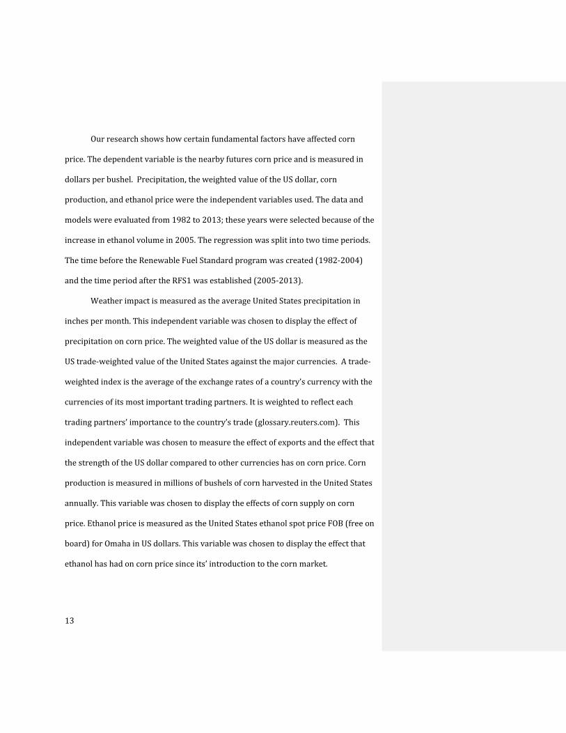
Our research shows how certain fundamental factors have affected corn
price. The dependent variable is the nearby futures corn price and is measured in
dollars per bushel. Precipitation, the weighted value of the US dollar, corn
production, and ethanol price were the independent variables used. The data and
models were evaluated from 1982 to 2013; these years were selected because of the
increase in ethanol volume in 2005. The regression was split into two time periods.
The time before the Renewable Fuel Standard program was created (1982-2004)
and the time period after the RFS1 was established (2005-2013).
Weather impact is measured as the average United States precipitation in
inches per month. This independent variable was chosen to display the effect of
precipitation on corn price. The weighted value of the US dollar is measured as the
US trade-weighted value of the United States against the major currencies. A trade-
weighted index is the average of the exchange rates of a country’s currency with the
currencies of its most important trading partners. It is weighted to reflect each
trading partners’ importance to the country’s trade (glossary.reuters.com). This
independent variable was chosen to measure the effect of exports and the effect that
the strength of the US dollar compared to other currencies has on corn price. Corn
production is measured in millions of bushels of corn harvested in the United States
annually. This variable was chosen to display the effects of corn supply on corn
price. Ethanol price is measured as the United States ethanol spot price FOB (free on
board) for Omaha in US dollars. This variable was chosen to display the effect that
ethanol has had on corn price since its’ introduction to the corn market.
13

Methodology
To begin analyzing the data we ran the Dickey-Fuller test on corn price to
test whether or not corn price was stationary. Since corn price is so volatile we ran
the Dickey-Fuller test with first differences. Our pt-1 (corn price with one lag)
coefficient was -3.04 so we rejected the null hypothesis meaning that with first
differences corn price is stationary. We also rejected the null hypothesis at the 5%
significance level. Once it was proven that the first differences were strongly
stationary, we ran a regression with the data from 1982-2013 to see which
independent variables were significant. After considering ethanol policy and
mandates we split the data into two different periods, one from 1982-2004 and the
second from 2005-2013. We decided to split the data in 2005 when the United
States became a large and influential producer of ethanol. The US Energy Policy Act
of 2005 mandated that gasoline contain 7.5 billion gallons of renewable fuel
annually by 2012. Since then that Act has been changed, in 2007 the RFS required 9
billion gallons of renewable fuels in 2008 and required that to increase to 15.2
billion gallons in 2012 and to 36 billion gallons in 2022 (Energy Policy Act of 2005).
Results
Before running the regression and obtaining the results we hypothesized
what we expected the signs on the coefficients for each independent variable. We
expected the US Weighted Dollar Index to have a negative coefficient. This is
because as the US dollar becomes weaker, other countries want to buy more US corn
because it is cheaper. The US ends up exporting more corn which lowers the supply
14

of corn in the US market which causes US corn price to increase. We expected US
precipitation to have a negative coefficient as well because if there is a decrease in
precipitation then there will be a decrease in harvest size. This will cause a decrease
in US corn supply and raise the US corn price. We expected corn production to also
have a negative coefficient because as corn production decreases, the US corn
supply decreases, and US corn price rises. We expected US ethanol spot price to
have a positive coefficient. We assumed that as US ethanol spot price rises then US
corn price should increase as well.
Figure 6.0
Regression Results
Variables Jan82-Sep13 Jan82-Dec04 Jan05-Sep13 Dollweight
-0.0011279 * (0.0007579)
-0.0008187 * (0.0005088)
-0.009141 ** (0.0045124)
Precip
-0.0389235 *** (0.0157752)
-0.0218294 ** (0.0116739)
-0.0565015 (0.0517999)
Cornprod
-0.0056663 (0.0051846)
-0.0118184 *** (0.0041013)
-0.0259414 (0.0278963)
Ethanol
0.0549747 ** (0.0252033)
0.0100957 (0.0268664)
-0.002739 (0.0771736)
_Cons
0.2623873 *** (0.1110592)
0.3328253 *** (0.09248431)
1.602646 ** (0.6770418)
Lag 1
1.36008 * (0.0523747)
1.586716 * (0.0612895)
1.200908 * (0.1066578)
Lag 2
-0.4036909 * (0.0859694)
-0.8071678 * (0.1149313)
-0.2306007 *** (0.1580647)
Lag 3
0.0216757 (0.0873796)
0.2205117 ** (0.1247931)
0.0681811 (0.1589391)
Lag 4
0.127874 *** (0.0861016)
-0.0368858 (0.1251702)
0.1371531 (0.1573468)
Lag 5
-0.261129 * (0.0855896)
-0.1151269 (0.1253042)
-0.281777 ** (0.1545822)
Lag 6
0.1533024 ** (0.0867538)
0.1298885 (0.1259629)
0.105057 (0.157571)
Lag 7
0.0042943 (0.0867872)
-0.0115024 (0.1265203)
-0.0599574 (0.1574654)
Lag 8
-0.2036954 * (0.0859844)
-0.0419208 (0.1266776)
-0.2388603 *** (0.1566052)
Lag 9 0.3087641 * 0.1266684 0.3041676 *
15

(0.0862328) (0.126911) (0.1568636) Lag 10
-0.320782 * (0.0862328)
-0.1943659 *** (0.1265025)
-0.2699342 ** (0.1609045)
Lag 11
0.4234947 * (0.0875094)
0.1943659 *** (0.1166274)
0.5046003 * (0.1624261)
Lag 12
-0.2399798 * (0.0533673)
-0.0952329 *** (0.0618591)
-0.3182365 * (0.1084092)
R-Squared
0.9857 0.9604
0.9778
N
381 276 105
*If the P-Value is < 0.01 **If the P-Value is <0.05 ***If the P-value is <0.15
The results concluded from running the Chow Test solidified that the
combined regression should be separated and run as two different regressions. It
showed that there was a change in significance in the independent variables when
the regressions were run together and then separately. The results from the
combined regression (January 1982-September 2013) showed that the US Dollar
Weight Index, precipitation, and ethanol were all significant independent variables.
Precipitation being a significant variable was expected because the amount of
precipitation directly correlates with the amount of corn grown and harvested. The
coefficient on precipitation is negative because typically the more precipitation that
occurs the more corn is grown and harvested which increases the supply of corn in
the commodity market. With an increase in corn supply, the corn price is expected
to decrease. Ethanol is significant in the combined regression because through out
this time period ethanol was introduced and had grown exponentially. The
combined regression (1982-2013) showed that ethanol was significant at the 95%
confidence level, meaning it did have an impact on US corn price overall. According
16

to the mandate in the Energy Policy Act of 2005, gasoline was mandated to have 7.5
billion gallons of renewable fuel by 2012. That means that a certain amount of corn
has to go towards filling that mandate which will remove corn from the domestic
market, and affect corn price. With the ethanol mandates, a certain amount of corn
must be first sent to ethanol production and then the left over can be sold for other
sectors of the corn market. This impacts price greatly. For example, if there was a
drought like in 2012 then the corn harvest would not be high and the same amount
must still go to ethanol (due to the mandate) so there was a decrease in corn supply
and corn price increased immensely. The US Weighted Dollar Index is significant
because it is the measure of value of the US dollar relative to its most important
trading partners (investopedia.com), which relates all of their exchange rates to the
US dollar. This can affect US corn price when US corn is exported and traded globally
which has a significant impact on corn price. As stated before, we expected the
coefficient for the US Weighted Dollar Index to be negative because the weaker the
US dollar the higher the exports which in turn will increase corn price. We found
that the US weighted dollar was the most consistently significant variable through
out all three of our regressions. The coefficient sign was also negative for all three
regressions, which was what we expected.
The early period regression focused on the data from January 1982 to
December 2004. We found that the US Dollar Weight Index, precipitation, and corn
production were all significant. During this period there were two large droughts in
the United States, which could have affected the significance of the precipitation and
corn production variables. The signs for all of the independent variable’s coefficients
17

in the 1982-2004 regression were what we expected. The US Dollar Weight Index,
precipitation, and corn production were all negative and ethanol was positive.
In the second half of the regression, which focused on the data form January
2005-September 2013, we found that the US Dollar Weight Index was the most
significant factor. We also found that the coefficient signs for all four variables were
negative. These were not the results we originally expected, which were that
ethanol would be significant and have a positive coefficient. The fact that ethanol
had a negative coefficient meant that as ethanol price increased US corn price
decreased, we expected that as ethanol price increased that US corn price would too.
Considering what happened between 2005 and 2013 with the United States
economy, ethanol production, and weather patterns the results do in fact make
sense. Even though ethanol changed the corn price market it is not significant
because other events occurred during this time period that created price volatility in
the corn price market. In 2008, the United States experienced a financial crisis,
which was also deemed as the Global Financial Crisis (Global Britannica). This
financial crisis was considered by many to be the worst economic crisis since the
stock market crash in the 1929 followed by the Great Depression. A United States
drought started in the southern states in 2012 and spread to the Midwest and
northern states drastically hurting crop growth and harvest. The 2012 drought had
a huge impact on corn prices. We hypothesize that even though ethanol had a large
impact on corn price and changed the way that corn flows through the market that it
was still small in comparison to other significant events. We hypothesize that these
significant events had a drastic effect on corn price, which overshadowed ethanol’s
18

significance. This is not stating that ethanol is insignificant because as stated above
when the combined regression was run it proved that overall ethanol is a significant
factor in the corn market.
Discussion and Conclusions
We found that from 1982 to 2004 that US Dollar Weight Index, precipitation,
and corn production were significant factors in impacting the US corn price. Then
that changed from 2005 to 2013 where the only significant factor impacting US corn
price was the US Dollar Weight Index. When we ran the regression combined
(1982-2013) we found that precipitation, US Dollar Weight Index, and ethanol were
all significant. In the combined regression (1982-2013) ethanol was significant at
the 95% confidence level, which showed that it impacted corn price although it did
not show up as significant from 2005-2013. We did not expect ethanol to be
significant in the first time period (1982-2004) because the volume of ethanol was
not high enough. We hypothesize that ethanol was not significant in 2005-2013
because there were other significant events occurring at the same time that were
influencing the corn market. These events included the 2008 financial crisis and the
2012-2013 droughts.
Capehart and Vasada’s (2012) findings were consistent with our findings
they said that one of the most influential factors was export consumption and in our
research we found that the US Dollar Weight Index was the most significant factor,
which is inline with US corn exports. Capehart and Vasada (2012) also stated that
ethanol had a significant impact in corn price but that it could not alone explain the
19

corn price increase in 2007 and 2008. Our research showed us that in the combined
regression it was important but when we focused on the 2005 to 2013 period when
ethanol was expected to be influential, ethanol was not significant in the regression
on corn prices.
The second time period we used for the second regression (2005-2013) is a
new time period so the historical data is not always as useful so we now have to
research and fully understand all of the factors impacting corn price. This paper
only focuses on a few of the fundamental factors that drive corn prices. As of now,
we do not have enough data to know exactly what the trend looks like and which
factors affect corn price more than others. There have been many articles written on
the potential factors that will affect corn price during this new time period. One
influential factor is ethanol and the Renewable Fuels Standards mandate how many
billions of gallons will be used for ethanol production. The EPA just recently
announced their preliminary decision for 2014, which was very controversial due to
the idea to lower the renewable mandate, form 14.4 billion gallons to 13 billion
gallons (Irwin and Good, 2013). Ethanol policy directly impacts corn price so the
EPA holds a lot of power when deciding the mandates and updating them. According
to an article from February 2014 there is an increase in corn being demanded for
ethanol exports (Irwin and Good, 2014). Due to gasoline prices in relation to ethanol
prices will make ethanol more attractive to consumers globally (Irwin and Good,
2014). Since US ethanol is competitively priced in the world market it has caused an
increase in demand for US ethanol for exports (Irwin and Good, 2014).
Future Research
20

If I had more time to conduct research I would re-run the regressions using
dummy variables during the time periods where significant events could have
affected corn price that would alter the results. These significant events would
include the 2012-2014 drought and the 2008 economic financial crisis. I could also
revisit this research in 10 years so that I would have more data and a longer time
period for my second regression. For example, I could run is from 2004 to 2024.
21

References
Condon, N., Klemick, H., & Wolverton, A. (n.d.). Impacts of Ethanol Policy on Corn
Price. Impacts of Ethanol Policy on Corn Prices: A Review and Meta-Analysis of
Recent Evidence . Retrieved March 10, 2014, from
http://ageconsearch.umn.edu/bitstream/149940/2/Corn%20Ethanol%20a
nd%20Food%20Prices%202013%20AAEA_submission.pdf
Energy Policy Act of 2005 (H.R. 6). (n.d.). Energy Policy Act of 2005. Retrieved April
23, 2014, from http://www.seco.cpa.state.tx.us/energy-
sources/biomass/epact2005.php
Gardebroek, C., & Hernandez, M. (n.d.). 123 EAAE Seminar. PRICE VOLATILITY AND
FARM INCOME STABILISATION. Retrieved March 10, 2014, from
http://ageconsearch.umn.edu/bitstream/122551/2/maitredhotel.pdf
Havemann, J. (n.d.). The Financial Crisis of 2008: Year In Review 2008. Encyclopedia
Britannica Online. Retrieved April 21, 2014, from
http://www.britannica.com/
Investopedia - Educating the world about finance. (n.d.). Investopedia. Retrieved
April 23, 2014, from http://www.investopedia.com/
Irwin, S., & Good, D. (n.d.). Who Wins if the EPA Reverses Itself on the Write Down of
the Renewable Mandate in 2014? | farmdocdaily.illinois.edu. Who Wins if the
EPA Reverses Itself on the Write Down of the Renewable Mandate in 2014? |
farmdocdaily.illinois.edu. Retrieved April 23, 2014, from
http://farmdocdaily.illinois.edu/2014/02/who-wins-if-the-epa-reverses-
itself.html
Irwin, S., & Good, D. (n.d.). Potential Impact of Alternative RFS Outcomes for 2014
22

and 2015 | farmdocdaily.illinois.edu. Potential Impact of Alternative RFS
Outcomes for 2014 and 2015 | farmdocdaily.illinois.edu. Retrieved April 23,
2014, from http://farmdocdaily.illinois.edu/2013/12/Potential-Impact-
Alternative-RFS-2014-2015.html
Trade Weighted Index. (n.d.). - Financial Glossary. Retrieved April 23, 2014, from
http://glossary.reuters.com/index.php?title=Trade_Weighted_Index
Tyner, W., Abbott, P., & Hurt, C. (n.d.). What's Driving Food Prices in 2011?. What's
Driving Food Prices in 2011?. Retrieved April 23, 2014, from
http://www.farmfoundation.org/webcontent/Whats-Driving-Food-Prices-
in-2011-1742.aspx
Wallander, S., Claassen, R., & Nickerson, C. (n.d.). USDA ERS - The Ethanol Decade:
An Expansion of U.S. Corn Production, 2000-09. USDA ERS - The Ethanol
Decade: An Expansion of U.S. Corn Production, 2000-09. Retrieved April 23,
2014, from http://www.ers.usda.gov/publications/eib-economic-
information-bulletin/eib79.aspx#.U1fb3eZdU08
Wescott, P. C., & Jewison, M. (n.d.). Economic Research Services. Weather Effects on
Expected Corn and Soybean Yields . Retrieved March 10, 2014, from
http://www.usda.gov/oce/forum/past_speeches/2013_Speeches/Westcott_
Jewison.pdf
23