ISSN 1936-5349 (print) ISSN 1936-5357 (online)

HARVARD

JOHN M. OLIN CENTER FOR LAW, ECONOMICS, AND BUSINESS

ANTI-COMPETITIVE EXCLUSION

AND MARKET DIVISION THROUGH LOYALTY DISCOUNTS

Einer Elhauge Abraham L. Wickelgren

Discussion Paper No. 707

09/2011

Harvard Law School Cambridge, MA 02138

This paper can be downloaded without charge from:

The Harvard John M. Olin Discussion Paper Series: http://www.law.harvard.edu/programs/olin_center/

The Social Science Research Network Electronic Paper Collection:

http://ssrn.com/

Anti-Competitive Exclusion and Market Division Through Loyalty Discounts

Einer Elhauge and Abraham L. Wickelgren1 Harvard University and University of Texas at Austin

September 2011

©2011 Einer Elhauge and Abraham L. Wickelgren. All rights reserved.

Abstract

We show that loyalty discounts create an externality among buyers even without economies of scale or downstream competition, and whether or not buyers make any commitment. Each buyer who signs a loyalty discount contract softens competition and raises prices for all buyers. We prove that, provided the entrant's cost advantage is not too large, with enough buyers, this externality implies that in any equilibrium some buyers sign loyalty discount contracts, reducing total welfare. Moreover, if loyalty discounts require buyers to commit to buy only from the incumbent, there exists an equilibrium in which all buyers sign, foreclosing the rival entirely. As a result, the incumbent can use loyalty discounts to increase its profit and decrease both buyer and total welfare.

 

JEL: C72, K0, K21, L12, L40, L41, L42

                                                            1 Email: Elhauge@law.harvard.edu and awickelgren@law.utexas.edu. We thank the editor, Mark Armstrong, three anonymous referees, conference participants at the American Law and Economics Association Annual Meeting and the Centre for Competition Policy conference on vertical restraints, as well as seminar participants at ETH Zurich and Stanford for helpful comments. Elhauge has consulted on loyalty discount cases for both plaintiffs and defendants, with most of the cases being for plaintiffs.

1 Introduction

The proper antitrust treatment of loyalty discounts has been a contentious issue. Some courts

have held that loyalty discounts cannot be anticompetitive unless they are below cost, while

other courts have rejected that proposition.1 In 2004, the Solicitor General advised the U.S.

Supreme Court to avoid taking a case to resolve such legal conflicts, in part because economic

analysis was too unresolved. Since then, the Supreme Court has continued not to intervene,

while economic analysis on loyalty discounts has remained divided. 2

Much prior analysis of loyalty discounts has focused on whether they are better treated

as similar to exclusive dealing or to predatory pricing, with the focus in part turning on the

extent to which certain loyalty discounts involve buyer commitments that are similar to those

in ordinary exclusive dealing or instead leave the buyer free to buy elsewhere if a rival offers

a lower price. Here, however, we focus on a unique feature of loyalty discounts that is not

present with either ordinary exclusive dealing or ordinary predatory pricing: the fact that

loyalty discounts involve a seller commitment to charge loyal buyers less than disloyal buyers.

This seller commitment is a distinctive feature of loyalty discounts, and we prove here that

this feature creates distinctive anticompetitive effects, with or without buyer commitments.

The seller commitment to maintain a loyalty discount reduces the seller’s incentive to

compete for buyers free of a loyalty agreement because lowering the price to free buyers

requires lowering the price to loyal buyers who have already agreed to buy from the seller.

This reduces the entrant’s incentive to charge a low price, thus raising prices and harming

consumer and total welfare. Buyers nonetheless agree to these contracts because of an

externality. The externality is that when one buyer agrees to the loyalty discount, all buyers

suffer from the higher prices that result from less aggressive competition. Thus, an incumbent

supplier need not compensate an individual buyer for the losses that all other buyers suffer

1Compare, e.g., Concord Boat v. Brunswick Corp., 207 F.3d 1039, 1061-62 (8th Cir. 2000) (must be

below cost), with LePage’s v. 3M, 324 F.3d 141, 147-52 (3d Cir. 2003) (en banc) (need not be).2For articles arguing that, like predatory pricing, loyalty discounts presumptively lower prices and cannot

harm consumer welfare in the long run unless they are below cost, see Hovenkamp (2005); Lambert (2005);

Hovenkamp (2006). For scholarship arguing that loyalty discounts can create anticompetitive effects similar

to exclusive dealing, see Tom, et al., pp. 615, 623-24, 627 (2000); Elhauge, pp. 284-92 (2003); Spector, pp.

99-101 (2005); Whinston, pp. 144-47, 166-67 (2006); Kaplow & Shapiro, pp. 1203 n.98 & 106 n.207 (2007);

Elhauge, pp. 406-412 (2008).

1

(whether they are covered by the loyalty discount or not). This enables an incumbent supplier

to profitably induce buyers to agree to loyalty discounts that reduce overall welfare.

This seller commitment to maintain a loyalty discount is sometimes coupled with a buyer

commitment to buy only (or mainly) from the seller and sometimes involves no such buyer

commitment. For loyalty discounts with buyer commitment, we prove the anticompetitive

effects are more robust than for ordinary exclusive dealing. In particular, we prove that,

unlike ordinary exclusive dealing, loyalty discounts with buyer commitment can have anti-

competitive effects even if sellers lack economies of scale, buyers are final consumers, buyers

coordinate, and the contacts cover a minority of the market. Further, whereas for ordinary

exclusive dealing a possible equilibrium involves all buyers rejecting anticompetitive exclu-

sive dealing, we prove that for loyalty discounts with buyer commitment, universal buyer

rejection is not a possible equilibrium if the entrant cost advantage is not too large and

there are enough buyers. In any equilibrium, enough buyers will accept the loyalty discount

contract to anticompetitively increase prices and reduce total welfare, and there is an equi-

librium where all buyers accept, completely precluding efficient rival entry. None of these

results depend on loyalty discounts being below cost; instead the effect of loyalty discounts

is to increase prices even further above cost.

While we prove these results generally, we also analyze the linear demand case to get

a sense of the magnitude of the problem. With linear demand, we find that whenever the

incumbent can induce one buyer to sign a loyalty discount contract, all buyers sign and loyalty

discounts are completely exclusionary. If there are only three buyers, loyalty discounts with

buyer commitment can profitably exclude the rival from the market as long as the entrant’s

cost advantage is less than 10% and the incumbent’s costs are less than 28% of the choke

price. If there are twenty buyers, the same result can be achieved as long as the incumbent’s

costs are less than 80% of the choke price. In these cases, all buyers pay the incumbent’s

monopoly price.

We also prove that, even without any buyer commitment, as long as the entrant’s cost

advantage is not too large and there are at least three buyers, loyalty discounts will soften

competition and increase prices above competitive levels, although they cannot completely

exclude the entrant from the market. If the entrant and the incumbent choose prices simul-

2

taneously or if the incumbent acts as a Stackleberg-leader, the incumbent will never cover

more than half the buyers using loyalty discounts without buyer commitment and both the

entrant and the incumbent will have positive market-share with positive probability. Thus,

loyalty discounts without buyer commitment can also be anticompetitive even if they cover

a minority of buyers. Further, these anticompetitive effects can result even if sellers lack

economies of scale, buyers are final consumers, buyers coordinate, and all loyalty discounts

are above cost.

The phenomenon identified here should be contrasted with price-matching or most fa-

vored nation clauses. Although such clauses also involve seller pricing commitments, they

do not involve seller commitments to charge loyal buyers less than other buyers. Price-

matching clauses instead involve seller commitments to match rival prices,3 whereas loyalty

discounts involve no such seller commitment to match and indeed have the opposite effect of

discouraging sellers from matching rival prices for free buyers. Most-favored-nations clauses

involve seller commitments to charge agreeing buyers no more than the seller charges other

buyers, whereas loyalty discounts involve seller commitments to charge agreeing buyers affir-

matively less than the seller charges other buyers. We find that the optimal loyalty discount

for the incumbent typically exceeds zero. Because the nature of the clauses differ, we find

anticompetitive effects under very different conditions than are assumed in the literature

on most-favored nation clauses. We find that loyalty discounts with buyer commitments

can exclude entry, not just raise prices and soften competition (as happens in most-favored-

nations models). We also find that loyalty discounts (with or without buyer commitment)

can have anticompetitive effects even in a one-shot game setting (models of most-favored-

nations clauses alone have found anti-competitive effects only in multi-period settings).4

3For articles arguing that, like predatory pricing, loyalty discounts presumptively lowers prices and cannot

harm consumer welfare in the long run unless they are below cost, see Hovenkamp (2005); Lambert (2005);

Hovenkamp (2006). For scholarship arguing that loyalty discounts can create anticompetitive effects similar

to exclusive dealing, see Tom, et al., pp. 615, 623-24, 627 (2000); Elhauge, pp. 284-92 (2003); Spector, pp.

99-101 (2005); Whinston, pp. 144-47, 166-67 (2006); Kaplow & Shapiro, pp. 1203 n.98 & 106 n.207 (2007);

Elhauge, pp. 406-412 (2008).4Most articles on most favored nations clauses alone have found anticompetitive effects because they

assumed oligopolistic coordination, see Cooper (1986), or because they assumed a monopolist selling a

durable good that might use such clauses to restrain competition by itself later in time, Butz (1990); Marx

& Shaffer (2004). None of those assumptions is necessary to show anticompetitive effects from loyalty

discounts under the model offered here. However, Hviid and Shaffer (2010) find that a most favored nation

3

Our paper is related to the literature on ordinary exclusive dealing, but differs from it

because that literature considers only buyer commitments to buy only (or mainly) from the

seller and does not consider seller commitments to maintain a discount for loyal buyers.5

Rasmusen et al. (1991) and Segal and Whinston (2000) showed that exclusive dealing can

deter entry if there are many buyers and economies of scale in production.6 Simpson &

Wickelgren (2007) extend these models to find that, even without economies of scale, sellers

can still get buyers to accept an anticompetitive exclusionary agreement in exchange for a

small side payment if the buyers are intermediaries.7 In contrast, they find that if buyers are

instead final consumers, then buyers will breach exclusionary agreements if a breach of those

agreements is enforceable only by expectation damages. Chen and Shaffer (2010) show that

partially-exclusive contracts can sometimes lead to exclusion with positive probability when

(in a coalition-proof equilibrium) there would be no exclusion with fully exclusive contracts.

Other papers have also analyzed contingent discounts, but they do not consider a seller

commitment to maintain a loyalty discount between loyal and disloyal buyers. Ordover and

Shaffer (2007) consider a model in which there is one buyer and two sellers. It is efficient

for the buyer to buy one unit from each seller, but they show that with switching costs and

financial constraints, the non-financially constrained firm can offer discounts on incremental

units that inefficiently exclude the other firm. Marx and Shaffer (2004) show that market-

share discounts can facilitate more efficient rent-shifting between a buyer-seller pair and a

second seller. As a result, if these discounts are prohibited, a buyer may have to resort

to exclusively purchasing from one seller, a less efficient rent-shifting mechanism. Kolay et

clause combined with a price-matching clause can lead to elevated prices even without such assumptions.5Also related is the vertical restraints literature that shows that vertical restraints can restrain competition

even if they do not preclude entry. Rey and Stiglitz (1995) show this for exclusive territories. Lin (1990)

shows this for exclusive dealing contracts that require each manufacturer to use its own retailer. Wright

(2008) shows that if an upstream entrant is sufficiently differentiated from the incumbent, the incumbent

will sign exclusive deals with all but one retailer to allow the entrant to enter but force its price to be high

through double marginalization.6Other articles that find exclusive dealing can have anti-competitive effects include Aghion and Bolton

(1987), Mathewson and Winter (1987), Spier and Whinston (1995), Bernheim and Whinston (1998), and

Neeman (1999). Innes and Sexton (1994) argue that the Chicago School claim that exclusive contracts are

necessarily efficient can be resurrected if one allows all the players to form coalitions and price discrimination

is prohibited.7Argenton (2010) shows that a lower quality incumbent can deter the entry of a higher quality rival in

this situation as well. For a contrary view, see Fumagalli and Motta (2006).

4

al. (2004) examine the use of all-units discounts (discounts that lower the per-unit price of

all units purchased when a threshold quantity is reached). They show that these discounts

can arise absent any exclusionary motive because they can eliminate double marginalization

with complete information and extract more profit than a two-part tariff with asymmetric

information.8

Our paper is most similar to Elhauge (2009), which did analyze seller commitments to

maintain loyalty discounts and found that they can have anticompetitive effects even without

economies of scale. However, this paper differs from his article in several important ways that

lead to different and more general results. First, his article assumes linear demand and does

not allow the potential entrant to be more efficient than the incumbent seller. Our results

are more general because we prove our basic results without imposing any specific functional

form on buyer demand, and we allow the rival’s marginal cost to be less than the incumbents.

This formulation also allows us to explore, in our linear demand simulations, how much more

efficient an entrant can be and still be foreclosed by loyalty discount contracts. It also allows

us to investigate the optimal size of the loyalty discount, which he did not analyze.

Second, when analyzing loyalty discounts with buyer commitment, Elhauge (2009) as-

sumes sequential rather than simultaneous pricing case when determining whether buyers

will accept loyalty discount contracts.9 As a result, he finds there always exists an equilib-

rium in which loyalty discounts with buyer commitments have no effect because all buyers

reject them. In contrast, by considering simultaneous pricing, we find that given a suffi-

cient number of buyers (in our linear demand analysis, “sufficient” can mean three buyers),

8Our paper also shares some similarities with papers that study the interaction between financial markets

and product markets. For example, Mahenc and Salanie (2004) show that sellers can commit themselves to

higher prices by taking a long position in their product in the forward market. This induces their rival to also

price higher, resulting in higher profits for both and lower social welfare. One can view loyalty discounts as

another mechanism for committing to charging higher prices and thereby softening competition. Of course,

loyalty discounts only create this commitment for part of the market, so the effect also relies on the market

segmenting effect of loyalty discounts. In addition, because the commitment is sold to buyers, we must show

that buyers who anticipate the effects of the loyalty discounts can still be induced to participate.9He considers simultaneous pricing (along with sequential pricing) in determining the equilibrium in the

pricing subgame with a given fraction of buyers signing a loyalty discount contract, but assumes sequential

pricing when analyzing whether buyers will accept the loyalty discount. When analyzing loyalty discounts

with buyer commitment, we do not consider sequential pricing because our results would be nearly identical

to Elhauge (2009). For loyalty discounts without buyer commitment, we do analyze sequential pricing (as

well as simultaneous pricing) because our results differ from his.

5

there does not exist an equilibrium in which all buyers reject a loyalty discount with buyer

commitments.

The reason for this is that with simultaneous pricing, if the entrant enters, there is a

mixed strategy pricing equilibrium. In this mixed strategy equilibrium, the incumbent’s

price distribution varies smoothly with the number of signers. Thus, if there is only one

signer, the probability she will pay a price that exceeds the competitive price is very small

if there are many buyers. Thus, the cost of inducing a buyer to sign when she believes

no one else will sign is very small. The benefit to the incumbent from signing one buyer,

however, must be as large under simultaneous pricing as under sequential pricing because the

incumbent does charge its monopoly price with positive probability. Some of the incumbent’s

profit from signing up one buyer is paid by other buyers who do not sign the loyalty discount

contract. This very different result is especially important given that simultaneous pricing

models probably provide a much better description of reality than sequential pricing models,

which is probably why simultaneous pricing is the dominant model of price interaction in

economics.

Third, when analyzing loyalty discounts without buyer commitments, our analysis differs

from Elhauge (2009) in several ways that changes the results. (A) He assumed that buyers

will always accept discounts that do not bind them. We show that this assumption is

mistaken. Because loyalty discounts affect the pricing strategy of both the incumbent and

the entrant, buyers might not want to accept these discounts without compensation. By

explicitly modeling buyer acceptance decisions, we are able to determine more accurately

the conditions under which the incumbent can use such discount offers to elevate market

prices. (B) He never formally analyzed the fraction of buyers that the incumbent would

cover without economies of scale, offering instead the conjecture that it would be all but

one buyer. We formally analyze the optimal fraction of buyers to whom the incumbent

will offer these discounts, showing that with simultaneous pricing or if the incumbent prices

first, the optimal fraction is in fact always less than half. This distinction has important

policy relevance because it means that loyalty discounts without buyer commitment can,

without economies of scale, have anticompetitive effects even when they cover a minority

of the market. (C) Because he does not analyze the optimal fraction of buyers that will be

6

covered, he does not correctly establish the prices that will be paid. We show that while

loyalty discounts without commitment do enable the incumbent to steal market share from

the entrant and elevate prices above the competitive level, they do not lead to monopoly

pricing with probability one (contrary to Elhauge (2009)) under either simultaneous pricing

or if the incumbent prices first.

Section 2 analyzes loyalty discounts with buyer commitment. In 2.1 we outline the model.

In 2.2 we derive the duopoly pricing equilibrium. In 2.2.1 we derive the mixed strategy

equilibrium, while 2.2.2 examines some important properties of the equilibrium. In 2.3 we

consider the buyers’ decisions to sign loyalty discounts with buyer commitments. Section

2.4 considers the linear demand case, with 2.4.1 examining the conditions for exclusion and

2.4.2 analyzing the optimal loyalty discount. Section 3 considers loyalty discounts without

buyer commitment, considering simultaneous pricing, entrant-first pricing, and incumbent-

first pricing. Section 4 concludes. Proofs not in the text, along with some numerical analysis,

are in the appendix.

2 Loyalty Discounts With Buyer Commitment

2.1 Model

An incumbent firm, , produces a good at constant marginal cost, . A potential entrant,

, can produce this same good at marginal cost, . We assume, to highlight the

anticompetitive effects of loyalty discounts, that incurs no fixed cost to enter the market.

Thus, unlike most exclusive dealing models, we do not assume economies of scale. There

are buyers for the good. Each buyer’s demand function is given by () 0 0 00 ≤ 0Let = argmax( − )(); that is, is ’s profit-maximizing monopoly price. Let

= argmax(− )(); that is, is ’s profit-maximizing monopoly price.

Let () be a buyer’s consumer surplus from buying () of the good at price . () =Z ∞

() We make the following assumption about the maximum size of the entrant’s

cost advantage:

Assumption (*) ( − )() ( )− ()

7

Assumption (*) means that incumbent’s profit from being a monopolist exceeds the

increase in consumer surplus that results when buyers purchase at the entrant’s monopoly

price rather than the incumbents. Because the entrant’s monopoly price depends on this

simply requires that is not too far below .

We have four periods in our model, which we label period 1, period 1.5, period 2, and

period 3. In period 1, the incumbent offers a loyalty discount contract to buyers of the form

{ } in which buyers commit to buy only from the incumbent in exchange for receiving a

discount of off the price that offers to buyers who do not sign the contract and a transfer

of from to the buyer.10 Buyers individually decide whether or not to accept this offer

in period 1. Those who accept must buy from the incumbent in period 3 and receive the

discount. Thus, for any price that the incumbent offers to free buyers who made no

loyalty commitment, any buyer who did accept a loyalty commitment in period 1 receives a

price of − . Notice, this means that any buyer who did not agree to a loyalty discount

in period 1 will not be able to receive the discounted price from the incumbent in period 3.

Let be the share of buyers who agree to the loyalty discount in period 1.

In period 1.5, decides whether to enter the market or not. In period 2, (if active)

and set prices simultaneously to free buyers of respectively. ’s price to buyers who

accept the contract is − . If = 0 then there are, in effect, no loyalty discounts. In

that case, because and produce identical products, we have the standard Bertrand result

that captures the entire market at a price of = In period 3, buyers make purchase

decisions.

First, suppose that enters in period 1.5 and and set prices and respectively

in period 2. Then, in period 3, if ≤ free buyers purchase only from and committed

buyers purchase entirely from .11 Thus, ’s profit is ( −− )( −) while ’s profit

10Notice, we do not allow to commit to a price at this time. This could be because the good is hard

to describe in period 1. It could be because the cost of production is not precisely known in period 1 (our

model could easily accomodate a common shock to production costs). Also, as we discuss in the conclusion,

committing to a price rather than a loyalty discount is not as profitable for the incumbent. Thus, agreeing

to a loyalty discount simply means that the buyer receives a discount from the price (often called a ”list

price”) offered to buyers who did not agree to a loyalty contract.11Notice, we make the standard tie-breaking assumption that if both firms charge the identical price, then

buyers buy from the lower cost firm ( in this case). This assumption makes the analysis of the standard

Bertrand equilibrium less cumbersome since the equilibrium price is simply the cost of the higher cost firm

8

is (1 − )( − )() If then all buyers purchase from Thus, ’s profit is

( − − )( − ) + (1− )( − )() while ’s profit is zero.

2.2 Duopoly Pricing Equilibrium

The next step is to determine the equilibrium for the period 2 pricing subgame given entry.

To do so, first notice that if is large enough (and 0 or ), then there is a

unique pure-strategy equilibrium in which both firms charge their monopoly prices to their

respective markets ( = + and = ) and all committed buyers purchase from at

and all free buyers purchase from at . has no incentive to deviate because it is

maximizing its profits. could undercut only by charging = − for some 0

If either 0 or this implies that the price to committed buyers, −

For large enough this reduction in profits from committed buyers outweighs the gain in

profits from stealing the free buyers from . Thus, this is a Nash equilibrium if is large

enough. To show that the equilibrium is unique, imagine there is another equilibrium with

6= + If + then could easily increase its profits by reducing to +

If + even if this allowed to capture the entire market, the same argument as

above shows that for large enough, can increase its profits by setting = + and

only selling to committed buyers. Thus, for large enough any equilibrium must have

= + and ’s unique best response to this is = .

To determine how large must be to have both firms charging their monopoly prices,

notice that will only attempt to capture the entire market if it can do so at a price such

that ( − − )( − ) + (1− )( − )() ( − )() For finite let be

defined implicitly by

( − − )( − ) + (1− )( − )( ) = ( − )() (1)

If ( − ) = ∞ for large but finite , then will not exist. We can eliminate this

problem by simply assuming that () ∞ for any finite (even if 0), which would

be reasonable with large and convex disposal costs. For ≥ the argument in the last

rather than some epsilon below that level.

9

paragraph establishes that there is a unique pure-strategy equilibrium in which and

charge monopoly prices ( and , respectively) to committed and free buyers respectively.

For this equilibrium does not exist because could increase its profits charging

= − so long as sets =

For there is no pure strategy equilibrium. To see this, define ∗ implicitly by:

(∗ − − )(∗ − ) + (1− )(∗ − )∗) = ( − )() (2)

Obviously, ∗ is a function of For ∗ ’s best response is to choose = −

while for ≤ ∗ ’s best response is to choose = + But if = − then ’s

best response is not to charge (because that yields zero profit), but to charge (because

we have assumed that all sales go to if both charge the same price). If = + then

’s best response is to charge ∗ for Thus, there is no possible equilibrium in

pure strategies. We have now proved the following lemma.

Lemma 1 For ≥ the unique pure-strategy equilibrium in the period 2 pricing subgame

given entry by is for to set = + and to set = Then sells

to committed buyers at and sells to free buyers at For there is no

pure-strategy equilibrium in the period 2 subgame if has entered.

Thus, if the fraction of buyers who have committed to buy from the incumbent is large,

then the market will be effectively divided, and all buyers will face only one seller and pay

monopoly prices. Of course, because depends on , the incumbent can influence how

many buyers it takes to create this pure strategy equilibrium. The larger is the discount

, the smaller is the minimum fraction of buyers that is needed to generate the monopoly

pricing equilibrium. That said, as we will see below, a very large also makes it more costly

to induce buyers to sign a loyalty discount contract if they believe other buyers will not do

so. For example, for large enough one buyer signing could create the monopoly pricing

equilibrium. If that is the case, then it would be impossible to eliminate an equilibrium

in which no buyer signs the loyalty discount contract because each buyer would require its

lost consumer surplus from paying the monopoly price rather than the competitive price,

which would be more than the incumbent’s profit. As we will see below, however, if is

10

small enough, given the number of buyers who accept the loyalty commitment, then there

is no pure strategy equilibrium. In the next section, we derive a mixed strategy pricing

equilibrium for this case. Given this mixed strategy equilibrium, we show that there cannot

exist an equilibrium of the entire game in which no buyer signs the loyalty discount contract.

2.2.1 Deriving the Mixed Strategy Equilibrium

The next step is the characterize the mixed strategy equilibrium that exists for Let

() denote the cumulative distribution function of the incumbent’s price to free buyers and

let be the associated probability density function. Let () denote the cumulative distri-

bution function of the entrant’s price with associated density function . The incumbent’s

flow profit (ignoring any transfers from loyalty contracts) from a price of to free buyers

is:

( − − )( − ) + (1− )(1− ())( − )() (3)

The incumbent sells to all committed buyers at a price of − . It also sells to the 1−

free buyers if the entrant’s price is greater than . This occurs with probability 1−()

For the incumbent to play a mixed strategy, it must be that its profit is the same for all

prices in the support of . This implies that (3) must be the same for all . The following

lemma provides a condition on this profit function to enable us to solve for .

Lemma 2 In any mixed strategy equilibrium, chooses = + with positive probability.

Proof. Because will never charge above we know that will never choose ∈ [ +), because this would result in making zero sales to uncommitted buyers and a price

to committed buyers that is less than the that would maximize profits if makes no

uncommitted sales. That is, if ever charges a price to free buyers at or above that

price must be + Thus, if never charges + then always prices strictly below

’s maximum price must never exceed ’s maximum price because would have zero profit

if it charged such a price. But, if ’s maximum price to free buyers exceeds ’s maximum

price, then will have no sales to uncommitted buyers, in which case it is better off charging

+ Q.E.D.

11

If chooses + with positive probability, its profits from any price it chooses must

be ( − )() Using this condition, we can use (3) to solve for :

() = 1− ( − )()− (− − )(− )

(1− )(− )()(4)

Notice, however, that using (4), the entrant’s distribution function doesn’t become one

until a price of + But, has no reason to ever charge above Thus, there is

an atom in the entrant’s pricing distribution at of (−)()−( −−)( −)

(1−)( −)( ) . We will

denote the bottom of the support of the entrant’s pricing distriubtion by 0 which is defined

implicitly by

(0 − − )(0 − ) + (1− )(0 − )(0) = ( − )() (5)

By using (5) in (4), one can see that (0) = 0 Thus, the entrant’s pricing distriubtion has

support of [0 ]12 and, abusing notation slightly, we write the entrant’s pricing distribution

function as:

() ={1− (−)()−(−−)(−)

(1−)(−)() for 0≤1 for ≥ (6)

To determine the incumbent’s pricing distribution function, we look at the entrant’s profit

from charging a price of :

(1− )(1− ())( − )() (7)

The entrant only sells to the 1− buyers who have not committed to buy from the incumbentand receive the loyalty discount. It only sells to those buyers if the incumbent’s price to

free buyers is higher than the entrant’s price. This occurs with probability 1− () For

the entrant to play a mixed strategy, it must receive the same profits for all prices in the

support of Notice that there is a minimum price in ’s distribution is also given by

0 0 is price for which earns as much profit from capturing the entire market at a price

(and charging free buyers 0 and committed buyers 0 − ) as it would from only selling to

120 is guaranteed by

12

committed buyers at the monopoly price. certainly would never charge less than 0 to

free buyers. The minimum of its pricing support cannot exceed this level because if it did,

then would price above 0 with probability one. In that case, could increase its profits

by charging free buyers just under ’s minimum price but above 0 because then it would

capture the entire market while charging free buyers greater than 0. Using (5) and (7), we

can solve for :

() = 1− (0 − )(0)

(− )()(8)

Once again, notice that using (8), has a positive probability of choosing a price to free

buyers that exceeds We know that the only price above that ever charges is

+

Thus, there is an atom at + of(0−)(0)( −)( ) so that the actual distribution function for

’s price to free buyers has support of [0 ] ∪ + and is given by:

() ={1− (0−)(0)

(−)()for 0≤

1− (0−)(0)( −)( )

for ∈[ +)

1 for ≥+ (9)

2.2.2 Properties of the Mixed Strategy Equilibrium

Given the fraction of buyers, who sign the loyalty discount contract and the magnitude

of the discount, the pricing equilibrium is given by equations (6) and (9). Using these

equations, we can derive the effect of the entrant’s and incumbent’s costs, the fraction of

signers, and the magnitude of the discount on the pricing equilibrium. The first proposition

does that.

Proposition 1 If satisfies Assumption (∗) for any fixed ∈ (0 ) 0 and :

(i) An increase in to 0 has no affect on the entrant’s pricing distribution below

but creates a positive probability of prices ∈ ( 0 ] An increase in to 0

increases the probability that the incumbent chooses a price lower than any given level

but creates a positive probability of prices ∈ ( 0 ] (ii) An increase in reduces the probability that both the entrant and the incumbent choose a price lower

than any given level . (iii) An increase in reduces the probability that both

13

the entrant and the incumbent choose a price lower than any given level . (iv)

An increase in reduces the probability that both the entrant and the incumbent choose

a price lower than any given level .

Proof. See Appendix.

Because we have a mixed strategy equilibrium in which the entrant’s price distribution is

such that the incumbent is indifferent between a range of prices, changes in the entrant’s costs

within the relevant range (below the incumbent’s cost but still satisfying Assumption (∗)) donot affect its pricing distribution because they do not directly affect the incumbent’s profit.

Increasing the entrant’s costs within this range, however, does make the incumbent price

more aggressively. This is necessary to ensure that the higher cost entrant does not strictly

prefer prices at the high end of its distribution. The effect of increasing the incumbent’s

cost is very different because the incumbent has the option of selling to its captive buyers at

its monopoly price. Thus, the entrant’s price distribution must be such that the incumbent

is indifferent between ceding the free buyers to the entrant and competing for them. When

the incumbent’s cost increase, it becomes less profitable for it to compete for free buyers at a

given distribution of entrant prices, thus, the entrant must price less aggressively to maintain

the incumbent’s mixed strategy. The incumbent’s minimum profitable price to sell to free

buyers increases with its costs, and this makes its entire price distribution less aggressive.

Not surprisingly, increasing the share of captive buyers makes the incumbent less aggressive

in capturing free buyers, and this, in turn, makes the entrant less aggressive as well. A

larger discount has the same effect because it makes it more costly for the incumbent to

compete for free buyers by reducing its profit from captive buyers. Thus, large discounts

can make it more expensive to induce buyers to sign the loyalty discount contract. When

considering the effect of costs on pricing, it is also important to note that this takes as given

the period 1 loyalty discount decisions. Because, for example, higher entrant costs make the

incumbent price more aggressively, that should make signing the loyalty discount contract

more attractive. We turn next to the decision to sign or reject loyalty discount contracts.

14

2.3 Buyer Loyalty Discount Decisions

Now that we have established the distribution of prices buyers will face given entry, we can

determine buyer’s optimal decisions regarding acceptance of the incumbent’s loyalty discount

offers. Proposition 2 gives our main result for loyalty discounts with commitment.

Proposition 2 (A) If the number of buyers, is sufficiently large and − is small

enough, then there exists a ≥ 0 and ≥ 0 for which the incumbent can profitablyoffer buyers a loyalty discount contract of { } such that, in any equilibrium in the

subgame following this offer, some buyers accept this offer and prices exceed what they

would have been absent loyalty discounts.

(B) There exists an such that if the number of buyers exceeds and the entrant’s cost

advantage is not too large (i.e., Assumption (*) holds), then there exists a ≥ 0 and ≥ 0 for which the incumbent can profitably offer buyers a loyalty discount contractof { } such that there exists a subgame perfect equilibrium in which all buyers acceptthe incumbent’s offer, the entrant does not enter, and all buyers purchase from the

incumbent at .

Proof. First, we prove Proposition 2(B), that there exists an equilibrium in which all

buyer’s accept a loyalty discount contract that increases the incumbent’s profit. A buyer’s

payoff from accepting a loyalty discount contract depends on its expectations about what

other buyers will do. If it expects that, even after rejecting this contract, ≥ then it

will pay if it accepts the contract and if it rejects. Because we have assumed that

(−)() ( )−() there exists a ∈ ([( )−() (−)()] such that allbuyers will accept { } for such a (and any ≥ 0) if they believe enough other buyers will(such that ≥ even if they reject). Because all buyers accept the contract, the incumbent

can profitably offer this contract with ≤ (− )() As long as either 0 or

1 This means that for sufficiently large ( − 1) Thus, there will be an

equilibrium in which all buyers accept this loyalty discount contract. Because all buyers

accept, the entrant cannot profitably enter and the incumbent will charge all buyers

Next, we prove Proposition 2(A). That is, we show that the incumbent can profitably

guarantee that there does not exist an equilibrium in which all buyers reject the loyalty

15

discount contract. To do so, first notice that if all buyers reject the loyalty discount contract,

then each buyer can purchase the good at the incumbent’s cost, and obtain surplus of ().

If − 1 buyers reject the loyalty discount contract, then the one remaining buyer can, if itsigns the loyalty discount contract, purchase the good from only the incumbent at − .

Thus, this buyer’s surplus from accepting depends on the distribution of the incumbent’s

price to free buyers, when − 1 buyers are not committed. This distribution dependson the number of committed buyers because 0 determined by equation (5), is a function

of Notice that as → 0 0 → Thus, by making large enough, we can make 0

arbitrarily close to .

Equation (9) tells us that the probability that charges a price to free buyers above

is(0−)(0)(−)() (as long as ). Because we can make 0 arbitrarily close to this

probability will be arbitrarily close to zero for if = That is, if the entrant

has no cost advantage, as gets very large, the incumbent will charge a price arbitrarily

close to with probability arbitrarily close to one. This means that even if = 0 the

committed buyer will obtain a consumer surplus of arbitrarily close to () the same surplus

she would obtain if she were free. Thus, if = if a buyer thinks all other buyers will not

sign, this buyer can be induced to sign a loyalty discount contract for an arbitrarily small

amount. Recall, however, from the construction of the mixed strategy equilibrium, that the

incumbent’s expected profit from having this buyer sign the loyalty discount contract is still

( − )() 0 Furthermore, because is continuous in for − small enough,

the buyer’s expected surplus loss from signing the loyalty discount contract will remain less

than (− )() Thus, as long as − is small enough, the incumbent will always offer

a payment large enough to induce one buyer to sign the loyalty discount contract. Hence,

there will never be an equilibrium in which all buyers are free. As long as some buyers are

committed, equations (9) and (6) indicate that prices will exceed with positive probability.

Q.E.D.

Proposition 2 says that if the incumbent can offer loyalty discounts, then if the entrant’s

cost advantage is not too large and there are many buyers, there will never be an equilibrium

in which all buyers reject these loyalty discounts. This occurs even though these loyalty

discounts raise prices above the competitive level and make all buyers worse off. While prior

16

results (Rasmusen et al. 1991, Segal and Whinston 2000) on basic exclusive dealing contracts

have established that these contracts can create an equilibrium in which all buyers also sign

exclusive dealing contracts and buyers pay supra-competitive prices as a result, Proposition 2

demonstrates that loyalty discount contracts are more damaging for two reasons. First, with

basic exclusive dealing contracts, when buyers are offered exclusive contracts simultaneously,

there is always an equilibrium in which every buyer rejects the contract and all buyers pay

competitive prices. In fact, this is the unique perfectly coalition proof Nash equilibrium.

In contrast, Proposition 2 shows that with loyalty discount contracts, such an equilibrium

does not always exist. With enough buyers, if the incumbent’s costs are not too far above

the entrants, then some buyers must always sign the loyalty discount contracts because the

expected increase in price to the signing buyer is very small if very few buyers sign, so the cost

to compensate this buyer is less than the added profit from having one more committed buyer

(which is the monopoly profit from serving this buyer). This results in all buyers paying

supra-competitive prices (even if buyers can form coalitions). Second, the prior results on

exclusive dealing, at least when buyers are final consumers or independent monopolists, only

demonstrated anticompetitive results in the presence of economies of scale. Proposition 2

shows that loyalty discounts will have anticompetitive results even with constant returns to

scale.

The reason that loyalty discounts have such robust anticompetitive effects is that they

create a negative externality among buyers even without economies of scale. Every buyer

who signs a loyalty discount contract changes both the incumbent’s and the entrant’s pricing

distributions by making them less aggressive. The more buyers who are committed to buy

from the incumbent, the more attractive it is for the incumbent simply to exploit those

buyers, which makes it less aggressive in trying to lower its price to attract free buyers.

This, in turn, makes the entrant less aggressive in attracting free buyers. Thus, a buyer

who signs a loyalty discount contract passes some of the social loss from doing so onto other

buyers. This makes it possible to induce buyers to sign even though there is dead weight

loss associated with these contracts.

Once enough buyers are expected to sign these contracts, the market is effectively divided:

the incumbent only competes for committed buyers and the entrant only competes for free

17

buyers. In this case, as long as the entrant’s cost advantage is small enough to satisfy

Assumption (*), the incumbent can always compensate buyers enough so that all will sign

the contract. Thus, there is always an equilibrium in which all buyers sign the loyalty

discount contracts. If fewer buyers are expected to sign, there may be greater losses for

buyers from being committed to buy from the incumbent. However, Proposition 1 shows

that, at least for the first buyer who signs the loyalty discount contract, this loss may still be

less than the incumbent’s profit. It is possible, however, that there could be an intermediate

equilibrium in which some number of buyers between one and sign the loyalty discount

contract. This would not result in complete exclusion, but it does lead to prices that are

above the competitive level with positive probability. Proposition 1 does not rule out this

possibility, but we have not found any cases in which loyalty discounts with commitment

result in only partial exclusion. As we show in the next subsection, in the case of linear

demand, if the entrant’s cost advantage is small enough then the equilibrium in which all

buyers sign the loyalty discount contracts is unique. In section 3, however, we do find partial

exclusion in the case of loyalty discounts without commitment.

Proposition 2 says that anticompetitive effects are guaranteed if there are enough buyers

and the entrant’s cost advantage is small enough. Even with a general demand function, we

can go further to say that the effect of the entrant’s cost and the number of buyers on the

ability of the incumbent to get one signer is monotonic. Proposition 3 describes the result.

Proposition 3 (i) If, for any given and , the incumbent can profitably induce at least

one buyer to sign a loyalty discount contract in period 1 if the entrant’s costs are

then the incumbent can induce at least one buyer to sign a loyalty discount contract in

period 1 if the entrant’s costs are (ii) If, for any given and , the incumbent

can profitably induce at least one buyer to sign a loyalty discount contract in period 1

if the there are buyers, then the incumbent can induce at least one buyer to sign a

loyalty discount contract in period 1 if there are buyers.

Proof. If all buyers reject the loyalty discount contract, then all buyers buy at If

one buyer accepts the loyalty discount contract, then it pays a price of − where is

distributed according to (9). The consumer surplus associated with any given price is

18

clearly decreasing in price. (i) Expected consumer surplus from signing a loyalty discount

contract is

Z

0

( − )() +(0−)(0)( −)( )(

) Differentiating this with respect to

(and realizing that depends on ) gives the following:

Z

0

(− )()

+ ( )(

− )

− ( − 0)(0)

( − )2( )() (10)

The last term does not contain a

term because the term multiplying it is zero by

the envelope theorem. Differentiating (8) with respect to and evaluating at gives

( ) =(0−)(0)(( )+( −)0( ))

( −)2( )2 = 0 because ( ) + ( − )

0( ) = 0 by definition

of Because surplus is decreasing in price, the first term is greater than ( − ) ( )

where ( ) is given by (8) rather than (9). Thus, the effect of on expected surplus from

signing is greater than( −0)(0)( −)2( )((

− )− ()) 0 (because

( )

=

( −0)(0)( −)2( )).

The consumer surplus from rejecting is clearly independent of because the price is fixed at

Thus, the expected loss in consumer surplus from signing the loyalty discount contract is

decreasing in Thus, the amount necessary to compensate one buyer for signing the loyalty

discount is decreasing in Because the incumbent plays a mixed pricing strategy which

includes in its support charging the monopoly price to all signing buyers, its profit is simply

the monopoly profit per buyer times the number of signing buyers. Thus, the incumbent

will pay up to the monopoly profit per buyer to induce buyers to sign. So, if the amount

necessary to compensate one buyer for signing the loyalty discount contract is less than the

monopoly profit per buyer at then it is less for any (ii) Because Proposition

1(iii) says that the incumbent’s distribution function is decreasing in this implies that the

expected consumer surplus from being the only signer is increasing in (because = 1

if a buyer is the only signer). The consumer surplus from rejecting is clearly independent of

because the price is fixed at Thus, the expected loss in consumer surplus from signing

the loyalty discount contract is decreasing in Thus, the amount necessary to compensate

one buyer for signing the loyalty discount is decreasing in So, if the amount necessary

to compensate one buyer for signing the loyalty discount contract is less than the monopoly

profit per buyer at then it is less for any Q.E.D.

19

Proposition 3 can be thought of as a comparative statics result for Proposition 2 (A). We

know that if the entrant’s innovation is large enough that Assumption (∗) is not satisfied,no buyer will sign a loyalty discount contract. Thus, part (i) tells that there is some critical

level of the entrant’s costs such that the incumbent can induce at least one buyer to sign

a loyalty discount contract if and only if the entrant’s costs are greater than this critical

level. In other words, if the entrant’s cost advantage is too great, then loyalty discount

contracts will be completely ineffective in limiting the entrant’s market share and softening

competition. We also know that if there is only one buyer in the market, this buyer will

not sign a loyalty discount contract. Thus, part (ii) says that there is some critical number

of buyers such that the incumbent can induce at least one buyer to sign a loyalty discount

contract if and only if the number of buyers exceeds this critical level. Because buyers impose

a negative externality on each other when they sign a loyalty discount contract, each buyer

internalizes less of the cost if there are more buyers. This makes loyalty discount contracts

more effective in softening competition.

Before proceeding, let’s pause to consider the robustness of our results to the buyer’s

option to breach the loyalty discount contract and pay damages. While we will not do a

complete analysis here, it is worth noting that the result of the mixed strategy equilibrium

will sometimes be that the incumbent’s loyalty discounted price will be lower than the

entrant’s price. In those situations, there is no incentive for a buyer to breach. Even in

situations in which the entrant’s price is lower than the loyalty discounted price, the entrant’s

price will generally exceed its costs. This means that even if total surplus is higher with

breach, the joint surplus of the incumbent and buyer may not be higher with breach because

breach transfers profit to the entrant. Lastly, note that even if a buyer does breach with

positive probability, if the buyer must pay expectation damages, the incumbent can still

earn the same level of profit.13 To see this, notice that the incumbent still has the option

to charge + to free buyers and to committed buyers. If those committed buyers

breach, expectation damages will still ensure that the incumbent earns the monopoly profit

on all of its committed buyers. Thus, any pricing equilibrium with breach must earn the

13Further, in some circumstances, such as when rebates are denied, a breaching buyer will have to pay

more than expectation damages (Elhauge 2009 p.205-6).

20

incumbent a total profit (in expectation) equal to its monopoly profit from its committed

buyers.14 Thus, the possibility of breach will not reduce the amount the incumbent will pay

buyers to sign the loyalty discount contracts. Furthermore, it does not change the fact that

a buyer externalizes some of its costs of signing the contract because signing the contract will

induce the incumbent to price less aggressively even if it expects breach. This less aggressive

pricing by the incumbent will still induce less aggressive pricing by the entrant, hence other

buyers bear part of the social cost from one buyer signing the contract. So, while it is

possible that breach could reduce the magnitude of this externality in some instances, it

cannot eliminate it. So, at most, allowing buyer breach might reduce the situations where

loyalty discount contracts are enforceable but would not eliminate it.

2.4 Numerical Analysis—Linear Demand Case

With fully general demand functions, we have shown that with enough buyers and a small

enough entrant cost advantage, the incumbent can use loyalty discounts to soften competition

in any equilibrium. That said, at that level of generality, we cannot calculate how many

buyers is enough or how small the entrant’s cost advantage must be in order for loyalty

discounts to be effective. To get some purchase on these issues, we now assume a linear

demand function, () = 1− This generalizes to any linear demand function because any

function − is equivalent to a demand function of 1− for units of the good priced in

monetary unit that is of the original monetary unit. With linear demand it is possible

to solve (5) explicitly for 0 Because the explict functions are messy, we will relegate them

to the appendix. This gives closed form expressions for both and . Furthermore, the

assumption of linear demand gives a closed form expression for consumer surplus for any

given price, and for and ’s monopoly price. This means we can write expected consumer

surplus for both committed and free buyers as a function of the number of committed buyers,

.

14This follows since in the mixed strategy equilibrium, the incumbent charges its monopoly price with

positive probability and serves only the committed buyers when it does this. So, if committed buyers

breach, the monopoly profit from selling to them is what the incumbent loses.

21

2.4.1 Numerical Analysis—Conditions for Exclusion

As detailed in the appendix, the expected consumer surplus functions contain integral terms.

Unfortunately, it is not possible to get closed-form solutions for these integrals for arbitrary

and . Thus, we will proceed by numerical analysis. For any given set of parameter

values, we can numerically calculate the consumer surplus functions to determine the loss in

expected consumer surplus a buyer would receive from signing a loyalty discount contract

with any given discount given that exactly other buyers will sign the contract. This

gives the maximum amount the incumbent must pay to induce +1 buyers to sign a loyalty

discount contract with discount We call this the signing cost for signers. (It is the

maximum amount because it may be cheaper to induce 0 + 1 buyers to sign the contract

for some 0 Thus, if buyers expect 0 other buyers to sign the contract, the incumbent

may not need to pay as much.) We then numerically calculate the number of buyers, , out

of the total number of buyers, , for which this signing cost reaches its maximum. This

gives the maximum amount the incumbent would have to pay to induce all buyers to sign the

loyalty discount contracts.15 We call this the maximum signing cost for any given discount,

We then find, numerically, the discount, , that minimizes this maximum signing cost.

This procedure allows us to determine, for any given and , the discount that

allows the firm to induce all buyers to sign a loyalty discount contract (given any beliefs

about what other buyers will do) for the minimum up-front transfer, . (The next subsection

focuses on the optimal .) We can further determine how large this minimum has to be

(this is simply the value of the maximum signing cost at the that minimizes this value)

and whether it is less than the firm’s profit from inducing the buyer to sign. This profit is

simply (1− )24 the monopoly profit per buyer. Using numerical root finding, we can also

determine the maximum value of (for any given and ) for which the firm can induce

all buyers to sign a loyalty discount contract in any equilibrium.16

15This is the maximum because then every buyer will sign for any belief about how many other buyers

will sign.16While Proposition 3 tells us that the cost of obtaining the first signer is monotonically decreasing in

we have not proved analytically that the cost of obtaining any number of signers is monotonically decreasing

in That said, numerical analysis for the linear case has revealed no instances where the minimum (over

) of the maximum cost of inducing all buyers to sign is increasing in Furthermore, as we discuss in more

detail below, except when the number of buyers is very large, this analysis also shows that the maximum

22

We use this procedure to find this maximum value for for every integer value of

between 3 and 20 (for = 2 we observed that it is not possible to induce one buyer to

sign a loyalty discount if she believes the other buyer will not sign even if = ) and for

∈ {1 2 9}. Using this data, we then run a regression to generate a functional form

for finding this maximum value for as a function of and We find that

= 02080 + 07594+ 003612 + 00066 − 00102 + 000402 (11)

−02408[ ] + 02736[ ]− 003622[ ]

All of these coefficients have p-values of less than 01 The R-Squared for this regression is

99999

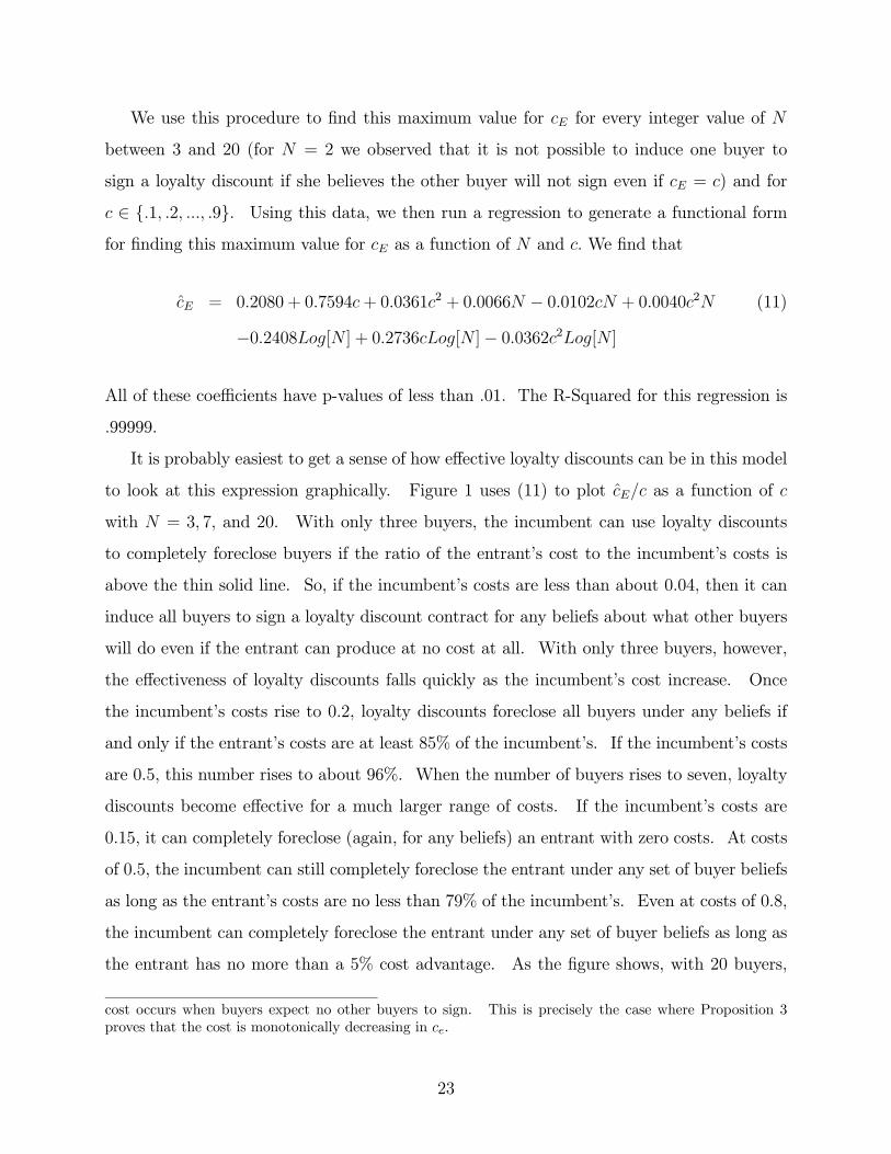
It is probably easiest to get a sense of how effective loyalty discounts can be in this model

to look at this expression graphically. Figure 1 uses (11) to plot as a function of

with = 3 7 and 20. With only three buyers, the incumbent can use loyalty discounts

to completely foreclose buyers if the ratio of the entrant’s cost to the incumbent’s costs is

above the thin solid line. So, if the incumbent’s costs are less than about 0.04, then it can

induce all buyers to sign a loyalty discount contract for any beliefs about what other buyers

will do even if the entrant can produce at no cost at all. With only three buyers, however,

the effectiveness of loyalty discounts falls quickly as the incumbent’s cost increase. Once

the incumbent’s costs rise to 0.2, loyalty discounts foreclose all buyers under any beliefs if

and only if the entrant’s costs are at least 85% of the incumbent’s. If the incumbent’s costs

are 0.5, this number rises to about 96%. When the number of buyers rises to seven, loyalty

discounts become effective for a much larger range of costs. If the incumbent’s costs are

0.15, it can completely foreclose (again, for any beliefs) an entrant with zero costs. At costs

of 0.5, the incumbent can still completely foreclose the entrant under any set of buyer beliefs

as long as the entrant’s costs are no less than 79% of the incumbent’s. Even at costs of 0.8,

the incumbent can completely foreclose the entrant under any set of buyer beliefs as long as

the entrant has no more than a 5% cost advantage. As the figure shows, with 20 buyers,

cost occurs when buyers expect no other buyers to sign. This is precisely the case where Proposition 3

proves that the cost is monotonically decreasing in

23

foreclosure under any beliefs is even easier, especially if the incumbent’s costs are not too

large.

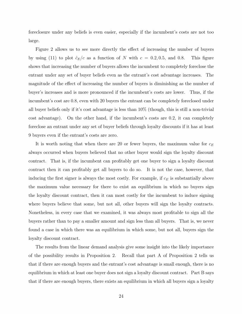
Figure 2 allows us to see more directly the effect of increasing the number of buyers

by using (11) to plot as a function of with = 02 05 and 08. This figure

shows that increasing the number of buyers allows the incumbent to completely foreclose the

entrant under any set of buyer beliefs even as the entrant’s cost advantage increases. The

magnitude of the effect of increasing the number of buyers is diminishing as the number of

buyer’s increases and is more pronounced if the incumbent’s costs are lower. Thus, if the

incumbent’s cost are 0.8, even with 20 buyers the entrant can be completely foreclosed under

all buyer beliefs only if it’s cost advantage is less than 10% (though, this is still a non-trivial

cost advantage). On the other hand, if the incumbent’s costs are 0.2, it can completely

foreclose an entrant under any set of buyer beliefs through loyalty discounts if it has at least

9 buyers even if the entrant’s costs are zero.

It is worth noting that when there are 20 or fewer buyers, the maximum value for

always occurred when buyers believed that no other buyer would sign the loyalty discount

contract. That is, if the incumbent can profitably get one buyer to sign a loyalty discount

contract then it can profitably get all buyers to do so. It is not the case, however, that

inducing the first signer is always the most costly. For example, if is substantially above

the maximum value necessary for there to exist an equilibrium in which no buyers sign

the loyalty discount contract, then it can most costly for the incumbent to induce signing

where buyers believe that some, but not all, other buyers will sign the loyalty contracts.

Nonetheless, in every case that we examined, it was always most profitable to sign all the

buyers rather than to pay a smaller amount and sign less than all buyers. That is, we never

found a case in which there was an equilibrium in which some, but not all, buyers sign the

loyalty discount contract.

The results from the linear demand analysis give some insight into the likely importance

of the possibility results in Proposition 2. Recall that part A of Proposition 2 tells us

that if there are enough buyers and the entrant’s cost advantage is small enough, there is no

equilibrium in which at least one buyer does not sign a loyalty discount contract. Part B says

that if there are enough buyers, there exists an equilibrium in which all buyers sign a loyalty

24

discount contract. Our linear demand results make four main points that demonstrate that

these possibility results likely have significant practical impact. These are summarized in

the following remark.

Remark With linear demand and 20 or fewer buyers:

1. If the incumbent can profitably induce one buyer to sign a loyalty discount contract then

it can profitably create a unique equilibrium in which all buyers sign a loyalty discount

contract.

2. If the entrant’s cost advantage is small, it takes only three buyers to create this unique

exclusionary equilibrium.

3. The larger the potential market (based on demand when price equals cost), the easier it

is for the incumbent to create this unique exclusionary equilibrium.

4. The incumbent can create a unique exclusionary equilibrium for a substantial range of

parameters even if the entrant has a non-trivial cost advantage. For example, if the

entrant has no more than a 10% cost advantage, the incumbent can create a unique

exclusionary equilibrium with three buyers if its costs are less than 28% of the choke

price, with seven buyers if its costs are less than 68% of the choke price, and with 20

buyers if its costs are less than 80% of the choke price.

In our model, with zero costs of entry, entry is always efficient. Thus, our linear demand

results show that there is substantial scope for an incumbent to profitably use loyalty dis-

counts to foreclose efficient entry, reducing both productive efficiency and consumer surplus.

Notice that this occurs, unlike in prior models of exclusive dealing, without any economies

of scale and even with buyers with independent demands.

2.4.2 Numerical Analysis—Optimal Loyalty Discount

In this part, instead of analyzing the conditions under which some loyalty discount contract

can exclude an entrant, we analyze what loyalty discount would be optimal for the incumbent

given that using loyalty discounts is profitable for the incumbent. As with determining the

25

conditions for exclusions, we proceed via numerical anlaysis. In this case, we randomly

drew parameter values for the incumbent’s cost, , the entrant’s cost, and the number

of buyers, . We drew from a uniform distribution between zero and one. We drew

from a uniform distribution between {0 2− 1} and This ensures both that the

entrant’s innovation is non-drastic and that it has a cost advantage over the incumbent.17

We drew from the integers between three and 20 with each one equally likely. For each

set of parameters that we drew, we calclulated, as above, the discount, that minimized the

incumbent’s maximum cost of signing each buyer, assuming that the each buyer assumed

that the number of other buyers who would sign the loyalty discount contract was the number

that would maximize the cost of inducing buyers to sign the contract.18 Thus, for each set

of paramter values, we determined the optimal discount and the cost of signing up buyers

under the assumption that each buyer’s belief about the number of other buyers who would

sign the contract is that which would maximize the signing cost.

We did 1500 draws from these distributions of parameter values. Of these 1500 draws,

using loyalty discounts was profitable (and effectively excluded the entrant) in just over half

of the draws (763).19 We used these 763 cases to analyze (using linear regression analysis)

the optimal loyalty discount in situations where the incumbent would use them. We found

that a relatively simple, and easy to interpret specification, explained over 90 percent of the

variation in the optimal discount (R-squared of 901):

= 0023− 0091− 0430 + 0201[ ] (12)

All coefficients are significant at the 05 level and the coefficients of and [ ] are

significant at well-beyond the 001 level. This tells us that the incumbent offers contracts

with higher discounts the more firms there are.20 Increasing both the entrant’s and the

17This restriction on the entrant’s cost is actually somewhat weaker than Assumption (∗), which explainswhy loyalty discounts were not profitable in so many cases.18We make this assumption to examine the worst case for loyalty discounts for the incumbent.19Not surprisingly, given the results in the last subsection, the cases where loyalty discounts were not

profitable were those where the entrant’s cost advantage was large and the number of buyers was small, and

the market was small.20Recall, that this result does depend on buyers making the worst-case assumption that the number

of other buyers who will agree to the loyalty commitment is the number that maximizes the cost of the

26

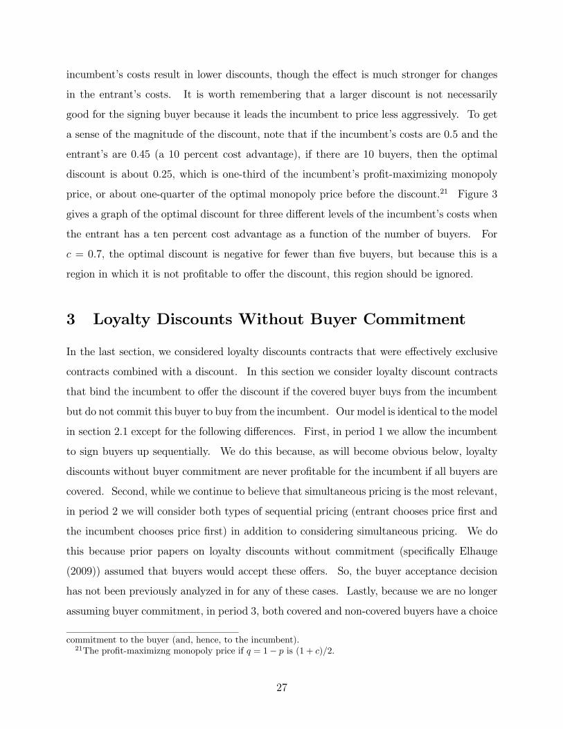
incumbent’s costs result in lower discounts, though the effect is much stronger for changes

in the entrant’s costs. It is worth remembering that a larger discount is not necessarily

good for the signing buyer because it leads the incumbent to price less aggressively. To get

a sense of the magnitude of the discount, note that if the incumbent’s costs are 05 and the

entrant’s are 045 (a 10 percent cost advantage), if there are 10 buyers, then the optimal

discount is about 025 which is one-third of the incumbent’s profit-maximizing monopoly

price, or about one-quarter of the optimal monopoly price before the discount.21 Figure 3

gives a graph of the optimal discount for three different levels of the incumbent’s costs when

the entrant has a ten percent cost advantage as a function of the number of buyers. For

= 07 the optimal discount is negative for fewer than five buyers, but because this is a

region in which it is not profitable to offer the discount, this region should be ignored.

3 Loyalty Discounts Without Buyer Commitment

In the last section, we considered loyalty discounts contracts that were effectively exclusive

contracts combined with a discount. In this section we consider loyalty discount contracts

that bind the incumbent to offer the discount if the covered buyer buys from the incumbent

but do not commit this buyer to buy from the incumbent. Our model is identical to the model

in section 2.1 except for the following differences. First, in period 1 we allow the incumbent

to sign buyers up sequentially. We do this because, as will become obvious below, loyalty

discounts without buyer commitment are never profitable for the incumbent if all buyers are

covered. Second, while we continue to believe that simultaneous pricing is the most relevant,

in period 2 we will consider both types of sequential pricing (entrant chooses price first and

the incumbent chooses price first) in addition to considering simultaneous pricing. We do

this because prior papers on loyalty discounts without commitment (specifically Elhauge

(2009)) assumed that buyers would accept these offers. So, the buyer acceptance decision

has not been previously analyzed in for any of these cases. Lastly, because we are no longer

assuming buyer commitment, in period 3, both covered and non-covered buyers have a choice

commitment to the buyer (and, hence, to the incumbent).21The profit-maximizng monopoly price if = 1− is (1 + )2

27

of supplier if entrant has entered. If − ≤ then only free buyers purchase from

and covered buyers purchase from . Thus, ’s profit is ( − − )( − ) while ’s

profit is (1− )( − )() If then all buyers purchase from Thus, ’s profit

is ( − − )( − ) + (1− )( − )() while ’s profit is zero. If − ≥ then

all buyers purchase from and thus ’s profit is ( − )() and ’s profit is zero. In

what follows, in the interest of reducing notation, we will ignore integer constraints on the

number of buyers covered.

3.1 Entrant Chooses Price First

If the entrant chooses a price then the incumbent will either choose = − and sell

to the entire market or it will choose = +− and sell only to covered buyers. Letting → 0 we have that the incumbent sells only to covered buyers if and only if the following

holds:

( − )()− {( − − )( − ) + (1− )( − )()} ≥ 0 (13)

Clearly, the entrant would never choose a price for which this condition does not hold,

because then it would earn zero profits. The left hand side is decreasing in as long as

profits are concave in prices and Furthermore, the left hand side is clearly positive

at = for any 0 Thus, the incumbent will sell only to covered buyers so long as the

entrant chooses a small enough price (which can exceed ). If the discount is large enough,

it is possible that the incumbent will sell only to covered buyers even if = Let be

the price that satisfies (13) at equality if it exists and is smaller than or alternatively,

By totally differentiating (13) with repsect to we can determine how varies with

for :

=

2( − )()− ( − − )( − )

(1− 2){() + ( − )0()}+ {( − ) + ( − − )0( − )} 0

This is positive for 12 because the incumbent’s profit is greater at than − because ≤ and because the incumbent’s profit is increasing at both and − . Thus, for

28

12 (and for larger we can see that = ), is increasing in That is, the higher

the share of buyers covered by the loyalty discount, the higher the price the entrant can

choose without the incumbent undercutting this price for non-covered buyers (which would

eliminate the entrant’s profit). Thus, (13) implicitly defines as a non-decreasing (strictly

increasing when ≤ ) function of

The entrant can also choose = and sell to all buyers. It will prefer to choose if

and only if:

(1− )( − )()− (− )() ≥ 0 (14)

Clearly, this is only satisfied if the fraction of covered buyers, is not too large.

The entrant will never choose a price higher than To see if loyalty discounts

without commitment can support this price, note that (14) implies a maximum theta of

=( −)( )−(−)()

( −)( ) Next, we see if we can satisfy (13) at If the entrant’s innova-

tion satisfies Assumption (∗) (so that ), then 0 If there is no restriction on

and 0 (13) can always be satisfied because the incumbent’s loss from selling to even one

covered buyer at a price of − can be made arbitrarily large by making arbitrarily large

(so that the incumbent has to pay the covered buyer an arbitrarily large amount to buy the

good).

Alternatively, one might imagine that − must be non-negative (the incumbent cannotoffer a negative price to covered buyers) or that − ≥ (the incumbent cannot price below

cost to covered buyers). If we impose the first constraint, then loyalty discounts can support

the entrant choosing if and only if:

(2 − 1)( − )( ) + (0) ≥ 0 (15)

The reason is that if this inequality is satisfied, then the incumbent earns more profit from

selling only to covered buyers at the entrant’s monopoly price than it would earn from selling

to uncovered buyers at the entrant’s monopoly price and selling to covered buyers at a price

of zero (which would give it losses of (0)). The left hand side of this is increasing in

This is clearly satisfied for any ≥ 12 and could be satisfied for much lower if theincumbent’s losses at a price of zero are substantial. If we impose the second constraint (no

29

predatory pricing), then loyalty discounts can support the entrant choosing if and only

if ≥ 12 Let = ( −)( )2( −)( )+(0) We have now proven the following lemma.

Lemma 3 If the discounted price must be non-negative, then loyalty discounts without buyer

commitment can support an entrant price of if ∈ [ ] If the discounted pricecannot be below , then loyalty discounts without buyer commitment can support an

entrant price of if ∈ [12 ] In either case, the incumbent just undercuts tocovered buyers and does not sell to uncovered buyers.

It remains to be seen whether or not the incumbent can induce this fraction of buyers to

agree to be covered by a loyalty discount. While one might think that this is trivial because

agreeing to the discount involves does not bind a buyer, this is does not mean that agreeing

is necessarily costless to the buyer. As the fraction of covered buyers increases, as long as

it is below or 12 the greater is the price the entrant will choose. Because the incumbent

chooses a price so that the discounted price just undercuts the entrant’s price, this means

that agreeing to be covered by the discount can increase the price the buyer expects to pay

if the buyer expects that enough other buyers will choose not to be covered by the discount.

In this case, the incumbent might have to pay buyers to induce them to be covered.

Whether this will be possible will depend on the number of buyers and the entrant’s cost

advantage. If there are only two buyers, for example, then buyers will never agree to be

covered by loyalty discounts without buyer commitment for any upfront payment that the

incumbent would be willing to make. The incumbent would never want to cover both buyers

because then the entrant would have to charge to stop the incubment from undercutting it.

If the incumbent signs up only one buyer, then this buyer loses consumer surplus because

of the higher price, but the incumbent only gains from the higher price through sales to

this one buyer. Because elevating prices above costs is inefficient (increased profits are less

than lost consumer surplus), the incumbent cannot pay one buyer to accept. With only

one covered buyer, there is no negative externality on other buyers that the incumbent can

benefit from (there is a negative externality, but this benefits the entrant who sells to the

non-covered buyer at a higher price). With more buyers, however, it is possible for the

incumbent to profitably induce enough buyers to sign the loyalty discount contract so that

30

prices are elevated to as long as the entrant’s cost advantage is not too great.

Proposition 4 (A) If there is no constraint on , then the incumbent can induce buy-

ers to be covered by a loyalty discount without buyer commitment in exchange for an

arbitrarily small payment if ≥{2 ()−( )( −)( )} leading to = and − =

− (B) If the discounted price is constrained to be non-negative, then the incumbentcan induce buyers to be covered by a loyalty discount without buyer commitment

in exchange for an arbitrarily small payment if ≥ {(()−( ))( −)( ) } This

condition will always be met if demand is concave and the entrant’s cost advantage is

sufficiently small. When this condition is met, prices will be = and − =

− (C) If the discounted price is constrained to not be below , then the incumbent

can induce buyers to be covered by a loyalty discount without buyer commitment

in exchange for an arbitrarily small payment if ≥ {2(()−( ))2( −)( ) } This

condition will always be met if demand is concave and the entrant’s cost advantage is

sufficiently small. When this condition is met, prices will be = and − =

−

Proof. (A) By choosing an arbitrarily large the incumbent can guarantee that (13) is

satisfied at for any 0 Thus, the incumbent will respond to the entrant’s price of by

offering = +− and selling only to covered buyers. The entrant will choose ratherthan (which would enable it to sell to all buyers) as long as ≤ Thus, the incumbent’s

can maximize its profit by getting buyers to be covered by the discount. It only remains

to show that these buyers will accept the discount for an arbitrarily small payment. To

show this, consider the case in which − buyers have rejected the incumbent’s offer.

If the next buyer believes that all future buyers will also reject, then she will accept the

discount if she is paid ()− ( ) her loss of consumer surplus from paying a price of

rather than . Because (13) can be satisfied at for large enough even after only one

buyer has signed, all subsequent buyers know that their decision to be covered will not affect

equilibrium prices. So, none of these buyers need more than a trivial payment to accept the

discount. Thus, even if − buyers have already rejected the incumbent’s discount, the

incumbent can get the remaining buyers covered with only a total payment of ()− ( )

31

This is profitable so long as ()− ( ) (( − )( )) This never holds if 2

Because the first − expect the incumbent to sign buyers even if they reject the

incumbent’s offer, rejecting the offer does not increase their consumer surplus. Hence, the

first buyer approached will accept being covered for only a trivial sidepayment, which means

that all subsequent buyers approached will also.

(B) First, we define the following terms to simplify the later notation. Let =

( − )( ) be the entrant’s monopoly profit per buyer. Let

= ( − )() be the

entrant’s profit per buyer if it charges a price of . Let = ( − )( ) be the

incumbent’s profit per buyer it serves at the entrant’s monopoly price. Let 0 = () be

the incumbent’s loss per buyer it serves at a price of zero.

If the incumbent cannot charge a negative price, then the maximum loss it can suffer

from selling to covered buyers is (0) Given this, the entrant will choose if and only if

the fraction of covered buyers is at least but less than Thus, once the incumbent has

covered buyers, all remaining buyers up until do not require compensation to be

covered because they will pay the same price, , whether they are covered or not because

the entrant will offer a price of once there are covered buyers but not more than

covered buyers. We will assume the worst case for making such compensation profitable.

Specifically, we will ask if the incumbent can obtain agreement to be covered from buyers

when − buyers have already rejected the offer. We will then assume that remaining

buyers believe that if they reject the incumbent’s offer, then all future buyers will reject, but

if they accept, then enough buyers will accept ( buyers) so that they will face a price

of . Lastly, contrary to fact, we will assume that even when some buyers have already

accepted, until buyers have accepted, the buyers believe that rejecting the offer will

enable them to buy at the competitive price of . We make this assumption simply because

for a general demand curve, we cannot get an explicit formula for as a function of the

number of buyers who have already accepted. Thus, buyers must receive compensation

of ()− ( )

This means it is profitable for the incumbent to get buyers to accept if:

− (()− ( )) 0 (16)

32

Substituting for and we can write this as:

−

−

2 + 0

(()− ( )) 0

We know that ()− ( ) =

Z

() ( − )() Thus, a sufficient condition is:

( − )(2 + 0)− (

− )() 0

It is easy to see that if the entrant’s innovation is almost drastic (so that is only

slightly larger than ) , − close to zero, then this sufficient condition will not hold.

On the other hand, if the entrant’s cost advantage is very small, almost zero and is

almost as big as , then this is [

0+( −)(2( )−())] This is always positive if is concave because the monopoly quantity exceeds half the competitive quantity for concave

demand.

As in (A), because the first − expect the incumbent to sign buyers even if they

reject the incumbent’s offer, rejecting the offer does not increase their consumer surplus.

Hence, the first buyer approached will accept being covered for only a trivial sidepayment,

which means that all subsequent buyers approached will also.

(C) This follows from the proof of (B) because this proof continues to be valid if we take

0 = 0 as would be the case if the discounted price equals the incumbent’s cost. Q.E.D.

If the incumbent can offer an arbitrarily large discount, then the incumbent never wants

to sell to both covered and non-covered buyers because charging a price that meets the

entrant’s price for non-covered buyers will result in arbitrarily large losses from selling to

each covered buyer. Thus, having one covered buyer is sufficient to ensure that prices are at

the entrant’s monopoly price. So, once the incumbent has signed up one buyer, all remaining

buyers expect to pay the entrant’s monopoly price whether they are covered or not. Hence

they will sign up for a trivial side-payment. In order to ensure that one buyer will sign up,

the incumbent has to be willing to pay that one buyer her loss of consumer surplus from

paying the monopoly price rather than the competitive price. But, if it is profitable to do

so, the incumbent needn’t actually pay this amount because buyers prior to − expect

33

the incumbent to offer buyer − her lost consumer surplus to sign (() − ( )), so

they might as well sign for any amount.

If the incumbent’s discount is constrained so that it cannot offer a negative price, then

its loss per covered buyer is bounded, hence it needs to sign up more buyers to ensure it does

not have an incentive to undercut the entrant’s price of To eliminate an equilibrium

in which all buyers reject being covered thinking that all subsequent buyers will reject, the

incumbent has to be able to reimburse buyers for their loss in consumer surplus out of

the profits of selling to covered buyers at the entrant’s monopoly price. The buyers’ loss

in consumer surplus is less than ()−( ) each.22 Thus, if − (()−( )) 0

the incumbent always has a credible threat to sign up a sufficient number of buyers.

One might think that this is easier to satisfy as the entrant’s costs are smaller because

the lost consumer surplus is smaller. However, smaller entrant costs also reduce the

maximum fraction of buyers that can be covered without the entrant charging and selling

to all buyers. It turns out that this latter effect matters more when the entrant’s innovation

is close to drastic ((16) is decreasing in when is such that = ). But, if the

entrant’s costs are close to the incumbent’s23 and demand is concave, then the incumbent

can always induce enough buyers to agree to be covered for a trivial side-payment, leading

the market to be divided between the incumbent and the entrant, with all buyers paying the

entrant’s optimal monopoly price. Thus, even without commiting buyers to buy only from

the incumbent, if the entrant prices first, loyalty discounts can lead to a divided market and

higher prices.

3.2 Incumbent Chooses Price First

If the incumbent chooses its price to free buyers, , first, then the entrant will either choose

to price at = { } —selling only to uncovered buyers—or the entrant will choose

22If the first buyer to sign believes that her signing will induce all the others to sign, but that none will

sign if she does not, then her lost consumer surplus from signing is exactly () − ( ) All subsequent

buyers have a smaller lost consumer surplus since even if all later buyers reject, the price will be elevated

above due to the earlier buyers being covered. Thus, ()− ( ) is an upper bound on the lost consumer

surplus per buyer.23(16) is increasing in at = so satisfying this condition becomes harder as falls from .

34

={− } and sell to all buyers. Because the incumbent makes zero profit in thelatter case, for any given fraction of covered buyers, , the incumbent must choose a price

such that the entrant prefers to sell only to uncovered buyers. That is, must satisfy:

(1− )( − )()− ( − − )( − ) ≥ 0 (17)

Unlike when the entrant chooses price first, here the left hand side of (17) is decreasing

in which means that the that satisfies (17) at equality is decreasing in Furthermore,

notice that if (17) holds, covered buyers pay − while uncovered buyers pay{ }Thus, unlike when the entrant prices first, here agreeing to be covered is a dominant strategy

for buyers as long as one buyer will be covered. Whether or not the incumbent must pay

to cover one buyer if all other buyers have rejected being covered depends on the pricing

equilibrium with no covered buyers. With no covered buyers, the incumbent earns zero for

any price ≥ and loses money on any lower price. Thus, there is no unique equilibrium

with no covered buyers: buyers could face any price between and because the incum-

bent has zero sales and profits for any price in this region.24 It will be the most difficult for

the incumbent to get buyers to agree to be covered by a loyalty discount if they believe the

equilibrium with no covered buyers will result in a price of In that case, the incumbent

would have to be willing to pay one buyer compensation. But, if buyers believe the incum-

bent will do that, then all buyers will agree to be covered for no compensation because they

expect at least one covered buyer and they pay lower prices if they sign up both because

covered buyers pay less than uncovered ones and because both prices are lower when there

are more covered buyers.

Thus, the incumbent can certainly cover any fraction of buyers at no cost so long as it

could profitably compensate one buyer for its lost consumer surplus (and possibly without

needing to be able to profitably compensate any buyers). Ignoring the cost of compensating

one buyer, the incumbent’s profit from covering a fraction, of buyers is (−−)(−)where and must be such that (17) holds. If we assume there are no constraints on then

24We do not necessarily get the Bertrand equilibrium since (unlike with simultaneous pricing), the entrant

will adjust its price based on the incumbent’s to ensure the incumbent has zero sales for any price above .

35

we can restrict attention to = and − = 25 (17) then implies that the highest

discounted price the incumbent can charge is given by (−)() = (1−)( −)( )With these substitutions, we totally differentiate (17) with respect to to obtain:

= − ( − )(

)

()− ( − )0()

We then use this in differentiating the incumbent’s profit to obtain the first order condition

for :

=( − )(){()− ( − )

0()}( − )( ){()− ( − )0()} (18)

The right hand side of (18) is increasing in At = we get = (− )()( −

)( ) = 1− , where the last equality follows from (17). This means that at = the

incumbent maximizes period 2 profits by covering half the buyers with loyalty discounts.

If the entrant has a cost advantage, then the incumbent will cover a smaller fraction of

the market with loyalty discounts. If the incumbent does have to be able to profitably

compensate one buyer, it can do so at = if () − () ≤ (2)( − )() where

is given by ( − )() = ( − )( )2.26 One might think that the incumbent

would choose a larger because while that would reduce period 3 profits, it would reduce

the amount of compensation required to ensure one buyer agrees to be covered. That isn’t

the case, however, because the incumbent does not have to actually pay this compensation.

As long as it would be willing to compensate enough buyers, buyers will agree to be covered

for no compensation because they expect the number of other buyers that will be covered

will be such that uncovered buyers will pay Whereas, if they agree to be covered, they

will pay We have now proved the following result.

Proposition 5 If the incumbent chooses price first, it will cover a fraction of buyers ≤ 12by a loyalty discount without buyer commitment and covered buyers will agree to be

25The incumbent would never want to choose a discount that did not enable to entrant to capture all

uncovered buyers at its monopoly price since that would simply force the incubment to choose a lower

discounted price in order to ensure the entrant did not wish to compete for all buyers.26This is the largest discounted price (if = ) the incumbent can charge for which the entrant weakly

prefers to sell to half the buyers at its monopoly price than to sell to all the buyers at the incumbent’s

discounted price.

36

covered for no compensation if () − () ≤ ( − )() where is given by

( − )() = (1 − )( − )( ) The fraction of buyers that will be covered

is increasing in and is 12 at = Covered buyers will pay which is strictly

greater than but strictly less than Uncovered buyers will pay

Thus, if the incumbent chooses price first, then it can use loyalty discounts without buyer

commitment to ensure that it makes positive profits and continues to serve a fraction of the

market despite its higher costs. Whether consumer’s pay higher prices or not depends on

what the equilibrium outcome is absent loyalty discounts, which is uncertain given that there

is a continuum of equilibria.

3.3 Simultaneous Pricing

We now consider the case of in which the entrant and incumbent choose their prices simul-

taneously in period 2. It turns out that this case has a great deal in common with the case

in which the incumbent chooses price first.

As was the true in the commitment case, the pricing equilibrium here must be in mixed

strategies. To see this, imagine that the entrant chose a price . Then the incumbent

would choose a discounted price (−) just below in order to sell to covered buyers. The

entrant’s best response to such a price, however, would be either to match it or choose

and sell only to uncovered buyers. Because the entrant’s best response to a price just below

would be to match it, there can be no pure strategy equilibrium.

We first assume that the discount, , is large enough that the incumbent cannot profitably

compete for buyers who did not accept the loyalty discount (uncovered buyers), even if the

entrant prices at its monopoly level. We establish that this is optimal for the incumbent

in the appendix. To determine the mixed strategy equilibrium, notice that if the entrant’s

price distribution is given by the cumulative distribution function then the incumbent’s

expected period 2 profit from a discounted price of is (1−())(−)() We knowthat the entrant will never charge a price that exceeds nor will it ever charge a price

lower than 0 where 0 solves (0− )(0) = (1− )( − )( ) because the entrant can

37

always earn (1− )( − )( ) from selling only to uncovered buyers.27 Thus, must

be such that the incumbent can earn the same profit from charging = 0 and selling to

covered buyers with probability one or charging some other and selling to covered buyers

with probability 1− () That is:

(1− ())( − )() = (0 − )(0)

This implies that

() = 1− (0 − )(0)

( − )()(19)

with an atom at of(0−)(0)( −)( )

If the incumbent’s pricing distribution is given by the cumulative distribution function ,

then the entrant’s expected profit from charging a price of is (1− ())(− )() +

(1−)(−)() The entrant sells to all uncovered buyers as long as the discount is largeenough that the incumbent’s undiscounted price exceeds which the Appendix proves is

always the case. The entrant sells to covered buyers with probability 1− () The entrantcan always choose a price of and obtain profits of (1− )( − )(

) by only selling

to uncovered buyers.28 That is:

(1− ())( − )() + (1− )( − )() = (1− )( − )( )

This implies that

() =( − )()− (1− )( − )(

)

( − )()(20)

Notice that the 0 the minimum of both price distributions, is decreasing in (the

condition for 0 implies that 0 = −( − )( ){(0) + (0 − )

0(0)}); () is

decreasing in 0 (and the atom at is increasing in 0); and () is increasing in This

27Since 0 ≥ this creates a maximum for the mixed strategy equilibrium. For any above this

maximum, the entrant will charge with probability one. Obviously, any above this maximum will not

be in the interest of the incumbent, since it will earn zero profits. The maximum = 1− (−)()( −)( )

28In equilibrium,the incumbent’s maximum price cannot exceed the entrant’s maximum price or the in-

cumbent would make no profits. Thus, the entrant only sells to uncovered buyers at its maximum price.

Given this, the entrant’s maximum price must be

38

means that the larger the fraction of covered buyers, the lower the prices (in expectation)

that buyers will face from both the entrant and the incumbent. Thus, once one buyer

is covered, other buyers strictly prefer to be covered than uncovered. Hence, as was the

case when the incumbent chose price first, the incumbent need only be able to profitably

compensate one buyer in order to induce as many buyers as it wants to be covered. In

this case, however, the unique equilibrium with no covered buyers is the competitive one, so

there is no doubt about the fact that the incumbent must be able to profitably compensate

one buyer.

Once again, then, we simply need to determine the fraction of covered buyers that max-

imizes the incumbent’s profits given the pricing distributions. The incumbent’s expected

profit is simply (0 − )(0) (because he can charge 0 and sell to all covered buyers with

probability one). Using the expression for 0 in the last paragraph, the first order

condition for is:

=(0 − )(0){(0) + (0 − )

0(0)}( − )( ){(0) + (0 − )0(0)}

Notice, this is the exact same condition for as when the incumbent chose price first (see

equation (18)) with replaced by 0 But, also notice the condition for 0 here is identical

for the condition for in the last subsection. Hence, the optimal fraction of buyers that

the incumbent will choose to cover is identical (it will be exactly half if = and less than

half if the entrant has a cost advantage). The only difference between the equilibria in the

two cases is that (i) the incumbent’s price is higher in the simultaneous pricing case because

instead of charging = 0 with probability one, he charges price drawn from a distribution

between 0 and ; and (ii) the entrant’s price is lower because instead of charging with

probability one, it charges a price drawn from a distribution between 0 and Thus,

uncovered buyers are better off under simultaneous pricing but covered buyers are worse off

relative to the case in which the incumbent chooses price first.

Given that the incumbent’s period 2 profits are identical in the two cases as is the fraction

of covered buyers, we have proven the following result.

Proposition 6 If the incumbent and entrant choose price simultaneously, the incumbent

will cover a fraction of buyers ≤ 12 by a loyalty discount without buyer commitment

39

and covered buyers will agree to be covered for no compensation if () − (0) ≤(0 − )(0) where 0 is given by (0 − )(0) = (1 − )( − )(

) The

fraction of buyers that will be covered is increasing in and is 12 at = Both

covered and uncovered buyers will pay a price between 0 and

This proposition establishes that with simultaneous pricing, the incumbent can use loy-

alty discounts without buyer commitment to prevent the entrant from capturing the entire

market, leading both to production inefficiency and prices that are elevated above the com-

petitive level along with the associated allocation inefficiency. In fact, as we have seen,

we get similar results no matter what the period 2 pricing game is. While, without buyer

commitment, loyalty discounts cannot exclude the entrant from the entire market, they can

ensure that the incumbent retains positive market share (despite its relative inefficiency) and

maintain supra-competitive prices.

The above proposition assumes that the incumbent has chosen a large enough discount

that, in equilibrium, even if the entrant charges its monopoly price, it will sell to all uncovered

buyers. We show in the appendix that the incumbent will not choose a smaller discount that

does not satisfy that property. We do this by showing that, with any discount that does not

satisfy that property, there exists an equilibrium in which the incumbent earns lower profits.

4 Conclusion

This article has shown that loyalty discounts (which involve seller commitments to charge

loyal buyers less than disloyal buyers) can increase prices and/or block entry. Strikingly,

this result is possible under any demand curve, even if the entrant is more efficient than

the incumbent,and without any entry costs or economies of scale, and even if the buyers

are final consumers (or otherwise have independent demand). It can also occur with or

without buyer commitment. With buyer commitment, unless the entrant cost advantage is

sufficiently large, this equilibrium will always occur for a sufficient number of buyers. With

linear demand, and an entrant cost advantage of less than 10%, an incumbent can profitably

foreclose the entire market with as few as three buyers unless incumbent costs are more than

28% of the choke price. Not only are prices raised but a more efficient rival is kept off the

40

market. Without buyer commitment, the rival will not be kept off the market entirely, but

supracompetitive pricing will result as long as the entrant’s cost advantage is not too great.

These results show that the intuition that loyalty discounts presumptively reduce prices

is misplaced. Loyalty “discounts” are just the difference between loyal and disloyal pricing,

and thus need not signify any true discount from the but-for prices that would have existed

but for the loyalty discounts. In fact, this model shows that loyalty discounts encourage

incumbents to raise prices above but for levels and discourage discounting to free buyers.

These results also disprove the intuition that above-cost loyalty discounts cannot exclude an

equally efficient rival. Here, above-cost loyalty discounts can exclude the rival even though

the rival is in fact more efficient than the incumbent. Further, it can do so even though there

are no economies of scale that might mean the rival has been relegated to a high cost portion

of its cost curve. These results also disprove the claim that voluntary buyer agreement means

the agreement must enhance the welfare of buyers. In fact, we show that loyalty discounts

(either with or without commitment) can have anti-competitive effects even if buyers can

coordinate on their preferred equilibrium.

Our results have important implications for competition policy. Antitrust enforcers

should scrutinize loyalty discounts with buyer commitment in situations in which ordinary

exclusive dealing might not be of concern (independent buyers, no economies of scale).

Antitrust enforcers should not view loyalty discounts more favorably if buyer coordination is

likely; it does not eliminate the potential for anti-competitive effects from loyalty discounts.

Loyalty discounts without buyer commitment can also have anti-competitive effects, even

though they are not likely to be completely exclusionary and may sometimes even increase

the entrant’s profits. In addition, antitrust enforcers should not take the fact that only a

minority of buyers are covered by loyalty discounts as evidence that it is not having an anti-

competitive effect. Loyalty discounts with buyer commitment can have anticompetitive

effects even when they cover a minority of the market, and for loyalty discounts without

commitment, covering a minority of buyers is part the incumbent’s optimal anticompetitive

strategy.

Our model assumes that the incumbent only offers a discount off a price to be determined

later. We explained above, in footnote 10, why specifying price in advance might not be

41

possible (this is the standard assumption in the exclusive dealing literature). That said, if

the incumbent could offer a contract that specified price in advance, this would not be as

profitable for the incumbent unless the contract somehow linked the price it offered to loyal

buyers to the price if offered to disloyal buyers. It is this linking of price that creates the

externality across buyers that allows the incumbent to retain market share and earn profits

even though this reduces total welfare. If the incumbent could credibly commit to a price to

both loyal buyers and disloyal buyers, then it could effectively deter entry and capture most

of the consumer surplus. It would do this by commiting to charge disloyal buyers a price

above the entrant’s monopoly price and charging loyal buyers its marginal cost in exchange

for a payment of ()−( ) However, such a commitment, even if in a contract, might notbe credible, if buyers are independent, because breaching the seller commitment to charge

disloyal buyers a high price would not create any damages for anyone.

A few limitations should, however, be stressed. First, we have assumed a market with

only one potential rival. This can often be the case, especially in high-tech or pharmaceutical

markets, but if there were multiple rivals with similar costs it is possible they would compete

prices down to their costs. However, the same sort of analysis seems likely to apply to the

extent only one entrant has a potential cost advantage and the other rivals have higher costs

and merely provide a competitive fringe. Multiple rivals might also use loyalty discounts

themselves, creating similar or even exacerbated market segmentation effects.29 But it re-

mains for future work to extend the model here to cases involving multiple rivals or where

multiple firms use loyalty discounts.30

Second, when analyzing loyalty discounts with buyer commitments, we have assumed

that buyers always honor their commitments. The analysis would get more complicated if

we considered the possibility that buyers could freely breach their commitments. However,

as we have discussed above, if buyers must pay damages for breach of contract when they

breach their loyalty commitments, then this would often deter breach, and even if it does

not, it does not eliminate the ability of the incumbent to profitably use loyalty discount

contracts to reduce competition.31 Moreover, as Elhauge (2009) has pointed out, there may

29See Elhauge (2009) at pp. 195, 214-15 for a discussion of these issues.30See Kitamura (2010) for an argument that naked exclusion is less effective if there are multiple entrants.31Note that Elhauge (2009) finds that, under linear demand, loyalty commitments will induce rivals to

42

be many reasons why the legal or extralegal penalties for breach exceed expectation damages.

Further, we find that loyalty discounts can have anticompetitive effects without any buyer

commitments.

Lastly, we have assumed loyalty discounts have no efficiencies. If they did, those might

offset any adverse effects. It seems likely the present model can be extended to show how

much of a cost reduction would be necessary to offset the anticompetitive effects, but that

also remains a matter for future work.

5 Appendix

Proof of Proposition 1. (i) Inspection of (4) makes it clear that it does not depend on

Because increasing increases however, the atom in the entrant’s distribution at

is now spread out between [ 0 ] 0 is also not affected by (see (5)). Differen-

tiating (8) with respect to gives(−0)(0)(−)2() 0 Thus, for any the probability

that the incumbent charges a price less than is increasing in for There is a

new atom at 0 and positive probability up to 0 (ii) Differentiating (6) with respect to

gives− (−)()+(−)+()[()+(−)0()](1−)(−)2() 0 This is negative because the term in

square brackets in the numerator is zero because maximizes profits and and 0

only affects the incumbent’s pricing distribution, (9), through its effect on 0 Because

0 increasing 0 decreases () for any Totally differentiating (5) with respect

to and solving for 0gives 0

=

(1−)(0)+((0−)−())+()[()+(−)0()](1−)[(0)+(0−)0(0)]+[(0−)+(0−−)0(0−)] 0

This is positive because 0 , 0 and () + ( − )0() = 0. So, increas-

ing increases 0 which reduces () for any . (iii) only affects the incum-

bent’s pricing through its effect on 0 Totally differentiating (5) with respect to and

solving for 0gives 0

=

(0−)(0)+(−)()−(0−−)(0−)(1−)[(0)+(0−)0(0)]+[(0−)+(0−−)0(0−)]

0 So, increas-

ing increases 0 which reduces () for any . Differentiating (6) with respect

to gives − (−)()−(−−)(−)(1−)(−)2() 0 So, increasing reduces the probability that

the entrant chooses a price below any given level . (iv) only affects the in-

cumbent’s pricing through 0 Totally differentiating (5) with respect to and solving

price sufficiently above cost that expectation damages will deter breach.

43

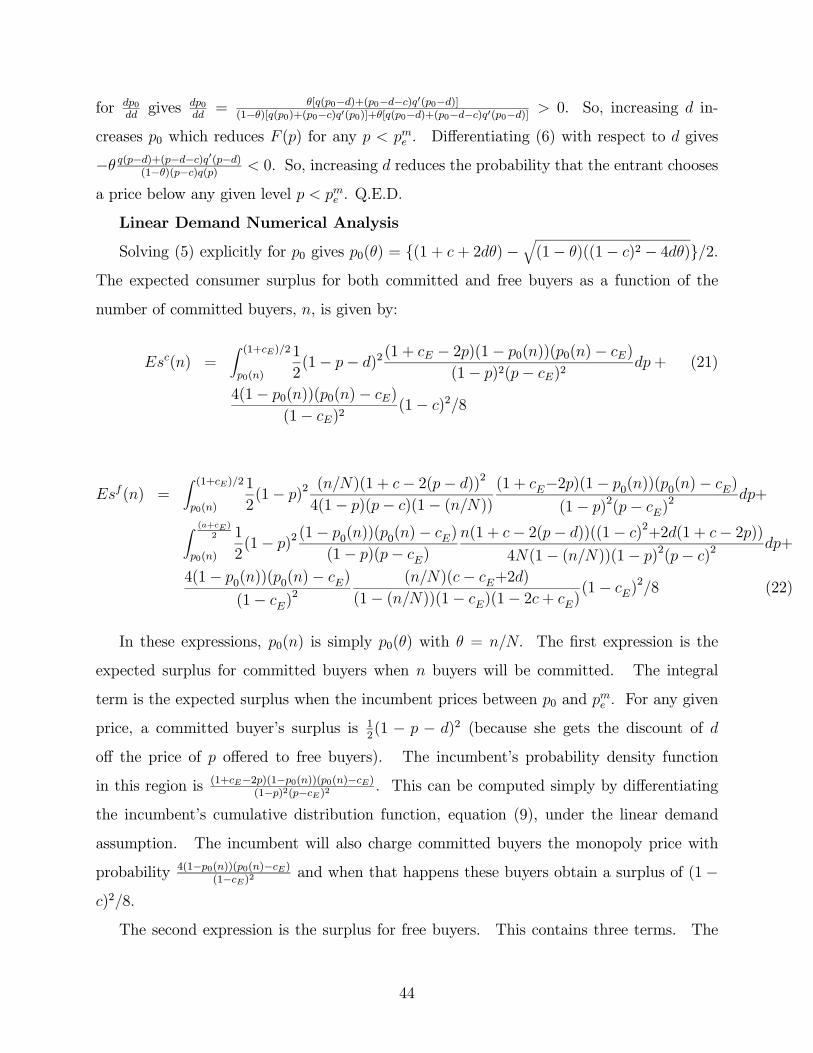
for 0gives 0

=

[(0−)+(0−−)0(0−)](1−)[(0)+(0−)0(0)]+[(0−)+(0−−)0(0−)] 0 So, increasing in-

creases 0 which reduces () for any . Differentiating (6) with respect to gives

− (−)+(−−)0(−)(1−)(−)() 0 So, increasing reduces the probability that the entrant chooses

a price below any given level . Q.E.D.

Linear Demand Numerical Analysis

Solving (5) explicitly for 0 gives 0() = {(1 + + 2)−q(1− )((1− )2 − 4)}2

The expected consumer surplus for both committed and free buyers as a function of the

number of committed buyers, , is given by:

() =

Z (1+)2

0()

1

2(1− − )2

(1 + − 2)(1− 0())(0()− )

(1− )2(− )2+ (21)

4(1− 0())(0()− )

(1− )2(1− )28

() =

Z (1+)2

0()

1

2(1− )

2 ()(1 + − 2(− ))2

4(1− )(− )(1− ())(1 + −2)(1− 0())(0()− )

(1− )2(− )

2 +

Z (+)

2

0()

1

2(1− )

2 (1− 0())(0()− )

(1− )(− )

(1 + − 2(− ))((1− )2+2(1 + − 2))

4(1− ())(1− )2(− )

2 +

4(1− 0())(0()− )

(1− )2

()(− +2)

(1− ())(1− )(1− 2+ )(1− )

28 (22)

In these expressions, 0() is simply 0() with = The first expression is the

expected surplus for committed buyers when buyers will be committed. The integral

term is the expected surplus when the incumbent prices between 0 and For any given

price, a committed buyer’s surplus is 12(1 − − )2 (because she gets the discount of

off the price of offered to free buyers). The incumbent’s probability density function

in this region is(1+−2)(1−0())(0()−)

(1−)2(−)2 This can be computed simply by differentiating

the incumbent’s cumulative distribution function, equation (9), under the linear demand

assumption. The incumbent will also charge committed buyers the monopoly price with

probability4(1−0())(0()−)

(1−)2 and when that happens these buyers obtain a surplus of (1−)28

The second expression is the surplus for free buyers. This contains three terms. The

44

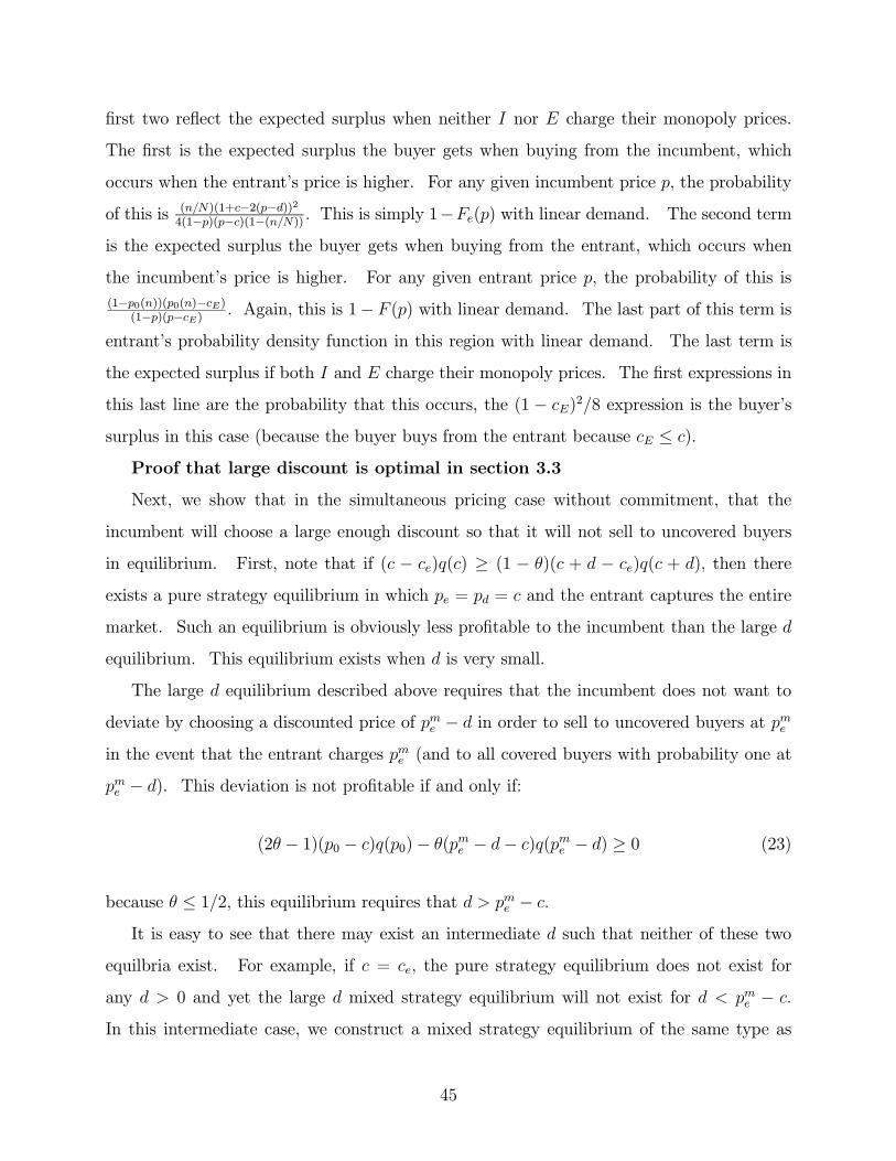
first two reflect the expected surplus when neither nor charge their monopoly prices.

The first is the expected surplus the buyer gets when buying from the incumbent, which

occurs when the entrant’s price is higher. For any given incumbent price the probability

of this is()(1+−2(−))24(1−)(−)(1−()) This is simply 1−() with linear demand. The second term

is the expected surplus the buyer gets when buying from the entrant, which occurs when

the incumbent’s price is higher. For any given entrant price the probability of this is

(1−0())(0()−)(1−)(−) Again, this is 1− () with linear demand. The last part of this term is

entrant’s probability density function in this region with linear demand. The last term is

the expected surplus if both and charge their monopoly prices. The first expressions in

this last line are the probability that this occurs, the (1 − )28 expression is the buyer’s

surplus in this case (because the buyer buys from the entrant because ≤ ).

Proof that large discount is optimal in section 3.3

Next, we show that in the simultaneous pricing case without commitment, that the

incumbent will choose a large enough discount so that it will not sell to uncovered buyers

in equilibrium. First, note that if ( − )() ≥ (1 − )( + − )( + ) then there

exists a pure strategy equilibrium in which = = and the entrant captures the entire

market. Such an equilibrium is obviously less profitable to the incumbent than the large

equilibrium. This equilibrium exists when is very small.

The large equilibrium described above requires that the incumbent does not want to

deviate by choosing a discounted price of − in order to sell to uncovered buyers at

in the event that the entrant charges (and to all covered buyers with probability one at

− ). This deviation is not profitable if and only if:

(2 − 1)(0 − )(0)− ( − − )( − ) ≥ 0 (23)

because ≤ 12 this equilibrium requires that −

It is easy to see that there may exist an intermediate such that neither of these two

equilbria exist. For example, if = the pure strategy equilibrium does not exist for

any 0 and yet the large mixed strategy equilibrium will not exist for −

In this intermediate case, we construct a mixed strategy equilibrium of the same type as

45

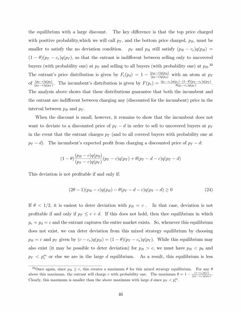
the equilibrium with a large discount. The key difference is that the top price charged

with positive probability,which we will call and the bottom price charged, , must be

smaller to satisfy the no deviation condition. and still satisfy ( − )() =

(1 − )( − )( ) so that the entrant is indifferent between selling only to uncovered

buyers (with probability one) at and selling to all buyers (with probability one) at 32

The entrant’s price distribution is given by () = 1 − (−)()(−)() with an atom at

of (0−)(0)(−)( ) The incumbent’s distribution is given by () =

(−)()−(1−)(−)( )(−)()

The analysis above shows that these distributions guarantee that both the incumbent and

the entrant are indifferent between charging any (discounted for the incumbent) price in the

interval between and

When the discount is small, however, it remains to show that the incumbent does not

want to deviate to a discounted price of − in order to sell to uncovered buyers at

in the event that the entrant charges (and to all covered buyers with probability one at

− ). The incumbent’s expected profit from charging a discounted price of − :

(1− )( − )()

( − )( )( − )( ) + ( − − )( − )

This deviation is not profitable if and only if:

(2 − 1)( − )()− ( − − )( − ) ≥ 0 (24)

If 12 it is easiest to deter deviation with = . In that case, deviation is not

profitable if and only if ≤ + If this does not hold, then thee equilibrium in which

= = and the entrant captures the entire market exists. So, whenever this equilibrium

does not exist, we can deter deviation from this mixed strategy equilibrium by choosing

= and given by (− )() = (1− )( − )( ) While this equilibrium may

also exist (it may be possible to deter deviation) for we must have 0 and

or else we are in the large equilibrium. As a result, this equilibrium is less

32Once again, since ≥ this creates a maximum for this mixed strategy equilibrium. For any

above this maximum, the entrant will charge with probability one. The maximum = 1− (−)()(−)( )

Clearly, this maximum is smaller than the above maximum with large since

46

profitable for the incumbent than the large equilibrium.

It is worth pointing out that the equilibrium in this case is different from the equilib-

rium described in Elhauge (2009) for simultaneous pricing without commitment and a small

discount. In Elhauge’s proposed equilibrium, the incumbent could profitably deviate by

charging a discounted price just below the support of his distribution that allows him to

sell to uncovered buyers with non-zero probability because the entrant has an atom in its

distribution at its highest price.

References

[1] Aghion, Philippe, and Patrick Bolton. 1987. “Contracts as a Barrier to Entry.” American

Economic Review, 77(3): 388—401.

[2] Argention, Cedric. 2010. ”Exclusive Quality.” Journal of Industrial Economics, 58:690-

716.

[3] Bernheim, B. Douglas, and Michael D. Whinston. 1998. “Exclusive Dealing.” Journal

of Political Economy, 106(1): 64—103.

[4] Butz, David A. 1990. “Durable-Good Monopoly and Best-Price Provisions,” American

Economic Review 80: 1062-76.

[5] Chen, Zhijun and Greg Shaffer. 2010. ”Naked Exclusion with Minimum Share Re-

quirements,” Working Paper.

[6] Cooper, Thomas E. 1986. “Most-Favored-Customer Pricing and Tacit Collusion,” The

RAND Journal of Economics 17: 377-388.

[7] Edlin, Aaron. 1997. ”Do Guaranteed-Low-Price Policies Guarantee High Prices, and

Can Antitrust Rise to the Challenge?”, Harvard Law Review 111: 528-575.

[8] Elhauge, Einer. 2003. “Defining Better Monopolization Standards.” Stanford Law Re-

view 56: 253-344.

47

[9] Elhauge, Einer. 2008. United States Antitrust Law & Economics. Foundation Press:

New York.

[10] Elhauge, Einer. 2009. “How Loyalty Discounts Can Perversely Discourage Discounting,”

Journal of Competition Law & Economics 5: 189-231.

[11] Farrell, Joseph. 2005. “Deconstructing Chicago on Exclusive Dealing,” Antitrust Bul-

letin 50: 465-480 (2005).

[12] Fumagalli, Chiara, and Massimo Motta. 2006. “Exclusive Dealing and Entry, when

Buyers Compete.” American Economic Review, 96(3):785—95.

[13] Hovenkamp, Herbert. 2005. Antitrust Law Vol.. XI (2d ed.).

[14] Hovenkamp, Herbert. 2006. “Discounts and Exclusion.” Utah Law Review, 2006: 841-

861.

[15] Hviid, Morten and Greg Shaffer. 2010. ”Matching Own Prices, Rivals’ Prices or Both?”

Journal of Industrial Economics, 58:479—506.

[16] Innes, Robert, and Richard J. Sexton. 1994. “Strategic Buyers and Exclusionary Con-

tracts.” American Economic Review, 84(3): 566—84.

[17] Kaplow, Louis & Carl Shapiro. 2007. “Antitrust,” in Handbook of Law & Economics 2:

1073-1225 (eds. Polinsky & Shavell).

[18] Kitamura, Hiroshi. 2010. ”Exclusionary Vertical Contracts with Multiple Entrants.”

International Journal of Industrial Organization, 28:213-219.

[19] Kolay, Sreya, Greg Shaffer, and Janusz A. Ordover. 2004. ”All-Units Discounts in

Retail Contracts,” Journal of Economics and Management Strategy, 13:429-459.

[20] Lambert, Thomas A.. 2005. “Evaluating Bundled Discounts.” Minnesota Law Review,

89: 1688-1757.

[21] Lin, Y. Joseph. 1990. ”The Dampening of Competition Effect of Exclusive Dealing,”

Journal of Industrial Economics, 39:209-223.

48

[22] Mahenc, Philippe and Francois Salanie. 2004. ”Softening Competition Through For-

ward Trading,” Journal of Economic Theory, 116:282-293.

[23] Marx, Leslie M. & Greg Shaffer. 2004. “Opportunism in Multilateral Vertical Contract-

ing: Nondiscrimination, Exclusivity, and Uniformity: Comment,” American Economic

Review 94: 796-801.

[24] Marx, Leslie M. & Greg Shaffer. 2004. “Rent-Shifting, Exclusion, and Market-Share

Discounts,” Working Paper.

[25] Mathewson, G. Frank, and Ralph A. Winter. 1987. “The Competitive Effects of Vertical

Agreements: Comment.” American Economic Review, 77(5): 1057—62.

[26] Neeman, Zvika. 1999. “The Freedom to Contract and the Free-Rider Problem.” Journal

of Law, Economics, and Organization, 15(3): 685—703.

[27] Ordover, Janusz and Greg Shaffer. 2007. ”Exclusionary Discounts,” Working Paper.

[28] Rasmusen, Eric B., J. Mark Ramseyer, J., and John S, Wiley. 1991. ”Naked Exclusion”,

American Economic Review, 81(5):1137—45.

[29] Rey, Patrick and Joseph E. Stiglitz. 1995. ”The Role of Exclusive Territories in Pro-

ducers’ Competition,” The RAND Journal of Economics 26: 431-451.

[30] Schnitzer, Monika. 1994. “Dynamic duopoly with best-price clauses,” The RAND Jour-

nal of Economics 25: 186-196.

[31] Segal, Ilya R., and Michael Whinston. 2000. “Naked Exclusion: Comment.” American

Economic Review, 90: 296-309.

[32] Simpson, John and Abraham L. Wickelgren. 2007. “Naked Exclusion, Efficient Breach,

and Downstream Competition.” American Economic Review, 97: 1305-1320.

[33] Spector, David. 2005. “Loyalty Rebates: An Assessment of Competition Concerns and

a Proposed Structured Rule of Reason,” Competition Policy International 1(2): 89-114

(Autumn).

49

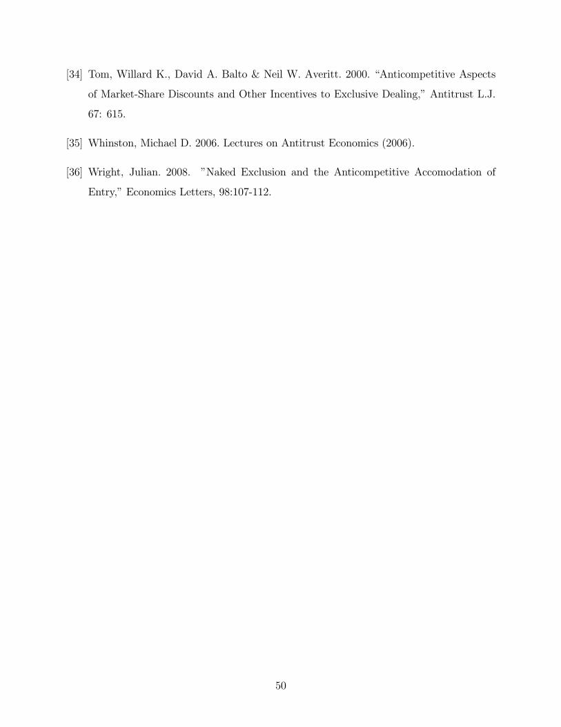
[34] Tom, Willard K., David A. Balto & Neil W. Averitt. 2000. “Anticompetitive Aspects

of Market-Share Discounts and Other Incentives to Exclusive Dealing,” Antitrust L.J.

67: 615.

[35] Whinston, Michael D. 2006. Lectures on Antitrust Economics (2006).

[36] Wright, Julian. 2008. ”Naked Exclusion and the Anticompetitive Accomodation of

Entry,” Economics Letters, 98:107-112.

50

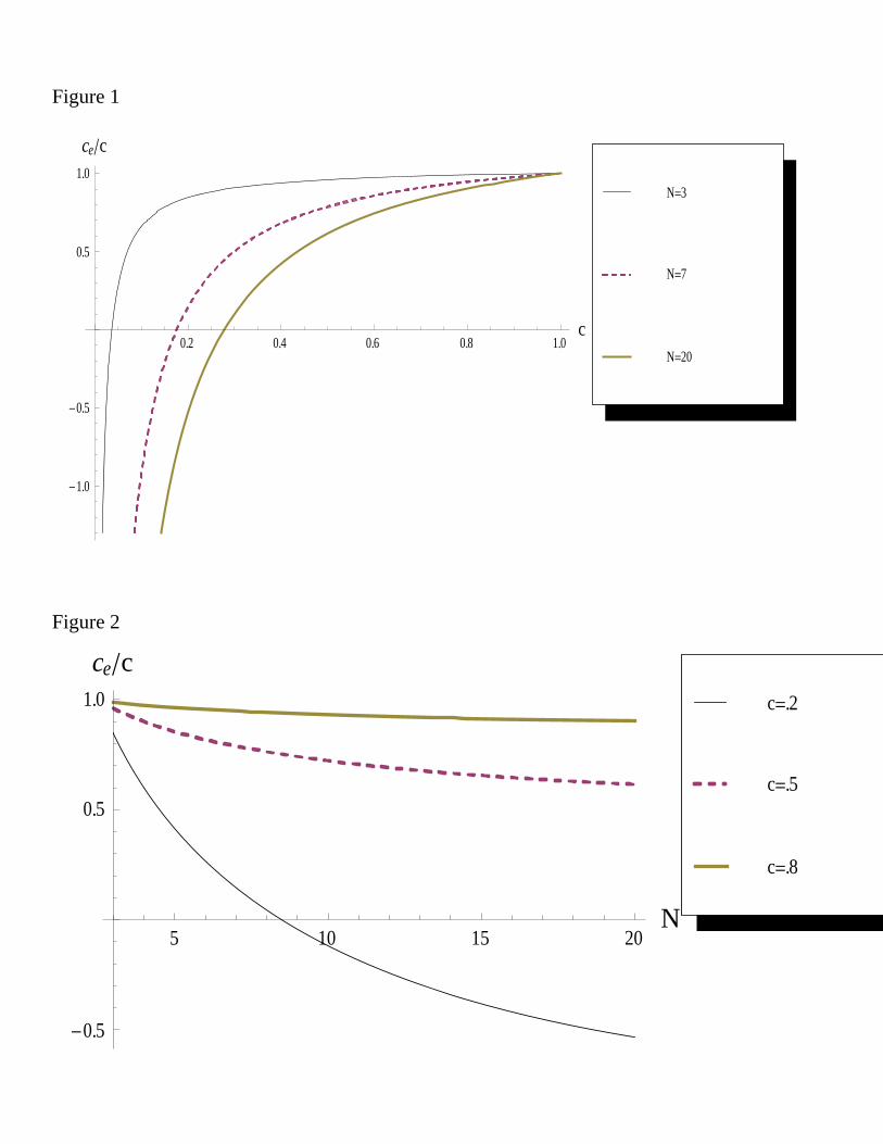
Figure 1

Figure 2

0.2 0.4 0.6 0.8 1.0c

-1.0

-0.5

0.5

1.0

cec

N=20

N=7

N=3

5 10 15 20N

-0.5

0.5

1.0

cec

c=.8

c=.5

c=.2

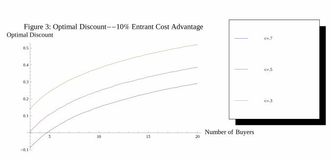
5 10 15 20Number of Buyers

-0.1

0.1

0.2

0.3

0.4

0.5

Optimal DiscountFigure 3: Optimal Discount--10% Entrant Cost Advantage

c=.3

c=.5

c=.7