Anthropogenic Reduction of Santa Ana winds

Mimi Hughes, Alex Hall, and Jinwon Kim∗

UCLA, Los Angeles, California

∗Corresponding author address: Mimi Hughes, University of California, Los Angeles, Box , Los Angeles, CA

90095.

E-mail: mhughes@atmos.ucla.edu

Abstract

The frequency of Santa Ana wind events is investigated within a high-resolution

downscaling of the ERA40 Reanalysis to 6-km resolution overSouthern California.

In this climate reconstruction, the number of Santa Ana daysper winter season de-

clines significantly over the 44-year reanalysis period, resulting in over 30% fewer

events per year over the final decade of the reconstruction (1991–2001) compared

to the first decade (1959–1969). We investigate this signal further in late-20th and

mid-21st century realizations of the NCAR CCSM3 global climate change sce-

nario run downscaled to 12-km resolution over California. The reduction in events

per year in the mid-21st century compared with the late-20thcentury is similar

to that seen in the ERA40 downscaling, suggesting the cause of the decrease is a

change in the climate due to anthropogenic forcing. A regression model is used to

reproduce the Santa Ana time series based on two previously-documented forcing

mechanisms: synoptically-forced strong offshore winds atthe mountain tops which

transport offshore momentum to the surface, and a local desert-ocean temperature

gradient causing katabatic-like winds as the cold desert air pours down the coastal

topography. Both past and future climate simulations show alarge reduction in the

contribution of the local thermodynamic forcing. This reduction is due to the differ-

ential warming that occurs during transient climate changeconditions, with more

warming in the desert interior than over the ocean. Thus the mechanism responsi-

ble for the decrease in Santa Ana frequency originates from awell-known aspect of

the climate response to increasing greenhouse gases, but cannot be understood or

simulated without mesoscale atmospheric dynamics.

1

1. Introduction

The cool, moist fall and winter climate of Southern California is often disrupted by dry,

hot, days with strong winds, known as Santa Anas, blowing outof the desert. The Santa Ana

winds are a dominant feature of the fall and wintertime climate of Southern California (Conil

and Hall 2006), and have important ecological impacts. First, and most pronounced, is their

influence on wildfires: following the hot, dry Southern California summer, the extremely low

relative humidities and gusty strong winds that occur during Santa Anas introduce extreme

fire risk which often culminates in wildfires with large economic loss (Westerling et al. 2004).

Less familiar but just as important is their impact on coastal-ocean ecosystems: The strong

winds induce cold filaments in sea-surface temperature (SST) with an associated increase in

biological activity (Castro et al. 2006; Trasvina et al. 2003). This decrease in SST and increase

in biological activity is likely due in part to increased mixing in the oceanic boundary layer,

although an increase in dust deposition on the ocean surfaceduring these events could also

increase biological activity (Hu and Liu 2003; Jickells et al. 2005).

Despite their importance to local climate, very few studiesexamine their variability on

timescales longer than a few months (Finley and Raphael 2007; Raphael 2003; Schroeder et al.

1964; Edinger et al. 1964). Furthermore, all but the oldest of these studies rely on a large-scale

proxy for the local Santa Ana wind intensity, which may not berepresentative of actual changes

to their frequency (Hughes and Hall 2008). In a recent study,Miller and Schlegel (2006) docu-

mented how Santa Ana wind frequency may change under anthropogenic climate change condi-

tions; however, similar to the above-mentioned studies, they use a large-scale proxy to indicate

their occurrence.

This study investigates the response of the frequency and intensity of Santa Ana events to an-

2

thropogenic climate change. Unlike previous studies, we identify Santa Ana wind events by the

strength of the offshore wind through the gaps in Southern California’s topography. To accom-

plish this local perspective, we downscale the ECMWF reanalysis data and a coarse-resolution

climate model with regional atmospheric models. This dynamical downscaling technique has

been proven numerous times to give a more realistic view of local climate conditions (e.g.,

Diffenbaugh et al. 2005; Leung and Ghan 1999), and when utilized with reanalysis products,

provide a reasonably accurate representation of a region’sclimate (Conil and Hall 2006; Hughes

et al. 2008; Hughes and Hall 2008; Kanamitsu and Kanamaru 2007a,b). Our results indicate

that as the climate begins to adjust to increased greenhousegas forcing, the frequency of Santa

Ana days is reduced.

A recent investigation of the dynamics of Santa Ana winds (Hughes and Hall 2008) found

that both local and synoptic conditions control their formation. Similar to the results of Gabersek

and Durran (2006), when strong synoptically forced offshore flow impinges on Southern Cali-

fornia’s topography, offshore momentum can be transportedto the surface, causing Santa Ana

conditions. However, Hughes and Hall (2008) found that there are many days with Santa Ana

conditions that are not associated with this type of strong synoptic forcing. Rather, for a large

fraction of the Santa Ana days, offshore winds are forced by alocal temperature gradient be-

tween the cold desert and warmer air over the ocean at the samealtitude. The temperature

gradient induces a hydrostatic pressure gradient pointingfrom the desert to the ocean, which

is reinforced by the negative buoyancy of the cold air as it flows down the sloped surface of

the major topographical gaps. This mechanism is essentially the same the one driving katabatic

winds of Antarctica (Parish and Cassano 2003; Barry 1992). Often both mechanisms are at

play, because the synoptic conditions causing strong offshore flow aloft – a high pressure sys-

3

tem over the northwestern US coast – also favor cold advection into the desert. This is most

often the case during the strongest Santa Ana days. As we demonstrate, this understanding of

the dynamics of Santa Ana winds allows us to identify how large-scale changes in the future

climate affect the frequency and intensity of Santa Ana events.

2. Data

a. MM5 Simulation

Identification of events in the actual climate and weather conditions of the last half-century

is given by a high resolution simulation created with the Penn State/NCAR mesoscale model

version 5, release 3.6.0 (MM5 Grell et al. 1994). The 6 km domain was nested within an 18

km domain covering Southern California and parts of Arizona, Nevada, and Mexico, which

was likewise nested within a 54 km domain encompassing most of the western US. At this

resolution, all major mountain complexes in Southern California are represented, as are the

Channel islands just off the coast. The number of gridpointsin each domain are 35x36, 37x52,

and 55x97 for the 54, 18, and 6 km domains, respectively, and the nesting was two-way for both

interior domains. Each domain has 23 vertical levels, with the vertical grid stretched to place the

highest resolution in the lower troposphere. In the outer two domains, the Kain-Fritsch 2 (Kain

2002) cumulus parameterization scheme was used. In the 6km domain only explicitly resolved

convection could occur. In all domains, we used the MRF boundary layer scheme (Hong and

Pan 1996), Dudhia simple ice microphysics (Dudhia 1989), and a radiation scheme simulating

longwave and shortwave interactions with clear-air and cloud (Dudhia 1989).

The atmospheric boundary conditions for the simulation come from ECMWF’s 45-year

4

reanalysis data (ERA-40, Uppala et al. 2005) available through the National Center for At-

mospheric Research’s Computational and Information Systems Laboratory. The sea-surface

temperature (SST) comes from the Smith and Reynolds Extended Reconstructed SST dataset

for 1959-1980 (Smith and Reynolds 2003) and the NOAA OptimumInterpolation Sea Surface

Temperature Analysis after 1981 (Reynolds et al. 2002); theSST data was linearly interpolated

in time to 6-hour intervals. The time period covered in the simulation was from January 1959 to

August 2002. Throughout this period, MM5 was initialized every 15 days at 18Z (10 am local

time) and run for 366 hours, with the first six hours being discarded as model spin-up. The inte-

rior boundary conditions were updated at each initialization, with the sea-surface temperatures

and lateral boundary conditions updated continuously throughout the run. Thus the simulation

in the 6-km nest acts as a reconstruction of the local atmospheric conditions based on known

large scale atmospheric conditions.

The effectiveness of this downscaling technique in reconstructing local circulation anoma-

lies has been shown by two previous studies for a simulation with the same configuration but

different observational products as boundary conditions and shorter temporal extent. Corre-

lating the simulation’s daily-mean winds with available point measurements, Conil and Hall

(2006) verified that this shorter simulation captures synoptic time-scale variability in the daily-

mean wind. In addition, Hughes and Hall (2008) showed that the offshore component of the

wind (i.e., the component most aligned with the Santa Anas) was highly correlated with surface

observations throughout the domain.

5

b. WRF simulation

The dynamical downscaling for the climate change scenario was performed using the Weather

Research and Forecast (WRF) model, version 2.2.1 (Skamarock et al. 2005). Similar to MM5,

the model solves a non-hydrostatic momentum equation in conjunction with the thermody-

namic energy equation. The model features multiple optionsfor advection and the parameter-

ized atmospheric physical processes. The physics options selected in this experiment include

the NOAH land-surface scheme (Chang et al. 1999), the simplified Arakawa Schubert (SAS)

convection scheme (Hong and Pan 1998), the RRTM longwave radiation scheme (Mlawer et al.

1997), Dudhia (1989) shortwave radiation, and the WSM 3-class with simple ice cloud micro-

physics scheme. For more details on the physics options, readers are referred to the web site

http://wrf-model.org. The model domain covers the westernUnited States at a 36-km horizon-

tal resolution, with the inner 12-km nest spanning the entire coast of California. Both domains

have 28 atmospheric and 4 soil layers in the vertical.

The regional climate simulations were driven by the global climate data generated by the

NCAR CCSM3 when the SRES-A1B emission scenario is imposed (Nakicenovic and Swart

2000). The emission scenario assumes balanced energy generation between fossil and non-

fossil fuel; the resulting CO2 emissions are located near the averages of all SRES emission

scenarios. The climatology for the late 20th century and mid-21st century periods is calculated

from the 10 cold season (October-March) regional simulations for 1971-1981 and 2045-2055,

respectively. Individual runs were initialized at 00UTC October 1 of the corresponding years

using the CCSM-3 output data. All simulations continued forthe remaining 6 month period

without re-initialization by updating the large-scale forcing along the lateral boundaries at 3-

hour intervals.

6

Although the two downscalings are achieved using two different regional models – WRF and

MM5 – their dynamical cores and available physics packages are similar. The CO2 concentra-

tions in the WRF simulations were fixed at 330ppmv and 430ppmvduring the present-day and

mid-21st century periods, respectively, whereas the greenhouse gas concentrations in the MM5

downscaling are fixed for the 44-year simulation. However, increasing greenhouse gases in a

regional model has almost no effect on the climate unless thelarger-scale boundary conditions

also change. Thus the differences between the two WRF simulations are due to the different

boundary conditions (i.e., the large-scale response to increases greenhouse gases) and not to the

greenhouse gas increase in WRF itself. Further, the MM5 downscaling contains information

about the changing climate because of its reanalysis boundary conditions.

3. A Santa Ana Index

The first step in identifying the local and synoptic scale atmospheric conditions associated

with Santa Ana (SA) winds is to create a SA index. In the past, this has been done in numerous

ways. Two recent studies have used large scale surface pressure conditions, a high over the

Great Basin and a low southwest of Los Angeles, to identify Santa Ana events (Miller and

Schlegel 2006; Raphael 2003). Operational definitions combine this pressure gradient with two

other parameters, the relative humidity in coastal Southern California, and wind direction in

major mountain passes (Sommers 1978, D. Danielson 2007, personal communication). Conil

and Hall (2006) used a mixture model cluster analysis of the daily mean wind anomalies to

classify the winter circulation into three regimes, one of which was Santa Ana events.

For this study, we seek a SA index that does not introduce assumptions about large scale

7

mechanisms possibly causing Santa Anas. The operational and large-scale definitions do not

meet this criterion. Further, we also seek an index that gives information about SA intensity.

However, the cluster model classification technique gives no indication about the strength of the

offshore flow and rather simply classifies a day as experiencing Santa Ana conditions or not.

Since no previous metric meets our needs, we develop a new SA index based on the magnitude

of a spatially extensive offshore wind in the local circulation.

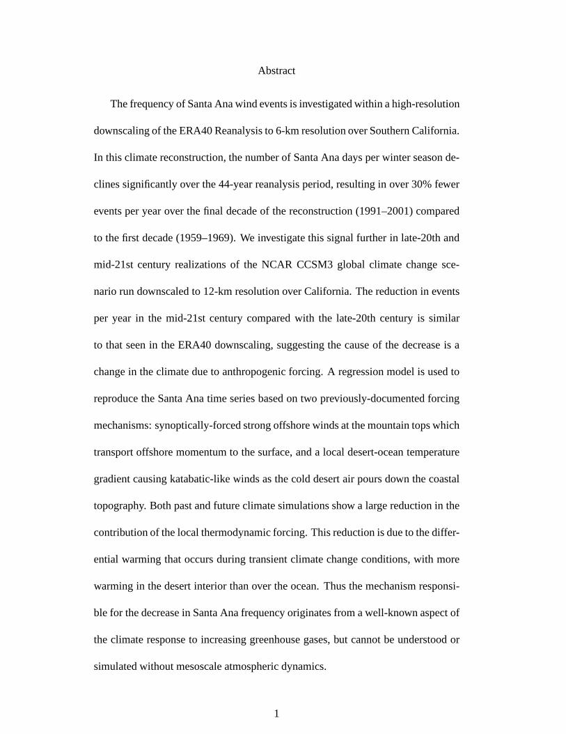
We create a SA index that is simply the offshore wind strengthat the exit of the largest gap

(blue box, Fig. 1a and b); the resulting time index, SAt, is shown for the MM5 simulation in

Fig. 1c. To illustrate that this index agrees with previous measures of SA intensity, Fig. 1a and

b show the composite surface winds for days with SAt greater than 8 m s-1for subsets of the

MM5 and WRF simulations, respectively. The composite SA wind fields exhibit characteristics

we expect for SA events: strong offshore (that is, roughly northeasterly) winds throughout most

of Southern California, with the strongest winds on the leeward slopes of the mountains and

through the gaps in the topography, most notably across the Santa Monica mountains.

Our index has a very strong seasonality (Fig. 1c), with peak occurrence in December and

no strong offshore winds from April to September. This agrees with previous indices of SA

occurrence (Hughes and Hall 2008; Conil and Hall 2006; Raphael 2003). Because of this strong

seasonality, from here on we only consider days between October and March and refer to them

as ’winter’ days.

8

4. Santa Ana response to a changing climate

Is there any change in the number of SA days due to anthropogenic forcing? To answer this

question, we first examine the frequency of SA wind events in the 44-year MM5 simulation.

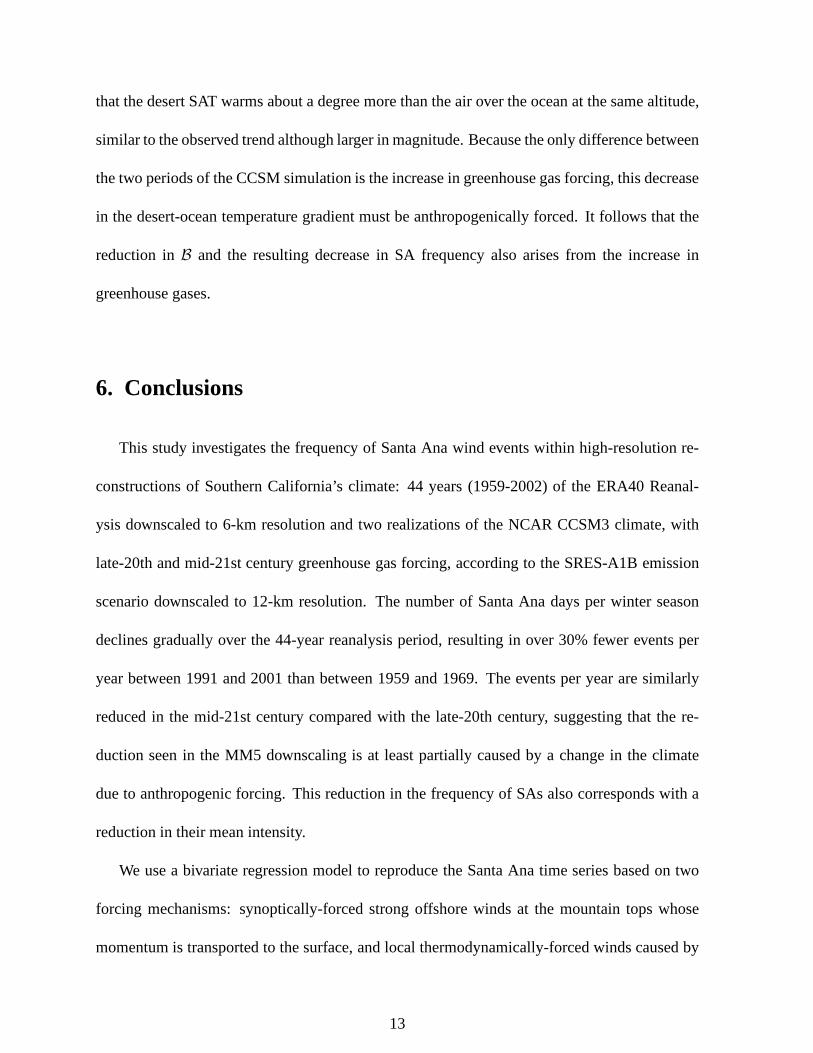
Fig. 2 shows the total number of winter days that have SAt greater than 6, 8, and 10 m s-1(blue,

red, and green lines). We show the results for 6 and 10 m s-1to illustrate that the results are not

sensitive to the threshold chosen as representing a SA day. There is a substantial decrease in the

number of SA days per winter season as we move from the 1960s tothe current century, with

the 1990s experiencing nearly 1/3 as many SA days as the 1960s.

This dramatic reduction in SA events over the last half of the20th century suggests that

increasing greenhouse gases and the associated climatic response could cause a change in SA

frequency. To test whether this change is indeed anthropogenic in origin, we now turn our

attention to SA days in the WRF downscaling of CCSM. To the extent that there is a difference

between the two WRF simulations, we know it is due to the effect of increased greenhouse

gases in the CCSM boundary conditions, since that is the onlydifference between the two

simulations. The inset panel of Fig. 2 shows the average number of days with SAt greater than

10 m s-1for the late-20th and mid-21st century WRF simulations; we use a larger threshold to

define a SA day in the WRF simulations because the WRF simulation has a slight climatological

bias towards stronger offshore winds, but the results are relatively insensitive to this threshold.

There is nearly a 20% reduction in the total number of SA days per year in the mid-21st century

run.

Because the CCSM-forced WRF simulation shows a qualitatively similar reduction in SA

wind occurrence to the MM5 run, the reduction in the MM5 downscaling is probably also due

to changes in the climate from anthropogenic forcing. In thefollowing sections, we explore the

9

mechanism by which the frequency of SA wind events is reducedto lend more credibility to

this result.

5. Understanding reduced Santa Ana frequency

The dynamics controlling the formation of SA winds were recently investigated by Hughes

and Hall (2008). They found that SAs arise from a combinationof two mechanisms: If there is

a large synoptic-scale pressure gradient causing strong offshore winds over Southern California

at mountain-top level, this causes strong surface flow as theoffshore momentum is transferred

to the surface. This often occurs when a high surface pressure anomaly is located over the

Great Basin. Alternatively, a large temperature gradient between the cold desert surface and the

warm ocean air at the same altitude (approximately 1.2 km) causes a localized offshore pressure

gradient near the surface. This in turn generates katabatic-like offshore flow in a thin layer near

the surface. These two mechanisms can act independently, causing mild SA winds, or combine

to force the largest magnitude offshore winds.

Hughes and Hall (2008) further developed a bivariate regression model to predict SAt based

on two parameters representative of each mechanism:

SAt(u,B) = A ∗ u + B ∗ B + C (1)

whereu, the offshore wind speed at 2-km, represents the synoptic forcing andB = gθ′

θ0

sin(α),

the katabatic pressure gradient (Parish and Cassano 2003),represents the local thermodynamic

forcing. In the equation forB, g = 9.8 m s-1 is gravitational acceleration,θ′ is the temperature

deficit of the cold layer,θ0 is the average temperature in the cold layer, andα is the slope

of the topography. To calculateB, we use the average desert surface temperature forθ0, the

10

average slope of the topography through the largest gap forα (approximately 1 degree, or 1 km

drop over 50 km; see Fig. 1a), and the temperature differencebetween the cold desert surface

(i.e., the cold layer) and air over the ocean at the same altitude (representative of the ambient

atmosphere) forθ′.

Fig. 3 shows the regression model’s representation of SAt,SAt, plotted against SAt for

the first and last decade of the MM5 downscaling (Fig.3a and b)and the WRF downscaling

simulations (Fig.3c and d). The high degree of correspondence (correlation coefficient = 0.91,

0.91, 0.88 and 0.86 for the two MM5 time periods and WRF present and future simulations,

respectively) confirms that the two mechanisms are primarily responsible for determining SAt in

all simulations. The coefficients of the model are similar within the two MM5 time periods and

the two WRF simulations (Table 1), but do vary somewhat with regional model. In particular,

the WRF simulations display larger sensitivity to variations in B (e.g., B=983 s-1for MM5

1959-1969 and B=2443 s-1for WRF present); this may partially explain the tendency for larger

SAt in those simulations.

Because it represents distinct physical processes, the regression model allows us to identify

the changes in forcing responsible for the reduction in SAt in both the observed time series

and the WRF climate change simulations. To understand whichterm of the regression model

is causing reducedSAt, we calculate the total contribution ofB andu to SAt separately and

then sum over days withSAt greater than 8 m s-1(14 m s-1) for the MM5 (WRF) time periods

(Fig. 4).

Turning our attention first to the synoptic forcing represented byu in Eq. 1 and the second

column grouping in Fig. 4, we see that the MM5 simulation shows a large reduction in contribu-

tion of synoptic forcing from the 1960’s to the 1990’s while the WRF simulation shows almost

11

no change between the present and future simulations. Because the synoptic activity often asso-

ciated with SA events often involves a high pressure system centered over the Great Basin at the

surface (e.g., Hughes and Hall 2008; Conil and Hall 2006; Raphael 2003), we examine the sea-

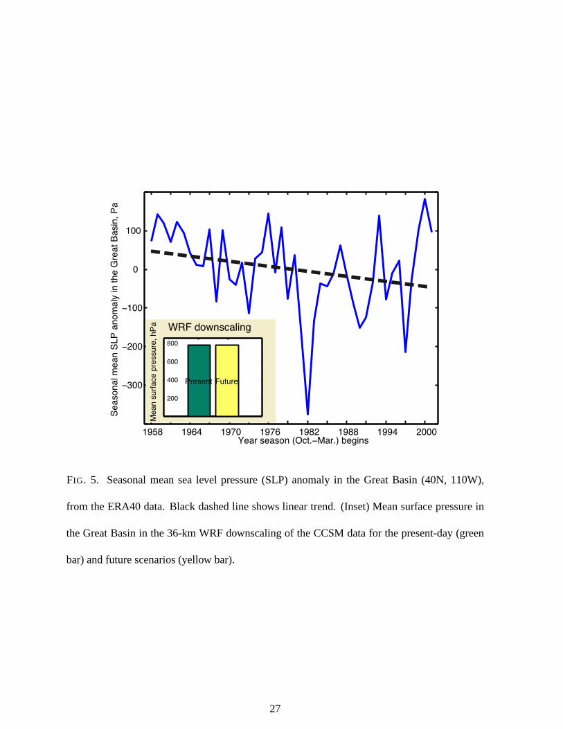
sonal mean sea-level pressure (SLP) anomaly in the Great Basin with the assumption that this is

representative of the synoptic variability on shorter timescales. The Great Basin SLP anomaly

in ERA40 shows a statistically significant negative trend over the last half century (Fig. 5), con-

sistent with the reduced synoptic forcing of SA winds seen inthe MM5 downscaling. However,

this reduction is absent in the WRF downscaling suggesting that this reduced synoptic forcing

is either not anthropogenically forced or is caused by a response to increased greenhouse gases

not captured by the CCSM simulations.

Focusing instead on the katabatic forcing ofB in Equ. 1 and the first column grouping

in Fig. 4, we see that both simulations show over 1/3 less contribution to SAt from B as the

climate responds to increased greenhouse gas forcing. Thisis because land masses respond

more quickly to increased radiative forcing than the oceans(e.g. Trenberth et al. 2007). Figure 6

shows the seasonal mean desert surface air temperature (SAT) as well as the air temperature

over the ocean at the same altitude – the two components ofθ′ used to calculateB – from the

MM5 simulation (main panel). Both temperatures show a positive trend over the 44-year time

series, but the desert surface air temperature increases more than the ocean temperature (note

that the trend of the air over the ocean is not significantly different from zero). The magnitude

of the katabatic pressure gradient,B, is directly proportional to the difference between these

two temperatures. So as the desert warms faster than the air over the ocean, a large temperature

gradient between the two areas becomes less likely in wintertime, and largeB becomes less

frequent. Examining the corresponding change in the WRF simulation (Fig. 6, inset), we see

12

that the desert SAT warms about a degree more than the air overthe ocean at the same altitude,

similar to the observed trend although larger in magnitude.Because the only difference between

the two periods of the CCSM simulation is the increase in greenhouse gas forcing, this decrease

in the desert-ocean temperature gradient must be anthropogenically forced. It follows that the

reduction inB and the resulting decrease in SA frequency also arises from the increase in

greenhouse gases.

6. Conclusions

This study investigates the frequency of Santa Ana wind events within high-resolution re-

constructions of Southern California’s climate: 44 years (1959-2002) of the ERA40 Reanal-

ysis downscaled to 6-km resolution and two realizations of the NCAR CCSM3 climate, with

late-20th and mid-21st century greenhouse gas forcing, according to the SRES-A1B emission

scenario downscaled to 12-km resolution. The number of Santa Ana days per winter season

declines gradually over the 44-year reanalysis period, resulting in over 30% fewer events per

year between 1991 and 2001 than between 1959 and 1969. The events per year are similarly

reduced in the mid-21st century compared with the late-20thcentury, suggesting that the re-

duction seen in the MM5 downscaling is at least partially caused by a change in the climate

due to anthropogenic forcing. This reduction in the frequency of SAs also corresponds with a

reduction in their mean intensity.

We use a bivariate regression model to reproduce the Santa Ana time series based on two

forcing mechanisms: synoptically-forced strong offshorewinds at the mountain tops whose

momentum is transported to the surface, and local thermodynamically-forced winds caused by

13

a katabatic pressure gradient that arises from the thermal contrast between cold desert surface

air and warmer air over the adjacent ocean. The regression model reproduces approximately

80% of the variability in the Santa Ana time index, and also reproduces the dramatic reduction

in events in the climate change experiment. We investigate the cause for the reduction of Santa

Ana frequency using the regression model to partition the forcing into synoptic and katabatic

components, and find a reduction in katabatic forcing in bothsimulations. This reduction of

katabatic forcing is caused by the larger transient response to increased radiative forcing of

desert surface air temperature than the air temperature over the ocean at the same altitude. This

reduces the likelihood of a large temperature deficit developing in the desert in wintertime and

therefore reduces the likelihood of large katabatic forcing.

There are many societal implications of this anthropogenicreduction of Santa Ana wind

events that could be significant and should be explored further. The role Santa Ana winds

play in spreading wildfire in the region (e.g., Westerling etal. 2004; Keeley 2004) suggests

their reduction in frequency could lead to reduced wildfire in Southern California. However,

they still occur in the future climate. Moreover, this studydoes not investigate other critical

fire parameters, such as available fuel and relative humidity depression during Santa Anas.

Meanwhile, ignition events (i.e., humans lighting matchesin the coastal chaparral shrubland),

another major factor affecting fire frequency, will probably increase with population (Syphard

et al. 2007). This study also has implications for coastal marine ecosystems, which respond

favorably to SA conditions, and to the air quality in the Los Angeles basin, which is better

during SA events. The ecological effects of nutrient loss for the Southern California Bight and

the decline in air quality during winter could be quantified with regional simulations of oceanic

biogeochemistry and atmospheric chemistry.

14

To the extent that the smaller temperature increase in the atmosphere over the ocean is

due to the larger oceanic heat capacity, the reduction in thermodynamic forcing of Santa Anas

might be a feature of the transient climate change that will return to pre-industrial levels once the

climate equilibrates. Nevertheless, the reduction in Santa Ana wind events due to anthropogenic

climate change is significant because it illustrates an observed and explainable regional change

in climate due to plausible mesoscale processes.

Acknowledgments.

Mimi Hughes is supported by the UCLA Dissertation Year Fellowship and NSF ATM-

0735056, which also supports Alex Hall. Part of this work wasperformed using NCAR su-

percomputer allocation 35681070. The research described in this paper was performed as an

activity of the Joint Institute for Regional Earth System Science and Engineering, through an

agreement between the University of California, Los Angeles, and the Jet Propulsion Labora-

tory, California Institute of Technology, and was sponsored by the National Aeronautics and

Space Administration. Preprocessing of the Community Climate System Model data was also

partially funded by the “National Comprehensive Measures against Climate Change” Program

by Ministry of Environment, Korea (Grant No. 1700-1737-322-210-13) National Institute of

Environmental Research, Korea. Computational resources for this study have been provided by

Jet Propulsion Laboratorys Supercomputing and Visualization Facility and the National Aero-

nautics and Space Administration (NASA) Advanced Supercomputing (NAS) Division.

15

References

Barry, R. G., 1992:Mountain Weather and Climate. Routledge, 402 pp.

Castro, R., A. Mascarenhas, A. Martinez-Diaz-de Leon, R. Durazo, and E. Gil-Silva, 2006:

Spatial influence and oceanic thermal response to Santa Ana events along the Baja California

peninsula.Atmosfera, 19 (3), 195–211.

Chang, S., D. Hahn, C. Yang, D. Norquist, and M. Ek, 1999: Validation study of the CAPS

model and land surface scheme using the 1987 Cabauw/PILPS dataset.J. Appl. Meteor., 38,

405–422.

Conil, S. and A. Hall, 2006: Local regimes of atmospheric variability: A case study of Southern

California.J. Clim., 19 (17), 4308–4325.

Diffenbaugh, N., J. Pal, R. Trapp, and F. Giorgi, 2005: Fine-scale processes regulate the re-

sponse of extreme events to global climate change.PNAS, 102 (44), 15 774–15 778.

Dudhia, J., 1989: Numerical study of convection observed during the winter monsoon experi-

ment using a mesoscale two-dimensional model.J. Atmos. Sci., 46 (20), 3077–3107.

Edinger, J. G., R. A. Helvey, and D. Baumhefner, 1964: Surface wind patterns in the Los

Angeles basin during ’Santa Ana’ conditions. Part 1 of final rept. on U.S. Forest Service

Research Proj. 2606., Univ. of California, Los Angeles, Dept. of Meteorology.

Finley, J. and M. Raphael, 2007: The relationship between ElNino and the duration and fre-

quency of the Santa Ana Winds of Southern California.The Prof. Geog., 59 (2), 184–192,

doi:10.1111/j.1467-9272.2007.00606.x.

16

Gabersek, S. and D. R. Durran, 2006: The dynamics of gap flow over idealized topography:

Part II. Effects of rotation and surface friction.J. Atmos. Sci., 63, 2720–2739.

Grell, G., J. Dudhia, and D. Stauffer, 1994: A description ofthe fifth-generation Penn

State/NCAR Mesoscale Model (MM5). Tech. rep., NCAR Tech. Note NCAR/TN-398+STR.

Hong, S. and H. Pan, 1996: Nonlocal boundary layer vertical diffusion in a Medium-Range

Forecast Model.Mon. Wea. Rev., 124 (10), 2322–2339.

———, 1998: Convective trigger function for a mass flux cumulus parameterization scheme.

Mon. Wea. Rev., 126, 2599–2620.

Hu, H. and W. Liu, 2003: Oceanic thermal and biological responses in Santa Ana winds.Geo-

phys. Res. Lett., 30 (11), 1596, doi:doi:10.1029/2003GL017208.

Hughes, M. and A. Hall, 2008: The dynamics of the Santa Ana winds.Clim. Dyn., in review.

Hughes, M., A. Hall, and R. Fovell, 2008: Blocking in areas ofcomplex topography, and its

influence on rainfall distribution.J. Atmos. Sci., in press.

Jickells, T., Z. S. An, K. K. Andersen, A. R. Baker, G. Bergametti, N. Brooks, J. J. Cao,

P. W. Boyd, R. A. Duce, K. A. Hunter, H. Kawahata, N. Kubilay, J. laRoche, P. S. Liss,

N. Mahowald, J. M. Prospero, A. J. Ridgwell, I. Tegen, and R. Torres, 2005: Global iron

connections between desert dust, ocean biogeochemistry, and climate.Science, 308, 67–71,

doi:DOI: 10.1126/science.1105959.

Kain, J. S., 2002: The Kain-Fritsch convective parameterization: An update.J. Appl. Meteor.,

43, 170–181.

17

Kanamitsu, M. and H. Kanamaru, 2007a: Fifty-seven-year California reanalysis downscaling

at 10 km (CaRD10). Part I: system detail and validation with observations.J. Climate, 20,

5553–5571.

———, 2007b: Fifty-seven-year California reanalysis downscaling at 10 km (CaRD10). Part

II: Comparison with North American Regional Reanalysis.J. Climate, 20, 5572–5592.

Keeley, J. E., 2004: Impact of antecedent climate on fire regimes in coastal California.Interna-

tional J. of Wildland Fire, 13, 173–182.

Leung, L. and S. Ghan, 1999: Pacific Northwest climate sensitivity simulated by a regional

climate model driven by a GCM. Part I: control simulations.J. Clim., 12, 2010–2030.

Miller, N. L. and N. J. Schlegel, 2006: Climate change projected fire weather sensitivity: Cali-

fornia Santa Ana wind occurrence.Geophys. Res. Lett., 33, doi:10.1029/2006GL025808.

Mlawer, E., S. Taubman, P. Brown, M. Iacono, and S. Clough, 1997: Radiative transfer for

inhomogeneous atmosphere: RRTM, a validated correlated-kmodel for the longwave.J.

Geophys. Res., 102, 16 663–16 682.

Nakicenovic, N. and R. Swart, 2000:Special Report on Emissions Scenarios. Special Report

on Emissions Scenarios, Edited by Nebojsa Nakicenovic and Robert Swart, pp. 612. ISBN

0521804930. Cambridge, UK: Cambridge University Press, July 2000.

Parish, T. and J. Cassano, 2003: Diagnosis of the katabatic wind influence on the wintertime

Antarctic surface wind field from numerical simulations.Mon. Wea. Rev., 131, 1128–1139.

Raphael, M. N., 2003: The Santa Ana winds of California.Earth Interactions, 7, 1–13.

18

Reynolds, R. W., N. A. Rayner, T. M. Smith, D. C. Stokes, and W.Wang, 2002: An improved

in situ and satellite SST analysis for climate.J. Climate, 15, 1609–1625.

Schroeder, M. J., M. Glovinsky, D. W. Krueger, V. F. Hendricks, L. P. Mallory, F. C. Hood,

A. G. Oertel, M. K. Hull, R. H. Reese, H. L. Jacobson, L. A. Sergius, R. Kirkpatrick, and

C. E. Syverson, 1964: Synoptic weather types associated with critical fire weather. Tech.

rep., Berkeley, Calif., Pacific SW Forest and Range Exp. Sta., Forest Service – U.S. Dept. of

Agriculture.

Skamarock, W., J. Klemp, J. Dudhia, D. Gill, D. Baker, W. Wang, and J. Powers, 2005: A de-

scription of the advanced research WRF version 2. Tech. rep., NCAR Tech. Note, NCAR/TN-

468+STR.

Smith, T. M. and R. W. Reynolds, 2003: Extended reconstruction of global Sea Surface Tem-

peratures based on COADS data (1854-1997).J. Climate, 16, 1495–1510.

Sommers, W. T., 1978: LFM forecast variables related to Santa Ana wind occurences.Mon.

Wea. Rev., 106, 1307–1316.

Syphard, A., V. Radeloff, J. Keeley, T. Hawbaker, M. Clayton, S. Stewart, and R. Hammer,

2007: Human influence on California fire regimes.Ecological Applications, 17, 1388–1402.

Trasvina, A., M. Ortiz-Figueroa, H. Herrera, M. A. Coso, and E. Gonzlez, 2003: Santa Ana

winds and upwelling filaments off Northern Baja California.Dynamics of Atmospheres and

Oceans, 37 (2), 113–129.

Trenberth, K., P. Jones, P. Ambenje, R. Bojariu, D. Easterling, A. Klein Tank, D. Parker,

F. Rahimzadeh, J. Renwick, M. Rusticucci, B. Soden, and P. Zhai, 2007: Observations: Sur-

face and atmospheric climate change.Climate Change 2007: The Physical Science Basis.

19

Contribution of Working Group I to the Fourth Assessment Report of the Intergovernmen-

tal Panel on Climate Change, Solomon, S., D. Qin, M. Manning, Z. Chen, M. Marquis,

K. Averyt, M. Tignor, and H. Miller, Eds., Cambridge University Press, Cambridge, United

Kingdom and New York, NY, USA.

Uppala, S., P. Kallberg, A. Simmons, U. Andrae, V. da Costa Bechtold, M. Fiorino, J. Gib-

son, J. Haseler, A. Hernandez, G. Kelly, X. Li, K. Onogi, S. Saarinen, N. Sokka, R. Allan,

E. Andersson, K. Arpe, M. Balmaseda, A. Beljaars, L. van de Berg, J. Bidlot, N. Bormann,

S. Caires, F. Chevallier, A. Dethof, M. Dragosavac, M. Fisher, M. Fuentes, S. Hagemann,

E. Holm, B. Hoskins, L. Isaksen, P. Janssen, R. Jenne, A. McNally, J.-F. Mahfouf, J.-J. Mor-

crette, N. Rayner, R. Saunders, P. Simon, A. Sterl, K. Trenberth, A. Untch, D. Vasiljevic,

P. Viterbo, , and J. Woollen, 2005: The ERA-40 re-analysis.Quart. J. R. Meteorol. Soc., 131,

2961–3012, doi:doi:10.1256/qj.04.176.

Westerling, A. L., D. R. Cayan, T. J. Brown, B. L. Hall, and L. G. Riddle, 2004: Climate, Santa

Ana winds and autumn wildfires in Southern California,.EOS, 85 (31), 289–296.

20

List of Figures

1 Average winds for days with Santa Ana time series greater than 8 m s-1for

(a) MM5 simulation and (b) WRF present day simulation. Arrows show total

wind; color contours show wind speed. Only every third grid point is plotted

for clarity. Black contours show model terrain, plotted every 800m starting at

100m. Thick black contour in panel a (b) shows coastline at 6-km (12-km)

resolution. c) Magnitude of the Santa Ana time index (SAt) for entire 44 year

time period. Thin dashed black line shows SAt=8m s-1, the threshold used to

define a Santa Ana in panels (a) and (b) and for the red line of Fig. 2. . . . . . . 23

2 Total number of days for each winter season where SAt is greater than 6, 8, or

10 m s-1(blue, red, and green line, respectively) in the MM5 simulation. Dashed

lines show linear trend. The winter season is defined as October to March, and

the year label is the year in which the season begins (e.g., 1959 is Oct. 1959 to

Apr. 1960). Inset: Number of days per season with SAt greaterthan 10 m s-1in

the WRF (green bar) present day and (yellow bar) future simulation. . . . . . . 24

3 Actual SAt plotted against that predicted by the bivariateregression model

(SAt) for (a) MM5 simulation, 1959-1969, (b) MM5 simulation, 1991-2001,

(c) WRF present-day simulation, and (d) WRF future climate simulation. Red

dashed line shows SAt= SAt. . . . . . . . . . . . . . . . . . . . . . . . . . . 25

4 Total contribution of (left grouping)B and (right grouping)u to SAt for (a)

MM5 simulation and (b) WRF simulation. Contributions were calculated by

summing the product of the regression model parameters and (left column)B

or (right column)u for days with SAt greater than (a) 8 m s-1and (b) 14 m s-1. 26

21

5 Seasonal mean sea level pressure (SLP) anomaly in the GreatBasin (40N,

110W), from the ERA40 data. Black dashed line shows linear trend. (Inset)

Mean surface pressure in the Great Basin in the 36-km WRF downscaling of

the CCSM data for the present-day (green bar) and future scenarios (yellow bar). 27

6 Seasonal mean temperature at the desert surface (blue line) and air temperature

1.2 km above the ocean surface. Dashed lines show linear trend. (Inset) Change

in mean temperature between the present and future WRF simulations at the

desert surface (blue bar) and 1.2 km over the ocean surface (red bar). . . . . . . 28

22

a) MM5, 1959−1969

33

34

35

b) WRF, present

120W 118W 116W

33

34

35

0 5 10 15

1959 1969 1979 1988 1998

0

5

10

c) Santa Ana time index

FIG. 1. Average winds for days with Santa Ana time series greaterthan 8 m s-1for (a) MM5

simulation and (b) WRF present day simulation. Arrows show total wind; color contours show

wind speed. Only every third grid point is plotted for clarity. Black contours show model

terrain, plotted every 800m starting at 100m. Thick black contour in panel a (b) shows coastline

at 6-km (12-km) resolution. c) Magnitude of the Santa Ana time index (SAt) for entire 44 year

time period. Thin dashed black line shows SAt=8m s-1, the threshold used to define a Santa

Ana in panels (a) and (b) and for the red line of Fig. 2.

23

1959 1965 1971 1977 1983 1989 1995 2001

10

20

30

40

50

60

year of beg. of winter season

Nu

mb

er

of d

ays w

ith

SA

t la

rge

r th

an

th

resh

old

SAt>6SAt>8SAt>10

0

10

20

30

40

50

60

FuturePresent

Sa

nta

An

a D

ays p

er

se

aso

n

WRF climate change downscaling

FIG. 2. Total number of days for each winter season where SAt is greater than 6, 8, or 10 m

s-1(blue, red, and green line, respectively) in the MM5 simulation. Dashed lines show linear

trend. The winter season is defined as October to March, and the year label is the year in which

the season begins (e.g., 1959 is Oct. 1959 to Apr. 1960). Inset: Number of days per season with

SAt greater than 10 m s-1in the WRF (green bar) present day and (yellow bar) future simulation.

24

−5 0 5 10 15 20

0

5

10

15

SAt

SA

t

a) MM5, 1959−1969

−5 0 5 10 15 20

0

5

10

15

SA

t

b) MM5, 1991−2001

−5 0 5 10 15 20

0

5

10

15

SA

t

c) WRF, present

−5 0 5 10 15 20

0

5

10

15

SA

t

d) WRF, future

SAt

SAt SAt

FIG. 3. Actual SAt plotted against that predicted by the bivariate regression model (SAt) for

(a) MM5 simulation, 1959-1969, (b) MM5 simulation, 1991-2001, (c) WRF present-day simu-

lation, and (d) WRF future climate simulation. Red dashed line shows SAt= SAt.

25

0

100

200

300

400

500

600

700

800

To

tal S

At co

ntr

ibu

tio

n (

m/s

)

59 to 69

91 to 01

B u0

200

400

600

800

1000

1200

1400

To

tal S

At co

ntr

ibu

tio

n (

m/s

)

Present

Future

a) MM5

b) WRF

FIG. 4. Total contribution of (left grouping)B and (right grouping)u to SAt for (a) MM5

simulation and (b) WRF simulation. Contributions were calculated by summing the product

of the regression model parameters and (left column)B or (right column)u for days with SAt

greater than (a) 8 m s-1and (b) 14 m s-1.

26

1958 1964 1970 1976 1982 1988 1994 2000

−300

−200

−100

0

100

Seasonal mean SLP anomaly in the Great Basin, Pa

Year season (Oct.−Mar.) begins

WRF downscaling

200

400

600

800

Mean surface pressure, hPa

Present Future

FIG. 5. Seasonal mean sea level pressure (SLP) anomaly in the Great Basin (40N, 110W),

from the ERA40 data. Black dashed line shows linear trend. (Inset) Mean surface pressure in

the Great Basin in the 36-km WRF downscaling of the CCSM data for the present-day (green

bar) and future scenarios (yellow bar).

27

1958 1964 1970 1976 1982 1988 1994 2000

291

292

293

294

295

Se

aso

na

l m

ea

n te

mp

era

ture

, K

Year season (Oct.−Mar.) begins

Air temperature 1.2 km

over the ocean

Desert

surface air temperature

0

1

2

3

Desert Ocean

Tem

pe

ratu

re c

ha

ng

e, K

WRF downscaling

FIG. 6. Seasonal mean temperature at the desert surface (blue line) and air temperature 1.2 km

above the ocean surface. Dashed lines show linear trend. (Inset) Change in mean temperature

between the present and future WRF simulations at the desertsurface (blue bar) and 1.2 km

over the ocean surface (red bar).

28

List of Tables

1 Coefficients of the bivariate regression model (Equ. 1). Units are shown in the

header row. . . . . . . . . . . . . . . . . . . . . . . . . . . . . . . . . . . . . 30

29

A (dimensionless) B (s-1) C (m s-1)

MM5 1959-1969 0.41 983 0.70

MM5 1991-2001 0.42 953 0.11

WRF present 0.36 2443 0.15

WRF future 0.33 2704 0.08

TABLE 1. Coefficients of the bivariate regression model (Equ. 1). Units are shown in the header

row.

30