Antarctic Environmental Monitoring Handbook Publications...Antarctic Environmental Monitoring...

Antarctic Environmental Monitoring

Handbook

Council of Managers of National Antarctic Programs

Scientific Committee on Antarctic Research

Antarctic Environmental Monitoring

Handbook

Standard techniques for monitoring in Antarctica

May 2000

Prepared by the

Geochemical and Environmental Research Group (GERG) Texas A&M University

College Station Texas USA

on behalf of COMNAP and SCAR

Published by the

Council of Managers of National Antarctic Programs (COMNAP) and the

Scientific Committee on Antarctic Research (SCAR)

Copyright © COMNAP Secretariat 2000

COMNAP Secretariat

GPO Box 824 Hobart Tasmania 7001

AUSTRALIA

Tel: +61 (0)3 6233 5498 Fax: +61 (0)3 6233 5497

v

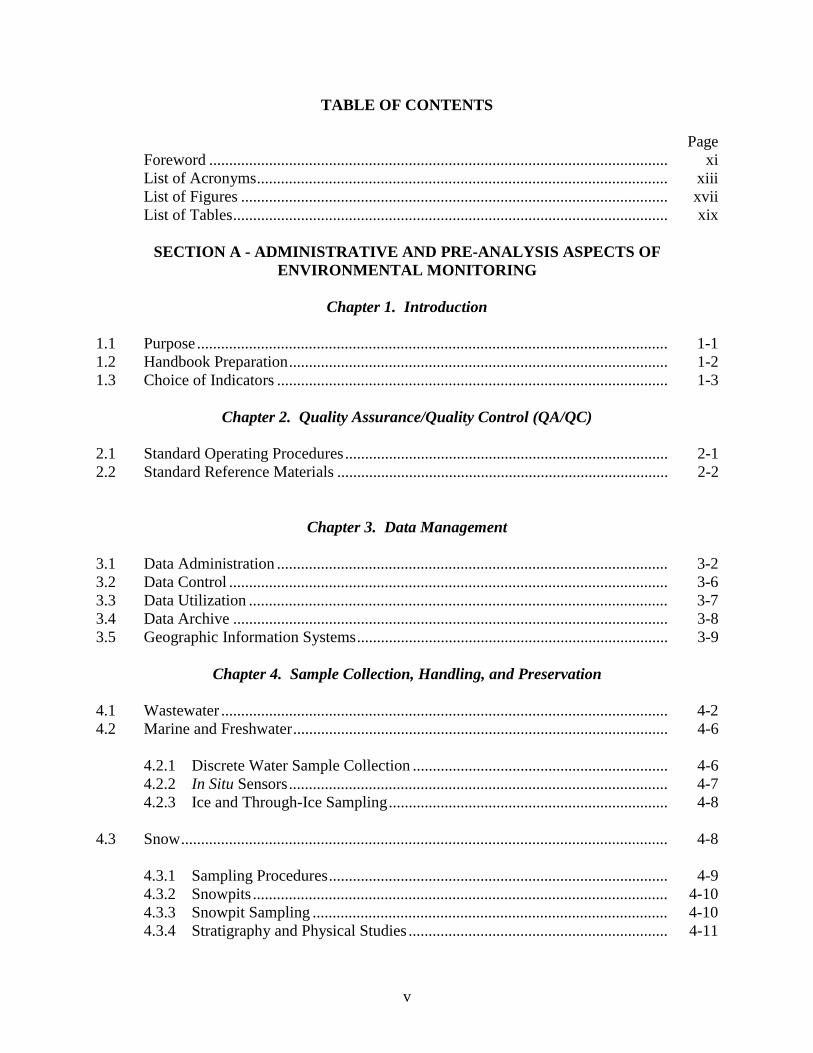
TABLE OF CONTENTS

PageForeword ................................................................................................................... xiList of Acronyms....................................................................................................... xiiiList of Figures ........................................................................................................... xviiList of Tables............................................................................................................. xix

SECTION A - ADMINISTRATIVE AND PRE-ANALYSIS ASPECTS OFENVIRONMENTAL MONITORING

Chapter 1. Introduction

1.1 Purpose ...................................................................................................................... 1-11.2 Handbook Preparation............................................................................................... 1-21.3 Choice of Indicators .................................................................................................. 1-3

Chapter 2. Quality Assurance/Quality Control (QA/QC)

2.1 Standard Operating Procedures................................................................................. 2-12.2 Standard Reference Materials ................................................................................... 2-2

Chapter 3. Data Management

3.1 Data Administration .................................................................................................. 3-23.2 Data Control .............................................................................................................. 3-63.3 Data Utilization ......................................................................................................... 3-73.4 Data Archive ............................................................................................................. 3-83.5 Geographic Information Systems.............................................................................. 3-9

Chapter 4. Sample Collection, Handling, and Preservation

4.1 Wastewater ................................................................................................................ 4-24.2 Marine and Freshwater.............................................................................................. 4-6

4.2.1 Discrete Water Sample Collection ................................................................ 4-64.2.2 In Situ Sensors............................................................................................... 4-74.2.3 Ice and Through-Ice Sampling...................................................................... 4-8

4.3 Snow.......................................................................................................................... 4-8

4.3.1 Sampling Procedures..................................................................................... 4-94.3.2 Snowpits ........................................................................................................ 4-104.3.3 Snowpit Sampling ......................................................................................... 4-104.3.4 Stratigraphy and Physical Studies ................................................................. 4-11

vi

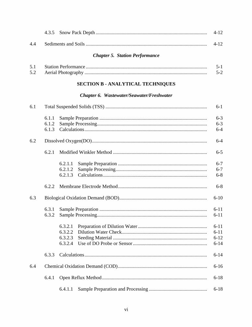
4.3.5 Snow Pack Depth .......................................................................................... 4-12

4.4 Sediments and Soils .................................................................................................. 4-12

Chapter 5. Station Performance

5.1 Station Performance .................................................................................................. 5-15.2 Aerial Photography ................................................................................................... 5-2

SECTION B - ANALYTICAL TECHNIQUES

Chapter 6. Wastewater/Seawater/Freshwater

6.1 Total Suspended Solids (TSS) .................................................................................. 6-1

6.1.1 Sample Preparation ....................................................................................... 6-36.1.2 Sample Processing......................................................................................... 6-36.1.3 Calculations................................................................................................... 6-4

6.2 Dissolved Oxygen(DO)............................................................................................. 6-4

6.2.1 Modified Winkler Method ............................................................................ 6-5

6.2.1.1 Sample Preparation ........................................................................ 6-76.2.1.2 Sample Processing.......................................................................... 6-76.2.1.3 Calculations.................................................................................... 6-8

6.2.2 Membrane Electrode Method........................................................................ 6-8

6.3 Biological Oxidation Demand (BOD)....................................................................... 6-10

6.3.1 Sample Preparation ....................................................................................... 6-116.3.2 Sample Processing......................................................................................... 6-11

6.3.2.1 Preparation of Dilution Water ........................................................ 6-116.3.2.2 Dilution Water Check..................................................................... 6-116.3.2.3 Seeding Material ............................................................................ 6-126.3.2.4 Use of DO Probe or Sensor ............................................................ 6-14

6.3.3 Calculations................................................................................................... 6-14

6.4 Chemical Oxidation Demand (COD)........................................................................ 6-16

6.4.1 Open Reflux Method..................................................................................... 6-18

6.4.1.1 Sample Preparation and Processing ............................................... 6-18

vii

6.4.1.2 Calculations.................................................................................... 6-19

6.4.2 Closed Reflux Method - #1 - Sample Preparation and Processing ............... 6-19

6.4.2.1 Calculations.................................................................................... 6-21

6.4.3 Closed Reflux Method - #2 - Sample Preparation and Processing ............... 6-21

6.4.3.1 Calculations.................................................................................... 6-22

6.5 Acidity....................................................................................................................... 6-22

6.5.1 Sample Preparation and Processing .............................................................. 6-236.5.2 Calculations................................................................................................... 6-23

6.6 pH.............................................................................................................................. 6-24


6.7 Conductivity.............................................................................................................. 6-26


6.8 Nitrate/Nitrite ............................................................................................................ 6-29

6.8.1 Spectrophotometric, Cadmium Reduction Method....................................... 6-29


6.8.2 Autoanalyzer Method.................................................................................... 6-32


6.8.3 Portable Test Kits .......................................................................................... 6-366.8.4 Ion Selective Electrodes ................................................................................ 6-376.8.5 Test Strips...................................................................................................... 6-38

6.9 Phosphate .................................................................................................................. 6-39

6.9.1 Sample Preparation ....................................................................................... 6-40

viii

6.9.2 Sample Processing......................................................................................... 6-416.9.3 Calculations................................................................................................... 6-41

6.10 Temperature (T) ........................................................................................................ 6-416.11 Coliform Bacteria...................................................................................................... 6-42


6.12 Phytoplankton............................................................................................................ 6-46

6.12.1 Sample Preparation ....................................................................................... 6-466.12.2 Sample Processing and Calculations............................................................. 6-476.12.3 Modified Method for Chlorophylls and Carotenoids.................................... 6-49


Chapter 7. Snow

7.1 Metals ........................................................................................................................ 7-1


7.1.1.1 Acid Digestion Procedure for Furnace Atomic Absorption(FAA) Analysis .............................................................................. 7-3

7.1.1.2 Acid Digestion Procedure for ICP and Flame AA Analyses ......... 7-37.1.1.3 Total Metals Sample Preparation Using Microwave Digestion..... 7-3

7.2 Total Petroleum Hydrocarbons ................................................................................. 7-5

7.2.1 Sample Preparation ....................................................................................... 7-67.2.2 Sample Processing......................................................................................... 7-67.2.3 Calculations................................................................................................... 7-7

7.3 Particulates ................................................................................................................ 7-8

7.3.1 Sample Preparation and Processing .............................................................. 7-8

Chapter 8. Soils/Sediments

8.1 Grain Size.................................................................................................................. 8-1

8.1.1 Sample Preparation ....................................................................................... 8-28.1.2 Sample Processing......................................................................................... 8-2

ix

8.1.3 Calculations................................................................................................... 8-4

8.2 Carbon Content ........................................................................................................ 8-4

8.2.1 Total Carbon (TC) ........................................................................................ 8-68.2.2 Total Organic Carbon (TOC) ........................................................................ 8-78.2.3 Total Inorganic Carbon (TIC) ....................................................................... 8-88.2.4 Calculations................................................................................................... 8-8

8.3 Metals ........................................................................................................................ 8-9


8.3.1.1 Acid Digestion Procedure for ICP, Flame AA, and Furnace AAAnalyses ......................................................................................... 8-10

8.3.1.2 Total Metals Sample Preparation Using Microwave Digestion..... 8-128.3.1.3 Total Digestion of Sediment with Hydrofluric Acid for

Trace Metal Analyses..................................................................... 8-15

8.3.2 Graphite Furnace Atomic Absorption Spetrophotometry (GFAAS) ............ 8-168.3.3 Inductively Coupled Plasma Emission Spectroscopy (ICP) ......................... 8-228.3.4 Cold Vapor Atomic Absoprtion Spectroscopy-Mercury (Hg)...................... 8-34

8.3.4.1 Sample Preparation ........................................................................ 8-368.3.4.2 Instrument Analysis........................................................................ 8-36

8.3.5 Calculations................................................................................................... 8-36

8.4 Total Petroleum Hydrocarbons (TPH) ...................................................................... 8-40

8.4.1 Sample Preparation ....................................................................................... 8-408.4.2 Gravimetry .................................................................................................... 8-418.4.3 Infrared Spectrophotometry .......................................................................... 8-418.4.4 Gas Chromatography..................................................................................... 8-42

8.5 Polycyclic Aromatic Hydrocarbons (PAH)............................................................... 8-46

8.5.1 Sample Preparation ....................................................................................... 8-468.5.2 Spectrophotometry ........................................................................................ 8-488.5.3 High Performance Liquid Chromatography (HPLC).................................... 8-568.5.4 Gas Chromatography/Mass Spectrometry (GC/MS) .................................... 8-62

Chapter 9. Bibliography

- Glossary of Terms

FOREWORD

Introduction The development of the Protocol on Environmental Protection to the Antarctic Treaty in

1989, and its accession by Antarctic Treaty Consultative Parties in 1991, intensified the need to implement regular environmental monitoring programs throughout Antarctica. Whilst environmental monitoring has been undertaken in Antarctica over many decades, the Protocol specifically requires regular and effective monitoring of the impacts of activities and verification of predicted impacts.

At its 1994 meeting, the Antarctic Treaty Parties requested COMNAP and SCAR to

conduct technical workshops that would develop an approach to monitoring which would be scientifically sound, practical and cost effective. The outcomes of the two workshops were presented in July 1996 in a report on “Monitoring of Environmental Impacts from Science and Operations in Antarctica”. The report’s conclusions were endorsed by the Treaty Parties and actions subsequently initiated through COMNAP and SCAR towards implementation.

One of the key recommendations was the development of a technical handbook that

would be used as a guide on the scientific protocols for environmental monitoring programs. This handbook has been developed to serve that need and represents the efforts of a large number of individuals to provide an invaluable resource for implementing monitoring programs in Antarctica.

The coordinated effort to define complementary monitoring processes bodes well for

the continued protection of Antarctic resources and values and for minimising human impacts through scientifically sound management of human presence in Antarctica. Acknowledgements

Many individuals contributed to the development of this manual. Special thanks are due to the Project Director, Dr Mahlon C Kennicutt II, who not only managed the development of the handbook but also was deeply involved in organising and participating in the COMNAP/SCAR technical workshops on environmental monitoring.

Several members of the Geochemical and Environment Research Group in the College

of Geosciences A&M University aided in compiling and editing the manual. Drs Guy Denoux, Terry Wade and Jose Sericano assisted in compiling the analytical methods. Ms Dianna Alsup assembled the protocols related to terrestrial monitoring, snow analyses and station activities. Dr Gary Wolff developed the data management sections and aided in production of the manual. Dr Wendy Keeney-Kennicut reviewed the manual for content and accuracy. Ms Debbie Paul was responsible for the typing, editing and final production of the manual.

The manual was greatly improved by the reviews and comments provided by the

COMNAP/SCAR Project Team which was coordinated by Ms Birgit Njastad (Norway) and included Dr Heinz Miller (Germany), Dr Jan-Gunnar Winther (Norway), Dr David Walton (UK) and Dr Joyce Jatko (USA). The manual was also circulated for review and comment to members of the Antarctic Environmental Officers Network (AEON), COMNAP and SCAR. Ms Gillian Wratt Dr Robert H Rutford Chairperson President COMNAP SCAR

xiii

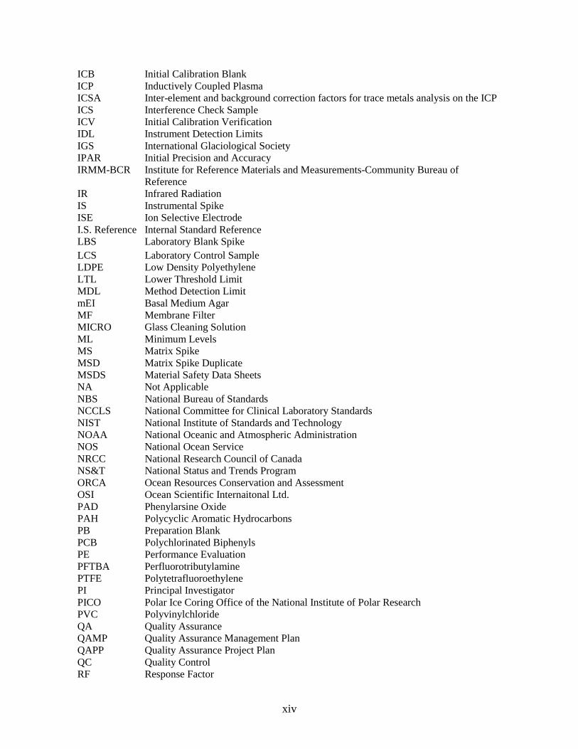
List of Acronyms

AA Auto AnalyzerAAS Atomic Absorption SpectrophotometryACS American Chemical SocietyAEON Antarctic Environmental Officers NetworkAMANDA Antarctic Muon and Neutrino Detector ArrayAMAP Arctic Monitoring and Assessment ProjectAPAC Aromatic Pesticide Analyte CalibrationAPHA American Public Health AssociationASTM American Society for Testing and MaterialsBCR Community Bureau of ReferenceBEA Bile Esculin AgarBHI Brain Heart Infusion broth or agBOD Biological Oxidation DemandCAP College of American PathologistsCCB Continuing Calibration BlankCCV Continuing Calibration Verification standardCD Compact DiskCLP Contract Laboratory Program (EPA)COC Chain of CustodyCOD Chemical Oxidation DemandCOMNAP Council of Managers of National Antarctic ProgramsCRDL Contract Required Detection LimitCRM Certified Reference MaterialsCV Coefficient of VariationCVAAS Cold Vapor Atomic Absorption SpectroscopyDBMS Data Base Management SystemDEM Digital Elevation ModelDI or DIW Deionized WaterDO Dissolved OxygenDUP Sample DuplicateECG Environmental Coordinating GroupEDL Electrodeless Discharge LampEMSL Environmental Monitoring Systems LaboratoryEPA Environmental Protection AgencyEPICA European Project for Ice Coring in AntarcticaFAAS Flame Atomic Absorption SpectrophotometryFAS Ferrous Ammonium SulfateFI Fluorescence IntensityFID Flame Ionization DetectorGBW National Research Center for Certified Reference MaterialsGC Gas ChromatographGC/MS Gas Chromatograph/Mass SpectrometerGFAAS Graphite Furnace Atomic Absorption SpectrophotometryGIS Geographic Information SystemGISP Greenland Ice Sheet ProjectGPS Global Positioning SystemHCL Hollow Cathode LampsHDPE High Density PolyethyleneHPLC High Performance Liquid Chromatography

xiv

ICB Initial Calibration BlankICP Inductively Coupled PlasmaICSA Inter-element and background correction factors for trace metals analysis on the ICPICS Interference Check SampleICV Initial Calibration VerificationIDL Instrument Detection LimitsIGS International Glaciological SocietyIPAR Initial Precision and AccuracyIRMM-BCR Institute for Reference Materials and Measurements-Community Bureau of

ReferenceIR Infrared RadiationIS Instrumental SpikeISE Ion Selective ElectrodeI.S. Reference Internal Standard ReferenceLBS Laboratory Blank SpikeLCS Laboratory Control SampleLDPE Low Density PolyethyleneLTL Lower Threshold LimitMDL Method Detection LimitmEI Basal Medium AgarMF Membrane FilterMICRO Glass Cleaning SolutionML Minimum LevelsMS Matrix SpikeMSD Matrix Spike DuplicateMSDS Material Safety Data SheetsNA Not ApplicableNBS National Bureau of StandardsNCCLS National Committee for Clinical Laboratory StandardsNIST National Institute of Standards and TechnologyNOAA National Oceanic and Atmospheric AdministrationNOS National Ocean ServiceNRCC National Research Council of CanadaNS&T National Status and Trends ProgramORCA Ocean Resources Conservation and AssessmentOSI Ocean Scientific Internaitonal Ltd.PAD Phenylarsine OxidePAH Polycyclic Aromatic HydrocarbonsPB Preparation BlankPCB Polychlorinated BiphenylsPE Performance EvaluationPFTBA PerfluorotributylaminePTFE PolytetrafluoroethylenePI Principal InvestigatorPICO Polar Ice Coring Office of the National Institute of Polar ResearchPVC PolyvinylchlorideQA Quality AssuranceQAMP Quality Assurance Management PlanQAPP Quality Assurance Project PlanQC Quality ControlRF Response Factor

xv

RM Reference MaterialRPD Relative Percent DifferenceRRF Relative Response FactorsRSD Relative Standard DeviationRT Retention TimeSCAR Scientific Committee on Antarctic ResearchSCOR Scientific Committee on Oceanic ResearchSCRC Sagami Chemical Research CenterSIM Selected Ion MonitoringSOPs Standard Operating ProceduresSOW Substitute Ocean WaterSPU Specific Plant UnitSRM Standard Reference MaterialSWE Snow Water EquivalenceT TemperatureTC Total CarbonTCLP Toxicity Characteristic Leaching ProcedureTFE TeflonTIC Total Inorganic CarbonTOC Total Organic CarbonTPH Total Petroleum HydrocarbonsTSS Total Suspended SolidsUNEP United Nations Environment ProgramUNESCO United Nations Educational, Scientific, and Cultural OrganizationUSEPA United States Environmental Protection AgencyUV Ultraviolet

xvii

List of Figures

Page

Figure 3.1 The data management plan............................................................................... 3-2

Figure 3.2 Diagram of data administration tasks............................................................... 3-3

Figure 3.3 Field sample collection label example ............................................................. 3-3

Figure 3.4 Sample collection field form example ............................................................. 3-4

Figure 3.5 Example of Chain of Custody Form ................................................................ 3-5

Figure 3.6 Example of Sample Status Form...................................................................... 3-6

Figure 3.7 Data Control ..................................................................................................... 3-7

Figure 3.8 Data Utilization ................................................................................................ 3-8

Figure 3.9 Data Archive .................................................................................................... 3-8

Figure 3.10 An example GIS composed of data layers of spatial informationregistered to a common map projection ........................................................... 3-10

Figure 6.1 Copper Cadmium Reduction Column.............................................................. 6-33

Figure 6.2 Nitrate-Nitrite Manifold AA-I.......................................................................... 6-35

Figure 6.3 Nitrate-Nitrite Manifold AA-II ........................................................................ 6-35

Figure 8.1 Rayleigh and Raman scatter plus signal to noise ratio..................................... 8-50

Figure 8.2 Synchronous excitation/emission fluorescence spectra of aromatichydrocarbon fractions....................................................................................... 8-53

Figure 8.3 Calibration graph: degraded VMI crude oil 310/360 nm................................. 8-54

xix

List of Tables

PageTable 1.1 Development of a Technical Handbook of Standard Techniques for Use

in Antarctica - Terms of Reference .................................................................. 1-4

Table 1.2 Compilation of Methods Reviewed During the Development of ThisHandbook ......................................................................................................... 1-5

Table 2.1 An Example of the Table of Contents for a Quality Assurance ManagementPlan (QAMP).................................................................................................... 2-4

Table 2.2 An Example of the Table of Contents for a Quality Assurance ProjectPlan (QAPP) for an Individual Project............................................................. 2-5

Table 2.3 Format for an Administrative Standard Operating Procedure (SOP) .............. 2-6

Table 2.4 Format for a Preparation Standard Operating Procedure (SOP) ...................... 2-7

Table 2.5 Format for the Instrument Standard Operating Procedure (SOP) .................... 2-10

Table 2.6 Sources of Standard Reference Materials (SRMs)........................................... 2-14

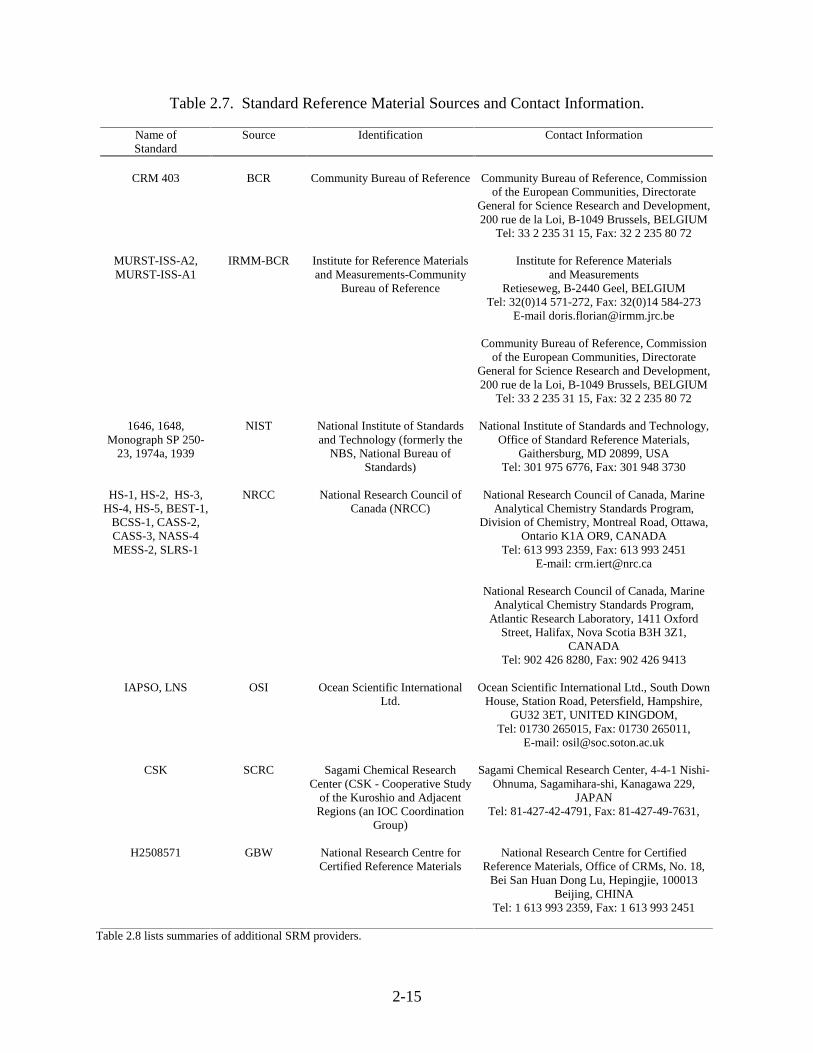
Table 2.7 Reference Materials by Matrix and Analyte .................................................... 2-15

Table 2.8 Summary of Standard Reference Material Providers....................................... 2-16

Table 2.9 Website Listing for Methods and Other References ........................................ 2-18

Table 4.1 The Advantages and Disadvantages of Manual and Automatic Samplingof Wastewaters ................................................................................................. 4-3

Table 4.2 Summary of Preservation and Holding Times ................................................. 4-4

Table 4.3 Drill Types........................................................................................................ 4-9

Table 8.1 Wavelength Used for Routine ICP Quantitative Trace Metal Analytes .......... 8-23

Table 8.2 Calibration Standard Concentration ................................................................. 8-24

Table 8.3 Check 2 Standard Concentration...................................................................... 8-26

Table 8.4 Key Elements of ICP Quality Control.............................................................. 8-26

Table 8.5 Typical Analytical Protocol Operating Parameters for the Modified ScottSpray Chamber................................................................................................. 8-29

xx

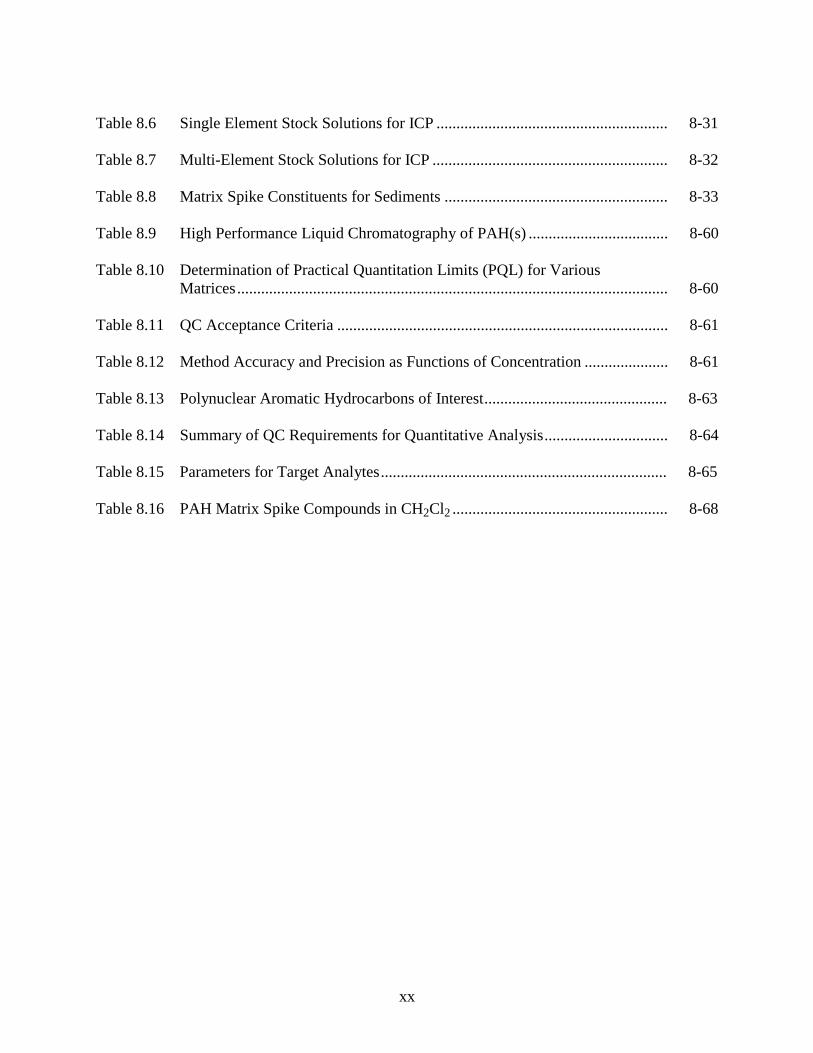
Table 8.6 Single Element Stock Solutions for ICP .......................................................... 8-31

Table 8.7 Multi-Element Stock Solutions for ICP ........................................................... 8-32

Table 8.8 Matrix Spike Constituents for Sediments ........................................................ 8-33

Table 8.9 High Performance Liquid Chromatography of PAH(s) ................................... 8-60

Table 8.10 Determination of Practical Quantitation Limits (PQL) for VariousMatrices............................................................................................................ 8-60

Table 8.11 QC Acceptance Criteria ................................................................................... 8-61

Table 8.12 Method Accuracy and Precision as Functions of Concentration ..................... 8-61

Table 8.13 Polynuclear Aromatic Hydrocarbons of Interest.............................................. 8-63

Table 8.14 Summary of QC Requirements for Quantitative Analysis............................... 8-64

Table 8.15 Parameters for Target Analytes........................................................................ 8-65

Table 8.16 PAH Matrix Spike Compounds in CH2Cl2 ...................................................... 8-68

SECTION A

ADMINISTRATIVE AND PRE-ANALYSIS ASPECTSOF ENVIRONMENTAL MONITORING

1-1

CHAPTER 1.INTRODUCTION

This handbook provides guidance on standard techniques and methodologies for a firsttier of indicators for monitoring programs in Antarctica. The handbook is intended to encouragegreater comparability of results across the wide spectrum of activities conducted under theauspices of monitoring as required by the Protocol on Environmental Protection to the AntarcticTreaty. Adoption of common techniques increases the value of monitoring activities byencouraging the collection of comparable data by all Treaty countries. Intercomparability willfacilitate continent-wide interpretation of monitoring results allowing each program to benefitfrom others’ experiences. While recommended methods are detailed, alternative methods maybe appropriate as long as data of known quality is produced. While the approach is to adhere toreliable and intercomparable methodologies, any data produced under strict quality assuranceguidelines will provide the needed information to managers of national Antarctic programs forsound, effective scientific-based decision making.

1.1 Purpose

In July 1996, the Scientific Committee on Antarctic Research (SCAR) and the Council ofManagers of National Antarctic Programs (COMNAP) published the results of two workshopsentitled “Monitoring of Environmental Impacts from Science and Operations in Antarctica”(Kennicutt et al. 1996). A wide range of issues related to monitoring in Antarctica wereaddressed in the report. The workshop recommended that a technical handbook of standardizedmethods be prepared for the key environmental indicators identified by the workshop.COMNAP subsequently developed the Terms of Reference for the work (Table 1.1). Thefollowing handbook was produced in response to this mandate and its content has been reviewedby a Project Team consisting of two members of the Antarctic Environmental Officers Network(AEON) of COMNAP, the chair of the COMNAP Environmental Coordinating Group (ECG),and a SCAR representative.

The intent of this handbook is to provide guidance for the measurement of a first tier ofindicators that are most relevant to monitoring impacts due to scientific stations and theassociated support activities. The mandate is also to provide methods that are relatively simpleand cost-effective given the limited resources that most national Antarctic programs have formonitoring activities. Within this context, it is also important that monitoring provide relevantand unambiguous information to support sound management decisions at Antarctic stations.

In most instances, well-tested and proven techniques and methodologies that are routinelyused in monitoring programs world-wide were selected for inclusion in the handbook. Asmonitoring efforts develop in Antarctica, more definitive methods may be needed to answer themore complex issues faced by managers of national Antarctic programs. In many cases, anassessment of the current status of the system can be made utilizing the techniques detailed inthis handbook. The data generated can be used to indicate whether more extensive investigationor additional directed monitoring is needed. The methods proposed provide a first orderestimation of the status and changes in the quality of the environment at scientific stations.

1-2

In the coming years as data is collected and experience is gained, it will be important toreview and revise the suggested methods to ensure they adequately meet the aims of monitoring.Advances in technologies and methodologies should also be adopted as techniques are improved.Other acceptable methods, that give comparable information, may also be added to the currentcompendium of methods as appropriate. In addition, as baseline information is collected it maybecome apparent that other portions of the system or other influencing factors or agents need tobe measured to more fully understand and interpret monitoring results. As mentioned, morecomplex questions directly related to deterioration or change in the more visible resources andvalues of the Antarctic continent, in particular the wildlife, may warrant the adoption of methodsmore directly indicative of biological effects. Biology based measurements will need to becarefully considered in light of the magnitude of natural variability in biological communities inAntarctica and the long timeframes over which change occurs. However, certain biology-basedmeasurements such as change in community structure, biological uptake of contaminants,production of metabolites, and more subtle indicators of stress in organisms and communitiesmay be appropriate indicators for monitoring programs. While an ideal monitoring programwould include direct measurement of the relevant attributes of biological resources, manychallenges still remain in perfecting biology-based indicators. Research is needed to develop abetter understanding of the time frames of biological changes, the extent and nature of naturalvariability in important populations, and the linkages between biological responses and causativeagents. Until these complex questions can be resolved, direct monitoring of biological resourceswill be of limited use in developing management strategies in Antarctica.

This manual should be updated and amended on an as needed basis. The methods can berevised or replaced when sufficient information is available to justify a revision. This manual isintended to encourage synergy amongst the ever-growing number of monitoring programs inAntarctica by providing for the collection of comparable data.

1.2 Handbook Preparation

In preparing this handbook, a variety of sources of information were consulted (Table1.2). Scientific protocols already being used were the “methods of choice” including thoseproven useful in monitoring programs world-wide. Methods of demonstrated accuracy andprecision through testing and intercalibration were preferred. The methods of the ArcticMonitoring and Assessment Project (AMAP) were of special interest. However, AMAPmethods are targeted for regions that contain significant human populations and have relativelyhigh levels of contamination that are not expected to be encountered in Antarctica. Theinformation compiled by COMNAP's “Summary of Environmental Activities in Antarctica,1998” was used to evaluate practices that are already in place and their performance to date.Contributors to the COMNAP summary and others were canvassed to develop furtherinformation related to the methods used and to incorporate the experiences gained from theapplication of monitoring methods in Antarctica. The conclusions from all relevant COMNAPand SCAR workshops were taken into account with special attention paid to the 1996 workshopreport (Kennicutt et al. 1996).

1-3

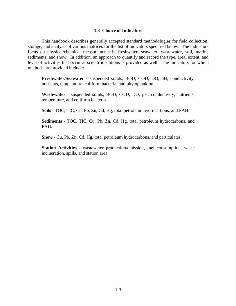
1.3 Choice of Indicators

This handbook describes generally accepted standard methodologies for field collection,storage, and analysis of various matrices for the list of indicators specified below. The indicatorsfocus on physical/chemical measurements in freshwater, seawater, wastewater, soil, marinesediments, and snow. In addition, an approach to quantify and record the type, areal extent, andlevel of activities that occur at scientific stations is provided as well. The indicators for whichmethods are provided include:

Freshwater/Seawater - suspended solids, BOD, COD, DO, pH, conductivity,nutrients, temperature, coliform bacteria, and phytoplankton.

Wastewater - suspended solids, BOD, COD, DO, pH, conductivity, nutrients,temperature, and coliform bacteria.

Soils - TOC, TIC, Cu, Pb, Zn, Cd, Hg, total petroleum hydrocarbons, and PAH.

Sediments - TOC, TIC, Cu, Pb, Zn, Cd, Hg, total petroleum hydrocarbons, andPAH.

Snow - Cu, Pb, Zn, Cd, Hg, total petroleum hydrocarbons, and particulates.

Station Activities - wastewater production/emission, fuel consumption, wasteincineration, spills, and station area.

1-4

Table 1.1 Development of a Technical Handbook of Standardized Techniques for Use inAntarctica - Terms of Reference.

Terms of Reference

1. To prepare a technical handbook of standardized monitoring methodologies for a common setof indicators for use by national Antarctic programs and other Antarctic operations, formonitoring the impact of science and operations activities in Antarctica in order to comply withthe Protocol requirements for monitoring.

2. The priority for the first edition of the handbook will be methodologies for monitoring theimpacts of stations in Antarctica.

3. The handbook will include:

• standardized techniques and methodologies for monitoring the principal physical andchemical indicators identified in the SCAR/COMNAP report, 1996 (“Monitoring theEnvironmental Impacts from Science and Operations in Antarctica”, Kennicutt et al.1996);

• standardized techniques and methodologies for biological monitoring based on therecommended options identified in the SCAR/COMNAP report 1996;

• guidelines for data management related to monitoring programs.

4. In preparing the handbook, the following shall be taken into account:

• scientific protocols which already exist for monitoring the indicators identified(including those used outside Antarctica);

• experience gained and information available through existing Antarctic monitoringactivities (refer in particular to the COMNAP document “Summary of EnvironmentalMonitoring Activities in Antarctica”, Kennicutt et al. May 1998);

• relevant conclusions set out in the SCAR/COMNAP report 1996; and

• mechanisms to update monitoring techniques and to extend the contents of thehandbook.

1-5

Table 1.2. Compilation of Methods Reviewed During the Development of this Handbook(EPA-U.S. Environmental Protection Agency, ASTM-American Society for TestingMaterials, NOAA NS&T-National Oceanic and Atmospheric AdministrationNational Status and Trends Mussel Watch Program, APHA-American PublicHealth Association).

Analyte Method Description Source Matrix

Acidity EPA 305.1 Titrimetric EPA water, wastewaterEPA 305.2 Titrimetric EPA water

Aromatics ASTM D5831-96 Screening for fuels ASTM soilsEPA 602 Purge and Trap gas

chromatographicEPA surface, sea,

wastewaters, soils,sediments, sludges

(PAH) EPA 550, 550.1 Liquid-Liquid extraction withHPLC, Coupled Ultraviolet and

Fluorescence Detection

EPA water

EPA 3540, NOSORCA 130

Soxhlet extraction withdichloromethane

EPA,NOAANS&T

soils, sediments

NOS ORCA 130 Extraction with dichloromethanewith tissumizer; Kuderna-Danish

technique

NOAANS&T

Tissues

PCB, PAH, TPH Mudroch et al.(1997)

Recommended extractionprocedures

sediment

Hydrocarbons EPA 5030, 5030a,5030b

Purge and Trap EPA water, wastewater

EPA 8015, 8015a,8015b

Gas Chromatography EPA water, wastewater

NOS ORCA 130 Gas Chromatography/MassSpectrometry--selected ion

monitoring

NOAANS&T

water, sediments, tissue

(Volatiles) ASTM D4547-91 Sampling for volatile organics ASTM soils, sediments, wastes

BOD EPA 405.1 Incubation, Probe EPA water

Characterization ASTM D2488-93 Visual identification anddescription

ASTM soils

COD EPA 410.1 Titrimetric EPA waterEPA 410.2 Titrimetric EPA saline watersEPA 410.3 Titrimetric EPA waterEPA 410.4 Titrimetric EPA ground, surface waters

APHA 5220b Open Reflux method APHA water, wastewaterAPHA 5220c, d Closed Reflux method APHA water, wastewater

DO 360.1 Probe EPA water--outfalls, streams360.1 Titration, Probe EPA water, wastewater

Cadmium (Cd) EPA 213.2 CLP Atomic absorption, furnacetechnique

EPA water, wastewater

1-6

Table 1.2. (Cont.)


Coliform EPA 1600 Membrane Filter Test EPA water, wastewater

Copper (Cu) EPA 220.2 CLP Atomic absorption, furnacetechnique

EPA

DecontaminationProcedures

ASTM D5088 Field equipment (nonradioactivesites)

ASTM soils, sediments,sludges, wastes

Dry Weight NOS ORCA 130 Dry weight NOAANS&T

sediments

NOS ORCA 130 Dry weight NOAANS&T

Tissues

Grain size ASTM D2217-85 Wet preparation, particle sizeanalysis

ASTM soils

ASTM D2217-85 Dry preparation, particle sizeanalysis

ASTM soils

NOS ORCA 130 Pipette Method NOAANS&T

sediment

Lead (Pb) ASTM E 1727-95 Atomic spectrometry ASTM soilsEPA 239.2 CLP Atomic absorption, furnace

techniqueEPA

Mercury (Hg) EPA 245.1 Cold Vapor Atomic AbsorptionSpectrometry

EPA ground, surface,wastewaters

EPA 245.3 Inorganic Hg detection usingHPLC with ECD

EPA ground, surface,wastewaters

EPA 245.5 Cold Vapor Atomic AbsorptionSpectrometry

EPA Soils, sediments, bottomdeposits, sludge

EPA 245.6 Cold Vapor Atomic AbsorptionSpectrometry

EPA Tissues

Metals and TraceElements

EPA 200.7,Mudroch et al.

(1997)

Inductive Coupled Plasma -Atomic Emission

EPA water, wastewaters,solid wastes

Mudroch et al.(1997)

Inductive Coupled Plasma - MassSpectrometry

sediment


Decomposition Technique sediment


Flame Atomic AbsorptionSpectrometry

sediment

1-7

Table 1.2. (Cont.)


Metals and TraceElements


Quartz Tube Atomic AbsorptionSpectrometry

sediment


Graphite Furnace AtomicAbsorption Spectrometry

sediment


Slurry Atomic AbsorptionSpectrometry

sediment

Nitrate (NO3) EPA 352.1 Colorimetric, Brucine EPA surface, sea,wastewaters

EPA 353.1 Colorimetric, Automated,Hydrazine Reduction

EPA surface, sea,wastewaters

EPA 353.2 Automated Colorimetry EPA surface, sea,wastewaters

C and P also Mudroch et al.(1997)

Dry Combustion, Filter, Kjeldahletc.

sediment

Nitrite EPA 353.1 Colorimetric, Automated,Hydrazine Reduction


EPA 353.2 Automated Colorimetry EPA surface, sea,wastewaters

C and P also Mudroch et al.(1997)

Dry Combustion, Filter,Kjeldahl etc.

sediment

pH ASTM D 4972-95 Paper ASTM soilsEPA 150.1 Electrometric EPA wastewatersEPA 9040,

9040A, 9040BElectrometric EPA wastewaters

EPA 9041, 9041A Electrometric EPA wastewatersEPA 9045,

9045A, 9045B,9045C

Electrometric EPA soils, waste, sludge


General information sediment

Sample Preparation Mudroch et al.(1997)

Collection, Storage, Analysis sediment

Snow Clarke and Noon(1985)

Nucleopore filter, photometer Particulate matter (pm)

Clarke and Noon(1988)

Collection, Nucleopore filters Particulate matter (pm)-elemental carbon

Chylek et al.(1987)

Collection, Quartz and PolyvinylMembrane Filtration,

Particulate matter (pm)

Chylek et al.(1983)

Snow Albedo Model Snow Cover

Stein et al.(1996)

Time domain reflectometry,freezing calorimetry technique

Snow dry density, liquidwater content

1-8

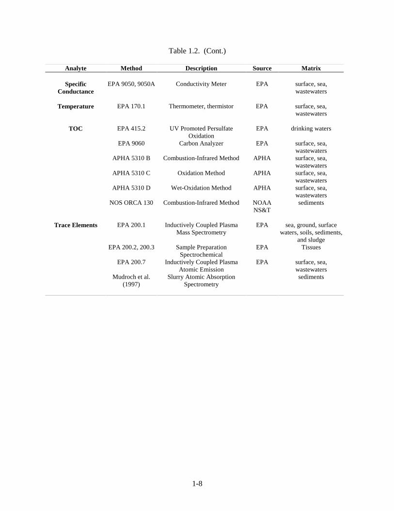
Table 1.2. (Cont.)


SpecificConductance

EPA 9050, 9050A Conductivity Meter EPA surface, sea,wastewaters

Temperature EPA 170.1 Thermometer, thermistor EPA surface, sea,wastewaters

TOC EPA 415.2 UV Promoted PersulfateOxidation

EPA drinking waters

EPA 9060 Carbon Analyzer EPA surface, sea,wastewaters

APHA 5310 B Combustion-Infrared Method APHA surface, sea,wastewaters

APHA 5310 C Oxidation Method APHA surface, sea,wastewaters

APHA 5310 D Wet-Oxidation Method APHA surface, sea,wastewaters

NOS ORCA 130 Combustion-Infrared Method NOAANS&T

sediments

Trace Elements EPA 200.1 Inductively Coupled PlasmaMass Spectrometry

EPA sea, ground, surfacewaters, soils, sediments,

and sludgeEPA 200.2, 200.3 Sample Preparation

SpectrochemicalEPA Tissues

EPA 200.7 Inductively Coupled PlasmaAtomic Emission



Slurry Atomic AbsorptionSpectrometry

sediments

2-1

CHAPTER 2.QUALITY ASSURANCE/QUALITY CONTROL (QA/QC)

Quality assurance (QA) involves all of the planned and systematic actions necessary toprovide confidence that the work performed conforms to the monitoring program’s goals.Quality assurance encompasses quality control (QC) which involves the examination of workperformed in the context of the standards agreed upon for the measurements being made.Quality assurance is particularly important to Antarctic monitoring in that each country will bepursuing its own program. In order to promote synergy and cooperation, comparable data mustbe collected. The basis for this cooperation will be the production of data of known quality.This combining of efforts will allow national programs to benefit from the experiences of othermanagers of national Antarctic programs. The same activities occur at most scientific stationseven though the intensity, duration, frequency, and mixture of activities varies widely. QA isalso key to detecting human induced change in areas where natural variability is expected to behigh. Many impacts may be subtle and long-term reliable data collection will be needed todetect and respond to changes caused by human activities.

As a first step, an atmosphere that encourages and requires adherence to QA/QCprinciples must be provided. Management is responsible for ensuring that adequate resources areavailable to implement the QA/QC system thus assuring the quality of the data produced. Theformal recognition of quality goals ensures that monitoring goals are met and that those involvedin monitoring are committed to providing the highest quality performance.

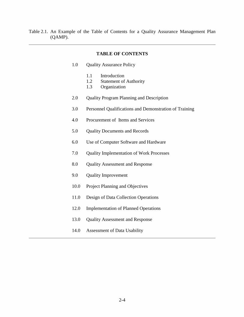
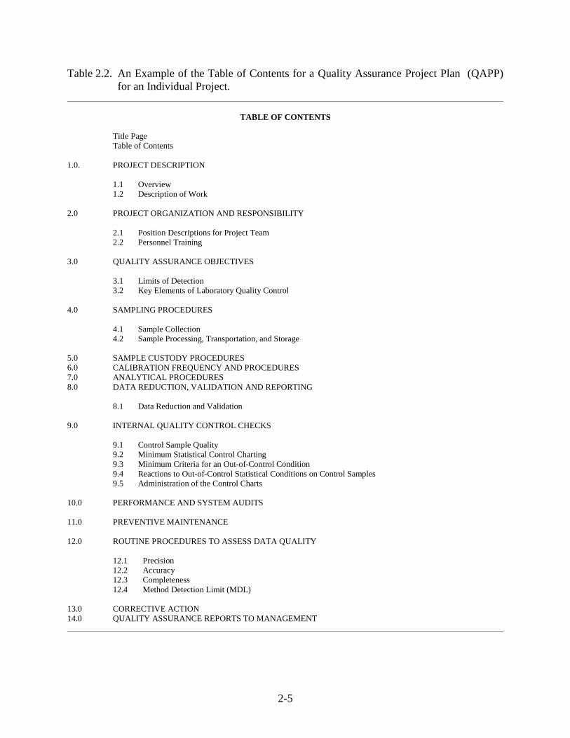
Monitoring programs should be conducted based on a detailed written plan. This plancan take the form of a Quality Assurance Management Plan (QAMP), Quality Assurance ProjectPlan (QAPP), or other planning documents. A QAMP or QAPP details the critical elements of amonitoring program (Tables 2.1 and 2.2).

The level of documentation that is needed for a specific monitoring program will dependon the complexity of the program and the resources available. A written explanation of the goalsand the procedures of the program are essential for continuity and for communicating monitoringresults to others. A formal QAMP or QAPP may not be necessary, but some type ofdocumentation of the details of the program are recommended. Those program elements that areimportant for future reference and for others to judge the quality of the results produced areillustrated in the attached QAMP and QAPP Table of Contents (Tables 2.1 and 2.2). This is oneapproach and each program can decide what documentation is most appropriate to their program.These documents are also important in training new personnel and ensuring that all involvedhave a common understanding of the program’s goals. If external contractors are utilized for anyportion of the project, they should be required to produce similar quality assurance documentsthat are in concert with the program’s goals.

2.1 Standard Operating Procedures

While this technical handbook includes sufficient details for the conduct of variousmethodologies and techniques, it is recommended that each program adapt the guidelines to theirspecific needs. It is also recommended that the analyst refer to the original methodological

2-2

references for greater detail. In order to develop procedures that are specific to each laboratoryand the instrumentation available, more detailed Standard Operating Procedures (SOPs) shouldbe developed by each monitoring program to ensure long-term intercomparability of results.Procedures should be updated on a regular basis to provide revised and improved techniquesbased on hands-on experience. SOPs also facilitate the transfer of knowledge when multipleanalysts are involved or monitoring occurs over many years.

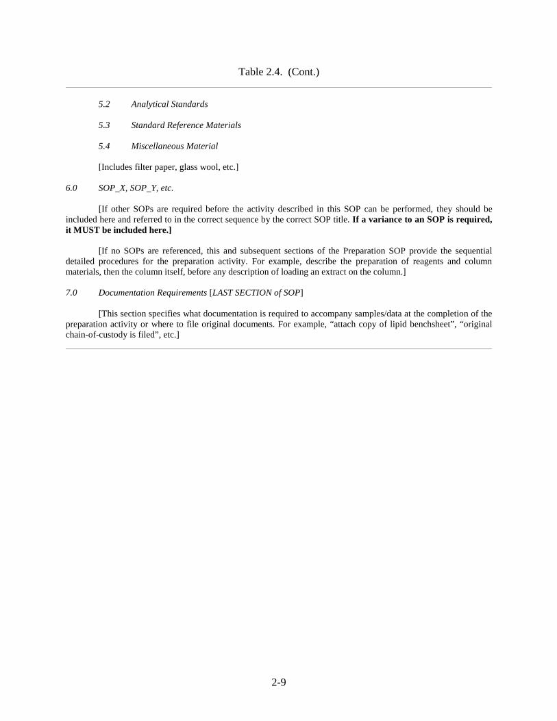
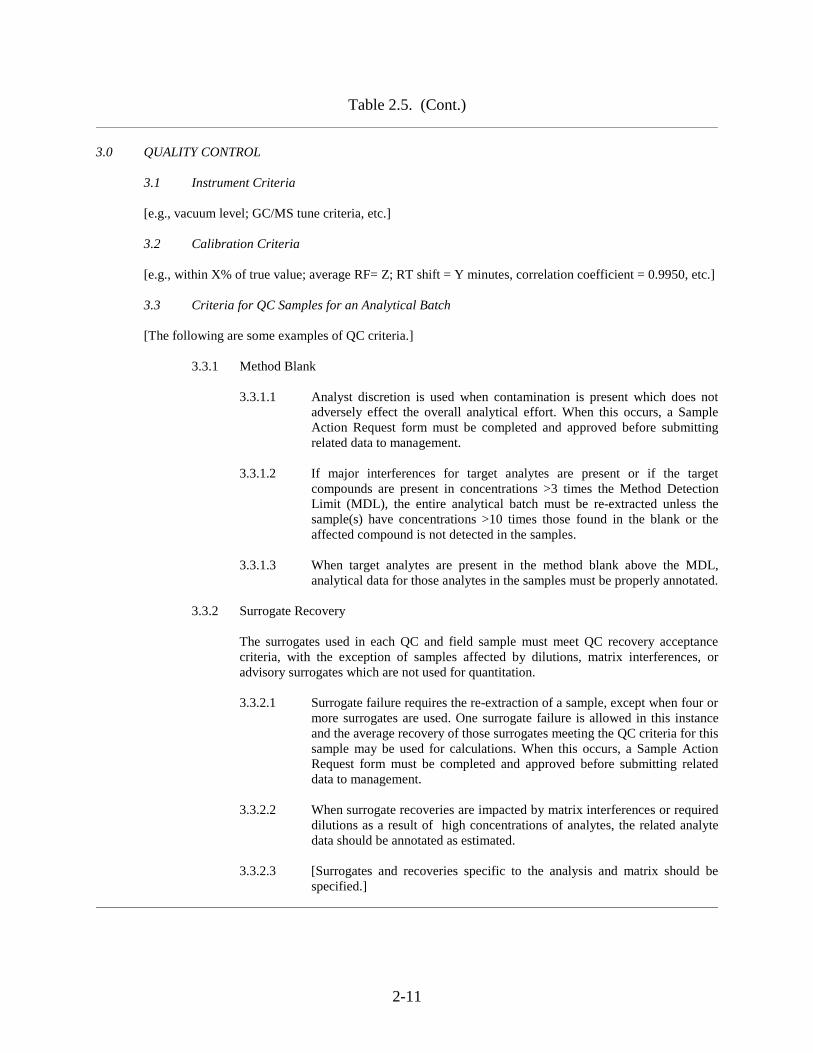
A procedure should be established for developing new or modifying existing StandardOperating Procedures. SOPs should use standardized formats, be subject to a review process,and provide for management approval. The need to modify SOPs may occur as a result of theintroduction of new or improved field or analytical techniques or modification of projectobjectives or goals. A person should be designated to review, coordinate, and prepare new orrevise current Standard Operating Procedures. All who use the SOPs should be encouraged toprovide suggestions and observations regarding the performance of the SOP. However,alteration of the SOP requires formal review and approval to maintain comparability amongstmeasurements. Appropriate testing should be performed to ensure that equivalent data isproduced by any revised or new SOP. Suggested formats for three types of SOPs are provided:administrative, preparation and instrumental procedures (Tables 2.3-2.5).

One important component of an SOP is explicit identification of any specific hazard thatthe field team or analyst might be exposed to, especially solvents and chemicals. This shouldinclude any specific handling requirements and precautions that should be taken. In addition,clear guidance on the disposal of any hazardous waste should also be included.

Any laboratories contracted to perform analyses should be requested to prepare andsubmit SOPs for review and approval before the initiation of any analyses.

2.2 Standard Reference Materials

Reference materials are key to Antarctic monitoring where results will be produced bymany independent programs. The routine analysis of reference materials provides a benchmarkor reference for comparison of data amongst laboratories. Any bias or artifact in results will bedocumented from the results of laboratories analyzing the same material or material havingconstituents of an agreed value. Reference materials are important for the internal assessment ofmethodological performance as well.

Standard Reference Materials(SRMs) are used by laboratories to validate their analyticalmethods and assess accuracy. If Certified Reference Materials (CRMs) with knownconcentrations are not available, reference materials with information values can be substituted.The term standard reference material (SRM) is used to indicate either CRMs or other RMs.After validation, methods are monitored to verify that they continue to produce acceptable dataand meet quality assurance objectives. The SRM matrix and analyte concentrations used shouldbe a reasonable match to that of the samples being analyzed. It may be difficult to find SRMsthat meet all of the matrix and concentration requirements, therefore compromises are inevitable.However, the availability of SRMs has greatly increased in recent years and their use is the bestavailable approach for the determination of precision and accuracy (Tables 2.6-2.8).

2-3

SRMs have undergone extensive testing to ensure a homogeneous sample for replicateanalyses to determine the precision and accuracy of a method. To calculate a standard deviationwhen validating a method, the minimum number of analyses is three. The resulting mean andstandard deviation can then be compared to the certified or information values provided with theSRM.

The SRM is analyzed as if it were a sample using the standard analytical protocols. It isdesirable to analyze the SRM as a blind test (the analyst is unaware that the sample is an SRM)to ensure that it receives no special handling or treatment. Acceptable limits should be set forSRM results based on the program’s goals. The measurements may have an adequate precision(an acceptable standard deviation), but the results do not agree with the reported concentration.This is caused by a bias in the method. The method should be improved to eliminate the bias ifpossible or an alternative method should be chosen.

If the analyses of the SRM shows the method to have acceptable accuracy for the goals ofthe monitoring, then analyses of actual samples can proceed. The RM should be reanalyzedfrequently to confirm that the method performance meets the QC criteria. Whenever the SRManalysis shows that the desired method accuracy is not being met, the affected sample sets arereanalyzed. It is also necessary to determine the cause of the failure and correct it. If thefrequent use of SRMs is cost prohibitive, a secondary laboratory reference material, producedwithin the laboratory, can be used after standardization against the SRM. Like SRMs, thissecondary material should be homogeneous to provide consistent results. A summary of relevantSRMs, and their sources, are provided in Tables 2.6-2.9.

If a contract laboratory is used, the frequency of analysis of SRMs should be stipulated.It is also a good practice for the organization submitting samples for analysis to intersperseSRMs as blind checks on performance.

An additional check on interlaboratory comparability is the provision of either a commonsample for analysis by all laboratories (“round-robin intercomparisons”) or the exchange ofsamples between laboratories. These types of exercises often require independent organizationof the exercise to assure anonymity of the participants and full disclosure of the results. Thereare a range of organizations that support and facilitate these independent intercomparisons for awide range of analytes. Participation in intercalibrations should be encouraged. In someinstances, a subset of samples (i.e., 10%) is sent to a second laboratory to serve as a QA/QCcheck and to confirm of the quality of the data being produced.

2-4

Table 2.1. An Example of the Table of Contents for a Quality Assurance Management Plan(QAMP).

TABLE OF CONTENTS

1.0 Quality Assurance Policy

1.1 Introduction1.2 Statement of Authority1.3 Organization

2.0 Quality Program Planning and Description

3.0 Personnel Qualifications and Demonstration of Training

4.0 Procurement of Items and Services

5.0 Quality Documents and Records

6.0 Use of Computer Software and Hardware

7.0 Quality Implementation of Work Processes

8.0 Quality Assessment and Response

9.0 Quality Improvement

10.0 Project Planning and Objectives

11.0 Design of Data Collection Operations

12.0 Implementation of Planned Operations

13.0 Quality Assessment and Response

14.0 Assessment of Data Usability

2-5

Table 2.2. An Example of the Table of Contents for a Quality Assurance Project Plan (QAPP)for an Individual Project.

TABLE OF CONTENTS

Title PageTable of Contents

1.0. PROJECT DESCRIPTION

1.1 Overview1.2 Description of Work

2.0 PROJECT ORGANIZATION AND RESPONSIBILITY

2.1 Position Descriptions for Project Team2.2 Personnel Training

3.0 QUALITY ASSURANCE OBJECTIVES

3.1 Limits of Detection3.2 Key Elements of Laboratory Quality Control

4.0 SAMPLING PROCEDURES

4.1 Sample Collection4.2 Sample Processing, Transportation, and Storage

5.0 SAMPLE CUSTODY PROCEDURES6.0 CALIBRATION FREQUENCY AND PROCEDURES7.0 ANALYTICAL PROCEDURES8.0 DATA REDUCTION, VALIDATION AND REPORTING

8.1 Data Reduction and Validation

9.0 INTERNAL QUALITY CONTROL CHECKS

9.1 Control Sample Quality9.2 Minimum Statistical Control Charting9.3 Minimum Criteria for an Out-of-Control Condition9.4 Reactions to Out-of-Control Statistical Conditions on Control Samples9.5 Administration of the Control Charts

10.0 PERFORMANCE AND SYSTEM AUDITS

11.0 PREVENTIVE MAINTENANCE

12.0 ROUTINE PROCEDURES TO ASSESS DATA QUALITY

12.1 Precision12.2 Accuracy12.3 Completeness12.4 Method Detection Limit (MDL)

13.0 CORRECTIVE ACTION14.0 QUALITY ASSURANCE REPORTS TO MANAGEMENT

2-6

Table 2.3. Format for an Administrative Standard Operating Procedure (SOP).

The following format is for an Administrative SOP and presents an outline for the general requirements forrepetitive administrative or documentation activities. This outline is a suggested format, although the wordingshould be modified to reflect the content and applicability of each Administrative SOP.

1.0 PURPOSE

1.1 Summary

This procedure [establishes the selection and training requirements] for personnel involved in theoperation, maintenance, and technical support of the monitoring programs.

1.2 Application

The provisions of this SOP apply to all operations, staff, and management.

2.0 SAFETY

The hazards, toxicity or carcinogenicity of each compound or reagent used in standard operatingprocedures have not been precisely determined. However, each chemical compound should be treated as apotential health hazard. Exposure to these compounds should be reduced to the lowest possible level. Thelaboratory maintains Material Safety Data Sheets (MSDS) which contain information regarding the safe handling ofchemicals. A reference file of MSDS is available to all personnel involved with these materials. All laboratorypersonnel should direct any questions regarding safety issues to their supervisors or the Safety Officer. [This is aU.S. requirement.]

3.0 RESPONSIBILITIES AND AUTHORITIES

4.0 PERSONNEL SELECTION

5.0 TRAINING

5.1 Requirements

5.2 Primary Training

5.3 Supplemental Training

5.4 Continuing Training

6.0 Record Requirements

2-7

Table 2.4. Format for a Preparation Standard Operating Procedure (SOP).

A preparation SOP provides detailed procedures for field activities, describing the collection and handlingof samples prior to analysis, and also delineates the steps required for the preparation of a sample for the appropriateanalytical or instrumental activity. The procedures described in these SOPs ensure the sample’s representativeness,non-contamination, and appropriate handling and storage.

The outline below provides suggested elements for this type of SOP. When appropriate, sections may beadded, omitted, or modified, or the abbreviation “NA” (not applicable) may be used.

1.0 PURPOSE

This document provides the procedures (sample collection, field analysis, sample extraction, sample extractpurification, etc.) that are to be used in monitoring programs.

1.1 SUMMARY OF METHOD

[This section provides a BRIEF summary of the preparation activity. This section can concisely referenceother SOPs (by topic) which must be used in addition to the procedure described in this SOP. A more detaileddescription of such additional SOPs, including any required variances can be included later in this document.]

1.2 APPLICABILITY

1.2.1 Matrix

[This section specifies general matrices in sentence format such as biological tissue,soil/sediment, water, or may be highly specific, such as “lichens only” or may be NA forcertain field procedure such as launching and recovery of sensors.]

1.2.2 Interferences

[Typically this section may state either NA or the statements similar to the followingwhich are relevant to sample preparation:

“High purity reagents and solvents must be used, and all equipment and glassware mustbe scrupulously cleaned. Laboratory method blanks must be prepared for analysis todemonstrate the lack of contamination during preparation activities that would interferewith the measurement of the target analytes. Gloves, certain plastic components, andcertain greases must not be used if these will result in phthalate contamination.”

“Column or gel permeation chromatographic procedures are used to remove undesiredco-extracted interfering components; these procedures must be performed carefully tominimize loss of target analytes. Gloves, other plastic components, and certain greasesmust not be used if these will result in phthalate contamination.”]

“Trip or field blanks may be a specified QA/QC component. This section should alsospecify any protocols for handling and disposal of hazardous waste materals.”

1.2.3 Special Precautions

[This section may omitted or may specify precautions which are pertinent to thepreparation activity. It may refer to “Normal laboratory (or field) safety procedure...”, ormay contain special information from the MSDS for specific hazards or informationregarding areas such as a “Caution: open samples in a biological safety cabinet”; or itmay provide directions such as “Sample upstream of diesel fumes”.]

2-8

Table 2.4. (Cont.)

1.2.4 Reporting Units

[When the Preparation SOP provides reportable data for a project, this section shouldspecify the required reporting units, on both matrix specific and wet weight versus dryweight basis. This section may also be omitted or an NA is used when appropriate.]

1.2.5 Method Detection Limits (MDL)

[If applicable, use of tabular MDL information on a separate sheet will aid in futureupdates for the SOP. This section can refer to the MDL information in the InstrumentalSOP.]

2.0 SAFETY

The hazards, toxicity or carcinogenicity of each compound or reagent used in standard operatingprocedures have not been precisely determined. However, each chemical compound should be treated as a potentialhealth hazard. Exposure to these compounds should be reduced to the lowest possible level. The laboratorymaintains Material Safety Data Sheets (MSDS) which contain information regarding the safe handling of chemicals.A reference file of MSDS is available to all personnel involved with these materials. All laboratory personnelshould direct any questions regarding safety issues to their supervisors or the Safety Officer. [A U.S. requirement.]

3.0 QUALITY CONTROL REQUIREMENTS

[This section typically provides a numbered list with a definition and summary description of standard QC(i.e., preparation of a method blank; preparation of the MS/MSD per 20 samples or less, etc.) and includesapplicable QC acceptance criteria for the preparation activity. QC criteria typically would include RPD calculationsand any calibration requirements. Note that this section should indicate that QC criteria for analytical results areaddressed in the Instrumental SOP for the method blank, surrogates, MS/MSD, duplicates or SRM/LCS.]

[This section DOES NOT describe the preparation of the QC samples or material; such information is to beincluded in subsequent sections of the SOP.]

4.0 APPARATUS AND MATERIALS

4.1 Glassware and Hardware

[This section provides a numbered list (i.e., 4.1.1, 4.1.2) specifying the quantities and sizes of allequipment, including sources of specialty or trademark items. The phrase “or equivalent” should follow specialtyglassware or equipment when applicable.]

4.2 Instrumentation

[This section may be omitted or may provide a numbered list with the make and model of requiredinstruments and associated components. The phrase “or equivalent” should follow specialty equipment whenapplicable.]

5.0 REAGENTS AND CONSUMABLE MATERIALS

[The categories listed below are suggestions which will not apply to all Preparation SOPs.]

5.1 Reagents

[Includes DI or HPLC grade water]

2-9

Table 2.4. (Cont.)

5.2 Analytical Standards

5.3 Standard Reference Materials

5.4 Miscellaneous Material

[Includes filter paper, glass wool, etc.]

6.0 SOP_X, SOP_Y, etc.

[If other SOPs are required before the activity described in this SOP can be performed, they should beincluded here and referred to in the correct sequence by the correct SOP title. If a variance to an SOP is required,it MUST be included here.]

[If no SOPs are referenced, this and subsequent sections of the Preparation SOP provide the sequentialdetailed procedures for the preparation activity. For example, describe the preparation of reagents and columnmaterials, then the column itself, before any description of loading an extract on the column.]

7.0 Documentation Requirements [LAST SECTION of SOP]

[This section specifies what documentation is required to accompany samples/data at the completion of thepreparation activity or where to file original documents. For example, “attach copy of lipid benchsheet”, “originalchain-of-custody is filed”, etc.]

2-10

Table 2.5. Format for the Instrumental Standard Operating Procedure (SOP).

The following format is for an Instrumental SOP and represents the required instrument components,operating conditions, calibration, etc., which are essential for an instrumental analytical activity. This generic formatshould be followed, with modifications as appropriate.

The outline contains suggested elements for this type of SOP. When appropriate, a section may be added,omitted, or the abbreviation “NA” (not applicable) may be used.

1.0 Purpose

This document provides the procedures used for the analysis of [analyte type] using [gas chromatography;colorimetric determination; etc.] to support monitoring activities.

1.1 [This section provides a BRIEF summary of the instrumental or analytical system and defines thematerial analyzed (extracts prepared according to SOPs; sediments; aqueous samples; etc.)].

1.2 Applicability

1.2.1 Matrix

1.3 Target Analytes and Criteria

1.3.1 Target Analyte List, Area, Response Factors, and Retention Times

[Reference to a tabular format is preferred unless the analyte list is short. This section presents data for thetarget analytes at a given concentration, such as a midpoint calibration standard, which has been determined by theinstrumental activity described in this SOP.]

1.3.2 Other analytes having similar chemical and chromatographic characteristics may also bedetermined using this procedure after method validation.

1.4 Matrix Specific Detection and Reporting Limits

[Reference to a tabular format is preferred unless this is for a short analyte list.]

1.5 Applicable Concentration Range

[Usually this is the instrument calibration range without extract dilution.]

1.6 Interferences

[Specific information regarding common laboratory interferents (i.e., solvents, naphthalene, phthalates) ormatrix specific contaminants (plant pigments) should be included here.]

17. Special Precautions

2.0 SAFETY

The hazards, toxicity or carcinogenicity of each compound or reagent used in standard operatingprocedures have not been precisely determined. However, each chemical compound should be treated as a potentialhealth hazard. Exposure to these compounds should be reduced to the lowest possible level. The laboratorymaintains Material Safety Data Sheets (MSDS) which contain information regarding the safe handling of chemicals.A reference file of MSDS is available to all personnel involved with these materials. All laboratory personnelshould direct any questions regarding safety issues to their supervisors or the Safety Officer. [A U.S. requirement.]

2-11

Table 2.5. (Cont.)

3.0 QUALITY CONTROL

3.1 Instrument Criteria

[e.g., vacuum level; GC/MS tune criteria, etc.]

3.2 Calibration Criteria

[e.g., within X% of true value; average RF= Z; RT shift = Y minutes, correlation coefficient = 0.9950, etc.]

3.3 Criteria for QC Samples for an Analytical Batch

[The following are some examples of QC criteria.]

3.3.1 Method Blank

3.3.1.1 Analyst discretion is used when contamination is present which does notadversely effect the overall analytical effort. When this occurs, a SampleAction Request form must be completed and approved before submittingrelated data to management.

3.3.1.2 If major interferences for target analytes are present or if the targetcompounds are present in concentrations >3 times the Method DetectionLimit (MDL), the entire analytical batch must be re-extracted unless thesample(s) have concentrations >10 times those found in the blank or theaffected compound is not detected in the samples.

3.3.1.3 When target analytes are present in the method blank above the MDL,analytical data for those analytes in the samples must be properly annotated.

3.3.2 Surrogate Recovery

The surrogates used in each QC and field sample must meet QC recovery acceptancecriteria, with the exception of samples affected by dilutions, matrix interferences, oradvisory surrogates which are not used for quantitation.

3.3.2.1 Surrogate failure requires the re-extraction of a sample, except when four ormore surrogates are used. One surrogate failure is allowed in this instanceand the average recovery of those surrogates meeting the QC criteria for thissample may be used for calculations. When this occurs, a Sample ActionRequest form must be completed and approved before submitting relateddata to management.

3.3.2.2 When surrogate recoveries are impacted by matrix interferences or requireddilutions as a result of high concentrations of analytes, the related analytedata should be annotated as estimated.

3.3.2.3 [Surrogates and recoveries specific to the analysis and matrix should bespecified.]

2-12

Table 2.5. (Cont.)

3.3.3 Duplicates

Duplicate analyses evaluate both the actual sample homogeneity and the overallanalytical system.

3.3.1 The RPD is considered invalid and is not evaluated when results are less the10 times the MDL.

3.3.2 The Relative Percent Difference between the original and its duplicateshould not exceed the established limits.

3.3.4 Matrix Spike and Matrix Spike Duplicate (MS/MSD)

Matrix spikes are used to evaluate sample homogeneity, potential effects of the samplematrix on analyte recovery, and the overall analytical system. Percent Recovery failureand/or RPD failure alone for the MS/MSD does not necessarily require re-extraction ofthe entire analytical batch. MS/MSD failure is sample specific.

3.3.5 Standard Reference Material (SRM)

[Preferably, the recoveries of SRM are referred to as ±30% of the SRM range for thecertified or consensus value of an analyte, with no more the 35% of the analytesexceeding this criteria. The average value of the concentration range can also be used for% recovery determinations, but use of the MS/MSD or laboratory check sample ispreferred.]

3.3.6 Laboratory Check Sample

[Usually applies to EPA methods; can be replaced with Laboratory Blank Spikes.]

3.3.7 Laboratory Generated Quality Control

[Blank spikes, APAC, etc.]

3.4 Analytical Criteria for Sample

[e.g., target compounds within RT window of ± B minutes; etc.]

4.0 INSTRUMENTAL CONDITIONS

4.1 Analytical Column

5.0 DETECTOR CRITERIA

6.0 INSTRUMENT [TUNING AND/OR CALIBRATION] PROCEDURE

6.1 Tune (or Calibration) Procedure6.2 Acceptance Criteria for tune [or calibration)

2-13

Table 2.5 (Cont.)

7.0 ANALYTICAL STANDARDS

(List of analytes, solution concentrations and amounts to be used for the surrogates, internal standards,recovery standards, matrix spikes, etc., for the procedure.)

8.0 REQUIRED SAMPLE DOCUMENTATION AND IDENTIFICATION

9.0 INJECTION PROCEDURE

10.0 INSTRUMENT MAINTENANCE

xx.0 DOCUMENTATION REQUIRED FOR ANALYTICAL RESULTS [Last SOP Section]

2-14

Table 2.6. Sources of Standard Reference Materials (SRMs).

Analyte Matrix Names of Standard Source

Conductivity Ocean water IAPSO OSIHg Estuarine sediment #1646 NIST

Metals Sediments #1646 NISTNitrate/Nitrite CSK CSK Nutrient Elements SCRC

Nutrients Seawater CSK SCRCPAHs Mussel tissue #1974a; HS-3, HS-4, HS-5 NIST; NRC

Particulates Snow #1648 NISTPCBs River sediment #1939; HS-1, HS-2 NIST; NRC

Phosphate Fortified distilled; Ocean water CSK SCRCTemperature General Use Monograph SP 250-23 NIST

Trace elements Open ocean water NASS-4 NRCCTrace elements Ocean water CRM 403 BCRTrace elements Seawater CRM 403 BCRTrace elements Near Shore Seawater CASS-3 NRCC

Trace elements, Nutrients Ocean water CSK SCRCTrace metals Marine and estuarine sediments BEST-1 NRCCTrace metals Marine sediment BCSS-1 NRCCTrace metals Nearshore waters CASS-2 NRCCTrace metals Marine sediment MESS-2 NRCCTrace metals River water SLRS-1 NRCCTrace metals Antarctic tissue (krill) MURST-ISS-A2 IRMM-BCRTrace metals Antarctic sediment MURST-ISS-A1 IRMM-BCR

BCR Community Bureau of ReferenceIRMM-BCR Institute for Reference Materials and Measurements-Community Bureau of ReferenceNIST National Institute of Standards and Technology (formerly the NBS)NRCC National Research Council of Canada (NRCC)OSI Ocean Scientific International Ltd.SCRC Sagami Chemical Research CenterGBW National Research Centre for Certified Reference Materials

2-15

Table 2.7. Standard Reference Material Sources and Contact Information.

Name ofStandard

Source Identification Contact Information

CRM 403 BCR Community Bureau of Reference Community Bureau of Reference, Commissionof the European Communities, Directorate

General for Science Research and Development,200 rue de la Loi, B-1049 Brussels, BELGIUM

Tel: 33 2 235 31 15, Fax: 32 2 235 80 72

MURST-ISS-A2,MURST-ISS-A1

IRMM-BCR Institute for Reference Materialsand Measurements-Community

Bureau of Reference

Institute for Reference Materialsand Measurements

Retieseweg, B-2440 Geel, BELGIUMTel: 32(0)14 571-272, Fax: 32(0)14 584-273

E-mail [email protected]

Community Bureau of Reference, Commissionof the European Communities, Directorate

General for Science Research and Development,200 rue de la Loi, B-1049 Brussels, BELGIUM

Tel: 33 2 235 31 15, Fax: 32 2 235 80 72

1646, 1648,Monograph SP 250-

23, 1974a, 1939

NIST National Institute of Standardsand Technology (formerly the

NBS, National Bureau ofStandards)

National Institute of Standards and Technology,Office of Standard Reference Materials,

Gaithersburg, MD 20899, USATel: 301 975 6776, Fax: 301 948 3730

HS-1, HS-2, HS-3,HS-4, HS-5, BEST-1,

BCSS-1, CASS-2,CASS-3, NASS-4MESS-2, SLRS-1

NRCC National Research Council ofCanada (NRCC)

National Research Council of Canada, MarineAnalytical Chemistry Standards Program,

Division of Chemistry, Montreal Road, Ottawa,Ontario K1A OR9, CANADA

Tel: 613 993 2359, Fax: 613 993 2451E-mail: [email protected]

National Research Council of Canada, MarineAnalytical Chemistry Standards Program,

Atlantic Research Laboratory, 1411 OxfordStreet, Halifax, Nova Scotia B3H 3Z1,

CANADATel: 902 426 8280, Fax: 902 426 9413

IAPSO, LNS OSI Ocean Scientific InternationalLtd.

Ocean Scientific International Ltd., South DownHouse, Station Road, Petersfield, Hampshire,

GU32 3ET, UNITED KINGDOM,Tel: 01730 265015, Fax: 01730 265011,

E-mail: [email protected]

CSK SCRC Sagami Chemical ResearchCenter (CSK - Cooperative Study

of the Kuroshio and AdjacentRegions (an IOC Coordination

Group)

Sagami Chemical Research Center, 4-4-1 Nishi-Ohnuma, Sagamihara-shi, Kanagawa 229,

JAPANTel: 81-427-42-4791, Fax: 81-427-49-7631,

H2508571 GBW National Research Centre forCertified Reference Materials

National Research Centre for CertifiedReference Materials, Office of CRMs, No. 18,

Bei San Huan Dong Lu, Hepingjie, 100013Beijing, CHINA

Tel: 1 613 993 2359, Fax: 1 613 993 2451

Table 2.8 lists summaries of additional SRM providers.

2-16

Table 2.8. Summary of Standard Reference Material Providers.

American Public Health Association (APHA)1015 Fifteenth St., NW

Washington, DC 20005 [email protected]; http://www.apha.org

For 94 years APHA has distributed standards reference materials to develop more adequate and uniform methods ofwater and wastewater analysis. These standard methods undergo development, validation, and collaborative testing.

American Society of Testing and Materials (ASTM)ASTM, 100 Barr Harbor Drive

West Conshohocken, PA 19428-2959 [email protected]; http://www.astm.org

ASTM develops and provides standard reference materials related to technical information and services thatpromote public health and safety regarding soils, sediments, and water quality.

Environmental Protection Agency (EPA)Office of Water

Washington, DC 20460 [email protected]; http://www.epa.gov

The mission of the U.S. Environmental Protection Agency is to protect human health and to safeguard the naturalenvironment (CFR Title 40-Protection of the Environment). This includes the protection of the air, water, and land.The US EPA often works in conjunction with NIST and other organizations to create CRMs and SRMs foratmospheric matrices, soils, water, wastewater, and sediments.

National Institute of Standards and Technology (NIST)Office of Standard Reference Materials

Gaithersburg, MD 20899 USATel: 301 975 6776, Fax: 301 948 3730

[email protected]; http://www.nist.gov

For 80 years NIST has distributed reference materials under 50 broad categories ranging from engineeringmechanics to cement. These reference materials have certified values determined by at least two independentanalytical methods or by one definitive method. NIST also offers a variety of calibration services for such devices asthermometers.

National Research Council of Canada (NRCC)Marine Analytical Chemistry Standards Program

Division of ChemistryMontreal Road

Ottawa, Ontario KIA 0R9CANADA

Tel: 613 993 2359, Fax: 613 993 2451crm.iertOnrc.ca; http://www.nrc.ca

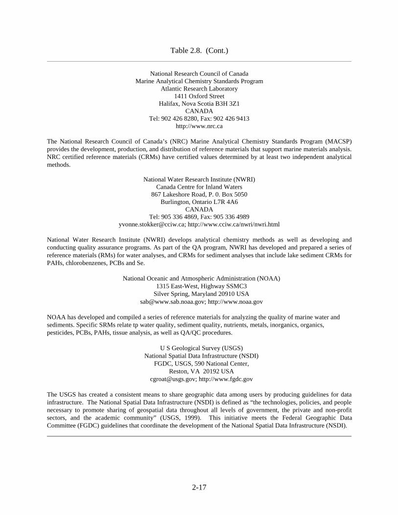
2-17

Table 2.8. (Cont.)

National Research Council of CanadaMarine Analytical Chemistry Standards Program

Atlantic Research Laboratory1411 Oxford Street

Halifax, Nova Scotia B3H 3Z1CANADA

Tel: 902 426 8280, Fax: 902 426 9413http://www.nrc.ca

The National Research Council of Canada’s (NRC) Marine Analytical Chemistry Standards Program (MACSP)provides the development, production, and distribution of reference materials that support marine materials analysis.NRC certified reference materials (CRMs) have certified values determined by at least two independent analyticalmethods.

National Water Research Institute (NWRI)Canada Centre for Inland Waters

867 Lakeshore Road, P. 0. Box 5050Burlington, Ontario L7R 4A6

CANADATel: 905 336 4869, Fax: 905 336 4989

[email protected]; http://www.cciw.ca/nwri/nwri.html

National Water Research Institute (NWRI) develops analytical chemistry methods as well as developing andconducting quality assurance programs. As part of the QA program, NWRI has developed and prepared a series ofreference materials (RMs) for water analyses, and CRMs for sediment analyses that include lake sediment CRMs forPAHs, chlorobenzenes, PCBs and Se.

National Oceanic and Atmospheric Administration (NOAA)1315 East-West, Highway SSMC3

Silver Spring, Maryland 20910 [email protected]; http://www.noaa.gov

NOAA has developed and compiled a series of reference materials for analyzing the quality of marine water andsediments. Specific SRMs relate tp water quality, sediment quality, nutrients, metals, inorganics, organics,pesticides, PCBs, PAHs, tissue analysis, as well as QA/QC procedures.

U S Geological Survey (USGS)National Spatial Data Infrastructure (NSDI)

FGDC, USGS, 590 National Center,Reston, VA 20192 USA

[email protected]; http://www.fgdc.gov

The USGS has created a consistent means to share geographic data among users by producing guidelines for datainfrastructure. The National Spatial Data Infrastructure (NSDI) is defined as “the technologies, policies, and peoplenecessary to promote sharing of geospatial data throughout all levels of government, the private and non-profitsectors, and the academic community” (USGS, 1999). This initiative meets the Federal Geographic DataCommittee (FGDC) guidelines that coordinate the development of the National Spatial Data Infrastructure (NSDI).

2-18

Table 2.9. Website Listing for Methods and Other References

Analytical Chemistry Reference http://www.anachem.umu.se/jumpstation.htmAmerican Public Health Association (APHA) Publications List http://www.apha.org/media/index.htmArctic Monitoring and Assessment Program (AMAP) http://www.grida.no/prog/polar/amap/ASTM http://www.astm.org/British Antarctic Survey http://www.nerc-bas.ac.uk/CREEL Virtual Library http://www.crrel.usace.army.mil/library/crrel_library.htmlEPA 1600 http://www.epa.gov/OST/beaches/entero.htmlEPA CLP Statement of Work http://www.epa.gov/oerrpage/superfund/programs/clp/methods.htmEPA Method 3540c http://www.epa.gov/epaoswer/hazwaste/test/3540c.pdfEPA Method 3611b http://www.epa.gov/epaoswer/hazwaste/test/3611b.pdfEPA Method 5030b http://www.epa.gov/epaoswer/hazwaste/test/5030b.pdfEPA Method 550.1 http://www.horizontechinc.com/Documents/notes.htmEPA Method 8015b http://www.epa.gov/epaoswer/hazwaste/test/8015b.pdfEPA Method 9040b http://www.epa.gov/epaoswer/hazwaste/test/9040b.pdfEPA Method 9041b http://www.epa.gov/epaoswer/hazwaste/test/9041a.pdfEPA Method 9045b http://www.epa.gov/epaoswer/hazwaste/test/9045c.pdfEPA Method 9050b http://www.epa.gov/epaoswer/hazwaste/test/9050a.pdfEPA Method 9060b http://www.epa.gov/epaoswer/hazwaste/test/9060.pdfEPA Methods Index http://www.neis.com/epaindex.htmlEPA Search Engine http://search.epa.gov/EPA SW-846 methods http://www.epa.gov/epaoswer/hazwaste/testGeneral Chemistry Reference http://chemistry.miningco.com/education/chemistry/mbody.htm?terms=chemistry&IASOS Antarctic Information Resources http://www.antcrc.utas.edu.au/iasos/Resources.htmlI-CHEM Environmental Sample Guide http://i-chem.nalgenunc.com/scripts/nalge/i-chem/select/sample.aspIRMM Certification Reports http://www.irmm.jrc.be/rm/cert-reports.htmlItalian Antarctic Research Program http://www.pnra.it/index_inglese.htmlMURST-ISS-A1 http://www.irmm.jrc.be/rm/murst-iss-a1.pdfMURST-ISS-A2 http://www.irmm.jrc.be/rm/murst-iss-a2.pdfNational Environmental Publications Internet Site (NEPIS) http://www.epa.gov/cincl/National Ocean Service Search Engine http://search.nos.noaa.gov/compassNational Oceanic and Atmospheric Administration http://www.noaa.gov/NIST Standard Reference Materials http://ts.nist.gov/ts/htdocs/230/232/232.htmOffice of Ground Water and Drinking Water http://www.epa.gov/OGWDW/Office of Ground Water and Drinking Water Search http://www.epa.gov/watrhome/search.htmlOSHA methods http://www.osha-slc.gov/dts/sltc/methods/index.htmlSRM Index list http://www.epa.gov/owowwtr1/info/PubList/monitoring/html/023.htmlSRM Index list http://www.epa.gov:80/owowwtr1/info/PubList/monitoring/docs/023.pdfStandard Reference Data http://www.nist.gov/srdStandard Reference Materials http://ts.nist.gov/ts/htdocs/230/232/232.htm

3-1

CHAPTER 3.DATA MANAGEMENT

Data management plays a key role in environmental monitoring programs. An effectivedata management system is necessary to meet the environmental monitoring requirements of theAntarctic Treaty System. A properly designed and implemented data management systemprovides effective use of the information collected by environmental monitoring programs andcan fulfill the information requirements of national Antarctic programs.

Data management promotes the efficient and effective use of data collected bymonitoring activities. Data comparability is facilitated through the establishment of datamanagement protocols that disseminate available data to end-users so that local data can beexamined within a regional context. Easily accessible and understandable data also allowsmanagement to identify problems concerning the status and progress of sample/data collectionand analysis. Thus, it provides pertinent information for the appropriate preventative or remedialmeasures that may need to be taken in environmental management. A properly designed datamanagement system promotes long-term preservation of data, which is critical to thedevelopment of baseline information to assess change in the parameters measured. Datamanagement serves as the central node for the flow of data in an environmental monitoringprogram.

The most fundamental objective of data management is to promote efficientdissemination and retrieval of data arising from monitoring and other related activities.

Data management is also necessary to:

(i) ensure the preservation of long-term environmental monitoring data.(ii) facilitate the availability of and access to data.(iii) facilitate comparisons of environmental data with adjacent monitoring programs

providing a broader perspective for data interpretation; and(iv) maximize the utility of data and consequently, the conclusions that arise from their

analysis.

In essence, data management allows information collected in environmental monitoringprograms to be used to make decisions in a timely and cost-effective manner. Early access toinformation encourages preventative rather than reactive actions. Quality control (QC) andquality assurance (QA) are fundamental components of the design and implementation of anenvironmental monitoring program. The high cost associated with activities in Antarctica meansthat questionable data waste valuable and limited resources. Poor quality or misleading data canbe more problematic than an absence of data because it can be misleading and result in thediversion of resources from the real needs to false targets. To ensure proper data dissemination,data management monitors, controls, and facilitates data flow, ensuring data integrity through astep-by-step process in each phase of a program.

A data management plan would typically include: 1) data administration, 2) data control,3) data utilization, and 4) data archiving (Figure 3.1). The integration of these elements into adata management plan is presented below.

3-2

Corrective Actions

PrincipalInvestigatorsReports

ProgramDatabase

Data Archive

DataManagement

Sample/Data Information• Sample• Collection• Chain of Custody Forms• Monthly Status

Sample / DataTracking System

Program Management Status of sample/datacollection and analysis

Dat

a R

eque

sts

Cor

rect

ions

Program Data Transmittal

Metadata

Backup

Data Archive

Data Control

Data UtilizationData Administration

Figure 3.1. The data management plan: 1) data administration, 2) data control, 3) datautilization, and 4) data archiving.

3.1 Data Administration

The first of four elements of a data management system deals with sample and datainformation (Figure 3.2).

Data administration is the element of a data management plan that ensures continuoustracking and custody of samples and data. It includes documentation of data collection andpossession, verification of sample collection completeness, and sample and data security throughchain of custody procedures. Data administration also ensures proper formatting and recordingof data in the database and distribution of data and data products as required among theinvestigators, report authors and agencies.

A detailed summary of the planned sample collections for the entire sampling effortshould be completed prior to the field effort. With this summary a unique sample designation(sample id) for each planned sample collection element can be assigned. These sampledesignations can then be incorporated into a sample tracking system within the program databaseto ensure that the sampling effort is completed in its entirety. Uniformity in the design of sample

3-3

Figure 3.2. Diagram of data administration tasks.

collection forms to be used in the field facilitates subsequent documentation of data. Uniquesample designators are the central component of the sample tracking system. They form thebasis for documenting the collection and labeling of samples in the field. Sample designatorsallow for monitoring of the progress of the sampling and analysis effort in the field, throughanalysis to the distribution of the analytical results. An example of a field sample label thatuniquely identifies the sample is illustrated in Figure 3.3. The label is placed with the sampleand provides collection information in addition to a sample ID. It is best to incorporateinformation into the sample ID beyond simply a sequence number. In the example provided thesample ID incorporates the matrix, year, site, station and sample number.

Project: ANT_00 Site: 5D Station: 37 Date: 01 / 23 / 00

Sample ID: S005D37-7 Gear: SCOOP Matrix: SOIL I.D.: D. ALSUP

Comments: 2 cm ice/snow overlay

Figure 3.3. Field sample collection label example.

Forms developed prior to the field effort are an integral part of the samplecollection/tracking component’s success. Appropriate forms allow accurate and completedocumentation of the sample collection process. The uniformity gained by preparation ofstandardized forms facilitates documentation and ensures the completeness and accuracy of dataentered into the program database. An example of a sample collection form to be used in thefield is shown in Figure 3.4.

Corrective Actions

ProgramDatabase

Data Administration

Sampling planField forms design

Samplecollection

Copies of completedfield collection forms

andChain of Custody forms

DataManagement

Preliminary QCscreen


StatusReports

ResearchersManagersAgencies

3-4

Figure 3.4. Sample collection field form example.

Careful attention to designing data collection forms promotes accurate, efficient datacollection and a smooth transition from the field into the project database. In addition,thoughtful form design prevents neglecting items whose omission may compromise qualitycontrol, prevent complete statistical analyses or degrade the accuracy of any conclusions.

Collection forms are designed to ensure that all essential information is recorded in thefield. In addition, the forms are designed to ensure that:

1) data are collected in the most efficient order;2) all pertinent experimental information (sample type, location, sampling date,

sampling time, etc.) is included;3) areas on the form where observations are recorded are clearly labeled and adequate

space is available to accommodate the maximum expected value, assuring simplicityand legibility of the data; and

4) additional space for recording pertinent comments is available to assure correctinterpretation of the observations.

3-5

Immediately after each field effort is completed, copies of the field collection forms areforwarded to Data Management. These forms can be scanned electronically and placed into theprogram database for permanent documentation archival. Information contained in the copies ofthe field collection forms is entered into a sample/data tracking system and the status of thesamples collected during the particular field effort is updated. Reports can then be produced thatdescribe and define the sample collection information. The reports are distributed to the researchteam, providing an overview of data collection and a reference to sample and locationnomenclature.

Continuous tracking of samples and data is accomplished using a sample/data trackingmodule in conjunction with tracking protocols. Custody of samples and data is documented bychain-of-custody forms and data transmittal forms for each change of possession. These formsprovide the necessary security as one custodian relinquishes the samples to the next custodianwith signatures. Dates and times of transfer are noted on the forms. An example of a chain ofcustody form is shown in Figure 3.5.

Figure 3.5. Example of Chain of Custody Form.

Before a data file is incorporated as valid data into the program database, it is subjectedto a data screening analysis--a quality control procedure designed to minimize errors. Samplecollection data sheets or laboratory reports are compared to data file listings reviewing the latterfor accuracy and completeness (Figure 3.6). This screening includes range checking andthematic scanning of data to detect potential outliers, calculation of a statistical summary, whichincludes minimum, maximum, and mean values, numbers of valid observations, and totalnumber of observations in the data file. This information and tabular listings of the data file aresent to the appropriate investigator for review. The investigator reviews the printouts and

3-6

statistics for errors. Any errors in the data file are corrected, and new printouts are generated andsent to the investigator. After the investigator certifies that the data file is valid, the data file isincorporated into the program database.

Figure 3.6. Example of Sample Status Form.

Copies of all chain-of-custody forms (Figure 3.5) and data transfers are sent to datamanagement. This information can be used to update the status of the samples. It primarilyconsists of files of milestones for each sample. Status milestones are generally as follows:

1) sample collection in the field,2) sample transmittal and receipt by the laboratory,3) processing status within the laboratory and completion of the analysis,4) transmission of the analytical results to data management,5) data entry,6) data validation,7) incorporation of validated data into the program database,8) transmittal of the sample/data to the final repository, and9) archival.

3.2 Data Control

The purpose of data control is to monitor progress of the data flow, identifying gaps inthe information supplied and to signal further processing requirements. Data control proceduresenable the documentation of data availability, data reduction, and data analysis to be determinedwhenever necessary (Figure 3.7).

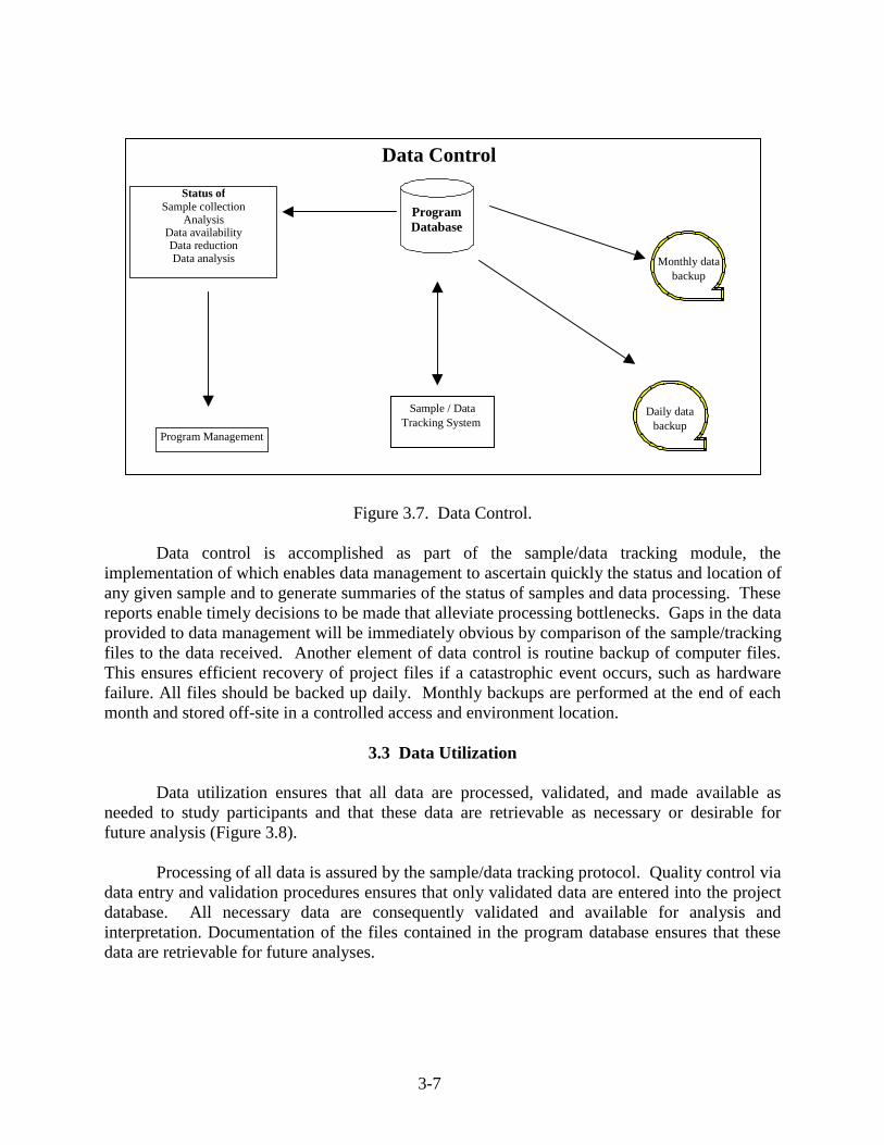
3-7

Figure 3.7. Data Control.

Data control is accomplished as part of the sample/data tracking module, theimplementation of which enables data management to ascertain quickly the status and location ofany given sample and to generate summaries of the status of samples and data processing. Thesereports enable timely decisions to be made that alleviate processing bottlenecks. Gaps in the dataprovided to data management will be immediately obvious by comparison of the sample/trackingfiles to the data received. Another element of data control is routine backup of computer files.This ensures efficient recovery of project files if a catastrophic event occurs, such as hardwarefailure. All files should be backed up daily. Monthly backups are performed at the end of eachmonth and stored off-site in a controlled access and environment location.

3.3 Data Utilization

Data utilization ensures that all data are processed, validated, and made available asneeded to study participants and that these data are retrievable as necessary or desirable forfuture analysis (Figure 3.8).

Processing of all data is assured by the sample/data tracking protocol. Quality control viadata entry and validation procedures ensures that only validated data are entered into the projectdatabase. All necessary data are consequently validated and available for analysis andinterpretation. Documentation of the files contained in the program database ensures that thesedata are retrievable for future analyses.

Program Management

Status ofSample collection

AnalysisData availabilityData reductionData analysis

Data Control

ProgramDatabase


Daily databackup

Monthly databackup

3-8

Figure 3.8. Data Utilization.

3.4 Data Archive

Data archival is a method for the safe storage and easy retrieval of all accumulated data,photographs and videotapes (Figure 3.9). Data archives should be maintained on high capacity,removable media. One backup should remain in data management’s possession. Files will beroutinely archived to this tape. The other backup should be maintained in a separate location.Archived files that are accumulated on the first archive tape will be periodically copied to theoff-site tape. This procedure assures the permanency of the data archives.

Figure 3.9. Data Archive.

Photographs can be scanned to provide a digital copy and archived on CD to provide forsafe storage of the image. All original photographs and negatives are maintained in a separate,environmentally controlled storage area. Program videotapes should be copied and stored in asimilar fashion.

Program Data DistributionMetadata

Data Archive

DataArchive

ProgramDatabase

PhotosNegatives

VideoResearch logs

Field notesRaw data

Compiled dataScans

Data ArchiveStorage

DataManagement

Dat

a R

eque

sts

Cor

rect

ions

Data Utilization

ProgramDatabase


ResearchersManagement

Agencies

3-9

All data collected during the course of a project should be accompanied by metadata thatcompletely describes the physical and logical sizes and formats of all files in the data set. Also,it should provide sufficient information and references to completely identify all of the data inthe data sets.

All data should be associated with “metadata” or data about the data, i.e., informationdescribing the data in question. Amongst other information, this will provide details of theinvestigators or data source, collection, content, range and resolution of the data and qualityassurance information. This metadata should be intimately linked to the data so that it isimpossible to access a dataset without also receiving information about that dataset. Thus data ofdifferent origins (e.g., data collected as part of scientific research or as part of a monitoringprogram) and quality will be easily identifiable. A metadata file should be associated with alldata and should conform to the guidelines as established by the National Data Centers as part ofthe Antarctic Data Directory.

3.5 Geographic Information Systems

A geographic information system (GIS) is a computer-based tool for viewing, mappingand analyzing phenomena that are spatially situated (Clarke 1997). GIS technology integratescommon database operations with functions and tools, such as data storage, analysis, and displayof geographic information as well as spatial data integration with other data resources. Geo-referenced data contain an explicit geographic reference, such as a latitude and longitude ornational grid coordinate, or an implicit reference such as objects tacitly related to each other inspace (i.e., distance) so that thematic data layers can be linked geographically (Figure 3.10).Geographic information systems view two fundamentally different types of geographic data-vector and raster. Vector data is encoded and stored as a collection x,y coordinates that formpoints, lines, and polygons. The location of a point feature, such as a sampling point, can bedescribed by a single x,y coordinate. Linear features, such as roads and rivers, can be stored as acollection of point coordinates. Polygonal features, such as buildings or river catchments, can bestored as a closed loop of coordinates with an area and perimeter. Vector data are useful fordescribing discrete features, but less useful for describing continuously varying features such assoil type. Raster data models continuous features as an image comprised of a collection of gridcells, for example a scanned map or picture. Both vector and raster data are useful for storinggeographic data and both have unique advantages and disadvantages. Once digitized, data typesrequired for a particular GIS project will have to be transformed to the coordinates and scalenecessary to view and analyze phenomena of interest on a landscape. Elements of geographicinformation are discernable at a variety of scales as reported by Kennicutt and Wolff (1998), andbefore this information can be integrated, it must be transformed to the appropriate scale foranalysis (dependent upon the degree of detail or accuracy required).

3-10

Figure 3.10. An example GIS composed of data layers of spatial information registered to acommon map projection.

4-1

CHAPTER 4.SAMPLE COLLECTION, HANDLING, AND PRESERVATION

Proper sample collection, handling, and preservation is critical to any monitoring program.The quality of data produced is dependent on collecting a representative sample whose contents arepreserved intact until the time of analysis.

Sampling in support of Antarctic monitoring programs presents special challenges in thatthe weather is often severe and sample collection may require the sampling of or through afrozen medium. While it is beyond the scope of this manual, a brief discussion of the types oftechniques available for “through the ice” sampling is provided. Special circumstancesencountered include collection of samples under the ice, keeping sampling access holes open,freezing or preserving of samples upon retrieval, and performing these difficult operations in aclean non-contaminating manner.

It is also recognized that many Antarctic programs will not be equipped to carry out theanalysis of samples themselves. The samples may be exported from the continent for analysis incommercial laboratories. In addition, all sampling locations will not be in close proximity tolaboratory facilities that can perform the analyses on site. This requirement to transport samplesfrom the site and possibly to laboratories within the home country presents special challenges forthe handling and preservation of samples in a manner that maintains the integrity of the samples.Such things as sample size, sample type, and the chemicals used as fixatives may all be concernsfor transported samples. While it is not possible to address all of the issues that might beencountered, this chapter provides general guidance on the procedures that will aid in copingwith these unique characteristics of monitoring in Antarctica. Within each method, a briefsummary is provided of any issues that one should be aware of when considering the sampling,handling and preserving of samples in Antarctica.

Fundamental to all sampling techniques is prevention of the introduction of foreignmaterials that will interfere with the intended analysis. In many cases this requirement is easilymet by cleaning the sampling gear and receiving containers by standard methods. It is alsoimportant that foreign materials from the surrounding atmosphere be prevented from beingintroduced to the sample during collection activities. Often the sampling person will need towear appropriate gloves or other coverings to prevent contamination by the collector. Therequirement for “clean” conditions becomes more and more demanding as the concentration ofthe analytes of interest gets lower and lower. The addition of small amounts of interferants willconsequently cause large mis-estimations in analyte concentrations. The types of interferants aredependent on the parameter being measured and thus cleaning techniques are discussed on amethod-by-method basis. For example, plastic bottles cleaned by acid are appropriate for watersamples collected for trace metal analysis but glass bottles cleaned with detergent, distilledwater, and solvents are preferred for organic contaminants such as hydrocarbons. Variouspreservation techniques can be employed from freezing to chemical fixatives depending on theparameter of interest and the delay between collection and analysis. These preservation methodsmust retain the sample’s original attribute of interest at the time of collection and also must notintroduce interferants into the sample.

4-2

In some instances, “traveling” and “field blanks” are incoporated as part of the analyticalprotocol. In these instances, sample containers accompany the equipment into the field and aresubjected to all of the events during sampling other than those of the actual sampling. Reagents areadded and the “blank” is returned to the laboratory for analysis. Should contamination occur, “fieldblanks” are useful in identifying the portion of the procedure that leads to contamination and thussuggests a remedy for any future sampling. There also needs to be procedures in place to dispose ofany hazardous materials (i.e., solvent rinses) generated in the field.

4.1 Wastewater

Sampling program objectives dictate the location and frequency of wastewater sampling.For example, to determine if water quality objectives are being met for a sewage treatment plant,sample locations are typically chosen at the inflow to the treatment facility, the effluent from thetreatment facility, and the water supply. Representative sampling is an important considerationfor properly characterizing wastewater streams. Chemical and biological levels in wastewatershould be considered dynamic variable since wastewater flow rate and wastewater qualitycontinuously change. Obtaining samples that represent the wastewater flow over time periods ofdays, months and years is difficult at best. Diurnal fluctuations occur in concentration and flowvolume; seasonal fluctuations occur in concentration, flow volume, and temperature; and labrelated contributions to the system might cause wastewater characteristics to change on a short-or long- term basis. Given the variable nature of wastewater, it is advisable that samples becollected that represent “average” characteristics and approximate characteristics under moreextreme conditions. The wastewater quality would be expected to vary inversely with thenumber of individuals present on a station at any given time. Wastewater treatment facilitiesvary from discharging raw sewage to processing the sewage on-site prior to discharge dependingon the station and the host country.

Wastewater samples can be collected manually or by using automated samplers. Caremust be taken to avoid the introduction of extraneous materials when using either method ofwastewater sampling. There is minimal initial cost for manual sampling; however, automatedsamplers are particularly well suited to higher sampling frequencies. Some advantages anddisadvantages of manual and automated sampling are tabulated in Table 4.1 (from EPAHandbook for Sampling and Sample Preservation of Water and Wastewater, 1982). Anautomated sampler will have a sample gathering subsystem (mechanical, forced flow, or suctionlift systems), a sample transport system (typically flexible plastic tubing), and a sample storagesystem (typically a two gallon container for a composite sampler). Wastewater samplers arecommercially available that collect a time weighted composite sample. A grab sampler is anexample of a manual sampling method that typically consists of a telescoping pole thataccommodates various sized sample collection bottles at the distal end. Grab samples can alsobe collected from the wastewater stream using a pump, scoop, vacuum, or other suitable device.Grab samples are individual discrete samples collected over a period of time not to exceed 15minutes. These samples will characterize the water quality at one particular time. Collection ofa composite sample consisting of a number of discrete grab samples is necessary for determiningaverage wastewater concentrations and for calculating mass per unit time loading. Each discretesample should be at least 500 mL and each composite sample should be a minimum of 7.57 L.This will provide data that is considered representative of average wastewater characteristicsthroughout the day while minimizing sample holding times. A careful review of flow

4-3

Table 4.1. The Advantages and Disadvantages of Manual and Automatic Sampling ofWastewaters (EPA 1982).

Type Advantages Disadvantages

Manual 1) Low capital cost. A) Probability of increasedvariability due to samplehandling.

2) Compensates for varioussituations.

Inconsistency in collection.

B) High cost of labor, assumingseveral samples taken on adaily basis.

3) No maintenance. Repetitious and monotonoustask for personnel.

4) Can collect extra samples ina short time when necessary.

Automatic 1) Consistent samples. A) Considerable maintenancefor batteries & cleaning.

2) Probability of decreasedvariability caused by samplehandling.

Susceptible to plugging bysolids.

3) Minimal labor requirementfor sampling.

B) Restricted in size to thegeneral specifications.

4) Has capability to collectmultiple bottle samples forvisual estimate of variability& analysis of individualbottles.

Sample contaminationpotential

monitoring records and reports generated by a treatment facility will also be helpful in assessingthe seasonal characteristics of the wastewater throughout the year and in determining samplingfrequency.

Once a sample is taken, the sample should be maintained in the same condition as when itwas collected. When it is not possible to immediately analyze collected samples, samples shouldbe properly preserved (Table 4.2). Biological activity such as microbial respiration, chemicalactivity such as precipitation or pH change, and physical activity such as aeration or hightemperature should be kept to a minimum. Methods of preservation include cooling, pH control,and chemical addition. Freezing is usually not recommended. The length of time that aconstituent in wastewater will remain stable is related to the character of the constituent and thepreservation method used. The EPA Handbook for Sampling and Sample Preservation of Waterand Wastewater (EPA 1982) provides detailed guidelines on sampling, preservation techniques,and analysis of wastewater samples.

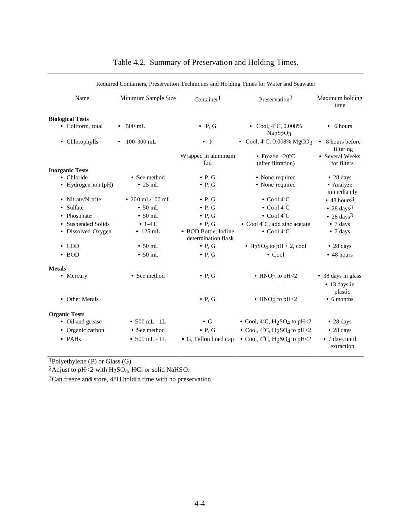
4-4

Table 4.2. Summary of Preservation and Holding Times.

Required Containers, Preservation Techniques and Holding Times for Water and Seawater

Name Minimum Sample Size Container1 Preservation2 Maximum holdingtime

Biological Tests• Coliform, total • 500 mL • P, G • Cool, 4oC, 0.008%

Na2S2O3• 6 hours

• Chlorophylls • 100-300 mL • P • Cool, 4oC, 0.008% MgCO3 • 8 hours beforefiltering

Wrapped in aluminumfoil

• Frozen –20oC(after filtration)

• Several Weeksfor filters

Inorganic Tests• Chloride • See method • P, G • None required • 28 days• Hydrogen ion (pH) • 25 mL • P, G • None required • Analyze

immediately• Nitrate/Nitrite • 200 mL/100 mL • P, G • Cool 4oC • 48 hours3

• Sulfate • 50 mL • P, G • Cool 4oC • 28 days3

• Phosphate • 50 mL • P, G • Cool 4oC • 28 days3

• Suspended Solids • 1-4 L • P, G • Cool 4oC, add zinc acetate • 7 days• Dissolved Oxygen • 125 mL • BOD Bottle, Iodine

determination flask• Cool 4oC • 7 days

• COD • 50 mL • P, G • H2SO4 to pH < 2, cool • 28 days

• BOD • 50 mL • P, G • Cool • 48 hours

Metals• Mercury • See method • P, G • HNO3 to pH<2 • 38 days in glass

• 13 days inplastic

• Other Metals • P, G • HNO3 to pH<2 • 6 months

Organic Tests• Oil and grease • 500 mL - 1L • G • Cool, 4oC, H2SO4 to pH<2 • 28 days

• Organic carbon • See method • P, G • Cool, 4oC, H2SO4 to pH<2 • 28 days

• PAHs • 500 mL - 1L • G, Teflon lined cap • Cool, 4oC, H2SO4 to pH<2 • 7 days untilextraction

1Polyethylene (P) or Glass (G)2Adjust to pH<2 with H2SO4, HCl or solid NaHSO43Can freeze and store, 48H holdin time with no preservation

4-5

Table 4.2. (Cont.)

Required Containers, Preservation Techniques, and Holding times for Snow

Name MinimumSample Size

Container1 Preservation2 Maximumholding

time

Inorganic Tests• Particulates • See method • P, G • Cool 4oC,

add zinc acetate• 7 days

Metals• Mercury • 150 mL

(melted)• P, G • HNO3 to pH<2 • 38 days in

glass• 13 days

in plastic• Other Metals • 350 mL

(melted)• P, G • HNO3 to pH<2 • 6 months

Organic Tests• Oil and grease • 500 mL-1L

(melted snow)• G,

Teflon lined cap• Cool, 4oC, H2SO4 to pH<2 • 28 days

• PAHs • 500 mL-1L(melted snow)

• G,Teflon lined cap

• Cool, 4oC, H2SO4 to pH<2 • 7 daysuntil

extraction• TPH • 500 mL-1L

(melted snow)• G,

Teflon lined cap• Cool, 4oC, H2SO4 to pH<2 • 7 days

untilextraction

Required Containers, Preservation Techniques, and Holding Times for Soil/Sediment

Name MinimumSampling Size

Container1 Preservation2 Maximumholding

time

Miscellaneous Tests• Grain Size • 30 g • P, G • Cool 4oC • Indefinite• Organic carbon • 5 g wet weight • P, G • Frozen –20oC • Indefinite

Metals• Mercury • 1g wet weight • P, G • Frozen –20oC • 1 year• Other Metals • 1g wet weight • P, G • Frozen –20oC • 1 year

Organic Tests• Oil and grease • See method • G,

Teflon lined cap• Frozen –20oC • 1 year

• Organic carbon • See method • G,Teflon lined cap

• Frozen –20oC • 1 year

• PAHs • See method • G,Teflon lined cap

• Frozen –20oC • 1 year

1Polyethylene (P) or Glass (G)2Adjust to pH<2 with H2SO4, HCl or solid NaHSO4

4-6

4.2 Marine and Freshwater

Marine and freshwaters are often sampled for a range of properties in support ofmonitoring activities. In many cases the body of water is substantial enough and the parametersof interest are heterogeneously distributed throughout the water body so that multiple samplesare required. Samples can be collected areally to cover the horizontal dimensions of the waterbody and/or vertically to detect gradients within the water column. These spatial collections areoften needed since pollutants enter a water body at a point source and then are diluted by mixingwith uncontaminated water. The areal extent of the introduced materials is often key indetermining the seriousness of the contamination and what secondary effects may result. Forexample, introduction of sewage via an outfall in a high energy environment (extensive waveand wind action) may cause little perturbation of the surrounding marine environment becausethe toxicants or bacteria are rapidly diluted and/or are transported from the area by currents. In aclosed bay where the water resides for long periods of time, the toxicants would tend toaccumulate and increase to levels that may impact the resident biota. In the case of sewage, theintroduction of organic carbon (measured by BOD and COD) could cause the resident bacteriato completely consume the oxygen in the water column producing eutrophication. The physicalproperties and dynamics of water bodies in general tend to result in a heterogeneous distributionof contaminants, thus there is a need for spatial sampling designs.

Water properties can be sampled using bottles to collect discrete samples or through the useof in situ sensors or both. Sampling equipment can be deployed by a variety of means. Keyconsiderations in selecting sampling method are that samples are collected in a manner that ensuresthe safety of the sampling personnel and the integrity of the samples. This section discusses the useof water bottles to collect water samples and in situ instrumentation.

4.2.1 Discrete Water Sample Collection

Water-bottle samplers are relatively simple devices that generally consist of some type ofcylindrical tube with stoppers at each end and a closing device that is activated by a messenger or anelectrical signal. Sample bottles can also be manually filled and stoppered for snow and/or runoffsampling by directly submerging the bottle in the water to be sampled. The most commonly usedsamplers are the Van Dorn, Niskin, Nansen, and Go-Flo samplers. Each device samples a discreteparcel of water at a designated depth. Each sampler can be attached directly to a wire or cable andlowered to the desired sampling depth. Frequently in marine settings, multiple water samplers arefixed on a rosette frame so that several depths can be sampled during one cast or replicate samplescan be taken at the same depth using electronic releases.

Prior to deployment, the stoppers of water-bottle samplers are cocked open. It is critical thatthe interior of the sampler and stoppers remain free from contamination. Personnel should avoidtouching the insides of the sampler and/or stoppers. The interior of each water bottle samplershould be washed periodically with 10-percent hydrochloric acid (non-metallic bottles only). Thisshould be repeated if contamination is suspected. As an alternative to the acid washing, alaboratory cleaning solution can be used. The gear should then be well rinsed with ambient water.

After cocking, the sampler is lowered to a designated depth or deployed manually by hand.The sampler is open at both ends so that water is not trapped within the device as it is being loweredinto the water. Lowering the sampling bottle through any obvious surface film should be avoided if

4-7

at all possible. Once the sampler reaches the desired depth, it is allowed to equilibrate with ambientconditions for 2-3 minutes before being closed. Equilibration time is extended to five (5) minutes ifthermometers are attached for the measurement of temperature.

After equilibration, the closing device can be activated by messenger or electrical signal ormanually, and the sampler is retrieved. In some cases (e.g., for deep water), two samplers can beused simultaneously for each depth. A second sampler provides a backup to the primary sampler incase the latter device misfires or will not trigger or additional sample is required by the analyticalmethod. To ensure that all subsamples at a particular depth are collected from the same waterparcel, it is recommended that they all be taken as a single cast.

Once the water sampler is returned, the stoppers should be checked for complete seals. If astopper is not properly sealed, water from the sampled depth may have been replaced by water fromanother depth. The water sample should be retaken if it appears the water sample has beencompromised.

Acceptable water samples are subsampled as soon as possible (i.e., within 15 minutes)because appreciable delay may result in non-representative subsamples. For example, measurementof variables sensitive to biological alteration (e.g., dissolved oxygen, turbidity, color, nutrients) orsettlement within the water sampler (e.g., total suspended solids, phytoplankton) can be biased bysubsampling delays. Samples for dissolved oxygen measurements should be the first samplescollected. If samples for other variables are not collected within 15 minutes after sample collection,the sampling bottles should be shaken prior to subsampling to ensure a homogenous water sample.

One challenge to water sampling in Antarctica is that the water bodies of interest areoften covered with a substantial layer of ice. Various techniques are available for penetrating iceincluding chipping and/or some type of auger or drilling device. The challenge is to use thesetechniques in a non-contaminating and safe manner. Often the size of the water sampler willrequire a large access hole for through-the-ice sampling.

4.2.2 In Situ Sensors

A wide variety of instruments capable of measuring water column variables in situ areavailable. Most are deployed on a wire, conducting cable, or by manual placement in the water ofinterest. The sensors measure the variables of interest and transmit data in the form of electricalsignals to external or internal recorders or meters. The simplest instruments measure conductivity(i.e., for conversion to salinity), temperature, and water pressure (i.e., for conversion to depth).Additional sensors and instrumentation can be included to measure a variety of additional variablessuch as dissolved oxygen, pH, transmissivity (i.e., an index of turbidity), and oxidation-reductionpotential. Water transparency can be measured using an irradiance meter. Chlorophyll a can bemeasured in situ using a fluorometer. Generally, the operating manuals supplied with theseinstruments provide detailed descriptions of how to calibrate, operate, and maintain the equipment.If a particular manual lacks sufficient detail, the manufacturer should be contacted for specificguidance. An annual or semiannual intercalibration is useful for ensuring the comparability andquality of measurements.

The major advantages of in situ instrumentation is the ability to measure continuous depthprofiles of water-column variables and the measurements are made on-site requiring no sample

4-8

return. Continuous profiling eliminates the need to select discrete sampling depths. In addition,continuous profiling can identify water-column discontinuities and plumes that may not be detectedif measurements are restricted to discrete depths. In situ sensors also limit the need for preservationand transport of samples from the field to the laboratory. However, some sensors require substantialsupport facilities or equipment to maintain electronics.

4.2.3 Ice and Through-Ice Sampling

The specific program objectives will determine the sampling methods used. Theseobjectives can range from analyzing ice cores for changes in analytes as a function of depth(time) to ice serving as an impediment to collection of water samples from below the ice.

Ice cores drilled through an ice sheet provide a sample of all the layers of snow that haveaccumulated over time. Ice cores can provide uniquely detailed samples on time-scales rangingfrom decades to several hundred thousand years. Ice cores are collected using a wide spectrumof ice drills ranging from hand augers, mechanical drills, to extensive electro-mechanical drillsthat are capable of retrieving cores with a 13.5 cm diameter from depths as great as 5000 meters.Ice drilling is enhanced by the use of a drilling fluid (e.g., hot water, ethanol, a mixture ofaviation fuel and freon) some of which are considered contaminants. A summary of differenttypes of ice drilling equipment typically used is provided in Table 4.3.

Following recovery of an ice core, the core must remain in a frozen state until the ice issampled, typically in a laboratory off the ice. Once at the facility, sampling an uncontaminatedportion of the core becomes important. The outside of the core has been in contact with thedrilling equipment and may not be representative of the ice sheet. A number of techniques havebeen developed where the interior of the ice core is melted (without also melting the outer layerof the core) and the water is then collected and analyzed. These techniques are outside the scopeof this manual and are available from the Greenland Ice Sheet Project (GISP), AntarcticAstronomy and Astrophysics Research Institute, International Glaciological Society (IGS),European Project for Ice Coring in Antarctica (EPICA), and the Polar Ice Coring Office of theNational Institute of Polar Research (PICO).

Through-ice sampling provides a method for collecting water samples from below icesheets. Sites should be chosen where the water is known to be deep enough to avoid stirring upbottom sediments when penetrating the ice. Depending on the thickness of the ice, a hand ormotorized auger can be used. Extremely thick ice may require a more elaborate drilling system.Once the hole is open, traditional water and sediment sampling equipment can be lowered intothe underlying water and samples collected. An extensive survey of a lake may require morepenetrations than is desirable or feasible. In these instances, the use of divers to collect thesediment, water, and biological samples is an alternative.

4.3 Snow

Depending on the analytes of interest, various types of sample containers have beenrecommended for the collection of snow and ice samples. The common feature amongcontainers for the collection of snow is that they need to be meticulously cleaned. Container lidsneed to have a water-proof seal for transport of the melted snow. The choice of samplecontainers for inorganic analytes, including trace metals and ions, are polyethylene orpolypropylene (e.g., Nalgene) bottles that are first rinsed with distilled water and then soaked indistilled water for at least 24 hours. After soaking, the bottles are again rinsed with fresh

4-9

Table 4.3. Drill Types.

Drill Title Type DepthCapability

Core Diameter

Jiffy Auger InternalCombustion

1 to 5 m None

Lightweight Auger: 20 msystem

Manual 20 m/50 m 7.6 cm/10.2cm

82 mm Eclipse Drill Electro-Mechanical

240 m 82 mm

4 inch Drill Electro-Mechanical

353m**500 m*

10 cm

5.2 inch Wet/Dry Drill Electro-Mechanical

200 m - 5,000m

13.5 cm

5.2 inch Rock DrillAttachment

Diamond Coring 50 m 1.3 inch

30 cm Dry Drill Electro-Mechanical

200 m** 30 cm

Thermal Drill Electro-Thermal 312 m4,000 m**

8.7 cm

Hot Water Shot Hole Drill Hot Water 30 m 4.0 inch holeAMANDA Drill Deep Hot Water 220 m

2200 m30.0 inch hole

* Depth capability is dependent on ice temperature and strain history; usual limit is corequality or hole closure.

** Untested to specified depth.

distilled water. The samples are then dried in a clean environment and sealed until sampling. Ifhydrocarbons are the target analyte, glass bottles are preferred that have been washed with lowresidue detergent, rinsed with distilled water, rinsed with solvents (acetone to dry and methylenechloride to remove any film), and dried in a clean environment. Often the glass bottles arecombusted at 450ºC if the closures will not be distorted by heat. The bottles are sealed withprecombusted aluminum foil and stored until sampling. Sampling utensils also need to bemeticulously cleaned by similar procedures.

The following procedures are extensive and in most instances a surficial snow samplewill be adequate for detecting atmospheric deposition. However, snow and ice profiles canprovide a retrospective look at contamination in the area. This method should be adapted to theneeds of the individual monitoring program.

4.3.1 Sampling Procedures

Snow is often manually collected by using scrapers made of polycarbonate (Lexan) orplexiglass. Three different sizes are recommended (15 x 15 cm, 10 x 10 cm, and 10 x 2 cm) tomake the sampling more efficient. Beveled edges on several sides facilitate the collection ofsnow by scraping. A non-beveled handle makes the scrapers easier to handle. Scrapers arecleaned using methanol and a small brush for scrubbing. The scraper should be rinsed withpurified water and allowed to soak for 48 hours in purified water. After soaking the scrapers arerinsed three times and placed in a new bath of purified water for 24 more hours of soaking. The

4-10

scrapers are then rinsed and dried in a clean environment and stored in sealed containers baggedin polyethylene bags. It is recommended that the field technician wear polyethylene glovesduring the sampling. Scrapers should be carefully rinsed and cleaned between samplings. Incases were very low levels are expected, clean suits (polyester or tyvek) and particle masks maybe required to prevent contamination of the snow samples.

In addition, it is useful to also have a plastic shovel to initially clean the sampling wall, ametal shovel for snowpit excavation, a tape measure to accurately record the depth of thesampling, and a snow density kit to measure snow accumulation rates.

4.3.2 Snowpits

In locations that are primarily snow covered, it is recommended that sampling be done byexcavating snowpits to ensure undisturbed samples are retrieved.

After a snowpit site has been selected, all sampling equipment should be at the site toallow for immediate sampling of the snowpit upon completion of the excavation. First, thedirection of the wind is determined and a clean, dedicated metal shovel is used to define an edgeperpendicular to the wind direction about 1.5 to 2 meters long. This will be the sampling wall.Nothing should be placed upwind of the site. Also during digging, nothing (e.g., hands, body,etc.) must touch the wall to be sampled, other than the shovel. The upper 10-50 cm willprobably be most easily removed using the shovel. The top of the snowpit should measure ~2 x1.5 meters to give sufficient room for working in the pit. Once loose snow is removed from theupper 10-50 cm, a snow saw can be used to cut blocks and using the pointed or square shovelbreak the blocks free. All spoils (excavated snow) from the pit must be placed downwind fromthe sampling wall. If there is blowing snow, then a snow wall may be built on the upwind side ofthe pit. This should be done using blocks cut out of the pit. If a wall is built, it should remain 1meter from the sampling wall. Once the wall is built no one should be upwind of the pit. Finaldepth of the snowpit should be ~2.1 meters (for a 2 meter snowpit). To help facilitate thesampling of the pit a large, firm block can be left in the bottom of the pit to stand on whilesampling the top of the pit.

4.3.3 Snowpit Sampling

Two people are recommended for sampling the snowpit: one person who samples the pitand the other person assists with bottles and note taking. Upon snowpit excavation andcompletion, it is recommended that the sampler wears a clean suit, particle mask, andpolygloves. The other person should be dressed in clean non-particulating clothing as well as aparticle mask and clean dedicated gloves. Using the clean shovel, a ~50 cm wide section of thesampling wall is removed and at least 15 cm into the wall from top to bottom of the samplingwall. Once this is done, the spoils should be removed from the pit and the plastic shovel shouldbe placed in a clean plastic bag for use in the next snowpit.

The sampler should replace the used polygloves. Next, one of the 15 x 15 cm scrapers isused to remove ~5 more centimeters from the cleaned shovel surface. This scraper can then beinserted into the corner of the cleaned sampling wall and act as a shelf to place the sample cuplid while sampling. Next, one of the 10 x 10 cm scrapers is used to clean the sampling surfaceback several centimeters down (about 50 cm from the top of the pit). This step is repeated as

4-11

samples are collected down the wall. The 10 x 10 cm scraper can be inserted into a cleanedsection of the wall to keep clean for the next 50 cm of sampling. A measuring tape can be hungdown the wall to accurately determine depth of sampling. A scraper at the surface will helpalleviate the tape cutting into the surface.

The correct sampling template corresponding to the desired sample interval (ideal sampleinterval is 8-10 samples/year) is selected. By keeping the index marker parallel to the surface,the wall is marked using the template. Several passes may be necessary to get good markings onthe snow wall. The template is placed into a cleaned section of the wall. The wall is now readyfor sampling. The helper should then hand the sampler a sample cup with the lid pre-loosened.The sample cup lid is removed and placed on the “shelf” made by the 15 x 15 scraper with theinside of the lid down. One of the 20 x 2 cm scrapers is used to remove ~1 cm just above theline made by the template. Then the sample cup is placed lightly against the wall and filled withsnow using the scraper. The scraper is placed into a clean section of the wall and the lid is putback on the cup. Cups are exchanged with the helper and collection is contined until one isabout 3-4 samples from the marks from the template. Using the previous marks as a guide,additional marks are made down the cleaned snow wall. The 10 x 10 scraper is used to pre-cleanthe wall once the ~50 cm cleaning is reached. Using the measuring tape, true depth can be cross-correlated with sample depth. As the sampling depth in the snowpit is increased, the snowhardness will increase. It may be necessary to use the 20 x 2 cm scraper like a chisel in order tobreak up the snow.

Sample cups must be checked each time to assure they are in order. The helper shouldpre-loosen the lids to the sample cups before handing it to the sampler. Once the sample iscollected and cup returned to helper, it is necessary to tighten the lid as much as possible.Samples must be placed out of the direct sun to prevent melting. The helper records notes aboutthe snowpit which include description of the snow from the sampler, container numbers, generalweather and sampling conditions and miscellaneous notes related to sampling (e.g., stratigraphy,grain size, etc.).

Other guidance includes:

• while sampling, check polygloves often for rips or tears and replace as necessary;• remember, 2 pairs of polygloves work better than one pair;• record good notes on snowpit excavation and measurement;• always have an additional “clean” section on the pit wall (this section can be used to

clean tools that may drop to the pit floor, the snow is a clean, abrasive cleaner); and• remember to keep hands away from the particle mask (if it touches the polygloved

hands, the polyglove should be replaced; the mask concentrates breath which hasvery high concentrations of ions measured in the snowpack).

4.3.4 Stratigraphy and Physical Studies

Density and physical stratigraphy can be recorded after the sampling of the snowpit.Parameters such as layer thickness, hardness, color, crystal size and shape, location and thicknessof ice or debris bands should be recorded. Photographs of the pit wall should be taken to recordthe visible structure and layering.

4-12

4.3.5 Snow Pack Depth

Snow pack depth gives the sampler an idea of the snow’s physical properties. Becausemany factors can play a role in snow redistribution, such as: annual temperature, wind, energy ormoisture transfer, and physiography, a snow depth measure gives the sampler an idea of howthese factors effect snow pack depth and distribution.

To measure snow pack depth:

• Take 2 sections of aluminum poles approximately 1/4 inch in diameter. The firstsection should be 6 meters in length and the second section should be 3 meters inlength. The sampler or “snow probe” should have the aluminum poles processed sothat the 3 m subsection can be fitted onto the 6 m section. These poles should havehatch markings every centimeter so that the sampler can measure snow depth.

• While on the snow pack, place the pole into the snow pack in a straight perpendicularfashion until a hard surface hampers pole movement into the pack.

• Finally, note the final measurement, or the cm hatchmark at the snow line.• Repeat this process at nine (9) other randomized points in the snow pack.

4.4 Sediments and Soils

The most common sampling device for marine surficial sediments is some type of bottomgrab sampler. However, various coring devices (e.g., box corer) are also used for soils andsediments. The primary criterion for a sediment sampler is that it consistently collects undisturbedsamples to the required depth without contaminating the samples. An additional criterion is that thesampler can be easily handled in the field. An otherwise acceptable sampler may yield inadequatesediment samples if it is too large, heavy, or awkward to be properly handled.

Collection of undisturbed sediment/soil requires that the sampler:

• creates a minimal disturbance of adjacent soil/sediment;• closes to form a leakproof seal after the sample is taken;• prevents losses and excessive sample disturbance during retrieval and processing;

and• allows easy access to the sample surface.

Most grab samplers have open upper faces that are fitted with flaps. For manual sampling,various spatulas or other utensils are employed. These utensils may be coated by various materialsdepending on the analytes of interest. For marine sediments collected by grab samplers, the flapsare open to minimize the bow wake during descent, whereas upon ascent the flaps are closed toprevent sample washout. Some box-corers have solid flaps that are clipped open upon descent andsnap shut after the corer is triggered. Although most samplers seal adequately when new, the wearand tear of repeated field use eventually reduces their sealing ability (e.g., through chipped orimproperly aligned jaws). A sampler should therefore be properly maintained and monitoredconstantly for proper operation and to ensure minimal sample leakage. If unacceptable leakageoccurs or the sampler malfunctions in any manner, the sampler should be repaired or replaced.Also, it is prudent to have a backup sampler if the primary sampler malfunctions.

4-13

Penetration below the sediment surface is usually desired. Generally, it is better to penetratebelow the desired sample depth to minimize sample disturbance when the sampling device closes.Penetration depth of most sampling devices varies with sediment texture; it is greatest in fine-grained sediments and least in coarse-grained sediments. Sampling devices generally rely uponeither force, gravity, or a piston mechanism to penetrate. In most cases, penetration depth can bemodified by adding or removing steel or lead weights from the samplers. Thus, it is optimal to use asampler that has a means of weight adjustment. If a sampler cannot consistently achieve the desiredpenetration depth, an alternate device should be used.

The sampler should be retrieved in a manner that minimizes sample disturbance. Once thesampler is secured, it is essential that the surface of the sample be made accessible withoutdisturbing the sample. Most grab samplers have hinged flaps on their upper face for this purpose.The openings in the upper face of the sampler should be large enough to allow convenient sub-sampling of the sediment surface. If an opening is too small, the sample may be unduly disturbed asthe field member struggles to take a subsample. Other sampling devices may directly sample thesoil/sediment surface or be extruded by a plunger-like device.

After the sampler is retrieved, the sediment sample should be inspected carefully beforebeing accepted. The following acceptance criteria should be satisfied:

• the sampler is not overfilled with sample such that the surface is pressed against thetop of the sampler;

• the overlying water is present (indicates minimal leakage);• the overlying water is not excessively turbid (indicates minimal sample

disturbance);• the sediment surface appears to be relatively undisturbed (i.e., lack of channeling or

sample washout); and• the desired penetration depth was achieved (i.e., 4-5 cm for a 2-cm-deep surficial

sample).

If a sample does not meet all of these criteria, it should be rejected and discarded away from thesampling station. The required depth of penetration needs to be established based on the studygoals.

Before subsamples of the surficial sediments are taken, any overlying water is removed.The preferred method of removing this water is by slowly siphoning it off near one side of thesampler. Methods such as decanting the water or slightly opening the sampler to let the water flowout are not recommended, as they may result in disturbance or loss of fine-grained surficialsediment and organic matter.

Once the overlying water has been removed, the surficial sediment is subsampled. It isrecommended that subsamples be taken using a flat scoop. This device will allow a relatively largesubsample to be taken accurately to a depth of 2 cm. A curved scoop is not recommended becauseit does not sample a uniform depth.

4-14

Finally, sample contamination during collection must be avoided. All sampling equipment(e.g., scoops, containers) should be made of non-contaminating material, and should be cleanedappropriately before use. It is recommended that all objects coming in contact with the sample bemade of glass, stainless steel, or PTFE (i.e., polytetrafluoroethylene; e.g., Teflon or equivalent). Toavoid contamination, all sampling equipment should be cleaned in sequence with site seawater,pesticide-grade acetone, and pesticide-grade methylene chloride prior to initial use and between usefor each station. The methylene chloride should be allowed to evaporate prior to using theequipment. Recommended sampling procedures, materials, and preservation conditions aresummarized in Table 4.2.

5-1

CHAPTER 5STATION ACTIVITIES

Any monitoring program needs to compare the observations collected to quantifiablemeasures of human activities in the study area to develop a plan for management. The datacollected as part of monitoring must be interpreted within the context of a general descriptionand understanding of the stations environs and the landscape features surrounding it. It is alsoimportant to gather the “vital statistics” related to human activities in the area. This can beaccomplished through gathering of information on the number, timing duration, and intensity ofvarious activities that occur within the area of concern. These quantifiable measures of humanpresence are then used to qualitatively understand changes in the physical setting around stations.These are the activities to be managed in a way to minimize or eliminate perceived or realdeterioration in the resources and values that are to be protected. While many of the techniquesdescribed so far are related to the release of chemicals or biological agents into the environment,physical disturbance, landform alterations, and changes in snow cover and drainage patterns canbe equally important in understanding and predicting impacts that result from the presence ofhumans. The physical setting is best quantified through thematic mapping of key systemattributes. These provide a framework within which the observed change can be understood, andcause and effect inferred by relating the changes to activities taking place within the study area.

5.1 Station Performance

In the deliberations during the SCAR/COMNAP Workshops (Kennicutt et al. 1996), afundamental recognized feature of Antarctica was that the import and export of materials wascontrolled by those parties operating on the continent. This more or less “closed” system allowsfor a first order assessment: 1) of the quantities of materials being introduced to the area, 2) themaximum amounts released or left behind based on a balance of inputs and outputs, and 3) theactivities that take place and where they take place. This is called a desk top assessment andprovides a general framework within which monitoring observations can be interpreted. Thisinventory approach was seen as a first critical step to indicate which activities are of potentialconcern, providing guidance on the content and design of a monitoring program.

Station performance can be quantified based on station population, quantity of fuelimported and used, energy production and utilization, type and quantity of motorized vehicles,solid and wastewater disposal, and spills. It is recommended that each operator provide a routineinventory of the following activities:

• number of people, their location and the duration of their stay;• number of tourists, their location, and the duration of their visit;• fuel usage by fuel type, mechanical equipment, and its location;• energy generation and usage;• amount, location, type and duration of vehicle traffic;• amount, location, type and duration of aircraft traffic;• details of any construction projects;• timing, amount, composition and location of solid non-hazardous waste disposal;• timing, amount, composition, and location of sewage and grey water disposal;

5-2

• timing, amount, composition and location of hazardous waste disposal;• timing, amount, composition and location of fuel and chemical spills; and• timing, extent, and types of fires.

Often retrospective gathering of these types of information provides a longer-term viewof activities at the site and its development over time. Also at some of the larger stations subjectto national laws, information may be collected to address compliance issues. These statisticsshould be routinely gathered and used to develop a more complete picture of the location beingmonitored. While it may be difficult to determine the exact geographic location and intensity ofvarious activities, such information provides an overall framework or “sphere of influence” toframe any observed changes in the station operations and the surrounding environs over time. Inorder to be directly comparable to the classes of discharges referred to in the Protocol, thegeneral disposal categories that need to be quantified are sewage and domestic liquid wastes,other liquids and chemicals (including fuels and lubricants), solids to be combusted(discontinued at most sites), other solid wastes, and radioactive materials. Each nationalprogram should develop a complete understanding of what is being imported to the site, what isconsumed on site, and what is discharged or released at the site on at least an annual basis. Thisinformation will provide a first order estimate of the boundaries of expected human influences onthe environment. Other impacts such as physical disturbance are at least semiquantitativelyrelated to the types, the duration and the intensity of activities conducted in support of science atAntarctic stations. Many lists of activities and potential impacts have been compiled by variousworkshops and organizations and provide guidance for national managers to assess the specificsof their operations.

5.2 Aerial Photography

Monitoring of the terrestrial environment can be aided by interpretation of aerialphotographs of the study area if air support is available. At locations that cannot be surveyed byaerial photography, “on-the-ground” surveys to produce thematic maps of the area can be asubstitute and in some instances remote sensing techniques may be applicable. Aerialphotography can be used to map snow cover, physical disturbance, and land usage. Theseinterpretations are then “groundtruthed” with on-the-ground point sampling to verify theidentification of features in the photographs. Visual recognition of the aerial extent ofdisturbance as defined by the alteration of landscape can be quantified as vegetation coverage,snow cover, and topsoil loss or erosion.

In an ideal situation, low altitude aerial photographs are taken at a scale of 1:2500depending on the size of the site being monitored. This spatial resolution, or grain, providesimages that can be developed into high quality maps of the area. This type of photographyprovides resolution (�1 meter) which is sufficient for establishing the expansion or contractionof the snow-field or detection of increased or decreased physical disturbance. Photographyprovides detailed base maps for posting other types of information gathered during monitoringand assists in study design and station location for point data collection. The technical issue ofgreatest concern in photographic data is to provide a precise geographic context to allow foraccurate reoccupation of the same location year after year. This is referred to as georectificationand is aided by precise positioning systems such as Global Positioning System (GPS).

5-3

Information is also most effectively utilized within the context of a geographic informationsystem (GIS) that allows for overlaying of many different types of data including contours ofvariable distributions and photographs. A second issue important in developing thematic maps isthe development of an accurate and repeatable classification of the images being analyzed. Thetopography of the area is important in understanding possible pollutant transport mechanismsand pathways and to assess changes in land forms over time. The topographic information ismost effectively quantified by the development of a digital elevation model (DEM) which is anumerical representation of the slope and elevation at many points across the study area. Theissue of proper classification of images is directly addressed by on-the-ground surveys ofrelevant system attributes.

The variables of interest for thematic maps include soil coverage, rock outcrops,vegetation coverage (possibly by species), physical disturbance (type and depth), the extent ofsnow and ice fields, land usage, and the presence and location of important biological resources.Land usage is quantified as the area occupied by buildings, storage tanks, roads, landfills, snowdisposal areas, pipelines, and excavations. Changes in development at the location can bediscerned over long time periods from historical photographs if available, and of appropriatequality. Again, this provides a longer time-frame view of the development of the station andpossibly provides an explanation for changes observed in the surrounding landscape.

For groundtruthing of aerial photography and remote sensing images, data should becollected along grids within the study area. Remote sensing may be useful in determining thedynamics of snow and ice fields in the area. In order to confirm interpretations of thephotographs, vegetation coverage, snow and ice coverage, physical disruption, soil compaction,permafrost depth, and possible water infiltration rates can be measured at specific locationsthroughout the study area. In addition, the indicators of impact previously described such ascontaminants and other basic soil parameters such as grain size and carbon content are quantifiedby discrete sample collection and analysis. Once confidence in the interpretation of thephotography is established, aerial photography can provide a useful reconnaissance tool whenputting people in the fields may be too resource intensive. Aerial photography can also beelectronically stored, thus providing documentation of the evolution of the site being studiedfrom a broad, region-wide perspective that discrete sampling may not be able to provide.

SECTION B

ANALYTICAL TECHINQUES

6-1

CHAPTER 6.WASTEWATER/SEAWATER/FRESHWATER

The analysis of waters of various types is an important element of a monitoringprogramIn addition to air, water is the main agent of contaminant transport in both marine andterrestrial settings. Water can transport contaminantsas run-off from the land surface to adjacentaquatic environments. In many instances, dischargesare in liquid form and are often introduceddirectly into receiving waters, e.g. sewage outfalls. The following methods are appropriate forwastewaters, seawater and freshwater. In some instances, the higher concentrations of analytesexpected in wastewaters may require modification of the methods proposed (often dilutions ofsamples or the use of higher concentrations for detector calibration). Waters are typicallycollected using a range of samplers and require various types of preservation to maintain sampleintegrity until the analysis is conducted (see Chapter 3). The monitoring parameters of interestinclude total suspended solids (TSS), dissolved oxygen (DO), nitrate (NO3), phosphate (PO4),acidity, pH, conductivity, temperature (T), coliform bacteria, and phytoplankton biomass. Inaddition, two measurements of the capacity of waters and particulates to deplete oxygen fromaqueous samples are included: biological (BOD) and chemical oxidation demand (COD). Therecommended methods have been widely used for many years, indicating the importance ofwater quality in establishing the impact of activities related to the presence of humans.

Some of the parameters discussed in this chapter can only be measured on site due to thelimited time during which the constituents of interest remain in their original forms. Certainconstituents can rapidly degrade, diminish or transform after removal from their in situ location.Each method is described with regard to sampling, preservation and storage requirements, andlimitations. In those cases where on-site facilities are limited, other possible approaches arediscussed if available. In other cases, despite the appropriateness of the measurement to monitoractivities at the station, it may not be possible to include the parameter in a monitoring program.

6.1 Total Suspended Solids (TSS)

Total suspended solids (TSS) is a measure of any floating or suspended solids. TSS is animportant source of water pollution. Suspended solids consist of inorganic (e.g., silts, runoffs,clays, etc.) and organic materials (e.g., algae, zooplankton, bacteria, and detritus). TSS is presentin water and is present in discharged materials (i.e., sewage). Particulates contribute to theturbidity, or cloudiness, of water. Waters with high particulate loads are obvious because of their“muddy” appearance. Particulate matter can also be produced in situ by biological organismsand from flocculation of dissolved constituents. Reduced transparency in waters can inhibit thegrowth of biological organisms that are dependent on sunlight for energy (i.e., phytoplankton).Some portion of suspended solids are ultimately deposited in sediments and can cause changes insediment distributions, alter biological patterns, and transport contaminants.

Particulate matter is considered to be stable in its original medium (water) for seven daysif cooled to 4ºC. Samples that are stored beyond seven days can be subject to artifacts due todissolution of particulate matter or flocculation of dissolved material. It is best if waters arefiltered on-site within seven days of collection. In most cases where the particulate matteramount is low, gravity is sufficient for filtration. Once on the filter, particulates can be stored forlong periods of time, however it is best that water is removed from the filter by drying. Dryingmust be done in a clean setting so that foreign materials are not deposited on the filter. There are

6-2

continuous reading sensors that give an indication of the concentration of particulates but theyare generally used in large bodies of water and require some type of energy supply to operate.

The need to determine TSS as part of an Antarctic monitoring programs will bedependent on several issues. The first obvious consideration is whether there is water, andespecially moving water, in close proximity or within the area to be monitored. Water can be inthe form of lakes, streams, and/or adjacent marine water along the continental coast. If thestation or camp is far removed from significant accumulations of water most of the water qualityparameters discussed would not be of interest. TSS in streams would be important if activitieswithin the catchment area alter the particulate load of the streams disrupting naturalsedimentation patterns in the associated water accumulations. Increases in TSS can be caused bychanges in drainage patterns, physical disturbance of land forms and increases in erosionalremoval of materials at the site and do not necessarily involve the introduction of foreignparticulate matter. TSS also can be introduced by discharges into lake or coastal waters. Ingeneral, discharge of sewage or other effluents is not allowed into lakes. Therefore the mostlikely case of interest, as far as monitoring is concerned, is the discharge of effluents to adjacentcoastal waters including sewage, grey waters, and waters from desalination plants. Theimportance of these discharges will be dependent on the size of the station’s population, theduration of the station occupation, and the methods employed to treat sewage and other fluidsbefore discharge. All of these factors need to be considered when deciding whether TSS is animportant parameter to measure. As was mentioned, particulates can have a direct effect throughorganic enrichment followed by eutrophication or lowering of oxygen levels but can also impactlocal sediment characteristics and in extreme cases bury local benthic communities. Also,depending on the origin of the TSS, these particles can have enhanced contaminants levels. Forexample, runoff that traverses the station area and picks up trace metal and hydrocarbonpollutants is then transported into adjacent water bodies.

The following method is adapted from: 18th Edition Standard Methods for theExamination of Water and Wastewater; Total Suspended Solids Dried at 103-105°C (TSS);Greenberg, A.E., Clesceri, L.S., and A.D. Eaton (Eds.), APHA: Washington, 1992.

“Apparatus, Materials, and Reagents - Suspended Solids”

• Muffle Furnace for operation at 500 ± 50ºC• Dessiccator, provided with a desiccant containing a color indicator of

moisture concentration or an instrumental indicator.• Drying Oven - for operation at 103 to 105ºC• Analytical Balance - capable of weighing to 0.1 mg.• Magnetic Stirrer with TFE stirring bar.• Wide-Bore Pipets.• Glass-fiber filter disks without organic binder.• Filtration apparatus - One of the following, suitable for the filter disk

selected:1. Membrane filter funnel.2. Gooch crucible, 25-mL to 40-mL capacity, with Gooch crucible

adapter.3. Filtration apparatus with reservoir and coarse (40- to 50-µm) fritted

disk as filter support.• Suction Flask of sufficient capacity for sample size selected.

6-3

6.1.1 Sample Preparation

A well-mixed sample is filtered through a weighed standard glass-fiber filter and theresidue retained on the filter is dried at 103 to 105ºC to a constant weight. The increase in theweight of the filter is referred to as the total suspended solids (TSS). If the suspended materialclogs the filter and prolongs filtration, the analysis should be repeated using smaller volumes.

It is important to:

• exclude large floating particles or submerged agglomerates ofnonhomogeneous materials from the sample if their inclusion is not desired;

• limit the sample size to yield no more than 200 mg of residue becauseexcessive residue on the filter may form a water-entrapping crust; and

• thoroughly wash the filter to ensure removal of dissolved material especiallyfor samples high in dissolved solids.

Prolonged filtration times resulting from filter clogging may produce erroneously high resultsowing to the capture of increased colloidal materials on the clogged filter.

To prepare a glass-fiber filter disk:

• insert the disk with the wrinkled side up in a filtration apparatus;• apply the vacuum and wash the disk with three (3) successive 20-mL portions

of reagent-grade water;• continue suction to remove all traces of water and discard the washings;• remove the filter from the filtration apparatus and transfer it to an inert

planchet or small metal disk taking care to prevent the dried filter fromadhering to the planchet; and

• place in drying oven then desiccator and weigh.

Alternatively, weigh the dried filter and planchet together before and after filtration. Filtermaterial that sticks to the dish should be included with the filter weight.

6.1.2 Sample Processing

Choose sample volumes that yield between 10 and 200 mg of dried residue. If more thanten (10) minutes are required to complete the filtration, increase the filter size or decrease thesample volume. When very low amounts of total suspended solids are present (less than 10mg/L), less residue may be collected. For low TSS samples use a high-sensitivity balance (0.002mg). For non-homogeneous samples, such as raw wastewater, use a large filter to permit thefiltering of a representative sample.

To analyze a sample:

• assemble the filtering apparatus and filter and begin suction;• wet the filter with a small volume of reagent-grade water to seat it;• while stirring the sample with a magnetic stirrer, pipet a measured volume

onto the seated glass-fiber filter;

6-4

• wash with three successive 10-mL volumes of reagent-grade water allowingfor the complete drainage between washings and continue the suction forabout three (3) minutes after filtration is complete (samples with highdissolved solids may require additional washings);

• carefully remove the filter from the filtration apparatus and transfer it to analuminum or stainless steel planchet as a support;

• dry for at least one (1) hour at 103 to 105οC in an oven;• cool in a desiccator to balance temperature, and weigh; and• repeat the cycle of drying, cooling. desiccating, and weighing until a constant

weight is obtained or until the weight change is less than 4% of the previousweight or 0.5 mg, whichever is less.

6.1.3 Calculations

The following calculation provides the concentration of total suspended solids in mg/L:

mg total suspended solids/L = [(A-B) x 1000]/sample volume in mL

where:

A = weight of the filter + the dried residue in mg andB = weight of the filter in mg

Duplicate determinations should agree within 5% of the average.

PERFORMANCE

As a guide, the following estimates of precision have been observed for TSSmeasurements: the standard deviation was 5.2 mg/L (coefficient of variation33%) at 15 mg/L, 24 mg/L (10%) at 242 mg/L, and 13 mg/L (0.76%) at 1707 mg/Lin studies by two analysts of four sets of 10 determinations each. Single-laboratory duplicate analyses of 50 samples of water and wastewater were madewith a standard deviation of differences of 2.8 mg/L.

STANDARD REFERENCE MATERIALS

None Known.

6.2 Dissolved Oxygen (DO)

Dissolved oxygen (DO) is the amount of oxygen in solution in either wastewater,seawater, or freshwater. Dissolved oxygen is an important monitoring parameter determined inaquatic systems since oxygen is a requirement for metabolism by aerobic organisms. Oxygeninfluences aqueous inorganic chemical reactions as well. Oxygen enters natural waters as aproduct of photosynthesis of aquatic biota and by the dissolution of atmospheric oxygen acrossthe air-water interface. The concentration of oxygen in water is dependent on the watertemperature (colder water holds more oxygen), salinity (freshwater holds more oxygen than doessalt water), and atmospheric pressure.

Conditions present in Antarctic lakes with permanent ice cover, such as those found inthe Dry Valleys, make conventional oxygen measurements difficult. The near surface waters are

6-5

frequently highly supersaturated with oxygen, exceeding the capabilities of commerciallyavailable oxygen sensors. The bottom waters of these lakes can be highly saline, exceeding thecapabilities of commercially available oxygen sensors and introducing artifacts into the standardWinkler titration. These problems have been addressed by Downes et al. (1995).

Oxygen samples need to be carefully collected, stored and analyzed due to oxygen’s post-collection susceptibility to biological activity, degassing to the atmosphere, and contaminationwith non-indigenous oxygen. After being “fixed” the sample can be stored for seven (7) days.Alternatively, kit type methods are available that give less precise data but can be used toindicate general oxygen conditions. In addition, various probes can be used to measure oxygen.Each probe or sensor has its own operational parameters and present differing degrees ofdifficulty in obtaining measurements in the field. If it is decided that on-site measurement ofoxygen by a kit probe or sensor is the preferred method then each manufacturers instrument mustbe evaluated within the context of the conditions under which the measurements will be taken.

As for TSS, oxygen levels in water will only be important for Antarctic monitoringprograms when water bodies are in close proximity to the area being monitored or it is knownthat down-stream water flowing through the station empties into a body of water. The mostlikely scenario where oxygen levels would be expected to be influenced by human activities isduring the discharge of effluents. As will be explained in the following sections, dischargedfluids can contain both biological and chemical agents that consume oxygen. As for othereffluent related indicators, the size of the station population, the type and method of effluentdischarge, and the pretreatment methods will be important in determining whether there is apotential for depletion of oxygen in any water bodies within the area of interest.

6.2.1 Modified Winkler Method

“Apparatus, Materials, and Reagents - Dissolved Oxygen”

• Sample bottles-300 mL ± 3 mL capacity BOD incubation bottles withtapered ground glass pointed stoppers and flared mouths.

• Pipets-with elongated tips capable of delivering 2.0 mL ± 0.10 mL ofreagent.

• Manganous sulfate solution. Dissolve 480 g manganous sulfate(MnSO4•4H2O in distilled water and dilute to 1 liter. Alternatively, use400 g of MnSO4•2H2O or 364 g of MnSO4•H2O per liter. Whenuncertainty exists regarding the water of hydration, a solution of equivalentstrength may be obtained by adjusting the specific gravity of the solutionto 1.270 at 20°C.

• Alkaline iodide-azide solution. Dissolve 500 g of sodium hydroxide(NaOH) or 700 g of potassium hydroxide (KOH) and 135 g of sodiumiodide (NaI) or 150 g of potassium iodide (KI) in distilled water and diluteto 1 liter. To this solution add 10 g of sodium azide (NaN3) dissolved in 40mL of distilled water.

• Sulfuric acid. Concentrated.• Starch solution. Prepare an emulsion of 10 g soluble starch in a mortar or

beaker with a small quantity of distilled water. Pour this emulsion into 1liter of boiling water, allow to boil a few minutes, and let settle overnight.

6-6

Use the clear supernatant. This solution may be preserved by the additionof 5 mL per liter of chloroform and storage in a 10°C refrigerator. Dry,powdered starch indicators such as “thyodene” may be used in place ofstarch solution.

• Potassium fluoride solution. Dissolve 40 g KF•2H2O in distilled waterand dilute to 100 mL.

• Sodium thiosulfate, stock solution, 0.75 N: Dissolve 186.15 gNa2S2O3•5H2O in boiled and cooled distilled water and dilute to 1 liter.Preserve by adding 5 mL chloroform.

• Sodium thiosulfate standard titrant, 0.0375 N: Prepare by diluting 50.0mL of stock solution to 1 liter. Preserve by adding 5 mL of chloroform.Standard sodium thiosulfate: exactly 0.0375 N is equivalent to 0.300 mg ofDO per 1.00 mL. Standardize with 0.0375 N potassium biiodate.

• Potassium biiodate standard, 0.0375 N: For stock solution, dissolve4.873 g of potassium biiodate (KH(IO3)2, previously dried 2 hours at103°C, in 1000 mL of distilled water. To prepare working standard, dilute250 mL to 1000 mL for 0.0375 N biiodate solution.

• Standardized sodium thiosulfate: Dissolve approximately 2 g (± 1.0 g)KI in 100 to 150 mL distilled water; add 10 mL of 10% H2SO4 followedby 20.0 mL standard potassium biiodate. Place in dark for 5 minutes, diluteto 300 mL, and titrate with the standard sodium thiosulfate to a pale strawcolor. Add 1-2 mL starch solution and continue the titration drop by dropuntil the blue color disappears. Run in duplicate. Duplicate determinationsshould agree within ± 0.05 mL.

• Phenylarsine oxide (PAO) may be used as an alternative to the sodiumthiosulfate. This is available, already standardized, from commercialsources.

The Modified Winkler Method is applicable for use with most waters that contain nitrate-nitrogen and not more than 1 mg/L of ferrous iron. Other reducing or oxidizing materials shouldbe absent. If 1 mL of fluoride solution is added before acidifying the sample and there is nodelay in titration, the method is also applicable in the presence of 100 to 200 mg/L ferric iron.The Dissolved Oxygen (DO) Probe technique below gives comparable results.

The Modified Winkler Method is not applicable under the following conditions: (a)samples containing sulfite, thiosulfate, polythionate, appreciable quantities of free chlorine orhypochlorite; (b) samples high in suspended solids; (c) samples containing organic substanceswhich are readily oxidized in a highly alkaline solution, or which are oxidized by free iodine inan acid solution; (d) untreated domestic sewage; (e) biological flocs; and (f) where sample colorinterferes with endpoint detection. In instances where this method is not applicable, the DOprobe should be used.

The sample is treated with manganous sulfate, potassium hydroxide, and potassiumiodide (the latter two reagents combined in one solution) and finally sulfuric acid. The initialprecipitate of manganous hydroxide, Mn(OH)2, combines with the dissolved oxygen in thesample to form a brown precipitate, manganic hydroxide MnO(OH)2. Upon acidification, themanganic hydroxide forms manganic sulfate which acts as an oxidizing agent to release freeiodine from the potassium iodide. The iodine, which is equivalent to the dissolved oxygen in thesample, is then titrated with sodium thiosulfate or phenylarsine oxide (PAO).

6-7

The following method is adapted from: US EPA. 1998. Understanding EnvironmentalMethods: Analytical Methods, Environmental Analysis, and Data Evaluation EPA Method 360.2(Approved for NPDES, Issued 1971); TITLE: Oxygen, Dissolved (Modified Winkler, Full-Bottle Technique).© Genium Publishing Corporation 1996, Schenectady, NY 12304.

6.2.1.1 Sample Preparation

Collect the sample in a 300 mL BOD incubation bottle or an equivalent container.Special precautions are required to avoid entrainment or solution of atmospheric oxygen or lossof dissolved oxygen. Care must be taken to prevent turbulence and the formation of bubbleswhen filling the bottle. Oxygen samples should be transferred to the bottle using seasonedplastic tubing (e.g., Tygon or equivalent) filling the bottle from the bottom. At the time ofsampling, the sample temperature is precisely recorded. Do not delay the determination ofdissolved oxygen in samples having an appreciable iodine demand or containing ferrous iron. Ifsamples must be preserved either method below, may be used:

• Add 2 mL of manganous sulfate solution and then 2 mL of alkaline iodide-azide solution to the sample. Both reagents must be added well below thesurface of the liquid. Stopper the bottle immediately and thoroughly mix thecontents. The sample should be stored at the temperature of the collectionwater, or seal the stopper with water and keep it at a temperature of 10 to20°C, in the dark. Complete the procedure by adding 2 mL H2SO4 at the timeof analysis.

• Add 0.7 mL of conc. H2SO4 and 1 mL sodium azide solution (2g NaN3 in 100mL distilled water) to the sample. Store sample as above. Complete theprocedure using 2 mL of manganous sulfate solution, 3 mL alkaline iodide-azide solution, and 2 mL of concentrated H2SO4 at the time of analysis. Ifeither preservation technique is employed, complete the analysis within hoursof sampling.

6.2.1.2 Sample Processing

To process the sample for DO:

• Add 2 mL of the manganous sulfate solution to the sample bottle followed by2 mL of the alkaline iodide-azide solution, well below the surface of theliquid; stopper with care to exclude air bubbles; and mix well by inverting thebottle several times.

• When the precipitate settles, leaving a clear supernatant above the manganesehydroxide floc, shake again.

• When the settling has produced at least 200 mL of clear supernatant, carefullyremove the stopper and immediately add 2 mL of conc. H2SO4 allowing theacid to run down the neck of the bottle, re-stopper, and mix by gentleinversion until the iodine is uniformly distributed throughout the bottle.

6-8

• Transfer the entire bottle contents by inversion into a 500 mL wide mouthflask and titrate with 0.0375 N thiosulfate solution (0.0375 N phenyarsineoxide (PAO) may be substituted as titrant) to pale straw color.

• Add 1-2 mL of starch solution or 0.1 g of powdered indicator and continue totitrate to the first disappearance of the blue color.

• If ferric iron is present (100 to 200 mg/L), add 1.0 mL of KF solution beforeacidification. Occasionally, a dark brown or black precipitate persists in thebottle after acidification. This precipitate will dissolve if the solution is keptfor a few minutes longer than usual or, if particularly persistent, a few moredrops of H2SO4 will cause dissolution.

• Complete the analysis within 45 minutes.

6.2.1.3 Calculations

Each mL of 0.0375N sodium thiosulfate (or PAO) titrant is equivalent to 1 mg DO whenthe entire 300 mL bottle contents are titrated. If the results are desired in milliliters of oxygengas per liter at 0°C and 760 mm pressure multiply mL/L DO by 0.678.

mL/L DO = [(P - p ) x 0.678] / (35 + T)

Equations for correcting the solubilities to barometric pressures other than mean sea level can befound. The solubility of DO in distilled water at any barometric pressure, P (mm Hg),temperature, ºC, and saturated vapor pressure, p (mm Hg), for the given T, may be calculatedbetween the temperatures of 0 and 30°C by:

Between 30ºC and 50°C by:

mL/L DO = [(P - u ) x 0.827] / (49 + T)

Actual Normality of standard sodium thiosulfate:

te thiosulfasodium (mL) Volume

N) (0.0375 biiodate potassium mL 20.0 x 0.0375 te thiosulfasodium N =

Dissolved Oxygen Conentration (mg/DO/L)

(mL)container of Volume

8000 x te thiosulfasodium (mL) Volume x te thiosulfasodium N DO/L mg =

PERFORMANCE

Exact data are unavailable on the precision and accuracy of this technique;however, reproducibility is approximately 0.2 mg/L of DO at the 7.5 mg/L leveldue to equipment tolerances and uncompensated displacement errors.

6.2.2 Membrane Electrode Method

The probe method for dissolved oxygen is recommended for those samples containingmaterials which interfere with the modified Winkler procedure such as sulfite, thiosulfate,

6-9

polythionate, mercaptans, free chlorine or hypochlorite, organic substances readily hydrolyzed inalkaline solutions, free iodine, intense color or turbidity and biological flocs. The probe methodis recommended as a substitute for the modified Winkler procedure in monitoring of streams,lakes, outfalls, etc., where it is desired to obtain a continuous record of the dissolved oxygencontent of the water under observation. The probe method may be used as a substitute for themodified Winkler procedure in BOD determinations as well.

The following method is adapted from: US EPA. 1998. Understanding EnvironmentalMethods: Analytical Methods, Environmental Analysis, and Data Evaluation: EPA Method360.1 (Approved for NPDES, Issued 1971); TITLE: Oxygen, Dissolved (MembraneElectrode).© Genium Publishing Corporation 1996, Schenectady, NY 12304.

“Apparatus, Materials, and Reagents - Dissolved Oxygen”

• No specific probe or accessory is especially recommended as superior.However, probes which have been evaluated or are in use and found to bereliable are the Weston & Stack DO Analyzer Model 30, the YellowSprings Instrument (YSI) Model 54, and the Beckman Fieldlab OxygenAnalyzer.

• Follow manufacturer instructions for calibration and calculations.Manufacturer’s specification claim 0.1 mg/L repeatability with ±1%accuracy.

The most common instrumental probes for determination of dissolved oxygen in waterare dependent upon electrochemical reactions. Under steady-state conditions, the current orpotential can be correlated with DO concentrations. Interfacial dynamics at the probe-sampleinterface are a factor in probe response and a significant degree of interfacial turbulence isnecessary. For precision performance, turbulence should be constant. Dissolved organicmaterials are not known to interfere in the output from dissolved oxygen probes. However,dissolved inorganic salts are a factor in the performance of dissolved oxygen probes. Probeswith membranes respond to the partial pressure of oxygen which in turn is a function ofdissolved inorganic salts. Conversion factors for seawater and brackish waters may be calculatedfrom dissolved oxygen saturation versus salinity data. Conversion factors for specific inorganicsalts may be developed experimentally. Broad variations in the kinds and concentrations of saltsin samples can make the use of a membrane probe difficult. Reactive compounds can interferewith the output or the performance of dissolved oxygen probes. Reactive gases which passthrough the membrane probes may interfere. For example, chlorine will depolarize the cathodeand cause a high probe-output. Long-term exposures to chlorine will coat the anode with thechloride of the anode metal and eventually desensitize the probe. Alkaline samples in which freechlorine does not exist will not interfere. Hydrogen sulfide can interfere with membrane probesby coating of the anode with sulfide. Again, manufacturer recommendations on probe utilizationshould be consulted.

PERFORMANCE

Dissolved oxygen probes are temperature sensitive and temperaturecompensation is normally provided by the manufacturer.

6-10

6.3 Biological Oxidation Demand (BOD)

Biological oxygen demand (BOD) is a measurement of oxygen consumption by water orwastewater microorganisms that metabolize organic materials. The oxygen “uptake rate” ismeasured, indicating the amount of waste in the sample and the potential for oxygen depletion inreceiving waters.

BOD is an important consideration when substantial sewage is discharged into the marineenvironment or is suspected of impacting streams or lakes at Antarctic Stations. BOD can bemeasured in the waste stream before discharge to judge the effectiveness of treatment as well asin the receiving waters after discharge to detect any reductions in oxygen that might be ofconcern. BOD must be measured on or near the site of collection. The method involvessubstantial time, equipment and effort to prepare the reagents and standards. It is recommendedthat BOD and COD only be conducted where there is a documented concern over oxygen levelsin waters that receive station discharges. Therefore, a first approach is to determine if the waterbodies of concern are experiencing depressed concentrations of oxygen. Most wastewaterscontain more oxygen-demanding materials than the amount of DO available in air-saturatedwater. Therefore, it is necessary to dilute the sample before incubation to bring the oxygendemand and supply into appropriate balance.

The following methods are adapted from: 18th Edition Standard Methods for theExamination of Water and Wastewater; Method 5210 Biochemical Oxygen Demand (BOD);Greenberg, A.E., Clesceri, L.S., and A.D. Eaton (Eds.), APHA: Washington, 1992.

“Apparatus, Materials, and Reagents - Biological Oxidation Demand”

• Incubation bottles, 250- to 300-mL capacity. Clean bottles with a detergent,rinse thoroughly, and drain before use. As a precaution against drawing air into thedilution bottle during incubation, use a water-seal. Obtain satisfactory water sealsby inverting bottles in a water bath or by adding water to the flared mouth ofspecial BOD bottles. Place a paper or plastic cup or foil cap over flared mouth ofbottle to reduce evaporation of the water seal during incubation.

• Air incubator or water bath, thermostatically controlled at 20 ± 1ºC. Excludeall light to prevent possibility of photosynthetic production of DO.

• Phosphate buffer solution. Dissolve 8.5 g KH2PO4, 21.75 g K2HPO4, 33.4 gNa2HPO4•7 H2O, and 1.7 g NH4Cl in about 500 mL distilled water and dilute to 1L. The pH should be 7.2 without further adjustment. Discard reagent (or any ofthe following reagents) if there is a sign of biological growth in the stock bottle.

• Magnesium sulfate solution. Dissolve 22.5 g MgSO4•7H2O in distilled water anddilute to 1 L.

• Calcium chloride solution. Dissolve 27.5 g CaCl2, in distilled water and dilute to1 L.

• Ferric chloride solution. Dissolve 0.25 g FeCl3•6H2O in distilled water anddilute to 1 L.

• Acid and alkali solutions, 1N, for neutralization of caustic or acidic wastesamples.1) Acid- Slowly and while stirring, add 28 mL conc sulfuric acid to distilled

water. Dilute to 1 L.2) Alkali- Dissolve 40 g sodium hydroxide in distilled water. Dilute to 1 L.

6-11

• Sodium sulfite solution. Dissolve 1.575 g Na2SO3 in 1000 mL distilled water.This solution is not stable; prepare daily.

• Nitrification inhibitor, 2-chloro-6-(trichloro methyl) pyridine.• Glucose-glutamic acid solution. Dry reagent-grade glucose and reagent grade

glutamic acid at 103ºC for 1h. Add 150 mg glucose and 150 mg glutamic acid todistilled water and dilute to 1 L. Prepare fresh immediately before use.

• Ammonium chloride solution. Dissolve 1.15 g NH4Cl in about 500 mL distilledwater, adjust pH to 7.2 with NaOH solution, and dilute to 1 L. Solution contains0.3 mg N/mL.


In general, sample preparation consists of filling an airtight bottle of known volume withwater that has been appropriately diluted with “dilution water” until it overflows, capping it, andincubating it at the specified temperature for 5 days. Dissolved oxygen is measured initially andafter incubation, and the BOD is computed from the difference between the initial and final DO.Because the initial DO is determined immediately after the dilution is made, all oxygen uptake,including that occurring during the first 15 minutes, is included in the BOD measurement.Samples for BOD analysis may degrade significantly during storage between collection andanalysis resulting in low BOD values. Reductions in BOD can be minimized by promptlyanalyzing the sample or by cooling it to near-freezing temperature for storage. However, even atlow temperature, holding times must be kept to a minimum and it is recommended that BODanalyses begin within 48 h and preferably within 24 h. Chilled samples should be warmed to20ºC before analysis.


6.3.2.1 Preparation of Dilution Water

• Place the desired volume of water in a suitable bottle and add 1 mL each ofphosphate buffer, MgSO4, CaCl2, and FeCl3 solutions.

• Seed the dilution water with an appropriate population of microorganims (see6.3.2.2).

• Test and store the dilution water.• Before use, bring the dilution water temperature to 20ºC.• Saturate with DO by shaking a partially filled bottle or by aerating with

organic-free filtered air. Alternatively, store the water in cotton-pluggedbottles long enough for the water to become saturated with DO.

Protect water quality by using clean glassware, tubing, and bottles.

6.3.2.2 Dilution Water Check

A dilution water check is used to confirm the quality of the dilution water. If the oxygendepletion of the dilution water exceeds 0.2 mg/L, an alternative source of water is needed.Alternatively, if nitrification inhibition is used, store the dilution water, seeded as prescribedbelow, in a darkened room at room temperature until the oxygen uptake is sufficiently reduced to

6-12

meet the dilution-water check criteria.

• Check the quality of the stored dilution water in use, but do not add seed todilution water stored for quality improvement.

• Storage is not recommended when BODs are to be determined withoutnitrification inhibition because nitrifying organisms may develop duringstorage.

• Check stored dilution water to determine whether sufficient ammonia remainsafter storage. If not, add ammonium chloride solution to provide a total of0.45 mg ammonia/L as nitrogen.

• If dilution water has not been stored for quality improvement, add sufficientseeding material to produce a DO uptake of 0.05 to 0.1 mg/L in 5 days at20ºC.

• Incubate a BOD bottle full of dilution water for 5 d at 20ºC. Determine initialand final DO.

The DO uptake in 5 days at 20ºC should not be more than 0.2 mg/L and preferably not more than0.1 mg/L.

Because the BOD test is a bioassay, its results can be influenced greatly by the presenceof toxicants or by use of a poor seeding material. Distilled waters are frequently contaminatedwith copper and some sewage bacterial seed populations are relatively inactive. Low results arealways obtained with such seeds and waters. Periodically check the dilution water quality, seedeffectiveness, and analytical technique by making BOD measurements on pure organiccompounds and samples with known additions. In general, for BOD determinations notrequiring an adapted seed, use a mixture of 150 mg glucose/L and 150 mg glutamic acid/L as a“standard” check solution. Glucose has an exceptionally high and variable oxidation rate butwhen it is used with glutamic acid, the oxidation rate is stabilized and is similar to that obtainedwith many municipal wastes. Alternatively, if a particular wastewater contains an identifiablemajor constituent that contributes to the BOD, use this compound in place of the glucose-glutamic acid. Determine the 5-days 20ºC BOD of a 2% dilution of the glucose/glutamic acidstandard check solution using the standard techniques.

6.3.2.3 Seeding Material

It is necessary that the population of microorganisms be capable of oxidizingbiodegradable organic matter in the sample. For such wastes, the dilution water is seeded byadding a population of microorganisms. The preferred seed is effluent from the treatment systemprocessing the waste. Some samples may also contain materials not degraded at normal rates bythe microorganisms in wastewater. Such samples with an adapted microbial population are oftenobtained from undisinfected effluent from waste being treated by biological processes. In theabsence of such a facility, seed must be obtained from the receiving water below the point ofdischarge. When such seed sources are not available, develop adapted seed in the laboratory bycontinuously aerating a sample of settled wastewater and adding small daily increments of waste.Optionally, use a commercial seed preparation to obtain the initial microbial population.Determine the existence of a satisfactory population by testing the performance of the seed inBOD tests on the sample. BOD values that increase with time of adaptation to a steady high

6-13

value indicate successful seed adaptation.

Determine the BOD of the seeding material as for any other sample. This is the seedcontrol. From the value of the seed control and a knowledge of the seeding material dilution (inthe dilution water) determine seed DO uptake. Ideally, make dilutions of the seed such that thelargest quantity results in at least a 50% depletion in DO. A plot of DO depletion, in milligramsper liter, versus milliliters of seed should be a straight line and the slope indicates DO depletionper milliliter of seed. The DO-axis intercept is oxygen depletion caused by the dilution waterand should be less than 0.1 mg/L (~ 4h). To determine a sample DO uptake, subtract seed DOuptake from total DO uptake. The DO uptake of seeded dilution water should be between 0.6and 1.0 mg/L.

Samples containing caustic alkalinity or acidity should be neutralized to ~pH 6.5 to 7.5with a solution of sulfuric acid (H2SO4) or sodium hydroxide (NaOH) of such strength that thequantity of reagent does not dilute the sample by more than 0.5%. The pH of seeded dilutionwater should not be affected by the lowest sample dilution.

When using graduated cylinders to prepare dilutions, and when seeding is necessary, addseed either directly to dilution water or to individual cylinders before dilution. Seeding ofindividual cylinders avoids a declining ratio of seed to sample as increasing dilutions are made.When dilutions are prepared directly in BOD bottles and when seeding is necessary, add seeddirectly to dilution water or directly to the BOD bottles. If the azide modification of thetitrimetric iodometric method for DO measurement is used:

• Carefully siphon dilution water, seeded if necessary, into a 1- to 2-L-capacitygraduated cylinder.

• Fill cylinder half full without entraining air.• Add the desired quantity of carefully mixed sample and dilute to appropriate

level with dilution water.• Mix well with a plunger-type mixing rod; avoid entraining air.• Siphon the mixed dilution into two BOD bottles.• Determine the initial DO on one of these bottles.• Stopper the second bottle, tightly water-seal, and incubate for 5 days at 20ºC.• If the membrane electrode method is used for DO measurement, siphon the

dilution mixture into one BOD bottle.• Determine the initial DO on this bottle and replace any displaced contents

with sample dilution to fill the bottle.• Stopper tightly, water-seal, and incubate for 5 days at 20ºC.

To prepare dilutions in BOD bottles:

• Use a wide tip volumetric pipet.• Add the desired sample volume to seeded BOD bottles of known capacity.• Add appropriate amounts of seed material to the individual BOD bottles or to

the dilution water.• Fill bottles with enough dilution water, seeded if necessary, so that insertion

of the stopper will displace all air, leaving no bubbles.

6-14

• For dilutions greater than 1:100 make a primary dilution in a graduatedcylinder before making the final dilution in the bottle.

• When using titrimetric iodometric methods for DO measurement, prepare twobottles at each dilution.

• Determine initial DO on one bottle. Stopper the second bottle tightly, waterseal, and incubate for 5 days at 20ºC.

6.3.2.4 Use of DO Probe or Sensor

If the membrane electrode method is used for DO measurement, prepare only 1 BODbottle for each dilution. Determine initial DO on this bottle and replace any displaced contentswith dilution water to fill the bottle. Stopper tightly, water-seal, and incubate for 5 days at 20ºC.Rinse the DO electrode between determinations to prevent cross contamination of samples.

If the sample contains materials that react rapidly with DO, determine initial DOimmediately after filling the BOD bottle with diluted sample. If rapid initial DO uptake isinsignificant, the time period between preparing dilution and measuring initial DO is not criticalUse the azide modification of the iodometric method or the membrane electrode method todetermine the initial DO on all sample dilutions, dilution water blanks, and where appropriateseed controls. Use a dilution water blank as a check on the quality of unseeded dilution waterand cleanliness of incubation bottles. Together with each batch of samples incubate a bottle ofunseeded dilution water. Determine initial and final DO. The DO uptake should not be morethan 0.2 mg/L and preferably not more than 0.1 mg/L.

Incubate BOD bottles containing the desired dilutions, seed controls, dilution waterblanks, and glucose-glutamic acid checks at 20ºC + 1ºC. Water-seal all bottles. After 5 daysincubation, determine the DO in sample dilutions, blanks, and checks.

6.3.3 Calculations

When dilution water is not seeded:

BOD5, mg/L = (D1 – D2)/P

When dilution water is seeded:

BOD5, mg/L = [(D1 — D2) — (B1 — B2) f]/P

where:

BOD5 = BOD after 5 daysD1 = DO of diluted sample immediately after preparation in mg/L,D2 = DO of diluted sample after 5 days incubation at 20ºC in mg/L,P = decimal volumetric fraction of sample used,B1 = DO of seed control before incubation in mg/L,B2 = DO of seed control after incubation in mg/L andf = ratio of seed in diluted sample to seed in seed control

6-15

(= % seed in diluted sample)/(% seed in seed control).

If seed material is added directly to sample or to seed control bottles:

f = (volume of seed in diluted sample)/(volume of seed in seed control)

Report results as CBOD5 if nitrification is inhibited.

If more than one sample dilution meets the criteria of a residual DO of at least 1 mg/Land a DO depletion of at least 2 mg/L, and there is no evidence of toxicity at higher sampleconcentrations or the existence of an obvious anomaly, average the results.

There is no measurement for establishing bias of the BOD procedure. The glucose-glutamic acid check is intended to be a reference point for evaluation of dilution water quality,seed effectiveness, and analytical technique. Single-laboratory tests using a 300-mg/L mixedglucose-glutamic acid solution provided the following results:

Number of months: 14Number of triplicates: 421Average monthly recovery: 204 mg /LAverage monthly standard deviation: 10.4 mg / L

In a series of interlaboratory studies, each involving 2 to 112 laboratories (and as manyanalysts and seed sources), 5-day BOD measurements were made on synthetic water samplescontaining a 1:1 mixture of glucose and glutamic acid in the total concentration range of 3.3 to231 mg/L. The regression equations for mean value, X, and standard deviation, S, from thesestudies were:

X = 0.658 (added level, mg/L) + 0.280 mg/LS = 0.100 (added level, mg/L) + 0.547 mg/L

For the 300 mg/L mixed primary standard, the average 5-day BOD would be 198 mg/Lwith a standard deviation of 30.5 mg/L.

PERFORMANCE

Because of many factors affecting BOD tests in multilaboratory studiesand the resulting variability in test results, one standard deviation, asdetermined by interlaboratory tests, is recommended as a control limit forindividual laboratories. Alternatively, for each laboratory, establish thecontrol limits by performing a minimum of 25 glucose-glutamic acidchecks over a period of several weeks or months and calculate the meanand standard deviation. Use the mean + 3 standard deviations as thecontrol limit for future glucose-glutamic acid checks. Compare calculatedcontrol limits to the single laboratory tests presented above and to theinterlaboratory results. If control limits are outside the range of 198 ±30.5, reevaluate the control limits and investigate the source of theproblem. If the measured BOD for a glucose-glutamic acid check isoutside the accepted control limit range, reject the tests made with that

6-16

seed and dilution water.

The working range is equal to the difference between the maximum initialDO (7 to 9 mg/L) and minimum DO residual of mg/L multiplied by thedilution factor. A lower detection limit of 2 mg/L is established by therequirement for a minimum DO depletion of 2 mg/L.

6.4 Chemical Oxidation Demand (COD)

Chemical oxygen demand (COD) is a measure of the oxygen equivalent of the organicmatter content of a sample that is susceptible to oxidation by a strong chemical oxidant. Forsamples from a specific source, COD can be related empirically to BOD, organic carbon, ororganic matter. The test is useful for monitoring and control after a correlation has beenestablished. The dichromate reflux method is preferred over procedures using other oxidantsbecause of superior oxidizing ability, applicability to a wide variety of samples, and ease ofmanipulation. Oxidation of most organic compounds is 95 to 100% of the theoretical value.Pyridine and related compounds resist oxidation and volatile organic compounds are oxidizedonly to the extent that they remain in contact with the oxidant. Ammonia, present either in thewaste or liberated from nitrogen-containing organic matter is not oxidized in the absence ofsignificant concentrations of free chloride ions.

The following method is adapted from: 18th Edition Standard Methods for theExamination of Water and Wastewater; Method 5220: Chemical Oxygen Demand (COD); A.E.Greenberg, L.S. Clesceri, and A.D. Eaton (Eds.), APHA: Washington, 1992.

“Apparatus, Materials, and Reagents - Chemical Oxidation Demand”

• Reflux apparatus, consisting of 500- or 250-mL Erlenmeyer flasks with ground-glass 24/40 neck and 300-mm jacket Liebig, West, or equivalent condensers with24/40 ground-glass joint.

• A hot plate having sufficient power to produce at least 1.4 W/cm2 of heatingsurface or equivalent.

• Standard potassium dichromate solution, 0.0417M: Dissolve 12.259 gK2Cr2O7, primary standard grade, previously dried at 103ºC for 2 h, in distilledwater and dilute to 1000 mL.

• Sulfuric acid reagent. Add Ag2SO4, reagent or technical grade, crystals orpowder, to conc H2SO4 at the rate of 5.5 g Ag2SO4/kg H2SO4. Let stand 1 to 2 dto dissolve Ag2SO4.

• Ferroin indicator solution. Dissolve 1.485 g 1,10-phenanthroline monohydrateand 695 mg FeSO4•7H2O in distilled water and dilute to 100 mL. This indicatorsolution may be purchased already prepared.

• Standard ferrous ammonium sulfate (FAS) titrant, approximately 0.25M:Dissolve 98 g Fe(NH4)2(SO4) 2•6H2O in distilled water. Add 20 mL conc H2SO4,cool, and dilute to 1000 mL. Standardize this solution daily against standardK2Cr2O7 solution as follows:- Dilute 10.0 mL standard K2Cr2O7 to about 100 mL. Add 30 mL conc H2SO4

and cool.- Titrate with FAS titrant using 0.10 to 0.15 mL (2 to 3 drops) ferroin indicator.

6-17

- Molarity of FAS solution = 0.25 x (Volume 0.0417M K2Cr2O7 solutiontitrated, mL)/(Volume FAS used in titration, mL)

• Mercuric sulfate, HgSO4, crystals or powder.• Sulfamic acid. Required only if the interference of nitrites is to be eliminated.

Add 10 mg sulfamic acid for each mg of NO2--N mL sample volume.• Potassium hydrogen phthalate (KHP) standard. Lightly crush and then dry

potassium hydrogen phthalate (HOOCC6H4COOK) to constant weight at 120ºC.Dissolve 425 mg in distilled water and dilute to 1000 mL. KHP has a theoreticalCOD of 1.176 mg O2/mg and this solution has a theoretical COD of 500 µgO2/mL. This solution is stable when refrigerated for up to 3 months in the absenceof visible biological growth.

The open reflux method is suitable for a wide range of waters where a large sample sizeis available. The closed reflux methods are more economical in the use of metallic salt reagents,but require homogenization of samples containing suspended solids to obtain reproducibleresults. Ampules and culture tubes with premeasured reagents are commercially available.Follow the instructions furnished by the manufacturer.

Volatile straight-chain aliphatic compounds are not oxidized to any appreciable extent.This failure occurs partly because volatile organics are present in the vapor space and do notcome in contact with the oxidizing liquid. Straight-chain aliphatic compounds are oxidized moreeffectively when silver sulfate (Ag2SO4) is added as a catalyst. However Ag2SO4 reacts withchloride, bromide, and iodide to produce precipitates that are only partially oxidized. Thedifficulties caused by the presence of halides can be overcome largely, though not completely, bycomplexing them with mercuric sulfate (HgSO4). Although 1 g HgSO4 is specified for a 50 mLsample, a lesser amount may be used where sample chloride concentration is known to be less

than 2000 mg/L as long as a 10:1 ratio of HgSO4:Cl- is maintained. Do not use the test for

samples containing more than 2000 mg Cl-/L. Techniques designed to measure COD in salinewaters are available.

Reduced inorganic species such as ferrous iron, sulfide, manganous manganese, etc., areoxidized quantitatively under the test conditions. For samples containing significant levels ofthese species, stoichiometric oxidation can be assumed from the known initial concentration ofthe interfering species and corrections can be made to the COD value obtained.

Collect samples in glass or plastic bottles. Test unstable samples without delay. If delaybefore analysis is unavoidable, preserve samples by acidification to pH <2 using conc. H2SO4.Preferably, acidify any sample that cannot be analyzed the same day it is collected. Blendsamples containing settable solids with a homogenizer to ensure representative sampling. Makepreliminary dilutions for wastes containing a high COD to reduce the error inherent in measuringsmall sample volumes.

As for BOD, COD requires extensive equipment, reagent preparation, and analyst timeand may not be applicable to remote Antarctic sites without substantial infrastructure. Thereagents utilized are very caustic and require suitable facilities to handle safely.

6-18

6.4.1 Open Reflux Method

Most types of organic matter are oxidized by a boiling mixture of chromic and sulfuricacids. A sample is refluxed in strongly acid solution with a known excess of potassiumdichromate (K2Cr2O7). After digestion, the remaining unreduced K2Cr2O7 is titrated withferrous ammonium sulfate to determine the amount of K2Cr2O7 consumed and the oxidizableorganic matter is calculated in terms of oxygen equivalents. Keep ratios of reagent weights,volumes, and strengths constant when sample volumes other than 50 mL are used. The standard2-h reflux time may be reduced if it has been shown that a shorter period yields the same results.

6.4.1.1 Sample Preparation and Processing

Treatment of samples with COD of >50 mg O2/L requires placement of a 50 mL sample(for samples with COD of >900 mg O2/L. use smaller sample portion diluted to 50 mL) in a 500-mL refluxing flask. Once proportioned into the flask:

• Add 1 g HgSO4, several glass beads, and very slowly 5.0 mL of sulfuric acidreagent with mixing to dissolve the HgSO4.

• Cool while mixing to avoid the possible loss of volatile materials.• Add 25.0 mL 0.0417M K2Cr2O7 solution and mix.• Attach the flask to the condenser and turn on cooling water.• Add the remaining sulfuric acid reagent (70 mL) through the open end of the

condenser.• Continue swirling and mixing while adding the sulfuric acid reagent.

[CAUTION: Mix the reflux mixture thoroughly before applying heat to prevent local heating ofthe flask bottom causing a possible blowout of the flask’s contents.]

Cover the open end of condenser with a small beaker to prevent foreign material fromentering the refluxing mixture and reflux for 2 h. Then,

• Cool and wash down the condenser with distilled water.• Disconnect the reflux condenser and dilute the mixture to about twice its

volume with distilled water.• Cool to room temperature and titrate the excess K2Cr2O7 with FAS, using 0.10

to 0.15 mL (2 to 3 drops) ferroin indicator.• Although the quantity of ferroin indicator is not critical, use the same volume

for all titrations.• Take as the end point of the titration the first sharp color change from blue-

green to reddish brown although the blue-green may reappear.• In the same manner, reflux and titrate a blank containing the reagents and a

volume of distilled water equal to that of sample.

For low-COD samples follow the above procedure with two exceptions: (i) use standard0.00417M K2Cr2O7. and (ii) titrate with 0.025M FAS. Exercise extreme care with this procedurebecause even a trace of organic matter on the glassware or from the atmosphere may cause

6-19

errors.

If a further increase in sensitivity is required, concentrate a larger volume of samplebefore digesting under reflux.

• Add all reagents to a sample larger than 50 mL and reduce total volume to 50mL by boiling in the refluxing flask open to the atmosphere without thecondenser attached.

• Compute the amount of HgSO4 to be added (before concentration) on thebasis of a weight ratio of 10:1, HgSO4:Cl-, using the amount of Cl- present inthe original volume of sample.

• Carry a blank reagent through the same procedure.

This technique has the advantage of concentrating the sample without significant losses of easilydigested volatile materials. Hard-to-digest volatile materials such as volatile acids are lost but animprovement is gained over ordinary evaporative concentration methods. Evaluate the techniqueand quality of reagents by conducting the test on a standard potassium hydrogen phthalatesolution.


COD is calculated as mg O2/L = [(A-B) x M x 8000]/mL sample:

where:

A = mL FAS used for blank.B = mL FAS used for sample, andM = molarity of FAS.

PERFORMANCE

A set of synthetic samples containing potassium hydrogen phthalate andNaCl was tested by 74 laboratories. At a COD of 200 mg O2/L in theabsence of chloride, the standard deviation was ± 13 mg/L (coefficient ofvariation, 6.5%). At COD of 160 mg O2/L and 100 mg Cl-/L, the standarddeviation was ± 14 mg/L (coefficient of variation, 10.8%).

6.4.2 Closed Reflux Method - #1 - Sample Preparation and Processing

To prepare a sample for processing:

• Wash culture tubes and caps with 20% H2SO4 before the first use to preventcontamination.

• Refer to the summary for proper sample and reagent volumes.• Place the sample in a culture tube or ampule and add the digestion solution.• Carefully run the sulfuric acid reagent down the inside of the vessel so an acid

layer is formed under the sample-digestion solution layer.• Tightly cap the tubes or seal the ampules, and invert each several times to mix

6-20

completely.

CAUTION: Wear face shield and protect hands from the heat produced when the contents ofvessels are mixed. Mix thoroughly before applying heat to prevent local heating of vesselbottom causing a possible explosive reaction.

“Apparatus, Materials, and Reagents - Chemical Oxidation Demand

• Digestion vessels. Preferably use borosilicate culture tubes, 16- x 100-mm, 20- x150-mm. or 25- x 150-mm. with Teflon-lined screw caps. Alternatively, useborosilicate ampules, 10-mL capacity, 19- to 20-mm diameter.

• Heating block, cast aluminum, 45 to 50 mm deep. with holes sized for close fit ofculture tubes or ampules.

• Block heater or oven, to operate at 150 + 2ºC. NOTE: Severe damage of mostculture tube closures from oven digestion introduces a potential source ofcontamination and increases the probability of leakage. Use an oven for culture-tube digestion only when it has been determined that 2 h exposure at 150ºC willnot damage the caps.

• Ampule sealer. Use only a mechanical sealer to insure strong, consistent seals.• Standard potassium dichromate digestion solution, 0.0167M: Add to about 500

mL distilled water 4.913 g K2Cr2O7, primary standard grade, previously dried at103ºC for 2 h, 167 mL conc H2SO4, and 33.3 g HgSO4. Dissolve, cool to roomtemperature, and dilute to 1000 mL.

• Sulfuric acid reagent. See Section above.• Ferroin indicator solution. See Section above.• Standard ferrous ammonium sulfate titrant (FAS), approximately 0.10M:

Dissolve 39.2 g Fe(NH4)2(SO4)2•6H2O in distilled water. Add 20 mL conc H2SO4.cool, and dilute to 1000 mL. Standardize solution daily against standard K2Cr2O7digestion solution as follows. Add reagents according to the table below to aculture tube containing the correct volume of distilled water substituted for sample.

Sample and Reagent Quantities for Various Digestion Vessels

Digestion Sample Digestion Solution Sulfuric Acid Total Final Vessel mL mL Reagent mL Volume mL

Culture tubes:16 x 100 mm 2.5 1.5 3.5 7.520 x 150 mm 5.0 3.0 7.0 15.025 x 150 mm 10.0 6.0 14.0 30.0Standard 10-mL ampules 2.5 1.5 3.5 7.5

• Cool tube to room temperature and add 0.05 to 0.10 mL (1 to 2 drops) ferroinindicator and titrate with FAS titrant.Molarity of FAS solution =

[(Volume 0.0167M K2Cr2O7 solution titrated, mL)/(Volume FAS used in titration, mL)] x 0.10

• Sulfamic acid. See Section above.• Potassium hydrogen phthalate standard. See Section above.

• Place the tubes or ampules in a block digester or oven, preheat to 150ºC, andreflux for 2 h.

6-21

• Cool to room temperature and place the vessels in test tube rack.• Remove the culture tube caps and add a small TFE-covered magnetic stirring

bar.• Transfer the contents to a larger container for titrating if ampules are used.• Add 0.05 to 0.10 mL (i.e., 2 drops) ferroin indicator and stir rapidly on a

magnetic stirrer while titrating with 0.10 M FAS.• The end point is a sharp color change from blue-green to reddish brown,

although the blue-green may reappear within minutes.• In the same manner reflux and titrate a blank containing the reagents and a

volume of distilled water equal to that of the sample.


COD is calculated as as mg O2/L = [(A-B) x M x 8000]/mL sample:

where:

A = mL FAS used for blank.B = mL FAS used for sample. andM = molarity of FAS.

PERFORMANCE

Sixty synthetic samples containing potassium hydrogen phthalate andNaCl were tested by six laboratories. At an average COD of 195 mg O2/Lin the absence of chloride, the standard deviation was ± 11 mg O2/L(coefficient of variation, 5.6%). At an average COD of 208mg O2/L and100 mg Cl-/L, the standard deviation was ± 10 mg O2/L (coefficient ofvariation, 4.8%).

6.4.3 Closed Reflux Method - #2 - Sample Preparation and Processing

To prepare a sample for processing:

• Measure a suitable volume of sample and reagents into a tube or ampule asindicated above.

• Prepare, digest, and cool samples, blanks, and one or more standards asdirected above.

• To measure dichromate reduction, invert the cooled samples, blanks, andstandards several times and allow the solids to settle before measuringabsorbance.

• Dislodge solids that adhere to the container’s walls by gentle tapping andsettling.

• Insert the unopened tube or ampule through the access door into the light pathof spectrophotometer set at 600 nm.

• Read absorbance and compare the calibration curve.• Use optically matched culture tubes or ampules for greater sensitivity.

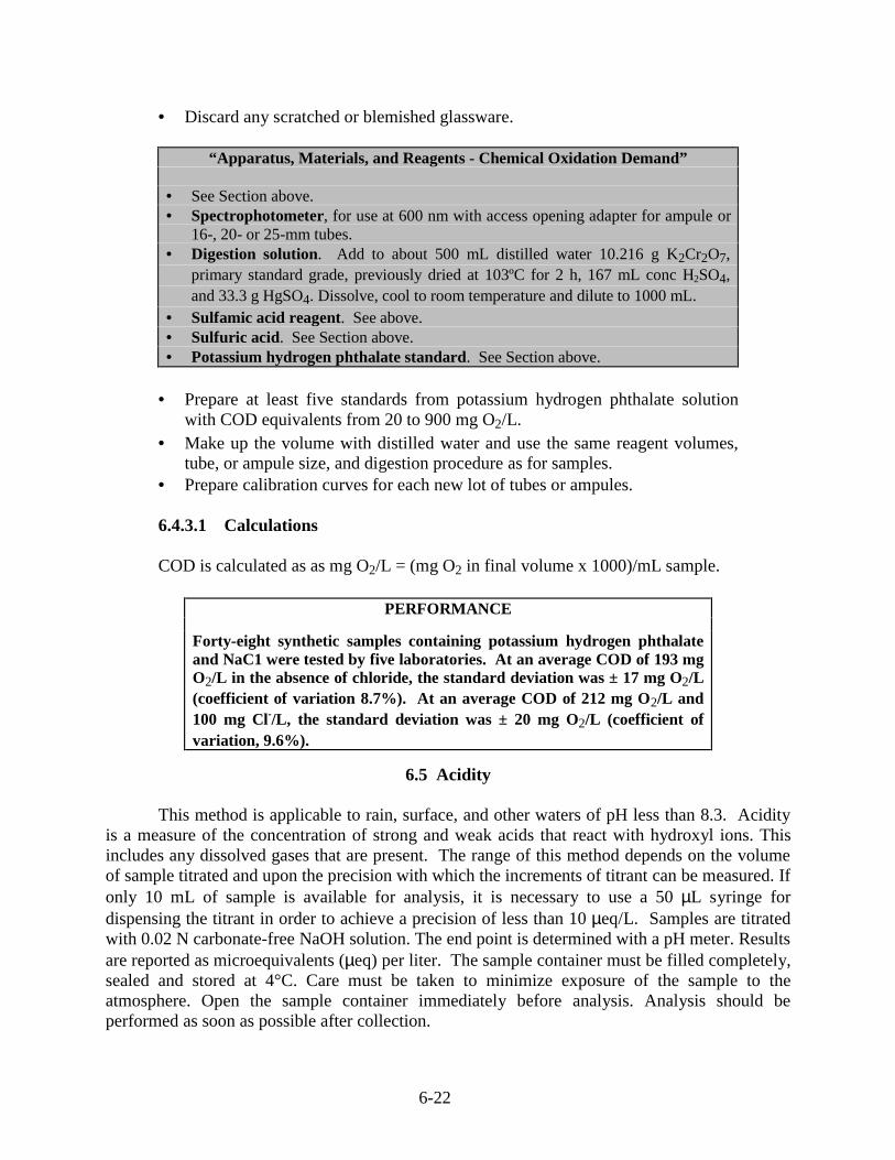
6-22

• Discard any scratched or blemished glassware.

“Apparatus, Materials, and Reagents - Chemical Oxidation Demand”

• See Section above.• Spectrophotometer, for use at 600 nm with access opening adapter for ampule or

16-, 20- or 25-mm tubes.• Digestion solution. Add to about 500 mL distilled water 10.216 g K2Cr2O7,

primary standard grade, previously dried at 103ºC for 2 h, 167 mL conc H2SO4,and 33.3 g HgSO4. Dissolve, cool to room temperature and dilute to 1000 mL.

• Sulfamic acid reagent. See above.• Sulfuric acid. See Section above.• Potassium hydrogen phthalate standard. See Section above.

• Prepare at least five standards from potassium hydrogen phthalate solutionwith COD equivalents from 20 to 900 mg O2/L.

• Make up the volume with distilled water and use the same reagent volumes,tube, or ampule size, and digestion procedure as for samples.

• Prepare calibration curves for each new lot of tubes or ampules.


COD is calculated as as mg O2/L = (mg O2 in final volume x 1000)/mL sample.

PERFORMANCE

Forty-eight synthetic samples containing potassium hydrogen phthalateand NaC1 were tested by five laboratories. At an average COD of 193 mgO2/L in the absence of chloride, the standard deviation was ± 17 mg O2/L(coefficient of variation 8.7%). At an average COD of 212 mg O2/L and100 mg Cl-/L, the standard deviation was ± 20 mg O2/L (coefficient ofvariation, 9.6%).

6.5 Acidity

This method is applicable to rain, surface, and other waters of pH less than 8.3. Acidityis a measure of the concentration of strong and weak acids that react with hydroxyl ions. Thisincludes any dissolved gases that are present. The range of this method depends on the volumeof sample titrated and upon the precision with which the increments of titrant can be measured. Ifonly 10 mL of sample is available for analysis, it is necessary to use a 50 µL syringe fordispensing the titrant in order to achieve a precision of less than 10 µeq/L. Samples are titratedwith 0.02 N carbonate-free NaOH solution. The end point is determined with a pH meter. Resultsare reported as microequivalents (µeq) per liter. The sample container must be filled completely,sealed and stored at 4°C. Care must be taken to minimize exposure of the sample to theatmosphere. Open the sample container immediately before analysis. Analysis should beperformed as soon as possible after collection.

6-23

The following method is adapted from: US EPA. 1998. Understanding EnvironmentalMethods: Analytical Methods, Environmental Analysis, and Data Evaluation: EPA Method305.2 (Test Method, December 1982); TITLE: Acidity (Titrimetric).© Genium PublishingCorporation 1996, Schenectady, NY 12304.

“Apparatus, Materials, and Reagents - Acidity”

• pH meter and electrode(s)• Micro buret or micro syringes.• Teflon or glass magnetic stirring bar.• Magnetic stirrer.• Beakers or flasks.• Standard sodium hydroxide solution, 1 N: Dissolve 40 g NaOH in 250 mL

distilled water. Cool and dilute to 1 liter with CO2 free distilled water. Store in apolyolefin bottle and fitted with a soda lime tube or tight cap to protect fromatmospheric CO2.

• Standard sodium hydroxide titrant, 0.02 N: Dilute 20.0 mL of 1 N NaOH withCO2-free distilled water to 1 liter. Store in rubber stoppered bottle. Protect fromatmospheric CO2 by using a soda lime tube. Standardize against an 0.02 Npotassium hydrogen phthalate solution prepared by dissolving 4.085 g ofanhydrous KHC8H4O4 in CO2-free distilled water and diluted to 1 L.

6.5.1 Sample Preparation and Processing

Samples with an initial pH between 4.3 and 8.3 are subject to error due to the loss or gainof dissolved gases during sampling, storage and analysis. To prepare and process a sample:

• Pipet an appropriate aliquot of sample into a beaker or flask containing asmall Teflon or glass stirring bar.

• Use extreme care to minimize the sample surface disturbance.• Immerse the pH electrode(s) into the sample and stir at a rate that does not

cause sample surface disturbance.• Titrate with 0.02 N NaOH to pH 8.3. Titration should be made as quickly as

possible to prevent absorption of atmospheric CO2.• Record the volume of the titrant.

6.5.2 Calculations

mL(B)

0.020 x mL(K) N(B) NaOH, ofNormality =

Acidity is calculated as µeq/L = (mL(B)/mL(s)) x N(B) x 106 where

µeq/L = microequivalents per litermL(K) = mL of KHC8H4O4

mL(B) = mL of NaOH titrantmL(s) = mL of sample

6-24

N(B) = normality of titrantPrecision and accuracy data are not available.

6.6 pH

This method is applicable to marine waters, freshwaters, and wastewaters. The pH of asample is determined electrometrically using either a glass electrode in combination with areference potential, a combination electrode or stainless steel probe with silicon chip sensor andtemperature sensor. Samples should be analyzed as soon as possible, preferably in the field atthe time of sampling.

“Apparatus, Materials, and Reagents - pH”

• pH Meter-laboratory or field model. A wide variety of instruments arecommercially available with various specifications and optional equipment.

• Glass electrode.• Reference electrode-a calomel, silver-silver chloride or other reference electrode

of constant potential may be used. NOTE: Combination electrodes incorporatingboth measuring and reference functions are convenient to use and are availablewith solid, gel type filling materials that require minimal maintenance.

• Magnetic stirrer and Teflon-coated stirring bar.• Thermometer or temperature sensor for automatic compensation.• Primary standard buffer salts are available from the National Institute of

Standards and Tests (NIST) and should be used in situations where extremeaccuracy is necessary. Preparation of reference solutions from these salts requiresome special precautions and handling, such as low conductivity dilution water,drying ovens, and carbon dioxide free purge gas. These solutions should bereplaced at least once each month.

• Secondary standard buffers may be prepared from NIST salts or purchased as asolution from commercial vendors. Use of these commercially available solutions,that have been validated by comparison to NIST standards, are recommended forroutine use.

• Because of the wide variety of pH meters and accessories, detailed operatingprocedures cannot be incorporated into this method. Each analyst must beacquainted with the operation of each system and familiar with all instrumentfunctions. Special attention to care of the electrodes is recommended.

• Each instrument/electrode system must be calibrated at a minimum of two pointsthat bracket the expected pH of the samples and are approximately three pH unitsor more apart. Various instrument designs may involve use of a “balance” or“standardize” dial and/or a slope adjustment as outlined in the manufacturer'sinstructions. Repeat adjustments on successive portions of the two buffer solutionsas outlined in procedure 8.2 until readings are within 0.05 pH units of the buffersolution value.

Glass electrodes, in general, are not subject to solution interferences from color, turbidity,colloidal matter, oxidants, reductants or high salinity. Coatings of oily material or particulatematter can impair electrode response. These coatings can usually be removed by gentle wiping ordetergent washing, followed by distilled water rinsing. An additional treatment with hydrochloricacid may be necessary to remove any remaining film. Temperature effects on the electrometricmeasurement of pH arise from two sources. The first is caused by a change in electrode output at

6-25

various temperatures. This interference can be controlled with instruments having temperaturecompensation or by calibrating the electrode-instrument system at the temperature of thesamples. The second source is the change of pH inherent in the sample at various temperatures.This error is sample dependent and cannot be controlled. It should therefore be noted byreporting both the pH and temperature at the time of analysis.

The following method is adapted from: US EPA Methods for Chemical Analysis ofWater and Wastes. Environmental Monitoring Systems Laboratory - Cincinnati ((EMSLCI),EPA-600/4-79-020, Revised March 1983 and 1979.


To prepare a sample for analysis:

• Standardize the meter and electrode system as instructed by the manufacturer.• Place the sample or buffer solution in a clean glass beaker using a sufficient

volume to cover the sensing elements of the electrodes and to give adequateclearance for the magnetic stirring bar.

• If field measurements are being made, the electrodes may be immerseddirectly in the sample stream to an adequate depth and moved in a manner toinsure sufficient sample movement across the electrode sensing element asindicated by drift free (< 0.1 pH) readings.

• If the sample temperature differs by more than 2ºC from the buffer solution,the measured pH values must be corrected.

• Instruments are equipped with automatic or manual compensators thatelectronically adjust for temperature differences. Refer to the manufacturer'sinstructions.

• After rinsing and gently wiping the electrodes, if necessary, immerse theminto the sample beaker or sample stream and stir at a constant rate to providehomogeneity and suspension of solids.

• The rate of stirring should minimize the air transfer rate at the air-waterinterface of the sample.

Note and record sample pH and temperature. Repeat the measurement on successive volumes ofsample until values differ by less than 0.1 pH units. Two or three volume changes are usuallysufficient.

6.6.2 Calculations

pH meters read directly in pH units. Report pH to the nearest 0.1 unit and temperature tothe nearest degree C.

PERFORMANCE

Forty-four analysts in twenty laboratories analyzed six synthetic watersamples containing exact increments of hydrogen hydroxyl ions, with thefollowing results:

6-26

Accuracy as pH Units Standard Deviation Bias, Bias, pH Units, % pHUnits

3.5 0.10 -0.29 -0.01

3.5 0.11 -0.00 -------7.1 0.20 +1.01 +0.077.2 0.18 -0.03 -0.0028.0 0.13 -0.12 -0.018.0 0.12 +0.16 +0.01

6.7 Conductivity

Conductivity is a measure of the ability of an aqueous solution to carry an electric currentand depends on the presence of ions (e.g., total concentration, mobility, and valence) and thetemperature of the measurements. Conductivity is a useful measurement to determine the degreeof mineralization (commonly called total dissolved solids) in water. This information is used todetermine the overall ionic effect of a water source and evaluate the potential for physiologicaleffects on plants and animals.

The following method is adapted from 18th Edition Standard Methods for theExamination of Water and Wastewater, Method 2510: Conductivity; Greenberg, A.E., Clesceri,L.S., and A.D. Eaton (eds), APHA: Washington, 1992.

“Apparatus, Materials, and Reagents - Conductivity”

• Self-Contained Conductivity Instruments. Use an instrument capable ofmeasuring conductivity with an error not exceeding 1% or 1 µmho/cm, whicheveris greater.

• Thermometer. Capable of being read to the nearest 0.1ºC and covering the range23 to 27ºC.

• Conductivity Cell:1. Platinum-electrode type. Conductivity cells containing platinized electrodes

are available in either pipet or immersion form. Cell choice depends onexpected range of conductivity. Experimentally check instrument bycomparing instrumental results with true conductivities of the KCl solutionslisted in the following table:

Equivalent Conductivity, Λ, and Conductivity, k, of Potassium Chloride at 25.0ºC*KCl Concentration Equivalent Conductivity, Conductivity, k,M or equivalent/L µmho-cm2/equivalent µmho/cm

0 149.90.0001 148.9 14.90.0005 147.7 73.90.001 146.9 146.90.005 143.6 717.50.01 141.2 1 412

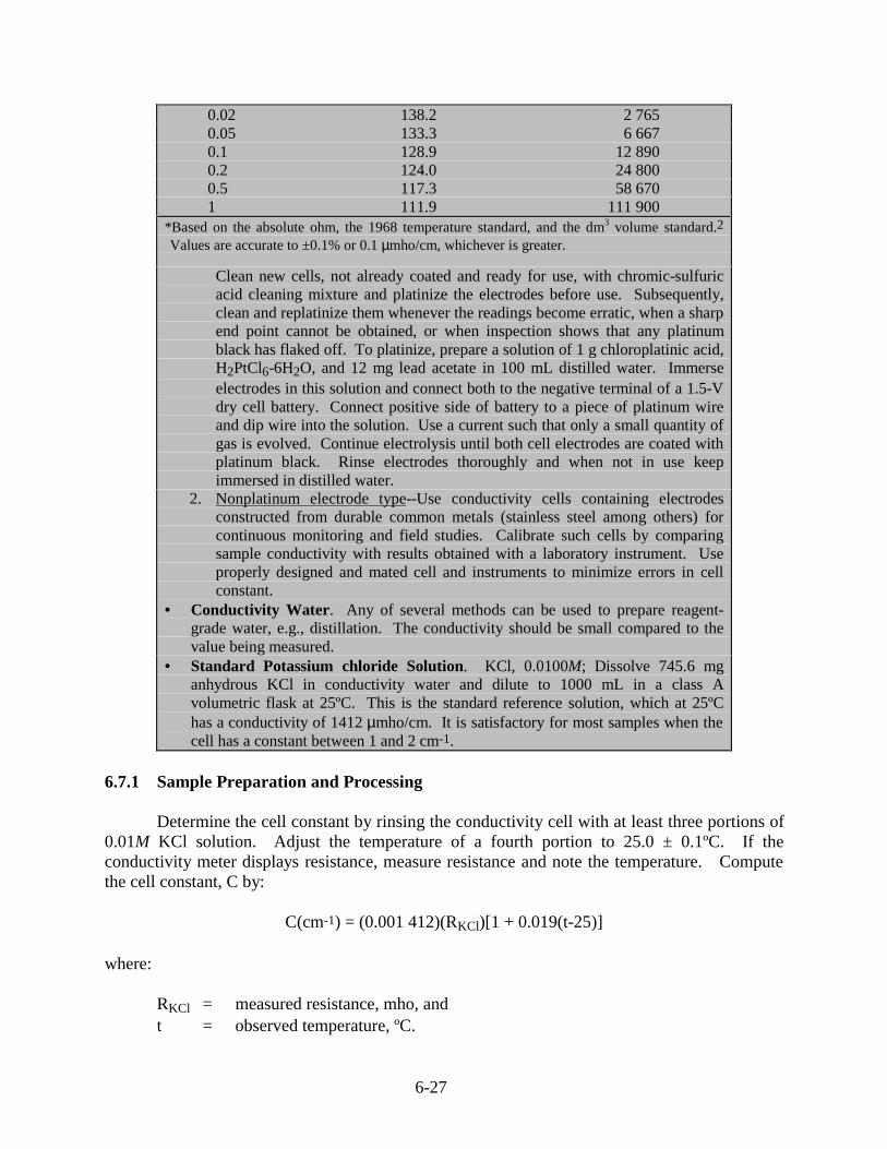
6-27

0.02 138.2 2 7650.05 133.3 6 6670.1 128.9 12 8900.2 124.0 24 8000.5 117.3 58 6701 111.9 111 900

*Based on the absolute ohm, the 1968 temperature standard, and the dm3 volume standard.2

Values are accurate to ±0.1% or 0.1 µmho/cm, whichever is greater.

Clean new cells, not already coated and ready for use, with chromic-sulfuricacid cleaning mixture and platinize the electrodes before use. Subsequently,clean and replatinize them whenever the readings become erratic, when a sharpend point cannot be obtained, or when inspection shows that any platinumblack has flaked off. To platinize, prepare a solution of 1 g chloroplatinic acid,H2PtCl6-6H2O, and 12 mg lead acetate in 100 mL distilled water. Immerseelectrodes in this solution and connect both to the negative terminal of a 1.5-Vdry cell battery. Connect positive side of battery to a piece of platinum wireand dip wire into the solution. Use a current such that only a small quantity ofgas is evolved. Continue electrolysis until both cell electrodes are coated withplatinum black. Rinse electrodes thoroughly and when not in use keepimmersed in distilled water.

2. Nonplatinum electrode type--Use conductivity cells containing electrodesconstructed from durable common metals (stainless steel among others) forcontinuous monitoring and field studies. Calibrate such cells by comparingsample conductivity with results obtained with a laboratory instrument. Useproperly designed and mated cell and instruments to minimize errors in cellconstant.

• Conductivity Water. Any of several methods can be used to prepare reagent-grade water, e.g., distillation. The conductivity should be small compared to thevalue being measured.

• Standard Potassium chloride Solution. KCl, 0.0100M; Dissolve 745.6 mganhydrous KCl in conductivity water and dilute to 1000 mL in a class Avolumetric flask at 25ºC. This is the standard reference solution, which at 25ºChas a conductivity of 1412 µmho/cm. It is satisfactory for most samples when thecell has a constant between 1 and 2 cm-1.


Determine the cell constant by rinsing the conductivity cell with at least three portions of0.01M KCl solution. Adjust the temperature of a fourth portion to 25.0 ± 0.1ºC. If theconductivity meter displays resistance, measure resistance and note the temperature. Computethe cell constant, C by:

C(cm-1) = (0.001 412)(RKCl)[1 + 0.019(t-25)]

where:

RKCl = measured resistance, mho, andt = observed temperature, ºC.

6-28

Conductivity meters often directly indicate conductivity. Commercial probes commonlycontain a temperature sensor. With such instruments, rinse the probe three times with 0.0100MKCl, as above. Adjust the temperature compensation dial to 0.0191ºC. With the probe instandard KCl solution, adjust the meter to read 1412 µmho/cm. this procedure automaticallyadjusts the cell constant internal to the meter.

To measure conductivity, rinse the cell with one or more portions of sample. Adjust thetemperature of a final portion of the sample to about 25.0ºC. Measure sample resistance orconductivity and note the temperature to ± 0.1ºC.

The temperature coefficient of most waters is only approximately the same as that of thestandard KCl solution. The more the temperature of the measurement deviates from 25ºC, thegreater the uncertainty in applying the temperature correction. Report all conductivities at25.0ºC.

6.7.2 Calculations

When sample resistance is measured, conductivity at 25ºC is:

)]t(.[R

)C)(,,(k

m 2501901

0000001

−+=

where:

k = conductivity, µmho/cm,C = cell constant, cm-1,Rm = measured resistance of sample, mho, andt = temperature of measurement.

When sample conductivity is measured without internal temperature compensationconductivity is:

25)0.0191(t1

)(khmo/cmk, m

−+=

where:

km = measured conductivity in units of µmho/cm at tºC, and other units are defined asabove.

For instruments with automatic temperature compensation and readout directly inµmho/cm or similar units, the readout is automatically corrected to 25ºC. Report the displayedconductivity in the designated units.

For instruments giving values in SI units,

1 mS/m = 10 µmho/cm, or conversely,1 µmho/cm = 0.1 mS/m.

6-29

PERFORMANCE

The precision of commercial conductivity meters is commonly between 0.1and 1.0%. Reproducibility of 1 to 2% is expected after an instrument hasbeen calibrated with such data shown in the table above.

6.8 Nitrate/Nitrite

Nitrogen is a required micronutrient for the growth of biological organisms. Theintroduction of nitrate into waters can cause a proliferation of biological organisms if nitrogen isnaturally limiting to growth. The two most important forms of nitrogen dissolved in water arenitrate and nitrite. Bacteria are capable of reducing nitrate to nitrite, so often the total nitrogenload is measured as a combination of these two species. Other forms of nitrogen are oftenpresent such as ammonia and organic nitrogen but these forms are generally less important thannitrate. Eutrophication induced by the discharge of excess nutrients to receiving waters caninfluence water quality. Eutrophication is caused by the consumption of dissolved oxygenduring the aerobic decomposition of the organic remains of organisms.

6.8.1 Spectrophotometric, Cadmium Reduction Method

This method can be applied to the determination of nitrite, or nitrite and nitrate combinedin marine waters, freshwater, and wastewaters and is adapted from EPA Method 353.3. Theapplicable range of this method is 0.01 to 1.0 mg/L nitrate-nitrite nitrogen. Samples with highconcentrations can be diluted to fall within the applicable range.

Apparatus, Materials, and Reagents for Nitrite/Nitrate

Reduction column: The column in Figure 6.1 was constructed from a 100 mL pipet byremoving the top portion. This column may also be constructed from two pieces oftubing joined end to end. A 10 cm length of 3 mm in diameter tubing is joined to a 25cm length of 3.5 mm inner diamter (ID) tubing or equivalent.Spectrophotometer for use at 540 nm, providing a light path of 1 cm or longer.Granulated cadmium: 40-60 mesh (MCB Reagents).Copper-Cadmium: The cadmium granules (new or used) are cleaned with dilute HCland copperized with 2% solution of copper sulfate in the following manner: 1) Washthe cadmium with dilute HCl and rinse with distilled water. The color of the cadmiumshould be silver. 2) Swirl 25 g cadmium in 100 mL portions of a 2% solution ofcopper sulfate for 5 minutes or until blue color partially fades, decant and repeat withfresh copper sulfate until a brown colloidal precipitate forms. 3) Wash the copper-cadmium with distilled water (at least 10 times) to remove all the precipitated copper.The color of the cadmium so treated should be black.Preparation of reaction column: Insert a glass wool plug into the bottom of thereduction column and fill with distilled water. Add sufficient copper-cadmium granulesto produce a column 18.5 cm in length. Maintain a level of distilled water above thecopper- cadmium granules to eliminate entrapment of air. Wash the column with 200mL of dilute ammonium chloride solution. The column is then activated by passingthrough the column 100 mL of a solution composed of 25 mL of a 1.0 mg/L NO3

-Nstandard and 75 mL of ammonium chloride-EDTA solution. Use a flow rate between7 and 10 mL per minute.Ammonium chloride- EDTA solution: Dissolve 13 g ammonium chloride and 1.7 gdisodium ethylenediamine tetraacetate in 900 mL of distilled water. Adjust the pH to

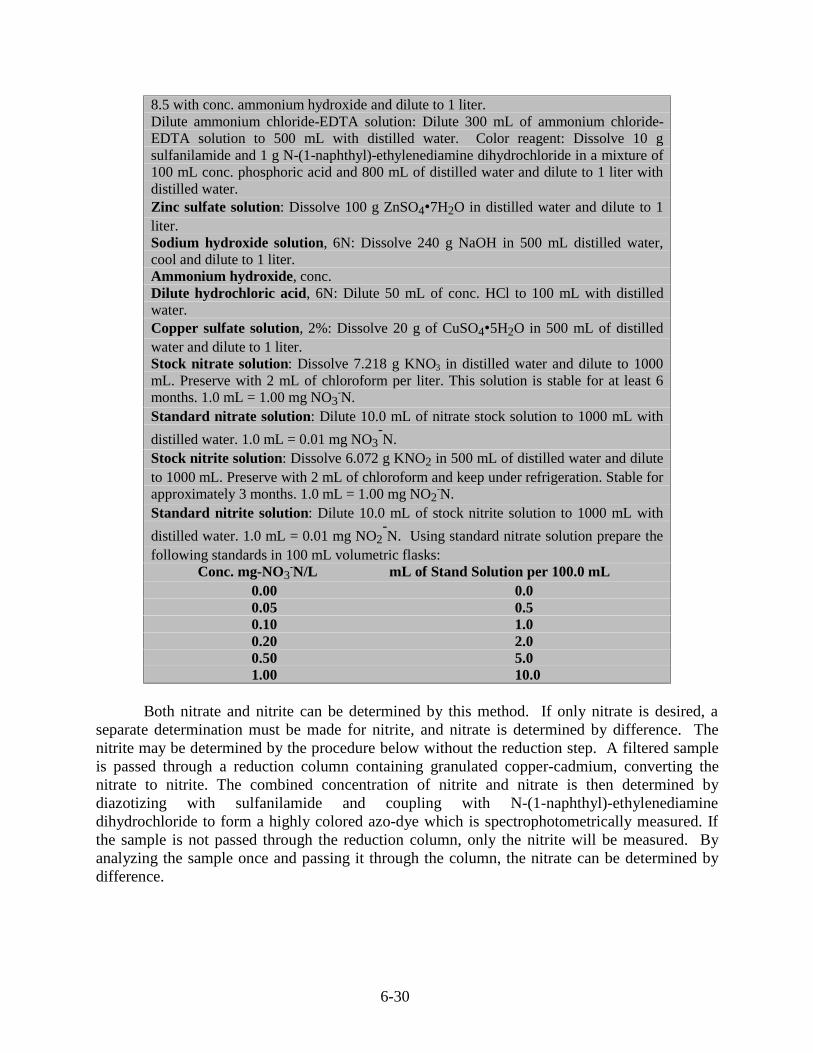
6-30

8.5 with conc. ammonium hydroxide and dilute to 1 liter.Dilute ammonium chloride-EDTA solution: Dilute 300 mL of ammonium chloride-EDTA solution to 500 mL with distilled water. Color reagent: Dissolve 10 gsulfanilamide and 1 g N-(1-naphthyl)-ethylenediamine dihydrochloride in a mixture of100 mL conc. phosphoric acid and 800 mL of distilled water and dilute to 1 liter withdistilled water.Zinc sulfate solution: Dissolve 100 g ZnSO4•7H2O in distilled water and dilute to 1liter.Sodium hydroxide solution, 6N: Dissolve 240 g NaOH in 500 mL distilled water,cool and dilute to 1 liter.Ammonium hydroxide, conc.Dilute hydrochloric acid, 6N: Dilute 50 mL of conc. HCl to 100 mL with distilledwater.Copper sulfate solution, 2%: Dissolve 20 g of CuSO4•5H2O in 500 mL of distilledwater and dilute to 1 liter.Stock nitrate solution: Dissolve 7.218 g KNO3 in distilled water and dilute to 1000mL. Preserve with 2 mL of chloroform per liter. This solution is stable for at least 6months. 1.0 mL = 1.00 mg NO3

-N.Standard nitrate solution: Dilute 10.0 mL of nitrate stock solution to 1000 mL with

distilled water. 1.0 mL = 0.01 mg NO3-N.

Stock nitrite solution: Dissolve 6.072 g KNO2 in 500 mL of distilled water and diluteto 1000 mL. Preserve with 2 mL of chloroform and keep under refrigeration. Stable forapproximately 3 months. 1.0 mL = 1.00 mg NO2

-N.Standard nitrite solution: Dilute 10.0 mL of stock nitrite solution to 1000 mL with

distilled water. 1.0 mL = 0.01 mg NO2-N. Using standard nitrate solution prepare the

following standards in 100 mL volumetric flasks:Conc. mg-NO3

-N/L mL of Stand Solution per 100.0 mL0.00 0.00.05 0.50.10 1.00.20 2.00.50 5.01.00 10.0

Both nitrate and nitrite can be determined by this method. If only nitrate is desired, aseparate determination must be made for nitrite, and nitrate is determined by difference. Thenitrite may be determined by the procedure below without the reduction step. A filtered sampleis passed through a reduction column containing granulated copper-cadmium, converting thenitrate to nitrite. The combined concentration of nitrite and nitrate is then determined bydiazotizing with sulfanilamide and coupling with N-(1-naphthyl)-ethylenediaminedihydrochloride to form a highly colored azo-dye which is spectrophotometrically measured. Ifthe sample is not passed through the reduction column, only the nitrite will be measured. Byanalyzing the sample once and passing it through the column, the nitrate can be determined bydifference.

6-31


Analysis should be performed as soon as possible. If the analysis cannot be made within24 hours, the sample should be preserved with sulfuric acid (2 mL H2SO4 per liter) andrefrigerated at 4ºC. However, once preserved, only nitrate + nitrite can be determined.Otherwise store refrigerated at 4ºC. Samples to be analyzed for nitrate with the reductioncolumn must not be preserved with mercuric chloride. Interferences can come from severalsources. Flow through the reduction column can be reduced due to build up of suspended matter.This is easily controlled by pre-filtering through a glass fiber filter or a 0.45 µm membrane filter.If samples are highly turbid samples, they may be pretreated with zinc sulfate before filtration toremove the bulk of particulate matter present in the sample. Samples containing highconcentrations of iron, copper and other metals may be underestimated. A pre-treatment ofEDTA can reduce the interference. Samples that contain large concentrations of oil and greasewill coat the surface of the cadmium and reduce the efficiency of the reduction step. Pre-extraction of the sample with an organic solvent will reduce the effects on the reduction step.

Removal of turbidity is accomplished by filtration of the sample or in severe casesthrough flocculation and subsequent filtering. Filter the sample through a glass fiber filter or a0.45 µm membrane filter. For samples with high levels of suspended matter, add 1 mL zincsulfate solution to 100 mL of sample and mix thoroughly. Add 0.4-0.5 mL sodium hydroxidesolution to obtain a pH of 10.5 as determined with a pH meter. Let the treated sample stand afew minutes to allow the heavy flocculent to precipitate and settle. Clarify the sample byfiltering it through a glass fiber filter or a 0.45 µm membrane filter.

Oil and grease removal is accomplished by a quick solvent extraction technique. Adjustthe pH of 100 mL of filtered sample to 2 by addition of conc. HCl. Extract the oil and greasefrom the aqueous solution with two 25 mL portions of a non-polar solvent (i.e., chloroform orequivalent).


The pH should be adjusted if the sample pH is below 5 or above 9 with either conc. HClor conc. NH4OH. This is done to insure a sample pH of 8.5 after the following step. To 25.0 mLof sample or an aliquot diluted to 25.0 mL, add 75 mL of ammonium chloride-EDTA solutionand mix. Then,

• Pour the sample into the column and collect the sample at a rate of 7-10 mLper minute.

• Discard the first 25 mL, collect the rest of the sample (approximately 70 mL)in the original sample flask.

• Reduced samples should not be allowed to stand longer than 15 minutesbefore addition of color reagent.

• Add 2.0 mL of color reagent to 50.0 mL of sample.• Allow 10 minutes for color development.• Within 2 hours measure the absorbance at 540 nm against a reagent blank.

6-32

NOTE: If the concentration of sample exceeds 1.0 mg NO3-N/L, the remainder of the reduced

sample may be used to make an appropriate dilution before proceeding with the next step. Carryout the reduction of standards exactly as described for the samples.

At least one nitrite standard should be compared to a reduced nitrate standard at the sameconcentration to verify the efficiency of the reduction column.


Obtain a standard curve by plotting the absorbance of standards run by the above

procedure against NO3-N mg/L. Compute concentration of samples by comparing sample

absorbance with standard curve. If less than 25 mL of sample is used for the analysis, thefollowing equation should be used:

NO2 + NO3 (mg N/L) = (A x 25)/mL sample used

where:

A = Concentration of nitrate from the standard curve.

6.8.2 Autoanalyzer Method

The following procedure is used to determine nitrite singly or nitrite and nitrate combinedin fresh, saline, or wastewater. The applicable concentration range for this method is 0.05 to10.0 mg/L nitrate-nitrite nitrogen. The concentration range may be extended by dilution of thesample. In this procedure, a filtered sample is passed through a column containing granulatedcopper-cadmium to reduce nitrate to nitrite. The nitrite (that originally present plus reducednitrate) is determined by diazotizing with sulfanilamide and coupling with N-(1-naphthyl)-ethylenediamine dihydrochloride to form a highly colored azo dye which is colorimetricallymeasured. Speciated, rather than combined nitrate-nitrite, values are readily obtained bycarrying out the procedure first with, and then without, the Cu-Cd reduction step.


Analysis should be completed as soon as possible after collection. If analyses can beconducted within 24 hours, the sample should be preserved by refrigeration at 4°C.

“Apparatus, Materials, and Reagents - Nitrate/Nitrite”

• Technicon or Equivalent AutoAnalyzer (AAI or AAII) consisting of thefollowing components:

- Sampler- Manifold (AAI) or analytical cartridge (AAII).- Proportioning Pump- Colorimeter equipped with a 15 mm or 50 mm tubular flow cell and 540 nm

filters.- Recorder- Digital printer.

• Granulated cadmium: 40-60 mesh (take extreme care in handling metalliccadmium, it is very toxic).

6-33

• Copper-cadmium. The cadmium granules (new or used) are cleaned with diluteHCl and copperized with 2% solution of copper sulfate in the following manner:

- Wash the cadmium with HCl and rinse with distilled water. The color of thetreated cadmium should be silver.

- Swirl 10 g cadmium in 100 mL portions of 2% solution of copper sulfate forfive minutes or until the blue color partially fades, decant and repeat with freshcopper sulfate until a brown colloidal precipitate forms.

- Wash the cadmium-copper with distilled water (at least 10 times) to remove allof the precipitated copper. The color of the treated cadmium should be black.

• Preparation of reduction column AAI: The reduction column is an 8 by 50 mmglass tube with the ends reduced in diameter to permit insertion into the system.Copper-cadmium granules are placed in the column between glass wool plugs. Thepacked reduction column is placed in an up-flow 20° incline to minimizechanneling (Figure 6.1).

• Preparation of reduction column: The reduction column is a U-shaped, 35 cmlength, 2 mm I.D. glass tube (Note 1). Fill the reduction column with distilledwater to prevent entrapment of air bubbles during the filling operations. Transferthe copper-cadmium granules to the reduction column and place a glass wool plugin each end. To prevent entrapment of air bubbles in the reduction column be surethat all pump tubes are filled with reagents before putting the column into theanalytical system.NOTE 1: A 0.081 I.D. pump tube (purple) can be used in place of the 2 mm

glass tube.• Distilled water. Because of possible contamination, distilled water should be

prepared by passing it through an ion exchange column comprised of a mixture ofboth strongly acidic-cation and strongly basic-anion exchange resins. Theregeneration of the ion exchange column should be carried out according to themanufacturer's instructions or Type I water by CAP/NCCLS.

• Color reagent. Add while stirring, 100 mL conc. phosphoric acid, 40 gsulfanilamide, and 2 g N-1-naphthylethylenediamine dihydrochloride to 800 mL ofdistilled water. Stir until all materials dissolve and then dilute to 1 liter. Store in abrown bottle and keep in the dark when not in use. This solution is stable forseveral months.

• Dilute hydrochloric acid, 6N: Dilute 50 mL of conc. HCl to 100 mL with distilledwater.

• Copper sulfate solution, 2%: Dissolve 20 g of CuSO4•5H2O in 500 mL ofdistilled water and dilute to 1 liter.

• Wash solution. Use distilled water for unpreserved samples. For samplespreserved with H2SO4, use 2 mL H2SO4 per liter of wash water.

• Ammonium chloride-EDTA solution. Dissolve 85 g of reagent grade ammonium

Figure 6.1. Copper Cadmium Reduction Column.

6-34

chloride and 0.1 g of disodium ethylenediamine tetraacetate in 900 mL of distilledwater. Adjust the pH to 8.5 with conc. ammonium hydroxide and dilute to 1 liter.Add 1/2 mL Brij-35 (available from Technicon Corporation).

• Stock nitrate solution. Dissolve 7.218 g KNO3 and dilute to 1 liter in avolumetric flask with distilled water. Preserve with 2 mL of chloroform per liter.This solution is stable for 6 months (1 mL = 1.0 mg NO3

-N).• Stock nitrite solution. Dissolve 6.072 g KNO2 in 500 mL of distilled water and

dilute to 1 liter in a volumetric flask. Preserve with 2 mL of chloroform and keeprefrigerated (1.0 mL = 1.0 mg NO2

-N).• Standard nitrate solution. Dilute 10.0 mL of stock nitrate solution to 1000 mL.

1.0 mL = 0.01 mg NO3-N. Preserve with 2 mL of chloroform per liter. Solution is

stable for 6 months.• Standard nitrite solution. Dilute 10.0 mL of stock nitrite solution to 1000 mL.

1.0 mL = 0.01 mg NO2-N. Solution is unstable; prepare as required.

• Using the standard nitrate solution, prepare the following standards in 100.0 mLvolumetric flasks. At least one nitrite standard should be compared to a nitratestandard at the same concentration to verify that the reduction column is efficientlyoperating.

Conc., mgNO,-N or NO3-N/L mL Standard Solution/100 mL

0.0 00.05 0.50.10 1.00.20 2.00.50 5.0

1.00 10.02.00 20.04.00 40.06.00 60.0

When the samples to be analyzed are saline waters, Substitute Ocean Water (SOW)should be used for preparing the standards; otherwise, distilled water is used. Thecomposition of SOW is:

NaCl - 24.53 g/L MgCl2 - 5.20 g/L Na2SO4 - 4.09 g/LCaCl2 - 1.16 g/L KCl - 0.70 g/L NaHCO3 - 0.20 g/LKBr - 0.10 g/L H3BO3 - 0.03 g/L SrCl2 - 0.03 g/LNaF - 0.003 g/L


If the pH of the sample is below 5 or above 9, adjust the pH to between 5 and 9 witheither concentrated HCl or concentrated NH4OH. Set up the manifold as shown in Figure 6.2(AAI) or Figure 6.3 (AAII). Note that reductant column should be in 20º incline position (AAI).Care should be taken not to introduce air into the reduction column on the AAII. Allow bothcolorimeter and recorder to warm up for 30 minutes. Obtain a stable baseline with all reagents,flushing distilled water through the sample line. Condition the column by flushing 1 mg/Lstandard for 10 minutes when a new reduction column is first used. Subsequently wash thecolumn with reagents for 20 minutes.

6-35

Figure 6.2. Nitrate-Nitrite Manifold AA-I.

Figure 6.3. Nitrate-Nitrite Manifold AA-II.

6-36

Place the appropriate nitrate and/or nitrite standards in the sampler in order of increasingconcentration of nitrogen. Complete loading of sampler tray with unknown samples and beginanalyses.


Prepare appropriate standard curve or curves derived from the NO2-N and/or NO3

-Nstandards. Compute the concentration of samples by comparing sample peak heights with thestandard curve.

The analyst should be aware that interferences with the method can be caused by anumber of factors:

• The build-up of suspended matter in the reduction column will restrictsample flow. Since nitrate-nitrogen is dissolved, the sample may bepre-filtered.

• Low results may be obtained for samples that contain highconcentrations of iron, copper or other metals. EDTA is added to thesamples to eliminate this interference.

• Samples that contain large concentrations of oil and grease will coatthe surface of the cadmium. This interference is eliminated by pre-extracting the sample with an organic solvent.

Autoanalyzer methods are also available for other nutrients. The analyst should consultthe manufacturers’ manual.

6.8.3 Portable Test Kits

There are portable test kits available for the nitrate/nitrite analysis that provide pre-packaged reagents that limit the necessity for large equipment purchases and limit the amount ofchemical waste generated. This technique utilizes cadmium to reduce nitrates to nitrite in thesample, the nitrate reacts with sulfanilic acid in an acidic medium to form an intermediatediazonium salt. The absorbance at 500 nm is determined using either a calibrated bench orportable spectrophotometer. The working range for this method is 0 to 30.0 mg/L NO3-N. Themethod is as follows:

“Apparatus, Materials, and Reagents - Nitrate/Nitrite”

• Portable or bench spectrophotometer with 500 nm filter (HACH 800 or similar Cat.No. 48470-00) or equivalent.

• Sample cells• Bromine Water• Nitrate Nitrogen Standard• Phenol Solution• Graduated cylinder• Sodium Hydroxide

6-37

• Deionized Water• Prepackaged Reagents• Stopwatch

• Fill sample cell with 10 or 25 mL of sample (depending on instrument).• Add pre-packaged reagent to the cell, stopper the cell.• Shake for one minute.• Add bromine water (30 g/L) dropwise to the sample until a yellow color

remains.• Add one drop of phenol solution (30 g/L), to remove color.• Time reaction, 5 minutes.• Fill another cell with 10 or 25 mL of sample (depending on instrument) as

instrument blank.• Zero instrument using instrument blank.• Take sample reading.

The samples can be stored for up to 14 days at a pH equal to 2 (adjusted using sulfuricacid), in the dark, and refrigerated. Before analyzing stored samples, samples will need to beneutralized using sodium hydroxide. Strong oxidizing and reducing agents will interfere with theanalysis. Ferric iron will bias the results high while chloride greater than 100 mg/L will bias theresults low. The samples can also be analyzed using a color wheel to compare colors instead of aspectrophotometer; however; at least 20% more variability is introduced into the method. Pre-packaged portable laboratories are commercially available for a suite of water qualitymeasurements that can be performed in the field. The analyses that can be performed with thesetype of pre-packaged field kits include acidity, alkalinity, aluminum, ammonia, carbon dioxide,chloride, chlorine dioxide, color, conductivity, copper, hardness, total iron, manganese, dissolvedoxygen, pH, phosphate, silicate, sulfate, sulfide, suspended solids, temperature, turbidity andzinc.

6.8.4 Ion Selective Electrodes

Nitrate and nitrite concentrations can be measured by ion-selective electrode (ISE). Themain advantage of electrode technology is the specificity and the speed that an analysis can bemade. The electrode is immersed into the sample solution and the sample concentration isdirectly read on a specific ion meter or from a calibration curve. Time-consuming samplepreparation steps such as filtration and chromium addition are unnecessary. Sample color orturbidity does not affect the measurements. Analysis time is typically under one minute. TheISE is connected to a either a benchtop or portable Ion Selective Meter and the meter iscalibrated using calibration solutions. Nitrate and nitrite ions are measured using separatecombination plastic membrane electrodes. The working range for a nitrate ISE is from 0.1 to14,000 ppm and for a nitrite ISE is from 0.02 to 100 ppm. Samples should be analyzed as soonas possible, preferably in the field at the time of sampling.

“Apparatus, Materials, and Reagents - Ion Selective Electrodes”

• Ion Selective/pH Meter (similar to PCM700 ORION)• Nitrate Combination ISE (ORION 9707BN)

6-38

• Nitrite Combination ISE (ORION 9746BN)• Sample container• Nitrate Standards• Electrode filling Solution

There are numerous applications for ISE for the measurement of a large suite of analytes.Ion selective electrodes are used to serve as endpoint indicators for titrations for analytesincluding: aluminum, arsenic, azide, boron, chloride, chromium, iron, lithium, manganese,nickel, nitroloacetate, sulfate, and sulfur. The results using ISE as an indicator for analysesinvolving titrations are approximately ten times more precise than direct measurements, but moretime consuming. Direct measurements made with ion selective electrodes, where the probe isimmersed in the sample, is a very convenient field method. The meter is typically calibrated bymeasurement of a series of standards and the sample reading taken so that it is within thestandard curve. Samples with readings outside the standard curve would require an appropriatedilution to put the response within the calibration curve. Analytes suitable for directmeasurement include: ammonia, calcium, carbon dioxide, chloride, copper (with std addition),cyanide, fluoride, potassium, silver, sodium, and sulfide. Each ISE will have specific storagerequirements (e.g. soaking in low level standard, buffer, etc) for between samples, short-termstorage (up to one week), and long-term storage. The manufacturer can provide information onrange of operation, storage requirements, and method documentation.

6.8.5 Test Strips

Water quality test strips are commercially available (HACH Cat. No. 27454-25, ORIONCat No. T2080P or equivalent) for performing semi-quantitative nitrate/nitrite determinations.The test strips provide two reagent pads (for both nitrate and nitrite) on a single test strip. Thesetest strips give fast and reliable results that are very cost effective and eliminate the need forclean up or disposal of waste chemicals often associated with the classical wet chemical methodsdescribed above. The procedure for using these strips follows:

• The test strip is dipped into the sample.• Wait for the color to develop• Compare the color of the reagent pads to the color chart provided with the test

strips for the nitrate and nitrite concentration.

The range for NO3-N is 0 to 50 mg/L (with increments of 0, 1, 2, 5, 10, 20, and 50 mg/Lfor HACH) or 0 to 500 mg/L (with increments of 0, 10, 25, 50, 100, 250, 500 mg/L for ORION).For NO2-N the range is 0 to 3 ppm (with increments of 0, 0.15, 0.3, 1.0, 1.5, and 3.0 for HACH)and 0 to 80 (with increments of 0, 1, 5, 10, 25, 40, and 80 mg/L for ORION). This technique isbest suited to distinguish between large differences in nitrate/nitrite concentrations that would betypically encountered when determining the spatial distribution around a sewage outfall and notdefining fine scale variability. Test strips are also commercially available for the determinationof total alkalinity (0-240 mg/L), free and total chlorine (0-10 mg/L), total hardness (0-425 mg/L),total iron (0-5 mg/L), total copper (0-3 mg/L), ammonia (0-6 mg/L), and phosphate (0-50 mg/L).

6-39

6.9 Phosphate

Phosphorous is an additional essential micronutrient for biological organisms. As withnitrogen, the introduction of phosphorous into waters where it is growth-limiting can cause aproliferation of biological production contributing to eutrophication. Dissolved phosphorous isprimarily in the form of phosphate.

“Apparatus, Materials, and Reagents - Phosphate”

• Photometer. A spectrophotometer or filter photometer suitable for measurementsat 650 or 880 nm with a light path of 1 cm or longer.

• Acid-washed glassware. All glassware used should be washed with 1:1 HCl andrinsed with distilled water. The acid-washed glassware should be filled withdistilled water and treated with all the reagents to remove the last traces ofphosphorus that might be adsorbed on the glassware. Preferably, this glasswareshould be used only for the determination of phosphorus and after use it should berinsed with distilled water and kept covered until needed again. If this is done, thetreatment with 1:1 HCl and reagents is only required occasionally. Commercialdetergents should never be used.

• Sulfuric acid solution, 5N: Dilute 70 mL of concentrated H2SO4 with distilledwater to 500 mL.

• Antimony potassium tartar solution. Weigh 1.3715 g K(SbO)C4H4O6•1/2H2Odissolve in 400 mL distilled water in 500 mL volumetric flask, dilute to volume.Store at 4ºC in a dark, glass-stoppered bottle.

• Ammonium molybdate solution. Dissolve 20 g (NH4)6Mo7O24•4H2O in 500 mLof distilled water. Store in a plastic bottle at 4ºC.

• Ascorbic acid, 0.1 M: Dissolve 1.76 g of ascorbic acid in 100 mL of distilledwater. The solution is stable for about a week if stored at 4ºC.

• Combined reagent. Mix the above reagents in the following proportions for 100mL of the mixed reagent: 50 mL of 5N H2SO4, 5 mL of antimony potassiumtartrate solution, 15 mL of ammonium molybdate solution and 30 mL of ascorbicacid solution. Mix after addition of each reagent. All reagents must reach roomtemperature before they are mixed and must be mixed in the order given. Ifturbidity forms in the combined reagent, shake and let stand for a few minutes untilthe turbidity disappears before proceeding. Since the stability of this solution islimited, it must be freshly prepared for each run.

• Sulfuric acid solution, 11 N: Slowly add 310 mL conc. H2SO4 to 600 mL distilledwater. When cool, dilute to 1 liter.

• Stock phosphorus solution. Dissolve in distilled water 0.2197 g of potassiumdihydrogen phosphate, KH2PO4, which has been dried in an oven at 105ºC. Dilutethe solution to 1000 mL; 1.0 mL = 0.05 mg PO4-P.

• Standard phosphorus solution. Dilute 10.0 mL of stock phosphorus solution to1000 mL with distilled water; 1.0 mL=0.5 µg PO4-P. Using standard solution,prepare the following standards in 50.0 mL volumetric flasks:

mL of Standard Phosphorus Solution Conc., mg/L0 0.001.0 0.013.0 0.03

6-40

5.0 0.0510.0 0.1020.0 0.2030.0 0.3040.0 0.4050.0 0.50

• Sodium hydroxide, 1 N: Dissolve 40 g NaOH in 600 mL distilled water. Cooland dilute to 1 liter.

The reaction that forms the basis for this analysis is that of orthophosphate with antimonyand molybdate to produce an antimony-phospho-molybdate complex. Depending on thepretreatment of the sample, the various forms of phosphorus may be determined. The mostcommonly measured forms are phosphorus and dissolved phosphorus and orthophosphate anddissolved orthophosphate. Hydrolyzable phosphorus is normally found only in sewage-typesamples and the insoluble forms of phosphorus are determined by calculation. The concentrationrange for this method is between 0.01 to 1.2 mg PO4-P.

This method can be used for the determination of phosphorus in drinking, surface andsaline waters, domestic and industrial wastes and is adapted from EPA Method 365.2.


Samples can be collected in either clean plastic or glass containers. If analysis can not beperformed within 24 hours, the sample should be preserved with 2.0 mL of concentrated H2SO4per liter of sample and refrigerated at 4ºC. Various forms of phosphorus can be determinedusing different pretreatments.

For total phosphorus determinations:

• Add 1 mL of H2SO4 solution to a 50 mL sample in a 125 mL Erlenmeyerflask.

• Add 0.4 g of ammonium persulfate.• Boil gently on a pre-heated hot plate for approximately 30 minutes or until a

final volume of about 10 mL is reached.• Do not allow sample to go to dryness.

Alternatively:

• Heat for 30 minutes in an autoclave at 121ºC (15-20 psi).• Cool and dilute the sample to about 30 mL and adjust the pH of the sample to

7.0 ± 0.2 with 1 N NaOH (7.10) using a pH meter.• If the sample is not clear at this point, add 2-3 drops of acid and filter. Dilute

to 50 mL.

For hydrolyzable phosphorus determinations:

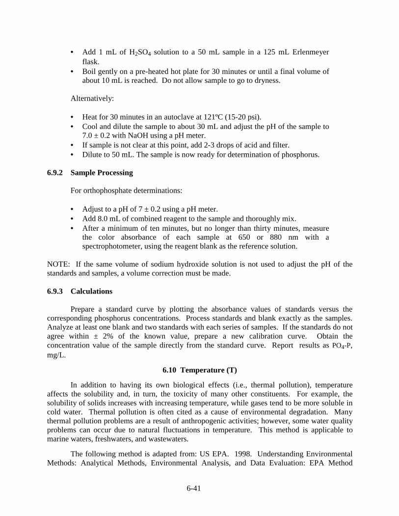
6-41

• Add 1 mL of H2SO4 solution to a 50 mL sample in a 125 mL Erlenmeyerflask.

• Boil gently on a pre-heated hot plate for 30 minutes or until a final volume ofabout 10 mL is reached. Do not allow sample to go to dryness.

Alternatively:

• Heat for 30 minutes in an autoclave at 121ºC (15-20 psi).• Cool and dilute the sample to about 30 mL and adjust the pH of the sample to

7.0 ± 0.2 with NaOH using a pH meter.• If sample is not clear at this point, add 2-3 drops of acid and filter.• Dilute to 50 mL. The sample is now ready for determination of phosphorus.


For orthophosphate determinations:

• Adjust to a pH of 7 ± 0.2 using a pH meter.• Add 8.0 mL of combined reagent to the sample and thoroughly mix.• After a minimum of ten minutes, but no longer than thirty minutes, measure

the color absorbance of each sample at 650 or 880 nm with aspectrophotometer, using the reagent blank as the reference solution.

NOTE: If the same volume of sodium hydroxide solution is not used to adjust the pH of thestandards and samples, a volume correction must be made.

6.9.3 Calculations

Prepare a standard curve by plotting the absorbance values of standards versus thecorresponding phosphorus concentrations. Process standards and blank exactly as the samples.Analyze at least one blank and two standards with each series of samples. If the standards do notagree within ± 2% of the known value, prepare a new calibration curve. Obtain theconcentration value of the sample directly from the standard curve. Report results as PO4-P,mg/L.

6.10 Temperature (T)

In addition to having its own biological effects (i.e., thermal pollution), temperatureaffects the solubility and, in turn, the toxicity of many other constituents. For example, thesolubility of solids increases with increasing temperature, while gases tend to be more soluble incold water. Thermal pollution is often cited as a cause of environmental degradation. Manythermal pollution problems are a result of anthropogenic activities; however, some water qualityproblems can occur due to natural fluctuations in temperature. This method is applicable tomarine waters, freshwaters, and wastewaters.

The following method is adapted from: US EPA. 1998. Understanding EnvironmentalMethods: Analytical Methods, Environmental Analysis, and Data Evaluation: EPA Method

6-42

170.1 Approved for NPDES (Issued 1974); TITLE: Temperature (Thermometric). © GeniumPublishing Corporation 1996, Schenectady, NY 12304.

Temperature measurements may be made with any good grade of mercury-filled or dial-type centigrade thermometer, or a thermistor. Measurement device should be routinely checkedagainst a certified precision thermometer.

PERFORMANCE

Precision and accuracy for this method have not been determined. Theprocedure to be used for this determination is found in: StandardMethods for the Examination of Water and Wastewater, 14th Edition, p.125, Method 212 (1975).

6.11 Coliform Bacteria

The membrane filter method can be applied for the determination and enumeration of thecoliform bacteria in freshwater, marine waters, and wastewaters. A membrane filter is placed onthe specified mEI agar medium and incubated at 41ºC for 24 h. Using magnification and afluorescent lamp, coliform are identified as those bacteria that produce colonies with a blue haloafter incubation on mEI agar. The presence of coliform in water is an indication of fecalpollution and the presence of enteric pathogens, and shows a direct relationship between thecoliform density in water and waste discharges. Measurement of living bacteria requiressubstantial infrastructure support and may not be able to be performed at locations with littleinfrastructure.


Sample preservation procedures and holding time limits must be carefully followed toproduce valid data. Bacteriological samples must be refrigerated at a temperature of 1-4ºCduring transit to the laboratory. Insulated containers assure proper maintenance of storagetemperature. Sample bottles should not be immersed in water during transit or storage.

Examine samples as soon as possible after collection. Do not hold samples longer than6 hours between collection and the initiation of the analyses.

“Apparatus, Materials, and Reagents - Coliform Bacteria”

• Glass lens with magnification of 2-5X or stereoscopic microscope.• Lamp, with a cool, white fluorescent tube.• Hand tally or electronic counting device.• Pipet container, stainless steel, aluminum or borosilicate glass, for glass pipets.• Pipets, sterile, bacteriological or Mohr, glass or plastic, of appropriate volume.• Graduated cylinders, 100-1000 mL, covered with aluminum foil or kraft paper

and sterile.• Membrane filtration units (filter base and funnel), glass, plastic or stainless steel,

wrapped with aluminum foil or kraft paper and sterile.• Ultraviolet unit for sanitization of the filter funnel between filtrations

(optional).

6-43

• Line vacuum, electric vacuum pump, or aspirator for use as a vacuum source.In an emergency or in the field, a hand pump or a syringe equipped with a checkvalve to prevent the return flow of air, can be used.

• Flask, filter, vacuum, usually 1 L, with appropriate tubing. A filter manifold tohold a number of filter bases is optional.

• Flask for safety trap placed between the filter flask and the vacuum source.• Forceps, straight or curved, with smooth tips to handle filters without damage.• Ethanol, methanol or isopropanol in a small, wide-mouth container, for

flame-sterilizing forceps.• Burner, Bunsen or Fisher type, or electric incinerator unit for sterilizing loops

and needles.• Thermometer, checked against a National Institute of Standards and Technology

(NIST) certified thermometer, or one that meets the requirements of NISTMonograph SP 250-23.

• Petri dishes, sterile, plastic, 50 x 12 mm, with tight-fitting lids.• Bottles, milk dilution, borosilicate glass, screw-cap with neoprene liners,

marked at 99 mL for 1-100 dilutions. Dilution bottles marked at 90 mL or tubesmarked at 9 mL may be used for 1-10 dilutions.

• Flasks, borosilicate glass, screw-cap, 250-2000 mL volume.• Membrane filters, sterile, white, grid marked, 47 mm diameter, with 0.45 + 0.02

µm pore size.• Inoculation loops, at least 3-mm diameter, and needles, nichrome or platinum

wire, 26 B & S gauge, in suitable holders.• Incubator maintained at 41 ± 0.5ºC.• Waterbath maintained at 44-46ºC for tempering agar.• Test tubes, 150 x 20 mm, borosilicate glass or plastic.• Caps, aluminum or autoclavable plastic, for 20 mm diameter test tubes.• Test tubes, screw-cap, borosilicate glass, 125 x 16 mm or other appropriate size.• Purity of Reagents. Reagent grade chemicals shall be used in all tests. The agar

used in preparation of culture media must be of microbiological grade. Wheneverpossible, use commercial culture media as a means of quality control.

• Purity of Water. Reagent water conforming to Specification D1193, Reagentwater conforming Type II, Annual Book of ASTM Standards.

• Buffered Dilution Water Composition

Sodium Dihydrogen Phosphate 0.58 gSodium Monohydrogen Phosphate 2.50 gSodium Chloride 8.50 g

Dissolve the ingredients in 1 L of reagent water in a flask and dispense inappropriate amounts for dilutions in screw-cap bottles or culture tubes and/or intocontainers for use as rinse water. Autoclave after preparation at 121ºC for 15 min.The final pH should be 7.4 ± 0.2.

• mEI Agar Composition of Basal Medium (mE Agar, Difco 0333):

Peptone 10.0 gSodium Chloride 15.0 gYeast Extract 30.0 gEsculin 1.0 gActidione 0.05 g

6-44

Sodium Azide 0.15 gAgar 15.0 g

Add 71.2 g of dehydrated basal medium plus 0.75 grams of indoxyl B-D glucosideto 1 L of reagent grade water in a flask and heat to boiling until ingredientsdissolve. Autoclave at 121ºC for 15 min and cool in a 44-46ºC water bath. Mix0.24 g nalidixic acid in 5 mL reagent grade water, add a few drops of 0.1N NaOHto dissolve; add to the mEI medium. Add 0.02 g triphenyl tetrazolium chlorideseparately to the mEI medium and mix. Pour the mEI agar into 50 mm petri dishesto a 4-5 mm depth (approximately 4-6 mL), and allow to solidify. The final pH ofmedium should be 7.1 ± 0.2. Store in a refrigerator.

• Brain Heart Infusion (BHI) (Difco 0037-02, BBL 11058) Composition

Calf Brain Infusion 200.0 gBeef Heart Infusion 250.0 gPeptone 10.0 gSodium Chloride 5.0 gDisodium Phosphate 2.5 gDextrose 2.0 g

Dissolve 37 g of dehydrated brain heart infusion in 1 L of reagent grade water.Dispense in 8-10 mL volumes in screw-cap tubes and autoclave at 121ºC for 15min. If the medium is not used the same day as prepared and sterilized, heat inboiling water bath for several minutes to remove absorbed oxygen, and coolquickly without agitation, just prior to inoculation. The final pH should be 7.4 ±0.2.

• Brain Heart Infusion (BHI) Broth with 6.5% NaC1

Brain heart infusion broth with 6.5% NaC1 is the same as BHI broth in 7.6 withadditional NaC1. Add 60.0 g NaC1 per liter of medium. Since most commerciallyavailable dehydrated media contain sodium chloride, this amount is taken intoconsideration in determining the final NaCl percentage above.

• Brain Heart Infusion Agar (Difco 0418-02, BBL 11064)

Brain heart infusion agar contains the same components as BHI (see 7.6) with theaddition of 15.0 g of agar per L of BHI broth. Heat to boiling until ingredients aredissolved. Dispense 10-12 mL of medium in screw-cap test tubes and sterilize for15 min at 121ºC. Slant after sterilization. The final pH should be 7.4 ± 0.2.

• Bile Esculin Agar (BEA) (Difco 0879) Composition:

Bacto Beef Extract 3.0 gBacto Peptone 5.0 gBacto Oxgall 40.0 gBacto Esculin 1.0 gFerric Citrate 0.5 gBacto Agar 15.0 g

Add 64.5 g of dehydrated BEA to 1 L reagent water and heat to boiling to dissolvecompletely. Dispense in 8-10 mL volumes in tubes for slants or into flasks forsubsequent plating. Autoclave at 121ºC for 15 min. Overheating may cause

6-45

darkening of the medium. Cool to 44-46ºC and dispense into sterile petri dishes.The final pH should be 6.6 ± 0.2. Store in a refrigerator.

Care must be taken because suspended particulates can clog the membrane filterspreventing filtration and contaminating the sample with non-target bacterial colonies.Mouth-pipetting is prohibited. Check temperatures in the incubators daily to ensure thatoperation is within the stated limits. Check thermometers at least annually against certifiedthermometers. Check mercury columns for breaks. Prepare the mEI agar as directed.

To prepare for analyses:

• Mark the petri dishes and report forms with sample identification and samplevolumes.

• Place a sterile membrane filter on the filter base, grid-side up and attach thefunnel to the base. The membrane filter is now held between the funnel andthe base.

• Shake the sample bottle vigorously about 25 times to distribute the bacteriauniformly, and measure the desired volume of sample or dilution into thefunnel.

For ambient surface waters and wastewaters, select sample volumes based on previousknowledge to produce 20-60 coliform colonies on the membranes. Sample volumes of 1-100mL are normally tested at half log intervals, for example 100, 30, 10, 3 mL, etc. Smaller samplesize or sample dilution can be used to minimize the interference of turbidity or high bacterialdensities. Multiple volumes of the same sample or dilution of sample may be filtered and theresults combined.

• Filter the sample and rinse the sides of the funnel at least twice with 20-30 mLof sterile buffered rinse water.

• Turn off the vacuum and remove the funnel from the filter base.• Use sterile forceps to aseptically remove the membrane filter from the filter

base and roll it onto the mEI agar to avoid the formation of bubbles betweenthe membrane and the agar surface.

• Reseat the membrane if bubbles occur.• Close the dish, invert, and incubate at 41 ± 0.5ºC for 24 h.• After incubation, count and record colonies on those membrane filters

containing, if practical, 20-60 colonies with any blue halo regardless of colonycolor as a coliform colony.

6.11.2 Calculations

Colonies with any blue halo can be verified as coliform. Use magnification for countingand a small fluorescent lamp to give maximum visibility of the colonies. Report the results ascoliform per 100 mL of sample. Verification of colonies may be required in evidence gathering,and is also recommended as a QC procedure upon initial use of the test and with changes insample sites or lots of commercial media. Using a sterile inoculating needle, transfer cells fromthe centers of at least 10 well-isolated typical colonies into a brain heart infusion broth (BHI)tube and onto a BHI slant. Incubate broth tubes for 24 h and slants for 48 h at 35 ± 0.5ºC. After24 h incubation, transfer a loopful of material from each BHI broth tube to:

6-46

Bile Esculin Agar (BEA) and incubate at 35± 0.5ºC for 48 h.BHI Broth and incubate at 45 ± 0.5ºC for 48 h.BHI Broth with 6.5% NaC1 and incubate at 35 ± 0.5ºC for 48 h.

Observe for growth. After 48 h incubation, apply a gram stain to growth from each BHI agarslant. Gram positive cocci which grow in BEA, BHI Broth at 45ºC, and BHI Broth + 6.5%NaCl, and hydrolyze esculin, are verified as coliform.

PERFORMANCE

The specificity of the medium used in this method is 6.0% false positiveand 6.5% false negative for various environmental water samples. Thefalse positive rate was calculated as the percent of colonies which reactedtypically, but did not verify as members of the coliform group. The falsenegative rate was calculated as the percent of all verified coliform coloniesnot reacting typically. The persistent positive or negative deviation of theresults from the assumed or accepted true value is not significant. Theprecision among laboratories for marine water and surface water was2.2% and 18.9%.

6.12 Phytoplankton

This method is based on the use of the Turner fluorometer or equivalent as suggested byYentsch and Menzel (1963) and formalized by Holm-Hansen et al. (1965). This methoddetermines chlorophyll a and is not as accurate as the spectrophotometric method. However, it isconvenient and requires much smaller sample volumes for a given sensitivity than thespectrophotometric method. This method is adapted from that in Strickland and Parsons (1972).

“Apparatus, Materials, and Reagents - Phytoplankton”

• The Turner fluorometers or equivalent: fitted with the “high sensitivity” doorequipped with F.4T4-BL lamp, Wratten 47B or Corning CS.5-60 filter for theexcitation light and Corning CS.2-64 filter for the emitted light.

• Millipore or equivalent filtration equipment: designed to hold 47-mm diameterglass fiber filters.

• 47-mm Whatman or equivalent GF/C glass fiber filters.• One 300-mL polyethylene wash bottle.• Stoppered graduated centrifuge tubes: 15-mL capacity having both glass and

polyethylene stoppers.• Reagent grade acetone (90%): 100 mL of water is added to a liter volumetric

flask and acetone added to make the volume to exactly 1000 mL.• Magnesium carbonate suspension. Add approximately 1 g of finely powdered

magnesium carbonate (“Levis” grade) of analytical reagent quality to 100 mL ofdistilled water in a polyethylene bottle. Shake vigorously to resuspend thecarbonate before each use.

• 5% v/v hydrochloric acid


Samples should be obtained from the euphotic zone for phytoplankton. The final sample(500 mL to 5 liters) is filtered through a small piece of clean 0.3-mm mesh nylon netting to

6-47

remove the larger zooplankton. For open ocean samples, filtration of small volumes through a0.15-mm mesh net will still not retain significant amounts of phytoplankton. The volume offiltrate should be measured and placed in a polyethylene bottle. A small amount of magnesiumcarbonate suspension (1.0 mL/liter) is added. The sample may then be stored in a refrigerated,dark place for a maximum of about 8 hr if the sample cannot be immediately filtered.

A blank is not necessary in this method since the instrument is specific for chlorophylland this is not a contaminant found in reagents. The only background signal comes from scatterfrom the solvent (90% acetone) and it is negligible. The instrument is zeroed against a tube of90% acetone with all doors closed immediately prior to use. Blanks should also be routinelyanalyzed to check instrument drift.

6.12.2 Sample Processing and Calculations

The water sample is processed as follows:

• Filter the sample by inverting the polyethylene bottle containing the sampleinto the funnel of the Millipore filter equipment fitted with a 47 mm WhatmanGF/C glass fiber filter paper or equivalent.

• If not added previously, introduce about 1 mL of magnesium carbonatesuspension to the last few hundred milliliters of sample being filtered.

• Drain the filter thoroughly under suction before removing it from the filtrationequipment.

• Filters can be stored by folding them in half (with the plankton innermost),wrapping in aluminum foil and storing them in the dark at -20ºC but only for afew weeks.

• Store the filter if necessary but if possible extract the pigment without delay.• Place the filter in a 15-mL stoppered graduated centrifuge tube.• Add approximately 10 mL of 90% acetone, stopper the tube, and disperse and

disaggregate the filter by shaking the tube vigorously.• Allow the pigments to be extracted by placing the tube in a refrigerator in

complete darkness for about 20 hr.• Shake the tubes vigorously once more after they have been 1 or 2 hr in the

refrigerator.• Remove tubes from the refrigerator and let them warm up in the dark to room

temperature. Add 90% acetone to make the extracts exactly 12.0 mL.• Centrifuge the content of the tubes for 5-10 minutes having replaced the glass

stoppers on the centrifuge tubes with plastic stoppers to prevent breakageduring centrifugation.

Calibration must be done on each instrument. This is done with commercially purechlorophyll a. This method is almost exclusively sensitive to chlorophyll a but there is a slightand variable response to other chlorophyll compounds. Dissolve a known amount of chlorophylla in 90% acetone. This solution is then diluted quantitatively to yield a reading of about 50 ondoor 3 of the fluorometer (R3). From this the correction factor (F3) is determined:

F3 = Ca/R3

6-48

where Ca is the final concentration of chlorophyll a in the solution. Again, quantitatively dilutethe standard solution in 90% acetone in order to get readings greater than 50 for doors 10 and 30.Calculate F10 and F30 from similar equations as above.

The phaeo-pigment ratio, τ, is the ratio of the readings RB/RA, obtained on the extractbefore and after acidification of the extract with 2 drops of 5% v/v hydrochloric acid. Thestandard solution should be diluted to get a reading of about 100 for RB. The tube is acidifiedand the tube inverted several times and the reading RA is obtained when the reading is stable.The ratio τ is then calculated:

τ = RB/RA

This ratio should be near to 2.2 with the equipment specified and is obtained by makingall measurements on one door. The ratio will not be constant for all samples if significantchlorophyll c is present, so slightly negative values for phaeo-pigments may sometimes beobtained. A single formula is sufficient, however, for most field work and will estimate thefraction of phaeo-pigments present in samples sufficiently well for most ecological studies.

Sample extracts are measured by pouring the clear supernatant into the cell and taking thereadings with the appropriate door. The fluorometer should be checked for zero on a regularbasis. This should be done prior to analysis and after every 10 samples and at the end of allreadings. Provided that phaeo-pigments are absent:

mg chlorophyll a/m3 = FD x R

If phaeo-pigments are present the concentration is calculated with both readings, beforeand after acidification. After the initial reading (RB) of the fluorometer, 2 drops of 5% v/vhydrochloric acid are added and the cell is inverted several times to mix the solution. A secondreading (RA)is made. The sample should be left in the fluorometer long enough for the readingto become stable. This will insure complete conversion of all the chlorophyll to phaeophytin.The concentration of chlorophyll a and phaeophytin a are then determined by the equations:

mg chlorophyll a/m3 = FD x ( τ / (τ - 1)) x (RB-RA) x (Ve/Vf)

and

mg phaeo-phytin a/m3 = FD x ( τ / (τ -1)) x ((τ x RA)- RB) x (Ve/Vf)

Ve = volume of extractVf = volume filtered

where RB is the reading of the fluorometer before acidification, RA is the reading afteracidification at the same door, FD is a factor for each door and τ is the factor determined duringcalibration.

Do not use solutions which necessitate the use of door 1 or which give readings much

6-49

greater than 50 on door 3. With such solutions the concentrations of chlorophyll are out oflinearity between fluorescence and concentration. If solutions are too concentrated, dilute 3 mL(pipette) of extract with 3 mL of 90% acetone in a second clean, dry tube. Rinse tubes severaltimes with water and 90% acetone to ensure removal of all acidic residues that could destroy thechlorophyll.

6.12.3 Modified Method for Chlorophylls and Carotenoids

This method describes the determination of the three chlorophylls commonly found inplanktonic algae: chlorophylls a, b, and c. The carotenoid pigments (the carotenes andxanthophylls) can only be estimated in arbitrary units. If the phytoplankton population containsmany myxophyceae some forms of phycobilin pigments may also extract and interfere with alldeterminations except that of chlorophyll a. This is a rare occurrence in marine environments.

This technique follows the method described by Richards (1952) with later modificationsfrom Creitz (1955) and is described in Strickland and Parsons (1972). The original “specificplant unit” (SPU) defined by Richards approximates 1 g of dry pigment. The Richards equations,however, are capable of improvement in the light of more recent research. The originalequations included are also from Parsons and Strickland (1963) and the SCOR/UNESCO (1966)Working Group on photosynthetic pigments.

This method is adequate where the chlorophyll content of the water is above 0.2 mg/m3.Precision decreases rapidly below this level. These levels can be changed by filtering more orless seawater.

Finally mention should be made of chlorophyll degradation products. The presence ofchlorophyllide will go undetected and this pigment will be reported as an equivalent weight ofchlorophyll. If phaeophytin or phaeophorbide are present in samples the extinction of 665 nmwill decrease and these pigments will go undetected and will be reported as if about half theamount of chlorophyll were present. Some idea of the amounts of phaeo-pigments present in asample may be obtained by measuring extinctions before and after the acidification of extracts.Chlorophyll degradation products in samples of seawater are best determined by chromatographybut this approach is lengthy and not suitable for routine application. The presence of suchcompounds can generally be ignored but large amounts may be found if bottom deposits aredisturbed, if there has been very heavy grazing by zooplankton, or if samples are taken from justbelow the euphotic zone in the open sea.


The larger zooplankton are removed by straining a sample of seawater through a nylonnet of about 300-µ mesh size and then the phytoplankton are filtered onto a Millipore AA filteror a glass fiber filter or equivalent. Pigments are extracted from the algae cells forspectrophotometric estimation.

“Apparatus, Materials, and Reagents - Chlorophylls”

• Millipore filtration equipment : designed to hold 47-mm diam membrane filters.• One 300-mL polyethylene wash bottle.

6-50

• Stoppered graduated centrifuge tubes: 15-mL capacity having both glass andpolyethylene stoppers.

• “Small volume” spectrophotometer cells with a path length of 10 cm but holding10 mL or less of solution.

• Reagent grade acetone (90%): 100 mL of water is added to a liter volumetricflask and acetone added to make the volume to exactly 1000 mL.

• Magnesium carbonate suspension. Add approximately 1 g of finely powderedmagnesium carbonate (“Levis” grade) of analytical reagent quality to 100 mL ofdistilled water in a polyethylene bottle. Shake vigorously to resuspend thecarbonate before each use.

• Dilute hydrochloric acid. Dilute 50 mL of concentrated hydrochloric acid to 100mL with distilled water.

• 47-mm diam Millipore AA filter• A spectrophotometer: capable of handling “small volume” spectrophotometer

cells having a path length of 10 cm but holding 10 mL or less of solution.


Samples should be obtained from the euphotic zone for phytoplankton. The final sample(500 mL to 5 liters) is filtered through a small piece of clean 0.3-mm mesh nylon netting toremove the larger zooplankton. For open ocean samples filtration of small volumes through a0.15-mm mesh net will still not retain significant amounts of phytoplankton. The volume offiltrate should be measured and placed in a polyethylene bottle. A small amount of magnesiumcarbonate suspension (1.0 mL/liter) is added. The sample may then be stored in a refrigerateddark place for a maximum of about 8 hr if the sample can not be filtered immediately. Once thesample is filtered, the membrane filters can be stored by folding them in half (with the planktoninnermost) and storing them in the dark in a desiccator frozen to –20oC but only for a few weeks.This procedure almost always leads to low results and makes the extraction of chlorophyll moredifficult; filters should be extracted without delay if at all possible.

After processing as described above, the clear supernatant of the sample extracts are thenpoured into the 10-cm-path-length cell and readings are taken with the appropriate door. Whenextinction values exceed 1.3, the measurements described below should be made with 2.5-cm or1-cm cells and the extinction values multiplied by 4 or 10, respectively, to convert them to thevalues expected with a 10-cm cell. Without delay measure the extinction of the solution againsta cell containing 90% acetone at 750, 665, 645, 630, and 480 nm. If the Richards equations areto be used for carotenoids (see below) a further measurement at 510 nm is required, and if theSCOR/UNESCO equations are used the measurement at 665 nm should be replaced by one at663 nm. Record the extinction values to the nearest 0.001 unit in the range 0-0.4 and the nearest0.005 for extinction values exceeding 0.4. Correct the extinctions at each wavelength by theprocedure described for calculating the turbidity blank for the millipore filter material.


The concentration of pigments in water can then be calculated as:

mg (or m-SPU) pigment/m3 = C/V

where C is a value obtained from the following equations and V is the volume of seawater

6-51

filtered in liters. When the Parsons-Strickland equations are used values for chlorophylls a, b, orc and carotenoids will be in mg/m3 (R=Richards, P.S.=Parsons and Strickland,S.U.=SCOR/UNESCO). If the “classical” Richards equations are used values are in mg/m3 forchlorophylls a and b. The Richards m-SPU is used for chlorophyll c and is considerably greaterthan the milligram. The m-SPU is considerably smaller than the milligram if carotenoids aremainly fucoxanthin or peridinin which are present in Chrysophyta or Pyrrophyta. In theformulae E stands for the extinction values, at wavelengths indicated by the subscripts, measuredin 10-cm cells after correcting for a blank as described below.

R. C (chlorophyll a) = 15.6 E665 - 2.0 E 645 - 0.8 E 630

P.S. C (chlorophyll a) = 11.6 E 665 -1.31 E 645 - 0.14 E 630

S.U. C (chlorophyll a) = 11.64 E 663 - 2.16 E 645 + 0.10 E 630

R. C (chlorophyll b) = 25.4 E 645 - 4.4 E 665 - 10.3 E 630

P.S. C (chlorophyll b) = 20.7 E 645 - 4.34 E 665 - 4.42 E 630

S.U. C (chlorophyll b) = 20.97 E 645 - 3. 94 E663 - 3.66 E 630

R. C (chlorophyll c) = 109 E 630 - 125 E 665 - 287 E 645

P.S. C (chlorophyll c) = 55 E 630 - 4.64 E 665 -16.3 E 645

S.U. C (chlorophyll c) = 54.22 E 630 - 14.81 E 645 - 5.53 E663

R. C (Plant carotenoids) = 7.6 (E480 - 1.49 E 510), without regard to speciesP.S. C (Plant carotenoids) = 4.0 E480 (if species are predominately Chlorophyta or

Cyanophyta)= 10.0 E 480 (if species are predominately Chrysophyta or

Pyrrophyta)

Interferences in the spectrophotometric determination of chlorophylls by the chlorophylldegradation products can be significant. Pigment samples from the aphotic zone, sediments, andsamples from areas of high zooplankton grazing are particularly likely to contain thesedegradation products. Chemically these may consist predominantly of phaeophytin andphaeophorbide (phaeo-pigments) but sometimes large quantities of chlorophyllide may also bepresent. In the following procedure, it is possible to obtain a measure of the total quantity ofchlorophyll a and phaeophytin a plus phaeophorbide a, only. Two similar procedures have beendescribed for this determination (Moss 1967; Lorenzen 1967). This procedure employs equationsin the second references.

After measuring the extinctions as above, two drops of dilute hydrochloric acid are addedto the cuvette and mixed. Remeasure the extinction at 665 and 750 nm. Subtract each 750 nmreading from the corresponding 665 nm extinction and use the following equations to calculatethe concentration of chlorophyll a and phaeo-pigments in the sample:

Chl a (mg/m3) LxV

V)665665(7.26

w

aao −=

6-52

Phaeo-pigments (mg/m3) = LxV

Vx)665]665[7.1(7.26

w

aon −

where 665o is the extinction at 665 nm before acidification, 665a the extinction at 665 nm afteracidification, Va is the volume of acetone used for extraction (mL), Vw the volume of waterfiltered (liters), and L the path length of the cuvette (cm).

7-1

CHAPTER 7.SNOW

Snow is an important repository for airborne particulates and contaminants. The extentand quality of snow cover around stations is a fundamental landscape feature. The physicalappearance and distribution of the snow cover are discussed in Chapter 5. In addition, discretemeasurements of certain snow properties are deemed important in understanding the distributionand sources of disturbances around scientific stations in Antarctic. It is expected that the firstindication of significant airborne pollution will be the accumulation of these materials in theadjacent snow-fields. Snow melt and the development of streams can also contributecontaminants to adjacent marine environments. For these reasons, discrete analyses of snowsamples are limited to known contaminants that might be expected to be found in snow includingparticulates, trace metals, and hydrocarbons. Atmospheric transport of metals and hydrocarbonsin emissions related to power generation and vehicular traffic are of interest. In most cases, theanalysis of snow is the same as for liquid waters and where appropriate, the methods forpreparing water samples for analysis are referred to. In addition, once the analytes of interest areisolated from the matrix, the instrumental analyses are often the same for all matrices (i.e.,metals and hydrocarbons in soils). In these cases the methods are not repeated and the analyst isreferred to the relevant sections.

Snow sampling presents some unique challenges and problems. In many instances thecontaminant levels expected, other than in direct contact with emission sources, is lowchallenging the detection limits of even the most sophisticated instruments. The lowconcentrations expected also make snow samples subject to artifacts due to contamination duringsampling, storage, and/or transport. For comparing data on snow, consistency in methodologiesin regard to depth of sampling and normalization of data must be addressed as well. Variousissues and approaches to sampling of snow have been discussed in Chapter 3 and will only bebriefly repeated here.

Sampling of a snow field usually requires some type of grid sampling. As mentionedpreviously, sampling devices have to be scrupulously cleaned and all sample containers need tobe ultra-clean. Solvents and other types of cleaning solutions are used to clean scrapers andother snow sampling devices. It is also recommended that polyethylene gloves, clean suits, andparticle masks be used by sample collectors for the most sensitive sampling activities. Snowdensity kits can be used to collect basic snow accumulation. Metal and plastic shovels arerecommended for excavating sites. Snowpit excavating and sampling has been previouslydescribed. Templates are used to ensure that the same depth and area of snow are sampled.Snow pack depth can be measured by penetration of snow probes or aluminum poles marked formeasurement, and is often important in interpreting the history of the snow-field and the originand concentrations of deposited contaminants (see Chapter 5).

7.1 Metals

Once the snow is melted, the sample needs to be stored and preserved for analysis. Thedecision needs to be made how the data should be reported. In those cases where completecharacterization of a sample is desired, the suspended material is separately analyzed. This is

7-2

accomplished by filtration and acid digestion of the suspended material. Metallic constituents inthe acid digest are subsequently determined and the sum of the dissolved plus suspendedconcentrations provides the total concentrations. The sample should be filtered as soon aspossible after collection and the filtrate immediately acidified. The filtrate is acidified anddigested at a later time by the procedures listed below. The dissolved and suspended metals arethen reported. The total sample may also be treated with acid without prior filtration to measurewhat is termed “total recoverable” concentrations. Sufficient concentrated HNO3 to lower the pHto <2.0 is added. The sample is stored in polyethylene or glass containers until digestion. It issuggested that if mercury is to be measured, the analysis should be conducted within 30 days.For other metals the sample will be stable for up to six (6) months.


For the determination of suspended metals a representative volume of unpreservedsample is filtered through a 0.45 µm membrane filter. When considerable suspended material ispresent, as little as 100 mL of a well mixed sample is filtered:

• Record the volume filtered and transfer the membrane filter containing theinsoluble material to a suitable container for storage.

• The filtrate is transferred to a suitable container and acidified for preservationby the addition of concentrated HNO3 to lower the pH to <2.0. Later thisfilter and/or the suspended material is added to a 250 mL Griffin beaker and 3mL concentrated HNO3 is added.

• Cover the beaker with a watch glass and heat gently. The warm acid will soondissolve the membrane. Increase the temperature of the hot plate and digestthe material.

• When the acid has nearly evaporated, cool the beaker and watch glass and addanother 3 mL of concentrated HNO3.

• Cover and continue heating until the digestion is complete, generally indicatedby a light colored digestate.

• Evaporate to near dryness (DO NOT BAKE), add 5 mL distilled HCl (1:1)and warm the beaker gently to dissolve any soluble material. (If the sample isto be analyzed by the furnace procedure, 1 mL of 1:1 distilled HNO3 per 100mL dilution should be substituted for the distilled 1:1 HCl).

• Wash down the watch glass and beaker walls with deionized distilled waterand filter the sample to remove silicates and other insoluble material thatcould clog the atomizer.

• Adjust the volume to a predetermined value based on the expectedconcentrations of metals present. The volume will vary depending on themetal to be determined.

• The sample is now ready for analysis. Instrument procedures are described inChapter 8. Concentrations are reported as “suspended.”

7-3

7.1.1.1 Acid Digestion Procedure for Furnace Atomic Absorption (FAA) Analysis

The following method is used to prepare samples for Furnace Atmomic absorptionanalysis.

• Shake sample and transfer 100 mL of well-mixed sample to a 250-mL beaker,add 1 mL of (1:1) HNO3 and 2 mL 30% H2O2 to the sample.

• Cover with watch glass or similar cover and heat on a steam bath or hot platefor 2 hours at 95ºC or until sample volume is reduced to between 25 and 50mL, making certain sample does not boil.

• Cool sample and filter to remove insoluble material. [NOTE: In place offiltering, the sample, after dilution and mixing, may be centrifuged or allowedto settle by gravity overnight to remove insoluble material].

• Adjust sample volume to 100 mL with deionized distilled water.• The sample is now ready for analysis. Concentrations are reported as “total”.

7.1.1.2 Acid Digestion Procedure for ICP and Flame AA Analyses

The following procedure is used to prepare samples for ICP and AA analysis.

• Shake sample and transfer 100 mL of well-mixed sample to a 250-mL beaker,add 2 mL of (1:1) HNO3 and 10 mL of (1:1) HCl to the sample.

• Cover with watch glass or similar cover and heat on a steam bath or hot platefor 2 hours at 95ºC or until sample volume is reduced to between 25 and 50mL, making certain sample does not boil.

• Cool sample and filter to remove insoluble material. [NOTE: In place offiltering, the sample, after dilution and mixing, may be centrifuged or allowedto settle by gravity overnight to remove insoluble material].

• Adjust sample volume to 100 mL with deionized distilled water.• The sample is now ready for analysis. Concentrations are reported as “total”.

“Apparatus, Materials and Reagents”

• 250 mL beaker or other appropriate vessel• Watch glasses• Thermometer that covers range of 0 to 200ºC• Whatman No. 42 filter paper or equivalent• ASTM Type II water (ASTM D1193): Water must be monitored.• Concentrated nitric acid (sp. gr. 1.41)• Concentrated hydrochloric acid (sp. gr. 1.19)

7.1.1.3 Total Metals Sample Preparation Using Microwave Digestion

This method is an acid digestion procedure using microwave energy to prepare water andsoil samples for analysis by GFAAS, ICP, or Flame AA for the following metals: aluminum,chromium, potassium, antimony, cobalt, selenium, arsenic, copper, silver, barium, iron, sodium,

7-4

beryllium, lead, thallium, cadmium, magnesium, vanadium, calcium, manganese, zinc, andnickel.

A representative 45 mL water sample is digested in 5 mL of concentrated nitric acid in aTeflon(R) PFA vessel or equivalent for 20 minutes using microwave heating. The digestate isthen filtered to remove insoluble material. The sample may be centrifuged or allowed to settle bygravity overnight to remove insoluble material.

The water sample digestion procedure:

• A 45 mL aliquot of the sample is measured into Teflon(R) digestion vessels orequivalent using volumetric glassware.

• 5 mL of high purity concentrated HNO3 is added to the digestion vessels.• The caps with the pressure release valves are placed on the vessels hand tight

and then tightened, using constant torque, to 12 ft./lbs. The weight of eachvessel is recorded to 0.02 g.

• Place 5 sample vessels in the carousel, evenly spaced around its periphery inthe microwave unit. Venting tubes connect each sample vessel with acollection vessel. Each sample vessel is attached to a clean, double-portedvessel to collect any sample expelled from the sample vessel in the event ofover pressurization. Assembly of the vessels into the carousel may be doneinside or outside the microwave.

• This procedure is energy balanced for five 45 mL water samples (each with 5mL of acid) to produce consistent conditions. When fewer than 5 samples aredigested, the remaining vessels must be filled with 45 mL of tap, DI or TypeII water and 5 mL of concentrated nitric acid. Newer microwave ovens maybe capable of higher power settings which may allow a larger number ofsamples. If the analyst wishes to digest more than 5 samples at a time, theanalyst may use different power settings as long as they result in the sametime temperature conditions defined in the power programming for thismethod. The initial temperature of the samples should be 24 ±1ºC. Thepreparation blank must have 45 mL of deionized water and the same amount(5 mL) of acid that is added to the samples. The microwave unit first-stageprogram must be set to give 545 watts for 10 minutes and the second-stageprogram to give 344 watts for 10 minutes. This sequence brings the samples to160 ± 4ºC in ten minutes and permits a slow rise to 165-170ºC during thesecond 10 minutes.

• Following the 20 minute program, the samples are left to cool in themicrowave unit for five minutes, with the exhaust fan ON. The samples and/orcarousel may then be removed from the microwave unit. Before opening thevessels, let cool until they are no longer hot to the touch.

• After the sample vessel has cooled, weigh the sample vessel and compare tothe initial weight as reported in the preparation log. Any sample vesselexhibiting a </= 0.5 g loss must have any excess sample from the associatedcollection vessel added to the original sample vessel before proceeding with

7-5

the sample preparation. Any sample vessel exhibiting a > 0.5 g loss must beidentified in the preparation log and the sample redigested.

• Sample Filtration: The digested samples are shaken well to mix in anycondensate within the digestion vessel before being opened. The digestates arethen filtered into 50 mL glass volumetric flasks through ultra-clean filterpaper and diluted to 50 mL (if necessary). The samples are now ready foranalysis. The sample results must be corrected by a factor of 1.11 in order toreport final concentration values based on an initial volume of 45 mL.Concentrations so determined shall be reported as “total”.


Note: Commercial kitchen or home-use microwave ovens shall not be used for thedigestion of samples. The oven cavity must be corrosion resistant and well ventilated.All electronics must be protected against corrosion for safeoperation.Microwave oven with programmable power settings up to at least 600 watts.The system must use PFA Teflon(R) digestion vessels (120 mL capacity) capable ofwithstanding pressures of up to 110 ± 10 psi (7.5 ± 0.7 atm). These vessels are capableof controlled pressure relief at pressures exceeding 110 psi.A rotating turntable must be used to ensure homogeneous distribution of microwaveradiation within the oven. The speed of the turntable must be a minimum of 3 rpm.Polymeric volumetric labware in plastic (Teflon(R) or polyethylene) 50 mL or 100mL capacity.Whatman No. 41 filter paper (or equivalent).Disposable polypropylene filter funnel.Analytical balance: 300 g capacity, and minimum ± 0.01 g.Polyethylene bottles: 125 mL, with caps.ASTM Type II water (ASTM D1193): water must be monitored.Sub-boiled, concentrated nitric acid (sp. gr. 1.41).Concentrated hydrochloric acid (sp. gr. 1.19).

7.2 Total Petroleum Hydrocarbons (TPH)

Snow is collected in precleaned amber bottles, melted, and preserved by adding enoughacid (HCl) to reduce the pH to <2. Alternatively, samples may be preserved by addingmethylene chloride at a volume ratio of 1:40 methylene chloride:sample water. Unextractedsamples and sample extracts are stored in the dark at or below 4°C. Method interferences maybe caused by contaminants in solvents, reagents, glassware, and other sample processinghardware that lead to false positives. All materials used in this method should be routinelydemonstrated to be free from interferences by processing procedural blanks identical to samples(one blank per 20 samples or each batch, or whichever is more frequent). Matrix interferencesresult from the co-extraction of compounds other than the analytes of interest. Previous analysesindicate that matrix interferences are generally low. Therefore, silica column purification is onlyused in sample processing when indications such as particulates or color in the extract suggestthat matrix interferences need to be removed. “Travel” and “field blanks’ are a recommendedpart of the protocol due to the low-levels expected.

7-6


Glassware is cleaned by detergent (micro cleaning solution) washing with water andrinsing with tap water. Grease, often a hydrocarbon derivative, should not be used anywhere inthese procedures. The glassware is then combusted in a muffle furnace at 400°C for at least 4hours. Solvent rinses of acetone to dry followed by methylene chloride may be substituted forthe muffle furnace heating when determined to be appropriate by the analyst. After drying andcooling, glassware is sealed and stored in a clean environment to prevent the accumulation ofdust or other contaminants. Stored glassware is maintained capped with combusted aluminumfoil.

“Apparatus, Materials, and Reagents - Total Petroleum Hydrocarbons”

• Separatory Funnel: 2 or 3-L Pyrex with Teflon stopcock.• Drying Column: 20-mm ID Pyrex chromatographic column with glass wool at

bottom and Teflon Stopcock, or Pyrex glass funnel.• Concentrator Tube: Kuderna-Danish - 25 mL, graduated. Ground glass stoppers

are used to prevent evaporation of extracts.• Snyder Column: Kuderna-Danish - Three ball column.• Evaporative Flask: Kuderna-Danish - 250 and 500 mL flat bottom flask.• Chromatographic Column: 300-mm x 10-mm ID, with Pyrex glass wool at

bottom and Teflon stopcock.• Water Bath: heated to 60-70°C.• Graduated Cylinder: 1 or 2 L.• Disposable Glass Pasteur Pipettes: 1-mL.• Syringes: 10 or 25 µL.• Teflon Boiling Chips: Solvent extracted.• Vials: 1-mL to 7-mL glass vials with Teflon-lined caps.• Nitrogen Gas Evaporation Unit

Note: Volumetric glassware for sample measurement or introduction of internalstandards must be calibrated.

• Reagent Water: Reagent water contains no analytes above the method detectionlimit.

• Sodium Sulfate: (ACS) Granular, anhydrous (purified by heating at 400°C for 4 hrin a shallow tray, or other suitable method).

• Solvents: Acetone or methanol (for rinsing), methylene chloride (pesticide qualityor equivalent).

• Hydrochloric Acid: 6N• Silica gel: 60-200 mesh, Davidson Grade 950 or equivalent. Should contain 1-2%

water as defined by residue test at 130ºC. Adjust by overnight equilibration ifneeded.


To prepare snow samples for analysis:

• Melt the snow to liquid water.

7-7

• Mark the sample bottle at the water meniscus for later determination ofsample volume.

• If the sample was not acidified at time of collection, add 5 mL of hydrochloricacid to the sample bottle.

• After mixing the sample, check the pH by touching pH-sensitive paper to thecap to insure that the pH is 2 or lower.

• Add more acid if necessary. Pour the sample into a separatory funnel.• Add 30 mL of methylene chloride to the sample bottle and rotate the bottle to

rinse the sides.• Transfer the solvent into the separatory funnel. Extract by shaking vigorously

for 2 minutes.• Allow the layers to separate.• Filter the solvent layer through a funnel containing solvent moistened filter

paper into a 125 mL flask.• Any emulsion that fails to dissipate can be broken by pouring about 1 g of

sodium sulfate into the filter paper cone and slowly draining the emulsionthrough the salt. Additional 1 g portions can be added to the cone as required.

• Repeat the extraction step twice more with 30 mL portions of fresh solvent,combining all solvent into the boiling flask.

• Rinse the tip of the separatory funnel, filter paper, and the funnel with a totalof 5-10 mL solvent and collect the rinsings in the flask.

• Concentrate and exchange samples to 1 mL hexane.• Prepare a packed glass column by adding 15 g silica on top of glass wool.• Add the sample to top of the silica and elute with 100 mL methylene chloride

into a boiling flask.• Connect the boiling flask to the distilling head and evaporate the solvent by

immersing the lower half of the flask in 70°C water.• A solvent blank should accompany each set of samples.• When the temperature in the distilling head reaches 50°C or the flask appears

dry remove the boiling flask.• Add a small amount of methylene chloride to boiling flask and volumetrically

transfer the rinsate to a precleaned 10 dram bottle. Repeat 2 times.• Blow dry the sample in the 10 dram bottle using dried nitrogen.• Bring the volume of the 10 dram bottle to exactly 1 mL with methylene

chloride.• Accurately weigh a 20 µL aliquot of this 1 mL sample on an electrobalance.

7.2.3 Calculations

Calculate the petroleum hydrocarbons in the sample using the formula:

3

2

1

V

V

VxA

nshydrocarbopetroleumtotalL/mg =

7-8

where:

A = weight of aliquot (mg)V1 = total volume of extract (usually 1000 µL)V2 = volume of extract weighed (usually 20 µL)V3 = volume of water extracted (usually 1 L)

Once the extract is obtained, hydrocarbons can be determined by the range ofinstrumental methods described in Chapter 8.

7.3 Particulates

This method estimates the amount of particulate matter in snow. The size of the aerosolparticles found in the snow extends from several microns to well below 0.1 µm based on electronscanning micrographs of a nucleopore filter samples.


Collect snow samples using a plastic spatula to scrape fresh snow into 500 mLpolyethylene jars as described in Chapter 3. Plastic gloves and nylon outer clothing should beworn to reduce the likelihood of sample contamination. Samples must be collected facing intothe wind to minimize contamination. Containers should be sealed tightly and placed into plasticbags for transport to the laboratory. Keep samples frozen during transport to reduce adsorptionof soot onto container walls and to reduce effects due to algae growth or chemical reactions.

“Apparatus, Materials, and Reagents - Particulate Measurements”

• Preweighed quartz membranes.• Microwave• Nucleopore filter: 25 mm, 0.4 µm pore size• Pore Filter: 0.45-tan pore for backup.• Aluminum oxide: 3 suspensions of aluminum oxide, each having approximately

3mg L-1 of aluminum oxide particles, with mean diameters of 0.05, 0.3, and 1.0µm.

• Hydrosol: Prepare a 100 mg of Monarch 71(M71) calibration soot (CabotCorporation) by dissolving in 80 mL filtered water and 20 mL isopropyl alcohol.Disperse soot particles by then placing the hydrosol in an ultrasonic bath forseveral minutes. Then prefilter hydrosol through a 2.0 µm pore diameterNucleopore filter to produce soot particles in the same size range as found inatmospheric aerosols. Next, prepare three aliquots of a 1/10 solution of the stockhydrosol with one of these saved as a reference. Then, one half of the secondaliquot needs to be diluted for use in subsequent steps. Filter the third through oneof the prepared Nucleopore filters.

The particulate matter in snow can be determined by filtering melt water throughpreweighed quartz filters membranes. Combust quartz membranes at 80ºC before use to removeall organic binders and contaminants. Preweigh the membranes before use. Microwave snow

7-9

samples and extract within a minute of actual snowmelt to minimize losses of particulates towalls of the sample container. Filter the particulates from the melt water. Compare thedifference in weights from the preweighed and dried membranes to determine the concentrationof particulate matter in the sample.

8-1

CHAPTER 8.SOILS/SEDIMENTS

Soils and sediments are often the ultimate repository of contaminants released to theenvironment. Soils and sediments also provide the substrate that supports the associatedbiological communities. Changes in soil and sediment characteristics can in and of themselvescause significant changes in biological communities. In addition to direct physical/mechanicaldisturbance, sediments and soils are also a major pathway for exposure of biological organismsto contaminants. As such, the first tier of parameters of interest to Antarctic monitoringprograms include basic soil/sediment characteristics (i.e., grain size and carbon content) andquantitative determinations of contaminant distributions (i.e., metals and hydrocarbons). Thedetermination of the concentration and distribution of solid-associated contaminants is importantin understanding changes in biological communities. These matrices tend to serve as arepository of contaminants that may accumulate over long periods of time and can serve as asource of exposure long after the initial discharge or release event has occurred. Variousprocesses also contribute to a continued redistribution of the more persistent contaminantsthroughout the system being monitored over time.

For monitoring programs in Antarctica the importance or need to monitor soils andsediments will be dependent on the environmental setting of the station. In some areas soils maynot be exposed because they are permanently covered with snow. In these cases the snow itselfwould be the repository for contaminants and soils may not need to be monitored. In situationswhere soil is routinely exposed at the site for some period of the year, soils will be an importantmedium to monitor to determine if significant contamination is accumulating in the area.Sediments can be from freshwater or marine settings. If there are significant accumulations ofwater in close proximity to the station then there is potential for human activities to generatecontaminants that will directly or indirectly make their way into nearby water bodies. The mostcommon contaminants associated with the presence of humans in Antarctica are petroleumhydrocarbons and metals. In special cases other chemicals may have been released to the areasuch as pesticides and polychlorinated biphenyls (PCBs) due to practices in the past. Whilemostly discontinued, incineration also introduces hydrocarbons as aerosols in the emissions. Theextent and stability of contaminants in the environs around a station are an importantconsideration for program managers. Again, a complete understanding of the activities at thestation and the identification of potential impacts will guide the development of the monitoringprogram and dictate which matrices and parameters are important.

8.1 Grain Size

Sediment texture is an important variable in the evaluation of contaminant concentrationsand biological patterns in monitoring programs. Numerous studies have shown a correlationbetween contaminant concentration and grain size. In benthic ecosystem studies, biologicalpatterns are often dependent on substrate characteristics.

“Apparatus, Materials, and Reagents - Grain Size”

• Large mason jars or equivalent: 1 pint.• Beakers: 50 mL.

8-2

• Graduated cylinders: 1-liter.• Analytical balance: 0.1 mg accuracy.• Pipette: 20-mL capacity.• Drying oven: Maintained at 40°-50°C and 100°-130°C.• Timer: 1 second intervals.• Shaker table• Sodium hexametaphosphate solution: concentration: 5.5 g/L.• Distilled water• Hydrogen Peroxide: 30%• 62.5 micron screen

The most common method for the analysis of silt and clay sized particles is the pipettemethod (Folk 1974). It is based on the settling velocity of the particles computed on the basis ofStokes’ Law. At given times, small volumes of suspension are withdrawn, evaporated, and theresidue weighed.


Sediments are collected in glass jars, core liners or plastic bags by appropriate samplingtechniques (i.e., scoop, grab or boxcorer, diver, etc). The preferred container is a plastic bag. Ata minimum, 50 g of sample is placed in a plastic bag, sealed and labeled. Samples should berefrigerated, not frozen (4ºC). Duplicate samples are analyzed for every 20 samples.

To prepare the sample for processing:

• Homogenize the sample (massage sample bag by hand).• Place ~15-20 grams of sample in a large glass jar. This sample size is chosen

to minimize the interference of grains with each other during settling and thepossibility of flocculation as well as maximize the amount of material to beweighed (i.e., with small samples the error in weighing becomes large withrespect to the sample weight).

• Treat the sample with ~50-100 mL of 30% hydrogen peroxide (volume varieswith the amount of organic matter present) for 12 hours prior to analysis tooxidize organic matter.

• Wash the sample with distilled water to remove all soluble salts.• Four hundred (400) mL of sodium hexametaphosphate solution (~5.5 g/L) is

added to disperse the sample, followed by shaking for ~24 hours on a shakertable.

A 62.5 micron screen is placed over a 1-liter graduated cylinder. The solution containingthe dispersed sediment is poured over the screen and washed with dispersant to rinse anyremaining fine-grained sediment into the cylinder. This separates the gravel/sand fraction (onthe screen) from the silt/clay fraction (in the cylinder).


Samples are then further processed:

8-3

• Wash the coarse fraction into a preweighed beaker with distilled water.• Place the beaker in an oven (100°-130°C) for 24 hours to dry.• Remove the beaker from the oven and leave to cool to room temperature.• Leave the beaker open in the room where weighing is to take place for several

hours to allow equilibration with the atmospheric moisture.• Weigh the beaker to 0.1 mg with an analytical balance.• If both sand and gravel are required, the sand fraction is dry sieved at 2 mm

(-1.0 phi) and 62.5 micron (4 phi) intervals to separate gravel from sand-sizedmaterial.

• The weights of the gravel (>2 mm) and sand-sized (62.5 micron to 2 mm)material are recorded.

The graduated cylinder containing the silt/clay material is filled to exactly one litervolume with sodium hexametaphosphate dispersant solution. Then,

• The cylinder is stirred vigorously and left to stand for one (l) day.• If the cylinder shows no sign of flocculation, analyses may proceed. If

flocculation is apparent, the sample will have to be discarded and theprocedure restarted.

• The fine fraction is analyzed at 4 phi and 8 phi intervals.• Two labeled beakers are preweighed to 0.1 mg.• The cylinder is stirred vigorously starting at the bottom and working up until

all the sediment is distributed uniformly throughout the cylinder.• At the end of the vigorous stirring, long smooth strokes are used for the full

length of the cylinder (from the bottom until the stirring rod breaks thesurface).

• As soon as the rod emerges for the last time, start the timer.• Insert the pipette to a depth of 20 cm, and at the end of 20 seconds, withdraw

exactly 20 mL (this is the 4 phi aliquot). This is the most important singlestep, because all subsequent analysis are based on this weight (the dry weightof the 4 phi aliquot is the total weight of the silt + clay fraction).

• Pipette the suspension into a preweighed beaker, rinse the pipette with 20 mLof distilled water, and add the rinse water to the same beaker.

• At the 2:03:00 (two hours, 3 minutes) time, withdraw a 20 mL aliquot at adepth of 10 cm; this is the 8 phi aliquot.

• Pipette the suspension into a different preweighed beaker, rinse with 20 mL ofdistilled water and add to the beaker.

• The beakers are placed in an oven and evaporated to dryness for at least 24hours at 100-130°C.

• After 24 hours, they are removed from the oven and left to cool to roomtemperature. They are left open in the room where weighing is to take placefor several hours, so that they can come to equilibrium with the atmosphericmoisture.

• The beakers are weighed to 0.1 mg with an analytical balance, and the weightsrecorded.

8-4

8.1.3 Calculations

Grain-size data is normally reported in phi intervals rather than in microns, millimeters,or inches. The phi (φ) diameter is computed by taking the negative log of the diameter inmillimeters. Statistical computations and graphic presentations are much simpler when phidiameters are used. The table below summarized the phi distribution, two microns aresometimes used as the silt/clay boundary.

phi Diameter (in mm) Class Grade

-8 256 gravel boulder-6 64 gravel cobble-2 4 gravel pebble-1 2 gravel granule0 1 sand very coarse1 0.5 sand coarse2 0.25 sand medium3 0.125 sand fine4 0.0625 sand very fine5 0.313 silt coarse6 0.0156 silt medium7 0.0078 silt fine8 0.0039 silt very fine9 <0.0039 clay

The 4 and 8 phi dry weights include the weight of the added dispersant. Multiply thedispersant weight (grams per 1 liter used = 5.5 g) by the fraction of the total solution removed(20/1000) and subtract from the aliquot weight. This total is then multiplied by 50 (1000 mL/20mL) to yield the sample weight of the silt + clay fraction. Three weights are needed to calculatethe total dry sample weight. All weights are in grams.

• wt. sand (2 mm to 62.5 micron size range) + wt. gravel (2 mm and greater size range)+ wt. of 4 phi residue = total dry sample weight

• % gravel = wt. gravel fraction / total dry sample wt.• % sand = wt. sand fraction / total dry sample wt.• % silt = [(wt. 8 phi residue - dispersant) x 50] / total dry sample wt.• % clay = {[(wt. 4 phi-wt. 8 phi) - dispersant] x 50} / total dry sample wt.

The reporting units for grain size are percent gravel, sand, silt and clay on a weight basis.The minimum method performance standard for the method is detection of 0.5 percent of eachfraction. Results are reported to three (3) significant figures. All duplicate analyses are reported.Duplicate analyses are analyzed at a frequency of at least every 20 samples.

8.2 Carbon Content

The carbon content of soils and sediments is a fundamental property. Carbon can be bothorganic and inorganic in origin. Organic carbon is often the source of energy that supports themicrobiological community at the base of the food chain. Additions of labile carbon can alsocontribute to eutrophication serving as a fuel for aerobic degradation and oxygen consumption.

8-5

Anoxic conditions have a strong influence on biological patterns. Inorganic carbon content andcomposition is often related to local mineralogy (carbonates) and the presence of organisms thatdevelop carbonate testes and shells. Soils and sediment are also a repository of contaminantswith organic carbon content often determining the capacity of the sediment to adsorb and retaincontaminants. The carbon content of soils and sediments, and its distribution between organicand inorganic species, is important in understanding the origins and changes in soils andsediments in the area being monitored.

The following procedures are used to determine the total carbon, total organic carbon,and total inorganic carbon content of soils/sediments. Carbon concentrations are determined ondried sediment/soil using a LECO Model 523-300 induction furnace or equivalent, an infrared(IR) detector, and an integrator. Other commercially available carbon analyzers producecomparable results.

“Apparatus, Materials, and Reagents - Carbon Content”

• Mortar and pestle: 500-mL mortar or other suitable container.• Forceps.• LECO Model 523-300 Induction Furnace or equivalent.• Horiba PIR-2000 Infrared detector or other suitable detector.• HP 3390A Integrator or other suitable recorder/integrator.• Rotometer.• Flow controller .• Glass measuring scoop.• Analytical balance capable of weighing to 1 mg.• 10% HCl (V:V).• Platinized silica.• Anhydrone (magnesium perchlorate).• Manganese dioxide.• HPLC grade reagent water.• Iron chip accelerator.• Copper metal accelerator.• Combustion crucibles.• Pin and ring carbon standards: range: 0.1 to 1.0% carbon.

Samples are combusted in an oxygen atmosphere in the furnace and the combustion gasesproduced are swept out of the combustion chamber by the oxygen flow. The combustion gasespass through two reaction tubes in series and a gas filter tube to remove any particles beforeentering the detector. The first reaction tube is a two-stage chamber. The first stage containsmanganese dioxide which absorbs only sulfur oxides that may have formed during combustion.The second stage contains anhydrone which removes water vapor from the gas stream. Thesecond reaction tube, filled with platinized silica, is maintained at an elevated temperature by anexternal heating sleeve. The contents of this tube act as a catalyst to convert carbon monoxide tocarbon dioxide. The carbon dioxide is detected using a Horiba PIR-2000 infrared detector orequivalent. The output signal from the Horiba is sent to an integrator, which processes thesignal. The resulting signal is then converted to % carbon content based upon a calibration curveestablished at the beginning of the analysis. Total carbon (TC) is determined on an unacidified

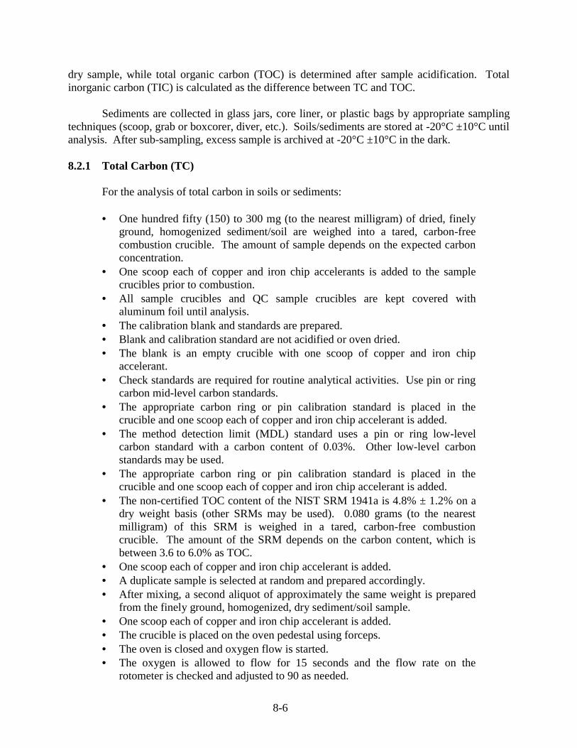
8-6

dry sample, while total organic carbon (TOC) is determined after sample acidification. Totalinorganic carbon (TIC) is calculated as the difference between TC and TOC.

Sediments are collected in glass jars, core liner, or plastic bags by appropriate samplingtechniques (scoop, grab or boxcorer, diver, etc.). Soils/sediments are stored at -20°C ±10°C untilanalysis. After sub-sampling, excess sample is archived at -20°C ±10°C in the dark.

8.2.1 Total Carbon (TC)

For the analysis of total carbon in soils or sediments:

• One hundred fifty (150) to 300 mg (to the nearest milligram) of dried, finelyground, homogenized sediment/soil are weighed into a tared, carbon-freecombustion crucible. The amount of sample depends on the expected carbonconcentration.

• One scoop each of copper and iron chip accelerants is added to the samplecrucibles prior to combustion.

• All sample crucibles and QC sample crucibles are kept covered withaluminum foil until analysis.

• The calibration blank and standards are prepared.• Blank and calibration standard are not acidified or oven dried.• The blank is an empty crucible with one scoop of copper and iron chip

accelerant.• Check standards are required for routine analytical activities. Use pin or ring

carbon mid-level carbon standards.• The appropriate carbon ring or pin calibration standard is placed in the

crucible and one scoop each of copper and iron chip accelerant is added.• The method detection limit (MDL) standard uses a pin or ring low-level

carbon standard with a carbon content of 0.03%. Other low-level carbonstandards may be used.

• The appropriate carbon ring or pin calibration standard is placed in thecrucible and one scoop each of copper and iron chip accelerant is added.

• The non-certified TOC content of the NIST SRM 1941a is 4.8% ± 1.2% on adry weight basis (other SRMs may be used). 0.080 grams (to the nearestmilligram) of this SRM is weighed in a tared, carbon-free combustioncrucible. The amount of the SRM depends on the carbon content, which isbetween 3.6 to 6.0% as TOC.

• One scoop each of copper and iron chip accelerant is added.• A duplicate sample is selected at random and prepared accordingly.• After mixing, a second aliquot of approximately the same weight is prepared

from the finely ground, homogenized, dry sediment/soil sample.• One scoop each of copper and iron chip accelerant is added.• The crucible is placed on the oven pedestal using forceps.• The oven is closed and oxygen flow is started.• The oxygen is allowed to flow for 15 seconds and the flow rate on the

rotometer is checked and adjusted to 90 as needed.

8-7

• After 15 seconds with the correct flow, the integrator is started and pedestallever is pushed in to start the induction furnace.

• Approximately 20 seconds after the furnace is activated, the carbon begins tocombust.

• About one minute after turning the furnace on, the ammeter will reach 500mA.

• When the signal returns to a baseline value, the furnace is turned off.• All calibration and sample analyses are recorded.

8.2.2 Total Organic Carbon (TOC)

For the analysis of soils and/or sediments for TOC:

• An appropriate amount of dried sample and duplicate sample is weighed andprepared in a tared crucible as described above.

• Small amounts of 10% HCl solution are slowly added to the sample until allbubbling stops. Use the smallest volume of acid possible.

• The treated samples are dried overnight at 50°C in a drying oven.• One scoop each of copper and iron chip accelerants is added to all of the

sample crucibles.• The above procedures are followed for combusting the TOC samples.• The calibration blank and standards are prepared in the same manner. The

laboratory blank is added to an empty crucible which has been acidified andplaced in the 50ºC oven overnight.

• One scoop each of copper and iron chip accelerant is added.• Check standards are standards with a mid-level carbon content. These

standards are not acidified.• The appropriate carbon ring or pin calibration standard is placed in the

crucible and one scoop each of copper and iron chip accelerant is added.• The method detection limit (MDL) standard uses a low-level carbon standard

between 0.03 and 0.07%. Other low-level carbon standards may be used.These standards are not acidified.

• The appropriate carbon calibration standard is placed in the crucible and onescoop each of copper and iron chip accelerant is added.

• The non-certified TOC content of the NIST SRM 1941a is 4.8 ± 1.2 % on adry weight basis.

• 0.080 grams (to the nearest milligram) of this SRM is weighed in a tared,carbon-free combustion crucible.

• The SRM is acidified and oven dried as described above. One scoop each ofcopper and iron chip accelerant is added.

• The duplicate sample is selected and prepared at random.• A second aliquot of approximately the same weight is prepared from the

finely ground, homogenized, dry sediment/soil sample.• The duplicate described above is acidified and oven dried.• One scoop each of copper and iron chip accelerant is added. The crucibles

used for these blanks are not acidified or oven dried.

8-8

• The calibration samples, the acidified samples, and associated QC samples areanalyzed as described above.

• All data regarding calibration activities and sample analyses are recorded.

8.2.3 Total Inorganic Carbon (TIC)

The % total inorganic carbon (TIC) content is determined by subtracting the % totalorganic carbon (TOC) from the % total carbon (%TC) content.

The following is an example analytical sequence.

Activity QC Criteria

Calibrate; blank plus four standards r2 �0.995

Check Standard (Mid-Level) ± 10% of true valueSRM 1941a ± 25% of true (3.6 -6.0% C)MDL standard (approx. 0.014-0.029% C) ± 25% of true value1. Prep. Blank �3xMDL2. Orig. Sample (�0.3 gram) Within Calibration Range3. Duplicate Sample (�0.3 g) RPD �25% Low % (<1%) %C

RPD �20% High %(>1%) C4. to 10. Samples (�0.3 g) Within Calibration RangeCheck Standard (Mid-Level) ± 15% of true value11. to 18. samples (�0.3 g) Within Calibration RangeCheck Standard (Mid-Level) ± 15% of true value

8.2.4 Calculations

Quality control samples are prepared and analyzed in an identical manner to the actualsamples. A five point initial calibration curve is prepared each day prior to analyzing samples.The QC acceptance criteria for the initial calibration curve is a correlation coefficient � 0.995.Analytical results determined by this procedure must be within the calibration range establishedfor the calibration curve. If not, sample size is reduced or the calibration range extended. Mid-level standards with carbon are analyzed after the calibration curve has been established. Checkstandards are also analyzed after every 10 samples (or with every sample set, whichever is morefrequent). A check standard is also analyzed at the end of the analytical sequence as a check.The QC acceptance criteria for the check standard is ± 15% of the known value. If the checkstandard fails this criteria, the analyses are stopped and the instrument recalibrated. A laboratoryblank is analyzed with every 20 samples, or with every sample set, whichever is more frequent.The QC acceptance criteria for carbon in the blank is less than or equal to three times thedetection limit (�0.06%). If this QC criteria is not met, all samples must be re-prepared and re-analyzed. Duplicate samples are analyzed every 20 samples, or with every sample set,whichever is more frequent. Except as noted below, the QC acceptance criteria for the RPD forduplicates is an RPD of ±25% for low level (<1.0% carbon) samples and �20% for high level(>1.0% carbon) samples. If this QC criteria is not met, all samples must be re-prepared and re-analyzed unless the samples are inhomogeneous. A higher RPD is acceptable forinhomogeneous samples (i.e., peat, sandy loams, grasses, shell hash, etc.). The non-certifiedTOC content of the NIST SRM 1941a is 4.8 ± 1.2 % on a dry weight basis (other SRMs may beused). This SRM is analyzed for every 20 samples and the QC acceptance criteria for the carboncontent of SRM 1941a is between 3.6 to 6.0 % TOC. This is equivalent to a percent recovery of

8-9

75 to 125% (± 25% of the known value). If an SRM fails the QC criterion, the instrument mustbe recalibrated, a check standard analyzed, and all samples are re-analyzed. A MDL standardcontaining between 0.03 and 0.07% carbon is analyzed with every 20 samples, or with everysample set, whichever is more frequent. Other low-level carbon standards may be used. The QCacceptance criteria for carbon levels in the MDL standard is ± 25% of the known value for thestandard used. If the MDL standard analysis fails the criterion, the instrument must berecalibrated, a check standard analyzed and all samples are re-analyzed.

Prior to sample combustion, a set of standards is analyzed to establish an initialcalibration curve. All data regarding calibration and sample analyses are recorded.

To determine the calibration curve, combust one blank and four carbon standards at %carbon contents of approximately 0.03, 0.390, 0.652, and 0.835%. Other carbon standards canbe used. The values of the standards in the set cover the 0 to 0.8% carbon calibration range(based on a sample weight of 1 gram). The calibration blank is an empty crucible containing onescoop each of copper and iron chip accelerators. The calibration blank is not acidified and iscombusted prior to the carbon standards. The appropriate carbon ring or pin calibrationstandards are placed in the crucible and one scoop each of copper and iron chip accelerators isadded prior to combustion. Calibration standards are not acidified.

A graphic representation of the calibration curve (integrator response vs. carbonpercentage) is used to calculate the best fit equation for the data. The QC acceptance criterionfor the calibration curve is that the correlation coefficient, r2, should be ��0.995. Calibrationanalyses are repeated until the QC criterion are met. The calibration curve is used to determinethe carbon content of the samples analyzed.

8.3 Metals

The methods for metals often provide for the determination of a large number of metalswith a single technique. Thus the metal methods are considered slightly different from the othermethods in this manual. Since the same metal can be determined by multiple instrumentaltechniques it is most effective to describe these methods by technique. In many cases themethods provide substantially different detection limits and the method of choice will depend onthe ambient levels expected in the matrix of interest. Certain methods, such as for mercury, havebeen specifically developed for the characteristics of the analyte of interest. Access to varioustypes of instruments may also be limited and therefore the selection of the method is at theanalyst’s discretion. For the specific metals of interest in this first tier of methods the followingmethods are recommended: cadmium (Cd) and lead (Pb) - graphite furnace atomic absorptionspectrophotometry (GFAAS), copper (Cu) and zinc (Zn) - inductively-coupled plasma emissionspectroscopy (ICP), and mercury (Hg) - cold vapor atomic absorption spectroscopy (CVAAS). Ineach instance the protocols for all other metals that can be analyzed by the various techniques arealso provided. As far as matrix, once the metals are converted to a soluble form, the instrumentalmethod is usually the same and may only need to take into account differences in concentrationsand/or interferences.

8-10


The choice of metals for a monitoring program are based on the potential sources in thearea and the known potential to induce biological effects. Metals are a common pollutantreleased by human activities and they can be derived from a wide range of sources. Metals arederived from the disposal of various types of materials (metal debris, batteries, etc.),degeneration of structures, construction activities (such as welding), and from metallic plumbingsystems. Metals are known to be toxic to biological organisms. However, the mere presence ofa chemical, in and of itself, does not indicate that adverse biological effects have occurred. Theavailability of the metal and its geochemical behavior will ultimately determine the potential forexposure and whether an adverse effect occurs in an exposed biological community. Differentorganisms also have differing sublethal and toxic response thresholds to metals. As a firstindication of the degree of contamination, establishment of the concentration and distribution ofmetals is important. The observed concentrations can be compared, at least qualitatively, todocumented effects levels in order to make a first assessment of the potential for biologicalimpacts. It should also be recognized that metals naturally occur in soils and sediments and thatanthropogenic inputs are in addition to these natural levels. It is important to establishbackground levels within a study area so that increases due to human activity can beunambiguously recognized.

The metals of interest for Antarctic monitoring programs were chosen based onknowledge of the expected outputs from typical activities that occur at stations and the availablemetal information previously collected and include cadmium, lead, copper, zinc, and mercury. Abrief description of suspected levels of biological effects is provided for each metal.

Studies have documented biological effects associated with cadmium levels of 5 mg/kgand higher (Long and Morgan 1990). Effects include mortality, reduced growth, inhibitedreproduction, and other adverse effects. Most studies were of freshwater and marineinvertebrates. Copper levels in sediments of 17.8 to 2820 mg/kg have been associated withbiological effects. Zinc concentrations in sediments of 50 to 250 mg/kg are associated withsublethal biological effects and effects almost always occurred at zinc concentrations above 260mg/kg. Biological effects have been observed for mercury sediment concentrations as low as0.15 mg/kg. It should be noted that these threshold levels for biological effects are only advisoryand actual metal concentrations in the field may or may not be reflective of these data.

8.3.1.1 Acid Digestion Procedure for ICP, Flame AA and Furnace AA Analyses

A representative 1 g (wet weight) sample is digested in nitric acid and hydrogenperoxide. The digestate is then refluxed with either nitric acid or hydrochloric acid.Hydrochloric acid is used as the final reflux acid for the furnace AA analysis of Sb, the FlameAA or ICP analysis of Al, Sb, Ba, Be, Ca, Cd, Cr, Co, Cu, Fe, Pb, Mg, Mn, Ni, K, Ag, Na, Tl, Vand Zn. Nitric acid is employed as the final reflux acid for the Furnace AA analysis of As, Be,Cd, Cr, Co, Cu, Fe, Pb, Mn, Ni, Se, Ag, Tl, V, and Zn.

The procedure is as follows:

• Mix the sample thoroughly to achieve homogeneity.

8-11

• For each digestion procedure, weigh (to the nearest 0.01g) a 1.0 to 1.5 gportion of sample and transfer to a beaker.

• Add 10 mL of 1:1 nitric acid (HNO3), mix the slurry, and cover with a watchglass. Heat the sample to 95oC and reflux for 10 minutes without boiling.

• Allow the sample to cool, add 5 mL of concentrated HNO3, replace the watchglass, and reflux for 30 minutes. Do not allow the volume to be reduced toless than 5 mL while maintaining a covering of solution over the bottom of thebeaker.

• After the second reflux step has been completed and the sample has cooled,add 2 mL of Type II water and 3 mL of 30% hydrogen peroxide (H2O2).

• Return the beaker to the hot plate for warming to start the peroxide reaction.Care must be taken to ensure that losses do not occur due to excessivelyvigorous effervescence. Heat until effervescence subsides, and cool thebeaker.

• Continue to add 30% H2O2 in 1 mL aliquots with warming until theeffervescence is minimal or until the general sample appearance is unchanged.[NOTE: Do not add more than a total of 10 mL 30% H2O2].

• If the sample is being prepared for the furnace AA analysis of Sb, the flameAA or ICP analysis of Al, Sb, Ba, Be, Ca, Cd, Cr, Co, Cu, Fe, Pb, Mg, Mn,Ni, K, Ag, Na, Tl, V, and Zn, add 5 mL of 1:1 HCl and 10 mL of Type IIwater, return the covered beaker to the hot plate, and heat for an additional 10minutes.

• After cooling, filter through Whatman No. 42 filter paper (or equivalent) anddilute to 100 mL with Type II water. [NOTE: In place of filtering, the sample(after dilution and mixing) may be centrifuged or allowed to settle by gravityovernight to remove insoluble material. The diluted sample has anapproximate acid concentration of 2.5% (v/v) HCl and 5% (v/v) HNO3.Dilute the digestate 1:1 (200 mL final volume) with acidified water tomaintain constant acid strength. The sample is now ready for analysis].

• If the sample is being prepared for the furnace analysis of As, Be, Cd, Cr, Co,Cu, Fe, Pb, Mn, Ni, Se, Ag, Tl, V, and Zn, continue heating the acid-peroxidedigestate until the volume has been reduced to approximately 2 mL, add 10mL of Type I water, and warm the mixture.

• After cooling, filter through Whatman No. 42 filter paper (or equivalent) anddilute the sample to 100 mL with Type I water (or centrifuge the sample).[NOTE: In place of filtering, the sample (after dilution and mixing) may becentrifuged or allowed to settle by gravity overnight to remove insolublematerial. The diluted digestate solution contains approximately 2% (v/v)HNO3. Dilute the digestate 1:1 (200 mL final volume) with acidified water tomaintain constant acid strength. For analysis, withdraw aliquots of appropriatevolume, and add any required reagent or matrix modifier. The sample is nowready for analysis.]

8-12

“Apparatus, Materials, and Reagents”

• 250 mL beaker or other appropriate vessel• Watch glasses• Thermometer that covers range of 0 to 200ºC• Whatman No. 42 filter paper or equivalent• ASTM Type II water (ASTM D1193): Water must be monitored• Concentrated nitric acid (sp. gr. 1.41)• Concentrated hydrochloric acid (sp. gr. 1.19)• Hydrogen Peroxide (30%)

8.3.1.2 Total Metals Sample Preparation Using Microwave Digestion

A representative 0.5 g (wet weight) sample is digested in 10 mL of concentrated nitricacid in a Teflon(R) PFA vessel or equivalent for 10 minutes using microwave heating. Thedigestate is then filtered to remove insoluble material. The sample may be centrifuged or allowedto settle by gravity overnight to remove insoluble material. [NOTE: This microwave digestionmethod is not appropriate for the quantitative recovery of Antimony from soil and sedimentsamples.]

The calibration procedure is a critical step prior to the use of any microwave unit. Themicrowave unit must be calibrated every six months. The calibration data for each calibrationmust be available for review during on-site audits. In order to interchange the absolute powersettings from one microwave unit to another, the actual delivered power must be determined.

Calibration of a laboratory microwave unit depends on the type of electronic system usedby the manufacturer. If the unit has a precise and accurate linear relationship between the outputpower and the scale used in controlling the microwave unit, then the calibration can be a two-point calibration at maximum and 40% power. If the unit is not accurate or precise for someportion of the controlling scale, then a multiple-point calibration is necessary. If the unit powercalibration needs a multiple-point calibration, then the point where linearity begins must beidentified. For example: a calibration at 100, 99, 98, 97, 95, 90, 80, 70, 60, 50 and 40% powersettings can be applied and the data plotted. The non-linear portion of the calibration curve canbe excluded or restricted in use. Each percent is equivalent to approximately 5.5-6 watts andbecomes the smallest unit of power that can be controlled. If 20-40 watts are contained from 99-100%, that portion of the microwave calibration is not controllable by 3-7 times that of the linearportion of the control scale and will prevent duplication of precise power conditions specified inthat portion of the power scale.

The power available for heating is evaluated so that the absolute power setting (watts)may be compared from one microwave to another. This is accomplished by measuring thetemperature rise in 1 Kg of water exposed to microwave radiation for a fixed period of time. Thewater is placed in a Teflon(R) beaker (or a beaker that is made of some other material that doesnot adsorb microwave energy) and stirred before measuring the temperature. Glass beakersadsorb microwave energy and may not be used. The initial temperature of the water must bebetween 19 and 25ºC. The beaker is circulated continuously through the field for at least two (2)minutes at full power. The beaker is removed from the microwave, the water is stirred

8-13

vigorously, and the final temperature recorded. The final reading is the maximum temperaturereading after each energy exposure. These measurements must be accurate to ±0.1ºC and madewithin 30 seconds of the end of heating. If more measurements are needed, do not use the samewater until it has cooled down to room temperature. Otherwise, use a fresh water sample.

The absorbed power is determined by the following formula:

P = [(K) x (Cp) x (m) x (DT)] / t

where:

P = The apparent power absorbed by the sample in watts (joules per second),K = The conversion factor for thermochemical calories per second to watts (-4.184),Cp = The heat capacity, thermal capacity, or specific heat (cal. g-1ºC-1) of water (-1.0),m = The mass of the sample in grams (g),DT = the final temperature minus the initial temperature (ºC), andt = the time in seconds (s)

Using 2 minutes and 1 Kg of distilled water, the calibration equation simplifies to:

P = (DT) (34.87).

The microwave user can now relate power in watts to the percent power setting of the microwave

The initial cleaning of the PFA vessels:

• Prior to first use - new vessels must be annealed before they are used. Apretreatment/cleaning procedure must be followed. This procedure calls forheating the vessels for 96 hours at 200ºC. The vessels must be disassembledduring annealing and the sealing surfaces (the top of the vessel or its rim)must not be used to support the vessel during annealing.

• Rinse in ASTM Type I water.• Immerse in 1:1 HCl for a minimum of 3 hours after the cleaning bath has

reached a temperature just below boiling.• Rinse in ASTM Type I water.• Immerse in 1:1 HNO3 for a minimum of 3 hours after the cleaning bath has

reached a temperature just below boiling.• The vessels are then rinsed with copious amounts of ASTM Type I water prior

to use for any analyses under this contract.

Cleaning procedure between sample digestions

• Wash entire vessel in hot water using laboratory-grade nonphosphatedetergent.

• Rinse with 1:1 nitric acid.

8-14

• Rinse three times with ASTM Type I water. If contaminants are found in thepreparation blank, it is mandatory that steps a(2) through a(6) be strictlyadhered to.

The digestion procedure is as follows:

• Add a representative 0.5 ±0.050 grams of sample to the Teflon(R) PFA vesselor equivalent.

• Add 10 ±0.1 mL of concentrated nitric acid. If a vigorous reaction occurs,allow the reaction to stop before capping the vessel.

• Cap the vessel, then tighten using constant torque to 12 ft/lbs, according to themanufacturer's direction.

• Connect the sample vessel to the overflow vessel using Teflon(R) PFA tubingor equivalent.

• Weigh the vessel assembly to the nearest 0.01g.• Place sample vessels in groups of 2 sample vessels or 6 sample vessels in the

carousel, evenly spaced around its periphery in the microwave unit. If fewerthan the recommended number of samples are to be digested (i.e., 3 samplesplus 1 blank) then the remaining vessels must be filled with 10 mL of nitricacid to achieve the full complement of vessels. Each sample vessel must beattached to a clean, double-ported vessel to collect any sample expelled fromthe sample vessel in the event of over pressurization. Assembly of the vesselsinto the carousel may be done inside or outside the microwave. Connect theoverflow vessel to the center well of the oven.

• The preparation blank must have 0.5 mL of deionized water and the sameamount (10 mL) of acid that is added to the samples. The preparation blankmust later be diluted to 50 mL in the same manner as the samples.

• Irradiate the 2 sample vessel group at 344 watts for 10 minutes, or the 6sample vessel group at 574 watts for 10 minutes. This program brings thesamples to 175ºC in 5.5 minutes; the temperature remains between 170-180ºCfor the balance of the 10 minute irradiation period. The pressure should peakat less than 6 atm for most samples. The pressure may exceed these limits inthe case of high concentrations of carbonate or organic compounds. In thesecases, the pressure will be limited by the relief pressure of the vessel to 7.5±0.7 atm.

• Allow the vessels to cool for a minimum of five minutes before removingthem from the microwave unit, with exhaust fan on. Allow the vessels to coolto room temperature before opening. The vessels must be carefully vented anduncapped in a fume hood.

• Weigh each vessel assembly. If the weight of acid plus the sample hasdecreased by more than 10% from the original weight, discard the digests.Determine the reason for the loss. Losses typically are attributed to use ofdigestion time longer than ten minutes, using too large of a sample, or havingimproper heating conditions. Once the source of the losses has been corrected,prepare a new set of samples for digestion.

• Sample Filtration: Shake the sample well to mix in any condensate within thedigestion vessel before being opened. Filter the digestion vessel into a 50 mL

8-15

glass volumetric flask through ultra-clean filter paper. Rinse the sampledigestion vessel, cap, connecting tube, and (if venting occurred) the overflowvessel into the 50 mL glass flask. Dilute to 50 mL. The samples are now readyfor analysis. Concentrations are reported as “total.”

“Apparatus, Materials, and Reagents”

Note: Commercial kitchen or home-use microwave ovens shall not be used for thedigestion of samples. The oven cavity must be corrosion resistant and well ventilated.All electronics must be protected against corrosion for safeoperation.• Microwave oven with programmable power settings up to atleast 600 Watts.• The system must use PFA Teflon(R) digestion vessels (120 mL capacity) capable

of withstanding pressures of up to 110 ±10 psi (7.5 ± 0.7 atm). These vessels arecapable of controlled pressure relief at pressures exceeding 110 psi.

• A rotating turntable must be used to ensure homogeneous distribution ofmicrowave radiation within the oven. The speed of the turntable must be aminimum of 3 rpm.

• Polymeric volumetric labware in plastic (Teflon(R) or polyethylene) 50 mL or100 mL capacity.

• Whatman No. 41 filter paper (or equivalent).• Disposable polypropylene filter funnel.• Analytical balance: 300 g capacity, and minimum ± 0.01 g.• Polyethylene bottles: 125 mL, with caps.• ASTM Type I water (ASTM D1193): water must be monitored.• Sub-boiled, concentrated nitric acid (sp. gr. 1.41).• Concentrated hydrochloric acid (sp. gr. 1.19).

8.3.1.3 Total Digestion of Sediment with Hydrofluoric Acid for Trace MetalAnalyses

A method is described herein for the preparation of bottom sediment samples for tracemetal analysis by atomic absorption spectrophotometry (AAS). Before samples can be analyzedby AAS methods in use in this laboratory, they must be converted from solid to liquid form.

• Wet sediment is homogenized in its container, and an aliquot is freeze driedand homogenized to a fine powder.

• Approximately 0.20 to 0.25 g of powdered sediment is weighed into a Teflonreaction vessel, 3 mL of concentrated HNO3 are added and the lid istightened.

• The vessel is heated in a 130°C oven for 24 hrs.• Concentrated hydrofluoric acid (2 mL) is added, the lid tightened, and the

reaction vessel is heated again for 24 hrs. at 130ºC.• Samples are then diluted to a final volume of 20 mL with 5% boric acid and

transferred to a polyethylene bottles for storage until analysis.

8-16


• Mortar and Pestle: To homogenize sample.• Reaction Vessels: Savillex 50 mL Teflon reaction vessels or equivalent.• Oven: Heated to 130°-135°C.• Disposable Plastic Transfer Pipets: 1 mL.• Balance: Top loading with accuracy of 0.01 g.• Analytical Balance: With an accuracy of 0.0001 g.• Screw Top Bottles: Nalgene or equivalent.• Reagent Water: Reagent water contains no analytes above the method detection

limit. Reagent water is produced by subboiling redistillation of water in a quartzstill.

• Concentrated Nitric Acid: Baker Ultrex Grade or equivalent, stored in Teflonbottle.

• Concentrated Hydrofluoric Acid: Baker analyzed or equivalent.• Boric Acid: Ultrex grade or equivalent.

8.3.2 Graphite Furnace Atomic Absorption Spectrophotometry (GFAAS)

Graphite furnace atomic absorption spectrophotometry (GFAAS) relies on the electricalresistance heating generated by passing an electrical current through a graphite tube to evaporatethe solvent (water), remove interfering species, and finally atomize the analyte into the light pathof an absorption spectrophotometer. This technique is approximately two orders of magnitudemore sensitive than Flame AAS (FAAS), primarily because the whole sample that is injectedinto the graphite tube is analyzed (as opposed to 10% in the case of FAAS), and because theabsence of a flame results in a better signal-to-noise ratio. However, the GFAAS technique ismuch slower, requiring up to several minutes for individual analyses and is generally much moresusceptible to interferences. GFAAS is recommended for cadmium (Cd) and lead (Pb)determinations.

“Apparatus, Materials, and Reagents - Cadmium and Lead”

• GFAAS: One example of a GFAAS instrument is a Perkin Elmer Zeeman 3030equipped with a HGA 600 furnace capable of an almost infinite range oftemperatures, heating rates and holding times.

• Autosampler: The GFAAS is equipped with an autosampler having 40 samplepositions and allows for delivery of sample and matrix modifier volumes from 1-99µL.

• Hollow cathode lamps: The use of special light sources and careful wavelengthselection permits the specific determination of one element in the presence ofothers. Hollow cathode lamps consist of a sealed glass cylinder filled with an inertgas, an anode, a cathode, and an end window. The cathode is a hollow cylinder ofthe element whose spectrum is to be produced.

• Electrodeless discharge lamps: Electrodeless discharge lamps (EDL) aretypically more intense and usually provide better sensitivity than hollow cathodelamps. EDLs consist of the element of interest or a salt sealed in a quartz bulbcontaining an inert atmosphere. The bulb is contained in a ceramic holder onwhich an radio frequency coil is wound.

• Balance: Top loading with accuracy of 0.01 g.

8-17

• Autosampler cups: 2.0 mL polystyrene autosampler cups.• Microliter pipettes: 1000-, 500-, 300-, 200-, 100-, 50-, 25- and 10-µL capacity.• Reagent water: Reagent water contains no analytes above the method detection

limit. Reagent water is produced by redistilling water in a quartz still.• Nitric acid: Baker Ultrex Grade or equivalent, stored in Teflon bottle.• Calibration standards: The calibration standards are prepared daily from

commercially available reference standards, diluted with reagent water, and matrix-matched to the acid content of the samples. The calibration blank consists ofreagent water, matrix-matched to the acid content of the samples. The higheststandard’s concentration is chosen to be at the upper end of either the expectedsample levels or the element's linear detection range, whichever is less. Eachelement has appropriate calibration standard concentrations and standard operatingconditions.

• Matrix recovery spiking solution: The volume and concentration of matrixspiking solution are element and sample dependent. In all cases, the goal is toincrease the observed concentration by 50%, while not diluting the sample matrixby more than 25%. When matrix spiking results in a concentration outside thecalibration range, the sample is diluted and reanalyzed.

• Matrix modifiers: The technique of GFAAS has been greatly advanced by the useof several matrix modifiers which remove or greatly diminish interferences fromsample matrix. The modifiers assist in the analysis by either increasing thevolatility of an interferent, or by increasing the analyte's thermal stability so thatthe sample may be charred at a higher temperature. Modifiers used for thispurpose are described below.

Instrumental operating conditions, matrix modifiers, and expected sensitivities are asfollows:

Element Source Wavelength Slit Site Matrix Modifier Char. Mass

Ag HCL 328.1 0.7 P 0.015 mg Pd + 1.50.01 mg Mg(NO3)2

As EDL 193.7 0.7 P 0.015 mg Pd + 15.0.01 mg Mg(NO3)2

197 0.7 P 0.015 mg Pd + 30.0.01 mg Mg(NO3)2

Cd EDL 228.8 0.7 P 0.2 mg PO4 + 0.350.01 mg Mg(NO3)2

Cr HCL 357.9 0.7 P 0.05 mg Mg(NO3)2 3.3Cu HCL 324.7 0.7 P 0.015 mg Pd + 8.0

0.01 mg Mg(NO3)2Fe HCL 248.3 0.2 P 0.05 mg Mg(NO3)2 5.0Mn HCL 279.5 0.2 P 0.05 mg Mg(NO3)2 2.2Mo HCL 313.3 0.7 W 9.0Ni HCL 232.0 0.2 P 13.0Pb EDL 283.3 0.7 P 0.2 mg PO4 + 12.0

0.01 mg Mg(NO3)2Sb EDL 217.6 0.7 P 0.015 mg Pd + 22.0

0.01 mg Mg(NO3)2Se EDL 196.0 0.7 P 0.015 mg Pd + 28.0

0.01 mg Mg(NO3)2

8-18

(Cont.)

Element Source Wavelength Slit Site Matrix Modifier Char. Mass

Sn EDL 286.3 0.7 P 0.015 mg Pd + 24.00.01 mg Mg(NO3)2

V HCL 318.4 0.7 W 0.05 mg Mg(NO3)2 40.0Zn HCL 213.9 0.7 P 0.006 mg Mg(NO3)2 0.45

where HCL = hollow cathode lamp,EDL = electrodeless discharge lamp,Wavelength and slit width are in nm,Site, “P” and “W” refer to “platform” and “wall” as the site of sample deposition, respectively,Characteristic mass is the mass of the analyte, in picograms, expected to result in a peak area of 0.0044 Abs-sec.

Calibration Standards for Graphite Furnace Concentration (ng/mL)

Element Calib. Blk. Low Std. Mid Std. High Std.

Ag 0 1.5 3.0 4.5As 0 20 40 60Cd 0 0.4 0.8 1.2Cr 0 4.0 8.0 12.0Cu 0 10 20 30Fe 0 5 10 15Mn 0 2.5 5.0 7.5Mo 0 10 20 30Ni 0 15 30 45Pb 0 15 30 45Sb 0 45 90 135Se 0 35 70 105Sn 0 25 50 75V 0 45 90 135Zn 0 0.1 0.2 0.3

An example analytical sequence:

Sequence Number Autosampler Position Contents

1 1 Cal. Blk.2 2 Low Std.3 3 Mid Std.4 4 High Std.5 5 Calibration Verification Spl. (CV)6 6 Sample7 7 Matrix Spike (MS) into Sample 68 8 Sample9 9 Sample10 10 Sample11 11 Sample12 12 Sample13 13 Sample14 14 Sample15 15 Sample16 16 Sample17 1 Cal. Blk.

8-19

(Cont.)

Sequence Number Autosampler Position Contents

18 2 Low Std.19 3 Mid Std.20 4 High Std.21 17 Sample22 18 Sample23 19 Sample24 20 Sample25 21 Sample26 22 Sample27 23 Sample28 24 Sample29 25 Sample30 26 Sample31 27 Sample32 28 Sample33 1 Cal. Blk.34 2 Low Std.35 3 Mid Std.36 4 High Std.37 29 CV38 30 Sample39 31 MS into sample in pos’n 3040 32 Sample41 33 Sample42 34 Sample43 35 Sample44 36 Sample45 37 Sample46 38 Sample47 39 Sample48 40 Dup. anal of spl from pos’n 649 1 Cal. Blk.50 2 Low Std.51 3 Mid Std.52 4 High Std.

Matrix spikes in this listing refer to post-digestion spikes.

Sample concentrations are determined from the calibration results and from the dilutionfactors involved in instrumental analysis and sample digestion according to the followingequation:

1000DFx]ConcDFxConc[)g/g(ionConcentrat n’dgPBsplspl ÷−=µwhere:

Concspl = the concentration observed in the sample, in µg/g,ConcPB = the concentration observed in the procedural blanks, in µg/g,DFspl = the dilution factor required to dilute the sample concentration to the working

range of the machine,DFdig'n = the dilution factor resulting from sample digestion, in mL/g.

8-20

Reporting units are µg/g dry or weight depending on protocol requirements. Theminimum method performance standard is dependent on the dilution factor resulting fromdigestion of sediment or soil sample and on the sensitivity of the technique for each element.General requirements for acceptable performance include instrumental sensitivity that is no lessthan 80% of that reported by the manufacturer or from historical records (instrumentalcharacteristic masses listed above). Results are reported to the number of significant figures thatmatches the number of such figures in the absorption reading. Samples with absorption less than0.010 are reported with only 1 significant figure, samples with absorption equal to or greater than0.010 and less than 0.100 have two significant figures, and samples with absorption greater thanor equal to 0.100 are reported with three significant figures.

Quality control samples are processed in a manner identical to actual samples. Onemethod blank is analyzed with every 20 samples or with every sample set, whichever is morefrequent. Blank levels should be no more than twice the method detection limit (MDL). If blanklevels are > 2x MDL, the analysis is repeated and the data reported if QC criteria are met. Ifblank results are still > 2x MDL, the sample set is reprocessed after the source of contaminationis isolated. If insufficient sample is available, data are reported with a blank correction and notedas such in the data.

One reference material is analyzed with every 20 samples or with every sample set.Sediment or water certified reference materials, if available, and as closely matching the sampleset as possible, are analyzed with each sample set. Reference materials include:

Sediment samples:BCSS-1 (NRCC, Canada),MESS-2 (NRCC, Canada), andEstuarine sediment, #1646 (NIST, U.S.),.

Water samples:CASS-2 (NRCC, Canada), andSLRS-1 (NRCC, Canada).

Reference material is deemed acceptable if the results are within 20% of the certifiedvalue (if this value is � 2x MDL) or within the 95% confidence interval, whichever is greater.

One matrix spike is analyzed with every 20 samples or with every sample set. Matrixspikes are used to investigate possible interferences which may result in either signalenhancement or suppression. Spiked and unspiked sample concentrations are compared andspike recovery is calculated according to the equation:

100x

V

VxC

CC(%)RecoverySpike

splspkd

spkspk

splsplspkd −=

where:

8-21

Cspkd spl = the concentration observed in the spiked sample,Cspl = the concentration observed in the unspiked sample,Cspk = the concentration of the spiking solution,Vspk = the volume of the spike solution used in making the spiked sample,Vspkd spl = the volume of the spiked sample = Vspl + Vspk

Spikes are deemed valid only if the analyte concentration of the sample is < 2x MDL andthe spiked concentration is doubled or increased by ≥ 4x the MDL, whichever is greater. Onlyvalid spikes can be judged acceptable or unacceptable. When spike concentration is less than10% of the sample concentration, calculations for matrix spikes are not performed.

One post-digestion matrix spike is analyzed with every 20 samples or with every sampleset. These spikes are used to investigate possible interferences which may result in either signalenhancement or suppression. A small volume of a standard is added to a portion of the sample,which is then analyzed. Spiked and unspiked sample concentrations are compared and spikerecovery is calculated according to the equation:

100xVC

VCVC(%)RecoverySpike

spkspk

splsplsplspkdsplspkd −=

where:

Cspkd spl = the concentration observed in the spiked sample,Vspkd spl = the volume of the spiked sample = Vspl + Vspk,Cspl = the concentration observed in the unspiked sample,Vspl = the volume of sample used in making the spiked sample,Cspk = the concentration of the spiking solution, andVspk = the volume of spike solution used in making the spiked sample.

Spikes are deemed valid only if the analyte concentration is < 2x MDL and the spikedsample concentration is doubled or increased by ≥ 4x the MDL, whichever is greater. Onlyvalid spikes can be judged acceptable or unacceptable.

One duplicate sample is analyzed with every 20 samples or with every sample set.Inhomogeneous samples may result in greater variability between duplicates. Experience hasindicated that reference materials are more homogeneous than are samples, and thus comparisonof the RPD of duplicates for a) reference material duplicate analyses, b) sample duplicateanalyses and c) duplicate analyses from single digestion solutions gives an indication of a) totalanalytical variability (i.e., processing + instrumental variability), b) the sum of analyticalvariability and natural sample inhomogeneity, and c) instrumental variability. For standard QApurposes, “duplicate analysis” consists of preparation and analysis of duplicate sample aliquots.An RPD of ± 20% is deemed acceptable for valid sample duplicate analyses (i.e., having analyteconcentrations ≥5x MDL or other values as required).

8-22

Two blank spikes are analyzed with every 40 samples or with every sample set. Blankspikes are method blanks that have been fortified and carried through the digestion and analyticalprocedures. Blank spikes are analyzed to identify any digestion interferences or losses, and toevaluate the performance of the analysis. Blank spike recovery is acceptable when it is within80-120% of the known value. If the recovery is outside these limits, the analysis is repeated andthe re-analysis data is reported if it meets the criterion. If more than 10% of the blank spikes in adelivery set are deemed unacceptable then samples corresponding to these analytical batches areredigested.

8.3.3 Inductively Coupled Plasma Emission Spectroscopy (ICP)

The following procedures are used for the analysis of trace metals using InductivelyCoupled Plasma (ICP) Emission Spectroscopy. The ICP techniques use a Leeman Labs PS-3000UV Inductively Coupled Plasma Spectrometer with Echelle grating optics and asequential/simultaneous combination detection system or equivalent instrumentation. Thismethod is recommended for copper (Cu) and zinc (Zn) determinations.

These instrumental procedures can be used for the analysis of trace metals in digestatesresulting from preparation of water, snow and sediment samples. The routine trace metalsquantitatively determined by this method, with their suggested wavelengths, are provided inTable 8.1. The following analytes can be determined semi-quantitatively using the proceduresdescribed in EPA Method 1620: Bi, Ce, Dy, Er, Eu, Gd, Ga, Ho, In, La, Lu, Nd, P, Sm, Sc, Sr,Tb, Tm, U, Yb, Ge, Au, Hf, Ir, Li, Nb, Pd, Pt, K, Rh, Re, Ru, Si, Ta, Te, Th, Zr, W, Os, Pr, andS.

Because it is difficult to find a “clean” matrix free of trace metals, instrument detectionlimits (IDLs) are routinely used for ICP analyses instead of method detection limits. The IDL isestablished by performing seven consecutive measurements using a standard solution at aconcentration three to five times the estimated IDL. These measurements are performed on threenon-consecutive days and the resulting average standard deviation is multiplied by three todetermine the IDL. If multiple instruments are used, an IDL is determined for each instrument.The IDL is determined quarterly and the highest IDL is used during that quarter for reporting alldata from all ICPs. The IDL represents the minimum concentration of an element that can bemeasured and reported with 99% confidence that the element concentration is greater than zero.

The method detection limit (MDL) is defined as the minimum concentration of an analytethat can be measured and reported with 99% confidence that the analyte concentration is greaterthan zero. MDLs are determined by the preparation, digestion, and analysis of a “clean” samplematrix, either spiked with or containing the target analytes, following the procedures required by40 CFR, Part 160, Appendix B. The composition of the routine analytical standards used forinstrument calibration are provided in Tables 8.2 and 8.3. Calibrations are linear over the rangeof the standards used. Quarterly linear range studies prove that the linearity of the instrumentaldeterminations extends beyond the highest calibration standards for most elements. Whensample concentrations exceed the linear range, the sample is diluted and re-analyzed. There areno significant spectral overlaps found for the wavelengths listed in Table 8.1. An inter-elementcorrection factor study is performed annually. As a result, no significant interelement correctionfactors have been found to be necessary. Background correction points are used to compensate

8-23

Table 8.1. Wavelength Used for Routine ICP Quantitative Trace Metal Analytes.

Element Wavelength (nm)

Aluminum Al 308.215Antimony Sb 206.833Arsenic As 193.695Barium Ba 455.403

Beryllium Be 234.861Boron B 249.678

Cadmium Cd 214.438Calcium Ca 317.933

Chromium Cr 267.716Cobalt Co 228.616Copper Cu 324.754

Iron Fe 259.940Lead Pb 220.353

Magnesium Mg 279.079Manganese Mn 257.610

Molybdenum Mo 202.030Nickel Ni 231.604

Potassium K 766.490Selenium Se 196.026

Silver Ag 328.068Sodium Na 589.592

Strontium Sr 421.552Tin Sn 189.946

Titanium Ti 334.941Vanadium V 310.230Yttrium Y 371.030

Zinc Zn 206.200

for matrix related spectral interferences. The analyst has the responsibility for applyingbackground correction depending on the particular wavelength, matrix, concentration range andcalibration equation applied. Background correction is required for the weighted linearcalibration used by this ICP’s software. Physical interferences associated with samplenebulization and transport processes may be observed when samples with high amounts of totaldissolved material are analyzed. The use of a peristaltic pump significantly lessens theseinterferences. However, samples with high dissolved solids may require dilution prior toanalysis. If the estimated amount of total dissolved material in a diluted sample is higher than1000 ppm, the matrix matching techniques should be used. Method specific quality control(QC) acceptance criteria are summarized in Table 8.4.

A peaking routine should be performed after the instrument has warmed up at least 30minutes and prior to sample analysis. “Peaking” on the X and Y axes locates the best viewingposition in the plasma and checks nebulizer argon pressure. Peaking should be performed usinga manganese solution of 20-100 ppm. Peaks should be centered and even. If the Y peak isuneven or erratic, the nebulizer may need to be adjusted or a leak may have been detected.

8-24

Table 8.2. Calibration Standard Concentration.

Standard Identifier Analytes and their concentrations (µg/mL) Matrix

(Also used as CCB) Ca, Na, K 200 10% Nitric AcidS4* ScanM Al, Ca, Fe, Mg, Na, K 100

Ba, Sb 10Be, Cd, Co, Cu, Mn 5Ni, V, Zn 5

5% Nitric Acid

S3* ScanM (Alsoused as ICV)

Al, Ca, Fe, Mg, Na, K 20Ba, Sb 1Be, Cd, Co, Cu, Mn 0.5Ni, V, Zn 0.5

5% Nitric Acid

S2* ScanM Al, Ca, Fe, Mg, Na, K 4Ba, Sb 0.1Be, Cd, Co, Cu, Mn 0.05Ni, V, Zn 0.05

5% Nitric Acid

S1* ScanM/Q(Also used as CCB)

5% Nitric Acid

S4* ScanQ As, Pb, Se 10B, Mo, Sr, Cr 5

5% Nitric Acid

S3* ScanQ (Alsoused as ICV)

As, Pb, Se 1B, Mo, Sr, Cr 0.5

5% Nitric Acid

S2* ScanQ As, Pb, Se 0.1B, Mo, Sr, Cr 0.05

5% Nitric Acid

*Standards are used for sediment calibration standards.

Consult the ICP manual to correct the problem. Prior to sample analysis, a daily instrument QCtest is performed to ensure that the instrument, particularly the sample introduction components,are operating correctly. Performance is determined by evaluating the reproducibility of a dailyQC solution which has been analyzed twenty consecutive times. The relative standard deviation(RSD) calculated by the instrument software for each analyte should be <1%. If the RSDexceeds the QC acceptance criterion, corrective action is taken. The daily QC data is stored inthe file for daily QC runs.

A 4-point calibration curve, using background correction, is used in this procedure. TheICP is linear over a wide concentration range. The ICP software uses a weighted linear least-square fit for low-level determinations which permits low concentrations to have more of animpact on the fit of calibration line. The correlation coefficient should be ≥0.9950 for eachanalyte in the calibration curve. The absolute value of the concentration for an element in thecalibration blank should be less than the ML for each element in question. The RSD for threereplicates at 10 ppm level should be ≤1% and at 1 ppm the RSD should be ≤5% for mostelements. Significantly worse precision may be due to inadequate uptake time, exhausting thestandard, sample introduction problems, solution chemistry, or wavelength alignment. Theinitial calibration is stored in the appropriate ICP calibration file.

A matrix matched blank (CCB; Table 8.2) is analyzed after each calibration and/or at thebeginning of each analytical set. If the absolute calculated value for any analyte is higher thanthe ML, corrective action is taken. Corrective action may include a calibration update,instrumental maintenance and/or recalibration. A matrix matched blank (CCB; Table 8.2) isanalyzed after each 10 samples or after each 2 hour period (whichever is sooner) and at the

8-25

completion of each analytical set. If the absolute calculated value for any analyte is higher thanthe ML, corrective action is taken. Corrective action may include terminating analysis, acalibration update, instrument maintenance and/or recalibration. A matrix matched low (ICV,Table 8.2) or mid-level standard (CCV, Table 8.3) is analyzed after calibration and/or at thebeginning of each set. The QC acceptance criteria required for each analyte is a concentrationdetermination of 90 to 110% of the true value. If any analyte value is outside of the acceptancecriteria, corrective action is taken, which may include a calibration update, instrumentmaintenance and/or recalibration. A matrix matched mid-level standard (CCV, Table 8.3) isanalyzed after each 10 samples or after each 2 hour period (whichever is sooner) and at thecompletion of each analytical set. The QC acceptance criteria required for each analyte is aconcentration determination of 90 to 110% of the true value. If any analyte value is outside ofthe QC acceptance criteria, corrective action is taken, which may include terminating analysis, acalibration update, instrumental maintenance and/or recalibration.

As a result of changes in the laboratory environment, the light intensities measured for agiven concentration may change slightly. A corrective “calibration update” procedure can beused to adjust the calibration line. There are two update options, the intercept update and theslope update, which are described in the following sections. The intercept update should alwaysbe performed first, especially if problems are indicated with the calibration blank (ICB/CCB)standard. The slope update follows the intercept update, if needed, when there are problems withthe low or mid-level check standard (CK2, ICV or CCV). The “Intercept update” determines anadditive correction factor and is calculated after analyzing a single intercept update standard(standard 1; S1; Table 8.2) in this procedure. The QC acceptance criteria requires that theintercept correction for each analyte should be <2 times the CRDL or ML or recalibration shouldbe performed. The “slope update” determines a multiplicative correction factor to the calibrationequation and is calculated after the intercept update by analyzing a single slope update standardcontaining all elements (standard 4; S4; Table 8.2) in this procedure. The QC acceptance criteriarequires that the % slope correction for each analyte included in the slope update should be<10% or recalibration procedures should be performed. The continuing calibration blank (CCB)and continuing calibration verification (CCV) standards are used to validate the calibrationupdate(s).

All data from QC samples are evaluated for a specific digestion batch and analyticalsequence before making decisions regarding corrective actions. However, contamination of themethod blank normally requires complete analysis of the batch, unless the analyte concentrationin all samples is 10 times that in the blank. A method blank is used to demonstrate that samplepreparation, digestion, and analytical procedures are free of contamination. A method blank isrequired for each set of 20 or fewer samples in a preparation/digestion batch. The QCacceptance criteria for the method blank specifies that if the target analytes are present inconcentrations >2 times the ML, the preparation/digestion batch requires re-digestion, unless theconcentration in a sample is 10 times that found in the method blank. Analyst discretion is usedwhen contamination is present which does not adversely affect the overall analysis.

A sample duplicate (DUP) is used to evaluate matrix homogeneity and analyticalprecision in the presence of a representative matrix and is required with each set of 20 or fewersamples. The QC acceptance criteria for duplicate analyses is that the relative percent difference(RPD) between the original and its duplicate should not exceed 20%. The DUP QC acceptance

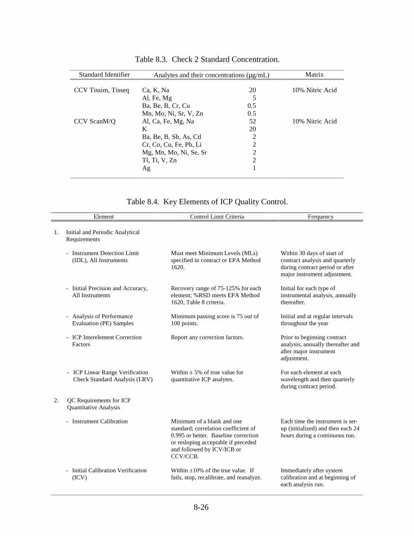
8-26

Table 8.3. Check 2 Standard Concentration.

Standard Identifier Analytes and their concentrations (µg/mL) Matrix

CCV Tissim, Tisseq Ca, K, Na 20Al, Fe, Mg 5Ba, Be, B, Cr, Cu 0.5Mn, Mo, Ni, Sr, V, Zn 0.5

10% Nitric Acid

CCV ScanM/Q Al, Ca, Fe, Mg, Na 52K 20Ba, Be, B, Sb, As, Cd 2Cr, Co, Cu, Fe, Pb, Li 2Mg, Mn, Mo, Ni, Se, Sr 2Tl, Ti, V, Zn 2Ag 1

10% Nitric Acid

Table 8.4. Key Elements of ICP Quality Control.

Element Control Limit Criteria Frequency

1. Initial and Periodic AnalyticalRequirements

- Instrument Detection Limit(IDL), All Instruments

Must meet Minimum Levels (MLs)specified in contract or EPA Method1620.

Within 30 days of start ofcontract analysis and quarterlyduring contract period or aftermajor instrument adjustment.

- Initial Precision and Accuracy,All Instruments

Recovery range of 75-125% for eachelement; %RSD meets EPA Method1620, Table 8 criteria.

Initial for each type ofinstrumental analysis, annuallythereafter.

- Analysis of PerformanceEvaluation (PE) Samples

Minimum passing score is 75 out of100 points.

Initial and at regular intervalsthroughout the year

- ICP Interelement CorrectionFactors

Report any correction factors. Prior to beginning contractanalysis, annually thereafter andafter major instrumentadjustment.

- ICP Linear Range VerificationCheck Standard Analysis (LRV)

Within ± 5% of true value forquantitative ICP analytes.

For each element at eachwavelength and then quarterlyduring contract period.

2. QC Requirements for ICPQuantitative Analysis

- Instrument Calibration Minimum of a blank and onestandard; correlation coefficient of0.995 or better. Baseline correctionor resloping acceptable if precededand followed by ICV/ICB orCCV/CCB.

Each time the instrument is set-up (initialized) and then each 24hours during a continuous run.

- Initial Calibration Verification(ICV)

Within ±10% of the true value. Iffails, stop, recalibrate, and reanalyze.

Immediately after systemcalibration and at beginning ofeach analysis run.

8-27

Table 8.4. (Cont.)


- Initial Calibration Blank (ICB) Absolute value �ML for quantitativeanalyses. When fails, recalibrate,reprocess with ICV, ICB.

After every ICV.

- ICP Minimum Level StandardSolution

Use ICP standard at 2x ML or 2xIDL, whichever is greater. Compareto MLs on Table 3.2; control limitsnot yet specified; report recoveries.

After ICV/ICB and at end ofeach analysis run or twice per 8-hour shift, whichever is morefrequent. CCV, CCB mustfollow analysis of the sample.

- Continuing CalibrationVerification (CCV)

Within ±10% of the true value. Iffails, stop, recalibrate, and reanalyzeback to last passing CV. Same CCVmust be used for entire Episode orsample set.

At a minimum of every 10% orevery 2 hours during an analysisrun, and after the last analyticalor QC sample.

- Continuing Calibration Blank(CCB)

Absolute value �ML for quantitativeanalyses. When fails, recalibrate andreanalyze back to last acceptable CB.

After every CCV.

- Interference Check Samples forICP

The IC must be within ± 20% of thetrue value of the solution afterconsecutive runs of IC. If fails, stop,correct, recalibrate, and reanalyzeback to last acceptable ICS pair.

Analyze consecutively atbeginning and end of eachanalysis run or twice each 8hours shift.

- Laboratory Control Sample(LCS)

Recovery within 80 - 100% (exceptfor Ag), or if fails, terminateanalysis; redigest and reanalyze. ForAg, qualify results outside 80-120%and report.

One LCS per sample set orEpisode, whichever is more

frequent.2

- Preparation Blank (PB) Absolute value < the ML; if it fails,the associated samples > ML and< 10 ML must be reprocessed;samples > 10 ML can be reported.

One PB with each sample setprepared.

- ICP Digested Matrix Spike3 Recovery range 75% to 125%; repeatanalysis if fails; then recalibrate iffails; if this continues to fail, diluteby 10, report and qualify.

At least 10% of samplesanalyzed per matrix per sampleset.

- ICP Digested Matrix Spike

Duplicate4Same recovery criteria as for matrixspike. RPD �20% is acceptablerange for inorganic elements; reportand qualify failure.

At least 10% of samplesanalyzed per matrix per sampleset.

- ICP Serial Dilution Analysis If analyte is 50x IDL, the %difference must agree within 10% oforiginal, or flag all associated data if> 10%.

On 10% of samples analyzed orat least one per sample setwhichever is more frequent.

Note 1: Analysis of Standard Reference Materials (SRM) as an LCS requires a recovery ± 20% of certified values for complete digestionsonly.

Note 2: A sample set is a group of up to 20 field samples (20 samples or less) prepared at the same time and associated with the same QCsamples.

Note 3: Samples to be spiked are normally specified by the client; matrix spike solutions contain selected analytes of interest. The spikeconcentration of each analyte in the solutions 1-5 x background sample level or 5-50 x MDL for non-detects.

Note 4: RPD = Relative percent difference between spike recovery results for matrix spike and matrix spike duplicate.

8-28

criteria are advisory only and exceedance may not require re-digestion of the entire analyticalbatch. However, if more than two analytes are outside the QC acceptance criteria, correctiveaction is indicated. Corrective action may include re-analysis of the DUP and the originalsample, instrument maintenance and/or recalibration, or re-digestion of the original sample andits duplicate. The RPD is considered invalid and is not evaluated when results are less than 10times the ML.

A matrix spike (MS) sample is used to evaluate analytical accuracy in the presence of arepresentative matrix, and is required with each set of 20 or fewer samples. A matrix spikeduplicate (MSD) is used to evaluate both analytical accuracy and precision in the presence of arepresentative matrix, and is required with each set of 20 or fewer samples. The QC acceptancecriteria for analytes in the MS and MSD is a recovery of 75 to 125% of the spiked amount. TheQC acceptance criteria is invalid when the spike amount is not sufficient to increase the analyteconcentrations in the sample by at least 50%. If a MSD has been included with the analyticalbatch, the results obtained from the MS and MSD samples should agree within a RPD of 20%.The MS and MSD QC acceptance criteria are advisory only and exceedance does not require re-digestion of the entire analytical batch. However, if more than two analytes are outside theacceptance criteria, corrective action is indicated. Corrective action may include reanalysis of theoriginal sample and its MS/MSD, instrument maintenance and/or recalibration or re-digestion ofthe original sample, and its MS/MSD.

A standard reference material (SRM) is used to evaluate analytical accuracy for acertified reference matrix from an independent source, and is required with each set of 20 orfewer samples. The QC acceptance criterion for measured analyte concentrations in SRM is 75to 125% recovery of the laboratory average or the certified concentration. The QC acceptancecriteria is invalid when the certified analyte concentration falls below the ML. The SRMacceptance criteria are advisory only and exceeding the QC acceptance criteria does not requirere-digestion of the entire analytical batch. However, if more than two analytes are outside theacceptance criteria, corrective action is indicated. Corrective action may include reanalysis ofthe SRM, instrument maintenance and/or recalibration or re-digestion.

In the absence of an SRM, a laboratory blank spike (LBS) may be used to evaluateanalytical accuracy of the method, and may be required with each set of 20 or fewer samples.The QC acceptance criterion for the LBS analyte recoveries is 80 to 120% of spiked amount. Ifmore than two analytes are outside the acceptance criterion, corrective action is indicated. Afterevaluation of other QC samples, corrective action may include re-analysis of the LBS,instrument maintenance and/or recalibration, or re-digestion of the entire batch.

When adequate digestate is available, an instrumental spike (IS) may be used todemonstrate matrix effects on the sample or on the introduction system, and may be requiredwith each digestion set. A calibration standard spike analysis can be used to replace the IS ifinadequate digestate is available. The QC acceptance criterion for analyte recoveries in the IS is90 to 110% of the spiked amount. The IS acceptance criteria are advisory only. However, ifmore than two analytes are outside the QC acceptance criteria, corrective action may beindicated. Corrective action may include dilution, use of serial dilutions, or redigestion of theentire analytical batch.

8-29

The Leeman Labs PS3000 UV instrument uses a hot argon plasma to serve as anexcitation source. This is produced by a 40.68 MHz free-running oscillator that can operate atany ICP power level up to 2.0 kW. The quartz ICP torch has three concentric tubes, eachcarrying a flow of argon. The outer tube carries the “coolant” flow, which acts as a barrierbetween the quartz and the extremely hot plasma. The coolant also provides the argon for theplasma itself. The central tube carries the “auxiliary” flow, and the inner injector tube carriesthe sample aerosol in the “nebulizer” flow. Four operating parameters are used to control the hotargon plasma’s condition: generator power, coolant argon flow, auxiliary argon flow, andnebulizer pressure. A fifth, the delivery rate of the peristaltic pump, is also critical to analyticalperformance. All these operating parameters vary according to the analytical procedure.Specific criteria should be stored under each analytical method name in the ICP software. Hardcopies of the analytical method screens should be maintained in the trace metals laboratory officefile. Typical operating parameters for the Modified Scott Spray Chamber used for this operatingprocedure are shown in Table 8.5. These parameters will be different for other instruments.These are provided as guidance.

Table 8.5. Typical Analytical Protocol Operating Parameters for the Modified Scott SprayChamber.

Parameters Aqueous High Solids Alkali Organic

Power, kW 1.0 1.0-1.2 0.7 1.2Coolant, L/min 10-13 11-16 12 11-16

Auxiliary, L/min 0-0.5 0-1.0 0 0.4-1.0Nebulizer, p.s.i. 35-46 42-47 35-60 30-38

Pump Rate, mL/min 1.0-1.6 1.0-1.6 0.9-1.0 0.9-1.1Peaking Element Mn Mn Ca, Na, Li, Al Fe, Ni

Before ignition: Check pump tubing and replace if worn.Verify and if necessary adjust pump tension.Verify and if necessary adjust torch alignment.Check nebulizer operation before turning on the plasma.Check the interlock panel to make sure that there are no lights on.

After ignition: Warm up the instrument for at least 45 minutes before performinganalysis.

To establish the best optical position (horizontal and vertical), a software peak opticsprocedure called “Peak Source” should be performed each time the ICP is started and after anychange in operating conditions. To maintain optical stability, the instrument should beprogrammed to automatically perform peak source procedure every 20 minutes or after 5samples, whichever is greater. Daily QC procedures must be performed after proper warm uptime to ensure that the instrument, particularly the sample introduction components, areoperating correctly.

Analytical standards are purchased or prepared as solutions. Standards are stored inplastic containers (HDPE or LDPE Nalgene) at ambient temperature. Purchased standards arecertified to ensure their purity, concentration, and authenticity. Prepared standards must meet the

8-30

following QC acceptance criteria. All target analytes should be present at ± 5% of the expectedconcentrations. For calibration verification, analysis of an EPA or NIST-traceable analyticalstandard using the new calibration standards should meet all QC acceptance criteria.

A four (4) point calibration curve is used for most trace metal analyses by ICP. Standard4 (S4) is the high concentration solution, Standard 1 (S1) is the blank, and Standards 2 and 3 (S2and S3) are intermediate standard concentrations. After the ICP is calibrated, the calibrationcurve is evaluated using the analysis of initial and continuing calibration blanks and standards.Calibration standards are either purchased as custom multi-element solutions or prepared in-house from purchased single element solutions (see Table 8.6) at the concentrations included inTable 8.3. As required, calibration standards are diluted using the appropriate Class Avolumetrics and/or calibrated pipettors with a 5% or 10% nitric acid solution, depending on theanalytical procedure being used.

Spiking solutions are prepared for each matrix. Standards are prepared in 5% nitric acidusing the appropriate Class A volumetric glassware and/or calibrated pipettors. Samples (andLBS when required) are spiked with the appropriate spiking solution at a minimum of 1 per 20 orfewer samples for each digestion batch. Matrix spike composition for sediments are listed inTable 8.8.

Using Class A volumetric glassware, a daily QC solution is prepared using single elementstock solutions (see Table 8.6) for a final content of 1 ppm Ba and 10 ppm Cd, Cu, Fe, Mn, andZn in a 10% nitric acid matrix. The Daily Instrument QC solution is analyzed once every 24hours or whenever the instrument is set-up. Once a month, instrument linearity should beverified. The daily QC solution should be used undiluted as standard 4, and should be diluted1:2 for standard 3 and 1:10 for standard 2. Standard 1 is a blank solution. The correlationcoefficient should be >0.995 for these analyses and solution analyte concentrations determinedshould be ±10% of the expected concentration.

A continuing calibration verification standard (CCV) is analyzed every 10 samples or 2hours. This sample is prepared using Quality Control Standard 3 (ICM-224L, Table 8.7) andQuality Control Standard 4 (ICM-225L, Table 8.7) diluted in 10% nitric acid to the appropriateconcentration(s). Single element stock solutions may also be diluted in 10% nitric acid to theappropriate concentrations for this check standard. A continuing calibration blank standard(CCB) is analyzed every 10 samples or every 2 hours, prior to the calibration verificationstandard (CCV). The composition of CCB is provided in Table 8.2.

One sample (sediment or water) per digestion batch is spiked with the CCV solution atthe instrument. For a tissue digestion, the CCV solution is diluted with 5% nitric acid andanalyzed as a blank spike or calibration spike.

When available, SRM is analyzed with each digestion batch to evaluate both digestionprocedures and instrument performance. The SRM is matrix matched to the matrix beingdigested.

Choose the analytical method from the ICP software according to the sample matrix typeand required analyte list. See the examples of the methods in the ICP PS-series software or

8-31

Table 8.6. Single Element Stock Solutions for ICP.

Analyte Concentration Matrix

aluminum 10,000 µg/mL 4% HClaluminum 1000 µg/mL 4% HClantimony 1000 µg/mL 4% nitricarsenic 1000 µg/mL 4% nitric/tr. HClbarium 1000 µg/mL 4% nitric acidberyllium 1000 µg/mL 4% nitric acidbismuth 1000 µg/mL 5% nitric acidboron 1000 µg/mL watercadmium 1000 µg/mL 4% nitric acidcalcium 10,000 µg/mL 4% nitric acidcalcium 1000 µg/mL 4% nitric acidchromium 1000 µg/mL 4% HClcobalt 1000 µg/mL 4% nitric acidcopper 1000 µg/mL 4% nitric acidcerium 1000 µg/mL 5% nitric aciddysprosium 1000 µg/mL 5% nitric aciderbium 1000 µg/mL 5% nitric acideuropium 1000 µg/mL 5% nitric acidgadolinium 1000 µg/mL 5% nitric acidgallium 1000 µg/mL 5% nitric acid/tr HClgermanium 1000 µg/mL 5% nitric acid/tr HFgold 1000 µg/mL 20% HClhafnium 1000 µg/mL 5% HClholmium 1000 µg/mL 5% nitric acidindium 1000 µg/mL 5% nitric acidiridium 1000 µg/mL 20% HCliron 1000 µg/mL 4% nitric acidlanthanum 1000 µg/mL 5% nitric acidlithium 1000 µg/mL 5% nitric acidlead 1000 µg/mL 4% nitric acidlutetium 1000 µg/mL 5% nitric acidmagnesium 10,000 µg/mL 4% nitric acidmanganese 10,000 µg/mL 4% nitric acidmanganese 1000 µg/mL 4% nitric acidmagnesium 1000 µg/mL 4% nitric acidmolybdenum 1000 µg/mL waterneodimium 1000 µg/mL 5% nitric acidnickel 1000 µg/mL 4% nitric acidniobium 1000 µg/mL 2% HFosmium 1000 µg/mL 15-20% HClpalladium 1000 µg/mL 20% HClphosphorus 1000 µg/mL 5% nitric acidplatinum 1000 µg/mL 20% HClpotassium 10,000 µg/mL 4% nitric acidpotassium 1000 µg/mL 4% nitric acidpraseodymium 1000 µg/mL 5% nitric acidrhenium 1000 µg/mL 5% nitric acidrhodium 1000 µg/mL 20% HClruthenium 1000 µg/mL 20% HClsamarium 1000 µg/mL 5% nitric acidscandium 1000 µg/mL 5% nitric acidselenium 1000 µg/mL 4% nitric acid

8-32

Table 8.6. (Cont.)

Analyte Concentration Matrix

silicon 1000 µg/mL water*silver 1000 µg/mL 4% nitric acidsodium 10000 µg/mL 4% nitric acidsodium 1000 µg/mL 4% nitric acidstrontium 1000 µg/mL 4% nitric acidsulfur 1000 µg/mL Water/5% nitric acidtantalum 1000 µg/mL 2% HFtellurium 1000 µg/mL 20% HClterbium 1000 µg/mL 5% nitric acidthallium 1000 µg/mL 4% nitric acidthulium 1000 µg/mL 5% nitric acidtin 1000 µg/mL 20% HCltin 1000 µg/mL 20% HCl + 2% nitric acidtitanium 1000 µg/mL 5% nitric acid/tr HFtitanium 1000 µg/mL 20% HCl+2% nitric acidtungsten 1000 µg/mL 5% nitric acid/tr HFvanadium 1000 µg/mL 4% nitric acidytterbium 1000 µg/mL 5% nitric acidyttrium 1000 µg/mL 5% nitric acidzinc 1000 µg/mL 4% nitric acidzirconium 1000 µg/mL 5% HCl

*in amber bottle or cover bottle with foil.

Table 8.7. Multi-Element Stock Solutions for ICP.

Description Use

Quality Control standard 3100 µg/mL: Sb, As, Be, Cd, Ca, Cr, Co, Cu, Fe, Pb, Li, Mg, Mn, Mo,Ni, Se, Sr, Tl, Ti, V, Zn in 5% nitric acid

To be diluted for use in CK2 solution (for scan M/Q) orfor calibrating on Quant M or Quant Q.

Quality Control standard 4, solution 1 of 21000 µg/mL: K100 µg/mL: Al, Ba, B, Na50 µg/mL: Ag in 5% nitric acid

To be diluted for use in CK2 solution (for scan M/Q) orfor calibrating on Quant M or Quant Q.

Semiquantitative standard 110 µg/mL: Al, As, Ba, Bi, Cd, Ca, Ce, Dy, Er, Eu, Gd, Ga, Ho, In,La, Pb, Lu, Mg, Hg, Nd, P, Sm, Sc, Se, Ag, Na, Sr, Tb, Tl, Tm, U,Yb, Y in 40% aqua regia

For calibrating EPA SEMIQ1 procedure

Semiquantitative standard 210 µg/mL: Sb, Be, B, Cs, Cr, Co, Cu, Ge, Au, Hf, Ir, Fe, Li, Mn, Mo,Ni, Nb, Pd, Pt, K, Rh, Re, Rb, Ru, Si, Ta, Te, Th, Sn, Ti, W, V, Zn,Zr in 40% aqua regia

For calibrating EPA SEMIQ2 procedure

Primary Analytes B standard100 µg/mL: Cd, Pb, Ni, Ag, Zn50 µg/mL: Ba, Be, Cr, Co, Cu, Mn, V in 5% nitric acid

To be diluted for interferents checks

Primary Interferents A standard2500 µg/mL: Al, Ca, Mg1000 µg/mL: Fe

To be diluted for interferents check

8-33

Table 8.7. (Cont.)Description Use

Initial CalibrationVerification standard 1100 µg/mL: Ba, Co, Cu, Fe, Pb, Mn, Ni, Tl, Zn50 µg/mL: Cd40 µg/mL: Be20 µg/mL: Ag in 5% nitric acid

To be diluted for ICV check standard

Initial CalibrationVerification standard 21000 µg/mL: Ca, Mg, K, Na100 µg/mL: Al, Sb, As, Cr, Se, V in 5% nitric acid

To be diluted for ICV check standard

Continuing Calibration Verification Standard 1500 µg/mL: Ba, Co, Cu, Fe, Pb, Mn, Ni, Tl, Zn250 µg/mL: Cd200 µg/mL: Be100 µg/mL: Ag in 5% nitric acid

To be diluted for CCV check standard

Continuing Calibration Verification Standard 2 (solution 1 of 2)500 µg/mL: Al, As, Cr, Se, V in 5% nitric acid


Continuing Calibration Verification Standard 2 (solution 2 of 2)500 µg/mL: Sb in 5% nitric acid


Continuing Calibration Verification Standard 32500 µg/mL: Ca, Mg, K, Na in 4% nitric acid


Table 8.8. Matrix Spike Constituents for Sediments.

Analyte Concentrationµg/mL

Spike Amount

Mn 250 1mL of multielement spike solution per 1g of a sample for Mg andmixed analyte

Zn 200 1mL of multielement spike solution per 1g of a sample for Mg andmixed analyte

B, Sr 100 1mL of multielement spike solution per 1g of a sample for Mg andmixed analyte

Ba, Cu, Mo, Se, V 50 1mL of multielement spike solution per 1g of a sample for Mg andmixed analyte

Ni 20 1mL of multielement spike solution per 1g of a sample for Mg andmixed analyte

Cr 25 1mL of multielement spike solution per 1g of a sample for Mg andmixed analyte

As, Be, Pb 10 1mL of multielement spike solution per 1g of a sample for Mg andmixed analyte

Cd 5 1mL of multielement spike solution per 1g of a sample for Mg andmixed analyte

8-34

review the hard copy maintained in the trace metals laboratory office. Set appropriate rinse anduptake time (not less than 45 seconds and 30 seconds, respectively). Check the ICP calibrationas described. Analyze samples and all related QC samples under the same conditions asstandards (same integration time, background correction points, plasma conditions etc.). Afterthe analysis is completed, the data is reported in appropriate tables.

The following sections provide a summary of both routine and preventive maintenancefor the Leeman Lab PS-3000 ICP. Analysts using equivalent instrumentation should follow therecommended manufacturers procedures. All maintenance and repairs made to the ICP arerecorded in the “ICP Maintenance Log”. Perform Peak Source and Daily QC Test. Poor resultswill indicate need for maintenance. This may include (but is not limited to) the following:

a. Cleaning torch and/or spray chamber. This should be done only when needed.b. Cleaning or replacing the nebulizer.c. Checking for gas leaks and replacing connectors or tubing if necessary. When

analyzing samples dissolved in an organic matrix, clean the Torchbox daily. Failureto thoroughly clean flammable organics could lead to a fire.

Change sample introduction pump tubing at least once per week. Check uptake pumptubing to see if it needs to be changed more often (every 2-3 days). Check sipper. Change asnecessary. Clean and lubricate the autosampler once a week. Check air filters on power supply,spectrometer and water recirculator once a week. Clean as necessary. Check radio frequencycontact strip for corrosion and looseness. Replace as necessary.

Check nebulizer and nebulizer adapter o-rings at least once every two weeks. Change O-rings at least once a month. Oil sample introduction pump. Clean air filters on power supply,spectrometer, and water recirculator at least once each month. Drain water recirculator and refillwith fresh dionized water. Check other sample introduction tubing. Change as needed. Checkplastic connectors and parts for wear. Replace as needed.

Clean water recirculator and acid rinse the cooling water lines. Refill with fresh DIwater. Check argon line filter. Replace as needed.

All analytical runs are recorded in the “ICP Instrument Run Log,” with the analysis date,client identification, digestion page, instrument protocol, initials, and any relevant comments.All initial calibration data together with accepted values are stored in “Calibration Files”. Foreach analytical batch, the documents are maintained for a period not less than one year. Initialand/or Continuing Calibration Verification data is produced as a raw data printout. CalibrationUpdate data ir produced as a raw data printout. All analytical and laboratory QC samples data isproduced as a raw data printout.

8.3.4 Cold Vapor Atomic Absorption Spectroscopy - Mercury (Hg)

Mercury is analyzed by an atomic absorption procedure that differs from flame andgraphite furnace atomic absorption spectroscopy (AAS). Whereas flame and graphite furnaceAAS rely on heat to break chemical bonds and to atomize the elements of interest, the cold vapormercury method, as developed by Hatch and Ott (1968), takes advantage of elemental mercury'shigh vapor pressure. In this procedure, divalent mercury (Hg2+) in aqueous samples (eitherwater samples or tissue or sediment digests) is reduced to the elemental state (Hg0) by a strong

8-35

reducing agent (stannous chloride). The fraction of Hg0 that enters the gas phase is introducedinto an atomic absorption cell, where light produced by a separate mercury vapor lamp isabsorbed by the free Hg atoms. The amount of mercury in the sample is determined bycomparing light absorption of the sample with that of calibration standards.

“Apparatus, Materials, and Reagents - Mercury”

• Balance: Top loading with accuracy of 0.001 g.• Microliter pipettes : 1000-, 500-, 300-, 200-, 100-, 50-, 25- and 10-µL capacity.• Digital diluter fitted with an appropriate syringe to deliver 0.04 mL of solution

repeatedly.• Vortex genie variable speed vortex• Reagent water: Reagent water contains no analytes above the method detection

limit. Reagent water is produced by redistilling water in a quartz still.• Nitric acid: Baker Ultrex Grade or equivalent, stored in Teflon bottle. A 0.2 M

solution is prepared by diluting 13 mL of concentrated HNO3 to 1 L.• Hydrochloric acid: Baker Ultrex Grade or equivalent, stored in Teflon bottle or

original glass bottle.• Sulfuric Acid Reagent Grade• Calibration Standard: The calibration solution is made from a commercially

available reference standard and dilute nitric acid. Serial dilutions of a 1000 ppmHg stock solution are made with 0.2 M HNO3.

• Matrix Recovery Spiking Solution: The matrix spiking solution is madesimilarly to the calibration standard solution but a more concentrated solution isneeded. The concentration of this solution is determined such that the addition of a0.2-0.5 mL volume will cause a 100% increase in observed concentration or 5times the minimum detection limit, whichever is greater.

• Stannous Chloride: A 10% Sn2+ solution is used to reduce Hg2+ to Hgo. It ismade by adding 10 g SnCl2 to 100 mL of 0.5 N H2SO4 prepared by adding 1.4 mLof conc. H2SO4 slowly to 100 mL of reagent water. Any Hg contamination can beremoved by stirring this solution overnight, allowing Hgo to escape to theatmosphere.

• Sulfuric acid conc.: Reagent grade of low mercury content• Nitric acid conc.: Reagent grade of low mercury content• Stannous Sulfate: Add 25 g stannous sulfate to 250 mL of 0.5 N sulfuric acid.

This mixture is a suspension and should be stirred continuously during use.• Sodium Chloride-Hydroxylamine Sulfate Solution: Dissolve 12 g of sodium

chloride and 12 g of hydroxylamine sulfate in distilled water and dilute to 100 mL.• Potassium Permanganate: 5% solution, w/v. Dissolve 5 g of potassium

permanganate in 100 mL of distilled water.• Potassium Persulfate: 5% solution, w/v. Dissolve 5 g of potassium persulfate in

100 mL of distilled water.• Stock Mercury Solution: Dissolve 0.1354 g of mercuric chloride in 75 mL of

distilled water. Add 1.0 mL of nitric acid and adjust the volume to 100.0 mL. 1.0 -1.0 mg Hg.

• Working Mercury Solution: Make successive dilutions of the stock mercurysolution to obtain a working standard containing 0.1 µg/mL. This working standardand the dilution of the stock mercury solutions should be prepared fresh daily.Acidity of the working standard should be maintained at 0.15% nitric acid. Thisacid should be added to the flask as needed before the addition of the aliquot.

8-36


Weigh a representative 0.2 g portion of wet sample and place in the bottom of a BODbottle. Add 5 mL of concentrated sulfuric acid and 2.5 mL of concentrated nitric acid mixingafter each addition. Heat two minutes in a water bath at 95ºC. Cool, add 50 mL of distilled water,15 mL of potassium permanganate solution and 8 mL of potassium persulfate solution to eachsample bottle. Mix thoroughly and place in the water bath for 30 minutes at 95ºC. Cool and add6 mL of sodium chloride-hydroxylamine sulfate to reduce the excess permanganate. Add 55 mLof distilled water. Treating each bottle individually, purge the head space of the sample bottle forat least one minute and add 5 mL of stannous sulfate and immediately attach the bottle to theaeration apparatus. Continue as described.

An alternate digestion procedure employing an autoclave may also be used. In this method 5 mLof conc. H2SO4 and 2 mL of conc. HNO3 are added to the 0.2 g of sample. Five (5) mL ofsaturated KMnO4 solution and 8 mL of potassium persulfate solution are added and the bottle iscovered with a piece of aluminum foil. The sample is autoclaved at 121ºC for 15 minutes. Cool,make up to a volume of 100 mL with distilled water and add 6 mL of sodiumchloridehydroxylamine sulfate solution to reduce the excess permanganate. Purge the headspaceof the sample bottle for at least one minute and continue as described.

8.3.4.2 Instrument Analysis

An example of a cold vapor mercury analyzer is an LCD Model 1235 uv Monitorequipped with a 30 cm path length absorption cell and operating at the 254 nm wavelength. Theinstrument has an attached chart recorder operating at the appropriate mV range to generate a fullscale deflection with the highest standard used in the calibration.

Like many cold-vapor procedures this technique involves the use of a gas stream to stripHg from the reaction vessel. The Sn2+ reductant is injected into the flask with the diluter. Asmall volume of sample or standard solution (0.5-2.0 mL) is introduced to the bottom of the 15cc flow-through reaction chamber by vacuum. The flask is vortexed continuously to maximizecontact. Contact of Hg2+ with the tin results in the reduction of Hg2+ to Hgo. This produces anequilibrium distribution of Hg between the solution volume and the head space in the flask. Thehead space is drawn into the absorption cell of the UV Monitor by vacuum, and the resultingabsorption of light by elemental Hg atoms results in a deflection of the recorder pen.

Because elemental mercury is distributed between the aqueous and gas phases, it isimportant that similar volumes of samples and standards are added to the reaction chamber at thebeginning of the procedure. Since there is a limited volume available in the chamber, the amountof Hg in the gas phase is dependent upon the total amount of Hg available and on the relativevolumes of liquid and air in the flask.

8.3.5 Calculations

Calculations are based upon measurements of peak height of samples, standards, andblanks, and are based on the following formula:

8-37

1000÷−= n’digHgspl DFxslopex)PB()DFxPH(Hg

where:

Hg = the final mercury concentration in units of µg Hg per gram wet or dryweight of tissue or sediment, or ng Hg per mL of aqueous sample,

PHspl = the peak height of the sample, in mm,

DFHg = the dilution factor needed to dilute samples to a concentration where theycan be analyzed on the “0.02” range scale (i.e., to a level ~2 ppb)

PB = the peak height of the procedural blanks analyzed with the current batch ofsamples, in mm,

Slope = the slope of the calibration curve, with units of ppb Hg/m,

DFdig’n = the dilution factor resulting from final volume for digestion of the samples,with units of mL/g or mL/mL of aqueous sample.

Reporting units are µg/g (dry or wet weight) on µg/mL. The minimum methodperformance standard for the method is dependent upon the dilution factor resulting fromdigestion of the tissue or sediment sample. Assuming a typical dilution factor of 175 and normalblank levels and instrumental sensitivity, the minimum method performance standard is 0.01µg/g Hg in a sample. The standard curve is acceptable if the linear regression of the standardshas a variation of r2�0.995 or better. Results are reported to the number of significant figuresthat matches the number of such figures in the peak height. Results are reported to two (2)significant figures for samples with Hg peaks <100 mm, and to three (3) significant figures forsamples with Hg peaks >100 mm.

Blank levels for mercury should be no more than 2x the method detection limit (MDL).If the level is above this limit, the analysis is repeated and the reanalysis data is reported if itmeets the criterion. If insufficient sample is available, the data are reported with a blankcorrection and flagged as such. Blank spike recoveries are judged acceptable when it is within80-120% of the true value. If the recovery is outside these limits, the analysis is repeated and thereanalyzed data is report if it meets the criterion. If more than 10% of the blank spikes in adelivery set are deemed unacceptable, then samples corresponding to these analytical batches areredigested.

Quality control samples are processed in a manner identical to actual samples. Onemethod blank is analyzed with every 20 samples or with every sample set, whichever is morefrequent. Blank levels should be no more than 2x method detection limit (MDL). If blank levelsare > 2x MDL, the analysis is repeated and the data reported if QC criteria are met. If blankresults are still > 2x MDL, the sample set is reprocessed after the source of contamination isisolated. If insufficient sample is available, data are reported with a blank correction and flaggedas such.

8-38

Reference materials analyzed with the samples are matched as closely as possible tosample composition and expected trace metal concentration. Reference materials currently inuse are listed below. Reference materials are deemed acceptable if the concentration is within±20% of the certified value (if this is ≥2x MDL) or within the 95% confidence interval certified,whichever is greater. If the recovery is outside these limits, the analyses are repeated and the re-analyzed data is reported if it meets the criterion.

One reference material is analyzed with every 20 samples or with every sample set.Sediment or water certified reference materials, if available, and as closely matching the sampleset as possible, are analyzed with each sample set. Reference materials can include:

Sediment samples:BEST-1 (NRCC, Canada),BCSS-1 (NRCC, Canada),MESS-2 (NRCC, Canada), andEstuarine sediment, #1646 (NIST, U.S.).

Reference material is deemed acceptable if the results are within 20% of the certifiedvalue (if this value is ≥2x MDL) or within the 95% confidence interval, whichever is greater.

Spikes are deemed valid if the analyte concentration of the sample is <2x MDL and thespike concentration is doubled or increased by ≤4x the MDL, whichever is greater. Only validspikes can be judged acceptable or unacceptable. A valid spike is acceptable if the recovery isbetween 75-125%. If the recovery is outside these limits, the analysis is repeated and thereanalysis data is reported if it meets the criterion. If more than 10% of the spiked samples in adelivery set are deemed unacceptable then samples corresponding to these analytical batches areredigested. If this does not improve the recovery the samples are flagged as having a matrixdependent interference. Matrix spikes are not evaluated if the spike concentration is less than10% of the sample concentration.

One matrix spike is analyzed with every 20 samples or with every sample set. Matrixspikes are used to investigate possible interferences which may result in either signalenhancement or suppression. Spiked and unspiked sample concentrations are compared andspike recovery is calculated according to the equation:

100x

V

VxC

CC (%)Recovery Spike

spl

spkspk

splspl spkd −=

where:

Cspkd spl = the concentration observed in the spiked sample,Cspl = the concentration observed in the unspiked sample,Cspk = the concentration of the spike,Vspk = the volume of the spike (in mL), andVspl = the volume of the sample (in mL).

8-39

Spikes are deemed valid only if the analyte concentration of the sample is <2x MDL andthe spiked concentration is doubled or increased by ≥4x the MDL, whichever is greater. Onlyvalid spikes can be judged acceptable or unacceptable. When spike concentration is less than10% of the sample concentration, calculations for matrix spikes are not performed.

All duplicate analyses are reported. Duplicates are judge for acceptability using relativepercent difference (RPD):

100x/baRPD −=

a = first analyte concentration; b = duplicate analyte concentration; c = (a + b)/2

RPD ≤ 20% (or other established value) is considered acceptable for samples withanalyte concentrations that are greater than 2x the MDL. If the RPD is outside these limits, theanalysis is repeated and the reanalysis data is reported if it meets the criterion. If the criterioncannot be met but other duplicate analyses are acceptable, then the data is flagged as beinginhomogeneous.

One duplicate sample is analyzed with every 20 samples or with every sample set.Inhomogeneous samples may result in greater variability between duplicates. Experience hasindicated that reference materials are more homogeneous than samples and thus comparison ofthe RPD of duplicates for a) reference material duplicate analyses, b) sample duplicate analysesand c) duplicate analyses from single digestion solutions gives an indication of a) total analyticalvariability (i.e., processing + instrumental variability), b) the sum of analytical variability andnatural sample inhomogeneity, and c) instrumental variability. For standard QC purposes,“duplicate analysis” consists of preparation and analysis of duplicate sample aliquots. An RPDof ±20% is deemed acceptable for valid sample duplicate analyses (i.e., having analyteconcentrations �2x MDL).

One blank spike laboratory control sample, a method blank fortified and carried throughthe digestion procedure, is analyzed with every 20 samples or with every sample set, whicheveris more frequent. Blank spikes are analyzed to identify any digestion interferences, and toevaluate the performance of the analysis. Spike results are deemed acceptable when recoveriesare within 80 to 120% of the known concentration.

The entire suite of calibration standards is analyzed at the beginning and end of eachanalytical batch. In addition, one or more calibration standards are analyzed after every 10samples in order to observe instrumental drift and resultant change in sensitivity. If these differfrom those analyzed earlier by >5%, they are re-analyzed. If there is still a difference, the systemis checked for leaks, partially blocked tubing, etc. CCV % recovery is usually 85-115%.

The mercury analyzer is extremely stable and the sources of sensitivity changes aregenerally either flow-related (leaks, clogging) or due to a standard problem (e.g., introduction ofonly a minute amount of SnCl2 will lead to a significant loss of Hg from the standard) or adeteriorated SnCl2 solution.

8-40

If this remediation restores the original sensitivity, samples analyzed immediately beforeand after the last acceptable calibration check are re-analyzed. When drift cannot be corrected,samples are calibrated against standards analyzed at the beginning and end of each group of tensamples. When these standards differ significantly from one another, the samples are re-analyzed.

8.4 Total Petroleum Hydrocarbons

In cases where it is suspected that soils and sediments may be contaminated withpetroleum hydrocarbons, a hierarchy of methods can be used. The simplest procedure is toextract the dry soil or sediment with methylene chloride to isolate the petroleum hydrocarbonsand weigh the extract to determine what is operationally defined as “oil and grease”. Thismeasurement may, however, include non-petroleum hydrocarbons (e.g., vegetable oils, animalfat, waxes, soaps, greases, etc.). The method is also not applicable for light petroleumhydrocarbons. For example, only half of the components of gasoline would be determined bythe oil and grease method.

If more specificity is required, the methylene chloride extract can be processed on a silicacolumn that will remove many non-petroleum hydrocarbon interferences. This total petroleumhydrocarbon is then a “cleaned-up fraction” and can then be determined by weighing(gravimetry), spectroscopy or by the more specific method of gas chromatography (GC). Thespectrophotometric and GC methods are more specific but also require more expensiveinstruments.


Sediment and soil samples (10-15 grams) are soxhlet extracted with methylene chloride.The extract is placed in a 125 mL flat bottom flask with a 3-balled Snyder column and placed in70ºC water bath and exchanged to one (1) mL of hexane.

“Apparatus, Materials, and Reagents - Total Petroleum Hydrocarbons”

• Soxhlet Extractor, capable of holding 10-15 grams of sediment.• Column chromatography apparatus for silica gel cleanup.• Balance capable of weighting µg aliquots.• Water Bath or system capable of reduced pressure distillation.• Flask, boiling, 125 mL (Corning No. 4100 or equivalent).• Methylene chloride.• Silica gel, 60-200 mesh, Davidson Grade 950 or equivalent. Should contain 1-2%

water as defined by residue test at 130°C. Adjust by overnight equilibration ifneeded.

The recovered extracts can be quantified for total hydrocarbon content as well asspecifically for aromatic hydrocarbons.

Solvents, reagents, glassware, and other sample processing hardware may yield artifactsand/or elevated baselines causing misinterpretation of chromatograms. All materials shall bedemonstrated to be free from interferences under the conditions of the analysis by running

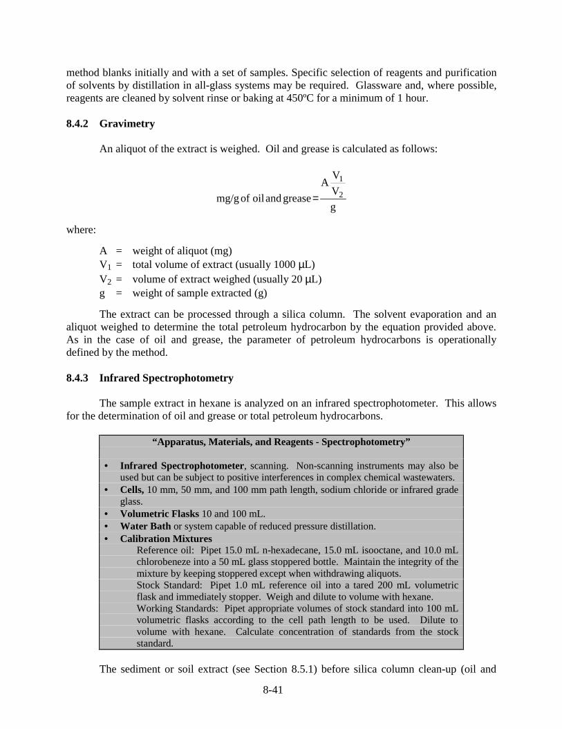
8-41

method blanks initially and with a set of samples. Specific selection of reagents and purificationof solvents by distillation in all-glass systems may be required. Glassware and, where possible,reagents are cleaned by solvent rinse or baking at 450ºC for a minimum of 1 hour.

8.4.2 Gravimetry

An aliquot of the extract is weighed. Oil and grease is calculated as follows:

g

V

VA

greaseandoilofmg/g 2

1

=

where:

A = weight of aliquot (mg)V1 = total volume of extract (usually 1000 µL)V2 = volume of extract weighed (usually 20 µL)g = weight of sample extracted (g)

The extract can be processed through a silica column. The solvent evaporation and analiquot weighed to determine the total petroleum hydrocarbon by the equation provided above.As in the case of oil and grease, the parameter of petroleum hydrocarbons is operationallydefined by the method.

8.4.3 Infrared Spectrophotometry

The sample extract in hexane is analyzed on an infrared spectrophotometer. This allowsfor the determination of oil and grease or total petroleum hydrocarbons.

“Apparatus, Materials, and Reagents - Spectrophotometry”

• Infrared Spectrophotometer, scanning. Non-scanning instruments may also beused but can be subject to positive interferences in complex chemical wastewaters.

• Cells, 10 mm, 50 mm, and 100 mm path length, sodium chloride or infrared gradeglass.

• Volumetric Flasks 10 and 100 mL.• Water Bath or system capable of reduced pressure distillation.• Calibration Mixtures

Reference oil: Pipet 15.0 mL n-hexadecane, 15.0 mL isooctane, and 10.0 mLchlorobeneze into a 50 mL glass stoppered bottle. Maintain the integrity of themixture by keeping stoppered except when withdrawing aliquots.Stock Standard: Pipet 1.0 mL reference oil into a tared 200 mL volumetricflask and immediately stopper. Weigh and dilute to volume with hexane.Working Standards: Pipet appropriate volumes of stock standard into 100 mLvolumetric flasks according to the cell path length to be used. Dilute tovolume with hexane. Calculate concentration of standards from the stockstandard.

The sediment or soil extract (see Section 8.5.1) before silica column clean-up (oil and

8-42

grease) or after silica clean-up (TPH) is diluted to 10 mL or 100 mL.

Select appropriate working standards and cell path length according to the following tableof approximate working ranges:

Path Length Range

10 mm 2-40 mg50 mm 0.4-8 mg

100 mm 0.1-4 mg

Scan standards and samples from 3200 cm-1 to 2700 cm-1 with hexane in the referencebeam and record the results. The absorbances of samples and standards are measured byconstructing a straight baseline over the range of the scan and measuring the absorbance of thepeak maximum at 2930 cm-1 and subtracting the baseline absorbance at that point. For anexample of a typical oil spectrum and baseline construction (see Gruenfeld 1973). Non-scanninginstruments should be operated according to manufacturer’s instructions although calibrationmust be performed using the standards described above. If the absorbance exceeds 0.8 for asample, select a shorter pathlength or dilute as required.

Use a calibration plot of absorbance vs. mg oil prepared from the standards to determinethe mg oil in the sample solution.

Calculation: mg/g total oil and grease = (R x D)/g

where:

R = response factor for oil in solution, determined from calibration plot, in milligramsD = extract dilution factor, if used.g = grams of sediment extracted.

8.4.4 Gas Chromatography

The determination of total petroleum hydrocarbons (TPH) can provide an initialscreening method to determine the extent of petroleum, coal tar, creosote, refined oil, etc.contamination. This method is applicable to sediments, soils, water, wastewater, seawater, andsnow after sample extraction. If there is a specific product spill (e.g., diesel fuel), that productcan be used as a standard, making the method specific for that product. The detection limit forthis method is 200 µg/g or mg/L. When this method is used to analyze samples for which thereis no reference diesel oil, diesel oil identification should be supported by at least one additionalqualitative technique, i.e., gas chromatograph/mass spectrometer (GC/MS). The detection limitof this method is usually dependent upon the presence of other oils in the sample. Excludinginterferences, estimated detection limits of 200 mg/kg of total oil and 100 mg/kg of diesel can beobtained.

Samples are extracted as described in Section 8.5.1 The extract is dried by passagethrough sodium sulfate. A subaliquot of the extract is evaporated to dryness, and the totalamount of oil in the sample is determined gravimetrically. The oil, together with a measured

8-43

volume of internal standard, is redissolved in a known volume of methylene chloride, and analiquot is injected into a gas chromatograph (GC). The components of the oil are separated bythe GC and detected using a flame ionization detector (FID). Identification of diesel oil(qualitative analysis) is performed by comparing the pattern of GC peaks (retention times andintensities) from the sample extract with the pattern of GC peaks from a reference diesel oilsample. Identification of diesel oil is established when the reference diesel and sample patternsagree per the criteria in this method. Quantitative analysis of diesel oil is performed using aninternal standard technique.

There is no standard diesel oil. Oil components, as seen by GC/FID, will differdepending upon the oil source. For rigorous identification and quantification of diesel oil in afluid sample by GC/FID, the chromatographic pattern from the diesel oil should be matched withthe chromatographic pattern from a reference standard of the same diesel oil suspected to be inthe sample.

“Apparatus, Materials, and Reagents - TPH-Gas Chromatography”

• Bottle: Boston round wide-mouth jar with PTFE-lined screw-cap (Sargent WelshS-9184-72CA, or equivalent). New bottles are used as received with no furthercleaning required.

• Glass wool: Pyrex (Corning 3950, or equivalent). Solvent-extracted or baked at450ºC for a minimum of 1 hour.

• Separatory funnel: 60-mL with PTFE stopcock.• Drying column: Pyrex chromatographic column, 400 mm long by 15 to 20 mm

i.d., equipped with coarse-glass frit or glass-wool plug.• Glass filtering funnel: Crucible holder (Corning No. 9480, or equivalent).• Spatulas: Stainless steel or PTFE.• Evaporation flask: 500-mL (Kontes K-570001-0500, or equivalent), attached to

concentrator tube with springs (Kontes K-662750-0012).• Concentrator tube: l0-mL, graduated (Kontes K-570050-1025, or equivalent)

with calibration verified. Ground-glass stopper (size 19/22 joint) is used to preventevaporation of extracts.

• Snyder column: Three-ball macro (Kontes K-503000-0232, or equivalent).• Snyder column: Two-ball micro (Kontes K-469002-02 19, or equivalent).• Boiling chips: Teflon, pre-rinsed with methylene chloride.• Glass or silicon carbide: Approximately 10/40 mesh, extracted with methylene

chloride and baked at 450ºC for a minimum of 1 hour.• PTFE (optional): Extracted with methylene chloride.• Water bath: Heated, with concentric ring cover, capable of temperature control

(±2ºC), installed in a fume hood.• Sample vials: Amber glass, 1- to 5-mL with PTFE-lined screw- or crimp-cap, to fit

GC autosampler.• Analytical balance: Capable of weighing 0.1 mg. Calibration must be verified

with class S weights each day of use.• Top-loading balance: Capable of weighing 10 mg.• Sodium sulfate: Anhydrous, ACS grade, granular.

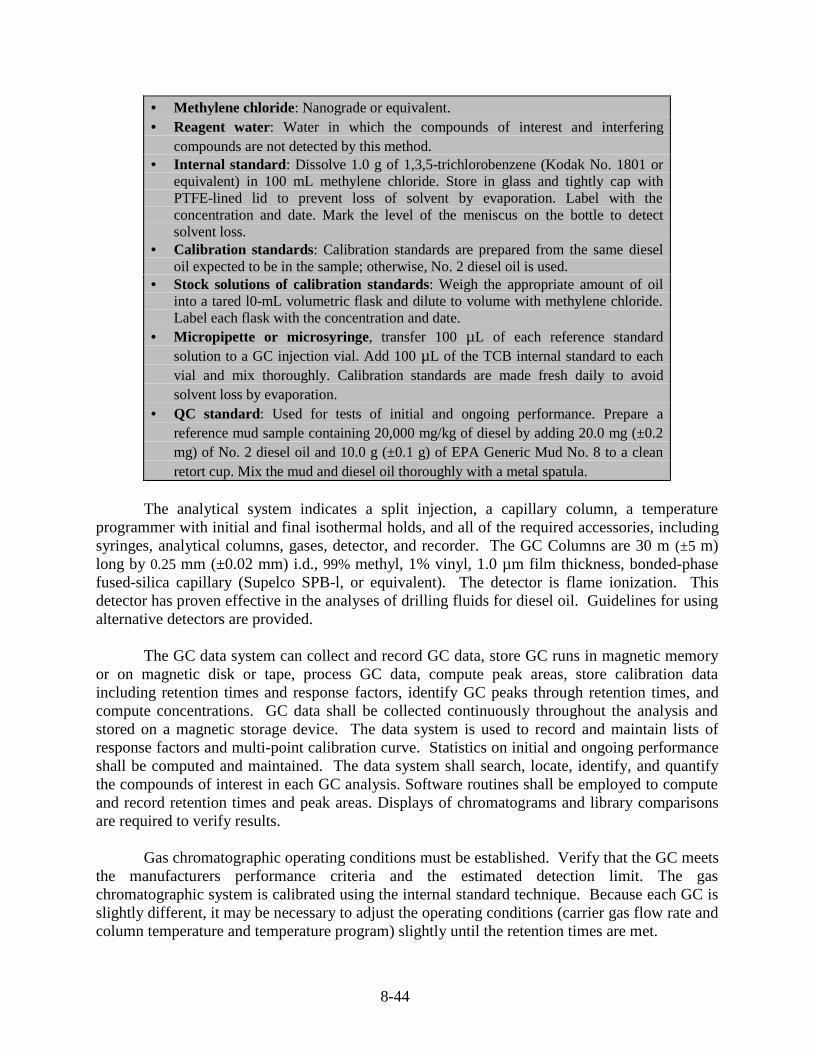
8-44

• Methylene chloride: Nanograde or equivalent.• Reagent water: Water in which the compounds of interest and interfering

compounds are not detected by this method.• Internal standard: Dissolve 1.0 g of 1,3,5-trichlorobenzene (Kodak No. 1801 or

equivalent) in 100 mL methylene chloride. Store in glass and tightly cap withPTFE-lined lid to prevent loss of solvent by evaporation. Label with theconcentration and date. Mark the level of the meniscus on the bottle to detectsolvent loss.

• Calibration standards: Calibration standards are prepared from the same dieseloil expected to be in the sample; otherwise, No. 2 diesel oil is used.

• Stock solutions of calibration standards: Weigh the appropriate amount of oilinto a tared l0-mL volumetric flask and dilute to volume with methylene chloride.Label each flask with the concentration and date.

• Micropipette or microsyringe, transfer 100 µL of each reference standardsolution to a GC injection vial. Add 100 µL of the TCB internal standard to eachvial and mix thoroughly. Calibration standards are made fresh daily to avoidsolvent loss by evaporation.

• QC standard: Used for tests of initial and ongoing performance. Prepare areference mud sample containing 20,000 mg/kg of diesel by adding 20.0 mg (±0.2mg) of No. 2 diesel oil and 10.0 g (±0.1 g) of EPA Generic Mud No. 8 to a cleanretort cup. Mix the mud and diesel oil thoroughly with a metal spatula.

The analytical system indicates a split injection, a capillary column, a temperatureprogrammer with initial and final isothermal holds, and all of the required accessories, includingsyringes, analytical columns, gases, detector, and recorder. The GC Columns are 30 m (±5 m)long by 0.25 mm (±0.02 mm) i.d., 99% methyl, 1% vinyl, 1.0 µm film thickness, bonded-phasefused-silica capillary (Supelco SPB-l, or equivalent). The detector is flame ionization. Thisdetector has proven effective in the analyses of drilling fluids for diesel oil. Guidelines for usingalternative detectors are provided.

The GC data system can collect and record GC data, store GC runs in magnetic memoryor on magnetic disk or tape, process GC data, compute peak areas, store calibration dataincluding retention times and response factors, identify GC peaks through retention times, andcompute concentrations. GC data shall be collected continuously throughout the analysis andstored on a magnetic storage device. The data system is used to record and maintain lists ofresponse factors and multi-point calibration curve. Statistics on initial and ongoing performanceshall be computed and maintained. The data system shall search, locate, identify, and quantifythe compounds of interest in each GC analysis. Software routines shall be employed to computeand record retention times and peak areas. Displays of chromatograms and library comparisonsare required to verify results.

Gas chromatographic operating conditions must be established. Verify that the GC meetsthe manufacturers performance criteria and the estimated detection limit. The gaschromatographic system is calibrated using the internal standard technique. Because each GC isslightly different, it may be necessary to adjust the operating conditions (carrier gas flow rate andcolumn temperature and temperature program) slightly until the retention times are met.

8-45

Tabulate the peak area responses against concentration for each of the ten largest peaks inthe chromatogram (excluding the solvent peak, the internal standard peak, and any peaks thatelute prior to the internal standard peak). Calculate response factors (RF) for each peak using thefollowing equation:

)C)(A(

)C)(A(RF

sis

iss= Equation 1

where:

As = Area of the analyte.Cis = Concentration of the internal standard, in mg/kg.Ais = Area of the internal standard peak.Cs = Concentration of the peak to be measured, in mg/kg.

If the RF is constant (<15% CV) over the calibration range, the RF can be assumed to beinvariant and the average RF can be used for calculations. Alternatively, the results can be usedto plot a calibration curve of response ratios, As/Ais vs. RF.

Calibration verification: For each peak, the average RF or a point on the calibration curveshall be verified on each working day by the measurement of one or more calibration standards.If the RF for any peak varies from the RF obtained in the calibration by more than + 15%, thetest shall be repeated using a fresh calibration standard. Alternatively, a new calibration curveshall he prepared.

Combined response factor: To reduce the error associated with the measurement of asingle peak, a combined response factor is used for computation of the diesel oil concentration.This combined response factor is the sum of the individual response factors as given inEquations 2 or 3:

RF Combined RF(1) + RF(2)... + RF(n) Equation 2

)C)(A(

)C](A...AA[CombinedRF

sis

is)n(s)(s)(s ++= 21

Equation 3

where:

n = Number of individuals peaksAs(l)...A(n) = Areas of the individual peaksCis = Concentration of the internal standard, in mg/kgAis = Area of the internal standard peakCs = Concentration of the peak to be measured, in mg/kg

The analyst shall make an initial demonstration of the ability to generate acceptableaccuracy and precision with this method. This ability is established as described. The analyst ispermitted to modify this method to improve separations or lower the costs of measurements,

8-46

provided all performance requirements are met. Each time a modification is made to the method,the analyst is required to achieve the estimated detection limit. Analyses of spiked samples arerequired to demonstrate method accuracy. Analyses of duplicate samples are required todemonstrate method precision. Analyses of blanks are required to demonstrate freedom fromcontamination. The laboratory shall, on an ongoing basis, demonstrate through calibrationverification and analysis of the QC standard that the analysis system is in control. Thelaboratory shall maintain records to define the quality of data that is generated.

8.5 Polycyclic Aromatic Hydrocarbons

Assessment of the environmental impact of hydrocarbons can require the measurement ofsubstituted and unsubstituted polynuclear aromatic hydrocarbon compounds (PAH) at tracelevels (ng/g or µg/L). These standard operating procedures provide precise and accuratemethods to quantitatively determine petroleum related compounds in snow (water) andsoils/sediments. Acidified water samples are serially extracted with methylene chloride in aseparatory funnel. The extract is dried and concentrated. An optional alumina column cleanupstep is provided for use before the instrumental analysis to remove matrix interferences. Theprotocol is designed for 2-L water samples, but water samples of other sizes may be collectedand extracted by appropriately adjusting the volume of methylene chloride used for theextraction.


The following procedure is a modification of EPA SW846 Method 3540 and Method3611 for Soxhlet extraction of the petroleum hydrocarbon compounds from sediments andextract purification by alumina column chromatography. Ten to thirty grams of chemically driedor oven dried sediment is Soxhlet extracted with methylene chloride and the extract isconcentrated and purified using EPA Method 3611 alumina column purification to removematrix interferences. The alumina purification procedure is usually required prior to analysis.The aliphatic and aromatic fractions are collected in a single fraction. The purified extract isthen submitted for analysis of aliphatic and aromatic hydrocarbons.

Sediment should be collected in precleaned glass jars, or core liners and frozen (-20°C) inthe field. Sediment samples are shipped frozen to the laboratory and stored at -20°C untilanalysis. After subsampling excess sample is archived at -20°C in the dark. Sample extracts arestored in the dark at or below 4°C.

Method interferences may be caused by contaminants in solvents, reagents, glassware,and other sample processing hardware (i.e., freeze dryers) that lead to false positives in GC/FIDor GC/MS detection. All materials used in this method are routinely demonstrated to be freefrom interferences by processing procedural blanks consisting of combusted sand with wateradded through the entire analytical procedure including freeze drying (one blank per 20 samplesor each batch, whichever is more frequent). Field blanks are sometimes also analyzed to see ifcontamination has occurred during sampling. These blanks, when available, will be run withtheir respective sample batches through the entire analytical procedure.

Matrix interferences result from co-extraction of compounds other than the analytes ofinterest. Elemental sulfur and naturally occurring materials can cause interferences in the

8-47

analysis of sediment extracts. Alumina cleanup with activated copper is used to purify thesample prior to analysis.

Glassware is cleaned by detergent (micro cleaning solution) washing with water andrinsing with tap water. The glassware is then combusted in a muffle furnace at 400°C for at least4 hours. Solvent rinses of acetone to dry followed by methylene chloride may be substituted forthe muffle furnace heating when determined to be appropriate by the analyst. After drying andcooling, glassware is sealed and stored in a clean environment to prevent the accumulation ofdust or other contaminants. Stored glassware is maintained capped with combusted aluminumfoil.

“Apparatus, Materials, and Reagents - PAH”

• Glass Jars: 250 mL or 500-mL glass jars, or other suitable containers.• Vials: 1-mL to 7-mL glass vials with Teflon-lined caps.• Glass Funnels• Flat Bottom Flasks: 250 and 500 mL.• Soxhlet Extractor Flasks: 40 mm ID and condensor.• Thimbles: Aluminum, medium or coarse, 44-mL round bottom.• Concentrator Tube: Kuderna-Danish - 25 mL, graduated. Ground glass stoppers

are used to prevent evaporation of extracts.• Snyder Column: Kuderna-Danish - Three ball column.• Micro Reaction Vessels: 2.0 mL or 1.0 mL autosampler vials with crimp cap

septa.• Chromatographic Column: 300-mm x 10-mm inner diameter, with Pyrex glass

wool at bottom and Teflon stopcock.• Analytical Balance: Capable of weighing to 0.0001 mg.• Analytical Balance: Capable of weighing to 0.1 g.• Water Bath: Heated to 60°-70°C.• Teflon Boiling Chips: Solvent extracted.• Syringes: 10 or 25 µL.• Disposable Glass Pasteur Pipettes: 1-mL.• Pyrex Glass Wool: Combusted to 400°C.• Nitrogen Gas Evaporation Unit

Note: Volumetric glassware for sample measurement or introduction of internalstandards must be calibrated.

• Reagent Water: Reagent water contains no analytes above the method detectionlimit.

• Sodium Sulfate: (ACS) Granular, anhydrous (purified by heating at 400ºC for 4 hin a shallow tray or other suitable method).

• Solvents: Hexane, methylene chloride (pesticide quality or equivalent).• Alumina: Neutral 80-325 MCB chromatographic grade or equivalent. Combust

alumina at 400°C for 4 hr and store at 120°C prior to use.• Activated Copper Turnings• Granular Copper• Surrogate Spiking Solutions• Matrix Spike Standard• Internal Standard Solution

8-48

A subsample (~1 g) is weighed, oven-dried and reweighed to obtain percent moisture.The rest of the sample is also oven- or chemically-dried unless a frozen archive sample isneeded. The oven-dried sample is homogenized by mortar and pestle and an aliquot (10 g) isremoved and accurately weighed for analysis. Alternatively, a weighed aliquot (10-30 g) of thesample is chemically-dried by mixing the sample with 30-100 g of sodium sulfate, addingadditional sodium sulfate until the sample is dry, free-flowing and homogeneous. Core samplesor sections are processed by extruding the frozen core after slightly warming the outside liner.Add the sample to an extraction thimble and place the thimble into the Soxhlet holder. A ball ofcopper wire of about 3 centimeters diameter is cleaned in 10% HCl, then water, methanol, andmethylene chloride. One ball is placed in each 250 mL extraction flask. Add 150 mL ofmethylene chloride to the extraction flask containing 1 or 2 boiling chips. Add 50 mL ofmethylene chloride to the sediment in the thimble. Add surrogates to the CH2Cl2 wettedsediment in the thimble. Spike with PAH surrogates. Attach the 250 mL flat bottom flask andextract the sample for 4 to 8 hours. Recycling should occur every 4 minutes. If necessary, filterand dry the extract with glass wool and sodium sulfate. Concentrate the extract by Kuderna-Danish techniques to 4-5 mL. Transfer to a 25 mL concentrator tube. Rinse the flat bottom flaskthree times with 2 mL of methylene chloride and transfer the rinse to the concentrator tube.Concentrate the extract and exchange the solvent to 2.0 mL hexane.

Alumina column clean-up is usually recommended. Place a plug of combusted glasswool in the bottom of the glass chromatographic column. Add 1-1/2 centimeters of combustedquartz sand to cover the glass wool. Fill the reservoir with hexane and add 10.0 g alumina.Gently tap the column to distribute the alumina evenly. Alternatively, a slurry of alumina inhexane may be used to pack the column. Allow the alumina to settle and then add 1.0 g ofanhydrous sodium sulfate on top of the alumina and 10.0 g of activated copper. Drain thehexane and elute the column with 50 mL of hexane. Drain the column until the head of theliquid in the column is just above the sodium sulfate layer. Transfer the sample extract onto thecolumn. Rinse the extract vial with 1 mL methylene chloride and add it to the columnimmediately. To avoid overloading the column, it is suggested that no more than 200 mg ofextract should be placed on the column. Add 100 mL methylene chloride, and elute at a flowrate of 2 mL/min. Collect the effluent in a 250 mL flat bottom flask. The collected fractioncontains aliphatic and aromatic hydrocarbons. Concentrate the extract to 0.5 mL hexane.

Reporting units are ng/g (wet or dry weight). The detection limit for the method is 4,000ng/g for the unresolved complex mixture, 3 ng/g for individual alkanes and isoprenoids, and 1ng/g for individual PAH compounds based on dry sample weight. The performance can beadjusted by decreasing final sample volume, increasing sample amount and/or increasing volumeinjected.

8.5.2 Spectrophotometry

A semi-quantitative estimate of aromatic hydrocarbons can be obtained with theultraviolet/fluorescence procedure but the analyst is reminded of the limitations due to possibleinterference of non-hydrocarbon organic compounds. The procedures described here are fromUnited Nations Environment Program (1992).

8-49

The fluorometer must be capable of synchronous scanning of excitation and emissionwavelengths and be connected to a recorder or data system. The fluorometer is first tested for itssignal to noise ratio and the accuracy of the monochromators by following the instructions in theinstrument manual. This procedure is briefly described below. The hexane used for samplepreparation is then tested for its contribution to blank signals. Aliquots of sample fractions inhexane are then scanned. Emission scans and synchronous excitation/emission scans arerecorded and evaluated for the type of aromatic hydrocarbons in the samples. Standard responsecurves of fluorescence intensity versus concentration are generated for appropriate oil standardsand for the standard aromatic hydrocarbon, chrysene. The sample fractions are diluted to give areading within the linearly calibrated range of the fluorometer. Aliquots of the hexane solutionsof blanks, standards, and samples are pipetted in turn into a quartz fluorometer cell. All blanks,standards, and samples should be run at identical instrument settings and conditions and usingthe same batch of pre-tested hexane.

The signal to noise ratio is tested as follows. Turn on the xenon lamp and allowinstrument to warm up for about 30 minutes. Set controls:

mode: ENERGY (electronic filtering mechanism turned off)response: NORM (2.0 sec)GAIN switch: NORM (750 V)

Carefully fill the 10 mm quartz cell with distilled water ensuring that there are nobubbles, and position the cell in the sample compartment. Set the following conditions:

EMISSION SLIT: 10 nmEXCITATION SLIT: 10 nmSAMPLE SHUTTER: openEMISSION WAVELENGTH: 397 nmEXCITATION WAVELENGTH 350 nmSCAN SPEED: 60 nm/min

By turning the coarse and fine SENSITIVITY knobs, deflect the recorder pen to about80% of full scale at 397 nm (Range typically 3.0 or 1.0).

Set EMISSION WAVELENGTH dial at 300 nm. Record the emission spectrum of thedistilled water from 330 nm to about 500 nm. Turn off the WAVELENGTH DRIVE andmanually scan back to the emission maximum of the Raman band which should be at 397 nm.Record the noise level at this maximum. Measure the signal height of the Raman peak from thefloating baseline to the peak height. Measure the height of the noise. The signal to noise ratioshould be 80/1 or greater (Figure 8.1). Keep a running log of signal to noise ratios and hours ofuse on the xenon lamp. Replace the lamp when its signal to noise ratio is unsatisfactory. Note:Follow all precautions in the instrument manual for handling and aligning new lamps. Usegloves and never touch the lamps with your fingers. Wear protecting cobalt eye glasses ifnecessary to view a lighted UV lamp.

The instrument manual will have more tests for stability and wavelength accuracy.Follow these instructions to become familiar with the operation and performance of thefluorometer.

8-50

Figure 8.1. Rayleigh and Raman scatter plus signal to noise ratio (from UNEP 1992).

8-51

For the fluorescence analysis, samples are dissolved in hexane. The complete proceduralblank value is acceptable for sample correction if its fluorescence reading does not exceed twicethe fluorescence reading of the unconcentrated hexane.

One set of standards should be chrysene in hexane and some intercalibration programshave reported results in terms of chrysene units. Construction of this calibration curve will thusaid in the intercomparison of data sets. However, before the standard chrysene can be used forcalibration, its correct emission spectrum must be verified. This is done by exciting the chrysenesolution at 310 nm and recording its emission spectrum. The correct spectrum will show anemission maximum near 362 nm and 381 nm and a smaller maximum near 408 nm.

A hexane stock solution is prepared by dissolving 1l0 mg chrysene per 100 mL ofhexane. Note that although the chrysene is quite soluble at this concentration, the kinetics ofdissolution are slow. Thus the stock solutions must stand at least 12 hrs before dilution. Fromthe stock solution a range of dilutions is prepared. The required range will depend on thesensitivity of the fluorometer. Under the conditions specified for the analysis, moderninstruments will give a linear response up to a chrysene concentration of approximately 3 µg/mL.20 mL glass scintillation vials with aluminum foil lined lids are useful vessels for the preparationof standard dilutions. The necessary volume of stock solution is pipetted into the preweighedvial which is partially filled with hexane. The volume is then brought up to 20 mL with hexane(1.0 mL of hexane weighs 0.6603 g).

Standard solutions should also be prepared from refined or crude oils. Oil standards areprepared in much the same way as the chrysene standards. The density of the oil in g/mL isdetermined by weighing a measured volume of oil. Then enough oil is transferred to the 100 mLvolumetric stock flask to yield a concentration of approximately 0.5 mg oil per mL of hexane.This stock solution is then used to prepare the standard dilutions in the linear calibration range.This is usually in the 0 to 10 µg/mL range for most oils, but will vary depending on the aromaticcontent of the soil. Some oils, such as Kuwait crude, are difficult to dissolve and will requirethat the primary stock solution is much less concentrated than the average values given here. Theoil standards are run in the fluorometer at the same sensitivity settings as the chrysene standards.

When reporting results in terms of oil units, an intercomparison ratio between thefluorescence intensity of the oil and that of chrysene should be calculated according to theformula:

g/mLin standard chrysene ofion concentrat

g/mLin standard oil ofion concentrat x

standard oil ofintensity cefluorescen

chrysene ofintensity cefluorescen R

µµ=

The choice of oils used for calibration and the wavelengths for the quantitativemeasurement will depend on the types of oil seen in samples from individual monitoringprograms. The analyst should compile a “library” of spectra and response curves generated fromthe particular instrument used.

For qualitative identification of oil type based on the fluorescence of aromatichydrocarbon components, a synchronous excitation/emission scan provides the best resolutionwith elimination of spectral interferences due to Rayleigh and Raman scattering. The excitation

8-52

monochomator is set 23 nm below the emission wavelength and the two monochromators arescanned synchronously (start with excitation at 237 nm and emission at 260 nm). Set theexcitation monochromator slits (or band pass widths) at 10 nm and emission monochromatorslits at 3 to 5 nm depending on instrument sensitivity. Set scan speed at 50 nm/min and recorderspeed at 3 or 6 cm/min. Record synchronous spectra between 260 nm and about 525 nmemission. Examples of synchronous excitation-emission spectra generated from standard oils andextracts from sediment contaminated with oil, using a Perkin Elmer 650 instrument are shown inFigure 8.2. Notations for the emission region of single through five ringed compounds are takenfrom Popi et al. (1975). Inspection of these spectra indicate that diesel oil contains mostlysubstituted naphthalenes and no signal due to the higher ringed aromatics. Crude oils showmaxima in higher wavelength regions. Microbial degradation of the side chains on the aromaticrings will shift emission maxima to shorter wavelengths (as much as 15 nm), whereas solutionprocesses will preferentially remove the more soluble single and double ring components. Thusfor accurate interpretation the analyst must be familiar not only with the characteristic spectragenerated by standard oils, but also with the effects of weathering processes in altering thefluorescence spectra.

When the oil in samples has been matched as closely as possible to the availablestandards, then this standard can be used for constructing the calibration curve. First determinethe optimum wavelengths for the quantitative measurement. This is achieved by fixing theemission wavelength and obtaining an excitation spectrum. The wavelength of optimumexcitation is then chosen and fixed and an emission spectrum obtained. The most sensitivewavelengths would then be those empirically determined from the excitation and emissionspectra. For average crude oils these optima are at 310 nm excitation and 360 nm emission. Fordiesel oil these optima are at 280 nm and 327 nm, respectively (280 nm/327 nm).

Calibration curves are constructed by setting the excitation and emissionmonochromators at 310 nm and 360 nm respectively for chrysene and most crude oils. Thestandard dilutions or stock aliquots are pipetted into the 10 mm cell and the fluorescenceintensity (FI) measured. A plot of FI vs µg/mL should be constructed and the regressionequation calculated over the linear range as per Figure 8.3. Calibrations should be obtained dailyand a running log kept. As aliquots are removed from the stock vials, the vials should bereweighed to ensure no solvent loss, and hence no change in concentration. New dilutionsshould be prepared on a routine basis.

A quick alternative method for constructing calibration curves is prepare the standard oilsolutions to a stock concentration of approximately 0.2 mg/mL for most medium weight crudeoils or 1 mg/mL for less fluorescent oils such as diesel fuel. The calibration curve is thenconstructed by placing 2 mL of hexane into the cuvette and taking the blank reading at theappropriate wavelengths and instrument settings. Sequential 10 µL or 5 µL aliquots of the stockoil solutions are then added to the cuvette, the sample mixed and a reading taken after eachaddition.

The FI of each sample (total extractable lipids or the aromatic fractions of sampleextracts) is determined and the concentration of oil determined from the standard curve.Samples must be diluted to produce readings in the linear region. This is easily done by theprocedure of placing 2 mL hexane in the cell and adding sample extract in µL aliquots. The

8-53

Figure 8.2 Synchronous excitation/emission fluorescence spectra of aromatic hydrocarbonfractions of: (A) source oils and (B) Environmental samples. Scan from 260 to 540emission with excitation set 23 nm lower. Band pass 5 nm. (a) hexane blank, (b)diesel oil, (c) lube oil, (d) Gippsland crude oil, (e) mussels from refinery wharf, (f)clean mussels, (g) mussels from boat wharf, (h) sediments near refinery, and (i)clean sediments (from UNEP 1992).

8-54

Figure 8.3. Calibration graph: degraded VMI crude oil 310/360 nm (from UNEP 1992).

sample dilutions must be recorded (dilution is total µL sample extract divided by the µL used forFI determination. If any correction must be applied for only a portion of the extract brought tothis stage of the analysis, it must also be applied to the dilution). The semi-quantitative estimateof oil content is calculated from the regression line and expressed as µg/mL. Sample content isthen calculated as follows:

weightdrygxdilutionxmLx

mL

g

weightdryg

)chryseneor(oilg 12

µ=µ

The results are reported in µg/g “chrysene or oil equivalents”. If the sample extract hasbeen fractionated into hydrocarbon classes, the intensity of fluorescence of each fraction willdepend on the relative amounts of single through five and heavier ringed aromatics in thefractions. An example of the relative distribution of FI measured at 210 nm/360 nm betweenfractions from the column chromatography separation of a few standards oils are listed below:

(F1) (F2) (F3)

Venez/Mex Ismus Crude Oil 4% 48% 20%Gippsland Crude Oil 5% 53% 42%Marine Diesel Oil 0% 93% 7%Lubricating Oil 16% 44% 40%

8-55

The intensity of the emitted fluorescence is a function of the character of the fluorescentcompounds in a sample, their concentrations, the dimension of the sample in the light path of thephotometer, and also of the intensity of the excitation source.

There is a linear relationship between the sample concentration of fluorescing compoundsand the intensity of the emitted light only within certain limits when the total absorbance of thesample is low. If the absorbance exceeds 0.05 absorbance units (less than 95% transmittance), FIwill be reduced by the presence of any compound in the sample that can absorb either theexcitation light or the emitted light. As this effect takes place in the sample cell, the disturbanceis called an “inner filter effect”. At high concentration this can be caused by the fluorescingcompound itself. This is common in highly polluted sample extracts. Other compounds co-extracted with the oil may also cause a reduction in emitted light by “quenching”. In thisinstance the energy is transferred to the co-extracted substances or “quenchers,” rather than beingemitted as a fluorescence emission.

The following tests can be used to test for inner filter effects. None of these experimentsare fully conclusive and a good knowledge of fluorometry is necessary for their application andeffective evaluation.

This test can help to reveal inner filter effects but not quenching. The test will work onlyif the Raman scattering peak is separated from the emission band of the petroleum hydrocarbons.If the Raman peak is superimposed on the slope of any other emission peak, the test is notconclusive.

Use 270 nm as the excitation wavelength. Fill the cell with pure hexane. Scan,mechanically or manually, the emission spectrum to find the maximum of the Raman scatteringwhich should occur at 297 nm (to resolve the Rayleigh from the Raman scatter, narrow slits andhigh sensitivity settings must be used). Record the spectrum. Replace the hexane with thesample and scan in the same way to record the Raman scatter. It should be of the same intensityas that from the pure hexane. If it is significantly lower, an inner filter effect is present and thesample must be diluted and/or subject to an adsorption chromatography clean-up procedure.

Make a series of measurements of FI (310 nm/360 nm) of the sample at differentdilutions. Plot FI vs the diluted concentrations. If a straight line is obtained there is no innereffect and any of the measurements can be used for quantification. If the relationship is notlinear, dilute the sample until a linear relationship is obtained and use the FI at these dilutions forthe quantification. For routine purposes, a single dilution can be used provided the results agreewithin 20%.

Measure the FI of the sample, then dilute it with an equal volume of a standard ofchrysene or oil solution that has the same FI as the sample. Then measure the FI of the sampleplus standard mixture. The FI of the mixture should be equal to:

FI of mixture = (FI of standard)/2 + (FI of sample)/2

If the FI of the mixture is less than that predicted by more than 20%, then significantinner filter effects exist and the FI of the sample must be multiplied by this correction factor forthe quantification.

8-56

Note: The synchronous excitation/emission scan is much more selective to aromatichydrocarbons by showing less interference from biogenic pigments. It is feasible to quantify byconstructing calibration curves based on synchronous scans. At the time of revision of thismanual, the U.S. Coast Guard Oil Spills Laboratory is experimenting to determine optimumwavelength differences.

8.5.3 High Performance Liquid Chromatography (HPLC)

This method is used to determine the concentration of certain polynuclear aromatichydrocarbons (PAH) in ground water and wastes. Specifically this method is used to detect thefollowing substances:

Analyte CAS#

Acenaphthene 83-32-9Acenaphthylene

Anthracene 120-12-7Benzo(a)anthracene 56-55-3

Benzo(a)pyrene 50-32-8Benzo(b)fluoranthene 205-99-2Benzo(ghi)perylene 191-24-2

Benzo(k)fluoranthene 207-08-9Chrysene 218-01-9

Dibenzo(a,h)anthracene 53-70-3Fluoranthene 206-44-0

Fluorene 86-73-7Indeno(1,2,3-cd)pyrene 193-39-5

Naphthalene 91-20-3Phenanthrene 85-01-8

Pyrene 129-00-0

Use of this method presupposes a high expectation of finding the specific compounds ofinterest. If the user is attempting to screen samples for any or all of the compounds listed above,the analyst must develop independent protocols for the verification of identity. The methoddetection limits for each compound in reagent water are listed in Table 8.9. Table 8.10 lists thepractical quantitation limit for other matrices. The sensitivity of this method usually depends onthe level of interferences rather than instrumental limitations. The limits of detection listed inTable 8.9 for the liquid chromatographic approach represent sensitivities that can be achieved inthe absence of interferences. When interferences are present, sensitivity is decreased.

Prior to the use of this method, appropriate sample extraction techniques must be used(see Section 8.6.1). A 5- to 25-µL aliquot of the extract is injected into an HPLC, andcompounds in the effluent are detected by ultraviolet (UV) and fluorescence detectors. Ifinterferences prevent proper detection of the analytes of interest, the method may also beperformed on extracts that have undergone cleanup using alumina column cleanup (see Section8.5.1).

The chromatographic conditions described allow for a unique resolution of the specificPAH compounds covered by this method. Other PAH compounds in addition to matrix artifacts,may interfere.

8-57

“Apparatus, Materials, and Reagents - HPLC”

• Kuderna-Danish (K-D) apparatusConcentrator tube: 10-mL, graduated (Kontes K-570050-1025 or equivalent). Ground-glass stopper is used to prevent evaporation of extracts.Evaporation flask: 500-mL (Kontes K-570001-500 or equivalent). Attach toconcentrator tube with springs.Snyder column: Three-ball macro (Kontes K-503000-0121 or equivalent).Snyder column: Two-ball micro (Kontes K-569001-0219 or equivalent)Boiling chips: Solvent extracted, approximately 10/40 mesh (silicon carbide orequivalent).Water bath: Heated, with concentric ring cover, capable of temperature control(±5ºC). The bath should be used in a hood.Syringe: 5-mL.High pressure syringes.

• HPLC apparatus:Gradient pumping system: Constant flow.Reverse phase column: HC-ODS Sil-X, 5-micron particle size diameter, in a250-mm x 2.6-mm I.D. stainless steel column (Perkin Elmer No. 089-0716 orequivalent).Detectors: Fluorescence and/or UV detectors may be used.Fluorescence detector: For excitation at 280-nm and emission greater than389-nm cutoff (Corning 3-75 or equivalent). Fluorometers should havedispersive optics for excitation and can utilize either filter or dispersive opticsat the emission detector.UV detector: 254-nm, coupled to the fluorescence detector.Strip-chart recorder: compatible with detectors. A data system for measuringpeak areas and retention times is recommended.Volumetric flasks: 10-, 50-, and 100-mL.Reagent water: Reagent water is defined as water in which an interferent is notobserved at the method detection limit of the compounds of interest.Acetonitrile: HPLC quality, distilled in glass.Stock standard solutions: Prepare stock standard solutions at a concentrationof 1.00 µg/µL by dissolving 0.0100 g of assayed reference material inacetonitrile and diluting to volume in a 10-mL volumetric flask. Largervolumes can be used at the convenience of the analyst. When compound purityis assayed to be 96% or greater, the weight can be used without correction tocalculate the concentration of the stock standard. Commercially prepared stockstandards can be used at any concentration if they are certified by themanufacturer or by an independent source. Transfer the stock standardsolutions into Teflon-sealed screw-cap bottles. Store at 4ºC and protect fromlight. Stock standards should be checked frequently for signs of degradation orevaporation, especially just prior to preparing calibration standards from them.Stock standard solutions must be replaced after one year, or sooner ifcomparison with check standards indicates a problem.Calibration standards: Calibration standards at a minimum of fiveconcentration levels should be prepared through dilution of the stock standardswith acetonitrile. One of the concentration levels should be at a concentrationnear, but above, the method detection limit. The remaining concentration levelsshould correspond to the expected range of concentrations found in realsamples or should define the working range of the HPLC. Calibration

8-58

standards must be replaced after six months, or sooner if comparison withcheck standards indicates a problem.Internal standards (if internal standard calibration is used): To use thisapproach, the analyst must select one or more internal standards that aresimilar in analytical behavior to the compounds of interest. The analyst mustfurther demonstrate that the measurement of the internal standard is notaffected by method or matrix interferences. Because of these limitations, nointernal standard can be suggested that is applicable to all samples. Preparecalibration standards at a minimum of five concentration levels for eachanalyte as described in above. To each calibration standard, add a knownconstant amount of one or more internal standards, and dilute to volume withacetonitrile.Surrogate standards: The analyst should monitor the performance of theextraction, cleanup (if necessary), and analytical system and the effectivenessof the method in dealing with each sample matrix by spiking each sample,standard, and reagent water blank with one or two surrogates (e.g.,decafluorobiphenyl or other PAHs not expected to be present in the sample)recommended to encompass the range of the temperature program used in thismethod. Deuterated analogs of analytes should not be used as surrogates forHPLC analysis due to coelution problems.

Extracts must be stored under refrigeration and must be analyzed within 40 days ofextraction.

Prior to HPLC analysis, the extraction solvent must be exchanged to acetonitrile. Theexchange is performed during the K-D procedures listed in all of the extraction methods. Theexchange is performed as follows.

Following K-D of the methylene chloride extract to 1 mL using the macro-Snydercolumn, allow the apparatus to cool and drain for at least 10 min. Increase the temperature of thehot water bath to 95-100ºC. Momentarily remove the Snyder column, add 4 mL of acetonitrile, anew boiling chip, and attach a two-ball micro-Snyder column. Concentrate the extract using 1mL of acetonitrile to prewet the Snyder column. Place the K-D apparatus on the water bath sothat the concentrator tube is partially immersed in the hot water. Adjust the vertical position ofthe apparatus and the water temperature, as required, to complete concentration in 15-20 min. Atthe proper rate of distillation the balls of the column will actively chatter, but the chambers willnot flood. When the apparent volume of liquid reaches 0.5 mL, remove the K-D apparatus andallow it to drain and cool for at least 10 min. When the apparatus is cool, remove the micro-Snyder column and rinse its lower joint into the concentrator tube with about 0.2 mL ofacetonitrile. A 5-mL syringe is recommended for this operation. Adjust the extract volume to 1.0mL. Stopper the concentrator tube and store refrigerated at 4ºC, if further processing will not beperformed immediately. If the extract will be stored longer than two days, it should betransferred to a Teflon-sealed screw-cap vial. Proceed with HPLC analysis if further cleanup isnot required.

Using the column described, isocratically elute for 5 min using acetonitrile/water(4:6)(v/v), then linear gradient elution to 100% acetonitrile over 25 min at 0.5 mL/min flow rate.If columns having other internal diameters are used, the flow rate should be adjusted to maintaina linear velocity of 2 mm/sec.

8-59

Use Table 8.9 and especially Table 8.10 for guidance on selecting the lowest point on thecalibration curve. Assemble the necessary HPLC apparatus and establish operating parametersequivalent to those indicated in above. By injecting calibration standards, establish thesensitivity limit of the detectors and the linear range of the analytical systems for eachcompound. Before using any cleanup procedure, the analyst should process a series ofcalibration standards through the procedure to confirm elution patterns and the absence ofinterferences from the reagents.

The estimated retention times of PAHs determinable by this method are summarized inTable 8.9. An example chromatogram is shown in Figure 8.1. If internal standard calibration isto be performed, add 10 µL of internal standard to the sample prior to injection. Inject 2-5 µL ofthe sample extract with a high-pressure syringe or sample injection loop. Record the volumeinjected to the nearest 0.1 µL, and the resulting peak size, in area units or peak heights. Re-equilibrate the HPLC column at the initial gradient conditions for at least 10 min betweeninjections. Using either the internal or external calibration procedure, determine the identity andquantity of each component peak in the sample chromatogram which corresponds to thecompounds used for calibration purposes. If the peak area exceeds the linear range of the system,dilute the extract and analyze. If the peak area measurement is prevented by the presence ofinterferences, further cleanup is required.

The quality control check sample concentrate should contain each analyte at thefollowing concentrations in acetonitrile: naphthalene, 100 µg/mL; acenaphthylene, 100 µg/mL;acenaphthene, 100 µg/mL; fluorene, 100 µg/mL; phenanthrene, 100 µg/mL; anthracene, 100µg/mL; benzo(k)fluoranthene, 5 µg/mL; and any other PA at 10 µg/mL.

The calibration and QC acceptance criteria for this method are summarized in Table 8.11.Method accuracy and precision as functions of concentration for the analytes of interest issummarized in Table 8.12. The contents of both Tables should be used to evaluate a laboratory'sability to perform and generate acceptable data by this method.

Calculate surrogate standard recovery on all samples, blanks, and spikes. Determine if therecovery is within limits.

If recovery is not within limits, the following procedures are required.

• Check to be sure there are no errors in calculations, surrogate solutions and internalstandards. Also, check instrument performance.

• Recalculate the data and/or reanalyze the extract if any of the above checks reveal aproblem.

• Reextract and reanalyze the sample if none of the above are a problem or flagthe data as “estimated concentration.”

PERFORMANCE

The method was tested by 16 laboratories using reagent water, drinkingwater, surface water, and three industrial wastewaters spiked at sixconcentrations over the range 0.1 to 425 µg/L. Single operator precision,overall precision, and method accuracy were found to be directly relatedto the concentration of the analyte and essentially independent of thesample matrix. Linear equations to describe these relationships arepresented in Tables 7-12.

8-60

Table 8.9. High Performance Liquid Chromatography of PAH(s)a.

CompoundRetention Time (min) Column Capacity

Factor (K’)Method Detection Limit(mq/L) UV Fluorescence

Naphthalene 16.6 12.2 1.8Acenaphthylene 18.5 13.7 2.3Acenaphthene 20.5 15.2 1.8Fluorene 21.2 15.8 0.21Phenanthrene 22.1 16.6 0.65Anthracene 23.4 17.6 0.64Fluoranthrene 24.5 18.5 0.21Pyrene 25.4 19.1 0.27Benzo(a)anthracene 28.5 21.6 0.013Chrysene 29.3 22.2 0.15Benzo(b)fluoranthene 31.6 24.0 0.018Benzo(k)fluoranthene 32.9 25.1 0.017Benzo(a)pyrene 33.9 25.9 0.023Dibenzo(a,h)anthracene 35.7 27.4 0.030Benzo(ghi)perylene 36.3 27.8 0.076Indeno(1,2,3-cd)pyrene 37.4 28.7 0.043

aHPLC conditions: Reverse phase HC-ODS Sil-X, 5 micron particle size, in a 250-mm x 2.6-mm I.D. stainlesssteel column. Isocratic elution for 5 min using acetonitrile/water (4:6)(v/v), then linear gradient elution to 100%acetonitrile over 25 min at 0.5 mL/min flow rate. If columns having other internal diameters are used, the flowrate should be adjusted to maintain a linear velocity of 2 mm/sec.

Table 8.10. Determination of Practical Quantitation Limits (PQL) for Various Matricesa.

Matrix Factorb

Ground water 10Low-level soil by sonication with GPC cleanup 670High-level soil and sludges by sonication 10,000Non-water miscible waste 100,000

a Sample PQLs are highly matrix-dependent. The PQLs listed hereinare provided for guidance and may not always be achievable.

b PQL = Method Detection Limit X [Factor]. For nonaqueous samples,the factor is on a wet-weight basis.

8-61

Table 8.11. QC Acceptance Criteria.

Parameter Test Conc.(µg/L)

Limit for s(µg/L)

Range for x(µg/L)

Range P,P(s)(µg/L) (%)

Acenaphthene 100 40.3 D-105.7 D-124Acenaphthylene 100 45.1 22.1-112.1 D-139Anthracene 100 28.7 11.2-112.3 D-126Benzo(a)anthracene 10 4.0 3.1-11.6 12-135Benzo(a)pyrene 10 4.0 0.2-11.0 D-128Benzo(b)fluoranthene 10 3.1 1.8-13.8 6-150Benzo(ghf)perylene 10 2.3 D-10.7 D-116Benzo(k)fluoranthene 5 2.5 D-7.0 D-159Chrysene 10 4.2 D-17.5 D-199Dibenzo(a,h)anthracene 10 2.0 0.3-10.0 D-110Fluoranthene 10 3.0 2.7-11.1 14-128Fluorene 100 43.0 D-119 D-142Indeno(1,2,3-cd)pyrene 10 3.0 1.2-10.0 D-116Naphthalene 100 40.7 21.5-100.0 D-122Phenanthrene 100 37.7 8.4-133.7 D-155Pyrene 10 3.4 1.4-12.1 D-140

s = Standard deviation of four recovery measurements, in µg/L.x = Average recovery for four recovery measurements, in µg/L.P, P(s) = Percent recovery measured.D = Detected; result must be greater than zero.

Table 8.12. Method accuracy and Precision as Functions of Concentrationa.

Parameter Accuracy, asrecovery, x’

(µg/L)

Single analystprecision s(r)’

(µg/L)

Overallprecision S’

(µg/L)

Acenaphthene 0.52C+-0.54 0.39x+0.76 0.53x+1.32Acenaphthylene 0.69C-1.89 0.36x+0.29 0.42x+0.52Anthracene 0.63C-1.26 0.23x+1.16 0.41x+0.45Benzo(a)anthracene 0.73+0.05 0.28x+0.04 0.34x+0.02Benzo(a)pyrene 0.56C+0.01 0.38x-0.01 053x-0.01Benzo(b)fluoranthene 0.78C_0.01 0.21x+0.01 0.38x-0.00Benzo(ghf)perylene 0.44C+0.30 0.25x+0.04 0.58x+0.10Benzo(k)fluoranthene 0.59C+0.00 0.44x-0.00 0.69x+0.10Chrysene 0.77C-0.18 0.32x-0.18 0.66x-0.22Dibenzo(a,h)anthracene 0.41C-0.11 0.24x+0.02 0.452+0.03Fluoranthene 0.68C+0.07 0.22x+0.06 0.32x+0.03Fluorene 0.56C-0.52 0.44x-1.12 0.63x-0.65Indeno(1,2,3-cd)pyrene 0.54C+0.06 0.29x+0.02 0.42x+0.01Naphthalene 0.57C-0.70 0.39x-0.18 0.41x+0.74Phenanthrene 0.72C-0.95 0.29x+0.05 0.47xl-0.25Pyrene 0.69C-0.12 0.25x+0.14 0.42x-0.00

x' = Expected recovery for one or more measurements of a sample containing a concentration of C, in µg/L.s(r)' = Expected single analyst standard deviation of measurements at an average concentration of x, in µg/L.S' = Expected interlaboratory standard deviation of measurements at an average concentration found of x, in µg/L.C = True value for the concentration, in µg/L.x = Average recovery found for measurements of samples containing a concentration of C, in µg/L.aCriteria from 40 CFR Part 136 for Method 610. These criteria are based directly upon the method’s performance.Where necessary, the limits for recovery have been broadened to assure applicability of the limits.

8-62

This method has been tested for linearity of spike recovery from reagentwater and has been demonstrated to be applicable over the concentrationrange from 8 x MDL to 800 x MDL with the following exception:benzo(ghi)perylene recovery at 80 x and 800 x MDL were low (35% and45%, respectively). The accuracy and precision obtained will bedetermined by the sample matrix, sample-preparation technique, andcalibration procedures used.

8.5.4 Gas Chromatography/Mass Spectrometry (GC/MS)

This method outlines the procedures used for the quantitative determination ofpolynuclear aromatic hydrocarbons (PAH) in sample extracts using gas chromatography/massspectrometry (GC-MS). The instrumental procedures described in this document are applicableto the quantitative analysis of extracts obtained from water, sediment, soil, tissue, and othersample matrices after appropriate extraction and purification (Section 8.5.1). The PAHs targetcompounds determined by this method and the surrogate used for quantitation (referencesurrogate) are listed in Table 8.13. The analytical method detection limit (MDL) is determinedon an annual basis. MDLs for the multi-analyte groups are estimated as twice the MDL of theparent compound.

The quality control requirements for quantitative analysis are summarized in Table 8.14with details provided in the following sections.

The mass spectrometer performance is checked daily using PFTBA according tomanufacturer’s tuning procedures. These procedures include the checking of peak widths, massaxis calibration, and relative abundances of masses 69, 219, and 502 against manufacturer’srecommended criteria. Isotope abundances are also checked according to the manufacturer’scriteria. Total cycle time (dwell times plus switching times) for all ions within a singledescriptor must be one second or less.

Qualitative identification of target compounds is based on a comparison of the retentiontimes of the target compounds in the calibration curve with the retention time of the targetcompounds found in the sample extract. The retention time of the compound in the extractshould be within ±4 seconds of the average retention time of the authentic compounds in thecalibration standard. The ion current responses for ions used for quantitation and confirmationpurposes must simultaneously reach their maxima (±2 seconds). The ion current responses forthe quantitation and confirmation ions used for the labeled standards must reach maximumsimultaneously (±2 seconds).

The extracted ion current profiles of the quantitation ion (primary m/z) and theconfirmation ion (secondary ion) for each target compound must meet the following QCacceptance criteria. The characteristic masses of each target compound must maximize in thesame scan or within one scan of each other. The retention time of target compounds in thesample must fall within ±4 seconds of the retention time for the authentic compound in thecalibration standards. The relative peak heights of the primary ion compared to the confirmation(or secondary) ion mass for a target compound should fall within ±30 percent of the relativeintensities of these masses in a mass spectrum (Table 8.15) obtained from a reference standard of

8-63

Table 8.13. Polynuclear Aromatic Hydrocarbons of Interest.

Compounds I.S.Reference

SurrogateReference

Compounds I.S.Reference

ReferenceSurrogate

Naphthalene A 1 Fluoranthene B 3C1-Naphthalenes A 1 C1-Fluoranthenesa B 3

C2-Naphthalenes A 2C3-Naphthalenes A 2 Pyrene B 3

C4-Naphthalenesa A 2 C1-Pyrene B 3

Biphenyl A 2 Benzo[a]anthracene B 4Acenaphthylene A 2

Chrysene B 4Acenaphthene A 2 C1-Chrysenea B 4

C2-Chrysenea B 4

Fluorene A 2 C3-Chrysenea B 4

C1-Fluorenesa A 2 C4-Chrysenea B 4

C2-Fluorenesa A 2

C3-Fluorenesa A 2 Benzo[b]fluorantheneBenzo[k]fluoranthene ]-sum

B 4

Dibenzothiophene A 3 Benzo[e]pyrene B 4

C1-Dibenzothiophenesa A 3 Benzo[a]pyrene B 4

C2-Dibenzothiophenesa A 3 Perylene B 5

C3-Dibenzothiophenesa A 3 Indeno[1,2,3-c,d]pyrene B 4

Dibenzo[a,h]anthracene B 4Phenanthrene A 3 Benzo[g,h,i]perylene B 4C1-Phenanthrenes A 3

C2-Phenanthrenesa A 3 Specific Isomers

C3-Phenanthrenesa A 3

C4-Phenanthrenesa A 3 1-methylnaphthalene B 1

2-methylnaphthalene B 1Anthracene A 3 2,6-dimethylnaphthalene B 2

C1-Anthracenesa A 3 2,3,5-trimethylnapthalene B 2

C2-Anthracenesa A 3 1-methylphenanthrene B 3

C3-Anthracenesa A 3

C4-Anthracenesa A 3 Surrogates

Internal Standards Naphthalene-d8 (1)Acenaphthene-d10 (2)

Fluorene-d10 (A) Phenanthrene-d10 (3)Benzo (a) pyrene-d12 (B) Chrysene-d12 (4)

Perylene-d12 (5)

aAlkylated homologues not included in the calibration solution.NOTE: Alkylated phenanthrenes and anthracenes, and alkylated fluoranthenes and pyrenes are quantified together as total alkylated (Cx)

phenanthrene/anthracenes and total alkylated (Cx) fluoranthenes/pyrenes. Only the parent compounds and specific isomers arereported as individual compounds.

8-64

Table 8.14. Summary of QC Requirements for Quantitative Analysis.


- Instrument Calibration Minimum of 5 standards; correlationcoefficient of > 0.99 or % RSDwithin ± 15% for all targetcompounds.

Initial and after any failures ofcontinuing calibrations.

- Instrument Blank Instrument free of interferingcontamination or perform necessarymaintenance.

Prior to analysis of all analyticalbatches.

- Reference Oil Solution Analytes within ± 25% or average oflab certified concentration with noanalytes > 35% or recalibrate.

Prior to analysis of all analyticalbatches.

- Continuing CalibrationVerification (CCV)

Percent difference for all responsefactors within ± 15% or average ofinitial calibration; no single analytegreater than 25% or recalibrate andreanalyze back to last passing CCV.

After daily MS tune; once every 12hours during the analytical sequenceand at end of analytical sequence.

- Surrogate Recovery Recovery of 40 to 120% for allsurrogates. See Section 3.5.6 forcorrective actions.

All samples.

- Method Blank No analytes > 3x MDL. See Section3.5.1 for exceptions to need for re-extraction.

One per QC batch.

- Duplicates (if applicable) RPD < 25% for all analytes > 10xMDL. See Section 3.5.4 forcorrective action.

One per QC batch.

- Matrix Spike, Matrix SpikeDuplicate (if applicable)

% recovery within 40 to 120%.RPD for the spike recoveries shouldbe < 25% for all analytes. SeeSections 3.5.3 for corrective actions.

One per QC batch.

- Standard ReferenceMaterial (if applicable)

Recovery of 80% of certified or non-certified compounds within 30% ofcertified range for those analytes >10x MDL. See Section 3.5.5 forcorrective action.

One per QC batch.

8-65

Table 8.15. Parameters for Target Analytes.

Quantitation Confirmation % Relative Abudnance ofCompound Ion Ions Confirmation Ions

d8-Naphthalene 136 134 15Naphthalene 128 127 15C1-Naphthalenes (including isomers) 142 141 80C2-Naphthalenes 156 141 NAC3-Naphthalenes 170 155 NAC4-Naphthalenes 184 169,141 NAd10-Acenaphthene 164 162 95Acenaphthylene 152 153 15Biphenyl 154 152 30Acenaphthene 154 153 98d10-Fluorene 176 174 85Fluorene 166 165 95C1Fluorenes 180 165 NAC2-Fluorenes 194 179 NAC3-Fluorenes 208 193 NAd10-Phenanthrene 188 184 15

Phenanthrene 178 176 20Anthracene 178 176 20C1-Phenanthrenes/anthracenes 192 191 NAC2-Phenanthrenes/anthracenes 206 191 NAC3-Phenanthrenes/anthracenes 220 205 NAC4-Phenanthrenes/anthracenes 234 219,191 NADibenzothiophene 184 152,139 15C1-Dibenzothiophenes 198 184,197 NAC2-Dibenzothiophenes 212 197 NAC3-Dibenzothiophenes 226 211 NAFluoranthene 202 101 15d12-Chrysene 240 236 30Pyrene 202 101 15C1-Fluoranthenes/pyrenes 216 215 NABenzo [a] anthracene 228 226 20Chrysene 228 226 30C1-Chrysenes 242 241 NAC2-Chrysenes 256 241 NAC3-Chrysenes 270 255 NAC4-Chrysenes 284 269,241 NAd12-Benz (a)pyrene 264 260 20Benzo [b] fluoranthene 252 253,125 30, 10Benzo [k] fluoranthene 252 253, 125 30, 10Benzo (e) pyrene 252 253 30Perylene 252 253 20d12-Perylene 264 260 22Benzo [a] pyrene 252 253, 125 30, 10Indeno[1,2,3-c,d]pyrene 276 277, 138 25,30Dibenzo [a,h] anthracene 278 279, 139 25,20Benzo [g,h,i]pery1ene 276 277, 138 25,20

NA = Not Applicable

8-66

that target compound. A compound that does not meet secondary ion confirmation criteria maystill be determined to be present in a sample after close inspection of the data by the massspectroscopist. Supportive data includes the presence of the secondary ion having a ratio greaterthan ±30 percent of the primary ion which may be caused by an interference with the secondaryion. The data not meeting these criteria are reported but appropriately qualified.

Prior to all analytical sequences, a reference oil solution (~800 ng/L) is analyzed. Thisanalysis is used to define the retention time windows for the multiple analyte groups. Thepatterns within the retention time window for the sample extract are compared to the patternwithin the same window of the reference oil solution. The magnitude of the individual peaksmay not be consistent but the location of the peaks within the window should be similar betweenthe two analyses.

A five-point calibration curve based on response factors is established to demonstrate thelinearity of the detector. The recommended standard concentrations are approximately 20, 100,250, 500, and 1000 ng/mL. The QC acceptance criteria for linearity of the initial calibrationcurve requires that the percent relative standard deviation (RSD) of the response factors for eachcompound in the five calibration standards must be less than or equal to fifteen percent (<15%).If these RSD criteria are exceeded, the linearity of the initial calibration curve can be determinedto be acceptable if the correlation coefficient (r) determined using linear least squares regressionanalyses is greater than or equal to 0.99. The instrument software generates and prints out bothtypes of calibration data for all initial calibration determinations, which are maintained incalibration files with the raw data for that laboratory area. Calibration verification must beperformed at the beginning of each analytical sequence. A calibration verification is alsorequired at the end of a 12 hour shift or at the end of the analytical sequence, whichever is morefrequent. QC acceptance criteria are based upon daily response factors for each compoundwhich are compared to the mean response factors for the initial calibration curve. If the averagedaily response factors for all analytes is within ±15% of the calibration value, analyses mayproceed. If, for any single analyte, the daily response factor exceeds ±25 percent of calibrationvalue, the five-point calibration is repeated before analysis continues and all samples are re-analyzed back to last passing CCV.

The acceptance criteria for QC samples are evaluated within an analytical group.Therefore, failure of one QC sample type does not necessarily cause the entire analytical batch tofail. A method blank is used to demonstrate freedom from contamination in the analyticalprocedure, and is required for each set of 20 or fewer samples. If any of the target compoundsare found in the blank at greater than 3x the MDL, re-extraction of the entire set may be requiredas specified in the following subsections. If any of the target compounds are found in the blankat greater than 3x the MDL, but are not detected in the analytical samples above the MDL, theanalytical data can be reported and must be flagged, but no further action is required. Whentarget compounds are present in the method blank and in the analytical samples at concentrationsabove 3x the MDL and the concentration in a sample is 10x that found in the blank, the blankmust be flagged but sample data are reportable and are not flagged. When target compounds arepresent in the method blank and in the analytical samples at concentrations above 3x the MDLand the concentration in the sample is less than 10x that found in the blank, the sample should bere-extracted and re-analyzed. If no sample remains for re-extraction, the analytical data for thoseanalytes in the blank and samples can be reported but must be flagged.

8-67

A laboratory blank spike (LBS) may be used to estimate analytical accuracy of themethod if inadequate sample is available or if a complex matrix is present. It may be requiredwith each set of 20 or fewer samples (Table 8.16). A laboratory blank spike duplicate (LBSD) isused to estimate both analytical accuracy and precision and may be required for each set of 20 orfewer samples. QC acceptance criteria for the target compound recoveries are that the recoveryfor each target compound falls between 40 and 120%. If the LBSD has been included, therecoveries determined from the LBS and LBSD should agree within an average RPD of <25%.If two or more of the target compounds are outside the QC acceptance criterion, corrective actionmay be indicated. Corrective action may include recalculation and/or reanalysis of the LBS andLBSD, re-extraction of the sample group, or instrument maintenance and/or recalibration. Alaboratory blank spike may be used to demonstrate that the analytical system is in control whenworking with a difficult matrix or sample set.

A matrix spike (MS) sample is used to estimate analytical accuracy in the presence of arepresentative matrix and is normally required for each set of 20 or fewer samples A matrixspike duplicate (MSD) is used to estimate analytical accuracy and precision in the presence of arepresentative matrix and may be required for each set of 20 or fewer samples. QC acceptancecriteria for target compound recoveries in the MS and the MSD is 40 to 120% of the spikedamount. In computing the QC acceptance criterion, only valid spikes will be used. In a validspike, the amount of analyte added is at least as much as was originally present in the sample. Ifa MSD has been included with the analytical batch, the recoveries determined from the MS andMSD samples should agree within a RPD of <25%. The MS and MSD acceptance criterion areadvisory. However, if two or more of the target compounds are outside the QC acceptancecriterion, corrective action may be indicated. Corrective action may include recalculation and/orreanalysis of the MS and MSD, re-extraction of the sample/MS/MSD group, or instrumentmaintenance and/or recalibration.

A sample duplicate (DUP) is used to demonstrate sample homogeneity and analyticalprecision in the presence of a representative matrix and may be required with each set of 20 orfewer samples. QC acceptance criterion for analyte concentrations greater than ten times theMDL is a RPD of <25%. If the RPD is outside the QC acceptance criterion, corrective actionmay be indicated. Corrective action may include recalculation or reanalysis of the DUP and theoriginal sample, instrument maintenance, recalibration, or re-extraction of the analytical batch.

A standard reference material (SRM) is used to demonstrate analytical accuracy and maybe required with each set of 20 or fewer samples. When requested, a standard reference materialis extracted and analyzed with each batch of samples. Acceptable concentrations are defined asthe range of the documented (certified or reference) concentration plus or minus the 95%confidence limits in the certification. The QC acceptance criterion are that 80% of the data formeasured concentrations should be within ±30% of the range of the acceptable concentration foreach target compound (either certified or non-certified) with concentrations greater than 10 timesthe MDL. Corrective action may include recalibration or re-analysis of the SRM, instrumentmaintenance, re-calibration, or re-extraction of the analytical batch.

All samples are spiked with the appropriate surrogate spiking solution to determine theconcentration of target compounds and to monitor method performance. QC acceptance criteria

8-68

Table 8.16. PAH Matrix Spike Compounds in CH2Cl2.

Compound Spiking Solution Concentration(µg/mL)

Naphthalene 1.030 ± 0.101-Methylnaphthalene 1.24 ± 0.52-Methylnaphthalene 1.18 ± 0.04Biphenyl 1.046 ± 0.042,6-Dimethylnaphthalene 1.08 ± 0.4Acenaphthylene 1.040 ± 0.07Acenaphthene 1.089 ± 0.152,3,5-Trimethylnaphthalene 0.99 ± 0.4Fluorene 1.087 ± 0.08Dibenzothiophene ~1.000Phenanthrene 1.048 ± 0.07Anthracene 1.169 ± 0.061-Methylphenanthrene 1.04 ± 0.3Fluoranthene 0.884 ± 0.06Pyrene 0.881 ± 0.08Benz[a]anthracene 7.85 ± 0.05Chrysene 1.050 ± 0.06Benzo[b]fluoranthene 0.785 ± 0.05Benzo[k]fluoranthene 0.833 ± 0.12Benzo[e]pyrene 0.840 ± 0.04Benzo[a]pyrene 1.014 ± 0.09Perylene 1.065 ± 0.06Indeno[1,2,3-cd]pyrene 0.940 ± 0.07Dibenz[a,h]anthracene 0.774 ± 0.18Benzo[ghi]perylene 0.790 ± 0.13

for surrogate compound recovery is 40 to 120% for all except d12-perylene. The recovery of thissurrogate is advisory only. If surrogate recovery fails the QC acceptance criteria, the followingcorrective action will be taken. The calculations are checked to ensure that there are no errors.The internal standard and surrogate solutions are checked for degradation, contamination, etc.,and the instrument performance is checked. If the surrogate recovery is outside the controllimits, the secondary ion may be used to check the quantitation of the surrogate. If the secondaryion is within the control limits, this recovery can be used and the data are appropriatelyannotated. If the upper control limit is exceeded for only one surrogate, and the instrumentcalibration and other surrogate standard concentrations are in control, it is concluded that aninterference specific to the surrogate was present that resulted in high recovery and that thisinterference does not affect the quantitation of other target compounds. The presence of this typeof interference is confirmed by evaluation of chromatographic peak shapes. To correct for theunderestimation of the analyte concentration based on this surrogate, the target compounds willbe quantified using the surrogate that is chromatographically closest to the surrogate exhibitinginterference. If the surrogate cannot be measured because of the amount and nature ofinterferants in the sample, the target compounds based on that surrogate will be quantified basedon the closest surrogate. The surrogate recovery is appropriately qualified. If the nativeconcentration of hydrocarbons are high and require dilution for acceptable chromatographicseparations, a dilution is made. A known aliquot of the extract is removed. One hundred (100)

8-69

µL of surrogate are added and the volume brought to 1.0 mL. The appropriate changes are madein the dilution factor within the quantitation software and the sample is re-analyzed. There is noconcentration correction based on the surrogate recovery for dilution results. The surrogaterecoveries are not reported but qualified with a “D” to denote the dilution. The MDL must alsobe adjusted to account for any dilutions. The extract is reanalyzed if the steps above fail toreveal a problem. If re-analysis of the extract yields surrogate recoveries within the stated limits,then the re-analysis data is reported. If re-analysis does not yield acceptable recoveries, thesamples will be re-extracted. If re-analysis does not improve surrogate recovery, the data arereported and properly qualified.

Representative aliquots are injected into the capillary column of the gas chromatographusing the following conditions:

Injector Temp: 300°CTransfer Line Temp: 280°CInitial Oven Temp: 60°CInitial Hold Time: 0 minRamp Rate: 12°CFinal Temperature: 300°CFinal Hold Time: 18 min

The effluent from the GC capillary column is routed directly into the ion source of themass spectrometer. The MS is operated in the selected ion monitoring (SIM) mode usingappropriate windows to include the quantitation and confirmation masses for the PAHs listed inTable 8.15. For all compounds detected at a concentration above the MDL the confirmation ionis checked to confirm its presence. The analytical system includes a temperature programmablegas chromatograph (Hewlett-Packard 5890A, or equivalent). The injection port is designed forsplit or splitless injection and analyses are conducted in the splitless mode. A 30-m long x 0.32-mm I.D. fused silica capillary column with DB-5MS bonded phase (J&W Scientific orequivalent) is used. The autosampler is capable of making 1 to 4 µL injections. The massspectrometer (HP 5970/72 MSD) operates at 70 eV electron energy in the electron impactionization mode and is tuned to maximize the sensitivity of the instrument based onmanufacturer specifications.

A surrogate solution is made by weighing appropriate amounts of pure compounds into avolumetric flask and diluting to volume with methylene chloride. Surrogates are added to thesamples prior to extraction at a concentration of approximately 10x the MDL. If higherconcentrations of hydrocarbons are anticipated, the surrogate concentration can be appropriatelyincreased. The compounds in the surrogate solution are deuterated aromatics (Table 8.13). Theconcentration of the surrogate solution requires the addition of 100 µL to the extract, leading to asurrogate final concentration of 40 ng/mL in the final extract volume. All sample targetcompound concentrations are corrected for surrogate recoveries.

A solution containing two internal standards at 20 µg/mL is prepared based on weightfrom a certified standard. The stock solution is transferred to a volumetric flask and diluted tovolume with methylene chloride. The internal standards are deuterated aromatics (Table 8.13).Sufficient internal standard solution is added to the extract just prior to instrumental analysis togive a final concentration of 40 ng/mL in the final extract volume.

8-70

A solution containing selected PAHs is used to fortify blank spikes and matrix spikesamples. A certified solution is purchased from a commercial vendor and diluted withmethylene chloride to the appropriate working concentration. Dibenzothiophene is weighed neatand added to the spiking solution to make a final concentration of about 1.0 µg/mL. The spikingsolution is added to give a final concentration of approximately 10x the MDL. If higherconcentrations of hydrocarbons are anticipated, the matrix spike can be appropriately increased.

Initial calibration is required before any sample is analyzed for PAHs. Initial calibrationis also required if the analysis of a calibration verification standard does not meet the requiredcriteria. Tune the instrument with PFTBA as described. Using the same GC and MS conditionsthat produced acceptable tune results, analyze a 2 µL portion of each of the five calibrationsolutions once, and demonstrate that the following conditions are met. The ratio of integratedion currents for the quantitation and confirmation ions appearing in Table 8.15 must be within±30% the indicated percent relative abundance established for each compound. The ratio ofintegrated ion currents for the quantitation and confirmation ions belonging to the surrogates andthe internal standards must be within the ±30% of the relative abundance stipulated in Table8.15. All ratios must be within the specified acceptance limits simultaneously in one run.Otherwise, corrective action is necessary.

For each injection, calculate the relative response factors (RRF) for target compoundsrelative to their appropriate quantitation standards according to Equation 1. The followingformula is used to calculate the response factors (RRF) of target compounds relative to itsreference surrogate in the calibration standards.

RRF = (AsCsu)/(AsuCs) Equation 1

where:

As = Area of the quantitation ion for the target compound.Asu = Area of the quantitation ion for the surrogate.Csu = Concentration of the surrogate (ng/µL).Cs = Concentration of the target compound to be measured (ng/µL).

The response factors for the multi-analyte groups are assumed to be that of the parentcompound.

Calculate the mean response factors (RRF s) for the five calibration solutions usingEquation 2.

∑=

=

5

15

1

jjRRFRRF Equation 2

where:

j = the injection number or calibration solution number (j = 1 to 5).

8-71

Determine the respective percent relative standard deviation for each compound in thecalibration standards (%RSD) by dividing the standard deviation by the mean response factorand multiplying the result by 100. Document that the initial calibration meets all of theacceptance criteria.

Continuing calibration verification must be performed at the beginning of an analyticalsequence following successful MS tune except when following an initial calibration. Acontinuing calibration verification is also required at the end of a 12 hour analysis period or atthe end of the analytical sequence, whichever is more frequent. Using the same GC and MSconditions that were used for the initial calibration, analyze a 2 µL portion of the 250 ng/mLcalibration solution and evaluate it with the following QC acceptance criteria. The ratio ofintegrated ion currents for the quantitation and confirmation ions appearing in Table 8.15 mustbe within the ±30% of the relative abundance established for each target compound. The ratio ofintegrated ion currents of the quantitation and confirmation ions for the surrogate and internalstandards must be within the ±30% of the relative abundance stipulated in Table 8.15. Note: Allratios must be within the specified acceptance limits simultaneously in one run. Otherwise,corrective action is necessary.

Calculate the daily response factor for the target compounds using Equation 1. Thesedaily response factors for each compound are then compared to the mean response factors fromthe initial calibration curve. The percent difference is calculated using Equation 3:

RRF

x)RFCRRF(DifferencePercent

100−= Equation 3

where:

RRF = Mean response factor from initial calibration.RFC = Response factor from current verification check standard. The QC

acceptance criteria requires that the average daily response factors for allanalytes must be within ±15% of the calibration value for the analyses toproceed. If, for any single analyte, the daily response factor exceeds ±25percent of the calibration value, the five point calibration must be repeatedprior to further analysis.

Tune the instrument with PFTBA as described. Inject 2 µL of methylene chloride as aninstrument blank, and acquire SIM mass spectra data as described. Demonstrate and documentthat the analytical system is free from interfering contamination. Inject 2 µL of the Standard OilSolution and acquire SIM mass spectral data as described. Demonstrate and document that theretention time windows have been established and the criteria are met. Inject 2 µL of thecalibration verification standard (250 ng/mL) and acquire SIM mass spectral data as described.Demonstrate and document that the criteria are met. Inject 2 µL of the sample extract andacquire SIM mass spectral data under the same conditions that have been established to produceacceptable results.

For a gas chromatographic peak to be identified as a target compound, it must meet all ofthe criteria specified for single analyte compounds or for multiple analyte compounds.

For gas chromatographic peaks that have met all the qualitative identification criteria,calculate the concentration of the target compounds using Equation 4. Based on these response

8-72

factors, sample extract concentrations for each analyte are calculated using the followingformula:

(Sa) )RRF)((A

))(C(A C

SU

SUS= Equation 4

where:

C = Concentration in sample (ng/gram or ng/liter).Sa = Sample amount (grams, liters).AS = Area of the quantitation ion for the target compound to be measured.ASU = Area of the quantitation ion for the surrogate.CSU = Amount of surrogate added to each extract (ng).

RRF = Average response factor.

Calculate the percent recovery of the five surrogate quantitation standards in the sampleextract using Equation 5.

)RRF x A x (C

)C x (A recovery %

SUISSU

ISSU= Equation 5

where:

AIS = Area of the quantitation ion for the appropriate internal standard.ASU = Area of the quantitation ion for the surrogate.CSU = ng of deuterated surrogate added to the sample.CIS = ng of deuterated internal standard added to the sample extract.

SURRF = Average response factor for the surrogate based on the internal standardfrom the initial calibration.

The laboratory will take corrective action whenever the recovery of any surrogates is lessthan 40% or greater than 120%. If the concentration in the final extract of any of the targetcompounds exceeds the upper method calibration limit, the sample extract must be diluted by anappropriate dilution factor and reanalyzed. Detection limits must also be adjusted to compensatefor sample dilution. Calculate and report the Relative Percent Difference (RPD) betweenduplicate sample results. Calculate and report the % Recovery of target compounds in theMatrix Spike (MS), Matrix Spike Duplicate (MSD), and, if analyzed, in the Laboratory BlankSpike (LBS) samples.

Gas chromatograph maintenance consists of the following:

The syringe is cleaned by rinsing with appropriate solvent after each injection. A newinjection port liner and septum are installed at the beginning of each new run sequence. A newinjection port base plate is installed as needed. A length (30-50 cm) of the analytical column isremoved as needed. This is necessary when there is significant tailing of the peak shapes. Thetank of carrier gas (He) is replaced when the pressure falls below 500 psi. All instrumentmaintenance is recorded in the maintenance log for the specific instrument.

Mass spectrometry maintenance consists of the following:

8-73

The emission filament is replaced as necessary. The source assembly is cleaned andreplaced as necessary. The PFTBA reservoir is refilled as necessary. The transfer line/re-entrantassembly is disassembled, cleaned or repaired and reassembled as necessary. The rotary pumpoil is changed yearly, or more frequently if indicated. The diffusion pump oil is changed asnecessary. All maintenance is recorded in the maintenance log for the specific instrument.

PERFORMANCE

Quality control samples are processed in an identical manner as actualsamples. A method blank is run with every 20 samples, or with everysample set, whichever is more frequent. Blank levels should be no morethan 3x method detection limit (MDL). If blank levels for any componentare above 3x MDL, samples analyzed in that sample set should be re-extracted and reanalyzed. If insufficient sample is available forextraction, the data will be reported and appropriately qualified. Matrixspike/matrix spike duplicate (MS/MSD) samples are run with every 20samples, or with every sample set, whichever is more frequent. Theappropriate spiking level is 3 to 10x the MDL. Surrogate materials arespiked into every sample and QC sample. The appropriate spiking level is3 to 10x the MDL.

STANDARD REFERENCE MATERIALS

Reference Materials: A sediment fortified with crude oil, when available,is analyzed for aliphatic and aromatic hydrocarbons. One referencematerial per batch (~20 samples) will be analyzed to establish controlcharts for these analyses. Other appropriate standard reference materialfrom NIST may be substituted.

9-1

CHAPTER 9.BIBLIOGRAPHY

American Public Health Association. 1992. Standard Methods for the Examination of Waterand Wastewater. 18th Edition, APHA: Washington.

Clarke, K.C. 1997. Getting started with geographic information systems. Prentice-Hall Inc.,New Jersey.

Creitz, G.I. and F.A. Richards. 1955. The estimation and characterization of planktonpopulations by pigment analysis III: a note on the use of “millipore” membrane filters inthe estimation of plankton pigments. J. Marine Res. 14:211-332.

Folk, Robert L. 1974. Petrology of Sedimentary Rocks. Hemphill Publishing Company,Austin, Texas. 182 pp.

Gruenfeld, M. 1973. Extraction of Dispersed oils from Water for Quantitative Analysis byInfrared Spectroscopy. Environmental Science and Technology 7:636.

Hatch, W. R. and W.L. Ott. 1968. Determination of sub-microgram quantities of mercury byatomic absorption spectrometry. Anal. Chem. 40:2085.

Holm-Hansen, L.O., C.J. Holmes, and J.D.H. Strickland. 1965. Flourometric determination ofchlorophyll. J. Cons. Perm. Int. Explor. Mer. 30:3-15.

Kennicutt, M.C. II, J.A. Sayers, D. Walton, and G. Wratt. 1996. Monitoring of EnvironmentalImpacts from Science and Operations in Antarctica. ISBN No. 0948277173. 43 pp. + 4appendices.

Kennicutt, M.C. D. Wylie, and G.A. Wolff. 1998. Summary of Existing Environmental Data,McMurdo Station, Antarctica. NSF Report.

Lorenzen, C. 1967. Determination of chlorophyll and phaeopigments: spectrophotometricequations. Limnol. Oceanog. 12:343-346.

Long, E.R. and L.G. Morgan. 1990. The potential for biological effects of sediment-sorbedcontaminants tested in the National Status and Trends Program. NOAA Tech. MemoNOS OMA 52.

Moss, B. 1967. A spectrophotometric method for the estimation of percent degradation ofchlorophylls to phaeo-pigments in extracts of algae. Limnol. Oceanog. 12:335-342.

Mudroch, A., J.M. Azcue, and P. Mudroch. 1997. Manual of physico-chemical analysis ofaquatic sediments. Boca Raton, Fla, CRC Lewis.

National Oceanic and Atmospheric Administration. 1998. NOAA Technical MemorandumNOS ORCA 130: sampling and analytical methods of the national status and trendsprogram mussel watch project: 1993-1996 update. Silver Spring, Maryland.

9-2

Parsons, T.R. and J.D.H. Strickland. 1963. Discussion of the spectrophotometric determinationof marine plankton pigments with revised equations for ascertaining chlorophylls andcarotenoids. J. Marine Research 2:155-163.

Popi, M., M. Stejskal, and J. Mostecky. 1975. Determination of polycyclic aromatichydrocarbons in white petroleum oils. Anal. Chem. 47:1947-1950.

Richards, F.A. and T.G.Thompson. 1952. The estimation and characterization of planktonopulations by pigent analyses: ii. a spectrophotometric method for the estimation ofplankton pigments. J. Marine Research 1:156-172.

Scientific Committee on Oceanic Research. 1966. Working Group: Monographs onOceanographs Methodology. UNESCO: France.

Strickland, J.D.H. and T.R. Parsons. 1968. A Practical Handbook of Sea Water Analysis.Fisheries Research Board of Canada: Ottawa, Canada. 310 pp.

United Nations Environment Programme (UNEP). 1992. Determination of petroleumhydrocarbons in sediments. Reference Methods for Marine Pollution Studies No. 20.Prepared in cooperation with IOC and IAEA, 75 pp.

U.S. Environmental Protection Agency (USEPA). 1979. Methods for Chemical Analysis ofWater and Wastes. Environmental Monitoring Systems, Cincinnati, OH.

U.S. Environmental Protection Agency (USEPA). 1982. Handbook for sampling and samplepreservation of wastewater. EPA-600/4-82-029. Environmental Monitoring andSupport Lab, Cincinnati, OH.

U.S. Environmental Protection Agency (USEPA). 1984. Federal Register, 40 CFR Part 136,Rules and Regulations, Vol. 49(209).

U.S. Environmental Protection Agency (USEPA). 1998. Analytical Methods, EnvironmentalAnalysis, and Data Evaluation. Environmental Monitoring and Support Lab, Cincinnati,OH.

Yentsch, C. S. and D.W. Menzel. 1963. A method for the determination of phytoplankton,chlorophyll, and phaeophytin by fluorescence. Deep-Sea Research 10:221-231.

Glossary of Terms

Accuracy—combination of bias and precision of an analytical procedure, which reflects the closeness of ameasured value to a true value.

Agglomeration—A technique that combines powdered material to form larger, more soluble particles byintermingling in a humid atmosphere. [Meterol] The process in which particles grow bycollision with and assimilation of cloud particles or other precipitation particles. Also known ascoagulation. An indicriminantly formed cluster of particles.

Bias—consistent deviation of measured values from the true value, caused by systematic errors in aprocedure.

Calibration check standard—standard used to determine the state of calibration of an instrument betweenperiodic recalibrations.

Carcinogen—Any agent that incites development of a carcinoma or any other sort of malignancy.Conductivity—The ratio of the electric current density to the electric field in a material.Confidence coefficient—the probability, %, that a measurement result will lie within the confidence

interval or between the confidence limits.Confidence interval—set of possible values within which the true value will lie with a specified level of

probability.Confidence limit—one of the boundary values defining the confidence interval.Data archival—A method for the safe storage and easy retrieval of all accumulated data, photographs,

and videotapes.Data dictionary—A catalog of all the attributes for a data set as well as the constraints placed on these

attributes values depending on their definition. Also, the part of the database that containsinformation about files, records, and attributes as well as their data.

Data Screening Analysis—A quality control procedure designed to minimize error.Detection limits—Various limits in increasing order.Dissolved Oxygen—the volume of oxygen that is contained in a solution.Duplicate—usually the smallest number of replicates (two) but specifically herein refers to duplicate

samples. i.e., two samples taken at the same time from one location.Instrumental detection limit (IDL)—the constituent concentration that produces a signal greater than five

times the signal/noise ratio of the instrument. This is similar, in many respects, to “critical level”and “criterion of detection.” The latter limit is stated as 1.645 times the s of blank analyses.

Internal standard—a pure compound added to a sample extract just before instrumental analysis to permitcorrection for inefficiencies.

Laboratory control standard—a standard, usually certified by an outside agency, used to measure the biasin a procedure. For certain constituents and matrices, use National Institute of Standards andTechnology (NJST)* Standard Reference Materials when they are available.

Limit of quantitation (LOQ)—the constituent concentration that produces a signal sufficiently greaterthan the blank that it can be detected within specified limits by good laboratories during routineoperating conditions.’ Typically it is the concentration that produces a signal lOs above thereagent water blank signal.

Lower limit of detection (LLD)—the constituent concentration in reagent water that produces a signal2(1.645)s above the mean of blank analyses. This sets both Type I and Type II errors at 5%. Othernames for this limit are “detection limit” and “limit of detection” (LOD).

Metadata—Data about the data. Index-type information pertaining to the entire data set, which includesthe following: date, source, map projection, scale, resolution, accuracy, and reliability of theinformation as well as format and structure of the data set.

Method detection limit (MDL)—the constituent concentration that, when processed through the completemethod, produces a signal with a 99% proability that it is different from the blank. For sevenreplicates of the sample, the mean must be 3.14s above the blank where s is the standarddeviation of the seven replicates. The MDL will be larger than the LLD because of the few

replications and the sample processing steps and may vary with constituent and matrix.pH—a term used to describe the hydrogen-ion activity of a system; it is equal to – log aH

+; here aH+ is the

activity of the hydrogen ion; in dilute solution, activity is equal to concentration and pH isdefined as – log10 [H

+], where H+ is the hydrogen ion concentration in moles per Liter; a solutionof pH 0 to 7 is acid, pH of 7 is nuetral, pH of 7 to 14 is alkaline.

Photometer—An instrument used for making measurements of light or electromagnetic radiation in thevisible range.

Planchet—A small metal container or sample holder; usually used to hold radioactive materials that arebeing checked for the degree of radioactivity in a proportional counter or scintillation detector.

Precision—measure of the degree of agreement among replicate analyses of a sample, usually expressedas the standard deviation.

Quality assessment—procedure for determining the quality of laboratory measurements by use of datafrom internal and external quality control measures.

Quality assurance—A series of planned or systematic actions required to provide adequate confidencethat a product or service will satisfy given needs.

Quality control—set of measures within a sample analysis methodology to assure that the process is incontrol.

Random error—the deviation in any step in an analytical procedure that can be treated by standardstatistical techniques.

Reagent—A substance, chemical, or solution used in the laboratory to detect, measure, or otherwiseexamine other substances, chemicals, or solutions; grades include ACS, reagent (for analyticalreagents, CP (chemically pure), USP (U.S. Pharmacopeia standards), NF (National FormularyStandards, and purified technical (for industrial use). The compound that supplies the molecule,ion, free radical which is considered the attacking species in a chemical reaction.

Raster Data—A data structure for maps based on grid cells.Replicate—repeated operation occurring within an analytical procedure. Two or more analyses for the

same constituent in an extract of a single sample constitute replicate extract analyses.Standard Reference Material—A reference material distributed and certified by an appropriate supplier.Surrogate standard—a pure compound added to a sample in the laboratory just before processing so that

the overall efficiency of a method can be determined.Toxicity—1. The quality of being toxic. 2. The kind and amount of poison or toxin produced by a

microorganism, or possessed by a chemical substance not of biological origin.Type I error—also called alpha error, is the probability of deciding a constituent is present when it

actually is absent.Type II error—also called beta error, is the probability of not detecting a constituent when it actually is

present.

Antarctic Environmental Monitoring Handbook Publications...Antarctic Environmental Monitoring...

Documents

Transcript of Antarctic Environmental Monitoring Handbook Publications...Antarctic Environmental Monitoring...