Ant colony optimization: Introduction and recent trends

v

of antsearch

blems inizationoutline

ays best-nt colonyresearch

. 3545791. . 3633. 365

778

ich he is

Physics of Life Reviews 2 (2005) 353–373

www.elsevier.com/locate/plre

Review

Ant colony optimization: Introduction and recent trends

Christian Blum1

ALBCOM, LSI, Universitat Politècnica de Catalunya, Jordi Girona 1-3, Campus Nord, 08034 Barcelona, Spain

Accepted 11 October 2005

Communicated by L. Perlovsky

Abstract

Ant colony optimization is a technique for optimization that was introduced in the early 1990’s. The inspiring sourcecolony optimization is the foraging behavior of real ant colonies. This behavior is exploited in artificial ant colonies for theof approximate solutions to discrete optimization problems, to continuous optimization problems, and to important protelecommunications, such as routing and load balancing. First, we deal with the biological inspiration of ant colony optimalgorithms. We show how this biological inspiration can be transfered into an algorithm for discrete optimization. Then, weant colony optimization in more general terms in the context of discrete optimization, and present some of the nowadperforming ant colony optimization variants. After summarizing some important theoretical results, we demonstrate how aoptimization can be applied to continuous optimization problems. Finally, we provide examples of an interesting recentdirection: The hybridization with more classical techniques from artificial intelligence and operations research. 2005 Elsevier B.V. All rights reserved.

Keywords:Ant colony optimization; Discrete optimization; Hybridization

Contents

1. Introduction . . . . . . . . . . . . . . . . . . . . . . . . . . . . . . . . . . . . . . . . . . . . . . . . . . . . . . . . . . . . . . . . . . . . . . . .2. The origins of ant colony optimization . . . . . . . . .. . . . . . . . . . . . . . . . . . . . . . . . . .. . . . . . . . . . . . . . . . . . . . . 35

2.1. Ant System for the TSP: The first ACO algorithm .. . . . . . . . . . . . . . . . . . . . . . . .. . . . . . . . . . . . . . . . . . 353. The ant colony optimization metaheuristic . . . . . .. . . . . . . . . . . . . . . . . . . . . . . . . .. . . . . . . . . . . . . . . . . . . . . 35

3.1. Successful ACO variants . . . . . . . . . . . . . . . . . .. . . . . . . . . . . . . . . . . . . . . . . .. . . . . . . . . . . . . . . . . . 363.2. Applications of ACO algorithms to discrete optimization problems . . . . . . . . . . . . . . . . . . . . . . . . . . . . .

4. Theoretical results . . . . . . . . . . . . . . . . . . . . . . . . .. . . . . . . . . . . . . . . . . . . . . . .. . . . . . . . . . . . . . . . . . . . . 365. Applying ACO to continuous optimization . . . . . . . . . . . . . . . . . . . . . . . . . . . . . . . . . . . . . . . . . . . . . . . . . . . .6. A new trend: Hybridization with AI and OR techniques . . . . . . . . . . . . . . . . . . . . . . .. . . . . . . . . . . . . . . . . . . . . 36

6.1. Beam-ACO: Hybridizing ACO with beam search. . . . . . . . . . . . . . . . . . . . . .. . . . . . . . . . . . . . . . . . . . . 366.2. ACO and constraint programming . . . . . . . . . . . .. . . . . . . . . . . . . . . . . . . . . . . .. . . . . . . . . . . . . . . . . . 36

E-mail address:[email protected](C. Blum).1 Christian Blum acknowledges support from the “Juan de la Cierva” program of the Spanish Ministry of Science and Technology of wh

a post-doctoral research fellow, and from the Spanish CICYT project TRACER (Grant TIC-2002-04498-C05-03).

1571-0645/$ – see front matter 2005 Elsevier B.V. All rights reserved.doi:10.1016/j.plrev.2005.10.001

http://www.elsevier.com/locate/plrev

mailto:[email protected]

http://dx.doi.org/10.1016/j.plrev.2005.10.001

354 C. Blum / Physics of Life Reviews 2 (2005) 353–373

. 369. . 370011

world.ommu-any of

SP)e goal ofdistancems inape orh as theortant

eey

s can beablesization

d. Thesed to

etoo high

of findinged more

spir-havior.

ne trails,olonies is

s. Seenm intel-irations such as

stering

as a

orithms

s

6.3. Applying ACO in a multilevel framework . . . . . . . . . . . . . . . . . . . . . . . . . . . . . . . . . . . . . . . . . . . . . . .6.4. Applying ACO to an auxiliary search space . . . . . . . . . . . . . . . . . . . . . . . . . . . . . . . . . . . . . . . . . . . . .

7. Conclusions . . . . . . . . . . . . . . . . . . . . . . . . . . . . . . .. . . . . . . . . . . . . . . . . . . . . . .. . . . . . . . . . . . . . . . . . . 37Acknowledgements . . . . . . . . . . . . . . . . . . . . . . . . . . . .. . . . . . . . . . . . . . . . . . . . . . . .. . . . . . . . . . . . . . . . . . . . . 37References . . . . . . . . . . . . . . . . . . . . . . . . . . . . . . . . . .. . . . . . . . . . . . . . . . . . . . . . . .. . . . . . . . . . . . . . . . . . . . . 37

1. Introduction

Optimization problems are of high importance both for the industrial world as well as for the scientificExamples of practical optimization problems include train scheduling, time tabling, shape optimization, telecnication network design, or problems from computational biology. The research community has simplified mthese problems in order to obtain scientific test cases such as the well-known traveling salesman problem (T[61].The TSP models the situation of a travelling salesman who is required to pass through a number of cities. Ththe travelling salesman is to traverse these cities (visiting each city exactly once) so that the total travellingis minimal. Another example is the problem of protein folding, which is one of the most challenging problecomputational biology, molecular biology, biochemistry and physics. It consists of finding the functional shconformation of a protein in two- or three-dimensional space, for example, under simplified lattice models suchydrophobic-polar model[92]. The TSP and the protein folding problem under lattice models belong to an impclass of optimization problems known as combinatorial optimization (CO).

According to Papadimitriou and Steiglitz[79], a CO problemP = (S, f ) is an optimization problem in which argiven a finite set of objectsS (also called the search space) and an objective functionf :S → R

+ that assigns a positivcost value to each of the objectss ∈ S . The goal is to find an object of minimal cost value.2 The objects are typicallinteger numbers, subsets of a set of items, permutations of a set of items, or graph structures. CO problemmodelled as discrete optimization problems in which the search space is defined over a set of decision variXi ,i = 1, . . . , n, with discrete domains. Therefore, we will henceforth use the terms CO problem and discrete optimproblem interchangeably.

Due to the practical importance of CO problems, many algorithms to tackle them have been developealgorithms can be classified as eithercompleteor approximatealgorithms. Complete algorithms are guaranteefind for every finite size instance of a CO problem an optimal solution in bounded time (see[77,79]). Yet, for COproblems that areNP-hard[44], no polynomial time algorithm exists, assuming thatP �= NP . Therefore, completmethods might need exponential computation time in the worst-case. This often leads to computation timesfor practical purposes. Thus, the development of approximate methods—in which we sacrifice the guaranteeoptimal solutions for the sake of getting good solutions in a significantly reduced amount of time—has receivand more attention in the last 30 years.

Ant colony optimization (ACO)[36] is one of the most recent techniques for approximate optimization. The ining source of ACO algorithms are real ant colonies. More specifically, ACO is inspired by the ants’ foraging beAt the core of this behavior is the indirect communication between the ants by means of chemical pheromowhich enables them to find short paths between their nest and food sources. This characteristic of real ant cexploited in ACO algorithms in order to solve, for example, discrete optimization problems.3

Depending on the point of view, ACO algorithms may belong to different classes of approximate algorithmfrom the artificial intelligence (AI) perspective, ACO algorithms are one of the most successful strands of swarligence[16,17]. The goal of swarm intelligence is the design of intelligent multi-agent systems by taking inspfrom the collective behavior of social insects such as ants, termites, bees, wasps, and other animal societieflocks of birds or fish schools. Examples of “swarm intelligent” algorithms other than ACO are those for clu

2 Note that minimizing over an objective functionf is the same as maximizing over−f . Therefore, every CO problem can be describedminimization problem.

3 Even though ACO algorithms were originally introduced for the application to discrete optimization problems, the class of ACO algalso comprises methods for the application to problems arising in networks, such as routing and load balancing (see, for example,[28]), and for theapplication to continuous optimization problems (see, for example,[86]). In Section5 we will shortly deal with ACO algorithms for continuouoptimization.

C. Blum / Physics of Life Reviews 2 (2005) 353–373 355

by

stics

n

nd tabu

entrithm forutlinelications.tomelyd

tnies andiduals.

nts canthe areaground.y strongf the foods on thehe foodnowned in an

plifiedthe,

ntss follows.ths:

e

e

and data mining inspired by ants’ cemetery building behavior[55,63], those for dynamic task allocation inspiredthe behavior of wasp colonies[22], and particle swarm optimization[58].

Seen from the operations research (OR) perspective, ACO algorithms belong to the class of metaheuri[13,47,56]. The termmetaheuristic, first introduced in[46], derives from the composition of two Greek words.Heuristicderives from the verbheuriskein(ευρισκειν) which means “to find”, while the suffixmetameans “beyond, in aupper level”. Before this term was widely adopted, metaheuristics were often calledmodern heuristics[81]. In additionto ACO, other algorithms such as evolutionary computation, iterated local search, simulated annealing, asearch, are often regarded as metaheuristics. For books and surveys on metaheuristics see[13,47,56,81].

This review is organized as follows. In Section2 we outline the origins of ACO algorithms. In particular, we presthe foraging behavior of real ant colonies and show how this behavior can be transfered into a technical algodiscrete optimization. In Section3 we provide a description of the ACO metaheuristic in more general terms, osome of the most successful ACO variants nowadays, and list some representative examples of ACO appIn Section4, we discuss some important theoretical results. In Section5, how ACO algorithms can be adaptedcontinuous optimization. Finally, Section6 will give examples of a recent successful strand of ACO research, nathe hybridization of ACO algorithms with more classical AI and OR methods. In Section7 we offer conclusions anan outlook to the future.

2. The origins of ant colony optimization

Marco Dorigo and colleagues introduced the first ACO algorithms in the early 1990’s[30,34,35]. The developmenof these algorithms was inspired by the observation of ant colonies. Ants are social insects. They live in colotheir behavior is governed by the goal of colony survival rather than being focused on the survival of indivThe behavior that provided the inspiration for ACO is the ants’ foraging behavior, and in particular, how afind shortest paths between food sources and their nest. When searching for food, ants initially exploresurrounding their nest in a random manner. While moving, ants leave a chemical pheromone trail on theAnts can smell pheromone. When choosing their way, they tend to choose, in probability, paths marked bpheromone concentrations. As soon as an ant finds a food source, it evaluates the quantity and the quality oand carries some of it back to the nest. During the return trip, the quantity of pheromone that an ant leaveground may depend on the quantity and quality of the food. The pheromone trails will guide other ants to tsource. It has been shown in[27] that the indirect communication between the ants via pheromone trails—kasstigmergy[49]—enables them to find shortest paths between their nest and food sources. This is explainidealized setting inFig. 1.

As a first step towards an algorithm for discrete optimization we present in the following a discretized and simmodel of the phenomenon explained inFig. 1. After presenting the model we will outline the differences betweenmodel and the behavior of real ants. Our model consists of a graphG = (V ,E), whereV consists of two nodesnamelyvs (representing the nest of the ants), andvd (representing the food source). Furthermore,E consists oftwo links, namelye1 ande2, betweenvs andvd . To e1 we assign a length ofl1, and toe2 a length ofl2 such thatl2 > l1. In other words,e1 represents the short path betweenvs andvd , ande2 represents the long path. Real adeposit pheromone on the paths on which they move. Thus, the chemical pheromone trails are modeled aWe introduce an artificial pheromone valueτi for each of the two linksei , i = 1,2. Such a value indicates the strengof the pheromone trail on the corresponding path. Finally, we introducena artificial ants. Each ant behaves as followStarting fromvs (i.e., the nest), an ant chooses with probability

(1)pi = τi

τ1 + τ2, i = 1,2,

between pathe1 and pathe2 for reaching the food sourcevd . Obviously, ifτ1 > τ2, the probability of choosinge1 ishigher, and vice versa. For returning fromvd to vs , an ant uses the same path as it chose to reachvd ,4 and it changesthe artificial pheromone value associated to the used edge. More in detail, having chosen edgeei an ant changes th

4 Note that this can be enforced because the setting is symmetric, i.e., the choice of a path for moving fromvs to vd is equivalent to the choicof a path for moving fromvd to vs .


only foodes the trails

that ismone.all theioneromone

ir return

cialine timein

rom a

Fig. 1. An experimental setting that demonstrates the shortest path finding capability of ant colonies. Between the ants’ nest and thesource exist two paths of different lengths. In the four graphics, the pheromone trails are shown as dashed lines whose thickness indicat’strength.

artificial pheromone valueτi as follows:

(2)τi ← τi + Q

li,

where the positive constantQ is a parameter of the model. In other words, the amount of artificial pheromoneadded depends on the length of the chosen path: the shorter the path, the higher the amount of added phero

The foraging of an ant colony is in this model iteratively simulated as follows: At each step (or iteration)ants are initially placed in nodevs . Then, each ant moves fromvs to vd as outlined above. As mentioned in the captof Fig. 1(d), in nature the deposited pheromone is subject to an evaporation over time. We simulate this phevaporation in the artificial model as follows:

(3)τi ← (1− ρ) · τi, i = 1,2.

The parameterρ ∈ (0,1] is a parameter that regulates the pheromone evaporation. Finally, all ants conduct thetrip and reinforce their chosen path as outlined above.

We implemented this system and conducted simulations with the following settings:l1 = 1, l2 = 2, Q = 1. Thetwo pheromone values were initialized to 0.5 each. Note that in our artificial system we cannot start with artifipheromone values of 0. This would lead to a division by 0 in Eq.(1). The results of our simulations are shownFig. 2. They clearly show that over time the artificial colony of ants converges to the short path, i.e., after somall ants use the short path. In the case of 10 ants (i.e.,na = 10, Fig. 2(a)) the random fluctuations are bigger thanthe case of 100 ants (Fig. 2(b)). This indicates that the shortest path finding capability of ant colonies results fcooperation between the ants.


e

odel are

, i.e., atrce and

rtificial

st to theer thanial antseromone

oflutions tog implies

intendciated tolem areexample

he

sgoal is toinimal.

rete

s, i.e., forTSP

Fig. 2. Results of 100 independent runs (error bars show the standard deviation for each 5th iteration). Thex-axis shows the iterations, and thy-axis the percentage of the ants using the short path.

The main differences between the behavior of the real ants and the behavior of the artificial ants in our mas follows:

(1) While real ants move in their environment in an asynchronous way, the artificial ants are synchronizedeach iteration of the simulated system, each of the artificial ants moves from the nest to the food soufollows the same path back.

(2) While real ants leave pheromone on the ground whenever they move, artificial ants only deposit apheromone on their way back to the nest.

(3) The foraging behavior of real ants is based on an implicit evaluation of a solution (i.e., a path from the nefood source). By implicit solution evaluation we mean the fact that shorter paths will be completed earlilonger ones, and therefore they will receive pheromone reinforcement more quickly. In contrast, the artificevaluate a solution with respect to some quality measure which is used to determine the strength of the phreinforcement that the ants perform during their return trip to the nest.

2.1. Ant System for the TSP: The first ACO algorithm

The model that we used in the previous section to simulate the foraging behavior of real ants in the settingFig. 1cannot directly be applied to CO problems. This is because we associated pheromone values directly to sothe problem (i.e., one parameter for the short path, and one parameter for the long path). This way of modelinthat the solutions to the considered problem are already known. However, in combinatorial optimization weto find an unknown optimal solution. Thus, when CO problems are considered, pheromone values are assosolution components instead. Solution components are the units from which solutions to the tackled probassembled. Generally, the set of solution components is expected to be finite and of moderate size. As anwe present the first ACO algorithm, called Ant System (AS)[30,35], applied to the TSP, which we mentioned in tintroduction and which we define in more detail in the following:

Definition 1. In the TSP is given a completely connected, undirected graphG = (V ,E) with edge-weights. The nodeV of this graph represent the cities, and the edge weights represent the distances between the cities. Thefind a closed path inG that contains each node exactly once (henceforth called a tour) and whose length is mThus, the search spaceS consists of all tours inG. The objective function valuef (s) of a tours ∈ S is defined asthe sum of the edge-weights of the edges that are ins. The TSP can be modelled in many different ways as a discoptimization problem. The most common model consists of a binary decision variableXe for each edge inG. If in asolutionXe = 1, then edgee is part of the tour that is defined by the solution.

Concerning the AS approach, the edges of the given TSP graph can be considered solution componenteachei,j is introduced a pheromone valueτi,j . The task of each ant consists in the construction of a feasible


n 1). Theof the first,lor, and theant (i.e.,enly move to

tart node.the city

ded to theent nodeant hasing the

rformed

structed

it)

rithm fore years

by the

Fig. 3. Example of the solution construction for a TSP problem consisting of 4 cities (modelled by a graph with 4 nodes; see Definitiosolution construction starts by randomly choosing a start node for the ant; in this case node 1. Figures (a) and (b) show the choicesrespectively the second, construction step. Note that in both cases the current node (i.e., location) of the ant is marked by dark gray coalready visited nodes are marked by light gray color (respectively yellow color, in the online version of this article). The choices of thethe edges she may traverse) are marked by dashed lines. The probabilities for the different choices (according to Eq.(4)) are given underneath thgraphics. Note that after the second construction step, in which we exemplary assume the ant to have selected node 4, the ant can onode 3, and then back to node 1 in order to close the tour.

solution, i.e., a feasible tour. In other words, the notion oftask of an antchanges from“choosing a path from thenest to the food source”to “constructing a feasible solution to the tackled optimization problem”. Note that with thischange of task, the notions of nest and food source loose their meaning.

Each ant constructs a solution as follows. First, one of the nodes of the TSP graph is randomly chosen as sThen, the ant builds a tour in the TSP graph by moving in each construction step from its current node (i.e.,in which she is located) to another node which she has not visited yet. At each step the traversed edge is adsolution under construction. When no unvisited nodes are left the ant closes the tour by moving from her currto the node in which she started the solution construction. This way of constructing a solution implies that ana memoryT to store the already visited nodes. Each solution construction step is performed as follows. Assumant to be in nodevi , the subsequent construction step is done with probability

(4)p(ei,j ) = τi,j∑{k∈{1,...,|V |}|vk /∈T } τi,k

, ∀j ∈ {1, . . . , |V |}, vj /∈ T .

For an example of such a solution construction seeFig. 3.Once all ants of the colony have completed the construction of their solution, pheromone evaporation is pe

as follows:

(5)τi,j ← (1− ρ) · τi,j , ∀τi,j ∈ T ,

whereT is the set of all pheromone values. Then the ants perform their return trip. Hereby, an ant—having cona solutions—performs for eachei,j ∈ s the following pheromone deposit:

(6)τi,j ← τi,j + Q

f (s),

whereQ is again a positive constant andf (s) is the objective function value of the solutions. As explained in theprevious section, the system is iterated—applyingna ants per iteration—until a stopping condition (e.g., a time limis satisfied.

Even though the AS algorithm has proved that the ants foraging behavior can be transferred into an algodiscrete optimization, it was generally found to be inferior to state-of-the-art algorithms. Therefore, over thseveral extensions and improvements of the original AS algorithm were introduced. They are all covereddefinition of the ACO metaheuristic, which we will outline in the following section.


-g, we

d,blem.

ll is one

onnsider-solve an

tribution

sampling

solutions.redientwhich

inksomponents.

Fig. 4. The working of the ACO metaheuristic.

3. The ant colony optimization metaheuristic

The ACO metaheuristic, as we know it today, was first formalized by Dorigo and colleagues in 1999[32]. Therecent book by Dorigo and Stützle gives a more comprehensive description[36]. The definition of the ACO metaheuristic covers most—if not all—existing ACO variants for discrete optimization problems. In the followingive a general description of the framework of the ACO metaheuristic.

The basic way of working of an ACO algorithm is graphically shown inFig. 4. Given a CO problem to be solveone first has to derive a finite setC of solution components which are used to assemble solutions to the CO proSecond, one has to define a set ofpheromone valuesT . This set of values is commonly called thepheromone mode,which is—seen from a technical point of view—a parameterized probabilistic model. The pheromone modeof the central components of the ACO metaheuristic. The pheromone valuesτi ∈ T are usually associated to soluticomponents.5 The pheromone model is used to probabilistically generate solutions to the problem under coation by assembling them from the set of solution components. In general, the ACO approach attempts tooptimization problem by iterating the following two steps:

• candidate solutions are constructed using a pheromone model, that is, a parameterized probability disover the solution space;

• the candidate solutions are used to modify the pheromone values in a way that is deemed to bias futuretoward high quality solutions.

The pheromone update aims to concentrate the search in regions of the search space containing high qualityIn particular, the reinforcement of solution components depending on the solution quality is an important ingof ACO algorithms. It implicitly assumes that good solutions consist of good solution components. To learncomponents contribute to good solutions can help assembling them into better solutions.

Algorithm 1. Ant colony optimization (ACO)

while termination conditions not metdoScheduleActivities

AntBasedSolutionConstruction() {see Algorithm 2}PheromoneUpdate()DaemonActions() {optional}

5 Note that the description of the ACO metaheuristic as given for example in[32] allows pheromone values also to be associated with lbetween solution components. However, for the purpose of this introduction it is sufficient to assume pheromone values associated to c


ork isf

designer.

tivenentshe casemponent.n

solutionnt node to

orithms

quence,

tsheuristic

ly. Ine updates, isce of the

re used to

end ScheduleActivitiesend while

In the following, we give a more technical description of the general ACO metaheuristic whose framewshown inAlgorithm 1. ACO is an iterative algorithm whose run time is controlled by the principal while-loop oAl-gorithm 1. In each iteration the three algorithmic componentsAntBasedSolutionConstruction(), PheromoneUpdate(),andDaemonActions()—gathered in theScheduleActivities construct—must be scheduled. TheScheduleActivities con-struct does not specify how these three activities are scheduled and synchronized. This is up to the algorithmIn the following we outline these three algorithmic components in detail.

Algorithm 2. ProcedureAntBasedSolutionConstruction() of Algorithm1

s = 〈〉DetermineN (s)

whileN (s) �= ∅ doc ← ChooseFrom(N (s))s ← extends by appending solution componentc

DetermineN (s)

end while

AntBasedSolutionConstruction() (see also Algorithm 2): Artificial ants can be regarded as probabilistic construcheuristics that assemble solutions as sequences of solution components. The finite set of solution compoC ={c1, . . . , cn} is hereby derived from the discrete optimization problem under consideration. For example, in tof AS applied to the TSP (see previous section) each edge of the TSP graph was considered a solution coEach solution construction starts with an empty sequences = 〈〉. Then, the current sequences is at each constructiostep extended by adding a feasible solution component from the setN (s) ⊆ C \ s.6 The specification ofN (s) dependson the solution construction mechanism. In the example of AS applied to the TSP (see previous section) theconstruction mechanism restricted the set of traversable edges to the ones that connected the ants’ curreunvisited nodes. The choice of a solution component fromN (s) (see functionChooseFrom(N (s)) in Algorithm 2) isat each construction step performed probabilistically with respect to the pheromone model. In most ACO algthe respective probabilities—also called thetransition probabilities—are defined as follows:

(7)p(ci | s) = [τi]α · [η(ci)]β∑cj ∈N (s)

[τj ]α · [η(cj )]β , ∀ci ∈N (s),

whereη is an optional weighting function, that is, a function that, sometimes depending on the current seassigns at each construction step a heuristic valueη(cj ) to each feasible solution componentcj ∈ N (s). The valuesthat are given by the weighting function are commonly called theheuristic information. Furthermore, the exponenα andβ are positive parameters whose values determine the relation between pheromone information andinformation. In the previous sections’ TSP example, we chose not to use any weighting functionη, and we havesetα to 1. It is interesting to note that by implementing the functionChooseFrom(N (s)) in Algorithm 2 such thatthe solution component that maximizes Eq.(7) is chosen deterministically (i.e.,c ← argmax{η(ci) | ci ∈ N (s)}), weobtain a deterministic greedy algorithm.

PheromoneUpdate(): Different ACO variants mainly differ in the update of the pheromone values they appthe following, we outline a general pheromone update rule in order to provide the basic idea. This pheromonrule consists of two parts. First, apheromone evaporation, which uniformly decreases all the pheromone valueperformed. From a practical point of view, pheromone evaporation is needed to avoid a too rapid convergenalgorithm toward a sub-optimal region. It implements a useful form offorgetting, favoring the exploration of newareas in the search space. Second, one or more solutions from the current and/or from earlier iterations a

6 Note that for this set-operation the sequences is regarded as an ordered set.


n

.enoted

lsoto be

, and bypractice

e values.s the. An even

ofe achieve

med byection ofto biasosit extra

d to betensionse basic

increase the values of pheromone trail parameters on solution components that are part of these solutions:

(8)τi ← (1− ρ) · τi + ρ ·∑

{s∈Supd|ci∈s}ws · F(s),

for i = 1, . . . , n. Hereby,Supd denotes the set of solutions that are used for the update. Furthermore,ρ ∈ (0,1] is aparameter called evaporation rate, andF :S → R

+ is a so-called quality function such thatf (s) < f (s′) �⇒ F(s) �F(s′), ∀s �= s′ ∈ S . In other words, if the objective function value of a solutions is better than the objective functiovalue of a solutions′, the quality of solutions will be at least as high as the quality of solutions′. Eq.(8) also allowsan additional weighting of the quality function, i.e.,ws ∈ R

+ denotes the weight of a solutions.Instantiations of this update rule are obtained by different specifications ofSupd and by different weight settings

In many cases,Supd is composed of some of the solutions generated in the respective iteration (henceforth dby Siter) and the best solution found since the start of the algorithm (henceforth denoted bysbs). Solutionsbs is oftencalled the best-so-far solution. A well-known example is theAS-updaterule, that is, the update rule of AS (see aSection2.1). The AS-update rule, which is well-known due to the fact that AS was the first ACO algorithmproposed in the literature, is obtained from update rule(8) by setting

(9)Supd← Siter and ws = 1 ∀s ∈ Supd,

that is, by using all the solutions that were generated in the respective iteration for the pheromone updatesetting the weight of each of these solutions to 1. An example of a pheromone update rule that is more used inis theIB-updaterule (where IB stands foriteration-best). The IB-update rule is given by:

(10)Supd← {sib = argmax

{F(s) | s ∈ Siter

}}with wsib = 1,

that is, by choosing only the best solution generated in the respective iteration for updating the pheromonThis solution, denoted bysib, is weighted by 1. The IB-update rule introduces a much stronger bias towardgood solutions found than the AS-update rule. However, this increases the danger of premature convergencestronger bias is introduced by theBS-updaterule, where BS refers to the use of the best-so-far solutionsbs. In thiscase,Supd is set to{sbs} andsbs is weighted by 1, that is,wsbs = 1. In practice, ACO algorithms that use variationsthe IB-update or the BS-update rule and that additionally include mechanisms to avoid premature convergencbetter results than algorithms that use the AS-update rule. Examples are given in the following section.

DaemonActions(): Daemon actions can be used to implement centralized actions which cannot be perforsingle ants. Examples are the application of local search methods to the constructed solutions, or the collglobal information that can be used to decide whether it is useful or not to deposit additional pheromonethe search process from a non-local perspective. As a practical example, the daemon may decide to deppheromone on the solution components that belong to the best solution found so far.

3.1. Successful ACO variants

Even though the original AS algorithm achieved encouraging results for the TSP problem, it was founinferior to state-of-the-art algorithms for the TSP as well as for other CO problems. Therefore, several exand improvements of the original AS algorithm were introduced over the years. In the following we outline thfeatures of the ACO variants listed inTable 1.

Table 1A selection of ACO variants

ACO variant Authors Main reference

Elitist AS (EAS) Dorigo [30]Dorigo, Maniezzo, and Colorni [35]

Rank-based AS (RAS) Bullnheimer, Hartl, and Strauss [21]MAX–MIN Ant System (MMAS) Stützle and Hoos [91]Ant Colony System (ACS) Dorigo and Gambardella [33]Hyper-Cube Framework (HCF) Blum and Dorigo [11]


gd insolution

solution

S

ttion of the

-pdate rulelgorithm

-updateonf this

ctsthe next

at

ithametersnal

e

ne valuesnts. This

zed by

leesbjectiverk

ty of thems froma hyper-

ic fea-andidatesolution

lem instance

A first improvement over AS was obtained by the Elitist AS (EAS)[30,35], which is obtained by instantiatinpheromone update rule(8) by settingSupd ← Siter ∪ {sbs}, that is, by using all the solutions that were generatethe respective iteration, and in addition the best-so-far solution, for updating the pheromone values. Theweights are defined asws = 1 ∀s ∈ Siter. Only the weight of the best-so-far solution may be higher:wsbs � 1. Theidea is hereby to increase the exploitation of the best-so-far solution by introducing a strong bias towards thecomponents it contains.

Another improvement over AS is the Rank-based AS (RAS) proposed in[21]. The pheromone update of RAis obtained from update rule(8) by filling Supd with the bestm − 1 (wherem − 1 � na) solutions fromSiter, andby additionally adding the best-so-far solutionsbs to Supd. The weights of the solutions are set asws = m − rs∀s ∈ Supd\ {sbs}, wherers is the rank of solutions. Finally, the weightwsbs of solutionsbs is set tom. This means thaat each iteration the best-so-far solution has the highest influence on the pheromone update, while a selecbest solutions constructed at that current iteration influences the update depending on their ranks.

One of the most successful ACO variants today isMAX–MIN Ant System (MMAS) [91], which is characterized as follows. Depending on some convergence measure, at each iteration either the IB-update or the BS-u(both as explained in the previous section) are used for updating the pheromone values. At the start of the athe IB-update rule is used more often, while during the run of the algorithm the frequency with which the BSrule is used increases.MMAS algorithms use an explicit lower boundτmin > 0 for the pheromone values. In additito this lower bound,MMAS algorithms useF(sbs)/ρ as an upper bound to the pheromone values. The value obound is updated each time a new best-so-far solution is found by the algorithm.

Ant Colony System (ACS), which was introduced in[33], differs from the original AS algorithm in more aspethan just in the pheromone update. First, instead of choosing at each step during a solution constructionsolution component according to Eq.(7), an artificial ant chooses, with probabilityq0, the solution component thmaximizes[τi]α · [η(ci)]β , or it performs, with probability 1−q0, a probabilistic construction step according to Eq.(7).This type of solution construction is calledpseudo-random proportional. Second, ACS uses the BS-update rule wthe additional particularity that the pheromone evaporation is only applied to values of pheromone trail parthat belong to solution components that are insbs. Third, after each solution construction step, the following additiopheromone update is applied to the pheromone valueτi whose corresponding solution componentci was added to thsolution under construction:

(11)τi ← (1− ξ) · τi + ξ · τ0,

whereτ0 is a small positive constant such thatFmin � τ0 � c, Fmin ← min{F(s) | s ∈ S}, andc is the initial valueof the pheromone values. In practice, the effect of this local pheromone update is to decrease the pheromoon the visited solution components, making in this way these components less desirable for the following amechanism increases the exploration of the search space within each iteration.

One of the most recent developments is the Hyper-Cube Framework (HCF) for ACO algorithms[11]. Ratherthan being an ACO variant, the HCF is a framework for implementing ACO algorithms which is characteria pheromone update that is obtained from update rule(8) by defining the weight of each solution inSupd to be(∑

{s∈Supd} F(s))−1. Remember that in Eq.(8) solutions are weighted. The setSupd can be composed in any possibway. This means that ACO variants such as AS, ACS, orMMAS can be implemented in the HCF. The HCF comwith several benefits. On the practical side, the new framework automatically handles the scaling of the ofunction values and limits the pheromone values to the interval[0,1].7 On the theoretical side, the new framewoallows to prove that in the case of an AS algorithm applied to unconstrained problems, the average qualisolutions produced continuously increases in expectation over time. The name Hyper-Cube Framework stethe fact that with the weight setting as outlined above, the pheromone update can be interpreted as a shift incube (see[11]).

In addition to the ACO variants outlined above, the ACO community has developed additional algorithmtures for improving the search process performed by ACO algorithms. A prominent example are so-called clist strategies. A candidate list strategy is a mechanism to restrict the number of available choices at each

7 Note that in standard ACO variants the upper bound of the pheromone values depends on the pheromone update and on the probthat is tackled.


on prob-t cities

lgorithmugh toconstruc-omputation

ce then,than ther vehiclerising inearcherschastic

tions ofe

mistryl space,osed inse nativeequencem. This

es. This

eptidesorithm

ordering

Oo routing

en ACOACO al-aching an

. On thete whichph-basedlass

e lowerecomes

tion, for

construction step. Usually, this restriction applies to a number of the best choices with respect to their transitiabilities (see Eq.(7)). For example, in the case of the application of ACS to the TSP, the restriction to the closesat each construction step both improved the final solution quality and led to a significant speedup of the a(see[40]). The reasons for this are as follows: First, in order to construct high quality solutions it is often enoconsider only the “promising” choices at each construction step. Second, to consider fewer choices at eachtion step speeds up the solution construction process, because the reduced number of choices reduces the ctime needed to make a choice.

3.2. Applications of ACO algorithms to discrete optimization problems

As mentioned before, ACO was introduced by means of the proof-of-concept application to the TSP. SinACO algorithms have been applied to many discrete optimization problems. First, classical problems otherTSP, such as assignment problems, scheduling problems, graph coloring, the maximum clique problem, orouting problems were tackled. More recent applications include, for example, cell placement problems acircuit design, the design of communication networks, or bioinformatics problems. In recent years some reshave also focused on the application of ACO algorithms to multi-objective problems and to dynamic or stoproblems.

Especially the bioinformatics and biomedical fields shows an increasing interest in ACO. Recent applicaACO to problems arising in these areas include the applications to protein folding[83,84], to multiple sequencalignment[76], and to the prediction of major histocompatibility complex (MHC) class II binders[57]. The proteinfolding problem is one of the most challenging problems in computational biology, molecular biology, biocheand physics. It consists of finding the functional shape or conformation of a protein in two- or three-dimensionafor example, under simplified lattice models such as the hydrophobic-polar model. The ACO algorithm prop[84] is reported to perform better than existing state-of-the-art algorithms when proteins are concerned whoconformations do not contain structural nuclei at the ends, but rather in the middle of the sequence. Multiple salignment concerns the alignment of several protein or DNA sequences in order to find similarities among theis done, for example, in order to determine the differences in the same protein coming from different speciinformation might, for example, support the inference of phylogenetic trees. The ACO algorithm proposed in[76] isreported to scale well with growing sequence sizes. Finally, the prediction of the binding ability of antigen pto major MHC class II molecules are important in vaccine development. The performance of the ACO algproposed in[57] for tackling this problem is reported to be comparable to the well-known Gibbs approach.

ACO algorithms are currently among the state-of-the-art methods for solving, for example, the sequentialproblem[41], the resource constraint project scheduling problem[71], the open shop scheduling problem[9], andthe 2D and 3D hydrophobic polar protein folding problem[84]. In Table 2we provide a list of representative ACapplications. For a more comprehensive overview that also covers the application of ant-based algorithms tin telecommunication networks we refer the interested reader to[36].

4. Theoretical results

The first theoretical problem considered was the one concerning convergence. The question is: will a givalgorithm find an optimal solution when given enough resources? This is an interesting question, becausegorithms are stochastic search procedures in which the pheromone update could prevent them from ever reoptimum. Two different types of convergence were considered:convergence in valueandconvergence in solution.Convergence in value concerns the probability of the algorithm generating an optimal solution at least oncecontrary, convergence in solution concerns the evaluation of the probability that the algorithm reaches a stakeeps generating the same optimal solution. The first convergence proofs concerning an algorithm called graant system (GBAS) were presented by Gutjahr in[53,54]. A second strand of work on convergence focused on a cof ACO algorithms that are among the best-performing in practice, namely, algorithms that apply a positivboundτmin to all pheromone values. The lower bound prevents that the probability to generate any solution bzero. This class of algorithms includes ACO variants such as ACS andMMAS. Dorigo and Stützle, first in[90] andlater in [36], presented a proof for the convergence in value, as well as a proof for the convergence in solualgorithms from this class.


ing andce-ms and) method..ation

Table 2A representative selection of ACO applications

Problem Authors Reference

Traveling salesman problem Dorigo, Maniezzo, and Colorni [30,34,35]Dorigo and Gambardella [33]Stützle and Hoos [91]

Quadratic assignment problem Maniezzo [64]Maniezzo and Colorni [66]Stützle and Hoos [91]

Scheduling problems Stützle [89]den Besten, Stützle, and Dorigo [26]Gagné, Price, and Gravel [39]Merkle, Middendorf, and Schmeck [71]Blum (respectively, Blum and Sampels) [9,14]

Vehicle routing problems Gambardella, Taillard, and Agazzi [42]Reimann, Doerner, and Hartl [82]

Timetabling Socha, Sampels, and Manfrin [87]

Set packing Gandibleux, Delorme, and T’Kindt [43]

Graph coloring Costa and Hertz [24]

Shortest supersequence problem Michel and Middendorf [74]

Sequential ordering Gambardella and Dorigo [41]

Constraint satisfaction problems Solnon [88]

Data mining Parpinelli, Lopes, and Freitas [80]

Maximum clique problem Bui and Rizzo Jr [20]

Edge-disjoint paths problem Blesa and Blum [7]

Cell placement in circuit design Alupoaei and Katkoori [1]

Communication network design Maniezzo, Boschetti, and Jelasity [65]

Bioinformatics problems Shmygelska, Aguirre-Hernández, and Hoos [83]Moss and Johnson [76]Karpenko, Shi, and Dai [57]Shmygelska and Hoos [84]

Industrial problems Bautista and Pereira [2]Silva, Runkler, Sousa, and Palm [85]Gottlieb, Puchta, and Solnon [48]Corry and Kozan [23]

Multi-objective problems Guntsch and Middendorf [52]Lopéz-Ibáñez, Paquete, and Stützle [62]Doerner, Gutjahr, Hartl, Strauss, and Stummer [29]

Dynamic (respectively, stochastic) problems Guntsch and Middendorf [51]Bianchi, Gambardella, and Dorigo [4]

Music Guéret, Monmarché, and Slimane [50]

Recently, researchers have been dealing with the relation of ACO algorithms to other methods for learnoptimization. One example is the work presented in[6] that relates ACO to the fields of optimal control and reinforment learning. A more prominent example is the work that aimed at finding similarities between ACO algorithother probabilistic learning algorithms such as stochastic gradient ascent (SGA), and the cross-entropy (CEZlochin et al.[96] proposed a unifying framework calledmodel-based search(MBS) for this type of algorithmsMeuleau and Dorigo have shown in[72] that the pheromone update as outlined in the proof-of-concept applic


on thisbes a sto-ractice,sed ACOsearch

usefultime orolutionractical

or of ACOlure of anolutionsccessivelyuses forom more

es. Whenlgorithmsthe laterdendorfwas

lems areains of thes, theirnt-based

uite

y, we

mplinga way,

ntinuousen-ps at all

whoseomoneneratedtion cor-t solutions

s

functions,

to the TSP[34,35] is very similar to a stochastic gradient ascent in the space of pheromone values. Basedobservation, the authors developed an SGA-based type of ACO algorithm whose pheromone update descrichastic gradient ascent. This algorithm can be shown to converge to a local optimum with probability 1. In pthis SGA-based pheromone update has not been much studied so far. The first implementation of SGA-baalgorithms was proposed in[8] where it was shown that SGA-based pheromone updates avoid certain types ofbias.

While convergence proofs can provide insight into the working of an algorithm, they are usually not veryto the practitioner that wants to implement efficient algorithms. This is because, generally, either infiniteinfinite space are required for an optimization algorithm to converge to an optimal solution (or to the optimal svalue). The existing convergence proofs for particular ACO algorithms are no exception. As more relevant for papplications might be considered the research efforts that were aimed at a better understanding of the behavialgorithms. Of particular interest is hereby the understanding of negative search bias that might cause the faiACO algorithm. For example, when applied to the job shop scheduling problem, the average quality of the sproduced by some ACO algorithms decreases over time. This is clearly undesirable, because instead of sufinding better solutions, the algorithm finds successively worse solutions over time. As one of the principal cathis search bias were identified situations in which some solution components on average receive update frsolutions than solution components they compete with[12]. Merkle and Middendorf[69,70] were the first to studythe behavior of a simple ACO algorithm by analyzing the dynamics of itsmodel, which is obtained by applying thexpected pheromone update. Their work deals with the application of ACO to idealized permutation problemapplied to constrained problems such as permutation problems, the solution construction process of ACO aconsists of a sequence of local decisions in which later decisions depend on earlier decisions. Therefore,decisions of the construction process are inherently biased by the earlier ones. The work of Merkle and Midshows that this leads to a bias which they callselection bias. Furthermore, the competition between the antsidentified as the main driving force of the algorithm.

For a recent survey on theoretical work on ACO see[31].

5. Applying ACO to continuous optimization

Many practical optimization problems can be formulated as continuous optimization problems. These probcharacterized by the fact that the decision variables have continuous domains, in contrast to the discrete domvariables in discrete optimization. While ACO algorithms were originally introduced to solve discrete problemadaptation to solve continuous optimization problems enjoys an increasing attention. Early applications of aalgorithms to continuous optimization include algorithms such as Continuous ACO (CACO)[5], the API algorithm[75], and Continuous Interacting Ant Colony (CIAC)[37]. However, all these approaches are conceptually qdifferent from ACO for discrete problems. The latest approach, which was proposed by Socha in[86], is closest to thespirit of ACO for discrete problems. In the following we shortly outline this algorithm. For the sake of simplicitassume the continuous domains of the decision variablesXi , i = 1, . . . , n, to be unconstrained.

As outlined before, in ACO algorithms for discrete optimization problems solutions are constructed by saat each construction step a discrete probability distribution that is derived from the pheromone information. Inthe pheromone information represents the stored search experience of the algorithm. In contrast, ACO for cooptimization—in the literature denoted by ACOR—utilizes a continuous probability density function (PDF). This dsity function is produced, for each solution construction, from a population of solutions that the algorithm keetimes. The management of this population works as follows. Before the start of the algorithm, the population—cardinalityk is a parameter of the algorithm—is filled with random solutions. This corresponds to the phervalue initialization in ACO algorithms for discrete optimization problems. Then, at each iteration the set of gesolutions is added to the population and the same number of the worst solutions are removed from it. This acresponds to the pheromone update in discrete ACO. The aim is to bias the search process towards the besfound during the search.

For constructing a solution, an ant chooses at each construction stepi = 1, . . . , n, a value for decision variableXi .In other words, if the given optimization problem hasn dimensions, an ant chooses in each ofn construction stepa value for exactly one of the dimensions. In the following we explain the choice of a value for dimensioni. Forperforming this choice an ant uses a Gaussian kernel, which is a weighted superposition of several Gaussian


e author is

sff five

e

value for.

kede best

ddhe ranks.le toenerator

ean

otherted

Fig. 5. An example of a Gaussian kernel PDF consisting of five separate Gaussian functions. © Springer-Verlag, Berlin, Germany. Thgrateful to K. Socha for providing this graphic.

as PDF. Concerning decision variableXi (i.e., dimensioni) the Gaussian kernelGi is given as follows:

(12)Gi(x) =k∑

j=1

ωj

1

σj

√2π

e− (x−µj )2

2σj2

, ∀x ∈ R,

where thej th Gaussian function is derived from thej th member of the population, whose cardinality is at all timek.Note that�ω, �µ, and �σ are vectors of sizek. Hereby,�ω is the vector of weights, whereas�µ and �σ are the vectors omeans and standard deviations respectively.Fig. 5 presents an example of a Gaussian kernel PDF consisting oseparate Gaussian functions.

The question is how to sample a Gaussian kernelGi , which is problematic: WhileGi describes very precisely thprobability density function that must be sampled, there are no straightforward methods for samplingGi . In ACOR

this is accomplished as follows. Each ant, before starting a solution construction, that is, before choosing athe first dimension, chooses exactly one of the Gaussian functionsj , which is then used for alln construction stepsThe choice of this Gaussian function, in the following denoted byj∗, is performed with probability

(13)pj = ωj∑kl=1 ωl

, ∀j = 1, . . . , k,

whereωj is the weight of Gaussian functionj , which is obtained as follows. All solutions in the population are ranaccording to their quality (e.g., the inverse of the objective function value in the case of minimization) with thsolution having rank 1. Assuming the rank of thej th solution in the population to ber , the weightωj of the j thGaussian function is calculated according to the following formula:

(14)ωj = 1

qk√

2πe− (r−1)2

2q2k2 ,

which essentially defines the weight to be a value of the Gaussian function with argumentr , with a mean of 1.0, ana standard deviation ofqk. Note thatq is a parameter of the algorithm. In case the value ofq is small, the best-rankesolutions are strongly preferred, and in case it is larger, the probability becomes more uniform. Due to using tinstead of the actual fitness function values, the algorithm is not sensitive to the scaling of the fitness function

The sampling of the chosen Gaussian functionj∗ may be done using a random number generator that is abgenerate random numbers according to a parameterized normal distribution, or by using a uniform random gin conjunction with (for instance) the Box–Muller method[18]. However, before performing the sampling, the mand the standard deviation of thej∗th Gaussian function must be specified. First, the value of theith decision variablein solutionj∗ is chosen as mean, denoted byµj∗ , of the Gaussian function. Second, the average distance of thepopulation members from thej∗th solution multiplied by a parameterρ is chosen as the standard deviation, denoby σj∗ , of the Gaussian function:

(15)σj∗ = 1

kρ

k∑√(xli − x

j∗i

)2.

l=1


rateand) in turn,

ed). This

dforward

orithmsncludewas theinto ACO.e searchrefore,to ACO

tructiven

to a leafOR

ay the

eBS is to

nce from aeedy

Parameterρ, which regulates the speed of convergence, has a role similar to the pheromone evaporationρ inACO for discrete problems. The higher the value ofρ ∈ (0,1), the lower the convergence speed of the algorithm,hence the lower the learning rate. Since this whole process is done for each dimension (i.e., decision variableeach time the distance is calculated only with the use of one single dimension (the rest of them are discardallows the handling of problems that are scaled differently in different directions.

ACOR was successfully applied both to scientific test cases as well as to real world problems such as feeneural network training[15,86].

6. A new trend: Hybridization with AI and OR techniques

Hybridization is nowadays recognized to be an essential aspect of high performing algorithms. Pure algare almost always inferior to hybridizations. In fact, many of the current state-of-the-art ACO algorithms icomponents and ideas originating from other optimization techniques. The earliest type of hybridizationincorporation of local search based methods such as local search, tabu search, or iterated local search,However, these hybridizations often reach their limits when either large-scale problem instances with hugspaces or highly constrained problems for which it is difficult to find feasible solutions are concerned. Thesome researchers recently started investigating the incorporation of more classical AI and OR methods inalgorithms. One reason why ACO algorithms are especially suited for this type of hybridization is their consnature. Constructive methods can be considered from the viewpoint of tree search[45]. The solution constructiomechanism of ACO algorithms maps the search space to a tree structure in which a path from the root nodecorresponds to the process of constructing a solution (seeFig. 6). Examples for tree search methods from AI andare greedy algorithms[79], backtracking techniques[45], rollout and pilot techniques[3,38], beam search[78], orconstraint programming (CP)[68].

The main idea of the existing ACO hybrids is the use of techniques for shrinking or changing in some wsearch space that has to be explored by ACO. In the following we present several successful examples.

6.1. Beam-ACO: Hybridizing ACO with beam search

Beam search (BS) is a classical tree search method that was introduced in the context of scheduling[78], buthas since then been successfully applied to many other CO problems (e.g., see[25]). BS algorithms are incompletderivatives of branch & bound algorithms, and are therefore approximate methods. The central idea behindallow the extension of sequences in several possible ways. At each step the algorithm extends each sequesetB, which is called thebeam, in at mostkext possible ways. Each extension is performed in a deterministic gr

Fig. 6. This search tree corresponds to the solution construction mechanism for the small TSP instance as shown and outlined inFig. 3. The boldpath in this search tree corresponds to the construction of solutions = 〈e1,2, e2,4, e3,4, e1,3〉 (as shown inFig. 3(c)).


utionsthe

tos

candidateile BS is

ptive andll optimaloduced ais

eplacedtensionend onalgorithm

te-of-ial pointm-ACOmentmpared toension of

seeotivationtech-ms suchat this isa problemmiza-ined the

s are the

timiza-earch forstraints.the given

ofintes on the

onway with

fashion by using a scoring function. Each newly obtained sequence is either stored in the set of complete solBc

(in case it corresponds to a complete solution), or in the setBext (in case it is a further extensible sequence). Atend of each step, the algorithm creates a new beamB by selecting up tokbw (called thebeam width) sequences fromthe set of further extensible sequencesBext. In order to select sequences fromBext, BS algorithms use a mechanismevaluate sequences. An example of such a mechanism is a lower bound. Given a sequences, a lower bound computethe minimum objective function value for any complete solution that can be constructed starting froms. The existenceof an accurate—and computationally inexpensive—lower bound is crucial for the success of beam search.8

Even though both ACO and BS have the common feature that they are based on the idea of constructingsolutions step-by-step, the ways by which the two methods explore the search space are quite different. Wha deterministic algorithm that uses a lower bound for guiding the search process, ACO algorithms are adaprobabilistic procedures. Furthermore, BS algorithms reduce the search space in the hope of not excluding asolutions, while ACO algorithms consider the whole search space. Based on these observations Blum intrhybrid between ACO and BS which was labelledBeam-ACO[9]. The basic algorithmic framework of Beam-ACOthe framework of ant colony optimization. However, the standard ACO solution construction mechanism is rby a solution construction mechanism in which each artificial ant performs a probabilistic BS in which the exof partial solutions is done in the ACO fashion rather than deterministically. As the transition probabilities depthe pheromone values, which change over time, the probabilistic beam searches that are performed by thisare adaptive.

Beam-ACO was applied to theNP -hard open shop scheduling (OSS) problem, for which it currently is a stathe-art method. However, Beam-ACO is a general approach that can be applied to any CO problem. A crucof any Beam-ACO application is the use of an efficient and accurate lower bound. Work that is related to Beacan be found in[64,67]. For example in[64], the author describes an ACO algorithm for the quadratic assignproblem as an approximate non-deterministic tree search procedure. The results of this approach are coboth exact algorithms and beam search techniques. An ACO approach to set partitioning that allowed the extpartial solutions in several possible ways was presented in[67].

6.2. ACO and constraint programming

Another successful hybridization example concerns the use of constraint programming (CP) techniques ([68])for restricting the search performed by an ACO algorithm to promising regions of the search space. The mfor this type of hybridization is as follows: Generally, ACO algorithms are competitive with other optimizationniques when applied to problems that are not overly constrained. However, when highly constrained probleas scheduling or timetabling are concerned, the performance of ACO algorithms generally degrades. Note thalso the case for other metaheuristics. The reason is to be found in the structure of the search space: Whenis not overly constrained, it is usually not difficult to find feasible solutions. The difficulty rather lies in the optition part, namely the search for good feasible solutions. On the other side, when a problem is highly constradifficulty is rather in finding any feasible solution. This is where CP comes into play, because these problemtarget problems for CP applications.

CP is a programming paradigm in which a combinatorial optimization problem is modelled as a discrete option problem. In that way, CP specifies the constraints a feasible solution must meet. The CP approach to sa feasible solution often works by the iteration of constraint propagation and the addition of additional conConstraint propagation is the mechanism that reduces the domains of the decision variables with respect toset of constraints. Let us consider the following example: Given are two decision variables,X1 andX2, both havingthe same domain{0,1,2}. Furthermore, given is the constraintX1 < X2. Based on this constraint the applicationconstraint propagation would remove the value 2 from the domain ofX1. From a general point of view, the constrapropagation mechanism reduces the size of the search tree that must be explored by optimization techniqusearch for good feasible solutions.

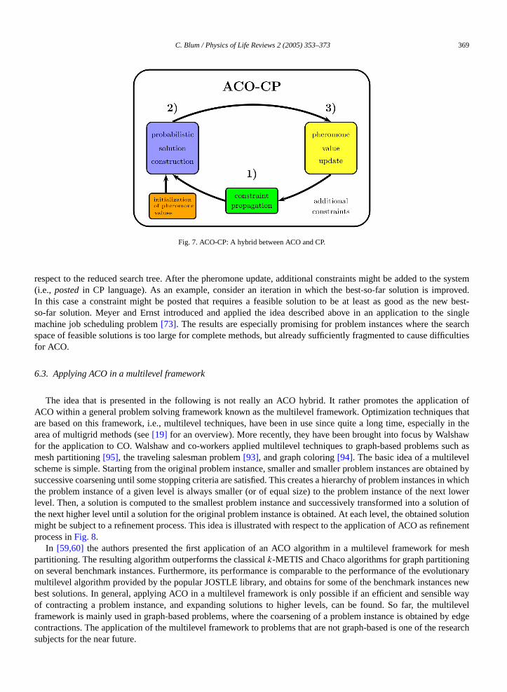
The idea of hybridizing ACO with CP is graphically shown inFig. 7. At each iteration, first constraint propagatiis applied in order to reduce the remaining search tree. Then, solutions are constructed in the standard ACO

8 Note that an inaccurate lower bound might bias the search towards bad areas of the search space.


he systemroved.

new best-e singleearch

ifficulties

tion ofes thatlly in thehawsuch asltained bys in whichxt lowerlution ofolution

finement

meshngolutionaryes newle wayultilevelby edge

research

Fig. 7. ACO-CP: A hybrid between ACO and CP.

respect to the reduced search tree. After the pheromone update, additional constraints might be added to t(i.e., postedin CP language). As an example, consider an iteration in which the best-so-far solution is impIn this case a constraint might be posted that requires a feasible solution to be at least as good as theso-far solution. Meyer and Ernst introduced and applied the idea described above in an application to thmachine job scheduling problem[73]. The results are especially promising for problem instances where the sspace of feasible solutions is too large for complete methods, but already sufficiently fragmented to cause dfor ACO.

6.3. Applying ACO in a multilevel framework

The idea that is presented in the following is not really an ACO hybrid. It rather promotes the applicaACO within a general problem solving framework known as the multilevel framework. Optimization techniquare based on this framework, i.e., multilevel techniques, have been in use since quite a long time, especiaarea of multigrid methods (see[19] for an overview). More recently, they have been brought into focus by Walsfor the application to CO. Walshaw and co-workers applied multilevel techniques to graph-based problemsmesh partitioning[95], the traveling salesman problem[93], and graph coloring[94]. The basic idea of a multilevescheme is simple. Starting from the original problem instance, smaller and smaller problem instances are obsuccessive coarsening until some stopping criteria are satisfied. This creates a hierarchy of problem instancethe problem instance of a given level is always smaller (or of equal size) to the problem instance of the nelevel. Then, a solution is computed to the smallest problem instance and successively transformed into a sothe next higher level until a solution for the original problem instance is obtained. At each level, the obtained smight be subject to a refinement process. This idea is illustrated with respect to the application of ACO as reprocess inFig. 8.

In [59,60] the authors presented the first application of an ACO algorithm in a multilevel framework forpartitioning. The resulting algorithm outperforms the classicalk-METIS and Chaco algorithms for graph partitionion several benchmark instances. Furthermore, its performance is comparable to the performance of the evmultilevel algorithm provided by the popular JOSTLE library, and obtains for some of the benchmark instancbest solutions. In general, applying ACO in a multilevel framework is only possible if an efficient and sensibof contracting a problem instance, and expanding solutions to higher levels, can be found. So far, the mframework is mainly used in graph-based problems, where the coarsening of a problem instance is obtainedcontractions. The application of the multilevel framework to problems that are not graph-based is one of thesubjects for the near future.


cean be

d

imizationunctionechniquethan theobjects

eue

searchr findingCOon the

utlinedts today.lined thevided a

al artifi-earch andpace thated. Otherpplica-ibilities

Fig. 8. ML-ACO: Applying ACO in the multilevel framework. The original problem instance isP . In an iterative process this problem instanis simplified (i.e., contracted) until the lowest level instancePn is reached. Then, an ACO algorithm (or any other optimization technique) c

used to tackle problemPn. The obtained best solutionsn is expanded into a solutionsn−1′of the next bigger problem instancePn−1. With this

solution as the first best-so-far solution, the same ACO algorithm might be applied to tackle problem instancePn−1 resulting in a best obtainesolutionsn−1. This process goes on until the original problem instance was tackled.

6.4. Applying ACO to an auxiliary search space

The idea that we present in this section is based on replacing the original search space of the tackled optproblem with an auxiliary search space to which ACO is then applied. A precondition for this technique is a fthat maps each object from the auxiliary search space to a solution to the tackled optimization problem. This tcan be beneficial in case (1) the generation of objects from the auxiliary search space is more efficientconstruction of solutions to the optimization problem at hand, and/or (2) the mapping function is such thatfrom the auxiliary search space are mapped to high quality solutions of the original search space.

An example of such a hybrid ACO algorithm was presented in[10] for the application to thek-cardinality tree(KCT) problem. In this problem is given an edge-weighted graph and a cardinalityk > 0. The original search spacconsists of all trees in the given graph with exactlyk edges, i.e., allk-cardinality trees. The objective function valof a given tree is computed as the sum of the weights of its edges. The authors of[10] chose the set of alll-cardinalitytrees (wherel > k, andl fixed) in the given graph as auxiliary search space. The mapping between the auxiliaryspace and the original search space was performed by a polynomial-time dynamic programming algorithm fothe optimalk-cardinality tree that is contained in anl-cardinality tree. The experimental results show that the Aalgorithm working on the auxiliary search space significantly improves over the same ACO algorithm workingoriginal search space.

7. Conclusions

In this work we first gave a detailed description of the origins and the basics of ACO algorithms. Then we othe general framework of the ACO metaheuristic and presented some of the most successful ACO varianAfter listing some representative applications of ACO, we summarized the existing theoretical results and outlatest developments concerning the adaptation of ACO algorithms to continuous optimization. Finally, we prosurvey on a very interesting recent research direction: The hybridization of ACO algorithms with more classiccial intelligence and operations research methods. As examples we presented the hybridization with beam swith constraint programming. The central idea behind these two approaches is the reduction of the search shas to be explored by ACO. This can be especially useful when large scale problem instances are considerhybridization examples are the application of ACO for solution refinement in multilevel frameworks, and the ation of ACO to auxiliary search spaces. In the opinion of the author, this research direction offers many possfor valuable future research.


I) Syst

ceedings

relo JJ,erence on

the AISB

s. Antr; 2002.

ne DW,comput-

erlags-

Opera-

J,inspired

72.Comput

3):268–

5–308.roceed-

99.

ons, and, vol. 110.

lutionary

tions Res

Behavior

problems.

olph G,ing from

90;3:159–

–65.portfolio

[in Ital

Acknowledgements

Many thanks to the anonymous referees for helping immensely to improve this paper.

References

[1] Alupoaei S, Katkoori S. Ant colony system application to marcocell overlap removal. IEEE Trans Very Large Scale Integr (VLS2004;12(10):1118–22.

[2] Bautista J, Pereira J. Ant algorithms for assembly line balancing. In: Dorigo M, Di Caro G, Sampels M, editors. Ant algorithms—Proof ANTS 2002—Third international workshop. Lecture Notes in Comput Sci, vol. 2463. Berlin: Springer; 2002. p. 65–75.

[3] Bertsekas DP, Tsitsiklis JN, Wu C. Rollout algorithms for combinatorial optimization. J Heuristics 1997;3:245–62.[4] Bianchi L, Gambardella LM, Dorigo M. An ant colony optimization approach to the probabilistic traveling salesman problem. In: Me

Adamidis P, Beyer H-G, Fernández-Villacanas J-L, Schwefel H-P, editors. Proceedings of PPSN-VII, seventh international confparallel problem solving from nature. Lecture Notes in Comput Sci, vol. 2439. Berlin: Springer; 2002. p. 883–92.

[5] Bilchev B, Parmee IC. The ant colony metaphor for searching continuous design spaces. In: Fogarty TC, editor. Proceedings ofworkshop on evolutionary computation. Lecture Notes in Comput Sci, vol. 993. Berlin: Springer; 1995. p. 25–39.

[6] Birattari M, Di Caro G, Dorigo M. Toward the formal foundation of ant programming. In: Dorigo M, Di Caro G, Sampels M, editoralgorithms—Proceedings of ANTS 2002—Third international workshop. Lecture Notes in Comput Sci, vol. 2463. Berlin: Springep. 188–201.

[7] Blesa M, Blum C. Ant colony optimization for the maximum edge-disjoint paths problem. In: Raidl GR, Cagnoni S, Branke J, CorDrechsler R, Jin Y, Johnson CG, Machado P, Marchiori E, Rothlauf R, Smith GD, Squillero G, editors. Applications of evolutionarying, proceedings of EvoWorkshops 2004. Lecture Notes in Comput Sci, vol. 3005. Berlin: Springer; 2004. p. 160–9.

[8] Blum C. Theoretical and practical aspects of Ant colony optimization. Dissertations in Artificial Intelligence. Berlin: Akademische Vgesellschaft Aka GmbH; 2004.

[9] Blum C. Beam-ACO—Hybridizing ant colony optimization with beam search: An application to open shop scheduling. Computers &tions Res 2005;32(6):1565–91.

[10] Blum C, Blesa MJ. Combining ant colony optimization with dynamic programming for solving thek-cardinality tree problem. In: CabestanyPrieto A, Sandoval F, editors. 8th international work-conference on artificial neural networks, computational intelligence and biosystems (IWANN’05). Lecture Notes in Comput Sci, vol. 3512. Berlin: Springer; 2005. p. 25–33.

[11] Blum C, Dorigo M. The hyper-cube framework for ant colony optimization. IEEE Trans Syst Man Cybernet Part B 2004;34(2):1161–[12] Blum C, Dorigo M. Search bias in ant colony optimization: On the role of competition-balanced systems. IEEE Trans Evolutionary

2005;9(2):159–74.[13] Blum C, Roli A. Metaheuristics in combinatorial optimization: Overview and conceptual comparison. ACM Comput Surveys 2003;35(

308.[14] Blum C, Sampels M. An ant colony optimization algorithm for shop scheduling problems. J Math Modelling Algorithms 2004;3(3):28[15] Blum C, Socha K. Training feed-forward neural networks with ant colony optimization: An application to pattern classification. In: P

ings of the 5th international conference on hybrid intelligent systems (HIS). Piscataway, NJ: IEEE Press; 2005. p. 233–8.[16] Bonabeau E, Dorigo M, Theraulaz G. Swarm intelligence: From natural to artificial systems. New York: Oxford University Press; 19[17] Bonabeau E, Dorigo M, Theraulaz G. Inspiration for optimization from social insect behavior. Nature 2000;406:39–42.[18] Box GEP, Muller ME. A note on the generation of random normal deviates. Ann Math Statist 1958;29(2):610–1.[19] Brandt A. Multilevel computations: Review and recent developments. In: McCormick SF, editor. Multigrid methods: Theory, applicati

supercomputing, proceedings of the 3rd Copper Mountain conference on multigrid methods. Lecture Notes in Pure and Appl MathNew York: Marcel Dekker; 1988. p. 35–62.

[20] Bui TN, Rizzo JR. Finding maximum cliques with distributed ants. In: Deb K, et al., editors. Proceedings of the genetic and evocomputation conference (GECCO 2004). Lecture Notes in Comput Sci, vol. 3102. Berlin: Springer; 2004. p. 24–35.

[21] Bullnheimer B, Hartl R, Strauss C. A new rank-based version of the Ant System: A computational study. Central European J OperaEconom 1999;7(1):25–38.

[22] Campos M, Bonabeau E, Theraulaz G, Deneubourg J-L. Dynamic scheduling and division of labor in social insects. Adapt2000;8(3):83–96.

[23] Corry P, Kozan E. Ant colony optimisation for machine layout problems. Comput Optim Appl 2004;28(3):287–310.[24] Costa D, Hertz A. Ants can color graphs. J Oper Res Soc 1997;48:295–305.[25] Della Croce F, Ghirardi M, Tadei R, Recovering beam search: enhancing the beam search approach for combinatorial optimisation

In: Proceedings of PLANSIG 2002—21th workshop of the UK planning and scheduling special interest group; 2002. p. 149–69.[26] den Besten ML, Stützle T, Dorigo M. Ant colony optimization for the total weighted tardiness problem. In: Schoenauer M, Deb K, Rud

Yao X, Lutton E, Merelo JJ, Schwefel H-P, editors. Proceedings of PPSN-VI, sixth international conference on parallel problem solvnature. Lecture Notes in Comput Sci, vol. 1917. Berlin: Springer; 2000. p. 611–20.

[27] Deneubourg J-L, Aron S, Goss S, Pasteels J-M. The self-organizing exploratory pattern of the Argentine ant. J Insect Behaviour 1968.

[28] Di Caro G, Dorigo M. AntNet: Distributed stigmergetic control for communications networks. J Artificial Intelligence Res 1998;9:317[29] Doerner K, Gutjahr WJ, Hartl RF, Strauss C, Stummer C. Pareto ant colony optimization: A metaheuristic approach to multiobjective

selection. Ann Oper Res 2004;131:79–99.[30] Dorigo M, Optimization, learning and natural algorithms. PhD thesis, Dipartimento di Elettronica, Politecnico di Milano, Italy, 1992-

ian].


lutionary

litecnico

t Part B

tions. In:otes in

tworks

equence-

editors.. p. 622–7.Comput

dows.

m C,ization

blems. In:idl GR,. Berlin:

éorie de

tzle T,Notes in

ttlieb J,Work-

itzler E,2003).

edicine

rks, vol. 4.

LM,intelli-

attari M,ny opti-

the third501–8.

[31] Dorigo M, Blum C. Ant colony optimization theory: A survey. Theoret Comput Sci 2005;344(2–3):243–78.[32] Dorigo M, Di Caro G, Gambardella LM. Ant algorithms for discrete optimization. Artificial Life 1999;5(2):137–72.[33] Dorigo M, Gambardella LM. Ant colony system: A cooperative learning approach to the traveling salesman problem. IEEE Trans Evo

Comput 1997;1(1):53–66.[34] Dorigo M, Maniezzo V, Colorni A, Positive feedback as a search strategy. Technical Report 91-016, Dipartimento di Elettronica, Po

di Milano, Italy, 1991.[35] Dorigo M, Maniezzo V, Colorni A. Ant System: Optimization by a colony of cooperating agents. IEEE Trans Syst Man Cyberne

1996;26(1):29–41.[36] Dorigo M, Stützle T. Ant Colony optimization. Cambridge, MA: MIT Press; 2004.[37] Dréo J, Siarry P. A new ant colony algorithm using the heterarchical concept aimed at optimization of multiminima continuous func

Dorigo M, Di Caro G, Sampels M, editors. Ant algorithms—Proceedings of ANTS 2002—Third international workshop. Lecture NComput Sci, vol. 2463. Berlin: Springer; 2002. p. 216–21.

[38] Duin C, Voß S. The pilot method: A strategy for heuristic repetition with application to the steiner problem in graphs. Ne1999;34(3):181–91.

[39] Gagné C, Price WL, Gravel M. Comparing an ACO algorithm with other heuristics for the single machine scheduling problem with sdependent setup times. J Oper Res Soc 2002;53:895–906.

[40] Gambardella LM, Dorigo M. Solving symmetric and asymmetric TSPs by ant colonies. In: Baeck T, Fukuda T, Michalewicz Z,Proceedings of the 1996 IEEE international conference on evolutionary computation (ICEC’96). Piscataway, NJ: IEEE Press; 1996

[41] Gambardella LM, Dorigo M. Ant Colony System hybridized with a new local search for the sequential ordering problem. INFORMS J2000;12(3):237–55.

[42] Gambardella LM, Taillard ÉD, Agazzi G. MACS-VRPTW: A multiple ant colony system for vehicle routing problems with time winIn: Corne D, Dorigo M, Glover F, editors. New ideas in optimization. London: McGraw-Hill; 1999. p. 63–76.

[43] Gandibleux X, Delorme X, T’Kindt V. An ant colony optimisation algorithm for the set packing problem. In: Dorigo M, Birattari M, BluGambardella LM, Mondada F, Stützle T, editors. Proceedings of ANTS 2004—Fourth international workshop on Ant colony optimand swarm intelligence. Lecture Notes in Comput Sci, vol. 3172. Berlin: Springer; 2004. p. 49–60.

[44] Garey MR, Johnson DS. Computers and intractability; A guide to the theory of NP Completeness. New York: WH Freeman; 1979.[45] Ginsberg ML. Essentials of artificial intelligence. San Mateo, CA: Morgan Kaufmann; 1993.[46] Glover F. Future paths for integer programming and links to artificial intelligence. Comput Oper Res 1986;13:533–49.[47] Glover F, Kochenberger G, editors. Handbook of metaheuristics. Norwell, MA: Kluwer Academic; 2002.[48] Gottlieb J, Puchta M, Solnon C. A study of greedy, local search, and ant colony optimization approaches for car sequencing pro

Cagnoni S, Romero Cardalda JJ, Corne DW, Gottlieb J, Guillot A, Hart E, Johnson CG, Marchiori E, Meyer J-A, Middendorf M, Raeditors. Applications of evolutionary computing, proceedings of EvoWorkshops, 2003. Lecture Notes in Comput Sci, vol. 2611Springer; 2003. p. 246–57.

[49] Grassé P-P. La reconstruction du nid et les coordinations inter-individuelles chez bellicositermes natalensis et cubitermes sp. La thlastigmergie: Essai d’interprétation des termites constructeurs. Insectes Sociaux 1959;6:41–81.

[50] Guéret C, Monmarché N, Slimane M. Ants can play music. In: Dorigo M, Birattari M, Blum C, Gambardella LM, Mondada F, Stüeditors. Proceedings of ANTS 2004—Fourth international workshop on Ant colony optimization and swarm intelligence. LectureComput Sci, vol. 3172. Berlin: Springer; 2004. p. 310–7.

[51] Guntsch M, Middendorf M. Pheromone modification strategies for ant algorithms applied to dynamic TSP. In: Boers EJW, GoLanzi PL, Smith RE, Cagnoni S, Hart E, Raidl GR, Tijink H, editors. Applications of evolutionary computing: Proceedings of Evoshops, 2001. Lecture Notes in Comput Sci, vol. 2037. Berlin: Springer; 2001. p. 213–22.

[52] Guntsch M, Middendorf M. Solving multi-objective permutation problems with population based ACO. In: Fonseca CM, Fleming PJ, ZDeb K, Thiele L, editors. Proceedings of the second international conference on evolutionary multi-criterion optimization (EMOLecture Notes in Comput Sci, vol. 2636. Berlin: Springer; 2003. p. 464–78.

[53] Gutjahr WJ. A graph-based ant system and its convergence. Future Generat Comput Syst 2000;16(9):873–88.[54] Gutjahr WJ. ACO algorithms with guaranteed convergence to the optimal solution. Informat Process Lett 2002;82(3):145–53.[55] Handl J, Knowles J, Dorigo M. Ant-based clustering and topographic mapping. Artificial Life 2006;12(1). In press.[56] Hoos HH, Stützle T. Stochastic local search: Foundations and applications. Amsterdam: Elsevier; 2004.[57] Karpenko O, Shi J, Dai Y. Prediction of MHC class II binders using the ant colony search strategy. Artificial Intelligence in M

2005;35(1–2):147–56.[58] Kennedy J, Eberhart RC. Particle swarm optimization. In: Proceedings of the 1995 IEEE international conference on neural netwo

Piscataway, NJ: IEEE Press; 1995. p. 1942–8.[59] Korošec P, Šilc J, Robic B. Mesh-partitioning with the multiple ant-colony algorithm. In: Dorigo M, Birattari M, Blum C, Gambardella

Mondada F, Stützle T, editors. Proceedings of ANTS 2004—Fourth international workshop on Ant colony optimization and swarmgence. Lecture Notes in Comput Sci, vol. 3172. Berlin: Springer; 2004. p. 430–1.

[60] Korošec P, Šilc J, Robic B. Solving the mesh-partitioning problem with an ant-colony algorithm. Parallel Comput 2004;30:785–801.[61] Lawler E, Lenstra JK, Rinnooy Kan AHG, Shmoys DB. The travelling Salesman problem. New York: John Wiley & Sons; 1985.[62] López-Ibáñez M, Paquete L, Stützle T. On the design of ACO for the biobjective quadratic assignment problem. In: Dorigo M, Bir

Blum C, Gambardella LM, Mondada F, Stützle T, editors. Proceedings of ANTS 2004—Fourth international workshop on Ant colomization and swarm intelligence. Lecture Notes in Comput Sci, vol. 3172. Berlin: Springer; 2004. p. 214–25.

[63] Lumer E, Faieta B. Diversity and adaptation in populations of clustering ants. In: Meyer J-A, Wilson SW, editors. Proceedings ofinternational conference on simulation of adaptive behavior: From animals to animats, vol. 3. Cambridge, MA: MIT Press; 1994. p.


J Comput

lla LM,intelli-

(5):769–

rs. Antr; 2002.

hms—62.

Comput

tzle T,Notes in

, Bäck T,e. Lecture

mput Syst

echt RF,

omput

er Res

rigo M,put Sci,

Bioin-

ors. Antr; 2002.

tzle T,Notes in

-art. In:GR, ed-pringer;

computing

.

ol

r Res

[64] Maniezzo V. Exact and approximate nondeterministic tree-search procedures for the quadratic assignment problem. INFORMS1999;11(4):358–69.

[65] Maniezzo V, Boschetti M, Jelasity M. An ant approach to membership overlay design. In: Dorigo M, Birattari M, Blum C, GambardeMondada F, Stützle T, editors. Proceedings of ANTS 2004—Fourth international workshop on Ant colony optimization and swarmgence. Lecture Notes in Comput Sci, vol. 3172. Berlin: Springer; 2004. p. 37–48.

[66] Maniezzo V, Colorni A. The Ant System applied to the quadratic assignment problem. IEEE Trans Data Knowledge Engrg 1999;1178.

[67] Maniezzo V, Milandri M. An ant-based framework for very strongly constrained problems. In: Dorigo M, Di Caro G, Sampels M, editoalgorithms—Proceedings of ANTS 2002—Third international workshop. Lecture Notes in Comput Sci, vol. 2463. Berlin: Springep. 222–7.

[68] Marriott K, Stuckey P. Programming with constraints. Cambridge, MA: MIT Press; 1998.[69] Merkle D, Middendorf M. Modelling ACO: Composed permutation problems. In: Dorigo M, Di Caro G, Sampels M, editors. Ant algorit

Proceedings of ANTS 2002—Third international workshop. Lecture Notes in Comput Sci, vol. 2463. Berlin: Springer; 2002. p. 149–[70] Merkle D, Middendorf M. Modelling the dynamics of ant colony optimization algorithms. Evolutionary Comput 2002;10(3):235–62.[71] Merkle D, Middendorf M, Schmeck H. Ant colony optimization for resource-constrained project scheduling. IEEE Trans Evolutionary

2002;6(4):333–46.[72] Meuleau N, Dorigo M. Ant colony optimization and stochastic gradient descent. Artificial Life 2002;8(2):103–21.[73] Meyer B, Ernst A. Integrating ACO and constraint propagation. In: Dorigo M, Birattari M, Blum C, Gambardella LM, Mondada F, Stü

editors. Proceedings of ANTS 2004—Fourth international workshop on Ant colony optimization and swarm intelligence. LectureComput Sci, vol. 3172. Berlin: Springer; 2004. p. 166–77.

[74] Michel R, Middendorf M. An island model based ant system with lookahead for the shortest supersequence problem. In: Eiben AESchoenauer M, Schwefel H-P, editors. Proceedings of PPSN-V, fifth international conference on parallel problem solving from naturNotes in Comput Sci, vol. 1498. Berlin: Springer; 1998. p. 692–701.

[75] Monmarché N, Venturini G, Slimane M. On how pachycondyla apicalis ants suggest a new search algorithm. Future Generation Co2000;16:937–46.

[76] Moss JD, Johnson CG. An ant colony algorithm for multiple sequence alignment in bioinformatics. In: Pearson DW, Steele NC, Albreditors. Artificial neural networks and genetic algorithms. Berlin: Springer; 2003. p. 182–6.

[77] Nemhauser GL, Wolsey AL. Integer and combinatorial optimization. New York: John Wiley & Sons; 1988.[78] Ow PS, Morton TE. Filtered beam search in scheduling. Internat J Production Res 1988;26:297–307.[79] Papadimitriou CH, Steiglitz K. Combinatorial optimization—Algorithms and complexity. New York: Dover; 1982.[80] Parpinelli RS, Lopes HS, Freitas AA. Data mining with an ant colony optimization algorithm. IEEE Trans Evolutionary C

2002;6(4):321–32.[81] Reeves CR, editor. Modern heuristic techniques for combinatorial problems. New York: John Wiley & Sons; 1993.[82] Reimann M, Doerner K, Hartl RF.D-ants: Savings based ants divide and conquer the vehicle routing problems. Comput Op

2004;31(4):563–91.[83] Shmygelska A, Aguirre-Hernández R, Hoos HH. An ant colony optimization algorithm for the 2D HP protein folding problem. In: Do

Di Caro G, Sampels M, editors. Ant algorithms—Proceedings of ANTS 2002—Third international workshop. Lecture Notes in Comvol. 2463. Berlin: Springer; 2002. p. 40–52.

[84] Shmygelska A, Hoos HH. An ant colony optimisation algorithm for the 2D and 3D hydrophobic polar protein folding problem. BMCformatics 2005;6(30):1–22.

[85] Silva CA, Runkler TA, Sousa JM, Palm R. Ant colonies as logistic processes optimizers. In: Dorigo M, Di Caro G, Sampels M, editalgorithms—Proceedings of ANTS 2002—Third international workshop. Lecture Notes in Comput Sci, vol. 2463. Berlin: Springep. 76–87.

[86] Socha K. ACO for continuous and mixed-variable optimization. In: Dorigo M, Birattari M, Blum C, Gambardella LM, Mondada F, Stüeditors. Proceedings of ANTS 2004—Fourth international workshop on Ant colony optimization and swarm intelligence. LectureComput Sci, vol. 3172. Berlin: Springer; 2004. p. 25–36.

[87] Socha K, Sampels M, Manfrin M. Ant algorithms for the university course timetabling problem with regard to the state-of-theCagnoni S, Romero Cardalda JJ, Corne DW, Gottlieb J, Guillot A, Hart E, Johnson CG, Marchiori E, Meyer A, Middendorf M, Raidlitors. Applications of evolutionary computing, proceedings of EvoWorkshops 2003. Lecture Notes in Comput Sci, vol. 2611. Berlin: S2003. p. 334–45.

[88] Solnon C. Ant can solve constraint satisfaction problems. IEEE Trans Evolutionary Comput 2002;6(4):347–57.[89] Stützle T. An ant approach to the flow shop problem. In: Proceedings of the 6th european congress on intelligent techniques & soft

(EUFIT’98). Aachen: Verlag Mainz; 1998. p. 1560–4.[90] Stützle T, Dorigo M. A short convergence proof for a class of ACO algorithms. IEEE Trans Evolutionary Comput 2002;6(4):358–65[91] Stützle T, Hoos HH.MAX–MIN Ant system. Future Generat Comput Syst 2000;16(8):889–914.[92] Unger R, Moult J. Finding the lowest free-energy conformation of a protein is anNP -hard problem: Proofs and implications. Bull Math Bi

1993;55(6):1183–98.[93] Walshaw C. A multilevel approach to the travelling salesman problem. Oper Res 2002;50(5):862–77.[94] Walshaw C. Multilevel refinement for combinatorial optimization problems. Ann Oper Res 2004;131:325–72.[95] Walshaw C, Cross M. Mesh partitioning: A multilevel balancing and refinement algorithm. SIAM J Sci Comput 2000;22(1):63–80.[96] Zlochin M, Birattari M, Meuleau N, Dorigo M. Model-based search for combinatorial optimization: A critical survey. Ann Ope

2004;131(1–4):373–95.

Ant colony optimization: Introduction and recent trends

Documents

Transcript of Ant colony optimization: Introduction and recent trends