Ant Colony Optimization: An Alternative Heuristic for ...

Ant Colony Optimization: An Alternative Heuristic for Aerospace DesignApplications

by

Zachary John Kiyak

A thesis submitted to the Graduate Faculty ofAuburn University

in partial fulfillment of therequirements for the Degree of

Master of Science

Auburn, AlabamaMay 04, 2014

Keywords: optimization, solid rocket motor, missile design, ant colony algorithm

Copyright 2014 by Zachary John Kiyak

Approved by

Roy Hartfield, Chair, Walt and Virginia Waltosz Professor of Aerospace EngineeringBrian Thurow, Professor of Aerospace Engineering

Andrew Shelton, Professor of Aerospace Engineering

Abstract

A modified ant colony optimization (ACO) algorithm is applied to a set of solid-rocket-

motor and single-stage solid missile design problems. A local search procedure is also in-

tegrated with the algorithm, adding a search intensification ability that compliments the

ability of ACO to thoroughly explore a solution space. The goal of this work is to evaluate

the effectiveness of the ant colony optimization scheme by comparing its solution output

quality with those of other, well-known optimization methods. Performance is based on

solution “fitness”, or how closely each solution matches a specific set of performance objec-

tives, as well as the number of calls to the objective function that are required in order to

reach that solution. Additionally, an important performance criterion is to determine the

algorithm′s capabilities of finding, not only a single quality solution to a design problem, but

also a diverse set of additional, near-optimal solutions.

ii

Acknowledgments

Special thanks to Dr. John Burkhalter for his help with the FORTRAN coding, Dr.

Roy Hartfield for his direction, and Timothy Ledlow for his help in interpreting the missile

trajectory program.

Also, I would like to thank my parents for their support and financial understanding

over the years.

iii

Table of Contents

Abstract . . . . . . . . . . . . . . . . . . . . . . . . . . . . . . . . . . . . . . . . . . . ii

Acknowledgments . . . . . . . . . . . . . . . . . . . . . . . . . . . . . . . . . . . . . . iii

List of Figures . . . . . . . . . . . . . . . . . . . . . . . . . . . . . . . . . . . . . . . vi

List of Tables . . . . . . . . . . . . . . . . . . . . . . . . . . . . . . . . . . . . . . . . viii

Nomenclature . . . . . . . . . . . . . . . . . . . . . . . . . . . . . . . . . . . . . . . . ix

1 Introduction . . . . . . . . . . . . . . . . . . . . . . . . . . . . . . . . . . . . . . 1

2 Overview of Ant Colony Optimization . . . . . . . . . . . . . . . . . . . . . . . 2

2.1 Natural Inspiration . . . . . . . . . . . . . . . . . . . . . . . . . . . . . . . . 2

2.2 Artificial Algorithm . . . . . . . . . . . . . . . . . . . . . . . . . . . . . . . . 3

2.3 Modifications . . . . . . . . . . . . . . . . . . . . . . . . . . . . . . . . . . . 8

3 Overview of Competing Algorithms and Complimentary Local Search Methods . 12

3.1 Genetic Algorithm and Particle Swarm Methodology . . . . . . . . . . . . . 12

3.2 Direct Local Search Methods . . . . . . . . . . . . . . . . . . . . . . . . . . . 13

3.2.1 Pattern Search . . . . . . . . . . . . . . . . . . . . . . . . . . . . . . 13

3.2.2 Nelder-Mead Simplex . . . . . . . . . . . . . . . . . . . . . . . . . . . 14

4 Star-Grain Solid Rocket Motor Design Optimization . . . . . . . . . . . . . . . . 17

4.1 Solid Rocket Motor System Background . . . . . . . . . . . . . . . . . . . . 17

4.2 Optimization Procedure . . . . . . . . . . . . . . . . . . . . . . . . . . . . . 17

4.3 SRM Curve Matching Problems and Results . . . . . . . . . . . . . . . . . . 20

5 Solid Motor Sounding Rocket Optimization . . . . . . . . . . . . . . . . . . . . 26

5.1 Sounding Rocket System Description . . . . . . . . . . . . . . . . . . . . . . 26

5.2 Sounding Rocket Results . . . . . . . . . . . . . . . . . . . . . . . . . . . . . 27

6 Description of 6DOF Missile System . . . . . . . . . . . . . . . . . . . . . . . . 32

iv

7 Single Stage Solid Missile System Optimizer Comparisons . . . . . . . . . . . . 36

7.1 Match Range - 250,000 ft . . . . . . . . . . . . . . . . . . . . . . . . . . . . . 36

7.2 Match Range - 750,000 ft . . . . . . . . . . . . . . . . . . . . . . . . . . . . . 38

7.3 Match a Single Trajectory . . . . . . . . . . . . . . . . . . . . . . . . . . . . 42

7.4 Match Three Trajectories . . . . . . . . . . . . . . . . . . . . . . . . . . . . . 43

8 Local Search Testing . . . . . . . . . . . . . . . . . . . . . . . . . . . . . . . . . 54

9 Summary and Recommendations . . . . . . . . . . . . . . . . . . . . . . . . . . 57

Bibliography . . . . . . . . . . . . . . . . . . . . . . . . . . . . . . . . . . . . . . . . 59

Appendices . . . . . . . . . . . . . . . . . . . . . . . . . . . . . . . . . . . . . . . . . 63

Appendix A: Solid Rocket Design Limits and Parameter Settings . . . . . . . . . . . 64

Appendix B: Sounding Rocket Optimizer Input File . . . . . . . . . . . . . . . . . . . 65

Appendix C: Sounding Rocket Constants and Goals Input File . . . . . . . . . . . . 66

Appendix D: Single-Stage Rocket Input File for Range Matching Problems . . . . . . 67

Appendix E: Design Constraints for Trajectory Matching Problems . . . . . . . . . . 68

Modified ACO Algorithm Source Code Information . . . . . . . . . . . . . . . . . . . 69

v

List of Figures

2.1 Double Bridge Experiment [18] . . . . . . . . . . . . . . . . . . . . . . . . . . . 3

2.2 Probability Density Function . . . . . . . . . . . . . . . . . . . . . . . . . . . . 5

2.3 Gaussian Kernel Construction . . . . . . . . . . . . . . . . . . . . . . . . . . . . 5

2.4 Simple 1-D Illustration of Single Ant Cycle . . . . . . . . . . . . . . . . . . . . 7

2.5 ACO-R Algorithm Flow . . . . . . . . . . . . . . . . . . . . . . . . . . . . . . . 9

2.6 Effects of parameter “q” on PDF selection . . . . . . . . . . . . . . . . . . . . . 10

2.7 Effects of parameter “qmod” on PDF selection . . . . . . . . . . . . . . . . . . . 10

3.1 Hooke and Jeeves Pattern Search [37] . . . . . . . . . . . . . . . . . . . . . . . . 14

3.2 2-D Simplex Morphology . . . . . . . . . . . . . . . . . . . . . . . . . . . . . . . 15

4.1 Star Grain Cross Sectional Geometry [40] . . . . . . . . . . . . . . . . . . . . . 18

4.2 Optimized SRM Grain Geometry - Random Burn . . . . . . . . . . . . . . . . . 21

4.3 Chamber Pressure vs Time Curve - Random Burn Profile . . . . . . . . . . . . 21

4.4 Chamber Pressure vs Time Match - Neutral Burn Profile . . . . . . . . . . . . . 22

4.5 Optimized SRM Grain Geometry - Neutral Burn . . . . . . . . . . . . . . . . . 22

4.6 Thrust vs Time Curve - Regressive-Progressive Burn . . . . . . . . . . . . . . . 24

vi

4.7 Optimized SRM Grain Geometry - Regressive Progressive . . . . . . . . . . . . 24

5.1 Best Sounding Rocket Solutions Found by Optimizers . . . . . . . . . . . . . . . 28

5.2 Optimizer Convergence History . . . . . . . . . . . . . . . . . . . . . . . . . . . 29

5.3 Example Alternate Sounding Rocket Solutions . . . . . . . . . . . . . . . . . . . 31

6.1 Single Stage Solid Missile System . . . . . . . . . . . . . . . . . . . . . . . . . . 33

7.1 Convergence History - Match 250,000 ft . . . . . . . . . . . . . . . . . . . . . . 37

7.2 Example Alternate Sounding Rocket Solutions - 250,000 ft . . . . . . . . . . . . 39

7.3 Convergence History - Match 750,000 ft . . . . . . . . . . . . . . . . . . . . . . 40

7.4 Example Alternate Sounding Rocket Solutions - 750,000 ft . . . . . . . . . . . . 41

7.5 Single Trajectory Convergence History . . . . . . . . . . . . . . . . . . . . . . . 43

7.6 3-D Optimized Missile Design - 164 km trajectory . . . . . . . . . . . . . . . . . 45

7.7 Optimized Missiles - 164km Trajectory . . . . . . . . . . . . . . . . . . . . . . . 46

7.8 Optimized Trajectory Match - 164 km . . . . . . . . . . . . . . . . . . . . . . . 47

7.9 Three-Trajectory Convergence History . . . . . . . . . . . . . . . . . . . . . . . 50

7.10 Optimized Missiles - Three Trajectories . . . . . . . . . . . . . . . . . . . . . . 51

7.11 3-D Optimized Missile Design - Three Trajectories . . . . . . . . . . . . . . . . 52

7.12 Optimized Three-Trajectory Matches . . . . . . . . . . . . . . . . . . . . . . . . 53

vii

List of Tables

4.1 SRM Optimization Design Parameters . . . . . . . . . . . . . . . . . . . . . . . 19

4.2 Local Search Performance Comparison . . . . . . . . . . . . . . . . . . . . . . . 20

4.3 Summary of Results and Optimized SRM Geometries . . . . . . . . . . . . . . . 25

5.1 Sounding Rocket Design Parameters . . . . . . . . . . . . . . . . . . . . . . . . 27

5.2 Sounding Rocket Optimization Results . . . . . . . . . . . . . . . . . . . . . . . 30

5.3 Sounding Rocket Multiple Solutions . . . . . . . . . . . . . . . . . . . . . . . . 30

6.1 List of Single Stage Solid Missile Design Variables . . . . . . . . . . . . . . . . . 34

6.2 Classification of Initial Missile Design Code Constants . . . . . . . . . . . . . . 35

7.1 Results for Range Matching Problem - 250,000 ft . . . . . . . . . . . . . . . . . 37

7.2 Results for Range Matching Problem - 750,000 ft . . . . . . . . . . . . . . . . . 40

7.3 Single Trajectory Results . . . . . . . . . . . . . . . . . . . . . . . . . . . . . . 44

7.4 Multiple Alternate Solutions - 164 km Trajectory . . . . . . . . . . . . . . . . . 48

7.5 Three Trajectory Results . . . . . . . . . . . . . . . . . . . . . . . . . . . . . . . 49

7.6 Multiple Alternate Solutions - Three Trajectory Problem . . . . . . . . . . . . . 50

8.1 Local Search Improvements - 164km Trajectory . . . . . . . . . . . . . . . . . . 54



8.4 Local Search Improvements - Three Trajectories . . . . . . . . . . . . . . . . . . 55

1 Variable Ranges Used for SRM Curve Matching Problems . . . . . . . . . . . . 64

2 Algorithm Parameters Used for SRM Curve Matching Problems . . . . . . . . . 64

viii

Nomenclature

ζ Pheromone Evaporation Rate

ACO Ant Colony Optimization

GA Genetic Algorithm

gl Propellant Grain Length

j Solution Archive Index

k Solution Archive Size

kfuel Propellant Fuel Type

NSP Number of Star Points

PDF Probability Density Function

PSO Particle Swarm Optimization

ptang Star Point Angle

q Pheromone Weight Distribution Parameter

qmod ACO Elitism Parameter

ratio Nozzle Expansion Ratio

rbi Outer Grain Radius

ri Propellant Inner Grain Radius

RMSE Root Mean Square Error

ix

rp Propellant Outer Grain Radius

RPSO Repulsive Particle Swarm Optimization

SRM Solid Rocket Motor

TBO Time until Burnout

TOF Time of Flight

x

Chapter 1

Introduction

As computational technology has continued to advance, the integration of optimization

methods with modeling and simulation has become an increasingly valuable tool for engi-

neering design purposes. This union has been particularly useful in situations where it is

especially difficult or impossible to develop an analytic solution to a given problem.

Numerous successful optimization strategies have recently been developed and refined

for this purpose. Amongst the most popular of these strategies are Genetic Algorithms

(GAs), based on the theory of evolution, and Particle Swarm Optimization (PSO), which is

inspired by the principles of natural flocking behavior and social communication.

GAs in particular have been used extensively for aerospace design problems. Some

examples include optimization of spacecraft controls [1,2], turbines [3], helicopter controls [4],

flight trajectories [5], wings and airfoils [6, 7], missiles and rockets [8, 9], propellers [10]

and inlets [11]. PSO methods have also been widely utiilized for various aerospace design

efforts. Some examples include route planning [12] and propeller design [13] for UAVs, airfoil

design [14], and aerodynamic shaping [15].

Other less well-known methods have also been used, along with various hybrids that

attempt to combine strengths of different optimization schemes. However, aerospace design

implementations of non-hybrid, ant colony methods have rarely been attempted. The ACO

paradigm was chosen for the problems in this study because it was thought to be a good

candidate for optimization of design problems involving multiple optima. It is important,

when possible, to compare different optimization techniques in order to better understand

their respective strengths and weaknesses. This encourages continuing improvement within

the realm of numerical optimization, and is the primary goal of this work.

1

Chapter 2

Overview of Ant Colony Optimization

2.1 Natural Inspiration

ACO algorithms are inspired by the foraging behaviors of some species of ants found in

nature where it has been observed that a colony of ants is able to select paths of minimal

length to sources of food [16, 17]. The mechanism by which this is accomplished is the

creation of bio-chemical trails that serve as a method of communication between individual

members of the colony. This chemical, which is detectable by other members of a colony is

known as trail pheromone.

Ants initially explore the area around their home nest in a random fashion. Upon

encountering a food source, an ant will return to the nest, emitting a layer of pheromone

to mark the path it has traveled. Other members of the colony are drawn toward this path

as they probabilistically choose their foraging route based on the amount of pheromone

present. These ants in turn emit their own pheromone, reinforcing good paths for others to

follow. Eventually, the ants in the colony converge onto a single trail until the food source

is exhausted, at which point the pheromone trail slowly evaporates. The evaporation effect

allows the ants to explore new regions until a new food source is discovered. This explains

how ants are able to recruit other colony members to one particular path, but for a large

colony multiple paths to the same food source are often discovered. How then do the ants

determine the best path? As a simple illustration, consider Figure 2.1. If a number of ants

begin a journey from a nest and come to the first decision point, stochastically half of them

will travel along the high path while half will choose the lower path. Assuming the ants are

moving at the same rate of speed, those that choose the short path are the first to reach

the food source and begin their return journey, thereby establishing a pheromone link more

2

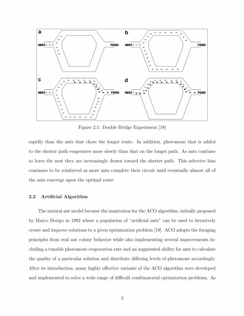
Figure 2.1: Double Bridge Experiment [18]

rapidly than the ants that chose the longer route. In addition, pheromone that is added

to the shorter path evaporates more slowly than that on the longer path. As ants continue

to leave the nest they are increasingly drawn toward the shorter path. This selective bias

continues to be reinforced as more ants complete their circuit until eventually almost all of

the ants converge upon the optimal route

2.2 Artificial Algorithm

The natural ant model became the inspiration for the ACO algorithm, initially proposed

by Marco Dorigo in 1992 where a population of “artificial ants” can be used to iteratively

create and improve solutions to a given optimization problem [19]. ACO adopts the foraging

principles from real ant colony behavior while also implementing several improvements in-

cluding a tunable pheromone evaporation rate and an augmented ability for ants to calculate

the quality of a particular solution and distribute differing levels of pheromone accordingly.

After its introduction, many highly effective variants of the ACO algorithm were developed

and implemented to solve a wide range of difficult combinatorial optimization problems. As

3

the name suggests, combinatorial problems involve finding optimal or near optimal permuta-

tions, links, and combinations of available components. Examples of such problems include

the well known quadratic assignment [20] and traveling salesman problems [21, 22] where

ACO has been proven to be very successful. In addition, ACO has been effectively used to

solve various routing, scheduling, and data mining optimization problems [23].

Despite its success in the combinatorial realm, the algorithm was difficult to apply to

problems of a continuous nature, as the ant colony paradigm is not intuitively applicable to

problems of this type. The components of continuous problems are not partitioned into finite

sets, which the original ant system requires. Several early attempts were made, however to

remedy this shortcoming [24, 25]. The algorithms developed from many of these attempts

borrowed several features of the original ACO model, but they did not follow it closely. In

order to address this issue, Socha and Dorigo developed an algorithm in 2005 they named

ACO-R that more closely adopted the spirit of the original method and could operate in

continuous space natively [26]. The fundamental concept of ACO-R is that the discrete,

probability distributions used in ACO are replaced by probability density functions or PDFs

(see Figure 2.2) in the solution construction phase, and the pheromone distribution is ac-

complished by a large solution archive of weighted PDFs that combine to form a Gaussian

kernel as shown in Figure 2.3.

ACO-R Algorithm Methodology

First, the solution archive is filled with randomly generated solutions. These solutions

are then ranked and given weights based on their quality.

wj =1

qk√

2πexp−(rank(j)− 1)2

k − 1(2.1)

where j is a solutions index in the archive, k is the total number of solutions, and q is a

parameter of the algorithm that determines how the weights are distributed. Lower values

4

Some Variable

Pro

bab

ility

-4 -2 0 2 4

mu = 0, sigma = 0.1mu = 2, sigma = 0.5mu = 0, sigma = 1.0mu = 0, sigma = 3.0

1

0

Figure 2.2: Probability Density Function

Figure 2.3: Gaussian Kernel Construction

5

result in more elitist weight distributions, whereas higher values create more uniform distri-

butions. These weight assignments are analogous to differing pheromone amounts and bias

the selection of higher quality solutions within the search space. Each time a new “ant”

constructs a solution, a new PDF is selected for each dimension from among the solution

archive with a probability proportional to its weight. In this way, all of the solutions are

given a chance to contribute, producing a diverse and robust exploration strategy.

After a specific PDF has been chosen for each component, a new solution is taken from

a normal distribution oriented around its center. The standard deviation of this distribution

is calculated using Equation 2.2.

σij = ζ

k∑r=1

abs(sri − sji )

k − 1(2.2)

This equation sets the standard deviation of each variable i as dependent on the average

distance between the corresponding variable components of all the other k solutions in the

archive. In this way, the characteristics of each Gaussian PDF selected by the ants are

affected by the positions of all the other ants in the archive. Pheromone evaporation rate is

governed by the parameter ζ where a smaller value encourages fast convergence and a larger

value encourages a more thorough exploration of the search domain.

Once m new solutions have been generated, they replace the m worst solutions in the

current archive which is then resorted. This process functions in the same way as pheromone

update by removing the impact of the worst solutions in the current pheromone model. It also

ensures that new solutions will have at least some chance of being selected in the following

iteration, regardless of their fitness, thus encouraging new exploration.

An optional final step of the ACO-R algorithm is to correlate variables using an orthog-

onal gram-schmidt process. For problems involving many variables, however, the computa-

tional effort required to implement this step has been found to be high, significantly reducing

the algorithm’s efficiency. [27,28].

6

Some Design Variable

Fitn

ess

Val

ue

0 2 4 6 8 100

0.5

1

1.5

2

2

4

3

1

(a) Initial Solution Archive

Some Design Variable0 2 4 6 8 10

0

0.5

1

1.5

2

2

4

3

1

(b) PDF Generation

Some Design Variable0 2 4 6 8 10

0

0.5

1

1.5

2

2

4

3

1

new solution

(c) New Solution Creation

Some Design Variable

Fitn

ess

Val

ue

0 2 4 6 8 100

0.5

1

1.5

2

23

1

X

4

(d) New Solution Archive

Figure 2.4: Simple 1-D Illustration of Single Ant Cycle

7

The ordered methodology for the ACO-R algorithm is listed below and a flow chart is

shown in Figure 2.5.

1) Generate an initial solution archive of feasible solutions randomly.

2) Evaluate the quality of each solution in the archive.

3) Rank solutions and create pheromone model by giving each solution a weight.

4) New ants are generated, choosing a solution with a probability proportional to its assigned

weight.

5) Ants sample a PDF formed around each optimization variable of their chosen solution;

combining sampled variables yields a new solution.

6) The solution archive is updated by replacing the m worst solutions in the archive with m

new ant solutions.

7) Return to step 4 until stopping criteria are met.

2.3 Modifications

The basic ACO-R methodology was adopted (sans variable correlation) as the basis

for the algorithm used for this research, while several modifications were made in order to

achieve higher performance:

(A) Elitism

The first modification was that a higher emphasis was placed around searching the

best-so-far solution in the archive in order to achieve quicker convergence. An extra tuning

parameter qmod was created that controlled the probability that a newly generated “ant”

sampled only the area around the best solution. A similar approach was taken by ref [28].

The reason for this modification was that after preliminary testing of the algorithm it was felt

that the original q weighting parameter was not able to give the amount of control wanted

over convergence behavior. When elitism was attempted by setting the weighting parameter

8

Start

Input Initial Parameters

Generate Initial Solution Archive

Evaluate Solution Quality

Rank Solutions and Cre-ate ”Pheromone” Model

Generate New ”Ants” to Fol-low Pheromone Trails andSample Promising Regions

Update Solution Archiveand Pheromone Model

StoppingCriteria

Met?

o

Output Solution

no

yes

Figure 2.5: ACO-R Algorithm Flow

9

Figure 2.6: Effects of parameter “q” on PDF selection

Figure 2.7: Effects of parameter “qmod” on PDF selection

to a very high value, the algorithm tended to converge very quickly, but at the expense

of greatly reduced exploration ability. When the weighting parameter was set low, the

algorithm tended to become unguided and inefficient. By guaranteeing that ants searched a

certain percent of the time around the current best solution, while at the same time allowing

more of the solutions at the bottom end of the archive to contribute, both exploration

and intensification were encouraged. Figures 2.6 and 2.7 illustrate how both the original

q parameter and the added qmod parameter affect the selection probability “P” of a set of

ranked solutions in an archive.

(B) Diversification

A final modification was the addition of a diversification mechanism which was added

in order to combat any potential instances of premature convergence. This was needed to

balance the intensification effect on the algorithm caused by the local search integration.

Each time the local search was called within the algorithm, a subroutine was enacted which

10

generated a temporary, independent ACO routine. An optional feature allowed the tempo-

rary ant colony to avoid searching the area close to where the main colony was converging

by disallowing new solutions containing specified previously used values . A local search was

then performed on the best member found by the rogue colony, and the resulting solution

was then compared to the current best solution for the main ACO program. If the newly

generated solution was found to be better than the current best, it is replaced by the new

solution. Regardless of which solution is chosen as winner, a new solution archive is gener-

ated around the best solution according to a normal distribution with a standard deviation

of 0.5, which was chosen so that the solution archive converges much more aggressively than

the original, yet retains semi-global optimization ability.

(C) Local Search

The second modification was the addition of an integrated local search procedure. Two

local search methods were tested: Hooke and Jeeves pattern search and the Nelder-Mead

simplex method. As will be explained in chapter 3, both methods are derivative-free and are

efficient tools for exploring a small, local region of a design space.

The ordered methodology adopted for the final modified algorithm is as follows:

1) Generate an initial solution archive of feasible solutions.

2) Run an elitist ACO-R cycle for a set number of iterations.

3) Perform local search around best member in the archive.

4) Generate an alternate solution and perform a local search on best member.

5) Compare solutions and re-initialize solution archive around winning member.

6) Repeat steps two through five until stopping criteria are satisfied.

11

Chapter 3

Overview of Competing Algorithms and Complimentary Local Search Methods

3.1 Genetic Algorithm and Particle Swarm Methodology

A total of three different competing optimization methods are used at different points

throughout this study to provide comparison and potential validation of the ACO algorithm.

Two of these methods are fundamentally distinct genetic algorithm implementations. The

first is the binary-coded genetic algorithm IMPROVE (Implicit Multi-objective PaRameter

Optimization Via Evolution) developed by Anderson [29]. This algorithm has been used

multiple times in previous optimization studies and has been shown to be an effective and

robust tool for aerospace design optimization [30–32] and the second is a steady-state, real-

coded GA.

Binary GAs function by converting all of the design variables for a given problem into

a single bit string. A “population” of members is then formed and the resulting bit strings

undergo processes similar to DNA strands in evolutionary theory. Desriable traits are kept

alive through population “breeding” where the strongest members survive, and negative

traits are eventually replaced and eliminated from the gene pool. To maintain diversity and

avoid stagnation, new genetic material is introduced through mutations which occur at a

fixed rate through the lifespan of the algorithm.

Real-coded GAs, unlike binary GAs, are able to operate on a continuous design space

directly and enjoy some advantages over the binary GA such as generally quicker convergence.

Another advantage is that bit resolution is not an issue as is often encountered with binary

methods and binary hamming cliffs can be avoided. A disadvantage of the real-coded GA,

however, is that it may converge too quickly and must rely on properly tuned mutation and

crossover routines to perform effectively.

12

The third optimization method also used for optimizer comparison is a modifed Repul-

sive Particle Swarm Optimization (RPSO) method developed by Mishra [33]. PSO methods,

first introduced by Kennedy and Eberhart [34], mimic the social behavior of a “swarm” of

individuals; each are assigned a position and velocity and they “fly” around the solution

space, working together collectively in a quest to discover quality solutions. PSO methods

are attractive as they are easily implemented and can be directly applied to continuous

design problems. The repulsive variation used for comparison in this work, is designed to

exploit multiple optima in the solution space more thoroughly through the addition of a

trajectory-influencing force which prevents individual swarm members from converging to

the same location.

3.2 Direct Local Search Methods

An often crucial piece of creating a high-performance algorithm, involves the integration

of an effective local search procedure. A class of methods known as direct search methods are

a popular choice for use as a local search. Their attractiveness is based on the fact that they

are often much more numerically efficient than global optimization heuristics in converging

to a solution. Their drawback, however, is that they very easily can become trapped in

local optima. If used as a global optimizer, this behavior is extremely detrimental, but

when used as a local search within an already near-optimal region, rarely has a negative

impact. Two local search methods were considered for integration with the ACO algorithm,

the methodologies of which are explained in the following sections.

3.2.1 Pattern Search

The Pattern Search method was originally developed by Hooke and Jeeves in 1960 [35,36]

as a direct search procedure. The method operates by creating a system of 2N trial points

for an N -dimensional problem by varying each parameter, one at a time, by a specified step

size around the starting base-point. This step size is applied twice; once in a direction larger

13

and once in a direction smaller than value of the original parameter. Once the fitness of each

point is evaluated during this exploratory phase, the point which yields the best solution is

chosen to be the new base point and the process is repeated. If the exploratory moves fail

to yield a new best solution, the step size is reduced by half. Once the radius of the pattern

search has become sufficiently small, the program is terminated.

Figure 3.1: Hooke and Jeeves Pattern Search [37]

3.2.2 Nelder-Mead Simplex

First developed in 1965 [38], the Nelder-Mead Simplex Method is a well-known derivative-

free, nonlinear optimization technique. The simplex algorithm operates by creating a system

of N+1 vertices for an N -dimensional problem which then undergoes a series of reflections

14

and expansions in order to iteratively crawl its way towards a local optimal or near-optimal

solution. For example, in two dimensions, the simplex takes the form of a triangle and in

three dimensions, a tetrahedron. When consecutive iterations of simplex evolution are ani-

mated, it appears as though the simplex structure morphs its way toward a solution, earning

it the common alternative name of the “amoeba method”. Figure 3.2 illustrates the various

ways the simplex structure can evolve within two-dimensional space.

Figure 3.2: 2-D Simplex Morphology

The rules governing simplex behavior can be described as follows:

1) Construct an initial simplex structure around the base point xb.

2) The point with the worst initial fitness xw is reflected through the centroid of the simplex.

3) If the reflected point xr is a new best solution, expand the simplex and reflect further xe.

4) If the new point is not a new best solution, but is still a good solution, start at the top

and reflect again.

5) If the new point is a bad solution, contract the simplex xc and return to step two.

15

6) If successive contractions fail to find an improvement, contract each point x′

within the

simplex structure.

The simplex method is much more aggressive than the pattern search procedure which

allows it to converge much more quickly over a well-behaved solution space. The downside of

this characteristic is that, at times, the simplex may be confused by discontinuous or high-

dimensional problems. In order to combat this, a restart mechanism was encoded within the

simplex subroutine which allowed the algorithm to reset mid-run if needed.

16

Chapter 4

Star-Grain Solid Rocket Motor Design Optimization

4.1 Solid Rocket Motor System Background

A solid rocket motor is composed of a solid propellant, incased in a typically cylindrical

casing. The internal burning surface, known as the grain, is processed into a single basic

geometric form that determines a rockets performance characteristics over time. One of the

more common and versatile grain patterns for tactical missiles is the star grain. This specific

design was chosen as the optimization case for the algorithm. The star grain geometry

definition approach used for this work was described by Barrere [39], and a review of the

analysis method was provided by Hartfield [40]. Star grain patterns can be designed with

as few as three star-points and as many as the upper teens, with an odd number of star

points being more prevalent due to an inherently increased stability. This is because the

star points within an even-numbered motor can sometimes interfere with one another due

to their higher symmetry characteristics. The six design variables used to fully describe star

grain, cross-sectional geometry are shown in Figure 4.1.

4.2 Optimization Procedure

A FORTRAN code developed by Drs. Jenkins, Burkhalter, and Hartfield of the Auburn

University Aerospace Department was available that was capable of determining SRM burn-

back performance. To run the code, a set of design parameters, including the six cross-

sectional parameters shown in Figure 4.1 and the additional three components, grain length,

nozzle expansion ratio, and fuel type bring the total number of optimization variables to

17

Figure 4.1: Star Grain Cross Sectional Geometry [40]

nine. These nine parameters, listed in Table 4.1, determine the performance of an individ-

ual star grain rocket motor and were therefore chosen to be the input parameters for the

optimizer.

Seven of the design variables are inherently continuous, while the number of star points

NSP and the fuel type can only exist as integer values. To avoid an extra complication due to

mixed variable optimization, both the NSP variable and fuel type were encoded as continuous

within the algorithm and then simply converted to the nearest integer value via truncation

whenever the SRM subroutine was called to perform a calculation. This handling of the

integer values creates some reason for concern as it has the potential to create discontinuities

within the solution space. However, the cycling and diversification modifications to the

algorithm proved to be sufficient to handle any such problems in preliminary test runs.

It is often desirable to design a SRM to match a pre-specified flight characteristic as

closely as possible. For this problem, the characteristics to be optimized are the amount

18

Table 4.1: SRM Optimization Design Parameters

Design Variable Description

Rpvar = (Rp + f)/Rbody Propellant outer radius ratioRivar = Ri/Rp Propellant inner radius ratio

Ro Outer grain radiuseps Star widthNsp Number of star pointskfuel Propellant fuel typegl Grain length

fvar = f/Rp Fillet radius ratioDstar Nozzle expansion ratio

of thrust produced by the SRM and its internal chamber pressure. The success of the

optimization is determined by how closely a SRM can be designed to match a specified

chamber pressure or thrust trend with respect to time. The ability to match this curve will

be calculated by taking the average root mean squared error or RMSE over the course of an

alloted burn time, where RMSE is the sum of the variances between the desired curve and

the curve generated by the best solution found by the optimizer. This was accomplished by

breaking the SRM performance-time data into intervals of 0.01 seconds using simple linear

interpolation between output data points generated by the code.

In order to determine the best local search procedure to use with the ACO algorithm

for the SRM burnback cases, it was allowed to run without the local search procedure twenty

different times. The points generated by each run were then operated on by both the pattern

search and simplex methods. Each local search procedure was allowed to run until either

convergence, or after 500 function calls were completed – whichever came first. The simplex

method proved to be the better performer for this problem as can be seen by the results

in Table 4.2, and was adopted as the local search procedure for the SRM curve-matching

problems.

19

Table 4.2: Local Search Performance Comparison

Method Average Solution Improvement (%)

N.M. Simplex 72.8Pattern Search 46.2

4.3 SRM Curve Matching Problems and Results

Three cases were considered in order to test the algorithm:

Random Burn Profile

This problem was chosen to be the first attempted; it was the easiest challenge since

a solution was guaranteed to exist within the solution space. For this reason, the problem

could be used to determine initially if the optimizer was, in fact, working correctly. Also,

it functioned as a baseline for parameter tuning purposes. To set up the objective function,

each design variable was given a single randomly assigned value within its design range and

this set of values was input into the SRM code. The program then output corresponding

data about the thrust and chamber pressure over time which was then used as the objective

function for the optimizer.

The algorithm was able to achieve a very close match for the first problem, obtaining a

best solution of only 0.0077 percent RMSE and never returning a solution worse than 0.0724

percent RMSE, demonstrating a high degree of consistency. The best grain design found by

the optimizer is shown in Figure 4.2 and the resulting burn profile is shown in Figure 4.3.

Neutral Burn Profile

For the second problem, a neutral burn match was attempted where the SRM optimizer

was tasked with the job of maintaining a constant chamber pressure of 500 psia over a

twenty-second burn duration. As illustrated in Figure 4.4, a close match of 0.109 percent

RMSE was found for the problem. The optimized grain cross-section is shown in Figure 4.5.

20

Figure 4.2: Optimized SRM Grain Geometry - Random Burn

Figure 4.3: Chamber Pressure vs Time Curve - Random Burn Profile

21

Time (s)

Ch

ambe

rP

ress

ure

(psi

a)

0 5 10 15 20460

480

500

520

540

Objective CurveOptimized Curve

0.051% RMSE

Figure 4.4: Chamber Pressure vs Time Match - Neutral Burn Profile

Figure 4.5: Optimized SRM Grain Geometry - Neutral Burn

22

Regressive-Progressive Burn Profile

A regressive-progressive motor burns in such a way that it produces a gradually dimin-

ishing thrust up to a certain point along its burn duration, at which point thrust begins to

increase until the motors tail-off point is reached. A problem of this type was created where

thrust begain at 80000 psia, was reduced to 60000 psia at ten seconds, and then increased

back to 80000 psia after twenty seconds. A thrust curve was used in place of a pressure curve

for this optimization attempt. This does not affect the problem significantly as changes in

pressure were directly correlated to changes in thrust for the set of design variables used.

This problem was expected to much more difficult to solve than the first, as the sudden,

linear turning point cannot be exactly produced due to the transient burn characteristics of

an SRM. As expected, this curve profile was very difficult to match, but the optimizer was

able to achieve an RMSE of between 0.610 percent, shown in Figure 4.6, and 0.674 percent.

The optimized grain cross-section is shown in Figure 4.7.

Summary

Overall, the results show that the algorithm is very effective in solving the SRM opti-

mization problems. However there was no way to directly compare the results to previous

work done with other optimizers for this problem due to ambiguity within the published

design variable limits. For this reason, fair validation of the ACO algorithm against other

methods was unattainable and another design problem without this deficiency was sought.

23

Time ( s )

Thr

ust

(lb

f)

0 5 10 15 2055000

60000

65000

70000

75000

80000

85000

Objective CurveOptimized Curve

0.610% RMSE

Figure 4.6: Thrust vs Time Curve - Regressive-Progressive Burn

Figure 4.7: Optimized SRM Grain Geometry - Regressive Progressive

24

Table 4.3: Summary of Results and Optimized SRM Geometries

Design Parameter Random Burn Neutral Burn Regressive-Progressive

Rpvar 0.583262 0.679595 0.450154Rivar 0.190164 0.199874 0.143454Nsp 7 5 5fvar 0.063335 0.0799974 0.0200000eps 0.811286 0.6952298 0.5463125rbod 15.9544625 34.9967667 24.1715989gl 9.9964089 3.2935126 6.0560694

diath 0.24703012 0.2195772 0.200886139ftype 4 3 1

Best Solution (%RMSE) 0.0077 0.610 0.051Worst Solution (%RMSE) 0.0724 0.674 0.169

Average Solution (%RMSE) 0.0265 0.629 0.109

25

Chapter 5

Solid Motor Sounding Rocket Optimization

5.1 Sounding Rocket System Description

After the SRM curve matching problems, the next step in testing the algorithm was to

attempt a sounding rocket design optimization. This problem presented an opportunity to

try the ACO algorithm on a slightly more complicated problem as well as to attempt vali-

dation of the ACO algorithm by comparing its performance with other known optimization

methods. In a previous study conducted by Badyrka [49], three algorithms were tested on

their ability to design a sounding rocket to meet a set of three specific performance goals.

These goals were specified for the sounding rocket to carry a payload of 70lb to a burnout

altitude of 50,000ft and burnout velocity of 1,000ft/sec with an additional emphasis on min-

imizing takeoff weight. The “fitness” of each missile design found is calculated according to

equation 5.1.

Fitness = abs(AltitudeError) + abs(V elocityError) +Weight

1000(5.1)

The code used for the optimizer study by ref [49] was availabe through the Auburn Uni-

versity Dept. of Aerospace Engineering. It works by processing the input design parameters

to determine geometry and burn characteristics for solid rocket motors using subroutines

similar to those used in the curve-matching problem. In addition, the code calculates the

total weight of the sounding rocket system, first by determining the weight of the structures

outside of the motor, including the case, joints, end cap and nozzle, and then adding them

to the combined weight of the payload, propellant, and ignition system. A total of eleven

design parameters, listed in Table 5.1 are required for a complete sounding rocket model.

26

Table 5.1: Sounding Rocket Design Parameters

Design Variable Description

Rpvar = (Rp + f)/Rbody Propellant outer radius ratioRivar = Ri/Rp Propellant inner radius ratio

Ro Outer grain radiuseps Star widthNsp Number of star pointsptang Star point anglekfuel Propellant fuel typegl Grain length

fvar = f/Rp Fillet radius ratioDiath Nozzle throat diameterRatio Nozzle expansion ratio

The three optimization methods described previously were tested and the results were

availabe from the work of ref [49]. Using identical design constraints and an equivalent

number of 250,000 allowable function calls, the ACO algorithm was applied to the same

problem.

It should be noted that the local search option of the modified ACO algorithm was

turned off for this and the remaining problems attempted in this study involving comparisons

to other optimization schemes. This was done in order to avoid an unfair comparison, as the

competing algorithms did not possess a local search ability.

5.2 Sounding Rocket Results

As seen in Table 5.2 and Figure 5.1, the ACO algorithm was able to find a significantly

better solution than RPSO, and was also able to outperform both of the GAs. As seen

in the solution convergence history (Figure 5.2), ACO was able to accomplish this using

significantly fewer function calls than any of the competing methods. The algorithm was

also able to avoid stagnation, and continued to find improving solutions very deep into its

run.

27

Grain Radius ( in )-30 -20 -10 0 10 20 30

Fitness = 2300.14

(a) RPSO Best

Grain Radius ( in )-30 -20 -10 0 10 20 30

Fitness = 33.34

(b) Binary GA Best

Grain Radius ( in )-30 -20 -10 0 10 20 30

Fitness = 42.14

(c) Real GA Best

Grain Radius ( in )-30 -20 -10 0 10 20 30

Fitness = 18.59

(d) ACO Best

Figure 5.1: Best Sounding Rocket Solutions Found by Optimizers

28

Number of Function Calls

Sou

ndin

gR

ocke

tFitn

ess

0 50000 100000 150000 200000 250000101

102

103

104

Mod-ACOBinary GAReal GA

Convergence History

Figure 5.2: Optimizer Convergence History

29

Table 5.2: Sounding Rocket Optimization Results

Design Parameter RPSO Binary GA Real GA ACO

Propellant type 7 8 8 8Rpvar 0.522325 0.535039 0.754812 0.513013Rivar 0.010100 0.221373 0.010000 0.364549Nsp 8 11 17 12Fvar 0.063567 0.040045 0.014708 0.010000epsilon 0.472595 0.686667 0.341543 0.839910

Star point angle 1.275354 5.677166 8.909556 7.241508Grain length 239.7870 301.3699 241.5387 243.2500

Outer grain radius 23.76000 22.95238 19.06190 18.89172Throat Diameter 19.80000 12.86399 19.49395 12.34742Expansion Ratio 1.915620 3.842520 3.246192 6.000074

Altitude at BO 47760.86 50004.55 49999.98 49996.90Velocity at BO 960.67 997.71 968.22 999.63Initial weight 21672.41 26505.14 10339.07 15119.78

Total Fitness 2300.14 33.34 42.14 18.59

In addition, by the end of the alotted run time, nine distinct solutions excluding the

best solution were found with a total fitness of less than 30.0 which, remarkably, is better

than any solution found by the GAs or RPSO. The degree of diversity found within the

solutions is demonstrated by four example SRM grain designs in Figure 5.3. Table 5.3

further demonstrates solution diversity by showing that of the multiple SRM grain designs

discovered by ACO, eight had a unique number of star points.

Table 5.3: Sounding Rocket Multiple Solutions

No. Star Points Best Solution Fitness No. Star Points Best Solution Fitness

6 29.86 12 18.598 23.16 13 28.279 24.86 14 28.4311 29.20 15 22.88

30

Grain Radius ( in )-30 -20 -10 0 10 20 30

Fitness = 24.86

(a) Alternate Solution 1

Grain Radius ( in )-30 -20 -10 0 10 20 30

Fitness = 21.46

(b) Alternate Solution 2

Grain Radius ( in )-30 -20 -10 0 10 20 30

Fitness = 23.16

(c) Alternate Solution 3

Grain Radius ( in )-30 -20 -10 0 10 20 30

Fitness = 29.86

(d) Alternate Solution 4

Figure 5.3: Example Alternate Sounding Rocket Solutions

31

Chapter 6

Description of 6DOF Missile System

The primary tool used for this study was a missile design program developed by Burkhal-

ter, Jenkins, Hartfield, Anderson, and Sanders, described in their paper “Missile Systems

Design Optimization Using Genetic Algorithms” [47]. The missile design codes developed

are capable of creating and flying preliminary level engineering models of missiles powered by

a single-stage solid propellant motor. The codes have been validated as an effective prelimi-

nary design tool and have been proven to be a reliable tool for aerospace design applications,

having been successfully utilized in many previous optimization studies [8, 9, 43].

Before a viable 6-DOF trajectory can be simulated by the missile program for a given

design, several processes must first occur.

1) The main program receives input from files which contain values for constants that are

necessary for proper code operation. A break-down of these constants is shown in table 6.2.

2) The propulsion system is modeled using grain geometries specified by the input to develop

the thrust profile for the motor.

3) Mass properties are calculated and used to determine the center of gravity and moments

of inertia for all components included in the system.

4) Aerodynamic properties for the missile are calculated using the non-linear, fast predictive

code AERODSN [48].

5) The resulting propulsion, mass, and aerodynamic characteristics are then integrated with

the equations of motion to determine the complete 6DOF flight profile for the missile.

32

Begin program

Input initial constants

Input optimizer settings

Create initial population

Run optimizer (ACO or GA)

Determine flight characteristicso

MassAerodynamics

Propulsion

Simulate 6-DOF missile trajectory

StoppingCriteria

Met?

o

Terminate program

no

yes

Figure 6.1: Single Stage Solid Missile System

More complicated than the SRM curve matching and sounding rocket systems, the

6DOF missile system presents opportunities for more difficult optimization problems that

are important in testing the abilities of the ACO algorithm. The complete set of design

parameters that can be varied by an optimizer is shown in Figure 6.1. The entire set creates

opportunities for 35-variable optimization problems. Three such problems, each of increasing

difficulty, were attempted and are described in the following sections.

33

Table 6.1: List of Single Stage Solid Missile Design Variables

Missile Geometry Propellant Properties Autopilot Controls

Nose radius ratio = rnose/rbody Fuel type Autopilot On Delay TimeNose length ratio = lnose/dbody Propellant outer radius ratio Initial launch angle (deg)

Fractional nozzle length ratio = f/ro Propellant inner radius ratio Pitch multiplier gainNozzle throat diameter/dbody Number of star points Yaw Multiplier gainTotal length of stage1/dbody Fillet radius ratio - f/rp Initial elevator angle (deg)Diameter of stage 1 (dbody) Epsilon - star width Gainp2 - gain in pitch angle def

Wing exposed semi-span = b2w/dbody Star point angle B2var = b2vane/rexitWing root chord crw/dbody Time step to actuate controlsWing taper ratio = ctw/crw Gainy2 - gain in yaw angle dif

Leading edge sweep angle wing (deg) Deltx for Z correctionsxLEw/lbody Deltx for Y corrections

Tail exposed semi-span = b2t/dbodyTail root chorse = Crt/dbody

Tail taper ratio = ctt/crwLeading edge sweep angle tail ( deg)

xTEt/LbodyNozzle Exit Dia/dbody

34

Table 6.2: Classification of Initial Missile Design Code Constants

Component Section No. of Design Variables

Constants 22Material Densities 6

Program Lengths, Limits, and Constants 31Constants and Set Numbers 25

Launch Data Initiation 16Target Data 6

Optimizer Goals (outdata variables) 20Auxiliary Variables 21

List of Optimizer Variables Passed to Objective Function 35Total Set of Missile Variables 40

Guidance and Plotting Variables 29Component Densities 30

Masses 30Center of Gravity 30Moments of Inertia 60Component Lengths 30

Components’ Axial Starting Point 30Required and computed data for Aero 30

Other Dimensions 16Internal Solid Rocket Grain Variables 14

Nozzle and Throat Variables 23Additional Computed Stage Variables 8

35

Chapter 7

Single Stage Solid Missile System Optimizer Comparisons

In addition to the sounding rocket problem, the study by Badyrka also compared the

same three algorithms in their ability to design a single-stage solid rocket system to hit a

target located at a specified range. The fitness for each design was defined according to

equation 7.1.

Fitness =abs(Range−DesiredRange)

10(7.1)

As these tests have only a simple singular objective, it should be expected that the design

solution space contains an extremely wide variety of missile designs capable of meeting this

objective. Although simple, this set of testing was an important stepping stone for more

complicated probems involving the 35-variable, single stage solid missile system.

7.1 Match Range - 250,000 ft

The goal of the first test was to design a missile capable of hitting a position located

a distance of 250,000 ft from the launch point. It should be noted that a miss distance of

roughly one foot is practically considered a hit; therefore the significantly greater precision

is for academic purposes only. For this problem, each optimizer was allowed 100,000 calls to

the objective function.

Again, ACO was able to outperform both RPSO and the GAs, achieving a fitness of at

least 2.21E-12 before being rounded to zero due to the precision tolerance of the FORTRAN

program. The best results obtained by each algorithm are listed in Table 7.1.

36


Mis

sile

Fitn

ess

101 102 103 104 10510-12

10-10

10-8

10-6

10-4

10-2

100

102

104

Binary GAReal GAACO-Mod

Figure 7.1: Convergence History - Match 250,000 ft

Table 7.1: Results for Range Matching Problem - 250,000 ft

Optimizer Best Missile Fitness

RPSO 0.142455Binary GA 7.41949E-05Real GA 2.24332E-08

ACO 2.21E-12

37

As with the sounding rocket problem, the algorithm was also able to find multiple near-

optimal solutions. Three of these solutions are shown in Figure 7.2. Each missile design

shown has a fitness of less than 2.21E-12 and was obtained during the course of the main

run.

7.2 Match Range - 750,000 ft

The second optimization design test was identical to the first, only this time the target

range was set as 750,000 ft from the launch point. This test was important as matching this

extended range involves searching a different region of the solution space and served to add

validation to the results obtained from the shorter-ranged test.

Similar results were found for the best 750,000 ft missile solution as recorded in Table

7.2. Solution diversity is again illustrated with depictions of three unique missile designs in

Figure 7.4.

38

(a) Missile Design 1

(b) Missile Design 2

(c) Missile Design 3

Figure 7.2: Example Alternate Sounding Rocket Solutions - 250,000 ft

39


Mis

sile

Fitn

ess

102 103 104 10510-12

10-10

10-8

10-6

10-4

10-2

100

102

104

Binary GAReal GAACO-Mod

Figure 7.3: Convergence History - Match 750,000 ft

Table 7.2: Results for Range Matching Problem - 750,000 ft

Optimizer Best Missile Fitness

RPSO 0.43482Binary GA 5.76720E-05Real GA 2.48252E-06

ACO 2.21E-12

40

(a) Missile Design 1

(b) Missile Design 2

(c) Missile Design 3

Figure 7.4: Example Alternate Sounding Rocket Solutions - 750,000 ft

41

7.3 Match a Single Trajectory

The second part of the single-stage testing significantly increases the difficulty of the

optimization by increasing the number of performance objectives from one to four. The first

problem attempted was to design a missile to match a single trajectory. The fitness of a

given missile design is calculated based on how well it matches four different flight objectives:

(1) Time of flight (2) Time until burnout (3) Apogee match and (4) Range of flight. Each

objective is weighted and the final fitness is given by equation 7.2.

Fitness =RangeError

10+ApogeeError

10+TOFError

1+TBOError

1(7.2)

With the exception of some tampering with the population size and restart cycles, the

tuning parameters for the GA were not varied for the trajectory matching problems, as the

default settings have been shown to be successful with approximately identical settings in

the past for similar problems.

It should be noted, that since the modified ACO algorithm was designed to work in rapid,

fast-converging cycles, an extra effort was made in an attempt to avoid an unfair comparison

with the binary GA. In addition to the default setting of 200 population members, an extra

GA program was coded whereby the population size was reduced so that the GA also worked

in a series of fast converging cycles. Both methods were run for each trajectory case, and

the results from the best of the two methods were then chosen to be used for all trajectory-

matching comparisons with ACO in this study.

Again, the modified ACO algorithm was able to find a better solution than the binary

GA, reaching a better solution than was found for the entire GA run within 4,000 function

calls as can be seen in Figure 7.5. The difference in the final fitness values, however, was not

as large as was found in the previous problems. It is difficult to tell whether this could be

because the missile fitness has neared a lower limit or because the advantage of ACO over

the GA is not as significant for this problem.

42


Mis

sile

Fitn

ess

0 10000 20000 30000 40000100

101

102

103

104

Binary GAACO

Figure 7.5: Single Trajectory Convergence History

The trend for ACO to find multiple, high-quality solutions for a problem continued as

a total of nine different solutions were found with fitness values below 10.00 during a single

run of the ACO algorithm as shown in Table 7.4.

7.4 Match Three Trajectories

The most difficult optimization problem attempted involved designing a single missile

to match three separate trajectories. This creates a much more complex solution space with

an increased ability to confuse an optimizer. The trajectories used had differing flight ranges

43

Table 7.3: Single Trajectory Results

Design Parameter Best Solution - Binary GA Best Solution - ACO

rnose/rbody 0.380379974842E+00 0.398375660181E+00lnose/dbody 0.158920001984E+01 0.170792245865E+01

fuel type 0.433333349228E+01 0.452283191681E+01rpvar 0.564000010490E+00 0.536266922951E+00rivar 0.838933363557E-01 0.889812931418E-01

number of star points 0.733333349228E+01 0.732177782059E+01fvar 0.626666620374E-01 0.684898123145E-01

epsilon 0.899996697903E+00 0.904991567135E+00star point angle 0.100000000000E+02 0.100751829147E+02

fractional nozzle length 0.620000004768E+00 0.722629070282E+00dia throat/ dia body 0.292666673660E+00 0.272233247757E+00

fineness ratio 0.565681743622E+01 0.584986734390E+01diameter of stage 1 0.114043736458E+01 0.105696105957E+01

wing semispan/dbody 0.500000023749E-03 0.550335331354E-03wing root chord/dbody 0.600000028498E-03 0.560724933166E-03

taper ratio 0.850000023842E+00 0.868137657642E+00wing LE sweep angle 0.400999984741E+02 0.400922050476E+02

xLEw/lbody 0.500000000000E+00 0.443633228540E+00tail semispan/dbody 0.117277395725E+01 0.109947204590E+01

tail root chord/dbody 0.112769865990E+01 0.113723444939E+01tail taper ratio 0.634329974651E+00 0.556621313095E+00LE sweep angle 0.185806465149E+02 0.110512800217E+02

xTEt/lbody 0.990000009537E+00 0.990520238876E+00auto pilot delay time 0.139583384991E+01 0.131948125362E+01initial launch angle 0.100000001490E+00 0.744342575073E+02

pitch multiplier gain 0.600000000000E+01 0.459953069687E+01yaw multiplier gain 0.440000009537E+01 0.394029784203E+01

nozzle exit dia/dbody 0.734000027180E+00 0.721238851547E+00initial pitch cmd angle -0.800000011921E+00 -0.118590712547E+01angle dif gain in pitch 0.466666650772E+01 0.467941570282E+01

warhead mass 0.228666674805E+04 0.229966894531E+04time step to actuate nozzle 0.100000000000E+01 0.971418082714E+00

angle dif gain in yaw 0.442857116461E+00 0.488472193480E+00initial launch direction -0.100000001490E+00 0.895773162842E+02initial pitch cmd angle 0.100000004750E-02 0.129012929392E-03

missile fitness 10.74 8.20

44

X

Y

Z

Final Fitness = 8.20

Figure 7.6: 3-D Optimized Missile Design - 164 km trajectory

45

(a) GA Best Solution

(b) ACO Best Solution

Figure 7.7: Optimized Missiles - 164km Trajectory

46

Missile Range (km)

Mis

sile

Alti

tud

e(k

m)

0 20 40 60 80 100 120 140 160 1800

20

40

60

80

100

120

140

160

Target TrajectoryOptimized Trajectory

Figure 7.8: Optimized Trajectory Match - 164 km

47

Table 7.4: Multiple Alternate Solutions - 164 km Trajectory

Solution No. Missile Fitness Solution No. Missile Fitness

1 9.32 6 8.552 9.49 7 9.453 9.73 8 8.954 9.83 9 9.915 9.95 10 9.27

of 117 km, 164 km, and 221 km, respectively. Final missile fitness is calculated by simply

calculating the fitness with respect to each trajectory using equation 7.2 as for the single

trajectory problem and then adding them together.

TotalF itness = fitness117 + fitness164 + fitness221 (7.3)

The ACO algorithm performed extremely well compared to the Binary GA for the three-

trajectory problem. Not only was the best ACO solution significantly better than the best

GA solution, but five different solutions were found with a fitness of less than 100.00, less

than half of what the binary GA was able to achieve using the same number of function

calls.

48

Table 7.5: Three Trajectory Results

Design Parameter Best Solution - Binary GA Best Solution - ACO

rnose/rbody 0.400400012732E+00 0.404787927866E+00lnose/dbody 0.182120001316E+01 0.187957513332E+01

fuel type 0.433333349228E+01 0.427150249481E+01rpvar 0.527333319187E+00 0.552933871746E+00rivar 0.862400010228E-01 0.842992588878E-01

number of star points 0.600000000000E+01 0.729311084747E+01fvar 0.706666633487E-01 0.634117126465E-01

epsilon 0.879998028278E+00 0.967089176178E+00star point angle 0.101000003815E+02 0.100787239075E+02

fractional nozzle length 0.759999990463E+00 0.753344714642E+00dia throat/ dia body 0.285333335400E+00 0.280373215675E+00

fineness ratio 0.603144073486E+01 0.596240997314E+01diameter of stage 1 0.112533271313E+01 0.120006358624E+01

wing semispan/dbody 0.600000028498E-03 0.508977915160E-03wing root chord/dbody 0.600000028498E-03 0.551881676074E-03

taper ratio 0.949999988079E+00 0.912369012833E+00wing LE sweep angle 0.400000000000E+02 0.400045547485E+02

xLEw/lbody 0.400000005960E+00 0.463914483786E+00tail semispan/dbody 0.112554800510E+01 0.111973583698E+01

tail root chord/dbody 0.111333334446E+01 0.114281380177E+01tail taper ratio 0.603575289249E+00 0.529041469097E+00LE sweep angle 0.139354839325E+02 0.345442543030E+02

xTEt/lbody 0.990999996662E+00 0.990521907806E+00auto pilot delay time 0.139583384991E+01 0.140671408176E+01initial launch angle 0.333333313465E-01 0.751682662964E+02

pitch multiplier gain 0.493333339691E+01 0.514768838882E+01yaw multiplier gain 0.253333330154E+01 0.324552249908E+01

nozzle exit dia/dbody 0.840666711330E+00 0.973625361919E+00initial pitch cmd angle -0.173333334923E+01 -0.768583893776E+00angle dif gain in pitch 0.359999990463E+01 0.349795055389E+01

warhead mass 0.214000000000E+00 0.212670410156E+04time step to actuate nozzle 0.100000000000E+01 0.953021109104E+00

angle dif gain in yaw 0.442857116461E+00 0.706241011620E+00initial launch direction 0.100000001490E+00 0.897416076660E+02initial pitch cmd angle 0.000000000000E+00 0.492134888191E-03

missile fitness 229.84 46.31

49

Table 7.6: Multiple Alternate Solutions - Three Trajectory Problem

Solution No. Missile Fitness Solution No. Missile Fitness

1 61.35 3 83.042 65.37 4 93.22


Mis

sile

Fitn

ess

10000 20000 30000 40000101

102

103

104

Binary GAACO

Figure 7.9: Three-Trajectory Convergence History

50

(a) GA Best Solution

(b) ACO Best Solution

Figure 7.10: Optimized Missiles - Three Trajectories

51

X

Y

Z

Final Fitness = 46.31

Figure 7.11: 3-D Optimized Missile Design - Three Trajectories

52

Missile Range (km)

Mis

sile

Alti

tude

(km

)

0 50 100 150 200 2500

20

40

60

80

100

120

140

160Target Trajectory - 117kmOptimized Trajectory - 117kmTarget Trajectory - 164kmOptimized Trajectory - 164kmTarget Trajectory - 221kmOptimized Trajectory - 221km

Figure 7.12: Optimized Three-Trajectory Matches

53

Chapter 8

Local Search Testing

The trajectory matching optimization routine was run once again, but this time the

local search capability was activated for the ACO algorithm. In addition to the 164 km

trajectory, matching of the individual 117km and 221km trajectories was also attempted.

Each time the algorithm would reach a local convergence point before re-cycling, both

the pattern search method and the simplex method were called to search around the best

solution found in the area of convergence. Each local search procedure was allowed 310

function calls, chosen to be approximately one-third of the average number of calls needed

by each ACO mini-cycle to reach near-convergence. To more thoroughly test each method,

three different initial step sizes were used, corresponding to 0.5, 1.0, and 2.0 percent of the

range of each design variable. A total of 32 separate local search runs were performed around

a variety of solutions, the results of which are shown in Table 8.1.

Both local search methods were nearly always able to improve on a given solution.

For the individual trajectories, the Simplex Method was consistently able to obtain slightly

better solutions than the pattern search. For the three-trajectory case, however, the pattern

Table 8.1: Local Search Improvements - 164km Trajectory

Local Search Method Initial Step Size (% range) Average Improvement (%)

Pattern Search 0.5 8.45411.0 7.10932.0 9.7011

Simplex Method 0.5 12.33161.0 11.16572.0 11.5382

54



Pattern Search 0.5 9.72671.0 6.43172.0 7.3947

Simplex Method 0.5 12.11681.0 13.03202.0 11.0361



Pattern Search 0.5 17.61231.0 16.55212.0 15.3737

Simplex Method 0.5 19.49251.0 19.91862.0 20.8828

Table 8.4: Local Search Improvements - Three Trajectories


Pattern Search 0.5 4.28241.0 5.51682.0 6.9079

Simplex Method 0.5 4.68371.0 4.88812.0 4.6092

55

search seemed to work more effectively. This might be because the three-trajectory problem

is more complex and was able to confuse the simplex.

The single trajectory results were very interesting as a previous study had concluded

that the pattern search was the significantly better optimization method when integrated

within a hybrid, GA/PSO optimizer. The local search application in the two instances was

very different, however, as it was used as the main driver of the optimization within the

hybrid scheme whereas in this study, its application was strictly focused on a small region

of space to improve upon already near-optimal solutions.

For this particular trajectory match, the Simplex Method was able to obtain slightly

better solutions than the pattern search for every step size used. This result was very inter-

esting as a previous study had concluded that the pattern search was the better optimization

method when integrated within a hybrid, GA/PSO optimizer. The local search application

in the two instances was very different, however, as it was used as the main driver of the

optimization within the hybrid scheme whereas in this study, its application was strictly

focused on a small region of space to improve upon already near-optimal solutions.

56

Chapter 9

Summary and Recommendations

The design optimization results generated by the modifed ACO algorithm demonstrate

its ability to be competitive, if not more effective, than many established methods. For each

problem where a comparison was attempted, the ACO algorithm converged more quickly

and found a better solution than competing optimization algorithms. Additionally, it was

found to be capable of locating muliple optimal solutions within the design space for the

sounding rocket and missile trajectory problems. However, more extensive testing of the

algorithm needs to be performed and the results compared to those obtained from a more

complete set of modern, high-performance optimization schemes.

There could be many reasons as to why the ACO algorithm performed better than

RPSO and the GAs for this particular set of problems. First, the algorithm was developed

and tuned in order to achieve high performance on the SRM curve-matching problems,

and although problems attempted later (e.g. 6DOF trajectory) were vastly more complex

than the original problem, there may have been some advantages gained by designing the

algorithm to perform well on problems involving the SRM code. Additionally, it is the

author’s opinion that GAs (in particular binary coded GAs) do not compare well with more

modern optimization methods when used as the sole optimizer for a problem. They seem to

be very good at avoiding stagnation, but are simply not aggressive enough to locate quality

optima in a reasonable number of function calls. However, they do seem to work well as a

component of hybrid optimization algorithms that integrate the stability of GAs with the

increased aggressiveness of other optimization routines.

Preliminary results involving local search integration within the ACO algorithm show

a strong indication that they are effective in improving solutions found by the main ACO

57

driver. Results indicate that the Nelder-Mead Simplex Method and the Pattern Search pro-

cedure each have advantages over the other depending on how they are used and on what

type of problem is being attempted. For the majority of problems attempted in this study

it seems that the simplex method is more efficient when used as a purely local procedure.

Additional future work that could be performed includes :

A) Fine-tuning of the ACO algorithm parameters for each of the problems attempted in this

study to determine how solutions could be improved.

B) Application of the algorithm to even more complex design problems such as liquid pro-

pellant and multiple stage missile system optimization.

C) Expansion of the missile design limits for the trajectory matching problems as the limits

used for this study are quite narrow. This would further increase the optimization difficulty

while allowing a greater variety of missile designs to be found to match a particular trajec-

tory.

D) Further testing of the local search methods. Additional work on improving the local ser-

ach performance remains to be attempted. It would be interesting to perform more extensive

testing of Simplex, Pattern Search, and other methods in order to have a better idea of their

comparative capabilities.

58

Bibliography

[1] Karr, C.L., Freeman, L.M., and Merideth, D.L. ”Genetic algorithm based fuzzy con-trol of spacecraft autonomous rendezvous,” NASA Marshall Space Flight Center, FifthConference on Artificial Intelligence for Space Applications, 1990.

[2] Krishnakumar, K, Goldberg, D.E., ”Control system optimization using genetic algo-rithms”, Journal of Guidance, Control, and Dynamics, vol. 15, no. 3, May-June 1992.

[3] Krishnakumar, K., Goldberg, D.E., ”Control system optimization using genetic algo-rithms”, Journal of Guidance, Control, and Dynamics, vol. 15, no. 3, May-June 1992.

[4] Perhinschi, M.,G., ”A modified genetic algorithm for design of autonomous helicoptercontrol system,” AIAA-97-3630, presented at the AIAA Guidance, Navigation, andControl Conference, New Orleans, LA, August 1997.

[5] Mondoloni, S., A Genetic Algorithm for Determining Optimal Flight Trajectories, AIAAPaper 98-4476, AIAA Guidance, Navigation, and Control Conference and Exhibit, Au-gust 1998.

[6] Anderson, M.B., Using Pareto Genetic Algorithms for Preliminary Subsonic Wing De-sign, AIAA Paper 96-4023, presented at the 6th AIAA/NASA/USAF MultidisciplinaryAnalysis and Optimization Symposium, Bellevue, WA, September 1996.

[7] Perez, R.E., Chung, J., Behdinan, K., Aircraft Conceptual Design Using Genetic Al-gorithms, AIAA Paper 2000-4938, Presented at the 8th AIAA/USAF/NASA/ISSMOSymposium on Multidisciplinary Analysis and Optimization, September 2000.

[8] Hartfield, Roy J., Jenkins, Rhonald M., Burkhalter, John E., Ramjet Powered MissileDesign Using a Genetic Algorithm, AIAA 2004-0451, presented at the forty-secondAIAA Aerospace Sciences Meeting, Reno NV, January 5-8, 2004.

[9] Jenkins, Rhonald M., Hartfield, Roy J., and Burkhalter, John E., Optimizing a SolidRocket Motor Boosted Ramjet Powered Missile Using a Genetic Algorithm, AIAA 2005-3507 presented at the Forty First AIAA/ASME/SAE/ASEE Joint Propulsion Confer-ence, Tucson, AZ, July 10-13, 2005.

[10] Burger, Christoph and Hartfield, Roy J., Propeller Performance Optimization usingVortex Lattice Theory and a Genetic Algorithm, AIAA-2006-1067, presented at theForty-Fourth Aerospace Sciences Meeting and Exhibit, Reno, NV, Jan 9-12, 2006.

59

[11] Chernyavsky, B., Stepanov, V., Rahseed, K., Blaize, M., and Knight, D., ”3-D hy-personic inlet optimization using a genetic algorithm”, 34th AIAA/ASME/SAE/ASEEJoint Propulsion Conference and Exhibit, July 1998.

[12] Wang, G. ”Multiple UAVs Routes Planning Based on Particle Swarm OptimizationAlgorithm”, 2nd International Symposium on Information Engineering and ElectronicCommerce, July 23-35, 2010.

[13] Wall, D.L., ”Optimum Propeller Design for Electric UAVs”, Master’s Thesis, AuburnUniversity, August 2012.

[14] Wickramasinghe, U.K., Carrese, R., and Li, X., ”Designing airfoils using a referencepoint based evolutionary many-objective particle swarm optimization algorithm”, IEEECongress on Evolutionary Computation, pp. 1-8, 2010.

[15] Nejat, A., Mirzabeygi, P., and Panah, M.S., ”Aerodynamic shape optimization usingimproved territorial particle swarm algorithm”. ASME 2012 International MechanicalEngineering Congress and Exposition, Houston, TX, Nov 2012.

[16] Goss, S., Aron, S., Deneubourg, J.L., and Pasteels, J.M., Self-organized Shortcuts inthe Argentine Ant, Naturwissenschaften, Vol. 76, pp. 579-581, 1989.

[17] Hoelldobler, B., and Wilson, E. The Ants, Belknap Press, 1990.

[18] Cordon, O., Herrera, F., and Stutzle, T., A review on the ant colony optimizationmetaheuristic: Basis, models and new trends., Mathware and Soft Computing, Vol. 9,pp. 141-175, 2002.

[19] Dorigo, M., Optimization, Learning, and Natural Algorithms, PhD thesis, Politecnicodi Milano, Italie, 1992.

[20] Sttzle,T., ”MAX-MIN Ant System for the quadratic assignment problem,” TechnicalReport AIDA-97-4, FB Informatik, TU Darmstadt, Germany, 1997.

[21] Bianchi, L, Gambardella, L.M., and Dorigo, M., An ant colony optimization approachto the probabilistic traveling salesman problem, PPSN-VII, Seventh International Con-ference on Parallel Problem Solving from Nature, Lecture Notes in Computer Science,Springer Verlag, Berlin, Allemagne, 2002.

[22] Dorigo, M., and Gambardella, L.M., Ant Colony System: A Cooperative Learning Ap-proach to the Traveling Salesman Problem, IEEE Transaction on Evolutionary Compu-tation, Vol. 1, No. 1, pp. 53-66, 1997.

[23] Martens, D., Baesens, B., and Fawcett, T., ”Editorial Survey: Swarm Intelligence forData Mining,” Machine Learning, vol. 82, no. 1, pp. 1-42, 2011.

[24] Wodrich, M., Bilchev, G., ”Cooperative distributed search: the ants’ way.”, ControlCybern. vol. 26, no.3, pp. 413-445, 1997.

60

[25] Bilchev, G., Parmee, I.C., ”The ant colony metaphor for searching continuous designspaces.”, Lecture Notes, Computer Science, vol. 993, pp. 25-39, 1995.

[26] Socha, K., Dorigo, M., Ant Colony Optimization for Continuous Domains, EuropeanJournal of Operations Research, Vol. 185, 2008, pp. 1155-1173.

[27] Liao, Tianjun, Improved ant colony optimization algorithms for continuous and mixeddiscrete-continuous optimization problems., Masters thesis, Universite Libre de Brux-elles, Belgium, 2011.

[28] Liao, Tainjun, Montes de Oca, Marco, A., Aydin, Dogan, Stutzle, Thomas., and Dorigo,Marco., ”An incremental ant colony algorithm with local search for continuous opti-mization.”, Proceedings of the 13th annual conference on Genetic and evolutionarycomputation, pp. 125-132, April, 2011.

[29] Anderson, M. IMPROVE (Implicit Multi-objective PaRameter Optimization Via Evo-lution), An Optimization Software Package Based on Genetic Algorithms, Departmentof Aerospace Engineering, Auburn University, 1996.

[30] Bayley, D.J., Hartfield, R.J., Burkhalter, J.E., and Jenkins, R.M., Design Optimizationof Space Launch Vehicle Using a Genetic Algorithm. Journal of Spacecraft and Rockets,Vol. 45, No. 4, pp. 733-740, July-August 2008.

[31] Metts, J., Hartfield, R., Burkhalter, J., and Jenkins, R., Reverse Engineering of SolidRocket Missiles with a Genetic Algorithm, AIAA Paper 2007-0363, presented at theForty-Fifth Aerospace Sciences Meeting and Exhibit, Reno, NV, Jan 8-11, 2007.

[32] Riddle, D., Hartfield, R., Burkhalter, J.E., and Jenkins, R.M., Design of Liquid RocketPowered Missile Systems Using a Genetic Algorithm, Journal of Spacecraft and Rockets,Vol. 46, No. 1, pp. 151-159, January-February 2009.

[33] S.K. Mishra, ”Global optimization by particle swarm method: A fortran program”,Munich Personal RePEc Archive, Munich University, Munich,DE,2006 (unpublished).

[34] Kennedy, J., and Eberhart, R. ”Particle Swarm Optimization”. Proceedings of IEEEInternational Conference on Neural Networks IV. pp. 1942-1948, 1995.

[35] Hooke, R., and Jeeves, T., ”direct search” solution of numerical and statistical prob-lems,” Westinghouse Research Laboratories, 1960.

[36] Hooke, R., and Jeeves, T.A., A direct search solution of numerical and statistical prob-lems, J. Ass. Comput. Mach., Vol. 8, pp. 212-229, April, 1961.

[37] Kolda, T.G., Lewis, R.M., and Torczon, V., ”Optimization by direct search: New per-spectives on some classical and modern methods,” Society for Industrial and AppliedMathematics, vol. 45, 2003.

[38] Nelder, J.A., and Mead, R., A Simplex Method for Function Minimization, ComputerJournal, Vol. 7, No. 4, pp. 308-313, 1965.

61

[39] Barrere, M., Veubeke, A., and Vandenkerckhove, J., Rocket Propulsion, Elsevier Pub-lishing, Amsterdam, 1960.

[40] Hartfield, R.J., Jenkins, R.M., and Foster, W., Analytical Methods for Predicting GrainRegression in Tactical Solid-Rocket Motors. Journal of Spacecraft and Rockets, Vol. 41,No. 4, pp. 689-693, July-August 2004.

[41] Albarado, K., Hartfield, R., Hurston, B., and Jenkins, R., Solid Rocket Motor Per-formance Matching Using Pattern Search/Particle Swarm Optimization, InternationalJournal of Aerospace Engineering, 2012.

[42] Jenkins, R., Hartfield, R., Hybrid Particle Swarm-Pattern Search Optimizer forAerospace Propulsion Applications., Journal of Spacecraft and Rockets, Vol. 49, No.3, May-June 2012.

[43] Dyer, J. Hartfield, R., and Dozier, G., Aerospace Design Optimization Using a SteadyState Real-Coded Genetic Algorithm., Applied Mathematics and Computation, Vol.218, Iss. 9, pp. 4710-4730, January 2012.

[44] Jenkins, R.M. and Hartfield, R.J., Hybrid Particle Swarm-Pattern Search Optimizer forAerospace Propulsion Applications, AIAA/ASME/SAE/ASEE Joint Propulsion Con-ference, Nashville, TN, July 2010.

[45] Dorigo, M., and Stutzle, T., Ant Colony Optimization, MIT Press, Boston, 2004.

[46] Schafer, J.I., Solid Rocket Propulsion, in H.S. Seifart (ed.) Space Technology, JohnWiley and Sons, New York, NY, 1969.

[47] J.E. Burkhalter, R.M. Jenkins, and R.J. Hartfield, M. B. Anderson, G.A. Sanders,Missile Systems Design Optimization Using Genetic Algorithms, AIAA Paper 2002-5173, Classified Missile Systems Conference, Monterey, CA, November, 2002

[48] Sanders, G.A. and Washington, W.D., Computer Program for Estimating StabilityDerivatives of Missile Configurations - Users Manual, U.S. Army Missile Command,August 1982.

[49] J.M. Badyrka, ”Aerospace design optimization using a compound repulsive particleswarm”, Master’s Thesis, Auburn University, May 2011.

62

Appendices

63

Appendix A

Table 1: Variable Ranges Used for SRM Curve Matching Problems

Design Variable Minimum Value Maximum Value

Rbod ( in ) 15.0 35.0Rpvar 0.45 * Rbod 0.90 * RbodRivar 0.05 * Rpvar 0.20 * RpvarNSP 5 13Fvar 0.02 * Rbod 0.08 * Rbodepsilon 0.10 0.95GL 3.0 * Rbod 10.0 * RbodRatio 0.05 0.30ftype 1 8

Table 2: Algorithm Parameters Used for SRM Curve Matching Problems

Algorithm Parameter Value

Number of ants 2Size of Solution Archive 35

q 0.50qmod 0.60ζ 0.50

64

Appendix B

Sounding Rocket Optimizer Input File

65

Appendix C

Sounding Rocket Constants and Goals Input File

66

Appendix D

Single-Stage Rocket Input File for Range Matching Problems

67

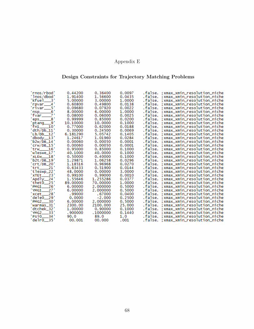
Appendix E

Design Constraints for Trajectory Matching Problems

68

Appendix F

Modified ACO Algorithm Source Code

Questions and requests for full programs can be sent to : [email protected]

Simple Matlab Program to find the Minimum Value of a Function of Two

Variables:

%ACO Mod

%Zachary Kiyak

%14 May 2013

% This program uses the ACO−Mod a lgor i thm to f i nd the minimum va lue

% of the s i x−humped camelback func t i on over the range x [−5 ,5] & y [−5 ,5]

clc ;

clear a l l

close a l l

runtype = 2 ; % runtype − 1 combines q parameter we i gh t ing wi th

% qmod e l i t i sm // runtype − 2 turns o f f q we i gh t ing

Ncycles = 5 ;

sigma = 0 . 5 ; % i n i t i a l s tandard d e v i a t i on used f o r r e s e t t i n g s o l u t i o n arch i v e

%Set Parameters

69

k = 20 ; % s i z e o f s o l u t i o n arch i v e

nv = 2 ; % number o f v a r i a b l e s

ni = 500 ; %number o f i t e r a t i o n s /mini−c y c l e

m = 2 ; % number o f new ants / c y c l e

q = 0 . 5 ; % weigh t ing parameter

eta = 0 . 7 ; % pheromone d i s t r i b u t i o n parameter

qmod = 0 . 4 ; % e l i t i sm parameter

%Store a l gor i thm parameters in vec t o r

paramset (1 ) = k ;

paramset (2 ) = nv ;

paramset (3 ) = m;

paramset (4 ) = q ;

paramset (5 ) = eta ;

% Set v a r i a b l e l im i t s

L(1) = −5;

L(2 ) = −5;

U(1) = −L ( 1 ) ;

U(2) = −L ( 2 ) ;

% Create Boundary Vector

for i = 1 : nv

B( i , 1 ) = L( i ) ;

70

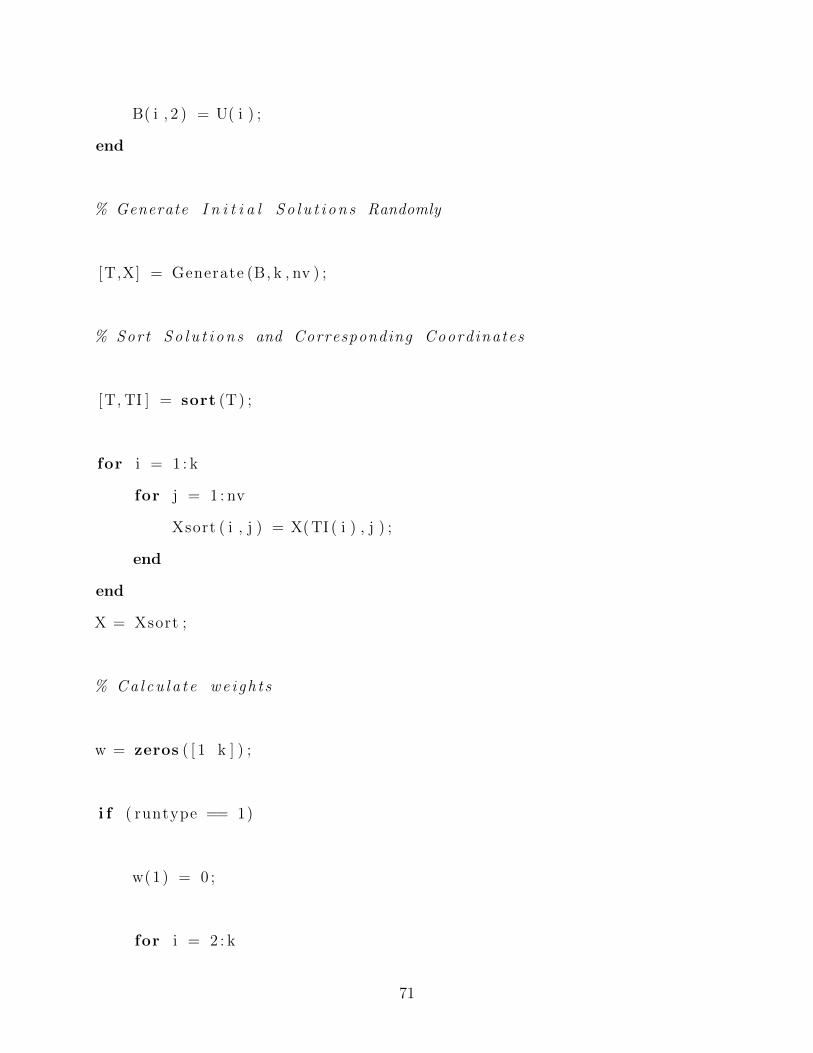
B( i , 2 ) = U( i ) ;

end

% Generate I n i t i a l So l u t i on s Randomly

[T,X] = Generate (B, k , nv ) ;

% Sort So l u t i on s and Corresponding Coordinates

[T, TI ] = sort (T) ;

for i = 1 : k

for j = 1 : nv

Xsort ( i , j ) = X( TI ( i ) , j ) ;

end

end

X = Xsort ;

% Ca l cu l a t e we i gh t s

w = zeros ( [ 1 k ] ) ;

i f ( runtype == 1)

w(1) = 0 ;

for i = 2 : k

71

rank = i ;

wden = q∗k∗sqrt (2∗pi ) ;

wnum = exp(−((rank−1)ˆ2)/(2∗qˆ2∗k ˆ 2 ) ) ;

w( i ) = wnum/wden ;

end

wsum = sum(w) ;

end

% Ca l cu l a t e P r o b a b i l i t i e s

P = zeros ( [ 1 k ] ) ;

i f ( runtype == 1)

P(1) = qmod ;

for i = 2 : k

P( i ) = (w( i )/wsum)∗(1−qmod ) ;

end

end

i f ( runtype == 2)

P(1) = qmod ;

72

for i = 2 : k

P( i ) = (1−qmod)∗ (1/ ( k−1)) ;

end

end

for i i = 1 : n i

[T X] = AntCycleMod (T,X,P, paramset ,B) ;

end

[ best , b i ] = min(T) ;

for j j = 1 : Ncyc les

% Generate Rebel Ant So lu t i on Archive

[ TReb , XReb ] = Generate (B, k , nv ) ;

% Sort So l u t i on s and Corresponding Coordinates

[ TReb , TI ] = sort (TReb ) ;

for i = 1 : k

for j = 1 : nv

Xsort ( i , j ) = XReb( TI ( i ) , j ) ;

73

end

end

XReb = Xsort ;

% Run Optimizer f o r Rebel Ant Colony

for i i = 1 : n i

[ TReb XReb ] = AntCycleMod (TReb , XReb ,P, paramset ,B) ;

end

[ bestreb , b i r eb ] = min(TReb ) ;

% Compare Best So lu t i on wi th t ha t Found by Main Colony

% I f Better , Replace

i f ( be s t r eb < best )

best = bes t r eb ;

X = XReb ;

b i = b i r eb ;

end

% Permute New So lu t i on Archive Around Best Coordinates

for i = 1 : k

i f ( i ˜= bi )

74

for j = 1 : nv

X( i , j ) = X( j , b i ) + normrnd (X( j , b i ) , sigma )∗ (B( j ,2)−B( j , 1 ) ) ;

end

end

T( i ) = camelback (X( i , 1 ) ,X( i , 2 ) ) ;

end

[T TI ] = sort (T) ;

for i = 1 : k

for j = 1 : nv

Xsort ( i , j ) = X( TI ( i ) , j ) ;

end

end

X = Xsort ;

% Run Optimizer on Re−d i s t r i b u t e d So lu t i on Archive

for i i = 1 : n i

[T X] = AntCycleMod (T,X,P, paramset ,B) ;

end

[ best , b i ] = min(T) ;

sigma = sigma − ( 0 . 4/ Ncycles ) ;

end

75

bestx = X( bi , 1 ) ;

besty = X( bi , 2 ) ;

t rue = −1.0316284534898774; %known minimum va lue

fpr intf ( ’\nThe Minimum Function Value I s : \n%4.16 f \n ’ , bes t )

fpr intf ( ’\nThe Corresponding X Coordinate I s : \n%4.10 f \n ’ , bestx )

fpr intf ( ’\nThe Corresponding Y Coordinate I s : \n%4.10 f \n ’ , besty )

fpr intf ( ’\nThe Error I s : \n%4.10 e\n ’ ,abs ( best−t rue ) )

///////////////////////////////////////////////////////////////////////////////

function [ Archive , Coords ] = AntCycleMod ( IArchive , ICoords , IProbs , Params , Lims )

P = IProbs ;

% Ca l cu l a t e P r o b a b i l i t i e s

k = Params ( 1 ) ;

nv = Params ( 2 ) ;

m = Params ( 3 ) ;

q = Params ( 4 ) ;

eta = Params ( 5 ) ;

Coords = ICoords ;

Archive = IArchive ;

76

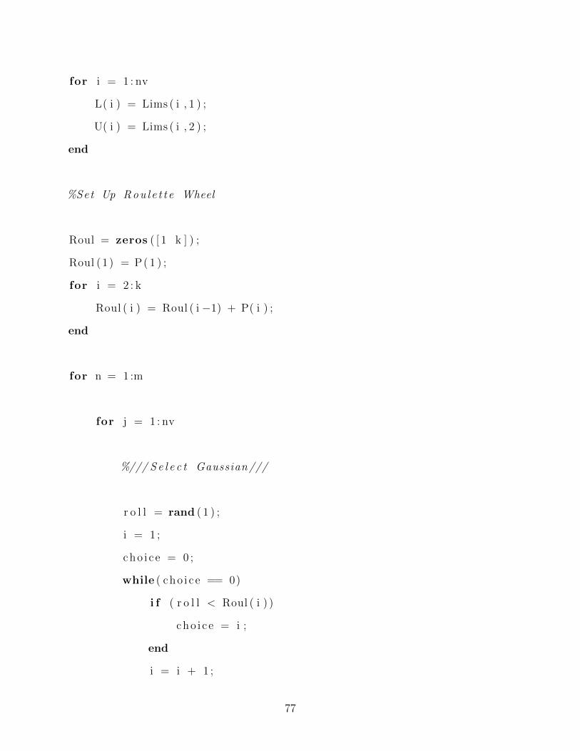
for i = 1 : nv

L( i ) = Lims ( i , 1 ) ;

U( i ) = Lims ( i , 2 ) ;

end

%Set Up Rou l e t t e Wheel

Roul = zeros ( [ 1 k ] ) ;

Roul (1 ) = P( 1 ) ;

for i = 2 : k

Roul ( i ) = Roul ( i −1) + P( i ) ;

end

for n = 1 :m

for j = 1 : nv

%/// S e l e c t Gaussian ///

r o l l = rand ( 1 ) ;

i = 1 ;

cho i c e = 0 ;

while ( cho i c e == 0)

i f ( r o l l < Roul ( i ) )

cho i c e = i ;

end

i = i + 1 ;

77

end

%///Sample Gaussian ///

% Ca l cu l a t e Sigma

for mm = 1 : k

s i g v e c (mm) = abs ( Coords ( cho ice , j )−Coords (mm, j ) ) ;

end

sigma = eta ∗ ( (sum( s i g v e c ) ) / ( k−1)) ;

% Take Sample

Xsam( j , n ) = normrnd ( Coords ( cho ice , j ) , sigma ) ;

% Enforce Limits

i f (Xsam( j , n)<L( j ) )

Xsam( j , n ) = L( j ) ;

end

i f (Xsam( j , n)>U( j ) )

Xsam( j , n ) = U( j ) ;

end

end

% Construct New So l u t i on s

78

Tsam(n) = camelback (Xsam(1 , n ) ,Xsam(2 , n ) ) ;

end

% Replace worst s o l u t i o n s

for i = 1 :m

Archive ( k+1− i )=Tsam( i ) ;

for j = 1 : nv

Coords ( k+1−i , j ) = Xsam( j , i ) ;

end

end

[ Archive , TI ] = sort ( Archive ) ;

for i = 1 : k

for j = 1 : nv

Xsort ( i , j ) = Coords ( TI ( i ) , j ) ;

end

end

Coords = Xsort ;

end

//////////////////////////////////////////////////////

79

function [ Values , Coords ] = Generate ( Bounds , Number , Dimensions )

L = Bounds ( : , 1 ) ;

U = Bounds ( : , 2 ) ;

% Generate I n i t i a l So l u t i on s Randomly

Coords = zeros ( [ Number Dimensions ] ) ;

for i = 1 : Number

for j = 1 : Dimensions

Coords ( i , j ) = L( j )+(U( j )−L( j ) )∗ rand ( 1 ) ;

end

end

% Evaluate I n i t i a l So l u t i on s

Values = zeros ( [ 1 Number ] ) ;

for i = 1 : Number

Values ( i ) = camelback ( Coords ( i , 1 ) , Coords ( i , 2 ) ) ;

end

80

Ant Colony Optimization: An Alternative Heuristic for ...

Documents

Transcript of Ant Colony Optimization: An Alternative Heuristic for ...