Ant Colony Algorithms and its applications to Autonomous...
88
IN DEGREE PROJECT MATHEMATICS, SECOND CYCLE, 30 CREDITS , STOCKHOLM SWEDEN 2017 Ant Colony Algorithms and its applications to Autonomous Agents Systems DANIEL JARNE ORNIA KTH ROYAL INSTITUTE OF TECHNOLOGY SCHOOL OF ENGINEERING SCIENCES
Transcript of Ant Colony Algorithms and its applications to Autonomous...

IN DEGREE PROJECT MATHEMATICS,SECOND CYCLE, 30 CREDITS
, STOCKHOLM SWEDEN 2017
Ant Colony Algorithms and its applications to Autonomous Agents Systems
DANIEL JARNE ORNIA
KTH ROYAL INSTITUTE OF TECHNOLOGYSCHOOL OF ENGINEERING SCIENCES


Ant Colony Algorithms and its applications to Autonomous Agents Systems DANIEL JARNE ORNIA Degree Projects Systems Engineering (30 ECTS credits) Degree Programme in Aerospace Engineering (120 credits) KTH Royal Institute of Technology year 2017 Supervisor at TU Delft: Manuel Mazo Supervisor at KTH: Xiaoming Hu Examiner at KTH: Xiaoming Hu

TRITA-MAT-E 2017:74 ISRN-KTH/MAT/E--17/74--SE Royal Institute of Technology School of Engineering Sciences KTH SCI SE-100 44 Stockholm, Sweden URL: www.kth.se/sci

Abstract I
Med den senaste tidens utveckling inom autonoma agentsystem och teknologier, finns ett okat
intresse for utveckling av styralgoritmer och metoder for att koordinera stora mangder roboten-
heter. Inom detta omrade visar anvandandet av biologiskt inspirerade algoritmer, baserade pa
naturliga svarmbeteenden, intressanta egenskaper som kan utnyttjas i styrandet av system som
innefattar ett flertal agenter. Dessa ar uppbyggda av simpla instruktioner och kommunikation-
smedel for att tillgodose struktur i systemet.
I synnerhet fokuserar detta masterexamensarbete pa studier av Ant Colony-algoritmer, baser-
ade pa stigmergy-interaktion for att koordinera enheter och fa dem att utfora specifika uppgifter.
Den forsta delen behandlar den teoretiska bakgrunden och konvergensbevis medan den andra
delen i huvudsak bestar av experimentella simuleringar samt resultat. Till detta andamal har
metriska parametrar utvecklats, vilka ansags sarskilt anvandbara nar planeringen av en enkel
bana studerades. Huvudkonceptet som utvecklats i detta arbete ar en tillampning av Shannon-
Entropi, vilket mater enhetlighet och ordning i ett system samt den viktade grafen. Denna
parameter har anvants for att studera prestandan och resultaten hos ett autonomt agentsys-
tem baserat pa Ant Colony-algoritmer.
Slutligen har denna styralgoritm modifierats for att utveckla ett handelsestyrt styrschema.
Genom att anvanda egenskaperna hos den viktade grafen (entropi) tillsammans med sensorsys-
temet hos agentenheterna, sa har en decentraliserad handelsestyrd metod implementerats, tes-
tats och visat sig ge okad effektivitet gallande utnyttjandet av systemresurser.
i

ii
Abstract II
With the latest advancements in autonomous agents systems and technology, there is a growing
interest in developing control algorithms and methods to coordinate large numbers of robotic
entities. Following this line of work, the use of biologically inspired algorithms based on swarm
emerging behaviour presents some really interesting properties for controlling multiple agents.
They rely on very simple instructions and communications to develop a coordinated structure
in the system.
Particularly, this master thesis focuses on the study of Ant Colony algorithms based on stig-
mergy interaction to coordinate agents and perform a certain task. The first part focuses on
the theoretical background and algorithm convergence proof, while the second part consists of
experimental simulations and results. For this, some metric parameters have been developed
and found to be especially useful in the study of a simple path planning test case. The main
concept developed in this work is an adaptation of Shannon Entropy that measures uniformity
and order in the system and the weighted graph. This parameter has been used to study the
performance and results of an autonomous agent system based on Ant Colony algorithms.
Finally, this control algorithm has been modified to develop an event-triggered control scheme.
Using the properties of the weighted graph (Entropy) and the sensing of the agents, a decentral-
ized event-triggered method has been implemented and tested, and has been found to increase
efficiency in the usage of system resources.
iii

iv

Acknowledgements
I would like to express my deepest gratitude first to Professor Manuel Mazo, who was more
than welcoming from the first moment and proposed me this project (that was in an extremely
early stage) when I first approached him. He guided me through the work and pushed me to
tackle the issues I was more reluctant to.
I want to thank as well the entire DCSC (Delft Center for Systems and Control) department
and TU Delft for having me and helping me out with anything I needed.
Also I thank Professor Xiaoming Hu from KTH for being my supervisor at my home university,
and the entire KTH institution not only for this work, but for the last years of studies that
exceeded the expectations (in every way) I had when I first got to Sweden two years ago.
Finally, I would like to thank my parents Sergio and Dolores for their support, their feedback
and second opinion whenever I sent them pieces of this work.
v

vi
Contents
Abstract I i
Abstract II i
Acknowledgements v
1 Introduction 1
1.1 Motivation and Concepts . . . . . . . . . . . . . . . . . . . . . . . . . . . . . . . 1
1.2 Goals and Expectations . . . . . . . . . . . . . . . . . . . . . . . . . . . . . . . 2
2 Background and Problem Description 3
2.1 Biological Inspiration and Background . . . . . . . . . . . . . . . . . . . . . . . 3
2.2 Event-Triggered Control . . . . . . . . . . . . . . . . . . . . . . . . . . . . . . . 4
2.3 Markov Process, Random Variables and Martingales . . . . . . . . . . . . . . . . 5
2.3.1 Markov Process . . . . . . . . . . . . . . . . . . . . . . . . . . . . . . . . 5
2.3.2 Martingales . . . . . . . . . . . . . . . . . . . . . . . . . . . . . . . . . . 5
2.4 Problem Description . . . . . . . . . . . . . . . . . . . . . . . . . . . . . . . . . 7
2.5 Dynamic System Model . . . . . . . . . . . . . . . . . . . . . . . . . . . . . . . 9
2.5.1 Solution Generation . . . . . . . . . . . . . . . . . . . . . . . . . . . . . 12
2.5.2 Pheromone Distribution . . . . . . . . . . . . . . . . . . . . . . . . . . . 14
2.5.3 Pheromone as a Random Variable . . . . . . . . . . . . . . . . . . . . . . 15
2.6 Entropy as a Metric Parameter . . . . . . . . . . . . . . . . . . . . . . . . . . . 18
vii
viii CONTENTS
2.6.1 Shannon Entropy . . . . . . . . . . . . . . . . . . . . . . . . . . . . . . . 18
2.6.2 Maximum and Minimum Entropy . . . . . . . . . . . . . . . . . . . . . . 19
2.6.3 Entropy Function and its Properties . . . . . . . . . . . . . . . . . . . . 21
2.6.4 Entropy Convergence . . . . . . . . . . . . . . . . . . . . . . . . . . . . . 23
2.7 Graph Convergence Criteria . . . . . . . . . . . . . . . . . . . . . . . . . . . . . 28
2.8 Entropy-Based Event Triggered Proposal . . . . . . . . . . . . . . . . . . . . . . 29
2.8.1 Proposal A: Entropy-Based Marking Frequency Shift . . . . . . . . . . . 29
2.8.2 Proposal B: Entropy Based Pheromone Intensity Shift . . . . . . . . . . 30
2.9 Decentralized Entropy Trigger . . . . . . . . . . . . . . . . . . . . . . . . . . . . 30
2.9.1 Surrounding Entropy Estimation . . . . . . . . . . . . . . . . . . . . . . 30
2.10 Summary of Concepts . . . . . . . . . . . . . . . . . . . . . . . . . . . . . . . . 32
3 Experimental Analysis and Results 33
3.1 Algorithm Implementation . . . . . . . . . . . . . . . . . . . . . . . . . . . . . . 33
3.2 Other Metric Parameters . . . . . . . . . . . . . . . . . . . . . . . . . . . . . . . 34
3.3 Convergence and Entropy Results . . . . . . . . . . . . . . . . . . . . . . . . . . 35
3.3.1 One and multiple optimal solutions . . . . . . . . . . . . . . . . . . . . . 35
3.3.2 Parametric convergence analysis . . . . . . . . . . . . . . . . . . . . . . . 41
3.3.3 Entropy Convergence . . . . . . . . . . . . . . . . . . . . . . . . . . . . . 44
3.4 Convergence Validation Experiments . . . . . . . . . . . . . . . . . . . . . . . . 47
3.5 Entropy-Based Event Triggered Control . . . . . . . . . . . . . . . . . . . . . . . 50
3.5.1 Proposal A: Results . . . . . . . . . . . . . . . . . . . . . . . . . . . . . . 50
3.5.2 Proposal B: Results . . . . . . . . . . . . . . . . . . . . . . . . . . . . . . 53
3.6 Decentralized Entropy Trigger: Results . . . . . . . . . . . . . . . . . . . . . . . 55
3.6.1 Entropy Estimation: Examples . . . . . . . . . . . . . . . . . . . . . . . 55
3.6.2 Decentralized Trigger - Proposal B . . . . . . . . . . . . . . . . . . . . . 57
3.6.3 Decentralized Trigger Results . . . . . . . . . . . . . . . . . . . . . . . . 59

4 Conclusion 62
4.1 Summary of Results . . . . . . . . . . . . . . . . . . . . . . . . . . . . . . . . . 62
4.2 Applications . . . . . . . . . . . . . . . . . . . . . . . . . . . . . . . . . . . . . . 64
4.3 Future Work . . . . . . . . . . . . . . . . . . . . . . . . . . . . . . . . . . . . . . 65
Bibliography 65
ix

x
List of Tables
3.1 Standard parameters for simulations . . . . . . . . . . . . . . . . . . . . . . . . 35
3.2 Maximum Pheromone Values . . . . . . . . . . . . . . . . . . . . . . . . . . . . 35
3.3 Parameter results for simulation 1 . . . . . . . . . . . . . . . . . . . . . . . . . . 37
3.4 Entropy limit values for simulation 1 . . . . . . . . . . . . . . . . . . . . . . . . 38
3.5 Parameters for simulation 2 . . . . . . . . . . . . . . . . . . . . . . . . . . . . . 38
3.6 Maximum Pheromone Values 2 . . . . . . . . . . . . . . . . . . . . . . . . . . . 38
3.7 Parameter results for simulation 2 . . . . . . . . . . . . . . . . . . . . . . . . . . 39
3.8 Entropy limit values for simulation 2 . . . . . . . . . . . . . . . . . . . . . . . . 39
3.9 Parameters for Convergence Experiments . . . . . . . . . . . . . . . . . . . . . . 41
3.10 Experiment Results for nants = 15 . . . . . . . . . . . . . . . . . . . . . . . . . . 41
3.11 Experiment Results for ρ = 0.03 . . . . . . . . . . . . . . . . . . . . . . . . . . . 43
3.12 Parameters for Proposal A . . . . . . . . . . . . . . . . . . . . . . . . . . . . . . 50
3.13 Cycle Parameter Values . . . . . . . . . . . . . . . . . . . . . . . . . . . . . . . 51
3.14 Total amount of Pheromones added . . . . . . . . . . . . . . . . . . . . . . . . . 52
3.15 Parameters for Decentralised Event Triggered Simulations . . . . . . . . . . . . 59
3.16 Results for standard simulations . . . . . . . . . . . . . . . . . . . . . . . . . . . 59
3.17 Results for different slopes . . . . . . . . . . . . . . . . . . . . . . . . . . . . . . 60
xi

xii
List of Figures
2.1 Grid Structure . . . . . . . . . . . . . . . . . . . . . . . . . . . . . . . . . . . . 9
2.2 Agent walking between nodes . . . . . . . . . . . . . . . . . . . . . . . . . . . . 14
2.3 Agent Neighbourhood . . . . . . . . . . . . . . . . . . . . . . . . . . . . . . . . 30
3.1 Pheromone Graph evolution . . . . . . . . . . . . . . . . . . . . . . . . . . . . . 36
3.2 Entropy Results for simulation 1 . . . . . . . . . . . . . . . . . . . . . . . . . . . 37
3.3 Pheromone Graph evolution . . . . . . . . . . . . . . . . . . . . . . . . . . . . . 39
3.4 Entropy Results for simulation 2 . . . . . . . . . . . . . . . . . . . . . . . . . . . 40
3.5 Entropy Results for variable evaporation . . . . . . . . . . . . . . . . . . . . . . 42
3.6 Entropy Results for variable number of agents . . . . . . . . . . . . . . . . . . . 43
3.7 Convergence in Entropy . . . . . . . . . . . . . . . . . . . . . . . . . . . . . . . 44
3.8 Convergence to Optimal Solution . . . . . . . . . . . . . . . . . . . . . . . . . . 45
3.9 Entropy at 1500s . . . . . . . . . . . . . . . . . . . . . . . . . . . . . . . . . . . 46
3.10 Time plot of γ for all nodes . . . . . . . . . . . . . . . . . . . . . . . . . . . . . 47
3.11 Time plot of γ ∈ (0, 5) for all nodes . . . . . . . . . . . . . . . . . . . . . . . . . 48
3.12 Time plot of γ . . . . . . . . . . . . . . . . . . . . . . . . . . . . . . . . . . . . . 49
3.13 Entropy Computation and Entropy Limit Example . . . . . . . . . . . . . . . . 50
3.14 Entropy for Event Triggered and Continuous Marking . . . . . . . . . . . . . . . 51
3.15 Quadratic Event Trigger . . . . . . . . . . . . . . . . . . . . . . . . . . . . . . . 52
3.16 Results for z=1/1000 . . . . . . . . . . . . . . . . . . . . . . . . . . . . . . . . . 53
xiii
3.17 Results for z=1/800 trigger slope . . . . . . . . . . . . . . . . . . . . . . . . . . 54
3.18 Entropy for Intensity Trigger . . . . . . . . . . . . . . . . . . . . . . . . . . . . . 54
3.19 Global Entropy and Entropy Estimations . . . . . . . . . . . . . . . . . . . . . . 55
3.20 Average Estimated Entropy and Real Time Entropy . . . . . . . . . . . . . . . . 56
3.21 Entropy Results for Linear Threshold . . . . . . . . . . . . . . . . . . . . . . . . 57
3.22 Entropy Results for Quadratic Threshold . . . . . . . . . . . . . . . . . . . . . . 58
3.23 Entropy Results for several slopes . . . . . . . . . . . . . . . . . . . . . . . . . . 60
3.24 Cycle Parameter for Decentralized Simulations . . . . . . . . . . . . . . . . . . . 61
3.25 Convergence Time and Pheromone Efficiency . . . . . . . . . . . . . . . . . . . . 61
xiv
Chapter 1
Introduction
1.1 Motivation and Concepts
In the past couple of decades there has been a growing interest in the systems engineering and
control field to apply computer science concepts and algorithms to engineering problems. From
biologically inspired optimization algorithms to AI and deep learning methods, these tools are
being currently applied to engineering fields such as robotics, transport automation and so on.
The concept of Swarm Intelligence comes from putting together biologically inspired algorithm
with machine learning techniques. It is an analogous idea to Artificial Intelligence; while AI
focuses on having a highly complex system learn to perform highly complex tasks, SI is based
on the idea of having several extremely simple agents or systems learning to perform a complex
task or solve a complex problem by collective emerging behaviour methods. This is why Swarm
Intelligence uses (in many of its forms and applications) biologically inspired systems and
algorithms; nature is full of swarm behaviour examples, from bee hives and ant nests to fish
schools and bird flocks.
Parallel to this, event-triggered control focuses on the active scheduling of control tasks in a
system. Instead of periodic feedback between sensors, processors and actuators, event-triggered
methods focus on defining threshold conditions for each subsystem, so that the control tasks
can be scheduled independently depending on some desired triggering function, greatly reducing
network loads, increasing battery life, etc. This method also enables us to decentralize control
tasks, enabling each set of sensors and actuators to act independently of a central processing
system.
The idea is that emerging behaviour algorithms, and in general most algorithms that go through
some kind of learning process, are usually considered to be a ”black box”. It becomes extremely
1

2 Chapter 1. Introduction
hard to understand the process that develops inside, and it is even harder to tune and modify
the behaviour of the algorithm to obtain different performances. Through the analysis and
application of the metrics we can better understand the process that goes on when the system
is evolving from a uniform and chaotic state to a coordinated and structured behaviour.
Following this line of thought, the work in this thesis will be focused on ant inspired behaviour
applied to autonomous agent systems. In this case Ant Algorithms that have been for long
applied to discrete optimization problems can be used to control a physical system of simple
agents (robots, drones, etc...), focusing on a simple path planning robotic problem. To study
these methods and have some validation, some metric concepts will be developed and a deeper
mathematical reasoning will be laid out in order to argue and justify the validity of the work.
1.2 Goals and Expectations
The main goals in this work will be related to the two lines of study mentioned before; Event-
Triggered Control and Swarm Intelligence. Hence, we can summarize the goals and expected
outcomes:
• Study and develop new methods and metrics for analyzing Swarm Intelligence Algorithms,
applied in particular to Ant Colony Algorithms, to further understand and represent the
behaviour and evolution process for these algorithms.
• Develop a control routine based on this algorithm for a path planning system of multi-
agents.
• Analyze the impact that the problem parameters have on the convergence and behaviour
of the system.
• Suggest and implement solutions and schemes for turning the algorithm into an event-
based triggered system, relating the coordination of the agents to the interaction with
the environment (pheromone marking).
• Explore ways to decentralize the control tasks, so each agent can act independently.
Finally, the work will first be focused on theoretical and simulated environments, leaving the
practical implementation for further work depending on the resources available.

Chapter 2
Background and Problem Description
In order to understand the emerging behavior in the proposed set of autonomous agents through
an ant inspired algorithm, first we will cover the background and specific characteristics of
ant optimisation algorithms, and how they can be used to implement a control system for a
swarm of autonomous agents. Then the specific problem to be solved is described, as well as
the computational implementation of the algorithms for this particular problem. Also, some
concepts such as Entropy and Martingale Theory are presented for further use in the algorithm
convergence and performance analysis.
2.1 Biological Inspiration and Background
In the past years there has been a growing interest in biologically-inspired algorithms for solving
a wide range of different problems. Ant colony algorithms, formally described first by M. Dorigo
([1], [2]) are a kind of insect inspired algorithms which (like bee-hive algorithms, etc) rely on
emerging behaviour from a big group of simple agents.
In the case of ant algorithms, they are very much based on ant foraging behaviour ([3]). The
biological process that ants follow when foraging to find the shortest path to the food source
is called Stigmergy. The concept of Stigmergy is based on independent agents communicating
through environment interaction. Ants do this by leaving a trail of pheromones when looking
for food. Once the food is found, ants head back to the nest adjusting the pheromone marking
depending on food quality, etc. The implicit idea behind this behaviour is that since pheromones
evaporate with time, shorter paths will have on average a higher amount of pheromones. Other
ants then follow these pheromone trails, probabilistically choosing the ones with a bigger amount
of pheromones. Eventually, only ”short” paths prevail, hence reaching an optimal solution and
having most ants travelling through the shortest path.
Examples of ant inspired algorithms can be found for solving a wide range of optimization
3
4 Chapter 2. Background and Problem Description
problems (see references [4] and [5]). The idea in this case is to modify these algorithms to be
apply them to control a swarm of autonomous agents, getting them to perform a certain task
in a coordinated way. Focusing first on ant foraging, these algorithms can be implemented so
that the ants walking around the domain are thought of as a swarm of autonomous agents.
The algorithm then enables the swarm to eventually converge to a certain organized solution,
starting from a chaos dominated behaviour. This would set the ground for applying these
methods as an event-triggered controller, where the swarm interacts with the environment
depending on the level of chaos or coordination required.
After the literature research process, a gap was noticed in the previous work done in this
field. There is extensive research in using Ant Colony Algorithms to solve discrete optimization
problems. In fact, this was the first use of these algorithms since M. Dorigo ([1]) first introduced
them. Lately, these methods have been explored in practical applications (see [6], [7] and [8]).
This has raised some questions on how complex the agents have to be, and how big must the
surrounding and monitoring system be in order to obtain the desired optimal motion. This
means that, in many cases, the algorithms have to be adapted to comply with the physical and
equipment limitations of the robotic agents.
This is one of the main differences between the version of the ant algorithm developed in this
work and other used in previous optimization problems (see [4]). In this case, the final goal of
the algorithm is to be implemented as a control method for an autonomous multi-agent (swarm)
system. Hence, the algorithm description is focused not on quality or speed of convergence for
this particular optimization problem, but on practicalities when applying this scheme to swarm
coordination and behavior of robotic systems.
The goal of this work is then to propose a continuous form of the algorithm that enables agents
to use it as a control routine, while keeping the resource requirements to the minimum. Also,
try to gain a deeper understanding of these methods, keeping in mind possible future practical
applications and implementations in physical systems.
2.2 Event-Triggered Control
Control tasks in a sensor/actuator system are usually time-triggered; that means the system
checks periodically the sensor signal, and executes the control tasks accordingly. The idea of
event-triggered control is to schedule the control tasks according to the feedback on the sensors,
so that the actuators work only when the signal goes above a desired threshold. So in this case,
the control tasks are triggered by certain ”events”, instead of being scheduled periodically. This
optimizes resources in the system, by taking a more efficient approach to scheduling the control
tasks (for a more detailed description of event-triggered control and its benefits, see [9]).
In our case, this idea can be extended to the ant system. Seeing the environment marking
2.3. Markov Process, Random Variables and Martingales 5
(pheromones) as a control task through which the system seeks a stabilization or convergence,
the standard functioning would be the equivalent to periodic time control. The agents mark
at each time step depending on the type of algorithm. The idea is then to design some kind
of event-triggering function that lets the agents schedule the control tasks more efficiently. So
instead of interacting continuously with the environment (and hence each other) the agents
will only do so when the system goes past a certain limit (triggering) condition. Finding and
applying this condition is hence one of the goals of the work presented here. For this, the
concept of entropy is presented in section 2.6.
2.3 Markov Process, Random Variables and Martingales
In order to study the behaviour of the algorithm and to make sure the modifications to be
introduced in the system are valid, some proof of convergence needs to be developed. For that
we will make use of random variable and probabilistic theory tools such as the concepts of
Markov Process and Martingale.
2.3.1 Markov Process
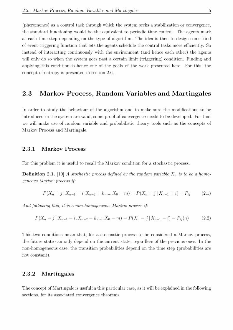
For this problem it is useful to recall the Markov condition for a stochastic process.
Definition 2.1. [10] A stochastic process defined by the random variable Xn is to be a homo-
geneous Markov process if:
P (Xn = j |Xn−1 = i,Xn−2 = k, ..., X0 = m) = P (Xn = j |Xn−1 = i) = Pij (2.1)
And following this, it is a non-homogeneous Markov process if:
P (Xn = j |Xn−1 = i,Xn−2 = k, ..., X0 = m) = P (Xn = j |Xn−1 = i) = Pij(n) (2.2)
This two conditions mean that, for a stochastic process to be considered a Markov process,
the future state can only depend on the current state, regardless of the previous ones. In the
non-homogeneous case, the transition probabilities depend on the time step (probabilities are
not constant).
2.3.2 Martingales
The concept of Martingale is useful in this particular case, as it will be explained in the following
sections, for its associated convergence theorems.
6 Chapter 2. Background and Problem Description
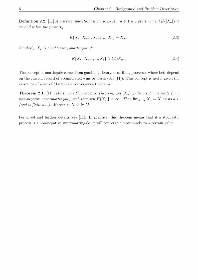
Definition 2.2. [11] A discrete time stochastic process Xn, n > 1 is a Martingale if E{|Xn|} <∞ and it has the property:
E{Xn |Xn−1, Xn−2, ..., X1} = Xn−1 (2.3)
Similarly, Xn is a sub(super)-martingale if:
E{Xn |Xn−1, ..., X1} > (6)Xn−1 (2.4)
The concept of martingale comes from gambling theory, describing processes where bets depend
on the current record of accumulated wins or losses (See [11]). This concept is useful given the
existence of a set of Martingale convergence theorems.
Theorem 2.1. [11] (Martingale Convergence Theorem) Let (Xn)n>1 be a submartingale (or a
non-negative supermartingale) such that supnE{X+n } < ∞. Then limn→∞Xn = X exists a.s.
(and is finite a.s.). Moreover, X is in L1.
For proof and further details, see [11]. In practice, this theorem means that if a stochastic
process is a non-negative supermartingale, it will converge almost surely to a certain value.
2.4. Problem Description 7
2.4 Problem Description
Overall, the idea behind this method is to achieve coordination in a set of autonomous agents
interacting with each other through the environment. This can be structured as a discrete
optimization problem, assuming there is a finite set of solutions and the agents walk the graph
trying to find the optimal ones. The behaviour of the process can be described by a dynamic
system model and as a random variable.
Consider an optimization problem described by the graph G = (V ,L,W), which consists of
a set of vertex V , a set of links between vertex L, and a set of weights (pheromone values)
W = f(t) associated to the links L.
One of the main differences with other optimization problems is that in this case the weight
field is part of the graph description but also part of the solution; solutions are constructed
increasing pheromones on the desired links, starting at initial node pi and finishing at node pf .
The optimization problem to solve is a path planning or routing problem. Hence, the problem
is defined by (S, g), where :
• S is a set of all feasible solutions with |S| < ∞ defined in terms of node sequences s so
that s = {vi, ..., vk, ..., vf} and they fulfill the conditions:
– vi = pi and vf = pf .
– ls(k),s(k+1) ∈ L ∀ k ∈ [1, |s| − 1].
• g(s) is a cost function, g : S → R>0.
It is assumed that a set S∗ ⊆ S of optimal solutions exists, and it is defined:
g(s∗) = min{g(si)} , ∀i ∈ [1, 2, ...|S|] (2.5)
The problem then consists on finding at least one of the solutions that fulfill condition 2.5 in a
finite amount of time. This is done by a number of agents N that walk the graph stochastically
constructing possible solutions, i.e. reaching the goal node having started from the initial node,
while following a set of plausible links connecting the visited nodes. In this case, focusing first
on a simple implementation, the graph G will be represented by a two-dimensional grid.
Each agent will follow a probabilistic model to construct a possible solution formed by a set of
solution components, which in this case are the subsequent set of links L′ ⊆ L connecting the
set of visited nodes P ′. Between two interconnected nodes (vi, vj) (i.e. for a given link lij ∈ L),
there is an assigned value τij of pheromones associated to that link. Hence, for each time step,
agents choose probabilistically between the connected nearby nodes following these pheromone
trails.
8 Chapter 2. Background and Problem Description
Agents then deposit a certain amount ∆τ on the links between walked nodes after each time
step. These pheromones have (as in real ant behavior) a certain evaporation factor ρ associated.
Hence, after every time step, the pheromones on the graph are updated by both the movement
of the agents and the evaporation of the pheromones. In this case the evaporation acts as a
form of implicit cost function; longer solutions will take more time to be completed, so the
pheromones decrease further compared to those shorter paths with a faster completion time.
Considering this, the cost function g(s) cannot be computed explicitly and used to actively
affect the behavior of the algorithm after each step. In other ant-inspired algorithms explicit
cost functions (such as path length, time cost, etc) are used to evaluate the quality of the
solutions that are being generated, and then adjust the pheromone values accordingly. In
this case, the pheromones are thought of as a physical trail or mark in the environment left
behind by an agent when moving. Since memory and information sharing is to be kept to
the minimum in each agent, and the idea is to build an algorithm as generalist as possible
(applicable to different kinds of physical systems) that relies on swarm coordination rather
than agent computing capabilities and precision, having this implicit cost function may (and
probably will) slow down the convergence, but it is a much more permissive method regarding
physical implementation.
2.5. Dynamic System Model 9
2.5 Dynamic System Model
We can now model the problem as a discrete time dynamic system. First, let us define the
adjacency matrix for this weighted graph A, |V| × |V| size, such that:
Aij = 1 , ∀i, j : ∃ lij ∈ LAij = 0 else.
The values of Aij are then related to the existence of a valid link between nodes i and j. In
other words, if node i is connected to node j in the graph, Aij = 1. So, in this case, the diagonal
terms of the matrix Aii represent the possibility of enabling agents to stay in the node they are
in. Since for our problem this is not required, it will be set Aii = 0 for all i, so that agents are
not allowed to stay in the same node on consecutive time steps.
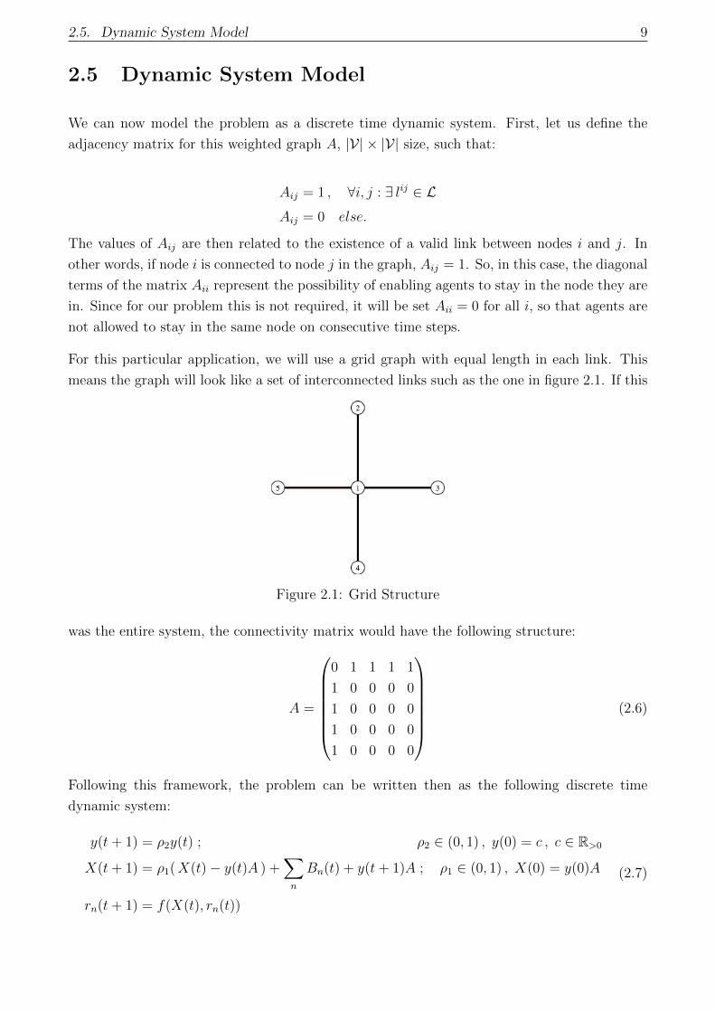
For this particular application, we will use a grid graph with equal length in each link. This
means the graph will look like a set of interconnected links such as the one in figure 2.1. If this
Figure 2.1: Grid Structure
was the entire system, the connectivity matrix would have the following structure:
A =
0 1 1 1 1
1 0 0 0 0
1 0 0 0 0
1 0 0 0 0
1 0 0 0 0
(2.6)
Following this framework, the problem can be written then as the following discrete time
dynamic system:
y(t+ 1) = ρ2y(t) ; ρ2 ∈ (0, 1) , y(0) = c , c ∈ R>0
X(t+ 1) = ρ1(X(t)− y(t)A ) +∑n
Bn(t) + y(t+ 1)A ; ρ1 ∈ (0, 1) , X(0) = y(0)A
rn(t+ 1) = f(X(t), rn(t))
(2.7)
10 Chapter 2. Background and Problem Description
In the system described, y(t) is a ”virtual” (it is not added by the agents) base pheromone value
with an assigned specific evaporation rate ρ2 and initial value c. This is introduced so that the
graph is initially explorable for all ants, without the need of real pheromone spreading, with
ρ1 being the real pheromone evaporation rate. The state variables X(t) and rn(t) represent
the amount of pheromones in each link and the position of the agents. According to the graph
description:
X(t) ≡ W(t) , Xij(t) = τij(t)
In this way, we make sure that pheromones are only added to valid links in the graph, and
enables us (together with the artificial pheromones y(t)) to write the probability law in a very
simple form. Finally, Bn is a stochastic (random) coefficient |V|× |V| matrix that only depends
on the current state X(t) generated by agent n in every step. This represents the pheromone
increase function, and it has the values:
Bn,ij(t) = ∆τ , ∀i, j : {rn(t+ 1) = j | rn(t) = i}Bn,ij(t) = 0 else.
Where rn(t) is the position in the graph of agent n at time t, which is a stochastic variable that
depends on the pheromone field. At last, the probability law for the agent steps is described
as:
P (rn(t+ 1) = j | rn(t) = i) =Xij(t)∑kXik(t)
, ∀k : ∃ lik ∈ L (2.8)
This means that the probability of an agent n moving from node i to node j is equal to the
pheromone value of link lij over the sum of pheromones for all possible links starting at node
i. Hence, the whole state of the system G is defined by the two variables:
G = f(X(t), rn(t)) (2.9)
Nevertheless, the variable rn(t) can be substituted by its inverse function, i.e. the amount of
agents in each node ai(t). This form becomes more useful when studying the evolution of the
graph, instead of individual agent positions.
We can now find a random variable that represents the system to study its properties. First,
we define the random variable Y as the pheromone distribution matrix X and the amount of
agents in each node ai(t):
Y (t) =
a1(t)
X(t) ...
a|V|(t)
(2.10)
Hence, our problem can be written as a random variable, and the expected value for a given
time t+ 1 only depends on the variable values at t.
2.5. Dynamic System Model 11
Proposition 2.1. The ant algorithm dynamic system described in 2.4 is a non-homogeneous
Markov Process defined by the random variable Y (t).
Proof. Consider first the pheromone field X(t). In each time step, the values Xij(t) can only
change through two different mechanisms; evaporation and pheromone addition. Hence, the
probability for the values Xij(t+ 1) is:
P{Xij(t+ 1) = ρXij(t) + ki∆τ} =
(Xij(t)∑|V|k=1Xik(t)
)ki
∀ ki ∈ [0, 1, ..., ai(t)] (2.11)
In this case ki is an integer value that represents the different possible states (amount of agents
crossing the path). As it can be seen, the pheromone field is a non-homogeneous Markov
process. Finally, for the value of ai(t):
P{ai(t+ 1) = qi} = f(X(t), aNi (t)) (2.12)
Where aNi (t) is the amount of agents in the neighbourhood of i. This is easy to see when
considering that the position of the agents rn(t) only depend on the pheromone field at time t
(expression 2.8). With X(t) and ai(t) i, the variable Y (t) is defined.
Proposition 2.2. The expected conditional value of the random variable E{Y (t+ 1) |H} only
depends on the values of the variable at time t, i.e:
E{Y (t+ 1) |Y (t)} = E{Y (t+ 1) |Y (t), ..., Y (0)} = f(Y (t)).
Proof. Following the same notation as previously described, X(t) is our pheromone weight
graph. And in this case, ak is the amount of agents placed in node k at time t. Hence,
the variable Y has the size |V| × (|V| + 1). For simplicity in the expressions, we will define
M = |V| + 1. We can now write the expected conditional value for the variable Y , by first
recalling the probability of agents moving from i → j in expression 2.8. Hence, the expected
value of agents at j is:
E{aj(t+ 1) | a(t), X(t)} =
|V|∑l=1
al(t)Xlj(t)∑|V|k=1Xlk(t)
(2.13)
Since the pheromone trails between unconnected nodes are 0 by definition, we can write ex-
pression 2.13 as a sum for all nodes. Now, for the expected conditional value of Y we can use
the classic definition of E{Y (t + 1) |Y (t), ...Y (0)}. This means that the expected conditional
value of Y (t+1) is equal to the different possible outcomes of the variable times the probability
of those outcomes. For the case of the pheromones, it is then:
E{Xij(t+ 1) |Xij(t), ai(t)} = Xij(t)(1− ρ) + p∗ijai(t)∆τ
12 Chapter 2. Background and Problem Description
In this case, p∗ij represents the probability of agents traversing from i → j, and hence, using
2.8:
p∗ij =Xij∑|V|k=1Xik
Expression 2.13 means that the expected conditional value of agents at a certain node j and
time t+ 1 is equal to the amount of agents surrounding j times the probability of these agents
actually moving to j. It is interesting to see that this value does not depend on the current
amount of agents aj(t), since all the agents have to move for each time step. Also, note that
given the definition of the variable Y (t), we can write the number of agents a(t) in terms of Y :
ai(t) = YiM(t)
That is, the set of values contained in the last column of Y . With these expressions, and writing
everything in terms of the variable Y we get:
E{Y (t+ 1) |Y (t)} =
Yij(t)
((1− ρ) + YiM (t)∑|V|
k=1 Yik(t)∆τ)
, ∀ j ∈ [1, 2, ...|V|]
∑|V|k=1 Ykj(t)
Yki(t)∑|V|q=1 Ykq(t)
, j = |V|+ 1
(2.14)
Therefore, the expected value for Y (t+ 1) only depends on the current state Y (t).
2.5.1 Solution Generation
In order to fully define the behaviour of the system presented in (2.7), its relation to the
generation of valid solution must be described. First of all, the agents will store the amount
of steps N-S and E-W they take (two integer values) from the initial node until they reach the
goal node. We will introduce a kernel overlapping the pheromone field, such that:
Xij(t) = Xij(t) ·Qn if ∃t′ ≤ t : rn(t′) = vf (2.15)
Xij(t) = Xij(t) otherwise (2.16)
In condition (2.15), Qn is the kernel virtually modifying the surrounding weights given a certain
desired condition (i.e. the direction towards the nest) for a given agent n.
This kernel is the additional layer added to the algorithm in order to ensure a ”back-and-forth”
agent movement. Other options were considered, such as storing in each agent’s memory all the
followed steps until the goal node is reach, and then walking back that same path until the nest
is reached. The angular kernel was implemented due to a smaller amount of memory required
and the geometry of the problem to be solved. In any case, this additional algorithm layer
must be implemented to impose the desired behaviour conditions to be met, i.e. a recurrent
walk between goal and nest. Hence, in this case, the kernel is computed as follows:
2.5. Dynamic System Model 13
• Each agent stores two integer values, one for the amount of north-south (N-S) steps and
another one for east-west (E-W).
• When the goal is reached for the first time, an angle θf is computed using these values,
corresponding to the angular direction between goal and the nest. This angle is used
thereon to compare with the actual direction of the agent.
• From that point, the actual direction of the agent is compared after each step with the
angle θf , and the kernel Qn is computed accordingly.
In the first implementation, we will design this kernel with a simple angle relative difference:
Qn =|θn(t)− θf |
2π(2.17)
In this case, the angle differences are always computed in the closest arc. It must be noted
that the angle θn is the angle computed by the agent according to the N-S and E-W current
values, and it is relative to the previous limiting node encountered (goal or nest depending on
the cycle). Also, this kernel is designed in the most simple way considering the geometrical
problem.
This method causes that, after the initial exploration phase, the agents are ”pulled” into link se-
quences that start and end at the desired nodes. Then, the evaporation ensures the convergence
towards the shorter solution cycles.
14 Chapter 2. Background and Problem Description
2.5.2 Pheromone Distribution
The behavior of the algorithm must be described in a deeper way first, to better understand
the purpose and the results of the simulations and studies. Consider first a generic agent
constructing a solution following the procedure in expression 2.7. The agent will move between
interconnected nodes from the initial node to the final node in a stochastic way depending on
the pheromone value X between nodes. But for each step, the pheromone values are altered by
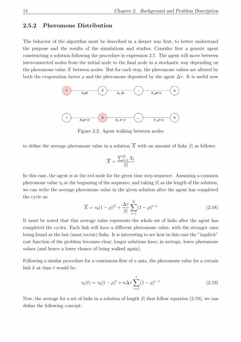
both the evaporation factor ρ and the pheromone deposited by the agent ∆τ . It is useful now
Figure 2.2: Agent walking between nodes
to define the average pheromone value in a solution X with an amount of links |l| as follows:
X =
∑|l|i=1 Xl
|l|
In this case, the agent is at the red node for the given time step sequence. Assuming a common
pheromone value τ0 at the beginning of the sequence, and taking |l| as the length of the solution,
we can write the average pheromone value in the given solution after the agent has completed
the cycle as:
X = τ0(1− ρ)|l| +∆τ
|l|
|l|∑i=1
(1− ρ)i−1 (2.18)
It must be noted that this average value represents the whole set of links after the agent has
completed the cycles. Each link will have a different pheromone value, with the stronger ones
being found at the last (most recent) links. It is interesting to see how in this case the ”implicit”
cost function of the problem becomes clear; longer solutions have, in average, lower pheromone
values (and hence a lower chance of being walked again).
Following a similar procedure for a continuous flow of n ants, the pheromone value for a certain
link k at time t would be:
τk(t) = τ0(1− ρ)t + n∆τt∑i=1
(1− ρ)i−1 (2.19)
Now, the average for a set of links in a solution of length |l| that follow equation (2.19), we can
define the following concept:
2.5. Dynamic System Model 15
Proposition 2.3. For a constantly walked solution (set of links), with a number of n agents
and an increment of pheromones ∆τ , the maximum value of average pheromones is:
τmax =n∆τ
ρ|l|(2.20)
Proof. Take expression (2.19), and consider a solution (set of links) l constantly walked in the
same manner. Taking the average pheromone value for this links:
X(t) =1
|l|∑k∈l
τk(t)
If there are n agents, we can consider they are split equally among links, so that we get n/|l|agents per link. Now taking the limit in time, we get the maximum value:
τmax = limt→∞
X(t) =1
|l|limt→∞|l|τ0(1− ρ)t + |l|n∆τ
|l|
t∑i=1
(1− ρ)i−1 =n∆τ
ρ|l|
This result is interesting because it gives us an upper bound to be expected in the frequently
walked solutions, i.e. the optimal solutions. This upper bound is then the maximum amount of
pheromones expected in the graph for the given parameters. The pheromones are then globally
bounded by τmax and τmin = 0.
2.5.3 Pheromone as a Random Variable
Now it is important to understand how these dynamics affect the pheromone field, considering
it to be a random variable (or a set of random variables).
Theorem 2.2. The pheromone values of links with agents on the nodes are sub-martingales,
i.e.:
E{τij(t+ 1) | τij(t), ai(t)} > τij(t) ∀ i : ai(t) 6= 0
If ai(t)/Ti(t) > n/T0, where Ti(t) is the local sum of pheromones in the links connected to i.
Proof. First of all, consider the expected conditional value of a pheromone link τij in its general
form:
E{τij(t+ 1) | τij(t), ai(t)} = τij(1− ρ) + ai(t)∆ττijTi(t)
(2.21)
As described previously, ∆τ is the desired amount of pheromones to be added at every step by
each agent. Consider now for simplicity we take a constant amount of pheromones in the graph
T0, and to ensure that we impose ∆τ = ρT0/n (the benefits of this are further explained in the
16 Chapter 2. Background and Problem Description
following sections). Considering this, we would get the following expression for the expected
conditional value:
E{τij(t+ 1) | τij(t), ai(t)} = τij(1− ρ) + τijρai(t)T0
nTi(t)= τij(1− ρ+ ρ
ai(t)T0
nTi(t)) (2.22)
Consider now the idea of having just one agent walking the graph (n = 1). This condition
should not affect any of the assumptions made until now. This means that now we can divide
the links between the ones without agents on the nodes, and the set of links that share the only
node i with ai = 1. The two expressions for the conditional expected value of τij then become:
E{τij(t+ 1) | τij(t), ai(t) = 1} = τij(1 + ρT0 − TiTi
) > τij(t) (2.23)
E{τij(t+ 1) | τij(t), ai(t) = 0} = τij(1− ρ) < τij(t) (2.24)
Finally, reflecting on the assumption that n = 1 and going back to expression (2.22) what we
are in fact considering is:
1− ρ+ ρai(t)T0
nTi> 1⇔ ai(t)
Ti(t)>
n
T0
The complexity relies in the fact that as the agent moves, the links switch modes, from super to
sub-Martingale and back. Nevertheless, it can be argued that for links in the optimal solution
set, the dynamics of the system will make agents walk over them with a higher frequency. Hence,
what we have is a set of random variables where the ones contained in the optimal solution
set are expected to be sub-Martingales, while the rest are super-Martingales. Furthermore,
if we consider the system relative to the agent(s), we could argue we have a sub-Martingale
”relative” to the observer. From the agent perspective, all the links considered in its visible
neighbourhood are in fact sub-Martingales.
This means that the links that are being walked will in fact be a super-martingale only if the
amount of pheromones added is superior to the amount that is being evaporated (evaporation
is proportional to Ti and pheromone addition is proportional to ai). It can be argued that this
is not the case at every time step, but it is the result to be expected given the dynamics of the
system.
We can in fact generalize the results in Theorem 2.2, if our graph is bidirectionally connected
(as it is in our case.
Theorem 2.3. If the graph is bidirectionally connected (Aij = Aji = 1) the pheromone values
2.5. Dynamic System Model 17
are symmetric such that τij = τji and are a sub-martingale if:
E{τij(t+ 1) | τij(t), ai(t)} > τij(t) ifai(t)
Ti(t)+aj(t)
Tj(t)>
n
T0
So Theorem 2.2 becomes a conservative condition for having a sub-martingale in a bidirection-
ally connected pheromone graph.
Proof. Take expression (2.21), and consider we have a number of agents aj(t) that may also
add pheromones to the link:
E{τij(t+ 1) | τij(t), ai(t)} = τij(t)(1− ρ) + ai(t)∆ττijTi(t)
+ aj(t)∆ττijTj(t)
(2.25)
Applying again ∆τ = ρT0/n, and re-arranging terms:
E{τij(t+ 1) | τij(t), ai(t)} = τij(t)(1− ρ+ ρai(t)T0
nTi(t)+ ρ
aj(t)T0
nTj(t))
So from this, we have a sub-martingale if:
E{τij(t+ 1) | τij(t), ai(t)} > τij(t)⇔ai(t)
Ti(t)+aj(t)
Tj(t)) >
n
T0
(2.26)
And this shows that in fact, Theorem 2.2 is a conservative approach to checking if a pheromone
link behaves as a sub-martingale.
18 Chapter 2. Background and Problem Description
2.6 Entropy as a Metric Parameter
In this particular case of the algorithm, it is interesting to achieve coordination for a set of
autonomous agents moving between targets in a graph. It is then useful to define a metric
parameter to study this coordination. In physics and thermodynamics, entropy is actually a
sort of measure of the amount of order or disorder in a system. In general terms, chaotic
systems will have values of entropy larger than systems with a higher degree of order. It can
be seen how this concept can be useful for this particular case; when studying the graph (and
the agents) we are interested in achieving the highest possible amount of order, both in the
pheromone value and the agent movement, and that would result in a lower entropy value. For
this, we will introduce the concept of Shannon Entropy.
2.6.1 Shannon Entropy
Shannon Entropy is an analogue concept to thermodynamic entropy, used in information theory.
The idea relies on the fact that information gain (in bits) depends on the probability of that
certain piece being part of a given set of information. Hence, for lower probabilities you have
higher information gains; the gain G(B|A) is higher the more unlikely B is with respect to
A. Let us define the probability space A, such that A = {a1..., an} and each element has an
associated probability pi.
Definition 2.3. [12] Given a probability space A consisting on a set of elements with associated
probabilities Ai = (ai, pi), Shannon entropy is then defined as:
H(A) = −n∑i=1
pi log2(pi) (2.27)
Furthermore, since − log2 is strictly convex, we have for a given size of set |A| = n:
H(A) 6 log2(n), withH(A) = log2(n) ⇐⇒ p(ai) = 1/n ∀i (2.28)
Concepts presented in expressions 2.27 and 2.28 are part of basic information theory (for further
details, see Shannon’s work [13]). This means that entropy of a given distribution of size n has
an absolute maximum when all probabilities are equal (i.e. the distribution is uniform). In our
case, for a given pheromone graph, we can build a probabilistic (proportional) distribution of
pheromones by:
pij =τijT
, T =∑L τij
Also, for our discrete time process (∆t = 1), the average entropy can be defined:
2.6. Entropy as a Metric Parameter 19
Definition 2.4. The average entropy for a discrete time process with ∆t = 1, from t = t0 to
t = tf is:
H =1
tf − t0
tf∑t0
H(A(t)) (2.29)
And finally, from now on we will apply this concept to the pheromone graph X(t). Hence:
Definition 2.5. The entropy of a pheromone graph X(t) is defined as:
H (X(t)) = −∑L
τij(t)
Tlog2(
τij(t)
T)
2.6.2 Maximum and Minimum Entropy
It is easy to see now that in our problem, the entropy values for the pheromone graph X are
bounded. First, the higher value of entropy will be the one where all the links have the same
pheromone values.
Proposition 2.4. : The maximum entropy value for a given graph is:
Hmax(X) = log2(|L|) (2.30)
Proof. Take definition 2.4, with n = |L|. It is a consequence of Shannon’s theory.
This definition means that the maximum entropy of the variable set X only depends on the
size of the graph. Plus, in this case the pheromone distribution X is uniform for t = t0, so
recalling (2.28) we have:
Hmax(X) = H(X(t0)) > H(X(t)) , ∀t > t0 (2.31)
It can be argued that in this case, the inequality is strict. After the first step of the agents, a
certain amount ∆τ is added to the first surrounding links. From that moment on, considering
the dynamics of the system 2.7, the evaporation rate is proportional to the current value of
pheromones, while the added pheromones is a constant value. Hence, it is virtually impossible
to get an homogeneous matrix X for any t > t0, since that would imply that all the links go
back to having the same pheromone values as each other.
Now, regarding the lower limit for Hmin, according to the principles behind Shannon Entropy, it
is easy to see that the absolute theoretical minimum for H(X) happens when all the pheromones
are concentrated in one link, with the rest being zero.
20 Chapter 2. Background and Problem Description
Remark 2.1. The absolute minimum entropy for a given graph pheromone distribution X is:
Hmin(X) = −|L|∑i=1
pi log2(pi) = log2(1) = 0 (2.32)
Even though in our algorithm this situation is a pathological case, the graph can present values
close to zero if, for example, all the agents end up trapped in a small number of circling links. It
is now useful to define the case of a group of agents converging to a solution s. If the pheromone
graph perfectly converges to this solution, it means that:
Xij = 0 ∀i, j /∈ s (2.33)
By definition in our problem, an solution is optimal if it exists in the set of feasible solutions
S and has minimum cost (length). Assuming the pheromone values on the solution links are
(almost) constant when the algorithm has converged, we have that for a given solution s, the
probability distribution pi = 1/|s| ∀i.
Definition 2.6. We define the entropy of a graph Xs that has converged to a certain solution
s as:
H(Xs) = −∑
pi log2(pi) = −|s| 1
|s|log2(
1
|s|) = log2(|s|) (2.34)
Furthermore, if a solution is optimal:
H(X∗s ) 6 H(Xs) ∀ s∗ ∈ S∗, s ∈ S
This result means that the entropy is minimum if the solution is optimal. So, if the algorithm
converges to a feasible solution, the quality of the solution can be evaluated using the final
entropy; the closer it is to the minimum value, the better the solution is.
We will also define the concept of normalized entropy for a graph that behaves according to
these conditions.
Definition 2.7. The normalized entropy h of a given pheromone graph X is:
h(X) =H(X)−H(X∗s )
Hmax −H(X∗s )(2.35)
Where Hmax and H(X∗s ) are boundary values for the entropy as defined previously. With this,
the normalized entropy goes from 1 (completely uniform graph) to 0 (converged optimal solu-
tion).
To apply this parameter we need to know H(X∗s ), which means that it can only be computed
on problems where the length of the optimal solution is known. It can be seen that with this
2.6. Entropy as a Metric Parameter 21
definition, we will obtain negative normalized entropy values in the case that the algorithm
converges to an unfinished solution (ants trapped in links without reaching the goal node).
It must be stated that it is not the first time Shannon entropy is used to analyse stochastic
processes (see [14] for example), but it becomes specially interesting in this case. Finally, as a
conclusion:
• Shannon Entropy can be used to measure disorder in a pheromone graph.
• This entropy values are theoretically bounded, and only depend on the problem size.
• The maximum entropy is found at the beginning of the simulation (when X = X0).
• In a set of converged pheromone graphs Xs, the ones converged to optimal solution will
have lower entropy than the rest, i.e.:
H(X∗s ) = minH(Xs) ∀ Xs ∈ Xs (2.36)
2.6.3 Entropy Function and its Properties
Now let’s evaluate the response in entropy for the graph with respect to the pheromone adding
∆τ process. First, consider the case that at a certain t = t′ we stop adding pheromones to the
walked links.
Proposition 2.5. For a given pheromone graph in discrete time X(t), the entropy will remain
constant if no pheromones are added to the graph.
Proof. Let time t′ be the stopping time for the pheromone adding process. The entropy at t′+1
will then be:
H(Xt′+1) = −|L|∑i=1
pi(t′ + 1) log2(pi(t
′ + 1)) =
= −|L|∑ij
τij(t′)(1− ρ)
T (t′)(1− ρ)log2(
τij(t′)(1− ρ)
T (t′)(1− ρ)) =
= −|L|∑ij
τij(t′)
T (t′)log2(
τij(t′)
T (t′)) = H(Xt′)
(2.37)
Since no new pheromones are added to the graph and evaporation is proportional for all links,
the entropy then remains constant.
Proposition 2.6. If evaporation is set to 1 (ρ = 1), the entropy value is then bounded by
H(X(t)) ∈ [0, log2(n)], where n is the total number of agents.
22 Chapter 2. Background and Problem Description
Proof. In this case the expressions for T (t+ 1) and τij(t+ 1) can be written as:
E{T (t+ 1) |T (t), ..., T (0)} = T (t)(1− ρ) + n∆τ = n∆τ
E{τij(t+ 1) | τij(t), ..., τij(0)} = τij(t)(1− ρ) + p∗ijn∆τ = p∗ijn∆τ
In this case, p∗ represents probability of having all ants adding pheromone to τij, since it is a
random variable that depends on the movement of the ants. So now, we can write the expected
value of H for a given instant (t+ 1):
E{H(Xt+1)} = −|L|1∑ij
p∗ijn∆τ
n∆τlog2(
p∗ijn∆τ
n∆τ) (2.38)
Now, the entropy H is bounded between two cases: All the ants are adding pheromones to the
same link (p∗ij = 1) or all ants are adding pheromones to a different link (p∗ij = 1/n):
min{H(Xt+1)} = 1 log2(n∆τ
n∆τ) = 0
max{H(Xt+1)} = −n 1
nlog2(
1
n) = log2(n)
So, in the case for evaporation close to 1, the entropy is bounded by a tougher condition than
the one presented in definition 2.7. And it can be further argued that the entropy will be closer
to 0 than to the upper bound; when all other links have pheromone values really close to 0,
agents will tend to accumulate in each others trails. Hence, since it is possible to have more
than one agent per node, it is expected that agents will accumulate in a lower amount of nodes,
since that would yield higher pheromone values.
2.6. Entropy as a Metric Parameter 23
2.6.4 Entropy Convergence
Convergence has been proven in previous occasions (see [15], [16], [17]) for different Ant Colony
algorithms. In this case, given we have a different (continuous running) version of an Ant
Colony algorithm, we are interested on using entropy to show that the graph will always end
up in a stable distribution of pheromones. First, the amount of added pheromones will be
chosen following the next proposition.
Proposition 2.7. If the pheromone addition parameter is set with the value ∆τ = ρT0/n the
total sum of pheromones in the graph remains constant, where T0 =∑τij(0) and n is the
number of agents.
Proof. The total amount of pheromones in two consecutive time steps is:
T (t) =∑L
τij(t)
T (t+ 1) =∑L
τij(t)(1− ρ) + n∆τ
If the amount of pheromones has to be constant for all time steps:
T (0) = T (t) = T (t+ 1) = T0 ⇒ T (t+ 1) =∑L
τij(t)(1− ρ) + n∆τ = (1− ρ)T (t) + n∆τ = T0
So, finally:
(1− ρ)T0 + n∆τ = T0 ⇒ ∆τ = ρT0/n
Now, the following conjecture has not been proved in this work. But it remains to be studied
in future work with confidence that it can in fact be proved, and would ensure that the algo-
rithm modifications are valid and do not affect the convergence and stability of the system.
Conjecture 2.1. The entropy for a discrete time pheromone graph following the dynamics
presented in this algorithm H(X(t)) is a super-martingale with respect to the pheromone graph
and a set of agents in each k node ak, and will always converge to a value H∞ in finite time.
The following lemmas are those properties that have been proven in relation to Conjecture 2.1.
Lemma 2.1. In a given pheromone graph, the evaporation will cause a decrease in entropy in
the non-walked links ifτij(t)
T< 1
e.
24 Chapter 2. Background and Problem Description
Proof. Consider the entropy contribution of one single link where the pheromones are evapo-
rating:
H(t) = −τij(t)T
log(τij(t)
T)
H(t+ 1) = −τij(t)(1− ρ)
Tlog(
τij(t)(1− ρ)
T)
(2.39)
For simplicity, lets define K =τij(t)
T. We now want to study the parameter relation necessary
to obtain H(t+ 1) < H(t). Therefore, we have:
H(t+ 1) < H(t)⇔ K log(K) > K(1− ρ) log(K(1− ρ))⇔ log(K)
log(K(1− ρ))< 1− ρ
Applying logarithm rules, this yields:
log(K)
log(K(1− ρ))= logK(K(1− ρ))−1 < 1− ρ⇒ K < (1− ρ)
1−ρρ (2.40)
This result means that there is a limit value under which the entropy will decrease as a result
of evaporation. And in fact, taking the limit for ρ→ 0 we obtain the lower boundary:
limρ→0
(1− ρ)1−ρρ =
1
e(2.41)
Furthermore, it is easy to check that the obtained function K(ρ) is convex, positive and strictly
increasing in the interval ρ ∈ [0, 1]. So, if it is guaranteed that the relative pheromone values
of the links stay under 1/e at all times, the contribution to the graph entropy is proven to
decrease for those non-walked links.
Lemma 2.2. : The entropy for a discrete time pheromone graph H(X) is a super-martingale
and will converge to a value in finite time if it can be ensured that:
|l| > e
ai(t)
Ti(t)>
n
T0
Where |l| is the length of the solution to the graph and Ti(t) is the local pheromone sum for the
set of links around node i.
Proof. Let us first define the conditional expected values of the following expressions:
E{−pi log(pi) |H} 6 −E{pi |H} log(E{pi |H}) (2.42)

2.6. Entropy as a Metric Parameter 25
For a proof of this inequality, see Jensen’s Inequality (Theorem 23.9) in [11].
E{Xij(t+ 1) |X(t), ak(t)} =
τij(t)(1− ρ) , ∀ i : ai(t) = 0
τij(t)(1− ρ) + ai(t)∆ττij(t)∑k∈Ni
τik, else
(2.43)
Expression 2.43 comes from the results in expression 2.14, it represents the expected value of
the pheromone levels for the links, depending on if there are any agents in the neighbouring
nodes.
Now, we can write the entropy H(Xt+1) splitting the sum in two terms. The first one for the
set of nodes with no agents LA, and the second one for the sets of links that have an agent
in the common node LB (as done in 2.43). This way, the expected conditional value for the
entropy results:
E{H(t+ 1) |X(t), ak(t)} =E{HA(t+ 1) |X(t), ak(t)}+ E{HB(t+ 1) |X(t), ak(t)} 6
=−∑LA
τij(t)(1− ρ)
Tlog(
τij(t)(1− ρ)
T)−
−∑LB
τij(t)(1− ρ+ ai(t)∆τ∑k τik
)
Tlog(
τij(t)(1− ρ+ ai(t)∆τ∑k τik
)
T)
(2.44)
Now we can apply the previous Lemma as follows. Expression 2.41 provides a maximum value
for the ratio K = τij/T to have the entropy contribution of the first sum term to decrease.
Recalling the expression for τmax:
τmax =n∆τ
ρ|l|=nρT0
nρ|l|=T0
|l|
And applying the results in Lemma 2.1:
τmaxT0
=1
|l|6
1
e⇒ |l| > e
This means, if we have a graph where our optimal solution is longer than e = 2.718 links, the
expected conditional value for the non walked links LA is:
E{HA(X(t+ 1)) |X(t), ak(t)} 6 HA(X(t)) (2.45)
Now for the second sum, we can evaluate the entropy for a set of links Li with a node i
in common that has ai(t) agents. We will use the variables Ti(t) for the pheromone sum in
these links and HL,i for the entropy contribution of these links. Hence, expected value for the
26 Chapter 2. Background and Problem Description
contribution of these links to the global entropy becomes:
E{HL(t+ 1) |X(t), ak(t)} = −∑j∈L4
τij(t)(1− ρ+ ai(t)∆τTi(t)
)
Tlog(
τij(t)(1− ρ+ ai(t)∆τTi(t)
)
T) =
=(1− ρ+ ai(t)∆τ
Ti(t))
T
(−∑j∈L4
τij(t) log(τij(t)(1− ρ+ ai(t)∆τ
Ti(t))
T))
=
=(1− ρ+ ai(t)∆τ
Ti(t))
T
(−∑j∈L4
τij(t)(log(τij(t)) + log(1− ρ+ ai(t)∆τ
Ti(t)
T)))
=
=(1− ρ+ ai(t)∆τ
Ti(t))
T
(−∑j∈L4
τij(t) log(τij(t))− Ti(t) log(1− ρ+ ai(t)∆τ
Ti(t)
T))
=
= (1− ρ+ai(t)∆τ
Ti(t))(− 1
T
∑j∈L4
τij(t) log(τij(t))−Ti(t)
Tlog(1− ρ+
ai(t)∆τ
Ti(t)) +
Ti(t)
Tlog(T )
)Now let us study the first term in brackets. Assuming as before the value ∆τ = ρT/n, and
referring to the term as β, we have:
β = 1− ρ+ai(t)∆τ
Ti(t)= 1− ρ+ ρ
ai(t)T
nTi(t)= 1 + ρ(
ai(t)T
nTi(t)− 1)
Now, we want to check if E{HL(t+ 1) |X(t), ak(t)} 6 HL(t). It is easy to show that HL(t) can
be written as:
HL(t) = − 1
T
∑j∈L4
τij(t)(log(τij(t))− log(T ))
And therefore:
E{HL(t+ 1) |X(t), ak(t)} 6 HL(t)⇔
⇒ β(− 1
T
∑j∈Li
τij(t) log(τij(t))−Ti(t)
Tlog(β) +
Ti(t)
Tlog(T )
)6
6 − 1
T
∑j∈Li
τij(t) log(τij(t)) +Ti(t)
Tlog(T )⇔
⇔ HL(t)(β − 1)− βTi(t)T
log(β) 6 0
(2.46)
Take now expression (2.46). If we re-arrange it, and assuming β 6= 1, we get:
HL(t) 6β
β − 1
Ti(t)
Tlog(β)
Hence, since the entropy is always H > 0, the right side of the inequality must bigger than
2.6. Entropy as a Metric Parameter 27
zero. This means:
log(β) > 0⇒ β > 1⇒ ai(t)T − nTi(t) > 0⇒ ai(t)
Ti(t)>n
T
In this case, ai(t) is a given conditional for the expected value. But in fact, the value is part of
the global random variable, and given the dynamics of the system, we expect to have a bigger
amount of agents in those regions with higher pheromones (simply because given a set of links
the agents will choose to move in probability towards those links with higher values).
If we can ensure these conditions hold, then it means:
E{HA(X(t+ 1)) |X(t), ak(t)} 6 HA(X(t))
E{HB(X(t+ 1)) |X(t), ak(t)} 6 HB(X(t))
E{H(X(t+ 1)) |X(t), ak(t)} 6 H(X(t))
These results need some reasoning to be completed. In fact, the convergence proof relies on the
fact that ai/n > Ti(t)/T for the links that are being walked. It is interesting to see that the
same conclusion was reached in Section 2.5 when proving that the pheromone random variable
were sub and super-Martingales. The convergence properties then rely on the fact that as
the system evolves, the inequalities forced by exploration and solution construction will make
the agents oscillate less between sets of nodes. The links that have not been walked for a
long period of time will have a smaller chance of jumping from a super-martingale state to a
sub-martingale, and the opposite happens for the walked links.
This inequalities between links are actually what ensures convergence to a certain distribution.
If we consider a perfect uniform interconnected graph with the same amount of agents on every
node, it becomes harder to imagine how the system could evolve to a certain distribution (even
though eventually the uniformity would break, and it would probably converge to a random
distribution of values). But what we have here is an interconnected graph where (due to having
a limited amount of agents) the amount of connected nodes in the graph slowly decreases. This
reduces the scope of links that agents can traverse, and forces agents to concentrate on highly
walked links making this highly walked links a super-Martingale in terms of pheromone values
(and making the non-walked links a permanent sub-Martingale).
28 Chapter 2. Background and Problem Description
2.7 Graph Convergence Criteria
Before the results and simulation exploration and evaluation it must be defined what it means
to converge to a solution as well as how to measure it, and how it relates to the entropy
convergence relations presented previously. Since agents are constantly walking the graph and
the moves are stochastic, we must define convergence within a probabilistic range.
Definition 2.8. We say a certain graph (or agent system) has converged to a solution (or set
of links) s ∈ S after a certain time tc if for t > tc we have:
Xkl(t) >1
αXij(t) , ∀{k, l, i, j} : ∃ lij, lkl ∈ L , lkl 6= lij , lkl ∈ s (2.47)
With α ∈ (0, 1) being the desired convergence sensitivity.
This means that the pheromones in all links contained in the solution (or solutions) has to be
bigger than the pheromones in the rest of the graph by a factor of α. Depending on the problem
size and complexity this α could be adjusted as a formality, but a good indication given the
structure of the system would be α 6 0.05. This would mean in practice that the agents have
a maximum of a 5% probability of deviating from the solution they have converged to.
This graph convergence can be related to the entropy convergence concept presented in previous
sections. Technically, it cannot be mathematically proven that entropy convergence in time
means graph convergence in time, i.e. a pheromone graph will remain constant in value and
distribution for all links if the entropy is constant. This is because there exist theoretically
possible situations where this condition would not be met. But it can be shown how entropy
convergence is related to graph convergence for a set of useful cases regarding this problem.
Definition 2.9. We say the entropy of a graph H(X) has converged to a value H∞ at t = tf
if: ∫ tftf−∆t
H(X(t))dt
∆t= H∞ , H(X(t))−H∞ < ε ∀t ∈ [tf −∆t, tf ] (2.48)
Where ∆t is a desired time gap (related to the lenght of the simulation, and ε is the desired
error threshold.
2.8. Entropy-Based Event Triggered Proposal 29
2.8 Entropy-Based Event Triggered Proposal
In this section, different practical proposals to turn the algorithm into an event triggered
controller are presented, to be further analised in Chapter 3. The event triggering will be
based on the entropy levels of the graph as the algorithm evolves. Considering the properties
shown in section 2.6, the entropy levels will be used to determine how close the algorithm is
to convergence, and set the triggering conditions. The different methods will be tested for the
basic case presented before.
We can then define a trigger function Hlim to be applied as threshold for the event triggered
routine.
Definition 2.10. The entropy limit function Hlim to be used as a trigger threshold for the event
triggered control method is defined as:
Hlim = Hmax − zt ∀t ∈ (0,Hmax
z) (2.49)
Or, in its normalised form:
hlim = 1− zt ∀t ∈ (0,1
z) (2.50)
With this, we can set the threshold such that if the system’s entropy H(X(t)) > Hlim(t), the
agents switch between control modes following the desired event triggered proposal.
2.8.1 Proposal A: Entropy-Based Marking Frequency Shift
This first method is based on switching between marking frequencies for a certain entropy
threshold. The basic idea is to set an entropy boundary function that triggers the frequency
switch between the normal mode (all ants mark at all times) and the reduced marking mode
(ants mark X% of the times).This method can be written as a condition for the marking process:
P (∆τ kij = 0 | rk(t+ 1) = j, rk(t) = i) =
{0 if H(X(t)) > Hlim(t)
1− f otherwise, f ∈ (0, 1)(2.51)
In this case f is the desired marking frequency for the system when it is above the entropy
threshold. This means that for a given agent k, the probability of the marking being set to
zero is non-zero if the entropy is below a certain function Hlim. In practice, this means the
algorithm will mark less frequently when the entropy levels are below the desired limit.
30 Chapter 2. Background and Problem Description
2.8.2 Proposal B: Entropy Based Pheromone Intensity Shift
The second proposal has to do with shifting the amount of pheromones ∆τ following the same
rules as previously presented; if the entropy is under a desired value, the agents mark less
intensely, by simply using a proportional factor p ∈ (0, 1). This would be described as follows:
∆τijk(t) = p∆τij ⇐⇒ H(X(t)) > Hlim(t) (2.52)
Hence, if the entropy is below the entropy limit, the agents will mark less intensely.
2.9 Decentralized Entropy Trigger
When using entropy as an event triggered scheduling function in this problem, the main in-
convenient to solve is that it requires from a centralized control system. The agents cannot
measure the whole graph entropy by themselves, so this method has to rely on some kind of
central control system to switch between marking modes.
The next step in this line of thought is then to decentralize the entropy triggering mechanism,
so agents can operate independently (i.e. agents can decide themselves when to switch between
marking frequency).
2.9.1 Surrounding Entropy Estimation
One way to decentralize this triggering system is to have every agent estimate the entropy on
the graph by using the pheromones in their immediate surroundings. The agents can measure
how many pheromones are there in the links in their close neighbourhood (that value is used
for the stochastic walk of the agents). Hence, the agents can calculate the entropy in their
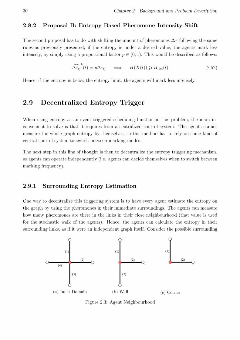
surrounding links, as if it were an independent graph itself. Consider the possible surrounding
(a) Inner Domain (b) Wall (c) Corner
Figure 2.3: Agent Neighbourhood
2.9. Decentralized Entropy Trigger 31
configurations for an agent in the graph presented in figure 2.3. Every link has a certain
pheromone value τi. Starting with the inner domain (a), and following the entropy expression
2.27 presented in Chapter 2, it is easy to calculate the entropy for the neighbour set of links Nas:
H(N ) =τ1
Tlog(
τ1
T) +
τ2
Tlog(
τ2
T) +
τ3
Tlog(
τ3
T) +
τ4
Tlog(
τ4
T) (2.53)
Where, same as in previous expressions, T is the sum of the pheromones in the considered links.
Now, lets evaluate this value in the minimum and maximum entropy situations. As defined
previously, the maximum entropy is found for an equal amount of pheromones in every link.
But we will consider the minimum entropy in this case to be that one where two of the links
have τi = 0 and the other two have the same amount. The reason for this is that this would be
the configuration to be expected in a graph that has converged to a unique solution; the ant
is always in a neighbourhood of two strongly marked links and two links marked with nearly
zero (see figure 3.1 for a converged graph). Hence, the minimum and maximum values are:
Hmax(N ) = log(4) = 2
Hmin(N ) = log(2) = 1
The lower limit in this case can be crossed; if an agent steps into a nearly-zero set of links,
the previous link to be walked will have a slightly higher value of pheromones, and that can
result in a value H ≤ 1. But it does represent the minimum to be expected in a graph that has
converged to only one solution. Now, considering the cases (b) and (c) in figure 2.3, one or two
links will be virtually added to the entropy calculation, and we will assign a value τ ∗ so that:
τ ∗ = max{τi}
That is, to compute the entropy in a case where the amount of surrounding links is less than
4, we will assign a value of pheromones to virtual links equal to the maximum value found
around the agent. This is done since entropy results depend on the size of the graph, and
taking max{τi} as the assigned value will yield a more conservative value of entropy. This will
cause an over-estimation of the entropy in certain cases, but it will also maintain the results
for a converged solution. This method will then be tested in Chapter 3.
32 Chapter 2. Background and Problem Description
2.10 Summary of Concepts
After introducing and expanding the background and necessary elements to understand and
analyze the problem, we present here the key points for the foundations of this work.
• First of all we presented the main structure of the algorithm to be studied, as well as the
background concepts of event-triggered control and stochastic theory necessary to fully
understand the analysis to be performed.
• In sections 2.4 and 2.5, the logic description of the algorithm and its expression as a
dynamic system was developed, to gain a better understanding of the behaviour of the
problem.
• To study this problem, the algorithm and its evolution, some metric concepts were pre-
sented. The most relevant one, given the structure of the problem, is the application
of Shannon Entropy (slightly modified from the original concept). This idea was fully
defined and explored, and how it relates to weighted graph we have in this particular
problem. Also, its relations with the convergence of the problem and its implications
were presented.
• Finally, the convergence of the graph to a certain solution was (partially) proven using
entropy as a random variable. Other metric parameters related to the convergence of the
graph and the efficiency of the solution generating behavior were presented and reasoned,
setting the base for the studies and analysis to be performed. And the proposals for event
triggered methods were presented, to be further analyzed in the experiments.
Chapter 3
Experimental Analysis and Results
In this chapter, more detailed information on the implementation of the algorithm is laid out,
as well as the simulation, performance and different case results for the algorithm.
The work will be focused on the following aspects:
• Describe the implementation of the algorithm, and present a baseline case to better
understand its behaviour, analyzing it in terms of the metrics presented previously.
• Study the convergence of the algorithm in terms of the entropy results.
• Suggest and study methods to implement an event-triggered routine into the algorithm.
• Study the impact this event-triggered method has on convergence and resource efficiency
(pheromones), and discuss its implementation.
3.1 Algorithm Implementation
According to the proprieties described previously, the algorithm runs as follows:
for time = 1, 2 ... end {for ant = 1, 2 ... N {
ant checks for surrounding pheromones
↓if ant has found goal ⇒ Xij = Xij
↓Compute new ant position following (2.8)
↓
33
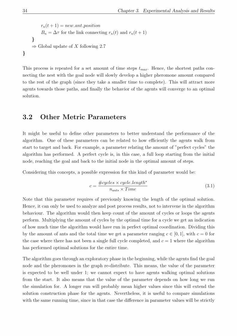
34 Chapter 3. Experimental Analysis and Results
rn(t+ 1) = new ant position
Bn = ∆τ for the link connecting rn(t) and rn(t+ 1)
}⇒ Global update of X following 2.7
}
This process is repeated for a set amount of time steps tmax. Hence, the shortest paths con-
necting the nest with the goal node will slowly develop a higher pheromone amount compared
to the rest of the graph (since they take a smaller time to complete). This will attract more
agents towards those paths, and finally the behavior of the agents will converge to an optimal
solution.
3.2 Other Metric Parameters
It might be useful to define other parameters to better understand the performance of the
algorithm. One of these parameters can be related to how efficiently the agents walk from
start to target and back. For example, a parameter relating the amount of ”perfect cycles” the
algorithm has performed. A perfect cycle is, in this case, a full loop starting from the initial
node, reaching the goal and back to the initial node in the optimal amount of steps.
Considering this concepts, a possible expression for this kind of parameter would be:
c =#cycles× cycle length∗
nants × Time(3.1)
Note that this parameter requires of previously knowing the length of the optimal solution.
Hence, it can only be used to analyze and post process results, not to intervene in the algorithm
behaviour. The algorithm would then keep count of the amount of cycles or loops the agents
perform. Multiplying the amount of cycles by the optimal time for a cycle we get an indication
of how much time the algorithm would have run in perfect optimal coordination. Dividing this
by the amount of ants and the total time we get a parameter ranging c ∈ [0, 1], with c = 0 for
the case where there has not been a single full cycle completed, and c = 1 where the algorithm
has performed optimal solutions for the entire time.
The algorithm goes through an exploratory phase in the beginning, while the agents find the goal
node and the pheromones in the graph re-distribute. This means, the value of the parameter
is expected to be well under 1; we cannot expect to have agents walking optimal solutions
from the start. It also means that the value of the parameter depends on how long we run
the simulation for. A longer run will probably mean higher values since this will extend the
solution construction phase for the agents. Nevertheless, it is useful to compare simulations
with the same running time, since in that case the difference in parameter values will be strictly
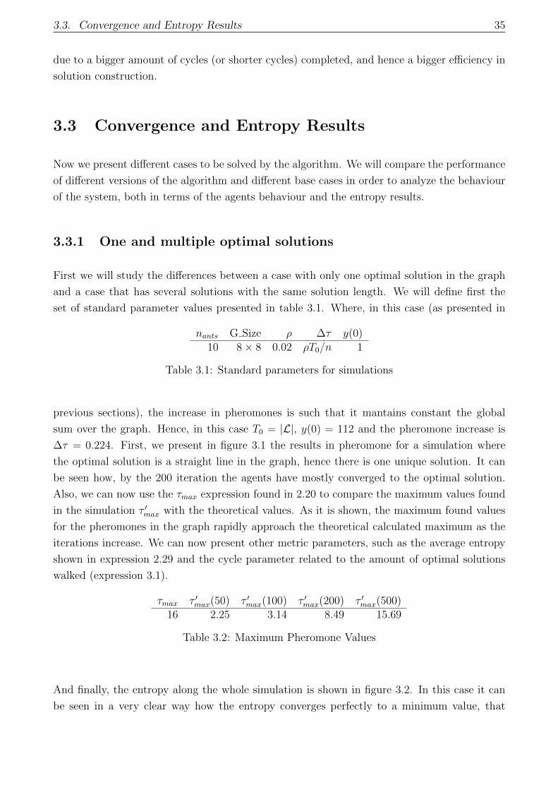
3.3. Convergence and Entropy Results 35
due to a bigger amount of cycles (or shorter cycles) completed, and hence a bigger efficiency in
solution construction.
3.3 Convergence and Entropy Results
Now we present different cases to be solved by the algorithm. We will compare the performance
of different versions of the algorithm and different base cases in order to analyze the behaviour
of the system, both in terms of the agents behaviour and the entropy results.
3.3.1 One and multiple optimal solutions
First we will study the differences between a case with only one optimal solution in the graph
and a case that has several solutions with the same solution length. We will define first the
set of standard parameter values presented in table 3.1. Where, in this case (as presented in
nants G Size ρ ∆τ y(0)10 8× 8 0.02 ρT0/n 1
Table 3.1: Standard parameters for simulations
previous sections), the increase in pheromones is such that it mantains constant the global
sum over the graph. Hence, in this case T0 = |L|, y(0) = 112 and the pheromone increase is
∆τ = 0.224. First, we present in figure 3.1 the results in pheromone for a simulation where
the optimal solution is a straight line in the graph, hence there is one unique solution. It can
be seen how, by the 200 iteration the agents have mostly converged to the optimal solution.
Also, we can now use the τmax expression found in 2.20 to compare the maximum values found
in the simulation τ ′max with the theoretical values. As it is shown, the maximum found values
for the pheromones in the graph rapidly approach the theoretical calculated maximum as the
iterations increase. We can now present other metric parameters, such as the average entropy
shown in expression 2.29 and the cycle parameter related to the amount of optimal solutions
walked (expression 3.1).
τmax τ ′max(50) τ ′max(100) τ ′max(200) τ ′max(500)16 2.25 3.14 8.49 15.69
Table 3.2: Maximum Pheromone Values
And finally, the entropy along the whole simulation is shown in figure 3.2. In this case it can
be seen in a very clear way how the entropy converges perfectly to a minimum value, that
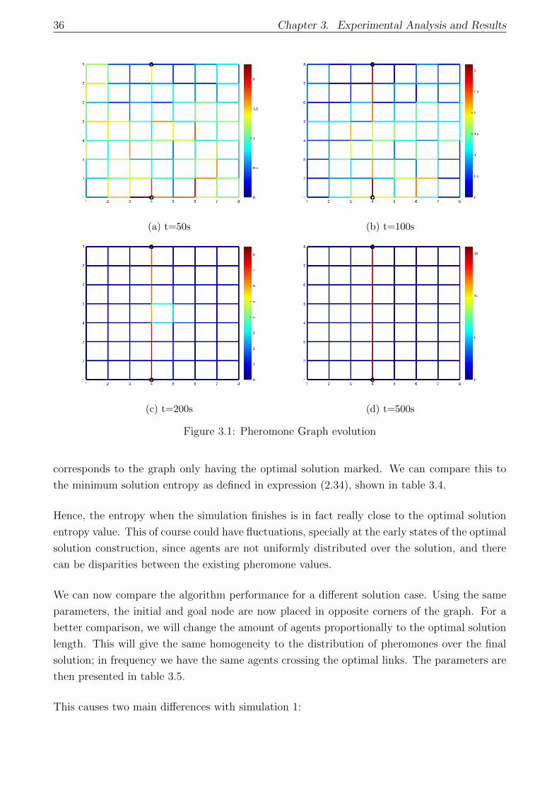
36 Chapter 3. Experimental Analysis and Results
(a) t=50s (b) t=100s
(c) t=200s (d) t=500s
Figure 3.1: Pheromone Graph evolution
corresponds to the graph only having the optimal solution marked. We can compare this to
the minimum solution entropy as defined in expression (2.34), shown in table 3.4.
Hence, the entropy when the simulation finishes is in fact really close to the optimal solution
entropy value. This of course could have fluctuations, specially at the early states of the optimal
solution construction, since agents are not uniformly distributed over the solution, and there
can be disparities between the existing pheromone values.
We can now compare the algorithm performance for a different solution case. Using the same
parameters, the initial and goal node are now placed in opposite corners of the graph. For a
better comparison, we will change the amount of agents proportionally to the optimal solution
length. This will give the same homogeneity to the distribution of pheromones over the final
solution; in frequency we have the same agents crossing the optimal links. The parameters are
then presented in table 3.5.
This causes two main differences with simulation 1:
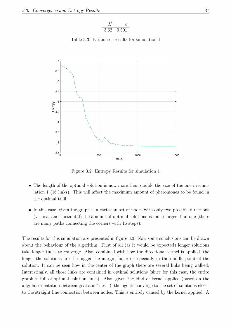
3.3. Convergence and Entropy Results 37
H c3.62 0.501
Table 3.3: Parameter results for simulation 1
Figure 3.2: Entropy Results for simulation 1
• The length of the optimal solution is now more than double the size of the one in simu-
lation 1 (16 links). This will affect the maximum amount of pheromones to be found in
the optimal trail.
• In this case, given the graph is a cartesian set of nodes with only two possible directions
(vertical and horizontal) the amount of optimal solutions is much larger than one (there
are many paths connecting the corners with 16 steps).
The results for this simulation are presented in figure 3.3. Now some conclusions can be drawn
about the behaviour of the algorithm. First of all (as it would be expected) longer solutions
take longer times to converge. Also, combined with how the directional kernel is applied, the
longer the solutions are the bigger the margin for error, specially in the middle point of the
solution. It can be seen how in the center of the graph there are several links being walked.
Interestingly, all those links are contained in optimal solutions (since for this case, the entire
graph is full of optimal solution links). Also, given the kind of kernel applied (based on the
angular orientation between goal and ”nest”), the agents converge to the set of solutions closer
to the straight line connection between nodes. This is entirely caused by the kernel applied. A
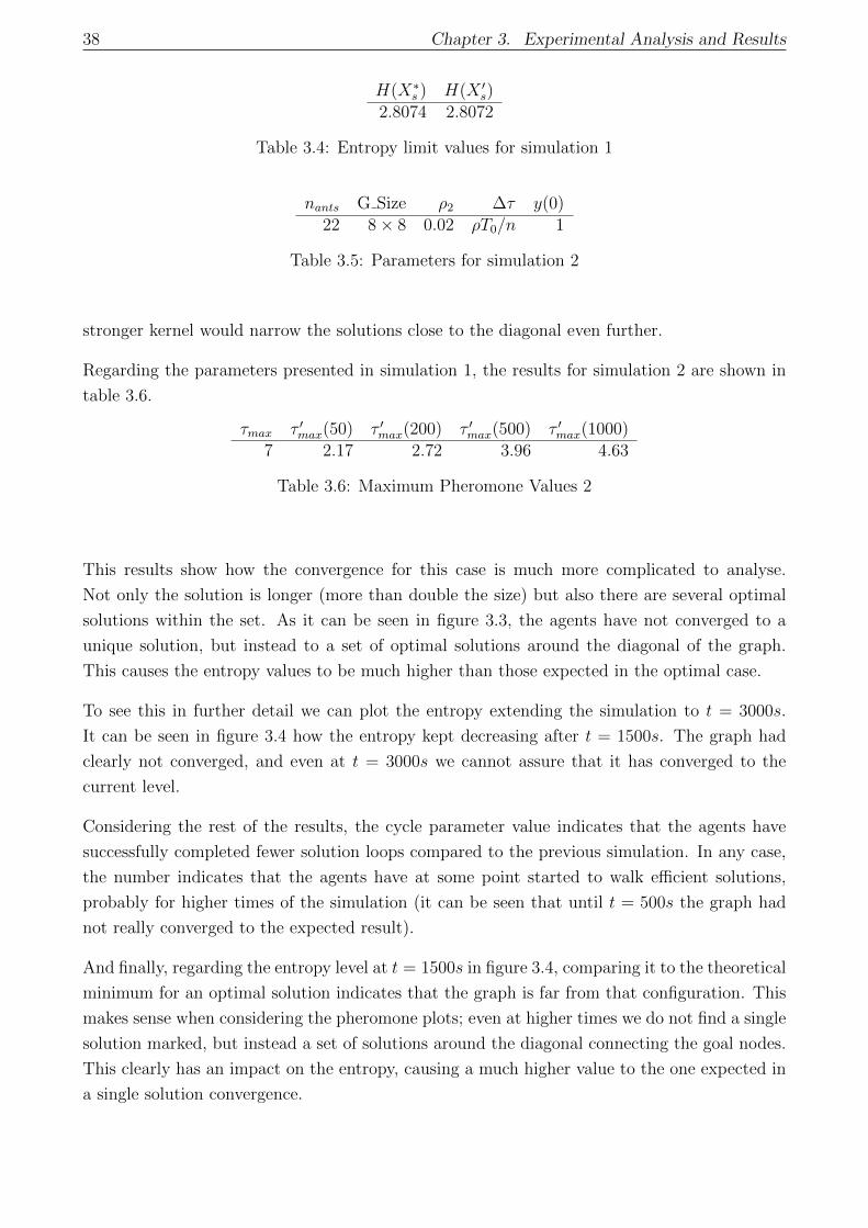
38 Chapter 3. Experimental Analysis and Results
H(X∗s ) H(X ′s)2.8074 2.8072
Table 3.4: Entropy limit values for simulation 1
nants G Size ρ2 ∆τ y(0)22 8× 8 0.02 ρT0/n 1
Table 3.5: Parameters for simulation 2
stronger kernel would narrow the solutions close to the diagonal even further.
Regarding the parameters presented in simulation 1, the results for simulation 2 are shown in
table 3.6.
τmax τ ′max(50) τ ′max(200) τ ′max(500) τ ′max(1000)7 2.17 2.72 3.96 4.63
Table 3.6: Maximum Pheromone Values 2
This results show how the convergence for this case is much more complicated to analyse.
Not only the solution is longer (more than double the size) but also there are several optimal
solutions within the set. As it can be seen in figure 3.3, the agents have not converged to a
unique solution, but instead to a set of optimal solutions around the diagonal of the graph.
This causes the entropy values to be much higher than those expected in the optimal case.
To see this in further detail we can plot the entropy extending the simulation to t = 3000s.
It can be seen in figure 3.4 how the entropy kept decreasing after t = 1500s. The graph had
clearly not converged, and even at t = 3000s we cannot assure that it has converged to the
current level.
Considering the rest of the results, the cycle parameter value indicates that the agents have
successfully completed fewer solution loops compared to the previous simulation. In any case,
the number indicates that the agents have at some point started to walk efficient solutions,
probably for higher times of the simulation (it can be seen that until t = 500s the graph had
not really converged to the expected result).
And finally, regarding the entropy level at t = 1500s in figure 3.4, comparing it to the theoretical
minimum for an optimal solution indicates that the graph is far from that configuration. This
makes sense when considering the pheromone plots; even at higher times we do not find a single
solution marked, but instead a set of solutions around the diagonal connecting the goal nodes.
This clearly has an impact on the entropy, causing a much higher value to the one expected in
a single solution convergence.
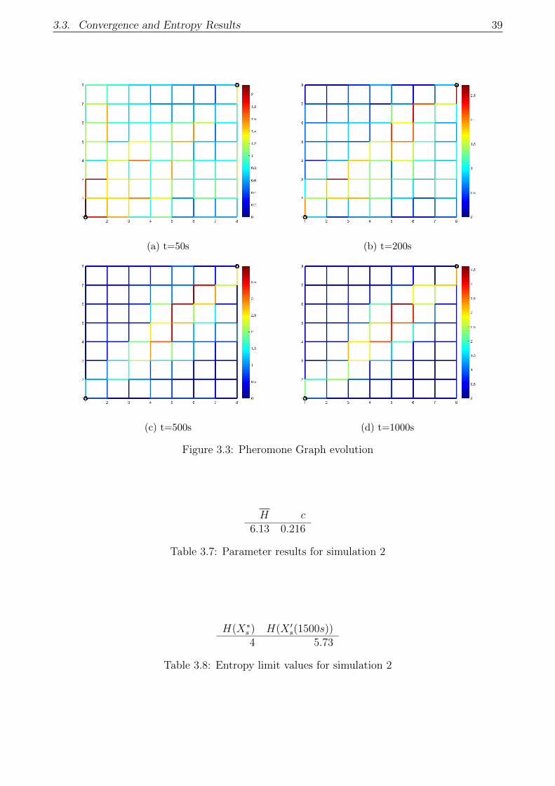
3.3. Convergence and Entropy Results 39
(a) t=50s (b) t=200s
(c) t=500s (d) t=1000s
Figure 3.3: Pheromone Graph evolution
H c6.13 0.216
Table 3.7: Parameter results for simulation 2
H(X∗s ) H(X ′s(1500s))4 5.73
Table 3.8: Entropy limit values for simulation 2
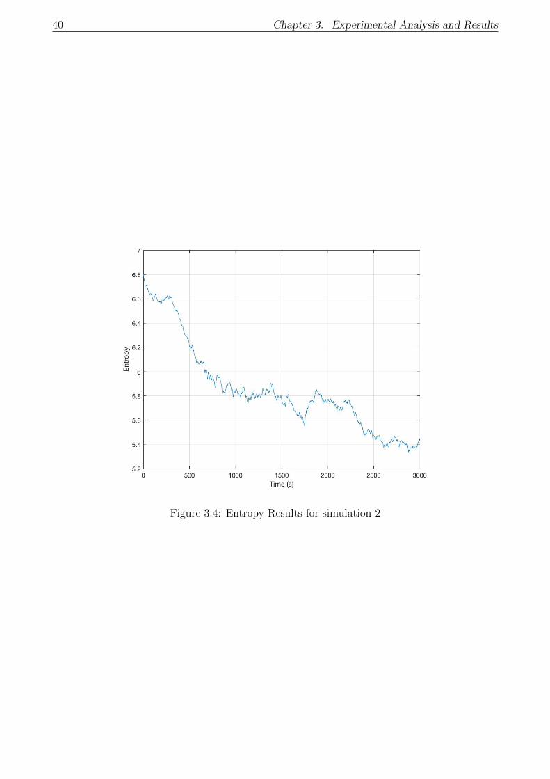
40 Chapter 3. Experimental Analysis and Results
Figure 3.4: Entropy Results for simulation 2

3.3. Convergence and Entropy Results 41
3.3.2 Parametric convergence analysis
We will now set up an experimental framework to study the influence of the parameters on the
convergence and behaviour of the algorithm. First, we will consider the algorithm characteristics
presented in table 3.9 to be fixed. The graph will then be similar to the one presented in figure
3.1. Then, the parameters to study are ρ and nants. We will do so by studying the impact
of both independently, running the algorithm 10 times for each combination of values and
averaging results. Also, to facilitate the task of comparing results, from now on the normalized
entropy described in 2.35 will be used as the standard metric, instead of the global entropy.
G Size |S∗| ∆τ y(0)8× 8 7 ρT0/n 1
Table 3.9: Parameters for Convergence Experiments
First, taking a standard value for nants = 15, the results of the study for the different values
of ρ are presented in table 3.10. The results are presented in terms of the average normalized
entropy (10 runs) of the simulation h, the normalized entropy after 500 time steps h(500), the
normalized entropy at the end (1500s) of the simulation hf , the cycle performance parameter c
and the convergence rate. The convergence rate is simply measuring which runs have converged
to an optimal solution following the convergence criteria presented in chapter 2.
ρ h h(500) hf c Converg. (%)0.005 0.556 0.678 0.229 0.365 200.01 0.354 0.409 0.044 0.411 1000.02 0.208 0.170 0.001 0.438 1000.03 0.171 0.136 0.016 0.442 900.04 0.161 0.108 0.016 0.440 800.05 0.134 0.048 0.016 0.445 900.06 0.178 0.099 0.092 0.403 300.07 0.206 0.122 0.128 0.386 300.08 0.359 0.318 0.281 0.228 300.09 0.280 0.228 0.216 0.275 200.10 0.245 0.199 0.192 0.291 30
Table 3.10: Experiment Results for nants = 15
A lot of interesting information can be extracted from this data. First, analyzing the conver-
gence values, it can be seen how for ρ ∈ [0.01, 0.05] the algorithm seems to converge with a
high probability. After this threshold, the convergence rates go down dramatically. Probably
because for higher evaporation rates agents can get trapped in unwanted regions of the graph,
hence increasing entropy rates and not achieving convergence. It also follows this logic that for
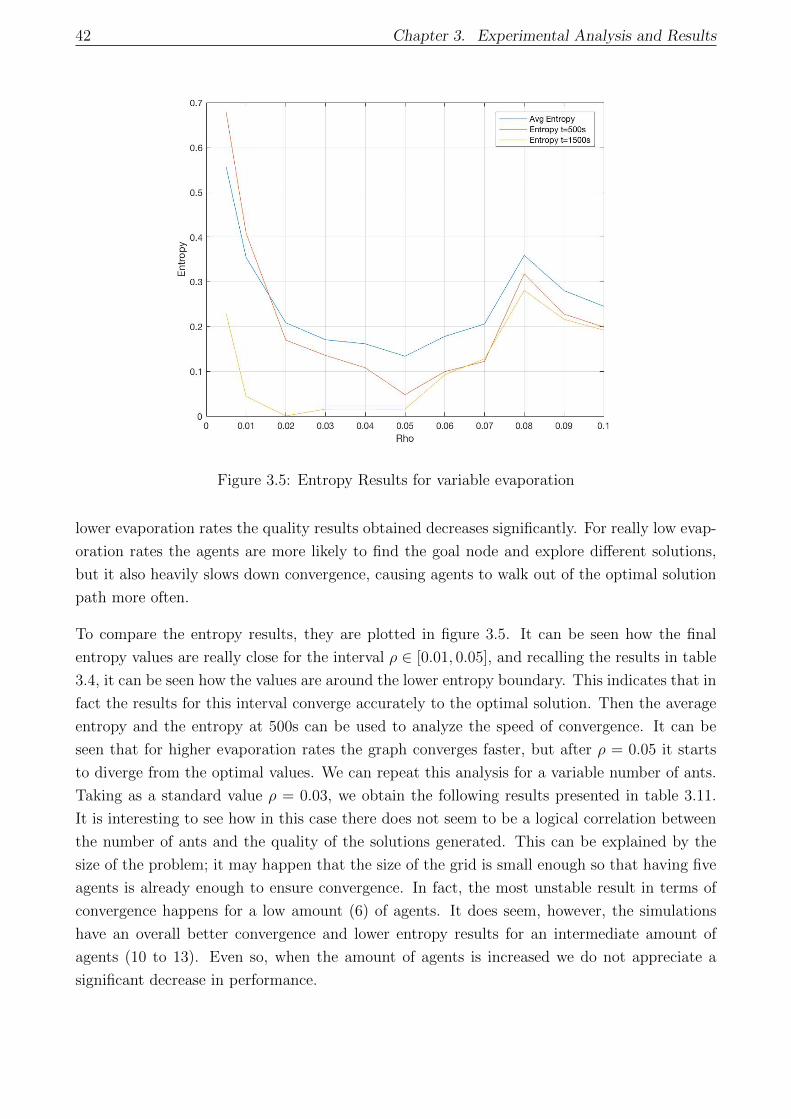
42 Chapter 3. Experimental Analysis and Results
Figure 3.5: Entropy Results for variable evaporation
lower evaporation rates the quality results obtained decreases significantly. For really low evap-
oration rates the agents are more likely to find the goal node and explore different solutions,
but it also heavily slows down convergence, causing agents to walk out of the optimal solution
path more often.
To compare the entropy results, they are plotted in figure 3.5. It can be seen how the final
entropy values are really close for the interval ρ ∈ [0.01, 0.05], and recalling the results in table
3.4, it can be seen how the values are around the lower entropy boundary. This indicates that in
fact the results for this interval converge accurately to the optimal solution. Then the average
entropy and the entropy at 500s can be used to analyze the speed of convergence. It can be
seen that for higher evaporation rates the graph converges faster, but after ρ = 0.05 it starts
to diverge from the optimal values. We can repeat this analysis for a variable number of ants.
Taking as a standard value ρ = 0.03, we obtain the following results presented in table 3.11.
It is interesting to see how in this case there does not seem to be a logical correlation between
the number of ants and the quality of the solutions generated. This can be explained by the
size of the problem; it may happen that the size of the grid is small enough so that having five
agents is already enough to ensure convergence. In fact, the most unstable result in terms of
convergence happens for a low amount (6) of agents. It does seem, however, the simulations
have an overall better convergence and lower entropy results for an intermediate amount of
agents (10 to 13). Even so, when the amount of agents is increased we do not appreciate a
significant decrease in performance.
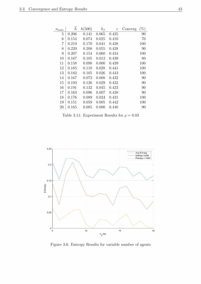
3.3. Convergence and Entropy Results 43
nants h h(500) hf c Converg. (%)5 0.206 0.141 0.065 0.435 906 0.154 0.074 0.025 0.410 707 0.219 0.170 0.041 0.438 1008 0.220 0.208 0.055 0.428 909 0.207 0.154 0.060 0.434 100
10 0.167 0.105 0.012 0.439 8011 0.158 0.098 0.000 0.439 10012 0.185 0.110 0.028 0.441 10013 0.182 0.105 0.026 0.443 10014 0.167 0.072 0.008 0.432 9015 0.193 0.126 0.029 0.432 9016 0.191 0.132 0.045 0.423 9017 0.163 0.096 0.007 0.438 9018 0.176 0.089 0.024 0.431 10019 0.151 0.059 0.005 0.442 10020 0.165 0.085 0.000 0.440 90
Table 3.11: Experiment Results for ρ = 0.03
Figure 3.6: Entropy Results for variable number of agents
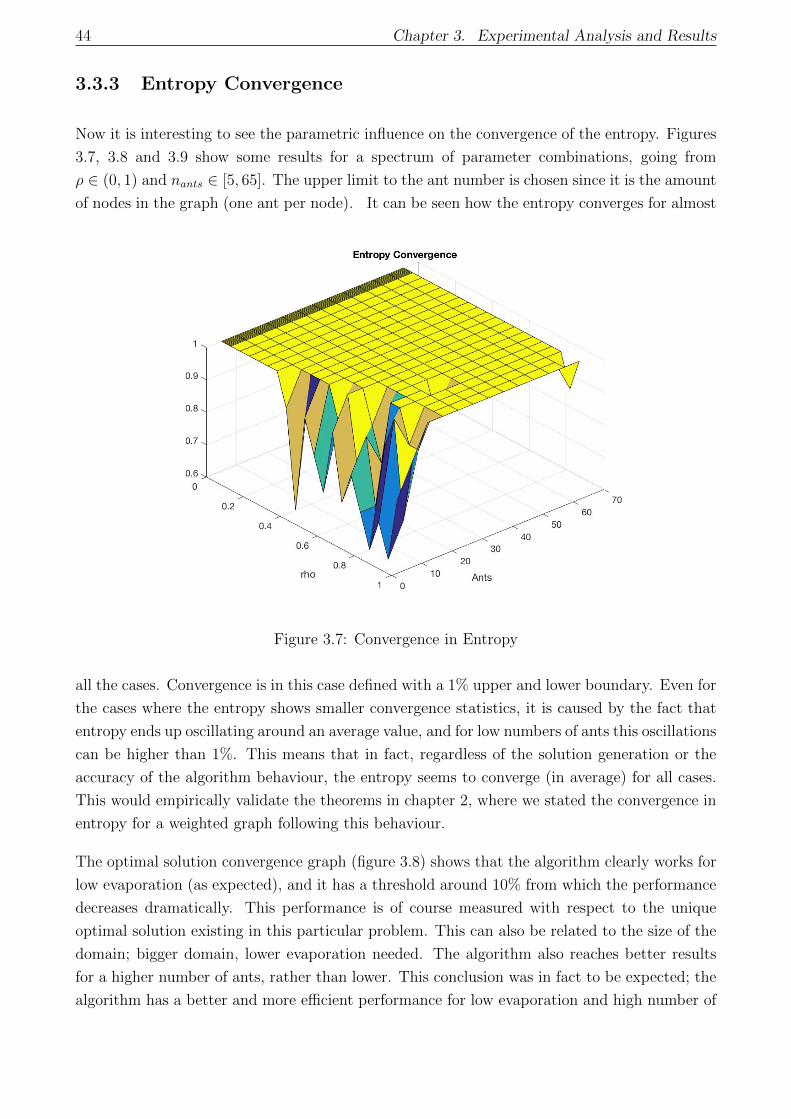
44 Chapter 3. Experimental Analysis and Results
3.3.3 Entropy Convergence
Now it is interesting to see the parametric influence on the convergence of the entropy. Figures
3.7, 3.8 and 3.9 show some results for a spectrum of parameter combinations, going from
ρ ∈ (0, 1) and nants ∈ [5, 65]. The upper limit to the ant number is chosen since it is the amount
of nodes in the graph (one ant per node). It can be seen how the entropy converges for almost
Figure 3.7: Convergence in Entropy
all the cases. Convergence is in this case defined with a 1% upper and lower boundary. Even for
the cases where the entropy shows smaller convergence statistics, it is caused by the fact that
entropy ends up oscillating around an average value, and for low numbers of ants this oscillations
can be higher than 1%. This means that in fact, regardless of the solution generation or the
accuracy of the algorithm behaviour, the entropy seems to converge (in average) for all cases.
This would empirically validate the theorems in chapter 2, where we stated the convergence in
entropy for a weighted graph following this behaviour.
The optimal solution convergence graph (figure 3.8) shows that the algorithm clearly works for
low evaporation (as expected), and it has a threshold around 10% from which the performance
decreases dramatically. This performance is of course measured with respect to the unique
optimal solution existing in this particular problem. This can also be related to the size of the
domain; bigger domain, lower evaporation needed. The algorithm also reaches better results
for a higher number of ants, rather than lower. This conclusion was in fact to be expected; the
algorithm has a better and more efficient performance for low evaporation and high number of
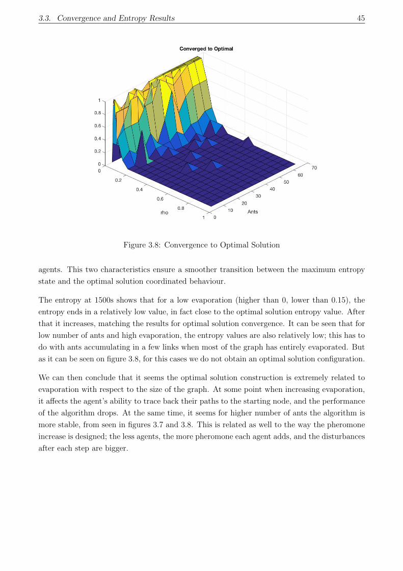
3.3. Convergence and Entropy Results 45
Figure 3.8: Convergence to Optimal Solution
agents. This two characteristics ensure a smoother transition between the maximum entropy
state and the optimal solution coordinated behaviour.
The entropy at 1500s shows that for a low evaporation (higher than 0, lower than 0.15), the
entropy ends in a relatively low value, in fact close to the optimal solution entropy value. After
that it increases, matching the results for optimal solution convergence. It can be seen that for
low number of ants and high evaporation, the entropy values are also relatively low; this has to
do with ants accumulating in a few links when most of the graph has entirely evaporated. But
as it can be seen on figure 3.8, for this cases we do not obtain an optimal solution configuration.
We can then conclude that it seems the optimal solution construction is extremely related to
evaporation with respect to the size of the graph. At some point when increasing evaporation,
it affects the agent’s ability to trace back their paths to the starting node, and the performance
of the algorithm drops. At the same time, it seems for higher number of ants the algorithm is
more stable, from seen in figures 3.7 and 3.8. This is related as well to the way the pheromone
increase is designed; the less agents, the more pheromone each agent adds, and the disturbances
after each step are bigger.
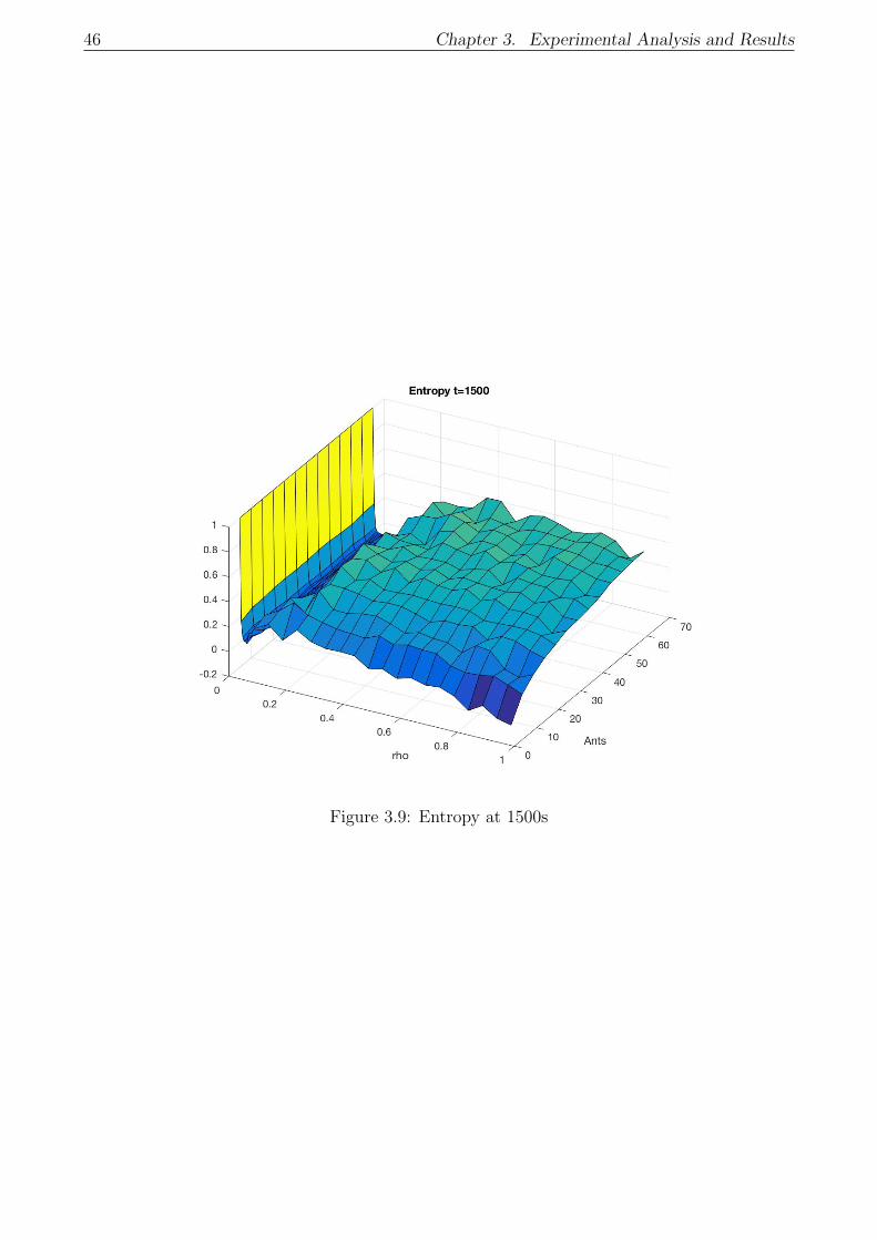
46 Chapter 3. Experimental Analysis and Results
Figure 3.9: Entropy at 1500s
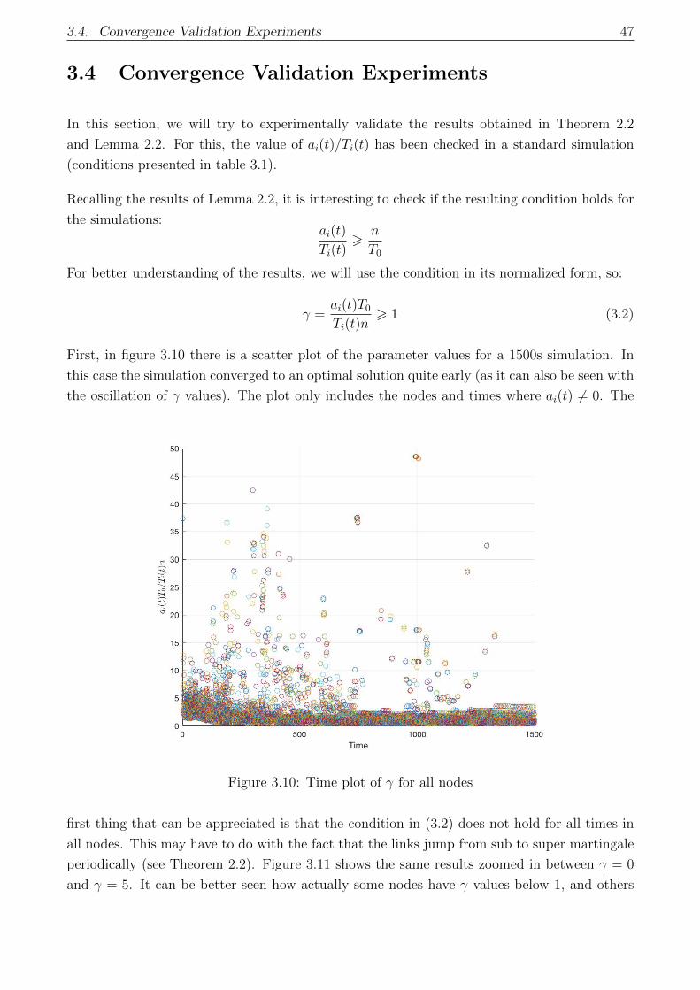
3.4. Convergence Validation Experiments 47
3.4 Convergence Validation Experiments
In this section, we will try to experimentally validate the results obtained in Theorem 2.2
and Lemma 2.2. For this, the value of ai(t)/Ti(t) has been checked in a standard simulation
(conditions presented in table 3.1).
Recalling the results of Lemma 2.2, it is interesting to check if the resulting condition holds for
the simulations:ai(t)
Ti(t)>
n
T0
For better understanding of the results, we will use the condition in its normalized form, so:
γ =ai(t)T0
Ti(t)n> 1 (3.2)
First, in figure 3.10 there is a scatter plot of the parameter values for a 1500s simulation. In
this case the simulation converged to an optimal solution quite early (as it can also be seen with
the oscillation of γ values). The plot only includes the nodes and times where ai(t) 6= 0. The
Figure 3.10: Time plot of γ for all nodes
first thing that can be appreciated is that the condition in (3.2) does not hold for all times in
all nodes. This may have to do with the fact that the links jump from sub to super martingale
periodically (see Theorem 2.2). Figure 3.11 shows the same results zoomed in between γ = 0
and γ = 5. It can be better seen how actually some nodes have γ values below 1, and others
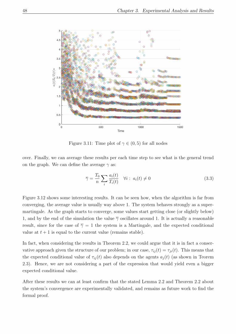
48 Chapter 3. Experimental Analysis and Results
Figure 3.11: Time plot of γ ∈ (0, 5) for all nodes
over. Finally, we can average these results per each time step to see what is the general trend
on the graph. We can define the average γ as:
γ =T0
n
∑i
ai(t)
Ti(t)∀i : ai(t) 6= 0 (3.3)
Figure 3.12 shows some interesting results. It can be seen how, when the algorithm is far from
converging, the average value is usually way above 1. The system behaves strongly as a super-
martingale. As the graph starts to converge, some values start getting close (or slightly below)
1, and by the end of the simulation the value γ oscillates around 1. It is actually a reasonable
result, since for the case of γ = 1 the system is a Martingale, and the expected conditional
value at t+ 1 is equal to the current value (remains stable).
In fact, when considering the results in Theorem 2.2, we could argue that it is in fact a conser-
vative approach given the structure of our problem; in our case, τij(t) = τji(t). This means that
the expected conditional value of τij(t) also depends on the agents aj(t) (as shown in Teorem
2.3). Hence, we are not considering a part of the expression that would yield even a bigger
expected conditional value.
After these results we can at least confirm that the stated Lemma 2.2 and Theorem 2.2 about
the system’s convergence are experimentally validated, and remains as future work to find the
formal proof.

3.4. Convergence Validation Experiments 49
Figure 3.12: Time plot of γ

50 Chapter 3. Experimental Analysis and Results
3.5 Entropy-Based Event Triggered Control
After the methods presented in Section 2.8, here we present the results of applying both pro-
posals.
3.5.1 Proposal A: Results
Now, using the same conditions as in 3.1, the algorithm variable values set for this method
simulations are presented in table 3.12.
nants G Size ρ1 ρ2 ∆τ y(0)10 8× 8 0.02 0.02 ρT0/n 1
Table 3.12: Parameters for Proposal A
In this case we can compute the entropy of the pheromone graph, and choose a simple entropy
boundary for the triggering condition. This is shown in figure 3.13. The dashed line represents
Figure 3.13: Entropy Computation and Entropy Limit Example
the entropy boundary; when the entropy goes above the line the algorithm will start to mark
with frequency 1, and with frequency f when it’s below. Considering these results, we can now
implement an event triggered control method for this case, choosing a value for f in expression
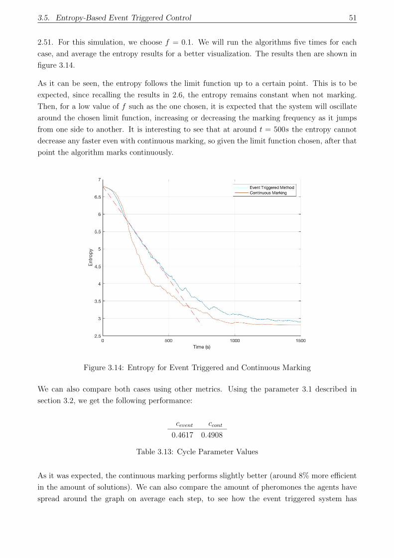
3.5. Entropy-Based Event Triggered Control 51
2.51. For this simulation, we choose f = 0.1. We will run the algorithms five times for each
case, and average the entropy results for a better visualization. The results then are shown in
figure 3.14.
As it can be seen, the entropy follows the limit function up to a certain point. This is to be
expected, since recalling the results in 2.6, the entropy remains constant when not marking.
Then, for a low value of f such as the one chosen, it is expected that the system will oscillate
around the chosen limit function, increasing or decreasing the marking frequency as it jumps
from one side to another. It is interesting to see that at around t = 500s the entropy cannot
decrease any faster even with continuous marking, so given the limit function chosen, after that
point the algorithm marks continuously.
Figure 3.14: Entropy for Event Triggered and Continuous Marking
We can also compare both cases using other metrics. Using the parameter 3.1 described in
section 3.2, we get the following performance:
cevent ccont
0.4617 0.4908
Table 3.13: Cycle Parameter Values
As it was expected, the continuous marking performs slightly better (around 8% more efficient
in the amount of solutions). We can also compare the amount of pheromones the agents have
spread around the graph on average each step, to see how the event triggered system has
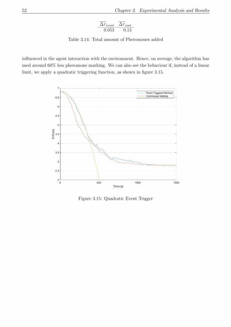
52 Chapter 3. Experimental Analysis and Results
∆τ event ∆τ cont0.053 0.13
Table 3.14: Total amount of Pheromones added
influenced in the agent interaction with the environment. Hence, on average, the algorithm has
used around 60% less pheromone marking. We can also see the behaviour if, instead of a linear
limit, we apply a quadratic triggering function, as shown in figure 3.15.
Figure 3.15: Quadratic Event Trigger
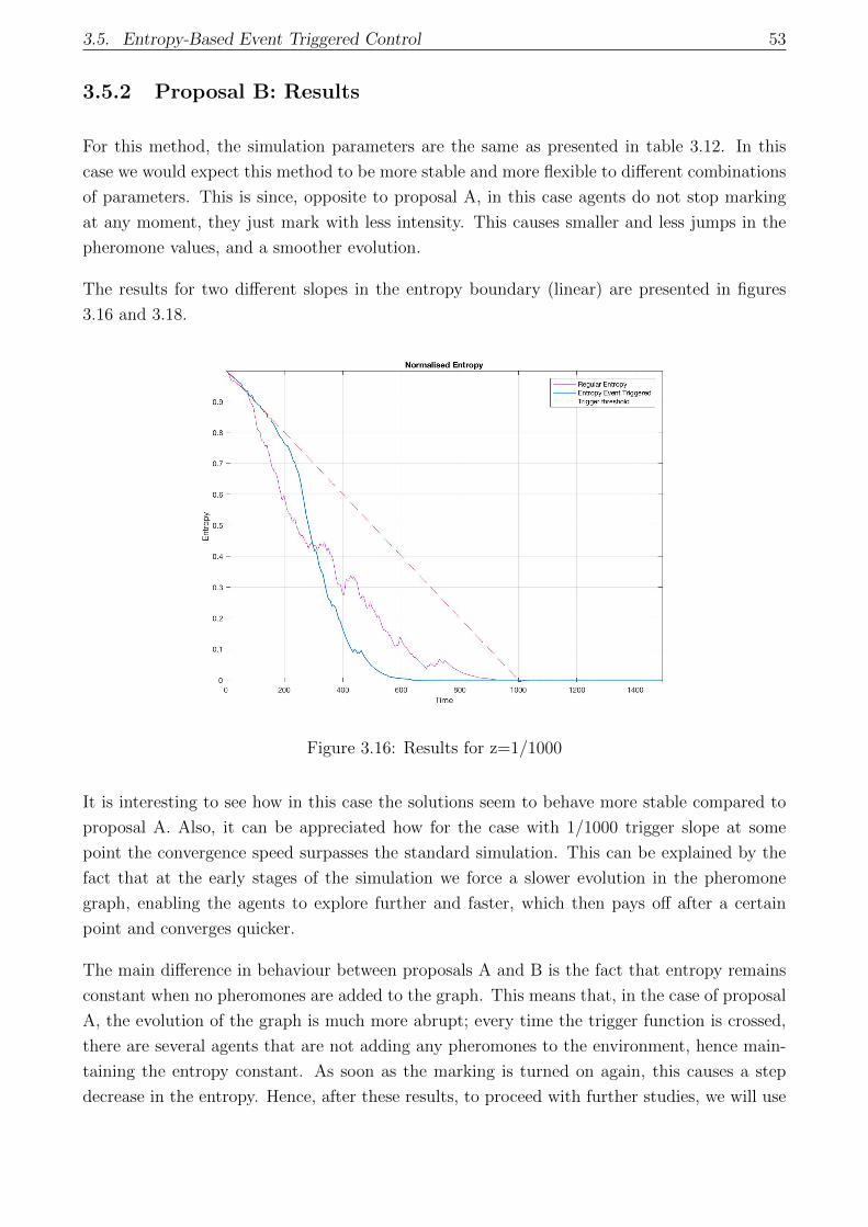
3.5. Entropy-Based Event Triggered Control 53
3.5.2 Proposal B: Results
For this method, the simulation parameters are the same as presented in table 3.12. In this
case we would expect this method to be more stable and more flexible to different combinations
of parameters. This is since, opposite to proposal A, in this case agents do not stop marking
at any moment, they just mark with less intensity. This causes smaller and less jumps in the
pheromone values, and a smoother evolution.
The results for two different slopes in the entropy boundary (linear) are presented in figures
3.16 and 3.18.
Figure 3.16: Results for z=1/1000
It is interesting to see how in this case the solutions seem to behave more stable compared to
proposal A. Also, it can be appreciated how for the case with 1/1000 trigger slope at some
point the convergence speed surpasses the standard simulation. This can be explained by the
fact that at the early stages of the simulation we force a slower evolution in the pheromone
graph, enabling the agents to explore further and faster, which then pays off after a certain
point and converges quicker.
The main difference in behaviour between proposals A and B is the fact that entropy remains
constant when no pheromones are added to the graph. This means that, in the case of proposal
A, the evolution of the graph is much more abrupt; every time the trigger function is crossed,
there are several agents that are not adding any pheromones to the environment, hence main-
taining the entropy constant. As soon as the marking is turned on again, this causes a step
decrease in the entropy. Hence, after these results, to proceed with further studies, we will use
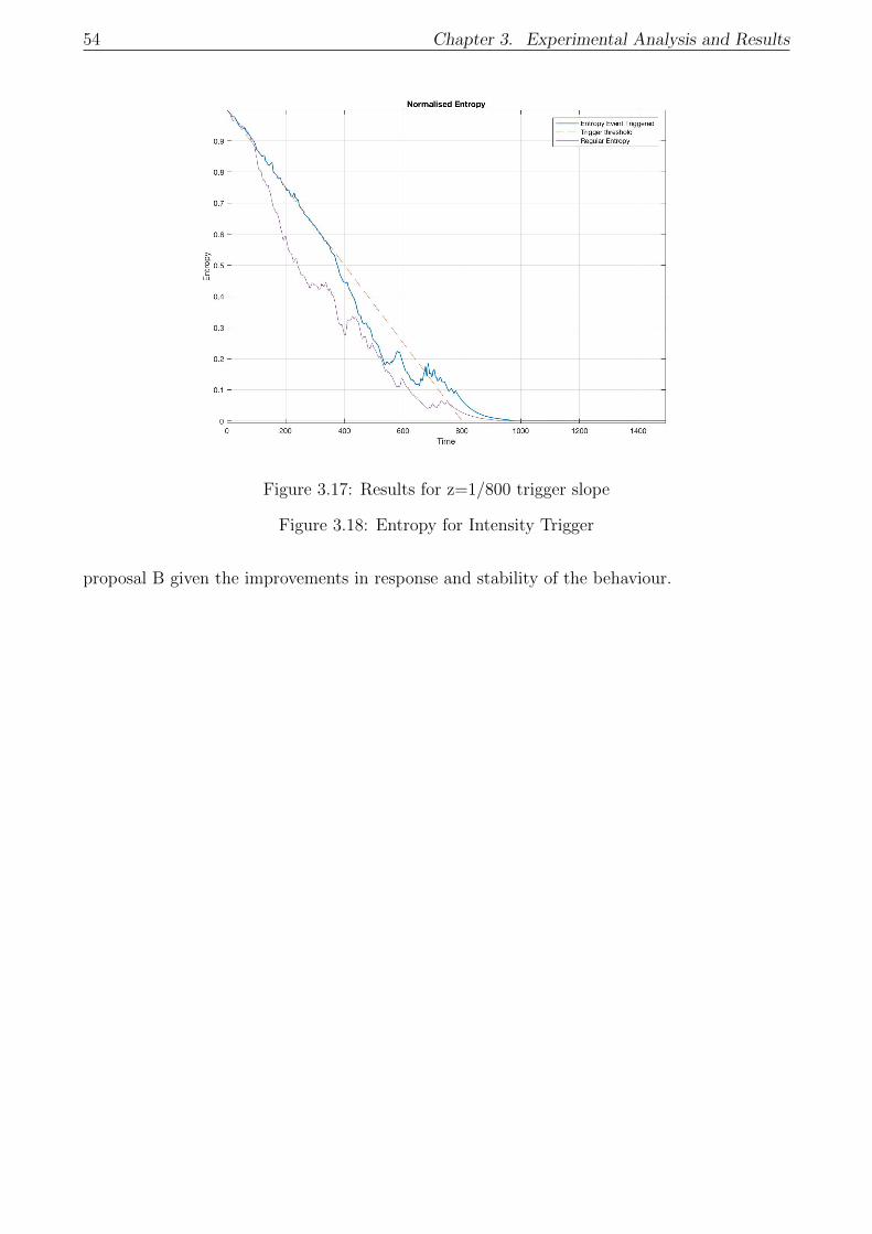
54 Chapter 3. Experimental Analysis and Results
Figure 3.17: Results for z=1/800 trigger slope
Figure 3.18: Entropy for Intensity Trigger
proposal B given the improvements in response and stability of the behaviour.

3.6. Decentralized Entropy Trigger: Results 55
3.6 Decentralized Entropy Trigger: Results
After the results in the previous section, proposal B is implemented with a decentralized scheme
based on the concepts in Section 2.9.
3.6.1 Entropy Estimation: Examples
In this case, we will apply the normalized entropy concept described in 2.35. The reason to
use a ratio as an indicator instead of the entropy value is because we want to estimate the
entire graph entropy using the local entropy value. Since the entropy will have a different value
just because both sets have a different size, it becomes useful to use a ratio in this case that
indicates how close the neighbourhood is to minimum entropy. Computing this parameter for
Figure 3.19: Global Entropy and Entropy Estimations
a simulation with the same conditions as presented in table 3.1, we get the results presented in
figure 3.19 for the global entropy and entropy estimation ratios for the agents.
It is interesting to see how the entropy estimation for the agents follows a similar trend to the
real entropy of the graph. Also, it can be seen how (as expected) at some point agents estimate
to have a lower entropy than the minimum entropy parameter. Nevertheless, it is useful to see
that agents can estimate the trend of the global entropy just by computing the entropy around
them. And most important, the agents estimation ratio goes to zero at the same time as the

56 Chapter 3. Experimental Analysis and Results
global entropy is converging. That makes sense since, when the agents are following a perfectly
marked path, the graph has converged and the entropy goes to the minimum value.
This becomes even clearer if we compute the average entropy estimated between all agents and
compare it to the normalized results for the global entropy. We define the average entropy as:
havg =
∑nantsi=1 hinants
(3.4)
With this, we can plot the average estimated entropy and the real measured entropy in the
graph.
Figure 3.20: Average Estimated Entropy and Real Time Entropy
As it can be seen in figure 3.20, the average of the estimated values is extremely similar to the
real computed entropy. This result was in fact to be expected; and the more agents we have,
the bigger area we use for estimating the entropy, and therefore the closer the values will get.
It can also be appreciated how the estimated entropy slightly underestimates the real entropy.
The reason for this can be that the agents tend to move in regions where there is lower local
entropy, and therefore strongly marked paths.
This method can in fact spark a more general discussion about complex interconnected systems,
and how their state can be estimated with a limited amount of observations scattered around
the system. In this case, sensing agents are able to estimate the level of chaos in the graph
by using their immediate neighbourhood. It is interesting to understand that in this case,
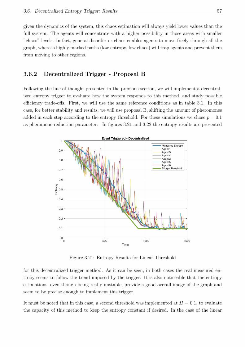
3.6. Decentralized Entropy Trigger: Results 57
given the dynamics of the system, this chaos estimation will always yield lower values than the
full system. The agents will concentrate with a higher possibility in those areas with smaller
”chaos” levels. In fact, general disorder or chaos enables agents to move freely through all the
graph, whereas highly marked paths (low entropy, low chaos) will trap agents and prevent them
from moving to other regions.
3.6.2 Decentralized Trigger - Proposal B
Following the line of thought presented in the previous section, we will implement a decentral-
ized entropy trigger to evaluate how the system responds to this method, and study possible
efficiency trade-offs. First, we will use the same reference conditions as in table 3.1. In this
case, for better stability and results, we will use proposal B, shifting the amount of pheromones
added in each step according to the entropy threshold. For these simulations we chose p = 0.1
as pheromone reduction parameter. In figures 3.21 and 3.22 the entropy results are presented
Figure 3.21: Entropy Results for Linear Threshold
for this decentralized trigger method. As it can be seen, in both cases the real measured en-
tropy seems to follow the trend imposed by the trigger. It is also noticeable that the entropy
estimations, even though being really unstable, provide a good overall image of the graph and
seem to be precise enough to implement this trigger.
It must be noted that in this case, a second threshold was implemented at H = 0.1, to evaluate
the capacity of this method to keep the entropy constant if desired. In the case of the linear
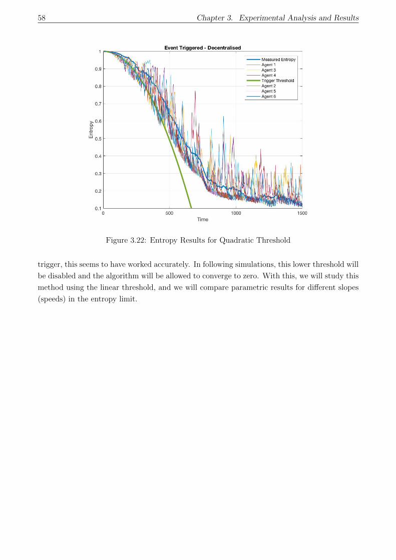
58 Chapter 3. Experimental Analysis and Results
Figure 3.22: Entropy Results for Quadratic Threshold
trigger, this seems to have worked accurately. In following simulations, this lower threshold will
be disabled and the algorithm will be allowed to converge to zero. With this, we will study this
method using the linear threshold, and we will compare parametric results for different slopes
(speeds) in the entropy limit.
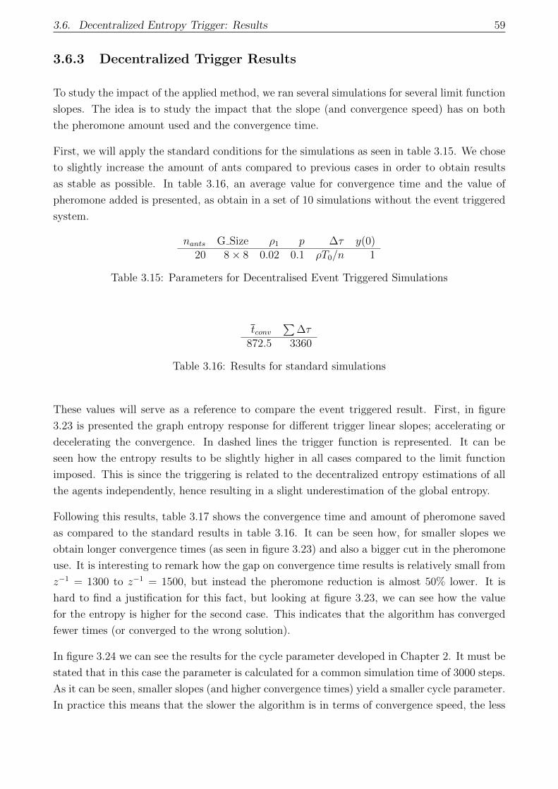
3.6. Decentralized Entropy Trigger: Results 59
3.6.3 Decentralized Trigger Results
To study the impact of the applied method, we ran several simulations for several limit function
slopes. The idea is to study the impact that the slope (and convergence speed) has on both
the pheromone amount used and the convergence time.
First, we will apply the standard conditions for the simulations as seen in table 3.15. We chose
to slightly increase the amount of ants compared to previous cases in order to obtain results
as stable as possible. In table 3.16, an average value for convergence time and the value of
pheromone added is presented, as obtain in a set of 10 simulations without the event triggered
system.
nants G Size ρ1 p ∆τ y(0)20 8× 8 0.02 0.1 ρT0/n 1
Table 3.15: Parameters for Decentralised Event Triggered Simulations
tconv∑
∆τ872.5 3360
Table 3.16: Results for standard simulations
These values will serve as a reference to compare the event triggered result. First, in figure
3.23 is presented the graph entropy response for different trigger linear slopes; accelerating or
decelerating the convergence. In dashed lines the trigger function is represented. It can be
seen how the entropy results to be slightly higher in all cases compared to the limit function
imposed. This is since the triggering is related to the decentralized entropy estimations of all
the agents independently, hence resulting in a slight underestimation of the global entropy.
Following this results, table 3.17 shows the convergence time and amount of pheromone saved
as compared to the standard results in table 3.16. It can be seen how, for smaller slopes we
obtain longer convergence times (as seen in figure 3.23) and also a bigger cut in the pheromone
use. It is interesting to remark how the gap on convergence time results is relatively small from
z−1 = 1300 to z−1 = 1500, but instead the pheromone reduction is almost 50% lower. It is
hard to find a justification for this fact, but looking at figure 3.23, we can see how the value
for the entropy is higher for the second case. This indicates that the algorithm has converged
fewer times (or converged to the wrong solution).
In figure 3.24 we can see the results for the cycle parameter developed in Chapter 2. It must be
stated that in this case the parameter is calculated for a common simulation time of 3000 steps.
As it can be seen, smaller slopes (and higher convergence times) yield a smaller cycle parameter.
In practice this means that the slower the algorithm is in terms of convergence speed, the less
60 Chapter 3. Experimental Analysis and Results
Figure 3.23: Entropy Results for several slopes
z−1 tconv τsaved(%)600 1045 5.48700 1209 6.52800 1208 10.27900 1397 10.29
1050 1503 13.461200 1598 18.851300 1801 21.061500 1820 31.08
Table 3.17: Results for different slopes
amount of full cycles will be able to complete. This result is logical; a slower convergence means
a more spread out pheromone graph, and hence a more chaotic agent behaviour. Finally, figure
3.25 shows a plot of the convergence time versus the amount of pheromones saved, with a
linear interpolation to illustrate the general trend. These results show that it is then possible
to establish a trade-off between pheromone usage and convergence time, and this trade-off
seems to have an almost linear behaviour for the studied range of parameters. It also shows
how the use of estimated entropy instead of real computed entropy affects the response on the
graph; there is an under estimation of the entropy, hence obtaining measured results that are
slightly over the designed trigger threshold. Nevertheless, the threshold seems to impose an
overall behaviour trend, slowing down the convergence and increasing the efficiency overall.
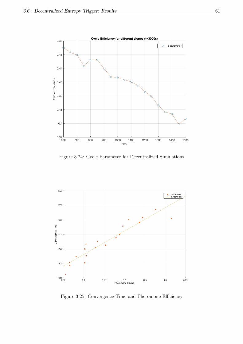
3.6. Decentralized Entropy Trigger: Results 61
Figure 3.24: Cycle Parameter for Decentralized Simulations
Figure 3.25: Convergence Time and Pheromone Efficiency
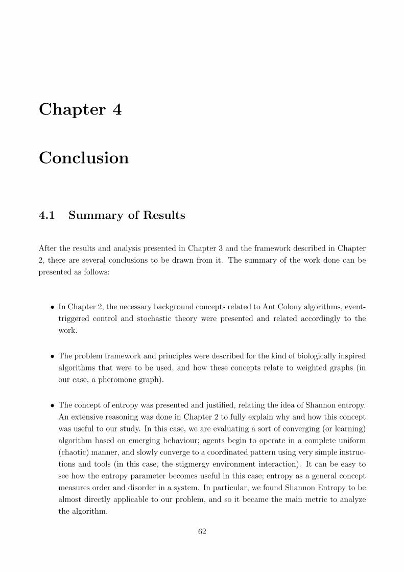
Chapter 4
Conclusion
4.1 Summary of Results
After the results and analysis presented in Chapter 3 and the framework described in Chapter
2, there are several conclusions to be drawn from it. The summary of the work done can be
presented as follows:
• In Chapter 2, the necessary background concepts related to Ant Colony algorithms, event-
triggered control and stochastic theory were presented and related accordingly to the
work.
• The problem framework and principles were described for the kind of biologically inspired
algorithms that were to be used, and how these concepts relate to weighted graphs (in
our case, a pheromone graph).
• The concept of entropy was presented and justified, relating the idea of Shannon entropy.
An extensive reasoning was done in Chapter 2 to fully explain why and how this concept
was useful to our study. In this case, we are evaluating a sort of converging (or learning)
algorithm based on emerging behaviour; agents begin to operate in a complete uniform
(chaotic) manner, and slowly converge to a coordinated pattern using very simple instruc-
tions and tools (in this case, the stigmergy environment interaction). It can be easy to
see how the entropy parameter becomes useful in this case; entropy as a general concept
measures order and disorder in a system. In particular, we found Shannon Entropy to be
almost directly applicable to our problem, and so it became the main metric to analyze
the algorithm.
62
4.1. Summary of Results 63
• Reasoned analysis was presented in Chapter 2 to justify the convergence and stability
of these kind of algorithms. Even though we did not get solid proof of this convergence
(Conjecture 2.1) for our particular case, given the results in Theorem 2.2 and Lemma
2.2 (as well as the experimental results in section 3.4) we remain confident that our
modifications to the algorithm did not alter the main properties of convergence presented
for other Ant Colony algorithms.
• After having the background and secondary concepts properly laid out, in Chapter 3 we
presented the particular description and implementation of our algorithm, and a set of
test results to further understand how the algorithm behaves. And also to demonstrate
how the concept of entropy was in this case describing the coordination and convergence of
the system, and how different configurations and solutions have an impact on the metrics
used.
• Considering these foundations, we proceeded to implement an event-triggered scheme to
the algorithm. Two methods were tested, both using entropy as a defining function for
the state of the system: First a triggered switch between marking frequencies, and second
a triggered switch between marking intensities. The second option was found to be the
most stable and the one that yields better results. This is to be expected when considering
the global evolution of the algorithm and the fact that, in general, smoothness in graph
evolution leads to better solutions.
• Finally, this method was implemented and analyzed using the metric parameters pre-
sented in previous chapters, and one important modification was introduced. In event-
triggered control it is interesting to decentralize the scheduling of control tasks. In our
particular case this means letting each agent ”decide” when to trigger the control task
without having to rely on a centralized state computation (entropy) and a centralized
command. It can be seen how in the case of autonomous agents, decentralized schemes
become even more interesting. For this, the concept of estimated local entropy was in-
troduced, letting each agent extrapolate the global entropy in the graph using only its
neighbourhood links. This turned out to yield better results than expected, and the
amount of resources saved was finally presented, relating it to convergence time. As ex-
pected in a system of these characteristics, a longer convergence time leads to a bigger
saving in resource usage.
64 Chapter 4. Conclusion
4.2 Applications
There are different levels on the possible applications of this work, from the metric parame-
ters developed to the understanding of the algorithm itself. These can be summarized in the
following points:
• First, the idea of using entropy (in this case Shannon Entropy) to analyze learning or
emerging behaviour algorithms. This becomes really useful when evaluating autonomous
agent systems that evolve from a chaotic state to a coordinated and structured pattern.
Some particular criteria must be met in order to apply this concept, but we believe it
could be applied to other autonomous agent applications, and could provide interesting
insight on the characteristics of the systems.
• Another application, further down the line, would be to use these modified Ant Colony
algorithms as control schemes for large autonomous agent systems. Work has already
been done in this direction (see [6], [7]), and it would be interesting to extend it to more
complex behaviour and more complex systems (swarms of drones being a natural step).
• In this same line of thought, our results implementing decentralized event-triggered
schemes could also have applications for swarm robotics systems. As it was seen on the
results presented in Chapter 3, our proposal directly relates convergence time to resource
optimization. When implementing these algorithms in larger swarms of smaller agents,
resource optimization will become a key performance aspect (in this case, resource opti-
mization can refer to amount of data exchanged, network load, battery usage, autonomy
loss...).
• Finally, on a more conceptual approach, this work could have direct applications for co-
ordination of automated transport systems, for example. It could be the foundation for a
traffic coordination system in cities, calculating and modifying routes but also controlling
each vehicle independently as an agent.
4.3. Future Work 65
4.3 Future Work
There are some important aspects that could be subject of further and deeper work. First, it
would be important to develop a solid formal proof verifying the convergence of these algorithms.
As mentioned before, there is proof that certain kind of Ant Colony algorithms converge, and
that they converge to an optimal solution, but it would be interesting to try to find a similar
proof for our modified version. The reasoning presented in Chapter 2 is just an indication on
the likelihood of convergence, and cannot be considered a solid proof.
Then, following the previous conclusions on possible applications, it would be interesting to start
implementing this version on autonomous agent physical systems, specially when incorporating
the event triggered schemes, and see how they impact the behaviour of a robotic swarm. This
would be the first step to tackle further applications in this area. This line of work was initially
planned for this Master Thesis, but given the limited available time it was not possible to start
working in this area.
Finally, considering the algorithm study it could be useful to start applying modifications
to the algorithm, with a final implementation in mind, and study the changes in efficiency
and response. For example, experimenting with a variable ∆τ and letting agents interact more
heavily with the graph, cancelling or modifying links at once, could lead to better performances.
Also the exploration of other biologically inspired algorithms and the application of the metrics
developed here could lead to a better control scheme, that could incorporate characteristics of
different algorithms in a sort of efficient hybrid scheme.
Bibliography
[1] Dorigo M. Optimization, learning and natural algorithms. PhD Thesis, Politecnico di
Milano, Italy, 1991.
[2] Dorigo M, Maniezzo V, and Colorni A. Ant system: Optimization by a colony of cooper-
ating agents. IEEE Trans Syst Man Cybernet Part B, 26(1):29–41, 1996.
[3] Traniello J F A. Foraging strategies of ants. Ann. Rev. Entomol., 34:191–210, 1989.
[4] Blum C. Ant colony optimization: Introduction and recent trends. Physics of Life Reviews,
2(4):353–373, 2005.
[5] Marco Dorigo and Luca Maria Gambardella. Ant colony system: a cooperative learning
approach to the traveling salesman problem. IEEE Transactions on evolutionary compu-
tation, 1(1):53–66, 1997.
[6] Alers S, Tuyls K, Ranjbar-Sahraei B, Claes D, and Weiss G. Insect-inspired robot coordi-
nation: Foraging and coverage. Artificial Life, 14:761–768, 2014.
[7] Alers S, Claes D, Tuyls K, and Weiss G. Biologically inspired multi-robot foraging. In
Proceedings of the 2014 international conference on Autonomous agents and multi-agent
systems, pages 1683–1684. International Foundation for Autonomous Agents and Multia-
gent Systems, 2014.
[8] Sjriek Alers, Daan Bloembergen, Daniel Hennes, Steven De Jong, Michael Kaisers, Nyree
Lemmens, Karl Tuyls, and Gerhard Weiss. Bee-inspired foraging in an embodied swarm. In
The 10th International Conference on Autonomous Agents and Multiagent Systems-Volume
3, pages 1311–1312. International Foundation for Autonomous Agents and Multiagent
Systems, 2011.
[9] Paulo Tabuada. Event-triggered real-time scheduling of stabilizing control tasks. IEEE
Transactions on Automatic Control, 52(9):1680–1685, 2007.
[10] Robert G Gallager. Discrete Stochastic Processes. Springer Science + Business Media,
New York, 1996.
[11] J. Jacod and P. Protter. Probability Essentials. Springer, Berlin, 2000.
66

BIBLIOGRAPHY 67
[12] Robert M Gray. Entropy and information theory. Springer Science & Business Media,
2011.
[13] Shannon C.E. A mathematical theory of communication. The Bell System Technical
Journal, 27:379–423, 1948.
[14] Timo Mulder and Jorn Peters. Entropy rate of stochastic processes. 2015.
[15] Walter J Gutjahr. A graph-based ant system and its convergence. Future generation
computer systems, 16(8):873–888, 2000.
[16] Walter J Gutjahr. Aco algorithms with guaranteed convergence to the optimal solution.
Information processing letters, 82(3):145–153, 2002.
[17] Thomas Stutzle and Marco Dorigo. A short convergence proof for a class of ant colony
optimization algorithms. IEEE Transactions on evolutionary computation, 6(4):358–365,
2002.


TRITA TRITA-MAT-E 2017:74
ISRN -KTH/MAT/E--17/74--SE
www.kth.se