ansys thermal assignment

University of Victoria MECH420 – Finite Element Methods Summer 2012

By: Majid Soleimaninia

Tutorial for Assignment #3 Heat Transfer Analysis

By ANSYS (Mechanical APDL) V.13.0

1 Problem Description This exercise consists of an analysis of an electronics component cooling design using fins: All

electronic components generate heat during the course of their operation. To ensure optimal

working of the component, the generated heat needs to be removed. This is done by attaching

fins to the device which aid in rapid heat removal to the surroundings. For the sake of simplicity,

we’ll assume that the electronic circuit is made of copper with thermal conductivity of 386

W/mºK and that it generates heat at the rate of 1 W. The enclosing container is made of a steel

with thermal conductivity of 17 W/mºK. The fins are made of aluminum with thermal

conductivity of 180 W/mºK. There is convection along all the boundaries except the bottom,

which is insulated. The film (convection) coefficient is h=50 W/m2ºK and the ambient

temperature is 20ºC.

Figure 1: Problem geometry

1.1 OBJECTIVE: Determine an optimal number of fins to use on the component. Cases considered should all use

an odd number of fins (3, 5, 7, …).



1.2 Deliverables: A hardcopy submission that includes:

1. A plot of the temperature distribution in the component for the baseline case of 3 cooling

fins and for your recommended number of fins.

2. A plot generated using Matlab that shows the reduction of the maximum temperature in

the component as a function of the number of fins.

Students are encouraged to collaborate with each other by distributing the tasks of modeling the

specific cases (each case differing in only the number of fins used). Submissions must be

prepared individually.

2 Start ANSYS (Mechanical APDL) V.13.0 Begin ANSYS (Mechanical APDL) with Start → All Programs → ANSYS 13.0 →

Mechanical APDL (ANSYS). That will bring you to the main ANSYS Utility Menu as seen in

Figure 2 .

Figure 2: Opening ANSYS to the Utility Menu and graphics window.



3 Preprocessing: Defining the Problem

3.1 Select job name and analysis type

The various menus below will sometimes get moved to a back (hidden) window. If you think

that has occurred hit the Raise Hidden button, . You will always need a job name:

1. Utility Menu → File → Change Jobname.

2. Change_Jobname, type in the new name, OK (as seen in Figure 3).

The ANSYS file sizes for real engineering problems get to be quite large, so have a directory

dedicated to ANSYS:

1. Utility Menu → File → Change Directory.

2. Browse for Folder → Change Working Directory, pick your directory (ANSYS

Tutorial_P5-70 in Figure 4), OK.

Figure 3: Setting the new job name.



To keep up with your analysis studies over time create descriptive titles:

1. Utility Menu → File → Change Title.

2. Change Title, enter a descriptive title, OK (see Figure 5).

Figure 4: Establish a directory for the analysis files.

Figure 5: Provide a descriptive title.



3.2 Element type data As in the conduction example, we will use PLANE55 (Thermal Solid, Quad 4node 55). This

element can be used as a plane element or as an axisymmetric ring element with a 2-D thermal

conduction capability. The element has four nodes with a single degree of freedom, temperature,

at each node. The element is applicable to a 2-D, steady-state or transient thermal analysis. The

element can also compensate for mass transport heat flow from a constant velocity field.

1. Main Menu → Preferences → Preferences for GUI Filtering.

2. Check Thermal, accept default h-Method, OK, as in Figure 6. (This is a thermal

Problem)

3. Main Menu → Preprocessor → Element Type → Add/Edit/Delete, as in Figure 7.

4. In Element Types, seen in Figure 7, pick Add → Library of Element Types.

5. Select (Thermal Mass) Solid and Quad 4 node 55 (that is, PLANE55), OK.

6. In Element Types window, select PLANE55 element and then pick Options… to

modify your PLANE55 element type options, as in Figure 8.

7. In Element Types pick Close.

Figure 6: Declare the selection of a thermal analysis.



3.3 Define member material properties Here you will use the simplest thermal, isotropic, 1D material description. ANSYS has full

anisotropic (completely directionally dependent), as well as non-linear material “constitutive

laws”. We need to define three different materials (Copper, Aluminum and Steel). At first we are

defining Copper then Aluminum and at the end, Steel. Activate the material properties with:

Figure 7: Select Thermal Solid, Quad 4node 55 (PLANE55) element type.

Figure 8: Modify PLANE55 element type options.



1. Main Menu → Preprocessor → Material Props → Material Models.

2. Material Model Number 1 appears in Define Material Model Behavior.

3. Double click on Thermal, then Conductivity, then Isotropic.

4. In Conductivity for Material Number 1 enter 0.386 (W/mmoK) for thermal conductivity,

KXX, for Copper, as in Figure 9, OK.

5. Close (X) the Define Material Model Behavior window.

Activate the material properties for Aluminum with:


2. Click Material → New Models… in Define Material Model Behavior.

3. In Define Material ID enter 2 for new material, Aluminum, OK, as in Figure 10

4. Material Model Number 2 appears in Define Material Model Behavior, Select it.

5. Click on Thermal, then Conductivity, then Isotropic.


KXX, for Aluminum, as in Figure 11, OK.


Figure 9: Define material properties for Copper.



To activate the material properties for Steel, again:


2. Click Material → New Models… in Define Material Model Behavior.

3. In Define Material ID enter 3 for new material, Steel, OK, as in Figure 10

4. Material Model Number 3 appears in Define Material Model Behavior, Select it.

5. Click on Thermal, then Conductivity, then Isotropic.


KXX, for Steel, as in Figure 11, OK.


Figure 10: Define the new material model in list.

Figure 11: Define material properties for Aluminum.



3.4 Create Geometry Of course, ANSYS has powerful mesh generation capabilities. However, for beginners or small

problems with only a few nodes you can type in the coordinates, or make your domain by areas,

or use cursor input via the graphics window, or read them from a file. Use the second approach:

1. Main Menu → Preprocessor → Modeling → Create → Areas → Rectangle → By 2

Corners.

2. In Rectangle by 2 Corners of Figure 14 enter coordinates of your main big rectangular

area (A1), WP X = 0, WP Y = 0, Width = 50, Height = 50 (mm), OK.

3. If you make a mistake you can return and correct it with Main Menu → Preprocessor

→ Modeling →Move/Modify → Areas →Areas, or delete it with Main Menu →

Preprocessor → Modeling →Delete →Areas Only.

Figure 12: Define the new material model in list.

Figure 13: Define material properties for Steel.



Now, plot the geometry by area number:

1. Utility Menu → PlotCtrls → Numbering.

2. In Plot Numbering Controls check Area numbers, OK.

3. Utility Menu → PlotCtrls → Numbers and review the plot that is similar to Figure 14.

4. To get the reverse video white background of that figure use PlotCtrls → Style → Color

→ Reverse Video.

To make two other small rectangular areas in top of our domain which we should subtract them

from the main domain, you can do the same procedure;


Corners.

2. In Rectangle by 2 Corners of Figure 15 enter coordinates of small rectangular area (A2),

WP X = 10, WP Y = 40, Width = 10, Height = 10 (mm), OK.

Figure 14: Build the main area



Also for the other one;


Corners.

2. In Rectangle by 2 Corners of Figure 16 enter coordinates of small rectangular area (A3),

WP X = 30, WP Y = 40, Width = 10, Height = 10 (mm), OK.

Figure 15: Build the small areas.



Now you can subtract the small rectangular areas (A2 & A3) from the main big rectangular areas

(A1):

1. Main Menu → Preprocessor → Modeling → Operate → Booleans → Subtract →

Area.

2. In Subtract Areas of Figure 17 select the main area (A1) by clicking on it. Note: The

selected area will turn pink once it is selected. Click 'OK' on the 'Subtract Areas'

window. Now you should select the areas to be subtracted, select the smaller rectangles

(A2 &A3) by clicking on them and then click 'OK'. Now, your model should be like

Figure 17 and have the new rectangular area (A4) as you see.

Figure 16: Build the small areas.



To make the Copper section (Heat Generator) and we could:

1. Main Menu → Preprocessor → Modeling → Create → Keypoints → In Active CS

2. In Create Keypoints in Active Coordinate System of Figure 18, enter number and

coordinates of Copper rectangular section keypoints,

i. NPT= 100, X = 20, Y = 10, Z = 0, Apply.

ii. NPT= 200, X = 30, Y = 10, Z = 0, Apply.

iii. NPT= 300, X = 30, Y = 20, Z = 0, Apply.

iv. NPT= 400, X = 20, Y = 20, Z = 0, Apply.

Figure 17: Building geometry.



3. Main Menu → Preprocessor → Modeling → Create → Lines → In Active Coord

4. Now in Lines in Active Coord of Figure 19, create lines by picking the exciting

keypoints:

i. Picking the Keypoints Number= 100 (a square symbol appears), then pick

Keypoints Number= 200.

ii. Picking the Keypoints Number= 200 (a square symbol appears), then pick


iii. Picking the Keypoints Number= 300 (a square symbol appears), then pick


iv. Picking the Keypoints Number= 400 (a square symbol appears), then pick


Figure 18: Defining the Keypoints to build Copper rectangular section.



5. Main Menu → Preprocessor → Modeling → Operate → Booleans → Divide → Area

by Line.

6. In Divide Areas by Line of Figure 20 select the main area (A4) by clicking on it. Note:

The selected area will turn pink once it is selected. Click 'OK' on the 'Subtract Areas'

window. Now you should select the lines to be divided, select the lines which we just

made by keyponits by clicking on them and then click 'OK'. Now, your model should be

like Figure 21 and have two new areas (A1&A2) as you see.

Figure 19: Defining the Lines to build Copper rectangular section .



Figure 20: Dividing the main Area to two areas.

Figure 21: Divided Areas ( A1 & A2) .



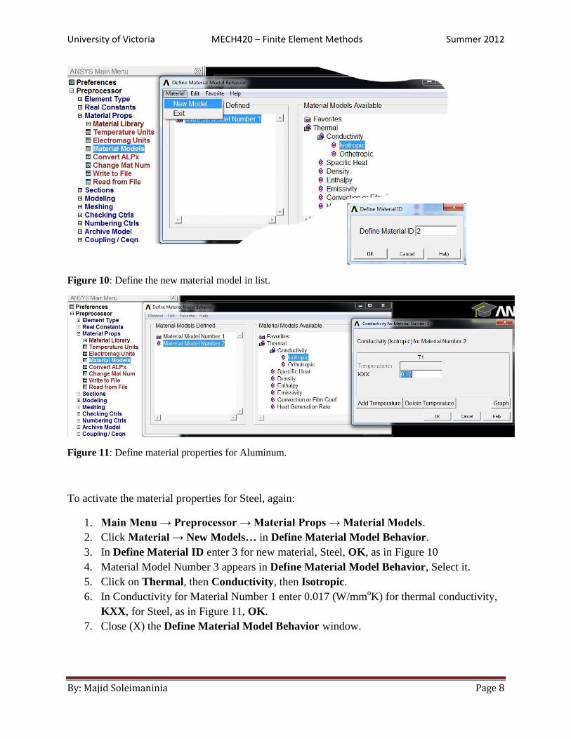
To make the Aluminum section (Fins) and we could:

7. Main Menu → Preprocessor → Modeling → Create → Keypoints → In Active CS

8. In Create Keypoints in Active Coordinate System of Figure 22, enter number and

coordinates of Aluminum section keypoints,

v. NPT= 500, X = 0, Y = 30, Z = 0, Apply.

vi. NPT= 600, X = 50, Y = 30, Z = 0, Apply.

9. Main Menu → Preprocessor → Modeling → Create → Lines → In Active Coord

10. Now in Lines in Active Coord of Figure 23, create lines by picking the exciting

keypoints:

v. Picking the Keypoints Number= 500 (a square symbol appears), then pick


Figure 22: Defining the Keypoints to build Aluminum section.



11. Main Menu → Preprocessor → Modeling → Operate → Booleans → Divide → Area

by Line.

12. In Divide Areas by Line select the main area (A2) by clicking on it. Note: The selected

area will turn pink once it is selected. Click 'OK' on the 'Subtract Areas' window. Now

you should select the lines to be divided, select the lines which we just made by

keyponits by clicking on them and then click 'OK'. Now, the final model should be like

Figure 24 and have three new areas (A1, A3 & A4) as you see.

Figure 23: Defining the Lines to build Aluminum section.



You also can see the list of all areas to distinguish them easily, Figure 25. Here the A1 is the

Copper section, A3 is the Aluminum section and the A4 is the Steel section.

Figure 24: Divided Areas (A1, A3 & A4).

Figure 25: List of Areas.



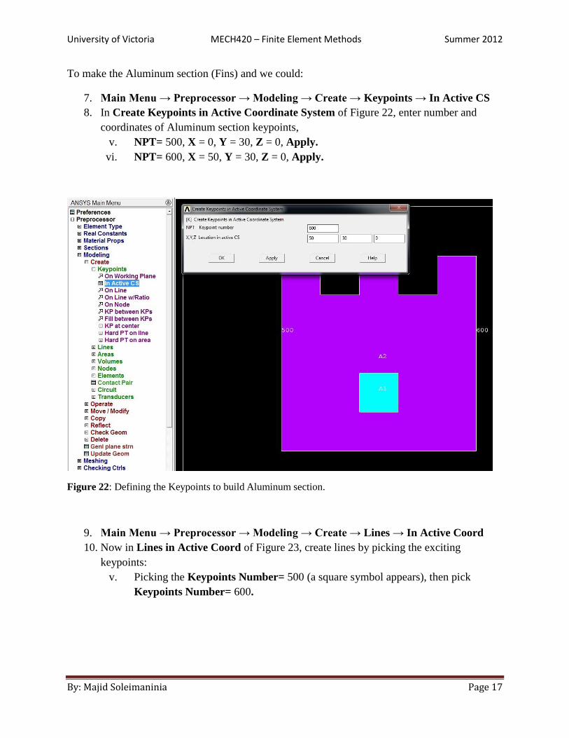
3.5 Define material & element attributes Next you have to associate each of the areas with your previous material numbers and element.

1. Main Menu → Preprocessor → Meshing → Mesh Attribute → Picked Areas.

2. In Area Attributes, seen in Figure 26, pick the small rectangle Copper area (A1). Note:

there will be a Multiple-Entities window appears to select the correct area, OK.

3. In Area Attributes, seen in Figure 27, select (Material number = 1, Real constant set

= None, Element type number = 1 PLANE55, Element coordinate sys = 0, Element

section = None), OK.

Define the Material attribute for other areas (A3 & A4) in the same way, just change Material

number =2 for A3 and Material number =3 for A4.

Figure 26: Define material & element attributes.



3.6 Mesh Size 1. Main Menu → Preprocessor → Meshing → Size Cntrls → Areas → All Areas.

2. In Element Size on All Selected Area, seen in Figure 28, enter Size Element edge

length = 1, OK.

Figure 27: Define material 1 to picked Area (A1).

Figure 28: Define mesh size.



3.7 Meshing 1. Main Menu → Preprocessor → Meshing → Mesh → Areas → Free.

2. In Mesh Areas, seen in Figure 29, click on Pick All, OK.

3.8 Define Analysis Type

1. Main Menu → Preprocessor → Loads → Analysis Type → New Analysis.

2. In New Analysis, seen in Figure 29, pick Steady-State, OK.

Figure 29: Meshing the geometry.

Figure 30: Define Analysis type.



3.9 Apply Constraints In this problem all sides of block have convection type of boundary condition except the bottom

side which is isolated.

In order to apply convection Boundary Conditions:

1. Main Menu → Preprocessor → Loads → Define Loads→ Apply → Thermal→

Convection → On lines.

2. In Apply CONV on Lines, seen in Figure 31, select all the lines which are on the left,

right and top sides except the bottom line, OK.

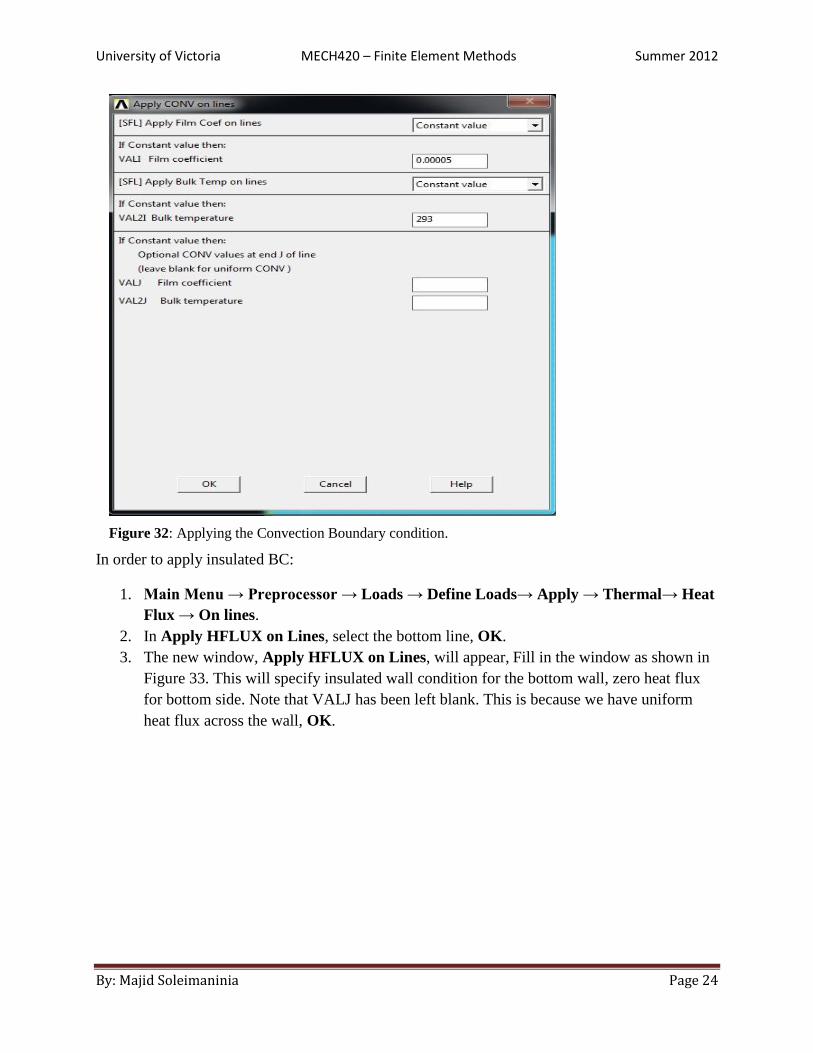
3. The new window, Apply CONV on Lines, will appear, Fill in the window as shown in

Figure 32. This will specify a convection of 0.00005 W/mm2.K and an ambient

temperature of 293 Kelvin. Note that VALJ and VAL2J have been left blank. This is

because we have uniform convection across the line, OK.

Figure 31: Define the Boundary conditions to apply Convection.



In order to apply insulated BC:

1. Main Menu → Preprocessor → Loads → Define Loads→ Apply → Thermal→ Heat

Flux → On lines.

2. In Apply HFLUX on Lines, select the bottom line, OK.

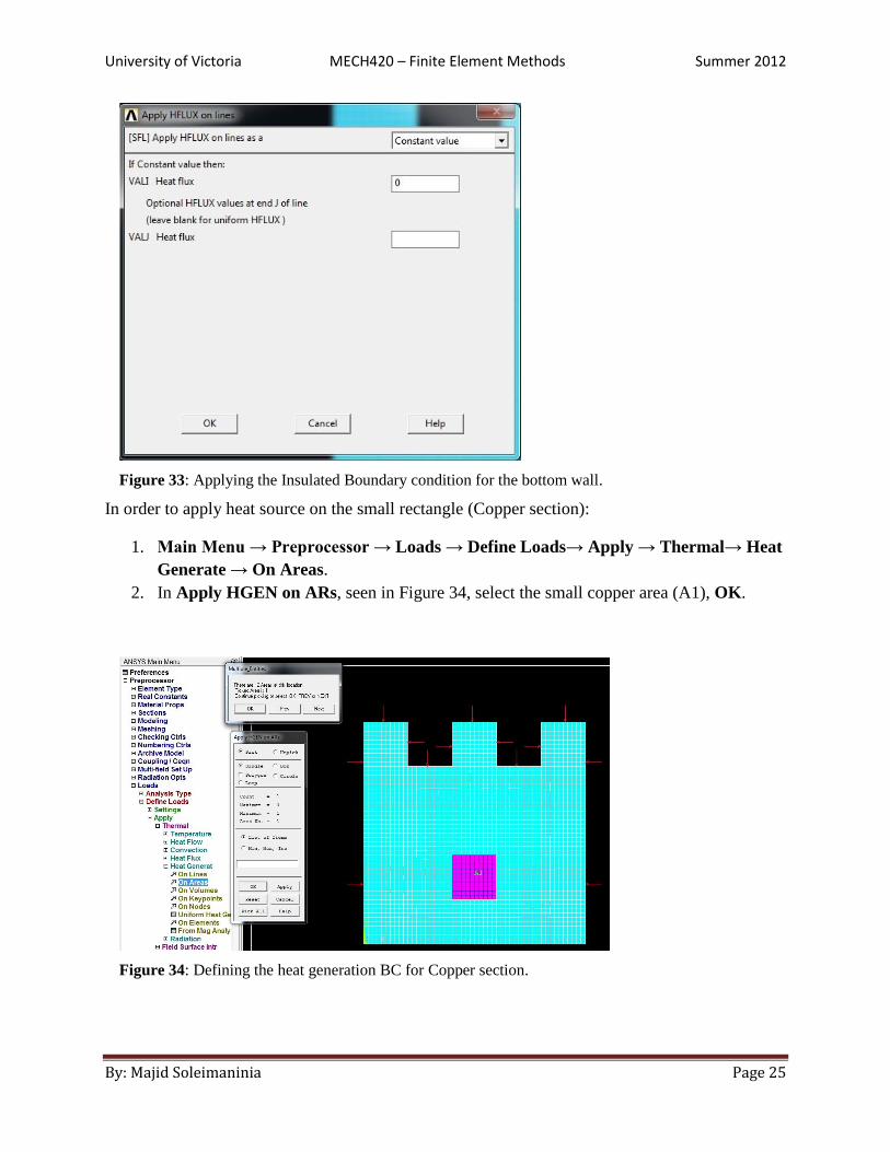
3. The new window, Apply HFLUX on Lines, will appear, Fill in the window as shown in

Figure 33. This will specify insulated wall condition for the bottom wall, zero heat flux

for bottom side. Note that VALJ has been left blank. This is because we have uniform

heat flux across the wall, OK.

Figure 32: Applying the Convection Boundary condition.



In order to apply heat source on the small rectangle (Copper section):

1. Main Menu → Preprocessor → Loads → Define Loads→ Apply → Thermal→ Heat

Generate → On Areas.

2. In Apply HGEN on ARs, seen in Figure 34, select the small copper area (A1), OK.

Figure 33: Applying the Insulated Boundary condition for the bottom wall.

Figure 34: Defining the heat generation BC for Copper section.



3. The new window, Apply HGEN on areas, will appear, Fill in the window as shown in

Figure 35. This will specify 0.01 W/mm2 heat generation rate on area section, OK.

4 Solve the model To use the current (and only) load system (LS) enter:

1. Main Menu → Solution → Solve → Current LS, review the listed summary, OK.

2. When the solution of the simultaneous equations is complete you will be alerted that the

solution is done.

Figure 35: Applying the heat source on Copper section.



Figure 36: Solving for the current load set.

5 Post-processing

5.1 Plot Temperature

It is always wise to visually check the computed displacements:

1. Main Menu → General Postproc → Plot Results → Contour Plot→ Nodal Solu.

2. In Contour Nodal Solution Data, seen in Figure 37, → DOF Solution→ Nodal

Temperature, OK.

Figure 37: plotting the nodal temperature results.



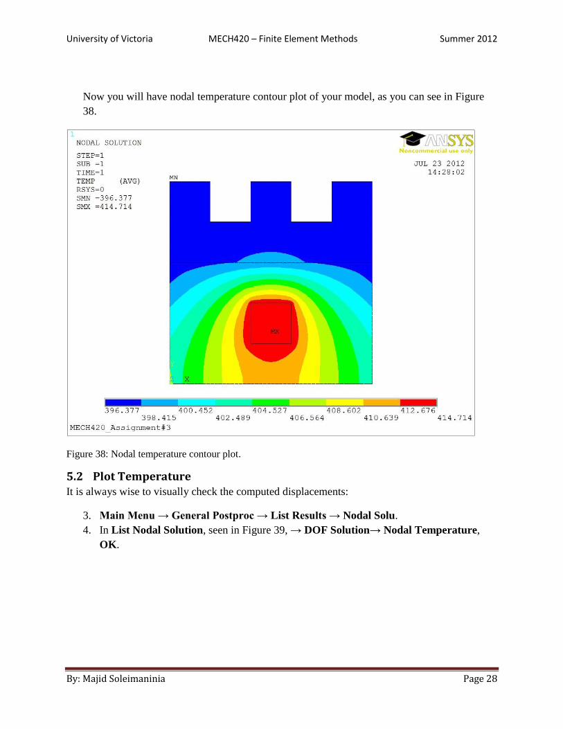
Now you will have nodal temperature contour plot of your model, as you can see in Figure

38.

Figure 38: Nodal temperature contour plot.

5.2 Plot Temperature It is always wise to visually check the computed displacements:

3. Main Menu → General Postproc → List Results → Nodal Solu.

4. In List Nodal Solution, seen in Figure 39, → DOF Solution→ Nodal Temperature,

OK.



Figure 39: Listing Nodal temperature result.

ansys thermal assignment

Documents

Transcript of ansys thermal assignment