Meshing of a detailed DrivAer Body with ANSYS Meshing and ...
Upload
etienne-rochaCategory
view
1.811download
104
8/10/2019 ANSYS Meshing Users Guide
http://slidepdf.com/reader/full/ansys-meshing-users-guide 1/491
ANSYS Meshing User's Guide
Release 15.0ANSYS, Inc.November 2013Southpointe
275 Technology DriveCanonsburg, PA 15317 ANSYS, Inc. is
certified to ISO9001:2008.
http://www.ansys.com(T ) 724-746-3304
(F) 724-514-9494

8/10/2019 ANSYS Meshing Users Guide
http://slidepdf.com/reader/full/ansys-meshing-users-guide 2/491
Copyright and Trademark Information
© 2013 SAS IP, Inc. All rights reserved. Unauthorized use, distribution or duplication is prohibited.
ANSYS, ANSYS Workbench, Ansoft, AUTODYN, EKM, Engineering Knowledge Manager, CFX, FLUENT, HFSS and any
and all ANSYS, Inc. brand, product, service and feature names, logos and slogans are registered trademarks ortrademarks of ANSYS, Inc. or its subsidiaries in the United States or other countries. ICEM CFD is a trademark used
by ANSYS, Inc. under license. CFX is a trademark of Sony Corporation in Japan. All other brand, product, serviceand feature names or trademarks are the property of their respective owners.
Disclaimer Notice
THIS ANSYS SOFTWARE PRODUCT AND PROGRAM DOCUMENTATION INCLUDE TRADE SECRETS AND ARE CONFID-ENTIAL AND PROPRIETARY PRODUCTS OF ANSYS, INC., ITS SUBSIDIARIES, OR LICENSORS. The software productsand documentation are furnished by ANSYS, Inc., its subsidiaries, or affiliates under a software license agreement
that contains provisions concerning non-disclosure, copying, length and nature of use, compliance with exportinglaws, warranties, disclaimers, limitations of liability, and remedies, and other provisions. The software products
and documentation may be used, disclosed, transferred, or copied only in accordance with the terms and conditionsof that software license agreement.
ANSYS, Inc. is certified to ISO 9001:2008.
U.S. Government Rights
For U.S. Government users, except as specifically granted by the ANSYS, Inc. software license agreement, the use,duplication, or disclosure by the United States Government is subject to restrictions stated in the ANSYS, Inc.
software license agreement and FAR 12.212 (for non-DOD licenses).
Third-Party Software
See the legal information in the product help files for the complete Legal Notice for ANSYS proprietary software
and third-party software. If you are unable to access the Legal Notice, please contact ANSYS, Inc.
Published in the U.S.A.
8/10/2019 ANSYS Meshing Users Guide
http://slidepdf.com/reader/full/ansys-meshing-users-guide 3/491
Table of Contents
Capabilities in ANSYS Workbench . . . . . . . . . . . . . . . . . . . . . . . . . . . . . . . . . . . . . . . . . . . . . . . . . . . . . . . . . . . . . . . . . . . . . . . . . . . . . . . . . . . . . . . . . . . . . . . . . . . . . . . . . . . . . . 1Meshing Overview ...... . . . . . . . . . . . . . . . . . . . . . . . . . . . . . . . . . . . . . . . . . . . . . . . . . . . . . . . . . . . . . . . . . . . . . . . . . . . . . . . . . . . . . . . . . . . . . . . . . . . . . . . . . . . . . . . . . . . . . . . . . . . 1Meshing Implementation in ANSYS Workbench ...... . . . . . . . . . . . . . . . . . . . . . . . . . . . . . . . . . . . . . . . . . . . . . . . . . . . . . . . . . . . . . . . . . . . . . . . . . . . . . . . . 1 Types of Meshing ...... . . . . . . . . . . . . . . . . . . . . . . . . . . . . . . . . . . . . . . . . . . . . . . . . . . . . . . . . . . . . . . . . . . . . . . . . . . . . . . . . . . . . . . . . . . . . . . . . . . . . . . . . . . . . . . . . . . . . . . . . . . . . . 2
Assembly Level Meshing vs. Part/Body Level Meshing ...... . . . . . . . . . . . . . . . . . . . . . . . . . . . . . . . . . . . . . . . . . . . . . . . . . . . . . . . . . . . . . . . . . . 2
Meshing by Algorithm ...... . . . . . . . . . . . . . . . . . . . . . . . . . . . . . . . . . . . . . . . . . . . . . . . . . . . . . . . . . . . . . . . . . . . . . . . . . . . . . . . . . . . . . . . . . . . . . . . . . . . . . . . . . . . . . . . . 2Meshing by Element Shape ...... . . . . . . . . . . . . . . . . . . . . . . . . . . . . . . . . . . . . . . . . . . . . . . . . . . . . . . . . . . . . . . . . . . . . . . . . . . . . . . . . . . . . . . . . . . . . . . . . . . . . . . . . . 4
Conformal Meshing Between Parts ..... . . . . . . . . . . . . . . . . . . . . . . . . . . . . . . . . . . . . . . . . . . . . . . . . . . . . . . . . . . . . . . . . . . . . . . . . . . . . . . . . . . . . . . . . . . . . . . . . . . . . 5Usage in Workbench . . . . . . . . . . . . . . . . . . . . . . . . . . . . . . . . . . . . . . . . . . . . . . . . . . . . . . . . . . . . . . . . . . . . . . . . . . . . . . . . . . . . . . . . . . . . . . . . . . . . . . . . . . . . . . . . . . . . . . . . . . . . . . . . . 11
Basic Meshing Application Workflows ..... . . . . . . . . . . . . . . . . . . . . . . . . . . . . . . . . . . . . . . . . . . . . . . . . . . . . . . . . . . . . . . . . . . . . . . . . . . . . . . . . . . . . . . . . . . . . . . 11Overview of the Meshing Process in ANSYS Workbench ...... . . . . . . . . . . . . . . . . . . . . . . . . . . . . . . . . . . . . . . . . . . . . . . . . . . . . . . . . . . . . . 11
Overview of the Meshing Process for CFD/Fluids Analyses ..... . . . . . . . . . . . . . . . . . . . . . . . . . . . . . . . . . . . . . . . . . . . . . . . . . . . . . . . . . . 12Combining CFD/Fluids Meshing and Structural Meshing ...... . . . . . . . . . . . . . . . . . . . . . . . . . . . . . . . . . . . . . . . . . . . . . . . . . . . . . . . . . . . 14
Strategies for CFD/Fluids Meshing in ANSYS Workbench ...... . . . . . . . . . . . . . . . . . . . . . . . . . . . . . . . . . . . . . . . . . . . . . . . . . . . . . . . . . . . . . . . . . . 15
Accessing Meshing Functionality ..... . . . . . . . . . . . . . . . . . . . . . . . . . . . . . . . . . . . . . . . . . . . . . . . . . . . . . . . . . . . . . . . . . . . . . . . . . . . . . . . . . . . . . . . . . . . . . . . . . . . . . 17Overview of the Meshing Application Interface ..... . . . . . . . . . . . . . . . . . . . . . . . . . . . . . . . . . . . . . . . . . . . . . . . . . . . . . . . . . . . . . . . . . . . . . . . . . . . . . . . . 18Determination of Physics, Analysis, and Solver Settings ..... . . . . . . . . . . . . . . . . . . . . . . . . . . . . . . . . . . . . . . . . . . . . . . . . . . . . . . . . . . . . . . . . . . . . . 20
Working with Legacy Mesh Data ..... . . . . . . . . . . . . . . . . . . . . . . . . . . . . . . . . . . . . . . . . . . . . . . . . . . . . . . . . . . . . . . . . . . . . . . . . . . . . . . . . . . . . . . . . . . . . . . . . . . . . . . 21Exporting Meshes or Faceted Geometry ..... . . . . . . . . . . . . . . . . . . . . . . . . . . . . . . . . . . . . . . . . . . . . . . . . . . . . . . . . . . . . . . . . . . . . . . . . . . . . . . . . . . . . . . . . . . . 23
Mesh Application File Export ..... . . . . . . . . . . . . . . . . . . . . . . . . . . . . . . . . . . . . . . . . . . . . . . . . . . . . . . . . . . . . . . . . . . . . . . . . . . . . . . . . . . . . . . . . . . . . . . . . . . . . . . 24Fluent Mesh Export ..... . . . . . . . . . . . . . . . . . . . . . . . . . . . . . . . . . . . . . . . . . . . . . . . . . . . . . . . . . . . . . . . . . . . . . . . . . . . . . . . . . . . . . . . . . . . . . . . . . . . . . . . . . . . . . . . . . . . . 24
Classes of Zone Types in ANSYS Fluent ..... . . . . . . . . . . . . . . . . . . . . . . . . . . . . . . . . . . . . . . . . . . . . . . . . . . . . . . . . . . . . . . . . . . . . . . . . . . . . . . . . . 26
Standard Naming Conventions for Naming Named Selections ..... . . . . . . . . . . . . . . . . . . . . . . . . . . . . . . . . . . . . . . . . . . . . . . 29Zone Type Assignment ..... . . . . . . . . . . . . . . . . . . . . . . . . . . . . . . . . . . . . . . . . . . . . . . . . . . . . . . . . . . . . . . . . . . . . . . . . . . . . . . . . . . . . . . . . . . . . . . . . . . . . . . . . 30Examples of Fluent Mesh Export: An Alternative to Using a Fluid Flow (Fluent) Analysis Sys-
tem ...... . . . . . . . . . . . . . . . . . . . . . . . . . . . . . . . . . . . . . . . . . . . . . . . . . . . . . . . . . . . . . . . . . . . . . . . . . . . . . . . . . . . . . . . . . . . . . . . . . . . . . . . . . . . . . . . . . . . . . . . . . . . . . . . . . . . . 35Polyflow Export ..... . . . . . . . . . . . . . . . . . . . . . . . . . . . . . . . . . . . . . . . . . . . . . . . . . . . . . . . . . . . . . . . . . . . . . . . . . . . . . . . . . . . . . . . . . . . . . . . . . . . . . . . . . . . . . . . . . . . . . . . . . 42CGNS Export ..... . . . . . . . . . . . . . . . . . . . . . . . . . . . . . . . . . . . . . . . . . . . . . . . . . . . . . . . . . . . . . . . . . . . . . . . . . . . . . . . . . . . . . . . . . . . . . . . . . . . . . . . . . . . . . . . . . . . . . . . . . . . . . . 43ANSYS ICEM CFD Export ..... . . . . . . . . . . . . . . . . . . . . . . . . . . . . . . . . . . . . . . . . . . . . . . . . . . . . . . . . . . . . . . . . . . . . . . . . . . . . . . . . . . . . . . . . . . . . . . . . . . . . . . . . . . . . 44
Exporting Faceted Geometry to TGrid (ANSYS Fluent Meshing) ..... . . . . . . . . . . . . . . . . . . . . . . . . . . . . . . . . . . . . . . . . . . . . . . . . . . . 53Extended ANSYS ICEM CFD Meshing ...... . . . . . . . . . . . . . . . . . . . . . . . . . . . . . . . . . . . . . . . . . . . . . . . . . . . . . . . . . . . . . . . . . . . . . . . . . . . . . . . . . . . . . . . . . . . . . . . 55
Writing ANSYS ICEM CFD Files ..... . . . . . . . . . . . . . . . . . . . . . . . . . . . . . . . . . . . . . . . . . . . . . . . . . . . . . . . . . . . . . . . . . . . . . . . . . . . . . . . . . . . . . . . . . . . . . . . . . . . . 56Rules for Interactive Editing ..... . . . . . . . . . . . . . . . . . . . . . . . . . . . . . . . . . . . . . . . . . . . . . . . . . . . . . . . . . . . . . . . . . . . . . . . . . . . . . . . . . . . . . . . . . . . . . . . . . . . . . . . 58
Limitations of ANSYS ICEM CFD Interactive ..... . . . . . . . . . . . . . . . . . . . . . . . . . . . . . . . . . . . . . . . . . . . . . . . . . . . . . . . . . . . . . . . . . . . . . . . . . . . . . . . . . 58Working with Meshing Application Parameters ..... . . . . . . . . . . . . . . . . . . . . . . . . . . . . . . . . . . . . . . . . . . . . . . . . . . . . . . . . . . . . . . . . . . . . . . . . . . . . . . . . 58ANSYS Workbench and Mechanical APDL Application Meshing Differences ..... . . . . . . . . . . . . . . . . . . . . . . . . . . . . . . . . . . . . . . 59
Mesh Controls Overview . . . . . . . . . . . . . . . . . . . . . . . . . . . . . . . . . . . . . . . . . . . . . . . . . . . . . . . . . . . . . . . . . . . . . . . . . . . . . . . . . . . . . . . . . . . . . . . . . . . . . . . . . . . . . . . . . . . . . . . . . . . 61Global and Local Mesh Controls ..... . . . . . . . . . . . . . . . . . . . . . . . . . . . . . . . . . . . . . . . . . . . . . . . . . . . . . . . . . . . . . . . . . . . . . . . . . . . . . . . . . . . . . . . . . . . . . . . . . . . . . . . 61Understanding the Influence of the Advanced Size Function ..... . . . . . . . . . . . . . . . . . . . . . . . . . . . . . . . . . . . . . . . . . . . . . . . . . . . . . . . . . . . . 61
Global Mesh Controls . . . . . . . . . . . . . . . . . . . . . . . . . . . . . . . . . . . . . . . . . . . . . . . . . . . . . . . . . . . . . . . . . . . . . . . . . . . . . . . . . . . . . . . . . . . . . . . . . . . . . . . . . . . . . . . . . . . . . . . . . . . . . . . 65
Defaults Group ...... . . . . . . . . . . . . . . . . . . . . . . . . . . . . . . . . . . . . . . . . . . . . . . . . . . . . . . . . . . . . . . . . . . . . . . . . . . . . . . . . . . . . . . . . . . . . . . . . . . . . . . . . . . . . . . . . . . . . . . . . . . . . . . . 65Physics Preference ..... . . . . . . . . . . . . . . . . . . . . . . . . . . . . . . . . . . . . . . . . . . . . . . . . . . . . . . . . . . . . . . . . . . . . . . . . . . . . . . . . . . . . . . . . . . . . . . . . . . . . . . . . . . . . . . . . . . . . . 65Solver Preference ..... . . . . . . . . . . . . . . . . . . . . . . . . . . . . . . . . . . . . . . . . . . . . . . . . . . . . . . . . . . . . . . . . . . . . . . . . . . . . . . . . . . . . . . . . . . . . . . . . . . . . . . . . . . . . . . . . . . . . . . . 67Relevance ..... . . . . . . . . . . . . . . . . . . . . . . . . . . . . . . . . . . . . . . . . . . . . . . . . . . . . . . . . . . . . . . . . . . . . . . . . . . . . . . . . . . . . . . . . . . . . . . . . . . . . . . . . . . . . . . . . . . . . . . . . . . . . . . . . . . 67
Sizing Group ...... . . . . . . . . . . . . . . . . . . . . . . . . . . . . . . . . . . . . . . . . . . . . . . . . . . . . . . . . . . . . . . . . . . . . . . . . . . . . . . . . . . . . . . . . . . . . . . . . . . . . . . . . . . . . . . . . . . . . . . . . . . . . . . . . . . . 67Use Advanced Size Function ..... . . . . . . . . . . . . . . . . . . . . . . . . . . . . . . . . . . . . . . . . . . . . . . . . . . . . . . . . . . . . . . . . . . . . . . . . . . . . . . . . . . . . . . . . . . . . . . . . . . . . . . 68
Curvature Size Function ..... . . . . . . . . . . . . . . . . . . . . . . . . . . . . . . . . . . . . . . . . . . . . . . . . . . . . . . . . . . . . . . . . . . . . . . . . . . . . . . . . . . . . . . . . . . . . . . . . . . . . . . . 69
Proximity Size Function ..... . . . . . . . . . . . . . . . . . . . . . . . . . . . . . . . . . . . . . . . . . . . . . . . . . . . . . . . . . . . . . . . . . . . . . . . . . . . . . . . . . . . . . . . . . . . . . . . . . . . . . . . . 70Fixed Size Function ..... . . . . . . . . . . . . . . . . . . . . . . . . . . . . . . . . . . . . . . . . . . . . . . . . . . . . . . . . . . . . . . . . . . . . . . . . . . . . . . . . . . . . . . . . . . . . . . . . . . . . . . . . . . . . . . 71Specifying Size Function Options ..... . . . . . . . . . . . . . . . . . . . . . . . . . . . . . . . . . . . . . . . . . . . . . . . . . . . . . . . . . . . . . . . . . . . . . . . . . . . . . . . . . . . . . . . . . 71
iiRelease 15.0 - © SAS IP, Inc. All rights reserved. - Contains proprietary and confidential informationof ANSYS, Inc. and its subsidiaries and affiliates.

8/10/2019 ANSYS Meshing Users Guide
http://slidepdf.com/reader/full/ansys-meshing-users-guide 4/491
Curvature Normal Angle ..... . . . . . . . . . . . . . . . . . . . . . . . . . . . . . . . . . . . . . . . . . . . . . . . . . . . . . . . . . . . . . . . . . . . . . . . . . . . . . . . . . . . . . . . . . . . . . . . . 72Num Cells Across Gap ...... . . . . . . . . . . . . . . . . . . . . . . . . . . . . . . . . . . . . . . . . . . . . . . . . . . . . . . . . . . . . . . . . . . . . . . . . . . . . . . . . . . . . . . . . . . . . . . . . . . . 72
Proximity Size Function Sources ..... . . . . . . . . . . . . . . . . . . . . . . . . . . . . . . . . . . . . . . . . . . . . . . . . . . . . . . . . . . . . . . . . . . . . . . . . . . . . . . . . . . . . . 72Min Size ..... . . . . . . . . . . . . . . . . . . . . . . . . . . . . . . . . . . . . . . . . . . . . . . . . . . . . . . . . . . . . . . . . . . . . . . . . . . . . . . . . . . . . . . . . . . . . . . . . . . . . . . . . . . . . . . . . . . . . . . . . 74Proximity Min Size ..... . . . . . . . . . . . . . . . . . . . . . . . . . . . . . . . . . . . . . . . . . . . . . . . . . . . . . . . . . . . . . . . . . . . . . . . . . . . . . . . . . . . . . . . . . . . . . . . . . . . . . . . . . 75
Max Face Size ..... . . . . . . . . . . . . . . . . . . . . . . . . . . . . . . . . . . . . . . . . . . . . . . . . . . . . . . . . . . . . . . . . . . . . . . . . . . . . . . . . . . . . . . . . . . . . . . . . . . . . . . . . . . . . . . . . 75Max Size ..... . . . . . . . . . . . . . . . . . . . . . . . . . . . . . . . . . . . . . . . . . . . . . . . . . . . . . . . . . . . . . . . . . . . . . . . . . . . . . . . . . . . . . . . . . . . . . . . . . . . . . . . . . . . . . . . . . . . . . . . . 76Growth Rate ..... . . . . . . . . . . . . . . . . . . . . . . . . . . . . . . . . . . . . . . . . . . . . . . . . . . . . . . . . . . . . . . . . . . . . . . . . . . . . . . . . . . . . . . . . . . . . . . . . . . . . . . . . . . . . . . . . . . 76
Relevance Center ..... . . . . . . . . . . . . . . . . . . . . . . . . . . . . . . . . . . . . . . . . . . . . . . . . . . . . . . . . . . . . . . . . . . . . . . . . . . . . . . . . . . . . . . . . . . . . . . . . . . . . . . . . . . . . . . . . . . . . . . . 76
Element Size ..... . . . . . . . . . . . . . . . . . . . . . . . . . . . . . . . . . . . . . . . . . . . . . . . . . . . . . . . . . . . . . . . . . . . . . . . . . . . . . . . . . . . . . . . . . . . . . . . . . . . . . . . . . . . . . . . . . . . . . . . . . . . . . . 77Initial Size Seed ...... . . . . . . . . . . . . . . . . . . . . . . . . . . . . . . . . . . . . . . . . . . . . . . . . . . . . . . . . . . . . . . . . . . . . . . . . . . . . . . . . . . . . . . . . . . . . . . . . . . . . . . . . . . . . . . . . . . . . . . . . . 77Smoothing ...... . . . . . . . . . . . . . . . . . . . . . . . . . . . . . . . . . . . . . . . . . . . . . . . . . . . . . . . . . . . . . . . . . . . . . . . . . . . . . . . . . . . . . . . . . . . . . . . . . . . . . . . . . . . . . . . . . . . . . . . . . . . . . . . 77 Transition ..... . . . . . . . . . . . . . . . . . . . . . . . . . . . . . . . . . . . . . . . . . . . . . . . . . . . . . . . . . . . . . . . . . . . . . . . . . . . . . . . . . . . . . . . . . . . . . . . . . . . . . . . . . . . . . . . . . . . . . . . . . . . . . . . . . . 78
Span Angle Center ..... . . . . . . . . . . . . . . . . . . . . . . . . . . . . . . . . . . . . . . . . . . . . . . . . . . . . . . . . . . . . . . . . . . . . . . . . . . . . . . . . . . . . . . . . . . . . . . . . . . . . . . . . . . . . . . . . . . . . . 78Minimum Edge Length ..... . . . . . . . . . . . . . . . . . . . . . . . . . . . . . . . . . . . . . . . . . . . . . . . . . . . . . . . . . . . . . . . . . . . . . . . . . . . . . . . . . . . . . . . . . . . . . . . . . . . . . . . . . . . . . . 78
Inflation Group ...... . . . . . . . . . . . . . . . . . . . . . . . . . . . . . . . . . . . . . . . . . . . . . . . . . . . . . . . . . . . . . . . . . . . . . . . . . . . . . . . . . . . . . . . . . . . . . . . . . . . . . . . . . . . . . . . . . . . . . . . . . . . . . . . 78
Use Automatic Inflation ..... . . . . . . . . . . . . . . . . . . . . . . . . . . . . . . . . . . . . . . . . . . . . . . . . . . . . . . . . . . . . . . . . . . . . . . . . . . . . . . . . . . . . . . . . . . . . . . . . . . . . . . . . . . . . . 80None ...... . . . . . . . . . . . . . . . . . . . . . . . . . . . . . . . . . . . . . . . . . . . . . . . . . . . . . . . . . . . . . . . . . . . . . . . . . . . . . . . . . . . . . . . . . . . . . . . . . . . . . . . . . . . . . . . . . . . . . . . . . . . . . . . . . . 80Program Controlled ..... . . . . . . . . . . . . . . . . . . . . . . . . . . . . . . . . . . . . . . . . . . . . . . . . . . . . . . . . . . . . . . . . . . . . . . . . . . . . . . . . . . . . . . . . . . . . . . . . . . . . . . . . . . . . . 81
All Faces in Chosen Named Selection ..... . . . . . . . . . . . . . . . . . . . . . . . . . . . . . . . . . . . . . . . . . . . . . . . . . . . . . . . . . . . . . . . . . . . . . . . . . . . . . . . . . . . 82Inflation Option ..... . . . . . . . . . . . . . . . . . . . . . . . . . . . . . . . . . . . . . . . . . . . . . . . . . . . . . . . . . . . . . . . . . . . . . . . . . . . . . . . . . . . . . . . . . . . . . . . . . . . . . . . . . . . . . . . . . . . . . . . . . 83 Transition Ratio ..... . . . . . . . . . . . . . . . . . . . . . . . . . . . . . . . . . . . . . . . . . . . . . . . . . . . . . . . . . . . . . . . . . . . . . . . . . . . . . . . . . . . . . . . . . . . . . . . . . . . . . . . . . . . . . . . . . . . . . . . . . 85Maximum Layers ..... . . . . . . . . . . . . . . . . . . . . . . . . . . . . . . . . . . . . . . . . . . . . . . . . . . . . . . . . . . . . . . . . . . . . . . . . . . . . . . . . . . . . . . . . . . . . . . . . . . . . . . . . . . . . . . . . . . . . . . . 85
Growth Rate ..... . . . . . . . . . . . . . . . . . . . . . . . . . . . . . . . . . . . . . . . . . . . . . . . . . . . . . . . . . . . . . . . . . . . . . . . . . . . . . . . . . . . . . . . . . . . . . . . . . . . . . . . . . . . . . . . . . . . . . . . . . . . . . . 86Number of Layers ..... . . . . . . . . . . . . . . . . . . . . . . . . . . . . . . . . . . . . . . . . . . . . . . . . . . . . . . . . . . . . . . . . . . . . . . . . . . . . . . . . . . . . . . . . . . . . . . . . . . . . . . . . . . . . . . . . . . . . . . 86Maximum Thickness ..... . . . . . . . . . . . . . . . . . . . . . . . . . . . . . . . . . . . . . . . . . . . . . . . . . . . . . . . . . . . . . . . . . . . . . . . . . . . . . . . . . . . . . . . . . . . . . . . . . . . . . . . . . . . . . . . . . . 86First Layer Height ..... . . . . . . . . . . . . . . . . . . . . . . . . . . . . . . . . . . . . . . . . . . . . . . . . . . . . . . . . . . . . . . . . . . . . . . . . . . . . . . . . . . . . . . . . . . . . . . . . . . . . . . . . . . . . . . . . . . . . . . . 86
First Aspect Ratio ..... . . . . . . . . . . . . . . . . . . . . . . . . . . . . . . . . . . . . . . . . . . . . . . . . . . . . . . . . . . . . . . . . . . . . . . . . . . . . . . . . . . . . . . . . . . . . . . . . . . . . . . . . . . . . . . . . . . . . . . . 86Aspect Ratio (Base/Height) .... . . . . . . . . . . . . . . . . . . . . . . . . . . . . . . . . . . . . . . . . . . . . . . . . . . . . . . . . . . . . . . . . . . . . . . . . . . . . . . . . . . . . . . . . . . . . . . . . . . . . . . . . . . 86Inflation Algorithm ...... . . . . . . . . . . . . . . . . . . . . . . . . . . . . . . . . . . . . . . . . . . . . . . . . . . . . . . . . . . . . . . . . . . . . . . . . . . . . . . . . . . . . . . . . . . . . . . . . . . . . . . . . . . . . . . . . . . . 87View Advanced Options ..... . . . . . . . . . . . . . . . . . . . . . . . . . . . . . . . . . . . . . . . . . . . . . . . . . . . . . . . . . . . . . . . . . . . . . . . . . . . . . . . . . . . . . . . . . . . . . . . . . . . . . . . . . . . . . 90
Collision Avoidance ..... . . . . . . . . . . . . . . . . . . . . . . . . . . . . . . . . . . . . . . . . . . . . . . . . . . . . . . . . . . . . . . . . . . . . . . . . . . . . . . . . . . . . . . . . . . . . . . . . . . . . . . . . . . . . . 90Fix First Layer ..... . . . . . . . . . . . . . . . . . . . . . . . . . . . . . . . . . . . . . . . . . . . . . . . . . . . . . . . . . . . . . . . . . . . . . . . . . . . . . . . . . . . . . . . . . . . . . . . . . . . . . . . . . . . . . . . . . 94Gap Factor ..... . . . . . . . . . . . . . . . . . . . . . . . . . . . . . . . . . . . . . . . . . . . . . . . . . . . . . . . . . . . . . . . . . . . . . . . . . . . . . . . . . . . . . . . . . . . . . . . . . . . . . . . . . . . . . . . . . . . . . 94
Maximum Height over Base ..... . . . . . . . . . . . . . . . . . . . . . . . . . . . . . . . . . . . . . . . . . . . . . . . . . . . . . . . . . . . . . . . . . . . . . . . . . . . . . . . . . . . . . . . . . . . . . . . . . 94Growth Rate Type ..... . . . . . . . . . . . . . . . . . . . . . . . . . . . . . . . . . . . . . . . . . . . . . . . . . . . . . . . . . . . . . . . . . . . . . . . . . . . . . . . . . . . . . . . . . . . . . . . . . . . . . . . . . . . . . . . . 94Maximum Angle ..... . . . . . . . . . . . . . . . . . . . . . . . . . . . . . . . . . . . . . . . . . . . . . . . . . . . . . . . . . . . . . . . . . . . . . . . . . . . . . . . . . . . . . . . . . . . . . . . . . . . . . . . . . . . . . . . . . . 95Fillet Ratio ..... . . . . . . . . . . . . . . . . . . . . . . . . . . . . . . . . . . . . . . . . . . . . . . . . . . . . . . . . . . . . . . . . . . . . . . . . . . . . . . . . . . . . . . . . . . . . . . . . . . . . . . . . . . . . . . . . . . . . . . . . . . . 95
Use Post Smoothing ...... . . . . . . . . . . . . . . . . . . . . . . . . . . . . . . . . . . . . . . . . . . . . . . . . . . . . . . . . . . . . . . . . . . . . . . . . . . . . . . . . . . . . . . . . . . . . . . . . . . . . . . . . . . . 96Smoothing Iterations ..... . . . . . . . . . . . . . . . . . . . . . . . . . . . . . . . . . . . . . . . . . . . . . . . . . . . . . . . . . . . . . . . . . . . . . . . . . . . . . . . . . . . . . . . . . . . . . . . . . . . . . . . . . . . 97
Assembly Meshing Group of Controls ..... . . . . . . . . . . . . . . . . . . . . . . . . . . . . . . . . . . . . . . . . . . . . . . . . . . . . . . . . . . . . . . . . . . . . . . . . . . . . . . . . . . . . . . . . . . . . . . . 97Method ...... . . . . . . . . . . . . . . . . . . . . . . . . . . . . . . . . . . . . . . . . . . . . . . . . . . . . . . . . . . . . . . . . . . . . . . . . . . . . . . . . . . . . . . . . . . . . . . . . . . . . . . . . . . . . . . . . . . . . . . . . . . . . . . . . . . . . 97
Feature Capture ..... . . . . . . . . . . . . . . . . . . . . . . . . . . . . . . . . . . . . . . . . . . . . . . . . . . . . . . . . . . . . . . . . . . . . . . . . . . . . . . . . . . . . . . . . . . . . . . . . . . . . . . . . . . . . . . . . . . . . . . . . . 98 Tessellation Refinement ..... . . . . . . . . . . . . . . . . . . . . . . . . . . . . . . . . . . . . . . . . . . . . . . . . . . . . . . . . . . . . . . . . . . . . . . . . . . . . . . . . . . . . . . . . . . . . . . . . . . . . . . . . . . . . . 98Intersection Feature Creation ..... . . . . . . . . . . . . . . . . . . . . . . . . . . . . . . . . . . . . . . . . . . . . . . . . . . . . . . . . . . . . . . . . . . . . . . . . . . . . . . . . . . . . . . . . . . . . . . . . . . . . . 99
Morphing Frequency ..... . . . . . . . . . . . . . . . . . . . . . . . . . . . . . . . . . . . . . . . . . . . . . . . . . . . . . . . . . . . . . . . . . . . . . . . . . . . . . . . . . . . . . . . . . . . . . . . . . . . . . . . . . . . . . . . . . 99Keep Solid Mesh ...... . . . . . . . . . . . . . . . . . . . . . . . . . . . . . . . . . . . . . . . . . . . . . . . . . . . . . . . . . . . . . . . . . . . . . . . . . . . . . . . . . . . . . . . . . . . . . . . . . . . . . . . . . . . . . . . . . . . . . . . 99
Patch Conforming Options Group ...... . . . . . . . . . . . . . . . . . . . . . . . . . . . . . . . . . . . . . . . . . . . . . . . . . . . . . . . . . . . . . . . . . . . . . . . . . . . . . . . . . . . . . . . . . . . . . . . . . 100 Triangle Surface Mesher ..... . . . . . . . . . . . . . . . . . . . . . . . . . . . . . . . . . . . . . . . . . . . . . . . . . . . . . . . . . . . . . . . . . . . . . . . . . . . . . . . . . . . . . . . . . . . . . . . . . . . . . . . . . . . 100
Patch Independent Options ..... . . . . . . . . . . . . . . . . . . . . . . . . . . . . . . . . . . . . . . . . . . . . . . . . . . . . . . . . . . . . . . . . . . . . . . . . . . . . . . . . . . . . . . . . . . . . . . . . . . . . . . . . . . . 101 Topology Checking ..... . . . . . . . . . . . . . . . . . . . . . . . . . . . . . . . . . . . . . . . . . . . . . . . . . . . . . . . . . . . . . . . . . . . . . . . . . . . . . . . . . . . . . . . . . . . . . . . . . . . . . . . . . . . . . . . . . . 102
Advanced Group ...... . . . . . . . . . . . . . . . . . . . . . . . . . . . . . . . . . . . . . . . . . . . . . . . . . . . . . . . . . . . . . . . . . . . . . . . . . . . . . . . . . . . . . . . . . . . . . . . . . . . . . . . . . . . . . . . . . . . . . . . . . . . 104
Release 15.0 - © SAS IP, Inc. All rights reserved. - Contains proprietary and confidential informationof ANSYS, Inc. and its subsidiaries and affiliates.iv
Meshing User's Guide

8/10/2019 ANSYS Meshing Users Guide
http://slidepdf.com/reader/full/ansys-meshing-users-guide 5/491
Number of CPUs for Parallel Part Meshing ...... . . . . . . . . . . . . . . . . . . . . . . . . . . . . . . . . . . . . . . . . . . . . . . . . . . . . . . . . . . . . . . . . . . . . . . . . . . . . . . . 104Shape Checking ..... . . . . . . . . . . . . . . . . . . . . . . . . . . . . . . . . . . . . . . . . . . . . . . . . . . . . . . . . . . . . . . . . . . . . . . . . . . . . . . . . . . . . . . . . . . . . . . . . . . . . . . . . . . . . . . . . . . . . . . . 104
Element Midside Nodes ..... . . . . . . . . . . . . . . . . . . . . . . . . . . . . . . . . . . . . . . . . . . . . . . . . . . . . . . . . . . . . . . . . . . . . . . . . . . . . . . . . . . . . . . . . . . . . . . . . . . . . . . . . . . . 106Straight Sided Elements ..... . . . . . . . . . . . . . . . . . . . . . . . . . . . . . . . . . . . . . . . . . . . . . . . . . . . . . . . . . . . . . . . . . . . . . . . . . . . . . . . . . . . . . . . . . . . . . . . . . . . . . . . . . . . 107Number of Retries ..... . . . . . . . . . . . . . . . . . . . . . . . . . . . . . . . . . . . . . . . . . . . . . . . . . . . . . . . . . . . . . . . . . . . . . . . . . . . . . . . . . . . . . . . . . . . . . . . . . . . . . . . . . . . . . . . . . . . . 107
Extra Retries For Assembly ..... . . . . . . . . . . . . . . . . . . . . . . . . . . . . . . . . . . . . . . . . . . . . . . . . . . . . . . . . . . . . . . . . . . . . . . . . . . . . . . . . . . . . . . . . . . . . . . . . . . . . . . . 108Rigid Body Behavior ..... . . . . . . . . . . . . . . . . . . . . . . . . . . . . . . . . . . . . . . . . . . . . . . . . . . . . . . . . . . . . . . . . . . . . . . . . . . . . . . . . . . . . . . . . . . . . . . . . . . . . . . . . . . . . . . . . . 108Mesh Morphing ...... . . . . . . . . . . . . . . . . . . . . . . . . . . . . . . . . . . . . . . . . . . . . . . . . . . . . . . . . . . . . . . . . . . . . . . . . . . . . . . . . . . . . . . . . . . . . . . . . . . . . . . . . . . . . . . . . . . . . . . 108
Defeaturing Group ...... . . . . . . . . . . . . . . . . . . . . . . . . . . . . . . . . . . . . . . . . . . . . . . . . . . . . . . . . . . . . . . . . . . . . . . . . . . . . . . . . . . . . . . . . . . . . . . . . . . . . . . . . . . . . . . . . . . . . . . . . 109
Pinch ..... . . . . . . . . . . . . . . . . . . . . . . . . . . . . . . . . . . . . . . . . . . . . . . . . . . . . . . . . . . . . . . . . . . . . . . . . . . . . . . . . . . . . . . . . . . . . . . . . . . . . . . . . . . . . . . . . . . . . . . . . . . . . . . . . . . . . . . . 109Pinch Control Automation Overview ...... . . . . . . . . . . . . . . . . . . . . . . . . . . . . . . . . . . . . . . . . . . . . . . . . . . . . . . . . . . . . . . . . . . . . . . . . . . . . . . . . . 112How to Define Pinch Control Automation ..... . . . . . . . . . . . . . . . . . . . . . . . . . . . . . . . . . . . . . . . . . . . . . . . . . . . . . . . . . . . . . . . . . . . . . . . . . . . 116How to Define or Change Pinch Controls Manually ..... . . . . . . . . . . . . . . . . . . . . . . . . . . . . . . . . . . . . . . . . . . . . . . . . . . . . . . . . . . . . . 117
Usage Information for Pinch Controls ..... . . . . . . . . . . . . . . . . . . . . . . . . . . . . . . . . . . . . . . . . . . . . . . . . . . . . . . . . . . . . . . . . . . . . . . . . . . . . . . . . . 117Loop Removal ..... . . . . . . . . . . . . . . . . . . . . . . . . . . . . . . . . . . . . . . . . . . . . . . . . . . . . . . . . . . . . . . . . . . . . . . . . . . . . . . . . . . . . . . . . . . . . . . . . . . . . . . . . . . . . . . . . . . . . . . . . . . 119Automatic Mesh Based Defeaturing ..... . . . . . . . . . . . . . . . . . . . . . . . . . . . . . . . . . . . . . . . . . . . . . . . . . . . . . . . . . . . . . . . . . . . . . . . . . . . . . . . . . . . . . . . . . 120
Statistics Group ...... . . . . . . . . . . . . . . . . . . . . . . . . . . . . . . . . . . . . . . . . . . . . . . . . . . . . . . . . . . . . . . . . . . . . . . . . . . . . . . . . . . . . . . . . . . . . . . . . . . . . . . . . . . . . . . . . . . . . . . . . . . . . 121Nodes ..... . . . . . . . . . . . . . . . . . . . . . . . . . . . . . . . . . . . . . . . . . . . . . . . . . . . . . . . . . . . . . . . . . . . . . . . . . . . . . . . . . . . . . . . . . . . . . . . . . . . . . . . . . . . . . . . . . . . . . . . . . . . . . . . . . . . . . . 121Elements ..... . . . . . . . . . . . . . . . . . . . . . . . . . . . . . . . . . . . . . . . . . . . . . . . . . . . . . . . . . . . . . . . . . . . . . . . . . . . . . . . . . . . . . . . . . . . . . . . . . . . . . . . . . . . . . . . . . . . . . . . . . . . . . . . . . 121
Mesh Metric ..... . . . . . . . . . . . . . . . . . . . . . . . . . . . . . . . . . . . . . . . . . . . . . . . . . . . . . . . . . . . . . . . . . . . . . . . . . . . . . . . . . . . . . . . . . . . . . . . . . . . . . . . . . . . . . . . . . . . . . . . . . . . . 122Element Quality ..... . . . . . . . . . . . . . . . . . . . . . . . . . . . . . . . . . . . . . . . . . . . . . . . . . . . . . . . . . . . . . . . . . . . . . . . . . . . . . . . . . . . . . . . . . . . . . . . . . . . . . . . . . . . . . . . . . 127Aspect Ratio Calculation for Triangles ..... . . . . . . . . . . . . . . . . . . . . . . . . . . . . . . . . . . . . . . . . . . . . . . . . . . . . . . . . . . . . . . . . . . . . . . . . . . . . . . . . . 128Aspect Ratio Calculation for Quadrilaterals ..... . . . . . . . . . . . . . . . . . . . . . . . . . . . . . . . . . . . . . . . . . . . . . . . . . . . . . . . . . . . . . . . . . . . . . . . . 129
Jacobian Ratio ..... . . . . . . . . . . . . . . . . . . . . . . . . . . . . . . . . . . . . . . . . . . . . . . . . . . . . . . . . . . . . . . . . . . . . . . . . . . . . . . . . . . . . . . . . . . . . . . . . . . . . . . . . . . . . . . . . . . . 130Warping Factor ..... . . . . . . . . . . . . . . . . . . . . . . . . . . . . . . . . . . . . . . . . . . . . . . . . . . . . . . . . . . . . . . . . . . . . . . . . . . . . . . . . . . . . . . . . . . . . . . . . . . . . . . . . . . . . . . . . . 132Parallel Deviation ..... . . . . . . . . . . . . . . . . . . . . . . . . . . . . . . . . . . . . . . . . . . . . . . . . . . . . . . . . . . . . . . . . . . . . . . . . . . . . . . . . . . . . . . . . . . . . . . . . . . . . . . . . . . . . . . . 135Maximum Corner Angle ..... . . . . . . . . . . . . . . . . . . . . . . . . . . . . . . . . . . . . . . . . . . . . . . . . . . . . . . . . . . . . . . . . . . . . . . . . . . . . . . . . . . . . . . . . . . . . . . . . . . . . 135
Skewness ..... . . . . . . . . . . . . . . . . . . . . . . . . . . . . . . . . . . . . . . . . . . . . . . . . . . . . . . . . . . . . . . . . . . . . . . . . . . . . . . . . . . . . . . . . . . . . . . . . . . . . . . . . . . . . . . . . . . . . . . . . . . 136Orthogonal Quality ..... . . . . . . . . . . . . . . . . . . . . . . . . . . . . . . . . . . . . . . . . . . . . . . . . . . . . . . . . . . . . . . . . . . . . . . . . . . . . . . . . . . . . . . . . . . . . . . . . . . . . . . . . . . . . 138
Local Mesh Controls . . . . . . . . . . . . . . . . . . . . . . . . . . . . . . . . . . . . . . . . . . . . . . . . . . . . . . . . . . . . . . . . . . . . . . . . . . . . . . . . . . . . . . . . . . . . . . . . . . . . . . . . . . . . . . . . . . . . . . . . . . . . . . . . 143Method Control .... . . . . . . . . . . . . . . . . . . . . . . . . . . . . . . . . . . . . . . . . . . . . . . . . . . . . . . . . . . . . . . . . . . . . . . . . . . . . . . . . . . . . . . . . . . . . . . . . . . . . . . . . . . . . . . . . . . . . . . . . . . . . . . 144
Method Controls and Element Midside Nodes Settings ..... . . . . . . . . . . . . . . . . . . . . . . . . . . . . . . . . . . . . . . . . . . . . . . . . . . . . . . . . . . . . . 144Setting the Method Control for Solid Bodies ..... . . . . . . . . . . . . . . . . . . . . . . . . . . . . . . . . . . . . . . . . . . . . . . . . . . . . . . . . . . . . . . . . . . . . . . . . . . . . . 147
Automatic Method Control .... . . . . . . . . . . . . . . . . . . . . . . . . . . . . . . . . . . . . . . . . . . . . . . . . . . . . . . . . . . . . . . . . . . . . . . . . . . . . . . . . . . . . . . . . . . . . . . . . . 147
Tetrahedrons Method Control .... . . . . . . . . . . . . . . . . . . . . . . . . . . . . . . . . . . . . . . . . . . . . . . . . . . . . . . . . . . . . . . . . . . . . . . . . . . . . . . . . . . . . . . . . . . . . . 147Patch Conforming Algorithm for Tetrahedrons Method Control .... . . . . . . . . . . . . . . . . . . . . . . . . . . . . . . . . . . . . . 147Patch Independent Algorithm for Tetrahedrons Method Control .... . . . . . . . . . . . . . . . . . . . . . . . . . . . . . . . . . . . . 148
Hex Dominant Method Control .... . . . . . . . . . . . . . . . . . . . . . . . . . . . . . . . . . . . . . . . . . . . . . . . . . . . . . . . . . . . . . . . . . . . . . . . . . . . . . . . . . . . . . . . . . . . 168
Sweep Method Control .... . . . . . . . . . . . . . . . . . . . . . . . . . . . . . . . . . . . . . . . . . . . . . . . . . . . . . . . . . . . . . . . . . . . . . . . . . . . . . . . . . . . . . . . . . . . . . . . . . . . . . . . 169MultiZone Method Control .... . . . . . . . . . . . . . . . . . . . . . . . . . . . . . . . . . . . . . . . . . . . . . . . . . . . . . . . . . . . . . . . . . . . . . . . . . . . . . . . . . . . . . . . . . . . . . . . . . 172
Setting the Method Control for Surface Bodies ..... . . . . . . . . . . . . . . . . . . . . . . . . . . . . . . . . . . . . . . . . . . . . . . . . . . . . . . . . . . . . . . . . . . . . . . . . . 178Quadrilateral Dominant Method Control .... . . . . . . . . . . . . . . . . . . . . . . . . . . . . . . . . . . . . . . . . . . . . . . . . . . . . . . . . . . . . . . . . . . . . . . . . . . . . . 178
Triangles Method Control .... . . . . . . . . . . . . . . . . . . . . . . . . . . . . . . . . . . . . . . . . . . . . . . . . . . . . . . . . . . . . . . . . . . . . . . . . . . . . . . . . . . . . . . . . . . . . . . . . . . . . 178MultiZone Quad/Tri Method Control .... . . . . . . . . . . . . . . . . . . . . . . . . . . . . . . . . . . . . . . . . . . . . . . . . . . . . . . . . . . . . . . . . . . . . . . . . . . . . . . . . . . . 178Mesh Grouping Control .... . . . . . . . . . . . . . . . . . . . . . . . . . . . . . . . . . . . . . . . . . . . . . . . . . . . . . . . . . . . . . . . . . . . . . . . . . . . . . . . . . . . . . . . . . . . . . . . . . . . . . . . . . . . . . . . . . . 181
Sizing Control .... . . . . . . . . . . . . . . . . . . . . . . . . . . . . . . . . . . . . . . . . . . . . . . . . . . . . . . . . . . . . . . . . . . . . . . . . . . . . . . . . . . . . . . . . . . . . . . . . . . . . . . . . . . . . . . . . . . . . . . . . . . . . . . . . . 181Using the Local Sizing Control .... . . . . . . . . . . . . . . . . . . . . . . . . . . . . . . . . . . . . . . . . . . . . . . . . . . . . . . . . . . . . . . . . . . . . . . . . . . . . . . . . . . . . . . . . . . . . . . . . . . . 181
Defining Local Mesh Sizing on a Body ..... . . . . . . . . . . . . . . . . . . . . . . . . . . . . . . . . . . . . . . . . . . . . . . . . . . . . . . . . . . . . . . . . . . . . . . . . . . . . . . . . 182Defining Local Mesh Sizing on a Face ..... . . . . . . . . . . . . . . . . . . . . . . . . . . . . . . . . . . . . . . . . . . . . . . . . . . . . . . . . . . . . . . . . . . . . . . . . . . . . . . . . . 182
Defining Local Mesh Sizing on an Edge ...... . . . . . . . . . . . . . . . . . . . . . . . . . . . . . . . . . . . . . . . . . . . . . . . . . . . . . . . . . . . . . . . . . . . . . . . . . . . . . 183Defining Local Mesh Sizing on a Vertex ..... . . . . . . . . . . . . . . . . . . . . . . . . . . . . . . . . . . . . . . . . . . . . . . . . . . . . . . . . . . . . . . . . . . . . . . . . . . . . . . . 184Descriptions of Local Sizing Control Options ..... . . . . . . . . . . . . . . . . . . . . . . . . . . . . . . . . . . . . . . . . . . . . . . . . . . . . . . . . . . . . . . . . . . . . . . . 184
vRelease 15.0 - © SAS IP, Inc. All rights reserved. - Contains proprietary and confidential informationof ANSYS, Inc. and its subsidiaries and affiliates.
Meshing User's Guide
8/10/2019 ANSYS Meshing Users Guide
http://slidepdf.com/reader/full/ansys-meshing-users-guide 6/491
Notes on Element Sizing ..... . . . . . . . . . . . . . . . . . . . . . . . . . . . . . . . . . . . . . . . . . . . . . . . . . . . . . . . . . . . . . . . . . . . . . . . . . . . . . . . . . . . . . . . . . . . . . . . . . . . . . . . . . . 190Contact Sizing Control .... . . . . . . . . . . . . . . . . . . . . . . . . . . . . . . . . . . . . . . . . . . . . . . . . . . . . . . . . . . . . . . . . . . . . . . . . . . . . . . . . . . . . . . . . . . . . . . . . . . . . . . . . . . . . . . . . . . . . 193
Refinement Control .... . . . . . . . . . . . . . . . . . . . . . . . . . . . . . . . . . . . . . . . . . . . . . . . . . . . . . . . . . . . . . . . . . . . . . . . . . . . . . . . . . . . . . . . . . . . . . . . . . . . . . . . . . . . . . . . . . . . . . . . . 194Mapped Face Meshing Control .... . . . . . . . . . . . . . . . . . . . . . . . . . . . . . . . . . . . . . . . . . . . . . . . . . . . . . . . . . . . . . . . . . . . . . . . . . . . . . . . . . . . . . . . . . . . . . . . . . . . . . . . . 195
Setting Basic Mapped Face Meshing Controls ..... . . . . . . . . . . . . . . . . . . . . . . . . . . . . . . . . . . . . . . . . . . . . . . . . . . . . . . . . . . . . . . . . . . . . . . . . . . . 196
Understanding Advanced Mapped Face Meshing Controls ..... . . . . . . . . . . . . . . . . . . . . . . . . . . . . . . . . . . . . . . . . . . . . . . . . . . . . . . . 196Restrictions Related to Vertex Types ..... . . . . . . . . . . . . . . . . . . . . . . . . . . . . . . . . . . . . . . . . . . . . . . . . . . . . . . . . . . . . . . . . . . . . . . . . . . . . . . . . . . . 197Restrictions Related to Edge Mesh Intervals ..... . . . . . . . . . . . . . . . . . . . . . . . . . . . . . . . . . . . . . . . . . . . . . . . . . . . . . . . . . . . . . . . . . . . . . . . . 198Selecting Faces and Vertices ..... . . . . . . . . . . . . . . . . . . . . . . . . . . . . . . . . . . . . . . . . . . . . . . . . . . . . . . . . . . . . . . . . . . . . . . . . . . . . . . . . . . . . . . . . . . . . . . . 198
Effect of Vertex Type on Face Meshes ..... . . . . . . . . . . . . . . . . . . . . . . . . . . . . . . . . . . . . . . . . . . . . . . . . . . . . . . . . . . . . . . . . . . . . . . . . . . . . . . . . . . 200Setting Advanced Mapped Face Meshing Controls ..... . . . . . . . . . . . . . . . . . . . . . . . . . . . . . . . . . . . . . . . . . . . . . . . . . . . . . . . . . . . . . 201
Notes on the Mapped Face Meshing Control .... . . . . . . . . . . . . . . . . . . . . . . . . . . . . . . . . . . . . . . . . . . . . . . . . . . . . . . . . . . . . . . . . . . . . . . . . . . . . . 202Match Control .... . . . . . . . . . . . . . . . . . . . . . . . . . . . . . . . . . . . . . . . . . . . . . . . . . . . . . . . . . . . . . . . . . . . . . . . . . . . . . . . . . . . . . . . . . . . . . . . . . . . . . . . . . . . . . . . . . . . . . . . . . . . . . . . . . 206
Cyclic Match Control .... . . . . . . . . . . . . . . . . . . . . . . . . . . . . . . . . . . . . . . . . . . . . . . . . . . . . . . . . . . . . . . . . . . . . . . . . . . . . . . . . . . . . . . . . . . . . . . . . . . . . . . . . . . . . . . . . . 208Arbitrary Match Control .... . . . . . . . . . . . . . . . . . . . . . . . . . . . . . . . . . . . . . . . . . . . . . . . . . . . . . . . . . . . . . . . . . . . . . . . . . . . . . . . . . . . . . . . . . . . . . . . . . . . . . . . . . . . . 209
Pinch Control .... . . . . . . . . . . . . . . . . . . . . . . . . . . . . . . . . . . . . . . . . . . . . . . . . . . . . . . . . . . . . . . . . . . . . . . . . . . . . . . . . . . . . . . . . . . . . . . . . . . . . . . . . . . . . . . . . . . . . . . . . . . . . . . . . . . 211
Defining Pinch Controls Locally ..... . . . . . . . . . . . . . . . . . . . . . . . . . . . . . . . . . . . . . . . . . . . . . . . . . . . . . . . . . . . . . . . . . . . . . . . . . . . . . . . . . . . . . . . . . . . . . . . . 212Changing Pinch Controls Locally ..... . . . . . . . . . . . . . . . . . . . . . . . . . . . . . . . . . . . . . . . . . . . . . . . . . . . . . . . . . . . . . . . . . . . . . . . . . . . . . . . . . . . . . . . . . . . . . . 215
Inflation Control .... . . . . . . . . . . . . . . . . . . . . . . . . . . . . . . . . . . . . . . . . . . . . . . . . . . . . . . . . . . . . . . . . . . . . . . . . . . . . . . . . . . . . . . . . . . . . . . . . . . . . . . . . . . . . . . . . . . . . . . . . . . . . . 217
Sharp Angle Tool ..... . . . . . . . . . . . . . . . . . . . . . . . . . . . . . . . . . . . . . . . . . . . . . . . . . . . . . . . . . . . . . . . . . . . . . . . . . . . . . . . . . . . . . . . . . . . . . . . . . . . . . . . . . . . . . . . . . . . . . . . . . . . . 221Gap Tool ..... . . . . . . . . . . . . . . . . . . . . . . . . . . . . . . . . . . . . . . . . . . . . . . . . . . . . . . . . . . . . . . . . . . . . . . . . . . . . . . . . . . . . . . . . . . . . . . . . . . . . . . . . . . . . . . . . . . . . . . . . . . . . . . . . . . . . . . . . 222
Options . . . . . . . . . . . . . . . . . . . . . . . . . . . . . . . . . . . . . . . . . . . . . . . . . . . . . . . . . . . . . . . . . . . . . . . . . . . . . . . . . . . . . . . . . . . . . . . . . . . . . . . . . . . . . . . . . . . . . . . . . . . . . . . . . . . . . . . . . . . . . . . . . . . 225Accessing the Options Dialog Box ..... . . . . . . . . . . . . . . . . . . . . . . . . . . . . . . . . . . . . . . . . . . . . . . . . . . . . . . . . . . . . . . . . . . . . . . . . . . . . . . . . . . . . . . . . . . . . . . . . . . 225
Meshing Options on the Options Dialog Box ..... . . . . . . . . . . . . . . . . . . . . . . . . . . . . . . . . . . . . . . . . . . . . . . . . . . . . . . . . . . . . . . . . . . . . . . . . . . . . . . . . . . 225Specialized Meshing . . . . . . . . . . . . . . . . . . . . . . . . . . . . . . . . . . . . . . . . . . . . . . . . . . . . . . . . . . . . . . . . . . . . . . . . . . . . . . . . . . . . . . . . . . . . . . . . . . . . . . . . . . . . . . . . . . . . . . . . . . . . . . . 231
Mesh Sweeping ...... . . . . . . . . . . . . . . . . . . . . . . . . . . . . . . . . . . . . . . . . . . . . . . . . . . . . . . . . . . . . . . . . . . . . . . . . . . . . . . . . . . . . . . . . . . . . . . . . . . . . . . . . . . . . . . . . . . . . . . . . . . . . 231 Thin Model Sweeping ...... . . . . . . . . . . . . . . . . . . . . . . . . . . . . . . . . . . . . . . . . . . . . . . . . . . . . . . . . . . . . . . . . . . . . . . . . . . . . . . . . . . . . . . . . . . . . . . . . . . . . . . . . . . . . . 238
MultiZone Meshing ...... . . . . . . . . . . . . . . . . . . . . . . . . . . . . . . . . . . . . . . . . . . . . . . . . . . . . . . . . . . . . . . . . . . . . . . . . . . . . . . . . . . . . . . . . . . . . . . . . . . . . . . . . . . . . . . . . . . . . . . . 251MultiZone Algorithms ...... . . . . . . . . . . . . . . . . . . . . . . . . . . . . . . . . . . . . . . . . . . . . . . . . . . . . . . . . . . . . . . . . . . . . . . . . . . . . . . . . . . . . . . . . . . . . . . . . . . . . . . . . . . . . . 252MultiZone for Sweepable Bodies ..... . . . . . . . . . . . . . . . . . . . . . . . . . . . . . . . . . . . . . . . . . . . . . . . . . . . . . . . . . . . . . . . . . . . . . . . . . . . . . . . . . . . . . . . . . . . . . . 254Using MultiZone ...... . . . . . . . . . . . . . . . . . . . . . . . . . . . . . . . . . . . . . . . . . . . . . . . . . . . . . . . . . . . . . . . . . . . . . . . . . . . . . . . . . . . . . . . . . . . . . . . . . . . . . . . . . . . . . . . . . . . . . 255
MultiZone Source Face Selection Tips ..... . . . . . . . . . . . . . . . . . . . . . . . . . . . . . . . . . . . . . . . . . . . . . . . . . . . . . . . . . . . . . . . . . . . . . . . . . . . . . . . . . 257MultiZone Source Face Imprinting Guidelines ..... . . . . . . . . . . . . . . . . . . . . . . . . . . . . . . . . . . . . . . . . . . . . . . . . . . . . . . . . . . . . . . . . . . . . . 258
Internal Loops ..... . . . . . . . . . . . . . . . . . . . . . . . . . . . . . . . . . . . . . . . . . . . . . . . . . . . . . . . . . . . . . . . . . . . . . . . . . . . . . . . . . . . . . . . . . . . . . . . . . . . . . . . . . . . . . 258
Boundary Loops ..... . . . . . . . . . . . . . . . . . . . . . . . . . . . . . . . . . . . . . . . . . . . . . . . . . . . . . . . . . . . . . . . . . . . . . . . . . . . . . . . . . . . . . . . . . . . . . . . . . . . . . . . . . . 259Multiple Internal Loops ..... . . . . . . . . . . . . . . . . . . . . . . . . . . . . . . . . . . . . . . . . . . . . . . . . . . . . . . . . . . . . . . . . . . . . . . . . . . . . . . . . . . . . . . . . . . . . . . . . 259Multiple Connected Internal Loops ..... . . . . . . . . . . . . . . . . . . . . . . . . . . . . . . . . . . . . . . . . . . . . . . . . . . . . . . . . . . . . . . . . . . . . . . . . . . . . . . 260Parallel Loops ..... . . . . . . . . . . . . . . . . . . . . . . . . . . . . . . . . . . . . . . . . . . . . . . . . . . . . . . . . . . . . . . . . . . . . . . . . . . . . . . . . . . . . . . . . . . . . . . . . . . . . . . . . . . . . . . 261
Intersecting Loops ..... . . . . . . . . . . . . . . . . . . . . . . . . . . . . . . . . . . . . . . . . . . . . . . . . . . . . . . . . . . . . . . . . . . . . . . . . . . . . . . . . . . . . . . . . . . . . . . . . . . . . . . . 262MultiZone Face Mappability Guidelines ..... . . . . . . . . . . . . . . . . . . . . . . . . . . . . . . . . . . . . . . . . . . . . . . . . . . . . . . . . . . . . . . . . . . . . . . . . . . . . . . 262
Side Face Handling of Imprinted Regions ..... . . . . . . . . . . . . . . . . . . . . . . . . . . . . . . . . . . . . . . . . . . . . . . . . . . . . . . . . . . . . . . . . . . . . . 263Using Virtual Topology to Handle Fillets in MultiZone Problems ...... . . . . . . . . . . . . . . . . . . . . . . . . . . . . . . . . . . . . . . . . . 269
MultiZone Support for Inflation ..... . . . . . . . . . . . . . . . . . . . . . . . . . . . . . . . . . . . . . . . . . . . . . . . . . . . . . . . . . . . . . . . . . . . . . . . . . . . . . . . . . . . . . . . . . . . . . . . . 270MultiZone Limitations and Hints ..... . . . . . . . . . . . . . . . . . . . . . . . . . . . . . . . . . . . . . . . . . . . . . . . . . . . . . . . . . . . . . . . . . . . . . . . . . . . . . . . . . . . . . . . . . . . . . . 272Assembly Meshing ...... . . . . . . . . . . . . . . . . . . . . . . . . . . . . . . . . . . . . . . . . . . . . . . . . . . . . . . . . . . . . . . . . . . . . . . . . . . . . . . . . . . . . . . . . . . . . . . . . . . . . . . . . . . . . . . . . . . . . . . . . 273
The Assembly Meshing Process ..... . . . . . . . . . . . . . . . . . . . . . . . . . . . . . . . . . . . . . . . . . . . . . . . . . . . . . . . . . . . . . . . . . . . . . . . . . . . . . . . . . . . . . . . . . . . . . . . . 273 The Assembly Meshing Workflow ...... . . . . . . . . . . . . . . . . . . . . . . . . . . . . . . . . . . . . . . . . . . . . . . . . . . . . . . . . . . . . . . . . . . . . . . . . . . . . . . . . . . . . . . . . . . . . 276
Setting Prerequisites ..... . . . . . . . . . . . . . . . . . . . . . . . . . . . . . . . . . . . . . . . . . . . . . . . . . . . . . . . . . . . . . . . . . . . . . . . . . . . . . . . . . . . . . . . . . . . . . . . . . . . . . . . . . . 278Selecting an Assembly Mesh Method ...... . . . . . . . . . . . . . . . . . . . . . . . . . . . . . . . . . . . . . . . . . . . . . . . . . . . . . . . . . . . . . . . . . . . . . . . . . . . . . . . . 279
Changing Fluid/Solid Material Property Settings ..... . . . . . . . . . . . . . . . . . . . . . . . . . . . . . . . . . . . . . . . . . . . . . . . . . . . . . . . . . . . . . . . . . 283Defining Virtual Bodies ..... . . . . . . . . . . . . . . . . . . . . . . . . . . . . . . . . . . . . . . . . . . . . . . . . . . . . . . . . . . . . . . . . . . . . . . . . . . . . . . . . . . . . . . . . . . . . . . . . . . . . . . 283Defining Mesh Groups ..... . . . . . . . . . . . . . . . . . . . . . . . . . . . . . . . . . . . . . . . . . . . . . . . . . . . . . . . . . . . . . . . . . . . . . . . . . . . . . . . . . . . . . . . . . . . . . . . . . . . . . . . 292
Release 15.0 - © SAS IP, Inc. All rights reserved. - Contains proprietary and confidential informationof ANSYS, Inc. and its subsidiaries and affiliates.vi
Meshing User's Guide

8/10/2019 ANSYS Meshing Users Guide
http://slidepdf.com/reader/full/ansys-meshing-users-guide 7/491
Setting Global Assembly Meshing Options ..... . . . . . . . . . . . . . . . . . . . . . . . . . . . . . . . . . . . . . . . . . . . . . . . . . . . . . . . . . . . . . . . . . . . . . . . . . 293Defining Sharp Angle Controls ..... . . . . . . . . . . . . . . . . . . . . . . . . . . . . . . . . . . . . . . . . . . . . . . . . . . . . . . . . . . . . . . . . . . . . . . . . . . . . . . . . . . . . . . . . . . . 294
Setting Sizing Options ..... . . . . . . . . . . . . . . . . . . . . . . . . . . . . . . . . . . . . . . . . . . . . . . . . . . . . . . . . . . . . . . . . . . . . . . . . . . . . . . . . . . . . . . . . . . . . . . . . . . . . . . . 294Finding Thin Sections ..... . . . . . . . . . . . . . . . . . . . . . . . . . . . . . . . . . . . . . . . . . . . . . . . . . . . . . . . . . . . . . . . . . . . . . . . . . . . . . . . . . . . . . . . . . . . . . . . . . . . . . . . . . 296Finding Contacts ..... . . . . . . . . . . . . . . . . . . . . . . . . . . . . . . . . . . . . . . . . . . . . . . . . . . . . . . . . . . . . . . . . . . . . . . . . . . . . . . . . . . . . . . . . . . . . . . . . . . . . . . . . . . . . . . . 298
Generating the Mesh ...... . . . . . . . . . . . . . . . . . . . . . . . . . . . . . . . . . . . . . . . . . . . . . . . . . . . . . . . . . . . . . . . . . . . . . . . . . . . . . . . . . . . . . . . . . . . . . . . . . . . . . . . . 299Applying Contact Sizing ..... . . . . . . . . . . . . . . . . . . . . . . . . . . . . . . . . . . . . . . . . . . . . . . . . . . . . . . . . . . . . . . . . . . . . . . . . . . . . . . . . . . . . . . . . . . . . . . . . . . . . . 301Setting Global Inflation Controls ..... . . . . . . . . . . . . . . . . . . . . . . . . . . . . . . . . . . . . . . . . . . . . . . . . . . . . . . . . . . . . . . . . . . . . . . . . . . . . . . . . . . . . . . . . 303Generating the Inflation Mesh ...... . . . . . . . . . . . . . . . . . . . . . . . . . . . . . . . . . . . . . . . . . . . . . . . . . . . . . . . . . . . . . . . . . . . . . . . . . . . . . . . . . . . . . . . . . . . 303
Applying Local (Scoped) Inflation Controls and Regenerating the Inflation Mesh ...... . . . . . . . . . . . . . . . . 304Exporting the Mesh ...... . . . . . . . . . . . . . . . . . . . . . . . . . . . . . . . . . . . . . . . . . . . . . . . . . . . . . . . . . . . . . . . . . . . . . . . . . . . . . . . . . . . . . . . . . . . . . . . . . . . . . . . . . . 306
Selective Meshing ...... . . . . . . . . . . . . . . . . . . . . . . . . . . . . . . . . . . . . . . . . . . . . . . . . . . . . . . . . . . . . . . . . . . . . . . . . . . . . . . . . . . . . . . . . . . . . . . . . . . . . . . . . . . . . . . . . . . . . . . . . . 307Inflation Controls ..... . . . . . . . . . . . . . . . . . . . . . . . . . . . . . . . . . . . . . . . . . . . . . . . . . . . . . . . . . . . . . . . . . . . . . . . . . . . . . . . . . . . . . . . . . . . . . . . . . . . . . . . . . . . . . . . . . . . . . . . . . . . 316
Mesh Refinement ..... . . . . . . . . . . . . . . . . . . . . . . . . . . . . . . . . . . . . . . . . . . . . . . . . . . . . . . . . . . . . . . . . . . . . . . . . . . . . . . . . . . . . . . . . . . . . . . . . . . . . . . . . . . . . . . . . . . . . . . . . . . 323Mixed Order Meshing ...... . . . . . . . . . . . . . . . . . . . . . . . . . . . . . . . . . . . . . . . . . . . . . . . . . . . . . . . . . . . . . . . . . . . . . . . . . . . . . . . . . . . . . . . . . . . . . . . . . . . . . . . . . . . . . . . . . . . 323Air Gap Meshing ...... . . . . . . . . . . . . . . . . . . . . . . . . . . . . . . . . . . . . . . . . . . . . . . . . . . . . . . . . . . . . . . . . . . . . . . . . . . . . . . . . . . . . . . . . . . . . . . . . . . . . . . . . . . . . . . . . . . . . . . . . . . . 323
Contact Meshing ...... . . . . . . . . . . . . . . . . . . . . . . . . . . . . . . . . . . . . . . . . . . . . . . . . . . . . . . . . . . . . . . . . . . . . . . . . . . . . . . . . . . . . . . . . . . . . . . . . . . . . . . . . . . . . . . . . . . . . . . . . . . 323Winding Body Meshing ...... . . . . . . . . . . . . . . . . . . . . . . . . . . . . . . . . . . . . . . . . . . . . . . . . . . . . . . . . . . . . . . . . . . . . . . . . . . . . . . . . . . . . . . . . . . . . . . . . . . . . . . . . . . . . . . . . . 324Wire Body Meshing ...... . . . . . . . . . . . . . . . . . . . . . . . . . . . . . . . . . . . . . . . . . . . . . . . . . . . . . . . . . . . . . . . . . . . . . . . . . . . . . . . . . . . . . . . . . . . . . . . . . . . . . . . . . . . . . . . . . . . . . . . 324
Pyramid Transitions ..... . . . . . . . . . . . . . . . . . . . . . . . . . . . . . . . . . . . . . . . . . . . . . . . . . . . . . . . . . . . . . . . . . . . . . . . . . . . . . . . . . . . . . . . . . . . . . . . . . . . . . . . . . . . . . . . . . . . . . . . . 324Match Meshing and the Symmetry Folder ..... . . . . . . . . . . . . . . . . . . . . . . . . . . . . . . . . . . . . . . . . . . . . . . . . . . . . . . . . . . . . . . . . . . . . . . . . . . . . . . . . . . . . . . 324Rigid Body Meshing ...... . . . . . . . . . . . . . . . . . . . . . . . . . . . . . . . . . . . . . . . . . . . . . . . . . . . . . . . . . . . . . . . . . . . . . . . . . . . . . . . . . . . . . . . . . . . . . . . . . . . . . . . . . . . . . . . . . . . . . . 324 Thin Solid Meshing ...... . . . . . . . . . . . . . . . . . . . . . . . . . . . . . . . . . . . . . . . . . . . . . . . . . . . . . . . . . . . . . . . . . . . . . . . . . . . . . . . . . . . . . . . . . . . . . . . . . . . . . . . . . . . . . . . . . . . . . . . 327
CAD Instance Meshing ...... . . . . . . . . . . . . . . . . . . . . . . . . . . . . . . . . . . . . . . . . . . . . . . . . . . . . . . . . . . . . . . . . . . . . . . . . . . . . . . . . . . . . . . . . . . . . . . . . . . . . . . . . . . . . . . . . . . 327Meshing and Hard Entities ..... . . . . . . . . . . . . . . . . . . . . . . . . . . . . . . . . . . . . . . . . . . . . . . . . . . . . . . . . . . . . . . . . . . . . . . . . . . . . . . . . . . . . . . . . . . . . . . . . . . . . . . . . . . . . . 329Baffle Meshing ...... . . . . . . . . . . . . . . . . . . . . . . . . . . . . . . . . . . . . . . . . . . . . . . . . . . . . . . . . . . . . . . . . . . . . . . . . . . . . . . . . . . . . . . . . . . . . . . . . . . . . . . . . . . . . . . . . . . . . . . . . . . . . . . 331Fracture Meshing ...... . . . . . . . . . . . . . . . . . . . . . . . . . . . . . . . . . . . . . . . . . . . . . . . . . . . . . . . . . . . . . . . . . . . . . . . . . . . . . . . . . . . . . . . . . . . . . . . . . . . . . . . . . . . . . . . . . . . . . . . . . . 333
Mesh Control Interaction Tables . . . . . . . . . . . . . . . . . . . . . . . . . . . . . . . . . . . . . . . . . . . . . . . . . . . . . . . . . . . . . . . . . . . . . . . . . . . . . . . . . . . . . . . . . . . . . . . . . . . . . . . . . . . . . 345Interactions Between Mesh Methods ..... . . . . . . . . . . . . . . . . . . . . . . . . . . . . . . . . . . . . . . . . . . . . . . . . . . . . . . . . . . . . . . . . . . . . . . . . . . . . . . . . . . . . . . . . . . . . . . 345Interactions Between Mesh Methods and Mesh Controls ..... . . . . . . . . . . . . . . . . . . . . . . . . . . . . . . . . . . . . . . . . . . . . . . . . . . . . . . . . . . . . . . . . 348
Miscellaneous Tools . . . . . . . . . . . . . . . . . . . . . . . . . . . . . . . . . . . . . . . . . . . . . . . . . . . . . . . . . . . . . . . . . . . . . . . . . . . . . . . . . . . . . . . . . . . . . . . . . . . . . . . . . . . . . . . . . . . . . . . . . . . . . . . . 351
Generation of Contact Elements ..... . . . . . . . . . . . . . . . . . . . . . . . . . . . . . . . . . . . . . . . . . . . . . . . . . . . . . . . . . . . . . . . . . . . . . . . . . . . . . . . . . . . . . . . . . . . . . . . . . . . . . 351Renaming Mesh Control Tool ..... . . . . . . . . . . . . . . . . . . . . . . . . . . . . . . . . . . . . . . . . . . . . . . . . . . . . . . . . . . . . . . . . . . . . . . . . . . . . . . . . . . . . . . . . . . . . . . . . . . . . . . . . . 352Mesh Numbering ..... . . . . . . . . . . . . . . . . . . . . . . . . . . . . . . . . . . . . . . . . . . . . . . . . . . . . . . . . . . . . . . . . . . . . . . . . . . . . . . . . . . . . . . . . . . . . . . . . . . . . . . . . . . . . . . . . . . . . . . . . . . . 352
Mesh Connection ..... . . . . . . . . . . . . . . . . . . . . . . . . . . . . . . . . . . . . . . . . . . . . . . . . . . . . . . . . . . . . . . . . . . . . . . . . . . . . . . . . . . . . . . . . . . . . . . . . . . . . . . . . . . . . . . . . . . . . . . . . . . 352Creating Section Planes ..... . . . . . . . . . . . . . . . . . . . . . . . . . . . . . . . . . . . . . . . . . . . . . . . . . . . . . . . . . . . . . . . . . . . . . . . . . . . . . . . . . . . . . . . . . . . . . . . . . . . . . . . . . . . . . . . . . 352Passing Named Selections to the Solver ..... . . . . . . . . . . . . . . . . . . . . . . . . . . . . . . . . . . . . . . . . . . . . . . . . . . . . . . . . . . . . . . . . . . . . . . . . . . . . . . . . . . . . . . . . . 352
Ease of Use Features . . . . . . . . . . . . . . . . . . . . . . . . . . . . . . . . . . . . . . . . . . . . . . . . . . . . . . . . . . . . . . . . . . . . . . . . . . . . . . . . . . . . . . . . . . . . . . . . . . . . . . . . . . . . . . . . . . . . . . . . . . . . . . . 353
Updating the Mesh Cell State ..... . . . . . . . . . . . . . . . . . . . . . . . . . . . . . . . . . . . . . . . . . . . . . . . . . . . . . . . . . . . . . . . . . . . . . . . . . . . . . . . . . . . . . . . . . . . . . . . . . . . . . . . . . 353Generating Mesh ...... . . . . . . . . . . . . . . . . . . . . . . . . . . . . . . . . . . . . . . . . . . . . . . . . . . . . . . . . . . . . . . . . . . . . . . . . . . . . . . . . . . . . . . . . . . . . . . . . . . . . . . . . . . . . . . . . . . . . . . . . . . 354Previewing Surface Mesh ...... . . . . . . . . . . . . . . . . . . . . . . . . . . . . . . . . . . . . . . . . . . . . . . . . . . . . . . . . . . . . . . . . . . . . . . . . . . . . . . . . . . . . . . . . . . . . . . . . . . . . . . . . . . . . . . 356
Exporting a Previewed Surface Mesh in Fluent Format ..... . . . . . . . . . . . . . . . . . . . . . . . . . . . . . . . . . . . . . . . . . . . . . . . . . . . . . . . . . . . . . . 357
Previewing Source and Target Mesh ..... . . . . . . . . . . . . . . . . . . . . . . . . . . . . . . . . . . . . . . . . . . . . . . . . . . . . . . . . . . . . . . . . . . . . . . . . . . . . . . . . . . . . . . . . . . . . . . . 358Previewing Inflation ..... . . . . . . . . . . . . . . . . . . . . . . . . . . . . . . . . . . . . . . . . . . . . . . . . . . . . . . . . . . . . . . . . . . . . . . . . . . . . . . . . . . . . . . . . . . . . . . . . . . . . . . . . . . . . . . . . . . . . . . . 358Exporting a Previewed Inflation Mesh in Fluent Format ..... . . . . . . . . . . . . . . . . . . . . . . . . . . . . . . . . . . . . . . . . . . . . . . . . . . . . . . . . . . . . . 360
Showing Program Controlled Inflation Surfaces ..... . . . . . . . . . . . . . . . . . . . . . . . . . . . . . . . . . . . . . . . . . . . . . . . . . . . . . . . . . . . . . . . . . . . . . . . . . . . . . . 360Showing Sweepable Bodies ..... . . . . . . . . . . . . . . . . . . . . . . . . . . . . . . . . . . . . . . . . . . . . . . . . . . . . . . . . . . . . . . . . . . . . . . . . . . . . . . . . . . . . . . . . . . . . . . . . . . . . . . . . . . . 360Showing Problematic Geometry ..... . . . . . . . . . . . . . . . . . . . . . . . . . . . . . . . . . . . . . . . . . . . . . . . . . . . . . . . . . . . . . . . . . . . . . . . . . . . . . . . . . . . . . . . . . . . . . . . . . . . . . 361Showing Geometry in Overlapping Named Selections ..... . . . . . . . . . . . . . . . . . . . . . . . . . . . . . . . . . . . . . . . . . . . . . . . . . . . . . . . . . . . . . . . . . . . . 361
Showing Geometry in Overlapping Contact Regions ..... . . . . . . . . . . . . . . . . . . . . . . . . . . . . . . . . . . . . . . . . . . . . . . . . . . . . . . . . . . . . . . . . . . . . . . 361Showing Removable Loops ..... . . . . . . . . . . . . . . . . . . . . . . . . . . . . . . . . . . . . . . . . . . . . . . . . . . . . . . . . . . . . . . . . . . . . . . . . . . . . . . . . . . . . . . . . . . . . . . . . . . . . . . . . . . . . 362Inspecting Large Meshes Using Named Selections ..... . . . . . . . . . . . . . . . . . . . . . . . . . . . . . . . . . . . . . . . . . . . . . . . . . . . . . . . . . . . . . . . . . . . . . . . . . . 363
vRelease 15.0 - © SAS IP, Inc. All rights reserved. - Contains proprietary and confidential informationof ANSYS, Inc. and its subsidiaries and affiliates.
Meshing User's Guide

8/10/2019 ANSYS Meshing Users Guide
http://slidepdf.com/reader/full/ansys-meshing-users-guide 8/491
Generating Multiple Mesh Controls from a Template ..... . . . . . . . . . . . . . . . . . . . . . . . . . . . . . . . . . . . . . . . . . . . . . . . . . . . . . . . . . . . . . . . . . . . . . . 363Clearing Generated Data ..... . . . . . . . . . . . . . . . . . . . . . . . . . . . . . . . . . . . . . . . . . . . . . . . . . . . . . . . . . . . . . . . . . . . . . . . . . . . . . . . . . . . . . . . . . . . . . . . . . . . . . . . . . . . . . . . . 363
Showing Missing Tessellations ..... . . . . . . . . . . . . . . . . . . . . . . . . . . . . . . . . . . . . . . . . . . . . . . . . . . . . . . . . . . . . . . . . . . . . . . . . . . . . . . . . . . . . . . . . . . . . . . . . . . . . . . . . 364Showing Mappable Faces ..... . . . . . . . . . . . . . . . . . . . . . . . . . . . . . . . . . . . . . . . . . . . . . . . . . . . . . . . . . . . . . . . . . . . . . . . . . . . . . . . . . . . . . . . . . . . . . . . . . . . . . . . . . . . . . . . 365
Virtual Topology . . . . . . . . . . . . . . . . . . . . . . . . . . . . . . . . . . . . . . . . . . . . . . . . . . . . . . . . . . . . . . . . . . . . . . . . . . . . . . . . . . . . . . . . . . . . . . . . . . . . . . . . . . . . . . . . . . . . . . . . . . . . . . . . . . . . . 367
Introduction ..... . . . . . . . . . . . . . . . . . . . . . . . . . . . . . . . . . . . . . . . . . . . . . . . . . . . . . . . . . . . . . . . . . . . . . . . . . . . . . . . . . . . . . . . . . . . . . . . . . . . . . . . . . . . . . . . . . . . . . . . . . . . . . . . . . . 367Creating and Managing Virtual Cells .... . . . . . . . . . . . . . . . . . . . . . . . . . . . . . . . . . . . . . . . . . . . . . . . . . . . . . . . . . . . . . . . . . . . . . . . . . . . . . . . . . . . . . . . . . . . . . . . . 368Creating and Managing Virtual Split Edges ..... . . . . . . . . . . . . . . . . . . . . . . . . . . . . . . . . . . . . . . . . . . . . . . . . . . . . . . . . . . . . . . . . . . . . . . . . . . . . . . . . . . . . . 374Creating and Managing Virtual Split Faces ..... . . . . . . . . . . . . . . . . . . . . . . . . . . . . . . . . . . . . . . . . . . . . . . . . . . . . . . . . . . . . . . . . . . . . . . . . . . . . . . . . . . . . . . 378
Creating and Managing Virtual Hard Vertices ..... . . . . . . . . . . . . . . . . . . . . . . . . . . . . . . . . . . . . . . . . . . . . . . . . . . . . . . . . . . . . . . . . . . . . . . . . . . . . . . . . . . 381Common Virtual Topology Operations ..... . . . . . . . . . . . . . . . . . . . . . . . . . . . . . . . . . . . . . . . . . . . . . . . . . . . . . . . . . . . . . . . . . . . . . . . . . . . . . . . . . . . . . . . . . . . . 381Common Virtual Topology Features ..... . . . . . . . . . . . . . . . . . . . . . . . . . . . . . . . . . . . . . . . . . . . . . . . . . . . . . . . . . . . . . . . . . . . . . . . . . . . . . . . . . . . . . . . . . . . . . . . . 385
Named Selections and Regions for ANSYS CFX . . . . . . . . . . . . . . . . . . . . . . . . . . . . . . . . . . . . . . . . . . . . . . . . . . . . . . . . . . . . . . . . . . . . . . . . . . . . . . . . . . . . . . 389
Troubleshooting . . . . . . . . . . . . . . . . . . . . . . . . . . . . . . . . . . . . . . . . . . . . . . . . . . . . . . . . . . . . . . . . . . . . . . . . . . . . . . . . . . . . . . . . . . . . . . . . . . . . . . . . . . . . . . . . . . . . . . . . . . . . . . . . . . . . . 391Tutorials . . . . . . . . . . . . . . . . . . . . . . . . . . . . . . . . . . . . . . . . . . . . . . . . . . . . . . . . . . . . . . . . . . . . . . . . . . . . . . . . . . . . . . . . . . . . . . . . . . . . . . . . . . . . . . . . . . . . . . . . . . . . . . . . . . . . . . . . . . . . . . . . . . 409
Tutorial 1: Can Combustor ..... . . . . . . . . . . . . . . . . . . . . . . . . . . . . . . . . . . . . . . . . . . . . . . . . . . . . . . . . . . . . . . . . . . . . . . . . . . . . . . . . . . . . . . . . . . . . . . . . . . . . . . . . . . . . . . 409
Geometry Import ..... . . . . . . . . . . . . . . . . . . . . . . . . . . . . . . . . . . . . . . . . . . . . . . . . . . . . . . . . . . . . . . . . . . . . . . . . . . . . . . . . . . . . . . . . . . . . . . . . . . . . . . . . . . . . . . . . . . . . . 411Mesh Generation ..... . . . . . . . . . . . . . . . . . . . . . . . . . . . . . . . . . . . . . . . . . . . . . . . . . . . . . . . . . . . . . . . . . . . . . . . . . . . . . . . . . . . . . . . . . . . . . . . . . . . . . . . . . . . . . . . . . . . . . 412
Tutorial 2: Single Body Inflation ..... . . . . . . . . . . . . . . . . . . . . . . . . . . . . . . . . . . . . . . . . . . . . . . . . . . . . . . . . . . . . . . . . . . . . . . . . . . . . . . . . . . . . . . . . . . . . . . . . . . . . . . 418
Tutorial Setup ...... . . . . . . . . . . . . . . . . . . . . . . . . . . . . . . . . . . . . . . . . . . . . . . . . . . . . . . . . . . . . . . . . . . . . . . . . . . . . . . . . . . . . . . . . . . . . . . . . . . . . . . . . . . . . . . . . . . . . . . . . . 418Mesh Generation ..... . . . . . . . . . . . . . . . . . . . . . . . . . . . . . . . . . . . . . . . . . . . . . . . . . . . . . . . . . . . . . . . . . . . . . . . . . . . . . . . . . . . . . . . . . . . . . . . . . . . . . . . . . . . . . . . . . . . . . 419
Tutorial 3: Mesh Controls and Methods ..... . . . . . . . . . . . . . . . . . . . . . . . . . . . . . . . . . . . . . . . . . . . . . . . . . . . . . . . . . . . . . . . . . . . . . . . . . . . . . . . . . . . . . . . . . . . 432 Tutorial Setup ...... . . . . . . . . . . . . . . . . . . . . . . . . . . . . . . . . . . . . . . . . . . . . . . . . . . . . . . . . . . . . . . . . . . . . . . . . . . . . . . . . . . . . . . . . . . . . . . . . . . . . . . . . . . . . . . . . . . . . . . . . . 433
Mesh Generation ..... . . . . . . . . . . . . . . . . . . . . . . . . . . . . . . . . . . . . . . . . . . . . . . . . . . . . . . . . . . . . . . . . . . . . . . . . . . . . . . . . . . . . . . . . . . . . . . . . . . . . . . . . . . . . . . . . . . . . . 434 Tutorial 4: Advanced Size Function ..... . . . . . . . . . . . . . . . . . . . . . . . . . . . . . . . . . . . . . . . . . . . . . . . . . . . . . . . . . . . . . . . . . . . . . . . . . . . . . . . . . . . . . . . . . . . . . . . . . 451
Tutorial Setup ...... . . . . . . . . . . . . . . . . . . . . . . . . . . . . . . . . . . . . . . . . . . . . . . . . . . . . . . . . . . . . . . . . . . . . . . . . . . . . . . . . . . . . . . . . . . . . . . . . . . . . . . . . . . . . . . . . . . . . . . . . . 451Mesh Generation ..... . . . . . . . . . . . . . . . . . . . . . . . . . . . . . . . . . . . . . . . . . . . . . . . . . . . . . . . . . . . . . . . . . . . . . . . . . . . . . . . . . . . . . . . . . . . . . . . . . . . . . . . . . . . . . . . . . . . . . 452
Tutorial 5: Thin Sweep Meshing of a Multibody Part ..... . . . . . . . . . . . . . . . . . . . . . . . . . . . . . . . . . . . . . . . . . . . . . . . . . . . . . . . . . . . . . . . . . . . . . . . . 466 Tutorial Setup ...... . . . . . . . . . . . . . . . . . . . . . . . . . . . . . . . . . . . . . . . . . . . . . . . . . . . . . . . . . . . . . . . . . . . . . . . . . . . . . . . . . . . . . . . . . . . . . . . . . . . . . . . . . . . . . . . . . . . . . . . . . 466Mesh Generation ..... . . . . . . . . . . . . . . . . . . . . . . . . . . . . . . . . . . . . . . . . . . . . . . . . . . . . . . . . . . . . . . . . . . . . . . . . . . . . . . . . . . . . . . . . . . . . . . . . . . . . . . . . . . . . . . . . . . . . . 467
Index ..... . . . . . . . . . . . . . . . . . . . . . . . . . . . . . . . . . . . . . . . . . . . . . . . . . . . . . . . . . . . . . . . . . . . . . . . . . . . . . . . . . . . . . . . . . . . . . . . . . . . . . . . . . . . . . . . . . . . . . . . . . . . . . . . . . . . . . . . . . . . . . . . . . . . 477
Release 15.0 - © SAS IP, Inc. All rights reserved. - Contains proprietary and confidential informationof ANSYS, Inc. and its subsidiaries and affiliates.viii
Meshing User's Guide
8/10/2019 ANSYS Meshing Users Guide
http://slidepdf.com/reader/full/ansys-meshing-users-guide 9/491
Meshing: Capabilities in ANSYS Workbench
The following topics are discussed in this section.Meshing OverviewMeshing Implementation in ANSYS Workbench
Types of MeshingConformal Meshing Between Parts
Meshing Overview
Philosophy
The goal of meshing in ANSYS Workbench is to provide robust, easy to use meshing tools that will
simplify the mesh generation process. These tools have the benefit of being highly automated alongwith having a moderate to high degree of user control.
Physics Based Meshing
When the ANSYS Meshing application is launched (that is, edited) from the ANSYS Workbench ProjectSchematic, the physics preference will be set based on the type of system being edited. For analysis
systems, the appropriate physics is used. For a Mechanical Model system, the Mechanical physicspreference is used. For a Mesh system, the physics preference defined in Tools> Options> Meshing>Default Physics Preference is used.
Meshing Implementation in ANSYS Workbench The meshing capabilities are available within the following ANSYS Workbench applications. Access toa particular application is determined by your license level.
• The ANSYS Mechanical application - Recommended if you plan to stay within the ANSYS Mechanical ap-plication to continue your work (preparing and solving a simulation). Also, if you are planning to performa Fluid-Structure Interaction problem with ANSYS CFX, and desire to use a single project to manage you
ANSYS Workbench data, you should use the Mechanical application to perform your fluid meshing. Thisis most conveniently done in a separate model branch from the structural meshing and structural simula
• The ANSYS Meshing application - Recommended if you plan to use the mesh to perform physics simulat
in ANSYS CFX or ANSYS Fluent. If you wish to use a mesh created in the Meshing application for a solversupported in the Mechanical application, you can replace the Mesh system with a Mechanical Model sysSee Replacing a Mesh System with a Mechanical Model System (p. 18).
Note
In the 15.0 release, ANSYS Autodyn runs inside the Mechanical application. The recommend-
ation is to use an Explicit Dynamics analysis system, in which meshing comes as part of thatsystem. As an alternative, you can also use this system to prepare a model for the traditionalANSYS Autodyn application (AUTODYN component system). For simple ANSYS Autodyn
Release 15.0 - © SAS IP, Inc. All rights reserved. - Contains proprietary and confidential informationof ANSYS, Inc. and its subsidiaries and affiliates.

8/10/2019 ANSYS Meshing Users Guide
http://slidepdf.com/reader/full/ansys-meshing-users-guide 10/491
models, you can use the meshing tools within the traditional ANSYS Autodyn application(AUTODYN component system).
Types of Meshing
The following types of meshing are discussed in this section.Assembly Level Meshing vs. Part/Body Level Meshing
Meshing by AlgorithmMeshing by Element Shape
Assembly Level Meshing vs. Part/Body Level Meshing
“Assembly meshing” refers to meshing an entire model as a single mesh process, as compared to part-or body-based meshing, in which meshing occurs at the part or body level respectively.
In part-based meshing, parts are meshed individually and have no connections (other than mesh con-nections). Assembly meshing performs Boolean operations that you would otherwise have to performmanually in the ANSYS DesignModeler application or a CAD system. These operations include a mixture
of volume filling, volume intersection, and volume combination operations that create a conformalmesh between all solids, fluids, and virtual bodies in the analysis.
Assemblies can also be meshed using part-based meshing methods, but in such cases the mesher op-erates one part at a time, and therefore cannot mesh virtual bodies or evaluate parts that occupy the
same space.
Meshing by Algorithm
This section describes types of meshing in terms of “patch conforming” and “patch independent”meshing algorithms. In some cases algorithms work at the part level and in others, at the assemblylevel.
Patch Conforming
What is patch conforming meshing?
Patch conforming meshing is a meshing technique in which all faces and their boundaries (edges andvertices) [patches] within a very small tolerance are respected for a given part. Mesh based defeaturingis used to overcome difficulties with small features and dirty geometry. Virtual Topology can lift restric-
tions on the patches, however the mesher must still respect the boundaries of the Virtual Cells.
Patch conforming meshing is invariant to loads, boundary conditions, Named Selections, results or anyscoped object. That is, when you change the scope of an object, you will not have to re-mesh.
Mesh Refinement is supported with all of the patch conforming meshers.
Applications
You can implement patch conforming meshing using settings related to any of the following meshcontrol options, which operate at the part level unless otherwise noted. See the Method Control (p. 144)
section for further details.
Solid Bodies:
Release 15.0 - © SAS IP, Inc. All rights reserved. - Contains proprietary and confidential informationof ANSYS, Inc. and its subsidiaries and affiliates.2
Capabilities in ANSYS Workbench
8/10/2019 ANSYS Meshing Users Guide
http://slidepdf.com/reader/full/ansys-meshing-users-guide 11/491
• Patch Conforming Tetra
• General Sweeping
• Thin Sweeping
• Hex Dominant
Surface Bodies:
• Quad Dominant
• All Triangles
Patch Independent
What is patch independent meshing?
Patch independent meshing is a meshing technique in which the faces and their boundaries (edgesand vertices) [patches] are not necessarily respected unless there is a load, boundary condition, or
other object scoped to the faces or edges or vertices (topology). Patch independent meshing is usefulwhen gross defeaturing is needed in the model or when a very uniformly sized mesh is needed. Virtual Topology can still be used with patch independent meshing, however the boundaries of the VirtualCells may not be respected unless a scoped object exists on the Virtual Cells.
The unique set of faces (edges) and their boundary edges (vertices) consisting of all entities with contacts,
Named Selections, loads, boundary conditions, or results; spot welds; or surface bodies with differingthicknesses will be created and protected by the mesher. The boundaries at “protected topology” willnot be crossed.
If the mesher cannot adhere to these rules, the meshing will fail as a result of violating the topologychecks. Topology checks ensure that for each piece of geometry topology there are properly associated
mesh topology. For example, faces should have face mesh associated to the face, edges should haveedge mesh associated to the edge, vertices should have associated nodes, and solid bodies should have
volume mesh in them.
In some cases, however, the topology checks are stricter than necessary. For these cases, you can usethe Topology Checking option under Patch Independent Options to tell the mesher to skip topology
checks except in the cases where topology checks are necessary for meshing. You will then need tovalidate the topology and that boundary conditions are properly applied to the mesh.
Note
• Patch independent mesh methods may capture patches as part of the meshing process. If an
object is later scoped to a patch, the mesh status will go out-of-date, but upon re-mesh theobjects are only reassociated (i.e., a complete re-mesh is not performed in this case).
• Mesh refinement is not supported with patch independent meshing.
• Assembly meshing is a patch independent approach but is implemented differently than part-
based patch independent meshing. As described above, “assembly meshing” refers to meshingan entire model as a single mesh process, as compared to part- or body-based meshing, inwhich meshing occurs at the part or body level respectively. Assemblies can also be meshed
3Release 15.0 - © SAS IP, Inc. All rights reserved. - Contains proprietary and confidential informationof ANSYS, Inc. and its subsidiaries and affiliates.
Types of Meshing
8/10/2019 ANSYS Meshing Users Guide
http://slidepdf.com/reader/full/ansys-meshing-users-guide 12/491
using part-based meshing methods, but in such cases the mesher operates one part at a time,and therefore cannot mesh virtual bodies or evaluate parts that occupy the same space.
Applications
You can implement patch independent meshing using settings related to any of the following mesh
control options, which operate at the part level unless otherwise noted. See the Method Control (p. 144)section for further details.
Solid Bodies:
• Patch Independent Tetra
• MultiZone
• CutCell and Tetrahedrons algorithms (assembly level)
Surface Bodies:
• MultiZone Quad/Tri
Note
• For CutCell and Tetrahedrons algorithms (assembly level):
– Faces are protected.
– Edges with contacts are protected.
– With the exception of edges with contacts, the boundaries of faces (i.e., edges without con-tacts, and vertices) are not protected regardless of the loads, boundary conditions, NamedSelections, and/or other objects that may be scoped to them. In addition, these objects are
not sent to the solver because the assembly meshing algorithms do not associate the meshto edges or vertices.
• For the MultiZone Quad/Tri mesh method:
– Surface bodies with differing material definitions are also protected topology.
– Surface bodies with specified variable thickness are not protected. To prevent faces and theirboundaries from being meshed over, create an individual Named Selection for each thickness.
Meshing by Element Shape
This section describes types of meshing in terms of element shapes. Applicable mesh control options
are presented for each element shape shown below, and operate at the part level unless otherwisenoted. See the Method Control (p. 144) section for further details.
Tet Meshing
• Patch Conforming Tetrahedron Mesher
Release 15.0 - © SAS IP, Inc. All rights reserved. - Contains proprietary and confidential informationof ANSYS, Inc. and its subsidiaries and affiliates.4
Capabilities in ANSYS Workbench
8/10/2019 ANSYS Meshing Users Guide
http://slidepdf.com/reader/full/ansys-meshing-users-guide 13/491
• Patch Independent Tetrahedron Mesher
• Tetrahedrons algorithm (assembly level)
Hex Meshing
• Swept Mesher
• Hex Dominant Mesher
• Thin Solid Mesher
Hex/Prism/Tet Hybrid Meshing
• MultiZone Mesher
Cartesian Meshing
• CutCell algorithm (assembly level)
Quad Meshing
• Quad Dominant
• MultiZone Quad/Tri
Triangle Meshing
• All Triangles
Conformal Meshing Between Parts
When meshing in ANSYS Workbench, interfaces between parts are managed in a variety of ways. The
first is through a concept referred to as “multibody parts.” The following applies when meshing in ANSYSWorkbench:
• Parts are groups or collections of bodies. Parts can include multiple bodies and are then referred to
as multibody parts. If your geometry contains multiple parts then each part will be meshed withseparate meshes with no connection between them, even if they apparently share faces.
• You can convert a geometry which has multiple parts into one with a single part by using the FormNew Part functionality in the ANSYS DesignModeler application. Simply select all of the bodies and
then select Tools > Form New Part. If you have an external geometry file that has multiple partsthat you wish to mesh with one mesh, then you will have to import it into the DesignModeler applic-ation first and perform this operation, rather than importing it directly into the ANSYS Meshing ap-
plication.
• By default, every time you create a new solid body in the DesignModeler application, it is placed ina new part. To create a single mesh, you will have to follow the instructions in the previous bulletpoint to place the bodies in the same part after creation. Since body connections are dependent on
geometry attributes such as application of the Add Material and Add Frozen Boolean operations,it is advisable that you combine bodies into a single part only if you want a conformal mesh.
5Release 15.0 - © SAS IP, Inc. All rights reserved. - Contains proprietary and confidential informationof ANSYS, Inc. and its subsidiaries and affiliates.
Conformal Meshing Between Parts
8/10/2019 ANSYS Meshing Users Guide
http://slidepdf.com/reader/full/ansys-meshing-users-guide 14/491
• Multiple solid bodies within a single part will be meshed with conformal mesh provided that theyhave topology that is “shared” with another of the bodies in that part. For a face to be shared in this
way, it is not sufficient for two bodies to contain a coincident face; the underlying representation of the geometry must also recognize it as being shared. Normally, geometry imported from externalCAD packages (not the DesignModeler application) does not satisfy this condition and so separate
meshes will be created for each part/body. However, if you have used Form New Part in theDesignModeler application to create the part, then the underlying geometry representation will includethe necessary information on shared faces when faces are conformal (i.e., the bodies touch).
• The Shared Topology tool within the DesignModeler application can be used to identify conformal
faces/edges, along with defining whether nodes should be conformal (same node shared betweentwo bodies), or coincident (separate nodes for separate bodies, but the locations could be identical).
Conformal Meshing and Mesh Method Interoperability
You can mix and match mesh methods on the individual bodies in a multibody part, and the bodieswill be meshed with conformal mesh as described above. Through this flexible approach, you can better
realize the value of the various methods on the individual bodies:
• For solid meshing, you can use a combination of these mesh methods:
– Patch Conforming Tetrahedron
– Patch Independent Tetrahedron
– MultiZone
– Sweep
– Hex Dominant
• For surface meshing, you can use a combination of these mesh methods:
– Quad Dominant
– All Triangles
– MultiZone Quad/Tri
Note
Assembly meshing algorithms cannot be used in combination with any other mesh method.
Assembly meshing always creates conformal mesh between bodies and parts, independentof controls, provided that the distance between bodies/parts is 10 times smaller than the
local mesh size.
Refer to Selective Meshing (p. 307) for related information. For details about how the mesh methods
interact, refer to Interactions Between Mesh Methods (p. 345).
Non-conformal Meshing
For parts/bodies that are not within a multibody part, the Auto Detect Contact On Attach optioncontrols whether contact detection is computed upon geometry import to define contact interfacesbetween parts. You can set this option by selecting Tools> Options from the ANSYS Workbench main
Release 15.0 - © SAS IP, Inc. All rights reserved. - Contains proprietary and confidential informationof ANSYS, Inc. and its subsidiaries and affiliates.6
Capabilities in ANSYS Workbench
8/10/2019 ANSYS Meshing Users Guide
http://slidepdf.com/reader/full/ansys-meshing-users-guide 15/491
menu, and then selecting either the Mechanical or Meshing category as appropriate. The option is enabledby default in both applications.
These contact regions can be used for mesh sizing, and/or are used by the Mechanical APDL solvers todefine the behavior between the parts. For structural solvers please see the description of connectionsin the ANSYS Mechanical help. For CFD solvers, contact regions are used differently by the ANSYS CFX
and ANSYS Fluent solvers:
• Contact regions are used in ANSYS CFX as General Grid Interface (GGI) definitions. For details, refer to thdocumentation available under the Help menu within CFX.
• Contact regions are resolved automatically in ANSYS Fluent, which creates a mesh interface for eachcontact region when reading the mesh file. See Special Cases (p. 34) for details.
Note
• For related information, refer to Geometry Basics in the ANSYS Mechanical help.
• To get duplicated nodes at the interface between parts, use the Non-conformal Meshing ap-
proach, then use match mesh controls to make the duplicated nodes match. To get a commoninterface for the two parts, use the Imprints method in the ANSYS DesignModeler applicationto create Shared Topology for the part.
Comparing Effects of Mesh Methods on Different Types of Parts
Certain characteristics of meshes differ depending on whether an assembly of parts, a multibody part,
or a multibody part with imprint is being meshed:
• Assembly of parts—Mesh of one part has no relation to mesh of other part unless there is contactsizing, and in this case the mesh is still not conformal.
• Multibody part—Mesh at the interface between two bodies is conformal (same nodes). Since thenodes are common, no contact is defined.
• Multibody part with imprint (non-matched)—Common faces between two bodies are imprinted.Mesh does not have to be conformal, but it often is by default since the boundaries of the two faces
are similar. Contact is automatically created between these faces.
• Multibody part with imprint (matched)—Common faces between two bodies are imprinted. Mesh ismatched between the common faces. Contact is automatically created between these faces.
The following table compares various mesh methods and their effects when meshing these types of
parts:
Note
• Do not confuse “assembly of parts” with “assembly meshing.” See Assembly Level Meshing vs.Part/Body Level Meshing (p. 2) for details.
• The table below does not take into consideration the use of the mesh connection feature. Meshconnections allow you to join the meshes of topologically disconnected surface bodies thatmay reside in different parts. The mesh connection feature automatically generates post pinch
7Release 15.0 - © SAS IP, Inc. All rights reserved. - Contains proprietary and confidential informationof ANSYS, Inc. and its subsidiaries and affiliates.
Conformal Meshing Between Parts
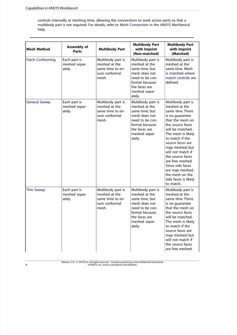
8/10/2019 ANSYS Meshing Users Guide
http://slidepdf.com/reader/full/ansys-meshing-users-guide 16/491
controls internally at meshing time, allowing the connections to work across parts so that amultibody part is not required. For details, refer to Mesh Connection in the ANSYS Mechanical
help.
Multibody Part
with Imprint
(Matched)
Multibody Part
with Imprint
(Non-matched)
Multibody PartAssembly of
Parts
Mesh Method
Multibody part ismeshed at the
Multibody part ismeshed at the
Multibody part ismeshed at the
Each part ismeshed separ-ately.
Patch Conforming
same time. Meshsame time, butsame time to en-is matched wheremesh does notsure conformal
mesh. match controls aredefined.
need to be con-formal becausethe faces aremeshed separ-
ately.
Multibody part is
meshed at the
Multibody part is
meshed at the
Multibody part is
meshed at the
Each part is
meshed separ-ately.
General Sweep
same time. Theresame time, butsame time to en-is no guaranteemesh does notsure conformal
mesh. that the mesh onneed to be con-
the source facesformal becausewill be matched.the faces are The mesh is likelymeshed separ-
ately. to match if the
source faces aremap meshed, butwill not match if
the source facesare free meshed.Since side facesare map meshed,
the mesh on theside faces is likelyto match.
Multibody part ismeshed at the
Multibody part ismeshed at the
Multibody part ismeshed at the
Each part ismeshed separ-ately.
Thin Sweep
same time. Theresame time, butsame time to en-
is no guaranteemesh does notsure conformalmesh. that the mesh onneed to be con-
the source facesformal becausewill be matched.the faces are
The mesh is likelymeshed separ-ately. to match if the
source faces are
map meshed, butwill not match if the source facesare free meshed.
Release 15.0 - © SAS IP, Inc. All rights reserved. - Contains proprietary and confidential informationof ANSYS, Inc. and its subsidiaries and affiliates.8
Capabilities in ANSYS Workbench
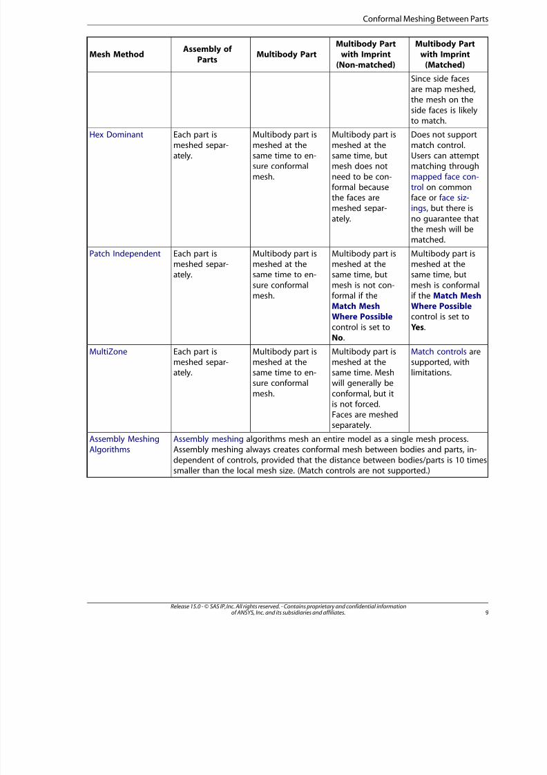
8/10/2019 ANSYS Meshing Users Guide
http://slidepdf.com/reader/full/ansys-meshing-users-guide 17/491
Multibody Partwith Imprint
(Matched)
Multibody Partwith Imprint
(Non-matched)Multibody Part
Assembly of
PartsMesh Method
Since side facesare map meshed,the mesh on the
side faces is likely
to match.Does not support
match control.
Multibody part is
meshed at the
Multibody part is
meshed at the
Each part is
meshed separ-ately.
Hex Dominant
Users can attemptsame time, butsame time to en-matching throughmesh does notsure conformal
mesh. mapped face con-need to be con-trol on commonformal becauseface or face siz-the faces areings, but there ismeshed separ-
ately. no guarantee thatthe mesh will be
matched.Multibody part ismeshed at the
Multibody part ismeshed at the
Multibody part ismeshed at the
Each part ismeshed separ-ately.
Patch Independent
same time, butsame time, butsame time to en-
mesh is conformalmesh is not con-sure conformalmesh. if the Match Meshformal if the
Where PossibleMatch Meshcontrol is set to
Yes.
Where Possible
control is set toNo.
Match controls are
supported, withlimitations.
Multibody part is
meshed at thesame time. Mesh
Multibody part is
meshed at thesame time to en-
Each part is
meshed separ-ately.
MultiZone
will generally besure conformal
mesh. conformal, but itis not forced.Faces are meshedseparately.
Assembly meshing algorithms mesh an entire model as a single mesh process.Assembly meshing always creates conformal mesh between bodies and parts, in-
Assembly MeshingAlgorithms
dependent of controls, provided that the distance between bodies/parts is 10 timessmaller than the local mesh size. (Match controls are not supported.)
9Release 15.0 - © SAS IP, Inc. All rights reserved. - Contains proprietary and confidential informationof ANSYS, Inc. and its subsidiaries and affiliates.
Conformal Meshing Between Parts

8/10/2019 ANSYS Meshing Users Guide
http://slidepdf.com/reader/full/ansys-meshing-users-guide 18/491
Release 15.0 - © SAS IP, Inc. All rights reserved. - Contains proprietary and confidential informationof ANSYS, Inc. and its subsidiaries and affiliates.10

8/10/2019 ANSYS Meshing Users Guide
http://slidepdf.com/reader/full/ansys-meshing-users-guide 19/491
Meshing: Usage in Workbench
The ANSYS Meshing application is a separate ANSYS Workbench application. The Meshing applicationis data-integrated with ANSYS Workbench, meaning that although the interface remains separate, thedata from the application communicates with the native ANSYS Workbench data. The following topics
are addressed in this section:Basic Meshing Application WorkflowsStrategies for CFD/Fluids Meshing in ANSYS Workbench
Accessing Meshing FunctionalityOverview of the Meshing Application InterfaceDetermination of Physics, Analysis, and Solver SettingsWorking with Legacy Mesh Data
Exporting Meshes or Faceted GeometryExtended ANSYS ICEM CFD MeshingWorking with Meshing Application ParametersANSYS Workbench and Mechanical APDL Application Meshing Differences
Basic Meshing Application Workflows
The following sections describe several basic workflows for using the Meshing application in ANSYS
Workbench:Overview of the Meshing Process in ANSYS WorkbenchOverview of the Meshing Process for CFD/Fluids AnalysesCombining CFD/Fluids Meshing and Structural Meshing
Overview of the Meshing Process in ANSYS Workbench
The following steps provide the basic workflow for using the Meshing application as part of an ANSYSWorkbench analysis (non-Fluid Flow). Refer to the ANSYS Workbench help for detailed informationabout working in ANSYS Workbench.
1. Select the appropriate template in the Toolbox, such as Static Structural . Double-click the template in
the Toolbox, or drag it onto the Project Schematic.
2. If necessary, define appropriate engineering data for your analysis. Right-click the Engineering Data celand select Edit, or double-click the Engineering Data cell. The Engineering Data workspace appears,
where you can add or edit material data as necessary.
3. Attach geometry to your system or build new geometry in the ANSYS DesignModeler application. Righclick the Geometry cell and select Import Geometry... to attach an existing model or select New Geo-metry... to launch the DesignModeler application.
4. Access the Meshing application functionality. Right-click the Model cell and choose Edit. This step willlaunch the ANSYS Mechanical application.
1Release 15.0 - © SAS IP, Inc. All rights reserved. - Contains proprietary and confidential informationof ANSYS, Inc. and its subsidiaries and affiliates.
8/10/2019 ANSYS Meshing Users Guide
http://slidepdf.com/reader/full/ansys-meshing-users-guide 20/491
5. Once you are in the Mechanical application, you can move between its components by highlighting thecorresponding object in the Tree as needed. Click on the Mesh object in the Tree to access Meshing
application functionality and apply mesh controls.
6. Define loads and boundary conditions. Right-click the Setup cell and select Edit. The appropriate applic-ation for your selected analysis type will open (such as the Mechanical application). Set up your analysis
using that application's tools and features.
7. You can solve your analysis by issuing an Update, either from the data-integrated application you're usingto set up your analysis, or from the ANSYS Workbench GUI.
8. Review your analysis results.
Note
You should save your data periodically (File> Save Project). The data will be saved as a.wbpj file. Refer to the ANSYS Workbench help for more information about project file
management in Workbench.
For more information:
• For information on identifying and correcting mesh failures, refer to "Meshing: Troubleshooting" (p. 391).
• For information about using the ANSYS Meshing application to import or export mesh files, refer toWorking with Legacy Mesh Data (p. 21) and Exporting Meshes or Faceted Geometry (p. 23).
• Fluids users of the ANSYS DesignModeler, ANSYS Meshing, and ANSYS CFX applications should referto "Meshing: Named Selections and Regions for ANSYS CFX" (p. 389) for important information aboutregion definitions.
• Fluids users of the ANSYS DesignModeler, ANSYS Meshing, and ANSYS Fluent applications should
refer to Fluent Mesh Export (p. 24) for important information about Named Selection support.
Overview of the Meshing Process for CFD/Fluids Analyses
This section describes the basic process for using the ANSYS Meshing application to create a mesh aspart of an ANSYS Workbench CFD/fluids analysis. Refer to Strategies for CFD/Fluids Meshing in ANSYSWorkbench (p. 15) for information about different CFD/Fluids meshing strategies. Refer to the ANSYS
Workbench help for detailed information about working in ANSYS Workbench. There are four basicsteps to creating a mesh:
Create Geometry
You can create geometry for the Meshing application from scratch in the ANSYS DesignModeler applic-ation, or import it from an external CAD file. The Meshing application requires you to construct solid
bodies (not surface bodies) to define the region for the 3D mesh (for 2D simulations a sheet body canbe used). A separate body must be created for each region of interest in the fluids simulation; for example,a region in which you want the fluids solver to solve for heat transfer only must be created as a separatebody. Multiple bodies are created in the DesignModeler application by using the Freeze command; see
Freeze in the DesignModeler help for details.
It is best practice to explicitly identify any fluid regions in the model as fluids rather than solids.
Release 15.0 - © SAS IP, Inc. All rights reserved. - Contains proprietary and confidential informationof ANSYS, Inc. and its subsidiaries and affiliates.12
Usage in Workbench
8/10/2019 ANSYS Meshing Users Guide
http://slidepdf.com/reader/full/ansys-meshing-users-guide 21/491
For new users or new models it is often useful to first generate a default mesh, evaluate it, and thenapply the controls described in Define Mesh Attributes (p. 13) as appropriate to improve various mesh
characteristics.
Define Named Selections
During the fluids simulation setup, you will need to define boundary conditions where you can applyspecific physics. For example, you may need to define where the fluid enters the geometry or where itexits. Although it may be possible to select the faces that correspond to a particular boundary condition
inside the solver application, it is rather easier to make this selection ahead of time in either the CADconnection, the ANSYS DesignModeler application, or the Meshing application. In addition, it is muchbetter to define the location of periodic boundaries before the mesh is generated to allow the nodes
of the surface mesh to match on the two sides of the periodic boundary, which in turn allows for amore accurate fluids solution. You can define the locations of boundaries by defining Named Selections,which can assist you in the following ways:
• You can use Named Selections to easily hide the outside boundary in an external flow problem.
• You can assign Named Selections to all faces in a model except walls, and Program Controlled inflationwill automatically select all walls in the model to be inflation boundaries.
For more information:
• Fluids users of the ANSYS DesignModeler, ANSYS Meshing, and ANSYS CFX applications should referto "Meshing: Named Selections and Regions for ANSYS CFX" (p. 389).
• Fluids users of the ANSYS DesignModeler, ANSYS Meshing, and ANSYS Fluent applications should
refer to Fluent Mesh Export (p. 24).
Define Mesh Attributes
The mesh generation process in the Meshing application is fully automatic. However, you have consid-
erable control over how the mesh elements are distributed. To ensure that you get the best fluidssolution possible with your available computing resources, you can dictate the background element
size, type of mesh to generate, and where and how the mesh should be refined. In general, setting upthe length scale field for your mesh is a three-step process, as outlined below:
• Assign a suitable set of global mesh controls.
• Override the default mesh type by inserting a different mesh method.
• Override the global sizing or other controls locally on bodies, faces, edges, or vertices and the regionsclose to them by scoping local mesh controls.
Generate Mesh
When you are ready to compute the mesh, you can do so by using either the Update feature or the
Generate Mesh feature. Either feature computes the entire mesh. The surface mesh and the volumemesh are generated at one time. The mesh for all parts/bodies is also generated at one time. For helpin understanding the difference between the Update and Generate Mesh features, see Updating the
Mesh Cell State (p. 353).
13Release 15.0 - © SAS IP, Inc. All rights reserved. - Contains proprietary and confidential informationof ANSYS, Inc. and its subsidiaries and affiliates.
Basic Meshing Application Workflows
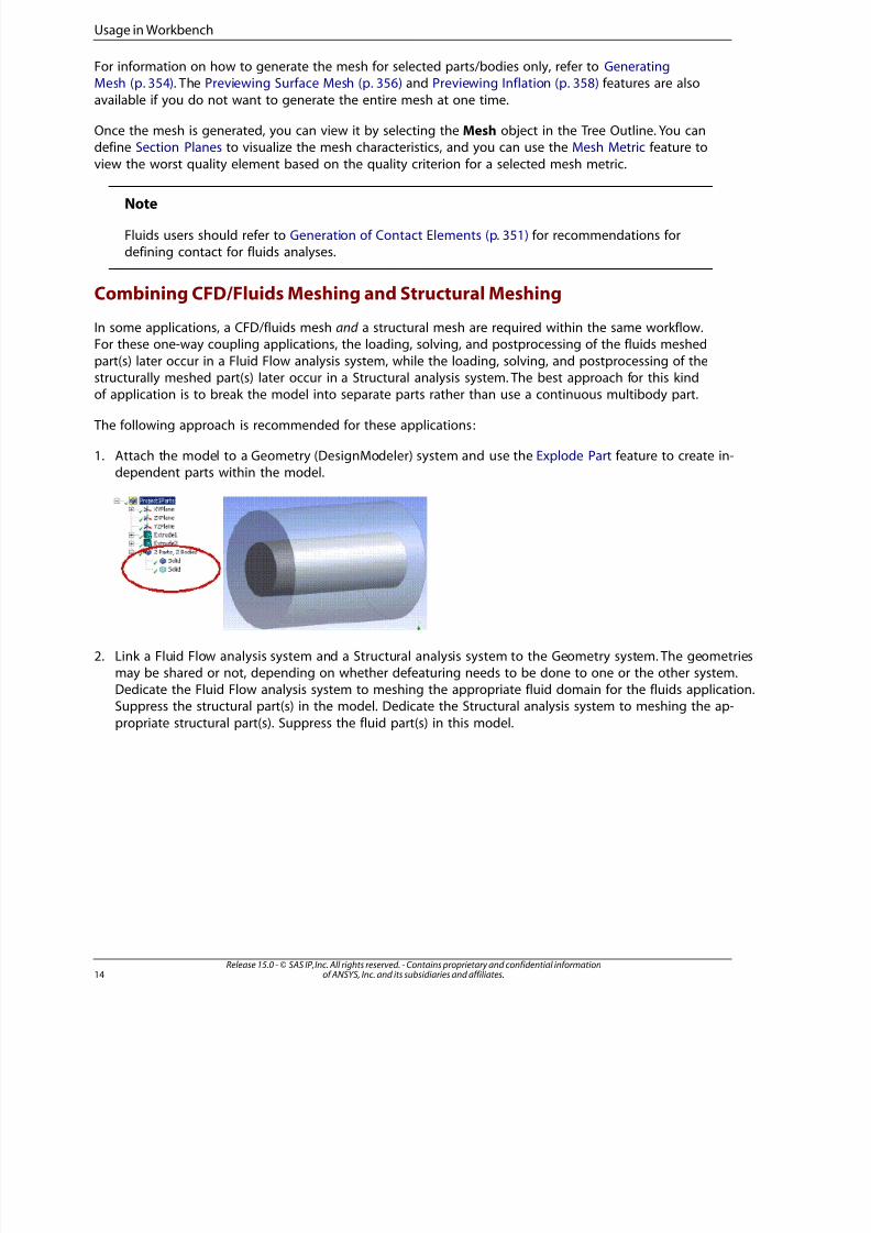
8/10/2019 ANSYS Meshing Users Guide
http://slidepdf.com/reader/full/ansys-meshing-users-guide 22/491
For information on how to generate the mesh for selected parts/bodies only, refer to GeneratingMesh (p. 354). The Previewing Surface Mesh (p. 356) and Previewing Inflation (p. 358) features are also
available if you do not want to generate the entire mesh at one time.
Once the mesh is generated, you can view it by selecting the Mesh object in the Tree Outline. You candefine Section Planes to visualize the mesh characteristics, and you can use the Mesh Metric feature to
view the worst quality element based on the quality criterion for a selected mesh metric.
Note
Fluids users should refer to Generation of Contact Elements (p. 351) for recommendations fordefining contact for fluids analyses.
Combining CFD/Fluids Meshing and Structural Meshing
In some applications, a CFD/fluids mesh and a structural mesh are required within the same workflow.For these one-way coupling applications, the loading, solving, and postprocessing of the fluids meshed
part(s) later occur in a Fluid Flow analysis system, while the loading, solving, and postprocessing of thestructurally meshed part(s) later occur in a Structural analysis system. The best approach for this kindof application is to break the model into separate parts rather than use a continuous multibody part.
The following approach is recommended for these applications:
1. Attach the model to a Geometry (DesignModeler) system and use the Explode Part feature to create in-dependent parts within the model.
2. Link a Fluid Flow analysis system and a Structural analysis system to the Geometry system. The geometriesmay be shared or not, depending on whether defeaturing needs to be done to one or the other system.Dedicate the Fluid Flow analysis system to meshing the appropriate fluid domain for the fluids application.Suppress the structural part(s) in the model. Dedicate the Structural analysis system to meshing the ap-
propriate structural part(s). Suppress the fluid part(s) in this model.
Release 15.0 - © SAS IP, Inc. All rights reserved. - Contains proprietary and confidential informationof ANSYS, Inc. and its subsidiaries and affiliates.14
Usage in Workbench
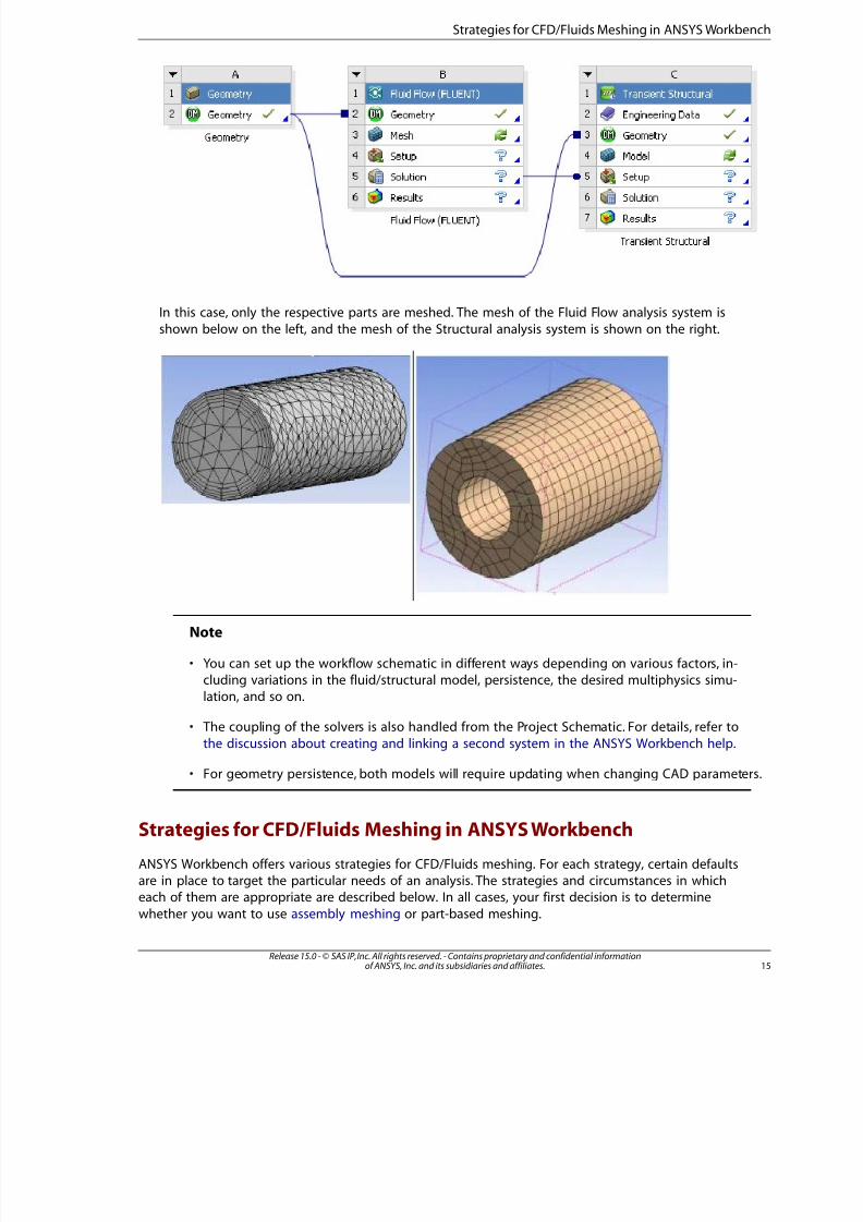
8/10/2019 ANSYS Meshing Users Guide
http://slidepdf.com/reader/full/ansys-meshing-users-guide 23/491
In this case, only the respective parts are meshed. The mesh of the Fluid Flow analysis system is
shown below on the left, and the mesh of the Structural analysis system is shown on the right.
Note
• You can set up the workflow schematic in different ways depending on various factors, in-cluding variations in the fluid/structural model, persistence, the desired multiphysics simu-lation, and so on.
• The coupling of the solvers is also handled from the Project Schematic. For details, refer to
the discussion about creating and linking a second system in the ANSYS Workbench help.
• For geometry persistence, both models will require updating when changing CAD parameters.
Strategies for CFD/Fluids Meshing in ANSYS Workbench
ANSYS Workbench offers various strategies for CFD/Fluids meshing. For each strategy, certain defaultsare in place to target the particular needs of an analysis. The strategies and circumstances in whicheach of them are appropriate are described below. In all cases, your first decision is to determine
whether you want to use assembly meshing or part-based meshing.
15Release 15.0 - © SAS IP, Inc. All rights reserved. - Contains proprietary and confidential informationof ANSYS, Inc. and its subsidiaries and affiliates.
Strategies for CFD/Fluids Meshing in ANSYS Workbench

8/10/2019 ANSYS Meshing Users Guide
http://slidepdf.com/reader/full/ansys-meshing-users-guide 24/491
Tetra Dominant Meshing - Patch Conforming Tetra/Prism Meshing
The first strategy is to use conformal tetra/prism meshing plus the default Sweep method. This strategyis recommended for models involving moderately clean CAD (for example, native CAD, Parasolid, ACIS,and so on) for which you desire a tetra/hybrid dominant mesh.
Although the Patch Conforming Tetra mesh method is fully automated, it interacts with additional meshcontrols and capabilities as necessary, including:
• Advanced tetra and inflation layer technology
• Pinch controls for removing small features at the mesh level (offered as an alternative to Virtual To-pologies, which work at the geometry level)
• Advanced Size Function controls for providing greater control over mesh distribution
• Conformal swept regions
• Body of influence (BOI) for setting one body as a size source for another body
Tetra Dominant Meshing - Patch Independent Tetra/Prism Meshing
An alternative for those desiring a tetra dominant mesh is Patch Independent Tetra /Prism meshing. This approach is best for "dirty CAD"—CAD models with many surface patches (for example, IGES, CATIA
V4, and so on) and in cases with large numbers of slivers/small edges/sharp corners. It includes supportfor post inflation, as well as CAD simplification built-in to the tetra mesher.
Mapped Hex Meshing - All Hex Swept Meshing
This mapped hex approach (which includes both general Sweep and thin Sweep) is recommended forclean CAD. It supports single source to single target volumes, and may require you to perform manualgeometry decomposition.
Benefits of this approach include:
• Support for Advanced Size Function controls
• Compatibility with Patch Conforming Tetra meshing
• Support for swept inflation
Mapped and Free Meshing - MultiZone Meshing
Best for moderately clean CAD, the MultiZone strategy for meshing provides multi-level sweep with
automatic decomposition of geometry into mapped (structured) and free (unstructured) regions. Whendefining the MultiZone mesh method, you can specify a Mapped Mesh Type and a Free Mesh Type
that will be used to fill structured and unstructured regions respectively. Depending on your settingsand specific model, the mesh may contain a mixture of hex/prism/tetra elements.
The MultiZone mesh method and the Sweep mesh method described above operate similarly; however,
MultiZone has capabilities that make it more suitable for a class of problems for which the Sweepmethod would not work without extensive geometry decomposition.
Additional benefits of this approach include:
Release 15.0 - © SAS IP, Inc. All rights reserved. - Contains proprietary and confidential informationof ANSYS, Inc. and its subsidiaries and affiliates.16
Usage in Workbench
8/10/2019 ANSYS Meshing Users Guide
http://slidepdf.com/reader/full/ansys-meshing-users-guide 25/491
• Support for 3D inflation
• Ability to selectively ignore small features
Assembly Meshing - CutCell and Tetrahedrons Algorithms
CutCell Cartesian meshing is a general purpose assembly meshing algorithm designed for ANSYS Fluent.
CutCell is in principal a Patch Independent mesher, and it is mostly suitable for moderately clean CADmodels. It results in a mesh of 80-95% hex cells, which often leads to very accurate solutions, providingthe physics can handle the relatively rapid size changes due to hanging-node configurations.
Additional benefits of this approach include:
• Support for Advanced Size Function controls
• Support for 3D inflation, although very thick inflation should be avoided when using the CutCell al-
gorithm
• Ability to selectively ignore features
The Tetrahedrons assembly meshing algorithm is a derivative of the CutCell algorithm, with strengths
and weaknesses similar to those of CutCell. The Tetrahedrons method starts from the CutCell mesh andthrough various mesh manipulations creates a high quality unstructured tet mesh.
Accessing Meshing Functionality
You can access Meshing application functionality from the Model/Mesh cell in an analysis system, orfrom the Mesh cell in a Mesh component system. Before using the steps provided in this section, youshould be familiar with the concepts of analysis systems and component systems in ANSYS Workbench.
Accessing Meshing Functionality from an Analysis System
The Model cell (Mesh cell in Fluid Flow analysis systems) allows you to access a meshing application or
share a mesh with another system. Model corresponds to the contents of the Model branch within theANSYS Mechanical application and allows you to perform physics-based meshing capabilities, such asspot welds, contact, etc. Mesh contains just node coordinates and mesh connectivity.
To launch the Meshing application from a Model cell in an analysis system (non-Fluid Flow):
1. From the Analysis Systems group of the ANSYS Workbench Toolbox, either double-click or drag an ana-lysis system onto the Project Schematic. As a result, a template for that type of analysis system appearsin the Project Schematic.
2. In the analysis system, right-click on the Geometry cell and choose New Geometry to create geometrywithin the ANSYS DesignModeler application, or choose Import Geometry to attach existing geometry
3. Right-click the Model cell and choose Edit. This step will launch the Mechanical application. From the
Mechanical application, you can access the Meshing application controls by clicking on the Mesh objecin the Tree Outline.
To access meshing from a Mesh cell in a Fluid Flow analysis system:
17Release 15.0 - © SAS IP, Inc. All rights reserved. - Contains proprietary and confidential informationof ANSYS, Inc. and its subsidiaries and affiliates.
Accessing Meshing Functionality
8/10/2019 ANSYS Meshing Users Guide
http://slidepdf.com/reader/full/ansys-meshing-users-guide 26/491
1. From the Analysis Systems group of the ANSYS Workbench Toolbox, either double-click or drag a FluidFlow analysis system onto the Project Schematic. As a result, a template for that type of analysis system
appears in the Project Schematic.
2. In the analysis system, right-click on the Geometry cell and choose New Geometry to create geometrywithin the DesignModeler application, or choose Import Geometry to attach existing geometry.
3. Right-click the Mesh cell and choose Edit. This step will launch the appropriate mesh application (e.g.,
the Meshing application, etc.).
Accessing Meshing Functionality from a Mesh Component System
To launch the Meshing application from a Mesh component system:
1. From the Component Systems group of the ANSYS Workbench Toolbox, either double-click or drag a
Mesh component system onto the Project Schematic. As a result, a template of a Mesh system appearsin the Project Schematic.
2. In the Mesh system, right-click on the Geometry cell and choose New Geometry to create geometry
within the ANSYS DesignModeler application, or choose Import Geometry to attach existing geometry.
3. Right-click the Mesh cell and choose Edit. This step will launch the appropriate mesh application (e.g.,the Meshing application, etc.).
Replacing a Mesh System with a Mechanical Model System
You can replace a Mesh component system with a Mechanical Model component system. This systemcan then be shared with any analysis system. For details, refer to the description of Mechanical Model
systems in the ANSYS Workbench help.
Overview of the Meshing Application Interface
The intuitive Meshing application interface, which is shown in Figure 1: Meshing Application Inter-face (p. 19), facilitates your use of all meshing controls and settings.
Release 15.0 - © SAS IP, Inc. All rights reserved. - Contains proprietary and confidential informationof ANSYS, Inc. and its subsidiaries and affiliates.18
Usage in Workbench
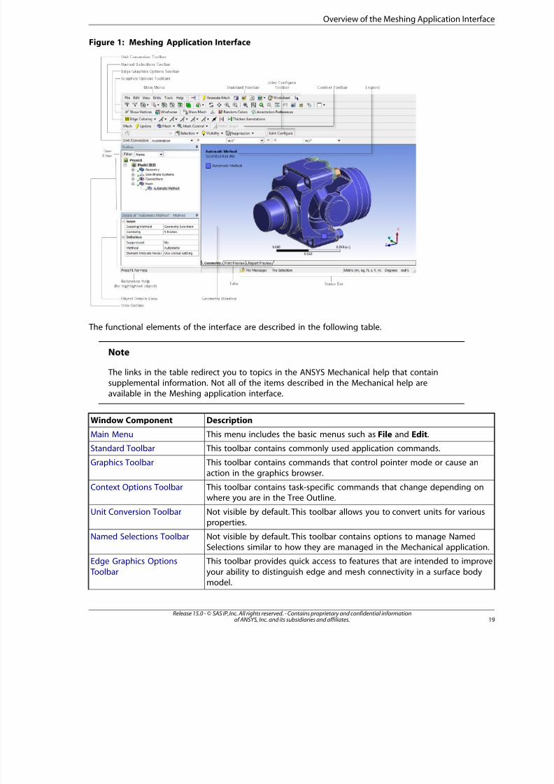
8/10/2019 ANSYS Meshing Users Guide
http://slidepdf.com/reader/full/ansys-meshing-users-guide 27/491
Figure 1: Meshing Application Interface
The functional elements of the interface are described in the following table.
Note
The links in the table redirect you to topics in the ANSYS Mechanical help that containsupplemental information. Not all of the items described in the Mechanical help areavailable in the Meshing application interface.
DescriptionWindow Component
This menu includes the basic menus such as File and Edit.Main Menu
This toolbar contains commonly used application commands.Standard Toolbar
This toolbar contains commands that control pointer mode or cause anaction in the graphics browser.
Graphics Toolbar
This toolbar contains task-specific commands that change depending onwhere you are in the Tree Outline.
Context Options Toolbar
Not visible by default. This toolbar allows you to convert units for variousproperties.
Unit Conversion Toolbar
Not visible by default. This toolbar contains options to manage NamedSelections similar to how they are managed in the Mechanical application.
Named Selections Toolbar
This toolbar provides quick access to features that are intended to improve
your ability to distinguish edge and mesh connectivity in a surface bodymodel.
Edge Graphics Options
Toolbar
19Release 15.0 - © SAS IP, Inc. All rights reserved. - Contains proprietary and confidential informationof ANSYS, Inc. and its subsidiaries and affiliates.
Overview of the Meshing Application Interface
8/10/2019 ANSYS Meshing Users Guide
http://slidepdf.com/reader/full/ansys-meshing-users-guide 28/491
DescriptionWindow Component
Outline view of the project. Always visible. Location in the outline sets thecontext for other controls. Provides access to object's context menus. Allows
renaming of objects. Establishes what details display in the Details View.
Tree Outline
The Details View corresponds to the Outline selection. Displays a details
window on the lower left panel which contains details about each objectin the Outline.
Details View
Displays and manipulates the visual representation of the object se-
lected in the Outline. This window may display:
Geometry Window (also
sometimes called theGraphics window)
• 3D Geometry
• 2D/3D Graph
• Spreadsheet
• HTML Pages
• Scale ruler
• Triad control
• Legend
Note
• Hover your mouse over the time stamp in the legend and
RMB click to toggle the time stamp off and on.
• The Geometry window may include splitter bars for dividingviews.
Opens an objects reference help page for the highlighted object. Theseare the same pages that are available in the Mechanical application.
Reference Help
The document tabs that are visible on the lower right portion of the win-dow.
Tabs
Brief in-context tip. Selection feedback.Status Bar
Application window has up to 3 splitter bars.Splitter Bar
Determination of Physics, Analysis, and Solver SettingsMost systems in ANSYS Workbench are defined by three primary attributes: physics type, analysis type,and solver type. The method you use to launch the Meshing application functionality determines howdefault physics, analysis, and/or solver settings are defined:
• Mesh systems, which are a type of component system, are unfiltered (physics, analysis, and solver).
If you launch the Meshing application from a Mesh component system, your preferences will be setto the defaults you previously defined within the Meshing application. See Meshing Overview (p. 1)for more information.
Release 15.0 - © SAS IP, Inc. All rights reserved. - Contains proprietary and confidential informationof ANSYS, Inc. and its subsidiaries and affiliates.20
Usage in Workbench

8/10/2019 ANSYS Meshing Users Guide
http://slidepdf.com/reader/full/ansys-meshing-users-guide 29/491
• If you launch the Meshing application from an analysis system (whether it be via the Model cell in anon-Fluid Flow analysis system or the Mesh cell in a Fluid Flow analysis system), your Physics, Analysis,
and Solver settings will be set according to the selected type of analysis system. To change thePhysics Preference, you must use the Details View of the Mesh folder.
Note
• To view the physics, analysis, and solver types that are defined for an analysis system,right-click the Model cell (non-Fluid Flow analyses) or Mesh cell (Fluid Flow analyses) andselect Properties. This step will open the Properties window, where you can view the at-tributes. For example, for an Electric system, the Properties window will show that Physicsis Electric, Analysis is Steady-State Electric Conduction, and Solver is Mechanical APDL.
• Mechanical Model systems, which are a type of component system, are unfiltered (physicsand solver). For details, refer to the discussion of Mechanical Model systems in the ANSYSWorkbench help.
For more information:
• For a list of analysis systems available in ANSYS Workbench and basic steps for building each typeof system, refer to the discussion of analysis systems in the ANSYS Workbench help.
• For details about the various types of non-Fluid Flow analyses and how to perform them, refer to thediscussion of analysis types in the ANSYS Mechanical help.
• For details about Fluid Flow analyses and how to perform them, refer to the documentation availableunder the Help menu within ANSYS CFX or ANSYS Fluent.
Working with Legacy Mesh Data
You can import legacy mesh files using the following methods. The method that is best for you dependson the type of file that you want to import and how you intend to use it:
• Choose File> Import from the ANSYS Workbench Menu bar or click the Import button on the ANSYSWorkbench Toolbar to read legacy ANSYS Workbench mesh data
• Right-click the Mesh cell and choose Import Mesh File to import a read-only mesh for downstreamuse
• Use the FE Modeler system to read a legacy mesh input file for reuse as a mesh or geometry forother ANSYS Workbench systems
Importing Using File> Import or the Import Button
If you choose File> Import or click the Import button from ANSYS Workbench, you can import mesh
files that have an extension of .cmdb or .meshdat. Doing so creates a Mesh system in the ANSYSWorkbench Project Schematic. When the Mesh cell is edited, the mesh will open in the Meshing applic-ation where you can edit it.
2Release 15.0 - © SAS IP, Inc. All rights reserved. - Contains proprietary and confidential informationof ANSYS, Inc. and its subsidiaries and affiliates.
Working with Legacy Mesh Data
8/10/2019 ANSYS Meshing Users Guide
http://slidepdf.com/reader/full/ansys-meshing-users-guide 30/491
For more information about reading a simulation/mesh database (.dsdb/.cmdb) from previous ANSYSversions, please refer to the discussion of importing legacy databases in the ANSYS Workbench help.
Note
ANSYS Workbench no longer supports the CFX-Mesh method. Upon import of a legacymodel into Release 15.0, any CFX-Mesh method controls will be made inoperable, and you
must either delete the method manually or change it to a valid method type. If importing a*.cmdb file from Release 10.0 that contains CFX-Mesh data, please first take the model intoRelease 11.0 and save it to convert it to a supported format for use in Release 15.0. In eithercase the geometry will be maintained, but the mesh method must be replaced.
Importing Read-only Meshes for Downstream Application Use
You can right-click a Mesh cell and choose Import Mesh File to browse to a mesh file that you wantto import, provided the file is of one of the following types:
• ANSYS CFX mesh file with extension .gtm or .cfx
• ANSYS ICEM CFD mesh file with extension .cfx, cfx5, or .msh
• ANSYS Fluent mesh file with extension .cas, .msh, or .gz
• ANSYS Polyflow mesh file with extension .poly, .neu, or .msh
Note
When you use this method, in the strictest sense you are not “importing” the mesh file. Thatis, you will not be able to edit the file in the Meshing application using this method. Rather,
you are making the mesh available for downstream systems. To be able to edit these types
of files in the Meshing application, you must import the mesh into the FE Modeler application,and then into another system. Refer to Importing Legacy Meshes for Edit Using FE Model-er (p. 23).
The Import Mesh File method is enabled when:
• No geometry is associated with the Geometry cell.
• No generated mesh is associated with the Mesh cell. (Imported meshes do not disable the Import
Mesh File menu item.)
• No incoming connections are associated with the Geometry cell or Mesh cell.
• No outgoing connections are associated with the Geometry cell.
• No outgoing connections from the Mesh cell are connected to the FE Modeler, Mechanical APDL, orANSYS Autodyn applications.
When you import the mesh to the Mesh cell:
• The Geometry cell is deleted.
• The title of the cell changes from “Mesh” to “Imported Mesh.”
Release 15.0 - © SAS IP, Inc. All rights reserved. - Contains proprietary and confidential informationof ANSYS, Inc. and its subsidiaries and affiliates.22
Usage in Workbench
8/10/2019 ANSYS Meshing Users Guide
http://slidepdf.com/reader/full/ansys-meshing-users-guide 31/491
• The state of the Mesh cell is “Up to Date.”
• No incoming connections are allowed.
• Outgoing connections can be established with a Mechanical APDL, ANSYS Autodyn, ANSYS CFX,ANSYS Fluent, ANSYS Polyflow, or FE Modeler system.
• The Geometry cell in the target system is deleted.
• Using the reset command (right-clicking on the Imported Mesh cell and choosing Reset) deletes theimported mesh.
Importing Legacy Meshes for Edit Using FE Modeler
You can import a legacy mesh for the purposes of editing it in the Meshing application, but the meshmust come from an FE Modeler system. This is necessary because before it can be imported into the
Meshing application to edit, the mesh must be associated with a geometry. The FE Modeler applicationallows you to import a mesh and create a geometry that will be associated with that mesh. For moreinformation, please see the FE Modeler help.
After you use an FE Modeler system to import a mesh and create a geometry from it, you must connectan analysis system, Mechanical Model system, or Mesh system to the FE Modeler system. When thisfollow-on system is edited, the mesh will open in the Meshing application.
Exporting Meshes or Faceted Geometry
A mesh generated by the Meshing application can be exported into the following file formats:
• Meshing File format (*.meshdat), suitable for import into ANSYS Workbench
• ANSYS Fluent mesh format (*.msh), suitable for import into ANSYS Fluent
• ANSYS Polyflow format (*.poly), suitable for import into ANSYS Polyflow
• CGNS format (*.cgns), suitable for import into a CGNS-compatible application
• ANSYS ICEM CFD format (*.prj), suitable for import into ANSYS ICEM CFD
To export a mesh:
1. Generate the mesh.
2. Select File> Export from the main menu.
3. In the Save As dialog box, choose a directory and specify a file name for the file. Then choose a file typfrom the Save as type drop-down menu and click Save.
Note
• You can also use the Meshing application to export faceted geometry for use in ANSYS FluentMeshing. In such cases you can skip step 1 above. A file with the extension .tgf is created,suitable for import into ANSYS Fluent Meshing.
23Release 15.0 - © SAS IP, Inc. All rights reserved. - Contains proprietary and confidential informationof ANSYS, Inc. and its subsidiaries and affiliates.
Exporting Meshes or Faceted Geometry

8/10/2019 ANSYS Meshing Users Guide
http://slidepdf.com/reader/full/ansys-meshing-users-guide 32/491
• When the same entity is a member of more than one Named Selection, those Named Selectionsare said to be “overlapping.” If you are exporting a mesh into the ANSYS Fluent, ANSYS Polyflow,
CGNS, or ANSYS ICEM CFD format (or faceted geometry into the ANSYS Fluent Meshing format),and overlapping Named Selections are detected, the export will fail and you must resolve theoverlapping Named Selections before proceeding. For details, see Showing Geometry in Over-lapping Named Selections (p. 361).
For details, refer to:Mesh Application File ExportFluent Mesh Export
Polyflow ExportCGNS ExportANSYS ICEM CFD ExportExporting Faceted Geometry to TGrid (ANSYS Fluent Meshing)
Mesh Application File Export
When you export a mesh file to Meshing File format (File> Export from the Meshing application main
menu, then Save as type Meshing File), a file with the extension .meshdat is created. The exportedfile can be imported as a legacy file into ANSYS Workbench by either selecting File >Import from theMenu bar or clicking the Import button on the Toolbar, and then selecting an Importable Mesh File.
This will create a Mesh System in the ANSYS Workbench Project Schematic.
Fluent Mesh Export
When you export a mesh file to ANSYS Fluent mesh format (File> Export from the Meshing applicationmain menu, then Save as type Fluent Input Files), a mesh file with the extension .msh is created. Theexported mesh file is suitable for import into another product such as ANSYS Fluent, or into ANSYSFluent Meshing outside of ANSYS Workbench. For more control over the input file, refer to Meshing
Options on the Options Dialog Box (p. 225).
CutCell meshes exported from the Meshing application are always in polyhedral format. When readinto ANSYS Fluent Meshing, it will skip the polyhedral cells.
If the mesh file you export contains quadratic elements, all midside nodes will be dropped during export;that is, all element types will be exported as linear element types for ANSYS Fluent.
An orientation check/correction will be performed for 3D geometry models exported as 2D mesh such
that all 2D cells will have the same orientation. You do not need to manually correct the orientation of the geometry face(s).
When the mesh file is exported to ANSYS Fluent mesh format, the material properties of the bodies/partsin the model must be translated to proper continuum zone types for use in ANSYS Fluent. To provide
this information to ANSYS Fluent, the following logic is used:
Release 15.0 - © SAS IP, Inc. All rights reserved. - Contains proprietary and confidential informationof ANSYS, Inc. and its subsidiaries and affiliates.24
Usage in Workbench
8/10/2019 ANSYS Meshing Users Guide
http://slidepdf.com/reader/full/ansys-meshing-users-guide 33/491
1. If Physics Preference (p. 65) is set to CFD and you do not use either of the methods described insteps 2 or 3 below to explicitly assign a body/part to be either solid or fluid, all zones are exported
to ANSYS Fluent mesh format as FLUID zones by default.
Note
An exception to the above involves models that include an enclosure. If you used
the Enclosure feature in the ANSYS DesignModeler application, the enclosure bodywill be assigned a continuum zone type of FLUID by default.
2. For models created/edited in the DesignModeler application, a Fluid/Solid material property canbe assigned to a solid body or a multibody part (if the multibody part contains at least one solidbody). This material assignment appears under Details of Body in the Details View of the Design-
Modeler application.
For multibody parts, you can change the material property for all bodies in one operation inthe DesignModeler application by modifying the Fluid/Solid property for the multibody part
and the modification will propagate to any solid bodies in the part. Similarly, you can use the
DesignModeler application to modify the Fluid/Solid property for a solid body that belongsto a multibody part, and the Fluid/Solid property for the multibody part will be modified ac-cordingly.
When exported to TGrid format, a body/part with a material property of Solid will be assigneda continuum zone type of SOLID and a body/part with a material property of Fluid will be as-signed a continuum zone type of FLUID. This setting in the DesignModeler application overrides
the default behavior described in step 1.
Note
Refer to Figure 3: Multibody Part Containing All Fluid Bodies in the DesignModelerApplication (p. 36) for an example that illustrates where to set the Fluid/Solid ma-terial property in the DesignModeler application.
3. Finally, the Fluid/Solid material property setting in the Meshing application is considered. Thismaterial assignment appears in the Details View of the Meshing application when a prototype (i.e.,Body object) is selected in the Tree Outline. Similar to the DesignModeler application feature de-
scribed in step 2, the Meshing application lets you change the Fluid/Solid material property for abody.
When exported to ANSYS Fluent mesh format, a body with a material property of Solid will be
assigned a continuum zone type of SOLID and a body with a material property of Fluid will beassigned a continuum zone type of FLUID. This setting in the Meshing application overridesany assignments that were made based on the default behavior described in step 1 or the
25Release 15.0 - © SAS IP, Inc. All rights reserved. - Contains proprietary and confidential informationof ANSYS, Inc. and its subsidiaries and affiliates.
Exporting Meshes or Faceted Geometry

8/10/2019 ANSYS Meshing Users Guide
http://slidepdf.com/reader/full/ansys-meshing-users-guide 34/491
Fluid/Solid setting described in step 2. Refer to Changing Fluid/Solid Material Property Set-tings (p. 283) for more information.
Note
If there are multiple continuum zones or boundary zones of the same type in theDesignModeler application or the Meshing application, each zone name in the exported
ANSYS Fluent mesh file will contain the necessary prefix and an arbitrary number willbe appended to the name to make it unique. Refer to Examples of Fluent Mesh Export:An Alternative to Using a Fluid Flow (Fluent) Analysis System (p. 35) for an examplethat illustrates multiple zones of the same type.
For related information, refer to:
Classes of Zone Types in ANSYS FluentStandard Naming Conventions for Naming Named SelectionsZone Type AssignmentExamples of Fluent Mesh Export: An Alternative to Using a Fluid Flow (Fluent) Analysis System
Note
• Contact regions are said to be “overlapping” when the same entity is a member of more thanone contact region or when multiple contact regions share the same geometry. ANSYS Fluentdoes not support overlapping contact regions. For part-based meshing only, if you are exporting
a mesh into the ANSYS Fluent format and overlapping contact regions are detected, the exportwill fail and you must resolve the overlapping contact regions before proceeding. If available,an option to show the overlapping contact regions is shown. For details, see Showing Geometryin Overlapping Contact Regions (p. 361).
• Changes in Release 14.5 affect mesh interface handling during export to ANSYS Fluent. For thisreason, you may receive an error message after resuming a Release 14.0 project in which a
mesh generated in the Meshing application was exported to ANSYS Fluent. Specifically, whenyou try to Update the Mesh cell, you may receive an error message indicating the mesh fileexporter failed. To correct the problem, you can Reset the Mesh cell, define the mesh sizesand controls, and then Update the Mesh cell.
• If you are performing a 2D analysis and intend to export to ANSYS Fluent, you should disable
the Auto Detect Contact On Attach option to avoid problems that may otherwise occur uponexport. You can access this option by selecting Tools> Options from the ANSYS Workbenchmain menu, and then selecting either the Mechanical or Meshing category as appropriate. The
option is enabled by default in both applications.
• For additional information about importing files into ANSYS Fluent or ANSYS Fluent Meshing,
refer to the documentation available under the Help menu within the respective product.
Classes of Zone Types in ANSYS Fluent
Zone type specifications in ANSYS Fluent define the physical and operational characteristics of the
model at its boundaries and within specific regions of its domain. There are two classes of zone typespecifications:
• Boundary zone types (sometimes called “face zones”)
Release 15.0 - © SAS IP, Inc. All rights reserved. - Contains proprietary and confidential informationof ANSYS, Inc. and its subsidiaries and affiliates.26
Usage in Workbench
8/10/2019 ANSYS Meshing Users Guide
http://slidepdf.com/reader/full/ansys-meshing-users-guide 35/491
• Continuum zone types (sometimes called “cell zones”)
Boundary zone type specifications, such as WALL or INLET_VENT , define the characteristics of the modelat its external or internal boundaries. Boundary zones are collections of faces in 3D, and collections of edges in 2D. By default, a boundary zone of type WALL is created for the boundary of each body in thegeometry during export to ANSYS Fluent mesh format. Continuum zone type specifications, such as
FLUID or SOLID, define the characteristics of the model within specified regions of its domain. By default,a continuum zone is created for each body in the geometry during export to ANSYS Fluent mesh format.
(By default, continuum zone types will be assigned as described in Fluent Mesh Export (p. 24).)
If you do not want the default zone type to be assigned to a boundary zone, you can set the Auto Zone Type Assignment option to Off . You can then override default type of WALL by defining Named Selectionsand naming them according to the conventions provided. All faces belonging to the same body in aNamed Selection are placed into a single boundary zone.
Note
For 2D models, you can group sheet surface bodies into a Named Selection, and the under-lying faces contained in the sheet surface bodies will be placed into a single continuum zone
(as long as the faces themselves are not contained in a Named Selection).
The following sections further describe boundary zone type and continuum zone type specifications
and illustrate their purposes in the definition of an example computational model involving simplegeometry.
For details on how zones are named and how zone types are assigned during export, refer to Zone
Type Assignment (p. 30).
For an example that illustrates the basic workflow for using ANSYS Workbench to create a model in theANSYS DesignModeler application, mesh it in the Meshing application, and export the mesh to ANSYSFluent, refer to Examples of Fluent Mesh Export: An Alternative to Using a Fluid Flow (Fluent) Analysis
System (p. 35). In the example, Named Selections are defined in the Meshing application and the correctANSYS Fluent zone names/types are assigned in the exported Fluent mesh file based on those definitions.
Comparing and Contrasting Boundary Zone Types and Continuum Zone Types
Boundary zone type specifications define the physical and operational characteristics of the model at
those topological entities that represent model boundaries. For example, if an INFLOW boundary zonetype is assigned to a face entity that is part of three-dimensional model, the model is defined such thatmaterial flows into the model domain through the specified face. Likewise, if a SYMMETRY boundaryzone type is assigned to an edge entity that is part of a two-dimensional model, the model is defined
such that flow, temperature, and pressure gradients are identically zero along the specified edge. As aresult, physical conditions in the regions immediately adjacent to either side of the edge are identicalto each other.
Continuum zone type specifications define the physical characteristics of the model within specifiedregions of its domain. For example, if a FLUID continuum zone type is assigned to a body entity, themodel is defined such that equations of momentum, continuity, and species transport apply at meshnodes or cells that exist within the body. Conversely, if a SOLID continuum zone type is assigned to a
body entity, only the energy and species transport equations (without convection) apply at the meshnodes or cells that exist within the body.
27Release 15.0 - © SAS IP, Inc. All rights reserved. - Contains proprietary and confidential informationof ANSYS, Inc. and its subsidiaries and affiliates.
Exporting Meshes or Faceted Geometry
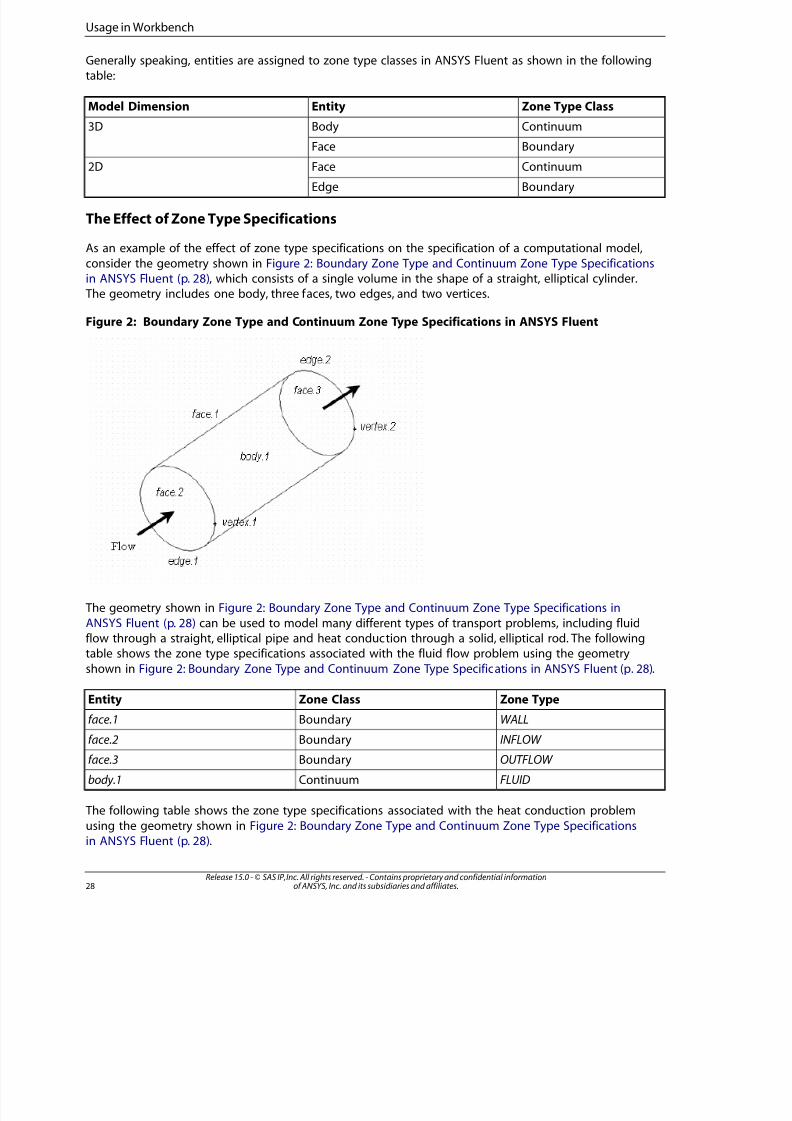
8/10/2019 ANSYS Meshing Users Guide
http://slidepdf.com/reader/full/ansys-meshing-users-guide 36/491
Generally speaking, entities are assigned to zone type classes in ANSYS Fluent as shown in the followingtable:
Zone Type ClassEntityModel Dimension
ContinuumBody3D
BoundaryFace
ContinuumFace2D
BoundaryEdge
The Effect of Zone Type Specifications
As an example of the effect of zone type specifications on the specification of a computational model,
consider the geometry shown in Figure 2: Boundary Zone Type and Continuum Zone Type Specificationsin ANSYS Fluent (p. 28), which consists of a single volume in the shape of a straight, elliptical cylinder. The geometry includes one body, three faces, two edges, and two vertices.
Figure 2: Boundary Zone Type and Continuum Zone Type Specifications in ANSYS Fluent
The geometry shown in Figure 2: Boundary Zone Type and Continuum Zone Type Specifications in
ANSYS Fluent (p. 28) can be used to model many different types of transport problems, including fluidflow through a straight, elliptical pipe and heat conduction through a solid, elliptical rod. The followingtable shows the zone type specifications associated with the fluid flow problem using the geometry
shown in Figure 2: Boundary Zone Type and Continuum Zone Type Specifications in ANSYS Fluent (p. 28).
Zone TypeZone ClassEntityWALLBoundaryface.1
INFLOW Boundaryface.2
OUTFLOW Boundaryface.3
FLUIDContinuumbody.1
The following table shows the zone type specifications associated with the heat conduction problem
using the geometry shown in Figure 2: Boundary Zone Type and Continuum Zone Type Specificationsin ANSYS Fluent (p. 28).
Release 15.0 - © SAS IP, Inc. All rights reserved. - Contains proprietary and confidential informationof ANSYS, Inc. and its subsidiaries and affiliates.28
Usage in Workbench
8/10/2019 ANSYS Meshing Users Guide
http://slidepdf.com/reader/full/ansys-meshing-users-guide 37/491
Zone TypeZone ClassEntity
WALLBoundaryface.1
SOLIDContinuumbody.1
Note
For additional information about boundary (face) zones and continuum (cell) zones in ANSYSFluent, refer to the documentation available under the Help menu within ANSYS Fluent.
Standard Naming Conventions for Naming Named Selections
This section is applicable to boundary zones only.
If you want to override the default boundary zone type assignments by using Named Selections, naming
conventions have been provided for you to follow. Use these conventions when defining Named Selec-tions in either the ANSYS DesignModeler application or the Meshing application. By following thesenaming conventions consistently, you can ensure that ANSYS Fluent boundary zone types will be assignedcorrectly and predictably in the exported ANSYS Fluent file.
When naming Named Selections, it is best practice to specify the appropriate name from the list belowexactly as shown (case-insensitive). In cases where the name shown below contains an underscorecharacter, a hyphen is also acceptable (for example, both EXHAUST_FAN and EXHAUST-FAN will work).(Note, however, that although the Meshing application allows both hyphens and underscore characters
to be used when defining Named Selections, the DesignModeler application allows only underscorecharacters.)
The name of each Named Selection is filtered upon export such that only allowable characters remain.
Allowable characters include all alphanumeric characters as well as the following special characters:
` ! $ % ^ & * _ + - = : < > . ? /
All other characters, including spaces, are invalid. If an invalid character is used, it is replaced by an
underscore (_) upon export.
In addition, the export process does allow for partial matches and special abbreviations, which are de-scribed in Zone Type Assignment (p. 30).
AXIS
EXHAUST_FAN
FAN
INLET_VENT
INTAKE_FAN
INTERFACE INTERIOR
MASS_FLOW_INLET
OUTFLOW
OUTLET_VENT
PERIODIC
POROUS_JUMP
PRESSURE_FAR_FIELD
PRESSURE_INLET
PRESSURE_OUTLET
29Release 15.0 - © SAS IP, Inc. All rights reserved. - Contains proprietary and confidential informationof ANSYS, Inc. and its subsidiaries and affiliates.
Exporting Meshes or Faceted Geometry
8/10/2019 ANSYS Meshing Users Guide
http://slidepdf.com/reader/full/ansys-meshing-users-guide 38/491
RADIATOR
RECIRCULATION_INLET
RECIRCULATION_OUTLET
SYMMETRY
THIN
VELOCITY_INLET
WALL
Note
For details about the boundary (face) zone and continuum (cell) zone types in ANSYS Fluent,refer to the documentation available under the Help menu within ANSYS Fluent.
Zone Type Assignment
This section describes zone naming and the zone type assignment process.
Zone Naming
By default, zones are named after the part and body from which they are derived. For example, part“part” and body “solid body” will result in a zone name of “part-solid_body.” When the zone name iscreated:
• Any invalid characters (such as the space in “solid body”) are replaced by an underscore character(“solid_body”).
• Names that begin with a digit are prefixed by “zone.”
• If the part name and the body name are identical, only the body name is used to create the zonename. The same rule applies to single body parts.
Note
If you set the Auto Zone Type Assignment option to Off (as described in Meshing Options
on the Options Dialog Box (p. 225)), all boundary zones are set to the default zone type WALL.
If a boundary zone was created for a Named Selection (as described in Classes of Zone Types in ANSYSFluent (p. 26)), the name of the boundary zone is set to the name of the Named Selection.
In cases where the zone naming process could lead to conflicting zone names (for example, in a situation
where the potential exists for a zone name that is already in use to be used to name a new zone), oneof the following approaches is used:
• If the zone type is not similar to the zone name in question, the zone type will be prefixed to the
zone name to make it unique. For example, an existing continuum zone named “fluid” and a newboundary zone named “fluid” (with zone type WALL) will result in the boundary zone being renamed“wall-fluid.”
A unique integer will be suffixed to the zone name, preceded by a dot character (.). For example,
an existing continuum zone named “solid” (with zone type SOLID) and another continuum zonenamed “solid” (with zone type FLUID) will result in the continuum zone being renamed “solid.1.”
Release 15.0 - © SAS IP, Inc. All rights reserved. - Contains proprietary and confidential informationof ANSYS, Inc. and its subsidiaries and affiliates.30
Usage in Workbench
8/10/2019 ANSYS Meshing Users Guide
http://slidepdf.com/reader/full/ansys-meshing-users-guide 39/491
• If the zone type is similar to the zone name in question, the approach is dependent on whether thezone is a continuum zone or a boundary zone:
– If multiple continuum zones have the same type and same zone name, they are merged into asingle continuum zone.
– If multiple boundary zones have the same type and same zone name, a unique integer will be
suffixed to the zone name, preceded by a dot character (.). For example, an existing boundary zone
named “wall” and a second boundary zone named “wall” will result in the second boundary zonebeing renamed “wall.1.” Subsequent boundary zones named “wall” will be renamed “wall.2,”“wall.3,”
and so on.
Because part and body names influence the creation of continuum zones in ANSYS Fluent, it is bestpractice to assign distinct part and body names that follow these rules:
• Names should include only allowable characters. Allowable characters include all alphanumeric
characters as well as the following special characters:
` ! $ % ^ & * _ + - = : < > . ? /
All other characters, including spaces, are invalid. If an invalid character is used, it is replaced byan underscore (_) upon export.
• It is not sufficient for part and body names to differ by case only. This approach may lead to nameconflicts for zones in ANSYS Fluent, because names are converted to all lowercase characters upon
export.
• Using "INTER" as zone name or part of a zone name should be avoided. Because the mesher doesnot allow named selections with identical names and interface definitions require two named selectionsusing "INTER" can cause zone type conflicts.
Zone Type Assignment Process
The section is applicable to boundary zones only.
The zone type is derived from the zone name. To assign zone types, the string comparison operationsdetailed below are performed during the export process. These string comparison operations, which
correspond to the naming conventions described in Standard Naming Conventions for Naming NamedSelections (p. 29), are applied in the order in which they are listed below (that is, at first an exact matchis tested, after that a partial match is tested, etc.) and are always case-insensitive. For example, fan, Fan,
FAn, and faN are all exact matches for the 'FAN' string comparison and result in a zone type of FAN
being assigned.
When the search operation begins, it will start by searching the first portion (or sub-string) of the string
and if no match is found, it will search for a match anywhere in the string. For example, if a NamedSelection with the name wall_inlet_flange is defined, it will be exported as zone type WALL. The 'inlet'portion of the name will have no effect on zone type assignment.
In some cases a name may match multiple patterns or rules, and the expected zone type may not be
assigned. For this reason it is strongly advisable to use only unambiguous names that exactly matchone of the rules presented below.
Once they are exported, names are all lowercase. The single quotation marks that are shown enclosingthe strings below are not considered during the string comparison operations.
3Release 15.0 - © SAS IP, Inc. All rights reserved. - Contains proprietary and confidential informationof ANSYS, Inc. and its subsidiaries and affiliates.
Exporting Meshes or Faceted Geometry

8/10/2019 ANSYS Meshing Users Guide
http://slidepdf.com/reader/full/ansys-meshing-users-guide 40/491
1. Exact matches are checked:
'AXIS'
'EXHAUST_FAN'
'FAN'
'INLET_VENT'
'INTAKE_FAN'
'INTERFACE'
'INTERIOR'
'MASS_FLOW_INLET'
'OUTFLOW''OUTLET_VENT'
'PERIODIC'
'POROUS_JUMP'
'PRESSURE_FAR_FIELD'
'PRESSURE_INLET'
'PRESSURE_OUTLET'
'RADIATOR'
'RECIRCULATION_INLET'
'RECIRCULATION_OUTLET'
'SYMMETRY'
'THIN'
'VELOCITY_INLET'
'WALL'
2. Partial matches are considered only if an exact match was not found in step 1:'AXIS'
{'EXHAUST' && 'FAN'}
'FAN'
{'INLET' && 'VENT'}
{'INTAKE' && 'FAN'}
'INTERFACE'
'INTERIOR'
{'MASS' && 'FLOW' && 'INLET'}
'OUTFLOW'
{'OUTLET' && 'VENT'}
'PERIODIC'
{'POROUS' && 'JUMP'}
{'PRESSURE' && 'FAR' && 'FIELD'}
{'PRESSURE' && 'INLET'}
{'PRESSURE' && 'OUTLET'}'RADIATOR'
{'RECIRCULATION' && 'INLET'}
{'RECIRCULATION' && 'OUTLET'}
'SYMMETRY'
{'VELOCITY' && 'INLET'}
3. String comparisons to the special abbreviations listed in the table below are performed if no match wasfound in step 1 or step 2. If an exact match to one of the strings listed in the table is found, the corres-
ponding zone type is assigned:
This zone type is assigned...When a match for this string is found...
INTERFACE 'CNDBY'
EXHAUST FAN 'EXFAN'
INTERFACE 'IFACE'
PRESSURE INLET 'IN'
INTAKE FAN 'INFAN'
INTERFACE 'INTERFACE'
Release 15.0 - © SAS IP, Inc. All rights reserved. - Contains proprietary and confidential informationof ANSYS, Inc. and its subsidiaries and affiliates.32
Usage in Workbench

8/10/2019 ANSYS Meshing Users Guide
http://slidepdf.com/reader/full/ansys-meshing-users-guide 41/491
This zone type is assigned...When a match for this string is found...
INLET VENT 'IVENT'
MASS FLOW INLET 'MASFI'
PRESSURE OUTLET 'OUT'
OUTLET VENT 'OVENT'
PERIODIC 'PER'
PRESSURE FAR FIELD'PFAR'
POROUS JUMP 'PORJ'
PRESSURE FAR FIELD'PRESF'
PRESSURE INLET 'PRESI'
PRESSURE OUTLET 'PRESO'
PRESSURE FAR FIELD'PRESS'
RADIATOR'RAD'
RECIRCULATION INLET 'RINLT'
RECIRCULATION OUTLET 'ROUT'
INTERFACE 'SLIDE'
SYMMETRY 'SYM'
SYMMETRY 'SYMET'
SYMMETRY 'SYMM'
VELOCITY INLET 'VELF'
VELOCITY INLET 'VELI'
4. Partial matches are considered if no match was found in steps 1, 2, or 3. If a partial match to one of thestrings listed in the following table is found, the corresponding zone type is assigned:
This zone type is assigned...When a match for this string is found...
EXHAUST FAN 'EXHAUST'
VELOCITY INLET 'INLET'
PRESSURE OUTLET 'OUTLET'
SYMMETRY 'SYM'
THIN 'THIN'
WALL'WALL'
33Release 15.0 - © SAS IP, Inc. All rights reserved. - Contains proprietary and confidential informationof ANSYS, Inc. and its subsidiaries and affiliates.
Exporting Meshes or Faceted Geometry

8/10/2019 ANSYS Meshing Users Guide
http://slidepdf.com/reader/full/ansys-meshing-users-guide 42/491
5. If none of the string comparisons described in steps 1, 2, 3, or 4 result in a match, the boundary zone isassigned zone type WALL by default.
Note
• If you are using CutCell and are defining Named Selections for 3D bodies, it is best practiceto avoid the use of ANSYS Fluent keywords. For example, do not include the string "inlet" in
the Named Selection name.
• When Named Selections defined in the ANSYS DesignModeler application are required in theMeshing application, you must set the appropriate geometry import options to ensure theNamed Selections will be transferred properly. Refer to Importing DesignModeler Named Selec-tions into the Meshing Application (p. 389) for details.
• For assembly meshing algorithms, the names of parts, bodies, and Named Selections shouldbe limited to 64 characters.
Special Cases
Be aware of the following special cases related to boundary zone type assignment:
• If Physics Preference (p. 65) is set to CFD and no other zone assignment has been explicitly defined,all zones are exported as FLUID zones. See Fluent Mesh Export (p. 24) for more information.
• A boundary zone type of INTERFACE is assigned automatically to the contact source and contact target
entities that compose contact regions at the time of mesh export. For this reason, you are not requiredto explicitly define INTERFACE zones to resolve contact regions. The zone type of INTERFACE , alongwith the contact information, is written to the mesh file.
When reading the mesh file, ANSYS Fluent creates a mesh interface for each contact region
automatically. Each interface can consist of any number of INTERFACE zones for the source andany number of INTERFACE zones for the target.
For 3D meshes, only face zones referenced in the contact region are considered during export.
For 2D meshes, only face zones consisting of edges are considered. Each contact region cancontain one or more face zones as sources and one or more face zones as targets. If any entityreferenced in a contact region (either as source or target) is also contained in a Named Selection,that contact region is not considered during export.
For more accurate results in cases in which one face zone in a pair has a higher element countthan the other, the zone with the lower element count should be defined as Interface Zone 1of the mesh interface and the zone with the higher element count should be defined as Interface
Zone 2. In the transfer of the contact region source and target regions it is ensured that thesource regions are defined as interface zone 1 and the target regions as interface zone 2.
• A boundary zone type of INTERIOR is assigned automatically between two FLUID zones (sharing a
common boundary) at the time of mesh export. For this reason, you are not required to explicitlydefine an INTERIOR zone in such cases if the name of this zone does not contain any special namederived from the part/body or Named Selection name.
Release 15.0 - © SAS IP, Inc. All rights reserved. - Contains proprietary and confidential informationof ANSYS, Inc. and its subsidiaries and affiliates.34
Usage in Workbench

8/10/2019 ANSYS Meshing Users Guide
http://slidepdf.com/reader/full/ansys-meshing-users-guide 43/491
• A boundary zone type of WALL is assigned automatically to a baffle, unless the baffle is part of aNamed Selection that was defined in the ANSYS DesignModeler application or the Meshing application,
and the name of the Named Selection results in a different zone type assignment.
• A boundary zone type of WALL is assigned automatically between a FLUID zone and a SOLID zone atthe time of mesh export. For this reason, you are not required to explicitly define a WALL zone in
such cases. When reading the mesh file, ANSYS Fluent will generate an additional WALL SHADOW
zone automatically.
• Due to a limitation concerning the definition of rotational/translational periodicity in ANSYS Workbench
the boundary zone type PERIODIC is always replaced by the boundary zone type WALL during themesh export process. (However, the zone name is kept.) The suggested workaround is to manuallyredefine periodic boundary conditions in ANSYS Fluent. For details, refer to the documentationavailable under the Help menu within ANSYS Fluent.
Examples of Fluent Mesh Export: An Alternative to Using a Fluid Flow (Fluent) Analysis
System
The first example illustrates the basic workflow you can follow to create a multibody part in the ANSYS
DesignModeler application, mesh the model in the Meshing application, and export the mesh to ANSYSFluent. In the example, the bodies are renamed in the DesignModeler application, and Named Selectionsare defined in the Meshing application. Based on these definitions, ANSYS Fluent zone names/typesare assigned correctly and predictably (for both continuum and boundary zones) in the exported Fluent
mesh file.
First, the model is imported into the DesignModeler application. The model consists of nine solid bodiesafter import. In the DesignModeler application, a multibody part is formed, the bodies are renamed,
and all bodies are assigned a material property of fluid. (See Fluent Mesh Export (p. 24) for more inform-ation about the Fluid/Solid material property in the DesignModeler application.) Shared Topology isalso used in this example. Refer to Figure 3: Multibody Part Containing All Fluid Bodies in the Design-Modeler Application (p. 36).
35Release 15.0 - © SAS IP, Inc. All rights reserved. - Contains proprietary and confidential informationof ANSYS, Inc. and its subsidiaries and affiliates.
Exporting Meshes or Faceted Geometry
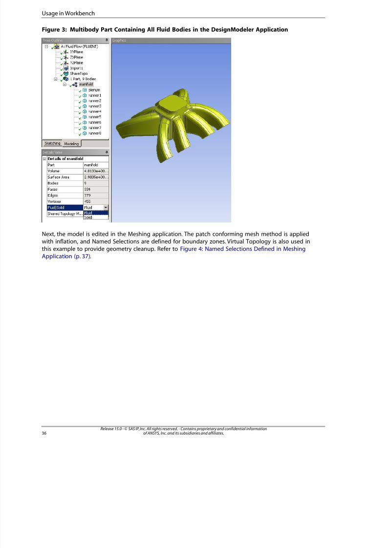
8/10/2019 ANSYS Meshing Users Guide
http://slidepdf.com/reader/full/ansys-meshing-users-guide 44/491
Figure 3: Multibody Part Containing All Fluid Bodies in the DesignModeler Application
Next, the model is edited in the Meshing application. The patch conforming mesh method is appliedwith inflation, and Named Selections are defined for boundary zones. Virtual Topology is also used inthis example to provide geometry cleanup. Refer to Figure 4: Named Selections Defined in Meshing
Application (p. 37).
Release 15.0 - © SAS IP, Inc. All rights reserved. - Contains proprietary and confidential informationof ANSYS, Inc. and its subsidiaries and affiliates.36
Usage in Workbench
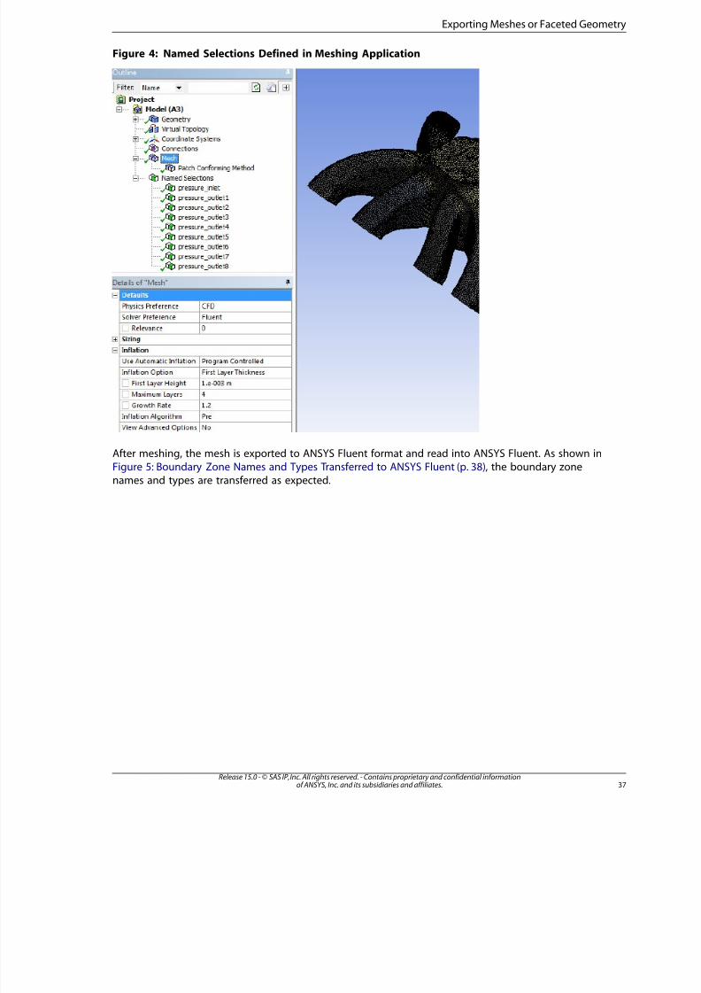
8/10/2019 ANSYS Meshing Users Guide
http://slidepdf.com/reader/full/ansys-meshing-users-guide 45/491
Figure 4: Named Selections Defined in Meshing Application
After meshing, the mesh is exported to ANSYS Fluent format and read into ANSYS Fluent. As shown in
Figure 5: Boundary Zone Names and Types Transferred to ANSYS Fluent (p. 38), the boundary zonenames and types are transferred as expected.
37Release 15.0 - © SAS IP, Inc. All rights reserved. - Contains proprietary and confidential informationof ANSYS, Inc. and its subsidiaries and affiliates.
Exporting Meshes or Faceted Geometry
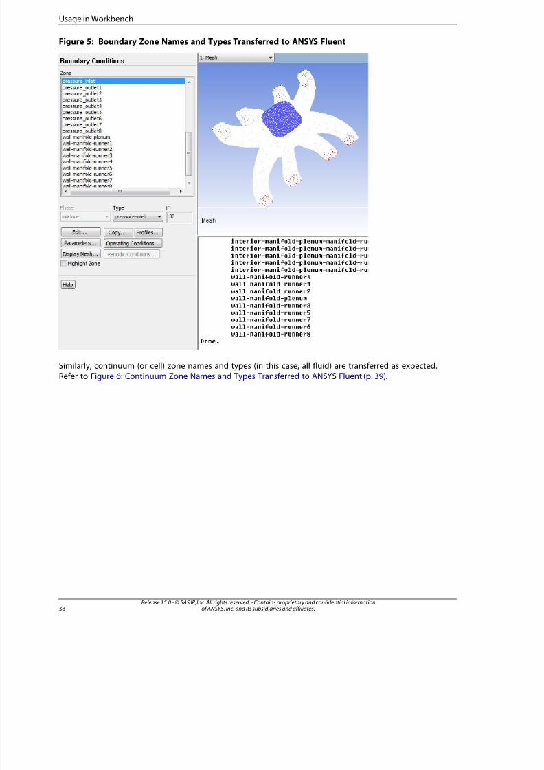
8/10/2019 ANSYS Meshing Users Guide
http://slidepdf.com/reader/full/ansys-meshing-users-guide 46/491
Figure 5: Boundary Zone Names and Types Transferred to ANSYS Fluent
Similarly, continuum (or cell) zone names and types (in this case, all fluid) are transferred as expected.Refer to Figure 6: Continuum Zone Names and Types Transferred to ANSYS Fluent (p. 39).
Release 15.0 - © SAS IP, Inc. All rights reserved. - Contains proprietary and confidential informationof ANSYS, Inc. and its subsidiaries and affiliates.38
Usage in Workbench
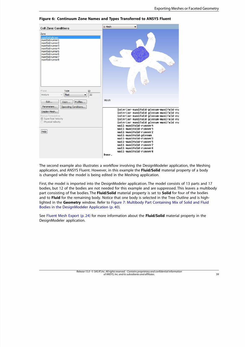
8/10/2019 ANSYS Meshing Users Guide
http://slidepdf.com/reader/full/ansys-meshing-users-guide 47/491
Figure 6: Continuum Zone Names and Types Transferred to ANSYS Fluent
The second example also illustrates a workflow involving the DesignModeler application, the Meshingapplication, and ANSYS Fluent. However, in this example the Fluid/Solid material property of a bodyis changed while the model is being edited in the Meshing application.
First, the model is imported into the DesignModeler application. The model consists of 13 parts and 17bodies, but 12 of the bodies are not needed for this example and are suppressed. This leaves a multibodypart consisting of five bodies. The Fluid/Solid material property is set to Solid for four of the bodiesand to Fluid for the remaining body. Notice that one body is selected in the Tree Outline and is high-
lighted in the Geometry window. Refer to Figure 7: Multibody Part Containing Mix of Solid and FluidBodies in the DesignModeler Application (p. 40).
See Fluent Mesh Export (p. 24) for more information about the Fluid/Solid material property in the
DesignModeler application.
39Release 15.0 - © SAS IP, Inc. All rights reserved. - Contains proprietary and confidential informationof ANSYS, Inc. and its subsidiaries and affiliates.
Exporting Meshes or Faceted Geometry
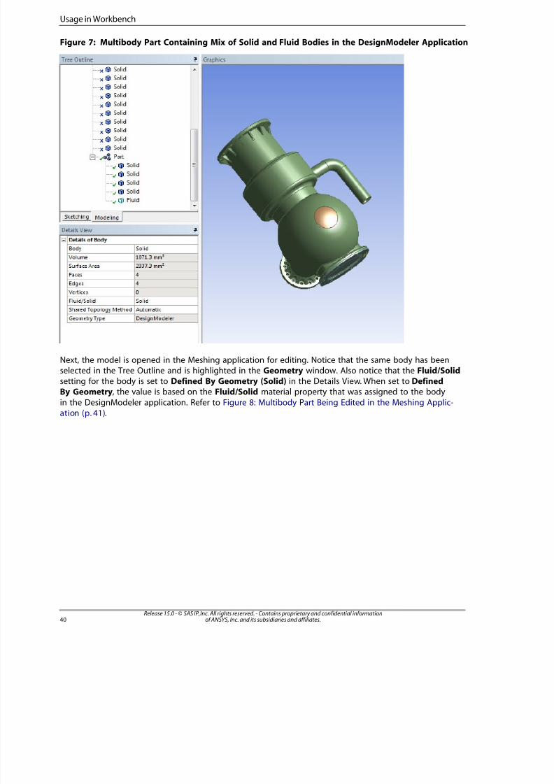
8/10/2019 ANSYS Meshing Users Guide
http://slidepdf.com/reader/full/ansys-meshing-users-guide 48/491
Figure 7: Multibody Part Containing Mix of Solid and Fluid Bodies in the DesignModeler Application
Next, the model is opened in the Meshing application for editing. Notice that the same body has been
selected in the Tree Outline and is highlighted in the Geometry window. Also notice that the Fluid/Solidsetting for the body is set to Defined By Geometry (Solid) in the Details View. When set to DefinedBy Geometry, the value is based on the Fluid/Solid material property that was assigned to the body
in the DesignModeler application. Refer to Figure 8: Multibody Part Being Edited in the Meshing Applic-ation (p. 41).
Release 15.0 - © SAS IP, Inc. All rights reserved. - Contains proprietary and confidential informationof ANSYS, Inc. and its subsidiaries and affiliates.40
Usage in Workbench
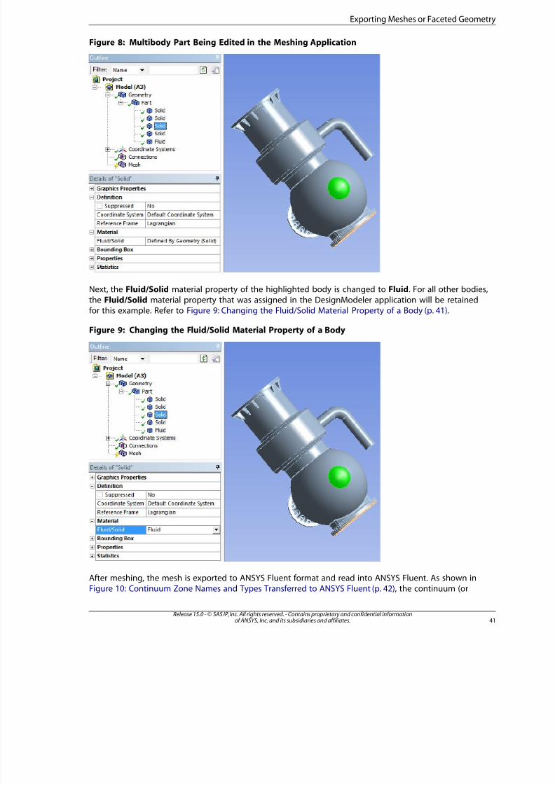
8/10/2019 ANSYS Meshing Users Guide
http://slidepdf.com/reader/full/ansys-meshing-users-guide 49/491
Figure 8: Multibody Part Being Edited in the Meshing Application
Next, the Fluid/Solid material property of the highlighted body is changed to Fluid. For all other bodies,the Fluid/Solid material property that was assigned in the DesignModeler application will be retainedfor this example. Refer to Figure 9: Changing the Fluid/Solid Material Property of a Body (p. 41).
Figure 9: Changing the Fluid/Solid Material Property of a Body
After meshing, the mesh is exported to ANSYS Fluent format and read into ANSYS Fluent. As shown inFigure 10: Continuum Zone Names and Types Transferred to ANSYS Fluent (p. 42), the continuum (or
4Release 15.0 - © SAS IP, Inc. All rights reserved. - Contains proprietary and confidential informationof ANSYS, Inc. and its subsidiaries and affiliates.
Exporting Meshes or Faceted Geometry
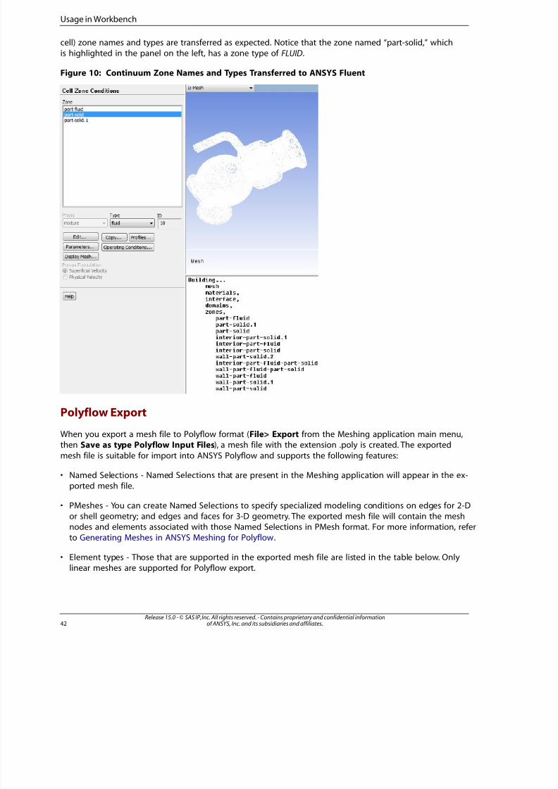
8/10/2019 ANSYS Meshing Users Guide
http://slidepdf.com/reader/full/ansys-meshing-users-guide 50/491
cell) zone names and types are transferred as expected. Notice that the zone named “part-solid,” whichis highlighted in the panel on the left, has a zone type of FLUID.
Figure 10: Continuum Zone Names and Types Transferred to ANSYS Fluent
Polyflow Export
When you export a mesh file to Polyflow format (File> Export from the Meshing application main menu,then Save as type Polyflow Input Files), a mesh file with the extension .poly is created. The exported
mesh file is suitable for import into ANSYS Polyflow and supports the following features:
• Named Selections - Named Selections that are present in the Meshing application will appear in the ex-ported mesh file.
• PMeshes - You can create Named Selections to specify specialized modeling conditions on edges for 2-Dor shell geometry; and edges and faces for 3-D geometry. The exported mesh file will contain the meshnodes and elements associated with those Named Selections in PMesh format. For more information, referto Generating Meshes in ANSYS Meshing for Polyflow.
• Element types - Those that are supported in the exported mesh file are listed in the table below. Onlylinear meshes are supported for Polyflow export.
Release 15.0 - © SAS IP, Inc. All rights reserved. - Contains proprietary and confidential informationof ANSYS, Inc. and its subsidiaries and affiliates.42
Usage in Workbench
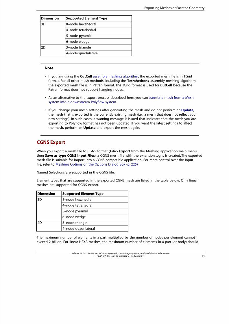
8/10/2019 ANSYS Meshing Users Guide
http://slidepdf.com/reader/full/ansys-meshing-users-guide 51/491
Supported Element TypeDimension
8–node hexahedral3D
4–node tetrahedral
5–node pyramid
6–node wedge
3–node triangle2D
4–node quadrilateral
Note
• If you are using the CutCell assembly meshing algorithm, the exported mesh file is in TGridformat. For all other mesh methods, including the Tetrahedrons assembly meshing algorithm,
the exported mesh file is in Patran format. The TGrid format is used for CutCell because thePatran format does not support hanging nodes.
• As an alternative to the export process described here, you can transfer a mesh from a Mesh
system into a downstream Polyflow system.
• If you change your mesh settings after generating the mesh and do not perform an Update,the mesh that is exported is the currently existing mesh (i.e., a mesh that does not reflect yournew settings). In such cases, a warning message is issued that indicates that the mesh you are
exporting to Polyflow format has not been updated. If you want the latest settings to affectthe mesh, perform an Update and export the mesh again.
CGNS Export
When you export a mesh file to CGNS format (File> Export from the Meshing application main menu,then Save as type CGNS Input Files), a CGNS mesh file with the extension .cgns is created. The exportedmesh file is suitable for import into a CGNS-compatible application. For more control over the input
file, refer to Meshing Options on the Options Dialog Box (p. 225).
Named Selections are supported in the CGNS file.
Element types that are supported in the exported CGNS mesh are listed in the table below. Only linear
meshes are supported for CGNS export.
Supported Element TypeDimension
8–node hexahedral3D
4–node tetrahedral
5–node pyramid
6–node wedge
3–node triangle2D
4–node quadrilateral
The maximum number of elements in a part multiplied by the number of nodes per element cannotexceed 2 billion. For linear HEXA meshes, the maximum number of elements in a part (or body) should
43Release 15.0 - © SAS IP, Inc. All rights reserved. - Contains proprietary and confidential informationof ANSYS, Inc. and its subsidiaries and affiliates.
Exporting Meshes or Faceted Geometry

8/10/2019 ANSYS Meshing Users Guide
http://slidepdf.com/reader/full/ansys-meshing-users-guide 52/491
not exceed 250 million elements. For linear TETRA meshes, the maximum number of elements in a part(or body) should not exceed 500 million elements.
To export larger meshes, split them into several smaller parts (or Named Selections).
If you exceed the CGNS export limits, you will get the error message:
Error: CGNS section CGNS_section_name exceeds maximum mesh size limit, please split the mesh into smaller sect
ANSYS ICEM CFD Export
When you export from the Meshing application to ANSYS ICEM CFD format, an ANSYS ICEM CFD projectfile with the extension .prj, along with a geometry file (*.tin) and/or mesh file (*.uns) are written. Thefiles that are created are the same as those that are created if you begin in ANSYS ICEM CFD and use
its Workbench Readers option to import a file from the Meshing application.
Anytime you plan to export from the Meshing application to ANSYS ICEM CFD format, it is best practiceto define the desired part and body names for your model in the DesignModeler application prior to
meshing the model in the Meshing application. This is recommended because the ANSYS ICEM CFDpart names will be derived from the part and body names that are defined for the model when you
initially open the model in the Meshing application; the export process will ignore any renaming orNamed Selections created in the Meshing application.
There are three ways to export meshing data to ICEM CFD format:
1. Choose File> Export from the Meshing application main menu, then Save as type ICEM CFD InputFiles.
ANSYS ICEM CFD part names that appear in the exported files are derived from the ANSYSWorkbench geometry part and body names. In the case of a single body part, only the bodyname is used.
Note
The concept of a part in ANSYS Workbench and a part in ANSYS ICEM CFD isnot the same. For information about parts in ANSYS Workbench, refer to Con-formal Meshing Between Parts (p. 5) in the Meshing application help andGeometry Basics in the Mechanical help. For information about parts in ANSYS
ICEM CFD, refer to the documentation available under the Help menu withinANSYS ICEM CFD.
2. Save your ANSYS Workbench files (*.mechdat or *.meshdat) and use the ANSYS ICEM CFD File >Workbench Readers option to import the files into ANSYS ICEM CFD (as long as ANSYS Workbench
and ANSYS ICEM CFD are installed on the same machine). Legacy formats such as *.dsdb and *.cmdbare also supported.
Any defined Named Selections will be imported into ANSYS ICEM CFD as subsets because
subsets support non-exclusive sets (overlapping Named Selections). However, each entity canonly be in a single part (exclusive sets). In cases where you want overlapping Named Selectionsto be converted to ANSYS ICEM CFD parts, the overlapping subsets can be cleaned up in ANSYSICEM CFD and then converted into parts. For details about handling imported ANSYS Workbench
files in ANSYS ICEM CFD, refer to the documentation available under the Help menu withinANSYS ICEM CFD.
Release 15.0 - © SAS IP, Inc. All rights reserved. - Contains proprietary and confidential informationof ANSYS, Inc. and its subsidiaries and affiliates.44
Usage in Workbench

8/10/2019 ANSYS Meshing Users Guide
http://slidepdf.com/reader/full/ansys-meshing-users-guide 53/491
3. Use the ANSYS ICEM CFD Workbench Add-In. In ANSYS Workbench, right-click on a Geometry orMesh cell and choose Transfer Data Into New > ICEM CFD. The advantage of the Add-In connection
is that it maintains the connectivity once the geometry is modified so, unlike the previous twomethods, you can easily refresh the geometry in ICEM CFD and then update the mesh and thesolver input. For more information, see Component Systems in the [ANSYS Workbench User's Guide].
Rules Followed By the Export Process
When exporting to ANSYS ICEM CFD format, these rules are followed:
Note
The series of examples that follows this list illustrates many of the rules listed here.
• To achieve unique ANSYS ICEM CFD part names in the ANSYS ICEM CFD format files, a unique integeris suffixed to all ANSYS Workbench part/body names.
• A single body part in ANSYS Workbench will appear as < part_name>_< part_index > in the ANSYSICEM CFD format files.
• A multibody part in ANSYS Workbench will appear as < part_name>_< part_in-
dex >/<body_name>_<body_index > in the ANSYS ICEM CFD format files. The / character denoteshierarchy.
• Bodies that are in a multibody part in ANSYS Workbench are put into an ANSYS ICEM CFD assembly. The structuring in the ANSYS ICEM CFD format files reflects the part/body structure present in ANSYS
Workbench.
• As long as they are not contained in Named Selections, faces that are shared between bodies in thesame multibody part in ANSYS Workbench are put into separate ANSYS ICEM CFD parts. This type of
shared face is named according to the bodies having the face in common, with the body names
separated by the # character.
• Entities that are contained in a Named Selection are put into a separate ANSYS ICEM CFD part.
• For each body, an ANSYS ICEM CFD Material Point is created and put into the corresponding ANSYSICEM CFD part. The names of Material Points have the suffix _MATPOINT.
• If a mesh has been generated, it is exported along with the geometry. In such cases, these additionalrules are followed:
– As long as they are not contained in a Named Selection, node/line/surface mesh cells are associatedwith the corresponding geometry part/body in ANSYS ICEM CFD.
– As long as they are not contained in a Named Selection, volume mesh cells are associated with
the Material Point part.
– Mesh cells that are associated with geometry entities that are contained in a Named Selection areassociated with the ANSYS ICEM CFD part that corresponds to that Named Selection.
The first example is a model consisting of four separate single body parts in ANSYS Workbench. Thesingle body parts are named fluid1, fluid2, fluid3, and fluid4. The table below shows the geometry inANSYS Workbench and the corresponding part names that will appear in ANSYS ICEM CFD:
45Release 15.0 - © SAS IP, Inc. All rights reserved. - Contains proprietary and confidential informationof ANSYS, Inc. and its subsidiaries and affiliates.
Exporting Meshes or Faceted Geometry
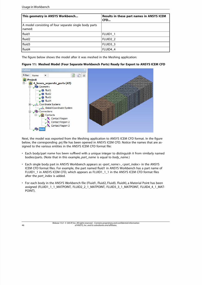
8/10/2019 ANSYS Meshing Users Guide
http://slidepdf.com/reader/full/ansys-meshing-users-guide 54/491
Results in these part names in ANSYS ICEMCFD...
This geometry in ANSYS Workbench...
A model consisting of four separate single body parts
named:
FLUID1_1fluid1
FLUID2_2fluid2
FLUID3_3fluid3FLUID4_4fluid4
The figure below shows the model after it was meshed in the Meshing application:
Figure 11: Meshed Model (Four Separate Workbench Parts) Ready for Export to ANSYS ICEM CFD
Next, the model was exported from the Meshing application to ANSYS ICEM CFD format. In the figurebelow, the corresponding .prj file has been opened in ANSYS ICEM CFD. Notice the names that are as-signed to the various entities in the ANSYS ICEM CFD format file:
• Each body/part name has been suffixed with a unique integer to distinguish it from similarly namedbodies/parts. (Note that in this example, part_name is equal to body_name.)
• Each single body part in ANSYS Workbench appears as < part_name>_< part_index > in the ANSYS
ICEM CFD format files. For example, the part named fluid1 in ANSYS Workbench has a part name of FLUID1_1 in ANSYS ICEM CFD, which appears as FLUID1_1_1 in the ANSYS ICEM CFD format filesafter the part_index is added.
• For each body in the ANSYS Workbench file (Fluid1, Fluid2, Fluid3, Fluid4), a Material Point has been
assigned (FLUID1_1_1_MATPOINT, FLUID2_2_1_MATPOINT, FLUID3_3_1_MATPOINT, FLUID4_4_1_MAT-POINT).
Release 15.0 - © SAS IP, Inc. All rights reserved. - Contains proprietary and confidential informationof ANSYS, Inc. and its subsidiaries and affiliates.46
Usage in Workbench
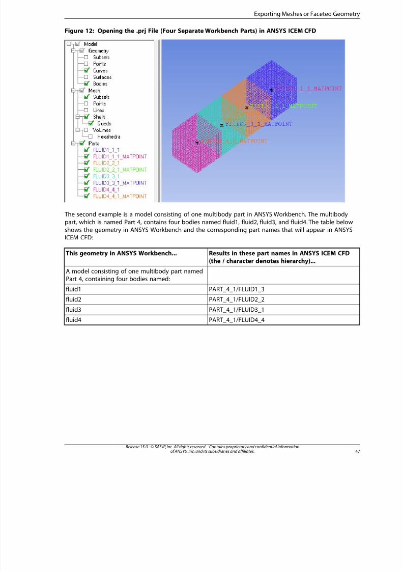
8/10/2019 ANSYS Meshing Users Guide
http://slidepdf.com/reader/full/ansys-meshing-users-guide 55/491
Figure 12: Opening the .prj File (Four Separate Workbench Parts) in ANSYS ICEM CFD
The second example is a model consisting of one multibody part in ANSYS Workbench. The multibody
part, which is named Part 4, contains four bodies named fluid1, fluid2, fluid3, and fluid4. The table belowshows the geometry in ANSYS Workbench and the corresponding part names that will appear in ANSYSICEM CFD:
Results in these part names in ANSYS ICEM CFD(the / character denotes hierarchy)...
This geometry in ANSYS Workbench...
A model consisting of one multibody part namedPart 4, containing four bodies named:
PART_4_1/FLUID1_3fluid1
PART_4_1/FLUID2_2fluid2
PART_4_1/FLUID3_1fluid3
PART_4_1/FLUID4_4fluid4
47Release 15.0 - © SAS IP, Inc. All rights reserved. - Contains proprietary and confidential informationof ANSYS, Inc. and its subsidiaries and affiliates.
Exporting Meshes or Faceted Geometry
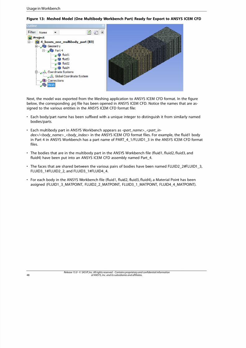
8/10/2019 ANSYS Meshing Users Guide
http://slidepdf.com/reader/full/ansys-meshing-users-guide 56/491
Figure 13: Meshed Model (One Multibody Workbench Part) Ready for Export to ANSYS ICEM CFD
Next, the model was exported from the Meshing application to ANSYS ICEM CFD format. In the figurebelow, the corresponding .prj file has been opened in ANSYS ICEM CFD. Notice the names that are as-
signed to the various entities in the ANSYS ICEM CFD format file:
• Each body/part name has been suffixed with a unique integer to distinguish it from similarly namedbodies/parts.
• Each multibody part in ANSYS Workbench appears as < part_name>_< part_in-
dex >/<body_name>_<body_index > in the ANSYS ICEM CFD format files. For example, the fluid1 body
in Part 4 in ANSYS Workbench has a part name of PART_4_1/FLUID1_3 in the ANSYS ICEM CFD formatfiles.
• The bodies that are in the multibody part in the ANSYS Workbench file (fluid1, fluid2, fluid3, and
fluid4) have been put into an ANSYS ICEM CFD assembly named Part_4.
• The faces that are shared between the various pairs of bodies have been named FLUID2_2#FLUID1_3,FLUID3_1#FLUID2_2, and FLUID3_1#FLUID4_4.
• For each body in the ANSYS Workbench file (fluid1, fluid2, fluid3, fluid4), a Material Point has beenassigned (FLUID1_3_MATPOINT, FLUID2_2_MATPOINT, FLUID3_1_MATPOINT, FLUID4_4_MATPOINT).
Release 15.0 - © SAS IP, Inc. All rights reserved. - Contains proprietary and confidential informationof ANSYS, Inc. and its subsidiaries and affiliates.48
Usage in Workbench
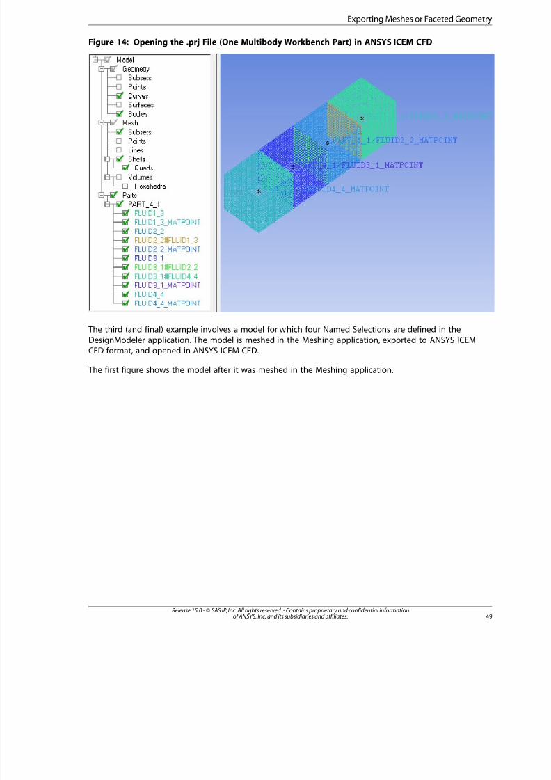
8/10/2019 ANSYS Meshing Users Guide
http://slidepdf.com/reader/full/ansys-meshing-users-guide 57/491
Figure 14: Opening the .prj File (One Multibody Workbench Part) in ANSYS ICEM CFD
The third (and final) example involves a model for which four Named Selections are defined in the
DesignModeler application. The model is meshed in the Meshing application, exported to ANSYS ICEMCFD format, and opened in ANSYS ICEM CFD.
The first figure shows the model after it was meshed in the Meshing application.
49Release 15.0 - © SAS IP, Inc. All rights reserved. - Contains proprietary and confidential informationof ANSYS, Inc. and its subsidiaries and affiliates.
Exporting Meshes or Faceted Geometry
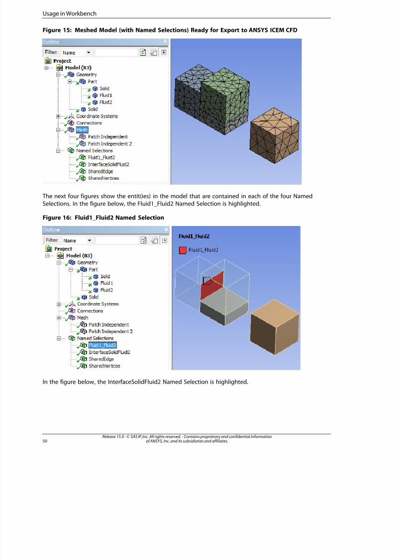
8/10/2019 ANSYS Meshing Users Guide
http://slidepdf.com/reader/full/ansys-meshing-users-guide 58/491
Figure 15: Meshed Model (with Named Selections) Ready for Export to ANSYS ICEM CFD
The next four figures show the entit(ies) in the model that are contained in each of the four NamedSelections. In the figure below, the Fluid1_Fluid2 Named Selection is highlighted.
Figure 16: Fluid1_Fluid2 Named Selection
In the figure below, the InterfaceSolidFluid2 Named Selection is highlighted.
Release 15.0 - © SAS IP, Inc. All rights reserved. - Contains proprietary and confidential informationof ANSYS, Inc. and its subsidiaries and affiliates.50
Usage in Workbench
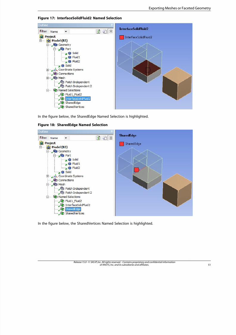
8/10/2019 ANSYS Meshing Users Guide
http://slidepdf.com/reader/full/ansys-meshing-users-guide 59/491
Figure 17: InterfaceSolidFluid2 Named Selection
In the figure below, the SharedEdge Named Selection is highlighted.
Figure 18: SharedEdge Named Selection
In the figure below, the SharedVertices Named Selection is highlighted.
5Release 15.0 - © SAS IP, Inc. All rights reserved. - Contains proprietary and confidential informationof ANSYS, Inc. and its subsidiaries and affiliates.
Exporting Meshes or Faceted Geometry
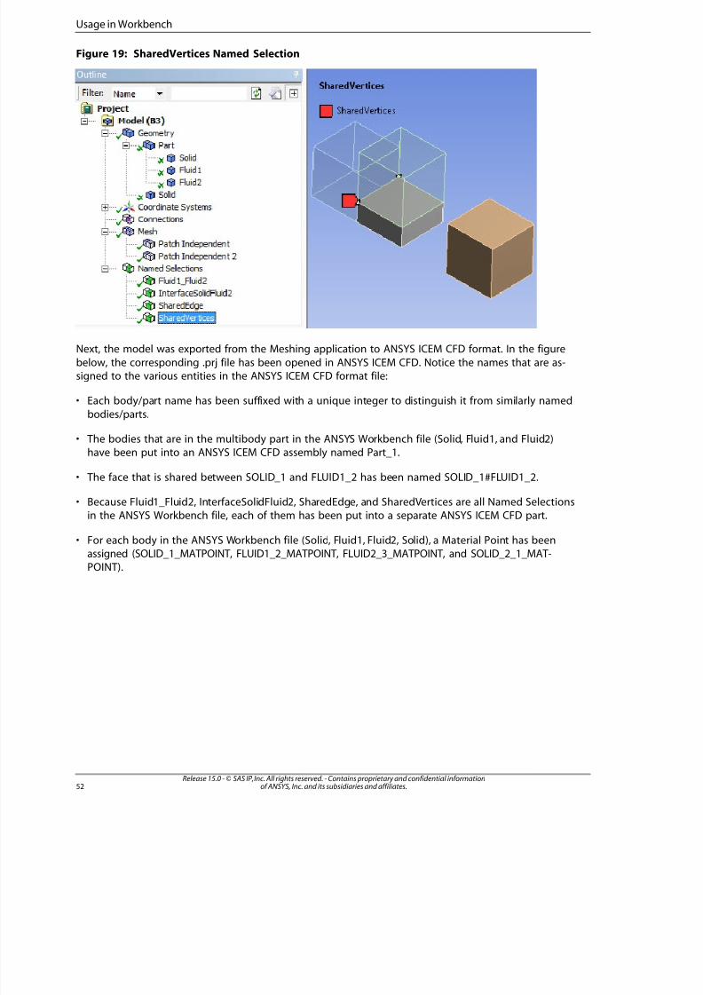
8/10/2019 ANSYS Meshing Users Guide
http://slidepdf.com/reader/full/ansys-meshing-users-guide 60/491
Figure 19: SharedVertices Named Selection
Next, the model was exported from the Meshing application to ANSYS ICEM CFD format. In the figure
below, the corresponding .prj file has been opened in ANSYS ICEM CFD. Notice the names that are as-signed to the various entities in the ANSYS ICEM CFD format file:
• Each body/part name has been suffixed with a unique integer to distinguish it from similarly named
bodies/parts.
• The bodies that are in the multibody part in the ANSYS Workbench file (Solid, Fluid1, and Fluid2)have been put into an ANSYS ICEM CFD assembly named Part_1.
• The face that is shared between SOLID_1 and FLUID1_2 has been named SOLID_1#FLUID1_2.
• Because Fluid1_Fluid2, InterfaceSolidFluid2, SharedEdge, and SharedVertices are all Named Selectionsin the ANSYS Workbench file, each of them has been put into a separate ANSYS ICEM CFD part.
• For each body in the ANSYS Workbench file (Solid, Fluid1, Fluid2, Solid), a Material Point has beenassigned (SOLID_1_MATPOINT, FLUID1_2_MATPOINT, FLUID2_3_MATPOINT, and SOLID_2_1_MAT-POINT).
Release 15.0 - © SAS IP, Inc. All rights reserved. - Contains proprietary and confidential informationof ANSYS, Inc. and its subsidiaries and affiliates.52
Usage in Workbench
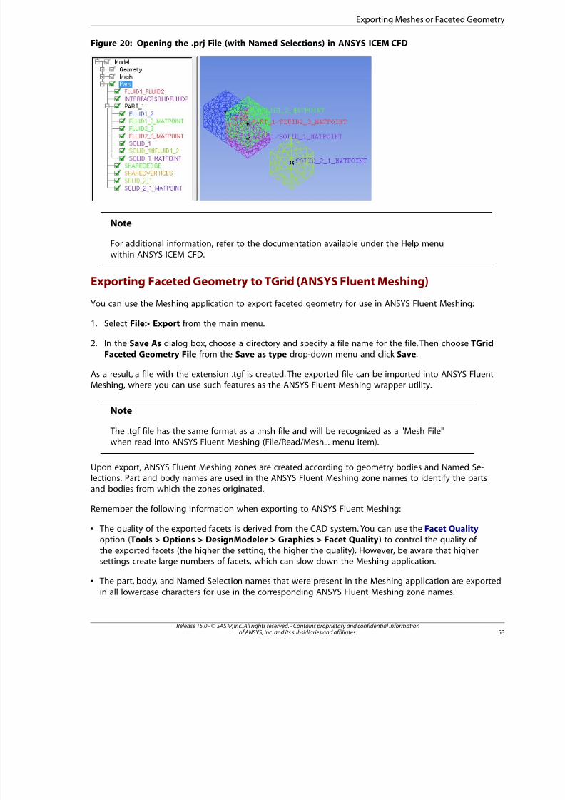
8/10/2019 ANSYS Meshing Users Guide
http://slidepdf.com/reader/full/ansys-meshing-users-guide 61/491
Figure 20: Opening the .prj File (with Named Selections) in ANSYS ICEM CFD
Note
For additional information, refer to the documentation available under the Help menu
within ANSYS ICEM CFD.
Exporting Faceted Geometry to TGrid (ANSYS Fluent Meshing)
You can use the Meshing application to export faceted geometry for use in ANSYS Fluent Meshing:
1. Select File> Export from the main menu.
2. In the Save As dialog box, choose a directory and specify a file name for the file. Then choose TGrid
Faceted Geometry File from the Save as type drop-down menu and click Save.
As a result, a file with the extension .tgf is created. The exported file can be imported into ANSYS FluentMeshing, where you can use such features as the ANSYS Fluent Meshing wrapper utility.
Note
The .tgf file has the same format as a .msh file and will be recognized as a "Mesh File"
when read into ANSYS Fluent Meshing (File/Read/Mesh... menu item).
Upon export, ANSYS Fluent Meshing zones are created according to geometry bodies and Named Se-lections. Part and body names are used in the ANSYS Fluent Meshing zone names to identify the partsand bodies from which the zones originated.
Remember the following information when exporting to ANSYS Fluent Meshing:
• The quality of the exported facets is derived from the CAD system. You can use the Facet Qualityoption (Tools > Options > DesignModeler > Graphics > Facet Quality ) to control the quality of
the exported facets (the higher the setting, the higher the quality). However, be aware that highersettings create large numbers of facets, which can slow down the Meshing application.
• The part, body, and Named Selection names that were present in the Meshing application are exported
in all lowercase characters for use in the corresponding ANSYS Fluent Meshing zone names.
53Release 15.0 - © SAS IP, Inc. All rights reserved. - Contains proprietary and confidential informationof ANSYS, Inc. and its subsidiaries and affiliates.
Exporting Meshes or Faceted Geometry
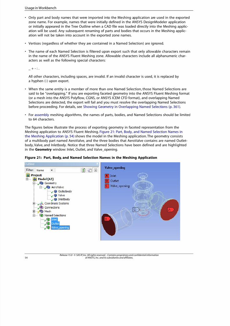
8/10/2019 ANSYS Meshing Users Guide
http://slidepdf.com/reader/full/ansys-meshing-users-guide 62/491
• Only part and body names that were imported into the Meshing application are used in the exportedzone name. For example, names that were initially defined in the ANSYS DesignModeler application
or initially appeared in the Tree Outline when a CAD file was loaded directly into the Meshing applic-ation will be used. Any subsequent renaming of parts and bodies that occurs in the Meshing applic-ation will not be taken into account in the exported zone names.
• Vertices (regardless of whether they are contained in a Named Selection) are ignored.
• The name of each Named Selection is filtered upon export such that only allowable characters remainin the name of the ANSYS Fluent Meshing zone. Allowable characters include all alphanumeric char-
acters as well as the following special characters:
_ + - : .
All other characters, including spaces, are invalid. If an invalid character is used, it is replaced bya hyphen (-) upon export.
• When the same entity is a member of more than one Named Selection, those Named Selections aresaid to be “overlapping.” If you are exporting faceted geometry into the ANSYS Fluent Meshing format(or a mesh into the ANSYS Polyflow, CGNS, or ANSYS ICEM CFD format), and overlapping Named
Selections are detected, the export will fail and you must resolve the overlapping Named Selectionsbefore proceeding. For details, see Showing Geometry in Overlapping Named Selections (p. 361).
• For assembly meshing algorithms, the names of parts, bodies, and Named Selections should be limited
to 64 characters.
The figures below illustrate the process of exporting geometry in faceted representation from theMeshing application to ANSYS Fluent Meshing. Figure 21: Part, Body, and Named Selection Names inthe Meshing Application (p. 54) shows the model in the Meshing application. The geometry consists
of a multibody part named AeroValve, and the three bodies that AeroValve contains are named Outlet-body, Valve, and Inletbody. Notice that three Named Selections have been defined and are highlightedin the Geometry window: Inlet, Outlet, and Valve_opening.
Figure 21: Part, Body, and Named Selection Names in the Meshing Application
Release 15.0 - © SAS IP, Inc. All rights reserved. - Contains proprietary and confidential informationof ANSYS, Inc. and its subsidiaries and affiliates.54
Usage in Workbench
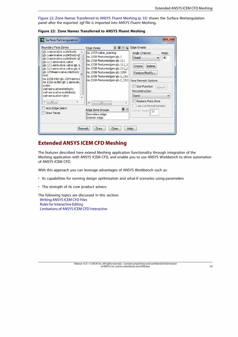
8/10/2019 ANSYS Meshing Users Guide
http://slidepdf.com/reader/full/ansys-meshing-users-guide 63/491
Figure 22: Zone Names Transferred to ANSYS Fluent Meshing (p. 55) shows the Surface Retriangulationpanel after the exported .tgf file is imported into ANSYS Fluent Meshing.
Figure 22: Zone Names Transferred to ANSYS Fluent Meshing
Extended ANSYS ICEM CFD Meshing
The features described here extend Meshing application functionality through integration of the
Meshing application with ANSYS ICEM CFD, and enable you to use ANSYS Workbench to drive automationof ANSYS ICEM CFD.
With this approach you can leverage advantages of ANSYS Workbench such as:
• Its capabilities for running design optimization and what-if scenarios using parameters
• The strength of its core product solvers
The following topics are discussed in this section:Writing ANSYS ICEM CFD FilesRules for Interactive EditingLimitations of ANSYS ICEM CFD Interactive
55Release 15.0 - © SAS IP, Inc. All rights reserved. - Contains proprietary and confidential informationof ANSYS, Inc. and its subsidiaries and affiliates.
Extended ANSYS ICEM CFD Meshing

8/10/2019 ANSYS Meshing Users Guide
http://slidepdf.com/reader/full/ansys-meshing-users-guide 64/491
Writing ANSYS ICEM CFD Files
The Write ICEM CFD Files control determines whether ANSYS ICEM CFD files are written, and includesoptions for running ANSYS ICEM CFD interactively or in batch mode from an ANSYS ICEM CFD Replayfile.
Note
The Write ICEM CFD Files control is available when you use any ANSYS ICEM CFD meshmethod that is available in the Meshing application (Patch Independent Tetra, MultiZone, orMultiZone Quad/Tri). However, the Interactive and Batch options are available only if ANSYS
ICEM CFD is installed. A warning is issued if you try to use one of these options and ANSYSICEM CFD cannot be found.
Note
Another method for writing meshing data to ICEM CFD files is to select the Mesh cell inWorkbench and select Transfer Data to New>ICEM CFD. While the Write ICEM CFD control
writes the geometry of a part, using the ANSYS ICEM CFD Add-in component links to theentire Geometry assembly. For more information, see Component Systems in the ANSYSWorkbench User's Guide.
Options for Write ICEM CFD Files include:
No
No files are written. This is the default.
Yes
Writes ANSYS ICEM CFD files. Useful when you are working in ANSYS Workbench but you want to exportyour project files for further mesh editing in ANSYS ICEM CFD. If this control is set to Yes, your ANSYSICEM CFD project (.prj), geometry (.tin), unstructured domain (.uns), and blocking (.blk) files will be saved
during mesh generation.
• If your ANSYS Workbench project file has been saved, your ANSYS ICEM CFD files will be written to the ANSYSWorkbench project directory. ANSYS Workbench creates a project folder as the top level folder for eachproject, at the same level as the project file. The project folder will be named <filename>_files,
where <filename> is a name you provide. The project file will be named <filename>.wbpj. Under
the project folder is a design point subdirectory for each design point in the project. The active design
point is always design point 0 (dp0) and corresponds to the design point labeled Current in the ANSYS
Workbench GUI. Under each design point folder are system folders for each system type in the project(i.e., Mechanical, Fluent, etc.). Each system folder contains solver-specific files and folders, such as inputfiles, model directories, engineering data, resources, etc. Following this structure, the ANSYS ICEM CFD
files will be written to <filename>_files\dp0\global\MECH\SYS.
Release 15.0 - © SAS IP, Inc. All rights reserved. - Contains proprietary and confidential informationof ANSYS, Inc. and its subsidiaries and affiliates.56
Usage in Workbench
8/10/2019 ANSYS Meshing Users Guide
http://slidepdf.com/reader/full/ansys-meshing-users-guide 65/491
• If your ANSYS Workbench project file has not been saved, your ANSYS ICEM CFD files will be written to thetemporary ANSYS Workbench folder, as follows: %TEMP%\WB_<computer >\unsaved_pro-
ject_files\dp0\global\MECH\SYS.
Note
• Only appropriate files are written, based on the selected mesh method.
• Refer to the ANSYS Workbench help for more information about project file management inANSYS Workbench.
Interactive
Applicable only when ANSYS ICEM CFD is installed.
When the Interactive option is set and you select Generate Mesh, the Meshing application launches
ANSYS ICEM CFD in interactive mode. When you specify the Interactive option, you must also selectan option for ICEM CFD Behavior to determine whether the geometry and/or mesh is transferred to
ANSYS ICEM CFD.
Typically you will run in interactive mode to set up an ANSYS ICEM CFD Replay script file (*.rpl) thatcan be run later in either batch or interactive mode. You will begin by loading a generic Replay file. Itis important to use this default Replay file because the batch process requires the pre and post stepsthat are defined within it. To load the default Replay file:
1. From within ANSYS ICEM CFD, select File > Replay Scripts > Replay Control and the Replay Controlwindow appears.
2. Click Load on the Replay Control window and the Open Script File window appears.
3. Click Open on the Open Script File window to load the default Replay file.
You can incorporate your custom commands into the Replay file by using the Replay Control featureor a text editor. The Replay file will be associated with your ANSYS ICEM CFD project when you save
the project and exit ANSYS ICEM CFD.
After the mesh is returned to the Meshing application and the ANSYS Workbench project is saved, theReplay file will be written to the ANSYS Workbench project directory. Later you can set Write ICEMCFD Files to Batch and the mesh will be updated automatically in batch. You can change parameters
on the ANSYS Workbench project page and Update the mesh in batch from either the project page orfrom within the Meshing application.
Refer to Rules for Interactive Editing (p. 58) and Limitations of ANSYS ICEM CFD Interactive (p. 58) forrelated information.
For more information about Replay Control, refer to the documentation available under the Help menuwithin ANSYS ICEM CFD.
Batch
Applicable only when ANSYS ICEM CFD is installed.
57Release 15.0 - © SAS IP, Inc. All rights reserved. - Contains proprietary and confidential informationof ANSYS, Inc. and its subsidiaries and affiliates.
Extended ANSYS ICEM CFD Meshing

8/10/2019 ANSYS Meshing Users Guide
http://slidepdf.com/reader/full/ansys-meshing-users-guide 66/491
Runs ANSYS ICEM CFD in batch mode from an existing Replay file. If you specify the Batch option, youmust also select an option for ICEM CFD Behavior to determine whether the geometry and/or mesh
is transferred to ANSYS ICEM CFD.
ICEM CFD Behavior
Determines ANSYS ICEM CFD behavior when running ANSYS ICEM CFD in Interactive or Batch mode:
• Post Operation - After the meshing operation completes, transfers both the geometry and mesh toANSYS ICEM CFD for editing.
• Override - Bypasses the meshing operation and transfers only the geometry to ANSYS ICEM CFD formeshing and editing.
Rules for Interactive Editing
The final mesh must pass ANSYS Workbench shape and topology checks in order for the mesh to bereturned to ANSYS Workbench. This requirement imposes the following rules and guidelines for editing
in ANSYS ICEM CFD:
• Do not modify the geometry.
• Pay attention to face and volume part naming. Use the same naming conventions and do not adjust
the part naming.
• Pay attention to mesh quality. If the mesh quality becomes degraded, the mesh will not be returnedto ANSYS Workbench unless the Shape Checking (p. 104) control is set to None.
• Pay attention to mesh projections and associations. It is recommended that you do not change these;however, with some practice changing them may be acceptable.
• Follow file naming conventions for proper archiving and batch interaction. Retain the default names.
Changing the names will break the association between the Replay file and the ANSYS Workbenchproject.
Limitations of ANSYS ICEM CFD Interactive
Be aware of the following limitations when using ANSYS ICEM CFD Interactive:
• ANSYS ICEM CFD Interactive is designed to work at the part level. If you have assigned multiple ANSYSICEM CFD mesh methods (Patch Independent Tetra, MultiZone, or MultiZone Quad/Tri) to different
bodies of a multibody part, the ANSYS ICEM CFD Interactive options specified for the ANSYS ICEMCFD method control that appears lowest in the Tree will be honored. In other words, those ANSYSICEM CFD Interactive options will affect all bodies being meshed with ANSYS ICEM CFD methods re-
gardless of whether a particular option is turned on for a particular body.
• Named Selections are not supported.
Working with Meshing Application Parameters
The term parameters in the Meshing application includes mesh input parameters (such as element size,height of the initial inflation layer, and growth rate) as well as mesh output parameters (number of elements, number of nodes, and mesh metric values).
Release 15.0 - © SAS IP, Inc. All rights reserved. - Contains proprietary and confidential informationof ANSYS, Inc. and its subsidiaries and affiliates.58
Usage in Workbench
8/10/2019 ANSYS Meshing Users Guide
http://slidepdf.com/reader/full/ansys-meshing-users-guide 67/491
A check box appears to the left of each field in the Details View that can be treated as a parameter.Clicking the check box causes a P to appear in the box, which indicates that the field has been exposed
as a parameter for use in the Parameter Workspace. Fields that cannot be parameterized do not containa check box and are left-aligned to save space. The Parameter Workspace collects all specified parametersand lists them in the Parameter Workspace grids for later use and/or modification.
Note
• If an object has a parameterized field, and that object definition is changed in a way that makesthat parameterization non-meaningful, the non-meaningful parameterization will not be removedby the program. For example, if there is a parameterized Number of Divisions sizing controldefined in the Meshing application and you switch to the Element Size sizing control and
parameterize it, the Number of Divisions parameterization will not be removed and will con-tinue to appear in the Parameter Workspace grids. The presence of a non-meaningful parameterin the grids has no harmful effect, but you can delete the parameter manually if you do not
want it to appear. To do so, return to the Meshing application and uncheck the correspondingcheck box in the Details View.
• If a mesh control is suppressed, the parameter associated with the control will be deleted.
• If you parameterize the Element Size or Max Face Size control when toggling the Advanced
Size Function on and off, the parameterization of one control will have no effect on the other.However, the value of one control will be copied to the other if it is not the default. For moreinformation about the relationship between the Element Size control and the Max Face Size
control, refer to Changes to the Details View When the Advanced Size Function Is On (p. 63).
• If you are using a parameterized field in a Design Point study, you must specify a real value forthe field rather than using its default value.
• Refer to the ANSYS Workbench help for detailed information about the Parameter Workspace
and Design Points.
ANSYS Workbench and Mechanical APDL Application Meshing Differences
While the corresponding meshing algorithms originated from the meshing capabilities present in theMechanical APDL application, over time these algorithms have diverged from those in the PREP7meshing. The divergence was due to the different focus of early versions of the Mechanical application(then known as DesignSpace), which was previously concerned with linear elastic materials, linear
modal, linear buckling, and steady-state heat transfer analyses. The ANSYS Workbench and its Meshingapplication are now being transitioned to support a full general-purpose, finite element code thatsupports all levels of multiphysics disciplines. The Shape Checking option found in the Advanced
meshing control allows you to set the level of shape checking the ANSYS Workbench will perform ingenerating the mesh. This does not mean that elements generated by the default value of the ShapeChecking control's Standard Mechanical setting cannot be used to solve other idealizations. However,it does mean the default setting of the Shape Checking control will produce meshes for the ANSYS
Workbench that easily pass the requirements necessary to fulfill the original DesignSpace product mission
The default shape checking acceptance criterion that is used by the ANSYS Workbench was producedby an extensive and thorough study that correlated different element shape metrics to the quality of
the solution achieved with a distorted mesh. The ANSYS Workbench shape parameters included manythat PREP7 meshing uses in the shape-checking (SHPP command) portion of the meshing code. Thestudy concluded that the Mechanical APDL application, which supports many different types of element
59Release 15.0 - © SAS IP, Inc. All rights reserved. - Contains proprietary and confidential informationof ANSYS, Inc. and its subsidiaries and affiliates.
ANSYS Workbench and Mechanical APDL Application Meshing Differences

8/10/2019 ANSYS Meshing Users Guide
http://slidepdf.com/reader/full/ansys-meshing-users-guide 68/491
formulations, must enforce stricter shape parameter values than the ANSYS Workbench, which onlyneeded to support the solid and shell elements for the aforementioned analyses. One particular shape
metric predicted whether the quality of the element would affect the numerical solution time and again. This metric was the calculation of the Jacobian ratio at the integration points of the element. At a certainlevel of the Jacobian ratio, we determined that the element solution would degrade and give results
that would produce an unacceptable result. While many other shape metrics are used for the generationof the mesh in the ANSYS Workbench, the Jacobian ratio is the primary metric used to determine theacceptability of the mesh.
When elements are imported into the ANSYS environment, the shape checking command is turned off.
This is done for two reasons:
1. The elements have already undergone extensive shape checking in the Workbench product.
2. As stated previously, the ANSYS environment requires different and much more conservative criteria
for a few element shapes and a few idealizations. However, in the vast majority of cases the metricsused in the ANSYS Workbench are valid.
The major difference is that the Mechanical APDL application requires that the Jacobian ratio be valid
at the corner nodes of the elements. The Aggressive Mechanical setting of the Shape Checking control
will check the Jacobian ratios at the nodes.
The ANSYS Workbench's quality acceptance plan includes solving hundreds of problems where thenumerical solution is known. The solution produced by the ANSYS Workbench is compared to the
analytical or test solution of the model. Besides these engineering tests, the meshing process is testedagainst over a thousand user models. These models are set up to seek out errors related to elementdistortion.
We feel that the current ANSYS Workbench shape metric will produce results that are minimally affectedby errors due to element distortions for linear static, modal, and transient analysis. It is suggested thatthe Shape Checking control's Aggressive Mechanical setting be used if the mesh is intended for largedeformation or material nonlinear analysis inside the ANSYS environment.
Release 15.0 - © SAS IP, Inc. All rights reserved. - Contains proprietary and confidential informationof ANSYS, Inc. and its subsidiaries and affiliates.60
Usage in Workbench
8/10/2019 ANSYS Meshing Users Guide
http://slidepdf.com/reader/full/ansys-meshing-users-guide 69/491
Meshing: Mesh Controls Overview
When in the Mechanical application, your part or multibody part is automatically meshed at solve time. The default element size is determined based on the size of the bounding box, which is the smallestbox that the part or assembly will fit in (for details, see the description of Initial Size Seed), as well as
the proximity of other topologies, body curvature, and the complexity of the feature. If necessary, thefineness of the mesh is adjusted up to four times (eight times for an assembly) to achieve a successfulmesh using the assembly's bounding box first, then the part's bounding box in the second pass.
You can also create the mesh before solving. To do this, select Mesh from the Tree Outline and right-click your mouse. From the context menu, choose Generate Mesh. You should remember, that if youcreate a mesh using the Patch Independent mesher, then change boundary conditions, the meshingwill need to be redone and the time spent in meshing will be wasted.
In addition, mesh controls are available to assist you in fine tuning the mesh to your analysis. Thesecontrols are described in the sections that follow.
Mesh control overview topics include:
Global and Local Mesh ControlsUnderstanding the Influence of the Advanced Size Function
Global and Local Mesh Controls
If you want more control over the mesh, you can get it by using mesh control tools. Both global meshcontrols and local mesh controls are available. Global mesh controls are located in the Details View
when the Mesh object is selected in the Tree Outline. To access the local mesh control tools, highlightthe Mesh object, then either click the right mouse button and choose Insert> {<choose a mesh controltool>}, or choose a mesh control from the Mesh Control context toolbar.
In general, in cases where a numeric value can be specified for an option but a value of 0 would not
make sense within the context of the option, specifying 0 resets the option to its default. For example,the Curvature Normal Angle option accepts a value from 0 to 180, but since 0 does not make sensewithin its context, specifying 0 resets Curvature Normal Angle to its default. On the other hand, settingNumber of Retries to -1 resets the option to its default because 0 is a valid value for Number of Retries.
Understanding the Influence of the Advanced Size Function
An important aspect of meshing in Workbench is the size function. The size function that the mesheruses is determined by the setting of the Advanced Size Function feature. The Advanced Size Functionfeature and the mesh method being used (see Use Advanced Size Function), which is available as aglobal mesh control in the Sizing group, provides greater control over how the mesh size is distributedon a face or within a body. Turning on the Advanced Size Function provides much more accurate sizing
information to the mesher.
6Release 15.0 - © SAS IP, Inc. All rights reserved. - Contains proprietary and confidential informationof ANSYS, Inc. and its subsidiaries and affiliates.
8/10/2019 ANSYS Meshing Users Guide
http://slidepdf.com/reader/full/ansys-meshing-users-guide 70/491
Meshing with the Advanced Size Function Off
When the Use Advanced Size Function control is off, the mesher uses the value of the element sizeproperty to determine a starting point for the mesh size. The value of the element size property canbe automatically computed by the mesher (Default; refer to the description of the bounding box) or
user-defined. When meshing begins, edges are meshed with this size initially, and then they are refinedfor curvature and 2D proximity. Next, mesh based defeaturing and pinch control execution occurs. The
final edge mesh is then passed into a least-squares fit size function, which guides face and volumemeshing.
Meshing with the Advanced Size Function On
When the Advanced Size Function is on, the following factors contribute to the final mesh distributionobtained by the mesher:
• The value of the Min Size (p. 74) /Proximity Min Size (p. 75) option
• The value of the Max Face Size (p. 75) option
• The value of the Max Size (p. 76) option
• The value of the Growth Rate (p. 76) option
• The size source, which can be any of the following:
– Edge and face curvature, based on the normal angle variation between adjacent mesh elementsin 2D (edge) or 3D (face)
– Edge and face proximity, based on the number of element layers created between a gap between
edges in 2D or between faces in 3D
– Local element sizing on selected edges, faces, or bodies
– Sphere of influence scoped to a selected body or vertex (sphere of influence cannot be scoped to
an edge or face when the Advanced Size Function is on)
– Body of influence scoped to a selected body
– Influence of a swept body
An advanced size function is computed when meshing begins. The mesher examines the size sourcesand, based on the smallest size obtained at the location of the sources, the distance to each source,and the growth rate, the smallest size at each point is selected and stored in a background grid. The
mesher uses the sizes from the background grid to generate a mesh. The background grid is refined
automatically to provide size distribution to the mesher. Default size functions are computed differentlydepending on whether a model contains sheets only or contains one or more solids.
Note
• The influences of scoped local element sizing, sphere of influence scoped to a body, body of
influence scoped to a body, and existing meshes are always active when the Use AdvancedSize Function control is on. In contrast, you have explicit control over whether you want toactivate the influences of curvature, proximity, both, or neither (fixed).
Release 15.0 - © SAS IP, Inc. All rights reserved. - Contains proprietary and confidential informationof ANSYS, Inc. and its subsidiaries and affiliates.62
Mesh Controls Overview

8/10/2019 ANSYS Meshing Users Guide
http://slidepdf.com/reader/full/ansys-meshing-users-guide 71/491
• The advanced size function works within parts, but not across parts.
• When the advanced size function is on, the default pinch tolerance is 90% of the value of Min
Size /Proximity Min Size (whichever is smaller). This differs from the tolerance used by thedefault mesh based defeaturing; refer to Automatic Mesh Based Defeaturing (p. 120) for details.
Overriding Advanced Size Function Minimum and Maximum Sizes
One of the most important values related to the advanced size function is minimum size (Min Size (p. 74)and Proximity Min Size (p. 75) controls). Setting a value for minimum size that is too small may lead to
an unnecessarily fine mesh and longer meshing time. On the other hand, setting a value that is toolarge may mean that important features are not captured by the mesh. You should also be concernedabout setting a minimum size that is smaller than the geometry tolerances or defeaturing tolerancesas the mesher could refine the mesh smaller than holes/gaps in the geometry, thereby making it difficult
for meshing to be successful.
Although minimum size is set to a certain value, a smaller sized mesh may be obtained locally if:
• A Hard scoped size (on an edge, face, or body) has been assigned that is smaller than MinSize /Proximity Min Size
• A sphere of influence has been assigned, and the assigned size is smaller than Min Size /ProximityMin Size
In the two cases above, the size function will automatically reduce the minimum size locally to ensurethat the size transition between the scoped entity and the surrounding mesh follows the prescribedsize function Growth Rate (p. 76).
However, you should also be aware of the following cases, in which the size function will NOT reduce
the minimum size locally:
• A case involving a geometric feature (edge, face) that is smaller than the minimum size (when Pinchis not activated)
• A case involving a swept mesh in a multibody part, where the boundary of the swept mesh is smallerthan the minimum size due to a reduction of cross-sectional size in the swept region
For the case involving small geometric features, you must either remove the small features or assign
scoped sizes to them to ensure a smooth size transition. For the case involving a swept mesh in amultibody part, you must add additional sizing controls to ensure a smooth size transition betweenswept regions where a cross-sectional reduction results in a mesh size that is smaller than the minimumsize.
Similarly, you can scope a Hard size that is larger than the values that are specified by the AdvancedSize Function's Max Face Size (p. 75) and Max Size (p. 76) options, as long as the size function producesa smooth size transition away from the scoped entity.
Changes to the Details View When the Advanced Size Function Is On
The Details View changes when the Use Advanced Size Function control is on. Additional controls
appear that are dependent on the selected setting. In addition, the Element Size control is no longerexposed and is replaced by the Min Size /Proximity Min Size, Max Face Size, and Max Size controls.
63Release 15.0 - © SAS IP, Inc. All rights reserved. - Contains proprietary and confidential informationof ANSYS, Inc. and its subsidiaries and affiliates.
Understanding the Influence of the Advanced Size Function

8/10/2019 ANSYS Meshing Users Guide
http://slidepdf.com/reader/full/ansys-meshing-users-guide 72/491
(Max Size is hidden if there are no solids in your model.) These controls are used by the Advanced SizeFunction independent of the Element Size.
Similar to the Element Size control, the value of the Max Face Size control can be input by the useror automatically computed by the mesher (Default; refer to the description of the bounding box).Furthermore, if you specified a value for Element Size before setting the Use Advanced Size Function
control to on, that size value will be carried over to the Max Face Size control field (where you canmodify it if desired). Similarly, the Max Face Size control and Element Size control will share the same
Default value.
For information about parameterization of the Element Size and Max Face Size controls, refer toWorking with Meshing Application Parameters (p. 58).
Controls Exposed When the Advanced Size Function Is On
For information about the individual controls that are exposed in the Details View when Advanced SizeFunction is on, see Use Advanced Size Function (p. 68).
Using the Advanced Size Function with Specialized Meshing
Remember the following information when using the Advanced Size Function with specialized meshing:
• There are certain situations in which using the Advanced Size Function is highly recommended. For example,
for models involving 2D inflation or inflation on a swept body, a smoother transition of elements growingaway from the boundary cap is obtained when the Advanced Size Function is on. This is due to the injectionof the boundary cap information into the background grid. (Note that for 2D inflation, this effect is applic-
able only to quadrilateral meshes. The Advanced Size Function does not support 2D inflation for triangularmeshes.)
• If you are using the Advanced Size Function with sweeping for a CFD problem and poor quality elementsare generated in the swept mesh, adding a local hard edge sizing control to the swept region is the re-
commended approach to prevent the poor quality elements. However in some cases, particularly thosein which proximity is not needed, you can use an alternative approach:
– In the Global mesh sizing controls, set the value of Curvature Normal Angle to 90.
– Using Local mesh sizing controls, scope a body sizing control to the tet body and set the value of Curvature Normal Angle to 18.
– (Optionally) in the Global mesh sizing controls, set the value of Relevance Center to Medium to obtain
a finer mesh in the swept region.
• In models with swept regions, the Advanced Size Function will affect the mesh gradation in the sweptregion. You can override this effect by specifying any Sweep Bias value (including a value of 1), SweepElement Size value, or Sweep Num Divs value in the Details View when defining the Sweep method.
Usage Notes for the Advanced Size Function
Remember the following additional information when using the Advanced Size Function:
• When the Advanced Size Function is on, Hard edge size information is injected into the background gridduring the meshing process. Transitions between Hard edges (or any edge to which Bias Type /BiasFactor has been applied) and adjacent edges and face meshes may be abrupt. Edges with Hard edge
sizing or bias will also override the Max Face Size and Max Size properties.
Release 15.0 - © SAS IP, Inc. All rights reserved. - Contains proprietary and confidential informationof ANSYS, Inc. and its subsidiaries and affiliates.64
Mesh Controls Overview
8/10/2019 ANSYS Meshing Users Guide
http://slidepdf.com/reader/full/ansys-meshing-users-guide 73/491
Meshing: Global Mesh Controls
Global mesh controls are located in the Details View when the Mesh object is selected in the TreeOutline.
Global settings are categorized into the following groups and are available through drop-down menus:Defaults GroupSizing GroupInflation Group
Assembly Meshing Group of ControlsPatch Conforming Options GroupPatch Independent OptionsAdvanced Group
Defeaturing GroupStatistics Group
Defaults Group
The Defaults group allows you to control these options:Physics PreferenceSolver Preference
Relevance
Physics Preference
The Physics Preference option allows you to establish how Workbench will perform meshing basedon the physics of the analysis type that you specify. Available options are: Mechanical, Electromagnetic,CFD, and Explicit. The value of the Physics Preference option sets the default for various meshing
controls, as detailed in the following table.
Note
• When Physics Preference is CFD, Solver Preference is Fluent or Polyflow, and an assemblymeshing algorithm is being used, some defaults will differ from those that appear in the table.Refer to Assembly Meshing (p. 273) for details.
• The solver options for the Mechanical Physics Preference appear within the Mechanical ap-plication only, and only under certain circumstances. See Solver Preference (p. 67) for moreinformation.
• Refer to the Meshing Overview (p. 1) section for further details about physics based meshing.
65Release 15.0 - © SAS IP, Inc. All rights reserved. - Contains proprietary and confidential informationof ANSYS, Inc. and its subsidiaries and affiliates.
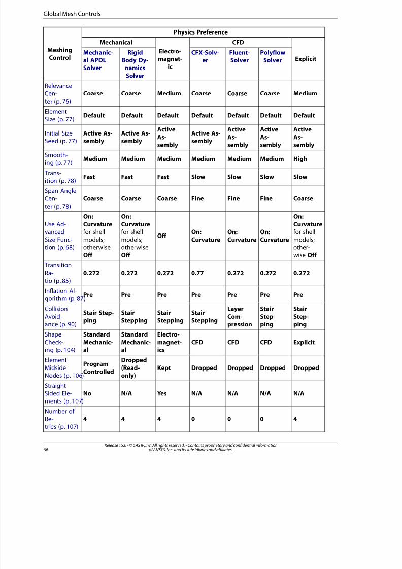
8/10/2019 ANSYS Meshing Users Guide
http://slidepdf.com/reader/full/ansys-meshing-users-guide 74/491
Physics Preference
Meshing
Control Explicit
CFD
Electro-magnet-
ic
Mechanical
PolyflowSolver
Fluent-Solver
CFX-Solv-er
RigidBody Dy-
namics
Solver
Mechanic-al APDLSolver
MediumCoarseCoarseCoarseMediumCoarseCoarseRelevanceCen-
ter (p. 76)
DefaultDefaultDefaultDefaultDefaultDefaultDefaultElement
Size (p. 77)
Active
As-sembly
Active
As-sembly
Active
As-sembly
Active As-sembly
Active
As-sembly
Active As-sembly
Active As-sembly
Initial SizeSeed (p. 77)
HighMediumMediumMediumMediumMediumMediumSmooth-
ing (p. 77)
SlowSlowSlowSlowFastFastFast
Trans-
ition (p. 78)
CoarseFineFineFineCoarseCoarseCoarseSpan AngleCen-
ter (p. 78)
On:
CurvatureOn:Curvature
On:Curvature
On:Curvature
Off
On:
Curvature
On:
CurvatureUse Ad-vanced for shellfor shellfor shellSize Func-tion (p. 68)
models;models;models;other-
wise Off
otherwise
Off
otherwise
Off
0.2720.2720.2720.770.2720.2720.272 TransitionRa-
tio (p. 85)
PrePrePrePrePrePrePreInflation Al-
gorithm (p. 87)
Stair
Step-ping
Stair
Step-ping
Layer
Com-pression
StairStepping
StairStepping
StairStepping
Stair Step-ping
Collision
Avoid-ance (p. 90)
ExplicitCFDCFDCFD
Electro-
magnet-ics
Standard
Mechanic-al
Standard
Mechanic-al
Shape
Check-ing (p. 104)
DroppedDroppedDroppedDroppedKeptDropped(Read-only)
ProgramControlled
ElementMidsideNodes (p. 106)
N/AN/AN/AN/AYesN/ANoStraightSided Ele-ments (p. 107)
4000444Number of Re-tries (p. 107)
Release 15.0 - © SAS IP, Inc. All rights reserved. - Contains proprietary and confidential informationof ANSYS, Inc. and its subsidiaries and affiliates.66
Global Mesh Controls
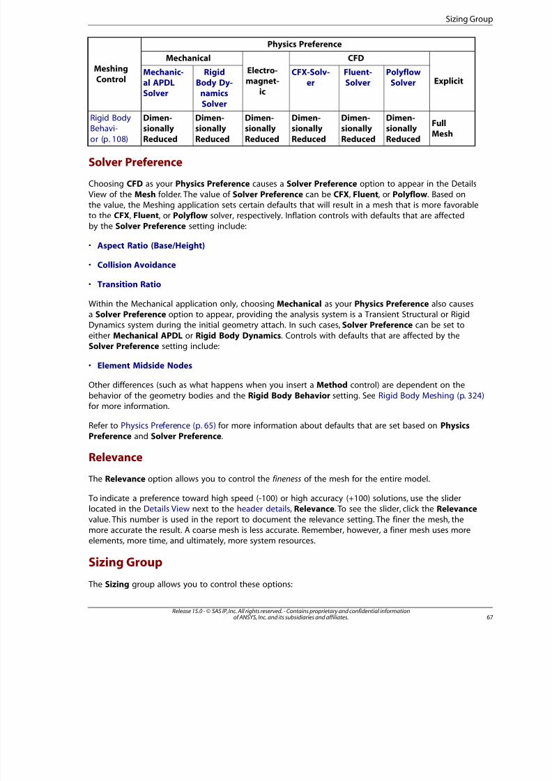
8/10/2019 ANSYS Meshing Users Guide
http://slidepdf.com/reader/full/ansys-meshing-users-guide 75/491
Physics Preference
Meshing
Control Explicit
CFD
Electro-magnet-
ic
Mechanical
PolyflowSolver
Fluent-Solver
CFX-Solv-er
RigidBody Dy-
namics
Solver
Mechanic-al APDLSolver
FullMesh
Dimen-sionally
Reduced
Dimen-sionally
Reduced
Dimen-sionally
Reduced
Dimen-sionally
Reduced
Dimen-sionally
Reduced
Dimen-sionally
Reduced
Rigid BodyBehavi-
or (p. 108)
Solver Preference
Choosing CFD as your Physics Preference causes a Solver Preference option to appear in the Details
View of the Mesh folder. The value of Solver Preference can be CFX, Fluent, or Polyflow. Based onthe value, the Meshing application sets certain defaults that will result in a mesh that is more favorableto the CFX, Fluent, or Polyflow solver, respectively. Inflation controls with defaults that are affectedby the Solver Preference setting include:
• Aspect Ratio (Base/Height)
• Collision Avoidance
• Transition Ratio
Within the Mechanical application only, choosing Mechanical as your Physics Preference also causesa Solver Preference option to appear, providing the analysis system is a Transient Structural or RigidDynamics system during the initial geometry attach. In such cases, Solver Preference can be set to
either Mechanical APDL or Rigid Body Dynamics. Controls with defaults that are affected by theSolver Preference setting include:
• Element Midside Nodes
Other differences (such as what happens when you insert a Method control) are dependent on the
behavior of the geometry bodies and the Rigid Body Behavior setting. See Rigid Body Meshing (p. 324)for more information.
Refer to Physics Preference (p. 65) for more information about defaults that are set based on Physics
Preference and Solver Preference.
Relevance
The Relevance option allows you to control the fineness of the mesh for the entire model.
To indicate a preference toward high speed (-100) or high accuracy (+100) solutions, use the sliderlocated in the Details View next to the header details, Relevance. To see the slider, click the Relevance
value. This number is used in the report to document the relevance setting. The finer the mesh, themore accurate the result. A coarse mesh is less accurate. Remember, however, a finer mesh uses moreelements, more time, and ultimately, more system resources.
Sizing Group
The Sizing group allows you to control these options:
67Release 15.0 - © SAS IP, Inc. All rights reserved. - Contains proprietary and confidential informationof ANSYS, Inc. and its subsidiaries and affiliates.
Sizing Group
8/10/2019 ANSYS Meshing Users Guide
http://slidepdf.com/reader/full/ansys-meshing-users-guide 76/491
Use Advanced Size FunctionRelevance Center
Element SizeInitial Size SeedSmoothing
TransitionSpan Angle CenterMinimum Edge Length
Use Advanced Size Function
The Use Advanced Size Function option provides greater control over sizing functions. Advanced sizefunctions control the following properties:
• Angles between normals for adjacent mesh elements (curvature-type size functions)
• Number of mesh elements employed in the gaps between two geometric entities (proximity-typesize function)
• Gradation between minimum and maximum sizes based on a specified growth rate (all size functions)
Options for Use Advanced Size Function are Off , On: Proximity and Curvature, On: Proximity, On:Curvature and On: Fixed. The default is Off , unless Physics Preference (p. 65) is set to CFD, in which
case the default is On: Curvature. The option you choose determines which refinement mechanismsare activated in the Advanced Size Function, as described in the following sections.
Controls that are common to all types of advanced size function include Min Size /Proximity Min Size,Max Face Size, Max Size, and Growth Rate. The Min Size /Proximity Min Size and Max Size specific-
ations represent, respectively, the global minimum and global maximum allowable element size. TheMax Face Size specification represents the global maximum allowable size of the elements created bythe free surface meshers of the supported methods. The Growth Rate represents the increase in element
edge length with each succeeding layer of elements from the edge or face. For example, a growth rateof 1.2 results in a 20% increase in element edge length with each succeeding layer of elements.
Advanced Size Function options are applicable to the following mesh methods:
Volume Meshing:
• General Sweep (Surface mesh only)
• Thin Sweep (Surface mesh only)
• Hex Dominant (Surface mesh only)
• Patch Conforming Tetrahedron
• Patch Independent Tetrahedron
• MultiZone
Release 15.0 - © SAS IP, Inc. All rights reserved. - Contains proprietary and confidential informationof ANSYS, Inc. and its subsidiaries and affiliates.68
Global Mesh Controls
8/10/2019 ANSYS Meshing Users Guide
http://slidepdf.com/reader/full/ansys-meshing-users-guide 77/491
• Assembly meshing algorithms (CutCell and Tetrahedrons)
Note
• The Advanced Size Function controls are passed to the Patch Independent Tetrahedron method.
That is, the Patch Independent Tetrahedron method does not use the same Advanced SizeFunction algorithms; rather, this method interprets the controls and uses internal algorithms
to respect the user settings.
• The General Sweep, Thin Sweep, and Hex Dominant mesh methods use the Advanced SizeFunction in the creation of the surface mesh, but the volume mesh does not use them.
Surface Meshing:
• Quad Dominant
• All Triangles
• MultiZone Quad/Tri
Note
For an overview of how using the Advanced Size Function influences mesh distribution, referto Understanding the Influence of the Advanced Size Function (p. 61).
Advanced Size Function topics include:Curvature Size Function
Proximity Size FunctionFixed Size Function
Specifying Size Function Options
Curvature Size Function
The curvature size function examines curvature on edges and faces and computes element sizes on
these entities such that the size will not violate the maximum size or the curvature normal angle, whichare either automatically computed by the mesher or defined by the user.
The curvature size function is defined by the following properties:
• Curvature Normal Angle
• Min Size
• Max Face Size
• Max Size
• Growth Rate
The Curvature Normal Angle is the maximum allowable angle that one element edge is allowed to
span.
69Release 15.0 - © SAS IP, Inc. All rights reserved. - Contains proprietary and confidential informationof ANSYS, Inc. and its subsidiaries and affiliates.
Sizing Group
8/10/2019 ANSYS Meshing Users Guide
http://slidepdf.com/reader/full/ansys-meshing-users-guide 78/491
For information about valid ranges and defaults for the size function controls discussed in this section,see Specifying Size Function Options (p. 71).
Proximity Size Function
The proximity size function allows you to specify the minimum number of element layers created inregions that constitute “gaps” in the model. For the purposes of specifying a proximity size function, a“gap” is defined in one of two ways:
• The internal volumetric region between two faces
• The area between two opposing boundary edges of a face
The proximity size function is defined by the following properties:
• Num Cells Across Gap
• Proximity Size Function Sources (assembly meshing algorithms only)
• Min Size
• Proximity Min Size
• Max Face Size
• Max Size
• Growth Rate
The Num Cells Across Gap is the number of layers of elements to be generated in the gaps. ProximitySize Function Sources determines which regions of proximity are considered in calculations. ProximityMin Size provides greater control over the size function, as it allows you to specify a minimum size for
proximity size function calculations in addition to the minimum size that is specified for Min Size.
Note
The proximity size function does not recognize the proximity between certain entities incases involving voids in a model. For example, the proximity between a vertex and an edge
on a face in 2D (below left) is ignored if the triangle is a void in the rectangle. Similarly, theproximity between a vertex or edge and a face in 3D (below right) is ignored if the prismand the block are voids in a larger domain. The two-headed arrows in the figure indicate theareas where proximity is ignored.
Release 15.0 - © SAS IP, Inc. All rights reserved. - Contains proprietary and confidential informationof ANSYS, Inc. and its subsidiaries and affiliates.70
Global Mesh Controls
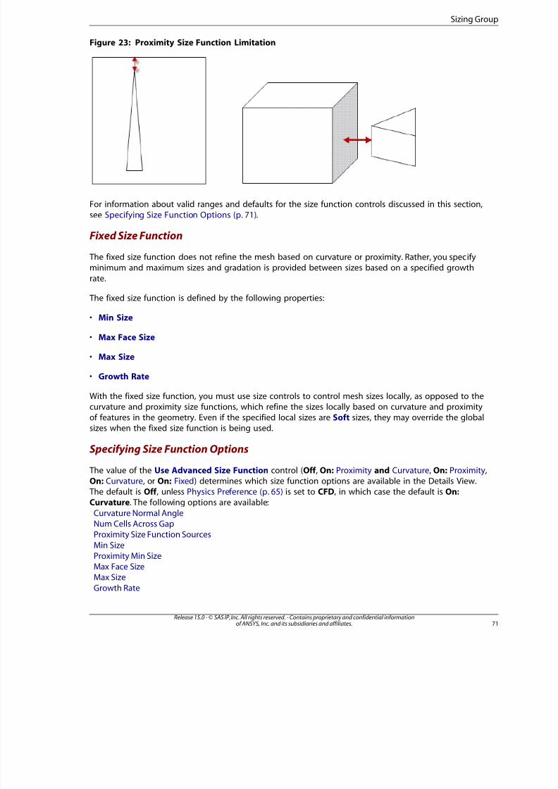
8/10/2019 ANSYS Meshing Users Guide
http://slidepdf.com/reader/full/ansys-meshing-users-guide 79/491
Figure 23: Proximity Size Function Limitation
For information about valid ranges and defaults for the size function controls discussed in this section,see Specifying Size Function Options (p. 71).
Fixed Size Function
The fixed size function does not refine the mesh based on curvature or proximity. Rather, you specifyminimum and maximum sizes and gradation is provided between sizes based on a specified growth
rate.
The fixed size function is defined by the following properties:
• Min Size
• Max Face Size
• Max Size
• Growth Rate
With the fixed size function, you must use size controls to control mesh sizes locally, as opposed to thecurvature and proximity size functions, which refine the sizes locally based on curvature and proximityof features in the geometry. Even if the specified local sizes are Soft sizes, they may override the globalsizes when the fixed size function is being used.
Specifying Size Function Options
The value of the Use Advanced Size Function control (Off , On: Proximity and Curvature, On: Proximity,On: Curvature, or On: Fixed) determines which size function options are available in the Details View.
The default is Off , unless Physics Preference (p. 65) is set to CFD, in which case the default is On:Curvature. The following options are available:
Curvature Normal AngleNum Cells Across GapProximity Size Function Sources
Min SizeProximity Min SizeMax Face SizeMax Size
Growth Rate
7Release 15.0 - © SAS IP, Inc. All rights reserved. - Contains proprietary and confidential informationof ANSYS, Inc. and its subsidiaries and affiliates.
Sizing Group
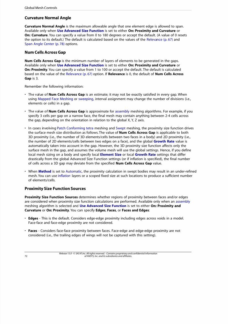
8/10/2019 ANSYS Meshing Users Guide
http://slidepdf.com/reader/full/ansys-meshing-users-guide 80/491
Curvature Normal Angle
Curvature Normal Angle is the maximum allowable angle that one element edge is allowed to span.Available only when Use Advanced Size Function is set to either On: Proximity and Curvature or
On: Curvature. You can specify a value from 0 to 180 degrees or accept the default. (A value of 0 resetsthe option to its default.) The default is calculated based on the values of the Relevance (p. 67) andSpan Angle Center (p. 78) options.
Num Cells Across Gap
Num Cells Across Gap is the minimum number of layers of elements to be generated in the gaps.Available only when Use Advanced Size Function is set to either On: Proximity and Curvature orOn: Proximity. You can specify a value from 1 to 100 or accept the default. The default is calculatedbased on the value of the Relevance (p. 67) option. If Relevance is 0, the default of Num Cells Across
Gap is 3.
Remember the following information:
• The value of Num Cells Across Gap is an estimate; it may not be exactly satisfied in every gap. When
using Mapped Face Meshing or sweeping, interval assignment may change the number of divisions (i.e.,elements or cells) in a gap.
• The value of Num Cells Across Gap is approximate for assembly meshing algorithms. For example, if you
specify 3 cells per gap on a narrow face, the final mesh may contain anything between 2-4 cells acrossthe gap, depending on the orientation in relation to the global X, Y, Z axis.
• In cases involving Patch Conforming tetra meshing and Swept meshing, the proximity size function drivesthe surface mesh size distribution as follows. The value of Num Cells Across Gap is applicable to both
3D proximity (i.e., the number of 3D elements/cells between two faces in a body) and 2D proximity (i.e.,the number of 2D elements/cells between two edges on a face), and the global Growth Rate value isautomatically taken into account in the gap. However, the 3D proximity size function affects only the
surface mesh in the gap, and assumes the volume mesh will use the global settings. Hence, if you definelocal mesh sizing on a body and specify local Element Size or local Growth Rate settings that differdrastically from the global Advanced Size Function settings (or if inflation is specified), the final numberof cells across a 3D gap may deviate from the specified Num Cells Across Gap value.
• When Method is set to Automatic, the proximity calculation in swept bodies may result in an under-refinedmesh. You can use inflation layers or a scoped fixed size at such locations to produce a sufficient numberof elements/cells.
Proximity Size Function Sources
Proximity Size Function Sources determines whether regions of proximity between faces and/or edges
are considered when proximity size function calculations are performed. Available only when an assemblymeshing algorithm is selected and Use Advanced Size Function is set to either On: Proximity andCurvature or On: Proximity. You can specify Edges, Faces, or Faces and Edges:
• Edges - This is the default. Considers edge-edge proximity including edges across voids in a model.Face-face and face-edge proximity are not considered.
• Faces - Considers face-face proximity between faces. Face-edge and edge-edge proximity are not
considered (i.e., the trailing edges of wings will not be captured with this setting).
Release 15.0 - © SAS IP, Inc. All rights reserved. - Contains proprietary and confidential informationof ANSYS, Inc. and its subsidiaries and affiliates.72
Global Mesh Controls
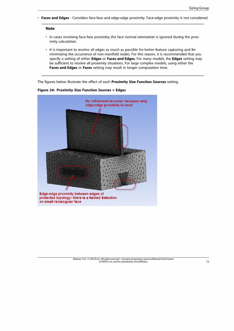
8/10/2019 ANSYS Meshing Users Guide
http://slidepdf.com/reader/full/ansys-meshing-users-guide 81/491
• Faces and Edges - Considers face-face and edge-edge proximity. Face-edge proximity is not considered.
Note
• In cases involving face-face proximity, the face normal orientation is ignored during the prox-
imity calculation.
• It is important to resolve all edges as much as possible for better feature capturing and forminimizing the occurrence of non-manifold nodes. For this reason, it is recommended that you
specify a setting of either Edges or Faces and Edges. For many models, the Edges setting maybe sufficient to resolve all proximity situations. For large complex models, using either theFaces and Edges or Faces setting may result in longer computation time.
The figures below illustrate the effect of each Proximity Size Function Sources setting.
Figure 24: Proximity Size Function Sources = Edges
73Release 15.0 - © SAS IP, Inc. All rights reserved. - Contains proprietary and confidential informationof ANSYS, Inc. and its subsidiaries and affiliates.
Sizing Group
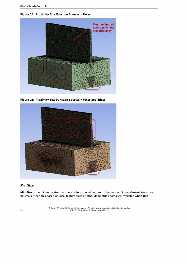
8/10/2019 ANSYS Meshing Users Guide
http://slidepdf.com/reader/full/ansys-meshing-users-guide 82/491
Figure 25: Proximity Size Function Sources = Faces
Figure 26: Proximity Size Function Sources = Faces and Edges
Min Size
Min Size is the minimum size that the size function will return to the mesher. Some element sizes maybe smaller than this based on local feature sizes or other geometric anomalies. Available when Use
Release 15.0 - © SAS IP, Inc. All rights reserved. - Contains proprietary and confidential informationof ANSYS, Inc. and its subsidiaries and affiliates.74
Global Mesh Controls
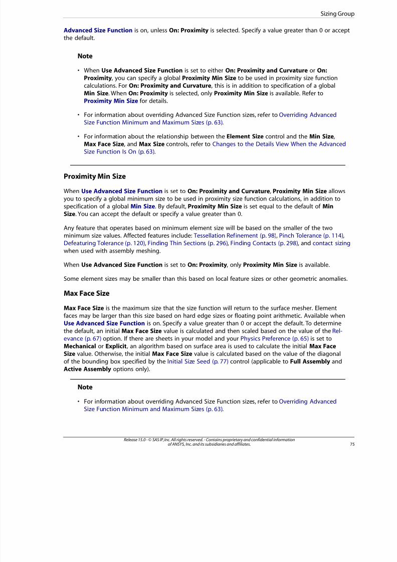
8/10/2019 ANSYS Meshing Users Guide
http://slidepdf.com/reader/full/ansys-meshing-users-guide 83/491
Advanced Size Function is on, unless On: Proximity is selected. Specify a value greater than 0 or acceptthe default.
Note
• When Use Advanced Size Function is set to either On: Proximity and Curvature or On:Proximity, you can specify a global Proximity Min Size to be used in proximity size function
calculations. For On: Proximity and Curvature, this is in addition to specification of a globalMin Size. When On: Proximity is selected, only Proximity Min Size is available. Refer toProximity Min Size for details.
• For information about overriding Advanced Size Function sizes, refer to Overriding AdvancedSize Function Minimum and Maximum Sizes (p. 63).
• For information about the relationship between the Element Size control and the Min Size,Max Face Size, and Max Size controls, refer to Changes to the Details View When the AdvancedSize Function Is On (p. 63).
Proximity Min Size
When Use Advanced Size Function is set to On: Proximity and Curvature, Proximity Min Size allowsyou to specify a global minimum size to be used in proximity size function calculations, in addition tospecification of a global Min Size. By default, Proximity Min Size is set equal to the default of MinSize. You can accept the default or specify a value greater than 0.
Any feature that operates based on minimum element size will be based on the smaller of the twominimum size values. Affected features include: Tessellation Refinement (p. 98), Pinch Tolerance (p. 114),Defeaturing Tolerance (p. 120), Finding Thin Sections (p. 296), Finding Contacts (p. 298), and contact sizing
when used with assembly meshing.
When Use Advanced Size Function is set to On: Proximity, only Proximity Min Size is available.
Some element sizes may be smaller than this based on local feature sizes or other geometric anomalies.
Max Face Size
Max Face Size is the maximum size that the size function will return to the surface mesher. Elementfaces may be larger than this size based on hard edge sizes or floating point arithmetic. Available whenUse Advanced Size Function is on. Specify a value greater than 0 or accept the default. To determine
the default, an initial Max Face Size value is calculated and then scaled based on the value of the Rel-evance (p. 67) option. If there are sheets in your model and your Physics Preference (p. 65) is set toMechanical or Explicit, an algorithm based on surface area is used to calculate the initial Max Face
Size value. Otherwise, the initial Max Face Size value is calculated based on the value of the diagonalof the bounding box specified by the Initial Size Seed (p. 77) control (applicable to Full Assembly andActive Assembly options only).
Note
• For information about overriding Advanced Size Function sizes, refer to Overriding AdvancedSize Function Minimum and Maximum Sizes (p. 63).
75Release 15.0 - © SAS IP, Inc. All rights reserved. - Contains proprietary and confidential informationof ANSYS, Inc. and its subsidiaries and affiliates.
Sizing Group

8/10/2019 ANSYS Meshing Users Guide
http://slidepdf.com/reader/full/ansys-meshing-users-guide 84/491
• If you parameterize the Element Size or Max Face Size control when toggling the AdvancedSize Function on and off, the parameterization of one control will have no effect on the other.
However, the value of one control will be copied to the other if it is not the default. For moreinformation about the relationship between the Element Size control and the Min Size, MaxFace Size, and Max Size controls, refer to Changes to the Details View When the AdvancedSize Function Is On (p. 63).
• Max Face Size is unavailable for assembly meshing algorithms.
Max Size
Max Size is the maximum size that the size function will return to the mesher. Available when UseAdvanced Size Function is on. Specify a value greater than 0 or accept the default.
Note
• The Max Size option is hidden if there are no solids in your model.
• For information about overriding Advanced Size Function sizes, refer to Overriding AdvancedSize Function Minimum and Maximum Sizes (p. 63).
• For information about the relationship between the Element Size control and the Min Size,Max Face Size, and Max Size controls, refer to Changes to the Details View When the AdvancedSize Function Is On (p. 63).
Growth Rate
Growth Rate represents the increase in element edge length with each succeeding layer of elements.
For example, a growth rate of 1.2 results in a 20% increase in element edge length with each succeedinglayer of elements. Available when Use Advanced Size Function is on. Specify a value from 1 to 5 oraccept the default. The default is calculated based on the values of the Relevance (p. 67) and Trans-
ition (p. 78) options.
Note
For sheet models, the Details View does not display the default value of Growth Rate.
Relevance Center
Relevance Center sets the gauge of the Relevance slider control in the Default group. Options areCoarse, Medium, and Fine. The default value can be set automatically according to the Physics Pref-erence setting as described above under the Default Group.
Release 15.0 - © SAS IP, Inc. All rights reserved. - Contains proprietary and confidential informationof ANSYS, Inc. and its subsidiaries and affiliates.76
Global Mesh Controls

8/10/2019 ANSYS Meshing Users Guide
http://slidepdf.com/reader/full/ansys-meshing-users-guide 85/491
Element Size
Element Size allows you to specify the element size used for the entire model. This size will be usedfor all edge, face, and body meshing. This option does not appear when Use Advanced Size Func-tion (p. 68) is on.
Note
If you parameterize the Element Size or Max Face Size control when toggling the AdvancedSize Function on and off, the parameterization of one control will have no effect on theother. However, the value of one control will be copied to the other if it is not the default.
For more information about the relationship between the Element Size control and the MinSize, Max Face Size, and Max Size controls, refer to Changes to the Details View When theAdvanced Size Function Is On (p. 63).
Initial Size Seed
Initial Size Seed allows you to control the initial seeding of the mesh size for each part.
• Active Assembly (default) bases the initial seeding on the diagonal of the bounding box that encloses
only parts that are unsuppressed (“active” parts). With this choice, the mesh could change as you suppreand unsuppress parts because the bounding box grows and shrinks.
• Full Assembly bases the initial seeding on the diagonal of the bounding box that encloses all assembly
parts regardless of the number of suppressed parts. As a result, the mesh never changes due to partsuppression.
• Part bases the initial seeding on the diagonal of the bounding box that encloses each particular individpart as it is meshed. The mesh never changes due to part suppression. This option typically leads to a
finer mesh and is recommended for situations where the fineness of an individual part mesh is importan
relative to the overall size of the part in the assembly. This option is not valid when Use Advanced SizeFunction (p. 68) is on.
Note
For information on how suppressing and unsuppressing bodies can affect a mesh, refer toGenerating Mesh (p. 354).
Smoothing
Smoothing attempts to improve element quality by moving locations of nodes with respect to surround-
ing nodes and elements. The Low, Medium, or High option controls the number of smoothing iterationsalong with the threshold metric where the mesher will start smoothing.
Note
In cases in which Smoothing is set to High and an assembly meshing algorithm is beingused, additional smoothing of inflation layers occurs. This may slow down the prism generationprocess. Refer to The Assembly Meshing Workflow (p. 276) for additional details on Smoothingsettings and their effects on assembly meshing.
77Release 15.0 - © SAS IP, Inc. All rights reserved. - Contains proprietary and confidential informationof ANSYS, Inc. and its subsidiaries and affiliates.
Sizing Group
8/10/2019 ANSYS Meshing Users Guide
http://slidepdf.com/reader/full/ansys-meshing-users-guide 86/491
Transition
Transition affects the rate at which adjacent elements will grow. Slow produces smooth transitionswhile Fast produces more abrupt transitions.
Note
When Use Advanced Size Function (p. 68) is on, the Transition option is hidden for sheetmodels. For assemblies containing both sheets and solids, the Transition option appearsbut its value is ignored for the sheet geometry.
Span Angle Center
Span Angle Center sets the goal for curvature based refinement. The mesh will subdivide in curvedregions until the individual elements span this angle. The following choices are available:
• Coarse - 91o to 60
o
• Medium - 75o
to 24o
• Fine - 36o to 12
o
Minimum Edge Length
Minimum Edge Length provides a read-only indication of the smallest edge length in the model.
Inflation Group
Inflation is useful for CFD boundary layer resolution, electromagnetic air gap resolution or resolving
high stress concentrations for structures. Inflation is supported for the following mesh methods:
Volume Meshing:
• Patch Conforming
• Patch Independent
• Sweep
Note
Inflation is supported for the sweep mesh method only when the Src/Trg Selection optionis set to either Manual Source or Manual Source and Target.
• MultiZone
• Assembly meshing algorithms (CutCell and Tetrahedrons)
Surface Meshing:
• Quad Dominant
Release 15.0 - © SAS IP, Inc. All rights reserved. - Contains proprietary and confidential informationof ANSYS, Inc. and its subsidiaries and affiliates.78
Global Mesh Controls
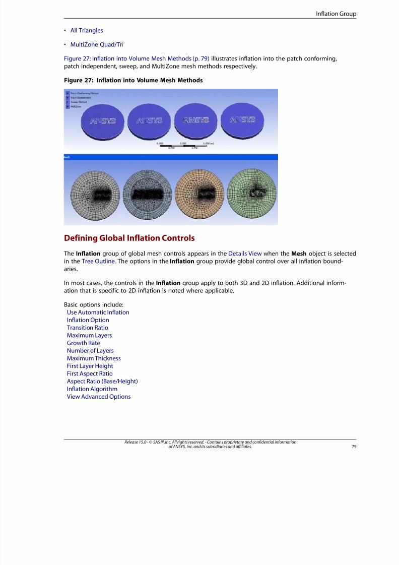
8/10/2019 ANSYS Meshing Users Guide
http://slidepdf.com/reader/full/ansys-meshing-users-guide 87/491
• All Triangles
• MultiZone Quad/Tri
Figure 27: Inflation into Volume Mesh Methods (p. 79) illustrates inflation into the patch conforming,patch independent, sweep, and MultiZone mesh methods respectively.
Figure 27: Inflation into Volume Mesh Methods
Defining Global Inflation Controls
The Inflation group of global mesh controls appears in the Details View when the Mesh object is selectedin the Tree Outline. The options in the Inflation group provide global control over all inflation bound-
aries.
In most cases, the controls in the Inflation group apply to both 3D and 2D inflation. Additional inform-ation that is specific to 2D inflation is noted where applicable.
Basic options include:Use Automatic InflationInflation Option Transition Ratio
Maximum LayersGrowth RateNumber of Layers
Maximum ThicknessFirst Layer HeightFirst Aspect RatioAspect Ratio (Base/Height)
Inflation AlgorithmView Advanced Options
79Release 15.0 - © SAS IP, Inc. All rights reserved. - Contains proprietary and confidential informationof ANSYS, Inc. and its subsidiaries and affiliates.
Inflation Group
8/10/2019 ANSYS Meshing Users Guide
http://slidepdf.com/reader/full/ansys-meshing-users-guide 88/491
Defining Local Inflation Controls
In addition to setting global inflation controls, you can use local (scoped) inflation controls to applyinflation to specific boundaries. In most cases, the values that you set globally will be populated to thelocal inflation controls. If you subsequently make changes to the local inflation settings, the local settings
will override the global settings. For details, refer to Inflation Control (p. 217).
Inflation and Mesh Method ControlsFor steps to follow to assign inflation depending on the selected mesh method, refer to Inflation Con-trols (p. 316). For general information on applying inflation controls in combination with the variousmesh method controls, refer to "Meshing: Mesh Control Interaction Tables" (p. 345).
Use Automatic Inflation
You can set the Use Automatic Inflation control so that inflation boundaries are selected automatically
depending on whether or not they are members of Named Selections groups. The following optionsare available:
None
Program ControlledAll Faces in Chosen Named Selection
Remember the following information when using inflation:
• Automatic inflation is supported only for 3D inflation on volume models. It is not supported for 2D inflation
on shell models. You cannot select Program Controlled (p. 81) or All Faces in Chosen Named Selec-tion (p. 82) for the Use Automatic Inflation option to mesh a 2D model. To apply 2D inflation on a shellmodel, use local inflation mesh controls instead.
• In the following scenarios, using inflation results in automatic suppression of the refinement control:
– When automatic inflation (either Program Controlled (p. 81) or All Faces in Chosen Named Selec-tion (p. 82)) is used with refinement in the same model
– When local inflation is used with refinement in the same body or in the same part
• In general, using a mixture of local inflation and automatic inflation within the same part is not recommen-
ded . When you mix local and automatic inflation, the local inflation settings will be used for the bodiesto which they are applied. The automatic inflation settings will create inflation only on those bodies that
do not have local inflation applied to them. The automatic inflation settings will ignore all bodies and allattached faces to which local inflation settings are applied.
If an assembly meshing algorithm is being used, a mixture of local and automatic inflation is not
supported . Refer to The Assembly Meshing Workflow (p. 276) for details.
None
If you select None, inflation boundaries are not selected globally. Instead, the inflation boundaries thatyou identify using the local inflation mesh controls are used. This is the default.
Release 15.0 - © SAS IP, Inc. All rights reserved. - Contains proprietary and confidential informationof ANSYS, Inc. and its subsidiaries and affiliates.80
Global Mesh Controls
8/10/2019 ANSYS Meshing Users Guide
http://slidepdf.com/reader/full/ansys-meshing-users-guide 89/491
Program Controlled
Program Controlled inflation operates differently depending on whether meshing occurs at thepart/body level or assembly level.
Note
Program Controlled inflation is only supported for 3D models.
Program Controlled Inflation for Part/Body Level Meshing
If you are using a mesh method that operates at the part/body level and you select Program Controlledinflation, all faces in the model are selected to be inflation boundaries, except for the following:
• Faces in Named Selection(s)
Note
By default, faces in Named Selections are not selected to be inflation boundaries whenUse Automatic Inflation is set to Program Controlled. However, you can select specificNamed Selections to be included in Program Controlled inflation. For details, see the
discussion of Named Selections and Program Controlled inflation in the Mechanical help.
• Faces in Contact region(s)
• Faces in Symmetry definition
• Faces that belong to a part/body that has a mesh method defined on it that does not support 3D inflatidefinitions (i.e., mesh method is set to Sweep or Hex Dominant)
• Faces in sheet bodies
• Faces on bodies that have manual inflation controls
When Program Controlled automatic inflation is used for part/body level meshing, the mesher inflatesin the following manner:
• For single body parts, the face will always inflate into the body.
• For multibody parts with a mix of fluid and solid parts:
– Faces on fluid region will inflate into fluid region; solid region will not be inflated.
– Faces on parts of the same material will not be inflated.
• For parts of the same material, shared faces will not be inflated.
The manner in which inflation is applied depends on values that you enter for the following options:
• Inflation Option (p. 83)
• Inflation Algorithm (p. 87)
8Release 15.0 - © SAS IP, Inc. All rights reserved. - Contains proprietary and confidential informationof ANSYS, Inc. and its subsidiaries and affiliates.
Inflation Group
8/10/2019 ANSYS Meshing Users Guide
http://slidepdf.com/reader/full/ansys-meshing-users-guide 90/491
• View Advanced Options (p. 90)
Note
When Program Controlled automatic inflation is being used for part/body level meshing,
you can view the surfaces that have been selected for inflation by using the Show ProgramControlled Inflation Surfaces feature.
Program Controlled Inflation for Assembly Level Meshing
If you are using an assembly meshing algorithm and you select Program Controlled inflation, all faces
in the model are selected to be inflation boundaries, except for the following:
• Faces in Named Selection(s)
Note
By default, faces in Named Selections are not selected to be inflation boundaries whenUse Automatic Inflation is set to Program Controlled. However, you can select specific
Named Selections to be included in Program Controlled inflation. For details, see thediscussion of Named Selections and Program Controlled inflation in the Mechanical help.
• Faces in Symmetry definition
When Program Controlled automatic inflation is used for assembly level meshing, the mesher inflatesin the following manner:
• All fluid bodies, either real or virtual, will be inflated based on the rules above. Solid bodies will not be
inflated (where a “solid” body is a volume body with Fluid/Solid set to Solid).
Note
The Show Program Controlled Inflation Surfaces feature is not supported for assemblymeshing algorithms.
All Faces in Chosen Named Selection
If you select All Faces in Chosen Named Selection, a Named Selection field is displayed to let youscope inflation to the Named Selection. The manner in which inflation is applied to the Named Selections
group depends on values that you enter for the following options:
• Inflation Option (p. 83)
• Inflation Algorithm (p. 87)
Release 15.0 - © SAS IP, Inc. All rights reserved. - Contains proprietary and confidential informationof ANSYS, Inc. and its subsidiaries and affiliates.82
Global Mesh Controls

8/10/2019 ANSYS Meshing Users Guide
http://slidepdf.com/reader/full/ansys-meshing-users-guide 91/491
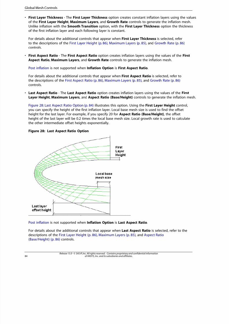
8/10/2019 ANSYS Meshing Users Guide
http://slidepdf.com/reader/full/ansys-meshing-users-guide 92/491
• First Layer Thickness - The First Layer Thickness option creates constant inflation layers using the valuesof the First Layer Height, Maximum Layers, and Growth Rate controls to generate the inflation mesh.
Unlike inflation with the Smooth Transition option, with the First Layer Thickness option the thicknessof the first inflation layer and each following layer is constant.
For details about the additional controls that appear when First Layer Thickness is selected, refer
to the descriptions of the First Layer Height (p. 86), Maximum Layers (p. 85), and Growth Rate (p. 86)controls.
• First Aspect Ratio - The First Aspect Ratio option creates inflation layers using the values of the First
Aspect Ratio, Maximum Layers, and Growth Rate controls to generate the inflation mesh.
Post inflation is not supported when Inflation Option is First Aspect Ratio.
For details about the additional controls that appear when First Aspect Ratio is selected, refer tothe descriptions of the First Aspect Ratio (p. 86), Maximum Layers (p. 85), and Growth Rate (p. 86)
controls.
• Last Aspect Ratio - The Last Aspect Ratio option creates inflation layers using the values of the FirstLayer Height, Maximum Layers, and Aspect Ratio (Base/Height) controls to generate the inflation mesh.
Figure 28: Last Aspect Ratio Option (p. 84) illustrates this option. Using the First Layer Height control,you can specify the height of the first inflation layer. Local base mesh size is used to find the offsetheight for the last layer. For example, if you specify 20 for Aspect Ratio (Base/Height), the offset
height of the last layer will be 0.2 times the local base mesh size. Local growth rate is used to calculatethe other intermediate offset heights exponentially.
Figure 28: Last Aspect Ratio Option
Post inflation is not supported when Inflation Option is Last Aspect Ratio.
For details about the additional controls that appear when Last Aspect Ratio is selected, refer to thedescriptions of the First Layer Height (p. 86), Maximum Layers (p. 85), and Aspect Ratio(Base/Height) (p. 86) controls.
Release 15.0 - © SAS IP, Inc. All rights reserved. - Contains proprietary and confidential informationof ANSYS, Inc. and its subsidiaries and affiliates.84
Global Mesh Controls
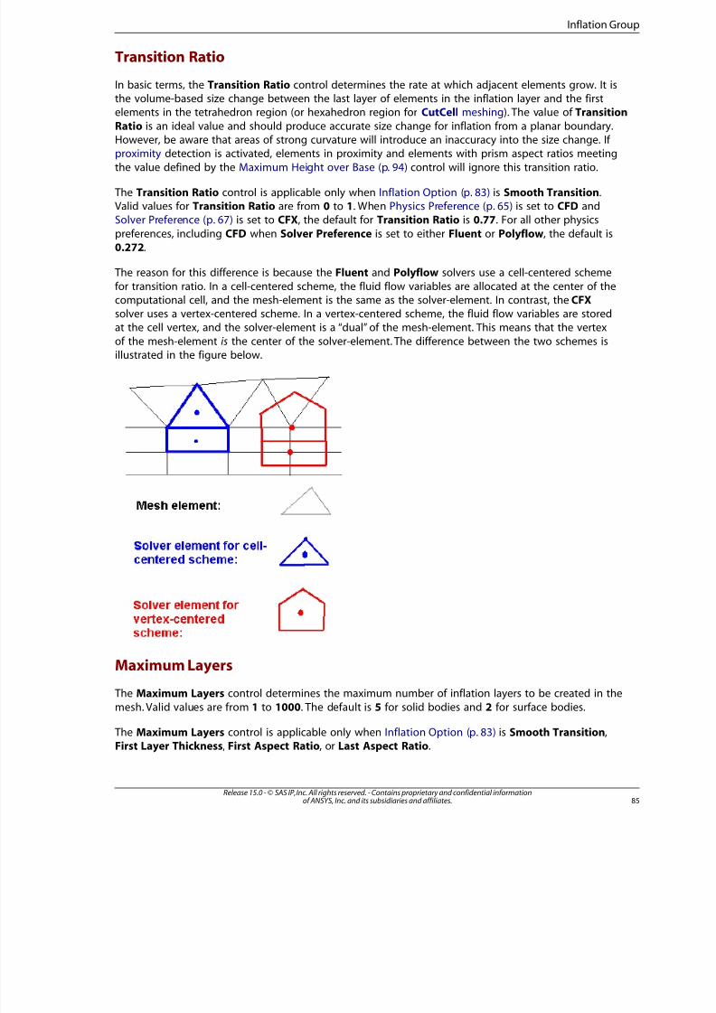
8/10/2019 ANSYS Meshing Users Guide
http://slidepdf.com/reader/full/ansys-meshing-users-guide 93/491
Transition Ratio
In basic terms, the Transition Ratio control determines the rate at which adjacent elements grow. It isthe volume-based size change between the last layer of elements in the inflation layer and the firstelements in the tetrahedron region (or hexahedron region for CutCell meshing). The value of Transition
Ratio is an ideal value and should produce accurate size change for inflation from a planar boundary.However, be aware that areas of strong curvature will introduce an inaccuracy into the size change. If
proximity detection is activated, elements in proximity and elements with prism aspect ratios meetingthe value defined by the Maximum Height over Base (p. 94) control will ignore this transition ratio.
The Transition Ratio control is applicable only when Inflation Option (p. 83) is Smooth Transition.Valid values for Transition Ratio are from 0 to 1. When Physics Preference (p. 65) is set to CFD andSolver Preference (p. 67) is set to CFX, the default for Transition Ratio is 0.77. For all other physics
preferences, including CFD when Solver Preference is set to either Fluent or Polyflow, the default is0.272.
The reason for this difference is because the Fluent and Polyflow solvers use a cell-centered scheme
for transition ratio. In a cell-centered scheme, the fluid flow variables are allocated at the center of thecomputational cell, and the mesh-element is the same as the solver-element. In contrast, the CFX
solver uses a vertex-centered scheme. In a vertex-centered scheme, the fluid flow variables are storedat the cell vertex, and the solver-element is a “dual” of the mesh-element. This means that the vertex
of the mesh-element is the center of the solver-element. The difference between the two schemes isillustrated in the figure below.
Maximum Layers
The Maximum Layers control determines the maximum number of inflation layers to be created in the
mesh. Valid values are from 1 to 1000. The default is 5 for solid bodies and 2 for surface bodies.
The Maximum Layers control is applicable only when Inflation Option (p. 83) is Smooth Transition,First Layer Thickness, First Aspect Ratio, or Last Aspect Ratio.
85Release 15.0 - © SAS IP, Inc. All rights reserved. - Contains proprietary and confidential informationof ANSYS, Inc. and its subsidiaries and affiliates.
Inflation Group

8/10/2019 ANSYS Meshing Users Guide
http://slidepdf.com/reader/full/ansys-meshing-users-guide 94/491
Growth Rate
The Growth Rate control determines the relative thickness of adjacent inflation layers. As you moveaway from the face to which the inflation control is applied, each successive layer is approximately onegrowth rate factor thicker than the previous one. Valid values are from 0.1 to 5.0. The default is 1.2.
The Growth Rate control is applicable only when Inflation Option (p. 83) is Smooth Transition, FirstLayer Thickness, Total Thickness, or First Aspect Ratio.
Number of Layers
The Number of Layers control determines the actual number of inflation layers in the mesh, except inplaces where layers are removed locally for reasons of improving mesh quality (for example, in areas
where inflation layers would otherwise collide with each other). Valid values are from 1 to 1000. Thedefault is 5 for solid bodies and 2 for surface bodies.
The Number of Layers control is applicable only when Inflation Option (p. 83) is Total Thickness.
Maximum Thickness
The Maximum Thickness control determines the desired thickness of the inflation layer. You must
enter a value for this control, and it must be greater than 0.
The Maximum Thickness control is applicable only when Inflation Option (p. 83) is Total Thickness.
First Layer Height
The First Layer Height control determines the height of the first inflation layer. This first inflation layerconsists of a single layer of prism elements that is formed against the faces of the inflation boundary.
You must enter a value for this control, and it must be greater than 0.
The First Layer Height control is applicable only when Inflation Option (p. 83) is First Layer Thicknessor Last Aspect Ratio.
First Aspect Ratio
By choosing the First Aspect Ratio option for the Inflation Option control, you can control the heightsof the inflation layers by defining the aspect ratio of the inflations that are extruded from the inflation
base. The aspect ratio is defined as the ratio of the local inflation base size to the inflation layer height.Use the First Aspect Ratio control to specify the first aspect ratio to be used. Enter a value greaterthan 0. The default is 5.
The First Aspect Ratio control is applicable only when Inflation Option (p. 83) is First Aspect Ratio.
Aspect Ratio (Base/Height)
By choosing the Last Aspect Ratio option for the Inflation Option control, you can control the heightsof the inflation layers by defining the aspect ratio of the inflations that are extruded from the inflationbase. The aspect ratio is defined as the ratio of the local inflation base size to the inflation layer height.Use the Aspect Ratio (Base/Height) control to specify the aspect ratio to be used. Enter a value between
0.5 and 20. The default is 1.5 when Solver Preference (p. 67) is CFX, and 3 when Solver Preference (p. 67)is Fluent or Polyflow.
Release 15.0 - © SAS IP, Inc. All rights reserved. - Contains proprietary and confidential informationof ANSYS, Inc. and its subsidiaries and affiliates.86
Global Mesh Controls
8/10/2019 ANSYS Meshing Users Guide
http://slidepdf.com/reader/full/ansys-meshing-users-guide 95/491
The Aspect Ratio (Base/Height) control is applicable only when Inflation Option (p. 83) is Last AspectRatio.
Inflation Algorithm
The Inflation Algorithm control determines which inflation algorithm will be used. Options for InflationAlgorithm are Pre and Post and are dependent upon the selected mesh method.
The following table shows which inflation algorithms are applicable to each mesh method. For inform-ation on how the inflation algorithm is handled when a combination of mesh methods is being used,
see Interactions Between Mesh Methods (p. 345).
Note
The Inflation Algorithm control is hidden when an assembly meshing algorithm is selected.Refer to The Assembly Meshing Workflow (p. 276) for details.
Inflation AlgorithmMesh Method
PostPreYes, 3DYes, 3DPatch Conforming
Tetrahedrons
Yes, 3DN/APatch Independ-ent Tetrahedrons
N/AN/AHex Dominant
N/AYes, 2D. Occurs in the following man-
ner: 1) source face is meshed with tri-
Sweep
angles, 2) inflation occurs on tri surfacemesh, and 3) source is swept. Intervals
on source and target are fixed.
N/A The value of Inflation Algorithm dis-plays as Pre but an O-grid-based al-
MultiZone
gorithm specific to MultiZone is used.As with the Pre inflation algorithm, themesh is inflated during the meshingprocess.
Yes, 2DN/AMultiZoneQuad/Tri
N/AYes, 2DQuad Dominant
N/AYes, 2DAll Triangles
Pre
When Pre is selected, the surface mesh will be inflated first, and then the rest of the volume mesh willbe generated. This is the default for all physics types.
Remember the following information:
• Inflation Algorithm must be set to Pre for the Previewing Inflation (p. 358) feature to work.
87Release 15.0 - © SAS IP, Inc. All rights reserved. - Contains proprietary and confidential informationof ANSYS, Inc. and its subsidiaries and affiliates.
Inflation Group
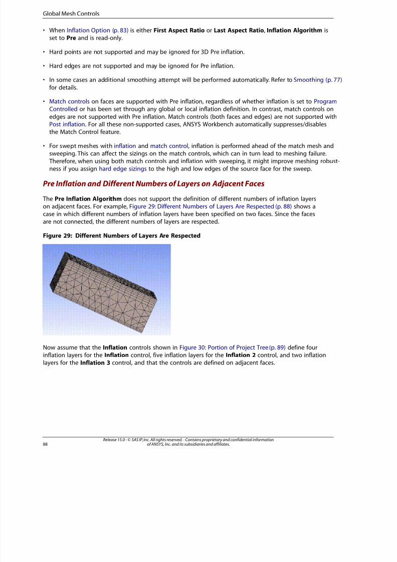
8/10/2019 ANSYS Meshing Users Guide
http://slidepdf.com/reader/full/ansys-meshing-users-guide 96/491
• When Inflation Option (p. 83) is either First Aspect Ratio or Last Aspect Ratio, Inflation Algorithm isset to Pre and is read-only.
• Hard points are not supported and may be ignored for 3D Pre inflation.
• Hard edges are not supported and may be ignored for Pre inflation.
• In some cases an additional smoothing attempt will be performed automatically. Refer to Smoothing (p. 77)
for details.
• Match controls on faces are supported with Pre inflation, regardless of whether inflation is set to ProgramControlled or has been set through any global or local inflation definition. In contrast, match controls on
edges are not supported with Pre inflation. Match controls (both faces and edges) are not supported withPost inflation. For all these non-supported cases, ANSYS Workbench automatically suppresses/disablesthe Match Control feature.
• For swept meshes with inflation and match control, inflation is performed ahead of the match mesh andsweeping. This can affect the sizings on the match controls, which can in turn lead to meshing failure. Therefore, when using both match controls and inflation with sweeping, it might improve meshing robust-ness if you assign hard edge sizings to the high and low edges of the source face for the sweep.
Pre Inflation and Different Numbers of Layers on Adjacent Faces
The Pre Inflation Algorithm does not support the definition of different numbers of inflation layerson adjacent faces. For example, Figure 29: Different Numbers of Layers Are Respected (p. 88) shows acase in which different numbers of inflation layers have been specified on two faces. Since the facesare not connected, the different numbers of layers are respected.
Figure 29: Different Numbers of Layers Are Respected
Now assume that the Inflation controls shown in Figure 30: Portion of Project Tree (p. 89) define four
inflation layers for the Inflation control, five inflation layers for the Inflation 2 control, and two inflationlayers for the Inflation 3 control, and that the controls are defined on adjacent faces.
Release 15.0 - © SAS IP, Inc. All rights reserved. - Contains proprietary and confidential informationof ANSYS, Inc. and its subsidiaries and affiliates.88
Global Mesh Controls
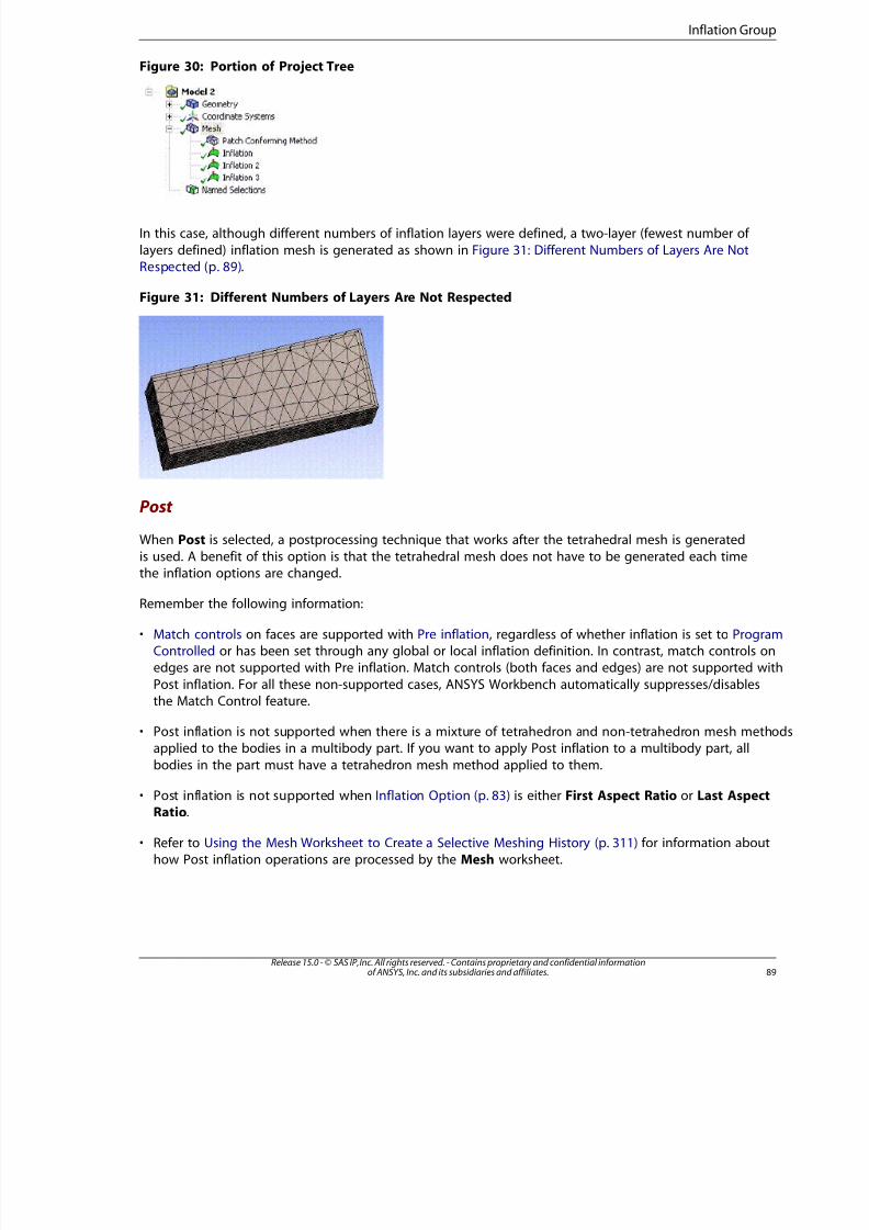
8/10/2019 ANSYS Meshing Users Guide
http://slidepdf.com/reader/full/ansys-meshing-users-guide 97/491
Figure 30: Portion of Project Tree
In this case, although different numbers of inflation layers were defined, a two-layer (fewest number of
layers defined) inflation mesh is generated as shown in Figure 31: Different Numbers of Layers Are NotRespected (p. 89).
Figure 31: Different Numbers of Layers Are Not Respected
Post
When Post is selected, a postprocessing technique that works after the tetrahedral mesh is generated
is used. A benefit of this option is that the tetrahedral mesh does not have to be generated each time
the inflation options are changed.
Remember the following information:
• Match controls on faces are supported with Pre inflation, regardless of whether inflation is set to PrograControlled or has been set through any global or local inflation definition. In contrast, match controls onedges are not supported with Pre inflation. Match controls (both faces and edges) are not supported wit
Post inflation. For all these non-supported cases, ANSYS Workbench automatically suppresses/disablesthe Match Control feature.
• Post inflation is not supported when there is a mixture of tetrahedron and non-tetrahedron mesh methoapplied to the bodies in a multibody part. If you want to apply Post inflation to a multibody part, all
bodies in the part must have a tetrahedron mesh method applied to them.
• Post inflation is not supported when Inflation Option (p. 83) is either First Aspect Ratio or Last AspectRatio.
• Refer to Using the Mesh Worksheet to Create a Selective Meshing History (p. 311) for information abouthow Post inflation operations are processed by the Mesh worksheet.
89Release 15.0 - © SAS IP, Inc. All rights reserved. - Contains proprietary and confidential informationof ANSYS, Inc. and its subsidiaries and affiliates.
Inflation Group
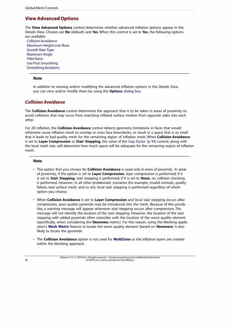
8/10/2019 ANSYS Meshing Users Guide
http://slidepdf.com/reader/full/ansys-meshing-users-guide 98/491
View Advanced Options
The View Advanced Options control determines whether advanced inflation options appear in theDetails View. Choices are No (default) and Yes. When this control is set to Yes, the following optionsare available:
Collision AvoidanceMaximum Height over Base
Growth Rate TypeMaximum AngleFillet RatioUse Post SmoothingSmoothing Iterations
Note
In addition to viewing and/or modifying the advanced inflation options in the Details View,you can view and/or modify them by using the Options dialog box.
Collision Avoidance The Collision Avoidance control determines the approach that is to be taken in areas of proximity toavoid collisions that may occur from marching inflated surface meshes from opposite sides into each
other.
For 2D inflation, the Collision Avoidance control detects geometry limitations in faces that wouldotherwise cause inflation mesh to overlap or cross face boundaries, or result in a space that is so smallthat it leads to bad quality mesh for the remaining region of inflation mesh. When Collision Avoidance
is set to Layer Compression or Stair Stepping, the value of the Gap Factor (p. 94) control, along withthe local mesh size, will determine how much space will be adequate for the remaining region of inflationmesh.
Note
• The option that you choose for Collision Avoidance is used only in areas of proximity . In areasof proximity, if the option is set to Layer Compression, layer compression is performed; if itis set to Stair Stepping, stair stepping is performed; if it is set to None, no collision checkingis performed. However, in all other problematic scenarios (for example, invalid normals, quality
failure, bad surface mesh, and so on), local stair stepping is performed regardless of whichoption you choose.
• When Collision Avoidance is set to Layer Compression and local stair stepping occurs after
compression, poor quality pyramids may be introduced into the mesh. Because of this possib-ility, a warning message will appear whenever stair stepping occurs after compression. Themessage will not identify the location of the stair stepping. However, the location of the stairstepping with added pyramids often coincides with the location of the worst quality element
(specifically, when considering the Skewness metric). For this reason, using the Meshing applic-ation's Mesh Metric feature to locate the worst quality element (based on Skewness) is alsolikely to locate the pyramids.
• The Collision Avoidance option is not used for MultiZone as the inflation layers are createdwithin the blocking approach.
Release 15.0 - © SAS IP, Inc. All rights reserved. - Contains proprietary and confidential informationof ANSYS, Inc. and its subsidiaries and affiliates.90
Global Mesh Controls

8/10/2019 ANSYS Meshing Users Guide
http://slidepdf.com/reader/full/ansys-meshing-users-guide 99/491
• For assembly meshing algorithms, Collision Avoidance is set to Layer Compression and isread-only. Refer to Assembly Meshing (p. 273) for details.
The following options are available:
• None - The None option does not check for layer collisions. Selecting this option speeds up inflation
layer computation time; however, it can result in an invalid mesh and mesh failures as a result. For thesereasons, this option is not recommended.
For 2D inflation, if a collision/proximity limitation is detected during layer creation, creation of inflationlayers stops with the previous layer. (Inflation stops completely ; contrast with Stair Stepping below.)
• Layer Compression - The Layer Compression option compresses inflation layers in areas of collision. In
these areas, the defined heights and ratios are reduced to ensure the same number of layers throughoutthe entire inflation region. Generally, this option is best for avoiding the creation of pyramids in the mesLayer Compression is the default only when the Physics Preference is set to CFD and the Solver Pref-
erence is set to Fluent; otherwise, the default is Stair Stepping.
For 2D inflation, if a collision/proximity limitation is detected during layer creation, inflation heightswill shrink locally. If Fix First Layer (p. 94) is set to Yes, the First Layer Height (p. 86) will not be scaled.
For details about the additional controls that appear when Layer Compression is selected, refer tothe descriptions of the Fix First Layer (p. 94) and Gap Factor (p. 94) controls.
• Stair Stepping - Rather than compressing the prism layers, with Stair Stepping the prism layers are “stastepped” in the proximity region to avoid collision and to maintain the gap defined by Gap Factor (p. 94
The Stair Stepping approach to inflation growth locally reduces inflation layers to avoid collisions, as weas bad quality elements in sharp or tight corners. The term “stair stepping” refers to the steps createdbetween one layer and the next. Using this approach, special logic is used to fill the steps with pyramid
and tetrahedron elements for prism steps, or prism, pyramid, and tetrahedron elements for hex steps.
This special logic helps the mesher obtain a high-quality transition to the tetrahedral mesh. Stair Steppis the default, unless the Physics Preference is set to CFD and the Solver Preference is set to Fluent, inwhich case the default is Layer Compression.
For 2D inflation, if a collision/proximity limitation is detected during layer creation, creation of inflationlayers stops locally . (Contrast with None above.)
An additional control, for Gap Factor, appears when Stair Stepping is selected.
The figures below illustrate how the Layer Compression and Stair Stepping options differ.
9Release 15.0 - © SAS IP, Inc. All rights reserved. - Contains proprietary and confidential informationof ANSYS, Inc. and its subsidiaries and affiliates.
Inflation Group
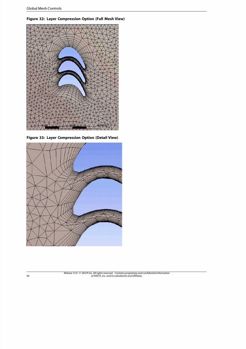
8/10/2019 ANSYS Meshing Users Guide
http://slidepdf.com/reader/full/ansys-meshing-users-guide 100/491
Figure 32: Layer Compression Option (Full Mesh View)
Figure 33: Layer Compression Option (Detail View)
Release 15.0 - © SAS IP, Inc. All rights reserved. - Contains proprietary and confidential informationof ANSYS, Inc. and its subsidiaries and affiliates.92
Global Mesh Controls
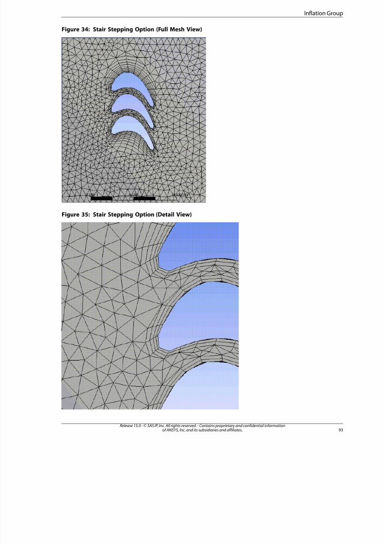
8/10/2019 ANSYS Meshing Users Guide
http://slidepdf.com/reader/full/ansys-meshing-users-guide 101/491
Figure 34: Stair Stepping Option (Full Mesh View)
Figure 35: Stair Stepping Option (Detail View)
93Release 15.0 - © SAS IP, Inc. All rights reserved. - Contains proprietary and confidential informationof ANSYS, Inc. and its subsidiaries and affiliates.
Inflation Group
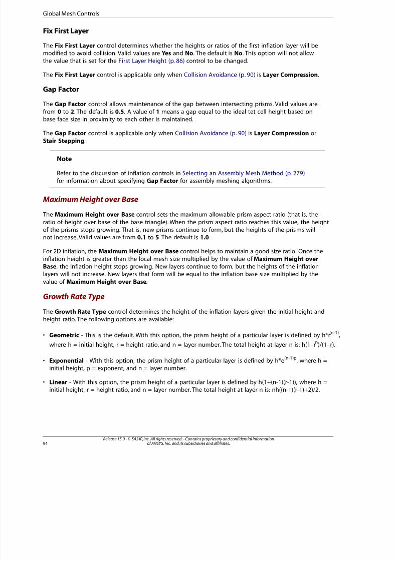
8/10/2019 ANSYS Meshing Users Guide
http://slidepdf.com/reader/full/ansys-meshing-users-guide 102/491
Fix First Layer
The Fix First Layer control determines whether the heights or ratios of the first inflation layer will bemodified to avoid collision. Valid values are Yes and No. The default is No. This option will not allow
the value that is set for the First Layer Height (p. 86) control to be changed.
The Fix First Layer control is applicable only when Collision Avoidance (p. 90) is Layer Compression.
Gap Factor
The Gap Factor control allows maintenance of the gap between intersecting prisms. Valid values are
from 0 to 2. The default is 0.5. A value of 1 means a gap equal to the ideal tet cell height based onbase face size in proximity to each other is maintained.
The Gap Factor control is applicable only when Collision Avoidance (p. 90) is Layer Compression or
Stair Stepping.
Note
Refer to the discussion of inflation controls in Selecting an Assembly Mesh Method (p. 279)for information about specifying Gap Factor for assembly meshing algorithms.
Maximum Height over Base
The Maximum Height over Base control sets the maximum allowable prism aspect ratio (that is, the
ratio of height over base of the base triangle). When the prism aspect ratio reaches this value, the heightof the prisms stops growing. That is, new prisms continue to form, but the heights of the prisms willnot increase. Valid values are from 0.1 to 5. The default is 1.0.
For 2D inflation, the Maximum Height over Base control helps to maintain a good size ratio. Once the
inflation height is greater than the local mesh size multiplied by the value of Maximum Height over
Base, the inflation height stops growing. New layers continue to form, but the heights of the inflationlayers will not increase. New layers that form will be equal to the inflation base size multiplied by the
value of Maximum Height over Base.
Growth Rate Type
The Growth Rate Type control determines the height of the inflation layers given the initial height andheight ratio. The following options are available:
• Geometric - This is the default. With this option, the prism height of a particular layer is defined by h*r(n-1)
,
where h = initial height, r = height ratio, and n = layer number. The total height at layer n is: h(1–rn)/(1–r).
• Exponential - With this option, the prism height of a particular layer is defined by h*e(n-1)p
, where h =initial height, p = exponent, and n = layer number.
• Linear - With this option, the prism height of a particular layer is defined by h(1+(n-1)(r-1)), where h =initial height, r = height ratio, and n = layer number. The total height at layer n is: nh((n-1)(r-1)+2)/2.
Release 15.0 - © SAS IP, Inc. All rights reserved. - Contains proprietary and confidential informationof ANSYS, Inc. and its subsidiaries and affiliates.94
Global Mesh Controls
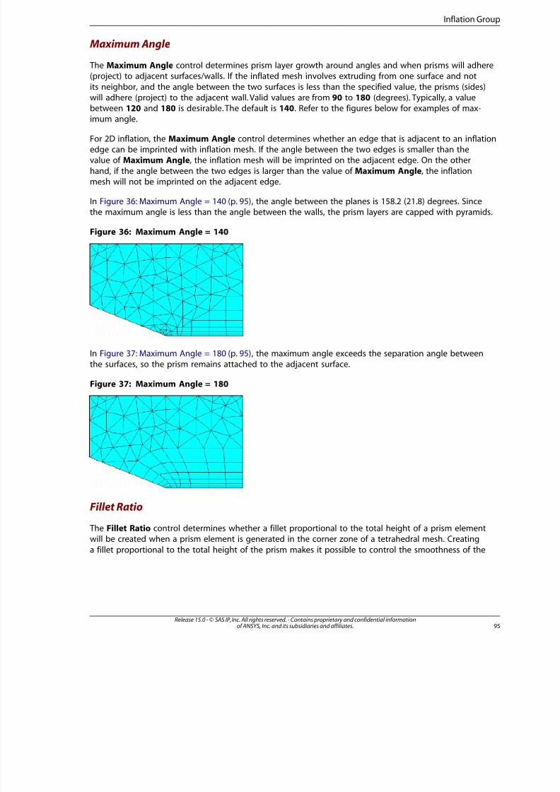
8/10/2019 ANSYS Meshing Users Guide
http://slidepdf.com/reader/full/ansys-meshing-users-guide 103/491
Maximum Angle
The Maximum Angle control determines prism layer growth around angles and when prisms will adhere(project) to adjacent surfaces/walls. If the inflated mesh involves extruding from one surface and not
its neighbor, and the angle between the two surfaces is less than the specified value, the prisms (sides)will adhere (project) to the adjacent wall. Valid values are from 90 to 180 (degrees). Typically, a valuebetween 120 and 180 is desirable. The default is 140. Refer to the figures below for examples of max-imum angle.
For 2D inflation, the Maximum Angle control determines whether an edge that is adjacent to an inflationedge can be imprinted with inflation mesh. If the angle between the two edges is smaller than thevalue of Maximum Angle, the inflation mesh will be imprinted on the adjacent edge. On the other
hand, if the angle between the two edges is larger than the value of Maximum Angle, the inflationmesh will not be imprinted on the adjacent edge.
In Figure 36: Maximum Angle = 140 (p. 95), the angle between the planes is 158.2 (21.8) degrees. Sincethe maximum angle is less than the angle between the walls, the prism layers are capped with pyramids.
Figure 36: Maximum Angle = 140
In Figure 37: Maximum Angle = 180 (p. 95), the maximum angle exceeds the separation angle betweenthe surfaces, so the prism remains attached to the adjacent surface.
Figure 37: Maximum Angle = 180
Fillet Ratio
The Fillet Ratio control determines whether a fillet proportional to the total height of a prism elementwill be created when a prism element is generated in the corner zone of a tetrahedral mesh. Creating
a fillet proportional to the total height of the prism makes it possible to control the smoothness of the
95Release 15.0 - © SAS IP, Inc. All rights reserved. - Contains proprietary and confidential informationof ANSYS, Inc. and its subsidiaries and affiliates.
Inflation Group
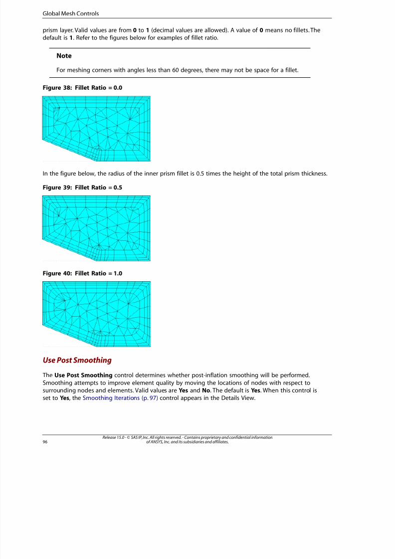
8/10/2019 ANSYS Meshing Users Guide
http://slidepdf.com/reader/full/ansys-meshing-users-guide 104/491
8/10/2019 ANSYS Meshing Users Guide
http://slidepdf.com/reader/full/ansys-meshing-users-guide 105/491
8/10/2019 ANSYS Meshing Users Guide
http://slidepdf.com/reader/full/ansys-meshing-users-guide 106/491
• CutCell - Selects the CutCell strategy for assembly meshing. Exposes assembly meshing controls andhides controls that are not applicable to assembly meshing. The CutCell option is supported only in
the Meshing application. See also Assembly Meshing (p. 273).
Note
If CutCell is active in a Mesh system and you replace the Mesh system with a Mech-
anical Model system, you will not be able to use CutCell in the Mechanical Modelsystem.
• Tetrahedrons - Selects the Tetrahedrons strategy for assembly meshing. Exposes assembly meshingcontrols and hides controls that are not applicable to assembly meshing. The Tetrahedrons optionis available and supported in the Meshing application. Tetrahedrons is also available in the Mechan-
ical application; however, meshes generated using assembly meshing are not supported for Mechan-ical solvers. If you try to use a Mechanical solver to solve an analysis of an assembly mesh, the solutionis blocked and an error message is issued. To proceed using a Mechanical solver, you must first deac-
tivate assembly meshing (set Method to None) and then regenerate the mesh. See also AssemblyMeshing (p. 273).
Note
Changing the Method control from None to Tetrahedrons while using assembly meshingto mesh an entire model may result in differing named selection titles in the system file. If
so, the new mesh will be incompatible with the Polyflow data file.
Feature Capture
The Feature Capture control determines which CAD features are captured for assembly meshing. Thefollowing options are available:
• Program Controlled - This is the default. A feature angle of 40 degrees is used to determine whichfeatures are captured. If the shared faces on an edge form an angle smaller than (180 - 40) degrees,
the edge is selected for assembly meshing.
• Feature Angle - Exposes an additional Feature Angle field, where you can set a value from 0 to 90degrees instead of using the default of 40. The smaller the angle, the higher the number of features
that are captured. If you specify a value greater than 90, a feature angle of 90 is used. Setting anegative value resets the feature angle to its default, while setting the value to 0 captures all features.
Tessellation Refinement
The Tessellation Refinement control specifies the value to be used for tessellation (faceting) refinementfor assembly meshing. The following options are available:
• Program Controlled - This is the default. Sets tessellation refinement to 10% of the value of MinSize (p. 74) /Proximity Min Size (p. 75) (whichever is smaller). This is the recommended value for mostassembly meshing operations.
• Absolute Tolerance - Exposes an additional Absolute Tolerance field, where you can set a numer-
ical value for refinement. The recommended range is between 5 and 10% of the value of Min
Release 15.0 - © SAS IP, Inc. All rights reserved. - Contains proprietary and confidential informationof ANSYS, Inc. and its subsidiaries and affiliates.98
Global Mesh Controls
8/10/2019 ANSYS Meshing Users Guide
http://slidepdf.com/reader/full/ansys-meshing-users-guide 107/491
Size (p. 74) /Proximity Min Size (p. 75) (whichever is smaller). A value on the lower end of the rangemay work better if you have problems with gaps.
• None - Sets tessellation refinement to the CAD program or DesignModeler application default setting.
Note
• To assist you in working with assembly meshing, you may want to use the Show MissingTessellations feature prior to mesh generation.
• Also see Avoiding Bad Feature Capturing in Assembly Meshing (p. 400).
Intersection Feature Creation
In cases where two parts/bodies overlap in space, the Intersection Feature Creation control determineswhether the intersection between faces is computed. When activated, Intersection Feature Creationcomputes additional feature edges to be respected during the snapping that occurs within Assembly
Meshing. Activating this feature is very useful for avoiding zigzag boundaries at an intersection, because
it ensures that the “real” intersection lines are respected. However, this operation can be computationallyexpensive, so you should de-activate it if you have many non-intersecting bodies in the model. Thefollowing options are available:
• Program Controlled — This is the default, which activates this feature whenever you have assemblies(intersecting or not intersecting).
• No — Deactivates the feature.
• Yes — Activates the feature.
Morphing Frequency
In the CutCell inflation algorithm, inflation layers are grown into the CutCell mesh. The volume meshis morphed so the boundary of the CutCell mesh matches the cap of the inflation. The value set forthe Morphing Frequency determines how often the morphing is repeated. For example, if the
Morphing Frequency is set to 5 (the default) and more than five layers are grown, then morphing isrepeated at every five layers. Similarly, if the Morphing Frequency is set to 3 and more than threelayers are grown, then morphing is repeated at every three layers.
Note
Morphing Frequency is applicable only to CutCell meshing with inflation.
Keep Solid Mesh
The Keep Solid Mesh control determines whether the mesh for any body marked as a solid is discarded
or kept. A body may be marked as a solid based on the definition of a solid that the Meshing applicationuses for exporting the assembly mesh to the solver. The following options are available:
• No - This is the default. All solid mesh is discarded. Bodies whose mesh is discarded remain in ameshed state.
99Release 15.0 - © SAS IP, Inc. All rights reserved. - Contains proprietary and confidential informationof ANSYS, Inc. and its subsidiaries and affiliates.
Assembly Meshing Group of Controls
8/10/2019 ANSYS Meshing Users Guide
http://slidepdf.com/reader/full/ansys-meshing-users-guide 108/491
• Yes - All solid mesh is kept.
Note
The Keep Solid Mesh control does not appear until a virtual body has been created.
Patch Conforming Options Group
The Patch Conforming Options group allows you to control these options:
Triangle Surface Mesher
The Patch Conforming Options group of controls is inaccessible when an assembly meshing algorithmis selected.
Triangle Surface Mesher
The Triangle Surface Mesher control determines which triangle surface meshing strategy will be usedby patch conforming meshers. In general, the advancing front algorithm provides a smoother size
variation and better results for skewness and orthogonal quality. The following options are available:
• Program Controlled - This is the default. The mesher determines whether to use the Delaunay or advancingfront algorithm based on a variety of factors such as surface type, face topology, and defeatured bound-
aries.
• Advancing Front - The mesher uses advancing front as its primary algorithm, but falls back to Delaunayif problems occur.
Note
If the mesher falls back to Delaunay, the edge mesh from the advancing front algorithm
could still be used and in some rare cases could lead to meshing failures. Switching to theProgram Controlled option could fix the issue as the starting edge mesh could be better.
The figures below illustrate the difference between the Program Controlled and Advancing Front
options.
Release 15.0 - © SAS IP, Inc. All rights reserved. - Contains proprietary and confidential informationof ANSYS, Inc. and its subsidiaries and affiliates.100
Global Mesh Controls
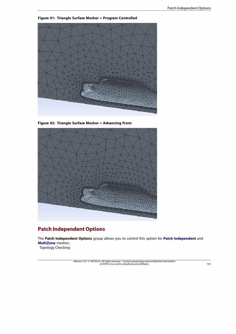
8/10/2019 ANSYS Meshing Users Guide
http://slidepdf.com/reader/full/ansys-meshing-users-guide 109/491
Figure 41: Triangle Surface Mesher = Program Controlled
Figure 42: Triangle Surface Mesher = Advancing Front
Patch Independent Options
The Patch Independent Options group allows you to control this option for Patch Independent andMultiZone meshes:
Topology Checking
10Release 15.0 - © SAS IP, Inc. All rights reserved. - Contains proprietary and confidential informationof ANSYS, Inc. and its subsidiaries and affiliates.
Patch Independent Options

8/10/2019 ANSYS Meshing Users Guide
http://slidepdf.com/reader/full/ansys-meshing-users-guide 110/491
Topology Checking
The Topology Checking option determines whether the mesher performs topology checks for PatchIndependent and MultiZone meshes. If set to No, the mesher skips topology checks except where itis necessary to imprint all protected topologies. You will then need to independently validate the topology
and that boundary conditions are properly applied to the mesh. The default is Yes, in which case themesher performs all topology checks.
Patch Independent meshing is dependent on loads, boundary conditions, Named Selections, results
or any scoped object. If Topology Checking is on, you should define all of your scoping dependenciesbefore meshing. If you change a scoping after meshing, you may need to re-mesh. If Topology Checkingis off, you will be able to scope new objects and the mesh will not go out of date, but you should val-idate that the new objects created have mesh associated to them to be sure loads, boundary conditions,
Named Selections, etc., will transfer properly to the simulation. You can check this by plotting the meshon Named Selections. For more information about Patch Independent meshing, see Patch Independ-ent (p. 3).
Note
The Topology Checking option does not support Assembly meshing.
If you use MultiZone mesh method and set Preserve Boundaries to All, the MultiZone meshmethod behaves in a patch conforming way, and topology checks are skipped independentof whether this option is set to Yes or No.
If you use the Use MultiZone for Sweepable Bodies option, the MultiZone mesh methodbehaves in a more patch conforming way, and topology checks are skipped independent of whether this option is set to Yes or No.
The following figure shows a case where Topology Checking is on and the meshing fails because acontact region does not have a properly associated mesh. If Topology Checking is turned off for thismodel, the mesh will not fail and you can validate the mesh manually.
Release 15.0 - © SAS IP, Inc. All rights reserved. - Contains proprietary and confidential informationof ANSYS, Inc. and its subsidiaries and affiliates.102
Global Mesh Controls
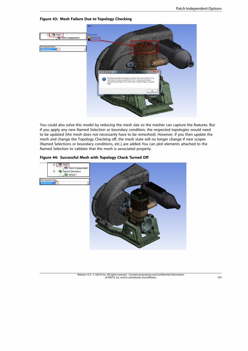
8/10/2019 ANSYS Meshing Users Guide
http://slidepdf.com/reader/full/ansys-meshing-users-guide 111/491
Figure 43: Mesh Failure Due to Topology Checking
You could also solve this model by reducing the mesh size so the mesher can capture the features. But
if you apply any new Named Selection or boundary condition, the respected topologies would needto be updated (the mesh does not necessarily have to be remeshed). However, if you then update themesh and change the Topology Checking off, the mesh state will no longer change if new scopes(Named Selections or boundary conditions, etc.), are added. You can plot elements attached to the
Named Selection to validate that the mesh is associated properly.
Figure 44: Successful Mesh with Topology Check Turned Off
103Release 15.0 - © SAS IP, Inc. All rights reserved. - Contains proprietary and confidential informationof ANSYS, Inc. and its subsidiaries and affiliates.
Patch Independent Options
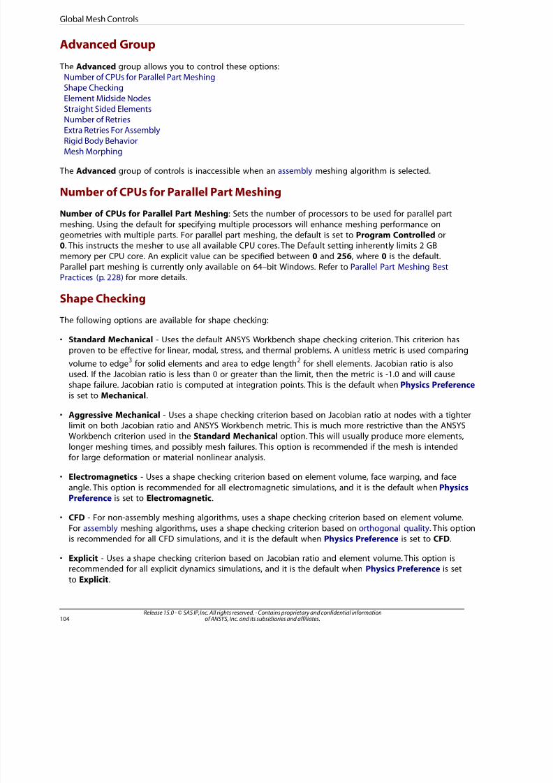
8/10/2019 ANSYS Meshing Users Guide
http://slidepdf.com/reader/full/ansys-meshing-users-guide 112/491
Advanced Group
The Advanced group allows you to control these options:Number of CPUs for Parallel Part MeshingShape Checking
Element Midside NodesStraight Sided Elements
Number of RetriesExtra Retries For Assembly
Rigid Body BehaviorMesh Morphing
The Advanced group of controls is inaccessible when an assembly meshing algorithm is selected.
Number of CPUs for Parallel Part Meshing
Number of CPUs for Parallel Part Meshing : Sets the number of processors to be used for parallel part
meshing. Using the default for specifying multiple processors will enhance meshing performance ongeometries with multiple parts. For parallel part meshing, the default is set to Program Controlled or
0. This instructs the mesher to use all available CPU cores. The Default setting inherently limits 2 GBmemory per CPU core. An explicit value can be specified between 0 and 256, where 0 is the default.
Parallel part meshing is currently only available on 64–bit Windows. Refer to Parallel Part Meshing BestPractices (p. 228) for more details.
Shape Checking
The following options are available for shape checking:
• Standard Mechanical - Uses the default ANSYS Workbench shape checking criterion. This criterion has
proven to be effective for linear, modal, stress, and thermal problems. A unitless metric is used comparing
volume to edge3 for solid elements and area to edge length
2 for shell elements. Jacobian ratio is also
used. If the Jacobian ratio is less than 0 or greater than the limit, then the metric is -1.0 and will causeshape failure. Jacobian ratio is computed at integration points. This is the default when Physics Preference
is set to Mechanical.
• Aggressive Mechanical - Uses a shape checking criterion based on Jacobian ratio at nodes with a tighterlimit on both Jacobian ratio and ANSYS Workbench metric. This is much more restrictive than the ANSYSWorkbench criterion used in the Standard Mechanical option. This will usually produce more elements,
longer meshing times, and possibly mesh failures. This option is recommended if the mesh is intendedfor large deformation or material nonlinear analysis.
• Electromagnetics - Uses a shape checking criterion based on element volume, face warping, and face
angle. This option is recommended for all electromagnetic simulations, and it is the default when PhysicsPreference is set to Electromagnetic.
• CFD - For non-assembly meshing algorithms, uses a shape checking criterion based on element volume.
For assembly meshing algorithms, uses a shape checking criterion based on orthogonal quality. This optionis recommended for all CFD simulations, and it is the default when Physics Preference is set to CFD.
• Explicit - Uses a shape checking criterion based on Jacobian ratio and element volume. This option isrecommended for all explicit dynamics simulations, and it is the default when Physics Preference is set
to Explicit.
Release 15.0 - © SAS IP, Inc. All rights reserved. - Contains proprietary and confidential informationof ANSYS, Inc. and its subsidiaries and affiliates.104
Global Mesh Controls
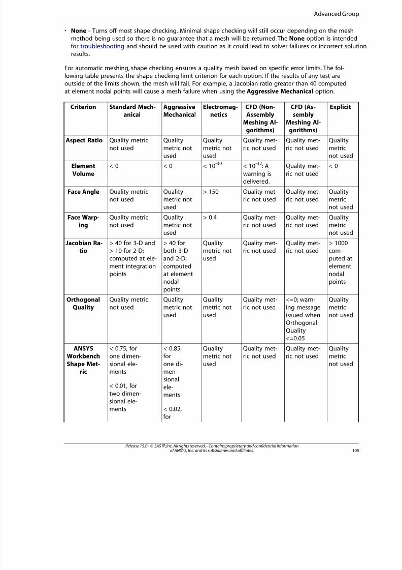
8/10/2019 ANSYS Meshing Users Guide
http://slidepdf.com/reader/full/ansys-meshing-users-guide 113/491
• None - Turns off most shape checking. Minimal shape checking will still occur depending on the meshmethod being used so there is no guarantee that a mesh will be returned. The None option is intended
for troubleshooting and should be used with caution as it could lead to solver failures or incorrect solutresults.
For automatic meshing, shape checking ensures a quality mesh based on specific error limits. The fol-
lowing table presents the shape checking limit criterion for each option. If the results of any test areoutside of the limits shown, the mesh will fail. For example, a Jacobian ratio greater than 40 computed
at element nodal points will cause a mesh failure when using the Aggressive Mechanical option.
ExplicitCFD (As-sembly
Meshing Al-
gorithms)
CFD (Non-Assembly
Meshing Al-
gorithms)
Electromag-netics
AggressiveMechanical
Standard Mech-anical
Criterion
Quality
metricnot used
Quality met-
ric not used
Quality met-
ric not used
Quality
metric notused
Quality
metric notused
Quality metric
not used
Aspect Ratio
< 0Quality met-
ric not used
< 10-32
: A
warning is
delivered.
< 10-30
< 0< 0Element
Volume
Qualitymetricnot used
Quality met-ric not used
Quality met-ric not used
> 150Qualitymetric notused
Quality metricnot used
Face Angle
Qualitymetricnot used
Quality met-ric not used
Quality met-ric not used
> 0.4Qualitymetric notused
Quality metricnot used
Face Warp-ing
> 1000com-
Quality met-ric not used
Quality met-ric not used
Qualitymetric notused
> 40 forboth 3-Dand 2-D;
> 40 for 3-D and> 10 for 2-D;computed at ele-
Jacobian Ra-tio
puted at
computedment integrationpoints elementnodalpoints
at elementnodal
points
Qualitymetric
not used
<=0; warn-ing message
issued when
Quality met-ric not used
Qualitymetric not
used
Qualitymetric not
used
Quality metricnot used
OrthogonalQuality
OrthogonalQuality
<=0.05
Quality
metricnot used
Quality met-
ric not used
Quality met-
ric not used
Quality
metric notused
< 0.85,
forone di-
< 0.75, for
one dimen-sional ele-ments
ANSYS
WorkbenchShape Met-
ric men-
< 0.01, for
two dimen-
sional
ele-ments
sional ele-ments < 0.02,
for
105Release 15.0 - © SAS IP, Inc. All rights reserved. - Contains proprietary and confidential informationof ANSYS, Inc. and its subsidiaries and affiliates.
Advanced Group
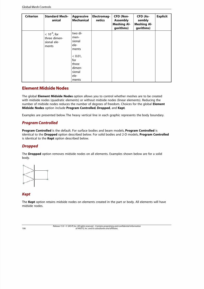
8/10/2019 ANSYS Meshing Users Guide
http://slidepdf.com/reader/full/ansys-meshing-users-guide 114/491
ExplicitCFD (As-sembly
Meshing Al-gorithms)
CFD (Non-Assembly
Meshing Al-gorithms)
Electromag-netics
AggressiveMechanical
Standard Mech-anical
Criterion
< 10-4
, forthree dimen-
two di-men-
sionalsional ele-
ments ele-ments
< 0.01,
forthreedimen-
sionalele-ments
Element Midside Nodes
The global Element Midside Nodes option allows you to control whether meshes are to be createdwith midside nodes (quadratic elements) or without midside nodes (linear elements). Reducing thenumber of midside nodes reduces the number of degrees of freedom. Choices for the global ElementMidside Nodes option include Program Controlled, Dropped, and Kept.
Examples are presented below. The heavy vertical line in each graphic represents the body boundary.
Program Controlled
Program Controlled is the default. For surface bodies and beam models, Program Controlled is
identical to the Dropped option described below. For solid bodies and 2-D models, Program Controlledis identical to the Kept option described below.
Dropped
The Dropped option removes midside nodes on all elements. Examples shown below are for a solidbody.
Kept
The Kept option retains midside nodes on elements created in the part or body. All elements will have
midside nodes.
Release 15.0 - © SAS IP, Inc. All rights reserved. - Contains proprietary and confidential informationof ANSYS, Inc. and its subsidiaries and affiliates.106
Global Mesh Controls
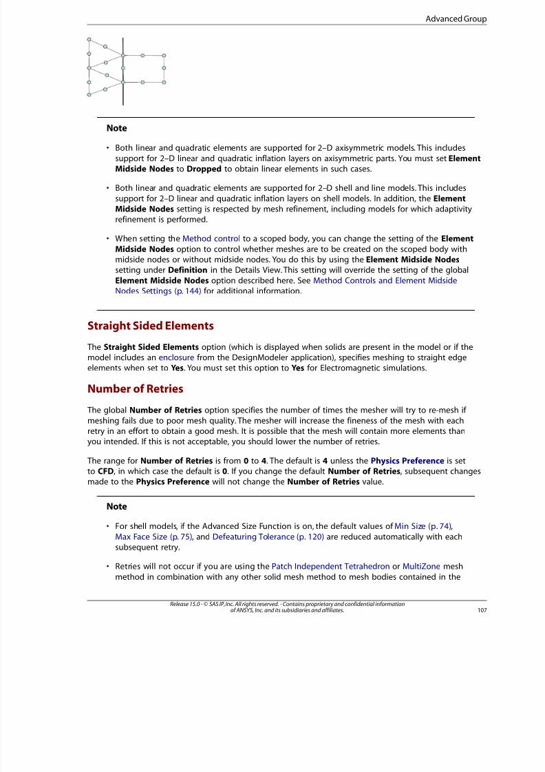
8/10/2019 ANSYS Meshing Users Guide
http://slidepdf.com/reader/full/ansys-meshing-users-guide 115/491
Note
• Both linear and quadratic elements are supported for 2–D axisymmetric models. This includes
support for 2–D linear and quadratic inflation layers on axisymmetric parts. You must set ElementMidside Nodes to Dropped to obtain linear elements in such cases.
• Both linear and quadratic elements are supported for 2–D shell and line models. This includes
support for 2–D linear and quadratic inflation layers on shell models. In addition, the ElementMidside Nodes setting is respected by mesh refinement, including models for which adaptivityrefinement is performed.
• When setting the Method control to a scoped body, you can change the setting of the ElementMidside Nodes option to control whether meshes are to be created on the scoped body withmidside nodes or without midside nodes. You do this by using the Element Midside Nodessetting under Definition in the Details View. This setting will override the setting of the global
Element Midside Nodes option described here. See Method Controls and Element MidsideNodes Settings (p. 144) for additional information.
Straight Sided Elements
The Straight Sided Elements option (which is displayed when solids are present in the model or if themodel includes an enclosure from the DesignModeler application), specifies meshing to straight edgeelements when set to Yes. You must set this option to Yes for Electromagnetic simulations.
Number of Retries
The global Number of Retries option specifies the number of times the mesher will try to re-mesh if
meshing fails due to poor mesh quality. The mesher will increase the fineness of the mesh with eachretry in an effort to obtain a good mesh. It is possible that the mesh will contain more elements thanyou intended. If this is not acceptable, you should lower the number of retries.
The range for Number of Retries is from 0 to 4. The default is 4 unless the Physics Preference is setto CFD, in which case the default is 0. If you change the default Number of Retries, subsequent changes
made to the Physics Preference will not change the Number of Retries value.
Note
• For shell models, if the Advanced Size Function is on, the default values of Min Size (p. 74),
Max Face Size (p. 75), and Defeaturing Tolerance (p. 120) are reduced automatically with eachsubsequent retry.
• Retries will not occur if you are using the Patch Independent Tetrahedron or MultiZone mesh
method in combination with any other solid mesh method to mesh bodies contained in the
107Release 15.0 - © SAS IP, Inc. All rights reserved. - Contains proprietary and confidential informationof ANSYS, Inc. and its subsidiaries and affiliates.
Advanced Group

8/10/2019 ANSYS Meshing Users Guide
http://slidepdf.com/reader/full/ansys-meshing-users-guide 116/491
same part, or if you are using MultiZone Quad/Tri in combination with any other surface meshmethod to mesh bodies contained in the same part. Moreover, if a single body in a multibody
part fails during selective meshing, the mesher returns as much of the mesh as possible.
• If Number of Retries is set to 0 and a single body in a multibody part fails during selectivemeshing, the mesher returns as much of the mesh as possible. Bodies with valid meshes will
have a meshed state while bodies with invalid or partial meshes will have an unmeshed state.
You can display and examine the partially meshed bodies and then apply more mesh controlsto correct any problems you find. If Number of Retries is set to a value greater than 0 andany body fails to mesh, the mesher returns nothing for the given part. If the mesh fails after
all retries, the mesher returns nothing. The return of a partial mesh is applicable to the QuadDominant, All Triangles, MultiZone Quad/Tri, Patch Independent Tetra, and MultiZone methodsonly. The Patch Conforming Tetra, Sweep (general or thin), and Hex Dominant methods cannotreturn partial meshes.
• If you are performing selective meshing and at least one body of a particular part has beenmeshed successfully, no additional retries will occur if the mesh of a subsequent body withinthat same part fails.
• The Number of Retries option is also available in the Options dialog box, which you can accessby selecting Tools> Options from the main menu. Setting the global Number of Retries optionto -1 reads the value set on the Options dialog box and uses it as the default number of retries.
Extra Retries For Assembly
The Extra Retries For Assembly option specifies whether the mesher should perform extra retries
when meshing an assembly if meshing would otherwise fail due to poor mesh quality. The default isYes. These retries are in addition to the number specified by the Number of Retries option. Themesher will increase the fineness of the mesh with each additional retry in an effort to obtain a good
mesh. If this is not acceptable, you should set the option to No.
This control is also available in the Options dialog box, which you can access by selecting Tools> Optionsfrom the main menu.
Rigid Body Behavior
The Rigid Body Behavior option determines whether a full mesh is generated for a rigid body, ratherthan a surface contact mesh. Rigid Body Behavior is applicable to all body types. Valid values for Rigid
Body Behavior are Dimensionally Reduced (generate surface contact mesh only) and Full Mesh(generate full mesh). The default is Dimensionally Reduced unless the Physics Preference is set toExplicit. For more information, refer to Rigid Body Meshing (p. 324).
Mesh Morphing
When the Mesh Morphing feature is Enabled, you can specify that a morphed mesh is produced fol-lowing a geometry change rather than re-meshing the geometry.
For this feature to operate properly, you cannot make any topological changes when you modify/deformthe geometry. In other words, the deformed geometry must have the same number of parts, bodies,faces, edges, and/or vertices as your original geometry and also the same connectivity between these
geometric entities. The Mesh Morphing feature updates changes in nodes' coordinates, but it is not
Release 15.0 - © SAS IP, Inc. All rights reserved. - Contains proprietary and confidential informationof ANSYS, Inc. and its subsidiaries and affiliates.108
Global Mesh Controls
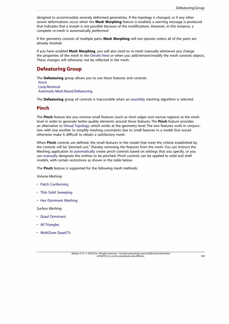
8/10/2019 ANSYS Meshing Users Guide
http://slidepdf.com/reader/full/ansys-meshing-users-guide 117/491
designed to accommodate severely deformed geometries. If the topology is changed, or if any othersevere deformations occur when the Mesh Morphing feature is enabled, a warning message is produced
that indicates that a morph is not possible because of the modifications. However, in this instance, acomplete re-mesh is automatically performed.
If the geometry consists of multiple parts, Mesh Morphing will not operate unless all of the parts are
already meshed.
If you have enabled Mesh Morphing, you will also need to re-mesh manually whenever you changethe properties of the mesh in the Details View or when you add/remove/modify the mesh controls objects
These changes will otherwise not be reflected in the mesh.
Defeaturing Group
The Defeaturing group allows you to use these features and controls:
PinchLoop RemovalAutomatic Mesh Based Defeaturing
The Defeaturing group of controls is inaccessible when an assembly meshing algorithm is selected.
Pinch
The Pinch feature lets you remove small features (such as short edges and narrow regions) at the meshlevel in order to generate better quality elements around those features. The Pinch feature providesan alternative to Virtual Topology, which works at the geometry level. The two features work in conjunc-tion with one another to simplify meshing constraints due to small features in a model that would
otherwise make it difficult to obtain a satisfactory mesh.
When Pinch controls are defined, the small features in the model that meet the criteria established bythe controls will be “pinched out,” thereby removing the features from the mesh. You can instruct the
Meshing application to automatically create pinch controls based on settings that you specify, or youcan manually designate the entities to be pinched. Pinch controls can be applied to solid and shellmodels, with certain restrictions as shown in the table below.
The Pinch feature is supported for the following mesh methods:
Volume Meshing:
• Patch Conforming
• Thin Solid Sweeping
• Hex Dominant Meshing
Surface Meshing:
• Quad Dominant
• All Triangles
• MultiZone Quad/Tri
109Release 15.0 - © SAS IP, Inc. All rights reserved. - Contains proprietary and confidential informationof ANSYS, Inc. and its subsidiaries and affiliates.
Defeaturing Group

8/10/2019 ANSYS Meshing Users Guide
http://slidepdf.com/reader/full/ansys-meshing-users-guide 118/491
The table below shows the types of model (solid or shell), mesh methods, pinch creation methods (autoor manual), and pinch behaviors (pre or post) that are supported for each type of pinch control. Also
see Defining Pinch Controls Locally (p. 212) for additional restrictions on pre and post pinch behaviors.
Pinch Behavi-
or
Pinch Cre-
ation Method
Mesh MethodModel TypeEntit-
iesin
Pinch
Con-trol:Mas-ter >
Slave
PostPre
Manu-
alPinch
AutoPinch
Mul-tiZoneQuad/ Tri
AllTri
QuadDom-
in-ant
HexDom-
in-ant
ThinSolidSweep-ing
PatchCon-form-ing
ShellSolid
XXXXXXXXXXXXEdge
>Edge
XXXXXXXXXXXEdge
>Ver-tex
XXXXXXXXXXXXVer-tex >Ver-
tex
XXXXXXFace
>Edge
XXXXXXXFace
>
Ver-tex
Examples of a Mesh With and Without Pinch
The figures below illustrate the effect of pinch controls on the mesh. The first figure shows where thepinch controls have been defined in the model. The second and third figures show the meshes thatare generated without the pinch controls and with the pinch controls, respectively.
Release 15.0 - © SAS IP, Inc. All rights reserved. - Contains proprietary and confidential informationof ANSYS, Inc. and its subsidiaries and affiliates.110
Global Mesh Controls
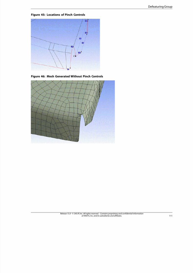
8/10/2019 ANSYS Meshing Users Guide
http://slidepdf.com/reader/full/ansys-meshing-users-guide 119/491
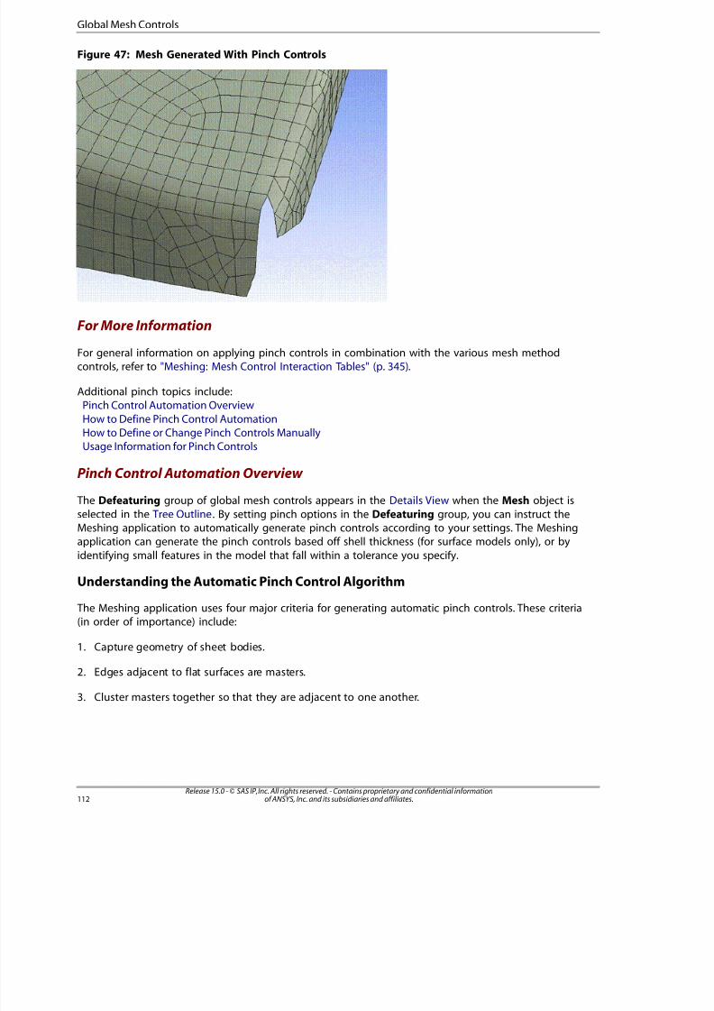
8/10/2019 ANSYS Meshing Users Guide
http://slidepdf.com/reader/full/ansys-meshing-users-guide 120/491
Figure 47: Mesh Generated With Pinch Controls
For More Information
For general information on applying pinch controls in combination with the various mesh methodcontrols, refer to "Meshing: Mesh Control Interaction Tables" (p. 345).
Additional pinch topics include:Pinch Control Automation Overview
How to Define Pinch Control AutomationHow to Define or Change Pinch Controls ManuallyUsage Information for Pinch Controls
Pinch Control Automation Overview
The Defeaturing group of global mesh controls appears in the Details View when the Mesh object is
selected in the Tree Outline. By setting pinch options in the Defeaturing group, you can instruct theMeshing application to automatically generate pinch controls according to your settings. The Meshingapplication can generate the pinch controls based off shell thickness (for surface models only), or by
identifying small features in the model that fall within a tolerance you specify.
Understanding the Automatic Pinch Control Algorithm
The Meshing application uses four major criteria for generating automatic pinch controls. These criteria(in order of importance) include:
1. Capture geometry of sheet bodies.
2. Edges adjacent to flat surfaces are masters.
3. Cluster masters together so that they are adjacent to one another.
Release 15.0 - © SAS IP, Inc. All rights reserved. - Contains proprietary and confidential informationof ANSYS, Inc. and its subsidiaries and affiliates.112
Global Mesh Controls
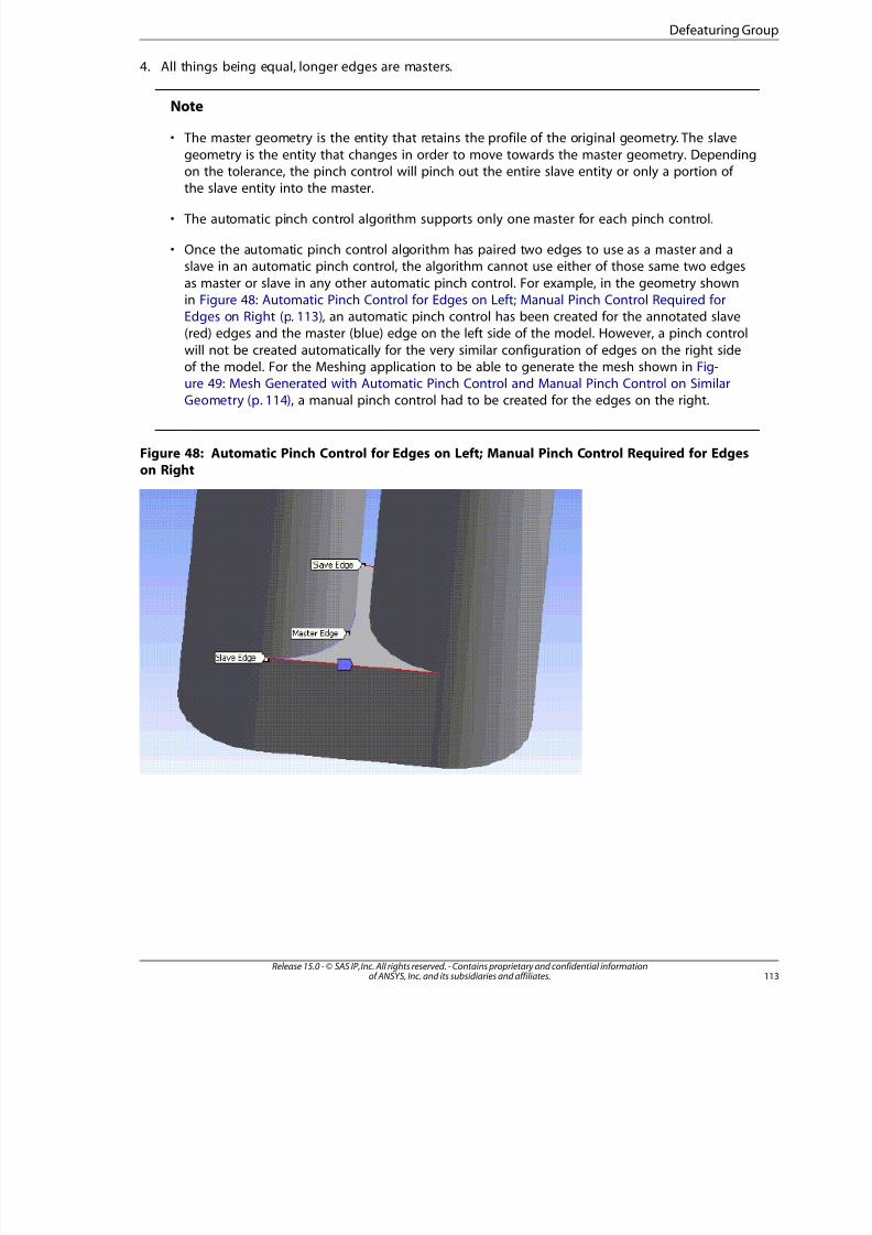
8/10/2019 ANSYS Meshing Users Guide
http://slidepdf.com/reader/full/ansys-meshing-users-guide 121/491
4. All things being equal, longer edges are masters.
Note
• The master geometry is the entity that retains the profile of the original geometry. The slave
geometry is the entity that changes in order to move towards the master geometry. Dependingon the tolerance, the pinch control will pinch out the entire slave entity or only a portion of
the slave entity into the master.
• The automatic pinch control algorithm supports only one master for each pinch control.
• Once the automatic pinch control algorithm has paired two edges to use as a master and aslave in an automatic pinch control, the algorithm cannot use either of those same two edges
as master or slave in any other automatic pinch control. For example, in the geometry shownin Figure 48: Automatic Pinch Control for Edges on Left; Manual Pinch Control Required forEdges on Right (p. 113), an automatic pinch control has been created for the annotated slave(red) edges and the master (blue) edge on the left side of the model. However, a pinch control
will not be created automatically for the very similar configuration of edges on the right sideof the model. For the Meshing application to be able to generate the mesh shown in Fig-
ure 49: Mesh Generated with Automatic Pinch Control and Manual Pinch Control on SimilarGeometry (p. 114), a manual pinch control had to be created for the edges on the right.
Figure 48: Automatic Pinch Control for Edges on Left; Manual Pinch Control Required for Edgeson Right
113Release 15.0 - © SAS IP, Inc. All rights reserved. - Contains proprietary and confidential informationof ANSYS, Inc. and its subsidiaries and affiliates.
Defeaturing Group
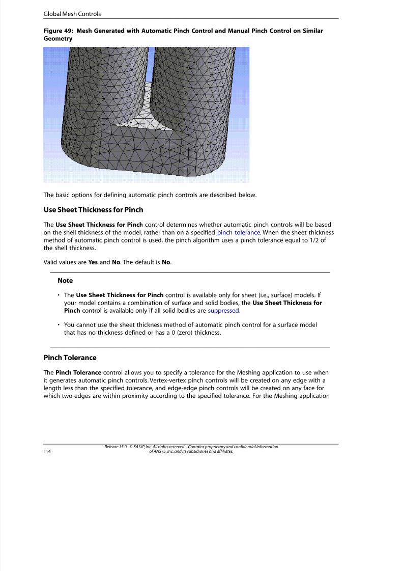
8/10/2019 ANSYS Meshing Users Guide
http://slidepdf.com/reader/full/ansys-meshing-users-guide 122/491
Figure 49: Mesh Generated with Automatic Pinch Control and Manual Pinch Control on SimilarGeometry
The basic options for defining automatic pinch controls are described below.
Use Sheet Thickness for Pinch
The Use Sheet Thickness for Pinch control determines whether automatic pinch controls will be based
on the shell thickness of the model, rather than on a specified pinch tolerance. When the sheet thicknessmethod of automatic pinch control is used, the pinch algorithm uses a pinch tolerance equal to 1/2 of the shell thickness.
Valid values are Yes and No. The default is No.
Note
• The Use Sheet Thickness for Pinch control is available only for sheet (i.e., surface) models. If your model contains a combination of surface and solid bodies, the Use Sheet Thickness forPinch control is available only if all solid bodies are suppressed.
• You cannot use the sheet thickness method of automatic pinch control for a surface modelthat has no thickness defined or has a 0 (zero) thickness.
Pinch Tolerance
The Pinch Tolerance control allows you to specify a tolerance for the Meshing application to use when
it generates automatic pinch controls. Vertex-vertex pinch controls will be created on any edge with alength less than the specified tolerance, and edge-edge pinch controls will be created on any face forwhich two edges are within proximity according to the specified tolerance. For the Meshing application
Release 15.0 - © SAS IP, Inc. All rights reserved. - Contains proprietary and confidential informationof ANSYS, Inc. and its subsidiaries and affiliates.114
Global Mesh Controls
8/10/2019 ANSYS Meshing Users Guide
http://slidepdf.com/reader/full/ansys-meshing-users-guide 123/491
to automate pinch control, you must specify a value for Pinch Tolerance unless Use Sheet Thicknessfor Pinch is set to Yes. Specify a value greater than 0.0.
Note
• The value that you specify for Pinch Tolerance should be smaller than the mesh size aroundthe region in which the pinch control is being applied. For example, if an Edge Sizing control
has been placed on an edge, a Pinch Tolerance value that is greater than that edge sizingmay cause the mesher to fail.
• In general, the value that you specify for Pinch Tolerance should be greater than the valuethat appears in the Sizing > Minimum Edge Length field. Exceptions to this guideline includemodels without seam edges, such as elliptical prism, cylinder, and sphere models.
• Do not specify an overly high value for the Pinch Tolerance control. The Pinch feature allowsthe mesher to mesh over geometry features as if they were not there, and a tolerance that isset too high can cause inverted elements.
• When the Advanced Size Function is on, the default pinch tolerance is 90% of the value of Min
Size /Proximity Min Size (whichever is smaller). This differs from the tolerance used by thedefault mesh based defeaturing; refer to Automatic Mesh Based Defeaturing (p. 120) for details.
Generate Pinch on Refresh
The Generate Pinch on Refresh control determines whether pinch controls will be regenerated followinga change made to the geometry (such as a change made via a DesignModeler application operationsuch as a merge, connect, etc.). If Generate Pinch on Refresh is set to Yes and you change the geometry,all pinch controls that were created automatically will be deleted and recreated based on the new
geometry. If Generate Pinch on Refresh is set to No and you update the geometry, all pinch controlsrelated to the changed part will appear in the Tree Outline but will be flagged as undefined.
Valid values are Yes and No. The default is No.
Note
Only Automatic pinch controls are regenerated. That is, if a pinch control has a ScopeMethod of Manual (either because it was created manually or because you made a changeto an Automatic pinch control), the pinch control will never be regenerated on refresh. SeeChanging Pinch Controls Locally (p. 215) for information about making changes to pinch
controls.
How to Define Pinch Control Automation (p. 116) provides the steps for defining automatic pinch controls.
115Release 15.0 - © SAS IP, Inc. All rights reserved. - Contains proprietary and confidential informationof ANSYS, Inc. and its subsidiaries and affiliates.
Defeaturing Group

8/10/2019 ANSYS Meshing Users Guide
http://slidepdf.com/reader/full/ansys-meshing-users-guide 124/491

8/10/2019 ANSYS Meshing Users Guide
http://slidepdf.com/reader/full/ansys-meshing-users-guide 125/491
How to Define or Change Pinch Controls Manually
As an alternative to defining pinch control automation, you can define local controls to pinch scopedentities. You can also make changes to pinch controls, regardless of whether they were created auto-
matically or manually. For details, refer to Pinch Control (p. 211) in the local mesh controls section of the Meshing help.
Usage Information for Pinch ControlsRemember the following information when using the Pinch feature:
• When pinch controls are defined, defeaturing occurs at different times depending on the setting of
PinchBehavior. When PinchBehavior is set to Pre, pinches are processed before face meshing, and wheset to Post, pinches are processed in a separate step after all meshing is complete. The Post technologyallows the pinch controls to work across parts so that a multibody part is not required.
• Post pinches are not available on solid bodies.
• The Pinch feature works on faces, edges, and vertices only; bodies cannot be pinched. Refer to the tablein Pinch (p. 109) for restrictions related to entity types.
• The automatic pinch control algorithm supports only one master for each pinch control. In manual pinccontrols, you can specify multiple faces or multiple edges to act as masters, but only one vertex can actas master.
• When defining manual pinch controls, using the same master in more than one pinch control is support
This is true for all types of manual pinch controls: edge-edge, edge-vertex, vertex-vertex, face-edge, andface-vertex. When multiple pinch controls use the same master, the aggregate of the pinch controls isused to determine the pinch. Note that this behavior differs from that of other mesh controls when mult
are specified. With other mesh controls, the control that appears lowest in the Tree is honored.
• If there are hard size constraints on a master, the pinch control will be skipped completely. If there are
hard size constraints on slaves, only the slaves with the constraints will be skipped. In either case, awarning message will be issued.
• If your model contains multibody parts and you want pinch controls to operate on selected parts/bodieonly, you must first suppress the parts/bodies that you do not want the pinch controls to apply to. Thenfollow the steps outlined in How to Define Pinch Control Automation (p. 116).
There is an alternative to this procedure if you are generating mesh connections (which involveautomatic generation of post pinch controls internally at meshing time). In the case of mesh connec-tions, you can change the settings in the Details View of the Connection Group folder so that auto-matic connection generation operates on scoped geometry only. For more information, see Common
Connections Folder Operations for Auto Generated Connections in the Mechanical help.
• If the geometry fails to mesh correctly due to the pinched features, an error message is generated. Tohighlight the geometry that is responsible for the message, select the message, right-click, and select
Show Problematic Geometry from the context menu.
• For Pre pinches only, when a face contains an internal loop with a pinch control and the edges of theloop become a “single internal edge” due to pinching, the surface mesher may completely ignore the“single” edge (that is, the surface mesher may mesh over the edge). The reason that this may occur is tha
a pinch control never changes the topology of a model. When a surface mesher collects all boundaryedge meshes before performing surface meshing, it considers the newly created “single” edge to be a
117Release 15.0 - © SAS IP, Inc. All rights reserved. - Contains proprietary and confidential informationof ANSYS, Inc. and its subsidiaries and affiliates.
Defeaturing Group
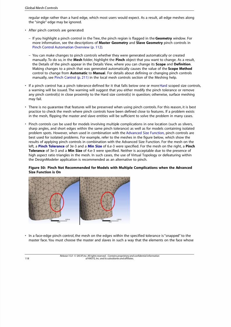
8/10/2019 ANSYS Meshing Users Guide
http://slidepdf.com/reader/full/ansys-meshing-users-guide 126/491
regular edge rather than a hard edge, which most users would expect. As a result, all edge meshes alongthe “single” edge may be ignored.
• After pinch controls are generated:
– If you highlight a pinch control in the Tree, the pinch region is flagged in the Geometry window. Formore information, see the descriptions of Master Geometry and Slave Geometry pinch controls in
Pinch Control Automation Overview (p. 112).
– You can make changes to pinch controls whether they were generated automatically or createdmanually. To do so, in the Mesh folder, highlight the Pinch object that you want to change. As a result,
the Details of the pinch appear in the Details View, where you can change its Scope and Definition.Making changes to a pinch that was generated automatically causes the value of the Scope Methodcontrol to change from Automatic to Manual. For details about defining or changing pinch controlsmanually, see Pinch Control (p. 211) in the local mesh controls section of the Meshing help.
• If a pinch control has a pinch tolerance defined for it that falls below one or more Hard scoped size controls,a warning will be issued. The warning will suggest that you either modify the pinch tolerance or removeany pinch control(s) in close proximity to the Hard size control(s) in question; otherwise, surface meshing
may fail.
• There is no guarantee that features will be preserved when using pinch controls. For this reason, it is bestpractice to check the mesh where pinch controls have been defined close to features. If a problem existsin the mesh, flipping the master and slave entities will be sufficient to solve the problem in many cases.
• Pinch controls can be used for models involving multiple complications in one location (such as slivers,sharp angles, and short edges within the same pinch tolerance) as well as for models containing isolatedproblem spots. However, when used in combination with the Advanced Size Function, pinch controls are
best used for isolated problems. For example, refer to the meshes in the figure below, which show theresults of applying pinch controls in combination with the Advanced Size Function. For the mesh on theleft, a Pinch Tolerance of 3e-3 and a Min Size of 6.e-3 were specified. For the mesh on the right, a PinchTolerance of 3e-3 and a Min Size of 4.e-3 were specified. Neither is acceptable due to the presence of
high aspect ratio triangles in the mesh. In such cases, the use of Virtual Topology or defeaturing withinthe DesignModeler application is recommended as an alternative to pinch.
Figure 50: Pinch Not Recommended for Models with Multiple Complications when the Advanced
Size Function is On
• In a face-edge pinch control, the mesh on the edges within the specified tolerance is “snapped” to the
master face. You must choose the master and slaves in such a way that the elements on the face whose
Release 15.0 - © SAS IP, Inc. All rights reserved. - Contains proprietary and confidential informationof ANSYS, Inc. and its subsidiaries and affiliates.118
Global Mesh Controls
8/10/2019 ANSYS Meshing Users Guide
http://slidepdf.com/reader/full/ansys-meshing-users-guide 127/491
edges are defined as slaves will be stretched onto the master face. If the edges would be "squashed," nopinch will be created.
• When a face pinch control and a mapped face meshing control are applied to the same face, the mesheattempts to generate a mapped mesh for the face. If the mesher cannot retain the mapped mesh patterit will generate a free mesh instead and issue a warning.
• If you apply a match control and a face-edge pinch control to the same topology, a warning is issued.
• Since Pinch objects cannot be duplicated, they cannot be used as template objects for the Object Geneator.
Loop Removal
The Defeaturing group of global mesh controls appears in the Details View when the Mesh object is
selected in the Tree Outline. The Meshing application automatically removes loops according to thecriteria you specify for the loop removal options in this group. Prior to meshing, you can use the ShowRemovable Loops feature to preview the loops that will be removed according to the current settings.
The loop removal feature is supported for the following mesh methods:
Surface Meshing:
• Quad Dominant
• All Triangles
• MultiZone Quad/Tri
Note
• The loop removal controls are passed to the MultiZone Quad/Tri method as described in Mul-
tiZone Quad/Tri Method Control (p. 178).
• If you are meshing with loop removal on (using the Quad Dominant or MultiZone Quad/Trimethod), making changes to a loop after meshing (such as adding a load on a loop) invalidatesthe mesh and you will need to re-mesh. It is recommended that you apply loads to the model
before meshing when using these controls. Refer to the discussion of protected topology andPatch Independent meshing for related information.
The options for defining loop removal are described below.
Sheet Loop Removal The Sheet Loop Removal control determines whether loops will be removed (i.e., meshed over) by the
mesher. When Sheet Loop Removal is set to Yes, the mesher removes any loop with a radius less thanor equal to the value of Loop Removal Tolerance.
Valid values are Yes and No. The default is No.
119Release 15.0 - © SAS IP, Inc. All rights reserved. - Contains proprietary and confidential informationof ANSYS, Inc. and its subsidiaries and affiliates.
Defeaturing Group
8/10/2019 ANSYS Meshing Users Guide
http://slidepdf.com/reader/full/ansys-meshing-users-guide 128/491
Loop Removal Tolerance
The Loop Removal Tolerance control sets the tolerance for loop removal. Any loop with a radius lessthan or equal to the value of Loop Removal Tolerance will be meshed over by the mesher.
Specify a value greater than 0.0.
Automatic Mesh Based Defeaturing
The Defeaturing group of global mesh controls appears in the Details View when the Mesh object isselected in the Tree Outline. The Meshing application automatically defeatures small features and dirtygeometry according to the Defeaturing Tolerance you specify here.
Automatic mesh based defeaturing is supported for the following mesh methods:
Solid Meshing:
• Patch Conforming Tetrahedron
• Patch Independent Tetrahedron
• MultiZone
• Thin Sweep
• Hex Dominant
Surface Meshing:
• Quad Dominant
• All Triangles
• MultiZone Quad/Tri
For the Patch Independent Tetrahedron, MultiZone, and MultiZone Quad/Tri methods, the Defeaturing
Tolerance you set here will be populated to the local (scoped) method controls. If you subsequentlymake changes to the local settings, the local settings will override the global Defeaturing Toleranceset here. See the descriptions of the individual methods for more information.
The options for defining automatic mesh based defeaturing are described below.
Automatic Mesh Based Defeaturing
Turns Automatic Mesh Based Defeaturing on or off. When Automatic Mesh Based Defeaturing isOn (default), features smaller than or equal to the value of Defeaturing Tolerance are removed auto-matically.
Defeaturing Tolerance
Only available when Automatic Mesh Based Defeaturing is On. Sets the global tolerance for defeaturing.
Specify a value greater than 0.0. Specifying a value of 0.0 resets the defeaturing tolerance to default.
When the Advanced Size Function is on, the default Defeaturing Tolerance differs depending onwhether sheets and/or solids are present:
Release 15.0 - © SAS IP, Inc. All rights reserved. - Contains proprietary and confidential informationof ANSYS, Inc. and its subsidiaries and affiliates.120
Global Mesh Controls
8/10/2019 ANSYS Meshing Users Guide
http://slidepdf.com/reader/full/ansys-meshing-users-guide 129/491
• For sheet models, Defeaturing Tolerance is set to 75% of the value of Min Size /Proximity Min Size(whichever is smaller).
• For solid models, Defeaturing Tolerance is set to 50% of the value of Min Size /Proximity Min Size(whichever is smaller).
• For assemblies containing both sheets and solids, the Defeaturing Tolerance used for the sheets is
75% of the value of Min Size /Proximity Min Size (whichever is smaller), and for the solids, 50%.
However, the Default value that displays in the Details View is the larger value (i.e., the value beingused for sheets).
When the Advanced Size Function is off, the default Defeaturing Tolerance is handled differently de-pending on the mesh method being used. See the descriptions of the individual methods for more in-formation.
Note
• If a user-defined value has been specified for Defeaturing Tolerance, that value will be used
for everything—sheets and solids.
• If you allow the Defeaturing Tolerance to default and you modify the mesh size by applyinglocal sizing controls (for example, local face or edge sizing), the tolerance may be modified
automatically. In such cases, a warning message is issued to notify you that the global defea-turing tolerance has been modified. To prevent this behavior, manually specify a value forDefeaturing Tolerance.
• When specifying a value for Defeaturing Tolerance, do not specify a value greater than the
value of Min Size.
• If you add a hard size that is smaller than the Min Size, you must further reduce the DefeaturingTolerance with respect to the specified hard size (essentially, the hard size becomes the new
Min Size).
Statistics Group
The Statistics group lets you view and request information about these options:
NodesElementsMesh Metric
Nodes
The Nodes option provides a read-only indication of the number of nodes in the meshed model. If the
model contains multiple parts or bodies, you can view the number of nodes in an individual part orbody by highlighting it under the Geometry object in the Tree Outline.
Elements
The Elements option provides a read-only indication of the number of elements in the meshed model.If the model contains multiple parts or bodies, you can view the number of elements in an individualpart or body by highlighting it under the Geometry object in the Tree Outline.
12Release 15.0 - © SAS IP, Inc. All rights reserved. - Contains proprietary and confidential informationof ANSYS, Inc. and its subsidiaries and affiliates.
Statistics Group

8/10/2019 ANSYS Meshing Users Guide
http://slidepdf.com/reader/full/ansys-meshing-users-guide 130/491
Mesh Metric
The Mesh Metric option allows you to view mesh metric information and thereby evaluate the meshquality. Once you have generated a mesh, you can choose to view information about any of the followingmesh metrics: Element Quality (p. 127), Aspect Ratio for triangles or quadrilaterals, Jacobian Ratio (p. 130),
Warping Factor (p. 132), Parallel Deviation (p. 135), Maximum Corner Angle (p. 135), Skewness (p. 136),and Orthogonal Quality (p. 138). Selecting None turns off mesh metric viewing.
When you select a mesh metric, its Min, Max, Average, and Standard Deviation values are reported
in the Details View, and a bar graph is displayed under the Geometry window. The graph is labeledwith color-coded bars for each element shape represented in the model's mesh, and can be manipulatedto view specific mesh statistics of interest.
Note
If the model contains multiple parts or bodies, you can view the mesh metric information
for an individual part or body. To do so, return to the Tree Outline. Under the Geometryobject, click on the specific part or body of interest. In response, the Nodes, Elements, Min,Max, Average, and Standard Deviation values for the selected metric and part/body are
reported in the Details View. (The graph is not available at the part/body level.)
Accessing Mesh Metric Information
To access mesh metric information:
1. Generate the mesh. You can view mesh metric information for any mesh that was successfullygenerated using the Generate Mesh, Preview Surface Mesh, or Preview Inflation feature.
2. Click on the Mesh object in the Tree Outline.
3. In the Details View, expand the Statistics folder.
By default, the total number of Nodes and Elements in the meshed model is reported in the
Details View.
4. For the Mesh Metric control, select the metric of interest from the drop-down menu.
By default, the Min, Max, Average, and Standard Deviation values for the selected metric arereported in the Details View. In addition, a bar graph is displayed under the Geometry window.
Viewing Advanced Mesh Statistics
When you select a mesh metric, a bar graph is displayed as shown in Figure 51: Mesh Metrics BarGraph (p. 123). For this illustration, the Element Quality mesh metric was selected in the Details View,so the bar graph displays the minimum to maximum Element Quality values over the entire mesh.
Release 15.0 - © SAS IP, Inc. All rights reserved. - Contains proprietary and confidential informationof ANSYS, Inc. and its subsidiaries and affiliates.122
Global Mesh Controls

8/10/2019 ANSYS Meshing Users Guide
http://slidepdf.com/reader/full/ansys-meshing-users-guide 131/491
Figure 51: Mesh Metrics Bar Graph
In Figure 51: Mesh Metrics Bar Graph (p. 123), the X-axis represents the value of the selected mesh metric.Using the Y-Axis Option setting described in Using the Bar Graph Controls (p. 126), you control
whether the Y-axis represents the number of elements within a particular quality factor range (the de-fault), or the percentage of the total volume represented by the elements within a particular qualityfactor range. In Figure 51: Mesh Metrics Bar Graph (p. 123), the Y-axis represents the number of elements.
The alternative would be for the Y-axis to represent the percentage of the total volume. Rememberthat a model could have a large number of poorly shaped elements that are confined to a small localarea. The total volume of these elements might not be significant compared to the volume of the entire
model. As a result, the bar corresponding to this low quality factor may not be significant. The MeshMetric option displays the selected mesh metric without qualifying the elements for acceptability.
Additional characteristics of the bar graph include:
• The graph is displayed only when a mesh metric is selected. If you set Mesh Metric to None, the
graph is not displayed. Alternatively, you can click the Metric Graph button on the toolbar tohide/show the graph.
• Resuming a model retains the last-saved state of the graph.
• Clicking the Controls button accesses the graph controls described in Using the Bar Graph Con-
trols (p. 126).
• The location of an individual bar along the X-axis is the mid-point of the range of metric valuescovered by that bar.
• Clicking an individual bar on the graph (or in the column of white space above the bar) changes theview in the Geometry window. The geometry becomes transparent and only those elements meetingthe criteria values corresponding to the selected bar are displayed, as shown in Figure 52: Geometry
View After Selecting an Individual Bar (p. 124). (The option to click in the column above the bar ishelpful if the graph contains very short bars that are difficult to click.)
123Release 15.0 - © SAS IP, Inc. All rights reserved. - Contains proprietary and confidential informationof ANSYS, Inc. and its subsidiaries and affiliates.
Statistics Group
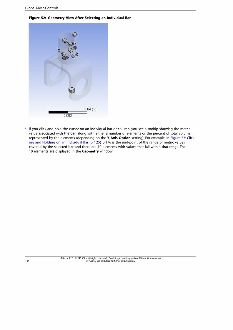
8/10/2019 ANSYS Meshing Users Guide
http://slidepdf.com/reader/full/ansys-meshing-users-guide 132/491
Figure 52: Geometry View After Selecting an Individual Bar
• If you click and hold the cursor on an individual bar or column, you see a tooltip showing the metricvalue associated with the bar, along with either a number of elements or the percent of total volume
represented by the elements (depending on the Y-Axis Option setting). For example, in Figure 53: Click-ing and Holding on an Individual Bar (p. 125), 0.176 is the mid-point of the range of metric valuescovered by the selected bar, and there are 10 elements with values that fall within that range. The10 elements are displayed in the Geometry window.
Release 15.0 - © SAS IP, Inc. All rights reserved. - Contains proprietary and confidential informationof ANSYS, Inc. and its subsidiaries and affiliates.124
Global Mesh Controls
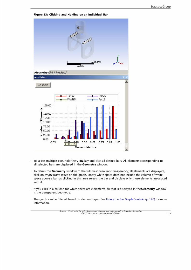
8/10/2019 ANSYS Meshing Users Guide
http://slidepdf.com/reader/full/ansys-meshing-users-guide 133/491
Figure 53: Clicking and Holding on an Individual Bar
• To select multiple bars, hold the CTRL key and click all desired bars. All elements corresponding toall selected bars are displayed in the Geometry window.
• To return the Geometry window to the full mesh view (no transparency; all elements are displayed),click on empty white space on the graph. Empty white space does not include the column of whitespace above a bar, as clicking in this area selects the bar and displays only those elements associated
with it.
• If you click in a column for which there are 0 elements, all that is displayed in the Geometry windowis the transparent geometry.
• The graph can be filtered based on element types. See Using the Bar Graph Controls (p. 126) for moreinformation.
125Release 15.0 - © SAS IP, Inc. All rights reserved. - Contains proprietary and confidential informationof ANSYS, Inc. and its subsidiaries and affiliates.
Statistics Group
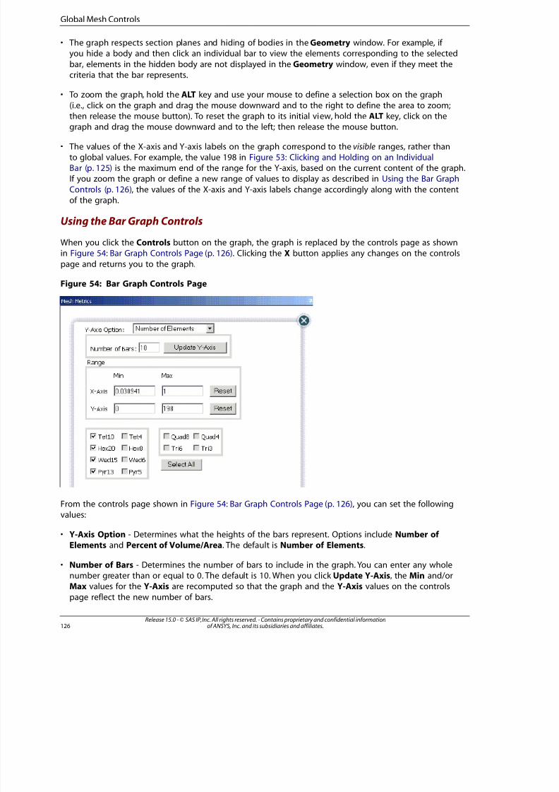
8/10/2019 ANSYS Meshing Users Guide
http://slidepdf.com/reader/full/ansys-meshing-users-guide 134/491
• The graph respects section planes and hiding of bodies in the Geometry window. For example, if you hide a body and then click an individual bar to view the elements corresponding to the selected
bar, elements in the hidden body are not displayed in the Geometry window, even if they meet thecriteria that the bar represents.
• To zoom the graph, hold the ALT key and use your mouse to define a selection box on the graph
(i.e., click on the graph and drag the mouse downward and to the right to define the area to zoom;then release the mouse button). To reset the graph to its initial view, hold the ALT key, click on the
graph and drag the mouse downward and to the left; then release the mouse button.
• The values of the X-axis and Y-axis labels on the graph correspond to the visible ranges, rather thanto global values. For example, the value 198 in Figure 53: Clicking and Holding on an IndividualBar (p. 125) is the maximum end of the range for the Y-axis, based on the current content of the graph.If you zoom the graph or define a new range of values to display as described in Using the Bar Graph
Controls (p. 126), the values of the X-axis and Y-axis labels change accordingly along with the contentof the graph.
Using the Bar Graph Controls
When you click the Controls button on the graph, the graph is replaced by the controls page as shownin Figure 54: Bar Graph Controls Page (p. 126). Clicking the X button applies any changes on the controls
page and returns you to the graph.
Figure 54: Bar Graph Controls Page
From the controls page shown in Figure 54: Bar Graph Controls Page (p. 126), you can set the following
values:
• Y-Axis Option - Determines what the heights of the bars represent. Options include Number of Elements and Percent of Volume/Area. The default is Number of Elements.
• Number of Bars - Determines the number of bars to include in the graph. You can enter any wholenumber greater than or equal to 0. The default is 10. When you click Update Y-Axis, the Min and/orMax values for the Y-Axis are recomputed so that the graph and the Y-Axis values on the controls
page reflect the new number of bars.
Release 15.0 - © SAS IP, Inc. All rights reserved. - Contains proprietary and confidential informationof ANSYS, Inc. and its subsidiaries and affiliates.126
Global Mesh Controls

8/10/2019 ANSYS Meshing Users Guide
http://slidepdf.com/reader/full/ansys-meshing-users-guide 135/491
• Range - Defines a range for the selected metric to display only those elements that fall within thespecified range.
– X-Axis - Specify a Min and/or Max value. To locate and estimate the number of worst elementsin the mesh, adjust the Min and Max values to the lower or upper end of the quality criterion(depending on metric) and click Update Y-Axis. (Determining the distribution and location of all
the bad elements at one time is helpful in cases where you may need to re-import your model intothe DesignModeler application to remove the corresponding problematic geometry.) Click Reset
to return to the X-Axis defaults. (Note: Negative values are acceptable.)
– Y-Axis - Specify a Min and/or Max value. By lowering the Max value, you can clip the Y-axis foreasier visualization of small bars, especially as they relate to different element types. Click Resetto return to the Y-Axis defaults.
• List of element types - Determines which element types to include in the graph. Element types that
do not appear in the mesh are read-only on the controls page. Select the element types that youwant to include in the graph, or click Select All to include all available element types in the graph.By default, all available element types are selected.
Calculation Details
For information about the calculations that are performed for each metric, refer to:
Element QualityAspect Ratio Calculation for TrianglesAspect Ratio Calculation for Quadrilaterals
Jacobian RatioWarping FactorParallel DeviationMaximum Corner Angle
SkewnessOrthogonal Quality
Element Quality
The Element Quality option provides a composite quality metric that ranges between 0 and 1. Thismetric is based on the ratio of the volume to the sum of the square of the edge lengths for 2D quad/tri
elements, or the square root of the cube of the sum of the square of the edge lengths for 3D elements.A value of 1 indicates a perfect cube or square while a value of 0 indicates that the element has a zeroor negative volume.
This can also be expressed as follows:
• For two-dimensional quad/tri elements:
= ∑
Note
If the Jacobian Ratio is less than zero, an error occurs.
• For three-dimensional brick elements:
127Release 15.0 - © SAS IP, Inc. All rights reserved. - Contains proprietary and confidential informationof ANSYS, Inc. and its subsidiaries and affiliates.
Statistics Group
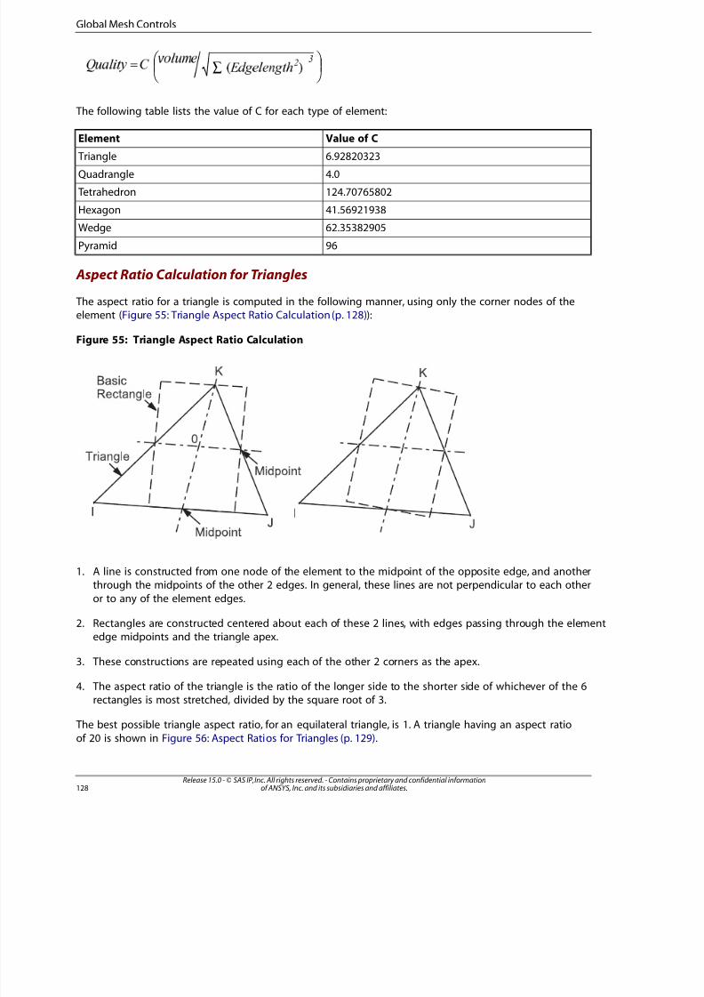
8/10/2019 ANSYS Meshing Users Guide
http://slidepdf.com/reader/full/ansys-meshing-users-guide 136/491
= ∑
The following table lists the value of C for each type of element:
Value of CElement
6.92820323 Triangle4.0Quadrangle
124.70765802 Tetrahedron
41.56921938Hexagon
62.35382905Wedge
96Pyramid
Aspect Ratio Calculation for Triangles
The aspect ratio for a triangle is computed in the following manner, using only the corner nodes of the
element (Figure 55: Triangle Aspect Ratio Calculation (p. 128)):
Figure 55: Triangle Aspect Ratio Calculation
I
J
K
B a s i c
R e c t a n g l e
T r i a n g l e
M i d p o i n t
M i d p o i n t
0
I
J
K
1. A line is constructed from one node of the element to the midpoint of the opposite edge, and anotherthrough the midpoints of the other 2 edges. In general, these lines are not perpendicular to each other
or to any of the element edges.
2. Rectangles are constructed centered about each of these 2 lines, with edges passing through the elementedge midpoints and the triangle apex.
3. These constructions are repeated using each of the other 2 corners as the apex.
4. The aspect ratio of the triangle is the ratio of the longer side to the shorter side of whichever of the 6rectangles is most stretched, divided by the square root of 3.
The best possible triangle aspect ratio, for an equilateral triangle, is 1. A triangle having an aspect ratio
of 20 is shown in Figure 56: Aspect Ratios for Triangles (p. 129).
Release 15.0 - © SAS IP, Inc. All rights reserved. - Contains proprietary and confidential informationof ANSYS, Inc. and its subsidiaries and affiliates.128
Global Mesh Controls
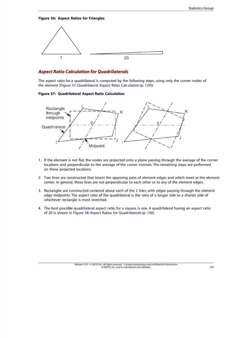
8/10/2019 ANSYS Meshing Users Guide
http://slidepdf.com/reader/full/ansys-meshing-users-guide 137/491
Figure 56: Aspect Ratios for Triangles
1
2 0
Aspect Ratio Calculation for Quadrilaterals
The aspect ratio for a quadrilateral is computed by the following steps, using only the corner nodes of the element (Figure 57: Quadrilateral Aspect Ratio Calculation (p. 129)):
Figure 57: Quadrilateral Aspect Ratio Calculation
L
K
J
I
0
L
K
J
I
0
R e c t a n g l e
t h r o u g h
m i d p o i n t s
Q u a d r i l a t e r a l
M i d p o i n t
1. If the element is not flat, the nodes are projected onto a plane passing through the average of the cornlocations and perpendicular to the average of the corner normals. The remaining steps are performed
on these projected locations.
2. Two lines are constructed that bisect the opposing pairs of element edges and which meet at the elemcenter. In general, these lines are not perpendicular to each other or to any of the element edges.
3. Rectangles are constructed centered about each of the 2 lines, with edges passing through the elemenedge midpoints. The aspect ratio of the quadrilateral is the ratio of a longer side to a shorter side of whichever rectangle is most stretched.
4. The best possible quadrilateral aspect ratio, for a square, is one. A quadrilateral having an aspect ratio
of 20 is shown in Figure 58: Aspect Ratios for Quadrilaterals (p. 130).
129Release 15.0 - © SAS IP, Inc. All rights reserved. - Contains proprietary and confidential informationof ANSYS, Inc. and its subsidiaries and affiliates.
Statistics Group

8/10/2019 ANSYS Meshing Users Guide
http://slidepdf.com/reader/full/ansys-meshing-users-guide 138/491
Figure 58: Aspect Ratios for Quadrilaterals
1 2 0
Jacobian Ratio
Jacobian ratio is computed and tested for all elements except triangles and tetrahedra that (a) are linear(have no midside nodes) or (b) have perfectly centered midside nodes. A high ratio indicates that themapping between element space and real space is becoming computationally unreliable.
Jacobian Ratio Calculation
An element's Jacobian ratio is computed by the following steps, using the full set of nodes for the ele-ment:
1. At each sampling location listed in the table below, the determinant of the Jacobian matrix is computed
and called RJ. RJ at a given point represents the magnitude of the mapping function between element
natural coordinates and real space. In an ideally-shaped element, RJ is relatively constant over the element,
and does not change sign.
R J Sampling LocationsElement Shape
Corner nodes10-node tetrahedra
base corner nodes and near apex node (apex RJ factored so that a pyramid
having all edges the same length will produce a Jacobian ratio of 1)
5-node or 13-nodepyramids
corner nodes and centroid8-node quadrilaterals
all nodes and centroid20-node bricks
corner nodesall other elements
2. The Jacobian ratio of the element is the ratio of the maximum to the minimum sampled value of RJ. If
the maximum and minimum have opposite signs, the Jacobian ratio is arbitrarily assigned to be -100
(and the element is clearly unacceptable).
3. If the element is a midside-node tetrahedron, an additional RJ is computed for a fictitious straight-sidedtetrahedron connected to the 4 corner nodes. If that RJ differs in sign from any nodal RJ (an extremely
rare occurrence), the Jacobian ratio is arbitrarily assigned to be -100.
4. If the element is a line element having a midside node, the Jacobian matrix is not square (because themapping is from one natural coordinate to 2-D or 3-D space) and has no determinant. For this case, a
vector calculation is used to compute a number which behaves like a Jacobian ratio. This calculation hasthe effect of limiting the arc spanned by a single element to about 106°.
Release 15.0 - © SAS IP, Inc. All rights reserved. - Contains proprietary and confidential informationof ANSYS, Inc. and its subsidiaries and affiliates.130
Global Mesh Controls
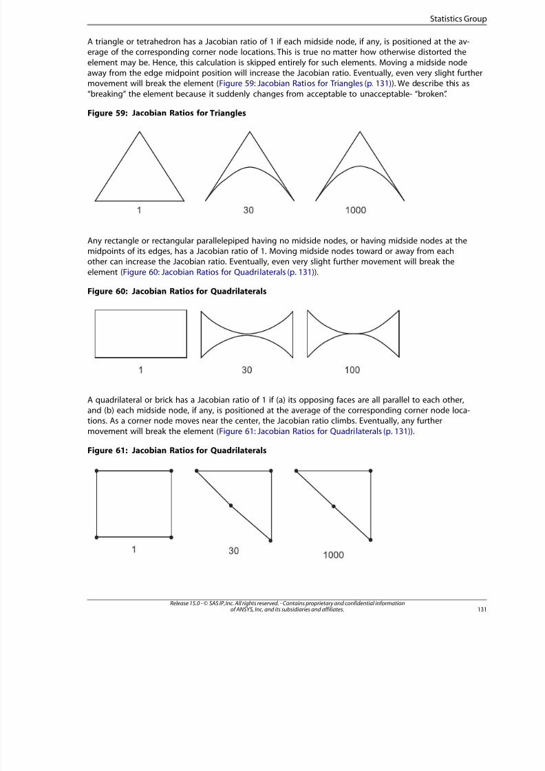
8/10/2019 ANSYS Meshing Users Guide
http://slidepdf.com/reader/full/ansys-meshing-users-guide 139/491
A triangle or tetrahedron has a Jacobian ratio of 1 if each midside node, if any, is positioned at the av-erage of the corresponding corner node locations. This is true no matter how otherwise distorted the
element may be. Hence, this calculation is skipped entirely for such elements. Moving a midside nodeaway from the edge midpoint position will increase the Jacobian ratio. Eventually, even very slight furthermovement will break the element (Figure 59: Jacobian Ratios for Triangles (p. 131)). We describe this as
“breaking” the element because it suddenly changes from acceptable to unacceptable- “broken”.
Figure 59: Jacobian Ratios for Triangles
1 3 0 1 0 0 0
Any rectangle or rectangular parallelepiped having no midside nodes, or having midside nodes at themidpoints of its edges, has a Jacobian ratio of 1. Moving midside nodes toward or away from eachother can increase the Jacobian ratio. Eventually, even very slight further movement will break the
element (Figure 60: Jacobian Ratios for Quadrilaterals (p. 131)).
Figure 60: Jacobian Ratios for Quadrilaterals
1 3 0 1 0 0
A quadrilateral or brick has a Jacobian ratio of 1 if (a) its opposing faces are all parallel to each other,and (b) each midside node, if any, is positioned at the average of the corresponding corner node loca-tions. As a corner node moves near the center, the Jacobian ratio climbs. Eventually, any further
movement will break the element (Figure 61: Jacobian Ratios for Quadrilaterals (p. 131)).
Figure 61: Jacobian Ratios for Quadrilaterals
1
3 0
1 0 0 0
13Release 15.0 - © SAS IP, Inc. All rights reserved. - Contains proprietary and confidential informationof ANSYS, Inc. and its subsidiaries and affiliates.
Statistics Group
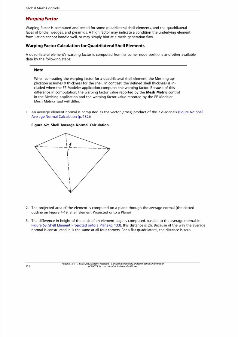
8/10/2019 ANSYS Meshing Users Guide
http://slidepdf.com/reader/full/ansys-meshing-users-guide 140/491
Warping Factor
Warping factor is computed and tested for some quadrilateral shell elements, and the quadrilateralfaces of bricks, wedges, and pyramids. A high factor may indicate a condition the underlying element
formulation cannot handle well, or may simply hint at a mesh generation flaw.
Warping Factor Calculation for Quadrilateral Shell Elements
A quadrilateral element's warping factor is computed from its corner node positions and other availabledata by the following steps:
Note
When computing the warping factor for a quadrilateral shell element, the Meshing ap-plication assumes 0 thickness for the shell. In contrast, the defined shell thickness is in-cluded when the FE Modeler application computes the warping factor. Because of thisdifference in computation, the warping factor value reported by the Mesh Metric control
in the Meshing application and the warping factor value reported by the FE ModelerMesh Metrics tool will differ.
1. An average element normal is computed as the vector (cross) product of the 2 diagonals (Figure 62: ShellAverage Normal Calculation (p. 132)).
Figure 62: Shell Average Normal Calculation
2. The projected area of the element is computed on a plane through the average normal (the dotted
outline on Figure 4-19: Shell Element Projected onto a Plane).
3. The difference in height of the ends of an element edge is computed, parallel to the average normal. InFigure 63: Shell Element Projected onto a Plane (p. 133), this distance is 2h. Because of the way the average
normal is constructed, h is the same at all four corners. For a flat quadrilateral, the distance is zero.
Release 15.0 - © SAS IP, Inc. All rights reserved. - Contains proprietary and confidential informationof ANSYS, Inc. and its subsidiaries and affiliates.132
Global Mesh Controls
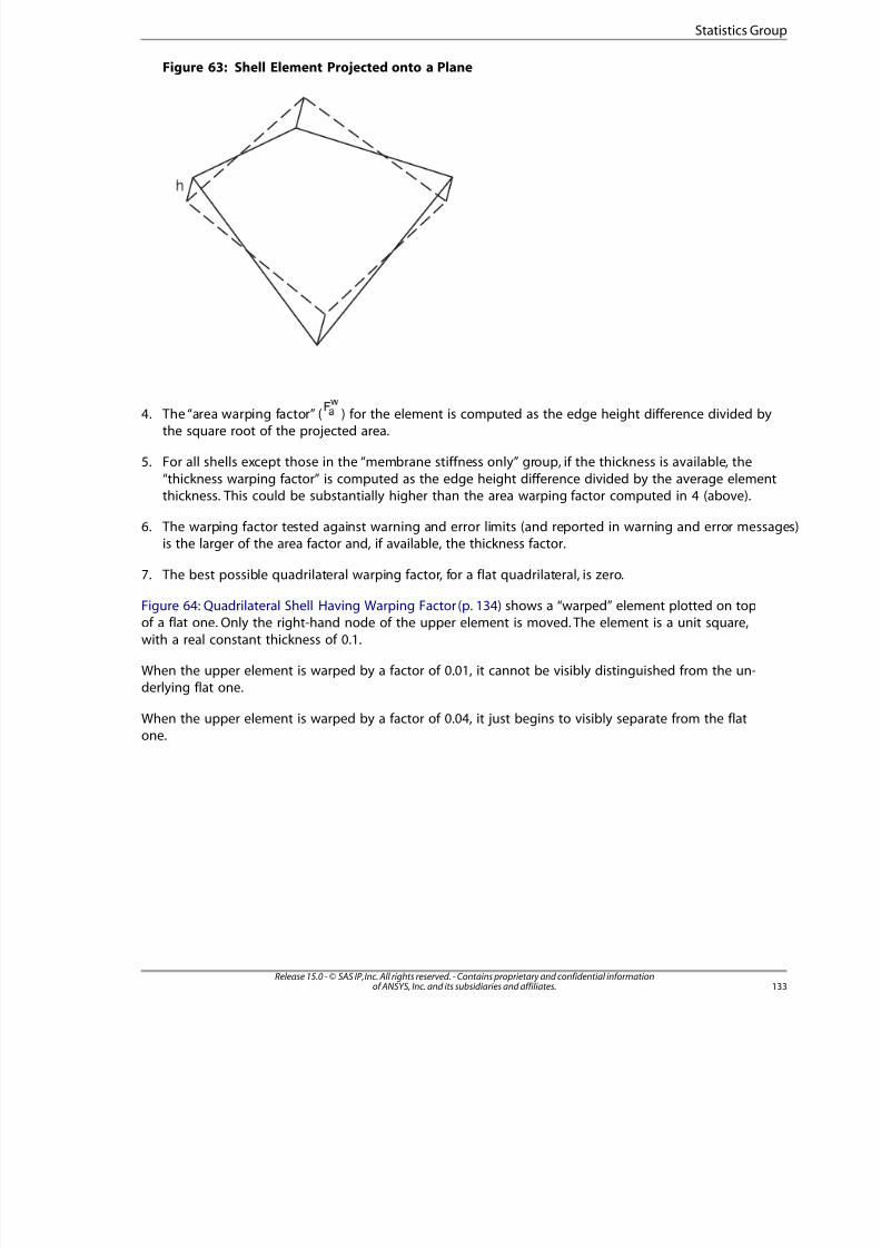
8/10/2019 ANSYS Meshing Users Guide
http://slidepdf.com/reader/full/ansys-meshing-users-guide 141/491
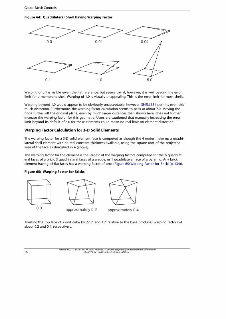
8/10/2019 ANSYS Meshing Users Guide
http://slidepdf.com/reader/full/ansys-meshing-users-guide 142/491
Figure 64: Quadrilateral Shell Having Warping Factor
0 . 0 0 . 0 1 0 . 0 4
0 . 1 1 . 0 5 . 0
Warping of 0.1 is visible given the flat reference, but seems trivial; however, it is well beyond the errorlimit for a membrane shell. Warping of 1.0 is visually unappealing. This is the error limit for most shells.
Warping beyond 1.0 would appear to be obviously unacceptable; however, SHELL181 permits even thismuch distortion. Furthermore, the warping factor calculation seems to peak at about 7.0. Moving thenode further off the original plane, even by much larger distances than shown here, does not further
increase the warping factor for this geometry. Users are cautioned that manually increasing the errorlimit beyond its default of 5.0 for these elements could mean no real limit on element distortion.
Warping Factor Calculation for 3-D Solid Elements
The warping factor for a 3-D solid element face is computed as though the 4 nodes make up a quadri-lateral shell element with no real constant thickness available, using the square root of the projected
area of the face as described in 4 (above).
The warping factor for the element is the largest of the warping factors computed for the 6 quadrilat-eral faces of a brick, 3 quadrilateral faces of a wedge, or 1 quadrilateral face of a pyramid. Any brick
element having all flat faces has a warping factor of zero ( Figure 65: Warping Factor for Bricks (p. 134)).
Figure 65: Warping Factor for Bricks
0 . 0
a p p r o x i m a t e l y 0 . 2
a p p r o x i m a t e l y 0 . 4
Twisting the top face of a unit cube by 22.5° and 45° relative to the base produces warping factors of
about 0.2 and 0.4, respectively.
Release 15.0 - © SAS IP, Inc. All rights reserved. - Contains proprietary and confidential informationof ANSYS, Inc. and its subsidiaries and affiliates.134
Global Mesh Controls
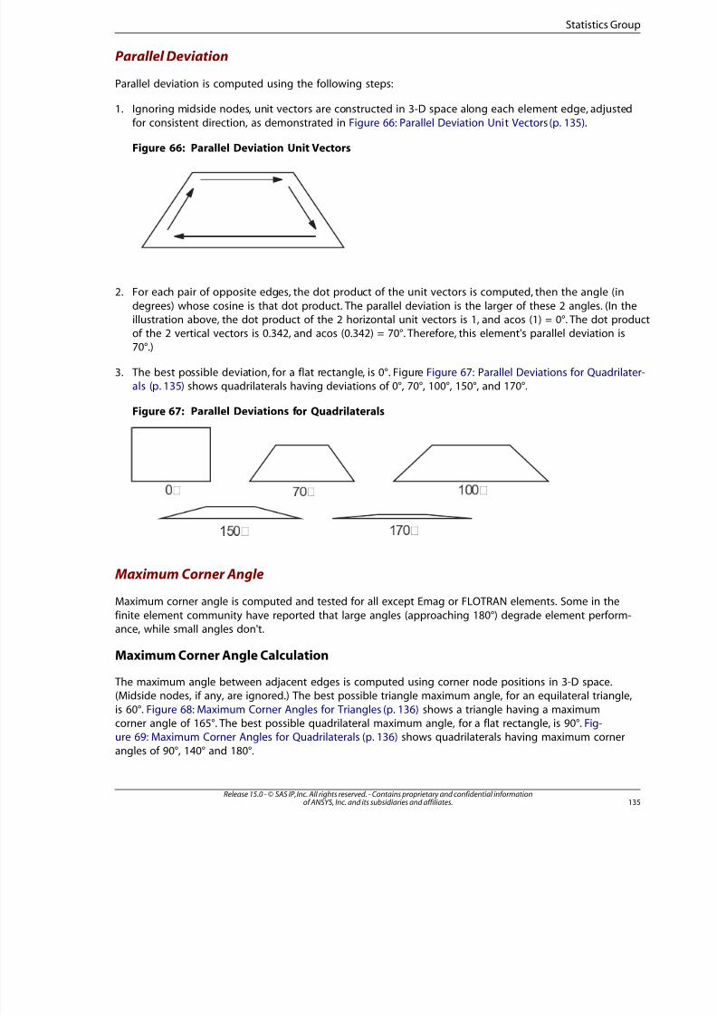
8/10/2019 ANSYS Meshing Users Guide
http://slidepdf.com/reader/full/ansys-meshing-users-guide 143/491
Parallel Deviation
Parallel deviation is computed using the following steps:
1. Ignoring midside nodes, unit vectors are constructed in 3-D space along each element edge, adjusted
for consistent direction, as demonstrated in Figure 66: Parallel Deviation Unit Vectors (p. 135).
Figure 66: Parallel Deviation Unit Vectors
2. For each pair of opposite edges, the dot product of the unit vectors is computed, then the angle (in
degrees) whose cosine is that dot product. The parallel deviation is the larger of these 2 angles. (In the
illustration above, the dot product of the 2 horizontal unit vectors is 1, and acos (1) = 0°. The dot produof the 2 vertical vectors is 0.342, and acos (0.342) = 70°. Therefore, this element's parallel deviation is70°.)
3. The best possible deviation, for a flat rectangle, is 0°. Figure Figure 67: Parallel Deviations for Quadrilateals (p. 135) shows quadrilaterals having deviations of 0°, 70°, 100°, 150°, and 170°.
Figure 67: Parallel Deviations for Quadrilaterals
Maximum Corner Angle
Maximum corner angle is computed and tested for all except Emag or FLOTRAN elements. Some in the
finite element community have reported that large angles (approaching 180°) degrade element perform-ance, while small angles don't.
Maximum Corner Angle Calculation
The maximum angle between adjacent edges is computed using corner node positions in 3-D space.(Midside nodes, if any, are ignored.) The best possible triangle maximum angle, for an equilateral triangle,
is 60°. Figure 68: Maximum Corner Angles for Triangles (p. 136) shows a triangle having a maximumcorner angle of 165°. The best possible quadrilateral maximum angle, for a flat rectangle, is 90°. Fig-ure 69: Maximum Corner Angles for Quadrilaterals (p. 136) shows quadrilaterals having maximum corner
angles of 90°, 140° and 180°.
135Release 15.0 - © SAS IP, Inc. All rights reserved. - Contains proprietary and confidential informationof ANSYS, Inc. and its subsidiaries and affiliates.
Statistics Group
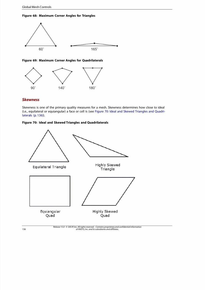
8/10/2019 ANSYS Meshing Users Guide
http://slidepdf.com/reader/full/ansys-meshing-users-guide 144/491
Figure 68: Maximum Corner Angles for Triangles
6 0 ˚ 1 6 5 ˚
Figure 69: Maximum Corner Angles for Quadrilaterals
9 0 ˚ 1 4 0 ˚ 1 8 0 ˚
Skewness
Skewness is one of the primary quality measures for a mesh. Skewness determines how close to ideal
(i.e., equilateral or equiangular) a face or cell is (see Figure 70: Ideal and Skewed Triangles and Quadri-laterals (p. 136)).
Figure 70: Ideal and Skewed Triangles and Quadrilaterals
Release 15.0 - © SAS IP, Inc. All rights reserved. - Contains proprietary and confidential informationof ANSYS, Inc. and its subsidiaries and affiliates.136
Global Mesh Controls

8/10/2019 ANSYS Meshing Users Guide
http://slidepdf.com/reader/full/ansys-meshing-users-guide 145/491
The following table lists the range of skewness values and the corresponding cell quality.
Cell QualityValue of Skewness
degenerate1
bad (sliver)0.9 — <1
poor0.75 — 0.9
fair0.5 — 0.75good0.25 — 0.5
excellent>0 — 0.25
equilateral0
According to the definition of skewness, a value of 0 indicates an equilateral cell (best) and a value of 1 indicates a completely degenerate cell (worst). Degenerate cells (slivers) are characterized by nodesthat are nearly coplanar (colinear in 2D).
Highly skewed faces and cells are unacceptable because the equations being solved assume that thecells are relatively equilateral/equiangular.
Two methods for measuring skewness are:
• Based on the equilateral volume (applies only to triangles and tetrahedra).
• Based on the deviation from a normalized equilateral angle. This method applies to all cell and faceshapes, e.g., pyramids and prisms.
Equilateral-Volume-Based Skewness
In the equilateral volume deviation method, skewness is defined as
where, the optimal cell size is the size of an equilateral cell with the same circumradius.
Quality grids have a skewness value of approximately 0.1 for 2D and 0.4 for 3D. The table above providesa general guide to the relationship between cell skewness and quality.
In 2D, all cells should be good or better. The presence of cells that are fair or worse indicates poorboundary node placement. You should try to improve your boundary mesh as much as possible, because
the quality of the overall mesh can be no better than that of the boundary mesh.
In 3D, most cells should be good or better, but a small percentage will generally be in the fair range
and there are usually even a few poor cells.
Note
The Equilateral-Volume-Based Skewness quality metric applies to any mesh element that in-cludes a triangular face. For triangular and tetrahedral elements, all faces of which are strictlytriangular, the Equilateral-Volume-Based Skewness metric applies directly. For wedge orpyramidal elements, which include combinations of triangular and quadrilateral faces, the
Meshing application computes both Equilateral-Volume-Based Skewness metrics (for the tri-
137Release 15.0 - © SAS IP, Inc. All rights reserved. - Contains proprietary and confidential informationof ANSYS, Inc. and its subsidiaries and affiliates.
Statistics Group

8/10/2019 ANSYS Meshing Users Guide
http://slidepdf.com/reader/full/ansys-meshing-users-guide 146/491
angular faces) and Normalized Equiangular Skewness metrics (for the quadrilateral faces and3-D element, itself) and reports the maximum computed metric as the element skewness.
As a result, Equilateral-Volume-Based Skewness metrics reported for meshes that containwedge and/or pyramidal elements may include skewness values attributable to NormalizedEquiangular Skewness computations.
Normalized Equiangular Skewness
In the normalized angle deviation method, skewness is defined (in general) as
θ θθ
θ θθ
−−
−
where
θmax = largest angle in the face or cell
θmin = smallest angle in the face or cell
θe = angle for an equiangular face/cell (e.g., 60 for a triangle, 90 for a square)
For a pyramid, the cell skewness will be the maximum skewness computed for any face. An ideal pyr-amid (skewness = 0) is one in which the 4 triangular faces are equilateral (and equiangular) and thequadrilateral base face is a square. The guidelines in the table above apply to the normalized equiangular
skewness as well.
Orthogonal Quality
The range for orthogonal quality is 0-1, where a value of 0 is worst and a value of 1 is best.
The orthogonal quality for cells is computed using the face normal vector, the vector from the cellcentroid to the centroid of each of the adjacent cells, and the vector from the cell centroid to each of the faces. Figure 71: Vectors Used to Compute Orthogonal Quality for a Cell (p. 139) illustrates the vectorsused to determine the orthogonal quality for a cell.
Release 15.0 - © SAS IP, Inc. All rights reserved. - Contains proprietary and confidential informationof ANSYS, Inc. and its subsidiaries and affiliates.138
Global Mesh Controls
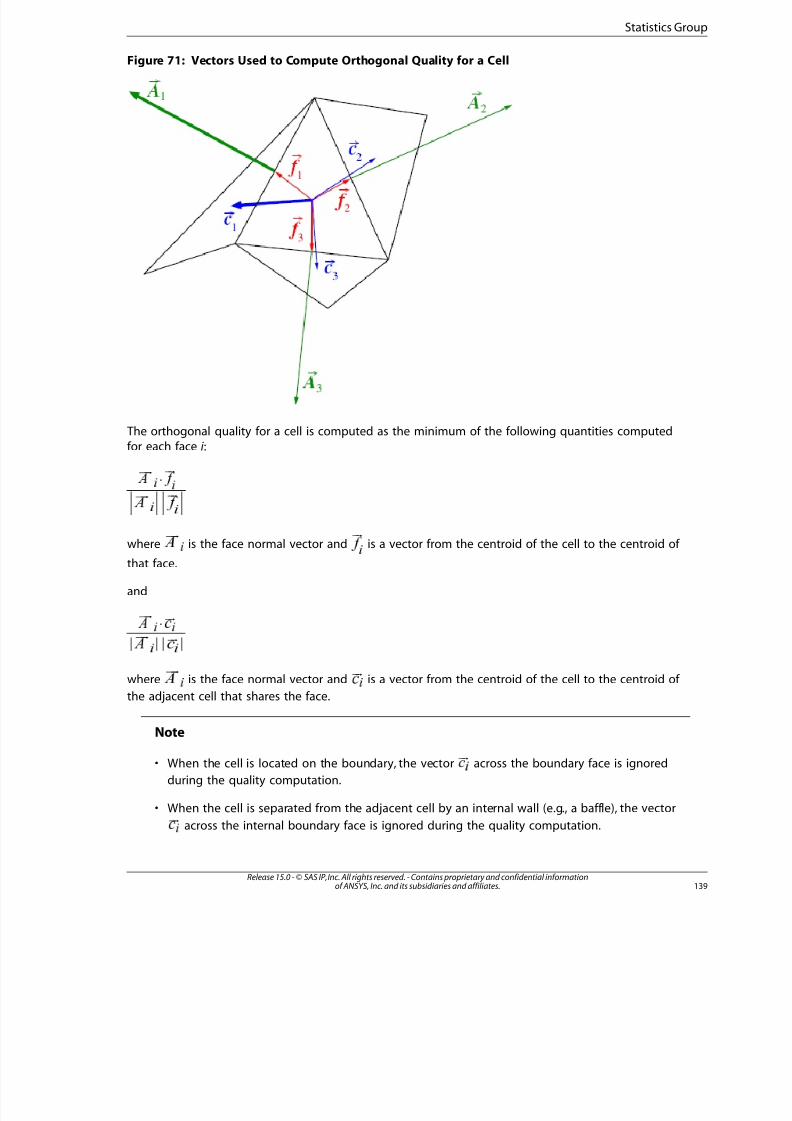
8/10/2019 ANSYS Meshing Users Guide
http://slidepdf.com/reader/full/ansys-meshing-users-guide 147/491
Figure 71: Vectors Used to Compute Orthogonal Quality for a Cell
The orthogonal quality for a cell is computed as the minimum of the following quantities computedfor each face i :
⋅
where
is the face normal vector and
is a vector from the centroid of the cell to the centroid of
that face.
and
⋅
where
is the face normal vector and
is a vector from the centroid of the cell to the centroid of
the adjacent cell that shares the face.
Note
• When the cell is located on the boundary, the vector
across the boundary face is ignored
during the quality computation.
• When the cell is separated from the adjacent cell by an internal wall (e.g., a baffle), the vector
across the internal boundary face is ignored during the quality computation.
139Release 15.0 - © SAS IP, Inc. All rights reserved. - Contains proprietary and confidential informationof ANSYS, Inc. and its subsidiaries and affiliates.
Statistics Group
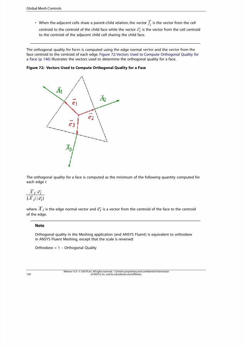
8/10/2019 ANSYS Meshing Users Guide
http://slidepdf.com/reader/full/ansys-meshing-users-guide 148/491
• When the adjacent cells share a parent-child relation, the vector
is the vector from the cell
centroid to the centroid of the child face while the vector
is the vector from the cell centroid
to the centroid of the adjacent child cell sharing the child face.
The orthogonal quality for faces is computed using the edge normal vector and the vector from the
face centroid to the centroid of each edge. Figure 72: Vectors Used to Compute Orthogonal Quality fora Face (p. 140) illustrates the vectors used to determine the orthogonal quality for a face.
Figure 72: Vectors Used to Compute Orthogonal Quality for a Face
The orthogonal quality for a face is computed as the minimum of the following quantity computed foreach edge i :
⋅
where
is the edge normal vector and
is a vector from the centroid of the face to the centroid
of the edge.
Note
Orthogonal quality in the Meshing application (and ANSYS Fluent) is equivalent to orthoskewin ANSYS Fluent Meshing, except that the scale is reversed:
Orthoskew = 1 – Orthogonal Quality
Release 15.0 - © SAS IP, Inc. All rights reserved. - Contains proprietary and confidential informationof ANSYS, Inc. and its subsidiaries and affiliates.140
Global Mesh Controls

8/10/2019 ANSYS Meshing Users Guide
http://slidepdf.com/reader/full/ansys-meshing-users-guide 149/491
The orthoskew values may not correspond exactly with the orthogonal quality values as thecomputation depends on boundary conditions on internal surfaces (WALL vs. INTERIOR /FAN /RA-
DIATOR /POROUS-JUMP ). ANSYS Fluent may return different results which reflect the modifiedmesh topology on which CFD simulations are performed. Also, for CutCell meshes, the ele-ments in the Meshing application are “traditional” (hex/tet/wedge/pyramid) elements. Whena CutCell mesh is exported from the Meshing application to ANSYS Fluent, elements that
are connected to parent faces are exported in polyhedral format, while all others retain their
type. Note that this behavior is only true for the CutCell assembly algorithm; the Tetrahedronsassembly algorithm uses only traditional element types.
14Release 15.0 - © SAS IP, Inc. All rights reserved. - Contains proprietary and confidential informationof ANSYS, Inc. and its subsidiaries and affiliates.
Statistics Group

8/10/2019 ANSYS Meshing Users Guide
http://slidepdf.com/reader/full/ansys-meshing-users-guide 150/491
8/10/2019 ANSYS Meshing Users Guide
http://slidepdf.com/reader/full/ansys-meshing-users-guide 151/491
Meshing: Local Mesh Controls
Local mesh controls are available when you highlight a Mesh object in the tree and choose a tool fromeither the Mesh Control drop-down menu, or from first choosing Insert in the context menu (displayedfrom a right mouse click on a Mesh object). You can specify the scoping of the tool in the tool's Details
View under Method to either a Geometry Selection or to a Named Selection.
Note
Be aware of the following items regarding mesh control tools:
• The Object Generator enables you to make one or more copies of a template object, scoping
each to a different piece of geometry. When defining mesh controls, you can use the Object
Generator to make copies of a template mesh control, which may reduce the necessity tomanually define multiple related mesh controls. For details, refer to Generating Multiple Objectsfrom a Template Object in the Mechanical help.
• For most mesh controls, the latest control that you add on a particular geometry overrides anyprior controls that you already have added on that geometry. For example, if you apply a Sizingcontrol setting of 0.5 to faces A,B,C then apply a setting of 1.0 to face B, faces A and C will retain
the 0.5 setting, but the setting for face B will be 1.0. This is also useful when you want to forcesweep many bodies of a multibody part and only tet mesh one or specify special sweepingoptions on one. For example, you can select all 1000 parts and then override one or 10 part(s)instead of picking 999 (990) and then selecting one (10).
Exceptions include the MultiZone Quad/Tri, MultiZone, and All Tetrahedrons - Patch Inde-pendent controls. For information about how these controls interact with other controls,refer to "Meshing: Mesh Control Interaction Tables" (p. 345), Interactions Between Mesh
Methods (p. 345), and Interactions Between Mesh Methods and Mesh Controls (p. 348).
• If you suppress a mesh control tool, the Suppress symbol appears ("x" adjacent to the nameof the tool) and Suppressed is set to Yes in the Details View of the tool. Situations can occurwhen you do not suppress a mesh control tool, and the Suppress symbol appears adjacent to
the tool but Suppressed is set to No in the Details View of the tool. In these situations, referto the mesh control's Active read-only field for the reason why the tool is suppressed. Examplesare a control applied to a uniform surface body mesh (not supported), a control scoped to
suppressed geometry, or a Contact Sizing control scoped to a suppressed Contact Region.
The following local mesh controls are available:Method ControlMesh Grouping Control
Sizing ControlContact Sizing ControlRefinement Control
Mapped Face Meshing ControlMatch Control
143Release 15.0 - © SAS IP, Inc. All rights reserved. - Contains proprietary and confidential informationof ANSYS, Inc. and its subsidiaries and affiliates.
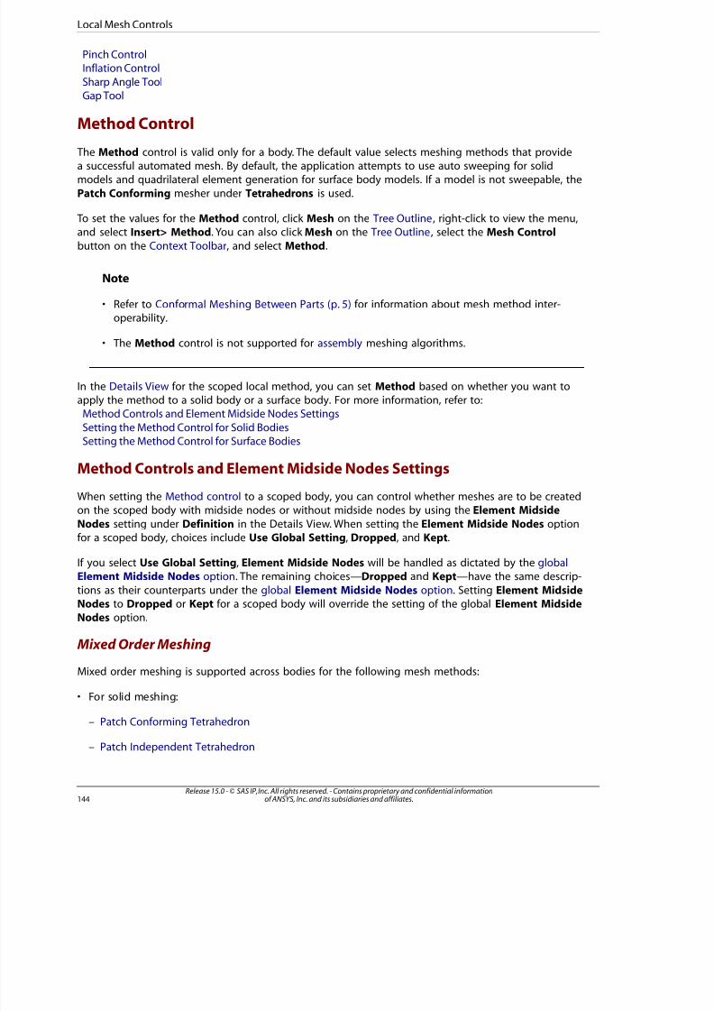
8/10/2019 ANSYS Meshing Users Guide
http://slidepdf.com/reader/full/ansys-meshing-users-guide 152/491
Pinch ControlInflation Control
Sharp Angle ToolGap Tool
Method Control
The Method control is valid only for a body. The default value selects meshing methods that providea successful automated mesh. By default, the application attempts to use auto sweeping for solidmodels and quadrilateral element generation for surface body models. If a model is not sweepable, the
Patch Conforming mesher under Tetrahedrons is used.
To set the values for the Method control, click Mesh on the Tree Outline, right-click to view the menu,and select Insert> Method. You can also click Mesh on the Tree Outline, select the Mesh Control
button on the Context Toolbar, and select Method.
Note
• Refer to Conformal Meshing Between Parts (p. 5) for information about mesh method inter-
operability.
• The Method control is not supported for assembly meshing algorithms.
In the Details View for the scoped local method, you can set Method based on whether you want toapply the method to a solid body or a surface body. For more information, refer to:
Method Controls and Element Midside Nodes Settings
Setting the Method Control for Solid BodiesSetting the Method Control for Surface Bodies
Method Controls and Element Midside Nodes SettingsWhen setting the Method control to a scoped body, you can control whether meshes are to be createdon the scoped body with midside nodes or without midside nodes by using the Element Midside
Nodes setting under Definition in the Details View. When setting the Element Midside Nodes optionfor a scoped body, choices include Use Global Setting, Dropped, and Kept.
If you select Use Global Setting, Element Midside Nodes will be handled as dictated by the globalElement Midside Nodes option. The remaining choices—Dropped and Kept—have the same descrip-
tions as their counterparts under the global Element Midside Nodes option. Setting Element MidsideNodes to Dropped or Kept for a scoped body will override the setting of the global Element MidsideNodes option.
Mixed Order Meshing
Mixed order meshing is supported across bodies for the following mesh methods:
• For solid meshing:
– Patch Conforming Tetrahedron
– Patch Independent Tetrahedron
Release 15.0 - © SAS IP, Inc. All rights reserved. - Contains proprietary and confidential informationof ANSYS, Inc. and its subsidiaries and affiliates.144
Local Mesh Controls

8/10/2019 ANSYS Meshing Users Guide
http://slidepdf.com/reader/full/ansys-meshing-users-guide 153/491
– MultiZone
– General Sweep
– Thin Sweep
– Hex Dominant
• For surface meshing:
– Quad Dominant
– All Triangles
– MultiZone Quad/Tri
This means that when scoping one of these mesh methods to bodies in a multibody part, you can setthe Element Midside Nodes option to Kept (resulting in higher order elements) for some bodies andto Dropped (resulting in lower order elements) for others. In such cases, all of the elements in a lower
order body that are adjacent to a higher order body will be higher order elements, thereby creatingone layer of quadratic elements at the interface face. These elements will be higher order at the interfaceface but with dropped midside nodes where adjacent to the linear elements in the mesh.
Note
• Mixed order meshing is not supported if you are performing Selective Meshing (p. 307). To usemixed order meshing, all of the bodies in the part must be meshed at the same time.
• To use mixed order meshing with the Patch Independent Tetrahedron, MultiZone, or MultiZoneQuad/Tri mesh methods, all of the bodies in the part must be meshed with the same mesh
method (that is, either all Patch Independent Tetrahedron, all MultiZone, or all MultiZoneQuad/Tri).
The figures below illustrate an example of mixed order meshing. To obtain the mesh shown in Fig-
ure 73: Mixed Order Meshing of a Multibody Part (p. 146), the global Element Midside Nodes optionwas set to Kept, resulting in a mesh of quadratic tet elements for the topmost body. The sweep methodwas applied to the remaining bodies, with the Element Midside Nodes option set to Dropped on theSweep Method control. This resulted in a mesh of primarily linear hex/wedge elements for the swept
bodies, with the hex/wedge elements that are attached to the common interface being mixed order(see Figure 74: Mixed Order Elements (p. 146)).
145Release 15.0 - © SAS IP, Inc. All rights reserved. - Contains proprietary and confidential informationof ANSYS, Inc. and its subsidiaries and affiliates.
Method Contro
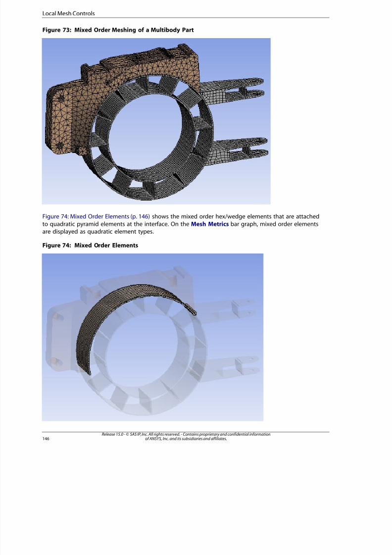
8/10/2019 ANSYS Meshing Users Guide
http://slidepdf.com/reader/full/ansys-meshing-users-guide 154/491
Figure 73: Mixed Order Meshing of a Multibody Part
Figure 74: Mixed Order Elements (p. 146) shows the mixed order hex/wedge elements that are attached
to quadratic pyramid elements at the interface. On the Mesh Metrics bar graph, mixed order elementsare displayed as quadratic element types.
Figure 74: Mixed Order Elements
Release 15.0 - © SAS IP, Inc. All rights reserved. - Contains proprietary and confidential informationof ANSYS, Inc. and its subsidiaries and affiliates.146
Local Mesh Controls
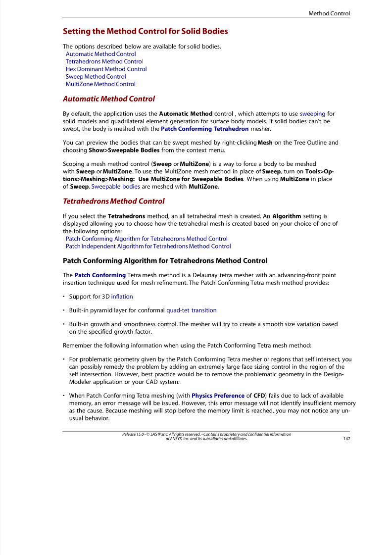
8/10/2019 ANSYS Meshing Users Guide
http://slidepdf.com/reader/full/ansys-meshing-users-guide 155/491
Setting the Method Control for Solid Bodies
The options described below are available for solid bodies.Automatic Method Control Tetrahedrons Method Control
Hex Dominant Method ControlSweep Method Control
MultiZone Method Control
Automatic Method Control
By default, the application uses the Automatic Method control , which attempts to use sweeping for
solid models and quadrilateral element generation for surface body models. If solid bodies can't beswept, the body is meshed with the Patch Conforming Tetrahedron mesher.
You can preview the bodies that can be swept meshed by right-clicking Mesh on the Tree Outline and
choosing Show>Sweepable Bodies from the context menu.
Scoping a mesh method control (Sweep or MultiZone) is a way to force a body to be meshed
with Sweep or MultiZone. To use the MultiZone mesh method in place of Sweep, turn on Tools>Op-tions>Meshing>Meshing: Use MultiZone for Sweepable Bodies. When using MultiZone in placeof Sweep, Sweepable bodies are meshed with MultiZone.
Tetrahedrons Method Control
If you select the Tetrahedrons method, an all tetrahedral mesh is created. An Algorithm setting isdisplayed allowing you to choose how the tetrahedral mesh is created based on your choice of one of
the following options:Patch Conforming Algorithm for Tetrahedrons Method ControlPatch Independent Algorithm for Tetrahedrons Method Control
Patch Conforming Algorithm for Tetrahedrons Method Control
The Patch Conforming Tetra mesh method is a Delaunay tetra mesher with an advancing-front point
insertion technique used for mesh refinement. The Patch Conforming Tetra mesh method provides:
• Support for 3D inflation
• Built-in pyramid layer for conformal quad-tet transition
• Built-in growth and smoothness control. The mesher will try to create a smooth size variation basedon the specified growth factor.
Remember the following information when using the Patch Conforming Tetra mesh method:
• For problematic geometry given by the Patch Conforming Tetra mesher or regions that self intersect, yocan possibly remedy the problem by adding an extremely large face sizing control in the region of theself intersection. However, best practice would be to remove the problematic geometry in the Design-
Modeler application or your CAD system.
• When Patch Conforming Tetra meshing (with Physics Preference of CFD) fails due to lack of availablememory, an error message will be issued. However, this error message will not identify insufficient memoas the cause. Because meshing will stop before the memory limit is reached, you may not notice any un-
usual behavior.
147Release 15.0 - © SAS IP, Inc. All rights reserved. - Contains proprietary and confidential informationof ANSYS, Inc. and its subsidiaries and affiliates.
Method Contro
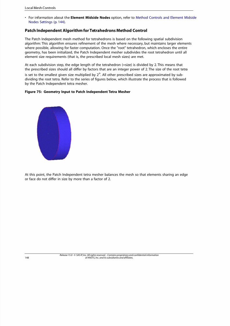
8/10/2019 ANSYS Meshing Users Guide
http://slidepdf.com/reader/full/ansys-meshing-users-guide 156/491
• For information about the Element Midside Nodes option, refer to Method Controls and Element MidsideNodes Settings (p. 144).
Patch Independent Algorithm for Tetrahedrons Method Control
The Patch Independent mesh method for tetrahedrons is based on the following spatial subdivisionalgorithm: This algorithm ensures refinement of the mesh where necessary, but maintains larger elementswhere possible, allowing for faster computation. Once the "root" tetrahedron, which encloses the entire
geometry, has been initialized, the Patch Independent mesher subdivides the root tetrahedron until allelement size requirements (that is, the prescribed local mesh sizes) are met.
At each subdivision step, the edge length of the tetrahedron (=size) is divided by 2. This means that
the prescribed sizes should all differ by factors that are an integer power of 2. The size of the root tetra
is set to the smallest given size multiplied by 2n. All other prescribed sizes are approximated by sub-
dividing the root tetra. Refer to the series of figures below, which illustrate the process that is followedby the Patch Independent tetra mesher.
Figure 75: Geometry Input to Patch Independent Tetra Mesher
At this point, the Patch Independent tetra mesher balances the mesh so that elements sharing an edgeor face do not differ in size by more than a factor of 2.
Release 15.0 - © SAS IP, Inc. All rights reserved. - Contains proprietary and confidential informationof ANSYS, Inc. and its subsidiaries and affiliates.148
Local Mesh Controls
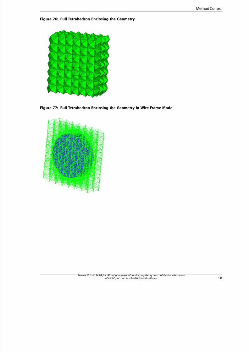
8/10/2019 ANSYS Meshing Users Guide
http://slidepdf.com/reader/full/ansys-meshing-users-guide 157/491
Figure 76: Full Tetrahedron Enclosing the Geometry
Figure 77: Full Tetrahedron Enclosing the Geometry in Wire Frame Mode
149Release 15.0 - © SAS IP, Inc. All rights reserved. - Contains proprietary and confidential informationof ANSYS, Inc. and its subsidiaries and affiliates.
Method Contro
8/10/2019 ANSYS Meshing Users Guide
http://slidepdf.com/reader/full/ansys-meshing-users-guide 158/491
Figure 78: Cross-Section of the Tetrahedron
After this is done, the Patch Independent tetra mesher makes the mesh conformal; that is, it guaranteesthat each pair of adjacent elements will share an entire face. The mesh does not yet match the given
geometry, so the mesher next rounds the nodes of the mesh to the prescribed points, prescribed curves,or model surfaces. The Patch Independent tetra mesher then "cuts away" all of the mesh, which cannotbe reached by a user-defined material point without intersection of a surface.
Figure 79: Mesh After Capture of Surfaces and Separation of Useful Volume
Release 15.0 - © SAS IP, Inc. All rights reserved. - Contains proprietary and confidential informationof ANSYS, Inc. and its subsidiaries and affiliates.150
Local Mesh Controls
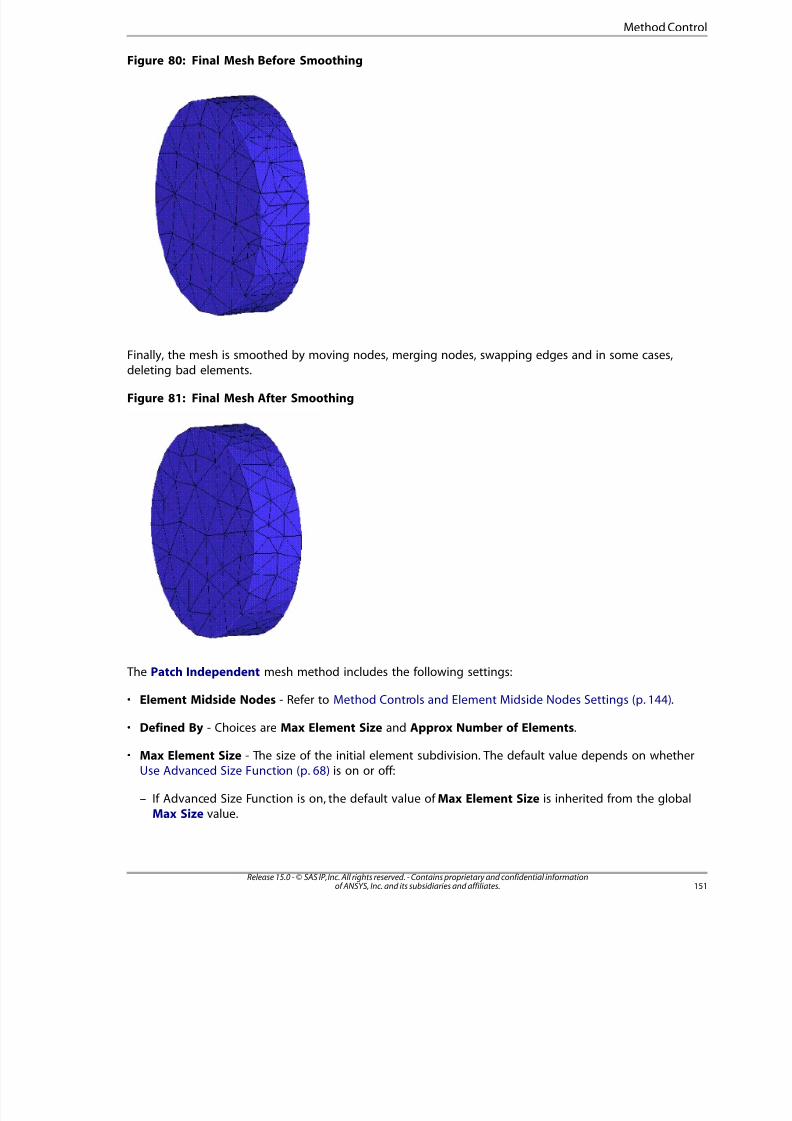
8/10/2019 ANSYS Meshing Users Guide
http://slidepdf.com/reader/full/ansys-meshing-users-guide 159/491
Figure 80: Final Mesh Before Smoothing
Finally, the mesh is smoothed by moving nodes, merging nodes, swapping edges and in some cases,deleting bad elements.
Figure 81: Final Mesh After Smoothing
The Patch Independent mesh method includes the following settings:
• Element Midside Nodes - Refer to Method Controls and Element Midside Nodes Settings (p. 144).
• Defined By - Choices are Max Element Size and Approx Number of Elements.
• Max Element Size - The size of the initial element subdivision. The default value depends on whetherUse Advanced Size Function (p. 68) is on or off:
– If Advanced Size Function is on, the default value of Max Element Size is inherited from the globalMax Size value.
15Release 15.0 - © SAS IP, Inc. All rights reserved. - Contains proprietary and confidential informationof ANSYS, Inc. and its subsidiaries and affiliates.
Method Contro

8/10/2019 ANSYS Meshing Users Guide
http://slidepdf.com/reader/full/ansys-meshing-users-guide 160/491
– If Advanced Size Function is off, the default value of Max Element Size is inherited from the globalElement Size value.
In either case, you can change the value if you want to apply a specific value locally. In such cases,the maximum size comes from the larger value of the global controls (that is, Max Size or ElementSize, as described above) OR, the largest scoped body size or face size that Patch Independent is also
scoped to. A scoped edge size is not respected if it is larger than either the global size or the size onan attached face.
With the Patch Independent mesh method, scoped body sizing is supported as follows:
– If a local body size is defined and it is smaller than the global maximum size, the scoped body sizewill be assigned inside the volume.
– If the global maximum size is smaller than any scoped body, face or edge sizing, the global max-imum size (Element Size when Advanced Size Function is off; Max Size when Advanced Size
Function is on) will be changed to be the same as the largest sizing within the mesher. For example,if Patch Independent is defined on two bodies, and the setup is as follows:
Global Max Size = 4
Local body size scoped to Body1 = 8
No local body size is scoped to Body2 The Patch Independent maximum size will be 8, and the global Max Size of 4 will be used for thesizing of Body2.
Note
The maximum element size inside the volume of Body2 could grow to 8. Sincesetting local sizings affects the largest element size in the model, it is recommended
to avoid setting local sizes that are larger than the global maximum size.
• Approx Number of Elements - Prescribes an approximate number of elements for the mesh. The default
is 5.0E+05. Specifying a prescribed number of elements for the Patch Independent method is applicableonly if the method is being applied to a single part.
• Feature Angle - Specifies the minimum angle at which geometry features will be captured. If the angle
between two faces is less than the specified Feature Angle, the edge between the faces will be ignored,and the nodes will be placed without respect to that edge. If the angle between two faces is greater thanthe Feature Angle, the edge should be retained and mesh aligned and associated with it (note the edgecould be ignored due to defeaturing, etc.). You can specify a value from 0 (capture most edges) to 90
(ignore most edges) degrees or accept the default of 30 degrees.
• Mesh Based Defeaturing - Ignores edges based on size. Off by default. If set to On, a Defeaturing Tol-erance field appears where you may enter a numerical value greater than 0.0. By default, the value of this
local Defeaturing Tolerance field is the same as the global Defeaturing Tolerance (p. 120). If you specifya different value here, it will override the global value. Specifying a value of 0.0 here resets the toleranceto its default. If multiple Patch Independent tetra mesh method controls are defined with different toler-ances, the smallest tolerance is respected.
There are several basic cases, including the following:
Release 15.0 - © SAS IP, Inc. All rights reserved. - Contains proprietary and confidential informationof ANSYS, Inc. and its subsidiaries and affiliates.152
Local Mesh Controls
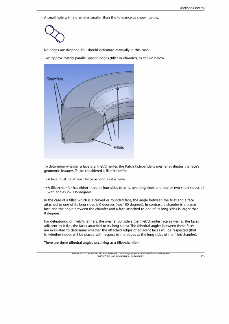
8/10/2019 ANSYS Meshing Users Guide
http://slidepdf.com/reader/full/ansys-meshing-users-guide 161/491
– A small hole with a diameter smaller than the tolerance as shown below.
No edges are dropped. You should defeature manually in this case.
– Two approximately parallel spaced edges (fillet or chamfer), as shown below.
To determine whether a face is a fillet/chamfer, the Patch Independent mesher evaluates the face'sgeometric features. To be considered a fillet/chamfer:
A face must be at least twice as long as it is wide.
A fillet/chamfer has either three or four sides (that is, two long sides and one or two short sides), allwith angles <= 135 degrees.
In the case of a fillet, which is a curved or rounded face, the angle between the fillet and a face
attached to one of its long sides is 0 degrees (not 180 degrees). In contrast, a chamfer is a planarface and the angle between the chamfer and a face attached to one of its long sides is larger than0 degrees.
For defeaturing of fillets/chamfers, the mesher considers the fillet/chamfer face as well as the faces
adjacent to it (i.e., the faces attached to its long sides). The dihedral angles between these facesare evaluated to determine whether the attached edges of adjacent faces will be respected (thatis, whether nodes will be placed with respect to the edges at the long sides of the fillet/chamfer).
There are three dihedral angles occurring at a fillet/chamfer:
153Release 15.0 - © SAS IP, Inc. All rights reserved. - Contains proprietary and confidential informationof ANSYS, Inc. and its subsidiaries and affiliates.
Method Contro
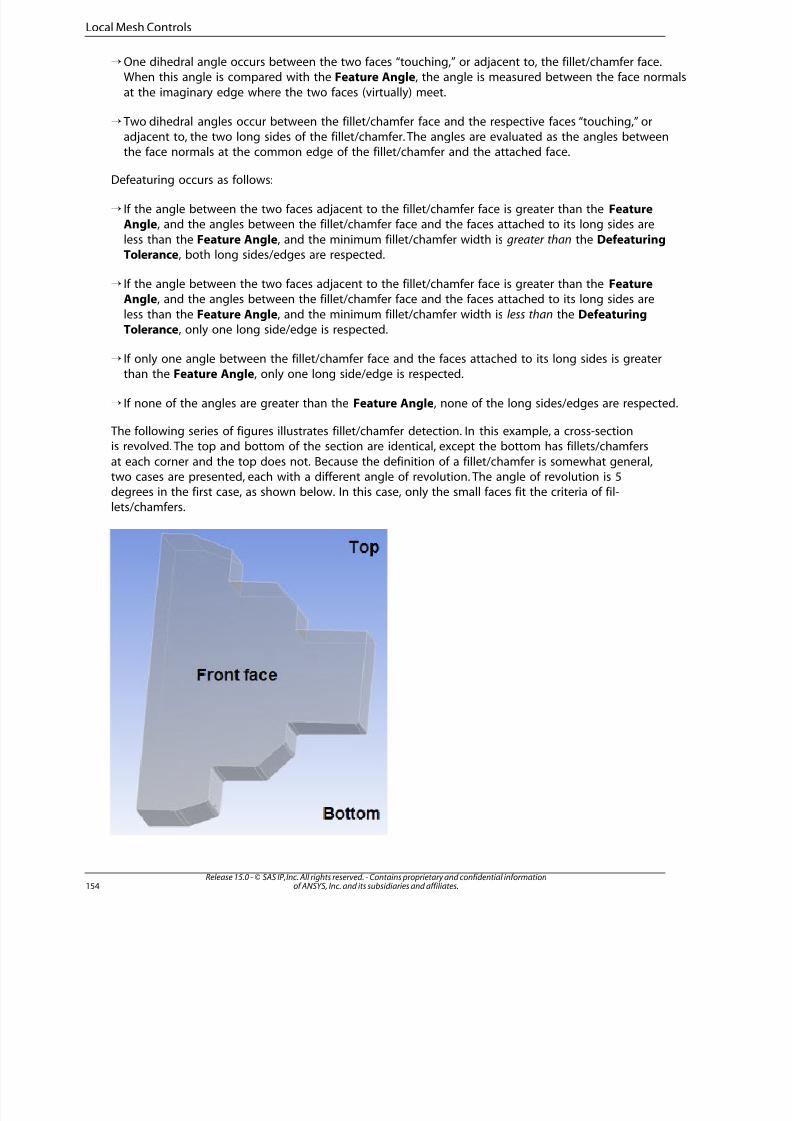
8/10/2019 ANSYS Meshing Users Guide
http://slidepdf.com/reader/full/ansys-meshing-users-guide 162/491
One dihedral angle occurs between the two faces “touching,” or adjacent to, the fillet/chamfer face.When this angle is compared with the Feature Angle, the angle is measured between the face normals
at the imaginary edge where the two faces (virtually) meet.
Two dihedral angles occur between the fillet/chamfer face and the respective faces “touching,” oradjacent to, the two long sides of the fillet/chamfer. The angles are evaluated as the angles betweenthe face normals at the common edge of the fillet/chamfer and the attached face.
Defeaturing occurs as follows:
If the angle between the two faces adjacent to the fillet/chamfer face is greater than the FeatureAngle, and the angles between the fillet/chamfer face and the faces attached to its long sides are
less than the Feature Angle, and the minimum fillet/chamfer width is greater than the DefeaturingTolerance, both long sides/edges are respected.
If the angle between the two faces adjacent to the fillet/chamfer face is greater than the FeatureAngle, and the angles between the fillet/chamfer face and the faces attached to its long sides are
less than the Feature Angle, and the minimum fillet/chamfer width is less than the DefeaturingTolerance, only one long side/edge is respected.
If only one angle between the fillet/chamfer face and the faces attached to its long sides is greaterthan the Feature Angle, only one long side/edge is respected.
If none of the angles are greater than the Feature Angle, none of the long sides/edges are respected.
The following series of figures illustrates fillet/chamfer detection. In this example, a cross-sectionis revolved. The top and bottom of the section are identical, except the bottom has fillets/chamfers
at each corner and the top does not. Because the definition of a fillet/chamfer is somewhat general,two cases are presented, each with a different angle of revolution. The angle of revolution is 5degrees in the first case, as shown below. In this case, only the small faces fit the criteria of fil-lets/chamfers.
Release 15.0 - © SAS IP, Inc. All rights reserved. - Contains proprietary and confidential informationof ANSYS, Inc. and its subsidiaries and affiliates.154
Local Mesh Controls
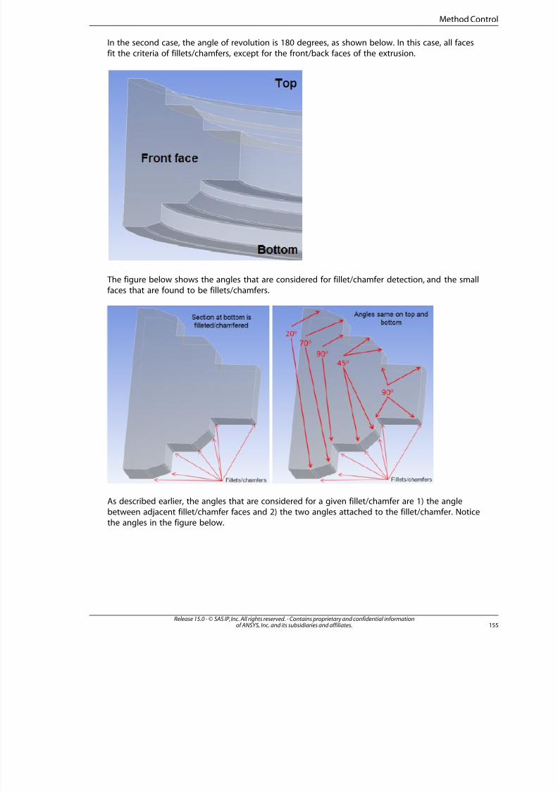
8/10/2019 ANSYS Meshing Users Guide
http://slidepdf.com/reader/full/ansys-meshing-users-guide 163/491
In the second case, the angle of revolution is 180 degrees, as shown below. In this case, all facesfit the criteria of fillets/chamfers, except for the front/back faces of the extrusion.
The figure below shows the angles that are considered for fillet/chamfer detection, and the smallfaces that are found to be fillets/chamfers.
As described earlier, the angles that are considered for a given fillet/chamfer are 1) the anglebetween adjacent fillet/chamfer faces and 2) the two angles attached to the fillet/chamfer. Noticethe angles in the figure below.
155Release 15.0 - © SAS IP, Inc. All rights reserved. - Contains proprietary and confidential informationof ANSYS, Inc. and its subsidiaries and affiliates.
Method Contro
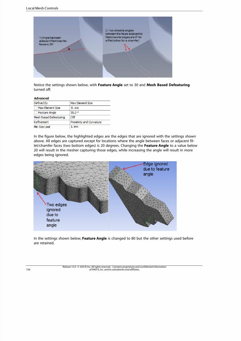
8/10/2019 ANSYS Meshing Users Guide
http://slidepdf.com/reader/full/ansys-meshing-users-guide 164/491
Notice the settings shown below, with Feature Angle set to 30 and Mesh Based Defeaturingturned off.
In the figure below, the highlighted edges are the edges that are ignored with the settings shownabove. All edges are captured except for locations where the angle between faces or adjacent fil-let/chamfer faces (two bottom edges) is 20 degrees. Changing the Feature Angle to a value below20 will result in the mesher capturing those edges, while increasing the angle will result in more
edges being ignored.
In the settings shown below, Feature Angle is changed to 80 but the other settings used beforeare retained.
Release 15.0 - © SAS IP, Inc. All rights reserved. - Contains proprietary and confidential informationof ANSYS, Inc. and its subsidiaries and affiliates.156
Local Mesh Controls
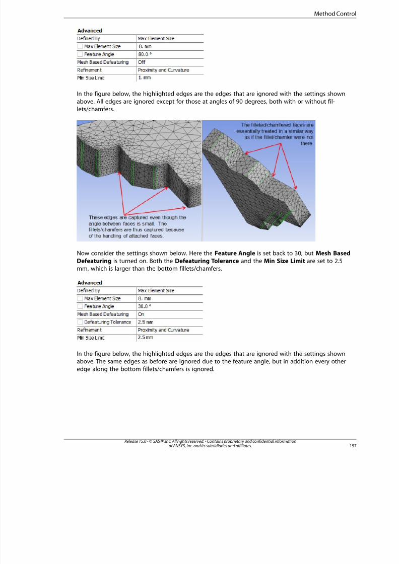
8/10/2019 ANSYS Meshing Users Guide
http://slidepdf.com/reader/full/ansys-meshing-users-guide 165/491
In the figure below, the highlighted edges are the edges that are ignored with the settings shown
above. All edges are ignored except for those at angles of 90 degrees, both with or without fil-lets/chamfers.
Now consider the settings shown below. Here the Feature Angle is set back to 30, but Mesh Based
Defeaturing is turned on. Both the Defeaturing Tolerance and the Min Size Limit are set to 2.5mm, which is larger than the bottom fillets/chamfers.
In the figure below, the highlighted edges are the edges that are ignored with the settings shownabove. The same edges as before are ignored due to the feature angle, but in addition every otheredge along the bottom fillets/chamfers is ignored.
157Release 15.0 - © SAS IP, Inc. All rights reserved. - Contains proprietary and confidential informationof ANSYS, Inc. and its subsidiaries and affiliates.
Method Contro
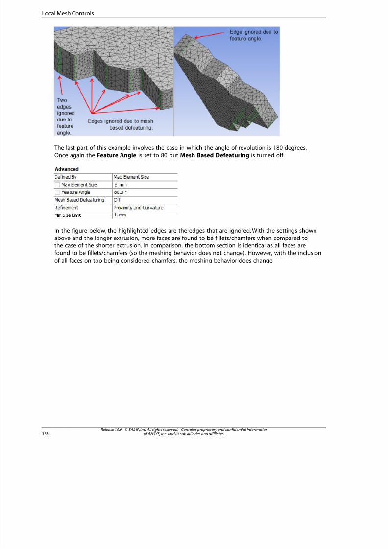
8/10/2019 ANSYS Meshing Users Guide
http://slidepdf.com/reader/full/ansys-meshing-users-guide 166/491
The last part of this example involves the case in which the angle of revolution is 180 degrees.Once again the Feature Angle is set to 80 but Mesh Based Defeaturing is turned off.
In the figure below, the highlighted edges are the edges that are ignored. With the settings shown
above and the longer extrusion, more faces are found to be fillets/chamfers when compared tothe case of the shorter extrusion. In comparison, the bottom section is identical as all faces arefound to be fillets/chamfers (so the meshing behavior does not change). However, with the inclusion
of all faces on top being considered chamfers, the meshing behavior does change.
Release 15.0 - © SAS IP, Inc. All rights reserved. - Contains proprietary and confidential informationof ANSYS, Inc. and its subsidiaries and affiliates.158
Local Mesh Controls
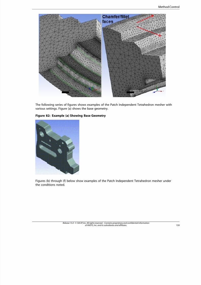
8/10/2019 ANSYS Meshing Users Guide
http://slidepdf.com/reader/full/ansys-meshing-users-guide 167/491
The following series of figures shows examples of the Patch Independent Tetrahedron mesher withvarious settings. Figure (a) shows the base geometry.
Figure 82: Example (a) Showing Base Geometry
Figures (b) through (f) below show examples of the Patch Independent Tetrahedron mesher under
the conditions noted.
159Release 15.0 - © SAS IP, Inc. All rights reserved. - Contains proprietary and confidential informationof ANSYS, Inc. and its subsidiaries and affiliates.
Method Contro
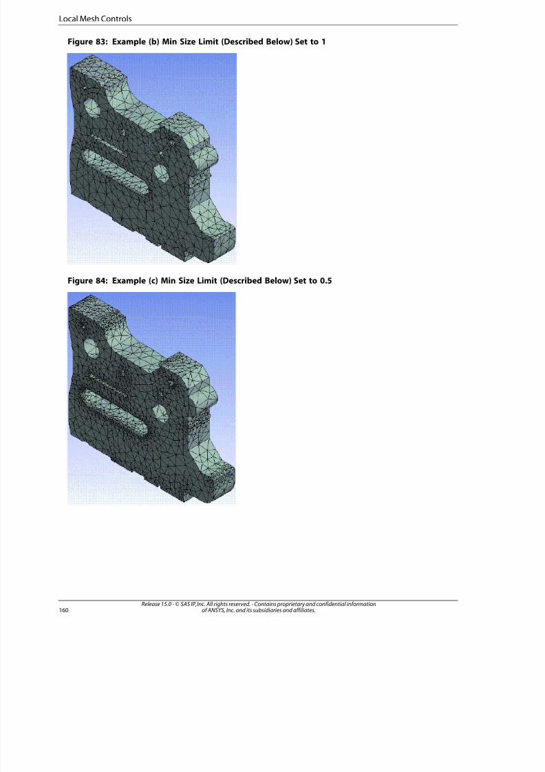
8/10/2019 ANSYS Meshing Users Guide
http://slidepdf.com/reader/full/ansys-meshing-users-guide 168/491
Figure 83: Example (b) Min Size Limit (Described Below) Set to 1
Figure 84: Example (c) Min Size Limit (Described Below) Set to 0.5
Release 15.0 - © SAS IP, Inc. All rights reserved. - Contains proprietary and confidential informationof ANSYS, Inc. and its subsidiaries and affiliates.160
Local Mesh Controls
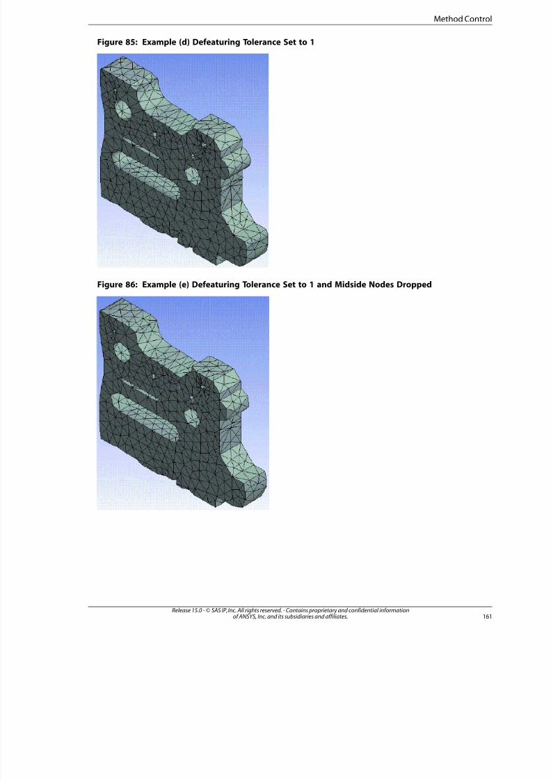
8/10/2019 ANSYS Meshing Users Guide
http://slidepdf.com/reader/full/ansys-meshing-users-guide 169/491
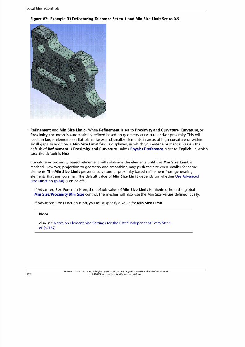
8/10/2019 ANSYS Meshing Users Guide
http://slidepdf.com/reader/full/ansys-meshing-users-guide 170/491
Figure 87: Example (f) Defeaturing Tolerance Set to 1 and Min Size Limit Set to 0.5
• Refinement and Min Size Limit - When Refinement is set to Proximity and Curvature, Curvature, or
Proximity, the mesh is automatically refined based on geometry curvature and/or proximity. This willresult in larger elements on flat planar faces and smaller elements in areas of high curvature or withinsmall gaps. In addition, a Min Size Limit field is displayed, in which you enter a numerical value. (Thedefault of Refinement is Proximity and Curvature, unless Physics Preference is set to Explicit, in which
case the default is No.)
Curvature or proximity based refinement will subdivide the elements until this Min Size Limit isreached. However, projection to geometry and smoothing may push the size even smaller for some
elements. The Min Size Limit prevents curvature or proximity based refinement from generatingelements that are too small. The default value of Min Size Limit depends on whether Use AdvancedSize Function (p. 68) is on or off:
– If Advanced Size Function is on, the default value of Min Size Limit is inherited from the global
Min Size /Proximity Min Size control. The mesher will also use the Min Size values defined locally.
– If Advanced Size Function is off, you must specify a value for Min Size Limit.
Note
Also see Notes on Element Size Settings for the Patch Independent Tetra Mesh-
er (p. 167).
Release 15.0 - © SAS IP, Inc. All rights reserved. - Contains proprietary and confidential informationof ANSYS, Inc. and its subsidiaries and affiliates.162
Local Mesh Controls
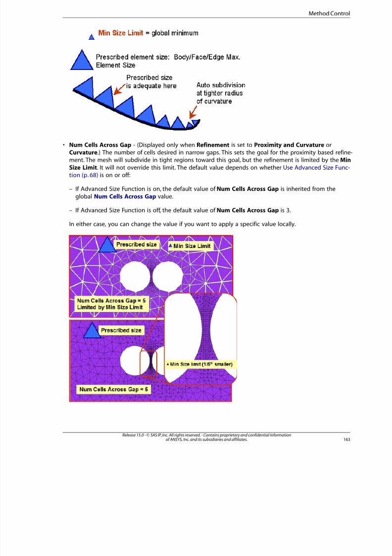
8/10/2019 ANSYS Meshing Users Guide
http://slidepdf.com/reader/full/ansys-meshing-users-guide 171/491
• Num Cells Across Gap - (Displayed only when Refinement is set to Proximity and Curvature orCurvature.) The number of cells desired in narrow gaps. This sets the goal for the proximity based refinement. The mesh will subdivide in tight regions toward this goal, but the refinement is limited by the Min
Size Limit. It will not override this limit. The default value depends on whether Use Advanced Size Func-
tion (p. 68) is on or off:
– If Advanced Size Function is on, the default value of Num Cells Across Gap is inherited from the
global Num Cells Across Gap value.
– If Advanced Size Function is off, the default value of Num Cells Across Gap is 3.
In either case, you can change the value if you want to apply a specific value locally.
163Release 15.0 - © SAS IP, Inc. All rights reserved. - Contains proprietary and confidential informationof ANSYS, Inc. and its subsidiaries and affiliates.
Method Contro
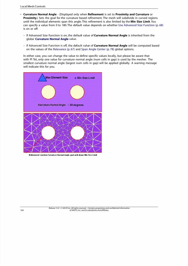
8/10/2019 ANSYS Meshing Users Guide
http://slidepdf.com/reader/full/ansys-meshing-users-guide 172/491
• Curvature Normal Angle - (Displayed only when Refinement is set to Proximity and Curvature orProximity.) Sets the goal for the curvature based refinement. The mesh will subdivide in curved regions
until the individual elements span this angle. This refinement is also limited by the Min Size Limit. Youcan specify a value from 0 to 180. The default value depends on whether Use Advanced Size Function (p. 68)is on or off:
– If Advanced Size Function is on, the default value of Curvature Normal Angle is inherited from theglobal Curvature Normal Angle value.
– If Advanced Size Function is off, the default value of Curvature Normal Angle will be computed based
on the values of the Relevance (p. 67) and Span Angle Center (p. 78) global options.
In either case, you can change the value to define specific values locally, but please be aware thatwith PI Tet, only one value for curvature normal angle (num cells in gap) is used by the mesher. Thesmallest curvature normal angle (largest num cells in gap) will be applied globally. A warning message
will indicate this for you.
Release 15.0 - © SAS IP, Inc. All rights reserved. - Contains proprietary and confidential informationof ANSYS, Inc. and its subsidiaries and affiliates.164
Local Mesh Controls
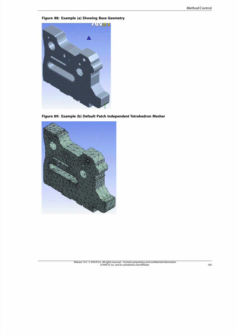
8/10/2019 ANSYS Meshing Users Guide
http://slidepdf.com/reader/full/ansys-meshing-users-guide 173/491
Figure 88: Example (a) Showing Base Geometry
Figure 89: Example (b) Default Patch Independent Tetrahedron Mesher
165Release 15.0 - © SAS IP, Inc. All rights reserved. - Contains proprietary and confidential informationof ANSYS, Inc. and its subsidiaries and affiliates.
Method Contro
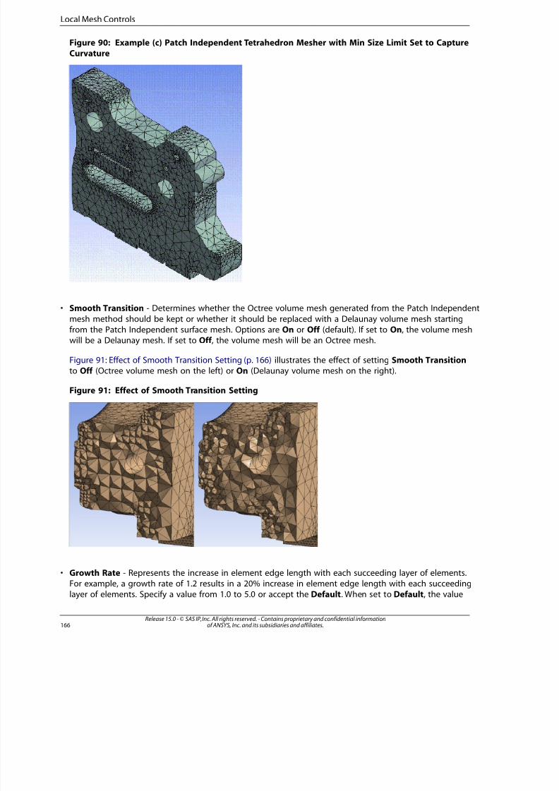
8/10/2019 ANSYS Meshing Users Guide
http://slidepdf.com/reader/full/ansys-meshing-users-guide 174/491
Figure 90: Example (c) Patch Independent Tetrahedron Mesher with Min Size Limit Set to CaptureCurvature
• Smooth Transition - Determines whether the Octree volume mesh generated from the Patch Independent
mesh method should be kept or whether it should be replaced with a Delaunay volume mesh startingfrom the Patch Independent surface mesh. Options are On or Off (default). If set to On, the volume meshwill be a Delaunay mesh. If set to Off , the volume mesh will be an Octree mesh.
Figure 91: Effect of Smooth Transition Setting (p. 166) illustrates the effect of setting Smooth Transition
to Off (Octree volume mesh on the left) or On (Delaunay volume mesh on the right).
Figure 91: Effect of Smooth Transition Setting
• Growth Rate - Represents the increase in element edge length with each succeeding layer of elements.For example, a growth rate of 1.2 results in a 20% increase in element edge length with each succeedinglayer of elements. Specify a value from 1.0 to 5.0 or accept the Default. When set to Default, the value
Release 15.0 - © SAS IP, Inc. All rights reserved. - Contains proprietary and confidential informationof ANSYS, Inc. and its subsidiaries and affiliates.166
Local Mesh Controls
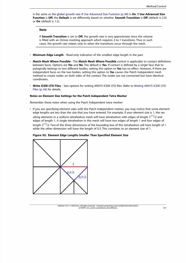
8/10/2019 ANSYS Meshing Users Guide
http://slidepdf.com/reader/full/ansys-meshing-users-guide 175/491
is the same as the global growth rate if Use Advanced Size Function (p. 68) is On. If Use Advanced SizeFunction is Off , the Default is set differently based on whether Smooth Transition is Off (default is 2.0
or On (default is 1.2).
Note
If Smooth Transition is set to Off , the growth rate is very approximate since the volume
is filled with an Octree meshing approach which requires 2-to-1 transitions. Thus in suchcases, the growth rate relates only to when the transitions occur through the mesh.
• Minimum Edge Length - Read-only indication of the smallest edge length in the part.
• Match Mesh Where Possible - The Match Mesh Where Possible control is applicable to contact definitbetween faces. Options are Yes and No. The default is Yes. If contact is defined by a single face that to-
pologically belongs to two different bodies, setting this option to Yes has no effect. However, if there areindependent faces on the two bodies, setting this option to Yes causes the Patch Independent meshmethod to create nodes on both sides of the contact. The nodes are not connected but have identical
coordinates.
• Write ICEM CFD Files - Sets options for writing ANSYS ICEM CFD files. Refer to Writing ANSYS ICEM CFDFiles (p. 56) for details.
Notes on Element Size Settings for the Patch Independent Tetra Mesher
Remember these notes when using the Patch Independent tetra mesher:
• If you are specifying element sizes with the Patch Independent mesher, you may notice that some elemeedge lengths are less than the size that you have entered. For example, if your element size is 1, the res-
ulting elements in a uniform tetrahedron mesh will have tetrahedron with edges of length 31/2
/2 andedges of length 1. A single tetrahedron in this mesh will have two edges of length 1 and four edges of
length 31/2 /2. Two of the three dimensions of the bounding box of this tetrahedron will have length of 1while the other dimension will have the length of 0.5. This correlates to an element size of 1.
Figure 92: Element Edge Lengths Smaller Than Specified Element Size
167Release 15.0 - © SAS IP, Inc. All rights reserved. - Contains proprietary and confidential informationof ANSYS, Inc. and its subsidiaries and affiliates.
Method Contro

8/10/2019 ANSYS Meshing Users Guide
http://slidepdf.com/reader/full/ansys-meshing-users-guide 176/491
• If you are using Curvature and Proximity Refinement, you may notice that your elements are always lessthan the maximum size specified. Element growth rates with this mesher are always based on powers of
2. For instance if your minimum size limit is set to 1 and your maximum element size limit is set to 5, andyou have curvature in your model that warrants curvature based mesh refinement down to the minimumelement size, you will see that the largest elements are not size 5 but size 4. This happens because in order
to maintain elements at the minimum size limit, the initial tetrahedron must be some power of 2 largerthan the minimum element size, which in this example case is 1.
• Small features of Named Selections will be checked in comparison to element size settings prior tomeshing. If the minimum element size seems to be too big to capture the essential features of the geometry,
a warning will be issued if small entities could cause the mesher to fail.
Notes on Scoping for the Patch Independent Mesher
You can use the Patch Independent tetra mesh method in combination with other solid mesh methods
in a multibody part, and the bodies will be meshed with conformal mesh. Refer to Conformal MeshingBetween Parts (p. 5) for information about conformal meshing and mesh method interoperability.
Notes on Virtual Topologies and the Patch Independent Mesher
Virtual topologies may affect the success of meshing with the Patch Independent tetra mesh method.Because virtual topologies are often a coarse approximation of the original faces or edges, the resultingsmall inaccuracies (gaps and overlaps) may cause the Patch Independent tetra mesher to miss someparts of the boundary of the virtual topology. As a result, the mesher may not accurately model the
respected topology and may fail.
Since in general, the Patch Independent tetra mesh method does not require the use of virtual topologiesto clean up the geometry, you can remove some of the problematic virtual topology and use Named
Selections for boundary conditions instead, as appropriate.
Miscellaneous Notes for the Patch Independent Mesher
The Patch Independent tetra mesh method does not support mesh connections, pinch controls, matchcontrols, or mapped face meshing controls.
Hex Dominant Method Control
If you select the Hex Dominant method, a free hex dominant mesh is created. If you are interested ina hex mesh, this option is recommended for bodies that cannot be swept. To preview any bodies thatcan be swept, click Mesh on the Tree Outline and right-click the mouse. Select Show> Sweepable
Bodies from the context menu to display bodies that fulfill the requirements of a sweepable body(other than axis sweeping).
The Hex Dominant mesh method includes the following settings:
• Element Midside Nodes - Refer to Method Controls and Element Midside Nodes Settings (p. 144).
• Free Face Mesh Type - Determines the shape of the elements used to fill the body. Allows you tochoose Quad/Tri or All Quad. The default is Quad/Tri.
Hex dominant meshing adds the most value under the following conditions:
• Meshing bodies with large amounts of interior volume.
Release 15.0 - © SAS IP, Inc. All rights reserved. - Contains proprietary and confidential informationof ANSYS, Inc. and its subsidiaries and affiliates.168
Local Mesh Controls
8/10/2019 ANSYS Meshing Users Guide
http://slidepdf.com/reader/full/ansys-meshing-users-guide 177/491
• Meshing bodies that transition from sweepable bodies in a body that has been decomposed for sweepiHowever, it is better to use Body /Face Sizing to obtain more uniform face meshing, which leads to more
hexes by volume.
Hex dominant meshing adds little value under the following conditions:
• Meshing thin complicated bodies (like a cellular phone case). The number of elements may actually incr
compared to a tetrahedron mesh since the element size must be much smaller for this class of body whe
using hex dominant meshing to create well shaped hexes.
• A body is sweepable or can easily be decomposed to multiple sweepable bodies. The quality of a swept
mesh is usually superior to that of a hex dominant mesh.
• Models where fast transition of the mesh can result in poor solution accuracy (e.g. CFD models). The Hexdominant approach can have very fast transitions at the core of the volume.
Note
• Mesh Matching for cyclic symmetry is not supported for hex dominant meshing.
• Workbench assists you in determining if hex dominant meshing is applicable to your situation.When you apply the Hex Dominant option on a body or group of bodies, Workbench calculatesthe normalized volume to surface area ratio (p. 169). If it detects a ratio less than 2, Control
Message appears in a highlighted row under Definition in the Details View. If you click Yes,Click To Display, a warning message states that a low percentage of hex elements or poorlyshaped hex elements may result. Suggestions are included for alternative meshing schemes.
The normalized volume to surface area ratio is defined by the following expression:
(Volume of body/(Surface area of body)3/2
)/factor
where factor, the ratio for a unit sphere = (4/3π
)/(4π
)
3/2
• Adaptive refinement starting from a hex dominant mesh will result in remeshing of the structure
with tetrahedrons.
• If you apply a local Sizing control to a solid body with a Method control set to Hex Dominantor Sweep, or to a sheet body with a Method control set to Quadrilateral Dominant, a nearuniform quadrilateral mesh will result on all affected faces on a body meshed with Hex Dom-
inant, on the source face meshed with Sweep, and on all affected faces meshed with Quadri-lateral Dominant. To obtain even more of a uniform quadrilateral mesh, set the Behavior of the Sizing control to Hard.
Sweep Method Control
If you select the Sweep method, a swept mesh is forced on “sweepable” bodies (including axis-sweepable
bodies, which are not displayed when you use the Show Sweepable Bodies feature). The mesher willfail if a swept mesh cannot be generated on a body with a Sweep Method control.
Use the Sweep option for any of the following situations:
• A swept mesh is required.
169Release 15.0 - © SAS IP, Inc. All rights reserved. - Contains proprietary and confidential informationof ANSYS, Inc. and its subsidiaries and affiliates.
Method Contro
8/10/2019 ANSYS Meshing Users Guide
http://slidepdf.com/reader/full/ansys-meshing-users-guide 178/491

8/10/2019 ANSYS Meshing Users Guide
http://slidepdf.com/reader/full/ansys-meshing-users-guide 179/491
In some cases, the thin model sweeper may want to swap source and target faces basedon meshing conditions in neighboring bodies. In such cases, a warning message will be
issued to alert you.
For example, if you are mixing a patch independent mesh method (i.e., Patch Inde-pendent tetra or MultiZone) with the thin model sweeper to mesh bodies in amultibody part, the thin model sweeper may need to swap the source and target
faces in order to respect protected topology in the neighboring bodies. If there isprotected topology on both sides of the body that is scoped for thin sweep, the sidewith the largest number of faces is selected as the source face.
To make source/target face selection easier, select View > Annotations from the MainMenu to toggle the visibility of annotations in the Geometry window. For example, afterscoping Sweep to a body, the body will be displayed using a blue solid annotation. SelectView > Annotations to turn off the annotations; then select the source/target faces. For
picking internal faces, the Hide Faces right mouse button option may help you to see insidea body. For example, you can select external faces in the Geometry window and then usethe Hide Faces option to hide the selected faces (making it easier to select the internalfaces).
Refer to Considerations for Selecting Source Faces for the Thin Model Sweeper (p. 239) for details.
• Free Face Mesh Type - Determines the shape of the elements used to fill the swept body (pure hex, purwedge, or a combination of hex/wedge). Allows you to choose All Tri, Quad/Tri, or All Quad meshing
when Src/Trg Selection is Automatic, Manual Source, or Manual Source and Target. Allows you tochoose Quad/Tri or All Quad meshing when Src/Trg Selection is Automatic Thin or Manual Thin. Thedefault in all cases is Quad/Tri.
Note
– If the source face is also a side face of another body, the face will always be quad mapped.
– When Free Face Mesh Type is set to either Quad/Tri or All Quad and the source face canbe mapped meshed, the face will sometimes be mapped meshed even if it means appliedsizing controls (such as Contact Sizing, Sphere of Influence, etc.) will be ignored.
– In some cases when Src/Trg Selection is set to Automatic, the source face that is selectedby the software must be quad mapped in order for the sweep method to be successful. Inthese cases, the value that is specified for Free Face Mesh Type may be ignored.
• Type - Allows you to specify a Number of Divisions or Element Size through the sweep direction. Whe
sweeping generalized bodies that share faces, the Element Size is a soft constraint on interval assignmeand the Number of Divisions is a hard constraint. If you have conflicting Number of Divisions constraithe sweeper will fail and yield a message. To obtain a regular mesh in the sweep direction, the guiding
edges must have consistent lengths. You can define virtual split edges to achieve consistent lengths forthese edges (see Creating and Managing Virtual Split Edges (p. 374)). Also see Sizing Control (p. 181) formore information.
• Sweep Bias Type - Specify bias in the same manner as edge biasing for the Bias Type setting in a Sizin
mesh control. There is no graphical feedback for biasing on a Method control. Biasing direction is basedfrom the source to the target.
17Release 15.0 - © SAS IP, Inc. All rights reserved. - Contains proprietary and confidential informationof ANSYS, Inc. and its subsidiaries and affiliates.
Method Contro
8/10/2019 ANSYS Meshing Users Guide
http://slidepdf.com/reader/full/ansys-meshing-users-guide 180/491
• The Constrain Boundary setting is available for multibody parts only (both for general sweeping andthin sweeping). Specify whether you want to allow the mesher to split the elements at the boundary of
a swept mesh region to aid in meshing. You can choose Yes (constrain boundary; no splitting is allowed)or No (do not constrain boundary; splitting is allowed). Choosing Yes prevents tets from entering theswept body. The default is No.
Note
• For gasket simulations, set the Stiffness Behavior of the body to Gasket and proceed withadjusting mesh settings as described in the Gasket Mesh Control section located under Gasketsin the Mechanical application help.
• In models with swept regions, the Advanced Size Function will affect the mesh gradation in
the swept region. You can override this effect by specifying any Sweep Bias value (includinga value of 1), Sweep Element Size value, or Sweep Num Divs value in the Details View whendefining the sweep method.
• There is a system limitation when using the sweep method with the Advanced Size Function. The Advanced Size Function may have nodes slightly off because the spacing is queried. The
sweeper then tries to match that spacing, which may lead to unexpected mesh results.
• If you apply a local Sizing control to a solid body with a Method control set to Hex Dominantor Sweep, or to a sheet body with a Method control set to Quadrilateral Dominant, a nearuniform quadrilateral mesh will result on all affected faces on a body meshed with Hex Dom-inant, on the source face meshed with Sweep, and on all affected faces meshed with Quadri-
lateral Dominant. To obtain even more of a uniform quadrilateral mesh, set the Behavior of the Sizing control to Hard.
MultiZone Method Control
The MultiZone mesh method, which is a patch independent meshing technique, provides automaticdecomposition of geometry into mapped (sweepable) regions and free regions. When the MultiZone
mesh method is selected, all regions are meshed with a pure hexahedral mesh if possible. To handlecases in which a pure hex mesh will not be possible, you can adjust your settings so that a swept meshwill be generated in structured regions and a free mesh will be generated in unstructured regions.
For example, using the Sweep mesh method, you would need to slice the part below into five bodies
as shown to obtain a pure hex mesh:
Note
This section describes method control settings. See MultiZone Meshing (p. 251) for detailedalgorithm and usage information.
Release 15.0 - © SAS IP, Inc. All rights reserved. - Contains proprietary and confidential informationof ANSYS, Inc. and its subsidiaries and affiliates.172
Local Mesh Controls
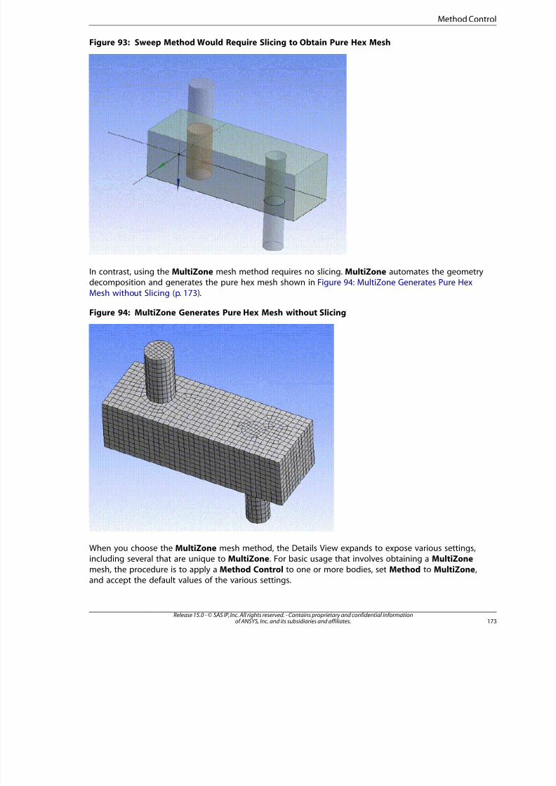
8/10/2019 ANSYS Meshing Users Guide
http://slidepdf.com/reader/full/ansys-meshing-users-guide 181/491
Figure 93: Sweep Method Would Require Slicing to Obtain Pure Hex Mesh
In contrast, using the MultiZone mesh method requires no slicing. MultiZone automates the geometrydecomposition and generates the pure hex mesh shown in Figure 94: MultiZone Generates Pure Hex
Mesh without Slicing (p. 173).
Figure 94: MultiZone Generates Pure Hex Mesh without Slicing
When you choose the MultiZone mesh method, the Details View expands to expose various settings,including several that are unique to MultiZone. For basic usage that involves obtaining a MultiZone
mesh, the procedure is to apply a Method Control to one or more bodies, set Method to MultiZone,and accept the default values of the various settings.
173Release 15.0 - © SAS IP, Inc. All rights reserved. - Contains proprietary and confidential informationof ANSYS, Inc. and its subsidiaries and affiliates.
Method Contro

8/10/2019 ANSYS Meshing Users Guide
http://slidepdf.com/reader/full/ansys-meshing-users-guide 182/491
For advanced or specialized usage, adjust the settings as needed. The following is a description of eachof these settings.
• Mapped Mesh Type - Determines the shape of the elements used to fill structured regions according tothe following choices (the default is Hexa):
– Hexa - A mesh of all hexahedral elements is generated for the part the method is scoped to.
– Hexa/Prism - A mesh of hexahedral and prism/wedge elements is generated for the part the methodis scoped to. The main difference between the Hexa/Prism option and the other options is that forswept regions, the surface mesh can allow triangles for quality and transitioning. The triangles are later
extruded to prisms/wedges.
– Prism - A mesh of all prism elements is generated for the part the method is scoped to. This option issometimes useful if the source face mesh is being shared with a tet mesh, as pyramids are not requiredto transition to the tet mesh.
• Surface Mesh Method - Specifying a value for Surface Mesh Method instructs MultiZone to use theProgram Controlled, Uniform, or Pave method to create the surface mesh.
– Program Controlled - Automatically uses a combination of Uniform and Pave mesh methods dependingon the mesh sizes set and face properties. This is the default method.
– Uniform - Uses a recursive loop-splitting method which creates a highly uniform mesh. This option isgenerally good when all edges have the same sizing and the faces being meshed do not have a high
degree of curvature. The orthogonality of the mesh from this method is generally very good.
– Pave - Uses a paving mesh method which creates a good quality mesh on faces with high curvature,and also when neighboring edges have a high aspect ratio. This approach is also more reliable to givean all-quad mesh.
Note
The Surface Mesh Method is applicable only to faces that are free meshed. If a face canbe mapped meshed, it will be. However, you can force a free mesh on a face by definingdifferent hard sizing controls on opposite edges of the face.
Note
Models created in versions of ANSYS older than ANSYS 14.5 that have a MultiZone mesh
method defined on them will be resumed in ANSYS 14.5 with the Surface Mesh Methodset to Uniform, so that the mesh is similar to what it was in previous versions. You mightwant to set the Surface Mesh Method to Program Controlled for better results.
• Free Mesh Type - Specifying a value for Free Mesh Type will instruct MultiZone to allow a free mesh if it is not possible (without slicing) to generate a pure hex or hex/prism mesh. The value of Free MeshType determines the shape of the elements used to fill unstructured regions according to the followingchoices (the default is Not Allowed):
– Not Allowed - Choose this option if you require a mapped mesh.
Release 15.0 - © SAS IP, Inc. All rights reserved. - Contains proprietary and confidential informationof ANSYS, Inc. and its subsidiaries and affiliates.174
Local Mesh Controls
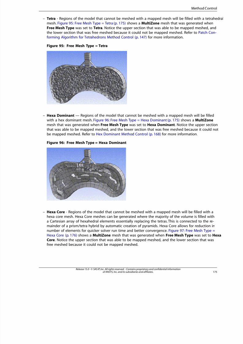
8/10/2019 ANSYS Meshing Users Guide
http://slidepdf.com/reader/full/ansys-meshing-users-guide 183/491
– Tetra - Regions of the model that cannot be meshed with a mapped mesh will be filled with a tetrahemesh. Figure 95: Free Mesh Type = Tetra (p. 175) shows a MultiZone mesh that was generated when
Free Mesh Type was set to Tetra. Notice the upper section that was able to be mapped meshed, andthe lower section that was free meshed because it could not be mapped meshed. Refer to Patch Con-forming Algorithm for Tetrahedrons Method Control (p. 147) for more information.
Figure 95: Free Mesh Type = Tetra
– Hexa Dominant — Regions of the model that cannot be meshed with a mapped mesh will be filledwith a hex dominant mesh. Figure 96: Free Mesh Type = Hexa Dominant (p. 175) shows a MultiZonemesh that was generated when Free Mesh Type was set to Hexa Dominant. Notice the upper section
that was able to be mapped meshed, and the lower section that was free meshed because it could nobe mapped meshed. Refer to Hex Dominant Method Control (p. 168) for more information.
Figure 96: Free Mesh Type = Hexa Dominant
– Hexa Core - Regions of the model that cannot be meshed with a mapped mesh will be filled with a
hexa core mesh. Hexa Core meshes can be generated where the majority of the volume is filled witha Cartesian array of hexahedral elements essentially replacing the tetras. This is connected to the re-mainder of a prism/tetra hybrid by automatic creation of pyramids. Hexa Core allows for reduction in
number of elements for quicker solver run time and better convergence. Figure 97: Free Mesh Type =Hexa Core (p. 176) shows a MultiZone mesh that was generated when Free Mesh Type was set to HeCore. Notice the upper section that was able to be mapped meshed, and the lower section that wasfree meshed because it could not be mapped meshed.
175Release 15.0 - © SAS IP, Inc. All rights reserved. - Contains proprietary and confidential informationof ANSYS, Inc. and its subsidiaries and affiliates.
Method Contro
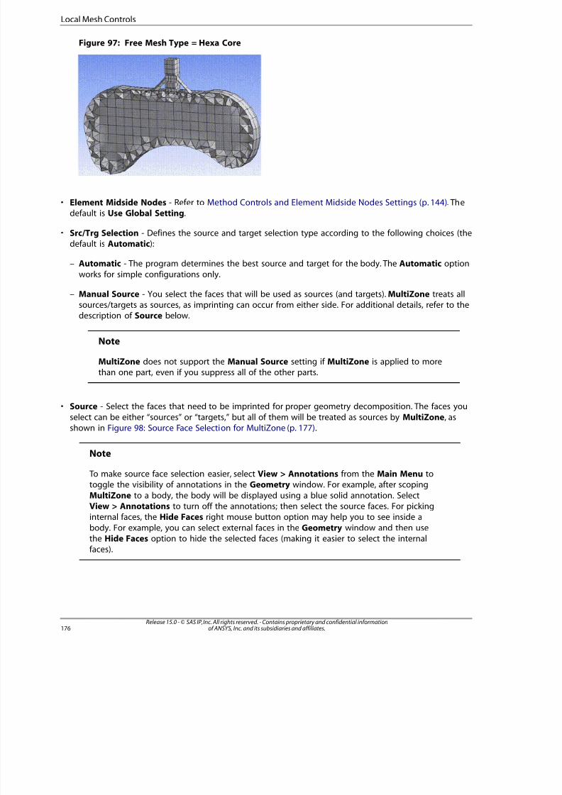
8/10/2019 ANSYS Meshing Users Guide
http://slidepdf.com/reader/full/ansys-meshing-users-guide 184/491
Figure 97: Free Mesh Type = Hexa Core
• Element Midside Nodes - Refer to Method Controls and Element Midside Nodes Settings (p. 144). Thedefault is Use Global Setting.
• Src/Trg Selection - Defines the source and target selection type according to the following choices (thedefault is Automatic):
– Automatic - The program determines the best source and target for the body. The Automatic option
works for simple configurations only.
– Manual Source - You select the faces that will be used as sources (and targets). MultiZone treats allsources/targets as sources, as imprinting can occur from either side. For additional details, refer to thedescription of Source below.
Note
MultiZone does not support the Manual Source setting if MultiZone is applied to more
than one part, even if you suppress all of the other parts.
• Source - Select the faces that need to be imprinted for proper geometry decomposition. The faces you
select can be either “sources” or “targets,” but all of them will be treated as sources by MultiZone, asshown in Figure 98: Source Face Selection for MultiZone (p. 177).
Note
To make source face selection easier, select View > Annotations from the Main Menu totoggle the visibility of annotations in the Geometry window. For example, after scoping
MultiZone to a body, the body will be displayed using a blue solid annotation. SelectView > Annotations to turn off the annotations; then select the source faces. For pickinginternal faces, the Hide Faces right mouse button option may help you to see inside a
body. For example, you can select external faces in the Geometry window and then usethe Hide Faces option to hide the selected faces (making it easier to select the internalfaces).
Release 15.0 - © SAS IP, Inc. All rights reserved. - Contains proprietary and confidential informationof ANSYS, Inc. and its subsidiaries and affiliates.176
Local Mesh Controls
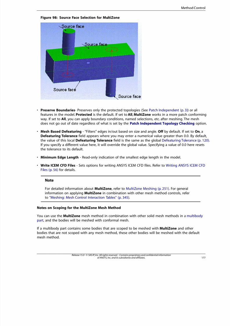
8/10/2019 ANSYS Meshing Users Guide
http://slidepdf.com/reader/full/ansys-meshing-users-guide 185/491
Figure 98: Source Face Selection for MultiZone
• Preserve Boundaries- Preserves only the protected topologies (See Patch Independent (p. 3)) or allfeatures in the model. Protected is the default. If set to All, MultiZone works in a more patch conforming
way. If set to All, you can apply boundary conditions, named selections, etc. after meshing. The meshdoes not go out of date regardless of what is set by the Patch Independent Topology Checking option
• Mesh Based Defeaturing - “Filters” edges in/out based on size and angle. Off by default. If set to On, aDefeaturing Tolerance field appears where you may enter a numerical value greater than 0.0. By defaul
the value of this local Defeaturing Tolerance field is the same as the global Defeaturing Tolerance (p. 12If you specify a different value here, it will override the global value. Specifying a value of 0.0 here resetsthe tolerance to its default.
• Minimum Edge Length - Read-only indication of the smallest edge length in the model.
• Write ICEM CFD Files - Sets options for writing ANSYS ICEM CFD files. Refer to Writing ANSYS ICEM CFDFiles (p. 56) for details.
Note
For detailed information about MultiZone, refer to MultiZone Meshing (p. 251). For general
information on applying MultiZone in combination with other mesh method controls, referto "Meshing: Mesh Control Interaction Tables" (p. 345).
Notes on Scoping for the MultiZone Mesh Method
You can use the MultiZone mesh method in combination with other solid mesh methods in a multibodypart, and the bodies will be meshed with conformal mesh.
If a multibody part contains some bodies that are scoped to be meshed with MultiZone and otherbodies that are not scoped with any mesh method, these other bodies will be meshed with the default
mesh method.
177Release 15.0 - © SAS IP, Inc. All rights reserved. - Contains proprietary and confidential informationof ANSYS, Inc. and its subsidiaries and affiliates.
Method Contro
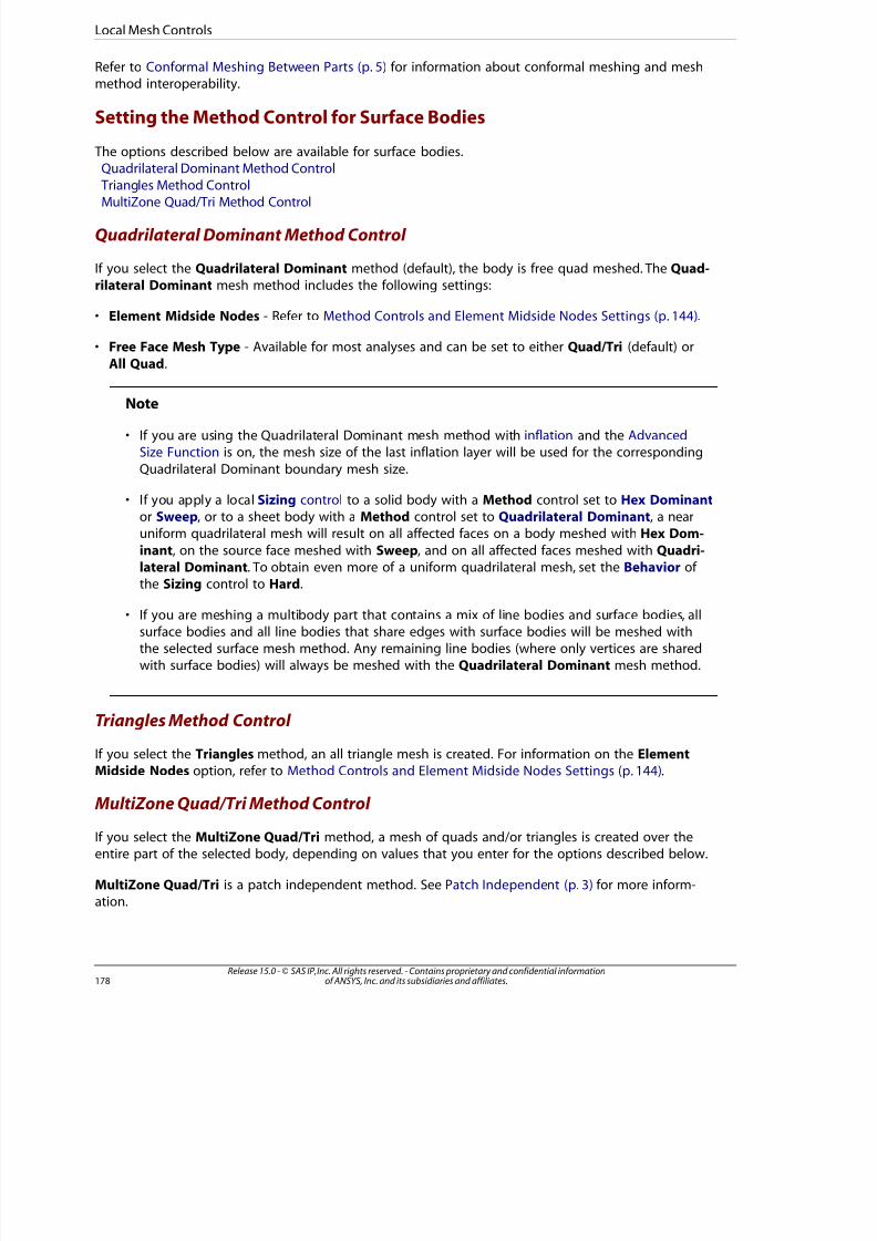
8/10/2019 ANSYS Meshing Users Guide
http://slidepdf.com/reader/full/ansys-meshing-users-guide 186/491
Refer to Conformal Meshing Between Parts (p. 5) for information about conformal meshing and meshmethod interoperability.
Setting the Method Control for Surface Bodies
The options described below are available for surface bodies.Quadrilateral Dominant Method Control Triangles Method ControlMultiZone Quad/Tri Method Control
Quadrilateral Dominant Method Control
If you select the Quadrilateral Dominant method (default), the body is free quad meshed. The Quad-rilateral Dominant mesh method includes the following settings:
• Element Midside Nodes - Refer to Method Controls and Element Midside Nodes Settings (p. 144).
• Free Face Mesh Type - Available for most analyses and can be set to either Quad/Tri (default) or
All Quad.
Note
• If you are using the Quadrilateral Dominant mesh method with inflation and the AdvancedSize Function is on, the mesh size of the last inflation layer will be used for the corresponding
Quadrilateral Dominant boundary mesh size.
• If you apply a local Sizing control to a solid body with a Method control set to Hex Dominantor Sweep, or to a sheet body with a Method control set to Quadrilateral Dominant, a nearuniform quadrilateral mesh will result on all affected faces on a body meshed with Hex Dom-
inant, on the source face meshed with Sweep, and on all affected faces meshed with Quadri-lateral Dominant. To obtain even more of a uniform quadrilateral mesh, set the Behavior of
the Sizing control to Hard.
• If you are meshing a multibody part that contains a mix of line bodies and surface bodies, allsurface bodies and all line bodies that share edges with surface bodies will be meshed withthe selected surface mesh method. Any remaining line bodies (where only vertices are sharedwith surface bodies) will always be meshed with the Quadrilateral Dominant mesh method.
Triangles Method Control
If you select the Triangles method, an all triangle mesh is created. For information on the ElementMidside Nodes option, refer to Method Controls and Element Midside Nodes Settings (p. 144).
MultiZone Quad/Tri Method Control
If you select the MultiZone Quad/Tri method, a mesh of quads and/or triangles is created over theentire part of the selected body, depending on values that you enter for the options described below.
MultiZone Quad/Tri is a patch independent method. See Patch Independent (p. 3) for more inform-ation.
Release 15.0 - © SAS IP, Inc. All rights reserved. - Contains proprietary and confidential informationof ANSYS, Inc. and its subsidiaries and affiliates.178
Local Mesh Controls

8/10/2019 ANSYS Meshing Users Guide
http://slidepdf.com/reader/full/ansys-meshing-users-guide 187/491
Surface Mesh Method - Instructs MultiZone Quad/Tri to use the Program Controlled, Uniform, orPave method to create the mesh.
• Program Controlled - Automatically uses a combination of Uniform and Pave mesh methods de-pending on the mesh sizes set and face properties. This is the default method.
• Uniform - Uses a recursive loop-splitting method which creates a highly uniform mesh. This option
is generally good when all edges have the same sizing and the faces being meshed do not have a
high degree of curvature. The orthogonality of the mesh from this method is generally very good.
• Pave - Uses a paving mesh method which creates a good quality mesh on faces with high curvature,
and also when neighboring edges have a high aspect ratio. This approach is also more reliable togive an all-quad mesh.
Note
The MultiZone Quad/Tri method ignores the Advanced Size Function when Surface MeshMethod is set to Uniform. In such cases, Element Size acts as a hard size.
Note
Models created in versions of ANSYS older than ANSYS 14.5 that have a MultiZone Quad/Trimesh method (previously named Uniform Quad/Tri or Uniform Quad) defined on themwill be resumed in ANSYS 14.5 with the Surface Mesh Method set to Uniform so that themesh is similar to what it was in previous versions. You might want to set the Surface Mesh
Method to Program Controlled for better results.
When resuming these models, the Method control that appears in the Details View will beset to MultiZone Quad/Tri, but the old mesh method name (Uniform Quad/Tri Method or
Uniform Quad Method) will appear in the Tree Outline. To avoid confusion, it may be
helpful to force the software to rename the mesh method object in the Tree Outline. To doso, set Method to a different value (for example, Quadrilateral Dominant) and then resetMethod to MultiZone Quad/Tri. In some cases, you may also see messages containing ref-
erences to the old mesh method names. The names in the messages will be updated to thenew names if/when you remesh.
Element Midside Nodes - Refer to Method Controls and Element Midside Nodes Settings (p. 144).
Free Face Mesh Type - Determines the shape of the mesh elements. Can be All Quad, All Tri, orQuad/Tri (default) for a mesh of pure quad, pure tri, or a combination of quad/tri elements respectively.
Element Size - Allows you to specify the element size used for the selected geometry. Applicable only
when Surface Mesh Method is set to Uniform. Otherwise, uses the global Element Size.
Mesh Based Defeaturing - “Filters” edges in/out based on size and angle. Can be On or Off . By default,this local Mesh Based Defeaturing setting is the same as the setting of the global Automatic MeshBased Defeaturing (p. 120) control. When Mesh Based Defeaturing is On, a Defeaturing Tolerance
field appears where you may enter a numerical value greater than 0.0. By default, the value of this localDefeaturing Tolerance field is the same as the global Defeaturing Tolerance (p. 120). If you specify adifferent value here, it will override the global value. A recommended setting is at least one-half the
179Release 15.0 - © SAS IP, Inc. All rights reserved. - Contains proprietary and confidential informationof ANSYS, Inc. and its subsidiaries and affiliates.
Method Contro

8/10/2019 ANSYS Meshing Users Guide
http://slidepdf.com/reader/full/ansys-meshing-users-guide 188/491
value set for Element Size to assure a successful mesh. Specifying a value of 0.0 here resets the toleranceto its default.
Note
When the global Automatic Mesh Based Defeaturing (p. 120) control is on but the Ad-vanced Size Function is off, the default defeaturing performed for MultiZone Quad/Tri
includes defeaturing based on the dihedral angle between the faces as well as edgelength defeaturing based on the smallest element size set by the user.
Sheet Loop Removal - Removes holes on surface bodies based on size. If set to Yes, a Loop RemovalTolerance field appears where you may enter a numerical value greater than 0.0. By default, the valueof this local Loop Removal Tolerance field is the same as the global Loop Removal Tolerance (p. 120).
If you specify a different value here, it will override the global value. The mesh simply paves over holessmaller than the Loop Removal Tolerance setting.
Minimum Edge Length - Read-only indication of the smallest edge length in the part.
Write ICEM CFD Files - Sets options for writing ANSYS ICEM CFD files. Refer to Writing ANSYS ICEM
CFD Files (p. 56) for details.
Usage Information for the MultiZone Quad/Tri Mesh Method Control
The following usage information is applicable to the MultiZone Quad/Tri mesh method:
• This control is sensitive to the scoping of all other objects in Workbench. If you add a load or support toa group of faces, the part with this mesh method control may need to be remeshed. If you change thescoping of the load, the part may need to be remeshed if the faces or edges are not captured by themesh. The mesh however, is not made obsolete when adding or changing the scoping of a result. It is
recommended that you apply loads to the model before meshing when using this mesh method. SeePatch Independent (p. 3) for more information.
• Base mesh caching is not supported for MultiZone Quad/Tri, so a change to inflation controls requires
remeshing.
• Using MultiZone Quad/Tri may allow meshing over very small bodies in a multibody part. This may leadto a solver error if a body load is associated with that body. If this is the case, you must suppress the bodybefore solving your model.
• Surface bodies with specified variable thickness are not protected topology. To prevent faces and theirboundaries from being meshed over, create an individual Named Selection for each thickness.
• The MultiZone Quad/Tri mesh method supports mesh connections and pinch controls (post pinch only).
• You can use the MultiZone Quad/Tri mesh method in combination with other surface mesh methods ina multibody part, and the bodies will be meshed with conformal mesh. If you select the MultiZoneQuad/Tri mesh method to mesh a multibody part that contains a mix of line bodies and surface bodies,
all surface bodies and all line bodies that share edges with surface bodies will be meshed with the selectedmethod. Any remaining line bodies (where only vertices are shared with surface bodies) will be meshed
Release 15.0 - © SAS IP, Inc. All rights reserved. - Contains proprietary and confidential informationof ANSYS, Inc. and its subsidiaries and affiliates.180
Local Mesh Controls
8/10/2019 ANSYS Meshing Users Guide
http://slidepdf.com/reader/full/ansys-meshing-users-guide 189/491
with the Quadrilateral Dominant mesh method. Refer to Conformal Meshing Between Parts (p. 5) formore information about conformal meshing and mesh method interoperability.
Caution
Multiple environments with different loadings may over-constrain the MultiZone Quad/Trimesher such that the mesher may not be able to return a mesh for the given inputs. If dis-
cretization error is not an issue, the mesher will be less constrained if you duplicate themodel and change the environment instead of adding multiple environments under thesame model.
Mesh Grouping Control
Mesh Grouping identifies bodies that should be grouped together for assembly meshing algorithmsand is available only when assembly meshing algorithms are being used. See Defining MeshGroups (p. 292) for details.
Sizing Control
The sizing control sets:
• The element size for a selected body, face, or edge.
• The number of divisions along an edge.
• The element size within a user-defined “sphere of influence” that can include a selected body, face, edgeor vertex. This control is recommended for local mesh sizing. The control must also be attached to a co-
ordinate system if it is to be scoped to anything other than a vertex.
• The element size within a user-defined “body of influence.” The body of influence will influence the mes
of the body to which it is scoped, but the body of influence itself will not be meshed.
• The minimum mesh sizing used for a selected body, face, or edge. This setting overrides the defaultglobal sizing.
For more information, refer to:Using the Local Sizing Control
Notes on Element Sizing
Using the Local Sizing Control
The basic steps for using the local Sizing control are presented here.
1. Select a body, face, edge, or vertex.
2. From the Mesh Control toolbar, choose Sizing.
or
Right-click on the selected object and choose Insert> Sizing.
18Release 15.0 - © SAS IP, Inc. All rights reserved. - Contains proprietary and confidential informationof ANSYS, Inc. and its subsidiaries and affiliates.
Sizing Contro
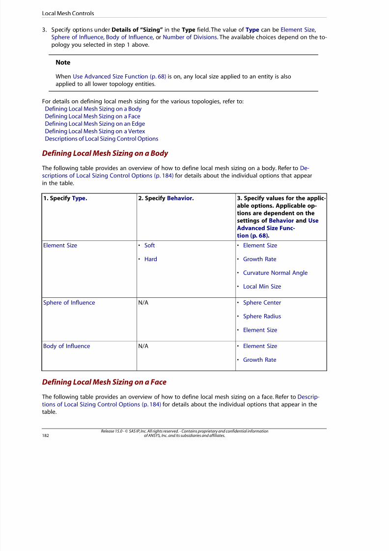
8/10/2019 ANSYS Meshing Users Guide
http://slidepdf.com/reader/full/ansys-meshing-users-guide 190/491
3. Specify options under Details of “Sizing” in the Type field. The value of Type can be Element Size,Sphere of Influence, Body of Influence, or Number of Divisions. The available choices depend on the to-
pology you selected in step 1 above.
Note
When Use Advanced Size Function (p. 68) is on, any local size applied to an entity is also
applied to all lower topology entities.
For details on defining local mesh sizing for the various topologies, refer to:Defining Local Mesh Sizing on a BodyDefining Local Mesh Sizing on a FaceDefining Local Mesh Sizing on an Edge
Defining Local Mesh Sizing on a VertexDescriptions of Local Sizing Control Options
Defining Local Mesh Sizing on a Body
The following table provides an overview of how to define local mesh sizing on a body. Refer to De-scriptions of Local Sizing Control Options (p. 184) for details about the individual options that appear
in the table.
3. Specify values for the applic-
able options. Applicable op-tions are dependent on thesettings of Behavior and Use
Advanced Size Func-tion (p. 68).
2. Specify Behavior.1. Specify Type.
Element Size • Element Size• Soft
• • Growth RateHard
• Curvature Normal Angle
• Local Min Size
N/ASphere of Influence • Sphere Center
• Sphere Radius
• Element Size
N/ABody of Influence • Element Size
• Growth Rate
Defining Local Mesh Sizing on a Face
The following table provides an overview of how to define local mesh sizing on a face. Refer to Descrip-
tions of Local Sizing Control Options (p. 184) for details about the individual options that appear in thetable.
Release 15.0 - © SAS IP, Inc. All rights reserved. - Contains proprietary and confidential informationof ANSYS, Inc. and its subsidiaries and affiliates.182
Local Mesh Controls
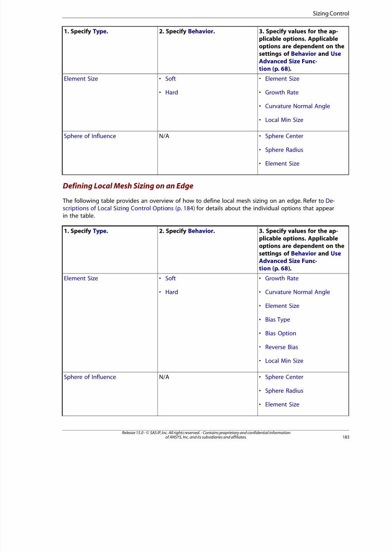
8/10/2019 ANSYS Meshing Users Guide
http://slidepdf.com/reader/full/ansys-meshing-users-guide 191/491
3. Specify values for the ap-plicable options. Applicableoptions are dependent on thesettings of Behavior and Use
Advanced Size Func-tion (p. 68).
2. Specify Behavior.1. Specify Type.
Element Size • Element Size• Soft
• • Growth RateHard
• Curvature Normal Angle
• Local Min Size
N/ASphere of Influence • Sphere Center
• Sphere Radius
• Element Size
Defining Local Mesh Sizing on an Edge
The following table provides an overview of how to define local mesh sizing on an edge. Refer to De-scriptions of Local Sizing Control Options (p. 184) for details about the individual options that appearin the table.
3. Specify values for the ap-plicable options. Applicableoptions are dependent on the
settings of Behavior and Use
Advanced Size Func-tion (p. 68).
2. Specify Behavior.1. Specify Type.
Element Size • Growth Rate• Soft
• • Curvature Normal AngleHard
• Element Size
• Bias Type
• Bias Option
• Reverse Bias
• Local Min Size
N/ASphere of Influence • Sphere Center
• Sphere Radius
• Element Size
183Release 15.0 - © SAS IP, Inc. All rights reserved. - Contains proprietary and confidential informationof ANSYS, Inc. and its subsidiaries and affiliates.
Sizing Contro

8/10/2019 ANSYS Meshing Users Guide
http://slidepdf.com/reader/full/ansys-meshing-users-guide 192/491
3. Specify values for the ap-plicable options. Applicableoptions are dependent on thesettings of Behavior and Use
Advanced Size Func-tion (p. 68).
2. Specify Behavior.1. Specify Type.
Number of Divisions • Growth Rate• Soft
• • Curvature Normal AngleHard
• Number of Divisions
• Bias Type
• Bias Option
• Reverse Bias
Defining Local Mesh Sizing on a Vertex The following table provides an overview of how to define local mesh sizing on a vertex. Refer to De-scriptions of Local Sizing Control Options (p. 184) for details about the individual options that appear
in the table.
2. Specify values for the applicable options.1. Specify Type.
Sphere of Influence • Sphere Radius
• Element Size
Descriptions of Local Sizing Control Options
Use the options described below to further define local mesh sizing. The choices that are available dependon the selected topology, as noted in the individual option descriptions.
Element Size
If you selected a body , face, or edge, Element Size (default) is one of the available options in the Typefield. Enter a positive value (decimals are allowed) in this field. Smaller values generate more divisions.A value of "0" instructs the sizing control to use its defaults.
Additional details about the Element Size option differ depending on whether Use Advanced Size
Function (p. 68) is on or off.
The following series of figures shows the effect of the sizing control applied to a face.
Release 15.0 - © SAS IP, Inc. All rights reserved. - Contains proprietary and confidential informationof ANSYS, Inc. and its subsidiaries and affiliates.184
Local Mesh Controls
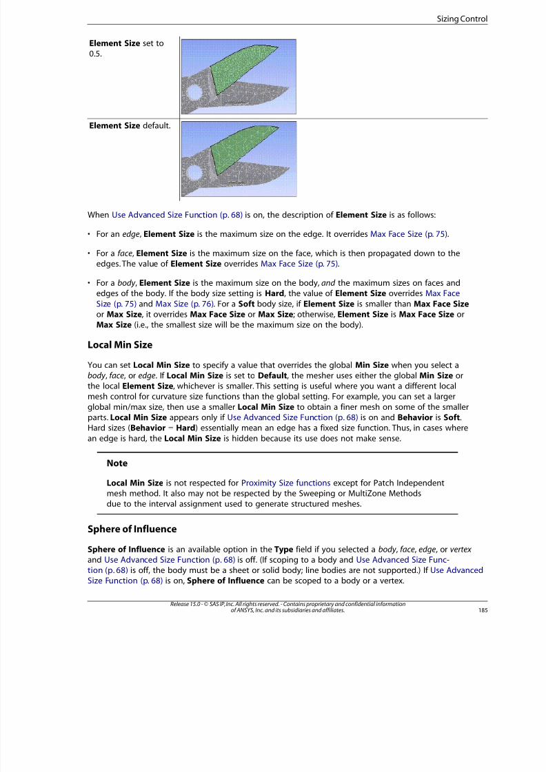
8/10/2019 ANSYS Meshing Users Guide
http://slidepdf.com/reader/full/ansys-meshing-users-guide 193/491
Element Size set to0.5.
Element Size default.
When Use Advanced Size Function (p. 68) is on, the description of Element Size is as follows:
• For an edge, Element Size is the maximum size on the edge. It overrides Max Face Size (p. 75).
• For a face, Element Size is the maximum size on the face, which is then propagated down to theedges. The value of Element Size overrides Max Face Size (p. 75).
• For a body , Element Size is the maximum size on the body, and the maximum sizes on faces andedges of the body. If the body size setting is Hard, the value of Element Size overrides Max Face
Size (p. 75) and Max Size (p. 76). For a Soft body size, if Element Size is smaller than Max Face Sizeor Max Size, it overrides Max Face Size or Max Size; otherwise, Element Size is Max Face Size orMax Size (i.e., the smallest size will be the maximum size on the body).
Local Min Size
You can set Local Min Size to specify a value that overrides the global Min Size when you select abody , face, or edge. If Local Min Size is set to Default, the mesher uses either the global Min Size orthe local Element Size, whichever is smaller. This setting is useful where you want a different localmesh control for curvature size functions than the global setting. For example, you can set a larger
global min/max size, then use a smaller Local Min Size to obtain a finer mesh on some of the smallerparts. Local Min Size appears only if Use Advanced Size Function (p. 68) is on and Behavior is Soft.Hard sizes (Behavior = Hard) essentially mean an edge has a fixed size function. Thus, in cases where
an edge is hard, the Local Min Size is hidden because its use does not make sense.
Note
Local Min Size is not respected for Proximity Size functions except for Patch Independentmesh method. It also may not be respected by the Sweeping or MultiZone Methodsdue to the interval assignment used to generate structured meshes.
Sphere of Influence
Sphere of Influence is an available option in the Type field if you selected a body , face, edge, or vertex
and Use Advanced Size Function (p. 68) is off. (If scoping to a body and Use Advanced Size Func-tion (p. 68) is off, the body must be a sheet or solid body; line bodies are not supported.) If Use AdvancedSize Function (p. 68) is on, Sphere of Influence can be scoped to a body or a vertex.
185Release 15.0 - © SAS IP, Inc. All rights reserved. - Contains proprietary and confidential informationof ANSYS, Inc. and its subsidiaries and affiliates.
Sizing Contro
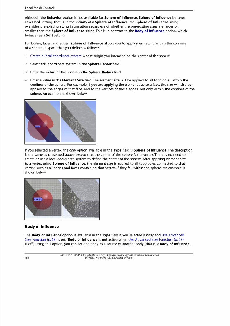
8/10/2019 ANSYS Meshing Users Guide
http://slidepdf.com/reader/full/ansys-meshing-users-guide 194/491
Although the Behavior option is not available for Sphere of Influence, Sphere of Influence behavesas a Hard setting. That is, in the vicinity of a Sphere of Influence, the Sphere of Influence sizing
overrides pre-existing sizing information regardless of whether the pre-existing sizes are larger orsmaller than the Sphere of Influence sizing. This is in contrast to the Body of Influence option, whichbehaves as a Soft setting.
For bodies, faces, and edges, Sphere of Influence allows you to apply mesh sizing within the confinesof a sphere in space that you define as follows:
1. Create a local coordinate system whose origin you intend to be the center of the sphere.
2. Select this coordinate system in the Sphere Center field.
3. Enter the radius of the sphere in the Sphere Radius field.
4. Enter a value in the Element Size field. The element size will be applied to all topologies within the
confines of the sphere. For example, if you are applying the element size to a face, the size will also beapplied to the edges of that face, and to the vertices of those edges, but only within the confines of thesphere. An example is shown below.
If you selected a vertex, the only option available in the Type field is Sphere of Influence. The description
is the same as presented above except that the center of the sphere is the vertex. There is no need tocreate or use a local coordinate system to define the center of the sphere. After applying element sizeto a vertex using Sphere of Influence, the element size is applied to all topologies connected to thatvertex, such as all edges and faces containing that vertex, if they fall within the sphere. An example isshown below.
Body of Influence
The Body of Influence option is available in the Type field if you selected a body and Use AdvancedSize Function (p. 68) is on. (Body of Influence is not active when Use Advanced Size Function (p. 68)is off.) Using this option, you can set one body as a source of another body (that is, a Body of Influence).
Release 15.0 - © SAS IP, Inc. All rights reserved. - Contains proprietary and confidential informationof ANSYS, Inc. and its subsidiaries and affiliates.186
Local Mesh Controls
8/10/2019 ANSYS Meshing Users Guide
http://slidepdf.com/reader/full/ansys-meshing-users-guide 195/491
The Body of Influence will influence the mesh density of the body that it is scoped to, but it will notbe a part of the model geometry nor will it be meshed. Body of Influence bodies are noted in the
Details View of each prototype.
Although the Behavior option is not available for Body of Influence, Body of Influence behaves as aSoft setting. That is, in the vicinity of a Body of Influence, the specified Body of Influence sizing must
be larger than the smallest Min Size (p. 74) /Proximity Min Size (p. 75) and smaller than the global MaxSize (p. 76) to have an effect on the mesh size distribution. The specified Body of Influence sizing im-
poses a local maximum size on all elements that are inside the boundary of the body. This is in contrastto the Sphere of Influence option, which behaves as a Hard setting.
Remember the following notes when using Body of Influence:
• If your source body is a sphere, it is best for you to use the Sphere of Influence option instead of Bodyof Influence. Body of Influence is intended for non-spherical bodies.
• In general, users are discouraged from defining a Body of Influence and a Sphere of Influence such ththe regions of influence overlap. In cases where elements fall within overlapping bodies/spheres of influeelements will be created using the Sphere of Influence sizing that appears lowest in the Tree.
• You cannot apply loads, mesh controls, etc. on bodies of influence. Bodies of influence are used only toinfluence the size function and therefore only size function attributes can be applied to them.
• You can suppress and unsuppress bodies of influence.
• If you are using Body of Influence with Match Control, be aware that the body of influence will not becopied from one matched entity to the other. As a workaround, you can copy the body in the Design-Modeler application and use both bodies as your source.
• When using Assembly Meshing (p. 273), the body of influence cannot be scoped to a line body. If you
want to use a body of influence with a virtual body, you can scope the body of influence to any body inthe geometry. The body of influence does not have to be inside or even in contact with the scoped bod
Although Contact Sizing is supported for assembly meshing algorithms, if it is applied to entities on abody that is scoped to a body of influence, the contact sizing is ignored.
Number of Divisions
Number of Divisions can be used with all meshers except for Assembly Meshing algorithms.
If you select an edge, the options available in the Type field are Element Size and Sphere of Influence,
along with the Number of Divisions option. Choosing Number of Divisions and entering a value inthe Number of Divisions field is an alternative to choosing Element Size if you are interested in havingthe mesh be sized according to a discrete number of divisions along an edge. If you set Number of Divisions to a value greater than 1000, the number of divisions will not be drawn on the edge in the
Geometry window.
Behavior
For bodies, faces, or edges only , you can specify a Behavior option of either Soft (default) or Hard. (TheBehavior option is not available for Sphere of Influence or Body of Influence.) The effect of the Be-
havior setting is influenced by whether Use Advanced Size Function (p. 68) is on or off, as follows:
Regardless of whether Use Advanced Size Function (p. 68) is on or off:
187Release 15.0 - © SAS IP, Inc. All rights reserved. - Contains proprietary and confidential informationof ANSYS, Inc. and its subsidiaries and affiliates.
Sizing Contro

8/10/2019 ANSYS Meshing Users Guide
http://slidepdf.com/reader/full/ansys-meshing-users-guide 196/491
• Choosing the Hard option for edges means that the size or number of divisions is fixed on the edgeand cannot be changed by the meshing algorithm and the likelihood of a mesh failure increases.
• Choosing the Soft option for edges, faces, and bodies means that the size control will be affectedby proximity, curvature, and local remeshing during the meshing process.
If Use Advanced Size Function (p. 68) is off:
• Choosing Hard on a face/body means that curvature pre-refinement is not performed on the edgesof the face/body, but the edge can be split by the mesher.
Interval assignments are handled as follows:
• Regardless of whether Use Advanced Size Function (p. 68) is on or off, choosing Soft on a face/bodymeans that the edges are only seeded with this information in interval assignment; no additionalconstraints are placed on the mesher. A soft constraint in interval assignment places a higher weight
to meet that number of divisions on the edge in the interval solver.
When hard size constraints are placed on faces or bodies that will be swept/mapped, the edgesof those faces/bodies will receive soft edge sizes to guide the interval solver.
Remember these notes when using the Behavior option:
• If Use Advanced Size Function (p. 68) is on and a Soft size is specified on an entity, the specified GrowthRate is used.
If Use Advanced Size Function is on and a Hard size is specified on an entity, the Growth Rate is not
respected; the mesher will try to maintain a uniform size on the entity. If two entities with Hard sizesof different values are adjacent to one another, no growth occurs and there will be an abrupt sizechange between them. However, growth will occur on all entities without hard size constraints that
are adjacent to a hard size entity, even if the Hard size applied is smaller than Min Size /ProximityMin Size.
• If Use Advanced Size Function is on, local size controls take the place of the global max size (Max FaceSize or Max Size, as applicable). TheBehavior option determines how the global Min Size/Proximity
Min Size is used. For example, if a face has a localSoft size defined on it, the local control would be usedin place of the global Max Face Size, however, the min size would still come from the global controls. If instead the face has a local Hard size defined on it, the global min size would be ignored, and the wholeface would be meshed at the size of the local control.
– If the local size control is larger than the global Max Size, the control will be ignored unless the Beha-vior is set to Hard.
• If the Tree contains multiple size controls for the same entity, the last size control for that entity is always
honored.
When Use Advanced Size Function (p. 68) is on, the smallest size that the last size control specifiesfor the entity overrides all other size controls. In this way, the smallest size will be the maximum size
on the entity. This is true unless a Hard size control is used. When size controls are applied to entities
Release 15.0 - © SAS IP, Inc. All rights reserved. - Contains proprietary and confidential informationof ANSYS, Inc. and its subsidiaries and affiliates.188
Local Mesh Controls

8/10/2019 ANSYS Meshing Users Guide
http://slidepdf.com/reader/full/ansys-meshing-users-guide 197/491
of differing dimensions (for example, a face and an edge), a Hard size control will override all othersand the sizing will propagate from the Hard size outward.
Note
For a slender body, specifying Hard local mesh sizing on the body may result in a meshcontaining elements that are much larger than the specified size. To work around this, either
use Soft local mesh sizing on the body instead of Hard sizing, or apply Hard local mesh sizingto the faces of the body.
Growth Rate
You may specify a growth rate for the scoped soft size of an entity (body, face, or edge only ). The descrip-tion of the scoped Growth Rate is the same as that of the global growth rate that you can set in theDetails View when the Mesh object is selected in the Tree Outline. However, the growth rate you specify
for a scoped entity must always be smaller than or equal to the specified global growth rate. GrowthRate is not available for Sphere of Influence. Specifying a growth rate for a face or body affects thegrowth on the face or on the boundary of the body, and its effect continues outside of the scoped entityas well.
Curvature Normal Angle
You may specify Curvature Normal Angle for a scoped entity (body, face, or edge only ). CurvatureNormal Angle is the maximum allowable angle that one element edge is allowed to span. Availableonly when Use Advanced Size Function is set to either On: Proximity and Curvature or On: Curvature.
You can specify a value from 0 to 180 degrees to override the global setting (where a value of 0 resetsthe option to its default). The default for the global setting is calculated based on the values of theRelevance (p. 67) and Span Angle Center (p. 78) options.
Bias Type and Bias Option
For edges only , use Bias Type to adjust the spacing ratio of nodes on an edge. This feature is useful forany engineering problem where nodes need to be clustered on an edge or group of edges, or if thereis a need to bias the mapped mesh of a face towards a specific direction with respect to the edges of the face. Bias Type can be used with all meshers except the Patch Independent Tetrahedron method
and the assembly meshing algorithms. To use Bias Type, choose one of the four pre-determined pat-terned options depicted pictorially from the Bias Type drop down menu:
Note
The MultiZone meshing method respects all Bias Type options. The nodes generally followthe distribution. However, some optimization can be done to improve transition with other
mesh, or to improve the quality. Setting the Behavior to Hard will give higher priority tothe bias settings defined than the optimization.
Then specify a Bias Option. The drop-down menu enables you to choose No Bias, Bias Factor, orSmooth Transition:
189Release 15.0 - © SAS IP, Inc. All rights reserved. - Contains proprietary and confidential informationof ANSYS, Inc. and its subsidiaries and affiliates.
Sizing Contro

8/10/2019 ANSYS Meshing Users Guide
http://slidepdf.com/reader/full/ansys-meshing-users-guide 198/491
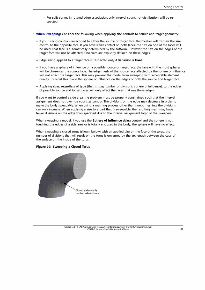
8/10/2019 ANSYS Meshing Users Guide
http://slidepdf.com/reader/full/ansys-meshing-users-guide 199/491
– For split curves in rotated edge association, only interval count, not distribution, will be re-spected.
• When Sweeping: Consider the following when applying size controls to source and target geometry:
– If your sizing controls are scoped to either the source or target face, the mesher will transfer the size
control to the opposite face. If you have a size control on both faces, the size on one of the faces willbe used. That face is automatically determined by the software. However the size on the edges of thetarget face will not be affected if no sizes are explicitly defined on these edges.
– Edge sizing applied to a target face is respected only if Behavior is Hard.
– If you have a sphere of influence on a possible source or target face, the face with the most spheres
will be chosen as the source face. The edge mesh of the source face affected by the sphere of influencwill not affect the target face. This may prevent the model from sweeping with acceptable elementquality. To avoid this, place the sphere of influence on the edges of both the source and target face.
– Applying sizes, regardless of type (that is, size, number of divisions, sphere of influence), to the edges
of possible source and target faces will only affect the faces that use these edges.
If you want to control a side area, the problem must be properly constrained such that the interval
assignment does not override your size control. The divisions on the edge may decrease in order tomake the body sweepable. When using a meshing process other than swept meshing, the divisionscan only increase. When applying a size to a part that is sweepable, the resulting mesh may havefewer divisions on the edge than specified due to the interval assignment logic of the sweepers.
When sweeping a model, if you use the Sphere of Influence sizing control and the sphere is nottouching the edges of a side area or is totally enclosed in the body, the sphere will have no effect.
When sweeping a closed torus (shown below) with an applied size on the face of the torus, the
number of divisions that will result on the torus is governed by the arc length between the caps of the surface on the inside of the torus.
Figure 99: Sweeping a Closed Torus
19Release 15.0 - © SAS IP, Inc. All rights reserved. - Contains proprietary and confidential informationof ANSYS, Inc. and its subsidiaries and affiliates.
Sizing Contro

8/10/2019 ANSYS Meshing Users Guide
http://slidepdf.com/reader/full/ansys-meshing-users-guide 200/491
8/10/2019 ANSYS Meshing Users Guide
http://slidepdf.com/reader/full/ansys-meshing-users-guide 201/491
• If several sizing controls are attached to the same edge, face, or body, the last control is applied. If a sizincontrol is placed on an edge and then another is placed on a face or body that contains that edge, the
edge sizing takes precedence over the face or part sizing.
• If you have adjusted the element size, then changed length units in a CATIA or ACIS model, when youchoose Update or Clear Generated Data at a Model or Project node in the Tree Outline, you may need
to re-adjust the element size. The sizing control does not automatically re-adjust to match this situation.
• When using MultiZone Quad/Tri and Surface Mesh Method is set to Uniform, the Element Size willtake priority over local face or body sizings unless the specified face or body size is smaller than the Ele
Size. This means you can use face or body sizing to obtain a finer mesh, but not to obtain a coarser mes
• When using Assembly Meshing (p. 273):
– The Element Size option for Type is supported for local body, face, and edge sizing. Any bias optionsapplied with edge sizing are ignored.
– The Body of Influence option for Type is supported for local body sizing, but the body of influencecannot be scoped to a line body.
– If you want to use a body of influence with a virtual body, you can scope the body of influence to anybody in the geometry. The body of influence does not have to be inside or even in contact with thescoped body.
– The Sphere of Influence and Number of Divisions options for Type are not supported.
– No local vertex sizing is supported.
– Contact Sizing is supported. However, if contact sizing is applied to entities on a body that is scopedto a body of influence, the contact sizing is ignored.
If any unsupported local size controls are defined prior to selection of an assembly meshing algorithm,
they are suppressed when an assembly meshing algorithm is selected.
• For a table summarizing the behaviors of local sizing controls when used with various mesh methods,refer to Interactions Between Mesh Methods and Mesh Controls (p. 348).
Contact Sizing Control
Contact Sizing creates elements of relatively the same size on bodies from the faces of a face to face
or face to edge contact region. This control generates spheres of influence internally with automaticdetermination of radius and size (if Relevance is selected for Type). You may want to apply a methodcontrol on sweepable bodies to force the elements to be tetrahedron in the case where the sweeperis not providing enough local sizing near your contact region. Your swept mesh may be quite dense if
the contact size is small on the source and target faces of the body. You may also see very little effecton swept bodies in the case where a contact size is applied to a very small region of a large sourceface. You can apply contact sizing using either of the following procedures:
• Choose Contact Sizing from the Mesh Control drop-down menu, or from the context menu through aRMB click on a Mesh object (Insert> Contact Sizing). Select a specific contact region under Scope in thDetails View, then under Type, choose Relevance for a relative size (and enter a value or use the slider),or Element Size (and enter a value) for an absolute size.
193Release 15.0 - © SAS IP, Inc. All rights reserved. - Contains proprietary and confidential informationof ANSYS, Inc. and its subsidiaries and affiliates.
Contact Sizing Contro

8/10/2019 ANSYS Meshing Users Guide
http://slidepdf.com/reader/full/ansys-meshing-users-guide 202/491
• Drag a Contact Region object onto the Mesh object, then in the Details View, under Type, choose Rel-evance for a relative size (and enter a value or use the slider), or Element Size (and enter a value) for an
absolute size.
Note
Since Contact Sizing objects cannot be duplicated, they cannot be used as template objects
for the Object Generator.
Note
Contact sizing works differently for assembly meshing algorithms. See Applying ContactSizing (p. 301) for details.
Refinement Control
Refinement controls specify the maximum number of meshing refinements that are applied to theinitial mesh. Refinement controls are valid for faces, edges, and vertices.
Refinement controls are not available when using the MultiZone, Patch Independent Tetra, or Mul-tiZone Quad/Tri mesh methods, or assembly meshing algorithms. If using MultiZone as part of Auto-
matic mesh method, Refinement behaves similar to the Sweep mesh method.
In the following scenarios, the refinement control is automatically suppressed when used with inflation:
• When automatic inflation (either Program Controlled (p. 81) or All Faces in Chosen Named Selec-
tion (p. 82)) is used with refinement in the same model
• When local inflation is used with refinement in the same body or in the same part
To use refinement controls, click Mesh on the Tree Outline, and right-click to view the menu. SelectInsert> Refinement. You can also click Mesh on the Tree Outline, and select the Mesh Control buttonon the Context Toolbar. Select Refinement.
In the Details View, specify a Refinement number between 1 and 3, where 1 provides minimal refinement,
and 3 provides maximum refinement. If you attach several controls to the same entity, the last controlapplied takes precedence.
Some refinement controls can override or affect other refinements that are on connected topology. Aface refinement control overrides a refinement control on any of the face's edges or vertices. An edge
refinement control overrides a refinement control on either of the edge's vertices. Basically, a refinementcontrol will lower the value of an overridden control by its own value. For example, consider a face with
a refinement control of 1 and one of the face's edges with a refinement control of 2. One of the edge'svertices has a refinement control of 2. In this example, the face control reduces the value of the edge
control by 1. It also reduces the value of the vertex control by 1. The edge control now has a value of 1, so it reduces the vertex's control by 1. Now the vertex has a value of zero, so it has no effect.
Note
• If you apply a Refinement control to a part that was either swept meshed or hex dominant
meshed, then delete the Refinement control, the intermediate tetrahedral mesh will be retained
Release 15.0 - © SAS IP, Inc. All rights reserved. - Contains proprietary and confidential informationof ANSYS, Inc. and its subsidiaries and affiliates.194
Local Mesh Controls
8/10/2019 ANSYS Meshing Users Guide
http://slidepdf.com/reader/full/ansys-meshing-users-guide 203/491
unless you invalidate the state of the part (for example, by clearing the database). An interme-diate tetrahedral mesh is created when you try to refine non-tetrahedral solid elements.
• Refer to Using the Mesh Worksheet to Create a Selective Meshing History (p. 311) for informationabout how refinement operations are processed by the Mesh worksheet.
Mapped Face Meshing Control
Mapped face meshing controls attempt to generate a mapped mesh on selected faces. The Meshingapplication determines a suitable number of divisions for the edges on the boundary face automatically.If you specify the number of divisions on the edge with a Sizing control, the Meshing application at-
tempts to enforce those divisions.
To set the mapped face meshing controls, highlight Mesh in the Tree Outline, and right-click to viewthe menu. Select Insert> Mapped Face Meshing. You can also click Mesh in the Tree Outline, and select
the Mesh Control Context Toolbar, then select Mapped Face Meshing from the drop-down menu.
Note
To assist you in defining mapped face meshing controls, you can use the Show MappableFaces feature to select all mappable faces automatically and highlight them in the Geometrywindow.
There are basic and advanced mapped face meshing controls. Mapped Face Meshing is supported forthe following mesh methods:
Volume Meshing:
• Sweep
• Patch Conforming Tetrahedron
• Hex Dominant
• MultiZone (basic controls only)
Surface Meshing:
• Quadrilateral Dominant
• Triangles
• MultiZone Quad/Tri (basic controls only)
Mapped face meshing topics include:
Setting Basic Mapped Face Meshing ControlsUnderstanding Advanced Mapped Face Meshing Controls
195Release 15.0 - © SAS IP, Inc. All rights reserved. - Contains proprietary and confidential informationof ANSYS, Inc. and its subsidiaries and affiliates.
Mapped Face Meshing Contro
8/10/2019 ANSYS Meshing Users Guide
http://slidepdf.com/reader/full/ansys-meshing-users-guide 204/491
Notes on the Mapped Face Meshing Control
Note
For general information on applying mapped face meshing controls in combination with the
various mesh method controls, refer to "Meshing: Mesh Control Interaction Tables" (p. 345).
Setting Basic Mapped Face Meshing Controls
This section describes the steps for setting basic mapped face meshing controls.
To set basic mapped face meshing controls:
1. Insert a mapped face meshing control by highlighting Mesh in the Tree and right-clicking to view the
menu. Select Insert> Mapped Face Meshing.
2. Select the face that you want to be mapped meshed.
3. For the Definition> Method control, choose Quadrilaterals or Triangles: Best Split. (The Triangles:
Best Split option is available only for sheet models.)
4. For the Definition> Internal Number of Divisions control, specify the number of divisions across an-nular regions or seamless cylinders. (The Internal Number of Divisions option is activated when theMapped Face Meshing control is scoped to faces made up of two loops.) The default value is 0.
5. For the Definition> Constrain Boundary control, specify whether you want to allow the mesher tosplit the boundary of a mapped mesh region to aid in meshing of adjacent faces. You can choose Yes(constrain boundary; no splitting is allowed) or No (do not constrain boundary; splitting is allowed).
The default is No. See Notes on the Mapped Face Meshing Control (p. 202) for related information.
6. Generate the mesh by right-clicking the Mesh object in the Tree and selecting Generate Mesh.
Understanding Advanced Mapped Face Meshing Controls
When you apply advanced mapped face meshing controls to a face, the Meshing application dividesthe face into one or more mappable regions and creates a mapped mesh in each region. Advanced
mapped face meshing controls are subject to restrictions related to vertex types and restrictions relatedto edge mesh intervals.
The advanced Mapped Face Meshing controls are supported for the following mesh methods only:
Volume Meshing:
• Sweep
• Patch Conforming Tetrahedron
• Hex Dominant
Surface Meshing:
• Quadrilateral Dominant
• Triangles
Release 15.0 - © SAS IP, Inc. All rights reserved. - Contains proprietary and confidential informationof ANSYS, Inc. and its subsidiaries and affiliates.196
Local Mesh Controls
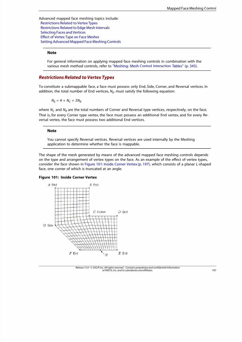
8/10/2019 ANSYS Meshing Users Guide
http://slidepdf.com/reader/full/ansys-meshing-users-guide 205/491
Advanced mapped face meshing topics include:Restrictions Related to Vertex Types
Restrictions Related to Edge Mesh IntervalsSelecting Faces and VerticesEffect of Vertex Type on Face Meshes
Setting Advanced Mapped Face Meshing Controls
Note
For general information on applying mapped face meshing controls in combination with thevarious mesh method controls, refer to "Meshing: Mesh Control Interaction Tables" (p. 345).
Restrictions Related to Vertex Types
To constitute a submappable face, a face must possess only End, Side, Corner, and Reversal vertices. In
addition, the total number of End vertices, N E , must satisfy the following equation:
N E = 4 + N C + 2N R
where N C and N R are the total numbers of Corner and Reversal type vertices, respectively, on the face.
That is, for every Corner type vertex, the face must possess an additional End vertex, and for every Re-
versal vertex, the face must possess two additional End vertices.
Note
You cannot specify Reversal vertices. Reversal vertices are used internally by the Meshingapplication to determine whether the face is mappable.
The shape of the mesh generated by means of the advanced mapped face meshing controls depends
on the type and arrangement of vertex types on the face. As an example of the effect of vertex types,consider the face shown in Figure 101: Inside Corner Vertex (p. 197), which consists of a planar L-shapedface, one corner of which is truncated at an angle.
Figure 101: Inside Corner Vertex
197Release 15.0 - © SAS IP, Inc. All rights reserved. - Contains proprietary and confidential informationof ANSYS, Inc. and its subsidiaries and affiliates.
Mapped Face Meshing Contro
8/10/2019 ANSYS Meshing Users Guide
http://slidepdf.com/reader/full/ansys-meshing-users-guide 206/491
In Figure 101: Inside Corner Vertex (p. 197), the inside corner vertex (C ) is designated as a Corner vertex,therefore, in order to be submappable, the face must possess five End type vertices ( A, B, D, E , and F ).
The advanced mapped face mesh control divides the face into the following two mapped regions:
• A, B, C , H , F , G
• C , D, E , H
Note
If you enforce an advanced mapped face mesh control on a face, the Meshing applicationevaluates the face with respect to its vertex type designations. If the vertex types do notmeet the criteria outlined above, the Meshing application attempts to change the vertex
types so that the face is submappable.
For most submappable faces, there are multiple configurations of vertex types that satisfythe vertex type criteria. Each vertex type configuration results in a unique node pattern forthe submapped mesh. When the Meshing application automatically changes vertex types,
it attempts to employ the configuration that minimizes distortion in the mesh. To enforce a
specific node pattern on a submapped mesh, manually select the vertices such that theymeet the advanced mapped mesh control vertex type criteria outlined above. (See Selecting
the Vertex Type and Picking Vertices (p. 198).)
Restrictions Related to Edge Mesh Intervals
If you specify a bias on the edge of a face before applying an advanced mapped face mesh control tothe face, you must specify the bias on all parallel edges of the face.
Selecting Faces and Vertices
To use advanced mapped mesh controls on a face, you must do the following:
• Select the face upon which the vertex types are to be defined
• Select the vertex type (using the Specified Sides, Specified Corners, and Specified Ends controls)
• Pick the vertices to which the vertex type specification is to be applied
Selecting the Face
The Meshing application vertex types are specific to the faces upon which they are set. Therefore, to
specify the type designation of an individual vertex, you must first select a face to be associated withthat vertex. An individual vertex may possess as many vertex type designations as the number of faces
to which it is attached. For example, it is possible for a vertex to possess a Side type designation withrespect to one face and an End type designation with respect to another, as long as two separateMapped Face Meshing controls are defined for the two faces. For more information, refer to SettingAdvanced Mapped Face Meshing Controls (p. 201).
Selecting the Vertex Type and Picking Vertices
The structure of any face mesh in the vicinity of an individual vertex on its boundary is a function of
the vertex type. There are three vertex types that you can specify.
Release 15.0 - © SAS IP, Inc. All rights reserved. - Contains proprietary and confidential informationof ANSYS, Inc. and its subsidiaries and affiliates.198
Local Mesh Controls
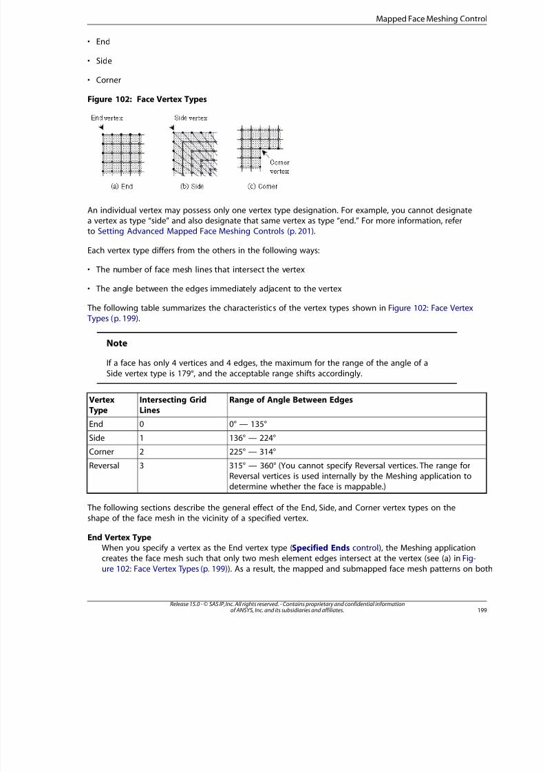
8/10/2019 ANSYS Meshing Users Guide
http://slidepdf.com/reader/full/ansys-meshing-users-guide 207/491
• End
• Side
• Corner
Figure 102: Face Vertex Types
An individual vertex may possess only one vertex type designation. For example, you cannot designatea vertex as type “side” and also designate that same vertex as type “end.” For more information, referto Setting Advanced Mapped Face Meshing Controls (p. 201).
Each vertex type differs from the others in the following ways:
• The number of face mesh lines that intersect the vertex
• The angle between the edges immediately adjacent to the vertex
The following table summarizes the characteristics of the vertex types shown in Figure 102: Face Vertex Types (p. 199).
Note
If a face has only 4 vertices and 4 edges, the maximum for the range of the angle of aSide vertex type is 179°, and the acceptable range shifts accordingly.
Range of Angle Between EdgesIntersecting GridLines
VertexType
0° — 135°0End
136° — 224°1Side
225° — 314°2Corner
315° — 360° (You cannot specify Reversal vertices. The range forReversal vertices is used internally by the Meshing application to
determine whether the face is mappable.)
3Reversal
The following sections describe the general effect of the End, Side, and Corner vertex types on theshape of the face mesh in the vicinity of a specified vertex.
End Vertex TypeWhen you specify a vertex as the End vertex type (Specified Ends control), the Meshing applicationcreates the face mesh such that only two mesh element edges intersect at the vertex (see (a) in Fig-
ure 102: Face Vertex Types (p. 199)). As a result, the mapped and submapped face mesh patterns on bo
199Release 15.0 - © SAS IP, Inc. All rights reserved. - Contains proprietary and confidential informationof ANSYS, Inc. and its subsidiaries and affiliates.
Mapped Face Meshing Contro
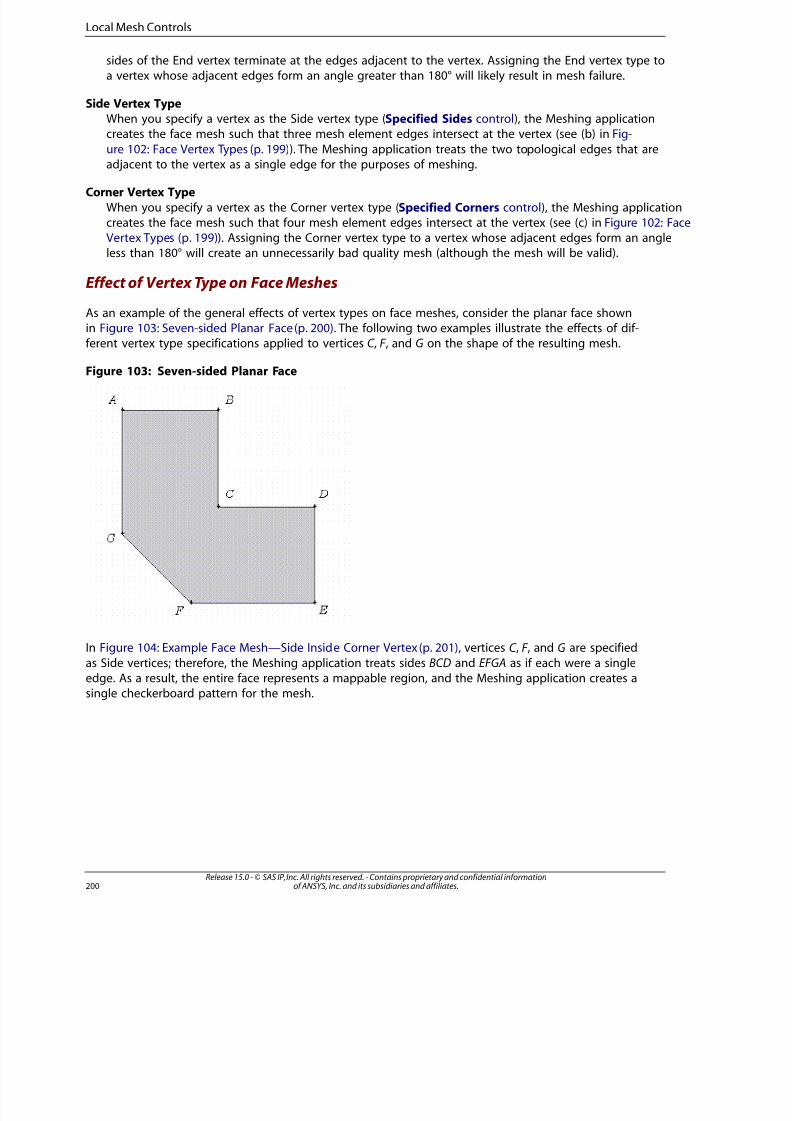
8/10/2019 ANSYS Meshing Users Guide
http://slidepdf.com/reader/full/ansys-meshing-users-guide 208/491
sides of the End vertex terminate at the edges adjacent to the vertex. Assigning the End vertex type toa vertex whose adjacent edges form an angle greater than 180° will likely result in mesh failure.
Side Vertex TypeWhen you specify a vertex as the Side vertex type (Specified Sides control), the Meshing applicationcreates the face mesh such that three mesh element edges intersect at the vertex (see (b) in Fig-
ure 102: Face Vertex Types (p. 199)). The Meshing application treats the two topological edges that areadjacent to the vertex as a single edge for the purposes of meshing.
Corner Vertex Type
When you specify a vertex as the Corner vertex type (Specified Corners control), the Meshing applicationcreates the face mesh such that four mesh element edges intersect at the vertex (see (c) in Figure 102: FaceVertex Types (p. 199)). Assigning the Corner vertex type to a vertex whose adjacent edges form an angleless than 180° will create an unnecessarily bad quality mesh (although the mesh will be valid).
Effect of Vertex Type on Face Meshes
As an example of the general effects of vertex types on face meshes, consider the planar face shownin Figure 103: Seven-sided Planar Face (p. 200). The following two examples illustrate the effects of dif-ferent vertex type specifications applied to vertices C , F , and G on the shape of the resulting mesh.
Figure 103: Seven-sided Planar Face
In Figure 104: Example Face Mesh—Side Inside Corner Vertex (p. 201), vertices C , F , and G are specified
as Side vertices; therefore, the Meshing application treats sides BCD and EFGA as if each were a singleedge. As a result, the entire face represents a mappable region, and the Meshing application creates asingle checkerboard pattern for the mesh.
Release 15.0 - © SAS IP, Inc. All rights reserved. - Contains proprietary and confidential informationof ANSYS, Inc. and its subsidiaries and affiliates.200
Local Mesh Controls
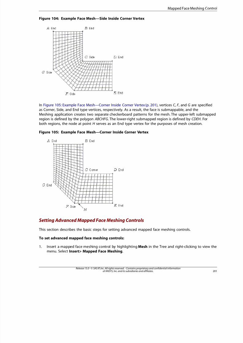
8/10/2019 ANSYS Meshing Users Guide
http://slidepdf.com/reader/full/ansys-meshing-users-guide 209/491
Figure 104: Example Face Mesh—Side Inside Corner Vertex
In Figure 105: Example Face Mesh—Corner Inside Corner Vertex (p. 201), vertices C , F , and G are specifiedas Corner, Side, and End type vertices, respectively. As a result, the face is submappable, and the
Meshing application creates two separate checkerboard patterns for the mesh. The upper-left submappedregion is defined by the polygon ABCHFG. The lower-right submapped region is defined by CDEH . Forboth regions, the node at point H serves as an End type vertex for the purposes of mesh creation.
Figure 105: Example Face Mesh—Corner Inside Corner Vertex
Setting Advanced Mapped Face Meshing Controls
This section describes the basic steps for setting advanced mapped face meshing controls.
To set advanced mapped face meshing controls:
1. Insert a mapped face meshing control by highlighting Mesh in the Tree and right-clicking to view themenu. Select Insert> Mapped Face Meshing.
20Release 15.0 - © SAS IP, Inc. All rights reserved. - Contains proprietary and confidential informationof ANSYS, Inc. and its subsidiaries and affiliates.
Mapped Face Meshing Contro
8/10/2019 ANSYS Meshing Users Guide
http://slidepdf.com/reader/full/ansys-meshing-users-guide 210/491
2. Select the face upon which the vertex types are to be defined by scoping the face in the Mapped FaceMeshing Details View. (Refer to Selecting the Face (p. 198) for more information.)
3. For the Definition> Method control, choose Quadrilaterals or Triangles: Best Split.
4. Enter additional Definition settings, as desired, in the Details View.
5. Use the Specified Sides, Specified Corners, and Specified Ends controls in the Advanced section of
the Details View to select the desired vertices in the Geometry window and apply your selections. Todo so, pick the desired vertex/vertices in the Geometry window and then click on the Specified Sides,Specified Corners, or Specified Ends control to assign the vertex/vertices to the desired vertex type.
(Refer to Selecting the Vertex Type and Picking Vertices (p. 198) for more information.)
Note
If you select a vertex by mistake and want to de-select it, click the control in questionin the Advanced section of the Details View, clear the selection by clicking in an “empty”portion of the Geometry window, and then click Apply. For example, assume that you
mistakenly selected 1 vertex for the Specified Corners control. To clear the selection:
• In the Specified Corners control in the Advanced section of the Details View, click on your selection (that is, the text “1 Vertex”).
The Apply /Cancel buttons will appear in the Specified Corners control and thevertex will be highlighted in green in the Geometry window.
• Click in an empty portion of the Geometry window.
• Click Apply in the Specified Corners control.
Note
An individual vertex may possess as many vertex type designations as the number of faces to which it is attached. For example, it is possible for a vertex to possess a Sidetype designation with respect to one face and an End type designation with respect to
another, as long as two separate Mapped Face Meshing controls are defined for thetwo faces. Conversely, a single Mapped Face Meshing control cannot specify the samevertex as more than one vertex type. That is, you cannot designate a vertex as type Sideand also designate that same vertex as type End in a single Mapped Face Meshing
control. If you attempt to do so, the second and any subsequent assignments for thatvertex will result in the control being highlighted in yellow in the Advanced section of the Details View, and you will not be able to generate a mesh. If this occurs, use the
procedure noted above to de-select the unwanted vertex assignment(s).
6. Generate the mesh by right-clicking the Mesh object in the Tree and selecting Generate Mesh.
Notes on the Mapped Face Meshing Control
Remember the following notes when using the Mapped Face Meshing control:
Release 15.0 - © SAS IP, Inc. All rights reserved. - Contains proprietary and confidential informationof ANSYS, Inc. and its subsidiaries and affiliates.202
Local Mesh Controls
8/10/2019 ANSYS Meshing Users Guide
http://slidepdf.com/reader/full/ansys-meshing-users-guide 211/491
• The blue status icon that may appear in the Tree Outline indicates that a mapped mesh cannot be provion the scoped topology. One of three scenarios triggers the icon:
1. The face cannot be map meshed.
2. The quality of the mapped mesh was not acceptable and a free mesh was generated.
3. If Constrain Boundary is set to Yes, the mesher will fail if the boundary of a mapped mesh needs to
be modified.
• To assist you in working with Mapped Face Meshing, you may want to use the Show Mappable Faces,Show Sweepable Bodies, and/or Preview Surface Mesh features. The Show Mappable Faces feature
selects all mappable faces automatically and highlights them in the Geometry window. By using theShow Sweepable Bodies feature, you can find out whether bodies are sweepable (before and aftermodifying vertex types). By using the Preview Surface Mesh feature, you can verify that your mesh settare correct.
• When sweeping:
– If the sweep method is applied to a body and a Mapped Face Meshing control is defined for either
the body's source or target face, the sweep mesher will fail if a mapped mesh cannot be obtained forthe face.
– When a side face has a Mapped Face Meshing control, the mapped mesher will loosen its toleranceson determining whether a face is mappable.
– When sweeping and using advanced mapped meshing controls, you must set vertex types for both thsource and target faces.
• When a face has only 4 vertices and 4 edges, and a Mapped Face Meshing control is applied, the only
factor that will determine a successful mapped mesh is element quality.
Note
It is often helpful to use the Show Vertices option to ensure edges are complete and donot have unintended segmentation. If an edge is segmented, it could mean that a faceyou think should be successfully mapped actually has 5 vertices and 5 edges. To help resolve
such issues, you can define a virtual edge or use advanced mapped meshing controls.
• An effective technique for mapped meshing on surface bodies is to select all faces on the body and letthe mesher determine which faces should be map meshed and which faces should be free meshed.
• The Mapped Face Meshing control is not supported for assembly meshing algorithms.
• If the Mapped Face Meshing control is attached to faces with exactly two boundary edges or two setsof boundary edges, an additional option, Internal Number of Divisions, is available. This option allowsyou to specify the number of layers of elements that will be generated between the two boundary edge
– If there is a conflict between Internal Number of Divisions and a Face sizing control, the mappedface control's Internal Number of Divisions value will take priority.
– If there is a conflict between Internal Number of Divisions and a parallel Edge sizing control, the
Sweep mesh method will respect the Internal Number of Divisions unless the size is hard, in which cas
203Release 15.0 - © SAS IP, Inc. All rights reserved. - Contains proprietary and confidential informationof ANSYS, Inc. and its subsidiaries and affiliates.
Mapped Face Meshing Contro
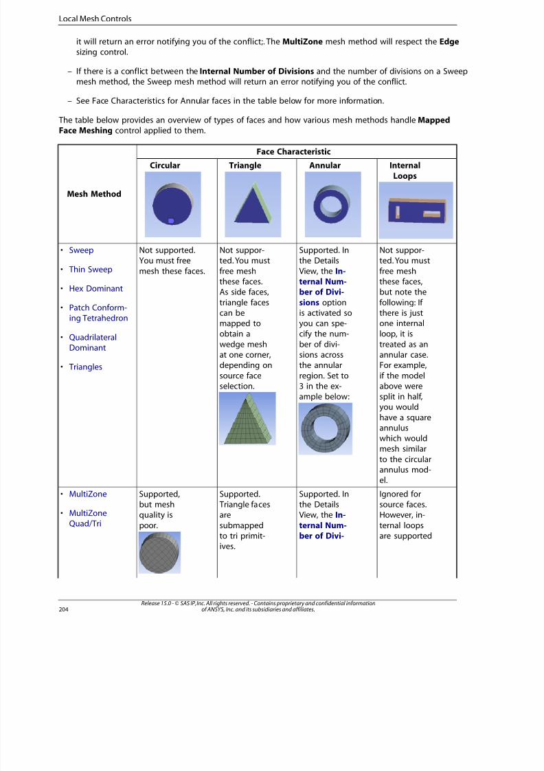
8/10/2019 ANSYS Meshing Users Guide
http://slidepdf.com/reader/full/ansys-meshing-users-guide 212/491
it will return an error notifying you of the conflict;. The MultiZone mesh method will respect the Edgesizing control.
– If there is a conflict between the Internal Number of Divisions and the number of divisions on a Sweepmesh method, the Sweep mesh method will return an error notifying you of the conflict.
– See Face Characteristics for Annular faces in the table below for more information.
The table below provides an overview of types of faces and how various mesh methods handle MappedFace Meshing control applied to them.
Face Characteristic
Mesh Method
Internal
Loops
AnnularTriangleCircular
Not suppor-ted. You must
Supported. Inthe Details
Not suppor-ted. You must
Not supported.You must free
mesh these faces.
• Sweep
• Thin Sweep free meshthese faces,
View, the In-ternal Num-
free meshthese faces.
• Hex Dominant but note theber of Divi-As side faces,
following: If sions optiontriangle faces• Patch Conform-
ing Tetrahedronthere is justone internal
is activated soyou can spe-
can bemapped to
loop, it iscify the num-obtain a• QuadrilateralDominant treated as an
annular case.ber of divi-sions across
wedge meshat one corner,
For example,the annulardepending on• Trianglesif the modelregion. Set tosource face
selection. above were3 in the ex-ample below: split in half,
you would
have a squareannuluswhich wouldmesh similar
to the circularannulus mod-
el.Ignored forsource faces.
Supported. Inthe Details
Supported. Triangle faces
Supported,but mesh
• MultiZone
• MultiZoneQuad/Tri
However, in-
ternal loopsare supported
View, the In-
ternal Num-ber of Divi-
are
submappedto tri primit-ives.
quality is
poor.
Release 15.0 - © SAS IP, Inc. All rights reserved. - Contains proprietary and confidential informationof ANSYS, Inc. and its subsidiaries and affiliates.204
Local Mesh Controls
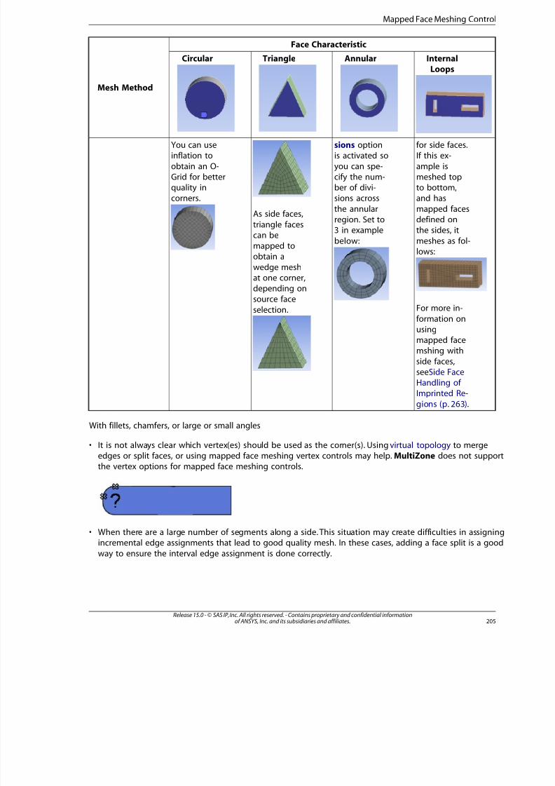
8/10/2019 ANSYS Meshing Users Guide
http://slidepdf.com/reader/full/ansys-meshing-users-guide 213/491
Face Characteristic
Mesh Method
InternalLoops
AnnularTriangleCircular
You can useinflation to
for side faces.If this ex-
sions optionis activated so
As side faces,
triangle faces
obtain an O-Grid for betterquality incorners.
ample ismeshed topto bottom,and has
mapped facesdefined onthe sides, it
meshes as fol-lows:
you can spe-cify the num-ber of divi-sions across
the annularregion. Set to3 in example
below:can be
mapped toobtain a
wedge meshat one corner,depending onsource face
selection. For more in-
formation onusingmapped facemshing with
side faces,
seeSide FaceHandling of Imprinted Re-
gions (p. 263).
With fillets, chamfers, or large or small angles
• It is not always clear which vertex(es) should be used as the corner(s). Using virtual topology to mergeedges or split faces, or using mapped face meshing vertex controls may help. MultiZone does not suppothe vertex options for mapped face meshing controls.
• When there are a large number of segments along a side. This situation may create difficulties in assigniincremental edge assignments that lead to good quality mesh. In these cases, adding a face split is a goo
way to ensure the interval edge assignment is done correctly.
205Release 15.0 - © SAS IP, Inc. All rights reserved. - Contains proprietary and confidential informationof ANSYS, Inc. and its subsidiaries and affiliates.
Mapped Face Meshing Contro
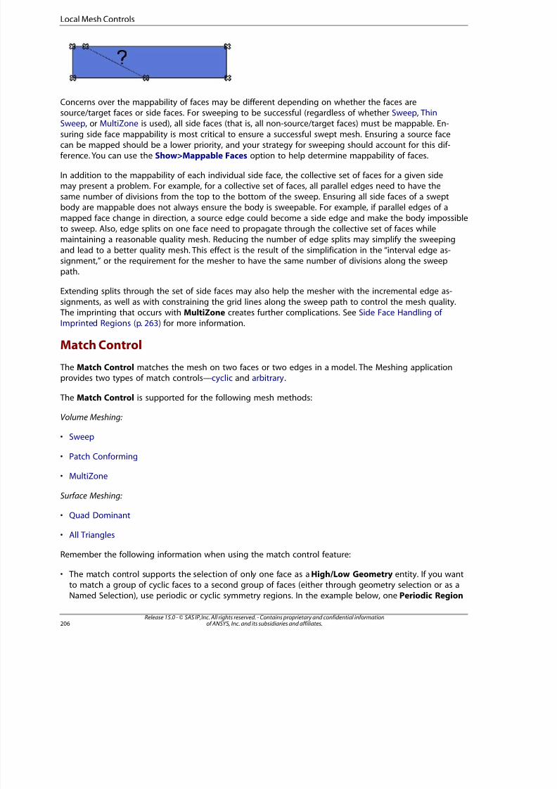
8/10/2019 ANSYS Meshing Users Guide
http://slidepdf.com/reader/full/ansys-meshing-users-guide 214/491
Concerns over the mappability of faces may be different depending on whether the faces aresource/target faces or side faces. For sweeping to be successful (regardless of whether Sweep, Thin
Sweep, or MultiZone is used), all side faces (that is, all non-source/target faces) must be mappable. En-suring side face mappability is most critical to ensure a successful swept mesh. Ensuring a source facecan be mapped should be a lower priority, and your strategy for sweeping should account for this dif-ference. You can use the Show>Mappable Faces option to help determine mappability of faces.
In addition to the mappability of each individual side face, the collective set of faces for a given sidemay present a problem. For example, for a collective set of faces, all parallel edges need to have thesame number of divisions from the top to the bottom of the sweep. Ensuring all side faces of a sweptbody are mappable does not always ensure the body is sweepable. For example, if parallel edges of a
mapped face change in direction, a source edge could become a side edge and make the body impossibleto sweep. Also, edge splits on one face need to propagate through the collective set of faces whilemaintaining a reasonable quality mesh. Reducing the number of edge splits may simplify the sweeping
and lead to a better quality mesh. This effect is the result of the simplification in the “interval edge as-signment,” or the requirement for the mesher to have the same number of divisions along the sweeppath.
Extending splits through the set of side faces may also help the mesher with the incremental edge as-
signments, as well as with constraining the grid lines along the sweep path to control the mesh quality. The imprinting that occurs with MultiZone creates further complications. See Side Face Handling of Imprinted Regions (p. 263) for more information.
Match Control
The Match Control matches the mesh on two faces or two edges in a model. The Meshing applicationprovides two types of match controls—cyclic and arbitrary.
The Match Control is supported for the following mesh methods:
Volume Meshing:
• Sweep
• Patch Conforming
• MultiZone
Surface Meshing:
• Quad Dominant
• All Triangles
Remember the following information when using the match control feature:
• The match control supports the selection of only one face as a High/Low Geometry entity. If you wantto match a group of cyclic faces to a second group of faces (either through geometry selection or as aNamed Selection), use periodic or cyclic symmetry regions. In the example below, one Periodic Region
Release 15.0 - © SAS IP, Inc. All rights reserved. - Contains proprietary and confidential informationof ANSYS, Inc. and its subsidiaries and affiliates.206
Local Mesh Controls
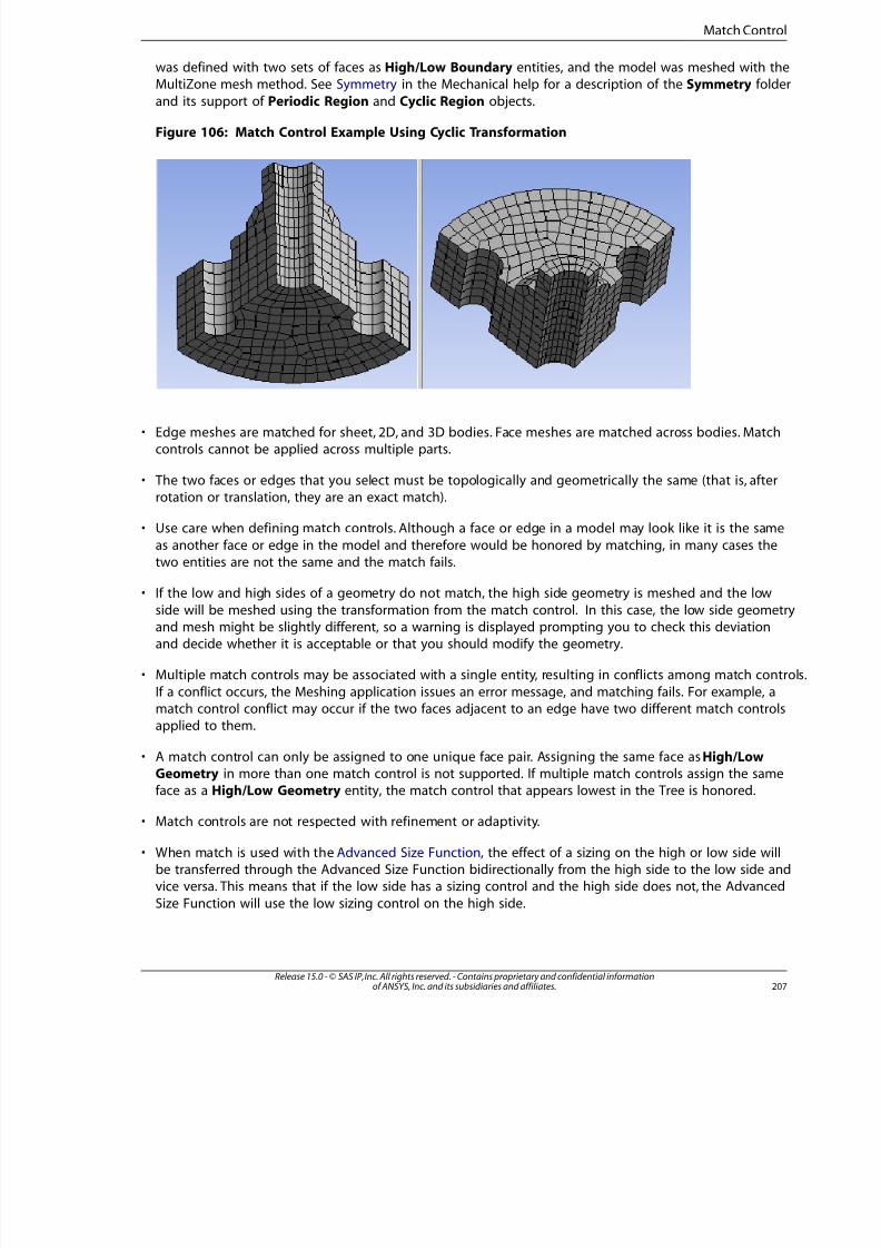
8/10/2019 ANSYS Meshing Users Guide
http://slidepdf.com/reader/full/ansys-meshing-users-guide 215/491
was defined with two sets of faces as High/Low Boundary entities, and the model was meshed with theMultiZone mesh method. See Symmetry in the Mechanical help for a description of the Symmetry folde
and its support of Periodic Region and Cyclic Region objects.
Figure 106: Match Control Example Using Cyclic Transformation
• Edge meshes are matched for sheet, 2D, and 3D bodies. Face meshes are matched across bodies. Matchcontrols cannot be applied across multiple parts.
• The two faces or edges that you select must be topologically and geometrically the same (that is, afterrotation or translation, they are an exact match).
• Use care when defining match controls. Although a face or edge in a model may look like it is the same
as another face or edge in the model and therefore would be honored by matching, in many cases thetwo entities are not the same and the match fails.
• If the low and high sides of a geometry do not match, the high side geometry is meshed and the lowside will be meshed using the transformation from the match control. In this case, the low side geometand mesh might be slightly different, so a warning is displayed prompting you to check this deviationand decide whether it is acceptable or that you should modify the geometry.
• Multiple match controls may be associated with a single entity, resulting in conflicts among match contr
If a conflict occurs, the Meshing application issues an error message, and matching fails. For example, amatch control conflict may occur if the two faces adjacent to an edge have two different match controlsapplied to them.
• A match control can only be assigned to one unique face pair. Assigning the same face as High/LowGeometry in more than one match control is not supported. If multiple match controls assign the sameface as a High/Low Geometry entity, the match control that appears lowest in the Tree is honored.
• Match controls are not respected with refinement or adaptivity.
• When match is used with the Advanced Size Function, the effect of a sizing on the high or low side willbe transferred through the Advanced Size Function bidirectionally from the high side to the low side andvice versa. This means that if the low side has a sizing control and the high side does not, the Advanced
Size Function will use the low sizing control on the high side.
207Release 15.0 - © SAS IP, Inc. All rights reserved. - Contains proprietary and confidential informationof ANSYS, Inc. and its subsidiaries and affiliates.
Match Contro
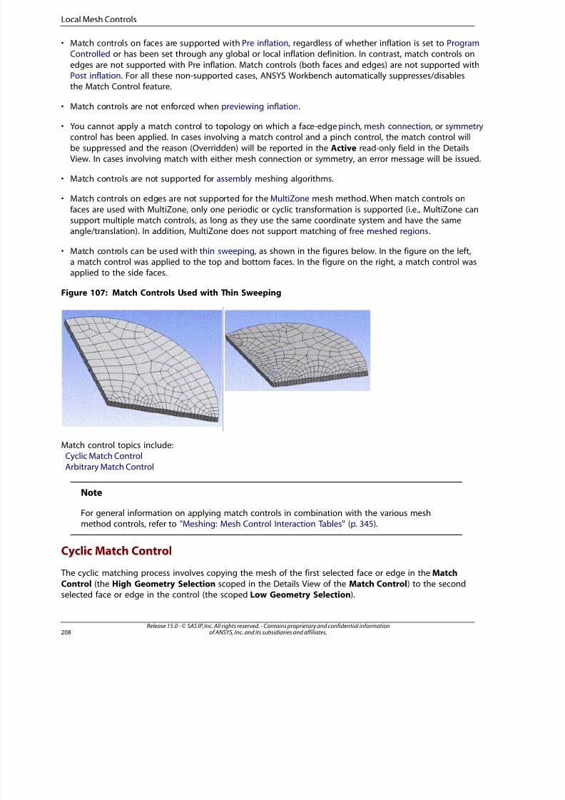
8/10/2019 ANSYS Meshing Users Guide
http://slidepdf.com/reader/full/ansys-meshing-users-guide 216/491
• Match controls on faces are supported with Pre inflation, regardless of whether inflation is set to ProgramControlled or has been set through any global or local inflation definition. In contrast, match controls on
edges are not supported with Pre inflation. Match controls (both faces and edges) are not supported withPost inflation. For all these non-supported cases, ANSYS Workbench automatically suppresses/disablesthe Match Control feature.
• Match controls are not enforced when previewing inflation.
• You cannot apply a match control to topology on which a face-edge pinch, mesh connection, or symmetrycontrol has been applied. In cases involving a match control and a pinch control, the match control will
be suppressed and the reason (Overridden) will be reported in the Active read-only field in the DetailsView. In cases involving match with either mesh connection or symmetry, an error message will be issued.
• Match controls are not supported for assembly meshing algorithms.
• Match controls on edges are not supported for the MultiZone mesh method. When match controls on
faces are used with MultiZone, only one periodic or cyclic transformation is supported (i.e., MultiZone cansupport multiple match controls, as long as they use the same coordinate system and have the sameangle/translation). In addition, MultiZone does not support matching of free meshed regions.
• Match controls can be used with thin sweeping, as shown in the figures below. In the figure on the left,a match control was applied to the top and bottom faces. In the figure on the right, a match control wasapplied to the side faces.
Figure 107: Match Controls Used with Thin Sweeping
Match control topics include:Cyclic Match Control
Arbitrary Match Control
Note
For general information on applying match controls in combination with the various meshmethod controls, refer to "Meshing: Mesh Control Interaction Tables" (p. 345).
Cyclic Match Control
The cyclic matching process involves copying the mesh of the first selected face or edge in the Match
Control (the High Geometry Selection scoped in the Details View of the Match Control) to the secondselected face or edge in the control (the scoped Low Geometry Selection).
Release 15.0 - © SAS IP, Inc. All rights reserved. - Contains proprietary and confidential informationof ANSYS, Inc. and its subsidiaries and affiliates.208
Local Mesh Controls
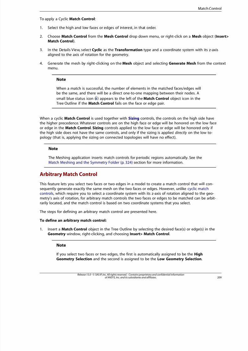
8/10/2019 ANSYS Meshing Users Guide
http://slidepdf.com/reader/full/ansys-meshing-users-guide 217/491
To apply a Cyclic Match Control:
1. Select the high and low faces or edges of interest, in that order.
2. Choose Match Control from the Mesh Control drop down menu, or right-click on a Mesh object (InsMatch Control).
3. In the Details View, select Cyclic as the Transformation type and a coordinate system with its z-axis
aligned to the axis of rotation for the geometry.
4. Generate the mesh by right-clicking on the Mesh object and selecting Generate Mesh from the contmenu.
Note
When a match is successful, the number of elements in the matched faces/edges willbe the same, and there will be a direct one-to-one mapping between their nodes. A
small blue status icon ( ) appears to the left of the Match Control object icon in the
Tree Outline if the Match Control fails on the face or edge pair.
When a cyclic Match Control is used together with Sizing controls, the controls on the high side havethe higher precedence. Whatever controls are on the high face or edge will be honored on the low face
or edge in the Match Control. Sizing controls applied to the low face or edge will be honored only if the high side does not have the same controls, and only if the sizing is applied directly on the low to-pology (that is, applying the sizing on connected topologies will have no effect).
Note
The Meshing application inserts match controls for periodic regions automatically. See the
Match Meshing and the Symmetry Folder (p. 324) section for more information.
Arbitrary Match Control
This feature lets you select two faces or two edges in a model to create a match control that will con-sequently generate exactly the same mesh on the two faces or edges. However, unlike cyclic matchcontrols, which require you to select a coordinate system with its z-axis of rotation aligned to the geo-metry's axis of rotation, for arbitrary match controls the two faces or edges to be matched can be arbit-
rarily located, and the match control is based on two coordinate systems that you select.
The steps for defining an arbitrary match control are presented here.
To define an arbitrary match control:
1. Insert a Match Control object in the Tree Outline by selecting the desired face(s) or edge(s) in theGeometry window, right-clicking, and choosing Insert> Match Control.
Note
If you select two faces or two edges, the first is automatically assigned to be the High
Geometry Selection and the second is assigned to be the Low Geometry Selection.
209Release 15.0 - © SAS IP, Inc. All rights reserved. - Contains proprietary and confidential informationof ANSYS, Inc. and its subsidiaries and affiliates.
Match Contro

8/10/2019 ANSYS Meshing Users Guide
http://slidepdf.com/reader/full/ansys-meshing-users-guide 218/491
If you select only one face or edge, it is automatically assigned to be the High GeometrySelection.
2. If you did not already do so in step 1, select the low geometry face or edge in the Geometry windowand click on Low Geometry Selection in Details> Scope.
Note
As an alternative to steps 1 and 2, you can insert a Match Control object by right-
clicking on the Mesh object and choosing Insert> Match Control from the contextmenu, or by clicking Mesh Control on the toolbar and choosing Match Control fromthe menu. Then scope the high and low geometry selections and continue with thesteps below.
3. Change the value of the Transformation control to Arbitrary.
4. Choose the coordinate systems for the selected high and low geometry entities. The applicable settingsin the Details View are:
• High Coordinate System: Choose the coordinate system for the face/edge assigned by the HighGeometry Selection control.
• Low Coordinate System: Choose the coordinate system for the face/edge assigned by the LowGeometry Selection control.
Note
All the coordinate systems currently defined for the model appear in the High Coordinate
System and Low Coordinate System drop-down menus. You may choose coordinatesystems from the list, or you may need to define additional coordinate systems. In order
for the match control to be honored, the coordinate systems that you choose must bedefined such that a valid transformation matrix can be calculated. In other words, thetwo coordinate systems must be created such that when the coordinates of every pointof the Low Geometry Selection in the Low Coordinate System are placed into the
High Coordinate System, the two faces/edges match exactly. Refer to the CoordinateSystems Overview in the Mechanical help for information on coordinate systems andhow to create them.
5. By default, the Control Messages control is set to No and is read-only. It is activated only when amessage is generated.
6. Generate the mesh by right-clicking on the Mesh object and selecting Generate Mesh from the contextmenu.
Note
When a match is successful, the number of elements in the matched faces/edges willbe the same, and there will be a direct one-to-one mapping between their nodes. If the
Release 15.0 - © SAS IP, Inc. All rights reserved. - Contains proprietary and confidential informationof ANSYS, Inc. and its subsidiaries and affiliates.210
Local Mesh Controls
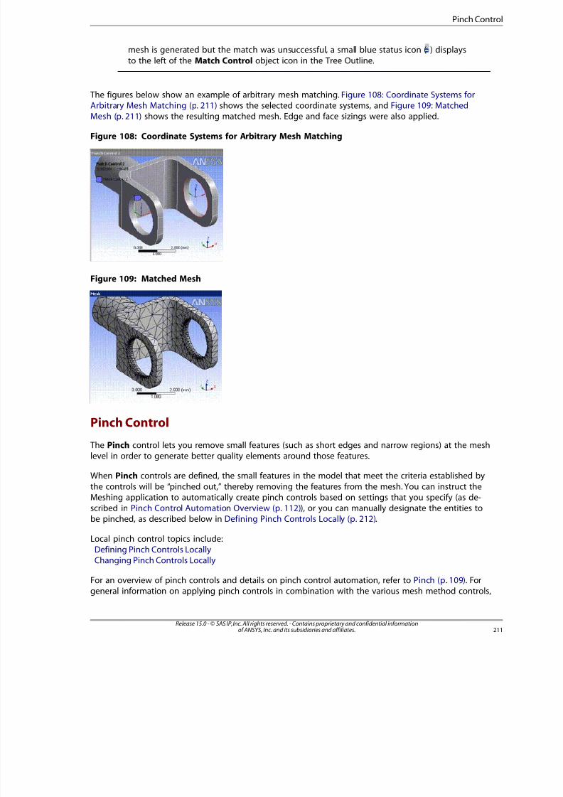
8/10/2019 ANSYS Meshing Users Guide
http://slidepdf.com/reader/full/ansys-meshing-users-guide 219/491
mesh is generated but the match was unsuccessful, a small blue status icon ( ) displays
to the left of the Match Control object icon in the Tree Outline.
The figures below show an example of arbitrary mesh matching. Figure 108: Coordinate Systems forArbitrary Mesh Matching (p. 211) shows the selected coordinate systems, and Figure 109: MatchedMesh (p. 211) shows the resulting matched mesh. Edge and face sizings were also applied.
Figure 108: Coordinate Systems for Arbitrary Mesh Matching
Figure 109: Matched Mesh
Pinch Control
The Pinch control lets you remove small features (such as short edges and narrow regions) at the meshlevel in order to generate better quality elements around those features.
When Pinch controls are defined, the small features in the model that meet the criteria established by
the controls will be “pinched out,” thereby removing the features from the mesh. You can instruct the
Meshing application to automatically create pinch controls based on settings that you specify (as de-scribed in Pinch Control Automation Overview (p. 112)), or you can manually designate the entities tobe pinched, as described below in Defining Pinch Controls Locally (p. 212).
Local pinch control topics include:Defining Pinch Controls LocallyChanging Pinch Controls Locally
For an overview of pinch controls and details on pinch control automation, refer to Pinch (p. 109). Forgeneral information on applying pinch controls in combination with the various mesh method controls,
21Release 15.0 - © SAS IP, Inc. All rights reserved. - Contains proprietary and confidential informationof ANSYS, Inc. and its subsidiaries and affiliates.
Pinch Contro

8/10/2019 ANSYS Meshing Users Guide
http://slidepdf.com/reader/full/ansys-meshing-users-guide 220/491
refer to "Meshing: Mesh Control Interaction Tables" (p. 345). For general information about pinch controlusage, see Usage Information for Pinch Controls (p. 117).
Defining Pinch Controls Locally
This section describes the steps for defining pinch controls locally.
To define pinch controls locally:
1. Click the Mesh folder in the Tree Outline. Right-click and select Insert > Pinch from the context menu.
Or
Click Mesh Control on the toolbar and choose Pinch from the menu.
A pinch control object is inserted into the Tree.
2. In the Geometry window, pick one or more faces, one or more edges, or one vertex that you want todefine as the master(s). (A master geometry is an entity that retains the profile of the original geometry.)Refer to Pinch (p. 109) for a table that summarizes the valid entities you can pick for each type of pinch
control.
3. Use either of these methods to apply your selection:
• Right-click in the Geometry window to display the context menu and select Set As Pinch Master.
• Click in the Master Geometry field in the Details View.
The pinch region is flagged in the Geometry window. The color of each selected entity changesto blue to identify it as master geometry. If you want to adjust your selections, you can re-pick geometry and then apply the new selections to overwrite the existing master geometry. If using
the context menu method to apply selections, you can also pick additional geometry and select
Add To Pinch Master to add the geometry to the existing master geometry. Also see ChangingPinch Controls Locally (p. 215).
4. In the Geometry window, pick one or more edges or vertices that you want to define as the slave(s).
(A slave geometry is an entity that changes in order to move towards the master geometry. Dependingon the tolerance, the pinch control will pinch out the entire slave entity or only a portion of the slaveentity into the master. Faces cannot be defined as slaves.)
5. Use either of these methods to apply your selection:
• Right-click in the Geometry window to display the context menu and select Set As Pinch Slave.
• Click in the Slave Geometry field in the Details View.
The color of each selected edge/vertex changes to red to identify it as slave geometry. If you wantto adjust your selections, you can re-pick geometry and then apply the new selections to overwritethe existing slave geometry. If using the context menu method to apply selections, you can alsopick additional geometry and select Add To Pinch Slave to add the geometry to the existing slave
geometry. Also see Changing Pinch Controls Locally (p. 215).
6. Change the value of the Suppressed control if desired.
Release 15.0 - © SAS IP, Inc. All rights reserved. - Contains proprietary and confidential informationof ANSYS, Inc. and its subsidiaries and affiliates.212
Local Mesh Controls

8/10/2019 ANSYS Meshing Users Guide
http://slidepdf.com/reader/full/ansys-meshing-users-guide 221/491
By default, the value of Suppressed is No. If you change the value to Yes, this pinch control hasno effect on the mesh (that is, the small features you picked for this pinch control are not removed
and will affect the mesh). In addition, an Active control with a read-only setting of No, Suppressedappears under the Suppressed control when Suppressed is set to Yes.
7. Change the value of the Tolerance control if desired.
By default, the value of Tolerance is based on the global pinch control tolerance. If you specify a
different value here, it overrides the global value.
8. Change the value of the Snap to Boundary control if desired.
By default, the value of Snap to Boundary is Yes. Snap to Boundary is applicable only for pinchcontrols in shell models for which a face has been defined as the master geometry and one ormore edges are defined as the slave(s). In such cases, when the value of Snap to Boundary is Yesand the distance from a slave edge to the closest mesh boundary of the master face is within the
specified snap to boundary tolerance, nodes from the slave edge are projected onto the boundaryof the master face. The joined edge will be on the master face along with other edges on themaster face that fall within the defined pinch control tolerance. Refer to the figures below to see
the effect of the Snap to Boundary setting.
Note
For edge-to-edge pinch controls in shell models, the snap tolerance is set equal to thepinch tolerance internally and cannot be modified.
9. Change the value of the Snap Type control if desired. Snap Type appears only when the value of Sna
to Boundary is Yes.
• If Snap Type is set to Manual Tolerance (the default), a Snap Tolerance field appears where you
may enter a numerical value greater than 0. By default, the Snap Tolerance is set equal to the pinchtolerance but it can be overridden here.
• If Snap Type is set to Element Size Factor, a Master Element Size Factor field appears where youmay enter a numerical value greater than 0. The value entered should be a factor of the local elemesize of the master topology.
10. Change the value of the PinchBehavior control if desired.
The default value of PinchBehavior, and whether it can be changed, is dependent on characteristicsof the model as shown in the table below. When set to Pre, pinches are processed before face
meshing, and when set to Post, pinches are processed in a separate step after all meshing iscomplete.
Note
• Toggling suppression of post pinch controls or changing their properties causes bodies
affected by those pinch controls to have an unmeshed state. However, when you sub-sequently select Generate Mesh, only the post pinch controls will be regenerated. Sincethese controls are a post mesh process, a remesh is not necessary and will not occur.
213Release 15.0 - © SAS IP, Inc. All rights reserved. - Contains proprietary and confidential informationof ANSYS, Inc. and its subsidiaries and affiliates.
Pinch Contro
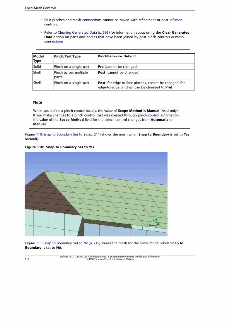
8/10/2019 ANSYS Meshing Users Guide
http://slidepdf.com/reader/full/ansys-meshing-users-guide 222/491
• Post pinches and mesh connections cannot be mixed with refinement or post inflationcontrols.
• Refer to Clearing Generated Data (p. 363) for information about using the Clear GeneratedData option on parts and bodies that have been joined by post pinch controls or meshconnections.
PinchBehavior DefaultPinch/Part TypeModelType
Pre (cannot be changed)Pinch on a single partSolid
Post (cannot be changed)Pinch across multiple
parts
Shell
Post (for edge-to-face pinches, cannot be changed; for
edge-to-edge pinches, can be changed to Pre)
Pinch on a single partShell
Note
When you define a pinch control locally, the value of Scope Method is Manual (read-only).
If you make changes to a pinch control that was created through pinch control automation,the value of the Scope Method field for that pinch control changes from Automatic toManual.
Figure 110: Snap to Boundary Set to Yes (p. 214) shows the mesh when Snap to Boundary is set to Yes
(default).
Figure 110: Snap to Boundary Set to Yes
Figure 111: Snap to Boundary Set to No (p. 215) shows the mesh for the same model when Snap to
Boundary is set to No.
Release 15.0 - © SAS IP, Inc. All rights reserved. - Contains proprietary and confidential informationof ANSYS, Inc. and its subsidiaries and affiliates.214
Local Mesh Controls
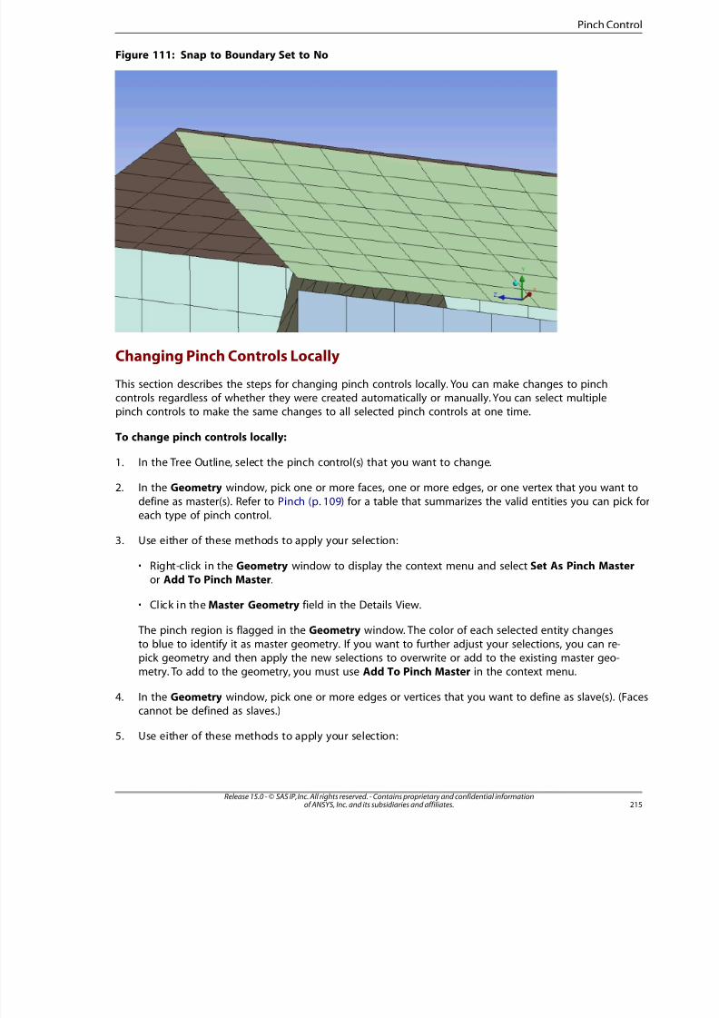
8/10/2019 ANSYS Meshing Users Guide
http://slidepdf.com/reader/full/ansys-meshing-users-guide 223/491
Figure 111: Snap to Boundary Set to No
Changing Pinch Controls Locally
This section describes the steps for changing pinch controls locally. You can make changes to pinchcontrols regardless of whether they were created automatically or manually. You can select multiplepinch controls to make the same changes to all selected pinch controls at one time.
To change pinch controls locally:
1. In the Tree Outline, select the pinch control(s) that you want to change.
2. In the Geometry window, pick one or more faces, one or more edges, or one vertex that you want to
define as master(s). Refer to Pinch (p. 109) for a table that summarizes the valid entities you can pick feach type of pinch control.
3. Use either of these methods to apply your selection:
• Right-click in the Geometry window to display the context menu and select Set As Pinch Masteror Add To Pinch Master.
• Click in the Master Geometry field in the Details View.
The pinch region is flagged in the Geometry window. The color of each selected entity changes
to blue to identify it as master geometry. If you want to further adjust your selections, you can re-pick geometry and then apply the new selections to overwrite or add to the existing master geo-metry. To add to the geometry, you must use Add To Pinch Master in the context menu.
4. In the Geometry window, pick one or more edges or vertices that you want to define as slave(s). (Facecannot be defined as slaves.)
5. Use either of these methods to apply your selection:
215Release 15.0 - © SAS IP, Inc. All rights reserved. - Contains proprietary and confidential informationof ANSYS, Inc. and its subsidiaries and affiliates.
Pinch Contro
8/10/2019 ANSYS Meshing Users Guide
http://slidepdf.com/reader/full/ansys-meshing-users-guide 224/491
Right-click in the Geometry window to display the context menu and select Set As Pinch Slave orAdd To Pinch Slave.
•
• Click in the Slave Geometry field in the Details View.
The color of each selected edge/vertex changes to red to identify it as slave geometry. If you wantto further adjust your selections, you can re-pick geometry and then apply the new selections to
overwrite or add to the existing slave geometry. To add to the geometry, you must use Add To
Pinch Slave in the context menu.
6. Change the value of the Suppressed control if desired.
By default, the value of Suppressed is No. If you change the value to Yes, this pinch control hasno effect on the mesh (that is, the small features you picked for this pinch control are not removedand will affect the mesh). In addition, an Active control with a read-only setting of No, Suppressedappears under the Suppressed control when Suppressed is set to Yes.
7. Change the value of the Tolerance control if desired.
By default, the value of Tolerance is based on the global pinch control tolerance. If you specify a
different value here, it overrides the global value.
8. Change the value of the Snap to Boundary control if desired.
By default, the value of Snap to Boundary is Yes. Snap to Boundary is applicable only for pinchcontrols in shell models for which a face has been defined as the master geometry and one or
more edges are defined as the slave(s). In such cases, when the value of Snap to Boundary is Yesand the distance from a slave edge to the closest mesh boundary of the master face is within thespecified snap to boundary tolerance, nodes from the slave edge are projected onto the boundaryof the master face. The joined edge will be on the master face along with other edges on the
master face that fall within the defined pinch control tolerance. Refer to Figure 110: Snap toBoundary Set to Yes (p. 214) and Figure 111: Snap to Boundary Set to No (p. 215) to see the effect
of the setting.
Note
For edge-to-edge pinch controls in shell models, the snap tolerance is set equal to thepinch tolerance internally and cannot be modified.
9. Change the value of the Snap Type control if desired. Snap Type appears only when the value of Snapto Boundary is Yes.
• If Snap Type is set to Manual Tolerance (the default), a Snap Tolerance field appears where youmay enter a numerical value greater than 0. By default, the Snap Tolerance is set equal to the pinchtolerance but it can be overridden here.
• If Snap Type is set to Element Size Factor, a Master Element Size Factor field appears where youmay enter a numerical value greater than 0. The value entered should be a factor of the local elementsize of the master topology.
10. Change the value of the PinchBehavior control if desired.
Release 15.0 - © SAS IP, Inc. All rights reserved. - Contains proprietary and confidential informationof ANSYS, Inc. and its subsidiaries and affiliates.216
Local Mesh Controls
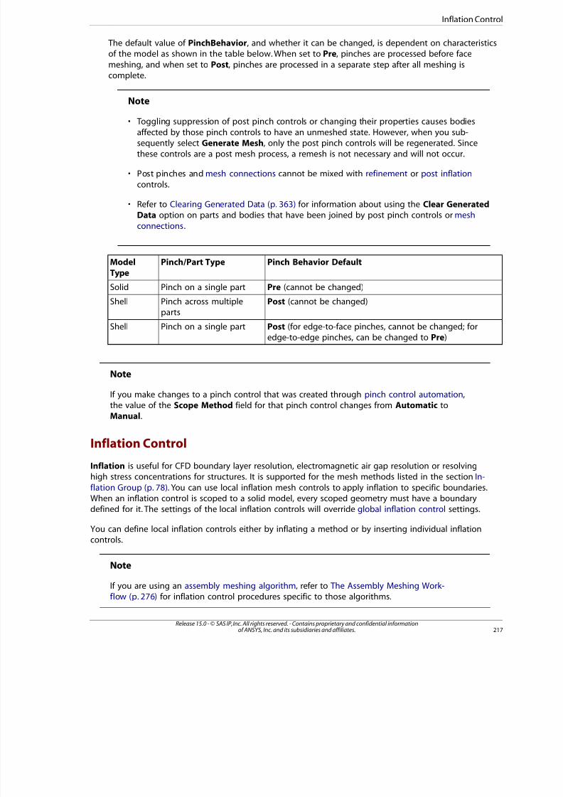
8/10/2019 ANSYS Meshing Users Guide
http://slidepdf.com/reader/full/ansys-meshing-users-guide 225/491
The default value of PinchBehavior, and whether it can be changed, is dependent on characteristicsof the model as shown in the table below. When set to Pre, pinches are processed before face
meshing, and when set to Post, pinches are processed in a separate step after all meshing iscomplete.
Note
• Toggling suppression of post pinch controls or changing their properties causes bodiesaffected by those pinch controls to have an unmeshed state. However, when you sub-sequently select Generate Mesh, only the post pinch controls will be regenerated. Sincethese controls are a post mesh process, a remesh is not necessary and will not occur.
• Post pinches and mesh connections cannot be mixed with refinement or post inflation
controls.
• Refer to Clearing Generated Data (p. 363) for information about using the Clear GeneratedData option on parts and bodies that have been joined by post pinch controls or mesh
connections.
Pinch Behavior DefaultPinch/Part TypeModel
Type
Pre (cannot be changed)Pinch on a single partSolid
Post (cannot be changed)Pinch across multipleparts
Shell
Post (for edge-to-face pinches, cannot be changed; foredge-to-edge pinches, can be changed to Pre)
Pinch on a single partShell
Note
If you make changes to a pinch control that was created through pinch control automation,the value of the Scope Method field for that pinch control changes from Automatic toManual.
Inflation Control
Inflation is useful for CFD boundary layer resolution, electromagnetic air gap resolution or resolvinghigh stress concentrations for structures. It is supported for the mesh methods listed in the section In-
flation Group (p. 78). You can use local inflation mesh controls to apply inflation to specific boundaries.
When an inflation control is scoped to a solid model, every scoped geometry must have a boundarydefined for it. The settings of the local inflation controls will override global inflation control settings.
You can define local inflation controls either by inflating a method or by inserting individual inflationcontrols.
Note
If you are using an assembly meshing algorithm, refer to The Assembly Meshing Work-flow (p. 276) for inflation control procedures specific to those algorithms.
217Release 15.0 - © SAS IP, Inc. All rights reserved. - Contains proprietary and confidential informationof ANSYS, Inc. and its subsidiaries and affiliates.
Inflation Contro

8/10/2019 ANSYS Meshing Users Guide
http://slidepdf.com/reader/full/ansys-meshing-users-guide 226/491
Inflating a Method
1. Insert a mesh method.
2. Associate (scope) the desired bodies with the method.
3. Right-click on the method and choose Inflate This Method from the menu.
Note
For example, if you click the right mouse button on a Tetrahedrons method control, oron a Sweep method control and specify the source, an Inflate This Method menu optionis available. Choosing this option inserts an inflation control on every body to which the
Tetrahedrons meshing method with the selected Algorithm is applied, or on every faceto which the Sweep method is applied. Similarly, an inflation control will be inserted intothe Tree Outline for each body/face. (Sweeping with inflation is the same as inflation with
tetrahedrons except that with sweeping you pick faces and edges instead of bodies andfaces.)
4. Highlight one of the inflation controls that was inserted into the Tree Outline.
5. Change the value of the Suppressed control if desired.
By default, the value of Suppressed is No. If you change the value to Yes, this inflation control hasno effect on the mesh. In addition, an Active control with a read-only setting of No, Suppressedappears under the Suppressed control when Suppressed is set to Yes.
6. Use either of these methods to specify the inflation boundaries:
• In the Details View, set Boundary Scoping Method to Geometry Selection, pick the entities in the
Geometry window, and click the Boundary field in the Details View to Apply.
• In the Details View, set Boundary Scoping Method to Named Selections, select a Named Selectionfrom the Boundary drop-down, and press Enter.
Note
– To select multiple Named Selections to be used as inflation boundaries, press and holdthe CTRL key while selecting the Named Selections from the Boundary drop-down, and
then press Enter.
– If none of the predefined Named Selections include the correct topology to be used as
an inflation boundary, no Named Selections will be available in the drop-down. For ex-ample, if you scoped a surface body with the method in step 2, a Named Selection con-taining an edge must exist. Otherwise, you cannot select anything from the drop-down.
7. Specify additional inflation options as desired. For details about options, refer to the notes below andto Inflation Group (p. 78).
8. Repeat steps 4 through 7 for each inflation control in the Tree Outline.
Release 15.0 - © SAS IP, Inc. All rights reserved. - Contains proprietary and confidential informationof ANSYS, Inc. and its subsidiaries and affiliates.218
Local Mesh Controls
8/10/2019 ANSYS Meshing Users Guide
http://slidepdf.com/reader/full/ansys-meshing-users-guide 227/491
Inserting Individual Inflation Controls
1. Optionally, select the desired bodies or faces in the Geometry window.
2. Use either of these methods to insert the inflation control:
• Click Mesh Control on the toolbar and choose Inflation from the menu.
• Right-click in the Geometry window and choose Insert > Inflation from the menu.
3. If you selected the bodies or faces in step 1, go directly to step 4. If not, use either of these methods to
scope inflation to the desired bodies or faces:
• In the Details View, set Scoping Method to Geometry Selection, pick the entities in the Geometrywindow, and click the Geometry field in the Details View to Apply.
• In the Details View, set Scoping Method to Named Selection, and select a Named Selection from th
Named Selection drop-down.
4. Change the value of the Suppressed control if desired.
By default, the value of Suppressed is No. If you change the value to Yes, this inflation control has
no effect on the mesh. In addition, an Active control with a read-only setting of No, Suppressedappears under the Suppressed control when Suppressed is set to Yes.
5. Use either of these methods to specify the inflation boundaries:
• In the Details View, set Boundary Scoping Method to Geometry Selection, pick the entities in theGeometry window, and click the Boundary field in the Details View to Apply.
• In the Details View, set Boundary Scoping Method to Named Selections, select a Named Selection
from the Boundary drop-down, and press Enter.
Note
– To select multiple Named Selections to be used as inflation boundaries, press and holdthe CTRL key while selecting the Named Selections from the Boundary drop-down, andthen press Enter.
– If none of the predefined Named Selections include the correct topology to be used asan inflation boundary, no Named Selections will be available in the drop-down. For ex-ample, if you selected a face in step 1, a Named Selection containing an edge must exist.
Otherwise, you cannot select anything from the drop-down.
6. Specify additional inflation options as desired. For details about options, refer to the notes below andto Inflation Group (p. 78).
Notes on Defining Local Inflation Controls (2D Only)
In most cases, the controls in the global Inflation group apply to both 3D and 2D inflation, and thevalues set globally will be populated to the local inflation controls. Changes that you make to the local
inflation settings will override the global settings. Exceptions and special considerations for defining2D local inflation are described here.
219Release 15.0 - © SAS IP, Inc. All rights reserved. - Contains proprietary and confidential informationof ANSYS, Inc. and its subsidiaries and affiliates.
Inflation Contro

8/10/2019 ANSYS Meshing Users Guide
http://slidepdf.com/reader/full/ansys-meshing-users-guide 228/491
• The ability to define 2D (face) inflation is not supported for assembly meshing algorithms.
• When defining 2D local inflation, the available options for the Inflation Option control are SmoothTransition (default), First Layer Thickness, and Total Thickness. If the Inflation Option control is setto First Aspect Ratio or Last Aspect Ratio globally, it will be set to Smooth Transition locally.
– When Inflation Option is Smooth Transition, you can set values for Transition Ratio (p. 85), Maximum
Layers (p. 85), and Growth Rate (p. 86).
– If you select First Layer Thickness, you can set values for First Layer Height (p. 86), Maximum Lay-ers (p. 85), and Growth Rate (p. 86). The value of Growth Rate is used to calculate the heights of the
successive layers, as follows:
Growth Rate = hn+1 / hn
where hn = height of layer n
– If you select Total Thickness, you can set values for Number of Layers (p. 86), Growth Rate (p. 86), andMaximum Thickness (p. 86). The first layer height is computed based on these three values. The heightsof the successive layers are computed using the same formula shown above under First Layer Thickness.
When 2D inflation is applied to a 3D model (i.e., to the face of a 3D body), the local value of MaximumLayers will be set equal to the global value by default. However, when it is applied to a 2D model (i.e, tothe face of a surface body), the local value of Maximum Layers will be set to 2.
• If you are using the Quadrilateral Dominant mesh method with inflation and the Advanced Size Function
is on, the mesh size of the last inflation layer will be used for the corresponding Quadrilateral Dominantboundary mesh size.
Notes on Defining Local Inflation Controls (3D and 2D)
• To make inflation boundary selection easier, select View > Annotations from the Main Menu to togglethe visibility of annotations in the Geometry window. For example, after scoping inflation to a body, the
body will be displayed using a blue solid annotation. Select View > Annotations to turn off the annotations;then select the desired faces as boundaries. For picking internal faces, the Hide Faces right mouse buttonoption may help you to see inside a body. For example, you can select external faces in the Geometrywindow and then use the Hide Faces option to hide the selected faces (making it easier to select the in-
ternal faces).
• Multiple Inflation controls can be scoped to the same body or face with different inflation options onthe faces/edges.
• If the mesh method is Automatic, the Patch Conforming tetrahedron method will be used for inflationon a body and the Sweep method will be used for inflation on a face.
• In the following scenarios, using inflation results in automatic suppression of the refinement control:
– When automatic inflation (either Program Controlled (p. 81) or All Faces in Chosen Named Selec-tion (p. 82)) is used with refinement in the same model
– When local inflation is used with refinement in the same body or in the same part
• For information on setting global inflation controls and descriptions of all of the individual inflation controls,refer to Inflation Group (p. 78). For steps to follow to assign inflation depending on the selected mesh
Release 15.0 - © SAS IP, Inc. All rights reserved. - Contains proprietary and confidential informationof ANSYS, Inc. and its subsidiaries and affiliates.220
Local Mesh Controls

8/10/2019 ANSYS Meshing Users Guide
http://slidepdf.com/reader/full/ansys-meshing-users-guide 229/491
method, refer to Inflation Controls (p. 316). For general information on applying inflation controls in combination with the various mesh method controls, refer to "Meshing: Mesh Control Interaction Tables" (p. 3
Sharp Angle Tool
Using the Sharp Angle Tool, you control the capture of features with sharp angles, such as the edge of
a knife or the region where a tire meets the road. It can also be used for improved feature capturingin general, even if the faces that you pick to define a control do not form a sharp angle. The SharpAngle Tool is available only when assembly meshing algorithms are being used and ensures that thedesired features are captured in the assembly mesh.
Using the Sharp Angle Tool
The steps for using the Sharp Angle Tool are presented here.
1. Highlight the Mesh object in the Tree Outline and then do one of the following:
• Click the right mouse button on the object and select Insert> Sharp Angle from the context menu.
• Select Mesh Control> Sharp Angle on the Mesh context toolbar.
• Click the right mouse button on the Geometry window and select Insert> Sharp Angle from thecontext menu.
These methods insert a sharp angle control beneath the Mesh object and activate the Face selection
filter.
2. Use either of these methods to scope the control to the desired faces:
• In the Details View, set Scoping Method to Geometry Selection, pick the faces in the Geometry
window, and click the Geometry field in the Details View to Apply.
• In the Details View, set Scoping Method to Named Selection, and select a Named Selection from thNamed Selection drop-down.
Note
If none of the predefined Named Selections include faces, no Named Selections willbe available in the drop-down.
3. Change the value of the Suppressed control if desired.
By default, the value of Suppressed is No. If you change the value to Yes, this control has no effecton the mesh (that is, the sharp angle features will not be captured). In addition, an Active controlwith a read-only setting of No, Suppressed appears under the Suppressed control when Suppressedis set to Yes.
Notes on the Sharp Angle Tool
• To suppress, unsuppress, or delete a sharp angle control, highlight it in the Tree Outline, click the right
mouse button, and select the appropriate option from the context menu. You cannot copy a sharp anglecontrol.
22Release 15.0 - © SAS IP, Inc. All rights reserved. - Contains proprietary and confidential informationof ANSYS, Inc. and its subsidiaries and affiliates.
Sharp Angle Too
8/10/2019 ANSYS Meshing Users Guide
http://slidepdf.com/reader/full/ansys-meshing-users-guide 230/491
• If any sharp angle controls are defined and you change from an assembly meshing algorithm to anothermesh method, the controls are suppressed automatically. In such cases, an Active control with a read-
only setting of No, Invalid Method will appear under the Suppressed control in the Details View, butthe value of the Suppressed control will still be set to No.
Gap Tool
The Gap Tool is applicable to Electromagnetic simulations where a refined mesh is required across anair gap in order to obtain accurate solutions. Typical applications are refined meshing in the air gapenclosure region of an actuator, or the air gap enclosure region between a rotor and a stator of a rotating
machine.
The tool identifies face/face pairs in a multibody part and creates gap sizing controls for meshing.Within a Gap Tool object, you can specify settings for sizing on the bodies adjacent to the gap and for
refinement of the mesh in the air gap.
Note
All Gap Tool controls and settings discussed in the following procedure are displayed only
when the model includes an enclosure from the DesignModeler application.
Using the Gap Tool
The steps for using the Gap Tool are presented here.
To use the Gap Tool:
1. Insert a Gap Tool object in the tree using one of the following procedures:
• Choose Mesh Control> Gap Tool on Mesh context toolbar.
• Click right mouse button on Mesh object (or any mesh control tool object)> Insert> Gap Tool.
2. Enter the width of the gap region between bodies (in your working units or as an existing CAD para-meter). This entry represents the range for multiple gaps, or equals a single gap distance that variesabout a certain tolerance. Your mesh density in the air gap is a direct function of the Gap Distance so
your gap size should be quite accurate.1 (p. 224) The applicable settings in the Details View are the fol-
lowing:
• Define By: Choose Range (default) if you will be entering numerical values, or CAD Parameters if you will be entering parameters to define the values.
• Minimum: The lower end of the range for multiple gaps, or the single gap distance.
• Maximum: (Optional) The upper end of the range for multiple gaps, or the single gap distance toler-ance.
After you set the gap distance, a crosshair appears adjacent to the cursor in the Geometry window. The crosshair is surrounded by a circle. The radius of the circle is a graphical indication of themaximum gap distance. The radius will change if you change this distance. The circle also appro-
priately adjusts when the model is zoomed in or out.
Release 15.0 - © SAS IP, Inc. All rights reserved. - Contains proprietary and confidential informationof ANSYS, Inc. and its subsidiaries and affiliates.222
Local Mesh Controls

8/10/2019 ANSYS Meshing Users Guide
http://slidepdf.com/reader/full/ansys-meshing-users-guide 231/491
3. Click the right mouse button on the Gap Tool object and choose Create Gap Sizes from the contextmenu. Workbench searches the model to find all occurrences of face pairs separated by the gap distan
you specified. All face pairs within an absolute distance from the minimum gap distance to the maximgap distance will have controls generated. Each occurrence of the gap face pairs is inserted as a GapSizing object under the Gap Tool object. By changing to Wireframe mode (Graphics toolbar) and
clicking through each Gap Sizing object, you can visually inspect the selected gap face pairs for usein mesh refinement.
Note
If you open a version 9.0 database file that includes Gap Sizing objects, Gap Tool ob- ject(s) are created automatically. These Gap Tool object(s) are reported in the tree with
a yellow lightning bolt status, meaning that the items are not in a valid state.
4. Right mouse click on Mesh object and choose Generate Mesh from the context menu.
5. Use the following controls to adjust the degree of sizing and mesh refinement, as needed, for the gap
face pairs. These controls appear in the Details View of the Gap Tool object.
• Gap Aspect Ratio: Slider control that adjusts the aspect ratio of elements in the gap between faces The ratio represents the length of an element edge parallel to the face pairs, to the width of theelement perpendicular to the face pairs. A lower ratio (for example, 1:1) will produce significantly
more elements than a higher ratio (for example, 4:1), but will generate better quality elements. Agood compromise is a value of 3:1 (default).
• Gap Density: Controls the number of elements spanning the width of the air gap between the face
pairs. The Coarse option (default) attempts to place at least two elements through the gap width,the Fine option attempts to place three to four elements through the gap width.
• Generate on Update: Controls whether the Gap Sizing objects are regenerated when the simulatio
is updated from the geometry. By default the Gap Sizing objects are regenerated at their defaultsettings. You may choose to not update a Gap Sizing object by selecting No. The No option willfreeze the Gap Sizing object's face pairs and settings. This option will only work properly if there arno topology changes for the face pairs during a geometry update. The Generate on Update featur
default setting is most applicable to rotating machines where the gap distance is constant but theGap Sizing object face pairs may change due to alignment. For linear devices (actuators), the Nooption may be preferred since the gap distance may change during a geometry update, but the facpairs will likely remain unchanged.
Note
For many applications, a typical Gap Aspect Ratio setting of 3:1 and Gap Density setto Coarse will produce good results. You may need to adjust the Curv/Proximity setting(refer to the description of Curvature and Proximity Refinement for related information)
in order to get a mesh. If this does not work, you may need to adjust the Gap AspectRatio or Gap Density settings or apply other size controls to the model.
223Release 15.0 - © SAS IP, Inc. All rights reserved. - Contains proprietary and confidential informationof ANSYS, Inc. and its subsidiaries and affiliates.
Gap Too

8/10/2019 ANSYS Meshing Users Guide
http://slidepdf.com/reader/full/ansys-meshing-users-guide 232/491
The Generate on Update field should be set to No to generate gap sizing controls withmultiple gap distances. Use multiple Gap Tool objects in this situation.
Note
Make sure that your maximum gap size is the actual gap size. A gap sizethat is too large will cause a meshing failure or incorrect size distribution.
1 - Algorithmic Notes
The size on the face pairs in regions that lie within the specified gap distance is determ-ined as follows:
Size = dG*GA
where:
dG = the maximum Gap Distance
GA = the Gap Aspect Ratio
Mesh refinement occurs across the gap on tetrahedron that lie within the gap.
If you have a very small gap, remember that the original size on the faces of the bodiesadjacent to the gap will be computed as described above. These elements may be difficultor impossible to refine if the gap is very small.
Release 15.0 - © SAS IP, Inc. All rights reserved. - Contains proprietary and confidential informationof ANSYS, Inc. and its subsidiaries and affiliates.224
Local Mesh Controls

8/10/2019 ANSYS Meshing Users Guide
http://slidepdf.com/reader/full/ansys-meshing-users-guide 233/491
Meshing: Options
You can control the behavior of functions in the Meshing application through the Options dialog box.For more information, refer to:
Accessing the Options Dialog Box
Meshing Options on the Options Dialog Box
Accessing the Options Dialog Box
To access the Meshing application options:
1. From the main menu, choose Tools> Options. An Options dialog box appears and the options are dis-played on the left.
2. Click on a specific option on the left (either Meshing or Export).
3. Change any of the option settings by clicking directly in the option field on the right. You will first seea visual indication for the kind of interaction required in the field (examples are drop-down menus, sec-ondary dialog boxes, direct text entries).
4. Click OK.
Note
• To cancel your changes and restore the default settings, click Reset on the Options dialog
box.
• Option settings within a particular language are independent of option settings in anotherlanguage. If you change any options from their default settings, then start a new Workbenchsession in a different language, the changes you made in the original language session are not
reflected in the new session. You are advised to make the same option changes in the newlanguage session.
Meshing Options on the Options Dialog Box
The options that appear in the right pane of the Options dialog box depend on which category is se-lected in the left pane:
• When Meshing is selected in the left pane, these subcategories appear:
– Meshing
– Virtual Topology
– Sizing
– Inflation
225Release 15.0 - © SAS IP, Inc. All rights reserved. - Contains proprietary and confidential informationof ANSYS, Inc. and its subsidiaries and affiliates.

8/10/2019 ANSYS Meshing Users Guide
http://slidepdf.com/reader/full/ansys-meshing-users-guide 234/491

8/10/2019 ANSYS Meshing Users Guide
http://slidepdf.com/reader/full/ansys-meshing-users-guide 235/491
the setting, when meshing completes and any bodies failed to mesh, the message “These bodies failedto be meshed” appears, and you can click the right mouse button to see them.
• Number of CPUs for Parallel Part Meshing : Sets the default number of processors to be used for paralpart meshing. You can change this value in the Advanced group under the Details view. Using the defafor specifying multiple processors will enhance meshing performance on geometries with multiple parts
For parallel part meshing, the default is set to Program Controlled or 0. This instructs the mesher to useall available CPU cores. The Default setting inherently limits 2 GB memory per CPU core. An explicit value
can be specified between 0 and 256, where 0 is the default. Parallel part meshing is currently only availaon 64–bit Windows. Refer to Parallel Part Meshing Best Practices (p. 228) for more details.
Virtual Topology
• Merge Edges Bounding Manually Created Faces: Sets the default value for the Merge Face Edges set
in the Details View of a Virtual Topology object. Choices are Yes and No. The default value is Yes.
Sizing
• Use Advanced Size Function: Sets the default value for the Use Advanced Size Function setting in the
Details View of a Mesh object. Choices are Off (the default), On: Proximity and Curvature, On: ProximiOn: Curvature, and On: Fixed.
Inflation
Inflation-related options that can be set on the Options dialog box include:
• Maximum Height over Base
• Gap Factor
• Growth Rate Type
• Maximum Angle (Degrees)
• Fillet Ratio
• Use Post Smoothing
• Smoothing Iterations
CGNS
• File Format: Sets the file format to be used for CGNS Export (p. 43) operations. There is no counterpartsetting in the Details View. Choices are:
– ADF (default) - Exports the mesh in ADF (Advanced Data Format).
– HDF5 - Exports the mesh in HDF5 (Hierarchical Data Format version 5).
• CGNS Version: Sets the CGNS library version to be used for CGNS Export (p. 43) operations. There is nocounterpart setting in the Details View. Choices are 3.1 (the default), 3.0, 2.5, 2.4, 2.3, 2.2, and 2.1.
227Release 15.0 - © SAS IP, Inc. All rights reserved. - Contains proprietary and confidential informationof ANSYS, Inc. and its subsidiaries and affiliates.
Meshing Options on the Options Dialog Box

8/10/2019 ANSYS Meshing Users Guide
http://slidepdf.com/reader/full/ansys-meshing-users-guide 236/491
ANSYS Fluent
• Format of Input File (*.msh): Sets the file format to be used for Fluent Mesh Export (p. 24) operations. There is no counterpart setting in the Details View. Choices are Binary (the default) and ASCII.
• Auto Zone Type Assignment: When set to On (the default), zone types are automatically assigned, asdescribed in Fluent Mesh Export (p. 24) . When set to Off , assigns all boundary zones as the default WALL,enabling you to assign your own zone type assignments for Fluent Mesh Export (p. 24) operations.
Parallel Part Meshing Best Practices
You can control three mechanisms in ANSYS Workbench that operate in a parallelized manner:
• Remote Solve Manager Design Point updates. Refer to Options Dialog Box.
• Parallel Part meshing (Windows 64–bit only): Tools> Options> Number of CPUs for Parallel PartMeshing
• Individual mesh methods (MultiZone Quad/Tri, Patch Independent Tetra, and MultiZone only):
Tools> Options> Number of CPUs for Meshing Methods
For the most efficient use of machine resources, it is important that the running processes do not over-saturate the processing cores or the available memory. You must allocate processing cores to each of
these mechanisms in a way that provides the most benefit for your workflow. When parallel partmeshing is invoked with the default number of of CPUs, it automatically uses the cores of all availableCPUs with the inherent limitation of 2 gigabytes per CPU core.
Best practices include:
• Know how many physical processing cores are available.
• If you are using Remote Solve Manager (RSM), meshing is done serially. This option cannot be over-
ridden.
• For non-RSM Design Point updates, meshing is done serially by default. You can override this optionby setting the option Number of CPUs for Parallel Part Meshing explicitly under Meshing>AdvancedOptions.
• If you are using more than one processor for individual meshing methods, be sure to set a balancebetween the two meshing options if you are using methods that support the Number of CPUs forMeshing Methods option (MultiZone Quad/Tri, Patch Independent Tetra, and MultiZone). Theyshould be set to an explicit value greater than 0.
For example, if you are using an 8 core system, setting Number of CPUs for Parallel Part
Meshing to 3 and Number of CPUs for Mesh Methods to 3 will provide a good balance. If themesh methods that you typically use support the Number of CPUs for Meshing Methods option,
setting the Number of CPUs for Parallel Part Meshing to 2 and the Number of CPUs forMeshing Methods to 4 or 5 may potentially provide more benefit.
• If you are using parallel part meshing only, you can set the Number of CPUs for Parallel PartMeshing to 0. In such cases, the software uses as many cores as possible.
• For Parallel Part meshing we recommend turning off hyper-threading as this may lead to degradationof parallel performance.
Release 15.0 - © SAS IP, Inc. All rights reserved. - Contains proprietary and confidential informationof ANSYS, Inc. and its subsidiaries and affiliates.228
Options

8/10/2019 ANSYS Meshing Users Guide
http://slidepdf.com/reader/full/ansys-meshing-users-guide 237/491
• Note that Parallel Part meshing does not support the following mesh controls:
– Assembly meshing
– Contact Sizing
– Fracture
– Manual Refinement
– Mesh Match via Symmetry
– Morph Service/Morphing
– Pinch
– Post Connection
– Post-Inflation
– Preview Surface Mesh/Preview Inflation
– Retry
– Refinement
229Release 15.0 - © SAS IP, Inc. All rights reserved. - Contains proprietary and confidential informationof ANSYS, Inc. and its subsidiaries and affiliates.
Meshing Options on the Options Dialog Box

8/10/2019 ANSYS Meshing Users Guide
http://slidepdf.com/reader/full/ansys-meshing-users-guide 238/491
Release 15.0 - © SAS IP, Inc. All rights reserved. - Contains proprietary and confidential informationof ANSYS, Inc. and its subsidiaries and affiliates.230
8/10/2019 ANSYS Meshing Users Guide
http://slidepdf.com/reader/full/ansys-meshing-users-guide 239/491
Meshing: Specialized Meshing
You can use the meshing features in ANSYS Workbench to perform various types of specialized meshing.For more information, refer to:
Mesh Sweeping
MultiZone MeshingAssembly MeshingSelective Meshing
Inflation ControlsMesh RefinementMixed Order MeshingAir Gap Meshing
Contact MeshingWinding Body MeshingWire Body MeshingPyramid Transitions
Match Meshing and the Symmetry FolderRigid Body Meshing Thin Solid Meshing
CAD Instance MeshingMeshing and Hard EntitiesBaffle MeshingFracture Meshing
Mesh Sweeping
This method of meshing complements the free mesher. If a body's topology is recognized as sweepable,
the body can be meshed very efficiently with hexahedral and wedge elements using this technique. The number of nodes and elements for a swept body is usually much smaller than ones meshed withthe free mesher. In addition, the time to create these elements is much smaller.
Workbench will automatically check to see if the body fulfills the topological requirements for sweeping.
It will then choose two faces that are topologically on the opposite sides of the body. These faces arecalled the source and target faces. Workbench will mesh the source face with quadrilateral and triangularelements and then copy that mesh onto the target face. It then generates either hexahedral or wedge
elements connecting the two faces and following the exterior topology of the body.
Note
• This information applies to general sweeping. For requirements and usage information specificto thin model sweeping, see Thin Model Sweeping (p. 238).
• For descriptions of the sweep option settings, see Sweep Method Control (p. 169).
23Release 15.0 - © SAS IP, Inc. All rights reserved. - Contains proprietary and confidential informationof ANSYS, Inc. and its subsidiaries and affiliates.
8/10/2019 ANSYS Meshing Users Guide
http://slidepdf.com/reader/full/ansys-meshing-users-guide 240/491
Requirements for General Sweeping
A body cannot be swept if any of these conditions exist:
• There is a completely contained internal void in the body.
• A source and target pair cannot be found. That is, the sweeper cannot find at least one path from a sourcesurface to a target surface connected by edges or closed surfaces.
• If a Sizing control is used on a body with hard edge sizing and the source and target faces contain harddivisions which are not the same for each respective edge.
When sweeping it is only necessary to apply hard divisions to one leg of the sweep path. If the pathhas multiple edges, you should apply your controls to that path.
If the sweep path is shared by another body and that path lies on the body's source or target face then
more hard divisions may be needed to constrain the sweeper.
When using Virtual Topology with sweeping, avoid creating virtual cells that result in a fully closedsurface. Fully closed surfaces cause difficulties for the swept mesher and may result in poor meshes.
When selecting adjacent faces for inclusion in a virtual cell, it is best to use Virtual Topology to mergesome (but not all) of the faces. A good approach is to use Virtual Topology for the smaller faces, butomit any larger faces from the virtual cell.
To preview any bodies that can be swept meshed, click Mesh on the Tree Outline and right-click the
mouse. Select Show> Sweepable Bodies from the context menu to display bodies that fulfill the re-quirements of a sweepable body. However, even if these requirements are met, the shape of the bodymay at times still result in poorly shaped elements. In these cases, the tetrahedron mesher is used to
mesh the body.
The Show Sweepable Bodies feature only displays bodies that can be swept where the source andtarget are not adjacent on an axis. It cannot automatically determine axis-sweepable bodies. However,
more enhanced sweeping capability, including axis-sweeping, is available by using the Sweep optionof the Method mesh control.
For help in diagnosing problems when using the Sweep method, refer to the description of the EdgeGraphics Options toolbar in the Mechanical help. This toolbar provides access to features that are in-
tended to improve your ability to distinguish edge and mesh connectivity.
Other Characteristics of General Sweeping
Other characteristics of sweeping include the following:
• The general sweeper ignores the Num Cells Across Gap setting, which is used to help define the proximity
size function.
• Hard entities are not supported for the general sweeper.
• If the sweep method is applied to a body and a Mapped Face Meshing control is defined for either thebody's source or target face, the sweep mesher will fail if a mapped mesh cannot be obtained for theface. See Notes on the Mapped Face Meshing Control (p. 202) for related information.
• The source and target faces do not have to be flat or parallel.
Release 15.0 - © SAS IP, Inc. All rights reserved. - Contains proprietary and confidential informationof ANSYS, Inc. and its subsidiaries and affiliates.232
Specialized Meshing
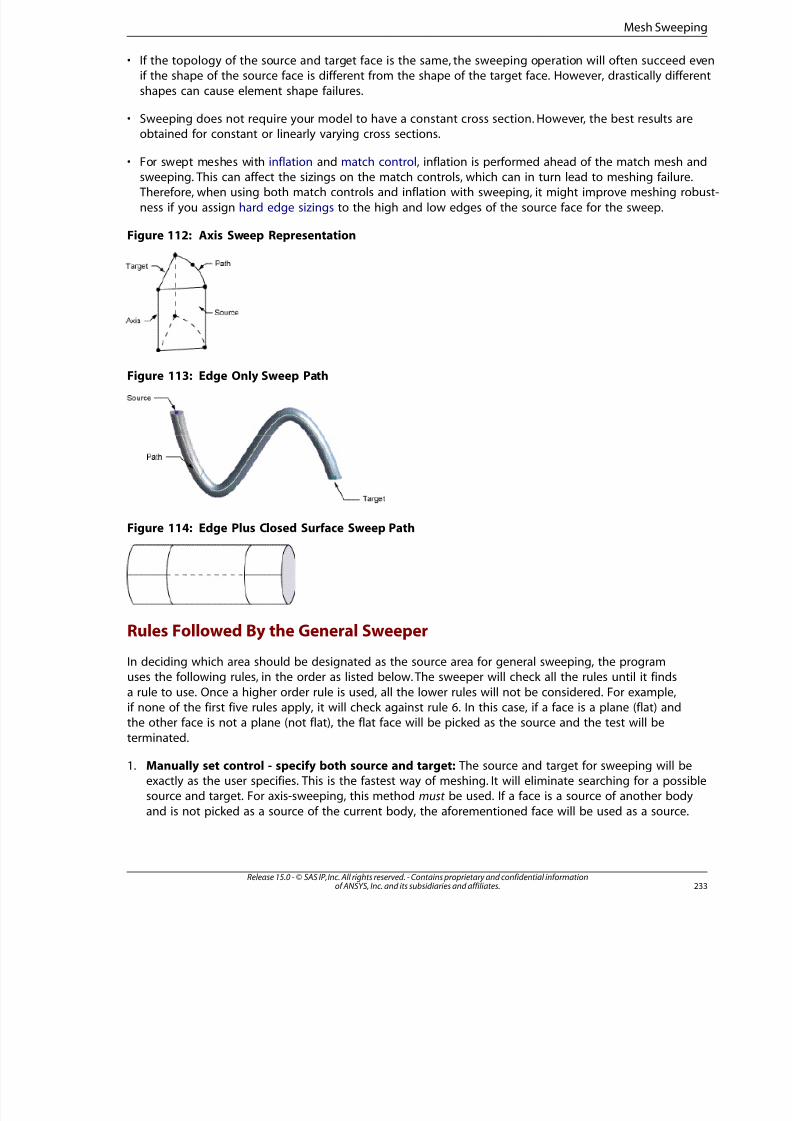
8/10/2019 ANSYS Meshing Users Guide
http://slidepdf.com/reader/full/ansys-meshing-users-guide 241/491
• If the topology of the source and target face is the same, the sweeping operation will often succeed eveif the shape of the source face is different from the shape of the target face. However, drastically differen
shapes can cause element shape failures.
• Sweeping does not require your model to have a constant cross section. However, the best results areobtained for constant or linearly varying cross sections.
• For swept meshes with inflation and match control, inflation is performed ahead of the match mesh and
sweeping. This can affect the sizings on the match controls, which can in turn lead to meshing failure. Therefore, when using both match controls and inflation with sweeping, it might improve meshing robu
ness if you assign hard edge sizings to the high and low edges of the source face for the sweep.
Figure 112: Axis Sweep Representation
Figure 113: Edge Only Sweep Path
Figure 114: Edge Plus Closed Surface Sweep Path
Rules Followed By the General Sweeper
In deciding which area should be designated as the source area for general sweeping, the programuses the following rules, in the order as listed below. The sweeper will check all the rules until it finds
a rule to use. Once a higher order rule is used, all the lower rules will not be considered. For example,
if none of the first five rules apply, it will check against rule 6. In this case, if a face is a plane (flat) andthe other face is not a plane (not flat), the flat face will be picked as the source and the test will be
terminated.
1. Manually set control - specify both source and target: The source and target for sweeping will beexactly as the user specifies. This is the fastest way of meshing. It will eliminate searching for a possiblesource and target. For axis-sweeping, this method must be used. If a face is a source of another body
and is not picked as a source of the current body, the aforementioned face will be used as a source.
233Release 15.0 - © SAS IP, Inc. All rights reserved. - Contains proprietary and confidential informationof ANSYS, Inc. and its subsidiaries and affiliates.
Mesh Sweeping
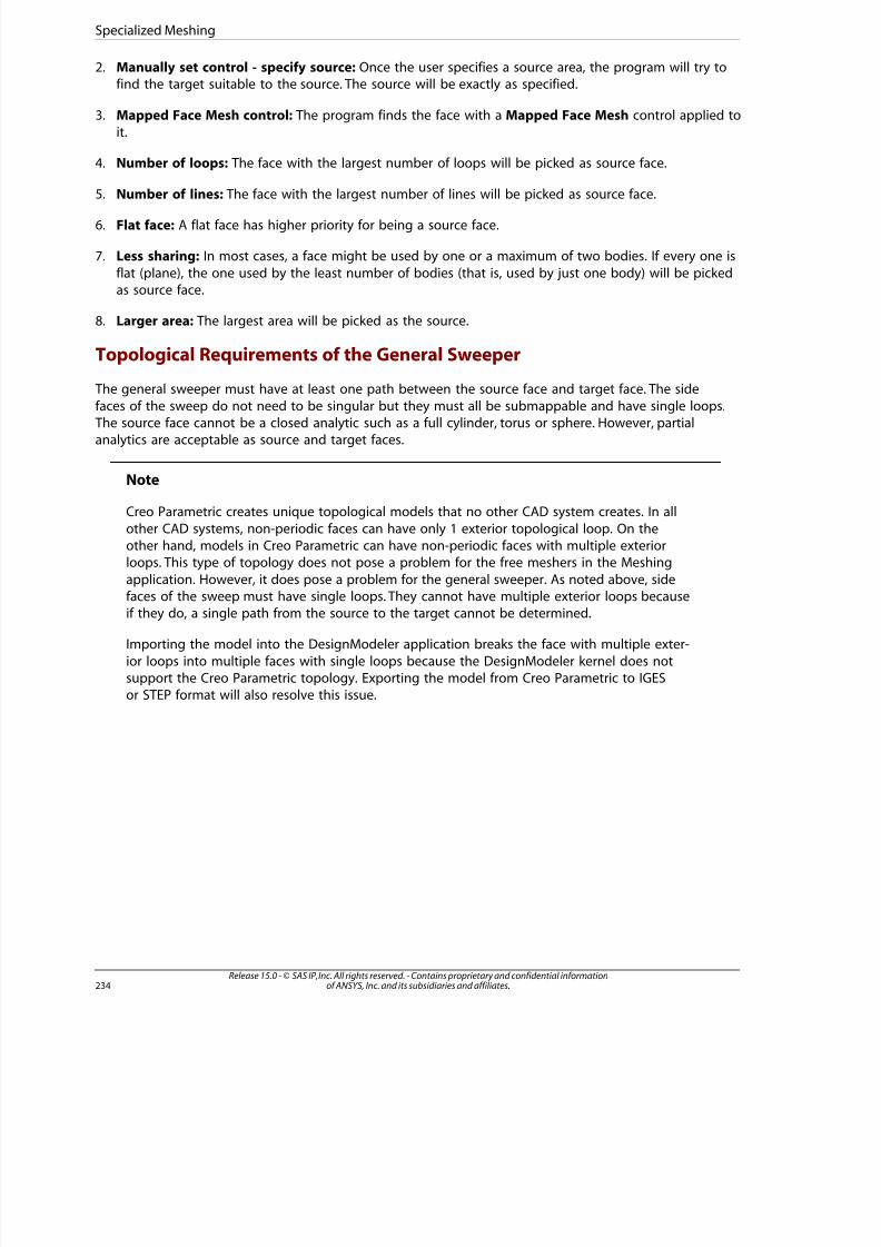
8/10/2019 ANSYS Meshing Users Guide
http://slidepdf.com/reader/full/ansys-meshing-users-guide 242/491
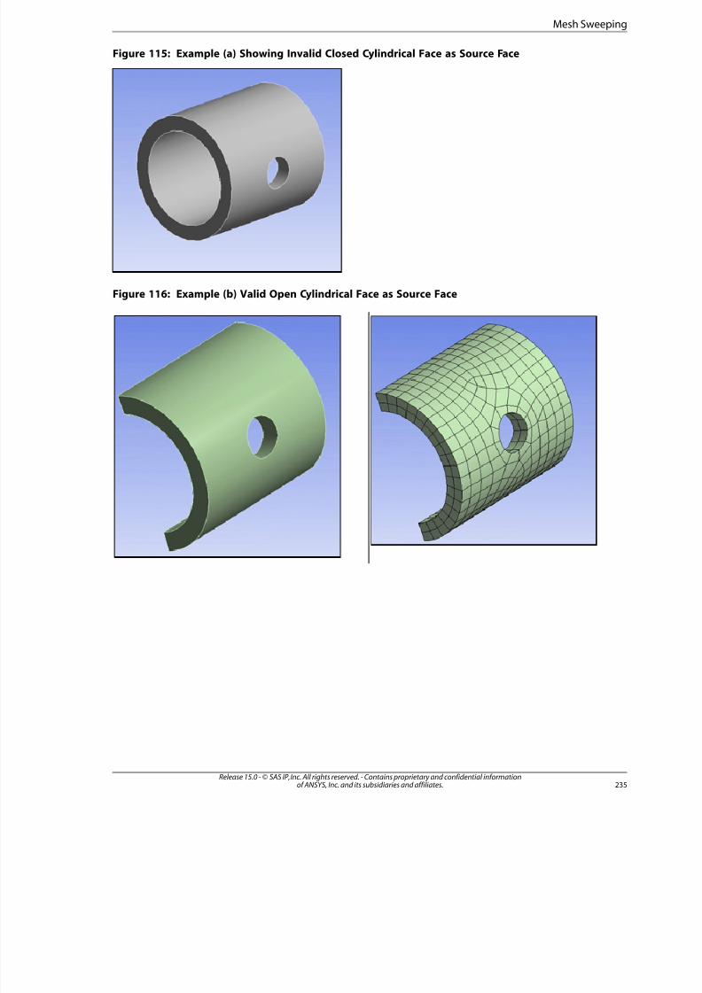
8/10/2019 ANSYS Meshing Users Guide
http://slidepdf.com/reader/full/ansys-meshing-users-guide 243/491
Figure 115: Example (a) Showing Invalid Closed Cylindrical Face as Source Face
Figure 116: Example (b) Valid Open Cylindrical Face as Source Face
235Release 15.0 - © SAS IP, Inc. All rights reserved. - Contains proprietary and confidential informationof ANSYS, Inc. and its subsidiaries and affiliates.
Mesh Sweeping
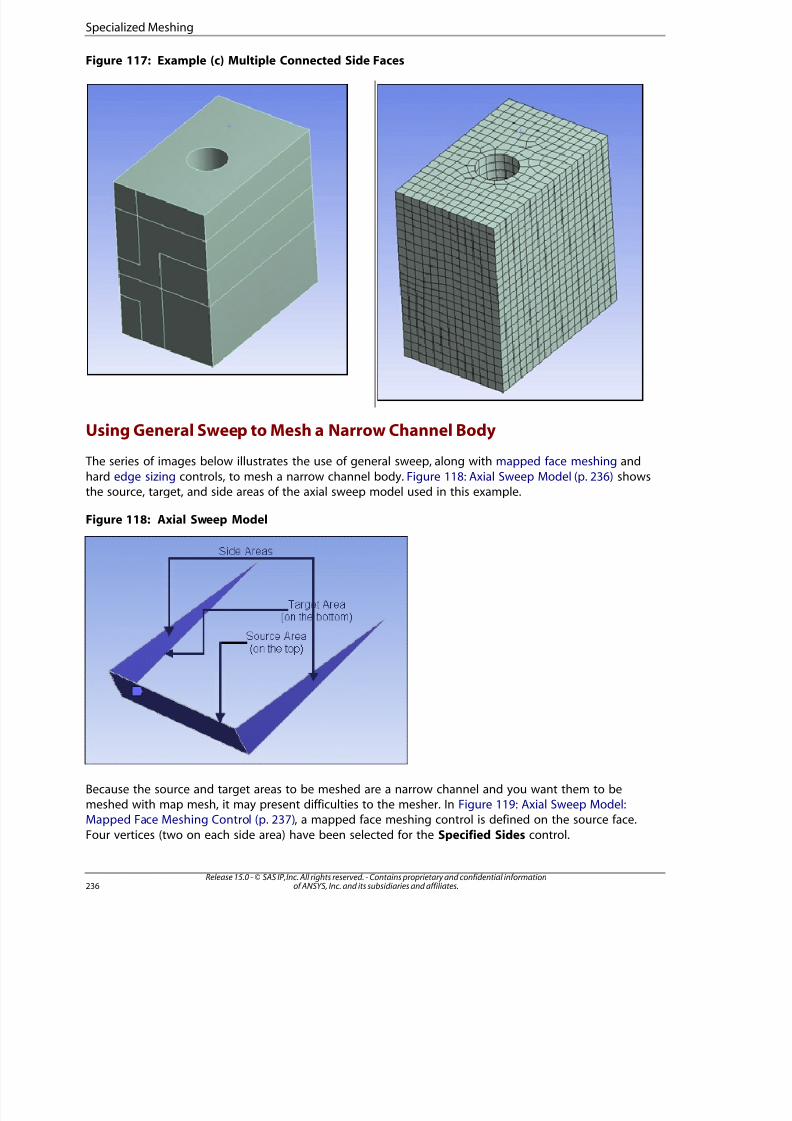
8/10/2019 ANSYS Meshing Users Guide
http://slidepdf.com/reader/full/ansys-meshing-users-guide 244/491
Figure 117: Example (c) Multiple Connected Side Faces
Using General Sweep to Mesh a Narrow Channel Body
The series of images below illustrates the use of general sweep, along with mapped face meshing and
hard edge sizing controls, to mesh a narrow channel body. Figure 118: Axial Sweep Model (p. 236) showsthe source, target, and side areas of the axial sweep model used in this example.
Figure 118: Axial Sweep Model
Because the source and target areas to be meshed are a narrow channel and you want them to bemeshed with map mesh, it may present difficulties to the mesher. In Figure 119: Axial Sweep Model:Mapped Face Meshing Control (p. 237), a mapped face meshing control is defined on the source face.
Four vertices (two on each side area) have been selected for the Specified Sides control.
Release 15.0 - © SAS IP, Inc. All rights reserved. - Contains proprietary and confidential informationof ANSYS, Inc. and its subsidiaries and affiliates.236
Specialized Meshing
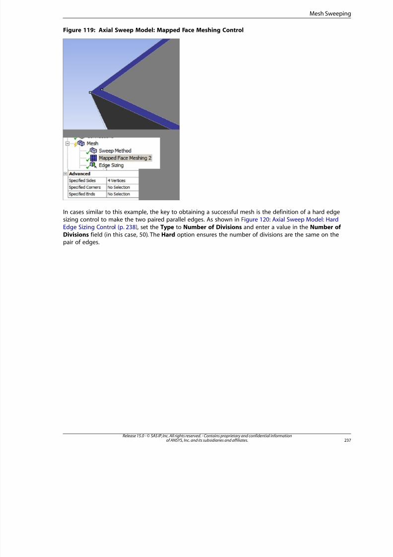
8/10/2019 ANSYS Meshing Users Guide
http://slidepdf.com/reader/full/ansys-meshing-users-guide 245/491
Figure 119: Axial Sweep Model: Mapped Face Meshing Control
In cases similar to this example, the key to obtaining a successful mesh is the definition of a hard edgesizing control to make the two paired parallel edges. As shown in Figure 120: Axial Sweep Model: Hard
Edge Sizing Control (p. 238), set the Type to Number of Divisions and enter a value in the Number of Divisions field (in this case, 50). The Hard option ensures the number of divisions are the same on thepair of edges.
237Release 15.0 - © SAS IP, Inc. All rights reserved. - Contains proprietary and confidential informationof ANSYS, Inc. and its subsidiaries and affiliates.
Mesh Sweeping
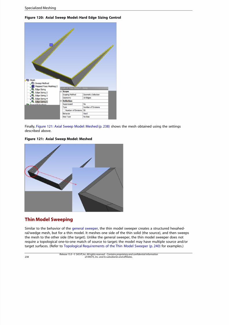
8/10/2019 ANSYS Meshing Users Guide
http://slidepdf.com/reader/full/ansys-meshing-users-guide 246/491
Figure 120: Axial Sweep Model: Hard Edge Sizing Control
Finally, Figure 121: Axial Sweep Model: Meshed (p. 238) shows the mesh obtained using the settingsdescribed above.
Figure 121: Axial Sweep Model: Meshed
Thin Model Sweeping
Similar to the behavior of the general sweeper, the thin model sweeper creates a structured hexahed-
ral/wedge mesh, but for a thin model. It meshes one side of the thin solid (the source), and then sweepsthe mesh to the other side (the target). Unlike the general sweeper, the thin model sweeper does notrequire a topological one-to-one match of source to target; the model may have multiple source and/ortarget surfaces. (Refer to Topological Requirements of the Thin Model Sweeper (p. 240) for examples.)
Release 15.0 - © SAS IP, Inc. All rights reserved. - Contains proprietary and confidential informationof ANSYS, Inc. and its subsidiaries and affiliates.238
Specialized Meshing
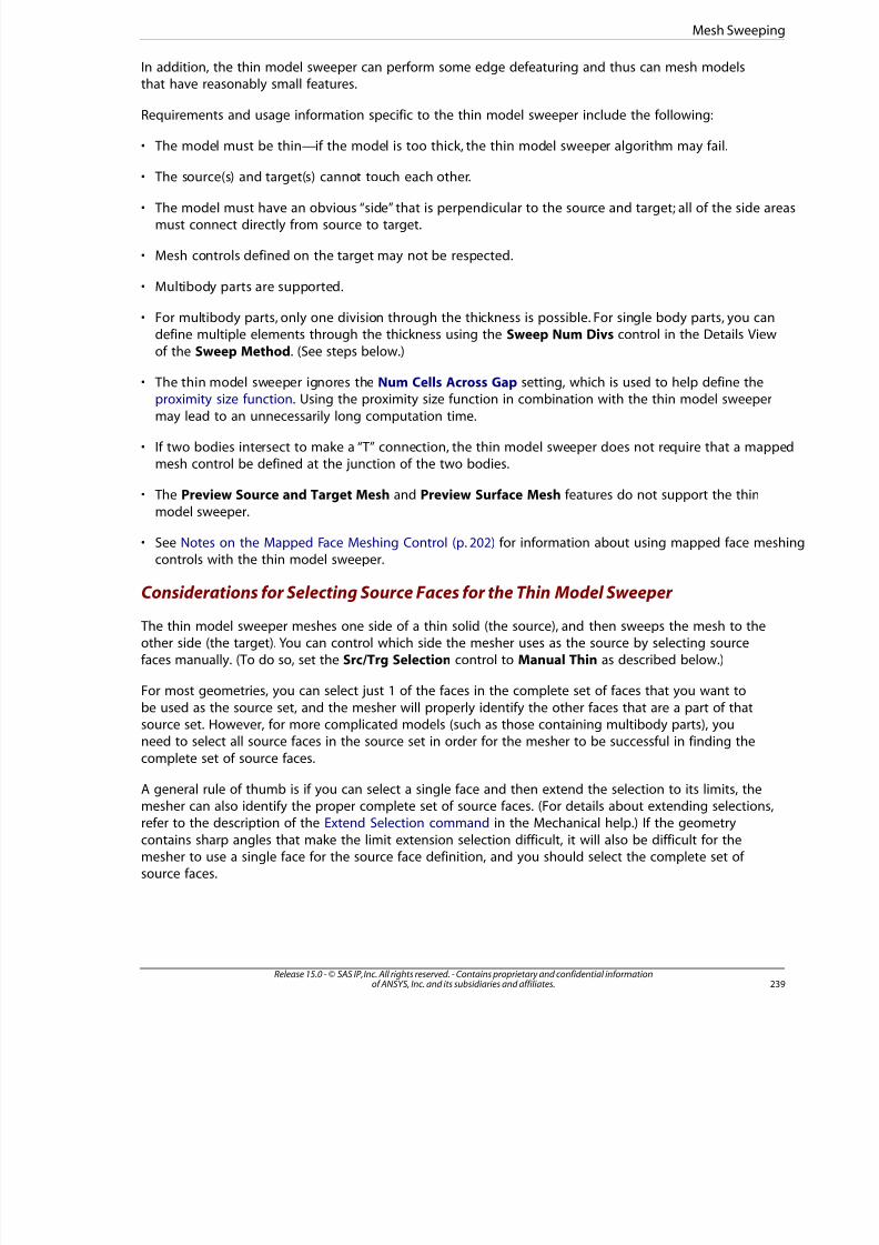
8/10/2019 ANSYS Meshing Users Guide
http://slidepdf.com/reader/full/ansys-meshing-users-guide 247/491
In addition, the thin model sweeper can perform some edge defeaturing and thus can mesh modelsthat have reasonably small features.
Requirements and usage information specific to the thin model sweeper include the following:
• The model must be thin—if the model is too thick, the thin model sweeper algorithm may fail.
• The source(s) and target(s) cannot touch each other.
• The model must have an obvious “side” that is perpendicular to the source and target; all of the side aremust connect directly from source to target.
• Mesh controls defined on the target may not be respected.
• Multibody parts are supported.
• For multibody parts, only one division through the thickness is possible. For single body parts, you candefine multiple elements through the thickness using the Sweep Num Divs control in the Details View
of the Sweep Method. (See steps below.)
• The thin model sweeper ignores the Num Cells Across Gap setting, which is used to help define theproximity size function. Using the proximity size function in combination with the thin model sweeper
may lead to an unnecessarily long computation time.
• If two bodies intersect to make a “T” connection, the thin model sweeper does not require that a mappemesh control be defined at the junction of the two bodies.
• The Preview Source and Target Mesh and Preview Surface Mesh features do not support the thin
model sweeper.
• See Notes on the Mapped Face Meshing Control (p. 202) for information about using mapped face meshcontrols with the thin model sweeper.
Considerations for Selecting Source Faces for the Thin Model Sweeper
The thin model sweeper meshes one side of a thin solid (the source), and then sweeps the mesh to theother side (the target). You can control which side the mesher uses as the source by selecting sourcefaces manually. (To do so, set the Src/Trg Selection control to Manual Thin as described below.)
For most geometries, you can select just 1 of the faces in the complete set of faces that you want to
be used as the source set, and the mesher will properly identify the other faces that are a part of thatsource set. However, for more complicated models (such as those containing multibody parts), youneed to select all source faces in the source set in order for the mesher to be successful in finding the
complete set of source faces.
A general rule of thumb is if you can select a single face and then extend the selection to its limits, themesher can also identify the proper complete set of source faces. (For details about extending selections,refer to the description of the Extend Selection command in the Mechanical help.) If the geometry
contains sharp angles that make the limit extension selection difficult, it will also be difficult for themesher to use a single face for the source face definition, and you should select the complete set of source faces.
239Release 15.0 - © SAS IP, Inc. All rights reserved. - Contains proprietary and confidential informationof ANSYS, Inc. and its subsidiaries and affiliates.
Mesh Sweeping
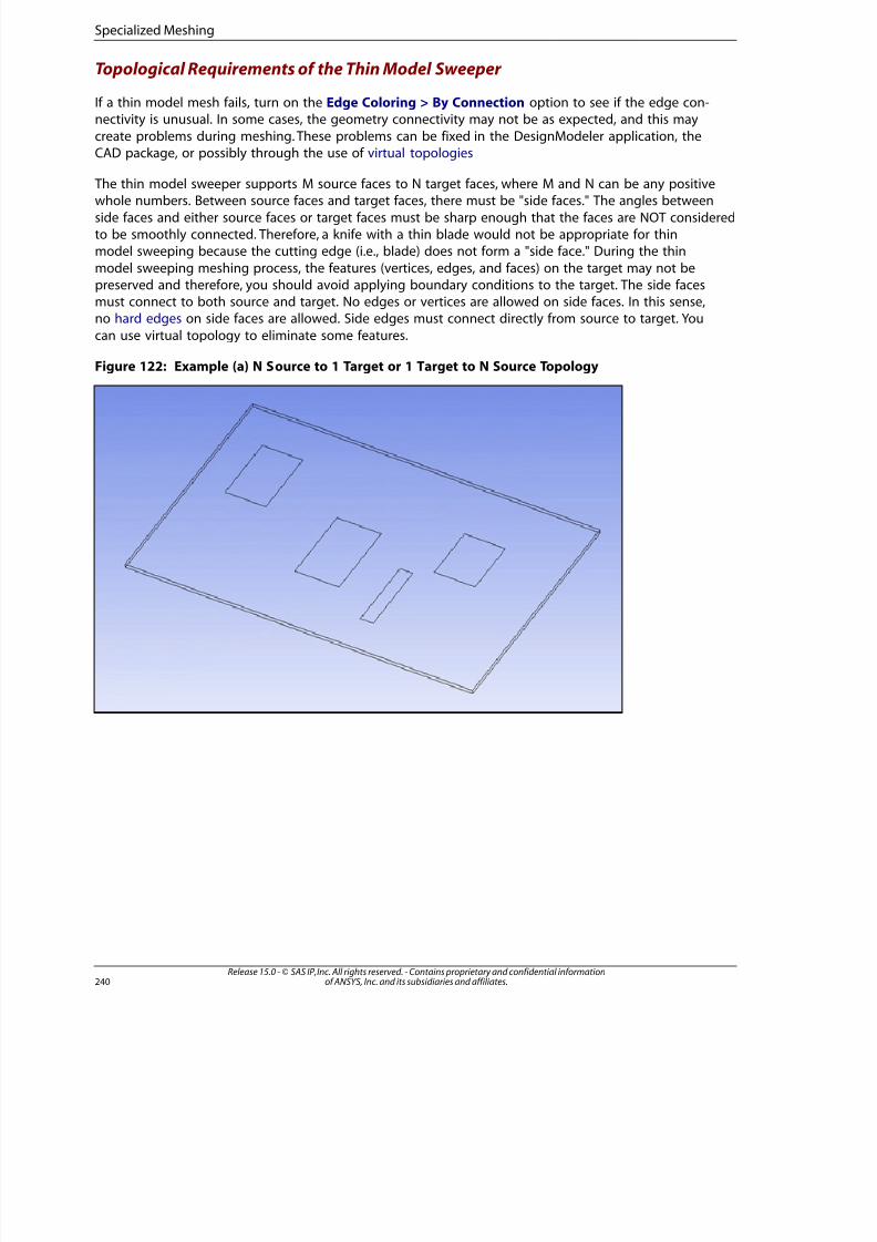
8/10/2019 ANSYS Meshing Users Guide
http://slidepdf.com/reader/full/ansys-meshing-users-guide 248/491
Topological Requirements of the Thin Model Sweeper
If a thin model mesh fails, turn on the Edge Coloring > By Connection option to see if the edge con-nectivity is unusual. In some cases, the geometry connectivity may not be as expected, and this may
create problems during meshing. These problems can be fixed in the DesignModeler application, theCAD package, or possibly through the use of virtual topologies
The thin model sweeper supports M source faces to N target faces, where M and N can be any positivewhole numbers. Between source faces and target faces, there must be "side faces." The angles between
side faces and either source faces or target faces must be sharp enough that the faces are NOT consideredto be smoothly connected. Therefore, a knife with a thin blade would not be appropriate for thinmodel sweeping because the cutting edge (i.e., blade) does not form a "side face." During the thin
model sweeping meshing process, the features (vertices, edges, and faces) on the target may not bepreserved and therefore, you should avoid applying boundary conditions to the target. The side facesmust connect to both source and target. No edges or vertices are allowed on side faces. In this sense,no hard edges on side faces are allowed. Side edges must connect directly from source to target. You
can use virtual topology to eliminate some features.
Figure 122: Example (a) N Source to 1 Target or 1 Target to N Source Topology
Release 15.0 - © SAS IP, Inc. All rights reserved. - Contains proprietary and confidential informationof ANSYS, Inc. and its subsidiaries and affiliates.240
Specialized Meshing
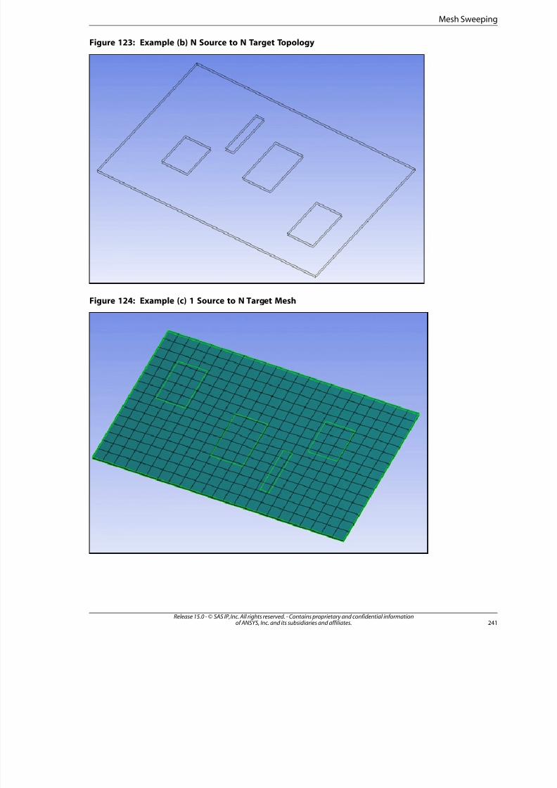
8/10/2019 ANSYS Meshing Users Guide
http://slidepdf.com/reader/full/ansys-meshing-users-guide 249/491
Figure 123: Example (b) N Source to N Target Topology
Figure 124: Example (c) 1 Source to N Target Mesh
24Release 15.0 - © SAS IP, Inc. All rights reserved. - Contains proprietary and confidential informationof ANSYS, Inc. and its subsidiaries and affiliates.
Mesh Sweeping
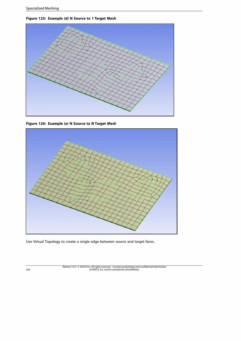
8/10/2019 ANSYS Meshing Users Guide
http://slidepdf.com/reader/full/ansys-meshing-users-guide 250/491
Figure 125: Example (d) N Source to 1 Target Mesh
Figure 126: Example (e) N Source to N Target Mesh
Use Virtual Topology to create a single edge between source and target faces.
Release 15.0 - © SAS IP, Inc. All rights reserved. - Contains proprietary and confidential informationof ANSYS, Inc. and its subsidiaries and affiliates.242
Specialized Meshing
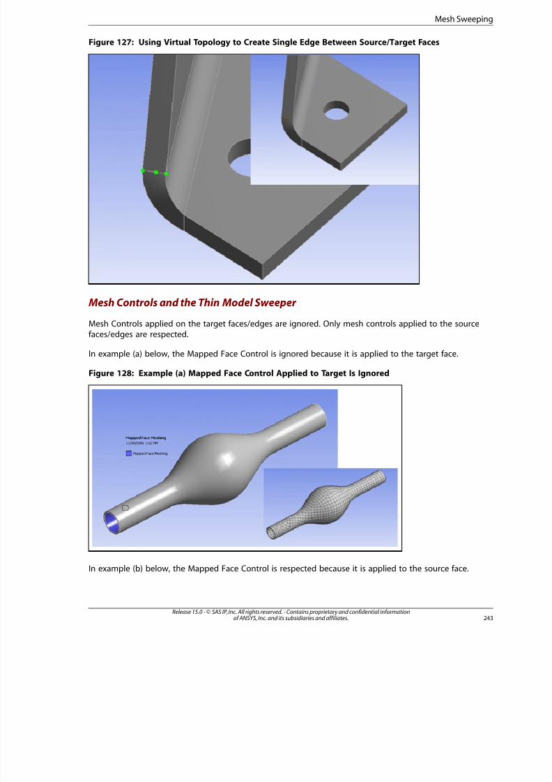
8/10/2019 ANSYS Meshing Users Guide
http://slidepdf.com/reader/full/ansys-meshing-users-guide 251/491
Figure 127: Using Virtual Topology to Create Single Edge Between Source/Target Faces
Mesh Controls and the Thin Model Sweeper
Mesh Controls applied on the target faces/edges are ignored. Only mesh controls applied to the sourcefaces/edges are respected.
In example (a) below, the Mapped Face Control is ignored because it is applied to the target face.
Figure 128: Example (a) Mapped Face Control Applied to Target Is Ignored
In example (b) below, the Mapped Face Control is respected because it is applied to the source face.
243Release 15.0 - © SAS IP, Inc. All rights reserved. - Contains proprietary and confidential informationof ANSYS, Inc. and its subsidiaries and affiliates.
Mesh Sweeping
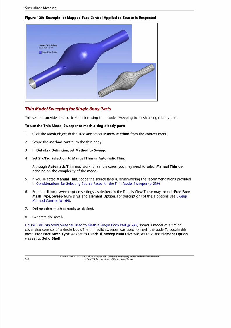
8/10/2019 ANSYS Meshing Users Guide
http://slidepdf.com/reader/full/ansys-meshing-users-guide 252/491
Figure 129: Example (b) Mapped Face Control Applied to Source Is Respected
Thin Model Sweeping for Single Body Parts
This section provides the basic steps for using thin model sweeping to mesh a single body part.
To use the Thin Model Sweeper to mesh a single body part:
1. Click the Mesh object in the Tree and select Insert> Method from the context menu.
2. Scope the Method control to the thin body.
3. In Details> Definition, set Method to Sweep.
4. Set Src/Trg Selection to Manual Thin or Automatic Thin.
Although Automatic Thin may work for simple cases, you may need to select Manual Thin de-pending on the complexity of the model.
5. If you selected Manual Thin, scope the source face(s), remembering the recommendations providedin Considerations for Selecting Source Faces for the Thin Model Sweeper (p. 239).
6. Enter additional sweep option settings, as desired, in the Details View. These may include Free Face
Mesh Type, Sweep Num Divs, and Element Option. For descriptions of these options, see SweepMethod Control (p. 169).
7. Define other mesh controls, as desired.
8. Generate the mesh.
Figure 130: Thin Solid Sweeper Used to Mesh a Single Body Part (p. 245) shows a model of a timingcover that consists of a single body. The thin solid sweeper was used to mesh the body. To obtain thismesh, Free Face Mesh Type was set to Quad/Tri, Sweep Num Divs was set to 2, and Element Option
was set to Solid Shell.
Release 15.0 - © SAS IP, Inc. All rights reserved. - Contains proprietary and confidential informationof ANSYS, Inc. and its subsidiaries and affiliates.244
Specialized Meshing
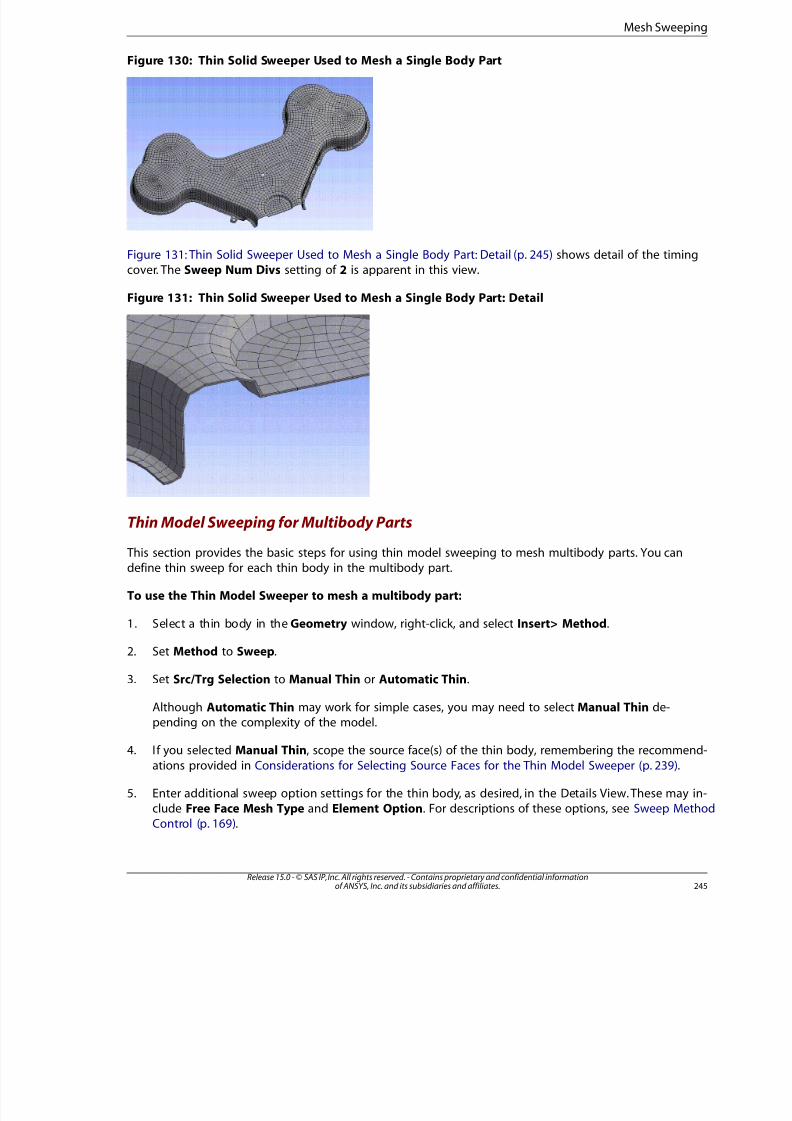
8/10/2019 ANSYS Meshing Users Guide
http://slidepdf.com/reader/full/ansys-meshing-users-guide 253/491
Figure 130: Thin Solid Sweeper Used to Mesh a Single Body Part
Figure 131: Thin Solid Sweeper Used to Mesh a Single Body Part: Detail (p. 245) shows detail of the timingcover. The Sweep Num Divs setting of 2 is apparent in this view.
Figure 131: Thin Solid Sweeper Used to Mesh a Single Body Part: Detail
Thin Model Sweeping for Multibody Parts This section provides the basic steps for using thin model sweeping to mesh multibody parts. You candefine thin sweep for each thin body in the multibody part.
To use the Thin Model Sweeper to mesh a multibody part:
1. Select a thin body in the Geometry window, right-click, and select Insert> Method.
2. Set Method to Sweep.
3. Set Src/Trg Selection to Manual Thin or Automatic Thin.
Although Automatic Thin may work for simple cases, you may need to select Manual Thin de-pending on the complexity of the model.
4. If you selected Manual Thin, scope the source face(s) of the thin body, remembering the recommend-
ations provided in Considerations for Selecting Source Faces for the Thin Model Sweeper (p. 239).
5. Enter additional sweep option settings for the thin body, as desired, in the Details View. These may in-clude Free Face Mesh Type and Element Option. For descriptions of these options, see Sweep MethoControl (p. 169).
245Release 15.0 - © SAS IP, Inc. All rights reserved. - Contains proprietary and confidential informationof ANSYS, Inc. and its subsidiaries and affiliates.
Mesh Sweeping
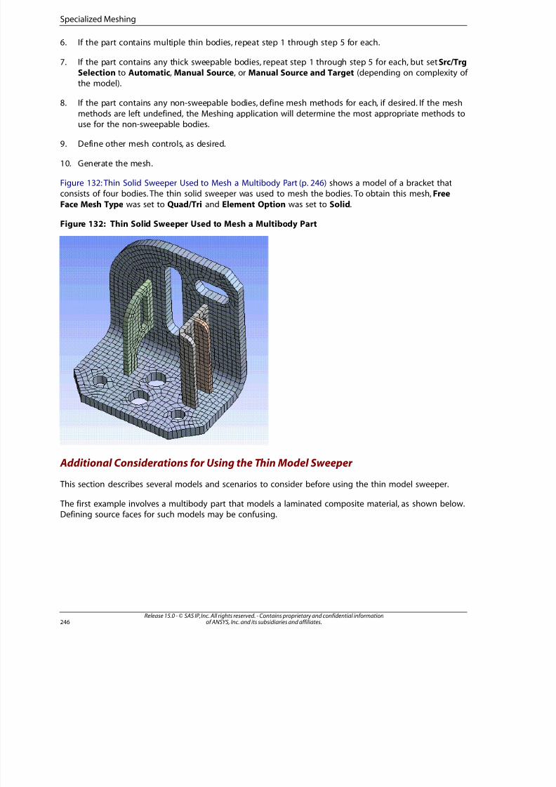
8/10/2019 ANSYS Meshing Users Guide
http://slidepdf.com/reader/full/ansys-meshing-users-guide 254/491
6. If the part contains multiple thin bodies, repeat step 1 through step 5 for each.
7. If the part contains any thick sweepable bodies, repeat step 1 through step 5 for each, but set Src/TrgSelection to Automatic, Manual Source, or Manual Source and Target (depending on complexity of the model).
8. If the part contains any non-sweepable bodies, define mesh methods for each, if desired. If the mesh
methods are left undefined, the Meshing application will determine the most appropriate methods to
use for the non-sweepable bodies.
9. Define other mesh controls, as desired.
10. Generate the mesh.
Figure 132: Thin Solid Sweeper Used to Mesh a Multibody Part (p. 246) shows a model of a bracket thatconsists of four bodies. The thin solid sweeper was used to mesh the bodies. To obtain this mesh, Free
Face Mesh Type was set to Quad/Tri and Element Option was set to Solid.
Figure 132: Thin Solid Sweeper Used to Mesh a Multibody Part
Additional Considerations for Using the Thin Model Sweeper
This section describes several models and scenarios to consider before using the thin model sweeper.
The first example involves a multibody part that models a laminated composite material, as shown below.Defining source faces for such models may be confusing.
Release 15.0 - © SAS IP, Inc. All rights reserved. - Contains proprietary and confidential informationof ANSYS, Inc. and its subsidiaries and affiliates.246
Specialized Meshing
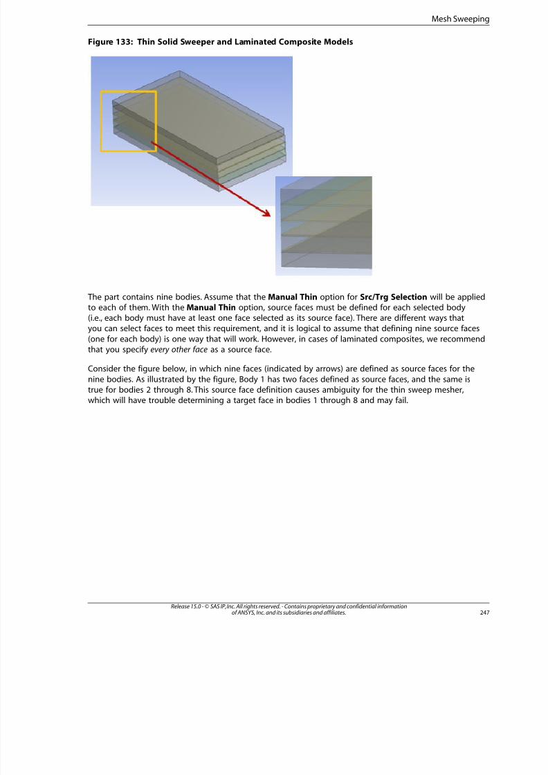
8/10/2019 ANSYS Meshing Users Guide
http://slidepdf.com/reader/full/ansys-meshing-users-guide 255/491
Figure 133: Thin Solid Sweeper and Laminated Composite Models
The part contains nine bodies. Assume that the Manual Thin option for Src/Trg Selection will be appliedto each of them. With the Manual Thin option, source faces must be defined for each selected body(i.e., each body must have at least one face selected as its source face). There are different ways thatyou can select faces to meet this requirement, and it is logical to assume that defining nine source faces
(one for each body) is one way that will work. However, in cases of laminated composites, we recommendthat you specify every other face as a source face.
Consider the figure below, in which nine faces (indicated by arrows) are defined as source faces for the
nine bodies. As illustrated by the figure, Body 1 has two faces defined as source faces, and the same istrue for bodies 2 through 8. This source face definition causes ambiguity for the thin sweep mesher,which will have trouble determining a target face in bodies 1 through 8 and may fail.
247Release 15.0 - © SAS IP, Inc. All rights reserved. - Contains proprietary and confidential informationof ANSYS, Inc. and its subsidiaries and affiliates.
Mesh Sweeping
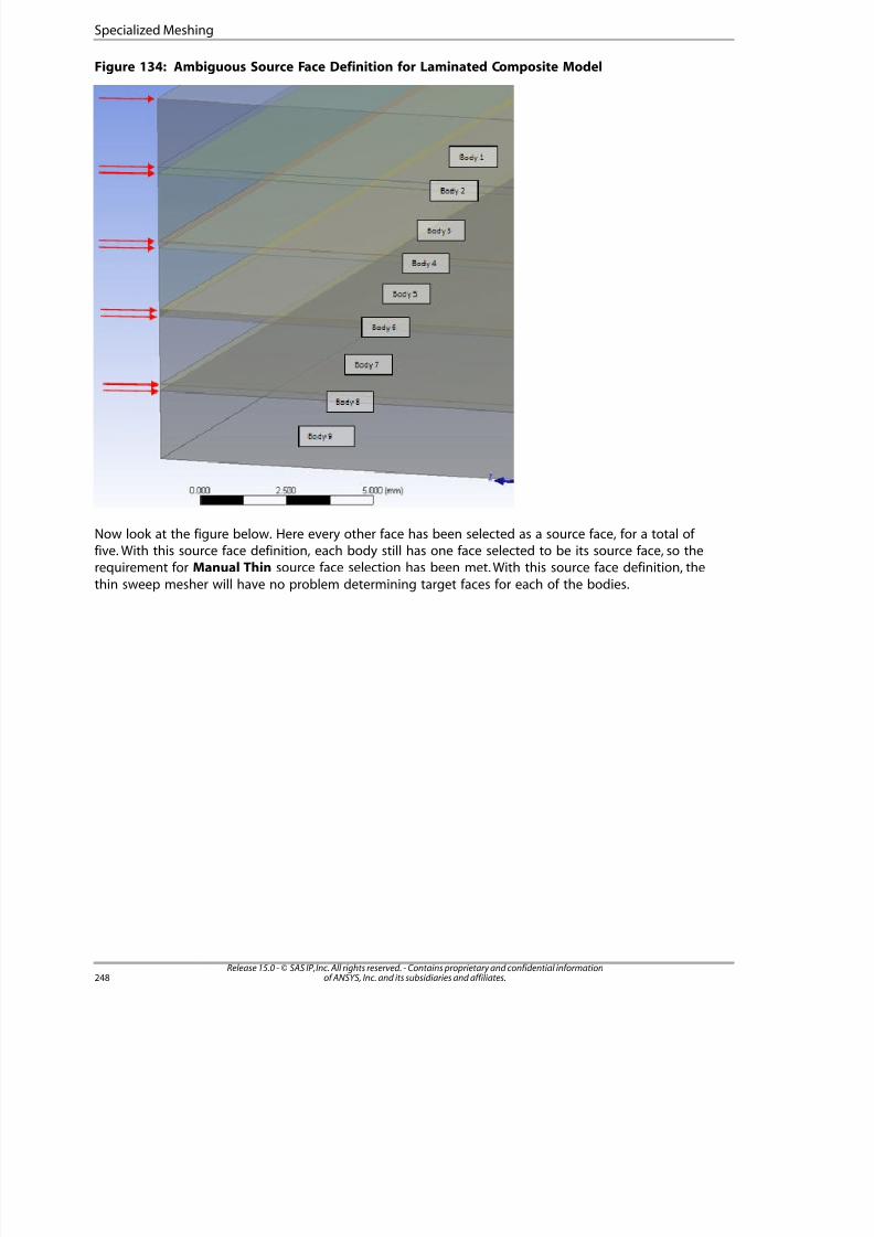
8/10/2019 ANSYS Meshing Users Guide
http://slidepdf.com/reader/full/ansys-meshing-users-guide 256/491
Figure 134: Ambiguous Source Face Definition for Laminated Composite Model
Now look at the figure below. Here every other face has been selected as a source face, for a total of five. With this source face definition, each body still has one face selected to be its source face, so therequirement for Manual Thin source face selection has been met. With this source face definition, the
thin sweep mesher will have no problem determining target faces for each of the bodies.
Release 15.0 - © SAS IP, Inc. All rights reserved. - Contains proprietary and confidential informationof ANSYS, Inc. and its subsidiaries and affiliates.248
Specialized Meshing
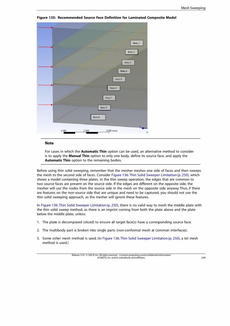
8/10/2019 ANSYS Meshing Users Guide
http://slidepdf.com/reader/full/ansys-meshing-users-guide 257/491
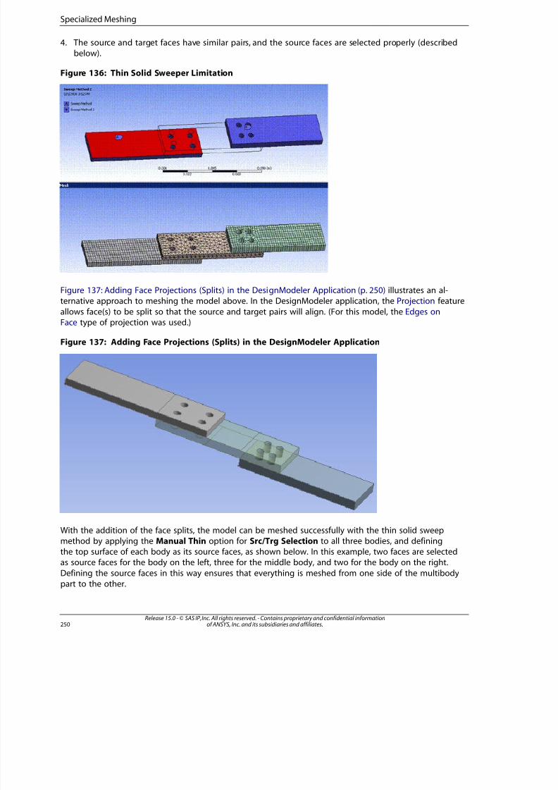
8/10/2019 ANSYS Meshing Users Guide
http://slidepdf.com/reader/full/ansys-meshing-users-guide 258/491
4. The source and target faces have similar pairs, and the source faces are selected properly (describedbelow).
Figure 136: Thin Solid Sweeper Limitation
Figure 137: Adding Face Projections (Splits) in the DesignModeler Application (p. 250) illustrates an al-ternative approach to meshing the model above. In the DesignModeler application, the Projection feature
allows face(s) to be split so that the source and target pairs will align. (For this model, the Edges onFace type of projection was used.)
Figure 137: Adding Face Projections (Splits) in the DesignModeler Application
With the addition of the face splits, the model can be meshed successfully with the thin solid sweepmethod by applying the Manual Thin option for Src/Trg Selection to all three bodies, and definingthe top surface of each body as its source faces, as shown below. In this example, two faces are selectedas source faces for the body on the left, three for the middle body, and two for the body on the right.
Defining the source faces in this way ensures that everything is meshed from one side of the multibodypart to the other.
Release 15.0 - © SAS IP, Inc. All rights reserved. - Contains proprietary and confidential informationof ANSYS, Inc. and its subsidiaries and affiliates.250
Specialized Meshing
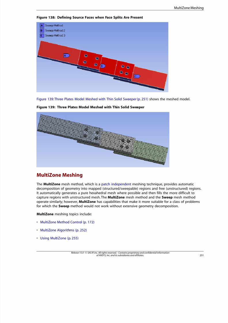
8/10/2019 ANSYS Meshing Users Guide
http://slidepdf.com/reader/full/ansys-meshing-users-guide 259/491
Figure 138: Defining Source Faces when Face Splits Are Present
Figure 139: Three Plates Model Meshed with Thin Solid Sweeper (p. 251) shows the meshed model.
Figure 139: Three Plates Model Meshed with Thin Solid Sweeper
MultiZone Meshing
The MultiZone mesh method, which is a patch independent meshing technique, provides automatic
decomposition of geometry into mapped (structured/sweepable) regions and free (unstructured) regions.It automatically generates a pure hexahedral mesh where possible and then fills the more difficult tocapture regions with unstructured mesh. The MultiZone mesh method and the Sweep mesh method
operate similarly; however, MultiZone has capabilities that make it more suitable for a class of problemsfor which the Sweep method would not work without extensive geometry decomposition.
MultiZone meshing topics include:
• MultiZone Method Control (p. 172)
• MultiZone Algorithms (p. 252)
• Using MultiZone (p. 255)
25Release 15.0 - © SAS IP, Inc. All rights reserved. - Contains proprietary and confidential informationof ANSYS, Inc. and its subsidiaries and affiliates.
MultiZone Meshing
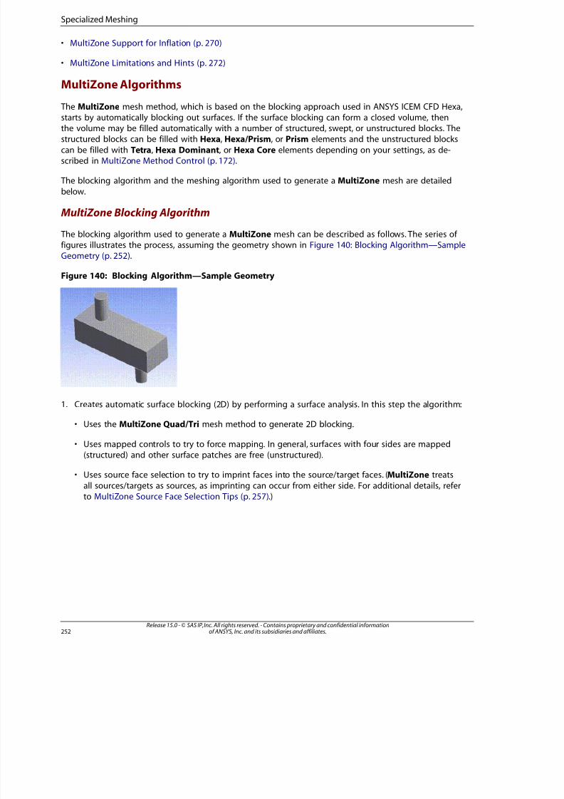
8/10/2019 ANSYS Meshing Users Guide
http://slidepdf.com/reader/full/ansys-meshing-users-guide 260/491
• MultiZone Support for Inflation (p. 270)
• MultiZone Limitations and Hints (p. 272)
MultiZone Algorithms
The MultiZone mesh method, which is based on the blocking approach used in ANSYS ICEM CFD Hexa,starts by automatically blocking out surfaces. If the surface blocking can form a closed volume, then
the volume may be filled automatically with a number of structured, swept, or unstructured blocks. Thestructured blocks can be filled with Hexa, Hexa/Prism, or Prism elements and the unstructured blocks
can be filled with Tetra, Hexa Dominant, or Hexa Core elements depending on your settings, as de-scribed in MultiZone Method Control (p. 172).
The blocking algorithm and the meshing algorithm used to generate a MultiZone mesh are detailed
below.
MultiZone Blocking Algorithm
The blocking algorithm used to generate a MultiZone mesh can be described as follows. The series of figures illustrates the process, assuming the geometry shown in Figure 140: Blocking Algorithm—SampleGeometry (p. 252).
Figure 140: Blocking Algorithm—Sample Geometry
1. Creates automatic surface blocking (2D) by performing a surface analysis. In this step the algorithm:
• Uses the MultiZone Quad/Tri mesh method to generate 2D blocking.
• Uses mapped controls to try to force mapping. In general, surfaces with four sides are mapped(structured) and other surface patches are free (unstructured).
• Uses source face selection to try to imprint faces into the source/target faces. (MultiZone treats
all sources/targets as sources, as imprinting can occur from either side. For additional details, referto MultiZone Source Face Selection Tips (p. 257).)
Release 15.0 - © SAS IP, Inc. All rights reserved. - Contains proprietary and confidential informationof ANSYS, Inc. and its subsidiaries and affiliates.252
Specialized Meshing
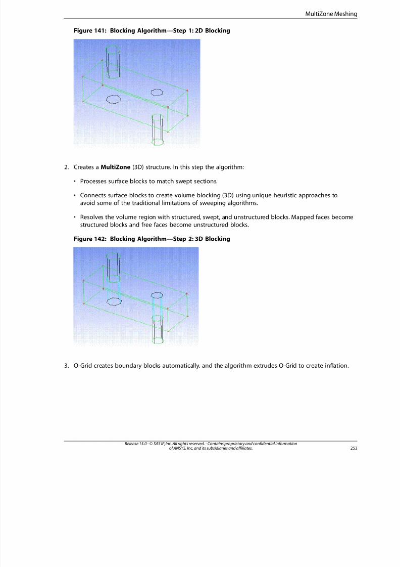
8/10/2019 ANSYS Meshing Users Guide
http://slidepdf.com/reader/full/ansys-meshing-users-guide 261/491
Figure 141: Blocking Algorithm—Step 1: 2D Blocking
2. Creates a MultiZone (3D) structure. In this step the algorithm:
• Processes surface blocks to match swept sections.
• Connects surface blocks to create volume blocking (3D) using unique heuristic approaches toavoid some of the traditional limitations of sweeping algorithms.
• Resolves the volume region with structured, swept, and unstructured blocks. Mapped faces becomestructured blocks and free faces become unstructured blocks.
Figure 142: Blocking Algorithm—Step 2: 3D Blocking
3. O-Grid creates boundary blocks automatically, and the algorithm extrudes O-Grid to create inflation.
253Release 15.0 - © SAS IP, Inc. All rights reserved. - Contains proprietary and confidential informationof ANSYS, Inc. and its subsidiaries and affiliates.
MultiZone Meshing

8/10/2019 ANSYS Meshing Users Guide
http://slidepdf.com/reader/full/ansys-meshing-users-guide 262/491
Figure 143: Blocking Algorithm—Step 3: Inflation
Note
Inflation can be performed on a combination of side and/or source faces.
MultiZone Meshing Algorithm
The meshing algorithm used to generate a MultiZone mesh can be described as follows:
• Assigns intervals by transferring sizing from the topology to blocking.
• Meshes structured faces (those that can be mapped meshed) using transfinite interpolation and un-structured (free) faces with all quadrilateral or a combination of quadrilateral/triangle elements.
• Interpolates, sweeps, and fills the volume mesh for the structured, swept, and unstructured blocks
respectively. The structured blocks can be filled with Hexa, Hexa/Prism, or Prism elements and theunstructured blocks can be filled with Tetra, Hexa Dominant, or Hexa Core elements dependingon your settings, as described in MultiZone Method Control (p. 172).
MultiZone for Sweepable Bodies
You can use the Show Sweepable Bodies setting to identify bodies that are meshed using the MultiZonemethod. Although MultiZone can mesh other, more complex bodies, it does not attempt this unlessyou manually insert MultiZone mesh method controls.
When you use Mesh Sweeping with MultiZone, MultiZone mesh method behaves in a patch conforming
way. That is, topology checks are skipped and you can scope boundary conditions, etc, after meshing
and the meshing will not go out of date.
If the swept mesh fails (it cannot create a valid mesh or any protected topology cannot be associated
correctly), the failing swept mesh bodies are changed into free swept mesh bodies, and the meshertries to create an unstructured tetra mesh.
Release 15.0 - © SAS IP, Inc. All rights reserved. - Contains proprietary and confidential informationof ANSYS, Inc. and its subsidiaries and affiliates.254
Specialized Meshing
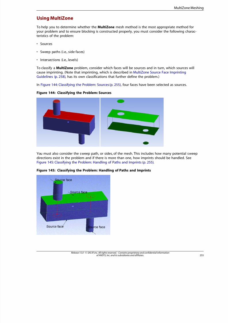
8/10/2019 ANSYS Meshing Users Guide
http://slidepdf.com/reader/full/ansys-meshing-users-guide 263/491
Using MultiZone
To help you to determine whether the MultiZone mesh method is the most appropriate method foryour problem and to ensure blocking is constructed properly, you must consider the following charac-teristics of the problem:
• Sources
• Sweep paths (i.e., side faces)
• Intersections (i.e., levels)
To classify a MultiZone problem, consider which faces will be sources and in turn, which sources willcause imprinting. (Note that imprinting, which is described in MultiZone Source Face ImprintingGuidelines (p. 258), has its own classifications that further define the problem.)
In Figure 144: Classifying the Problem: Sources (p. 255), four faces have been selected as sources.
Figure 144: Classifying the Problem: Sources
You must also consider the sweep path, or sides, of the mesh. This includes how many potential sweepdirections exist in the problem and if there is more than one, how imprints should be handled. See
Figure 145: Classifying the Problem: Handling of Paths and Imprints (p. 255).
Figure 145: Classifying the Problem: Handling of Paths and Imprints
255Release 15.0 - © SAS IP, Inc. All rights reserved. - Contains proprietary and confidential informationof ANSYS, Inc. and its subsidiaries and affiliates.
MultiZone Meshing
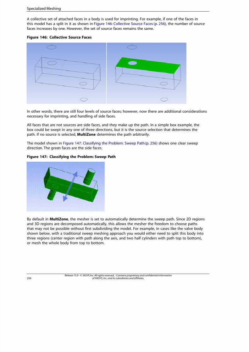
8/10/2019 ANSYS Meshing Users Guide
http://slidepdf.com/reader/full/ansys-meshing-users-guide 264/491
A collective set of attached faces in a body is used for imprinting. For example, if one of the faces inthis model has a split in it as shown in Figure 146: Collective Source Faces (p. 256), the number of source
faces increases by one. However, the set of source faces remains the same.
Figure 146: Collective Source Faces
In other words, there are still four levels of source faces; however, now there are additional considerationsnecessary for imprinting, and handling of side faces.
All faces that are not sources are side faces, and they make up the path. In a simple box example, thebox could be swept in any one of three directions, but it is the source selection that determines thepath. If no source is selected, MultiZone determines the path arbitrarily.
The model shown in Figure 147: Classifying the Problem: Sweep Path (p. 256) shows one clear sweepdirection. The green faces are the side faces.
Figure 147: Classifying the Problem: Sweep Path
By default in MultiZone, the mesher is set to automatically determine the sweep path. Since 2D regionsand 3D regions are decomposed automatically, this allows the mesher the freedom to choose pathsthat may not be possible without first subdividing the model. For example, in cases like the valve body
shown below, with a traditional sweep meshing approach you would either need to split this body intothree regions (center region with path along the axis, and two half cylinders with path top to bottom),or mesh the whole body from top to bottom.
Release 15.0 - © SAS IP, Inc. All rights reserved. - Contains proprietary and confidential informationof ANSYS, Inc. and its subsidiaries and affiliates.256
Specialized Meshing
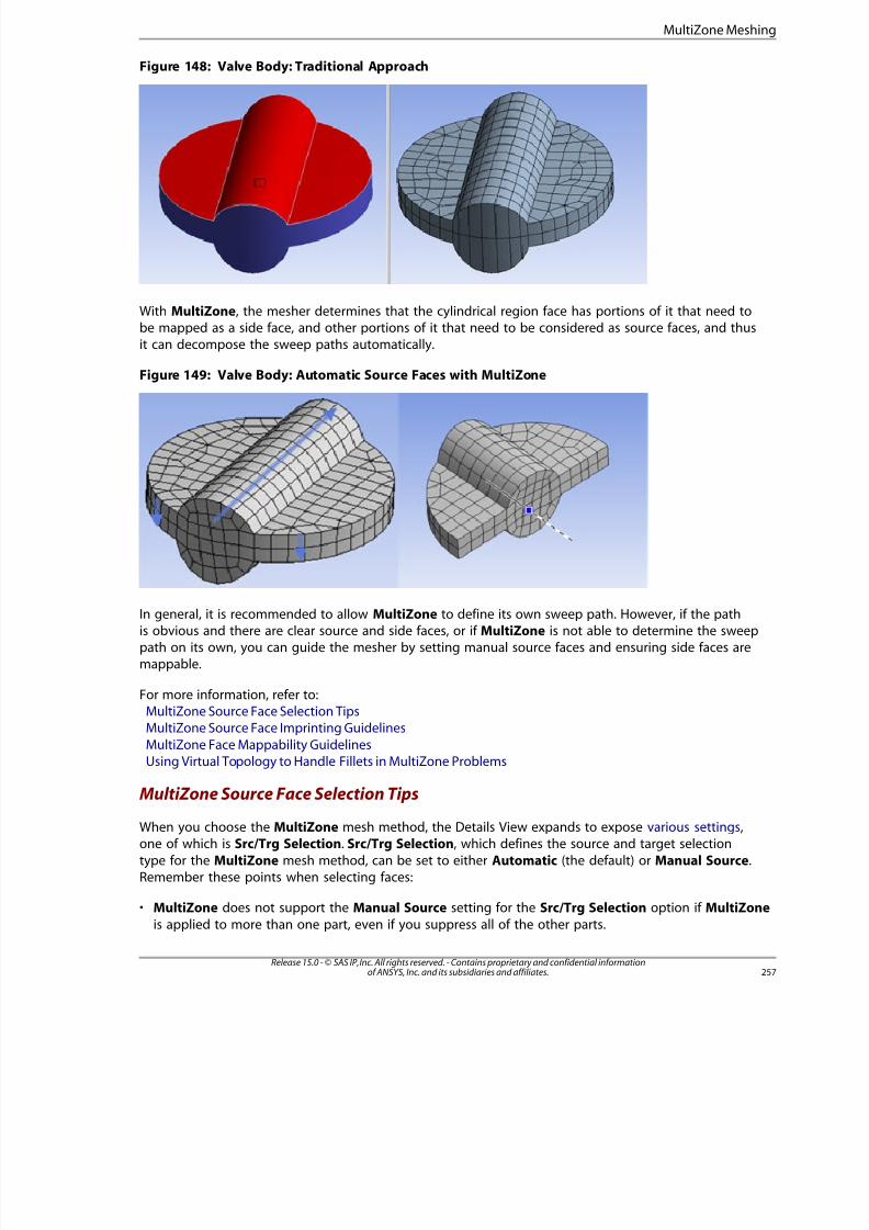
8/10/2019 ANSYS Meshing Users Guide
http://slidepdf.com/reader/full/ansys-meshing-users-guide 265/491
Figure 148: Valve Body: Traditional Approach
With MultiZone, the mesher determines that the cylindrical region face has portions of it that need tobe mapped as a side face, and other portions of it that need to be considered as source faces, and thusit can decompose the sweep paths automatically.
Figure 149: Valve Body: Automatic Source Faces with MultiZone
In general, it is recommended to allow MultiZone to define its own sweep path. However, if the pathis obvious and there are clear source and side faces, or if MultiZone is not able to determine the sweeppath on its own, you can guide the mesher by setting manual source faces and ensuring side faces aremappable.
For more information, refer to:MultiZone Source Face Selection TipsMultiZone Source Face Imprinting Guidelines
MultiZone Face Mappability GuidelinesUsing Virtual Topology to Handle Fillets in MultiZone Problems
MultiZone Source Face Selection Tips
When you choose the MultiZone mesh method, the Details View expands to expose various settings,one of which is Src/Trg Selection. Src/Trg Selection, which defines the source and target selection
type for the MultiZone mesh method, can be set to either Automatic (the default) or Manual Source.Remember these points when selecting faces:
• MultiZone does not support the Manual Source setting for the Src/Trg Selection option if MultiZone
is applied to more than one part, even if you suppress all of the other parts.
257Release 15.0 - © SAS IP, Inc. All rights reserved. - Contains proprietary and confidential informationof ANSYS, Inc. and its subsidiaries and affiliates.
MultiZone Meshing
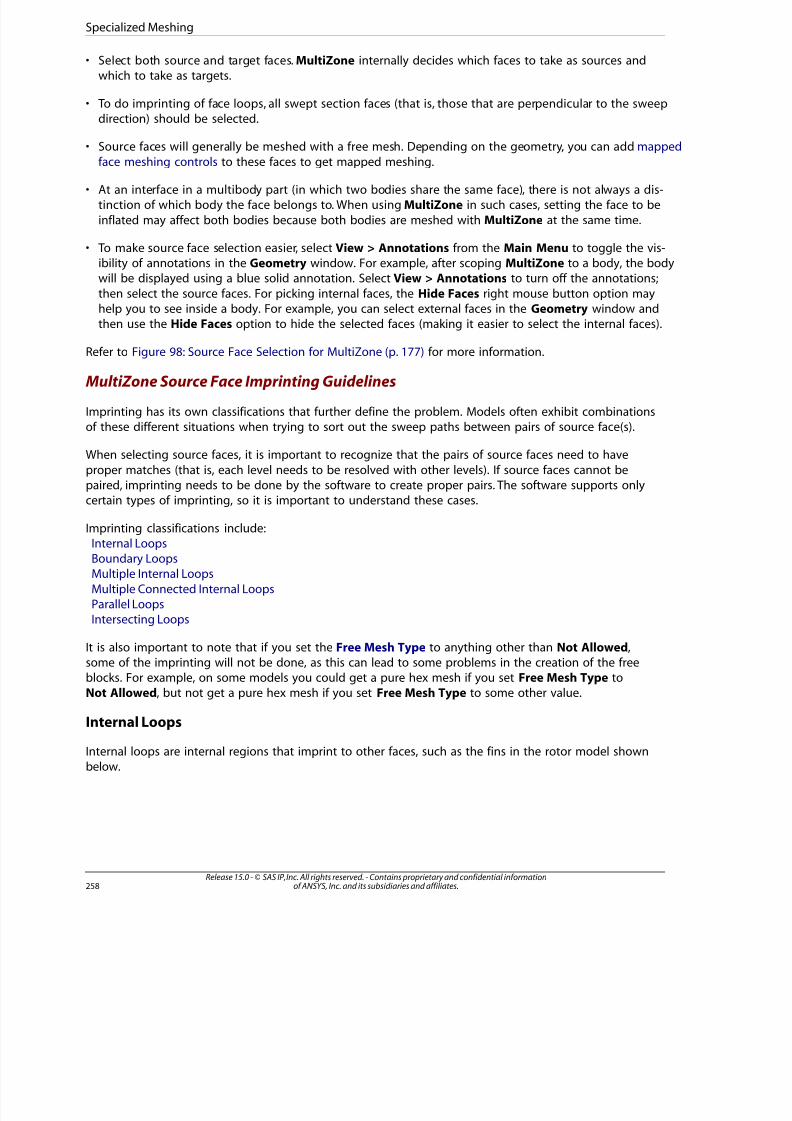
8/10/2019 ANSYS Meshing Users Guide
http://slidepdf.com/reader/full/ansys-meshing-users-guide 266/491
• Select both source and target faces. MultiZone internally decides which faces to take as sources andwhich to take as targets.
• To do imprinting of face loops, all swept section faces (that is, those that are perpendicular to the sweepdirection) should be selected.
• Source faces will generally be meshed with a free mesh. Depending on the geometry, you can add mapped
face meshing controls to these faces to get mapped meshing.
• At an interface in a multibody part (in which two bodies share the same face), there is not always a dis-tinction of which body the face belongs to. When using MultiZone in such cases, setting the face to be
inflated may affect both bodies because both bodies are meshed with MultiZone at the same time.
• To make source face selection easier, select View > Annotations from the Main Menu to toggle the vis-ibility of annotations in the Geometry window. For example, after scoping MultiZone to a body, the bodywill be displayed using a blue solid annotation. Select View > Annotations to turn off the annotations;
then select the source faces. For picking internal faces, the Hide Faces right mouse button option mayhelp you to see inside a body. For example, you can select external faces in the Geometry window andthen use the Hide Faces option to hide the selected faces (making it easier to select the internal faces).
Refer to Figure 98: Source Face Selection for MultiZone (p. 177) for more information.
MultiZone Source Face Imprinting Guidelines
Imprinting has its own classifications that further define the problem. Models often exhibit combinationsof these different situations when trying to sort out the sweep paths between pairs of source face(s).
When selecting source faces, it is important to recognize that the pairs of source faces need to have
proper matches (that is, each level needs to be resolved with other levels). If source faces cannot bepaired, imprinting needs to be done by the software to create proper pairs. The software supports onlycertain types of imprinting, so it is important to understand these cases.
Imprinting classifications include:Internal LoopsBoundary LoopsMultiple Internal Loops
Multiple Connected Internal LoopsParallel LoopsIntersecting Loops
It is also important to note that if you set the Free Mesh Type to anything other than Not Allowed,some of the imprinting will not be done, as this can lead to some problems in the creation of the freeblocks. For example, on some models you could get a pure hex mesh if you set Free Mesh Type toNot Allowed, but not get a pure hex mesh if you set Free Mesh Type to some other value.
Internal Loops
Internal loops are internal regions that imprint to other faces, such as the fins in the rotor model shownbelow.
Release 15.0 - © SAS IP, Inc. All rights reserved. - Contains proprietary and confidential informationof ANSYS, Inc. and its subsidiaries and affiliates.258
Specialized Meshing
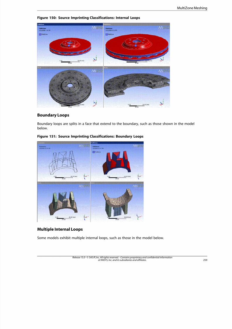
8/10/2019 ANSYS Meshing Users Guide
http://slidepdf.com/reader/full/ansys-meshing-users-guide 267/491
Figure 150: Source Imprinting Classifications: Internal Loops
Boundary Loops
Boundary loops are splits in a face that extend to the boundary, such as those shown in the modelbelow.
Figure 151: Source Imprinting Classifications: Boundary Loops
Multiple Internal Loops
Some models exhibit multiple internal loops, such as those in the model below.
259Release 15.0 - © SAS IP, Inc. All rights reserved. - Contains proprietary and confidential informationof ANSYS, Inc. and its subsidiaries and affiliates.
MultiZone Meshing
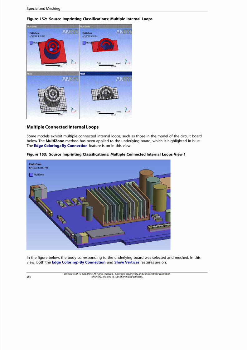
8/10/2019 ANSYS Meshing Users Guide
http://slidepdf.com/reader/full/ansys-meshing-users-guide 268/491
Figure 152: Source Imprinting Classifications: Multiple Internal Loops
Multiple Connected Internal Loops
Some models exhibit multiple connected internal loops, such as those in the model of the circuit boardbelow. The MultiZone method has been applied to the underlying board, which is highlighted in blue.
The Edge Coloring>By Connection feature is on in this view.
Figure 153: Source Imprinting Classifications: Multiple Connected Internal Loops View 1
In the figure below, the body corresponding to the underlying board was selected and meshed. In thisview, both the Edge Coloring>By Connection and Show Vertices features are on.
Release 15.0 - © SAS IP, Inc. All rights reserved. - Contains proprietary and confidential informationof ANSYS, Inc. and its subsidiaries and affiliates.260
Specialized Meshing
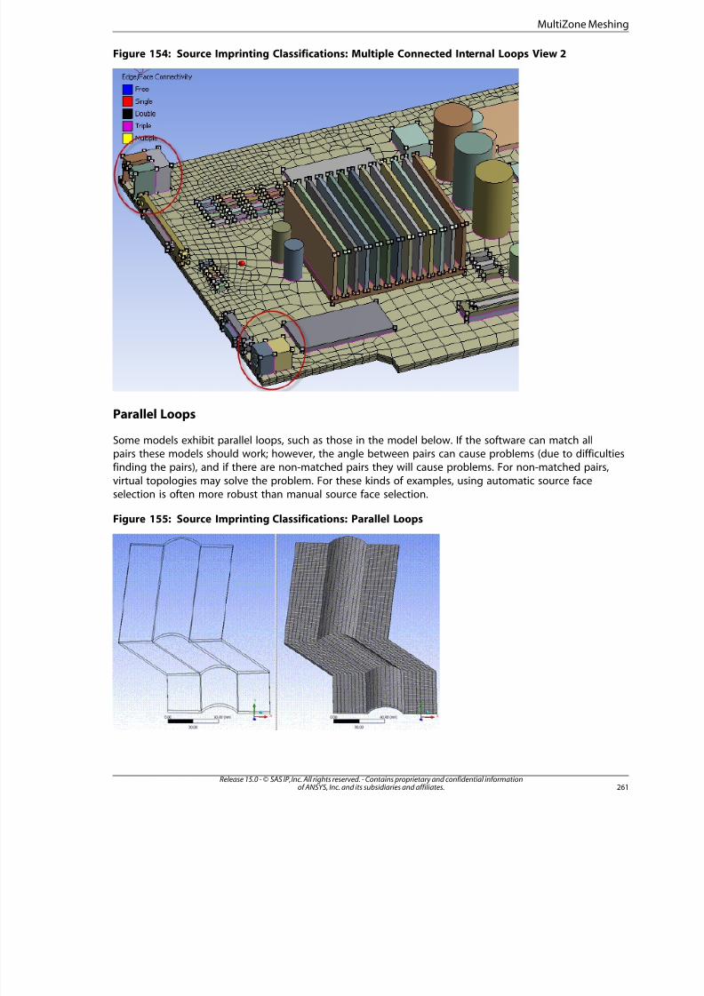
8/10/2019 ANSYS Meshing Users Guide
http://slidepdf.com/reader/full/ansys-meshing-users-guide 269/491
Figure 154: Source Imprinting Classifications: Multiple Connected Internal Loops View 2
Parallel Loops
Some models exhibit parallel loops, such as those in the model below. If the software can match allpairs these models should work; however, the angle between pairs can cause problems (due to difficulties
finding the pairs), and if there are non-matched pairs they will cause problems. For non-matched pairs,virtual topologies may solve the problem. For these kinds of examples, using automatic source faceselection is often more robust than manual source face selection.
Figure 155: Source Imprinting Classifications: Parallel Loops
26Release 15.0 - © SAS IP, Inc. All rights reserved. - Contains proprietary and confidential informationof ANSYS, Inc. and its subsidiaries and affiliates.
MultiZone Meshing
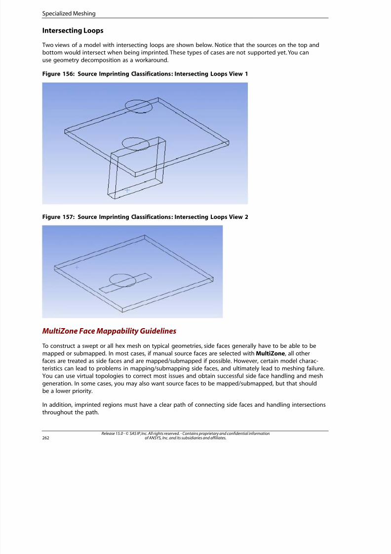
8/10/2019 ANSYS Meshing Users Guide
http://slidepdf.com/reader/full/ansys-meshing-users-guide 270/491
Intersecting Loops
Two views of a model with intersecting loops are shown below. Notice that the sources on the top andbottom would intersect when being imprinted. These types of cases are not supported yet. You can
use geometry decomposition as a workaround.
Figure 156: Source Imprinting Classifications: Intersecting Loops View 1
Figure 157: Source Imprinting Classifications: Intersecting Loops View 2
MultiZone Face Mappability Guidelines
To construct a swept or all hex mesh on typical geometries, side faces generally have to be able to bemapped or submapped. In most cases, if manual source faces are selected with MultiZone, all otherfaces are treated as side faces and are mapped/submapped if possible. However, certain model charac-teristics can lead to problems in mapping/submapping side faces, and ultimately lead to meshing failure.You can use virtual topologies to correct most issues and obtain successful side face handling and mesh
generation. In some cases, you may also want source faces to be mapped/submapped, but that shouldbe a lower priority.
In addition, imprinted regions must have a clear path of connecting side faces and handling intersections
throughout the path.
Release 15.0 - © SAS IP, Inc. All rights reserved. - Contains proprietary and confidential informationof ANSYS, Inc. and its subsidiaries and affiliates.262
Specialized Meshing
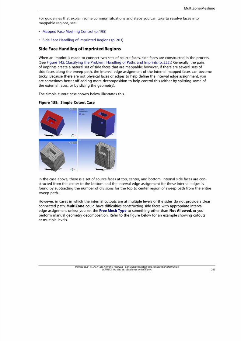
8/10/2019 ANSYS Meshing Users Guide
http://slidepdf.com/reader/full/ansys-meshing-users-guide 271/491
For guidelines that explain some common situations and steps you can take to resolve faces intomappable regions, see:
• Mapped Face Meshing Control (p. 195)
• Side Face Handling of Imprinted Regions (p. 263)
Side Face Handling of Imprinted Regions
When an imprint is made to connect two sets of source faces, side faces are constructed in the process.
(See Figure 145: Classifying the Problem: Handling of Paths and Imprints (p. 255).) Generally, the pairsof imprints create a natural set of side faces that are mappable; however, if there are several sets of side faces along the sweep path, the interval edge assignment of the internal mapped faces can become
tricky. Because there are not physical faces or edges to help define the interval edge assignment, youare sometimes better off adding more decomposition to help control this (either by splitting some of the external faces, or by slicing the geometry).
The simple cutout case shown below illustrates this.
Figure 158: Simple Cutout Case
In the case above, there is a set of source faces at top, center, and bottom. Internal side faces are con-structed from the center to the bottom and the interval edge assignment for these internal edges isfound by subtracting the number of divisions for the top to center region of sweep path from the entiresweep path.
However, in cases in which the internal cutouts are at multiple levels or the sides do not provide a clearconnected path, MultiZone could have difficulties constructing side faces with appropriate intervaledge assignment unless you set the Free Mesh Type to something other than Not Allowed, or you
perform manual geometry decomposition. Refer to the figure below for an example showing cutoutsat multiple levels.
263Release 15.0 - © SAS IP, Inc. All rights reserved. - Contains proprietary and confidential informationof ANSYS, Inc. and its subsidiaries and affiliates.
MultiZone Meshing
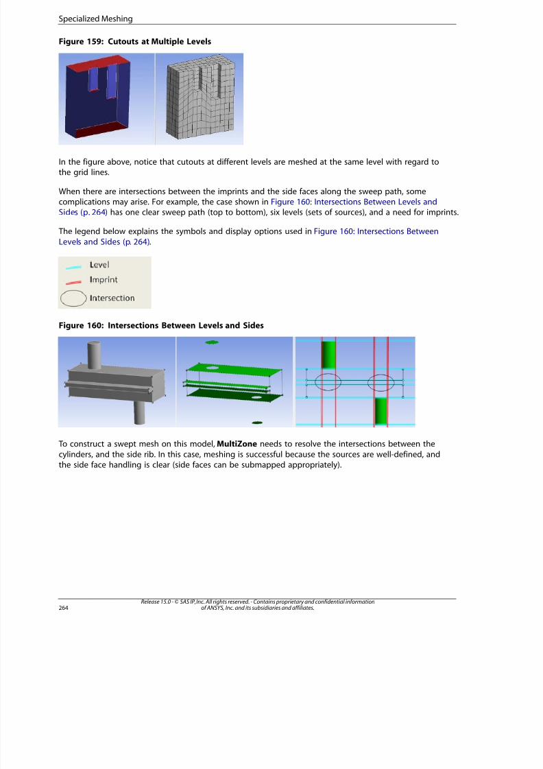
8/10/2019 ANSYS Meshing Users Guide
http://slidepdf.com/reader/full/ansys-meshing-users-guide 272/491
Figure 159: Cutouts at Multiple Levels
In the figure above, notice that cutouts at different levels are meshed at the same level with regard tothe grid lines.
When there are intersections between the imprints and the side faces along the sweep path, somecomplications may arise. For example, the case shown in Figure 160: Intersections Between Levels andSides (p. 264) has one clear sweep path (top to bottom), six levels (sets of sources), and a need for imprints.
The legend below explains the symbols and display options used in Figure 160: Intersections Between
Levels and Sides (p. 264).
Figure 160: Intersections Between Levels and Sides
To construct a swept mesh on this model, MultiZone needs to resolve the intersections between the
cylinders, and the side rib. In this case, meshing is successful because the sources are well-defined, andthe side face handling is clear (side faces can be submapped appropriately).
Release 15.0 - © SAS IP, Inc. All rights reserved. - Contains proprietary and confidential informationof ANSYS, Inc. and its subsidiaries and affiliates.264
Specialized Meshing
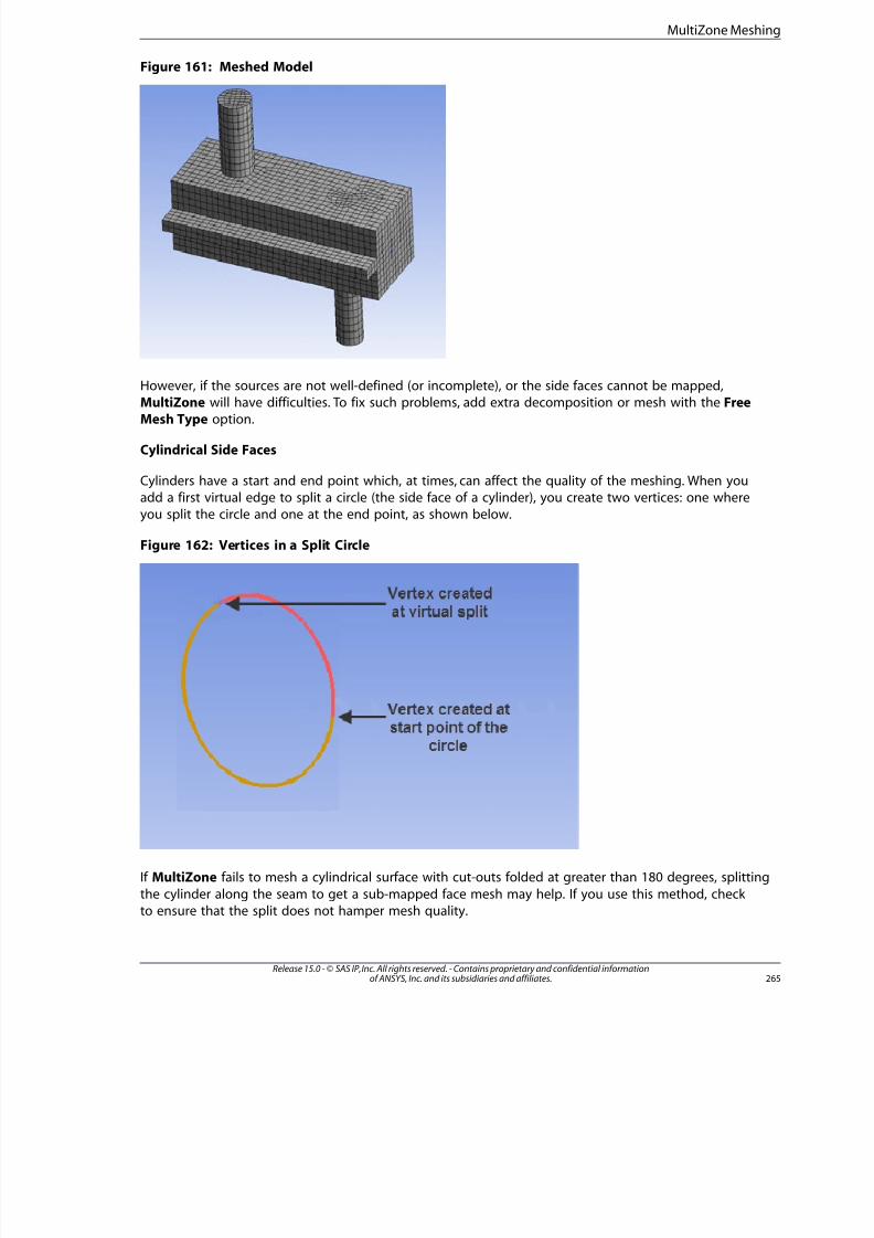
8/10/2019 ANSYS Meshing Users Guide
http://slidepdf.com/reader/full/ansys-meshing-users-guide 273/491
Figure 161: Meshed Model
However, if the sources are not well-defined (or incomplete), or the side faces cannot be mapped,MultiZone will have difficulties. To fix such problems, add extra decomposition or mesh with the FreeMesh Type option.
Cylindrical Side Faces
Cylinders have a start and end point which, at times, can affect the quality of the meshing. When youadd a first virtual edge to split a circle (the side face of a cylinder), you create two vertices: one whereyou split the circle and one at the end point, as shown below.
Figure 162: Vertices in a Split Circle
If MultiZone fails to mesh a cylindrical surface with cut-outs folded at greater than 180 degrees, splitting
the cylinder along the seam to get a sub-mapped face mesh may help. If you use this method, check to ensure that the split does not hamper mesh quality.
265Release 15.0 - © SAS IP, Inc. All rights reserved. - Contains proprietary and confidential informationof ANSYS, Inc. and its subsidiaries and affiliates.
MultiZone Meshing
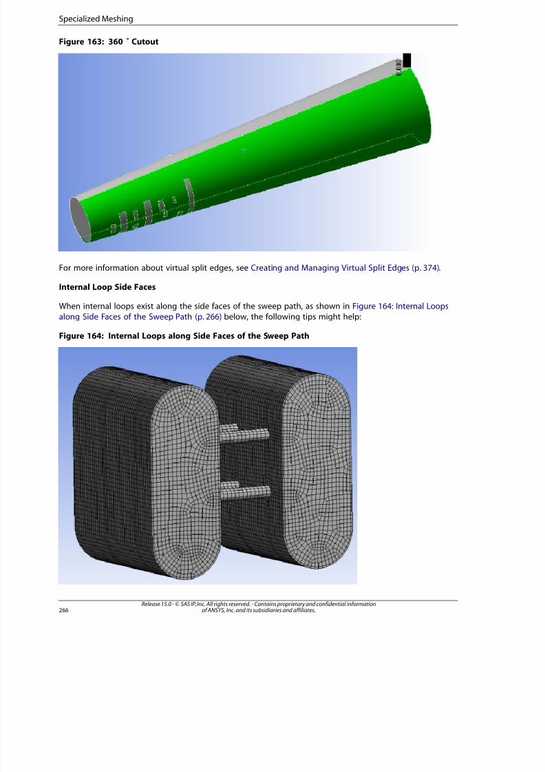
8/10/2019 ANSYS Meshing Users Guide
http://slidepdf.com/reader/full/ansys-meshing-users-guide 274/491
Figure 163: 360 ˚ Cutout
For more information about virtual split edges, see Creating and Managing Virtual Split Edges (p. 374).
Internal Loop Side Faces
When internal loops exist along the side faces of the sweep path, as shown in Figure 164: Internal Loops
along Side Faces of the Sweep Path (p. 266) below, the following tips might help:
Figure 164: Internal Loops along Side Faces of the Sweep Path
Release 15.0 - © SAS IP, Inc. All rights reserved. - Contains proprietary and confidential informationof ANSYS, Inc. and its subsidiaries and affiliates.266
Specialized Meshing
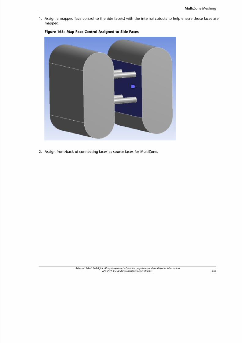
8/10/2019 ANSYS Meshing Users Guide
http://slidepdf.com/reader/full/ansys-meshing-users-guide 275/491
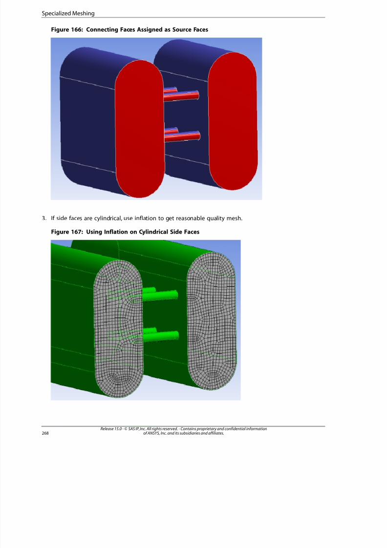
8/10/2019 ANSYS Meshing Users Guide
http://slidepdf.com/reader/full/ansys-meshing-users-guide 276/491
Figure 166: Connecting Faces Assigned as Source Faces
3. If side faces are cylindrical, use inflation to get reasonable quality mesh.
Figure 167: Using Inflation on Cylindrical Side Faces
Release 15.0 - © SAS IP, Inc. All rights reserved. - Contains proprietary and confidential informationof ANSYS, Inc. and its subsidiaries and affiliates.268
Specialized Meshing
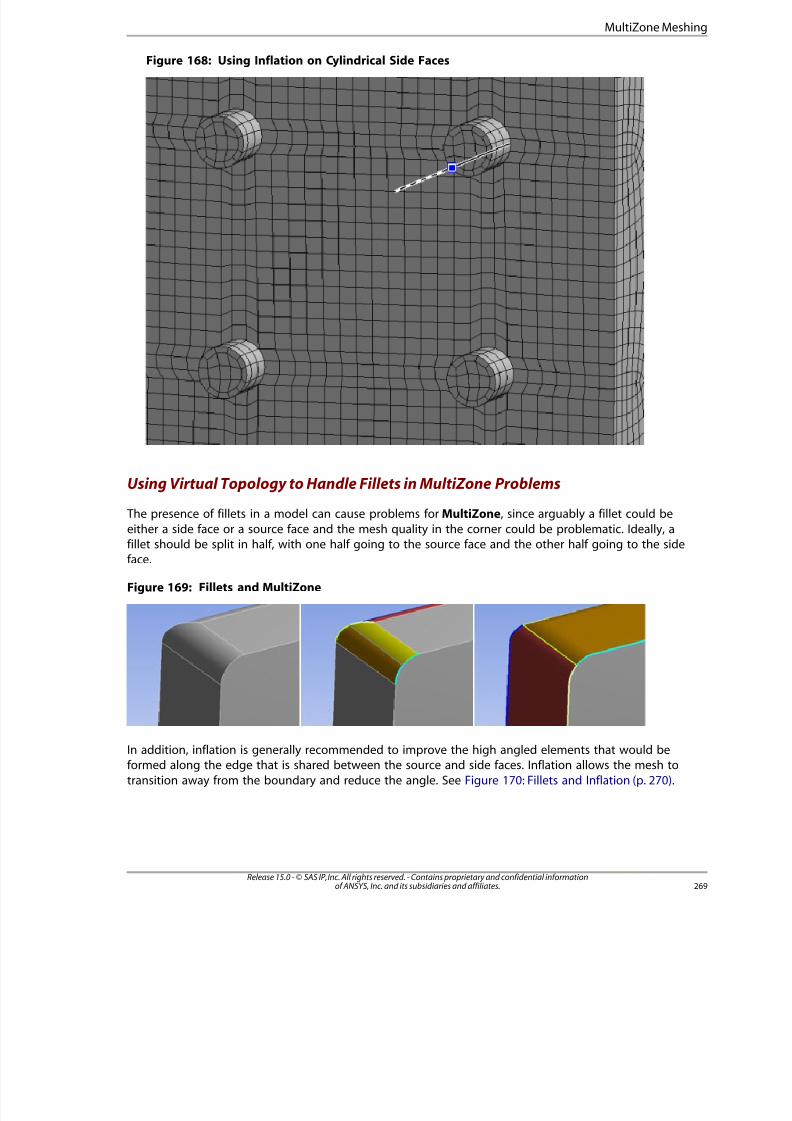
8/10/2019 ANSYS Meshing Users Guide
http://slidepdf.com/reader/full/ansys-meshing-users-guide 277/491
Figure 168: Using Inflation on Cylindrical Side Faces
Using Virtual Topology to Handle Fillets in MultiZone Problems
The presence of fillets in a model can cause problems for MultiZone, since arguably a fillet could be
either a side face or a source face and the mesh quality in the corner could be problematic. Ideally, afillet should be split in half, with one half going to the source face and the other half going to the sideface.
Figure 169: Fillets and MultiZone
In addition, inflation is generally recommended to improve the high angled elements that would beformed along the edge that is shared between the source and side faces. Inflation allows the mesh to
transition away from the boundary and reduce the angle. See Figure 170: Fillets and Inflation (p. 270).
269Release 15.0 - © SAS IP, Inc. All rights reserved. - Contains proprietary and confidential informationof ANSYS, Inc. and its subsidiaries and affiliates.
MultiZone Meshing
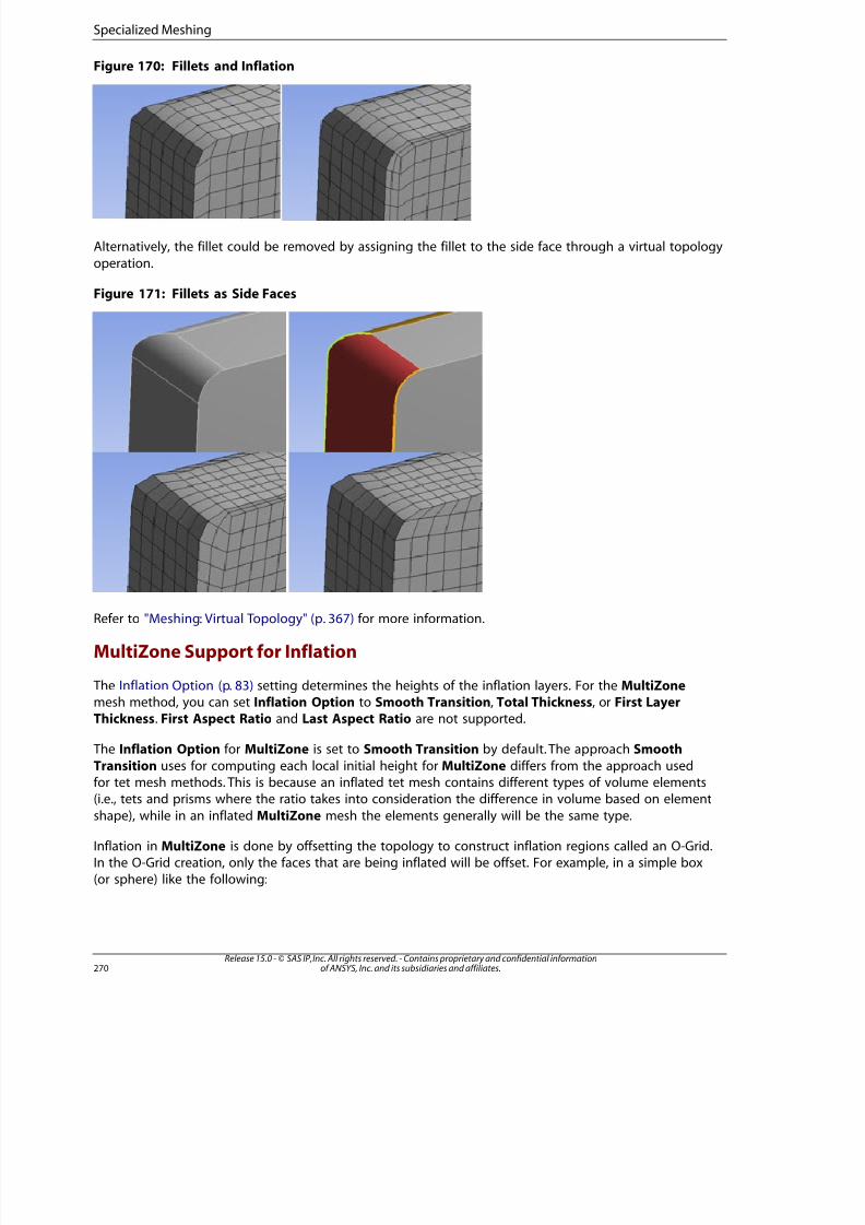
8/10/2019 ANSYS Meshing Users Guide
http://slidepdf.com/reader/full/ansys-meshing-users-guide 278/491
Figure 170: Fillets and Inflation
Alternatively, the fillet could be removed by assigning the fillet to the side face through a virtual topology
operation.
Figure 171: Fillets as Side Faces
Refer to "Meshing: Virtual Topology" (p. 367) for more information.
MultiZone Support for Inflation
The Inflation Option (p. 83) setting determines the heights of the inflation layers. For the MultiZonemesh method, you can set Inflation Option to Smooth Transition, Total Thickness, or First LayerThickness. First Aspect Ratio and Last Aspect Ratio are not supported.
The Inflation Option for MultiZone is set to Smooth Transition by default. The approach Smooth
Transition uses for computing each local initial height for MultiZone differs from the approach usedfor tet mesh methods. This is because an inflated tet mesh contains different types of volume elements(i.e., tets and prisms where the ratio takes into consideration the difference in volume based on element
shape), while in an inflated MultiZone mesh the elements generally will be the same type.
Inflation in MultiZone is done by offsetting the topology to construct inflation regions called an O-Grid.In the O-Grid creation, only the faces that are being inflated will be offset. For example, in a simple box(or sphere) like the following:
Release 15.0 - © SAS IP, Inc. All rights reserved. - Contains proprietary and confidential informationof ANSYS, Inc. and its subsidiaries and affiliates.270
Specialized Meshing
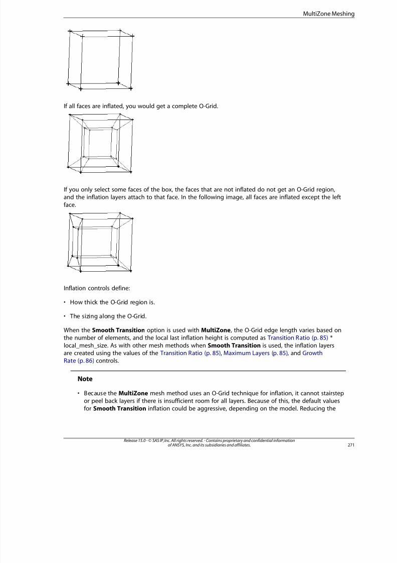
8/10/2019 ANSYS Meshing Users Guide
http://slidepdf.com/reader/full/ansys-meshing-users-guide 279/491
If all faces are inflated, you would get a complete O-Grid.
If you only select some faces of the box, the faces that are not inflated do not get an O-Grid region,and the inflation layers attach to that face. In the following image, all faces are inflated except the left
face.
Inflation controls define:
• How thick the O-Grid region is.
• The sizing along the O-Grid.
When the Smooth Transition option is used with MultiZone, the O-Grid edge length varies based onthe number of elements, and the local last inflation height is computed as Transition Ratio (p. 85) *
local_mesh_size. As with other mesh methods when Smooth Transition is used, the inflation layers
are created using the values of the Transition Ratio (p. 85), Maximum Layers (p. 85), and GrowthRate (p. 86) controls.
Note
• Because the MultiZone mesh method uses an O-Grid technique for inflation, it cannot stairstepor peel back layers if there is insufficient room for all layers. Because of this, the default valuesfor Smooth Transition inflation could be aggressive, depending on the model. Reducing the
27Release 15.0 - © SAS IP, Inc. All rights reserved. - Contains proprietary and confidential informationof ANSYS, Inc. and its subsidiaries and affiliates.
MultiZone Meshing
8/10/2019 ANSYS Meshing Users Guide
http://slidepdf.com/reader/full/ansys-meshing-users-guide 280/491
number of layers or switching to a different type of inflation definition may be more suitablefor some models.
• MultiZone supports Program Controlled (p. 81) inflation.
• The Collision Avoidance (p. 90) option is not used for MultiZone as the inflation layers arecreated within the blocking approach.
MultiZone Limitations and Hints
Be aware of the following limitations and hints when using MultiZone:
• Advanced mapped face meshing controls (side/end/corner) are not supported.
• Pinch controls are not supported.
• Only three-dimensional bodies can be used as Bodies of Influence (BOIs).
• The hard-sizing behavior of Sphere of influence (SOI) controls is not supported; you can define a re-finement with an SOI control but not a coarsening. The SOI element size is only applicable in the meshif it is smaller than the local mesh size without SOI.
• BOI controls are interpreted as an agglomerate of SOI controls that fill the body of influence. Therefore,on the boundaries of that body, the size might be a little larger because the location is not in oneof the spheres.
• The scope is not used for the SOI/BOI definition. The SOI/BOI does not act only on the scoped topology,
but on all topologies within the region of the SOI/BOI.
• In MultiZone, a closed edge is represented by more than one blocking topological edges. Therefore,
user-specified edge node distribution size may not be respected. However, the number of intervalswill still be respected,
• For split curves in rotated edge association, only interval count, not distribution, will be respected.
• Some inflation cases are not supported; for example, when the inflation does not form a closed loop
(which would lead to non-conformal mesh that is not allowed). In these cases the inflation will beskipped. Also see MultiZone Support for Inflation (p. 270).
• The Show Sweepable Bodies feature is a good tool to detect bodies that should mesh with MultiZone.
• There is no access to underlying blocks except by writing out the ANSYS ICEM CFD files.
• For help in diagnosing problems when using the MultiZone method, refer to the description of theEdge Graphics Options toolbar in the Mechanical help. This toolbar provides access to features thatare intended to improve your ability to distinguish edge and mesh connectivity.
• See Handling General MultiZone Meshing Failures (p. 398) for more information.
For additional information, refer to Interactions Between Mesh Methods and Mesh Controls (p. 348)(Patch Independent Mesh Methods table).
Release 15.0 - © SAS IP, Inc. All rights reserved. - Contains proprietary and confidential informationof ANSYS, Inc. and its subsidiaries and affiliates.272
Specialized Meshing

8/10/2019 ANSYS Meshing Users Guide
http://slidepdf.com/reader/full/ansys-meshing-users-guide 281/491
Assembly Meshing
Two algorithms are available for assembly meshing:
• CutCell
• Tetrahedrons
CutCell Cartesian meshing is a general purpose meshing method designed for ANSYS Fluent. The Tet-rahedrons assembly meshing algorithm is a derivative of the CutCell algorithm, with strengths andweaknesses similar to those of CutCell. The Tetrahedrons method starts from the CutCell mesh and
through various mesh manipulations creates a high quality unstructured tet mesh.
The CutCell method uses a patch independent volume meshing approach (surface mesh automaticallycreated from boundary of volume mesh) without the need for manual geometry cleanup or decompos-ition, thereby reducing the turnaround time required for meshing. The CutCell method is useful for
meshing fluid bodies in single body parts and multibody parts and assemblies of unconnected solids;it cannot be used to mesh a collection of loosely closed surface patches.
The CutCell algorithm is suitable for a large range of applications, and due to the large fraction of hex
cells in the mesh, often produces better results than tetrahedral methods.
CutCell is supported in the Meshing application only. The Tetrahedrons algorithm is available in boththe Meshing application and the Mechanical application; however, meshes generated using assembly
meshing are not supported for Mechanical solvers. Refer to Method (p. 97) for details.
Assembly meshing topics include: The Assembly Meshing Process The Assembly Meshing Workflow
The Assembly Meshing Process
The assembly meshing process involves the following approach:
1. Size functions and virtual bodies (optional) are defined.
Note
You can define virtual bodies to represent flow volumes if your model does notcontain a “solid” that represents the fluid region. In this way, virtual bodies allow
you to mesh fluid regions without having to use the DesignModeler application oranother solid modeler to model them. The Fluid/Solid material property for virtualbodies is always set to Fluid (read-only).
2. The initial size of the Cartesian grid is computed based on the minimum and maximum size set for
the size functions.
3. A uniform Cartesian grid is created within the bounding box for the geometry.
4. The size function values are computed and the grid is then adaptively refined based on the local
size function values.
273Release 15.0 - © SAS IP, Inc. All rights reserved. - Contains proprietary and confidential informationof ANSYS, Inc. and its subsidiaries and affiliates.
Assembly Meshing
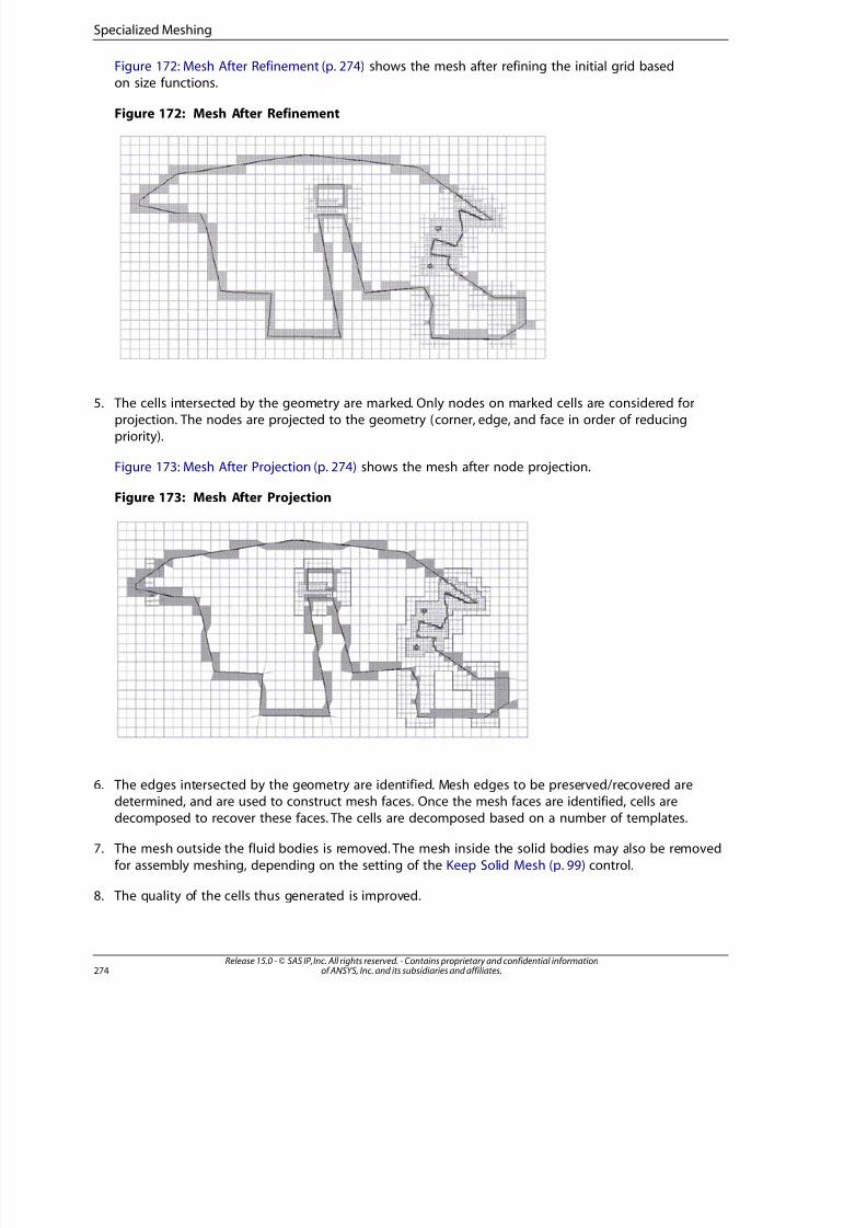
8/10/2019 ANSYS Meshing Users Guide
http://slidepdf.com/reader/full/ansys-meshing-users-guide 282/491
Figure 172: Mesh After Refinement (p. 274) shows the mesh after refining the initial grid basedon size functions.
Figure 172: Mesh After Refinement
5. The cells intersected by the geometry are marked. Only nodes on marked cells are considered forprojection. The nodes are projected to the geometry (corner, edge, and face in order of reducingpriority).
Figure 173: Mesh After Projection (p. 274) shows the mesh after node projection.
Figure 173: Mesh After Projection
6. The edges intersected by the geometry are identified. Mesh edges to be preserved/recovered aredetermined, and are used to construct mesh faces. Once the mesh faces are identified, cells aredecomposed to recover these faces. The cells are decomposed based on a number of templates.
7. The mesh outside the fluid bodies is removed. The mesh inside the solid bodies may also be removed
for assembly meshing, depending on the setting of the Keep Solid Mesh (p. 99) control.
8. The quality of the cells thus generated is improved.
Release 15.0 - © SAS IP, Inc. All rights reserved. - Contains proprietary and confidential informationof ANSYS, Inc. and its subsidiaries and affiliates.274
Specialized Meshing
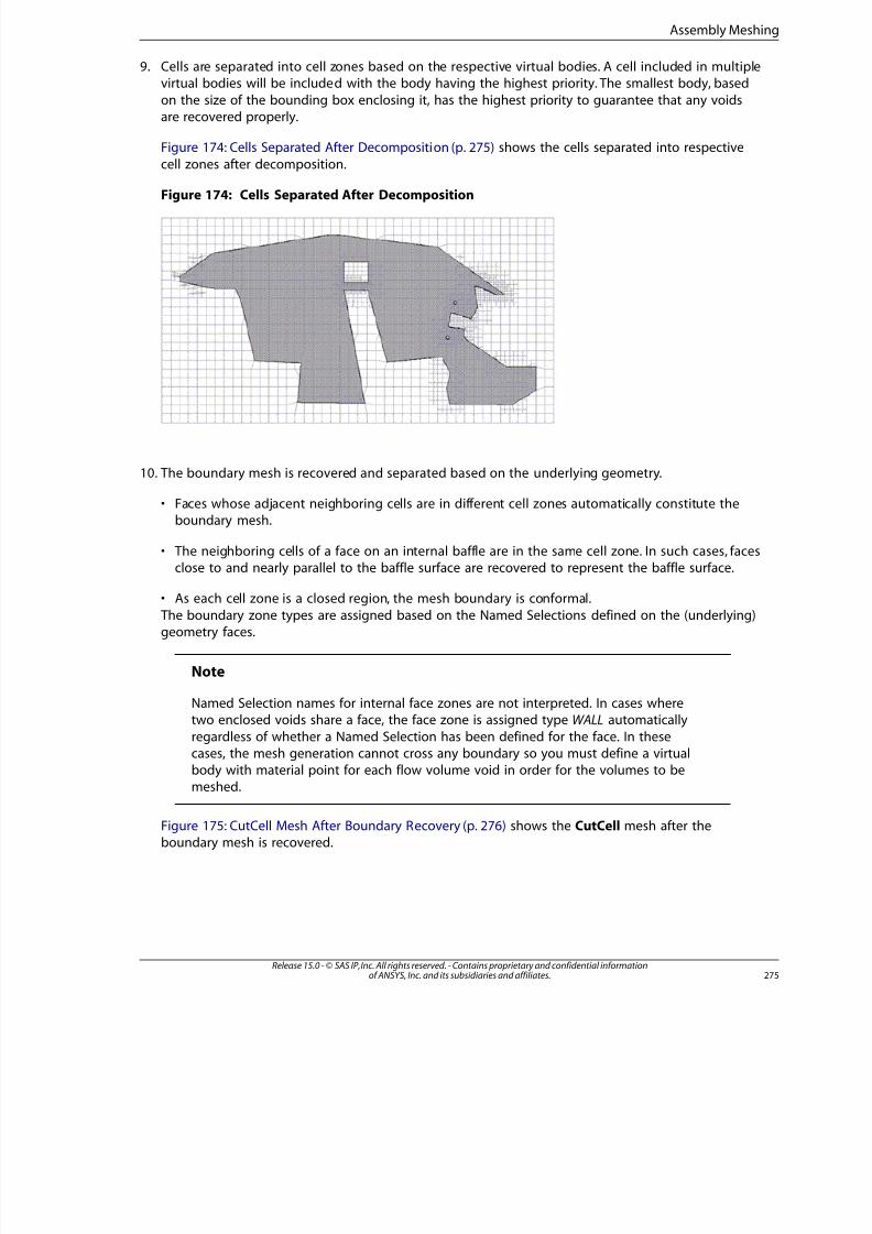
8/10/2019 ANSYS Meshing Users Guide
http://slidepdf.com/reader/full/ansys-meshing-users-guide 283/491
9. Cells are separated into cell zones based on the respective virtual bodies. A cell included in multiplevirtual bodies will be included with the body having the highest priority. The smallest body, based
on the size of the bounding box enclosing it, has the highest priority to guarantee that any voidsare recovered properly.
Figure 174: Cells Separated After Decomposition (p. 275) shows the cells separated into respective
cell zones after decomposition.
Figure 174: Cells Separated After Decomposition
10. The boundary mesh is recovered and separated based on the underlying geometry.
• Faces whose adjacent neighboring cells are in different cell zones automatically constitute theboundary mesh.
• The neighboring cells of a face on an internal baffle are in the same cell zone. In such cases, facesclose to and nearly parallel to the baffle surface are recovered to represent the baffle surface.
• As each cell zone is a closed region, the mesh boundary is conformal.
The boundary zone types are assigned based on the Named Selections defined on the (underlying)geometry faces.
Note
Named Selection names for internal face zones are not interpreted. In cases wheretwo enclosed voids share a face, the face zone is assigned type WALL automatically
regardless of whether a Named Selection has been defined for the face. In thesecases, the mesh generation cannot cross any boundary so you must define a virtual
body with material point for each flow volume void in order for the volumes to bemeshed.
Figure 175: CutCell Mesh After Boundary Recovery (p. 276) shows the CutCell mesh after theboundary mesh is recovered.
275Release 15.0 - © SAS IP, Inc. All rights reserved. - Contains proprietary and confidential informationof ANSYS, Inc. and its subsidiaries and affiliates.
Assembly Meshing

8/10/2019 ANSYS Meshing Users Guide
http://slidepdf.com/reader/full/ansys-meshing-users-guide 284/491
Figure 175: CutCell Mesh After Boundary Recovery
When the mesh is exported to ANSYS Fluent, a cell zone type of either FLUID or SOLID is assignedto each body based on its material properties. Refer to Fluent Mesh Export (p. 24) for details.
For information about material properties and which faces are selected to be inflation bound-
aries when Program Controlled inflation is defined for assembly meshing, refer to ProgramControlled (p. 81).
11. If the Tetrahedrons assembly meshing algorithm was selected, tet meshing extensions are applied. The Tetrahedrons algorithm starts with the CutCell mesh and transforms it into an unstructuredtet mesh.
The Assembly Meshing Workflow
This section describes the workflow for using assembly meshing, which is different from the workflowfor the other Meshing application mesh methods. Rather than being applied locally through insertionof a mesh method control, assembly meshing is a global operation as implied by its name and cannot
be used in combination with other meshing methods.
The general workflow for assembly meshing is as follows:
1. Set prerequisites.
2. Select an assembly mesh method (CutCell or Tetrahedrons).
3. Change Fluid/Solid material property settings (optional).
4. Define virtual bodies (optional).
5. Define mesh groups (optional).
Release 15.0 - © SAS IP, Inc. All rights reserved. - Contains proprietary and confidential informationof ANSYS, Inc. and its subsidiaries and affiliates.276
Specialized Meshing
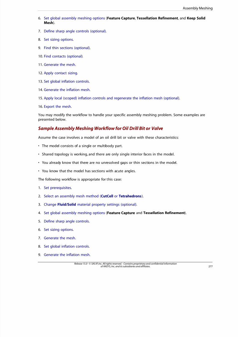
8/10/2019 ANSYS Meshing Users Guide
http://slidepdf.com/reader/full/ansys-meshing-users-guide 285/491
6. Set global assembly meshing options (Feature Capture, Tessellation Refinement, and Keep SolidMesh).
7. Define sharp angle controls (optional).
8. Set sizing options.
9. Find thin sections (optional).
10. Find contacts (optional).
11. Generate the mesh.
12. Apply contact sizing.
13. Set global inflation controls.
14. Generate the inflation mesh.
15. Apply local (scoped) inflation controls and regenerate the inflation mesh (optional) .
16. Export the mesh.
You may modify the workflow to handle your specific assembly meshing problem. Some examples arepresented below.
Sample Assembly Meshing Workflow for Oil Drill Bit or Valve
Assume the case involves a model of an oil drill bit or valve with these characteristics:
• The model consists of a single or multibody part.
• Shared topology is working, and there are only single interior faces in the model.
• You already know that there are no unresolved gaps or thin sections in the model.
• You know that the model has sections with acute angles.
The following workflow is appropriate for this case:
1. Set prerequisites.
2. Select an assembly mesh method (CutCell or Tetrahedrons).
3. Change Fluid/Solid material property settings (optional).
4. Set global assembly meshing options (Feature Capture and Tessellation Refinement).
5. Define sharp angle controls.
6. Set sizing options.
7. Generate the mesh.
8. Set global inflation controls.
9. Generate the inflation mesh.
277Release 15.0 - © SAS IP, Inc. All rights reserved. - Contains proprietary and confidential informationof ANSYS, Inc. and its subsidiaries and affiliates.
Assembly Meshing
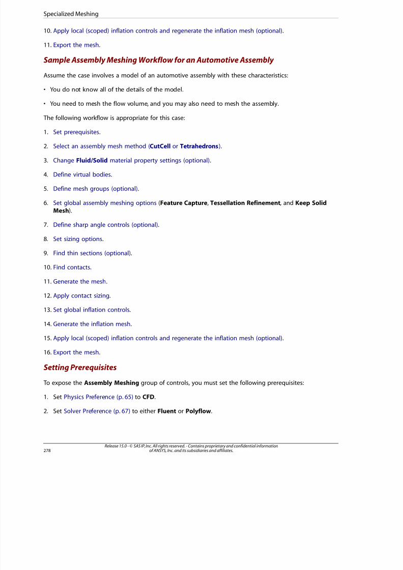
8/10/2019 ANSYS Meshing Users Guide
http://slidepdf.com/reader/full/ansys-meshing-users-guide 286/491
10. Apply local (scoped) inflation controls and regenerate the inflation mesh (optional) .
11. Export the mesh.
Sample Assembly Meshing Workflow for an Automotive Assembly
Assume the case involves a model of an automotive assembly with these characteristics:
• You do not know all of the details of the model.
• You need to mesh the flow volume, and you may also need to mesh the assembly.
The following workflow is appropriate for this case:
1. Set prerequisites.
2. Select an assembly mesh method (CutCell or Tetrahedrons).
3. Change Fluid/Solid material property settings (optional).
4. Define virtual bodies.
5. Define mesh groups (optional).
6. Set global assembly meshing options (Feature Capture, Tessellation Refinement, and Keep SolidMesh).
7. Define sharp angle controls (optional).
8. Set sizing options.
9. Find thin sections (optional).
10. Find contacts.
11. Generate the mesh.
12. Apply contact sizing.
13. Set global inflation controls.
14. Generate the inflation mesh.
15. Apply local (scoped) inflation controls and regenerate the inflation mesh (optional) .
16. Export the mesh.
Setting Prerequisites
To expose the Assembly Meshing group of controls, you must set the following prerequisites:
1. Set Physics Preference (p. 65) to CFD.
2. Set Solver Preference (p. 67) to either Fluent or Polyflow.
Release 15.0 - © SAS IP, Inc. All rights reserved. - Contains proprietary and confidential informationof ANSYS, Inc. and its subsidiaries and affiliates.278
Specialized Meshing
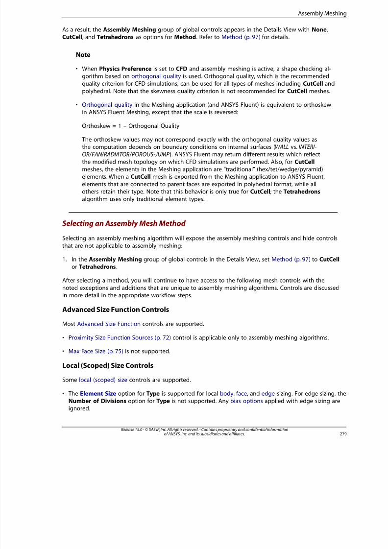
8/10/2019 ANSYS Meshing Users Guide
http://slidepdf.com/reader/full/ansys-meshing-users-guide 287/491
As a result, the Assembly Meshing group of global controls appears in the Details View with None,CutCell, and Tetrahedrons as options for Method. Refer to Method (p. 97) for details.
Note
• When Physics Preference is set to CFD and assembly meshing is active, a shape checking al-gorithm based on orthogonal quality is used. Orthogonal quality, which is the recommended
quality criterion for CFD simulations, can be used for all types of meshes including CutCell andpolyhedral. Note that the skewness quality criterion is not recommended for CutCell meshes.
• Orthogonal quality in the Meshing application (and ANSYS Fluent) is equivalent to orthoskewin ANSYS Fluent Meshing, except that the scale is reversed:
Orthoskew = 1 – Orthogonal Quality
The orthoskew values may not correspond exactly with the orthogonal quality values asthe computation depends on boundary conditions on internal surfaces (WALL vs. INTERI-
OR /FAN /RADIATOR /POROUS-JUMP ). ANSYS Fluent may return different results which reflect
the modified mesh topology on which CFD simulations are performed. Also, for CutCell
meshes, the elements in the Meshing application are “traditional” (hex/tet/wedge/pyramid)elements. When a CutCell mesh is exported from the Meshing application to ANSYS Fluent,
elements that are connected to parent faces are exported in polyhedral format, while allothers retain their type. Note that this behavior is only true for CutCell; the Tetrahedronsalgorithm uses only traditional element types.
Selecting an Assembly Mesh Method
Selecting an assembly meshing algorithm will expose the assembly meshing controls and hide controls
that are not applicable to assembly meshing:
1. In the Assembly Meshing group of global controls in the Details View, set Method (p. 97) to CutCellor Tetrahedrons.
After selecting a method, you will continue to have access to the following mesh controls with the
noted exceptions and additions that are unique to assembly meshing algorithms. Controls are discussedin more detail in the appropriate workflow steps.
Advanced Size Function Controls
Most Advanced Size Function controls are supported.
• Proximity Size Function Sources (p. 72) control is applicable only to assembly meshing algorithms.
• Max Face Size (p. 75) is not supported.
Local (Scoped) Size Controls
Some local (scoped) size controls are supported.
• The Element Size option for Type is supported for local body, face, and edge sizing. For edge sizing, theNumber of Divisions option for Type is not supported. Any bias options applied with edge sizing areignored.
279Release 15.0 - © SAS IP, Inc. All rights reserved. - Contains proprietary and confidential informationof ANSYS, Inc. and its subsidiaries and affiliates.
Assembly Meshing
8/10/2019 ANSYS Meshing Users Guide
http://slidepdf.com/reader/full/ansys-meshing-users-guide 288/491
• The Body of Influence option for Type is supported for local body sizing, but the body of influencecannot be scoped to a line body.
• If you want to use a body of influence with a virtual body, you can scope the body of influence to anybody in the geometry. The body of influence does not have to be inside or even in contact with thescoped body.
• The Sphere of Influence and Number of Divisions options for Type are not supported.
• No local vertex sizing is supported.
• Contact Sizing is supported. However, if contact sizing is applied to entities on a body that is scoped to
a body of influence, the contact sizing is ignored.
If any unsupported local size controls are defined prior to selection of an assembly meshing algorithm,they are suppressed when an assembly meshing algorithm is selected.
Inflation Controls
3D inflation controls are supported. This includes global (automatic Program Controlled) and local
(scoped) controls.
• A mixture of global and local inflation is not supported for assembly meshing algorithms. Consider thefollowing when determining whether to use global or local inflation:
– For inflation on virtual bodies, you must use automatic Program Controlled inflation; you cannot uselocal controls to inflate virtual bodies. Thus in general, if you are using virtual bodies to represent flowvolumes in your model, plan to use automatic inflation. Automatic inflation is specified globally by
setting Use Automatic Inflation (p. 80) to Program Controlled (p. 81). With Program Controlled inflation,faces on real solid bodies will inflate into the virtual bodies. The Fluid/Solid designation on real bodieswill be respected (that is, faces on real fluid bodies will inflate into the fluid region, but the solid regionwill not be inflated).
– Alternatively, you can set Use Automatic Inflation to None (p. 80) and define local inflation controls. This approach is appropriate if your model contains real bodies that represent the fluid regions.
The restriction from mixing global and local inflation results in the following behaviors:
– If Program Controlled inflation and local inflation are both defined and you select an assemblymeshing algorithm, Program Controlled inflation overrides the local inflation controls. The local inflationcontrols become inactive.
– If an assembly meshing algorithm is selected and local inflation is defined, the local inflation controlsbecome inactive if you select Program Controlled inflation.
– If an assembly meshing algorithm is selected and Program Controlled inflation is defined, the option
to insert local inflation will be grayed out (unavailable). You must set Use Automatic Inflation to Noneto be able to insert local inflation.
• By default, Inflation Option (p. 83) is set to Smooth Transition and Transition Ratio (p. 85) is set to 0.272.If you set Transition Ratio prior to selecting assembly meshing, your setting will be ignored for assembly
meshing but will be restored if you subsequently deselect assembly meshing and return to another meshmethod.
Release 15.0 - © SAS IP, Inc. All rights reserved. - Contains proprietary and confidential informationof ANSYS, Inc. and its subsidiaries and affiliates.280
Specialized Meshing

8/10/2019 ANSYS Meshing Users Guide
http://slidepdf.com/reader/full/ansys-meshing-users-guide 289/491
• The Inflation Algorithm (p. 87) control, which is used to select either the Pre or Post inflation algorithmfor other mesh methods, is hidden when an assembly meshing algorithm is selected.
For the CutCell algorithm, inflation is neither Pre nor Post. Rather, it may be considered a hybrid of the two, in that the technology used is like that of the Pre algorithm, but inflation occurs Post meshgeneration. For the Tetrahedrons algorithm, Pre inflation is used, with inflation behaviors and limit-
ations very similar to those of the Patch Conforming Tetrahedron mesh method.
If you set Inflation Algorithm prior to selecting an assembly meshing algorithm, your setting willbe ignored for assembly meshing but will be restored if you subsequently deselect assembly meshing
and return to another mesh method.
• Collision Avoidance (p. 90) is set to Layer Compression and is read-only. Note, however, that layercompression is used in areas of proximity and bad normals. In other problematic scenarios (for example,non-manifold nodes, bad surface mesh, and so on), local stair stepping is performed. As a result of local
stair stepping, poor quality cells may be introduced into the mesh. Because of this possibility, a warningmessage will appear whenever stair stepping occurs. The message will not identify the location of thestair stepping; however, it often coincides with the location of the worst quality cells. For this reason, usinthe Mesh Metric (p. 122) feature to locate the worst quality cells is also likely to locate the areas where
stair stepping occurred. To avoid stair stepping, make sure that the correct faces have been picked for
inflation and that small features are properly resolved, as stair stepping also may be related to bad resol-ution of acute angles.
• Inflation on baffles is supported for the Tetrahedrons algorithm only. Inflation can be applied to bafflesusing global (i.e., automatic Program Controlled (p. 81) inflation) or local controls. When Program Con-trolled inflation is used, baffles are automatically selected to be inflation boundaries unless they are parof a Named Selection (with the Program Controlled Inflation option set to Exclude). Only two-sided
growth cases for inflation are supported. Inflation layers will stair step at free boundary edges of thebaffles.
• By default, Gap Factor (p. 94) is set to 1.5 for the CutCell algorithm. For the Tetrahedrons algorithm,
Gap Factor is set equal to the value that is specified for non-assembly mesh methods ( 0.5 by default). The Gap Factor settings for the Tetrahedrons algorithm and the non-assembly mesh methods are syn-chronized such that if one is changed, the other is updated accordingly. However, changing the valuespecified for the CutCell algorithm has no effect on the value being used by the Tetrahedrons algorithm
and non-assembly mesh methods, and vice versa.
Gap Factor for the Tetrahedrons algorithm follows the same logic that is used by the Patch Con-forming Tetrahedrons mesh method.
If you are using an assembly meshing algorithm and the aspect ratio of cells in the inflation layerreaches 50, a warning message is issued. The warning message will suggest that you reduce the gapfactor, as doing so may improve the aspect ratio of these cells. Although reducing the gap factor
(e.g., a value of 0.5) may improve the quality, it may also have a negative impact on robustness. Ahigher value (e.g., 1.5) is generally more robust, but may not result in the best mesh quality.
• If you make changes to inflation settings after generating the mesh using an assembly meshing algoritheach subsequent re-mesh begins with the initial (cached) mesh and inflates from there.
Statistics Controls
Statistics controls are supported.
28Release 15.0 - © SAS IP, Inc. All rights reserved. - Contains proprietary and confidential informationof ANSYS, Inc. and its subsidiaries and affiliates.
Assembly Meshing
8/10/2019 ANSYS Meshing Users Guide
http://slidepdf.com/reader/full/ansys-meshing-users-guide 290/491
Virtual Topology
The use of virtual topology with assembly meshing is generally not recommended as it can lead to poorfaceting and thus poor feature capturing and/or mesh quality in assembly meshes. For these reasons,
a warning message is issued when virtual topologies are invoked with assembly meshing.
Unsupported Controls
Controls and features that are inaccessible when an assembly meshing algorithm is selected includethose listed below.
• The global Patch Conforming Options group of controls
• The global Advanced group of controls
• The global Defeaturing group of controls
• The following local (scoped) controls:
– Method
– Refinement
– Mapped Face Meshing
– Match
– Pinch
– 2D (face) Inflation
• Rigid bodies
• Symmetry—In the case of the Symmetry feature, it is accessible when an assembly meshing algorithm isselected but it will not be respected. If you attempt to use Symmetry with an assembly meshing algorithm,a warning message is issued.
• The following RMB menu options:
– Preview> Inflation
– Preview> Source and Target Mesh
– Preview> Surface Mesh
– Show> Mappable Faces
– Show> Program Controlled Inflation Surfaces
– Show> Removable Loops
Release 15.0 - © SAS IP, Inc. All rights reserved. - Contains proprietary and confidential informationof ANSYS, Inc. and its subsidiaries and affiliates.282
Specialized Meshing
8/10/2019 ANSYS Meshing Users Guide
http://slidepdf.com/reader/full/ansys-meshing-users-guide 291/491
– Show> Sweepable Bodies
Note
For supported mesh methods, the Preview Surface Mesh feature helps you to verify that
your mesh settings are correct by allowing you to visualize and examine the surface meshprior to generating the full mesh. The inaccessibility of Preview Surface Mesh for assembly
meshing does not present an obstacle for internal flow problems, as you can easily see themesh. However, since external flow problems involve a void, the following alternatives arerecommended:
• Use a Section Plane to look at the surface from the inside. This may be sufficient for simplemodels.
• For more complex models, define a Named Selection that includes all of the internalboundaries of the model, except those for which a Named Selection already exists. Youcan then view the surface mesh by viewing the Named Selection.
Changing Fluid/Solid Material Property Settings
You can use the Fluid/Solid material property setting to control the physics that will occur on a model:
1. Select a prototype (i.e., Body object) in the Tree Outline.
2. In the Details View, select the appropriate option for Fluid/Solid. Valid options are Fluid, Solid, andDefined By Geometry.
When set to Defined By Geometry, the value is based on the Fluid/Solid material property thatwas assigned to the body in the DesignModeler application.
Note
• Fluid/Solid also appears in the Details View if you select a Virtual Body object in the Tree
Outline, but in such cases it is always set to Fluid (read-only).
• Refer to Fluent Mesh Export (p. 24) for information about this setting and how material prop-erties are translated for use in ANSYS Fluent.
• Fluid/Solid is available in the Meshing application only; it is not available if you are using themeshing capabilities from within the Mechanical application.
Defining Virtual Bodies
Virtual bodies are supported for assembly meshing algorithms only. If your model does not contain a“solid” to represent a flow region, a virtual body can be defined so that you can mesh the flow region
without having to use the DesignModeler application or another solid modeler to model it. Virtualbodies are extremely beneficial in cases where it is not practical to extract flow volumes in a modeler. They can be defined by material point only, or by material point and a group of fluid surfaces.
283Release 15.0 - © SAS IP, Inc. All rights reserved. - Contains proprietary and confidential informationof ANSYS, Inc. and its subsidiaries and affiliates.
Assembly Meshing
8/10/2019 ANSYS Meshing Users Guide
http://slidepdf.com/reader/full/ansys-meshing-users-guide 292/491
As defined by a material point, the virtual body is an object that is defined by a coordinate systemrepresenting the origin of a material, and which extends from the origin until it reaches the face of
another solid (i.e., as when a ray is traced from the origin to the closest solid).
The two main reasons for using a group of fluid surfaces to help define a virtual body are performanceand mesh quality.
For example, consider a case involving a large assembly for which you want to analyze a small flow
volume but have no interest in the solid mesh. If you define the virtual body by material point only,assembly meshing refines and resolves every solid in the assembly, and finally, using mesh separation
and the material point, identifies the flow volume and discards the solid mesh. However, if you selecta group of fluid surfaces to help define the virtual body, assembly meshing resolves only the boundariesof the fluid surfaces in the group; essentially, it ignores all other boundaries. This approach typicallyspeeds up mesh generation by a factor of two or more.
With respect to mesh quality, using a group of fluid surfaces to help define a virtual body is a goodidea if you have a fluids-only problem (Keep Solid Mesh is set to No) where within the solids there are3D details and/or bodies that are smaller than the minimum size and hence would be problematic toresolve.
If fluid surface creation using the Extend to Connection option “leaks” to the outside of the domain,the leak needs to be closed. This approach provides an alternative way of detecting leaks. Extend toConnection is discussed in more detail below.
Note
• Virtual bodies and fluid surface objects are not supported when Meshing application capabilitiesare accessed from within the Mechanical application.
• A virtual body and the optional group of fluid surfaces that is used to help define it are repres-
ented in the Tree Outline by Virtual Body objects and Fluid Surface objects respectively. A
material point must be specified when a Fluid Surface object is being used to help define avirtual body. Both the Fluid Surface object and the Virtual Body object will remain under-defined until the material point is specified.
• The Fluid/Solid material property for a virtual body is always set to Fluid (read-only).
Defining a Virtual Body
The steps for defining a virtual body are presented here.
1. Select the Geometry object in the Tree Outline.
2. Insert a Virtual Body object into the Tree using either of these methods:
• Right-click on the Geometry object and select Insert > Virtual Body from the context menu.
Release 15.0 - © SAS IP, Inc. All rights reserved. - Contains proprietary and confidential informationof ANSYS, Inc. and its subsidiaries and affiliates.284
Specialized Meshing

8/10/2019 ANSYS Meshing Users Guide
http://slidepdf.com/reader/full/ansys-meshing-users-guide 293/491
• Choose Virtual Body on the Geometry context toolbar.
Note
If this is the first Virtual Body object to be inserted, a Virtual Body Group object will
be inserted into the Tree along with the Virtual Body object as its child object.
3. In the Details View, specify a value for Visible. The default is Yes. If set to No, the resultant mesh of thevirtual body will not appear in the Geometry window.
4. Specify a value for Suppressed. The default is No. If set to Yes, the virtual body will be suppressed andwill not be meshed, nor will it be sent to the solver if it is already meshed.
5. In the Details View, Used By Fluid Surface specifies whether the virtual body is being used by a group
of fluid surfaces. The default is No. If the virtual body will be used by a group of fluid surfaces, insert aFluid Surface object into the Tree by right-clicking on the Virtual Body object and selecting Insert >Fluid Surface from the context menu.
• Alternatively, you can change the setting to Yes in the Details View, and a new Fluid Surface objectwill be inserted under the Virtual Body object.
• Only one Fluid Surface object can be associated to any one Virtual Body object.
• If you switch the value of Used By Fluid Surface from Yes to No, the Fluid Surface object will be
hidden.
6. Click the Virtual Body object in the Tree to continue defining it. For Material Point, specify the coordisystem to be used for the virtual body, and the faces will be oriented accordingly. The default is Please
Define.
• The Fluid Surface object and Virtual Body object will remain underdefined until a material point isspecified.
• You can either select the default coordinate system or define a local coordinate system. In either cas
the setting will be retained, even if the Used By Fluid Surface setting is changed later.
The remaining fields for the virtual body are read-only:
• Fluid/Solid - Always set to Fluid for virtual bodies.
• Nodes, Elements, Mesh Metric - Data associated with the virtual body when meshed.
7. If Used By Fluid Surface is No, the definition of the virtual body is now complete. If the virtual body
will be used by a group of fluid surfaces (that is, Used By Fluid Surface is Yes), expand the Virtual Bodobject in the Tree Outline to expose the Fluid Surface object.
8. To define and make adjustments to the group of fluid surfaces, click the Fluid Surface object and usethe following controls. These controls appear in the Details View of the Fluid Surface object.
• Faces To Group: In the Geometry window, select the faces that should be members of the group.Refer to the example of the aero valve assembly below for information about automating face select
• Master Virtual Body: Read-only name of the master virtual body.
285Release 15.0 - © SAS IP, Inc. All rights reserved. - Contains proprietary and confidential informationof ANSYS, Inc. and its subsidiaries and affiliates.
Assembly Meshing

8/10/2019 ANSYS Meshing Users Guide
http://slidepdf.com/reader/full/ansys-meshing-users-guide 294/491
• Priority: Determines which group will claim cells in cases where groups overlap. The priority is initiallybased on the rule: the smaller the volume, the higher the priority.
• Suppressed: Read-only setting that is inherited from the virtual body.
Notes on Virtual Bodies
Remember the following information when defining virtual bodies:
• Connections are not supported.
• Statistics are supported.
• When coordinate systems are created they are represented in the Tree as objects named CoordinateSystem, Coordinate System 2, Coordinate System 3, and so on.
• Toggling the value of Used By Fluid Surface from Yes to No will result in the following behaviors:
– If you switch from Yes to No, the Fluid Surface object will be hidden.
– If you switch from No to Yes, the Fluid Surface object will be inserted into the Tree Outline, and the
virtual body will become the master body.
• If a group of fluid surfaces is being used to help define a virtual body, its suppression status is inheritedfrom the virtual body and is read-only.
• You should not use a group of fluid surfaces to help define a virtual body if one or more internal baffles(i.e., Surface Body with free edges) is located inside the flow volume void where you specified the mater-ial point. These baffles do not resolve properly in ANSYS Fluent.
• For flow volume extraction, make sure that capping faces have been created in your CAD package. Cappingfaces must be selected manually when defining virtual bodies. See Using the Extend to Connection Optionwith Fluid Surface Grouping (p. 290) for an example.
• Using one surface body to cap multiple inlets/outlets is not supported. Make sure that each opening is
capped with at least one face.
• The mesh around the edges of a capping surface must be properly resolved both by size and feature toensure that no leakage occurs.
• Contact sizing might be used to close gaps smaller than 1/4 of the minimum size. Note that contact sizingwill not properly recover features around the gap. Hence it is recommended to exclude inflation in thisarea.
• It is not recommended to use contact sizing to close a gap if faces in the connection are already included
in the sharp angle control.
• Contact sizing tools are not supported on baffle surfaces or capping surfaces.
• If you create a fluid body using Boolean operations from solid volumes, but shared topology fails, the re-commended action is to not use this geometry configuration in assembly meshing. Instead remove thefluid volumes and add a material point to extract the fluid volume inside meshing. Also see Handling of Interfaces Between Bodies in Assembly Meshing (p. 287).
• The Mesh cell state will go out-of-date and will require updating if:
Release 15.0 - © SAS IP, Inc. All rights reserved. - Contains proprietary and confidential informationof ANSYS, Inc. and its subsidiaries and affiliates.286
Specialized Meshing

8/10/2019 ANSYS Meshing Users Guide
http://slidepdf.com/reader/full/ansys-meshing-users-guide 295/491
– You suppress/unsuppress a virtual body.
– You delete a virtual body.
– You change the location of the material point that you selected for a virtual body.
– You select a different material point for a virtual body.
• Named Selection names for internal face zones are not interpreted. In cases where two enclosed voidsshare a face, the face zone is assigned type WALL automatically regardless of whether a Named Selectionhas been defined for the face. In these cases, the mesh generation cannot cross any boundary so youmust define a virtual body with material point for each flow volume void in order for the volumes to be
meshed.
• When an assembly mesh is exported to ANSYS Fluent, Virtual Body Group names and Virtual Bodynames are handled the same as part names and body names respectively. The zone naming rules that
are applied to real part and body names are also applied to Virtual Body Group names and Virtual Bonames. For example, part “part” and body “solid body” will result in a zone name of “part-solid_body.”Similarly, Virtual Body Group "virtual_body_group" and Virtual Body "virtual_body" will result in a zonname of "virtual_body_group-virtual_body." Refer to Fluent Mesh Export (p. 24) for details.
For fluids of different properties (for example, air, water, etc.), it is recommended that you createvirtual bodies within different virtual body groups to make sure the fluid zones are separated insideANSYS Fluent.
• As described in Define Connections the Mechanical help, connections can be contact regions, joints, mesconnections, and so on. To aid in picking faces related to flow volumes, you can use the Extend to Con-nection option on the Extend Selection drop-down menu. Extend to Connection searches for faces thare adjacent to the current selection as well as all faces that are adjacent to each of the additional selec
within the part, up to and including all connections on the selected part. For example, if you are using agroup of fluid surfaces to help define a virtual body, you can generate connections, pick one face on eacbody of the flow volume, and then select Extend to Connection. As a result, the faces related to the flow
volume are picked. See Using the Extend to Connection Option with Fluid Surface Grouping (p. 290) foran example.
The extent of the faces that will be included when Extend to Connection is used depends greatlyon the current set of connections, as defined by the specified connections criteria (for example,
Connection Type, Tolerance Value, and so on). By modifying the criteria and regenerating theconnections, a different set of faces may be included. Refer to Common Connections Folder Operationsfor Auto Generated Connections in the Mechanical help for more information.
• Extend to Connection is also helpful in cases where you want to scope a size function locally to the facof a virtual body. For example, consider a case in which you want to assign a smaller size function curvatangle to a fluid region and you want to keep the solid mesh (Keep Solid Mesh is set to Yes). When
Physics Preference is CFD, the default curvature angle of 18 degrees has been determined to be suitabfor use in flow simulations. For solids, the angle can probably be as large as 30-40 degrees. Hence, bysetting the global Curvature Normal Angle to 30 degrees and scoping a curvature normal angle of 18degrees locally to the faces of the virtual body (after roughly picking the faces and using Extend toConnection to find adjacent faces), you can avoid unnecessary mesh refinement in the solid parts.
Handling of Interfaces Between Bodies in Assembly Meshing
In cases where fluid extraction is successful in the DesignModeler application (or any other CAD package)but Shared Topology fails, and you plan to solve a conjugate heat transfer problem and hence keep
287Release 15.0 - © SAS IP, Inc. All rights reserved. - Contains proprietary and confidential informationof ANSYS, Inc. and its subsidiaries and affiliates.
Assembly Meshing
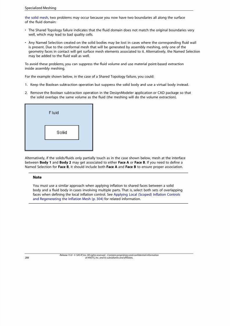
8/10/2019 ANSYS Meshing Users Guide
http://slidepdf.com/reader/full/ansys-meshing-users-guide 296/491
the solid mesh, two problems may occur because you now have two boundaries all along the surfaceof the fluid domain:
• The Shared Topology failure indicates that the fluid domain does not match the original boundaries verywell, which may lead to bad quality cells.
• Any Named Selection created on the solid bodies may be lost in cases where the corresponding fluid wall
is present. Due to the conformal mesh that will be generated by assembly meshing, only one of the
geometry faces in contact will get surface mesh elements associated to it. Alternatively, the Named Selectionmay be added to the fluid wall as well.
To avoid these problems, you can suppress the fluid volume and use material point-based extractioninside assembly meshing.
For the example shown below, in the case of a Shared Topology failure, you could:
1. Keep the Boolean subtraction operation but suppress the solid body and use a virtual body instead.
2. Remove the Boolean subtraction operation in the DesignModeler application or CAD package so thatthe solid overlaps the same volume as the fluid (the meshing will do the volume extraction).
Alternatively, if the solids/fluids only partially touch as in the case shown below, mesh at the interfacebetween Body 1 and Body 2 may get associated to either Face A or Face B. If you need to define aNamed Selection for Face B, it should include both Face A and Face B to ensure proper association.
Note
You must use a similar approach when applying inflation to shared faces between a solid
body and a fluid body in cases involving multiple parts. That is, select both sets of overlappingfaces when defining the local inflation control. See Applying Local (Scoped) Inflation Controlsand Regenerating the Inflation Mesh (p. 304) for related information.
Release 15.0 - © SAS IP, Inc. All rights reserved. - Contains proprietary and confidential informationof ANSYS, Inc. and its subsidiaries and affiliates.288
Specialized Meshing
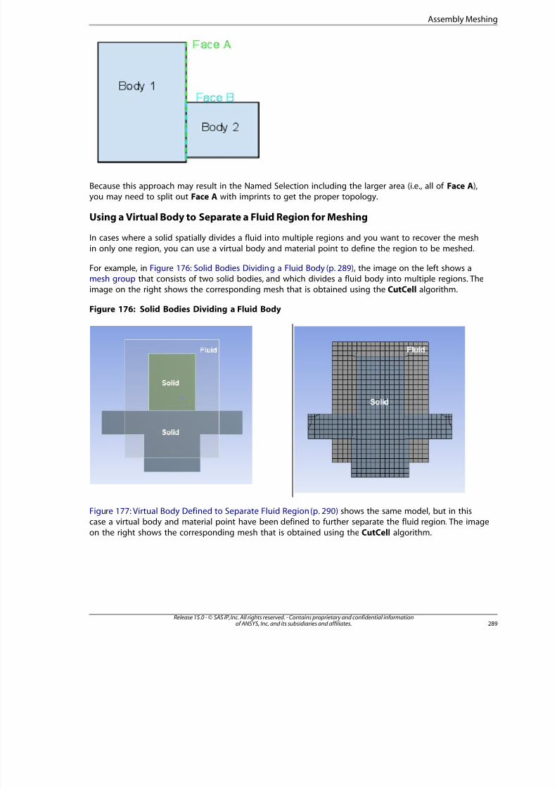
8/10/2019 ANSYS Meshing Users Guide
http://slidepdf.com/reader/full/ansys-meshing-users-guide 297/491
Because this approach may result in the Named Selection including the larger area (i.e., all of Face A),you may need to split out Face A with imprints to get the proper topology.
Using a Virtual Body to Separate a Fluid Region for Meshing
In cases where a solid spatially divides a fluid into multiple regions and you want to recover the mesh
in only one region, you can use a virtual body and material point to define the region to be meshed.
For example, in Figure 176: Solid Bodies Dividing a Fluid Body (p. 289), the image on the left shows amesh group that consists of two solid bodies, and which divides a fluid body into multiple regions. Theimage on the right shows the corresponding mesh that is obtained using the CutCell algorithm.
Figure 176: Solid Bodies Dividing a Fluid Body
Figure 177: Virtual Body Defined to Separate Fluid Region (p. 290) shows the same model, but in thiscase a virtual body and material point have been defined to further separate the fluid region. The image
on the right shows the corresponding mesh that is obtained using the CutCell algorithm.
289Release 15.0 - © SAS IP, Inc. All rights reserved. - Contains proprietary and confidential informationof ANSYS, Inc. and its subsidiaries and affiliates.
Assembly Meshing
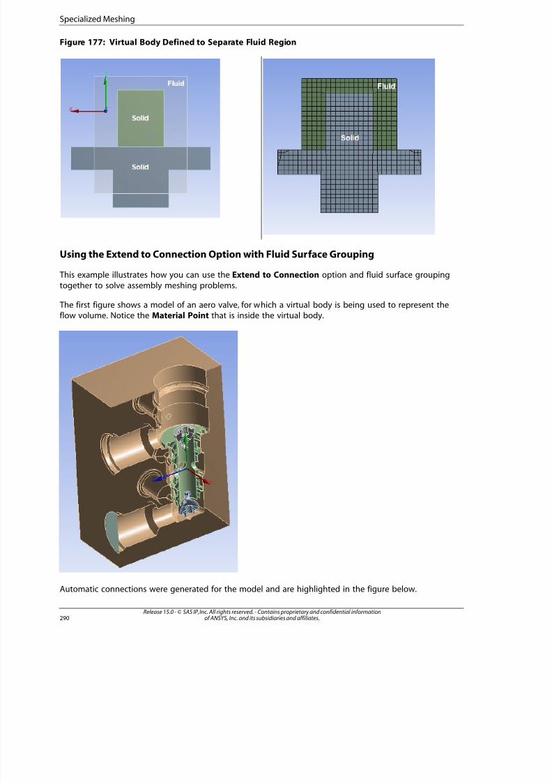
8/10/2019 ANSYS Meshing Users Guide
http://slidepdf.com/reader/full/ansys-meshing-users-guide 298/491
Figure 177: Virtual Body Defined to Separate Fluid Region
Using the Extend to Connection Option with Fluid Surface Grouping
This example illustrates how you can use the Extend to Connection option and fluid surface grouping
together to solve assembly meshing problems.
The first figure shows a model of an aero valve, for which a virtual body is being used to represent theflow volume. Notice the Material Point that is inside the virtual body.
Automatic connections were generated for the model and are highlighted in the figure below.
Release 15.0 - © SAS IP, Inc. All rights reserved. - Contains proprietary and confidential informationof ANSYS, Inc. and its subsidiaries and affiliates.290
Specialized Meshing
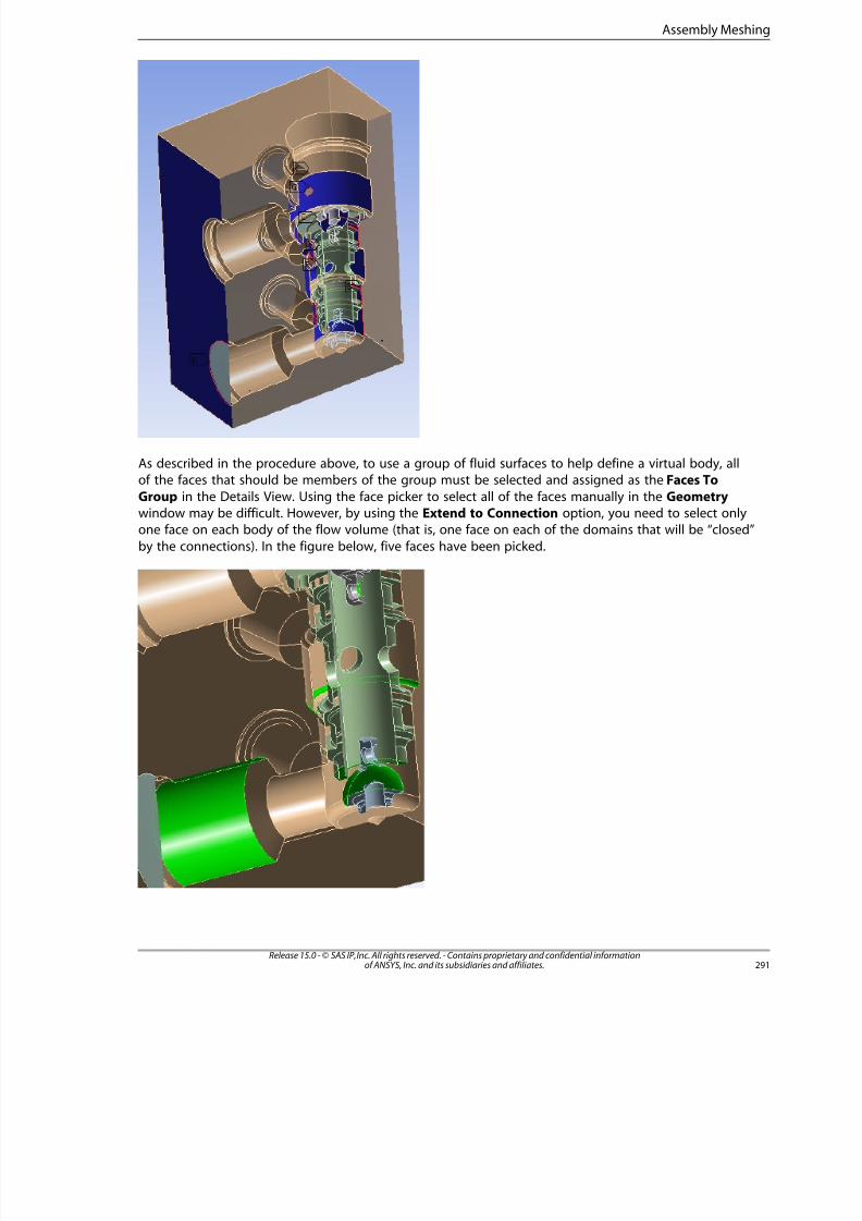
8/10/2019 ANSYS Meshing Users Guide
http://slidepdf.com/reader/full/ansys-meshing-users-guide 299/491
As described in the procedure above, to use a group of fluid surfaces to help define a virtual body, allof the faces that should be members of the group must be selected and assigned as the Faces To
Group in the Details View. Using the face picker to select all of the faces manually in the Geometrywindow may be difficult. However, by using the Extend to Connection option, you need to select onlyone face on each body of the flow volume (that is, one face on each of the domains that will be “closed”
by the connections). In the figure below, five faces have been picked.
29Release 15.0 - © SAS IP, Inc. All rights reserved. - Contains proprietary and confidential informationof ANSYS, Inc. and its subsidiaries and affiliates.
Assembly Meshing
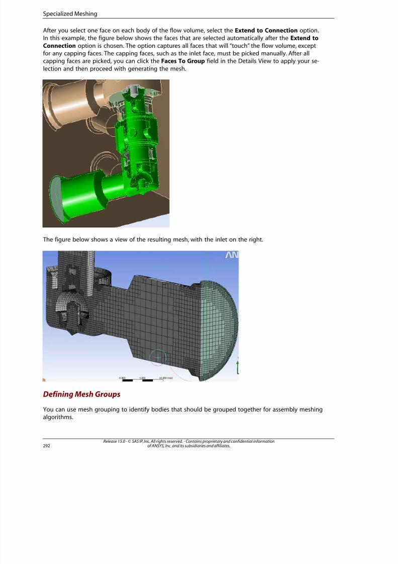
8/10/2019 ANSYS Meshing Users Guide
http://slidepdf.com/reader/full/ansys-meshing-users-guide 300/491
After you select one face on each body of the flow volume, select the Extend to Connection option.In this example, the figure below shows the faces that are selected automatically after the Extend to
Connection option is chosen. The option captures all faces that will “touch” the flow volume, exceptfor any capping faces. The capping faces, such as the inlet face, must be picked manually. After allcapping faces are picked, you can click the Faces To Group field in the Details View to apply your se-
lection and then proceed with generating the mesh.
The figure below shows a view of the resulting mesh, with the inlet on the right.
Defining Mesh Groups
You can use mesh grouping to identify bodies that should be grouped together for assembly meshingalgorithms.
Release 15.0 - © SAS IP, Inc. All rights reserved. - Contains proprietary and confidential informationof ANSYS, Inc. and its subsidiaries and affiliates.292
Specialized Meshing

8/10/2019 ANSYS Meshing Users Guide
http://slidepdf.com/reader/full/ansys-meshing-users-guide 301/491
Mesh Group objects appear in the Tree Outline under the Mesh object. The purpose of a Mesh Groupobject is to unite bodies that have the same properties and do not have gaps between them. For example
this approach may be useful if you decomposed a fluid volume into multiple volumes for hybridmeshing but now want to use the CutCell approach to mesh the same model. With CutCell, decomposedvolumes are no longer needed. Grouping tells the mesher to treat certain solid parts as one part. You
can define a mesh group to merge volumes, and the mesh generated on the combined parts (i.e., thegroup) will be associated with the mesh of the selected master body.
Note
Only solid (3D) bodies can be selected for grouping. Surface bodies cannot be selected.
Defining a Mesh Group
The steps for defining a mesh group are presented here.
1. To insert a Mesh Group object into the Tree, highlight the Mesh object (or its Mesh Grouping or MesGroup child object if any exist) and then do one of the following:
• Select Mesh Control> Mesh Group on the Mesh context toolbar.
• Click the right mouse button on the object you highlighted and select Insert> Mesh Group from thcontext menu.
These methods insert a Mesh Group object beneath the Mesh Grouping object. The Mesh
Grouping object is inserted automatically when the first Mesh Group object is inserted.
2. To define and make adjustments to an individual group, click a Mesh Group object and use the followcontrols. These controls appear in the Details View of the Mesh Group object.
• Bodies To Group: In the Geometry window, select the bodies that should be members of the group
– All bodies within a group, including the Master Body, should be of the same type (i.e., Fluid orSolid, as defined by the Fluid/Solid material property). Otherwise, unexpected results may occur.
– Surface bodies cannot be selected for grouping.
• Master Body: In the Geometry window, select the body that should act as the master of the group. The master body is the body to which all mesh of the group members will be associated. By default,the first body that is selected for Bodies To Group is the Master Body.
• Priority: Determines which group will claim cells in cases where groups overlap. The priority is initialbased on the rule: the smaller the volume, the higher the priority.
• Suppressed: Toggles suppression of the selected group. The default is No. If set to Yes, the group
will be suppressed.
Setting Global Assembly Meshing Options
The next step in the assembly meshing workflow is to define global assembly meshing options:
1. Select the appropriate option for Feature Capture (p. 98).
2. Select the appropriate option for Tessellation Refinement (p. 98).
293Release 15.0 - © SAS IP, Inc. All rights reserved. - Contains proprietary and confidential informationof ANSYS, Inc. and its subsidiaries and affiliates.
Assembly Meshing
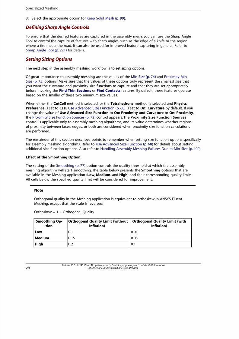
8/10/2019 ANSYS Meshing Users Guide
http://slidepdf.com/reader/full/ansys-meshing-users-guide 302/491
3. Select the appropriate option for Keep Solid Mesh (p. 99).
Defining Sharp Angle Controls
To ensure that the desired features are captured in the assembly mesh, you can use the Sharp Angle
Tool to control the capture of features with sharp angles, such as the edge of a knife or the regionwhere a tire meets the road. It can also be used for improved feature capturing in general. Refer toSharp Angle Tool (p. 221) for details.
Setting Sizing Options
The next step in the assembly meshing workflow is to set sizing options.
Of great importance to assembly meshing are the values of the Min Size (p. 74) and Proximity MinSize (p. 75) options. Make sure that the values of these options truly represent the smallest size thatyou want the curvature and proximity size functions to capture and that they are set appropriately
before invoking the Find Thin Sections or Find Contacts features. By default, these features operatebased on the smaller of these two minimum size values.
When either the CutCell method is selected, or the Tetrahedrons method is selected and PhysicsPreference is set to CFD, Use Advanced Size Function (p. 68) is set to On: Curvature by default. If you
change the value of Use Advanced Size Function to On: Proximity and Curvature or On: Proximity,the Proximity Size Function Sources (p. 72) control appears. The Proximity Size Function Sourcescontrol is applicable only to assembly meshing algorithms, and its value determines whether regions
of proximity between faces, edges, or both are considered when proximity size function calculationsare performed.
The remainder of this section describes points to remember when setting size function options specificallyfor assembly meshing algorithms. Refer to Use Advanced Size Function (p. 68) for details about setting
additional size function options. Also refer to Handling Assembly Meshing Failures Due to Min Size (p. 400).
Effect of the Smoothing Option:
The setting of the Smoothing (p. 77) option controls the quality threshold at which the assembly
meshing algorithm will start smoothing. The table below presents the Smoothing options that areavailable in the Meshing application (Low, Medium, and High) and their corresponding quality limits.All cells below the specified quality limit will be considered for improvement.
Note
Orthogonal quality in the Meshing application is equivalent to orthoskew in ANSYS FluentMeshing, except that the scale is reversed:
Orthoskew = 1 – Orthogonal Quality
Orthogonal Quality Limit (withInflation)
Orthogonal Quality Limit (withoutInflation)
Smoothing Op-tion
0.010.1Low
0.050.15Medium
0.10.2High
Release 15.0 - © SAS IP, Inc. All rights reserved. - Contains proprietary and confidential informationof ANSYS, Inc. and its subsidiaries and affiliates.294
Specialized Meshing

8/10/2019 ANSYS Meshing Users Guide
http://slidepdf.com/reader/full/ansys-meshing-users-guide 303/491
Refer to Orthogonal Quality (p. 138) for more information.
Note
When the Tetrahedrons algorithm is being used and Smoothing is set to Low, only minimal
surface mesh improvement occurs, which provides a faster turnaround for large cases having
many faces. Thus, you can choose between higher quality mesh vs. faster turnaround.
Rules for Computing Min Size and Max Size:
Assembly meshing algorithms use the following rules for computing Min Size and Max Size values,
where the value of Min Size is the smaller of the two minimum size values (i.e., Min Size or ProximityMin Size). In general, the Max Size value is computed based on the Min Size value, such that a 2^nratio is maintained:
1. Default Max Size = Default Min Size * 128.
2. The ratio between Min Size and Max Size can be any one of the powers of two from 0 to 13 (shown in
the table below). Thus, 14 levels of difference between Min Size and Max Size are allowed:
2^7 = 1282^0 = 1
2^8 = 2562^1 = 2
2^9 = 5122^2 = 4
2^10 = 10242^3 = 8
2^11 = 20482^4 = 16
2^12 = 40962^5 = 32
2^13 = 81922^6 = 64
Note
The value of Max Size cannot be greater than (2^13 * Min Size). If the value you set forMax Size is too high, Max Size is set to its maximum limit (2^13 * Min Size) automatically.
3. Max Size may be converted to the power of two that is nearest to the intended value of Max Size, whethe intended value of Max Size is either the default value or the user input value of Max Size.
Consider this example, which shows the Min Size and Max Size values at each step in the given se-
quence:
1. Select an assembly meshing algorithm. Default Min Size = 5, so default Max Size = 5 * 128 = 640.
Min Size, Max Size = Default(5.0), Default(640.0)
2. If you set Min Size to any one of {0.0625, 0.125, 0.25, 0.5, 1, 2, 4, ... 512, ... 2^n}, then Max Size = 512(not default). For example, if you set Min Size = 1, (Min Size, Max Size) = (1, 512).
3. Set Max Size = 40,000, Max Size = 8192 based on the maximum limit rule described above.
Min Size, Max Size = 1, 8192
295Release 15.0 - © SAS IP, Inc. All rights reserved. - Contains proprietary and confidential informationof ANSYS, Inc. and its subsidiaries and affiliates.
Assembly Meshing
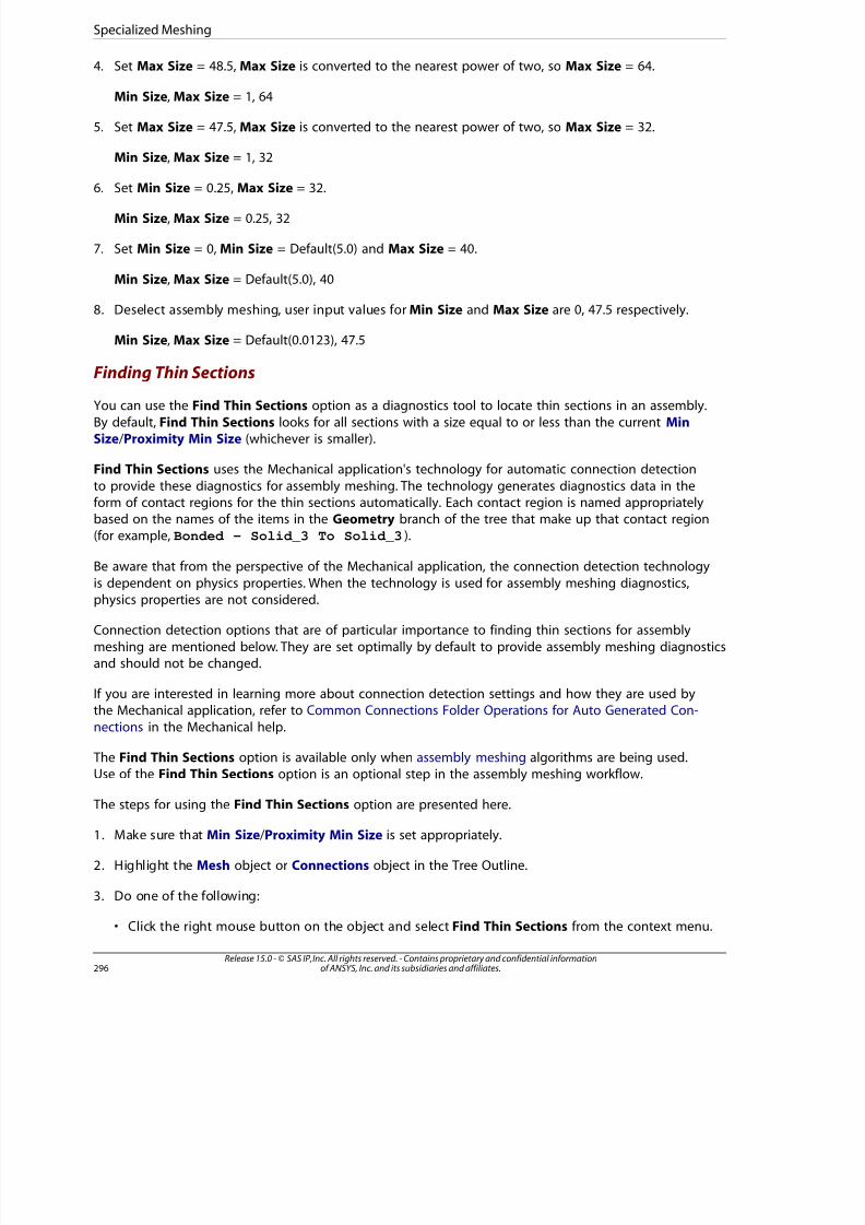
8/10/2019 ANSYS Meshing Users Guide
http://slidepdf.com/reader/full/ansys-meshing-users-guide 304/491
4. Set Max Size = 48.5, Max Size is converted to the nearest power of two, so Max Size = 64.
Min Size, Max Size = 1, 64
5. Set Max Size = 47.5, Max Size is converted to the nearest power of two, so Max Size = 32.
Min Size, Max Size = 1, 32
6. Set Min Size = 0.25, Max Size = 32.
Min Size, Max Size = 0.25, 32
7. Set Min Size = 0, Min Size = Default(5.0) and Max Size = 40.
Min Size, Max Size = Default(5.0), 40
8. Deselect assembly meshing, user input values for Min Size and Max Size are 0, 47.5 respectively.
Min Size, Max Size = Default(0.0123), 47.5
Finding Thin Sections
You can use the Find Thin Sections option as a diagnostics tool to locate thin sections in an assembly.
By default, Find Thin Sections looks for all sections with a size equal to or less than the current MinSize /Proximity Min Size (whichever is smaller).
Find Thin Sections uses the Mechanical application's technology for automatic connection detection
to provide these diagnostics for assembly meshing. The technology generates diagnostics data in theform of contact regions for the thin sections automatically. Each contact region is named appropriatelybased on the names of the items in the Geometry branch of the tree that make up that contact region(for example, Bonded - Solid_3 To Solid_3).
Be aware that from the perspective of the Mechanical application, the connection detection technology
is dependent on physics properties. When the technology is used for assembly meshing diagnostics,physics properties are not considered.
Connection detection options that are of particular importance to finding thin sections for assembly
meshing are mentioned below. They are set optimally by default to provide assembly meshing diagnosticsand should not be changed.
If you are interested in learning more about connection detection settings and how they are used bythe Mechanical application, refer to Common Connections Folder Operations for Auto Generated Con-
nections in the Mechanical help.
The Find Thin Sections option is available only when assembly meshing algorithms are being used.
Use of the Find Thin Sections option is an optional step in the assembly meshing workflow.
The steps for using the Find Thin Sections option are presented here.
1. Make sure that Min Size /Proximity Min Size is set appropriately.
2. Highlight the Mesh object or Connections object in the Tree Outline.
3. Do one of the following:
• Click the right mouse button on the object and select Find Thin Sections from the context menu.
Release 15.0 - © SAS IP, Inc. All rights reserved. - Contains proprietary and confidential informationof ANSYS, Inc. and its subsidiaries and affiliates.296
Specialized Meshing
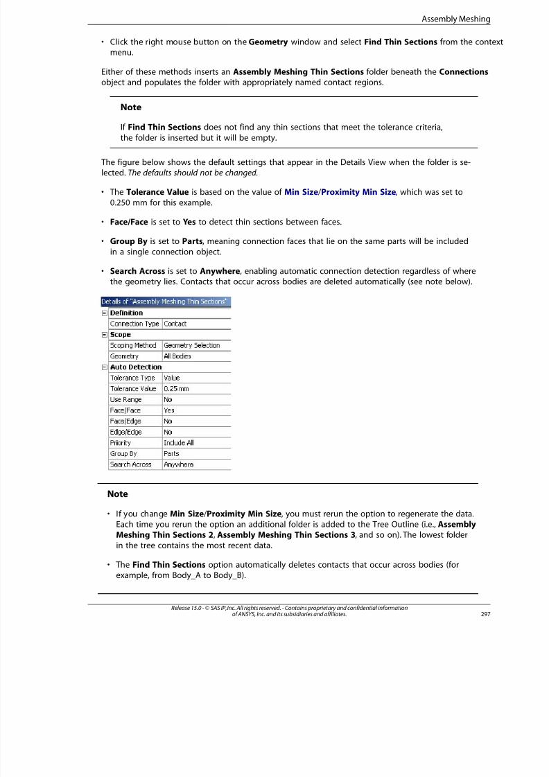
8/10/2019 ANSYS Meshing Users Guide
http://slidepdf.com/reader/full/ansys-meshing-users-guide 305/491
• Click the right mouse button on the Geometry window and select Find Thin Sections from the conmenu.
Either of these methods inserts an Assembly Meshing Thin Sections folder beneath the Connectionsobject and populates the folder with appropriately named contact regions.
Note
If Find Thin Sections does not find any thin sections that meet the tolerance criteria,
the folder is inserted but it will be empty.
The figure below shows the default settings that appear in the Details View when the folder is se-lected. The defaults should not be changed.
• The Tolerance Value is based on the value of Min Size /Proximity Min Size, which was set to
0.250 mm for this example.
• Face/Face is set to Yes to detect thin sections between faces.
• Group By is set to Parts, meaning connection faces that lie on the same parts will be includedin a single connection object.
• Search Across is set to Anywhere, enabling automatic connection detection regardless of wherethe geometry lies. Contacts that occur across bodies are deleted automatically (see note below).
Note
• If you change Min Size /Proximity Min Size, you must rerun the option to regenerate the data.Each time you rerun the option an additional folder is added to the Tree Outline (i.e., AssemblyMeshing Thin Sections 2, Assembly Meshing Thin Sections 3, and so on). The lowest folder
in the tree contains the most recent data.
• The Find Thin Sections option automatically deletes contacts that occur across bodies (forexample, from Body_A to Body_B).
297Release 15.0 - © SAS IP, Inc. All rights reserved. - Contains proprietary and confidential informationof ANSYS, Inc. and its subsidiaries and affiliates.
Assembly Meshing
8/10/2019 ANSYS Meshing Users Guide
http://slidepdf.com/reader/full/ansys-meshing-users-guide 306/491
Finding Contacts
You can use the Find Contacts option as a diagnostics tool to locate contacts in an assembly. By default,Find Contacts detects face-edge contacts using a tolerance based on the current Min Size /Proximity
Min Size (whichever is smaller) as follows:
• Contacts between 10% of Min Size /Proximity Min Size and 0
The search for contacts passes feature information down to the meshing algorithm to ensure that desiredfeatures are preserved. In addition to the edges that are determined to be feature edges based on theassembly meshing angle criterion, edges referenced in contact regions are also considered as featureedges in assembly meshing. Find Contacts is particularly useful for assemblies in which fillets of bodiesare adjacent to other bodies, forming a sharp angle, as it will preserve the edges of these fillets inde-
pendent of the feature angle settings.
Find Contacts uses the Mechanical application's technology for automatic connection detection toprovide these diagnostics for assembly meshing. The technology generates diagnostics data in the form
of contact regions for the contacts automatically. Each contact region is named appropriately based onthe names of the items in the Geometry branch of the tree that make up that contact region (for ex-ample, Bonded - Solid_2 To Solid_4).
Be aware that from the perspective of the Mechanical application, the connection detection technologyis dependent on physics properties. When the technology is used for assembly meshing diagnostics,
physics properties are not considered.
Connection detection options that are of particular importance to finding contacts for assembly meshingare mentioned below. They are set optimally by default to provide assembly meshing diagnostics andshould not be changed.
If you are interested in learning more about connection detection settings and how they are used bythe Mechanical application, refer to Common Connections Folder Operations for Auto Generated Con-nections in the Mechanical help.
The Find Contacts option is available only when assembly meshing algorithms are being used.
The steps for using the Find Contacts option are presented here.
1. Make sure that Min Size /Proximity Min Size is set appropriately.
2. Highlight the Mesh object or Connections object in the Tree Outline.
3. Do one of the following:
• Click the right mouse button on the object and select Find Contacts from the context menu.
• Click the right mouse button on the Geometry window and select Find Contacts from the contextmenu.
Release 15.0 - © SAS IP, Inc. All rights reserved. - Contains proprietary and confidential informationof ANSYS, Inc. and its subsidiaries and affiliates.298
Specialized Meshing
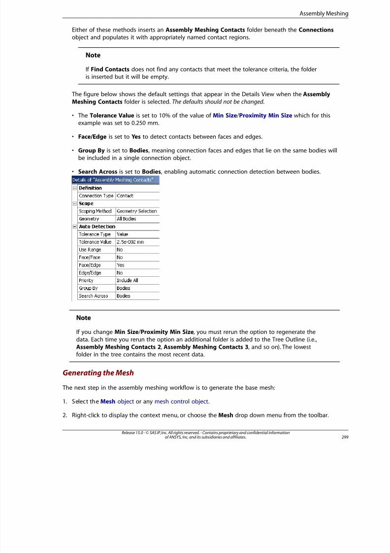
8/10/2019 ANSYS Meshing Users Guide
http://slidepdf.com/reader/full/ansys-meshing-users-guide 307/491
Either of these methods inserts an Assembly Meshing Contacts folder beneath the Connectionsobject and populates it with appropriately named contact regions.
Note
If Find Contacts does not find any contacts that meet the tolerance criteria, the folderis inserted but it will be empty.
The figure below shows the default settings that appear in the Details View when the Assembly
Meshing Contacts folder is selected. The defaults should not be changed.
• The Tolerance Value is set to 10% of the value of Min Size /Proximity Min Size which for thisexample was set to 0.250 mm.
• Face/Edge is set to Yes to detect contacts between faces and edges.
• Group By is set to Bodies, meaning connection faces and edges that lie on the same bodies willbe included in a single connection object.
• Search Across is set to Bodies, enabling automatic connection detection between bodies.
Note
If you change Min Size /Proximity Min Size, you must rerun the option to regenerate the
data. Each time you rerun the option an additional folder is added to the Tree Outline (i.e.,
Assembly Meshing Contacts 2, Assembly Meshing Contacts 3, and so on). The lowestfolder in the tree contains the most recent data.
Generating the Mesh
The next step in the assembly meshing workflow is to generate the base mesh:
1. Select the Mesh object or any mesh control object.
2. Right-click to display the context menu, or choose the Mesh drop down menu from the toolbar.
299Release 15.0 - © SAS IP, Inc. All rights reserved. - Contains proprietary and confidential informationof ANSYS, Inc. and its subsidiaries and affiliates.
Assembly Meshing
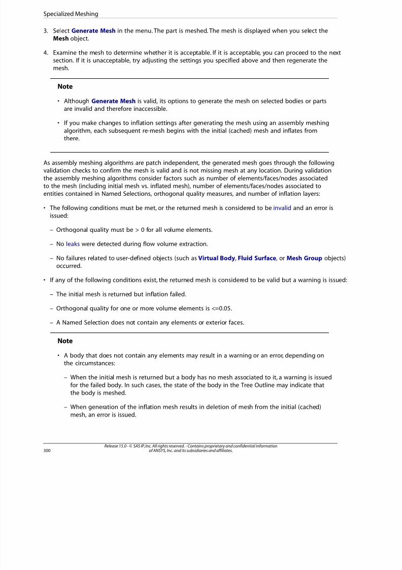
8/10/2019 ANSYS Meshing Users Guide
http://slidepdf.com/reader/full/ansys-meshing-users-guide 308/491
3. Select Generate Mesh in the menu. The part is meshed. The mesh is displayed when you select theMesh object.
4. Examine the mesh to determine whether it is acceptable. If it is acceptable, you can proceed to the nextsection. If it is unacceptable, try adjusting the settings you specified above and then regenerate themesh.
Note• Although Generate Mesh is valid, its options to generate the mesh on selected bodies or parts
are invalid and therefore inaccessible.
• If you make changes to inflation settings after generating the mesh using an assembly meshing
algorithm, each subsequent re-mesh begins with the initial (cached) mesh and inflates fromthere.
As assembly meshing algorithms are patch independent, the generated mesh goes through the followingvalidation checks to confirm the mesh is valid and is not missing mesh at any location. During validation
the assembly meshing algorithms consider factors such as number of elements/faces/nodes associatedto the mesh (including initial mesh vs. inflated mesh), number of elements/faces/nodes associated toentities contained in Named Selections, orthogonal quality measures, and number of inflation layers:
• The following conditions must be met, or the returned mesh is considered to be invalid and an error isissued:
– Orthogonal quality must be > 0 for all volume elements.
– No leaks were detected during flow volume extraction.
– No failures related to user-defined objects (such as Virtual Body, Fluid Surface, or Mesh Group objects)
occurred.
• If any of the following conditions exist, the returned mesh is considered to be valid but a warning is issued:
– The initial mesh is returned but inflation failed.
– Orthogonal quality for one or more volume elements is <=0.05.
– A Named Selection does not contain any elements or exterior faces.
Note
• A body that does not contain any elements may result in a warning or an error, depending onthe circumstances:
– When the initial mesh is returned but a body has no mesh associated to it, a warning is issued
for the failed body. In such cases, the state of the body in the Tree Outline may indicate thatthe body is meshed.
– When generation of the inflation mesh results in deletion of mesh from the initial (cached)
mesh, an error is issued.
Release 15.0 - © SAS IP, Inc. All rights reserved. - Contains proprietary and confidential informationof ANSYS, Inc. and its subsidiaries and affiliates.300
Specialized Meshing
8/10/2019 ANSYS Meshing Users Guide
http://slidepdf.com/reader/full/ansys-meshing-users-guide 309/491
• The assembly meshing algorithms may not be able to support cases where surfaces form across. For example, the four bodies in the image below form a cross as depicted by the thick
lines. In such cases, the feature recovery/surface recovery along the center line (shown as thecenter point in the 2D image below) may be poor.
• Using a different facet quality in the DesignModeler application could have an impact on the
performance and quality of assembly meshing. Increasing the facet quality could improve featurecapturing, reduce leakage, and improve quality (refer to Avoiding Bad Feature Capturing inAssembly Meshing (p. 400)), but at the same time it could increase the assembly meshing time,
particularly for tetrahedron.
• Refer to "Meshing: Troubleshooting" (p. 391) for additional tips and strategies for handlingproblems that may occur during assembly meshing.
Applying Contact Sizing
When used with assembly meshing, contact sizing provides a method for closing leaks discovered
during meshing. Typically, leakage occurs if any contact is larger than 1/10 of the local minimum size.If a leak is discovered during meshing and the gap is up to 1/3 of the local mesh size, you can closethe gap at the location of contact by using a two-step process. First, scope a new contact to the existingFind Contacts list by picking all of the faces on one side and all of the faces (or edges) on the other
side of the leak. Second, scope a contact sizing control to this new contact.
For assembly meshing, the default Element Size used by contact sizing controls is minimum_size/5,where minimum_size is the value of Min Size or Proximity Min Size, whichever is smaller. This Element
Size is appropriate for the vast majority of cases. However, you may need to adjust the value of ElementSize in these situations:
• If hard sizing that is smaller than Min Size /Proximity Min Size is applied in the vicinity of the contactregion, you may need to reduce the Element Size used by contact.
30Release 15.0 - © SAS IP, Inc. All rights reserved. - Contains proprietary and confidential informationof ANSYS, Inc. and its subsidiaries and affiliates.
Assembly Meshing

8/10/2019 ANSYS Meshing Users Guide
http://slidepdf.com/reader/full/ansys-meshing-users-guide 310/491
• If local sizing that is significantly larger than Min Size /Proximity Min Size is applied in the vicinity of thecontact region, you may need to increase the Element Size used by contact.
Note
• Each face-edge contact region in a contact sizing control consists of one or more faces andone or more edges. That is, in some cases a contact region may consist of one face to one edge
in contact, while in others it may consist of many faces to many edges.
• Use care in specifying Element Size for contact sizing. A value that is too large may lead toinaccurate geometry, while a value that is too small may fail to close the leak. A good guidelineis to specify an Element Size that is 1/5 of the local element size.
• In some cases the gap at the location of contact is closed but the mesh in that location willnot be well resolved. This occurs because there are no features to be captured at the locationof the gap, which in turn causes the edges to become jagged.
You can apply contact sizing using either of the following methods:
Method 1
1. In the Tree Outline, select the Mesh object or any mesh control object.
2. Do one of the following:
a. Choose Contact Sizing from the Mesh Control drop-down menu.
b. Right-click on the selected object and select Insert> Contact Sizing from the context menu.
A new Contact Sizing control is added to the Tree Outline.
3. In the Details View, select a specific Contact Region to scope it to the sizing control.
4. Enter a value for Element Size. By default, Element Size is set equal to the value of minimum_size/5.
Method 2
1. In the Tree Outline, drag a contact region from the Assembly Meshing Contacts folder onto the Meshobject.
A new Contact Sizing control is added to the Tree Outline.
2. In the Tree Outline, highlight the new Contact Sizing control.
3. Enter a value for Element Size. By default, Element Size is set equal to the value of minimum_size/5.
Note
• The Element Size option for Type specifies an absolute size for the contact sizing. The Relev-
ance option for Type, which is sometimes used to specify a relative size in contact sizing con-trols, is not supported for assembly meshing algorithms.
Release 15.0 - © SAS IP, Inc. All rights reserved. - Contains proprietary and confidential informationof ANSYS, Inc. and its subsidiaries and affiliates.302
Specialized Meshing
8/10/2019 ANSYS Meshing Users Guide
http://slidepdf.com/reader/full/ansys-meshing-users-guide 311/491
• If contact sizing is applied to entities on a body that is scoped to a body of influence, thecontact sizing is ignored.
• If you apply contact sizing and a sharp angle control to the same face, the sharp angle featuresmay not be captured accurately.
Setting Global Inflation Controls
After you determine the base mesh is acceptable, the next step in the assembly meshing workflow isto set global inflation controls:
Note
When an assembly meshing algorithm is being used, a mixture of global (automatic ProgramControlled) and local (scoped) inflation is not supported . See Selecting an Assembly MeshMethod (p. 279) for details about behaviors resulting from this restriction and guidelines for
using global vs. local inflation.
1. Set Use Automatic Inflation (p. 80) to Program Controlled (p. 81).
The All Faces in Chosen Named Selection option is not supported for assembly meshing algorithms.If this option is specified and you select an assembly meshing algorithm, the option will be changed
automatically to Program Controlled and a warning will be issued.
2. Set additional global inflation controls as desired. Refer to Inflation Group (p. 78) for descriptions.
Note
• The Fluid/Solid material property for virtual bodies is always set to Fluid (read-only). With
Program Controlled inflation, faces on real solid bodies will inflate into the virtual bodies. TheFluid/Solid designation on real bodies will be respected (that is, faces on real fluid bodies willinflate into the fluid region, but the solid region will not be inflated).
• Attempting to grow thicker prism layers in areas where the aspect ratio of the base to the
prism cap is very large may result in an invalid mesh. In such cases (e.g., external flow problems),it is recommended to use aspect ratio based growth to avoid problems with invalid meshes.
Generating the Inflation Mesh
The next step in the assembly meshing workflow is to generate the inflation mesh:
1. Select the Mesh object or any mesh control object.
2. Right-click to display the context menu, or choose the Mesh drop down menu from the toolbar.
3. Select Generate Mesh in the menu. The inflation mesh is generated and is displayed when you selectthe Mesh object.
4. Examine the inflation mesh, which was obtained using automatic Program Controlled inflation. If it isacceptable, you can proceed directly to Exporting the Mesh (p. 306). If it is unacceptable, you can either
303Release 15.0 - © SAS IP, Inc. All rights reserved. - Contains proprietary and confidential informationof ANSYS, Inc. and its subsidiaries and affiliates.
Assembly Meshing
8/10/2019 ANSYS Meshing Users Guide
http://slidepdf.com/reader/full/ansys-meshing-users-guide 312/491
adjust the global inflation controls described above or proceed to the next section to set local inflationcontrols, and then regenerate the inflation mesh.
Note
• For assembly meshing algorithms, inflation is a post process for the mesher after it has createdthe hexahedron or tetrahedron elements. A benefit of this approach is that the hexahedral/tet-
rahedral mesh does not have to be generated each time inflation options are changed. Youcan add/delete/modify/suppress your inflation settings, and the meshing process will beginwith the initial (cached) mesh and inflate from there. This is important in case you need tomake adjustments to obtain the desired results.
• In cases in which Smoothing (p. 77) is set to High and CutCell meshing is being used, addi-
tional smoothing of inflation layers occurs. This may slow down the prism generation process.
Applying Local (Scoped) Inflation Controls and Regenerating the Inflation Mesh
If the inflation mesh that was generated using global (automatic Program Controlled) inflation is ac-
ceptable, you can proceed directly to Exporting the Mesh (p. 306). If it is unacceptable, you can applylocal inflation controls to try to improve the mesh.
Note
• When an assembly meshing algorithm is being used, a mixture of global and local inflation isnot supported . See Selecting an Assembly Mesh Method (p. 279) for details about behaviorsresulting from this restriction and guidelines for using global vs. local inflation.
• If mesh groups are present, you must scope local inflation controls to either the master bodyor to all bodies in the mesh group. Otherwise, mesh generation fails. Alternatively, you can set
the Fluid/Solid material property settings for the bodies to Fluid and use global (ProgramControlled) inflation instead. Refer to Program Controlled (p. 81) for more information.
To add boundary layers to a face for assembly meshing:
1. In the global inflation controls, set Use Automatic Inflation (p. 80) to None (p. 80). Otherwise, you willnot be able to insert local inflation.
2. Optionally, select the desired bodies in the Geometry window. These are the bodies that you want toscope inflation to.
3. Use either of these methods to insert the inflation control:
• Click Mesh Control on the toolbar and choose Inflation from the menu.
• Right-click in the Geometry window and choose Insert > Inflation from the menu.
4. If you selected the bodies in step 2, go directly to step 5. If not, use either of these methods to scope
inflation to the desired bodies:
• In the Details View, set Scoping Method to Geometry Selection, pick the bodies in the Geometrywindow, and click the Geometry field in the Details View to Apply.
Release 15.0 - © SAS IP, Inc. All rights reserved. - Contains proprietary and confidential informationof ANSYS, Inc. and its subsidiaries and affiliates.304
Specialized Meshing
8/10/2019 ANSYS Meshing Users Guide
http://slidepdf.com/reader/full/ansys-meshing-users-guide 313/491
• In the Details View, set Scoping Method to Named Selection, and select a Named Selection from thNamed Selection drop-down.
5. Change the value of the Suppressed control if desired.
By default, the value of Suppressed is No. If you change the value to Yes, this inflation control hasno effect on the mesh. In addition, an Active control with a read-only setting of No, Suppressed
appears under the Suppressed control when Suppressed is set to Yes.
6. Use either of these methods to specify the inflation boundaries (i.e., select the faces that you want theinflation layers to grow away from):
• In the Details View, set Boundary Scoping Method to Geometry Selection, pick the faces in theGeometry window, and click the Boundary field in the Details View to Apply.
• In the Details View, set Boundary Scoping Method to Named Selections, select a Named Selection
from the Boundary drop-down, and press Enter.
Note
– To select multiple Named Selections to be used as inflation boundaries, press and holdthe CTRL key while selecting the Named Selections from the Boundary drop-down, andthen press Enter.
– If none of the predefined Named Selections include the correct topology to be used asan inflation boundary, no Named Selections will be available in the drop-down. For as-sembly meshing algorithms, the correct topology is always a face because 2D inflation
is not supported (see notes below). If any 2D inflation controls are defined prior to selec-tion of an assembly meshing algorithm, they are suppressed when an assembly meshingalgorithm is selected.
– For assembly meshing algorithms only, the scoped body and the face that you select to
be the inflation boundary do not have to be on the same part. In other words, the facedoes not have to be attached to the body. Such controls are invalid for part/body levelmeshing, and will be flagged as invalid if any have been defined and you subsequently
deselect assembly meshing. The scoped body will be retained but you will have to selecta new inflation boundary.
– To apply inflation to shared faces between a solid body and a fluid body in cases involvingmultiple parts, you must select both sets of overlapping faces when defining the local
inflation control.
7. Specify additional inflation options, as desired, in the Details View. For descriptions of additional optionrefer to Inflation Group (p. 78).
8. Select the Mesh object or any mesh control object.
9. Right-click to display the context menu, or choose the Mesh drop down menu from the toolbar.
10. Select Generate Mesh in the menu. The inflation layers are regenerated, and the mesh is displayed wh
you select the Mesh object.
305Release 15.0 - © SAS IP, Inc. All rights reserved. - Contains proprietary and confidential informationof ANSYS, Inc. and its subsidiaries and affiliates.
Assembly Meshing
8/10/2019 ANSYS Meshing Users Guide
http://slidepdf.com/reader/full/ansys-meshing-users-guide 314/491
11. Continue making adjustments and experimenting with automatic Program Controlled inflation vs. localinflation until your results are satisfactory.
Note
• For inflation on virtual bodies, you must specify automatic Program Controlled inflation. Youcannot specify local controls to inflate virtual bodies.
• Assembly meshing algorithms do not support 2D inflation (i.e., inflation scoped to faces with
edges selected as boundaries).
• Assembly meshing algorithms do not support inflation on both sides of a face zone. If youapply inflation to a face zone that is shared by two cell zones of type fluid, the desired inflation
will not occur.
• Inflation on both sides of a baffle is supported for the Tetrahedrons algorithm only. Refer tothe discussion of inflation controls in Selecting an Assembly Mesh Method (p. 279) for moreinformation.
• If multiple inflation controls are defined and different numbers of layers are defined in them,the smallest defined number of layers will be respected for assembly meshing algorithms.
• If multiple inflation controls are defined, each with different values for Aspect Ratio
(Base/Height) (p. 86), the last value is the one that will be taken (i.e., the value specified forthe inflation control that appears lowest in the Tree Outline is honored) and will be used forall inflation controls for which Inflation Option (p. 83) is set to Last Aspect Ratio.
Exporting the Mesh
After you determine the inflation mesh is acceptable, the mesh is ready for export.
Points to remember when exporting an assembly mesh:
• Names of parts, bodies, and Named Selections should be limited to 64 characters.
• If you encounter a problem when using assembly meshing algorithms in the Meshing application,
you can export the faceted geometry to TGrid where you can display, interrogate, and repair the fa-ceted data.
• When a CutCell mesh is exported from the Meshing application to ANSYS Fluent, elements that are
connected to parent faces are exported in polyhedral format, while all others retain their type. Notethat this behavior is only true for CutCell; the Tetrahedrons algorithm uses only traditional element
types.
• When the mesh is exported to ANSYS Fluent, a cell zone type of either FLUID or SOLID is assigned to
each body based on its material properties. Refer to Fluent Mesh Export (p. 24) for details.
• Due to the 3D nature of the underlying meshing approach, mesh is not re-associated to any NamedSelection applied on vertices or edges. Hence, these Named Selections are not transferred to ANSYS
Fluent.
• When assembly meshing algorithms are used, mesh is associated to surface bodies in the Meshingapplication. The association is required in the Meshing application to ensure proper handling of the
Release 15.0 - © SAS IP, Inc. All rights reserved. - Contains proprietary and confidential informationof ANSYS, Inc. and its subsidiaries and affiliates.306
Specialized Meshing
8/10/2019 ANSYS Meshing Users Guide
http://slidepdf.com/reader/full/ansys-meshing-users-guide 315/491
mesh topology during internal processes. This requirement means that if your model contains surfacebodies, the element count reported in the Meshing application will differ from the cell count reported
in ANSYS Fluent for the same case.
• You cannot use assembly meshing in the Meshing application if you need to maintain the originalboundaries of overlapping surfaces and plan to use a non-conformal mesh interface in ANSYS Fluent.
If non-conformal mesh is needed, for example for sliding mesh problems, another mesh methodneeds to be used.
• Refer to Defining Virtual Bodies (p. 283) for information about export of virtual bodies to ANSYS Fluent.
Selective Meshing
Using selective meshing, you can selectively pick bodies and mesh them incrementally. After meshinga body, you can mesh the entire part or assembly or continue meshing individual bodies. To generate
the rest of the mesh in the model, use the Generate Mesh feature.
The following mesh methods are supported:
• For solid meshing:
– Patch Conforming Tetrahedron
– Patch Independent Tetrahedron
– MultiZone
– Sweep
– Hex Dominant
• For surface meshing:
– Quad Dominant
– All Triangles
– MultiZone Quad/Tri
Remember the following information when using selective meshing:
• Selective meshing is enabled by default. You can use the Allow Selective Meshing option to disable it.See Disabling Selective Meshing (p. 310) for information about Meshing application behaviors when sele
meshing is disabled.
• Selective meshing is not persistent for a geometry update or re-mesh operation. However, you can usethe Mesh worksheet to create a selective meshing history so that your meshing steps can be repeated ithe desired sequence. Otherwise, you must manually re-mesh bodies in the desired sequence. Refer to
Using the Mesh Worksheet to Create a Selective Meshing History (p. 311) for details.
• When using the Preview Surface Mesh, Preview Source and Target Mesh, or Preview Inflation featureduring selective meshing, the previewed mesh will be discarded when you perform a subsequent previe
or full mesh operation. The previewed mesh will not be used to seed the subsequent mesh operation.
307Release 15.0 - © SAS IP, Inc. All rights reserved. - Contains proprietary and confidential informationof ANSYS, Inc. and its subsidiaries and affiliates.
Selective Meshing

8/10/2019 ANSYS Meshing Users Guide
http://slidepdf.com/reader/full/ansys-meshing-users-guide 316/491
• After meshing, the meshed status icon appears in the Tree Outline for a meshed body within the Geometryfolder, or for a multibody part whose child bodies are all meshed. If you make changes after meshing that
invalidate the mesh for an individual body (such as adding sizing to the body), you will need to re-meshthat body only.
• In a multibody part, if any child bodies have been meshed and refined, another child body is unmeshed,
and you subsequently mesh the unmeshed body, the mesh state of all refined bodies in the part will beinvalidated and re-meshed during mesh generation. Similarly, if one body is unmeshed and refinement
is needed on another, generating the mesh will result in meshing and refinement of the entire part. Inaddition to cases involving refinement, this behavior applies in cases where post inflation is used.
• When meshing a body that is part of a symmetry object, match control, or pre pinch control, all bodiesthat the control is applied to need to be meshed at the same time. Also, if a body that is part of a symmetryobject, mesh connection object, match control, or pre pinch control fails to mesh, the body will have an
invalid mesh state that will propagate to all other bodies that are part of the respective object/control.
• Mesh connections, post pinch controls, post inflation, and refinement are not performed until all bodymeshes have been generated. These operations will either be performed when the last body is meshedthrough selective meshing, or in the last step of the Generate Mesh operation.
• Selective meshing is boundary constrained. That is, if you add a size control to a face that is adjacent toan up-to-date body, the edges of that face will be recovered from the existing mesh. Due to the boundaryconstraints, the mesher cannot split the edges to aid in meshing and will fail if it attempts to do so.
• When you mix mesh methods in multibody parts, the manner in which topology shared by multiplebodies is protected depends on whether adjacent bodies are being meshed with Patch Independentmethods (Patch Independent Tetrahedron, MultiZone, or MultiZone Quad/Tri) and/or Patch Conforming
methods (Patch Conforming Tetrahedron, Sweep [general or thin], or Hex Dominant):
– The interface between a Patch Conforming method and a Patch Conforming method is not protected.
– The interface between a Patch Conforming method and a Patch Independent method is completely
protected.
– Only the boundary is protected at the interface between a Patch Independent method and a Patch In-dependent method.
• You can use the Verbose Messages from Meshing option to control the verbosity of messages returned
to you. Depending on the setting, before meshing a message reports the subset of bodies that is goingto be meshed and/or after meshing a message reports the subset of bodies that failed to mesh.
• Mixed order meshing is not supported for selective meshing.
• Refer to Number of Retries (p. 107) for information about selective meshing and retries.
• Refer to Conformal Meshing Between Parts (p. 5) for information about conformal mesh and mixing andmatching mesh methods on the individual bodies in a multibody part.
• Size controls on neighboring bodies are not considered if you are performing selective meshing. Thislimitation is applicable to all mesh methods that support selective meshing; however, its impact may differdepending on the methods being used.
For example, consider the simple model below, which consists of two boxes to which the Patch Inde-
pendent Tetra mesh method has been applied. A local size control that defines a much smaller ElementSize than the global size has been scoped to the top face of the box on the left.
Release 15.0 - © SAS IP, Inc. All rights reserved. - Contains proprietary and confidential informationof ANSYS, Inc. and its subsidiaries and affiliates.308
Specialized Meshing
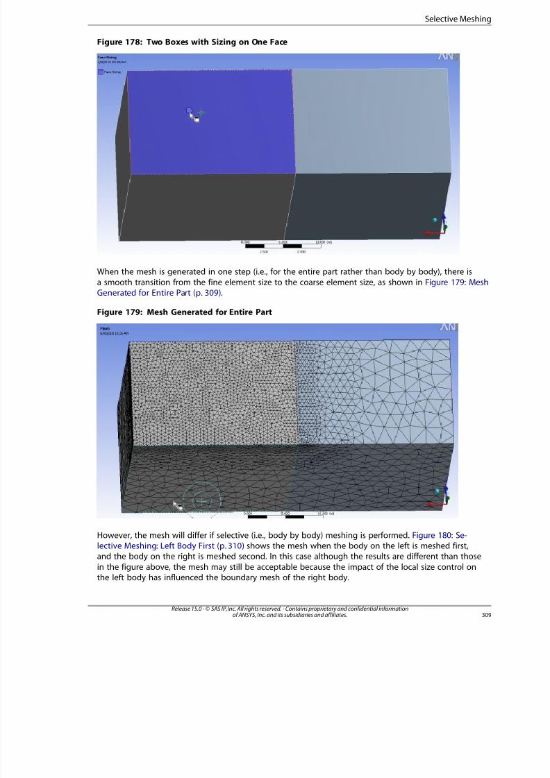
8/10/2019 ANSYS Meshing Users Guide
http://slidepdf.com/reader/full/ansys-meshing-users-guide 317/491
Figure 178: Two Boxes with Sizing on One Face
When the mesh is generated in one step (i.e., for the entire part rather than body by body), there is
a smooth transition from the fine element size to the coarse element size, as shown in Figure 179: MeshGenerated for Entire Part (p. 309).
Figure 179: Mesh Generated for Entire Part
However, the mesh will differ if selective (i.e., body by body) meshing is performed. Figure 180: Se-lective Meshing: Left Body First (p. 310) shows the mesh when the body on the left is meshed first,and the body on the right is meshed second. In this case although the results are different than those
in the figure above, the mesh may still be acceptable because the impact of the local size control onthe left body has influenced the boundary mesh of the right body.
309Release 15.0 - © SAS IP, Inc. All rights reserved. - Contains proprietary and confidential informationof ANSYS, Inc. and its subsidiaries and affiliates.
Selective Meshing
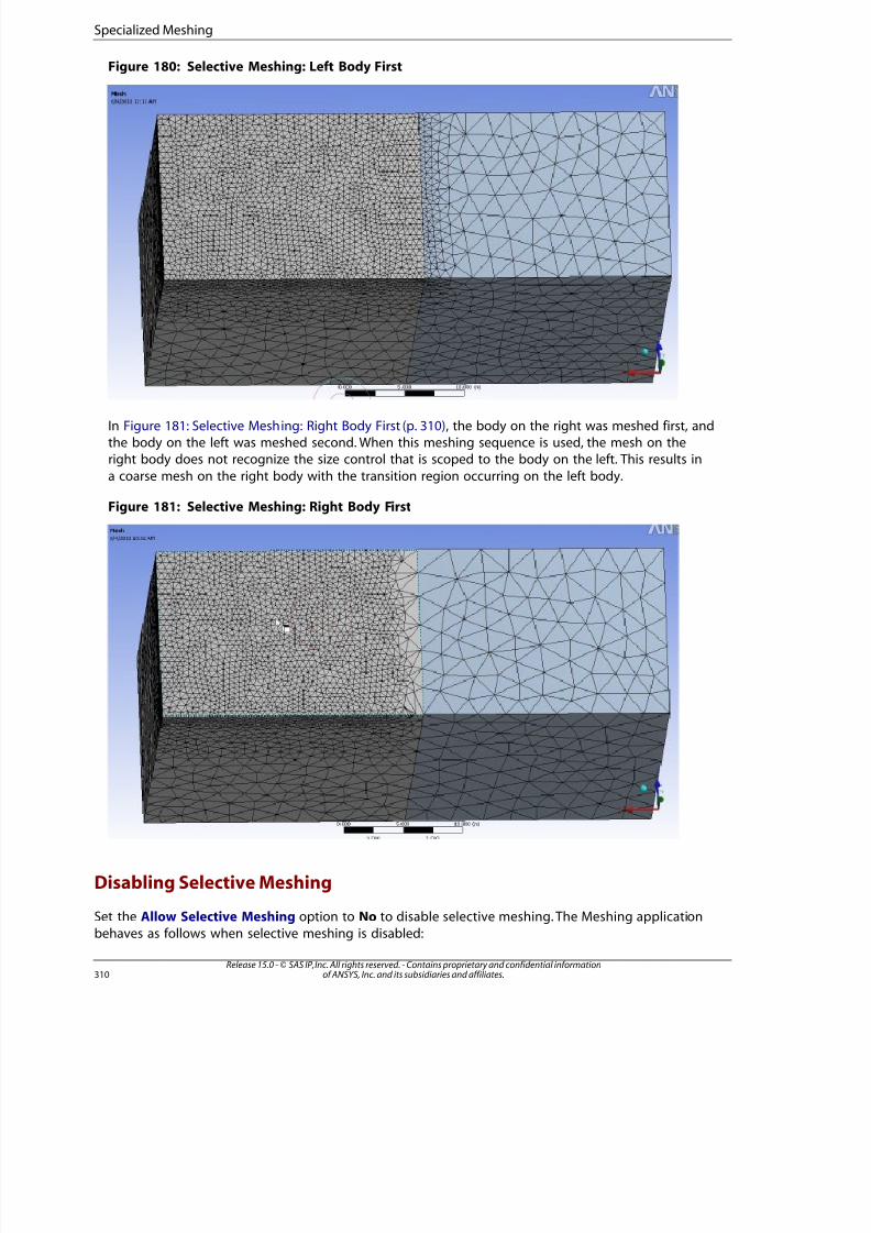
8/10/2019 ANSYS Meshing Users Guide
http://slidepdf.com/reader/full/ansys-meshing-users-guide 318/491
Figure 180: Selective Meshing: Left Body First
In Figure 181: Selective Meshing: Right Body First (p. 310), the body on the right was meshed first, andthe body on the left was meshed second. When this meshing sequence is used, the mesh on theright body does not recognize the size control that is scoped to the body on the left. This results in
a coarse mesh on the right body with the transition region occurring on the left body.
Figure 181: Selective Meshing: Right Body First
Disabling Selective Meshing
Set the Allow Selective Meshing option to No to disable selective meshing. The Meshing application
behaves as follows when selective meshing is disabled:
Release 15.0 - © SAS IP, Inc. All rights reserved. - Contains proprietary and confidential informationof ANSYS, Inc. and its subsidiaries and affiliates.310
Specialized Meshing

8/10/2019 ANSYS Meshing Users Guide
http://slidepdf.com/reader/full/ansys-meshing-users-guide 319/491
• If you make changes after meshing that invalidate the mesh for an individual body in a multibodypart (such as adding sizing to the body), the mesh for all bodies in the part is invalidated and you
will need to re-mesh all bodies.
• If one body in a multibody part is suppressed and you mesh all the other bodies, unsuppressing thesuppressed body invalidates the mesh for all the bodies within that part. When you regenerate the
mesh, all the bodies within that part will be re-meshed. If the model contains multiple parts, bodiesin the other parts will not be affected and will not be re-meshed.
• The Generate Mesh, Preview Surface Mesh, and Clear Generated Data RMB menu options are
unavailable for individual bodies in multibody parts in the Tree Outline. To use these features for amultibody part, you must right-click at the part level in the Tree Outline.
• There is no Parts> flyout menu for the Generate Mesh, Preview Surface Mesh, and Clear GeneratedData RMB menu options in the Geometry window. If you select one of these options, the action is
performed on the entire part.
Note
• In some cases, the mesh may be generated in a selective fashion (i.e., body by body) even if selective meshing is currently disabled. For example, if you use selective meshing to mesh
some of the bodies in a part, then disable selective meshing, and then generate the mesh and
the mesh process does not invalidate any bodies , the mesh is generated using selective meshingprocesses. To avoid this behavior, you can use the Clear Generated Data feature or force achange of the mesh state on the part. Non-selective meshing will be used for all subsequent
meshing.
• Mesh method interoperability is supported regardless of whether selective meshing is enabledor disabled. Refer to Conformal Meshing Between Parts (p. 5) for information about meshmethod interoperability.
Using the Mesh Worksheet to Create a Selective Meshing History
When you perform selective meshing, you control the sequence in which bodies are meshed. You canuse the Mesh worksheet to create a selective meshing history, so that your meshing steps can be re-peated in the desired sequence for any geometry update or re-mesh operation. Figure 182: MeshWorksheet (p. 312) shows a sample Mesh worksheet. Each row in the worksheet corresponds to a step
in the meshing sequence. When you generate the mesh, the software processes the steps one by one.For each step, the software selects the bodies identified by the specified Named Selection and meshesthose bodies using the meshing controls that are applied to them.
Note
The Mesh worksheet is a helpful meshing tool, but it does not manage mesh state. State
management is handled at the prototype (i.e., Body object) and mesh levels. Mesh state isvisible in the Tree Outline in the Geometry folder and in the Mesh folder. See UnderstandingStates (p. 394) for more information.
31Release 15.0 - © SAS IP, Inc. All rights reserved. - Contains proprietary and confidential informationof ANSYS, Inc. and its subsidiaries and affiliates.
Selective Meshing

8/10/2019 ANSYS Meshing Users Guide
http://slidepdf.com/reader/full/ansys-meshing-users-guide 320/491
Figure 182: Mesh Worksheet
There are two ways to create a selective meshing history:
• By recording meshing steps as you perform them
• By adding meshing steps to the worksheet manually
To create a selective meshing history by recording your steps:
1. Click the Mesh object in the Tree Outline.
2. Do one of the following:
Right-click the Mesh object and select Start Recording from the context menu. As a result, the
worksheet opens in recording mode automatically.-or-Click the Worksheet button on the toolbar and click the Start Recording button on the work-
sheet.
3. Move the worksheet to the desired location to dock it. The location will persist whenever the Mesh objector one of its child objects is highlighted in the Tree Outline. For example, you may want to dock theworksheet alongside the Geometry window, allowing you to view both at once.
Note
The worksheet is not dockable on Linux platforms. On Linux, you can drag the worksheetoff the Meshing application interface, and it will then appear in its own separate window.
4. Do one of the following:
Select one or more bodies or parts in the Geometry window, right-click, and select GenerateMesh on Selected Bodies. If you did not dock the worksheet, you may need to click theWorksheet button on the toolbar or the Graphics tab at the bottom of the worksheet to returnto the Geometry window first.
-or-Select one or more bodies or parts in the Tree Outline, right-click, and select Generate Mesh.
As a result, a Named Selection for the selected set is generated (named Meshing_1, Meshing_2,
Meshing_3, and so on) and is added to the worksheet automatically.
Release 15.0 - © SAS IP, Inc. All rights reserved. - Contains proprietary and confidential informationof ANSYS, Inc. and its subsidiaries and affiliates.312
Specialized Meshing

8/10/2019 ANSYS Meshing Users Guide
http://slidepdf.com/reader/full/ansys-meshing-users-guide 321/491
During recording, other steps in the worksheet are ignored while the mesh for the selected set isbeing generated. See below for additional notes on recording and playback behaviors.
5. Repeat step 4 for each meshing step in the desired sequence.
6. When you are done meshing bodies/parts, do one of the following:
Right-click the Mesh object and select Stop Recording from the context menu.
-or-Click the Stop Recording button on the worksheet.
Note
You do not have to record the meshing for all bodies, only those for which you want to
record the meshing order. See Mesh Worksheet Recording and Playback Behaviors (p. 313)for details.
To create a selective meshing history manually:
1. Click the Mesh object in the Tree Outline.
2. Click the Worksheet button on the toolbar.
3. Move the worksheet to the desired location to dock it. The location will persist whenever the Mesh objor one of its child objects is highlighted in the Tree Outline. For example, you may want to dock the
worksheet alongside the Geometry window, allowing you to view both at once.
Note
The worksheet is not dockable on Linux platforms. On Linux, you can drag the worksheet
off the Meshing application interface, and it will then appear in its own separate window.
4. Add a row to the worksheet by right-clicking on the table and selecting Add from the context menu.
5. In the new row, click on the Named Selection column and select a Named Selection from the NamedSelection drop-down.
6. Repeat steps 4 and 5 for each meshing step in the desired sequence.
Mesh Worksheet Recording and Playback Behaviors
Remember the following information regarding recording and playback behaviors:
• During recording, the button in the upper-right corner of the worksheet is red. When recording is stoppethe button is green.
• When you start recording, the software checks for meshed bodies and verifies that each meshed body isaccounted for in the worksheet. If any extraneous meshed bodies are found, recording does not occurand an error message is issued. You must clear the mesh entirely (or at least clear the mesh from thebodies that are not being used by the worksheet) before you can begin recording. To do so, use the Clea
Generated Data option or click the Clear Generated Mesh button on the worksheet.
313Release 15.0 - © SAS IP, Inc. All rights reserved. - Contains proprietary and confidential informationof ANSYS, Inc. and its subsidiaries and affiliates.
Selective Meshing
8/10/2019 ANSYS Meshing Users Guide
http://slidepdf.com/reader/full/ansys-meshing-users-guide 322/491
• When you start recording, the states of the bodies being used by the worksheet are checked. If any bodyis not in a meshed state, recording does not occur and an error message is issued. You must bring the
mesh up-to-date before you can begin recording. To do so, right-click on the last step in the worksheetand select Generate Mesh Through This Step from the context menu. See below for more informationabout using this option.
• As steps are being recorded, they are appended to the existing steps in the worksheet.
• Other steps in the worksheet are ignored while the mesh for the selected set is being generated.
• After you have entered recording mode, recording stops when the mesh is up-to-date. An exception to
this behavior occurs if you record one or more steps but then suppress all remaining unmeshed bodies.In such cases, the mesh will be up-to-date but recording will not stop automatically. You must click StopRecording.
• During recording/playback, post mesh operations (including mesh connections, post pinch controls, post
inflation, and refinement) do not occur until the last step in the worksheet, after all meshing is complete.
• If you select the Preview Surface Mesh, Preview Source and Target Mesh, or Preview Inflation feature, re-cording stops and a warning message is issued.
• The Generate Mesh option is context sensitive. It behaves differently depending on where you invoke it.If you invoke it from the Mesh object in the Tree Outline (RMB on Mesh folder > Generate Mesh), it be-haves similar to the Preview options in that recording stops. If you invoke it from the Geometry object
(RMB on Geometry folder > Generate Mesh) or from the Geometry window (RMB > Generate Mesh OnSelected Bodies), the operation is treated as a selective meshing step and is recorded.
• If you insert a step manually, recording stops and a warning message is issued.
• If you delete a step manually, recording stops and a warning message is issued.
• If the mesh fails, recording stops and a warning message is issued.
• To replay steps incrementally, right-click in the row of interest and select Generate Mesh Through ThisStep from the context menu. As a result, recording stops, any existing mesh is cleared, and all meshing
steps prior to and including the selected step are replayed in the Geometry window.
Mesh Worksheet Named Selection Behaviors
Remember the following information regarding Named Selection behaviors:
• Only Named Selections that consist of bodies are selectable from the worksheet's Named Selection drop-down.
• If the model contains bodies that are not included in any Named Selection, these bodies are meshed last.
• If a Named Selection is used by the worksheet, the Used by Mesh Worksheet field in the Details Viewfor that Named Selection is set to Yes, even if the corresponding worksheet step is inactive.
• For Named Selections that are generated automatically by the worksheet, the Send to Solver option inthe Details View is set to No by default. The default is Yes for Named Selections that you create. Theworksheet respects the user-defined settings. That is, if you create a Named Selection, retain the Send toSolver setting of Yes, and subsequently use that Named Selection in the worksheet, the Named Selection
will be passed to the solver as expected.
Release 15.0 - © SAS IP, Inc. All rights reserved. - Contains proprietary and confidential informationof ANSYS, Inc. and its subsidiaries and affiliates.314
Specialized Meshing
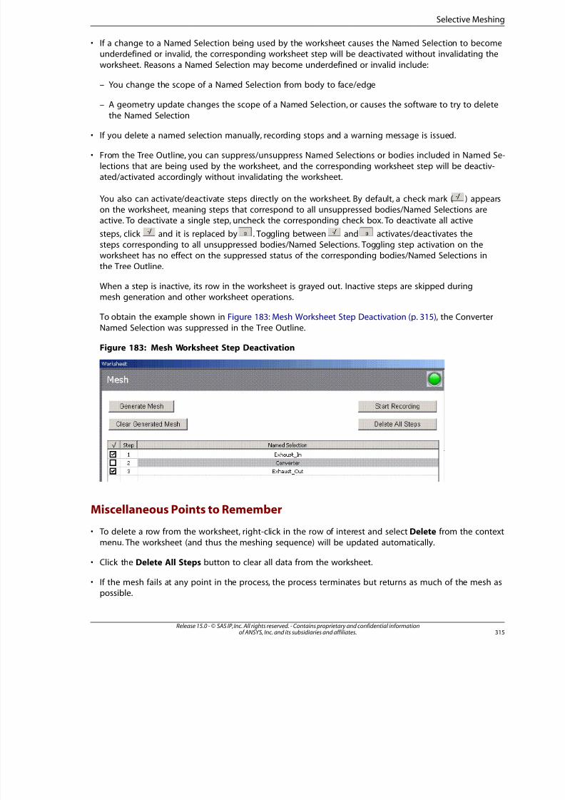
8/10/2019 ANSYS Meshing Users Guide
http://slidepdf.com/reader/full/ansys-meshing-users-guide 323/491
• If a change to a Named Selection being used by the worksheet causes the Named Selection to becomeunderdefined or invalid, the corresponding worksheet step will be deactivated without invalidating the
worksheet. Reasons a Named Selection may become underdefined or invalid include:
– You change the scope of a Named Selection from body to face/edge
– A geometry update changes the scope of a Named Selection, or causes the software to try to delete
the Named Selection
• If you delete a named selection manually, recording stops and a warning message is issued.
• From the Tree Outline, you can suppress/unsuppress Named Selections or bodies included in Named Se-
lections that are being used by the worksheet, and the corresponding worksheet step will be deactiv-ated/activated accordingly without invalidating the worksheet.
You also can activate/deactivate steps directly on the worksheet. By default, a check mark ( ) appearson the worksheet, meaning steps that correspond to all unsuppressed bodies/Named Selections areactive. To deactivate a single step, uncheck the corresponding check box. To deactivate all active
steps, click and it is replaced by . Toggling between and activates/deactivates thesteps corresponding to all unsuppressed bodies/Named Selections. Toggling step activation on theworksheet has no effect on the suppressed status of the corresponding bodies/Named Selections in
the Tree Outline.
When a step is inactive, its row in the worksheet is grayed out. Inactive steps are skipped duringmesh generation and other worksheet operations.
To obtain the example shown in Figure 183: Mesh Worksheet Step Deactivation (p. 315), the Converter
Named Selection was suppressed in the Tree Outline.
Figure 183: Mesh Worksheet Step Deactivation
Miscellaneous Points to Remember
• To delete a row from the worksheet, right-click in the row of interest and select Delete from the context
menu. The worksheet (and thus the meshing sequence) will be updated automatically.
• Click the Delete All Steps button to clear all data from the worksheet.
• If the mesh fails at any point in the process, the process terminates but returns as much of the mesh aspossible.
315Release 15.0 - © SAS IP, Inc. All rights reserved. - Contains proprietary and confidential informationof ANSYS, Inc. and its subsidiaries and affiliates.
Selective Meshing
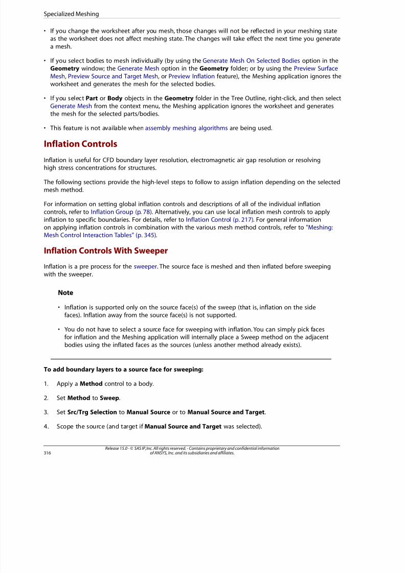
8/10/2019 ANSYS Meshing Users Guide
http://slidepdf.com/reader/full/ansys-meshing-users-guide 324/491
• If you change the worksheet after you mesh, those changes will not be reflected in your meshing stateas the worksheet does not affect meshing state. The changes will take effect the next time you generate
a mesh.
• If you select bodies to mesh individually (by using the Generate Mesh On Selected Bodies option in theGeometry window; the Generate Mesh option in the Geometry folder; or by using the Preview Surface
Mesh, Preview Source and Target Mesh, or Preview Inflation feature), the Meshing application ignores theworksheet and generates the mesh for the selected bodies.
• If you select Part or Body objects in the Geometry folder in the Tree Outline, right-click, and then select
Generate Mesh from the context menu, the Meshing application ignores the worksheet and generatesthe mesh for the selected parts/bodies.
• This feature is not available when assembly meshing algorithms are being used.
Inflation Controls
Inflation is useful for CFD boundary layer resolution, electromagnetic air gap resolution or resolvinghigh stress concentrations for structures.
The following sections provide the high-level steps to follow to assign inflation depending on the selectedmesh method.
For information on setting global inflation controls and descriptions of all of the individual inflation
controls, refer to Inflation Group (p. 78). Alternatively, you can use local inflation mesh controls to applyinflation to specific boundaries. For details, refer to Inflation Control (p. 217). For general informationon applying inflation controls in combination with the various mesh method controls, refer to "Meshing:Mesh Control Interaction Tables" (p. 345).
Inflation Controls With Sweeper
Inflation is a pre process for the sweeper. The source face is meshed and then inflated before sweepingwith the sweeper.
Note
• Inflation is supported only on the source face(s) of the sweep (that is, inflation on the sidefaces). Inflation away from the source face(s) is not supported.
• You do not have to select a source face for sweeping with inflation. You can simply pick facesfor inflation and the Meshing application will internally place a Sweep method on the adjacentbodies using the inflated faces as the sources (unless another method already exists).
To add boundary layers to a source face for sweeping:
1. Apply a Method control to a body.
2. Set Method to Sweep.
3. Set Src/Trg Selection to Manual Source or to Manual Source and Target.
4. Scope the source (and target if Manual Source and Target was selected).
Release 15.0 - © SAS IP, Inc. All rights reserved. - Contains proprietary and confidential informationof ANSYS, Inc. and its subsidiaries and affiliates.316
Specialized Meshing
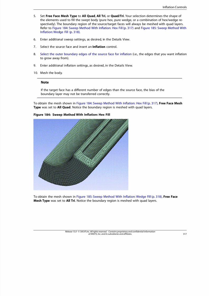
8/10/2019 ANSYS Meshing Users Guide
http://slidepdf.com/reader/full/ansys-meshing-users-guide 325/491
5. Set Free Face Mesh Type to All Quad, All Tri, or Quad/Tri. Your selection determines the shape of the elements used to fill the swept body (pure hex, pure wedge, or a combination of hex/wedge re-
spectively). The boundary region of the source/target faces will always be meshed with quad layers.Refer to Figure 184: Sweep Method With Inflation: Hex Fill (p. 317) and Figure 185: Sweep Method WithInflation: Wedge Fill (p. 318).
6. Enter additional sweep settings, as desired, in the Details View.
7. Select the source face and insert an Inflation control.
8. Select the outer boundary edges of the source face for inflation (i.e., the edges that you want inflation
to grow away from).
9. Enter additional inflation settings, as desired, in the Details View.
10. Mesh the body.
Note
If the target face has a different number of edges than the source face, the bias of the
boundary layer may not be transferred correctly.
To obtain the mesh shown in Figure 184: Sweep Method With Inflation: Hex Fill (p. 317), Free Face MeshType was set to All Quad. Notice the boundary region is meshed with quad layers.
Figure 184: Sweep Method With Inflation: Hex Fill
To obtain the mesh shown in Figure 185: Sweep Method With Inflation: Wedge Fill (p. 318), Free FaceMesh Type was set to All Tri. Notice the boundary region is meshed with quad layers.
317Release 15.0 - © SAS IP, Inc. All rights reserved. - Contains proprietary and confidential informationof ANSYS, Inc. and its subsidiaries and affiliates.
Inflation Controls

8/10/2019 ANSYS Meshing Users Guide
http://slidepdf.com/reader/full/ansys-meshing-users-guide 326/491
Figure 185: Sweep Method With Inflation: Wedge Fill
Inflation Controls With Patch Conforming Mesher
Inflation can be either a pre process or a post process for the patch conforming mesher.
To add boundary layers to a face using the Patch Conforming Mesher:
1. Apply a Method control to a body.
2. Set Method to Tetrahedrons.
3. Set the tetrahedrons Algorithm to Patch Conforming.
4. Select the body and insert an Inflation control.
5. Select the faces to be inflated (i.e., the faces that you want the inflation layers to grow away from).
6. Enter additional settings, as desired, in the Details View.
7. Mesh the body.
Inflation Controls With Patch Independent Mesher
Inflation is a post process for the patch independent mesher after it has created the tetrahedron elements.
To add boundary layers to a face using the Patch Independent Mesher:
1. Apply a Method control to a body.
2. Set Method to Tetrahedrons.
3. Set the tetrahedrons Algorithm to Patch Independent.
4. Set the Min Size Limit.
Release 15.0 - © SAS IP, Inc. All rights reserved. - Contains proprietary and confidential informationof ANSYS, Inc. and its subsidiaries and affiliates.318
Specialized Meshing

8/10/2019 ANSYS Meshing Users Guide
http://slidepdf.com/reader/full/ansys-meshing-users-guide 327/491
5. Select the body and insert an Inflation control.
6. Select the faces to be inflated (i.e., the faces that you want the inflation layers to grow away from).
7. Enter additional settings, as desired, in the Details View.
8. Mesh the body.
Inflation Controls With MultiZone
To add boundary layers to a face using the MultiZone Mesher:
1. Apply a Method control to a body.
2. Set Method to MultiZone.
3. Select the body and insert an Inflation control.
4. Select the faces to be inflated (i.e., the faces that you want the inflation layers to grow away from).
5. Enter additional settings, as desired, in the Details View.
6. Mesh the body.
For more information, see MultiZone Support for Inflation (p. 270).
Inflation Controls With MultiZone Quad/Tri Mesher
To add boundary layers to a face using the MultiZone Quad/Tri Mesher:
1. Apply a Method control to a body.
2. Set Method to MultiZone Quad/Tri.
3. Select a body or face and insert an Inflation control.
4. Select the edges to be inflated (i.e., the edges that you want inflation to grow away from).
5. Enter additional settings, as desired, in the Details View.
6. Mesh the body.
Note
Base mesh caching is not supported for MultiZone Quad/Tri, so a change to inflation controls
requires remeshing.
Inflation Controls With Quadrilateral Dominant or All Triangles Mesher
Inflation is a pre process for the quadrilateral dominant mesher or all triangles mesher.
To add boundary layers to a face using the Quadrilateral Dominant or All Triangles Mesher:
1. Apply a Method control to a body.
319Release 15.0 - © SAS IP, Inc. All rights reserved. - Contains proprietary and confidential informationof ANSYS, Inc. and its subsidiaries and affiliates.
Inflation Controls
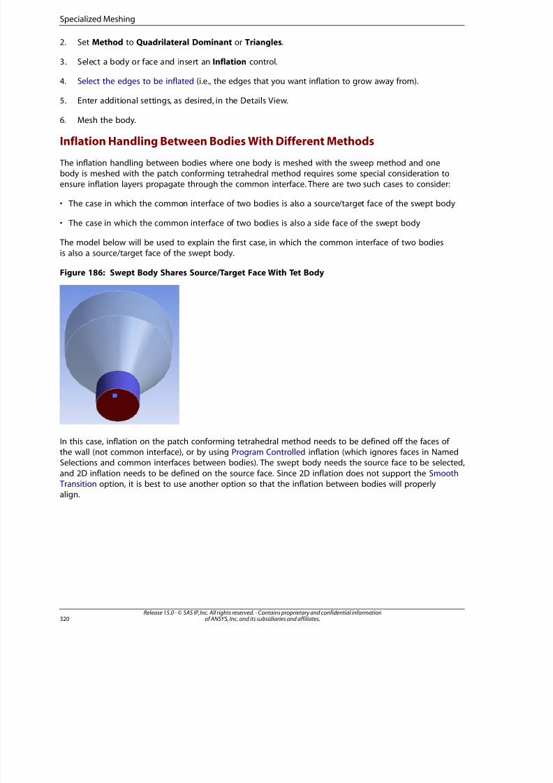
8/10/2019 ANSYS Meshing Users Guide
http://slidepdf.com/reader/full/ansys-meshing-users-guide 328/491
2. Set Method to Quadrilateral Dominant or Triangles.
3. Select a body or face and insert an Inflation control.
4. Select the edges to be inflated (i.e., the edges that you want inflation to grow away from).
5. Enter additional settings, as desired, in the Details View.
6. Mesh the body.
Inflation Handling Between Bodies With Different Methods
The inflation handling between bodies where one body is meshed with the sweep method and onebody is meshed with the patch conforming tetrahedral method requires some special consideration toensure inflation layers propagate through the common interface. There are two such cases to consider:
• The case in which the common interface of two bodies is also a source/target face of the swept body
• The case in which the common interface of two bodies is also a side face of the swept body
The model below will be used to explain the first case, in which the common interface of two bodiesis also a source/target face of the swept body.
Figure 186: Swept Body Shares Source/Target Face With Tet Body
In this case, inflation on the patch conforming tetrahedral method needs to be defined off the faces of the wall (not common interface), or by using Program Controlled inflation (which ignores faces in NamedSelections and common interfaces between bodies). The swept body needs the source face to be selected,
and 2D inflation needs to be defined on the source face. Since 2D inflation does not support the Smooth Transition option, it is best to use another option so that the inflation between bodies will properly
align.
Release 15.0 - © SAS IP, Inc. All rights reserved. - Contains proprietary and confidential informationof ANSYS, Inc. and its subsidiaries and affiliates.320
Specialized Meshing
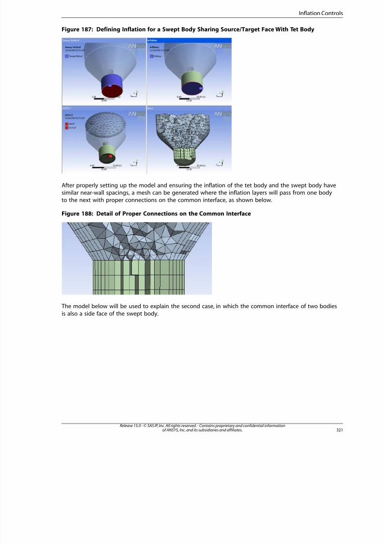
8/10/2019 ANSYS Meshing Users Guide
http://slidepdf.com/reader/full/ansys-meshing-users-guide 329/491
Figure 187: Defining Inflation for a Swept Body Sharing Source/Target Face With Tet Body
After properly setting up the model and ensuring the inflation of the tet body and the swept body havesimilar near-wall spacings, a mesh can be generated where the inflation layers will pass from one bodyto the next with proper connections on the common interface, as shown below.
Figure 188: Detail of Proper Connections on the Common Interface
The model below will be used to explain the second case, in which the common interface of two bodies
is also a side face of the swept body.
32Release 15.0 - © SAS IP, Inc. All rights reserved. - Contains proprietary and confidential informationof ANSYS, Inc. and its subsidiaries and affiliates.
Inflation Controls
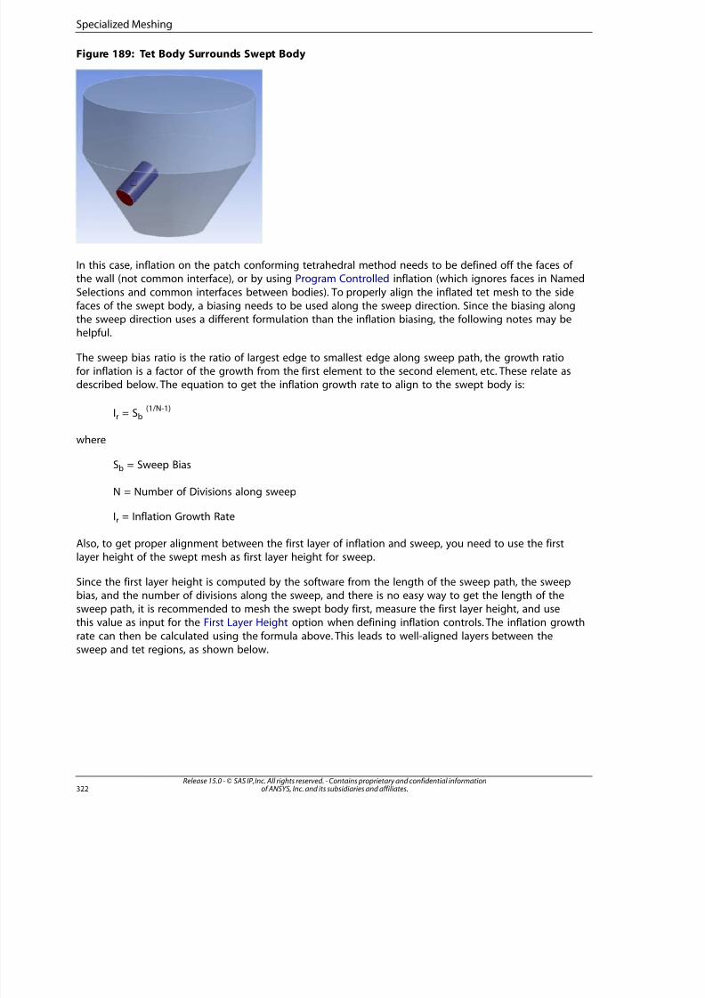
8/10/2019 ANSYS Meshing Users Guide
http://slidepdf.com/reader/full/ansys-meshing-users-guide 330/491
Figure 189: Tet Body Surrounds Swept Body
In this case, inflation on the patch conforming tetrahedral method needs to be defined off the faces of the wall (not common interface), or by using Program Controlled inflation (which ignores faces in Named
Selections and common interfaces between bodies). To properly align the inflated tet mesh to the sidefaces of the swept body, a biasing needs to be used along the sweep direction. Since the biasing alongthe sweep direction uses a different formulation than the inflation biasing, the following notes may behelpful.
The sweep bias ratio is the ratio of largest edge to smallest edge along sweep path, the growth ratiofor inflation is a factor of the growth from the first element to the second element, etc. These relate asdescribed below. The equation to get the inflation growth rate to align to the swept body is:
Ir = Sb(1/N-1)
where
Sb = Sweep Bias
N = Number of Divisions along sweep
Ir = Inflation Growth Rate
Also, to get proper alignment between the first layer of inflation and sweep, you need to use the firstlayer height of the swept mesh as first layer height for sweep.
Since the first layer height is computed by the software from the length of the sweep path, the sweepbias, and the number of divisions along the sweep, and there is no easy way to get the length of thesweep path, it is recommended to mesh the swept body first, measure the first layer height, and use
this value as input for the First Layer Height option when defining inflation controls. The inflation growthrate can then be calculated using the formula above. This leads to well-aligned layers between thesweep and tet regions, as shown below.
Release 15.0 - © SAS IP, Inc. All rights reserved. - Contains proprietary and confidential informationof ANSYS, Inc. and its subsidiaries and affiliates.322
Specialized Meshing
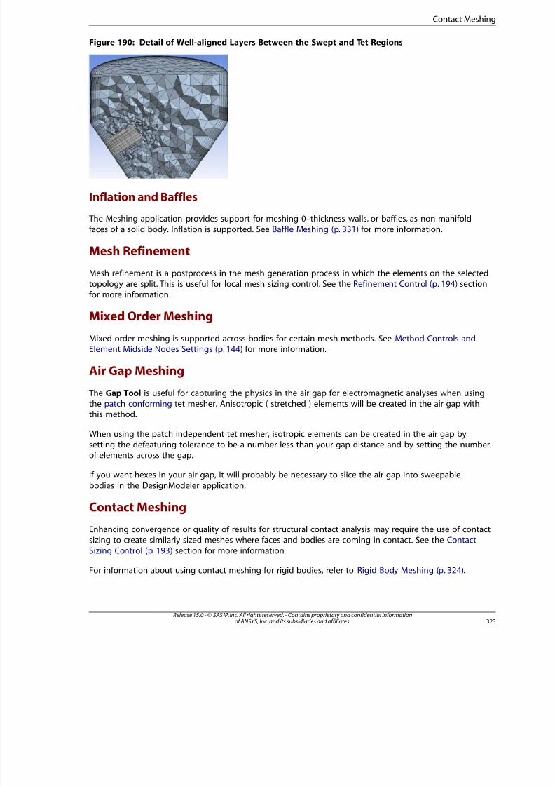
8/10/2019 ANSYS Meshing Users Guide
http://slidepdf.com/reader/full/ansys-meshing-users-guide 331/491
Figure 190: Detail of Well-aligned Layers Between the Swept and Tet Regions
Inflation and Baffles
The Meshing application provides support for meshing 0–thickness walls, or baffles, as non-manifoldfaces of a solid body. Inflation is supported. See Baffle Meshing (p. 331) for more information.
Mesh Refinement
Mesh refinement is a postprocess in the mesh generation process in which the elements on the selectedtopology are split. This is useful for local mesh sizing control. See the Refinement Control (p. 194) section
for more information.
Mixed Order Meshing
Mixed order meshing is supported across bodies for certain mesh methods. See Method Controls andElement Midside Nodes Settings (p. 144) for more information.
Air Gap Meshing
The Gap Tool is useful for capturing the physics in the air gap for electromagnetic analyses when usingthe patch conforming tet mesher. Anisotropic ( stretched ) elements will be created in the air gap withthis method.
When using the patch independent tet mesher, isotropic elements can be created in the air gap bysetting the defeaturing tolerance to be a number less than your gap distance and by setting the numberof elements across the gap.
If you want hexes in your air gap, it will probably be necessary to slice the air gap into sweepablebodies in the DesignModeler application.
Contact Meshing
Enhancing convergence or quality of results for structural contact analysis may require the use of contactsizing to create similarly sized meshes where faces and bodies are coming in contact. See the ContactSizing Control (p. 193) section for more information.
For information about using contact meshing for rigid bodies, refer to Rigid Body Meshing (p. 324).
323Release 15.0 - © SAS IP, Inc. All rights reserved. - Contains proprietary and confidential informationof ANSYS, Inc. and its subsidiaries and affiliates.
Contact Meshing
8/10/2019 ANSYS Meshing Users Guide
http://slidepdf.com/reader/full/ansys-meshing-users-guide 332/491
Winding Body Meshing
Winding body meshing creates special element types depending on the attributes given to bodies inthe DesignModeler application. No mesh controls are supported for winding bodies because of thenature of the required mesh.
Wire Body Meshing
Wire body meshing meshes the wire bodies in an assembly, respecting any mesh controls applied tothe edges of the wire body.
Pyramid Transitions
Pyramid transitions occur when a swept or hex dominant body abuts, that is, shares faces with, a body
meshed with tetrahedrons. The mesher will try to insert the pyramids into the body meshed with tetra-hedrons. If that is not possible, the hexahedron at the boundary will be split into pyramids and tetra-hedrons to create a conformal mesh between the two bodies. Pyramids will also be formed at the inter-face of an end cap of inflation on quad surface mesh and a tet body.
Match Meshing and the Symmetry Folder
Cyclic mesh matching, which controls mesh matching for a part that is symmetric about a cylindrical
axis, can be used for matching face meshes or matching edge meshes. When Periodic Region or CyclicRegion objects exist in the Symmetry folder, match face mesh controls will be created internal to themesher. If the mesher cannot match the mesh on the objects in the Symmetry folder, it will return afailure or informational message.
Related topics include:
• For a description of the Symmetry folder and its support of Periodic Region and Cyclic Region objects,
see Symmetry in the Mechanical help.
• For an overview of the cyclic match control, see Cyclic Match Control (p. 208).
• For an overview of the match control and its limitations, see Match Control (p. 206).
• For general information on applying match controls in combination with the various mesh method controls,
see "Meshing: Mesh Control Interaction Tables" (p. 345).
Rigid Body Meshing
Rigid body meshing simplifies the representation of a model by reducing it to the contact regions and
the centroid of the model. In other words, when a part is defined as a rigid body, the mesher knowsto mesh only the contact regions, and to create a single mass element at the centroid of the model.(The centroid is represented by an Inertial Coordinate System. Refer to the discussion of Rigid Bodies
in the Mechanical help for more information.)
Rigid body meshing can be used for both 2D and 3D contact. For 2D models, only the edges of the rigidsurface in contact are meshed because the surface mesh is not needed for the analysis. Similarly, for
3D models, only the faces of the rigid body in contact are meshed because the volume mesh is notneeded. The elements used to mesh the contact surfaces can be quadrilateral or triangular in shape,with or without midside nodes.
Release 15.0 - © SAS IP, Inc. All rights reserved. - Contains proprietary and confidential informationof ANSYS, Inc. and its subsidiaries and affiliates.324
Specialized Meshing
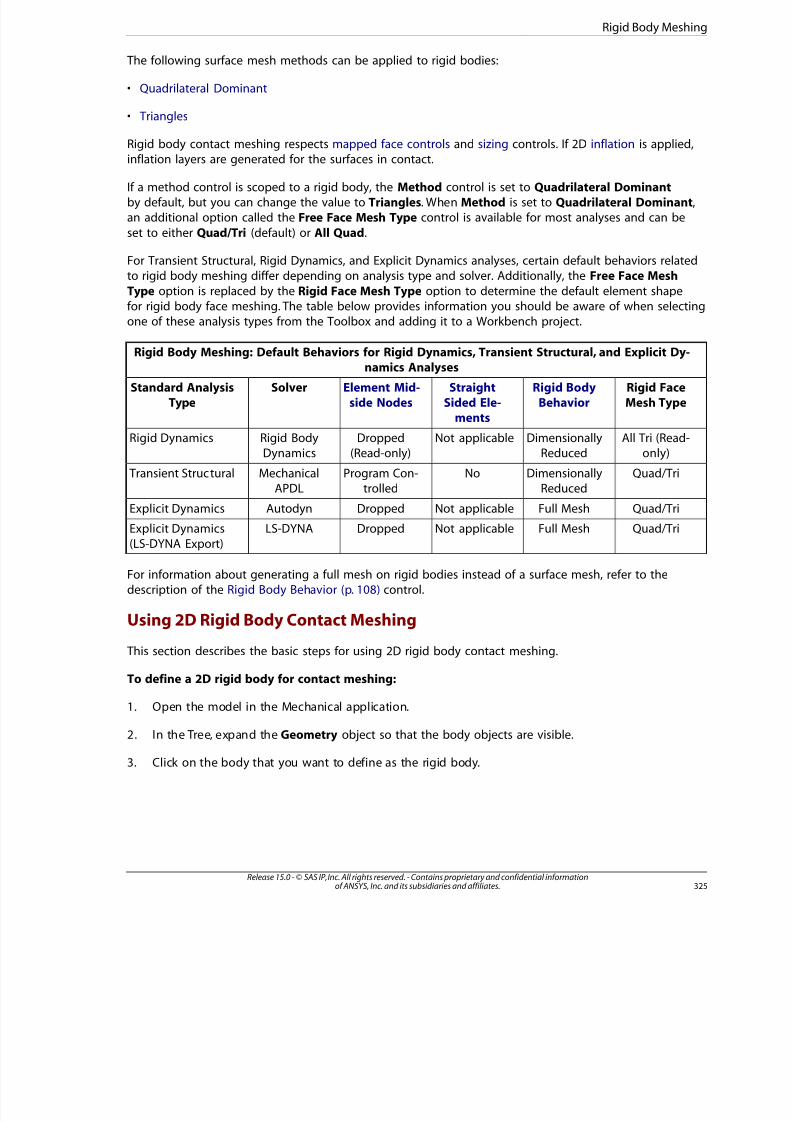
8/10/2019 ANSYS Meshing Users Guide
http://slidepdf.com/reader/full/ansys-meshing-users-guide 333/491
The following surface mesh methods can be applied to rigid bodies:
• Quadrilateral Dominant
• Triangles
Rigid body contact meshing respects mapped face controls and sizing controls. If 2D inflation is applied,inflation layers are generated for the surfaces in contact.
If a method control is scoped to a rigid body, the Method control is set to Quadrilateral Dominantby default, but you can change the value to Triangles. When Method is set to Quadrilateral Dominant,an additional option called the Free Face Mesh Type control is available for most analyses and can be
set to either Quad/Tri (default) or All Quad.
For Transient Structural, Rigid Dynamics, and Explicit Dynamics analyses, certain default behaviors relatedto rigid body meshing differ depending on analysis type and solver. Additionally, the Free Face Mesh
Type option is replaced by the Rigid Face Mesh Type option to determine the default element shapefor rigid body face meshing. The table below provides information you should be aware of when selectingone of these analysis types from the Toolbox and adding it to a Workbench project.
Rigid Body Meshing: Default Behaviors for Rigid Dynamics, Transient Structural, and Explicit Dy-namics Analyses
Rigid FaceMesh Type
Rigid BodyBehavior
StraightSided Ele-
ments
Element Mid-side Nodes
SolverStandard AnalysisType
All Tri (Read-only)
DimensionallyReduced
Not applicableDropped(Read-only)
Rigid BodyDynamics
Rigid Dynamics
Quad/TriDimensionallyReduced
NoProgram Con-trolled
MechanicalAPDL
Transient Structural
Quad/TriFull MeshNot applicableDroppedAutodynExplicit Dynamics
Quad/TriFull MeshNot applicableDroppedLS-DYNAExplicit Dynamics(LS-DYNA Export)
For information about generating a full mesh on rigid bodies instead of a surface mesh, refer to thedescription of the Rigid Body Behavior (p. 108) control.
Using 2D Rigid Body Contact Meshing
This section describes the basic steps for using 2D rigid body contact meshing.
To define a 2D rigid body for contact meshing:
1. Open the model in the Mechanical application.
2. In the Tree, expand the Geometry object so that the body objects are visible.
3. Click on the body that you want to define as the rigid body.
325Release 15.0 - © SAS IP, Inc. All rights reserved. - Contains proprietary and confidential informationof ANSYS, Inc. and its subsidiaries and affiliates.
Rigid Body Meshing
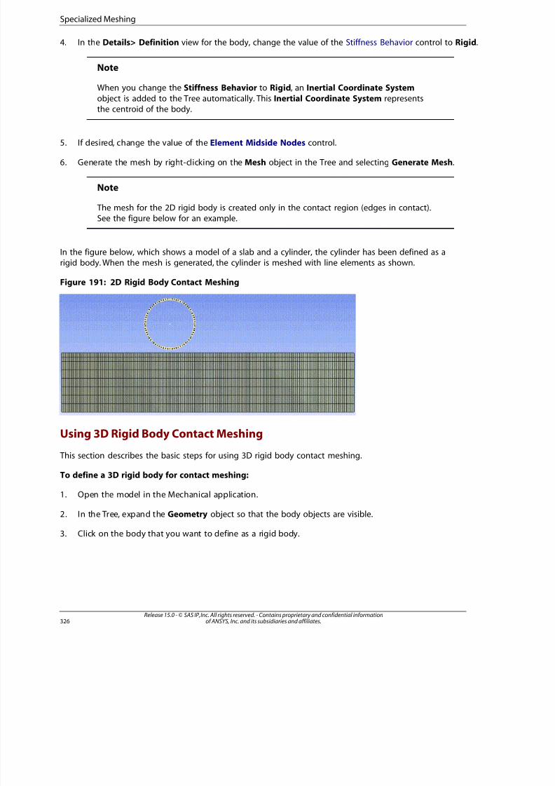
8/10/2019 ANSYS Meshing Users Guide
http://slidepdf.com/reader/full/ansys-meshing-users-guide 334/491
4. In the Details> Definition view for the body, change the value of the Stiffness Behavior control to Rigid.
Note
When you change the Stiffness Behavior to Rigid, an Inertial Coordinate System
object is added to the Tree automatically. This Inertial Coordinate System representsthe centroid of the body.
5. If desired, change the value of the Element Midside Nodes control.
6. Generate the mesh by right-clicking on the Mesh object in the Tree and selecting Generate Mesh.
Note
The mesh for the 2D rigid body is created only in the contact region (edges in contact).See the figure below for an example.
In the figure below, which shows a model of a slab and a cylinder, the cylinder has been defined as arigid body. When the mesh is generated, the cylinder is meshed with line elements as shown.
Figure 191: 2D Rigid Body Contact Meshing
Using 3D Rigid Body Contact Meshing
This section describes the basic steps for using 3D rigid body contact meshing.
To define a 3D rigid body for contact meshing:
1. Open the model in the Mechanical application.
2. In the Tree, expand the Geometry object so that the body objects are visible.
3. Click on the body that you want to define as a rigid body.
Release 15.0 - © SAS IP, Inc. All rights reserved. - Contains proprietary and confidential informationof ANSYS, Inc. and its subsidiaries and affiliates.326
Specialized Meshing

8/10/2019 ANSYS Meshing Users Guide
http://slidepdf.com/reader/full/ansys-meshing-users-guide 335/491
4. In the Details> Definition view for the body, change the value of the Stiffness Behavior control to Rig
Note
When you change the Stiffness Behavior to Rigid, an Inertial Coordinate System
object is added to the Tree automatically. This Inertial Coordinate System representsthe centroid of the body.
5. If you wish to control the mesh method, insert a mesh method by right-clicking on the Mesh object i
the Tree and selecting Insert> Method.
Note
The Automatic method appears in the Details View.
6. In the Details View, scope the mesh method to the rigid body.
Note
By default, the Method control is set to Quadrilateral Dominant for rigid bodies, but
you can change the value to Triangles. When Method is set to Quadrilateral Dominant,an additional option called the Free Face Mesh Type control is available and can beset to either Quad/Tri (default) or All Quad.
7. If desired, change the value of the Element Midside Nodes control.
8. Generate the mesh by right-clicking on the Mesh object in the Tree and selecting Generate Mesh.
Note
The mesh for the 3D rigid body is created only in the contact region (faces in contact).
Thin Solid Meshing
Thin solid meshing is useful for thin solid bodies where one element through the thickness is desired. This meshing also takes advantage of the Mechanical APDL application's SOLSH190 element.
• It may be advantageous to use a Sizing control on the faces/body along with Mapped Face Meshingcontrols to give a uniform mesh.
• Virtual Topology may be necessary to satisfy the topological criterion for thin solid meshing.
CAD Instance Meshing
The Meshing application supports pattern instances that have been defined for part features or assemblycomponents in a CAD system, such as Creo Parametric, Parasolid, or Solid Edge. These instance definitions
remain in the CAD system. When a model with instances is read in to Workbench, the geometry is read
327Release 15.0 - © SAS IP, Inc. All rights reserved. - Contains proprietary and confidential informationof ANSYS, Inc. and its subsidiaries and affiliates.
CAD Instance Meshing

8/10/2019 ANSYS Meshing Users Guide
http://slidepdf.com/reader/full/ansys-meshing-users-guide 336/491
once and then copied for each instance. Similarly, when meshing, the Meshing application generatesthe mesh once and then copies it for each instance. Support for pattern instances provides these benefits:
• Improved geometry import speed because only one instance of a part is read in
• Improved meshing speed because only one instance of a part is meshed; copies of the first instance'smesh are used for the remaining instances
Remember the following information when working with instances:
• Instances of bodies are not supported. Single body part instancing is supported, as well as certain variationsof instancing of multibody parts (for example, if you are using the None or Imprints option for Shared
Topology Method). For more information, refer to the discussion of feature modeling's effect on instancedata in the DesignModeler help.
• If you apply a mesh control to a part that is instanced, each instance must have the same control applied
to it or the part will be meshed individually. For example, if your model consists of four parts that are in-stanced but only one part has an edge sizing control applied to it, that part will be meshed individuallyand the other three parts will be meshed once and instanced.
• Instancing is not supported for the following controls. Each part that has any of these controls applied toit will be meshed individually, regardless of whether the control in question is applied to all instances:
– Sphere of influence sizing
– Body of influence sizing
– Contact sizing
– Gap sizing
– Match controls
– Rigid body meshing (presence of any rigid bodies in the part)
– Mesh morphing
• You can use the Extend Selection command to select a set of instances, which can be useful for performing
tasks such as applying loads or creating a Named Selection. To select a set of instances, first select oneinstance, then click the Extend Selection drop-down menu and choose Extend to Instances. Extend toInstances searches for all remaining instances that are defined for the currently selected instance. TheExtend to Instances menu option is enabled only when pattern instances are defined in the current
model.
• When using mesh methods or controls that require both body scoping and face scoping (such as Sweep
or MultiZone with source face selection; inflation; or match controls), you can use the Object Generatorto set up the model for instancing. For details, refer to Generating Multiple Objects from a Template Objectin the Mechanical help.
• Because the mesh is copied from the first instance to the remaining instance, it follows that each instance
will be meshed with the same number of nodes and elements. To confirm this, after CAD instances aresuccessfully meshed, click the Geometry object in the Tree Outline. Then click the Worksheet toolbarbutton. When the Worksheet appears, click on the Nodes heading, which sorts the data on that columnand allows you to view the matching numbers of nodes and elements for each instance.
Release 15.0 - © SAS IP, Inc. All rights reserved. - Contains proprietary and confidential informationof ANSYS, Inc. and its subsidiaries and affiliates.328
Specialized Meshing
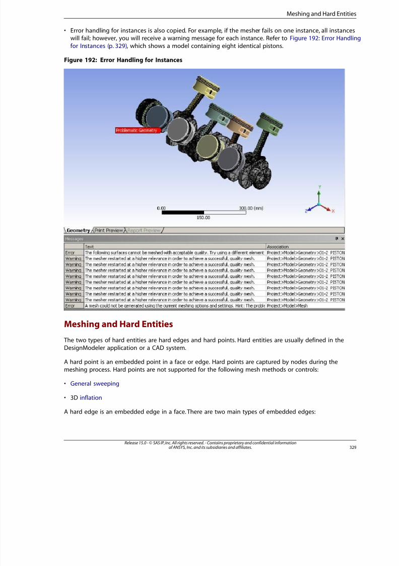
8/10/2019 ANSYS Meshing Users Guide
http://slidepdf.com/reader/full/ansys-meshing-users-guide 337/491
• Error handling for instances is also copied. For example, if the mesher fails on one instance, all instanceswill fail; however, you will receive a warning message for each instance. Refer to Figure 192: Error Handlin
for Instances (p. 329), which shows a model containing eight identical pistons.
Figure 192: Error Handling for Instances
Meshing and Hard Entities
The two types of hard entities are hard edges and hard points. Hard entities are usually defined in the
DesignModeler application or a CAD system.
A hard point is an embedded point in a face or edge. Hard points are captured by nodes during themeshing process. Hard points are not supported for the following mesh methods or controls:
• General sweeping
• 3D inflation
A hard edge is an embedded edge in a face. There are two main types of embedded edges:
329Release 15.0 - © SAS IP, Inc. All rights reserved. - Contains proprietary and confidential informationof ANSYS, Inc. and its subsidiaries and affiliates.
Meshing and Hard Entities
8/10/2019 ANSYS Meshing Users Guide
http://slidepdf.com/reader/full/ansys-meshing-users-guide 338/491
• An edge in which one vertex of the edge touches the face boundary, but the other vertex does nottouch a face boundary
• An edge in which neither of the vertices touches the face boundary
Hard edges are not supported for the following mesh methods or controls:
• General sweeping
• 2D or 3D inflation
Note
• If the methods and controls listed above are required in your mesh, you must go back to theDesignModeler application and edit the model to remove the hard entities.
• Other mesh methods have certain limitations in how hard points and hard edges are handled.For more information, refer to Limitations of Using Hard Entities with Other Mesh Controls (p. 330).
Spot Welds
Spot welds are used to connect individual surface body parts together to form surface body model as-semblies, just as contact is used for solid body part assemblies. Spot welds are usually defined as hard
points in the DesignModeler application or a CAD system:
• When a model is imported into the Meshing application, the mesher simply treats the hard pointsas embedded points.
• Upon import to the Mechanical application, spot welds are automatically generated where hard points
are defined in the model.
For related information, refer to Point in the DesignModeler help and Spot Welds in the Mechanicalhelp.
Limitations of Using Hard Entities with Other Mesh Controls
Limitations of hard entities include the following:
• 3D inflation does not support hard entities of either type. If inflation is applied, a warning messageis issued to indicate the hard entities were ignored.
• 2D inflation supports hard points only.
• General Sweeping does not support hard points.
• The MultiZone Quad/Tri and MultiZone mesh methods do not respect hard entities unless their topo-logy is protected. For all three methods, “protected topology” includes embedded vertices or edges
with contacts, Named Selections, loads, boundary conditions, or results; spot welds; or surface bodieswith differing thicknesses. For MultiZone Quad/Tri only, sheet bodies with differing material definitionsare also protected topology. The boundaries at protected topology will not be crossed.
• For the MultiZone mesh method only, the faces that contain the hard entities must be selected as
source faces for the hard entities to be respected.
Release 15.0 - © SAS IP, Inc. All rights reserved. - Contains proprietary and confidential informationof ANSYS, Inc. and its subsidiaries and affiliates.330
Specialized Meshing

8/10/2019 ANSYS Meshing Users Guide
http://slidepdf.com/reader/full/ansys-meshing-users-guide 339/491
• Hard edges may exist accidentally in a CAD model due to Boolean operations with tight tolerancesor other such operations. These accidental hard edges may be undesired, in which case you should
remove them through defeaturing within the DesignModeler application or a CAD system.
Baffle Meshing
The Meshing application provides support for meshing 0-thickness walls, or baffles, as non-manifoldfaces of a solid body. For such models, you do not have to adjust the mesh size to capture the thin re-gions.
Characteristics and limitations of baffle meshing include:
• For part/body level meshing, baffle meshing is supported by the Patch Conforming Tetra, Patch Inde-pendent Tetra, and MultiZone mesh methods only. If you apply any other mesh method to a bodycontaining baffles, the mesh method will be suppressed, and the reason (not supported) will be re-
ported in the Active read-only field in the Details View. In such cases, the body will be meshed withthe Patch Conforming Tetra mesh method.
Baffle meshing is also supported for assembly meshing algorithms. See Assembly Meshing (p. 273).
• When the MultiZone mesh method is used, the body with a baffle must be meshed with a free meshof tetrahedral elements. For this reason, you must set the Free Mesh Type to Tetra for bodies withbaffles.
• The Patch Conforming Tetra and Patch Independent Tetra mesh methods support inflation of baffles. The MultiZone mesh method does not support inflation of baffles.
• When the Patch Conforming Tetra mesh method is used, inflation layers will stair step at freeboundary edges of the baffles.
• When the Patch Independent Tetra mesh method is used and Collision Avoidance (p. 90) is set toStair Stepping, inflation layers will stair step at free boundary edges of the baffles. However, if Col-
lision Avoidance is set to Layer Compression, full prism columns appear at the free boundary edges.
• Program Controlled inflation is supported (that is, if you select Program Controlled inflation, bafflesare automatically selected to be inflation boundaries unless they are in a Named Selection).
• Only two-sided growth cases for inflation are supported.
• Pyramid transitions are supported.
• Prism/pyramid elements are not supported for meshing crossed/intersecting baffles.
• There is a single set of nodes on the internal face.
Figure 193: Cylinder Containing Baffles (p. 332) shows a model of a cylinder that contains a series of baffles.
33Release 15.0 - © SAS IP, Inc. All rights reserved. - Contains proprietary and confidential informationof ANSYS, Inc. and its subsidiaries and affiliates.
Baffle Meshing
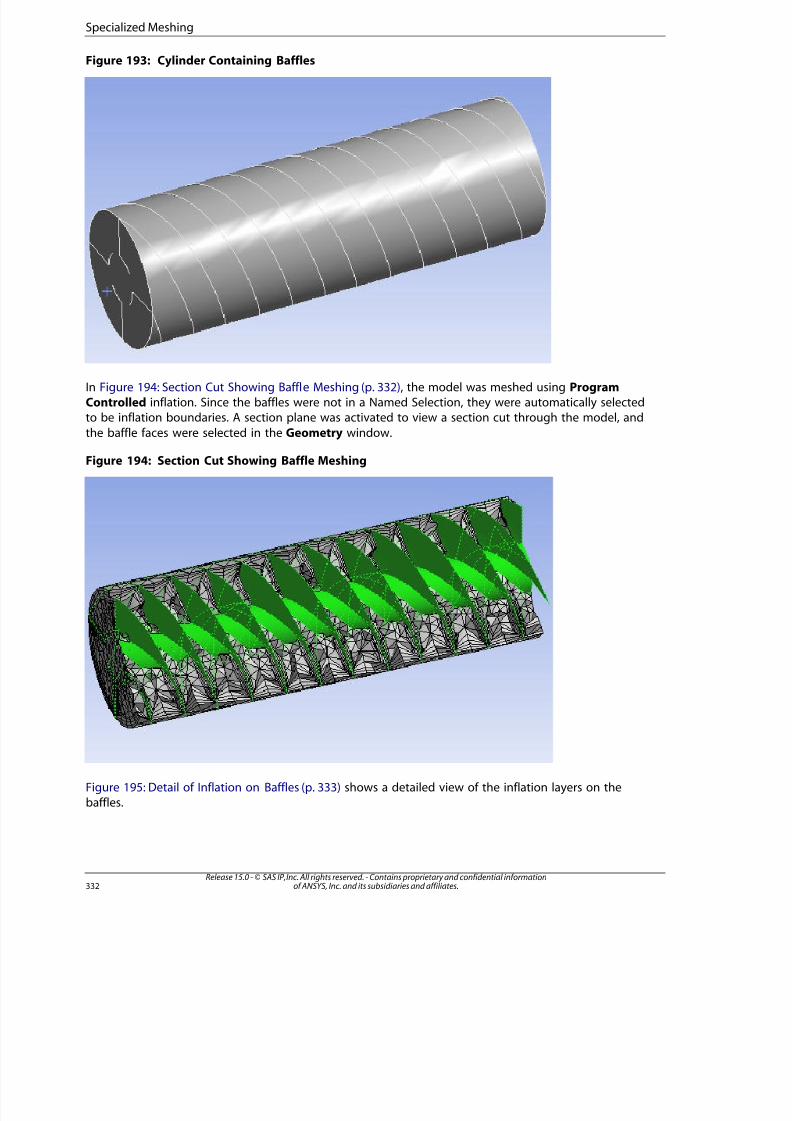
8/10/2019 ANSYS Meshing Users Guide
http://slidepdf.com/reader/full/ansys-meshing-users-guide 340/491
Figure 193: Cylinder Containing Baffles
In Figure 194: Section Cut Showing Baffle Meshing (p. 332), the model was meshed using ProgramControlled inflation. Since the baffles were not in a Named Selection, they were automatically selectedto be inflation boundaries. A section plane was activated to view a section cut through the model, and
the baffle faces were selected in the Geometry window.
Figure 194: Section Cut Showing Baffle Meshing
Figure 195: Detail of Inflation on Baffles (p. 333) shows a detailed view of the inflation layers on thebaffles.
Release 15.0 - © SAS IP, Inc. All rights reserved. - Contains proprietary and confidential informationof ANSYS, Inc. and its subsidiaries and affiliates.332
Specialized Meshing
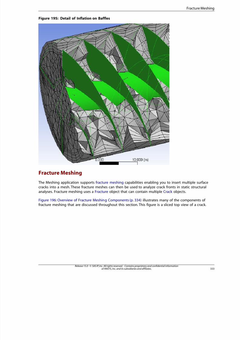
8/10/2019 ANSYS Meshing Users Guide
http://slidepdf.com/reader/full/ansys-meshing-users-guide 341/491
Figure 195: Detail of Inflation on Baffles
Fracture Meshing
The Meshing application supports fracture meshing capabilities enabling you to insert multiple surfacecracks into a mesh. These fracture meshes can then be used to analyze crack fronts in static structuralanalyses. Fracture meshing uses a Fracture object that can contain multiple Crack objects.
Figure 196: Overview of Fracture Meshing Components (p. 334) illustrates many of the components of fracture meshing that are discussed throughout this section. This figure is a sliced top view of a crack.
333Release 15.0 - © SAS IP, Inc. All rights reserved. - Contains proprietary and confidential informationof ANSYS, Inc. and its subsidiaries and affiliates.
Fracture Meshing
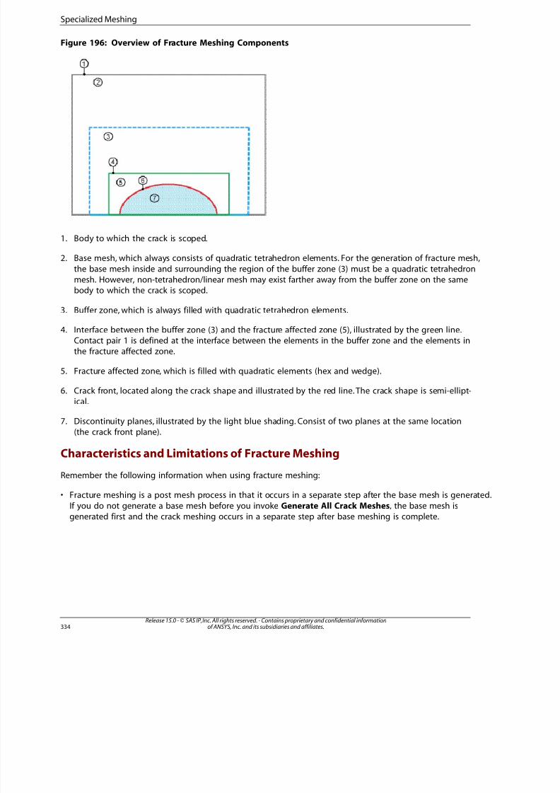
8/10/2019 ANSYS Meshing Users Guide
http://slidepdf.com/reader/full/ansys-meshing-users-guide 342/491
Figure 196: Overview of Fracture Meshing Components
1. Body to which the crack is scoped.
2. Base mesh, which always consists of quadratic tetrahedron elements. For the generation of fracture mesh,
the base mesh inside and surrounding the region of the buffer zone (3) must be a quadratic tetrahedronmesh. However, non-tetrahedron/linear mesh may exist farther away from the buffer zone on the samebody to which the crack is scoped.
3. Buffer zone, which is always filled with quadratic tetrahedron elements.
4. Interface between the buffer zone (3) and the fracture affected zone (5), illustrated by the green line.Contact pair 1 is defined at the interface between the elements in the buffer zone and the elements inthe fracture affected zone.
5. Fracture affected zone, which is filled with quadratic elements (hex and wedge).
6. Crack front, located along the crack shape and illustrated by the red line. The crack shape is semi-ellipt-ical.
7. Discontinuity planes, illustrated by the light blue shading. Consist of two planes at the same location(the crack front plane).
Characteristics and Limitations of Fracture Meshing
Remember the following information when using fracture meshing:
• Fracture meshing is a post mesh process in that it occurs in a separate step after the base mesh is generated.If you do not generate a base mesh before you invoke Generate All Crack Meshes, the base mesh isgenerated first and the crack meshing occurs in a separate step after base meshing is complete.
Release 15.0 - © SAS IP, Inc. All rights reserved. - Contains proprietary and confidential informationof ANSYS, Inc. and its subsidiaries and affiliates.334
Specialized Meshing
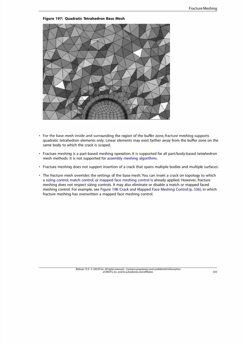
8/10/2019 ANSYS Meshing Users Guide
http://slidepdf.com/reader/full/ansys-meshing-users-guide 343/491
Figure 197: Quadratic Tetrahedron Base Mesh
• For the base mesh inside and surrounding the region of the buffer zone, fracture meshing supportsquadratic tetrahedron elements only. Linear elements may exist farther away from the buffer zone on thsame body to which the crack is scoped.
• Fracture meshing is a part-based meshing operation. It is supported for all part/body-based tetrahedronmesh methods. It is not supported for assembly meshing algorithms.
• Fracture meshing does not support insertion of a crack that spans multiple bodies and multiple surfaces
• The fracture mesh overrides the settings of the base mesh. You can insert a crack on topology to whicha sizing control, match control, or mapped face meshing control is already applied. However, fracturemeshing does not respect sizing controls. It may also eliminate or disable a match or mapped facedmeshing control. For example, see Figure 198: Crack and Mapped Face Meshing Control (p. 336), in which
fracture meshing has overwritten a mapped face meshing control.
335Release 15.0 - © SAS IP, Inc. All rights reserved. - Contains proprietary and confidential informationof ANSYS, Inc. and its subsidiaries and affiliates.
Fracture Meshing
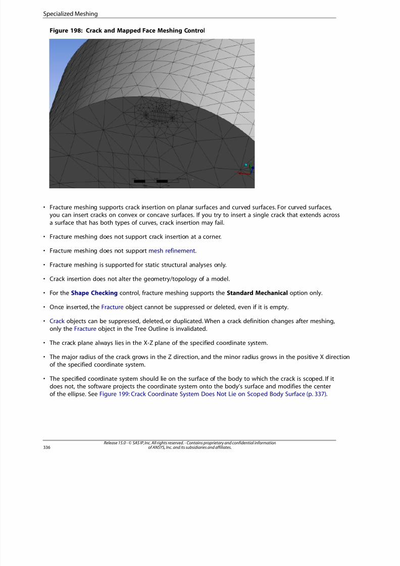
8/10/2019 ANSYS Meshing Users Guide
http://slidepdf.com/reader/full/ansys-meshing-users-guide 344/491
Figure 198: Crack and Mapped Face Meshing Control
• Fracture meshing supports crack insertion on planar surfaces and curved surfaces. For curved surfaces,you can insert cracks on convex or concave surfaces. If you try to insert a single crack that extends across
a surface that has both types of curves, crack insertion may fail.
• Fracture meshing does not support crack insertion at a corner.
• Fracture meshing does not support mesh refinement.
• Fracture meshing is supported for static structural analyses only.
• Crack insertion does not alter the geometry/topology of a model.
• For the Shape Checking control, fracture meshing supports the Standard Mechanical option only.
• Once inserted, the Fracture object cannot be suppressed or deleted, even if it is empty.
• Crack objects can be suppressed, deleted, or duplicated. When a crack definition changes after meshing,only the Fracture object in the Tree Outline is invalidated.
• The crack plane always lies in the X-Z plane of the specified coordinate system.
• The major radius of the crack grows in the Z direction, and the minor radius grows in the positive X directionof the specified coordinate system.
• The specified coordinate system should lie on the surface of the body to which the crack is scoped. If itdoes not, the software projects the coordinate system onto the body’s surface and modifies the centerof the ellipse. See Figure 199: Crack Coordinate System Does Not Lie on Scoped Body Surface (p. 337).
Release 15.0 - © SAS IP, Inc. All rights reserved. - Contains proprietary and confidential informationof ANSYS, Inc. and its subsidiaries and affiliates.336
Specialized Meshing
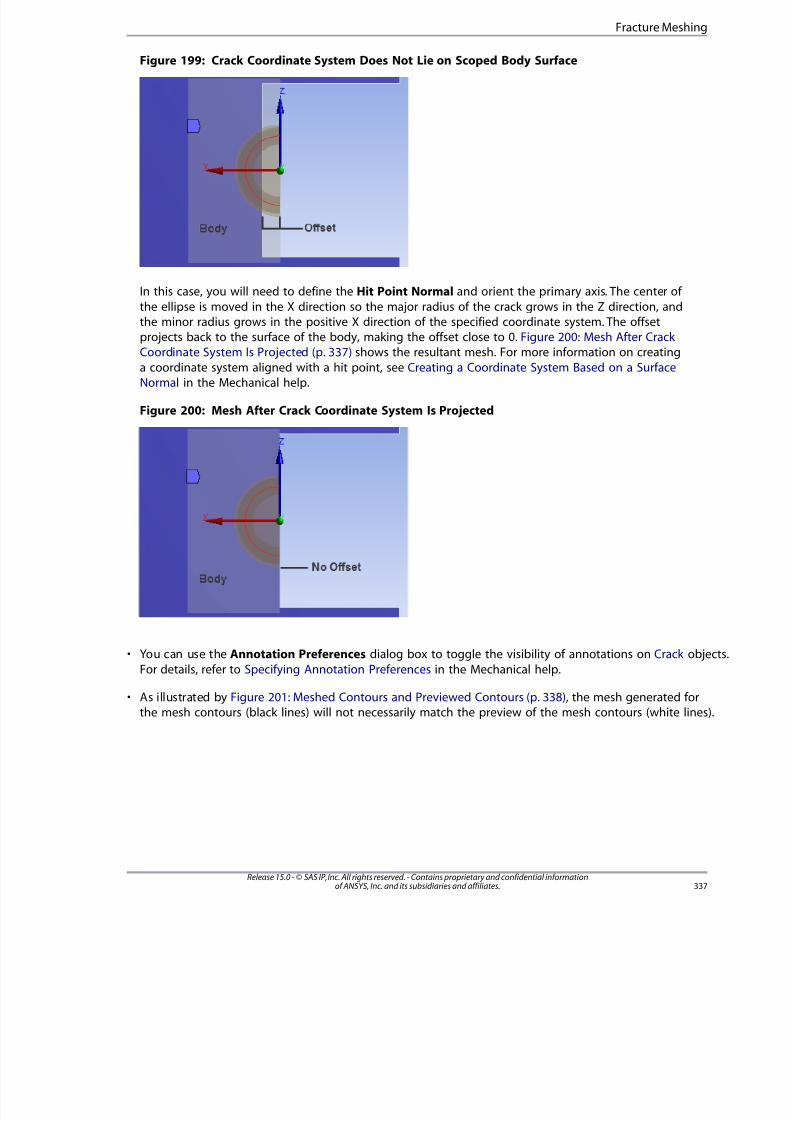
8/10/2019 ANSYS Meshing Users Guide
http://slidepdf.com/reader/full/ansys-meshing-users-guide 345/491
Figure 199: Crack Coordinate System Does Not Lie on Scoped Body Surface
In this case, you will need to define the Hit Point Normal and orient the primary axis. The center of
the ellipse is moved in the X direction so the major radius of the crack grows in the Z direction, andthe minor radius grows in the positive X direction of the specified coordinate system. The offsetprojects back to the surface of the body, making the offset close to 0. Figure 200: Mesh After Crack
Coordinate System Is Projected (p. 337) shows the resultant mesh. For more information on creatinga coordinate system aligned with a hit point, see Creating a Coordinate System Based on a SurfaceNormal in the Mechanical help.
Figure 200: Mesh After Crack Coordinate System Is Projected
• You can use the Annotation Preferences dialog box to toggle the visibility of annotations on Crack obj
For details, refer to Specifying Annotation Preferences in the Mechanical help.
• As illustrated by Figure 201: Meshed Contours and Previewed Contours (p. 338), the mesh generated forthe mesh contours (black lines) will not necessarily match the preview of the mesh contours (white lines
337Release 15.0 - © SAS IP, Inc. All rights reserved. - Contains proprietary and confidential informationof ANSYS, Inc. and its subsidiaries and affiliates.
Fracture Meshing
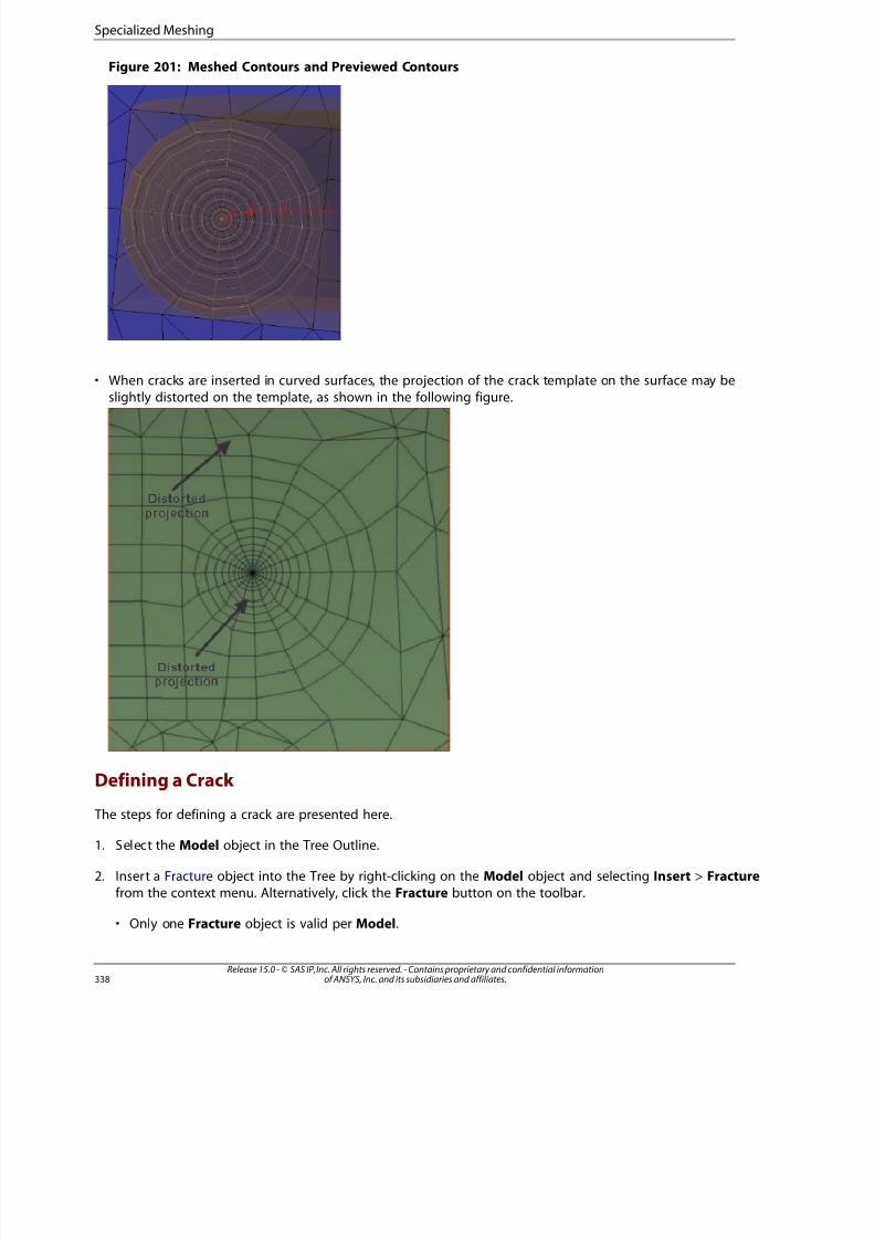
8/10/2019 ANSYS Meshing Users Guide
http://slidepdf.com/reader/full/ansys-meshing-users-guide 346/491
Figure 201: Meshed Contours and Previewed Contours
• When cracks are inserted in curved surfaces, the projection of the crack template on the surface may beslightly distorted on the template, as shown in the following figure.
Defining a Crack
The steps for defining a crack are presented here.
1. Select the Model object in the Tree Outline.
2. Insert a Fracture object into the Tree by right-clicking on the Model object and selecting Insert > Fracturefrom the context menu. Alternatively, click the Fracture button on the toolbar.
• Only one Fracture object is valid per Model.
Release 15.0 - © SAS IP, Inc. All rights reserved. - Contains proprietary and confidential informationof ANSYS, Inc. and its subsidiaries and affiliates.338
Specialized Meshing
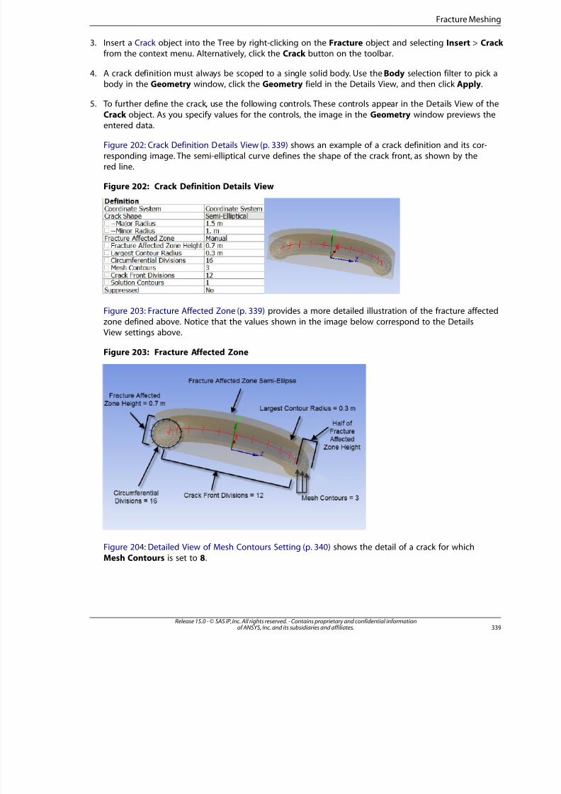
8/10/2019 ANSYS Meshing Users Guide
http://slidepdf.com/reader/full/ansys-meshing-users-guide 347/491
3. Insert a Crack object into the Tree by right-clicking on the Fracture object and selecting Insert > Cracfrom the context menu. Alternatively, click the Crack button on the toolbar.
4. A crack definition must always be scoped to a single solid body. Use the Body selection filter to pick abody in the Geometry window, click the Geometry field in the Details View, and then click Apply.
5. To further define the crack, use the following controls. These controls appear in the Details View of the
Crack object. As you specify values for the controls, the image in the Geometry window previews the
entered data.
Figure 202: Crack Definition Details View (p. 339) shows an example of a crack definition and its cor-
responding image. The semi-elliptical curve defines the shape of the crack front, as shown by thered line.
Figure 202: Crack Definition Details View
Figure 203: Fracture Affected Zone (p. 339) provides a more detailed illustration of the fracture affected
zone defined above. Notice that the values shown in the image below correspond to the DetailsView settings above.
Figure 203: Fracture Affected Zone
Figure 204: Detailed View of Mesh Contours Setting (p. 340) shows the detail of a crack for which
Mesh Contours is set to 8.
339Release 15.0 - © SAS IP, Inc. All rights reserved. - Contains proprietary and confidential informationof ANSYS, Inc. and its subsidiaries and affiliates.
Fracture Meshing
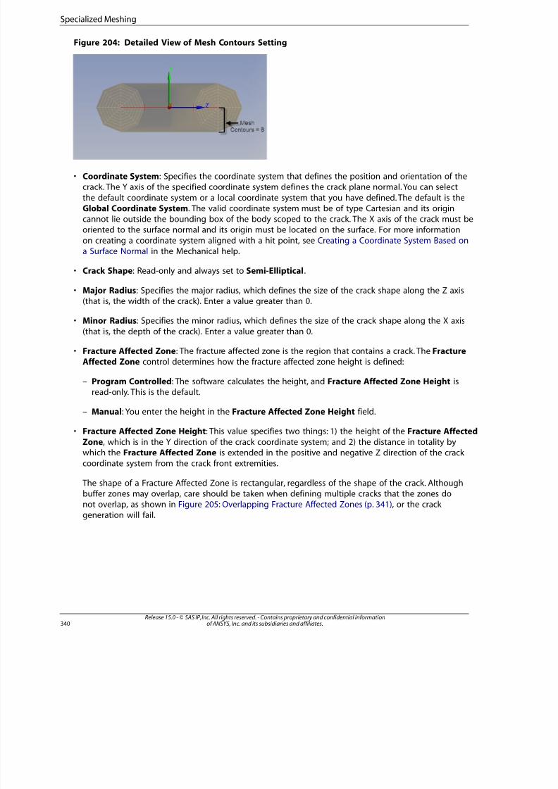
8/10/2019 ANSYS Meshing Users Guide
http://slidepdf.com/reader/full/ansys-meshing-users-guide 348/491
Figure 204: Detailed View of Mesh Contours Setting
• Coordinate System: Specifies the coordinate system that defines the position and orientation of thecrack. The Y axis of the specified coordinate system defines the crack plane normal. You can select
the default coordinate system or a local coordinate system that you have defined. The default is theGlobal Coordinate System. The valid coordinate system must be of type Cartesian and its origincannot lie outside the bounding box of the body scoped to the crack. The X axis of the crack must beoriented to the surface normal and its origin must be located on the surface. For more information
on creating a coordinate system aligned with a hit point, see Creating a Coordinate System Based on
a Surface Normal in the Mechanical help.
• Crack Shape: Read-only and always set to Semi-Elliptical .
• Major Radius: Specifies the major radius, which defines the size of the crack shape along the Z axis(that is, the width of the crack). Enter a value greater than 0.
• Minor Radius: Specifies the minor radius, which defines the size of the crack shape along the X axis
(that is, the depth of the crack). Enter a value greater than 0.
• Fracture Affected Zone: The fracture affected zone is the region that contains a crack. The FractureAffected Zone control determines how the fracture affected zone height is defined:
– Program Controlled: The software calculates the height, and Fracture Affected Zone Height isread-only. This is the default.
– Manual: You enter the height in the Fracture Affected Zone Height field.
• Fracture Affected Zone Height: This value specifies two things: 1) the height of the Fracture Affected
Zone, which is in the Y direction of the crack coordinate system; and 2) the distance in totality bywhich the Fracture Affected Zone is extended in the positive and negative Z direction of the crack coordinate system from the crack front extremities.
The shape of a Fracture Affected Zone is rectangular, regardless of the shape of the crack. Although
buffer zones may overlap, care should be taken when defining multiple cracks that the zones donot overlap, as shown in Figure 205: Overlapping Fracture Affected Zones (p. 341), or the crack generation will fail.
Release 15.0 - © SAS IP, Inc. All rights reserved. - Contains proprietary and confidential informationof ANSYS, Inc. and its subsidiaries and affiliates.340
Specialized Meshing
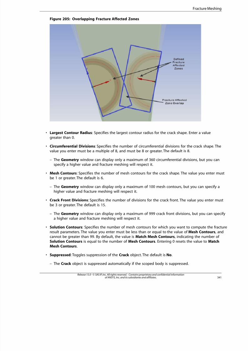
8/10/2019 ANSYS Meshing Users Guide
http://slidepdf.com/reader/full/ansys-meshing-users-guide 349/491
Figure 205: Overlapping Fracture Affected Zones
• Largest Contour Radius: Specifies the largest contour radius for the crack shape. Enter a value
greater than 0.
• Circumferential Divisions: Specifies the number of circumferential divisions for the crack shape. Thevalue you enter must be a multiple of 8, and must be 8 or greater. The default is 8.
– The Geometry window can display only a maximum of 360 circumferential divisions, but you can
specify a higher value and fracture meshing will respect it.
• Mesh Contours: Specifies the number of mesh contours for the crack shape. The value you enter mube 1 or greater. The default is 6.
– The Geometry window can display only a maximum of 100 mesh contours, but you can specify ahigher value and fracture meshing will respect it.
• Crack Front Divisions: Specifies the number of divisions for the crack front. The value you enter mus
be 3 or greater. The default is 15.
– The Geometry window can display only a maximum of 999 crack front divisions, but you can spec
a higher value and fracture meshing will respect it.
• Solution Contours: Specifies the number of mesh contours for which you want to compute the fractresult parameters. The value you enter must be less than or equal to the value of Mesh Contours, ancannot be greater than 99. By default, the value is Match Mesh Contours, indicating the number of Solution Contours is equal to the number of Mesh Contours. Entering 0 resets the value to Match
Mesh Contours.
• Suppressed: Toggles suppression of the Crack object. The default is No.
– The Crack object is suppressed automatically if the scoped body is suppressed.
34Release 15.0 - © SAS IP, Inc. All rights reserved. - Contains proprietary and confidential informationof ANSYS, Inc. and its subsidiaries and affiliates.
Fracture Meshing
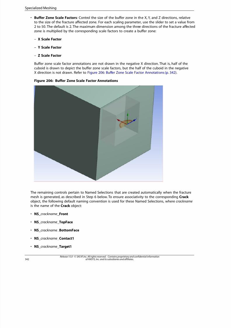
8/10/2019 ANSYS Meshing Users Guide
http://slidepdf.com/reader/full/ansys-meshing-users-guide 350/491
• Buffer Zone Scale Factors: Control the size of the buffer zone in the X, Y, and Z directions, relativeto the size of the fracture affected zone. For each scaling parameter, use the slider to set a value from
2 to 50. The default is 2. The maximum dimension among the three directions of the fracture affectedzone is multiplied by the corresponding scale factors to create a buffer zone:
– X Scale Factor
– Y Scale Factor
– Z Scale Factor
Buffer zone scale factor annotations are not drawn in the negative X direction. That is, half of the
cuboid is drawn to depict the buffer zone scale factors, but the half of the cuboid in the negativeX direction is not drawn. Refer to Figure 206: Buffer Zone Scale Factor Annotations (p. 342).
Figure 206: Buffer Zone Scale Factor Annotations
The remaining controls pertain to Named Selections that are created automatically when the fracturemesh is generated, as described in Step 6 below. To ensure associativity to the corresponding Crack object, the following default naming convention is used for these Named Selections, where crackname
is the name of the Crack object:
• NS_crackname_Front
• NS_crackname_TopFace
• NS_crackname_BottomFace
• NS_crackname_Contact1
• NS_crackname_Target1
Release 15.0 - © SAS IP, Inc. All rights reserved. - Contains proprietary and confidential informationof ANSYS, Inc. and its subsidiaries and affiliates.342
Specialized Meshing
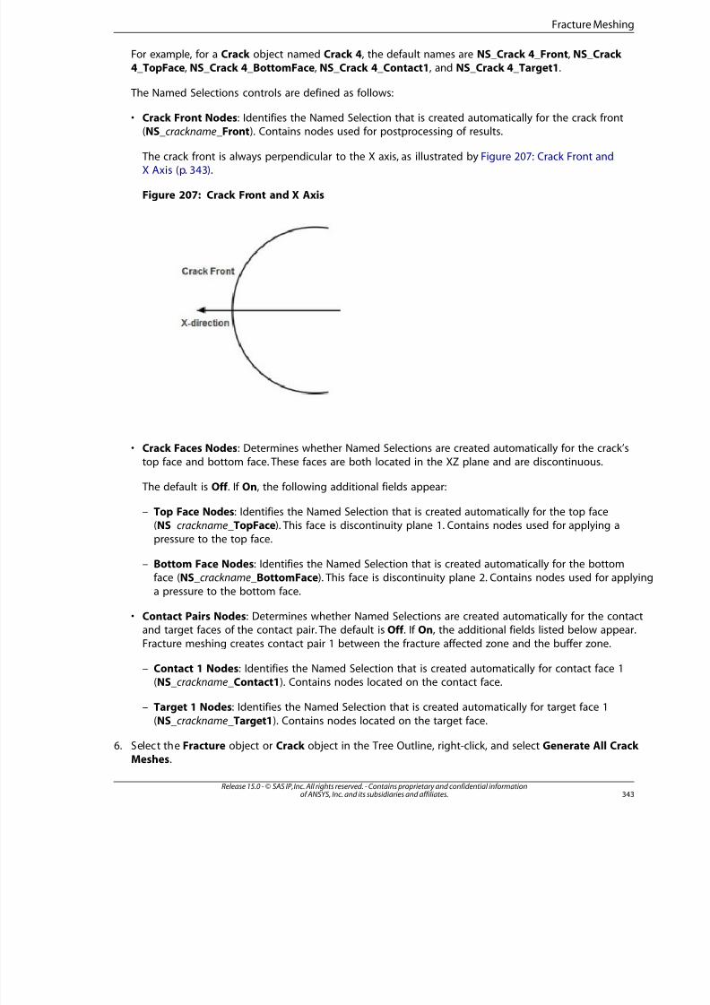
8/10/2019 ANSYS Meshing Users Guide
http://slidepdf.com/reader/full/ansys-meshing-users-guide 351/491
For example, for a Crack object named Crack 4, the default names are NS_Crack 4_Front, NS_Crack 4_TopFace, NS_Crack 4_BottomFace, NS_Crack 4_Contact1, and NS_Crack 4_Target1.
The Named Selections controls are defined as follows:
• Crack Front Nodes: Identifies the Named Selection that is created automatically for the crack front(NS_crackname_Front). Contains nodes used for postprocessing of results.
The crack front is always perpendicular to the X axis, as illustrated by Figure 207: Crack Front andX Axis (p. 343).
Figure 207: Crack Front and X Axis
• Crack Faces Nodes: Determines whether Named Selections are created automatically for the crack’s
top face and bottom face. These faces are both located in the XZ plane and are discontinuous.
The default is Off . If On, the following additional fields appear:
– Top Face Nodes: Identifies the Named Selection that is created automatically for the top face(NS_crackname_TopFace). This face is discontinuity plane 1. Contains nodes used for applying a
pressure to the top face.
– Bottom Face Nodes: Identifies the Named Selection that is created automatically for the bottomface (NS_crackname_BottomFace). This face is discontinuity plane 2. Contains nodes used for appl
a pressure to the bottom face.
• Contact Pairs Nodes: Determines whether Named Selections are created automatically for the conta
and target faces of the contact pair. The default is Off . If On, the additional fields listed below appearFracture meshing creates contact pair 1 between the fracture affected zone and the buffer zone.
– Contact 1 Nodes: Identifies the Named Selection that is created automatically for contact face 1(NS_crackname_Contact1). Contains nodes located on the contact face.
– Target 1 Nodes: Identifies the Named Selection that is created automatically for target face 1
(NS_crackname_Target1). Contains nodes located on the target face.
6. Select the Fracture object or Crack object in the Tree Outline, right-click, and select Generate All CracMeshes.
343Release 15.0 - © SAS IP, Inc. All rights reserved. - Contains proprietary and confidential informationof ANSYS, Inc. and its subsidiaries and affiliates.
Fracture Meshing

8/10/2019 ANSYS Meshing Users Guide
http://slidepdf.com/reader/full/ansys-meshing-users-guide 352/491
• When the fracture mesh is generated, the requested Named Selections are inserted into the TreeOutline under the Crack object with which they are associated.
• Click Show Mesh on the Graphics Options toolbar to display the fracture mesh.
Special Handling of Named Selections for Crack Objects
Crack objects dynamically generate Name Selections during fracture generation. The Named Selections
generated for Crack objects are a special type of Named Selection and have the following distinctproperties:
• Named Selections for Crack objects are not inserted into the Named Selections branch of the Tree Outline. They appear in the Tree Outline under the Crack object with which they are associated.
• You may rename a Named Selection by editing its name in the Details View of the Crack object or by
right-clicking the Named Selection in the Tree Outline and selecting Rename. Please use caution whenrenaming the Named Selection associated with the crack front (NS_crackname_Front). If the name is notunique when compared to other Named Selections, the crack definition sent to the solver may containthe wrong set of crack front nodes.
• You cannot insert, duplicate, copy, delete, or merge these Named Selections.
• You may scope nodal-based loads to these Named Selections.
• By default, nodal Named Selections show nodes attached to them in the Geometry window. To plot ele-
ments attached to these nodal Named Selections, refer to Specifying Annotation Preferences in theMechanical help.
• If you delete a Crack object, all associated Named Selections are deleted.
• If you suppress a Crack object, the nodal selection of each associated Named Selection is cleared and thestate of each Named Selections becomes suppressed.
• All Named Selections for Crack objects are sent to the solver. Send to Solver is always set to Yes and is
read-only.
• If Named Selections for Crack Faces Nodes and/or Contact Pairs Nodes have been created and yousubsequently set the fields to Off , the corresponding Named Selections are deleted when a new crack mesh is generated.
• For information about Named Selections in general, refer to Named Selections in the Mechanical help.
Note
For information about common fracture meshing problems and troubleshooting, see HandlingFracture Meshing Problems.
Release 15.0 - © SAS IP, Inc. All rights reserved. - Contains proprietary and confidential informationof ANSYS, Inc. and its subsidiaries and affiliates.344
Specialized Meshing
8/10/2019 ANSYS Meshing Users Guide
http://slidepdf.com/reader/full/ansys-meshing-users-guide 353/491
Meshing: Mesh Control Interaction Tables
This section presents the effects of applying combinations of mesh controls on the same part or body. Topics include the meshing implication when one mesh method is applied in combination with anothermesh method, and the effects of applying various mesh controls in combination with the various mesh
methods.Interactions Between Mesh MethodsInteractions Between Mesh Methods and Mesh Controls
Interactions Between Mesh Methods
The tables below present the effects of applying one mesh method in combination with another meshmethod, and include:
• Using combinations of surface mesh methods
• Using combinations of solid mesh methods
• Applying a single 3D inflation control on more than one solid body when a combination of mesh
methods has been scoped to the bodies
• Applying a 3D inflation control on a solid body when more than one mesh method has been scopedto the body
Note
• Assembly meshing algorithms cannot be used in combination with any other mesh method.
• Refer to Conformal Meshing Between Parts (p. 5) for information about conformal meshingand mesh method interoperability.
The table below describes the automatic sequencing of surface mesh methods when two mesh methodsare being used. If all three methods are being used, the automatic sequence is:
1. All Triangles
2. Quad Dominant
3. MultiZone Quad/Tri
Note
If you are performing selective meshing, you control the sequence. Refer to Selective Mesh-ing (p. 307) for usage notes.
345Release 15.0 - © SAS IP, Inc. All rights reserved. - Contains proprietary and confidential informationof ANSYS, Inc. and its subsidiaries and affiliates.
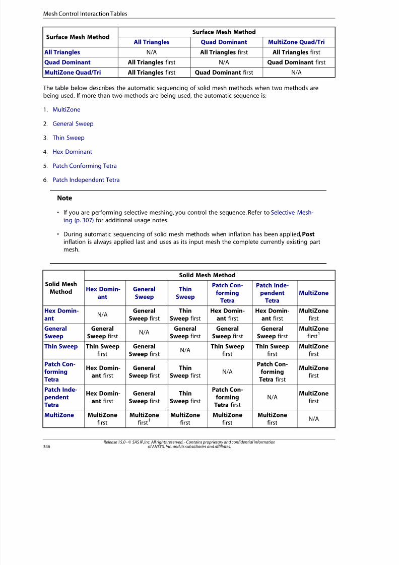
8/10/2019 ANSYS Meshing Users Guide
http://slidepdf.com/reader/full/ansys-meshing-users-guide 354/491
Surface Mesh MethodSurface Mesh Method
MultiZone Quad/TriQuad DominantAll Triangles
All Triangles firstAll Triangles firstN/AAll Triangles
Quad Dominant firstN/AAll Triangles firstQuad Dominant
N/AQuad Dominant firstAll Triangles firstMultiZone Quad/Tri
The table below describes the automatic sequencing of solid mesh methods when two methods arebeing used. If more than two methods are being used, the automatic sequence is:
1. MultiZone
2. General Sweep
3. Thin Sweep
4. Hex Dominant
5. Patch Conforming Tetra
6. Patch Independent Tetra
Note
• If you are performing selective meshing, you control the sequence. Refer to Selective Mesh-
ing (p. 307) for additional usage notes.
• During automatic sequencing of solid mesh methods when inflation has been applied, Postinflation is always applied last and uses as its input mesh the complete currently existing partmesh.
Solid Mesh Method
Solid MeshMethod MultiZone
Patch Inde-pendent
Tetra
Patch Con-forming
Tetra
Thin
Sweep
General
Sweep
Hex Domin-
ant
MultiZonefirst
Hex Domin-ant first
Hex Domin-ant first
ThinSweep first
GeneralSweep first
N/AHex Domin-ant
MultiZonefirst
1General
Sweep firstGeneral
Sweep firstGeneral
Sweep firstN/A
GeneralSweep first
GeneralSweep
MultiZone
first
Thin Sweep
first
Thin Sweep
firstN/A
General
Sweep first
Thin Sweep
first
Thin Sweep
MultiZonefirst
Patch Con-forming
Tetra firstN/A
ThinSweep first
GeneralSweep first
Hex Domin-ant first
Patch Con-formingTetra
MultiZone
firstN/A
Patch Con-forming
Tetra first
Thin
Sweep first
General
Sweep first
Hex Domin-
ant first
Patch Inde-pendentTetra
N/AMultiZone
firstMultiZone
firstMultiZone
firstMultiZone
first1
MultiZonefirst
MultiZone
Release 15.0 - © SAS IP, Inc. All rights reserved. - Contains proprietary and confidential informationof ANSYS, Inc. and its subsidiaries and affiliates.346
Mesh Control Interaction Tables
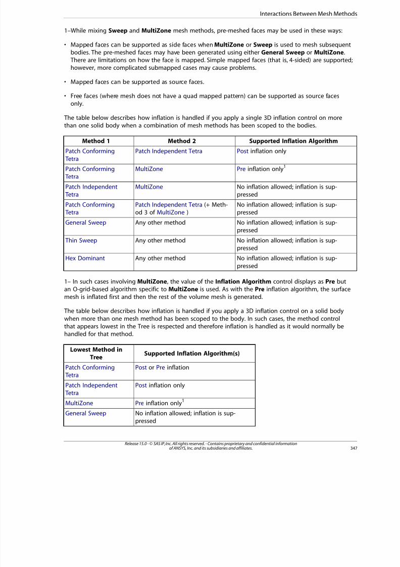
8/10/2019 ANSYS Meshing Users Guide
http://slidepdf.com/reader/full/ansys-meshing-users-guide 355/491
1–While mixing Sweep and MultiZone mesh methods, pre-meshed faces may be used in these ways:
• Mapped faces can be supported as side faces when MultiZone or Sweep is used to mesh subsequentbodies. The pre-meshed faces may have been generated using either General Sweep or MultiZone. There are limitations on how the face is mapped. Simple mapped faces (that is, 4-sided) are supported;however, more complicated submapped cases may cause problems.
• Mapped faces can be supported as source faces.
• Free faces (where mesh does not have a quad mapped pattern) can be supported as source facesonly.
The table below describes how inflation is handled if you apply a single 3D inflation control on morethan one solid body when a combination of mesh methods has been scoped to the bodies.
Supported Inflation AlgorithmMethod 2Method 1
Post inflation onlyPatch Independent TetraPatch Conforming
Tetra
Pre inflation only1
MultiZonePatch Conforming
TetraNo inflation allowed; inflation is sup-pressed
MultiZonePatch Independent Tetra
No inflation allowed; inflation is sup-pressed
Patch Independent Tetra (+ Meth-od 3 of MultiZone )
Patch Conforming Tetra
No inflation allowed; inflation is sup-pressed
Any other methodGeneral Sweep
No inflation allowed; inflation is sup-pressed
Any other method Thin Sweep
No inflation allowed; inflation is sup-
pressed
Any other methodHex Dominant
1– In such cases involving MultiZone, the value of the Inflation Algorithm control displays as Pre butan O-grid-based algorithm specific to MultiZone is used. As with the Pre inflation algorithm, the surfacemesh is inflated first and then the rest of the volume mesh is generated.
The table below describes how inflation is handled if you apply a 3D inflation control on a solid body
when more than one mesh method has been scoped to the body. In such cases, the method controlthat appears lowest in the Tree is respected and therefore inflation is handled as it would normally behandled for that method.
Supported Inflation Algorithm(s)
Lowest Method in
Tree
Post or Pre inflationPatch Conforming Tetra
Post inflation onlyPatch Independent Tetra
Pre inflation only1
MultiZone
No inflation allowed; inflation is sup-pressed
General Sweep
347Release 15.0 - © SAS IP, Inc. All rights reserved. - Contains proprietary and confidential informationof ANSYS, Inc. and its subsidiaries and affiliates.
Interactions Between Mesh Methods
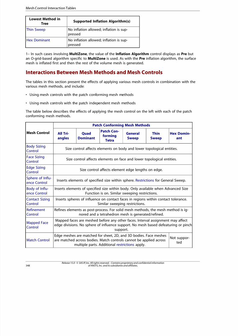
8/10/2019 ANSYS Meshing Users Guide
http://slidepdf.com/reader/full/ansys-meshing-users-guide 356/491
Supported Inflation Algorithm(s)Lowest Method in
Tree
No inflation allowed; inflation is sup-
pressed
Thin Sweep
No inflation allowed; inflation is sup-
pressed
Hex Dominant
1– In such cases involving MultiZone, the value of the Inflation Algorithm control displays as Pre butan O-grid-based algorithm specific to MultiZone is used. As with the Pre inflation algorithm, the surfacemesh is inflated first and then the rest of the volume mesh is generated.
Interactions Between Mesh Methods and Mesh Controls
The tables in this section present the effects of applying various mesh controls in combination with thevarious mesh methods, and include:
• Using mesh controls with the patch conforming mesh methods
• Using mesh controls with the patch independent mesh methods
The table below describes the effects of applying the mesh control on the left with each of the patchconforming mesh methods.
Patch Conforming Mesh Methods
Mesh Control Hex Domin-
ant
Thin
Sweep
General
Sweep
Patch Con-forming
Tetra
Quad
Dominant
All Tri-
angles
Size control affects elements on body and lower topological entities.Body SizingControl
Size control affects elements on face and lower topological entities.Face SizingControl
Size control affects element edge lengths on edge.Edge SizingControl
Inserts elements of specified size within sphere. Restrictions for General Sweep.Sphere of Influ-
ence Control
Inserts elements of specified size within body. Only available when Advanced Size
Function is on. Similar sweeping restrictions.
Body of Influ-
ence Control
Inserts spheres of influence on contact faces in regions within contact tolerance.Similar sweeping restrictions.
Contact SizingControl
Refines elements as post-process. For solid mesh methods, the mesh method is ig-nored and a tetrahedron mesh is generated/refined.
RefinementControl
Mapped faces are meshed before any other faces. Interval assignment may affectedge divisions. No sphere of influence support. No mesh based defeaturing or pinch
support.
Mapped FaceControl
Not suppor-ted
Edge meshes are matched for sheet, 2D, and 3D bodies. Face meshesare matched across bodies. Match controls cannot be applied across
multiple parts. Additional restrictions apply.
Match Control
Release 15.0 - © SAS IP, Inc. All rights reserved. - Contains proprietary and confidential informationof ANSYS, Inc. and its subsidiaries and affiliates.348
Mesh Control Interaction Tables
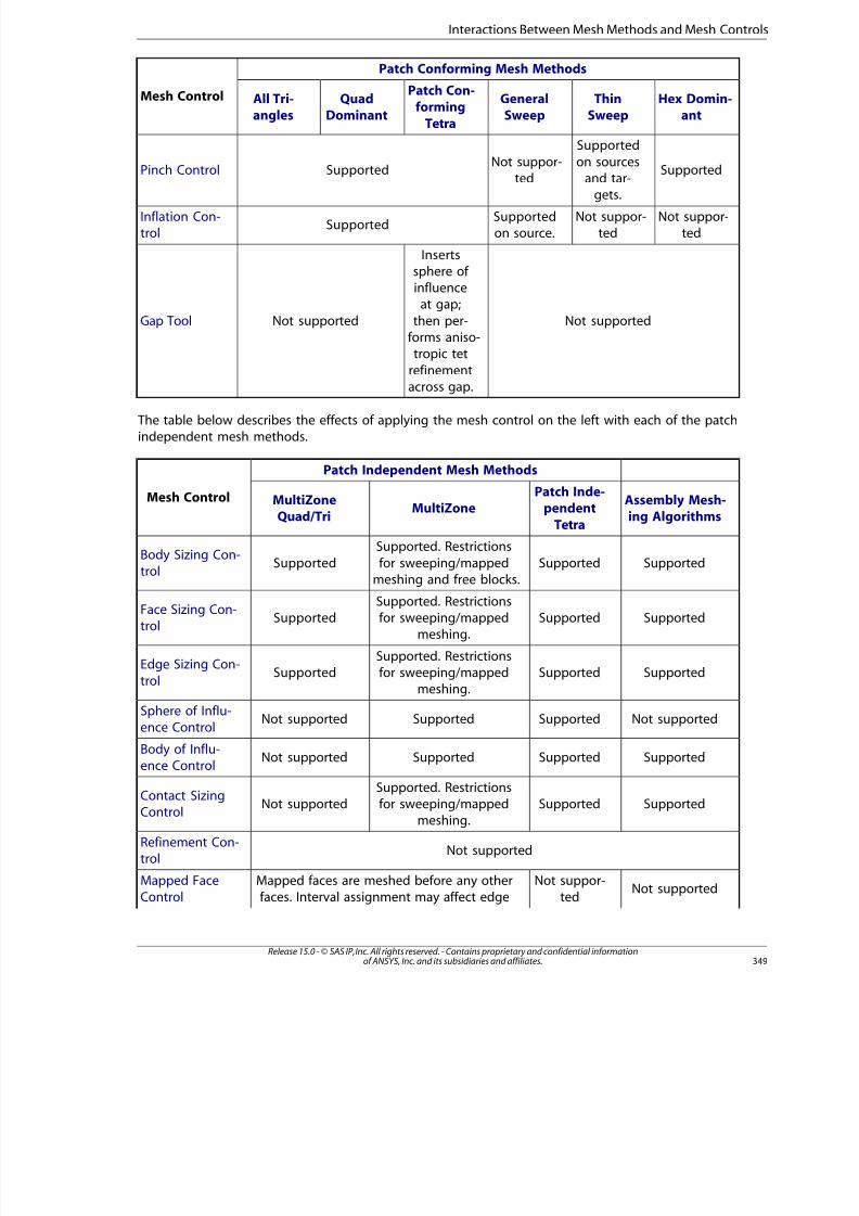
8/10/2019 ANSYS Meshing Users Guide
http://slidepdf.com/reader/full/ansys-meshing-users-guide 357/491
Patch Conforming Mesh Methods
Mesh Control Hex Domin-ant
ThinSweep
GeneralSweep
Patch Con-forming
Tetra
QuadDominant
All Tri-angles
Supported
Supported
on sourcesNot suppor-ted
SupportedPinch Controland tar-
gets.
Not suppor-ted
Not suppor-ted
Supportedon source.
SupportedInflation Con-trol
Not supported
Insertssphere of
Not supportedGap Tool
influenceat gap;
then per-forms aniso-tropic tet
refinement
across gap.
The table below describes the effects of applying the mesh control on the left with each of the patchindependent mesh methods.
Patch Independent Mesh Methods
Mesh Control Assembly Mesh-ing Algorithms
Patch Inde-pendent
Tetra
MultiZoneMultiZoneQuad/Tri
SupportedSupported
Supported. Restrictions
for sweeping/mappedmeshing and free blocks.
SupportedBody Sizing Con-
trol
SupportedSupportedSupported. Restrictionsfor sweeping/mapped
meshing.Supported
Face Sizing Con-trol
SupportedSupportedSupported. Restrictionsfor sweeping/mapped
meshing.Supported
Edge Sizing Con-
trol
Not supportedSupportedSupportedNot supportedSphere of Influ-ence Control
SupportedSupportedSupportedNot supported
Body of Influ-
ence Control
SupportedSupportedSupported. Restrictionsfor sweeping/mapped
meshing.Not supported
Contact SizingControl
Not supportedRefinement Con-trol
Not supportedNot suppor-
tedMapped faces are meshed before any otherfaces. Interval assignment may affect edge
Mapped FaceControl
349Release 15.0 - © SAS IP, Inc. All rights reserved. - Contains proprietary and confidential informationof ANSYS, Inc. and its subsidiaries and affiliates.
Interactions Between Mesh Methods and Mesh Controls

8/10/2019 ANSYS Meshing Users Guide
http://slidepdf.com/reader/full/ansys-meshing-users-guide 358/491
8/10/2019 ANSYS Meshing Users Guide
http://slidepdf.com/reader/full/ansys-meshing-users-guide 359/491
Meshing: Miscellaneous Tools
The miscellaneous meshing tools described in the following sections include:Generation of Contact ElementsRenaming Mesh Control Tool
Mesh NumberingMesh ConnectionCreating Section Planes
Passing Named Selections to the Solver
Generation of Contact Elements
To model contact between parts in an assembly, you must define specific contact conditions.
One of those conditions is tolerance, which controls the extent of contact between parts in an assembly. Tolerance is set as a percentage of the bounding box of the assembly. The bounding box is the smallestvolume that the assembly will fit in. You can change the tolerance (between -100 and 100) in the Options
dialog box under the Mechanical application's Connections category.
The higher the number, the tighter the tolerance. A loose tolerance generally increases the number of contact faces and areas of contact between parts, while a tight tolerance will decrease the number of contact faces.
Each face of the part is checked against the faces of other parts in the assembly. A contact pair is gen-erated between any faces within the tolerance. When solving, the elements for the two faces that make
up the pair are compared. If any of the faces are within the tolerance, contact elements are generatedfor them.
Note
This discussion is applicable to part-based meshing. The concept of an assembly of partsshould not be confused with assembly meshing. For assembly meshing, contact providesfeature capturing and contact sizing to close gaps; no contact elements or special interface
handling are involved.
Recommendations for Defining Contact for CFD Analyses
CFD users should be aware of the following recommendations:
• The Auto Detect Contact On Attach option controls whether contact detection is computed upongeometry import. If you do not want contact detection to be computed, make sure that it is disabled
by selecting Tools> Options from the ANSYS Workbench main menu, and then selecting either theMechanical or Meshing category as appropriate. The option is enabled by default in both applications.
• For CFX users, it is best practice to set the Group By option to None when defining Global ContactSettings. This is true because CFX only accepts contact pairs having a 1-to-1 correspondence. Setting
Group By to None ensures the 1-to-1 pairing needed for contact regions in these cases.
35Release 15.0 - © SAS IP, Inc. All rights reserved. - Contains proprietary and confidential informationof ANSYS, Inc. and its subsidiaries and affiliates.
8/10/2019 ANSYS Meshing Users Guide
http://slidepdf.com/reader/full/ansys-meshing-users-guide 360/491
• For ANSYS Fluent users, a boundary zone type of INTERFACE is assigned automatically to the contactsource and contact target entities that compose contact regions at the time of mesh export. See
Special Cases (p. 34) for details.
Renaming Mesh Control Tool
You can rename any of the mesh control tool objects to include the name assigned to the part or body. To do this, use a right mouse button click on the object and choose Rename Based on Definition fromthe context menu. For example, if you scope a Refinement tool to a body named Tube and chooseRename Based on Definition, the mesh control tool name changes from Refinement to Refinement
on Tube. The name change is reflected both in the tree and as a label on the body.
Mesh Numbering
The Mesh Numbering feature allows you to renumber the node and/or element numbers of a generatedmeshed model consisting of flexible parts. The feature is useful when exchanging or assembling modelsand could isolate the impact of using special elements such as superelements. For details, refer to MeshNumbering in the Mechanical help.
Mesh Connection
The Mesh Connection feature allows you to join the meshes of topologically disconnected surface
bodies that may reside in different parts. The connection can be edge-to-edge or edge-to-face. Themesh connection feature automatically generates post pinch controls internally at meshing time, allowingthe connections to work across parts so that a multibody part is not required. For details, refer to MeshConnection in the Mechanical help.
Creating Section Planes
For viewing purposes, you can use the Create Section Plane option to slice the graphical image of
your model based on a predefined coordinate system. For details, refer to Creating Section Planes inthe Mechanical help.
Passing Named Selections to the Solver
When defining Named Selections, you can use the Send to Solver option to control whether a NamedSelection is passed to the solver. Send to Solver is available in both the Mechanical and Meshing ap-plications.
The default is Yes for Named Selections that you create, and No for Named Selections that are generatedautomatically by the Mesh worksheet. When set to No, the selected Named Selection is not passed toANSYS Fluent, ANSYS CFX, Polyflow, CGNS, ANSYS ICEM CFD, ANSYS Fluent Meshing, Mechanical APDL,
ANSYS Autodyn, or any other downstream system that may be connected to the Mechanical or Meshingapplication.
Release 15.0 - © SAS IP, Inc. All rights reserved. - Contains proprietary and confidential informationof ANSYS, Inc. and its subsidiaries and affiliates.352
Miscellaneous Tools
8/10/2019 ANSYS Meshing Users Guide
http://slidepdf.com/reader/full/ansys-meshing-users-guide 361/491
Meshing: Ease of Use Features
The features described in this section are intended to assist you in meshing.Updating the Mesh Cell StateGenerating Mesh
Previewing Surface MeshPreviewing Source and Target MeshPreviewing Inflation
Showing Program Controlled Inflation SurfacesShowing Sweepable BodiesShowing Problematic GeometryShowing Geometry in Overlapping Named Selections
Showing Geometry in Overlapping Contact RegionsShowing Removable LoopsInspecting Large Meshes Using Named SelectionsGenerating Multiple Mesh Controls from a Template
Clearing Generated DataShowing Missing TessellationsShowing Mappable Faces
Updating the Mesh Cell State
In contrast to the Generate Mesh feature (which only produces the mesh), the Update feature determineswhether the geometry needs to be updated, refreshes the geometry if necessary, generates the mesh
if necessary, and also writes the output data for any connected cells:
• The Generate Mesh feature is useful when you are investigating the impact of different settings onthe mesh but you are not ready to export the mesh files.
• The Update feature is useful if you make a connection in the ANSYS Workbench Project Schematicfrom a Mesh cell to a system that requires a new type of output data (for example, if you make aconnection from the Mesh cell to a Fluid Flow (CFX) or Fluid Flow (Fluent) analysis system). In such
cases, the Mesh cell will go out-of-date. To bring the Mesh cell up-to-date, you can perform an Updateon the Mesh cell from within the Project Schematic, or follow the procedure below from within theMeshing application.
• If you connect a Mesh component system to an analysis system and the mesh file contains an assembly
mesh, the mesh file must be an ANSYS Fluent mesh file (*.msh) for it to be consumed by the down-stream system's solver. If the mesh file is of any other type, the Update fails and an error messageis issued.
• CFX does not support Assembly Mesh.
To update the Mesh cell:
1. Select the Mesh object or any mesh control object.
2. Right-click to display the context menu.
353Release 15.0 - © SAS IP, Inc. All rights reserved. - Contains proprietary and confidential informationof ANSYS, Inc. and its subsidiaries and affiliates.
8/10/2019 ANSYS Meshing Users Guide
http://slidepdf.com/reader/full/ansys-meshing-users-guide 362/491
3. Select Update in the menu.
Note
As an alternative to steps 2 and 3, you can click the Update button on the Mesh toolbar.
Generating Mesh
The Generate Mesh operation uses all defined meshing controls as input to generate a mesh. Generate
Mesh operates only on active objects, meaning that if bodies or controls are suppressed, they are ignoredby the meshing operation. You can generate mesh on the entire (active) model, or selectively on (active)parts and/or bodies. This includes single body parts, multibody parts, individual bodies, or multiple se-lected bodies across different parts or within the same part.
Note
• Selecting Generate Mesh generates a mesh based on the current mesh settings. It does notwrite the output data for any connected cells (downstream systems). Generate Mesh is useful
when you are investigating the impact of different settings on the mesh but you are not readyto export the mesh files. Refer to Updating the Mesh Cell State (p. 353) for related information.
• Using selective meshing, you can selectively pick bodies and mesh them incrementally. Aftermeshing a body, you can mesh the whole part or assembly or continue meshing individualbodies. Refer to Selective Meshing (p. 307) for additional information.
Suppressing and Unsuppressing Bodies in a Model
When there is a combination of suppressed and unsuppressed (active) bodies in a model, the Meshingapplication meshes only the active bodies. This is true regardless of mesh method. In addition, all influ-
ence of the suppressed bodies on neighboring bodies and their meshes is suppressed. For example, if a size control is applied to a suppressed body, the size control will not affect that body, nor will it influ-ence neighboring bodies (in general, if a size control is assigned to a suppressed body, that control isalso suppressed unless it is also attached to other active bodies). Refer to Selective Meshing (p. 307) for
additional information.
To generate the mesh for all active bodies:
1. Select the Mesh object or any mesh control object.
2. Right-click to display the context menu, or choose the Mesh drop down menu from the toolbar.
3. Select Generate Mesh in the menu. All active bodies are meshed. The mesh is displayed when youselect the Mesh object or the Show Mesh display option.
To generate the mesh for individual active bodies - from the object tree:
1. Select the Body objects.
2. Right-click to display the context menu.
3. Select Generate Mesh in the menu. The bodies are meshed. The meshes are displayed when you selectthe Mesh object or the Show Mesh display option.
Release 15.0 - © SAS IP, Inc. All rights reserved. - Contains proprietary and confidential informationof ANSYS, Inc. and its subsidiaries and affiliates.354
Ease of Use Features
8/10/2019 ANSYS Meshing Users Guide
http://slidepdf.com/reader/full/ansys-meshing-users-guide 363/491
To generate the mesh for individual active bodies - from the Geometry window:
1. Select the Mesh object.
2. Select the bodies in the Geometry window.
3. Right-click to display the context menu.
4. Select Generate Mesh On Selected Bodies in the menu. The bodies are meshed. The meshes are dis-played when you select the Mesh object in the tree or the Show Mesh display option.
To generate the mesh for individual active parts - from the object tree:
1. Select the Part objects.
2. Right-click to display the context menu.
3. Select Generate Mesh in the menu. The parts are meshed. The meshes are displayed when you selectthe Mesh object or the Show Mesh display option.
To generate the mesh for individual active parts - from the Geometry window:
1. Select the Mesh object.
2. Select the parts in the Geometry window.
3. Right-click to display the context menu.
4. Select Parts> Generate Mesh in the menu. The parts are meshed. The meshes are displayed when yoselect the Mesh object in the tree or the Show Mesh display option.
After successfully generating a mesh, you can view statistics about it. These statistics include meshmetric information that you can use to evaluate the mesh quality. For more information, see Statistics
Group (p. 121).
To re-mesh:
1. Select the Mesh object.
2. Right-click to display the context menu and select Clear Generated Data in the menu.
3. Confirm that you want to clear the mesh by clicking the Yes button.
4. Right-click on the Mesh object to display the context menu again and select Generate Mesh in themenu.
Note
• The order of topological entities is not guaranteed during a CAD source refresh. In cases inwhich you mesh, refresh, and re-mesh, the mesher may not produce exactly the same mesh if the refresh caused the topological entities to be reordered. As a result of this reordering, themesher meshes the entities in a different order as well, producing a slightly different result.
355Release 15.0 - © SAS IP, Inc. All rights reserved. - Contains proprietary and confidential informationof ANSYS, Inc. and its subsidiaries and affiliates.
Generating Mesh
8/10/2019 ANSYS Meshing Users Guide
http://slidepdf.com/reader/full/ansys-meshing-users-guide 364/491
• When selected from the Geometry object in the Tree Outline, the Generate Mesh RMB menuoption behaves slightly differently than when it is selected from the Mesh object in the Tree
Outline. Refer to Selective Meshing (p. 307) for details.
• Refer to "Meshing: Troubleshooting" (p. 391) for tips and strategies for handling problems thatmay occur during meshing.
Previewing Surface Mesh
You can preview the surface mesh for all unsuppressed parts, individual unsuppressed parts, or individualunsuppressed bodies. This includes single body parts, multibody parts, individual bodies, or multiple
selected bodies across different parts or within the same part. You can also export the previewed surfacemesh file in Fluent format, as described in Exporting a Previewed Surface Mesh in Fluent Format (p. 357).
Note
• This feature is not supported for the Patch Independent and MultiZone mesh method controls.
It is also not supported for thin model sweeping (that is, use of the Sweep mesh methodcontrol with Src/Trg Selection set to Manual Thin or Automatic Thin) or for assembly meshingalgorithms. (Refer to The Assembly Meshing Workflow (p. 276) for alternative approaches whenusing assembly meshing algorithms.)
• Influence of a swept body is an example of a size source that is fully integrated into the Ad-vanced Size Function, which means that it will contribute to the final mesh distribution obtainedby the mesher when the Advanced Size Function is on. However, the results obtained by eitherthe Preview Surface Mesh or Preview Inflation feature when the Advanced Size Function is
on may not accurately represent inflation layers and the surface mesh size distribution closeto a swept body when compared to the results obtained by the Generate Mesh feature, par-ticularly if there is bias along the sweep axis and/or the hex elements on the interface of the
inflation boundary are very thin.
• Refer to Selective Meshing (p. 307) for general information about selective meshing and limita-tions related to using the Preview Surface Mesh feature with selective meshing.
To preview the surface mesh for all unsuppressed parts:
1. Select the Mesh object or any mesh control object.
2. Right-click to display the context menu, or choose the Mesh drop down menu from the toolbar.
3. Select Preview> Surface Mesh in the context menu or Preview Surface Mesh in the drop down menu. The surface mesh is displayed for the model when you select the Mesh object.
To preview the surface mesh for individual unsuppressed parts - from the object tree:
1. Select the Part objects.
2. Right-click to display the context menu.
3. Select Preview> Surface Mesh in the menu. The surface mesh is displayed for the parts when you selectthe Mesh object.
Release 15.0 - © SAS IP, Inc. All rights reserved. - Contains proprietary and confidential informationof ANSYS, Inc. and its subsidiaries and affiliates.356
Ease of Use Features
8/10/2019 ANSYS Meshing Users Guide
http://slidepdf.com/reader/full/ansys-meshing-users-guide 365/491
To preview the surface mesh for individual unsuppressed parts - from the Geometry window:
1. Select the Mesh object.
2. Select the parts in the Geometry window.
3. Right-click to display the context menu.
4. Select Parts> Preview Surface Mesh in the menu. The surface mesh is displayed for the parts whenyou select the Mesh object in the tree.
To preview the surface mesh for individual unsuppressed bodies - from the object tree:
1. Select the Body objects.
2. Right-click to display the context menu.
3. Select Preview> Surface Mesh in the menu. The surface mesh is displayed for the bodies when youselect the Mesh object.
To preview the surface mesh for individual unsuppressed bodies - from the Geometry window:
1. Select the Mesh object.
2. Select the bodies in the Geometry window.
3. Right-click to display the context menu.
4. Select Preview Surface Mesh On Selected Bodies in the menu. The surface mesh is displayed for thebodies when you select the Mesh object in the tree.
After successfully previewing the surface mesh, you can view statistics about it. These statistics includemesh metric information that you can use to evaluate the mesh quality. For more information, see
Statistics Group (p. 121).
Exporting a Previewed Surface Mesh in Fluent Format
Follow the steps below to export a previewed surface mesh in Fluent format:
To export a previewed surface mesh in Fluent format:
1. Follow the procedure to preview a surface mesh.
2. Select File> Export from the main menu to export the surface mesh.
3. In the Save As dialog box, choose a directory and specify a file name for the file. Then choose FluentInput Files from the Save as type drop-down menu and click Save.
A .msh file suitable for import into Fluent will be created in the requested directory.
357Release 15.0 - © SAS IP, Inc. All rights reserved. - Contains proprietary and confidential informationof ANSYS, Inc. and its subsidiaries and affiliates.
Previewing Surface Mesh
8/10/2019 ANSYS Meshing Users Guide
http://slidepdf.com/reader/full/ansys-meshing-users-guide 366/491
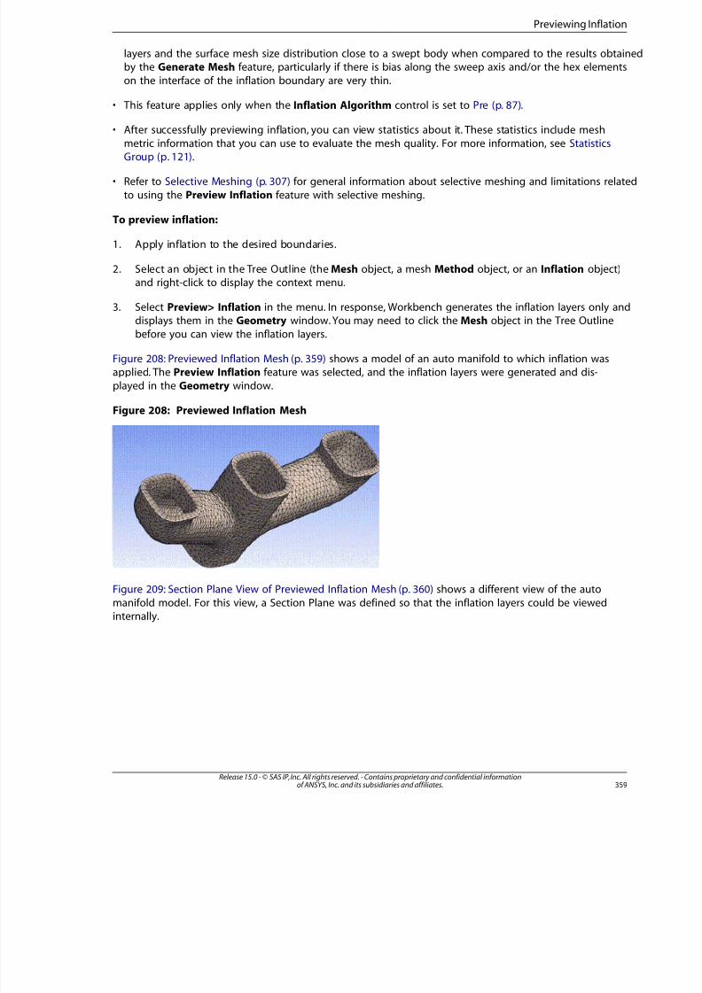
8/10/2019 ANSYS Meshing Users Guide
http://slidepdf.com/reader/full/ansys-meshing-users-guide 367/491
layers and the surface mesh size distribution close to a swept body when compared to the results obtaiby the Generate Mesh feature, particularly if there is bias along the sweep axis and/or the hex elements
on the interface of the inflation boundary are very thin.
• This feature applies only when the Inflation Algorithm control is set to Pre (p. 87).
• After successfully previewing inflation, you can view statistics about it. These statistics include mesh
metric information that you can use to evaluate the mesh quality. For more information, see Statistics
Group (p. 121).
• Refer to Selective Meshing (p. 307) for general information about selective meshing and limitations relat
to using the Preview Inflation feature with selective meshing.
To preview inflation:
1. Apply inflation to the desired boundaries.
2. Select an object in the Tree Outline (the Mesh object, a mesh Method object, or an Inflation object)and right-click to display the context menu.
3. Select Preview> Inflation in the menu. In response, Workbench generates the inflation layers only anddisplays them in the Geometry window. You may need to click the Mesh object in the Tree Outline
before you can view the inflation layers.
Figure 208: Previewed Inflation Mesh (p. 359) shows a model of an auto manifold to which inflation wasapplied. The Preview Inflation feature was selected, and the inflation layers were generated and dis-
played in the Geometry window.
Figure 208: Previewed Inflation Mesh
Figure 209: Section Plane View of Previewed Inflation Mesh (p. 360) shows a different view of the auto
manifold model. For this view, a Section Plane was defined so that the inflation layers could be viewedinternally.
359Release 15.0 - © SAS IP, Inc. All rights reserved. - Contains proprietary and confidential informationof ANSYS, Inc. and its subsidiaries and affiliates.
Previewing Inflation
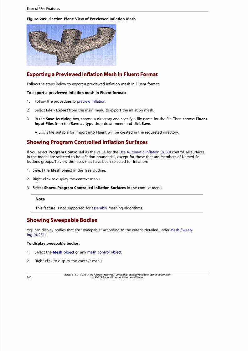
8/10/2019 ANSYS Meshing Users Guide
http://slidepdf.com/reader/full/ansys-meshing-users-guide 368/491
Figure 209: Section Plane View of Previewed Inflation Mesh
Exporting a Previewed Inflation Mesh in Fluent Format
Follow the steps below to export a previewed inflation mesh in Fluent format:
To export a previewed inflation mesh in Fluent format:
1. Follow the procedure to preview inflation.
2. Select File> Export from the main menu to export the inflation mesh.
3. In the Save As dialog box, choose a directory and specify a file name for the file. Then choose FluentInput Files from the Save as type drop-down menu and click Save.
A .msh file suitable for import into Fluent will be created in the requested directory.
Showing Program Controlled Inflation Surfaces
If you select Program Controlled as the value for the Use Automatic Inflation (p. 80) control, all surfacesin the model are selected to be inflation boundaries, except for those that are members of Named Se-
lections groups. To view the faces that have been selected for inflation:
1. Select the Mesh object in the Tree Outline.
2. Right-click to display the context menu.
3. Select Show> Program Controlled Inflation Surfaces in the context menu.
Note
This feature is not supported for assembly meshing algorithms.
Showing Sweepable BodiesYou can display bodies that are “sweepable” according to the criteria detailed under Mesh Sweep-ing (p. 231).
To display sweepable bodies:
1. Select the Mesh object or any mesh control object.
2. Right-click to display the context menu.
Release 15.0 - © SAS IP, Inc. All rights reserved. - Contains proprietary and confidential informationof ANSYS, Inc. and its subsidiaries and affiliates.360
Ease of Use Features

8/10/2019 ANSYS Meshing Users Guide
http://slidepdf.com/reader/full/ansys-meshing-users-guide 369/491
3. Select Show> Sweepable Bodies in the menu. All sweepable bodies are displayed.
Note
This feature is not supported for assembly meshing algorithms.
Showing Problematic Geometry
If problematic geometry causes meshing to fail, Workbench alerts you by:
• Displaying a Problematic Geometry message annotation in the Geometry window
• Displaying messages in the Messages window to describe the problem
For related information on viewing problematic geometry, refer to:
• Show Problematic Geometry in the DesignModeler help
• "Meshing: Troubleshooting" (p. 391)
Showing Geometry in Overlapping Named Selections
When the same entity is a member of more than one Named Selection, those Named Selections aresaid to be “overlapping.” If you are exporting a mesh into the ANSYS Fluent, Polyflow, CGNS, or ICEMCFD format (or faceted geometry for use in ANSYS Fluent Meshing), and overlapping Named Selections
are detected, the export fails and the Meshing application issues an error message to alert you to theoverlap problem. You must resolve the overlapping Named Selections before proceeding. To assist youin this task, you can display the geometry in the overlapping Named Selections in the Geometry window.
To display geometry in overlapping Named Selections:
1. Select the Mesh object.
2. Right-click to display the context menu.
3. Select Show> Geometry in Overlapping Named Selections in the menu. The overlapping geometryis highlighted in the Geometry window.
To proceed with the export, first resolve each of the overlapping Named Selections (for example, byremoving a duplicate entity from all but one of the overlapping Named Selections). After you resolve
each overlapping Named Selection, select Show> Geometry in Overlapping Named Selections andonly the remaining overlapping entities will be highlighted in the Geometry window. Once you haveresolved all of the overlapping Named Selections, the Show> Geometry in Overlapping Named Selec-
tions menu option will no longer appear in the menu and you can retry the export.
Showing Geometry in Overlapping Contact Regions
Contact regions are said to be “overlapping” when the same entity is a member of more than one
contact region or when multiple contact regions share the same geometry. ANSYS Fluent does notsupport overlapping contact regions. If you are exporting a mesh into the ANSYS Fluent format andoverlapping contact regions are detected, the export fails and the Meshing application issues an error
message to alert you to the overlap problem. You must resolve the overlapping contact regions before
36Release 15.0 - © SAS IP, Inc. All rights reserved. - Contains proprietary and confidential informationof ANSYS, Inc. and its subsidiaries and affiliates.
Showing Geometry in Overlapping Contact Regions
8/10/2019 ANSYS Meshing Users Guide
http://slidepdf.com/reader/full/ansys-meshing-users-guide 370/491
proceeding. For the case when the same entity is a member of more than one contact region, you candisplay the geometry in the overlapping contact regions in the Geometry window.
Note
This feature is applicable to part-based meshing only. The check for overlapping contact re-gions does not occur when assembly meshing algorithms are being used.
To display geometry in overlapping contact regions:
1. Select the Mesh object.
2. Right-click to display the context menu.
3. Select Show> Geometry in Overlapping Contact Regions in the menu. The overlapping geometry is
highlighted in the Geometry window.
To proceed with the export, first resolve each of the overlapping contact regions (for example, by re-moving a duplicate entity from all but one of the overlapping contact regions). After you resolve each
overlapping contact region, select Show> Geometry in Overlapping Contact Regions and only theremaining overlapping entities will be highlighted in the Geometry window. Once you have resolvedall of the overlapping contact regions, the Show> Geometry in Overlapping Contact Regions menuoption will no longer appear in the menu and you can retry the export.
Showing Removable Loops
You can use the Show Removable Loops feature prior to meshing to view loops that will be removedaccording to the criteria defined by the global Sheet Loop Removal and Loop Removal Tolerance
controls.
This feature applies only to sheet models, and it responds only to the settings of the global loop removal
controls. For example, if you set loop removal controls locally and your model contains loops that willbe removed according to your local criteria, the Show Removable Loops feature will return nothingif the global Sheet Loop Removal control is off (set to No).
To view removable loops:
1. Select the Mesh object in the Tree Outline.
2. Right-click to display the context menu.
3. Select Show> Removable Loops in the context menu.
Note
This feature is not supported for the MultiZone Quad/Tri mesh method or assembly meshingalgorithms.
Release 15.0 - © SAS IP, Inc. All rights reserved. - Contains proprietary and confidential informationof ANSYS, Inc. and its subsidiaries and affiliates.362
Ease of Use Features
8/10/2019 ANSYS Meshing Users Guide
http://slidepdf.com/reader/full/ansys-meshing-users-guide 371/491
Inspecting Large Meshes Using Named Selections
You can use Named Selections to inspect only a portion of the total mesh. Although this feature isavailable regardless of mesh size, it is most beneficial when working with a large mesh (greater than 5- 10 million nodes). For details, refer to Displaying Named Selections in the Mechanical help.
Generating Multiple Mesh Controls from a Template
The Object Generator enables you to make one or more copies of a template object, scoping each toa different piece of geometry. When defining mesh controls, you can use the Object Generator to make
copies of a template mesh control, which may reduce the necessity to manually define multiple relatedmesh controls. For details, refer to Generating Multiple Objects from a Template Object in the Mechan-ical help.
Clearing Generated Data
You can clear generated data from the database using a right-mouse click menu item. You can eitherclear all mesh and results data (if applicable) from a model, or clear the mesh data on the selected part
or body only.
Note
• When you clear the mesh, the status of the part or body will indicate that it is not meshed.
• When used on parts and bodies that have been joined by mesh connections or post pinch
controls, the Clear Generated Data option works as follows, where the "base" mesh, which isstored in a temporary file, is the mesh in its unsewn (pre-joined) state:
– If a base mesh is available, the mesh is reverted to the base mesh and the requested
parts/bodies are cleared.
– If no base mesh is available, the entire mesh is cleared and a warning message is issued.Reasons the base mesh may not be available include situations in which you have deletedyour temporary files, exported a .mechdat file for someone else to use, or moved your project
database to a different computer.
To clear all mesh and results data from a model - from the object tree:
1. Select the Mesh object in the Tree Outline.
2. Right-click to display the context menu.
3. Select Clear Generated Data in the context menu.
4. When asked whether you want to clear the data, click Yes.
To clear the mesh data from the selected part or body - from the object tree:
1. Select the part or body in the Tree Outline.
2. Right-click to display the context menu.
363Release 15.0 - © SAS IP, Inc. All rights reserved. - Contains proprietary and confidential informationof ANSYS, Inc. and its subsidiaries and affiliates.
Clearing Generated Data

8/10/2019 ANSYS Meshing Users Guide
http://slidepdf.com/reader/full/ansys-meshing-users-guide 372/491
3. Select Clear Generated Data in the context menu.
4. When asked whether you want to clear the mesh, click Yes.
To clear the mesh data from the selected body - from the Geometry window:
1. Select the Mesh object.
2. Select the bodies in the Geometry window.
3. Right-click to display the context menu.
4. Select Clear Generated Data On Selected Bodies in the context menu.
5. When asked whether you want to clear the mesh, click Yes.
To clear the mesh data from the selected part - from the Geometry window:
1. Select the Mesh object.
2. Select the part in the Geometry window.
3. Right-click to display the context menu.
4. Select Parts> Clear Generated Data in the context menu.
5. When asked whether you want to clear the mesh, click Yes.
Showing Missing Tessellations
Geometry with missing facets can lead to incorrect geometry representation by the mesher. Using the
Show Missing Tessellations feature, you can highlight geometry with missing facets, which will allowyou to detect and resolve problems prior to mesh generation.
Note
This feature is available only for the Patch Independent Tetra mesh method and assembly
meshing algorithms (both the CutCell and Tetrahedrons algorithms).
To highlight missing tessellations:
1. Select the Geometry object in the Tree Outline.
2. Right-click on the Geometry object or in the Geometry window to display the context menu.
3. Select Show Missing Tessellations in the context menu.
If a face without tessellations is found:
• The boundary of the face will be highlighted in the Geometry window.
• A warning message will be displayed in the Messages window advising you to use the Show Prob-lematic Geometry context menu option to locate the problem areas.
Release 15.0 - © SAS IP, Inc. All rights reserved. - Contains proprietary and confidential informationof ANSYS, Inc. and its subsidiaries and affiliates.364
Ease of Use Features

8/10/2019 ANSYS Meshing Users Guide
http://slidepdf.com/reader/full/ansys-meshing-users-guide 373/491
Showing Mappable Faces
You can display faces that are “mappable” according to the criteria detailed under Mapped FaceMeshing Control (p. 195).
To display mappable faces:
1. Select the Mesh object or any mesh control object.
2. Right-click to display the context menu.
3. Select Show> Mappable Faces in the menu. All mappable faces are highlighted in the Geometry
window.
4. Right-click on the Mesh object or mesh control object and select Insert> Mapped Face Meshing. Inthe Details View, the Geometry field shows the number of faces that are mappable and therefore wer
selected.
To edit the selected set of faces, click the Geometry field in the Details View to activate it. Then in theGeometry window, select the mappable faces that you want to use in the mapped face meshing control.
Click Apply in the Details View to complete your selection. Then proceed with the procedure describedin Mapped Face Meshing Control (p. 195).
Note
This feature is not supported for assembly meshing algorithms.
365Release 15.0 - © SAS IP, Inc. All rights reserved. - Contains proprietary and confidential informationof ANSYS, Inc. and its subsidiaries and affiliates.
Showing Mappable Faces

8/10/2019 ANSYS Meshing Users Guide
http://slidepdf.com/reader/full/ansys-meshing-users-guide 374/491
Release 15.0 - © SAS IP, Inc. All rights reserved. - Contains proprietary and confidential informationof ANSYS, Inc. and its subsidiaries and affiliates.366
8/10/2019 ANSYS Meshing Users Guide
http://slidepdf.com/reader/full/ansys-meshing-users-guide 375/491
Meshing: Virtual Topology
Uses of virtual topology include:
• Before performing analysis of a CAD model, you may want to group faces/edges together to form virtua
cells. In such cases, virtual topology can aid you in reducing the number of elements in the model, simpfying small features out of the model, and simplifying load abstraction.
• You can split a face to create two virtual faces, or split an edge to create two virtual edges. For example,in the case of a rectangular face in which a single edge on one side of the face corresponds to two edge
on the opposite side of the face, you can split the single edge so that node alignment across the face cahave similar spacing.
• When needed, you can create virtual hard vertices to facilitate split face operations.
• Virtual topology can be helpful for handling fillets for MultiZone and sweep meshing. See Using Virtual Topology to Handle Fillets in MultiZone Problems (p. 269).
The following sections cover these topics:
IntroductionCreating and Managing Virtual CellsCreating and Managing Virtual Split EdgesCreating and Managing Virtual Split Faces
Creating and Managing Virtual Hard VerticesCommon Virtual Topology OperationsCommon Virtual Topology Features
Introduction
A CAD Model has two parts:
1. Topology: The connectivity of a CAD model, meaning: vertices are connected to edges, which are
connected to faces, which are connected to volumes. Each one of these entities is referred to as acell.
2. Geometry: The geometry of the CAD model is the underlying mathematical definition of the
aforementioned cells.
A virtual cell in the Mechanical application or the Meshing application modifies the topology of onlythe local copy in the Mechanical application or Meshing application. Your original CAD model remainsunchanged. New faceted geometry is also created with virtual topology. However, the mesher may
project the nodes back to the original geometry where applicable.
For information about the virtual topology operations that you can perform, refer to:
• Creating and Managing Virtual Cells (p. 368)
• Creating and Managing Virtual Split Edges (p. 374)
367Release 15.0 - © SAS IP, Inc. All rights reserved. - Contains proprietary and confidential informationof ANSYS, Inc. and its subsidiaries and affiliates.

8/10/2019 ANSYS Meshing Users Guide
http://slidepdf.com/reader/full/ansys-meshing-users-guide 376/491
• Creating and Managing Virtual Split Faces (p. 378)
• Creating and Managing Virtual Hard Vertices (p. 381)
• Common Virtual Topology Operations (p. 381)
• Common Virtual Topology Features (p. 385)
Creating and Managing Virtual CellsYou can manually designate faces and edges for inclusion into a virtual cell, or you can have theMechanical application or the Meshing application automatically create virtual cells based on settings
that you specify. The geometry under a virtual cell is represented by the underlying cell's graphic resol-ution.
Note
• There are geometric limitations to creating virtual cells, including those related to cells thatwould have too much curvature, or other limitations in trying to represent a group of cells by
a single cell.
• The tessellation of models from CATIA4 may not be appropriate for virtual topology, whichcould prevent the creation of virtual cells for these models.
Creating Virtual Cells Manually
1. Insert a Virtual Topology object in the tree.
2. Choose the face or edge selection filter, and then pick one or more faces or one or more edges that youwant to include in the virtual cell(s).
3. Create the Virtual Cell object(s) by doing one of the following:
• Choose Merge Cells on the Virtual Topology context toolbar.
• Click right mouse button on the Virtual Topology object and select Insert> Virtual Cell from thecontext menu.
• Click right mouse button in the Geometry window and select Insert> Virtual Cell from the contextmenu.
From the selected set of faces or edges, the software creates the virtual cell(s). During this process,
adjacent selected entities are grouped appropriately to form virtual cell(s), while any single selectedentity (that is, one that is selected but is not adjacent to any other selected entity) forms its ownvirtual cell. An error message appears in the Messages window for each subset of failed topologies. To highlight the geometry that is responsible for a message, select the message, right-click, and
select Show Problematic Geometry from the context menu. Refer to the examples below.
Note
• A virtual cell cannot be created on a single edge that is straight or enclosed with no vertices.
Release 15.0 - © SAS IP, Inc. All rights reserved. - Contains proprietary and confidential informationof ANSYS, Inc. and its subsidiaries and affiliates.368
Virtual Topology
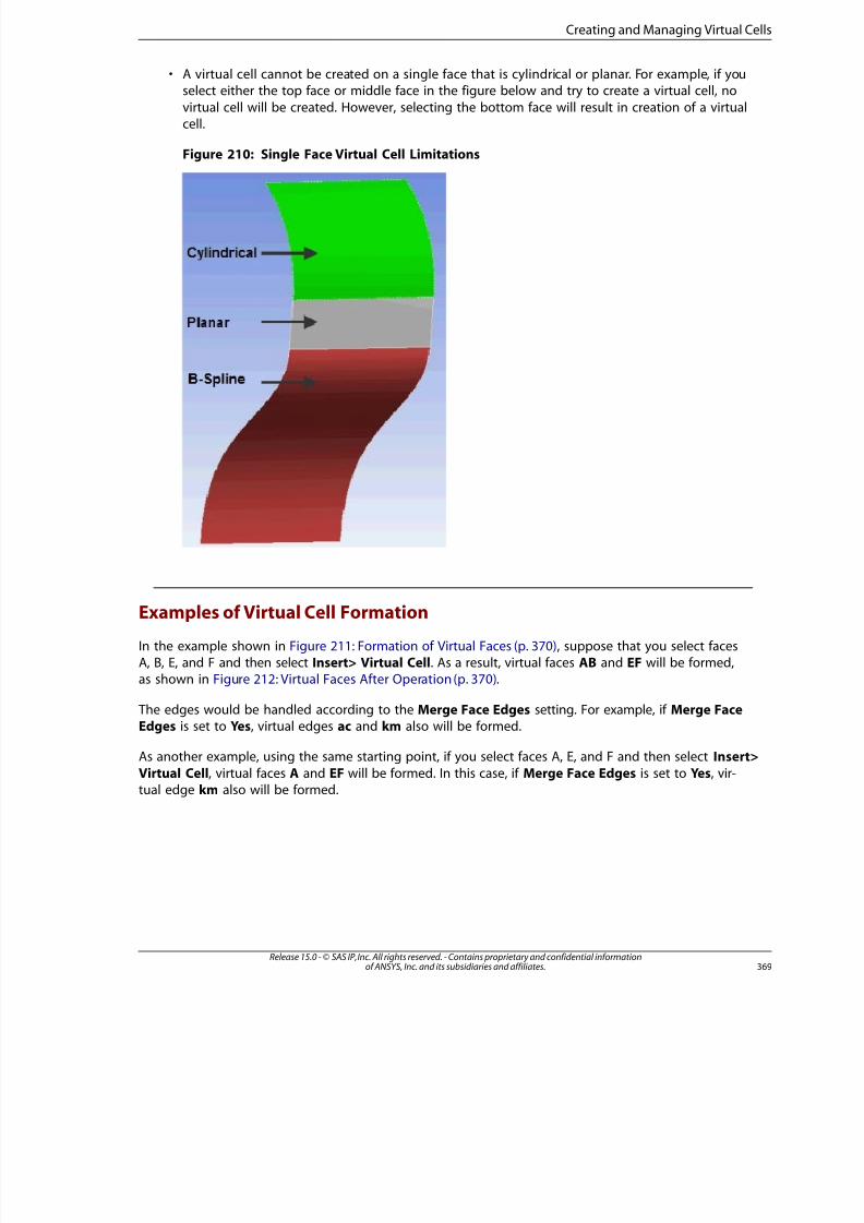
8/10/2019 ANSYS Meshing Users Guide
http://slidepdf.com/reader/full/ansys-meshing-users-guide 377/491
• A virtual cell cannot be created on a single face that is cylindrical or planar. For example, if youselect either the top face or middle face in the figure below and try to create a virtual cell, no
virtual cell will be created. However, selecting the bottom face will result in creation of a virtualcell.
Figure 210: Single Face Virtual Cell Limitations
Examples of Virtual Cell Formation
In the example shown in Figure 211: Formation of Virtual Faces (p. 370), suppose that you select facesA, B, E, and F and then select Insert> Virtual Cell. As a result, virtual faces AB and EF will be formed,as shown in Figure 212: Virtual Faces After Operation (p. 370).
The edges would be handled according to the Merge Face Edges setting. For example, if Merge FaceEdges is set to Yes, virtual edges ac and km also will be formed.
As another example, using the same starting point, if you select faces A, E, and F and then select Insert>
Virtual Cell, virtual faces A and EF will be formed. In this case, if Merge Face Edges is set to Yes, vir-tual edge km also will be formed.
369Release 15.0 - © SAS IP, Inc. All rights reserved. - Contains proprietary and confidential informationof ANSYS, Inc. and its subsidiaries and affiliates.
Creating and Managing Virtual Cells
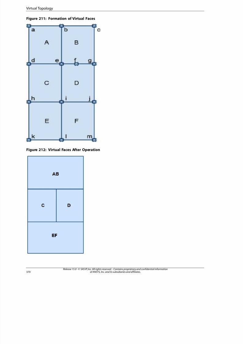
8/10/2019 ANSYS Meshing Users Guide
http://slidepdf.com/reader/full/ansys-meshing-users-guide 378/491
Figure 211: Formation of Virtual Faces
Figure 212: Virtual Faces After Operation
Release 15.0 - © SAS IP, Inc. All rights reserved. - Contains proprietary and confidential informationof ANSYS, Inc. and its subsidiaries and affiliates.370
Virtual Topology
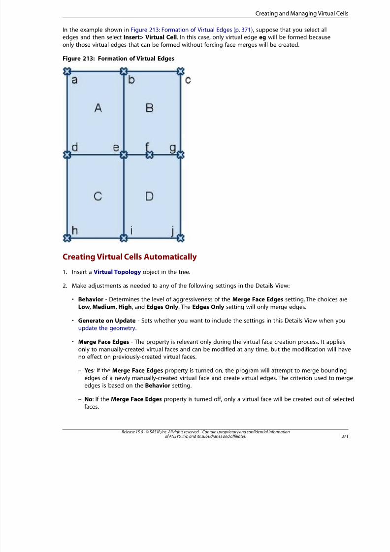
8/10/2019 ANSYS Meshing Users Guide
http://slidepdf.com/reader/full/ansys-meshing-users-guide 379/491
In the example shown in Figure 213: Formation of Virtual Edges (p. 371), suppose that you select alledges and then select Insert> Virtual Cell. In this case, only virtual edge eg will be formed because
only those virtual edges that can be formed without forcing face merges will be created.
Figure 213: Formation of Virtual Edges
Creating Virtual Cells Automatically1. Insert a Virtual Topology object in the tree.
2. Make adjustments as needed to any of the following settings in the Details View:
• Behavior - Determines the level of aggressiveness of the Merge Face Edges setting. The choices are
Low, Medium, High, and Edges Only. The Edges Only setting will only merge edges.
• Generate on Update - Sets whether you want to include the settings in this Details View when youupdate the geometry.
• Merge Face Edges - The property is relevant only during the virtual face creation process. It appliesonly to manually-created virtual faces and can be modified at any time, but the modification will havno effect on previously-created virtual faces.
– Yes: If the Merge Face Edges property is turned on, the program will attempt to merge bounding
edges of a newly manually-created virtual face and create virtual edges. The criterion used to mergedges is based on the Behavior setting.
– No: If the Merge Face Edges property is turned off, only a virtual face will be created out of select
faces.
37Release 15.0 - © SAS IP, Inc. All rights reserved. - Contains proprietary and confidential informationof ANSYS, Inc. and its subsidiaries and affiliates.
Creating and Managing Virtual Cells

8/10/2019 ANSYS Meshing Users Guide
http://slidepdf.com/reader/full/ansys-meshing-users-guide 380/491
• Lock position of dependent edge splits - See Locking Locations of Dependent Virtual SplitEdges (p. 376).
• Virtual Faces, Virtual Edges, Virtual Split Edges, Virtual Split Faces, Virtual Hard Vertices, TotalVirtual Entities - Read-only indications of corresponding counts in the model. See Viewing Virtual Topology Statistics (p. 388).
3. Do one of the following:
• Click right mouse button on the Virtual Topology object and choose Generate Virtual Cells fromthe context menu. Virtual cells are automatically created for each region that meets the criteria estab-
lished by the settings in step 2.
These virtual cells remain valid after a geometry update.
• Choose the face or body selection filter and pick two or more faces or two or more bodies. Click right
mouse button on the Virtual Topology object and choose Generate Virtual Cells on Selected Entitiesfrom the context menu. From the selected set of faces or bodies, the software groups adjacent entitiesappropriately and automatically creates virtual cells for each region that meets the criteria establishedby the settings in step 2.
These virtual cells become invalid after a geometry update.
Notes on Virtual Cell Creation
• Scoped objects except other virtual cells may need to be relinked to the new virtual cells when that virtualcell is comprised of entities in the scoped object. When the virtual cell is deleted the object may need tobe rescoped to the original entities.
• All scoped objects except for mesh controls and other virtual cells will be protected during automaticvirtual cell generation. This will allow users to load their models and run auto virtual topology withoutdeleting loads. All faces within a protected object may be merged with faces in the same protected object
and not in any other protected object.
• If Generate on Update is set to Yes and you update the geometry, all Virtual Cell objects that werecreated automatically will be deleted and recreated based on the new geometry. Any loads that were at-tached to geometry within the deleted Virtual Cell objects will need to be reattached to the new geometry.
• If Generate on Update is set to No and you update the geometry, all Virtual Cell objects that were createdautomatically should remain persistent barring major topology changes of the model being updated.Reapplication of loads may not be necessary.
• For any virtual cells that were generated, you can choose whether the nodes will be projected back tothe underlying geometry (in contrast to the virtual cell’s faceted geometry). To do so, select the desired
virtual cell and use the Virtual Topology Properties dialog to set the Project to Underlying Geometryoption to Yes or No. The default is Yes for analytical geometry; otherwise, the default is No. Computational
expense increases when the option is set to Yes. Use these guidelines:
– Yes is recommended if:
You are using virtual topology to fine tune the topology of your mesh and need precise control from
the Advanced Size Function.
Release 15.0 - © SAS IP, Inc. All rights reserved. - Contains proprietary and confidential informationof ANSYS, Inc. and its subsidiaries and affiliates.372
Virtual Topology
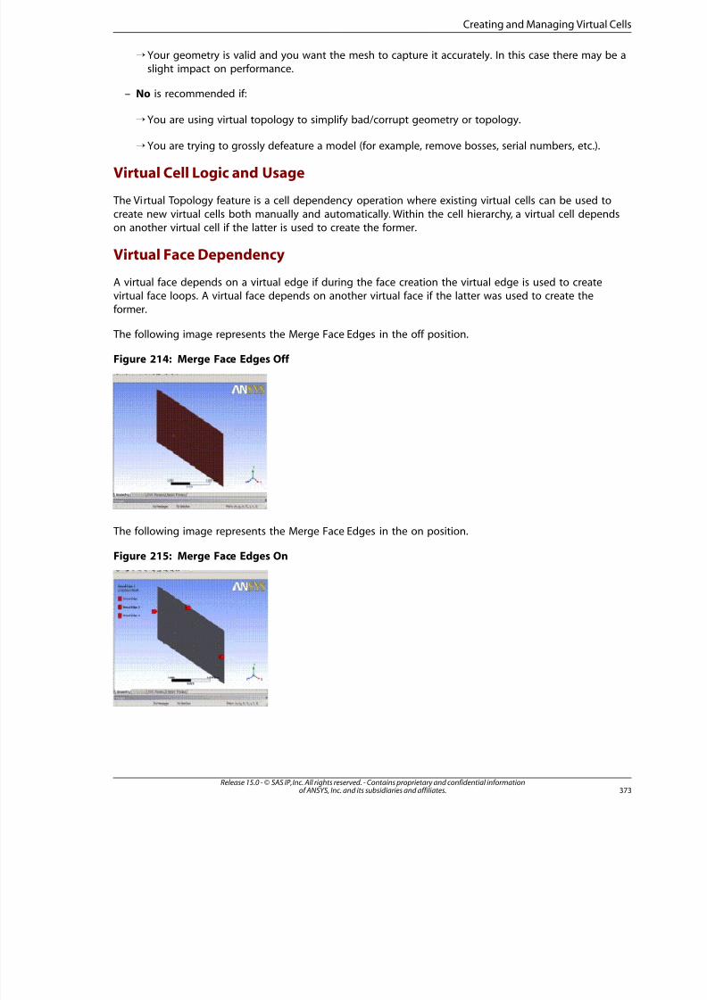
8/10/2019 ANSYS Meshing Users Guide
http://slidepdf.com/reader/full/ansys-meshing-users-guide 381/491
Your geometry is valid and you want the mesh to capture it accurately. In this case there may be aslight impact on performance.
– No is recommended if:
You are using virtual topology to simplify bad/corrupt geometry or topology.
You are trying to grossly defeature a model (for example, remove bosses, serial numbers, etc.).
Virtual Cell Logic and Usage
The Virtual Topology feature is a cell dependency operation where existing virtual cells can be used to
create new virtual cells both manually and automatically. Within the cell hierarchy, a virtual cell dependson another virtual cell if the latter is used to create the former.
Virtual Face Dependency
A virtual face depends on a virtual edge if during the face creation the virtual edge is used to createvirtual face loops. A virtual face depends on another virtual face if the latter was used to create the
former.
The following image represents the Merge Face Edges in the off position.
Figure 214: Merge Face Edges Off
The following image represents the Merge Face Edges in the on position.
Figure 215: Merge Face Edges On
373Release 15.0 - © SAS IP, Inc. All rights reserved. - Contains proprietary and confidential informationof ANSYS, Inc. and its subsidiaries and affiliates.
Creating and Managing Virtual Cells
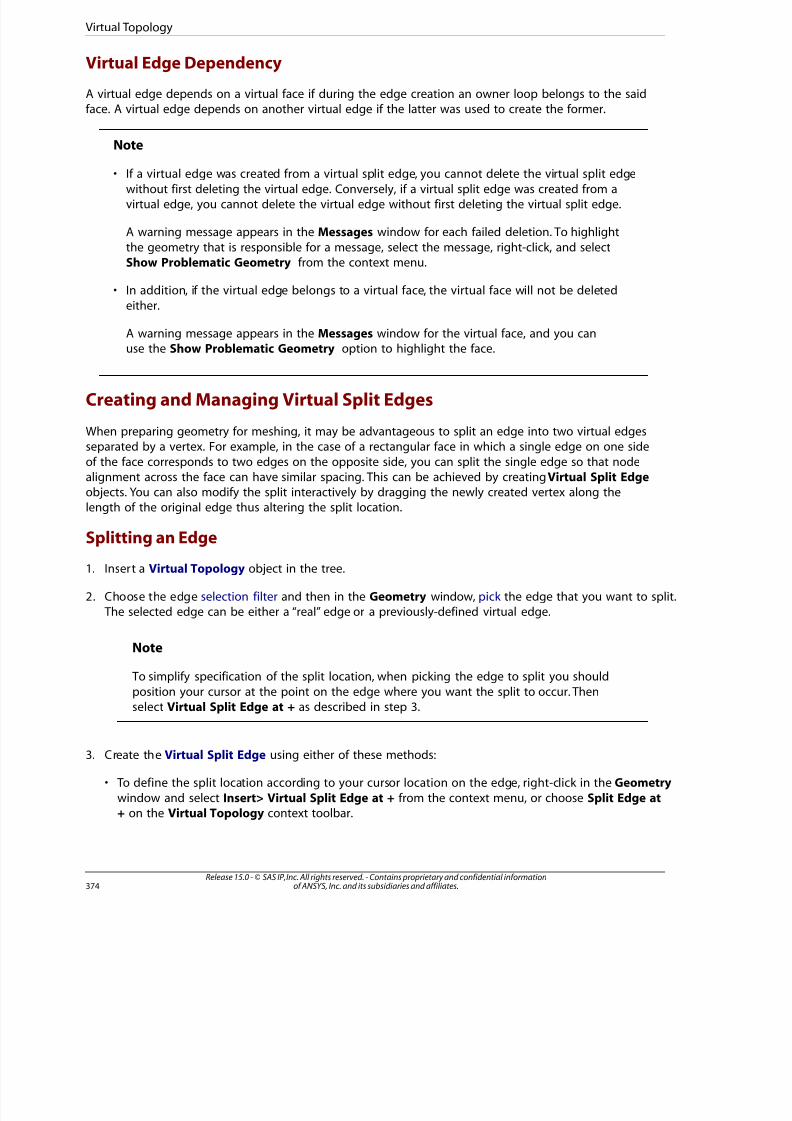
8/10/2019 ANSYS Meshing Users Guide
http://slidepdf.com/reader/full/ansys-meshing-users-guide 382/491
Virtual Edge Dependency
A virtual edge depends on a virtual face if during the edge creation an owner loop belongs to the saidface. A virtual edge depends on another virtual edge if the latter was used to create the former.
Note
• If a virtual edge was created from a virtual split edge, you cannot delete the virtual split edgewithout first deleting the virtual edge. Conversely, if a virtual split edge was created from avirtual edge, you cannot delete the virtual edge without first deleting the virtual split edge.
A warning message appears in the Messages window for each failed deletion. To highlight
the geometry that is responsible for a message, select the message, right-click, and selectShow Problematic Geometry from the context menu.
• In addition, if the virtual edge belongs to a virtual face, the virtual face will not be deleted
either.
A warning message appears in the Messages window for the virtual face, and you can
use the Show Problematic Geometry option to highlight the face.
Creating and Managing Virtual Split Edges
When preparing geometry for meshing, it may be advantageous to split an edge into two virtual edgesseparated by a vertex. For example, in the case of a rectangular face in which a single edge on one side
of the face corresponds to two edges on the opposite side, you can split the single edge so that nodealignment across the face can have similar spacing. This can be achieved by creating Virtual Split Edgeobjects. You can also modify the split interactively by dragging the newly created vertex along thelength of the original edge thus altering the split location.
Splitting an Edge
1. Insert a Virtual Topology object in the tree.
2. Choose the edge selection filter and then in the Geometry window, pick the edge that you want to split. The selected edge can be either a “real” edge or a previously-defined virtual edge.
Note
To simplify specification of the split location, when picking the edge to split you should
position your cursor at the point on the edge where you want the split to occur. Then
select Virtual Split Edge at + as described in step 3.
3. Create the Virtual Split Edge using either of these methods:
• To define the split location according to your cursor location on the edge, right-click in the Geometry
window and select Insert> Virtual Split Edge at + from the context menu, or choose Split Edge at+ on the Virtual Topology context toolbar.
Release 15.0 - © SAS IP, Inc. All rights reserved. - Contains proprietary and confidential informationof ANSYS, Inc. and its subsidiaries and affiliates.374
Virtual Topology
8/10/2019 ANSYS Meshing Users Guide
http://slidepdf.com/reader/full/ansys-meshing-users-guide 383/491
• To define the split without specifying the location, select the edge you want to split, right-click in theGeometry window, and select Insert> Virtual Split Edge from the context menu, or choose Split
Edge on the Virtual Topology context toolbar. By default the split ratio will be set to 0.5, but youcan change it later by using the Virtual Topology Properties dialog.
Note
If the software cannot create the split, the error message “Unable to split the edge atselected location or with given split ratio” will appear and the split will not be created.
4. In step 3, if you created the Virtual Split Edge object by selecting Virtual Split Edge at +, the split ratis determined automatically by the software. If you created it by selecting Virtual Split Edge, you caneither accept the default of 0.5 or specify a different split ratio by right-clicking and selecting Edit Sele
Virtual Entity Properties.... Then edit the Split Ratio field on the Virtual Topology Properties dialog
The split ratio defines the location of the split by specifying the ratio between the distance fromthe start point of the edge to the split location and the overall length of the edge. Specify a value
from 0 to 1. For example, a value of 0.5 will split the edge into two edges of equal length. A value
of 0.75 will split the edge into two edges where the first edge is three quarters of the length of theoriginal edge, and the second edge is only one quarter of the length of the original edge. A valueof 0 or 1 is valid only if the selected edge is a closed edge. In the case of a closed edge, such as a
circle, the edge will be split into two edges, and the new vertex will be placed along one of thenew edges.
You can change the location of the split at any time by accessing the Virtual Topology Properties
dialog and editing the Split Ratio field, or by modifying the edge split interactively.
To modify an edge split interactively, select any portion of the original edge or its vertex split locationin the Geometry view. Then, while pressing F4 on the keyboard, drag the mouse along the lengthof the edge to redistribute the split ratio. The display indicates the initial 3-D location of the split,
together with a preview of its new location and split ratio.
When you change the split ratio of an edge split that is attached to a face split, both the edge splitand the face split are adjusted accordingly.
Virtual Split Edge Dependency
Existing virtual edges and/or existing virtual split edges can be used to create new virtual split edges.
Within the split edge hierarchy, a virtual split edge depends on a virtual edge if the latter is used tocreate the former. Similarly, a virtual split edge depends on another virtual split edge if the latter isused to create the former.
Note
If a virtual edge was created from a virtual split edge, you cannot delete the virtual split edgewithout first deleting the virtual edge. Conversely, if a virtual split edge was created from avirtual edge, you cannot delete the virtual edge without first deleting the virtual split edge.
A warning message appears in the Messages window for each failed deletion. To highlight
the geometry that is responsible for a message, select the message, right-click, and selectShow Problematic Geometry from the context menu.
375Release 15.0 - © SAS IP, Inc. All rights reserved. - Contains proprietary and confidential informationof ANSYS, Inc. and its subsidiaries and affiliates.
Creating and Managing Virtual Split Edges
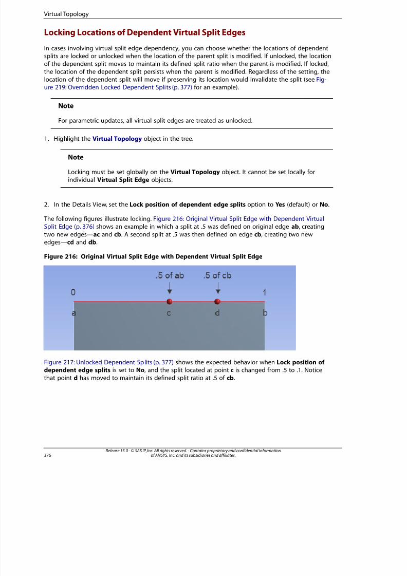
8/10/2019 ANSYS Meshing Users Guide
http://slidepdf.com/reader/full/ansys-meshing-users-guide 384/491
Locking Locations of Dependent Virtual Split Edges
In cases involving virtual split edge dependency, you can choose whether the locations of dependentsplits are locked or unlocked when the location of the parent split is modified. If unlocked, the locationof the dependent split moves to maintain its defined split ratio when the parent is modified. If locked,
the location of the dependent split persists when the parent is modified. Regardless of the setting, thelocation of the dependent split will move if preserving its location would invalidate the split (see Fig-
ure 219: Overridden Locked Dependent Splits (p. 377) for an example).
Note
For parametric updates, all virtual split edges are treated as unlocked.
1. Highlight the Virtual Topology object in the tree.
Note
Locking must be set globally on the Virtual Topology object. It cannot be set locally for
individual Virtual Split Edge objects.
2. In the Details View, set the Lock position of dependent edge splits option to Yes (default) or No.
The following figures illustrate locking. Figure 216: Original Virtual Split Edge with Dependent VirtualSplit Edge (p. 376) shows an example in which a split at .5 was defined on original edge ab, creating
two new edges—ac and cb. A second split at .5 was then defined on edge cb, creating two newedges—cd and db.
Figure 216: Original Virtual Split Edge with Dependent Virtual Split Edge
Figure 217: Unlocked Dependent Splits (p. 377) shows the expected behavior when Lock position of dependent edge splits is set to No, and the split located at point c is changed from .5 to .1. Notice
that point d has moved to maintain its defined split ratio at .5 of cb.
Release 15.0 - © SAS IP, Inc. All rights reserved. - Contains proprietary and confidential informationof ANSYS, Inc. and its subsidiaries and affiliates.376
Virtual Topology
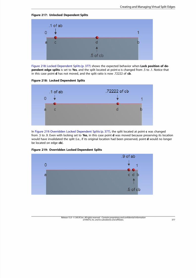
8/10/2019 ANSYS Meshing Users Guide
http://slidepdf.com/reader/full/ansys-meshing-users-guide 385/491
Figure 217: Unlocked Dependent Splits
Figure 218: Locked Dependent Splits (p. 377) shows the expected behavior when Lock position of de-pendent edge splits is set to Yes, and the split located at point c is changed from .5 to .1. Notice that
in this case point d has not moved, and the split ratio is now .72222 of cb.
Figure 218: Locked Dependent Splits
In Figure 219: Overridden Locked Dependent Splits (p. 377), the split located at point c was changedfrom .5 to .9. Even with locking set to Yes, in this case point d was moved because preserving its locationwould have invalidated the split (i.e., if its original location had been preserved, point d would no longer
be located on edge cb).
Figure 219: Overridden Locked Dependent Splits
377Release 15.0 - © SAS IP, Inc. All rights reserved. - Contains proprietary and confidential informationof ANSYS, Inc. and its subsidiaries and affiliates.
Creating and Managing Virtual Split Edges
8/10/2019 ANSYS Meshing Users Guide
http://slidepdf.com/reader/full/ansys-meshing-users-guide 386/491
Notes on Virtual Split Edges
• When the Sweep mesh method is used, the guiding edges must have consistent lengths to obtain aregular mesh in the sweep direction. You can define virtual split edges to achieve consistent lengths forthese edges.
• If your Geometry view is configured to display Shaded Exterior and Edges, you can conveniently reviewvirtual split edges by clicking the Virtual Topology group in the Tree Outline. In this mode, split edgeswill be highlighted in two different colors (automatically assigned) to draw attention to the splits.
• You cannot use the virtual split edge feature to split edges belonging to line bodies.
Creating and Managing Virtual Split Faces
When preparing geometry for meshing, it may be advantageous to split a face. This can be achievedby creating Virtual Split Face objects, which allow you to split a face along two vertices to create 1 toN virtual faces. The selected vertices must be located on the face that you want to split.
Splitting a Face
1. Insert a Virtual Topology object in the tree.
2. Choose the vertex selection filter and then in the Geometry window, pick two vertices on the face that
you want to split.
Note
• The vertices must be attached to the same face and in the same part.
• Optionally, you can create one or more Virtual Hard Vertex objects to facilitate the split
face operation. Virtual Hard Vertex objects allow you to define a hard point according to
your cursor location on a face, and then use that hard point in the split face operation.Refer to Creating and Managing Virtual Hard Vertices (p. 381).
• To see all vertices in the Geometry window, including any virtual hard vertices, make surethat the Show Vertices option is enabled.
3. Create the Virtual Split Face by doing one of the following:
• Choose Split Face at Vertices on the Virtual Topology context toolbar.
• Click right mouse button on the Virtual Topology object and select Insert> Virtual Split Face at
Vertices from the context menu.
Release 15.0 - © SAS IP, Inc. All rights reserved. - Contains proprietary and confidential informationof ANSYS, Inc. and its subsidiaries and affiliates.378
Virtual Topology
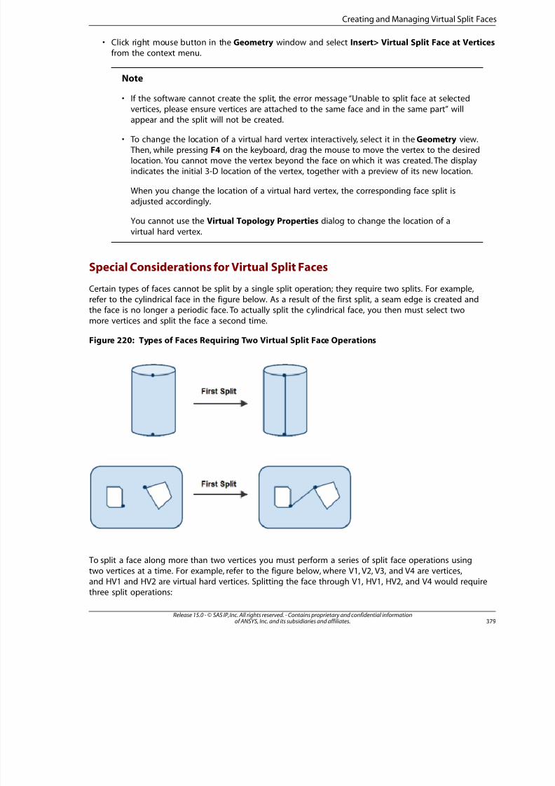
8/10/2019 ANSYS Meshing Users Guide
http://slidepdf.com/reader/full/ansys-meshing-users-guide 387/491
• Click right mouse button in the Geometry window and select Insert> Virtual Split Face at Verticesfrom the context menu.
Note
• If the software cannot create the split, the error message “Unable to split face at selectedvertices, please ensure vertices are attached to the same face and in the same part” will
appear and the split will not be created.
• To change the location of a virtual hard vertex interactively, select it in the Geometry view. Then, while pressing F4 on the keyboard, drag the mouse to move the vertex to the desiredlocation. You cannot move the vertex beyond the face on which it was created. The displayindicates the initial 3-D location of the vertex, together with a preview of its new location.
When you change the location of a virtual hard vertex, the corresponding face split isadjusted accordingly.
You cannot use the Virtual Topology Properties dialog to change the location of a
virtual hard vertex.
Special Considerations for Virtual Split Faces
Certain types of faces cannot be split by a single split operation; they require two splits. For example,refer to the cylindrical face in the figure below. As a result of the first split, a seam edge is created andthe face is no longer a periodic face. To actually split the cylindrical face, you then must select two
more vertices and split the face a second time.
Figure 220: Types of Faces Requiring Two Virtual Split Face Operations
To split a face along more than two vertices you must perform a series of split face operations using
two vertices at a time. For example, refer to the figure below, where V1, V2, V3, and V4 are vertices,and HV1 and HV2 are virtual hard vertices. Splitting the face through V1, HV1, HV2, and V4 would requirethree split operations:
379Release 15.0 - © SAS IP, Inc. All rights reserved. - Contains proprietary and confidential informationof ANSYS, Inc. and its subsidiaries and affiliates.
Creating and Managing Virtual Split Faces
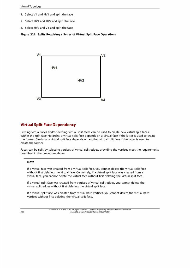
8/10/2019 ANSYS Meshing Users Guide
http://slidepdf.com/reader/full/ansys-meshing-users-guide 388/491
1. Select V1 and HV1 and split the face.
2. Select HV1 and HV2 and split the face.
3. Select HV2 and V4 and split the face.
Figure 221: Splits Requiring a Series of Virtual Split Face Operations
Virtual Split Face DependencyExisting virtual faces and/or existing virtual split faces can be used to create new virtual split faces.Within the split face hierarchy, a virtual split face depends on a virtual face if the latter is used to create
the former. Similarly, a virtual split face depends on another virtual split face if the latter is used tocreate the former.
Faces can be split by selecting vertices of virtual split edges, providing the vertices meet the requirementsdescribed in the procedure above.
Note
If a virtual face was created from a virtual split face, you cannot delete the virtual split facewithout first deleting the virtual face. Conversely, if a virtual split face was created from avirtual face, you cannot delete the virtual face without first deleting the virtual split face.
If a virtual split face was created from vertices of virtual split edges, you cannot delete thevirtual split edges without first deleting the virtual split face.
If a virtual split face was created from virtual hard vertices, you cannot delete the virtual hard
vertices without first deleting the virtual split face.
Release 15.0 - © SAS IP, Inc. All rights reserved. - Contains proprietary and confidential informationof ANSYS, Inc. and its subsidiaries and affiliates.380
Virtual Topology
8/10/2019 ANSYS Meshing Users Guide
http://slidepdf.com/reader/full/ansys-meshing-users-guide 389/491
8/10/2019 ANSYS Meshing Users Guide
http://slidepdf.com/reader/full/ansys-meshing-users-guide 390/491
operation, the fillet is re-added to the CAD model and refreshed, the virtual cell will be restored. Whena virtual entity becomes underdefined due to a geometry operation, a message is issued. You might
be able to view partial Virtual Entities by right-clicking on the Show Problematic Geometry message.
Underdefined Virtual Topologies are not displayed in Virtual Topology graphics, nor are they includedin Virtual Topology statistics.
NoteIf you suppress a part or all bodies in a multibody part in the DesignModeler application,and refresh the geometry in the Meshing application, any virtual topology that had beendefined on those bodies will be removed. The virtual topology will not be removed if onlysome bodies within a multibody part are suppressed in DesignModeler.
Using Named Selections with Virtual Topology
If you are using Named Selections with virtual topology and you subsequently modify the virtual topology,
you must manually update the Named Selections. For example, if you create a Named Selection todefine local inflation and then define virtual topology on that Named Selection, you must update theNamed Selection before generating the mesh or the inflation will not be defined correctly. This limitation
does not always occur if you perform a similar operation using the DesignModeler application. For ex-ample, after you perform a merge operation in DesignModeler, the software may be able to relink theNamed Selection to the topology automatically when the geometry is refreshed.
Cycling Through Virtual Entities in the Geometry Window
You can use the and buttons on the Virtual Topology context toolbar to cycle through virtualtopology entities in the sequence in which they were created and display them in the Geometry window.
1. In the Geometry window, select a virtual entity.
2. On the Virtual Topology context toolbar, click or .
Remember the following information when using and :
• and are grayed out until at least one virtual entity has been defined.
• If no virtual entities are selected, clicking displays the first virtual entity in the sequence and clicking
displays the last virtual entity in the sequence.
• If the currently selected virtual entity is the last in the sequence, clicking displays the first virtual entity
in the sequence. If the currently selected virtual entity is the first in the sequence, clicking displays the
last virtual entity in the sequence.
• If using when multiple virtual entities are selected, the entity that has the highest ID (based on the
order in which the entities were created) is considered to be the current selection, and clicking displaysthe entity that follows it.
• If using when multiple virtual entities are selected, the entity that has the lowest ID (based on the order
in which the entities were created) is considered to be the current selection, and clicking displays theentity that precedes it.
Release 15.0 - © SAS IP, Inc. All rights reserved. - Contains proprietary and confidential informationof ANSYS, Inc. and its subsidiaries and affiliates.382
Virtual Topology

8/10/2019 ANSYS Meshing Users Guide
http://slidepdf.com/reader/full/ansys-meshing-users-guide 391/491
8/10/2019 ANSYS Meshing Users Guide
http://slidepdf.com/reader/full/ansys-meshing-users-guide 392/491
virtual split edges, as well as virtual split faces and/or virtual hard vertices exist. Otherwise, use theDelete All Virtual Entities option.
1. Highlight the Virtual Topology object in the Tree Outline.
2. Right-click on either the Virtual Topology object in the Tree Outline, or in the Geometry window. SelectDelete All Virtual Split Edges.
3. Answer Yes at the prompt.
Deleting All Virtual Split Faces
You can use the Delete All Virtual Split Faces option to delete all virtual split faces (the virtual topologygroup itself, including any virtual cells, virtual split edges, or virtual hard vertices, will not be deleted). This option is available only when the Virtual Topology object in the Tree Outline is highlighted and
virtual split faces, as well as virtual split edges and/or virtual hard vertices exist. Otherwise, use theDelete All Virtual Entities option.
1. Highlight the Virtual Topology object in the Tree Outline.
2. Right-click on either the Virtual Topology object in the Tree Outline, or in the Geometry window. SelectDelete All Virtual Split Faces.
3. Answer Yes at the prompt.
Deleting All Virtual Hard Vertices
You can use the Delete All Virtual Hard Vertices option to delete all virtual hard vertices (the virtualtopology group itself, including any virtual cells, virtual split faces, or virtual split edges, will not be
deleted). This option is available only when the Virtual Topology object in the Tree Outline is highlightedand virtual hard vertices, as well as virtual split faces and/or virtual split edges exist. Otherwise, use theDelete All Virtual Entities option.
1. Highlight the Virtual Topology object in the Tree Outline.
2. Right-click on either the Virtual Topology object in the Tree Outline, or in the Geometry window. SelectDelete All Virtual Hard Vertices.
3. Answer Yes at the prompt.
Deleting Selected Virtual Entities
You can use the Delete Selected Virtual Entities (And Dependents) option to delete selected virtualtopology entities, along with any dependents if applicable.
To use a right mouse button click:
1. Highlight any object in the Tree Outline (for example, the Geometry or Mesh object).
2. In the Geometry window, select the virtual entities that you want to delete.
3. Right-click and select Delete Selected Virtual Entities (And Dependents).
4. Answer Yes at the prompt.
Release 15.0 - © SAS IP, Inc. All rights reserved. - Contains proprietary and confidential informationof ANSYS, Inc. and its subsidiaries and affiliates.384
Virtual Topology
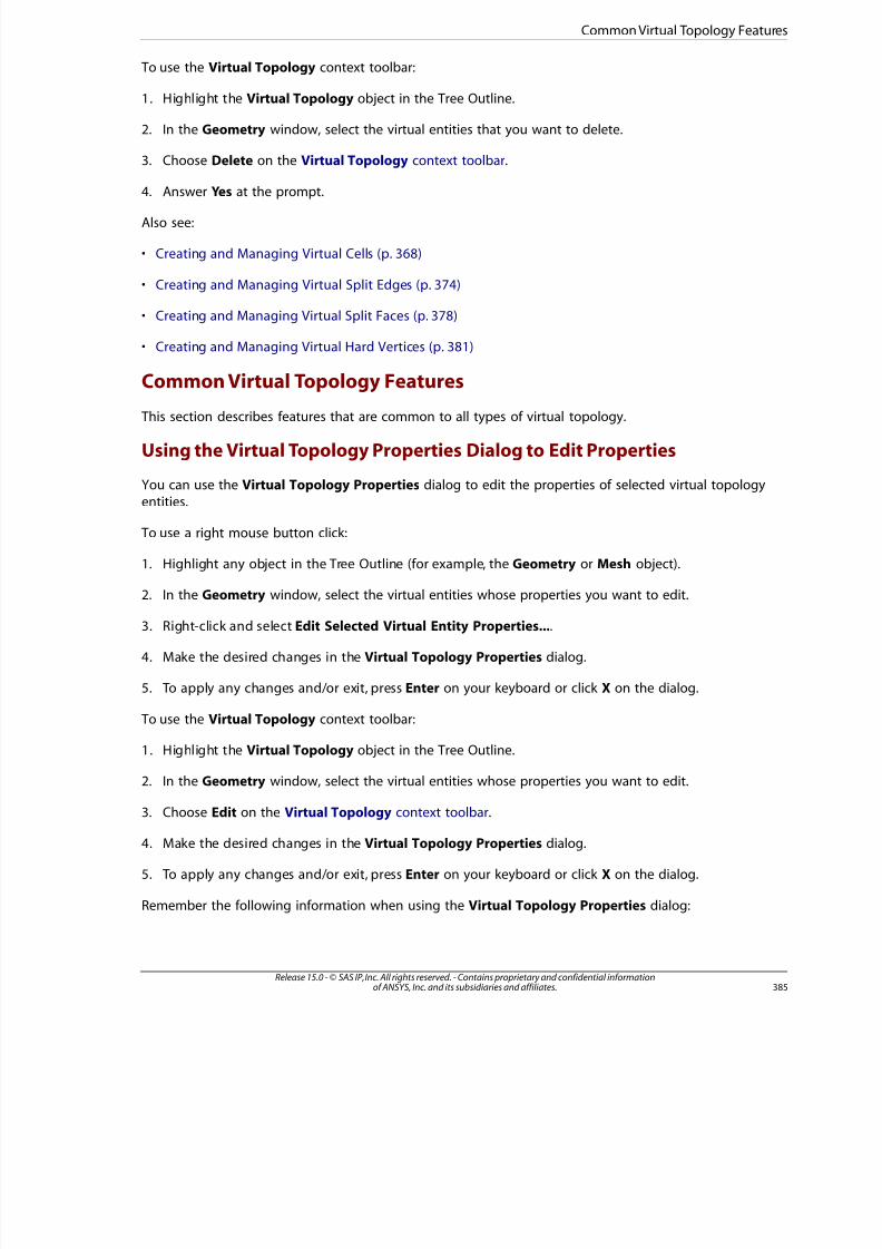
8/10/2019 ANSYS Meshing Users Guide
http://slidepdf.com/reader/full/ansys-meshing-users-guide 393/491
To use the Virtual Topology context toolbar:
1. Highlight the Virtual Topology object in the Tree Outline.
2. In the Geometry window, select the virtual entities that you want to delete.
3. Choose Delete on the Virtual Topology context toolbar.
4. Answer Yes at the prompt.
Also see:
• Creating and Managing Virtual Cells (p. 368)
• Creating and Managing Virtual Split Edges (p. 374)
• Creating and Managing Virtual Split Faces (p. 378)
• Creating and Managing Virtual Hard Vertices (p. 381)
Common Virtual Topology Features This section describes features that are common to all types of virtual topology.
Using the Virtual Topology Properties Dialog to Edit Properties
You can use the Virtual Topology Properties dialog to edit the properties of selected virtual topologyentities.
To use a right mouse button click:
1. Highlight any object in the Tree Outline (for example, the Geometry or Mesh object).
2. In the Geometry window, select the virtual entities whose properties you want to edit.
3. Right-click and select Edit Selected Virtual Entity Properties....
4. Make the desired changes in the Virtual Topology Properties dialog.
5. To apply any changes and/or exit, press Enter on your keyboard or click X on the dialog.
To use the Virtual Topology context toolbar:
1. Highlight the Virtual Topology object in the Tree Outline.
2. In the Geometry window, select the virtual entities whose properties you want to edit.
3. Choose Edit on the Virtual Topology context toolbar.
4. Make the desired changes in the Virtual Topology Properties dialog.
5. To apply any changes and/or exit, press Enter on your keyboard or click X on the dialog.
Remember the following information when using the Virtual Topology Properties dialog:
385Release 15.0 - © SAS IP, Inc. All rights reserved. - Contains proprietary and confidential informationof ANSYS, Inc. and its subsidiaries and affiliates.
Common Virtual Topology Features
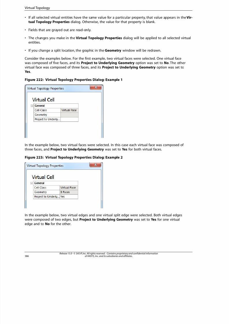
8/10/2019 ANSYS Meshing Users Guide
http://slidepdf.com/reader/full/ansys-meshing-users-guide 394/491
• If all selected virtual entities have the same value for a particular property, that value appears in the Vir-tual Topology Properties dialog. Otherwise, the value for that property is blank.
• Fields that are grayed out are read-only.
• The changes you make in the Virtual Topology Properties dialog will be applied to all selected virtualentities.
• If you change a split location, the graphic in the Geometry window will be redrawn.
Consider the examples below. For the first example, two virtual faces were selected. One virtual facewas composed of five faces, and its Project to Underlying Geometry option was set to No. The other
virtual face was composed of three faces, and its Project to Underlying Geometry option was set toYes.
Figure 222: Virtual Topology Properties Dialog: Example 1
In the example below, two virtual faces were selected. In this case each virtual face was composed of three faces, and Project to Underlying Geometry was set to Yes for both virtual faces.
Figure 223: Virtual Topology Properties Dialog: Example 2
In the example below, two virtual edges and one virtual split edge were selected. Both virtual edgeswere composed of two edges, but Project to Underlying Geometry was set to Yes for one virtualedge and to No for the other.
Release 15.0 - © SAS IP, Inc. All rights reserved. - Contains proprietary and confidential informationof ANSYS, Inc. and its subsidiaries and affiliates.386
Virtual Topology
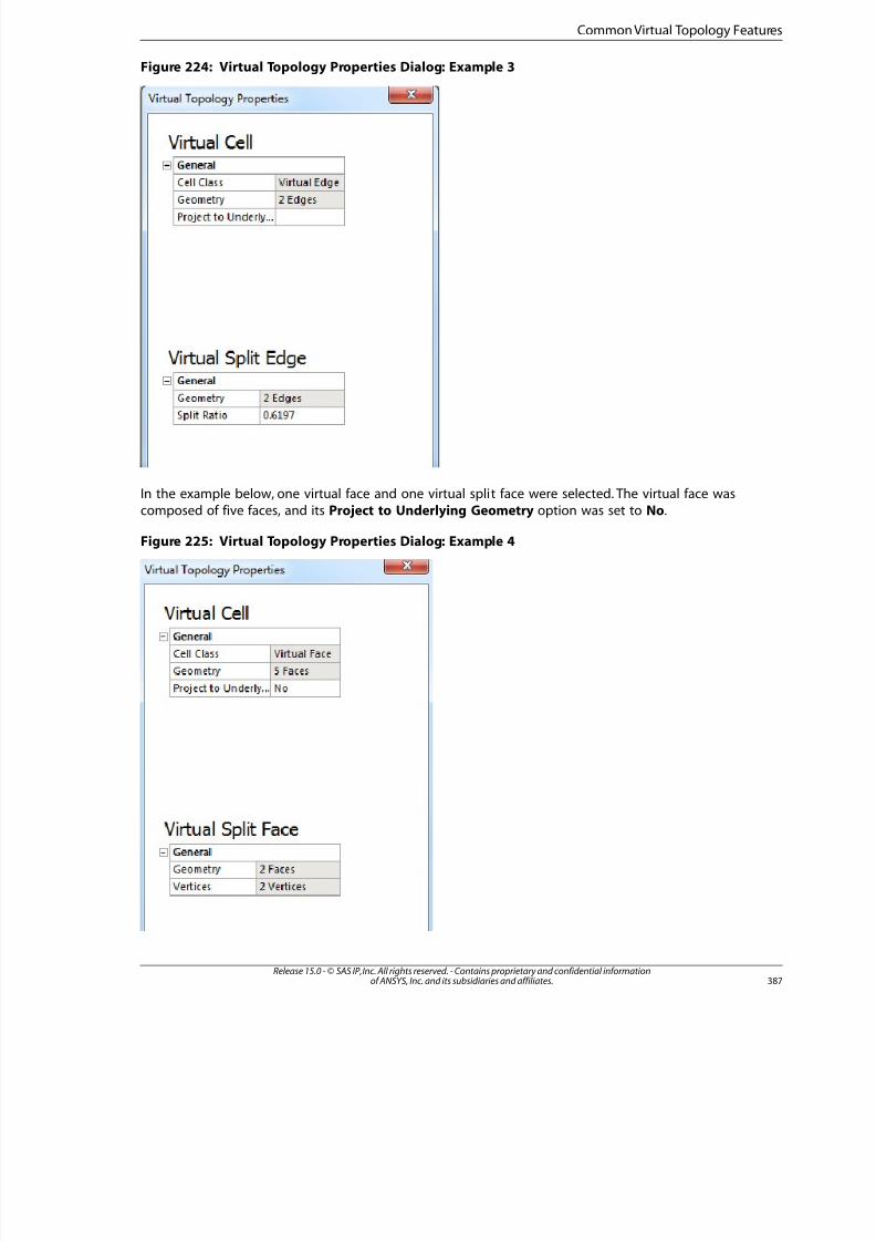
8/10/2019 ANSYS Meshing Users Guide
http://slidepdf.com/reader/full/ansys-meshing-users-guide 395/491
Figure 224: Virtual Topology Properties Dialog: Example 3
In the example below, one virtual face and one virtual split face were selected. The virtual face wascomposed of five faces, and its Project to Underlying Geometry option was set to No.
Figure 225: Virtual Topology Properties Dialog: Example 4
387Release 15.0 - © SAS IP, Inc. All rights reserved. - Contains proprietary and confidential informationof ANSYS, Inc. and its subsidiaries and affiliates.
Common Virtual Topology Features
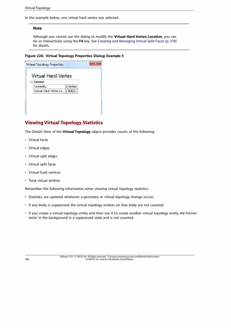
8/10/2019 ANSYS Meshing Users Guide
http://slidepdf.com/reader/full/ansys-meshing-users-guide 396/491
In the example below, one virtual hard vertex was selected.
Note
Although you cannot use the dialog to modify the Virtual Hard Vertex Location, you can
do so interactively using the F4 key. See Creating and Managing Virtual Split Faces (p. 378)for details.
Figure 226: Virtual Topology Properties Dialog: Example 5
Viewing Virtual Topology Statistics
The Details View of the Virtual Topology object provides counts of the following:
• Virtual faces
• Virtual edges
• Virtual split edges
• Virtual split faces
• Virtual hard vertices
• Total virtual entities
Remember the following information when viewing virtual topology statistics:
• Statistics are updated whenever a geometry or virtual topology change occurs.
• If any body is suppressed, the virtual topology entities on that body are not counted.
• If you create a virtual topology entity and then use it to create another virtual topology entity, the former
exists in the background in a suppressed state and is not counted.
Release 15.0 - © SAS IP, Inc. All rights reserved. - Contains proprietary and confidential informationof ANSYS, Inc. and its subsidiaries and affiliates.388
Virtual Topology

8/10/2019 ANSYS Meshing Users Guide
http://slidepdf.com/reader/full/ansys-meshing-users-guide 397/491
Meshing: Named Selections and Regions for ANSYS CFX
There are a number of places in the ANSYS Workbench and CFX applications where geometric facesand regions of mesh can be grouped together and assigned names. While this provides a large amountof flexibility, it can lead to confusion. In the 15.0 release, there is more control over which groups of
names are loaded into CFX to help simplify this issue. This document describes the ‘best practice’ forregion definitions for the 15.0 release and is targeted mainly at ANSYS CFD users of the DesignModeler,Meshing, and CFX applications.
Note
Refer to Passing Named Selections to the Solver (p. 352) for related information.
Defining Names in the DesignModeler Application or the Meshing Application
When creating or importing geometry in the DesignModeler application or editing a mesh in theMeshing application, Named Selections can be defined in terms of one or more CAD faces. If it is desirablefor these Named Selections to be available in CFX-Pre, then they must adhere to these simple rules:Named Selections should not overlap or be defined as multi-dimensional and all Named Selections
must have unique names.
Importing DesignModeler Named Selections into the Meshing Application
If the Named Selections defined in the DesignModeler application are required in the Meshing application
you must set the appropriate geometry import options to ensure the Named Selections will be transferredproperly:
1. From the ANSYS Workbench Menu Bar, select Tools> Options.
2. In the left pane of the Options dialog box, select Geometry Import.
3. In the right pane of the Options dialog box, select the Named Selections check box and either
clear the Filtering Prefixes field (to import all names) or set it to the appropriate filter if required.
The next time that you attach geometry containing Named Selections and launch the Meshing applic-ation, the application will start, load the geometry, and load any Named Selections previously definedfor that geometry. The preferences you set on the Options dialog box are local settings and affect only
you.
If a mesh is generated, the Named Selections defined in the DesignModeler application will be availablewhen the mesh is imported into CFX-Pre.
Note
For detailed descriptions of the geometry import options, see the CAD Integration sectionin the ANSYS Workbench help.
389Release 15.0 - © SAS IP, Inc. All rights reserved. - Contains proprietary and confidential informationof ANSYS, Inc. and its subsidiaries and affiliates.

8/10/2019 ANSYS Meshing Users Guide
http://slidepdf.com/reader/full/ansys-meshing-users-guide 398/491
Using Multiple Mesh Methods
Named Selections can be defined in the Meshing application, the DesignModeler application, or supportedCAD systems. When the resulting mesh is loaded into CFX-Pre, all of these Named Selections are available.Control over which names are imported with the mesh is available in the Mesh Import options.
It is possible to define Named Selections that conflict with some virtual topology, or do not conformto the CFX Topology Model in some other way. Such Named Selections will not be imported into CFX-Pre.
If a Named Selection is created that contains characters not supported in CFX-Pre names, these nameswill be modified on import to remove the illegal characters.
Invalid Named Selections
The use of Virtual Topology within the Meshing application can invalidate Named Selection definitions.Consider the case where a Named Selection ‘Region1’ is defined in terms of 4 CAD faces (1, 2, 3 and 4).
If this geometry is then loaded into the Meshing application and Virtual Topology is used to merge 2of these faces (3 and 4), the original Named Selection can no longer be resolved. In CFX-Pre, the Named
Selection will be modified so that it only refers to the ‘resolvable’ faces. Hence, in CFX-Pre, the NamedSelection ‘Region1’ would be defined in terms of faces 1 and 2 only.
Named Selections Involving Interior Faces
If an interior face (for example, a face that is shared between two bodies in the same part in Design-
Modeler) is included in a Named Selection in the Meshing application, then the corresponding locationin CFX-Pre will be a Composite region that includes two Primitive regions: one for each side of the in-terior face. Care should be taken when using the resulting Composite region for evaluating expressions
and performing calculations: for example, areas evaluated on such a Composite region would be likelyto give double the expected result (since the area is evaluated over both of the primitive regions thatform the two sides of the interior face) and mass flows will be approximately zero (since the mass flow
is evaluated on both of the primitive regions and will have the opposite sign on each). You can optionallyedit the Composite region in CFX-Pre to include only one of the primitive regions.
Release 15.0 - © SAS IP, Inc. All rights reserved. - Contains proprietary and confidential informationof ANSYS, Inc. and its subsidiaries and affiliates.390
Named Selections and Regions for ANSYS CFX
8/10/2019 ANSYS Meshing Users Guide
http://slidepdf.com/reader/full/ansys-meshing-users-guide 399/491
Meshing: Troubleshooting
This section is intended to provide you with tips and strategies for avoiding and handling problemsthat may occur when using the Meshing application. Topics include:
• Using a Localized Operating System on Linux (p. 391)
• Recommended First Course of Action for Meshing Failures (p. 392)
• Understanding Messaging (p. 393)
• Understanding States (p. 394)
• Shape Checks and Meshing Failures (p. 394)
• Handling Selective Meshing Failures (p. 395)
• Handling Patch Independent Meshing Failures (p. 395)
• Handling Patch Conforming Tetrahedral, Quad Dominant, and All Triangle Meshing Failures (p. 396)
• Handling General Sweep Meshing Failures (p. 397)
• Handling Thin Sweep Meshing Failures (p. 397)
• Handling General MultiZone Meshing Failures (p. 398)
• Handling Failed Mesh Connections (p. 400)
• Avoiding Bad Feature Capturing in Assembly Meshing (p. 400)
• Handling Assembly Meshing Failures Due to Min Size (p. 400)
• Handling Assembly Meshing Failures Due to Flow Volume Leaks (p. 401)
• Handling Assembly Meshing Inflation Problems (p. 403)
• Tips for Using Virtual Topology (p. 403)
• Meshing Complicated Models (p. 403)
• Handling Fracture Meshing Problems (p. 405)
Using a Localized Operating System on Linux
If you are using a localized operating system (such as French or German) on Linux, you must performadditional steps in order for the Meshing application to recognize the correct numerical format. Referto the platform details section of the ANSYS, Inc. Linux Installation Guide for details.
39Release 15.0 - © SAS IP, Inc. All rights reserved. - Contains proprietary and confidential informationof ANSYS, Inc. and its subsidiaries and affiliates.
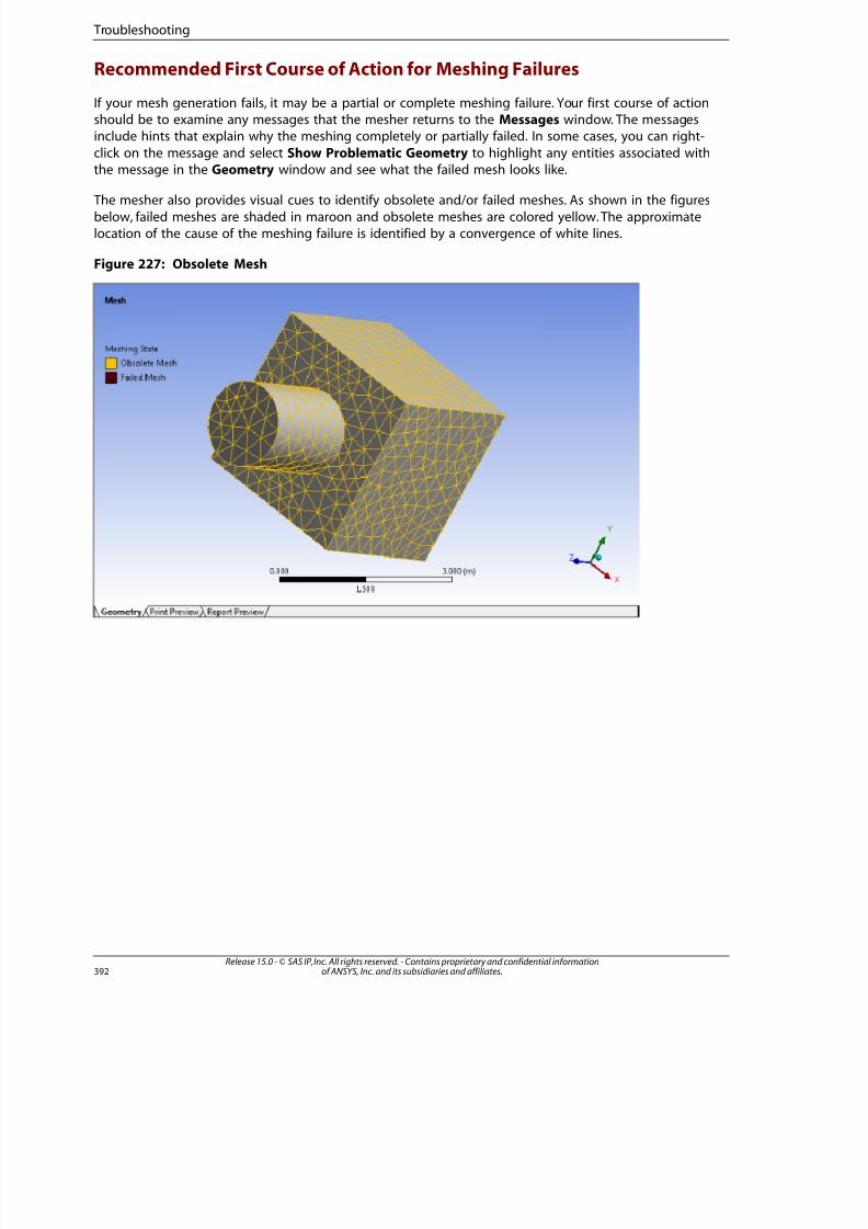
8/10/2019 ANSYS Meshing Users Guide
http://slidepdf.com/reader/full/ansys-meshing-users-guide 400/491
Recommended First Course of Action for Meshing Failures
If your mesh generation fails, it may be a partial or complete meshing failure. Your first course of actionshould be to examine any messages that the mesher returns to the Messages window. The messagesinclude hints that explain why the meshing completely or partially failed. In some cases, you can right-
click on the message and select Show Problematic Geometry to highlight any entities associated withthe message in the Geometry window and see what the failed mesh looks like.
The mesher also provides visual cues to identify obsolete and/or failed meshes. As shown in the figures
below, failed meshes are shaded in maroon and obsolete meshes are colored yellow. The approximatelocation of the cause of the meshing failure is identified by a convergence of white lines.
Figure 227: Obsolete Mesh
Release 15.0 - © SAS IP, Inc. All rights reserved. - Contains proprietary and confidential informationof ANSYS, Inc. and its subsidiaries and affiliates.392
Troubleshooting
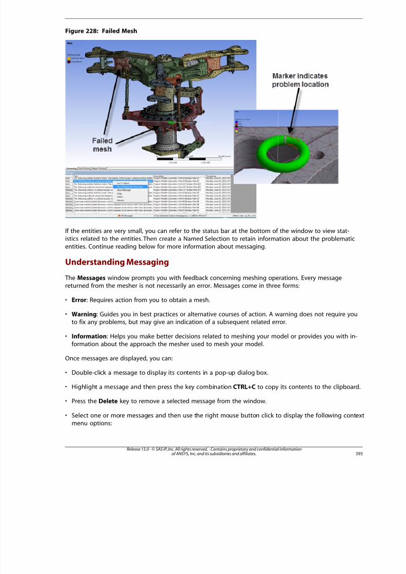
8/10/2019 ANSYS Meshing Users Guide
http://slidepdf.com/reader/full/ansys-meshing-users-guide 401/491
Figure 228: Failed Mesh
If the entities are very small, you can refer to the status bar at the bottom of the window to view stat-
istics related to the entities. Then create a Named Selection to retain information about the problematicentities. Continue reading below for more information about messaging.
Understanding Messaging
The Messages window prompts you with feedback concerning meshing operations. Every messagereturned from the mesher is not necessarily an error. Messages come in three forms:
• Error: Requires action from you to obtain a mesh.
• Warning: Guides you in best practices or alternative courses of action. A warning does not require youto fix any problems, but may give an indication of a subsequent related error.
• Information: Helps you make better decisions related to meshing your model or provides you with in-formation about the approach the mesher used to mesh your model.
Once messages are displayed, you can:
• Double-click a message to display its contents in a pop-up dialog box.
• Highlight a message and then press the key combination CTRL+C to copy its contents to the clipboard.
• Press the Delete key to remove a selected message from the window.
• Select one or more messages and then use the right mouse button click to display the following contexmenu options:
393Release 15.0 - © SAS IP, Inc. All rights reserved. - Contains proprietary and confidential informationof ANSYS, Inc. and its subsidiaries and affiliates.
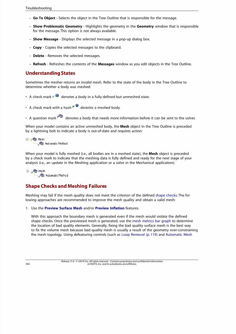
8/10/2019 ANSYS Meshing Users Guide
http://slidepdf.com/reader/full/ansys-meshing-users-guide 402/491
– Go To Object - Selects the object in the Tree Outline that is responsible for the message.
– Show Problematic Geometry - Highlights the geometry in the Geometry window that is responsiblefor the message. This option is not always available.
– Show Message - Displays the selected message in a pop-up dialog box.
– Copy - Copies the selected messages to the clipboard.
– Delete - Removes the selected messages.
– Refresh - Refreshes the contents of the Messages window as you edit objects in the Tree Outline.
Understanding States
Sometimes the mesher returns an invalid mesh. Refer to the state of the body in the Tree Outline todetermine whether a body was meshed:
• A check mark denotes a body in a fully defined but unmeshed state.
• A check mark with a hash denotes a meshed body.
• A question mark denotes a body that needs more information before it can be sent to the solver.
When your model contains an active unmeshed body, the Mesh object in the Tree Outline is precededby a lightning bolt to indicate a body is out-of-date and requires action:
When your model is fully meshed (i.e., all bodies are in a meshed state), the Mesh object is preceded
by a check mark to indicate that the meshing data is fully defined and ready for the next stage of youranalysis (i.e., an update in the Meshing application or a solve in the Mechanical application):
Shape Checks and Meshing Failures
Meshing may fail if the mesh quality does not meet the criterion of the defined shape checks. The fol-
lowing approaches are recommended to improve the mesh quality and obtain a valid mesh:
1. Use the Preview Surface Mesh and/or Preview Inflation features.
With this approach the boundary mesh is generated even if the mesh would violate the definedshape checks. Once the previewed mesh is generated, use the mesh metrics bar graph to determine
the location of bad quality elements. Generally, fixing the bad quality surface mesh is the best wayto fix the volume mesh because bad quality mesh is usually a result of the geometry over-constrainingthe mesh topology. Using defeaturing controls (such as Loop Removal (p. 119) and Automatic Mesh
Release 15.0 - © SAS IP, Inc. All rights reserved. - Contains proprietary and confidential informationof ANSYS, Inc. and its subsidiaries and affiliates.394
Troubleshooting

8/10/2019 ANSYS Meshing Users Guide
http://slidepdf.com/reader/full/ansys-meshing-users-guide 403/491
Based Defeaturing (p. 120)), pinch controls, and virtual topologies are all good strategies to removegeometry features that may cause problems for the meshing algorithms.
Note
Not all mesh methods support the use of Preview Surface Mesh and Preview Inflation.
2. Use a different shape check setting.
Some shape checks have a stricter set of criterion than others. By using a different shape check
setting a mesh might be generated, and the mesh metrics bar graph can be used to find the meshviolating the stricter shape checks. In this way, locating the problem is the first step to fixing it.
Note
You can turn off most shape checks altogether by setting Shape Checking (p. 104) to
None.
For additional information about the shape checking acceptance criterion used by ANSYS Workbench,refer to ANSYS Workbench and Mechanical APDL Application Meshing Differences (p. 59).
Handling Selective Meshing Failures
Selective meshing may lead to unexpected results in cases where a mesh control change affects onlyone body. This may in turn lead to sweep mesh failure because the source and target meshes no longer
align or the resultant change makes a body unsweepable. If desired, you can set the Allow SelectiveMeshing option to No to disable selective meshing and allow the mesh control changes to ripplethrough the entire part.
Selective meshing is not persistent for a geometry update or re-mesh operation. However, you can usethe Mesh worksheet to create a selective meshing history so that your meshing steps can be repeatedin the desired sequence. Otherwise, you may need to go through your body meshing steps manuallyif the single mesh update does not satisfy your meshing requirements. Refer to Using the Mesh Worksheet
to Create a Selective Meshing History (p. 311) for details.
Handling Patch Independent Meshing Failures
If there are gaps in your geometry and Patch Independent meshing fails, the mesh size may be setsmaller than the size of the gaps in the geometry. In such cases, try adjusting the size of the mesh inthose regions so they are larger than the geometry gap size.
395Release 15.0 - © SAS IP, Inc. All rights reserved. - Contains proprietary and confidential informationof ANSYS, Inc. and its subsidiaries and affiliates.
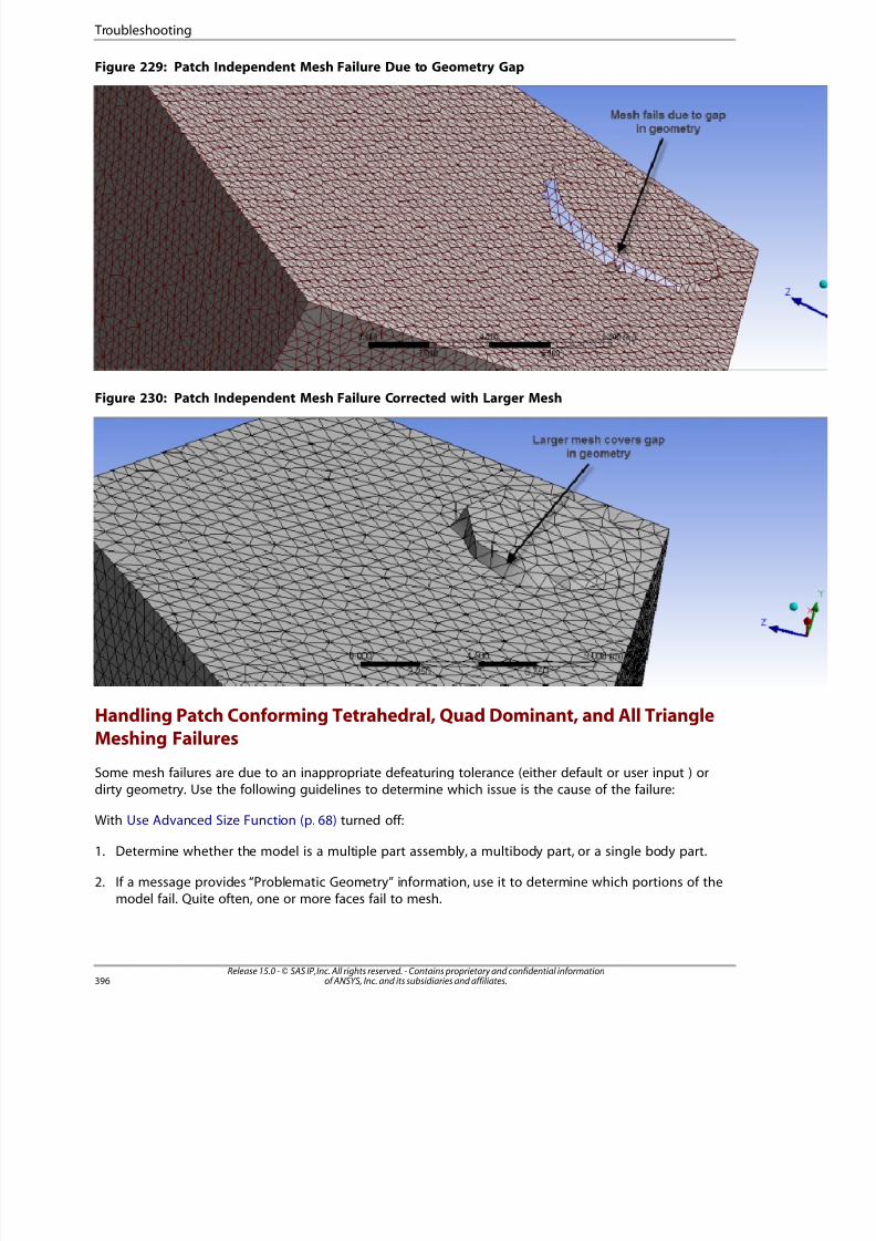
8/10/2019 ANSYS Meshing Users Guide
http://slidepdf.com/reader/full/ansys-meshing-users-guide 404/491
Figure 229: Patch Independent Mesh Failure Due to Geometry Gap
Figure 230: Patch Independent Mesh Failure Corrected with Larger Mesh
Handling Patch Conforming Tetrahedral, Quad Dominant, and All Triangle
Meshing Failures
Some mesh failures are due to an inappropriate defeaturing tolerance (either default or user input ) ordirty geometry. Use the following guidelines to determine which issue is the cause of the failure:
With Use Advanced Size Function (p. 68) turned off:
1. Determine whether the model is a multiple part assembly, a multibody part, or a single body part.
2. If a message provides “Problematic Geometry” information, use it to determine which portions of themodel fail. Quite often, one or more faces fail to mesh.
Release 15.0 - © SAS IP, Inc. All rights reserved. - Contains proprietary and confidential informationof ANSYS, Inc. and its subsidiaries and affiliates.396
Troubleshooting

8/10/2019 ANSYS Meshing Users Guide
http://slidepdf.com/reader/full/ansys-meshing-users-guide 405/491
3. If a face fails to mesh, check whether the face is “regular”; that is, make sure that it is not too skinny orhas skinny sections with misaligned edge spacings which would make it difficult to get a good mesh.
Use of virtual topologies, pinch controls, etc. may help in these situations.
4. If a face fails to mesh, check to see if the edges attached to that face may be problematic. For example
• Turn on the Show Vertices option to see if any edge is significantly faceted (i.e., has many edge split
in comparison to mesh size). The mesher will try to place a node on each vertex, so unnecessary vert
can lead to complications in meshing that may be avoidable. Use of virtual topologies, pinch controletc. may help in these situations.
• Turn on the Edge Coloring > By Connection option to see if the edge connectivity is unusual. Insome cases, the geometry connectivity may not be as expected, and this may create problems duringmeshing. These problems could be fixed in the DesignModeler application, the CAD package, or possthrough the use of virtual topologies or pinch controls.
Handling General Sweep Meshing Failures
In the event of a sweep mesh failure, the following approaches are recommended:
1. Check for contradicting edge sizings.
2. For Src/Trg Selection, use a manual setting instead of automatic.
3. Check side faces to see if they are mappable. Use of virtual topologies can help make bodies sweepabl
• Turn on the Show Vertices option to see if any edges have unnecessary splits. Extra edge splits canmake faces that appear to be mappable more difficult to map. Virtual edges can help in these cases.
• Use of virtual face splits can help make faces more mappable, as can use of the mapped face mesh
control and its advanced options.
4. Turn on the Edge Coloring > By Connection option to see if the edge connectivity is unusual. In somecases, the geometry connectivity may not be as expected, and this may create problems during meshin
These problems could be fixed in the DesignModeler application, the CAD package, or possibly throughthe use of virtual topologies.
For detailed information about the requirements and characteristics of sweep meshing, refer to MeshSweeping (p. 231).
For additional information, refer to Figure 7.36: Strategies for Avoiding Stretched Elements in theMechanical APDL help.
Handling Thin Sweep Meshing Failures
In the event of a thin sweep mesh failure, first refer to Thin Model Sweeping (p. 238) for detailed inform-ation about the requirements and characteristics of thin sweep meshing.
The Preview Source and Target Mesh and Preview Surface Mesh features do not support the thinmodel sweeper. Thus, if a failure occurs, you must use the feedback in the Messages window to determ-ine the problem:
• If Src/Trg Selection is set to Automatic Thin, determine whether the correct source/target faces are beiused. You can review the source/target faces by right-clicking the appropriate message. If incorrect
397Release 15.0 - © SAS IP, Inc. All rights reserved. - Contains proprietary and confidential informationof ANSYS, Inc. and its subsidiaries and affiliates.

8/10/2019 ANSYS Meshing Users Guide
http://slidepdf.com/reader/full/ansys-meshing-users-guide 406/491
source/target faces are being used, select the Manual Thin option on the sweep method and pick thecorrect faces manually.
• In many cases, the messages tell you to use virtual topology to merge an edge/face. Thin sweeping requiresone division through the thickness. Side edges must connect directly from source to target to complywith this rule.
• If a message tells you the target faces are not meshed, try swapping the source/target faces.
• In cases where a thin sweep body and a general sweep body are neighbors, the general sweep body hashigher priority and is meshed first. The general sweep operation may place nodes on the side area/edge
of the thin sweep body. If you receive a message describing this situation, you must apply additionalmesh controls to prevent it.
• If both source and target areas are meshed, thin sweep will fail. In this case, you must find some way toeliminate the situation.
• Thin sweep may issue warning messages telling you that the source you picked was swapped with thetarget, and that some controls on the target faces were ignored as a result. These types of warning messagesare for your reference only.
Handling General MultiZone Meshing Failures
In the event of a MultiZone mesh failure, the following approaches are recommended:
1. If using automatic source face selection, try using manual source face selection (or vice versa). Formanual source face selection, ensure that all sources and targets are selected. Refer to Using Mul-tiZone (p. 255) for more information.
2. Ensure that all side faces are mappable. Refer to MultiZone Face Mappability Guidelines (p. 262) for moreinformation. Use of virtual topologies can help make bodies sweepable:
• Turn on the Show Vertices option to see if any edges have unnecessary splits. Extra edge splits canmake faces that appear to be mappable more difficult to map. Virtual edges can help in these cases.
• Use of virtual face splits can help make faces more mappable, as can use of the mapped face meshcontrol.
3. If MultiZone doesn’t respect edge biasing, as shown in Figure 231: Edge Biasing Not Respected by Mul-
tiZone (p. 399) below, it may be because the opposite edge is split. To work around this, perform theedge biasing on the opposite edges to get a better edge distribution, as shown in Figure 232: Edge BiasingRespected by MultiZone (p. 399).
Release 15.0 - © SAS IP, Inc. All rights reserved. - Contains proprietary and confidential informationof ANSYS, Inc. and its subsidiaries and affiliates.398
Troubleshooting
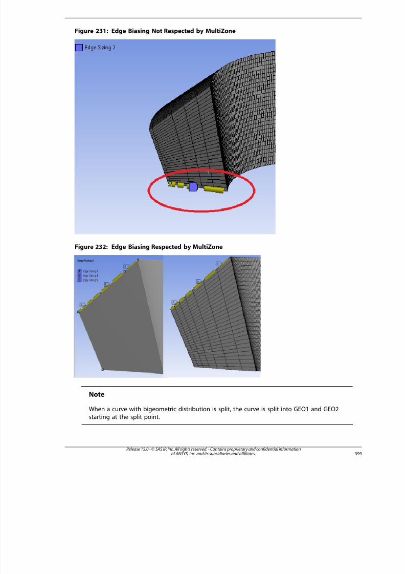
8/10/2019 ANSYS Meshing Users Guide
http://slidepdf.com/reader/full/ansys-meshing-users-guide 407/491
Figure 231: Edge Biasing Not Respected by MultiZone
Figure 232: Edge Biasing Respected by MultiZone
Note
When a curve with bigeometric distribution is split, the curve is split into GEO1 and GEO2
starting at the split point.
399Release 15.0 - © SAS IP, Inc. All rights reserved. - Contains proprietary and confidential informationof ANSYS, Inc. and its subsidiaries and affiliates.

8/10/2019 ANSYS Meshing Users Guide
http://slidepdf.com/reader/full/ansys-meshing-users-guide 408/491
4. Turn on the Edge Coloring > By Connection option to see if the edge connectivity is unusual. In somecases, the geometry connectivity may not be as expected, and this may create problems during meshing.
These problems could be fixed in the DesignModeler application, the CAD package, or possibly throughthe use of virtual topologies.
For detailed information about the requirements and characteristics of MultiZone, refer to MultiZone
Meshing (p. 251).
Handling Failed Mesh Connections
In the event of a mesh connection failure, refer to Diagnosing Failed Mesh Connections in the Mechan-ical help.
Avoiding Bad Feature Capturing in Assembly Meshing
In some cases, you may encounter bad feature capturing when using assembly meshing in the Meshingapplication, even though the faceting of the same model looks fine in ANSYS Fluent . The bad faceting
may be apparent in ANSYS Fluent only if you turn off the viewing of edges and view surfaces only. Thefollowing approaches are recommended to avoid bad feature capture:
• If you are experiencing bad feature capture, increasing facet quality can help. If you are using theDesignModeler application, increasing the value of the Facet Quality option (Tools > Options >
DesignModeler > Graphics > Facet Quality) from 5 (the default) to 10 can lead to significant improve-ments. This Facet Quality option affects models entering the Meshing application via DesignModeleronly; CAD packages have their own separate faceting controls. In particular, you should increase facet
quality in DesignModeler or your CAD package if your model contains high order NURBS surfaces and/oryour applications require the highest fidelity to your input CAD (i.e., aerospace applications, external aeroapplications, etc.). However, be aware that higher settings create large numbers of facets, which may slowdown processing or possibly lead to failures in facet generation due to insufficient memory. Refer to Facet
Quality for details about this setting in DesignModeler.
• In cases of tolerant models, the Tessellation Refinement (p. 98) control tries to avoid re-projections to theunderlying curves and surfaces at locations where the CAD tolerance exceeds the desired refinement
tolerance. In cases of significant tolerances, you may want to relax the Tessellation Refinement toleranceor even set it to None to avoid re-projections that may contribute to problems with faceting. In cases of accurate models, the default settings typically work well.
• The Sharp Angle Tool (p. 221) can be used to control the capture of features with sharp angles, as well as
to improve feature capture in general.
Handling Assembly Meshing Failures Due to Min Size
Failure in the assembly meshing algorithms is almost always related to faceting issues in relation to
minimum size. Make sure that the values of the Min Size (p. 74) and Proximity Min Size (p. 75) optionstruly represent the smallest sizes that you want the curvature and proximity size functions to capture.
By default, many meshing features operate based on the smaller of these two minimum size values.Consider the following:
1. It is strongly recommended that you ALWAYS adjust the value of Min Size /Proximity Min Size as appro-priate for your problem. Make sure that the minimum size is 1/2 of any small feature or gap that you
need to capture. Similarly, the minimum size should be about 1/10 of the diameter of the smallest pipe.For very simple cases, make sure to increase the minimum size appropriately. Failure to do so may resultin an over-refined mesh with a huge number of facets.
Release 15.0 - © SAS IP, Inc. All rights reserved. - Contains proprietary and confidential informationof ANSYS, Inc. and its subsidiaries and affiliates.400
Troubleshooting

8/10/2019 ANSYS Meshing Users Guide
http://slidepdf.com/reader/full/ansys-meshing-users-guide 409/491
2. Use local (scoped) size controls to ensure two layers of elements in any gap/thickness. If the scoped sizis smaller than the minimum size, you must adjust the Tessellation Refinement accordingly. If you add
a hard size that is smaller than the minimum size, make sure that the tolerance specified by the Tessel-lation Refinement control is now 10 times smaller than the specified hard size.
3. If you receive a warning about missing tessellations, it may help to lower the tessellation tolerance by
50%.
4. In some cases, small defects in the faceting may lead to bad quality meshes. In many of these cases, aminor modification of the minimum size or tessellation tolerance can rectify the problem.
Handling Assembly Meshing Failures Due to Flow Volume Leaks
Virtual bodies are used with assembly meshing to represent flow volumes in a model so that you can
mesh flow regions without having to model geometry to represent them. These flow volumes are ex-tracted during meshing; however, an extraction failure may occur if there are gaps between bodiesand/or faces such that the extracted flow volume would not be watertight and therefore would leak.If a leak is present, the flow volume mesh will contain only elements from the leak path (that is, surface
and line elements will be returned but volume elements will not). As a result, assembly mesh generationwill be unsuccessful and an error message will be issued. In such cases, the assembly meshing algorithmsdetect and trace the leaks and display their leak paths graphically as follows:
• Any time there is an exterior leak (that is, the mesh leaks to the outside of the model), it will be detecteby the Meshing application. However, the leak path will be displayed only if you have defined a virtualbody and specified a material point in the flow volume void. For exterior leaks, tracing occurs from thebounding box to all defined material points.
When a material point is inside a virtual body, you must also set Used By Fluid Surface to Yes whendefining the virtual body, and then define the appropriate set of fluid surfaces by selecting the facesof the virtual body and assigning them to the group.
• Interior leaks involve leak tracing between material points; thus for an interior leak to be identified, youmust define two or more virtual bodies and specify a material point in each flow volume void.
If a leak is detected, the leak path should clearly indicate its location, in which case you should returnthe model to the DesignModeler application or your CAD system to close the gap that is causing the
leak (for example, by adding a face or moving a body).
Note
• If you suppress a virtual body, any leak path associated with it will be hidden from view in theGeometry window.
• In some assembly meshing cases, contact sizing can also be used for closing leaks discoveredduring meshing. Refer to Applying Contact Sizing (p. 301) for details.
The figure below shows the leak path for a failed assembly mesh.
40Release 15.0 - © SAS IP, Inc. All rights reserved. - Contains proprietary and confidential informationof ANSYS, Inc. and its subsidiaries and affiliates.
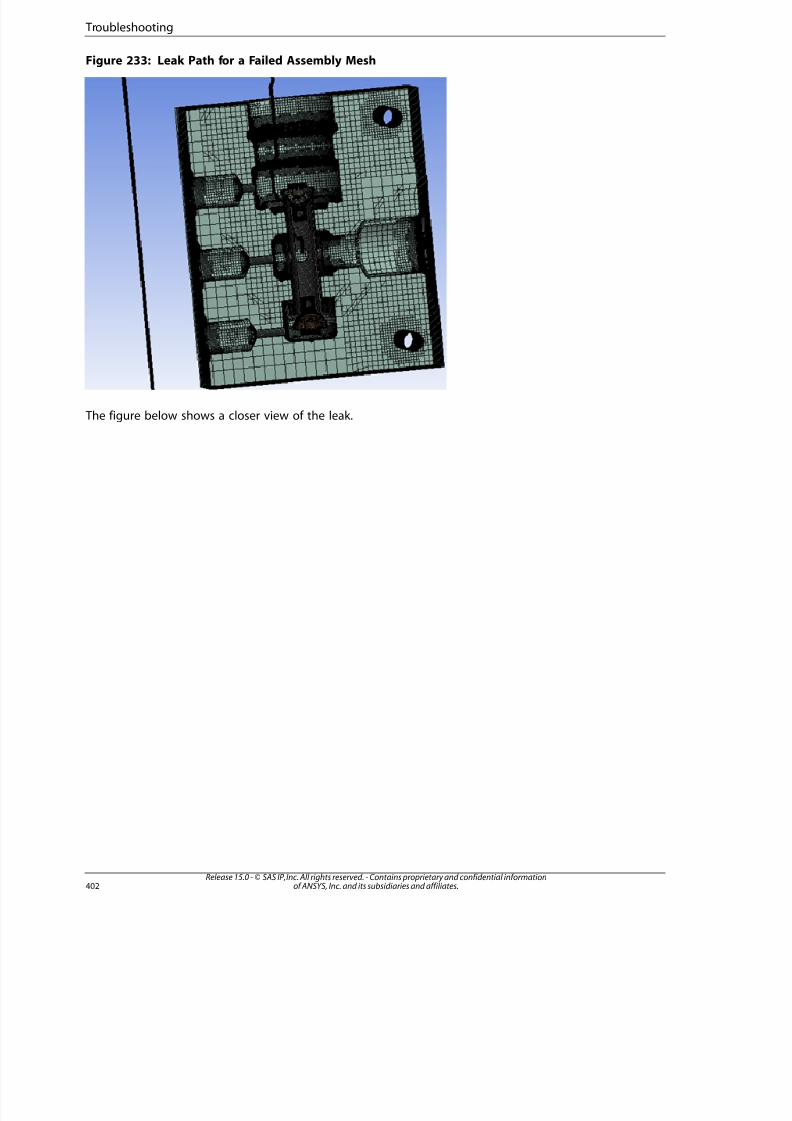
8/10/2019 ANSYS Meshing Users Guide
http://slidepdf.com/reader/full/ansys-meshing-users-guide 410/491
Figure 233: Leak Path for a Failed Assembly Mesh
The figure below shows a closer view of the leak.
Release 15.0 - © SAS IP, Inc. All rights reserved. - Contains proprietary and confidential informationof ANSYS, Inc. and its subsidiaries and affiliates.402
Troubleshooting
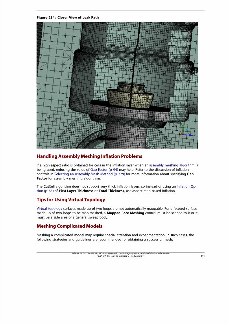
8/10/2019 ANSYS Meshing Users Guide
http://slidepdf.com/reader/full/ansys-meshing-users-guide 411/491
Figure 234: Closer View of Leak Path
Handling Assembly Meshing Inflation Problems
If a high aspect ratio is obtained for cells in the inflation layer when an assembly meshing algorithm is
being used, reducing the value of Gap Factor (p. 94) may help. Refer to the discussion of inflationcontrols in Selecting an Assembly Mesh Method (p. 279) for more information about specifying GapFactor for assembly meshing algorithms.
The CutCell algorithm does not support very thick inflation layers, so instead of using an Inflation Op-tion (p. 83) of First Layer Thickness or Total Thickness, use aspect ratio-based inflation.
Tips for Using Virtual Topology
Virtual topology surfaces made up of two loops are not automatically mappable. For a faceted surfacemade up of two loops to be map meshed, a Mapped Face Meshing control must be scoped to it or itmust be a side area of a general sweep body.
Meshing Complicated Models
Meshing a complicated model may require special attention and experimentation. In such cases, the
following strategies and guidelines are recommended for obtaining a successful mesh:
403Release 15.0 - © SAS IP, Inc. All rights reserved. - Contains proprietary and confidential informationof ANSYS, Inc. and its subsidiaries and affiliates.
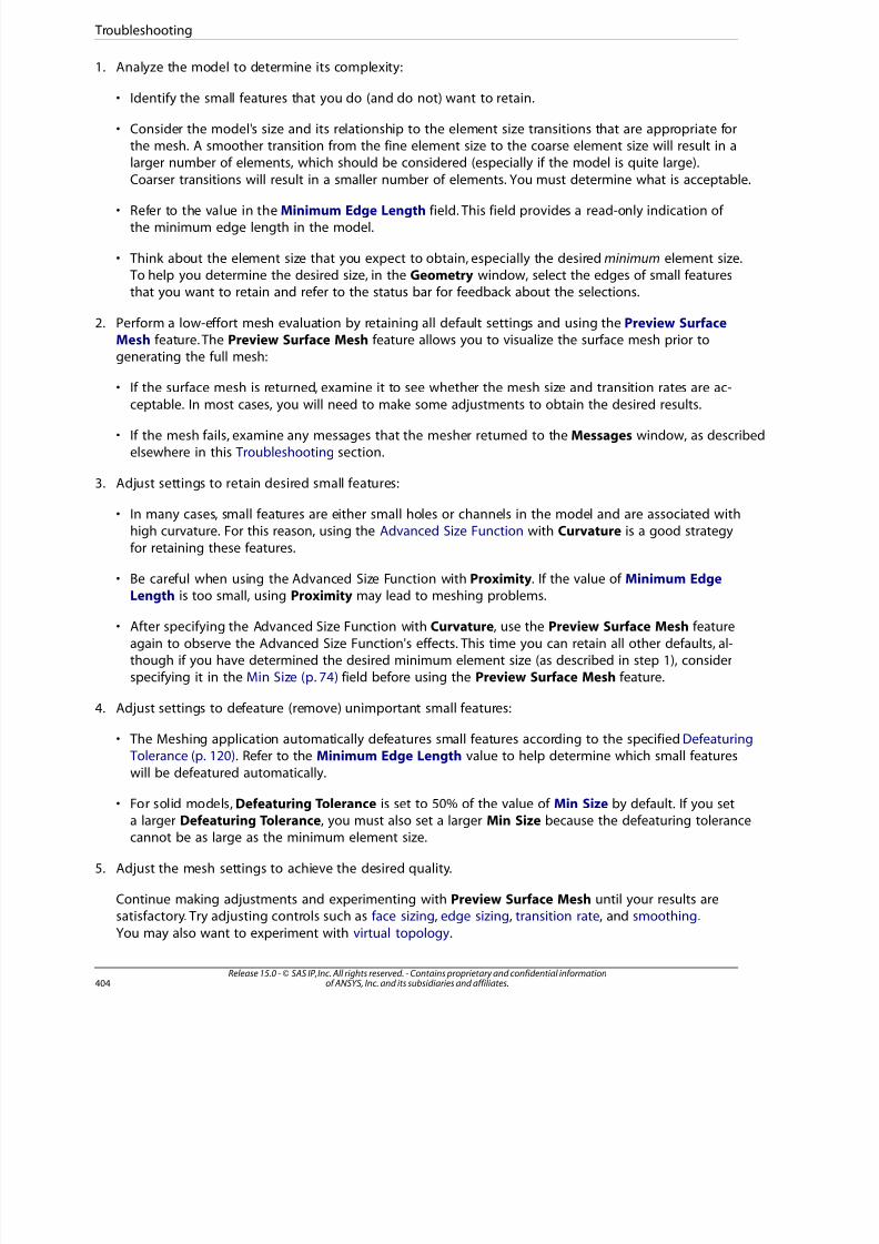
8/10/2019 ANSYS Meshing Users Guide
http://slidepdf.com/reader/full/ansys-meshing-users-guide 412/491
1. Analyze the model to determine its complexity:
• Identify the small features that you do (and do not) want to retain.
• Consider the model's size and its relationship to the element size transitions that are appropriate forthe mesh. A smoother transition from the fine element size to the coarse element size will result in alarger number of elements, which should be considered (especially if the model is quite large).
Coarser transitions will result in a smaller number of elements. You must determine what is acceptable.
• Refer to the value in the Minimum Edge Length field. This field provides a read-only indication of the minimum edge length in the model.
• Think about the element size that you expect to obtain, especially the desired minimum element size. To help you determine the desired size, in the Geometry window, select the edges of small featuresthat you want to retain and refer to the status bar for feedback about the selections.
2. Perform a low-effort mesh evaluation by retaining all default settings and using the Preview SurfaceMesh feature. The Preview Surface Mesh feature allows you to visualize the surface mesh prior togenerating the full mesh:
• If the surface mesh is returned, examine it to see whether the mesh size and transition rates are ac-ceptable. In most cases, you will need to make some adjustments to obtain the desired results.
• If the mesh fails, examine any messages that the mesher returned to the Messages window, as describedelsewhere in this Troubleshooting section.
3. Adjust settings to retain desired small features:
• In many cases, small features are either small holes or channels in the model and are associated withhigh curvature. For this reason, using the Advanced Size Function with Curvature is a good strategy
for retaining these features.
• Be careful when using the Advanced Size Function with Proximity. If the value of Minimum EdgeLength is too small, using Proximity may lead to meshing problems.
• After specifying the Advanced Size Function with Curvature, use the Preview Surface Mesh feature
again to observe the Advanced Size Function's effects. This time you can retain all other defaults, al-though if you have determined the desired minimum element size (as described in step 1), considerspecifying it in the Min Size (p. 74) field before using the Preview Surface Mesh feature.
4. Adjust settings to defeature (remove) unimportant small features:
• The Meshing application automatically defeatures small features according to the specified Defeaturing Tolerance (p. 120). Refer to the Minimum Edge Length value to help determine which small features
will be defeatured automatically.
• For solid models, Defeaturing Tolerance is set to 50% of the value of Min Size by default. If you seta larger Defeaturing Tolerance, you must also set a larger Min Size because the defeaturing tolerancecannot be as large as the minimum element size.
5. Adjust the mesh settings to achieve the desired quality.
Continue making adjustments and experimenting with Preview Surface Mesh until your results aresatisfactory. Try adjusting controls such as face sizing, edge sizing, transition rate, and smoothing.
You may also want to experiment with virtual topology.
Release 15.0 - © SAS IP, Inc. All rights reserved. - Contains proprietary and confidential informationof ANSYS, Inc. and its subsidiaries and affiliates.404
Troubleshooting

8/10/2019 ANSYS Meshing Users Guide
http://slidepdf.com/reader/full/ansys-meshing-users-guide 413/491
Handling Fracture Meshing Problems
If you encounter fracture meshing failures, first refer to Fracture Meshing for detailed information aboutthe requirements, characteristics, and limitations of fracture meshing.
Handling Cracks Close to Face Boundaries
When a crack is defined close to a common edge shared by two faces of a body, and if the Patch Inde-
pendent method is used to generate the base mesh, the fracture mesh generation might fail. This isbecause there may be elements which span across the common edge.
To correct this problem, use the Patch Conforming method to generate the base mesh.
See Meshing by Algorithm for more information.
Handling Shallow Crack Failures
A crack failure can be caused if the Major/Minor Radius ratio is greater than 3:1 and there are a highnumber of crack divisions. To correct this problem, reduce the Crack Front Divisions when defining thecrack. The recommended range is from 9 to 21 divisions.
A Large Contour Radius relative to the size of the crack might also cause a Fracture Mesh generationfailure. In this case, reduce the contour radius.
For more information, see Defining the Crack in the Fracture Meshing section.
Handling Crack Errors for Multiple Cracks
If you define multiple cracks it might take a long time before the mesh fails. This is because multiplecracks are generated sequentially. When more than one crack is defined, a crack with an undesiredparameter definition can only be detected after the cracks in front of it are generated.
To correct this problem, either increase the buffer zones so that they overlap each other or reduce themso that they are farther apart from each other.
Handling Buffer Zone Issues
When two Buffer Zones are very close, but not close enough to be combined as one zone during crack mesh generation, crack mesh generation might fail. To prevent this, re-size the buffer zones such thatthey either overlap or are farther apart from each other.
If long and skinny tetrahedral elements are generated inside the Buffer Zone, increase the size of thezone using the scale factors. Also, refine the Base Mesh relative to the crack size.
Handling Base Mesh Issues
If the tetrahedra near the crack template boundary are long and skinny, the cause might be that thebase mesh is coarse compared to the crack size. To fix the tetrahedra, either increase the buffer zoneor refine the base mesh around the cracks.
If the crack mesh generation fails, it might be because the base mesh is either very coarse or very fine
compared to the crack definition. To correct this problem, regenerate the base mesh with a mesh sizerelative to the crack definition. You should also scale the buffer zone to the crack definition.
405Release 15.0 - © SAS IP, Inc. All rights reserved. - Contains proprietary and confidential informationof ANSYS, Inc. and its subsidiaries and affiliates.

8/10/2019 ANSYS Meshing Users Guide
http://slidepdf.com/reader/full/ansys-meshing-users-guide 414/491
If the crack mesh generation fails due to base mesh size, regenerate the base mesh with a size relativeto the crack size.
Handling Fracture Affected Zone Definition Failures
If an error occurs when the crack template is inserted, it can be caused by one or more of the following:
• The Fracture Affected Zone Height is big compared to the contour radius. If the height is too large,
layers outside of the contour will not look good.
• The Contour Radius is too big compared to the crack definition
• There are a large number of mesh contours
• There are a large number of Crack Front definitions
To correct these problems, you can:
• Reduce the Fracture Affected Zone Height manually or use the Program-Controlled option.
• Reduce the contour radius. The radius should be small enough to allow room for one layer of an element
outside the contour.
• Reduce the number of mesh contours.
• Reduce the Crack Front divisions. Make sure, however, that there are at least nine Crack Front divisions.
Handling X-Axis Rotation and Alignment
If the X-Axis of the coordinate system which is used to define the crack is not aligned along normal of
the surface on which the crack is inserted, the mesher issues a warning message and rotates the X-Axisto be consistent with the surface normal.
Handling Projection to the Surface
If the origin point of the coordinate system is not on the surface of the scoped body, the crack mesherautomatically inserts a crack on a face of the scoped body that is nearest to the origin location. Notethat the chosen model face may be different than the intended model face. The mesher picks the facenearest to the location of the origin.
Release 15.0 - © SAS IP, Inc. All rights reserved. - Contains proprietary and confidential informationof ANSYS, Inc. and its subsidiaries and affiliates.406
Troubleshooting
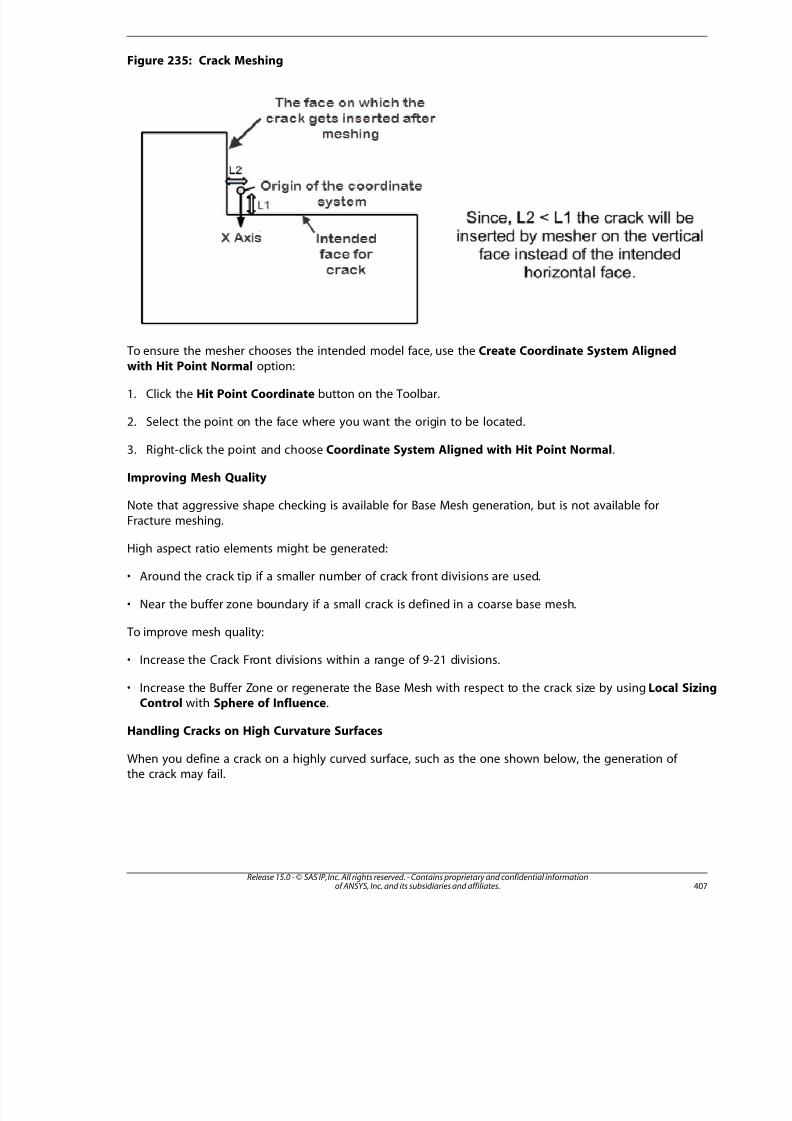
8/10/2019 ANSYS Meshing Users Guide
http://slidepdf.com/reader/full/ansys-meshing-users-guide 415/491
Figure 235: Crack Meshing
To ensure the mesher chooses the intended model face, use the Create Coordinate System Alignedwith Hit Point Normal option:
1. Click the Hit Point Coordinate button on the Toolbar.
2. Select the point on the face where you want the origin to be located.
3. Right-click the point and choose Coordinate System Aligned with Hit Point Normal .
Improving Mesh Quality
Note that aggressive shape checking is available for Base Mesh generation, but is not available for
Fracture meshing.
High aspect ratio elements might be generated:
• Around the crack tip if a smaller number of crack front divisions are used.
• Near the buffer zone boundary if a small crack is defined in a coarse base mesh.
To improve mesh quality:
• Increase the Crack Front divisions within a range of 9-21 divisions.
• Increase the Buffer Zone or regenerate the Base Mesh with respect to the crack size by using Local Sizin
Control with Sphere of Influence.
Handling Cracks on High Curvature Surfaces
When you define a crack on a highly curved surface, such as the one shown below, the generation of the crack may fail.
407Release 15.0 - © SAS IP, Inc. All rights reserved. - Contains proprietary and confidential informationof ANSYS, Inc. and its subsidiaries and affiliates.
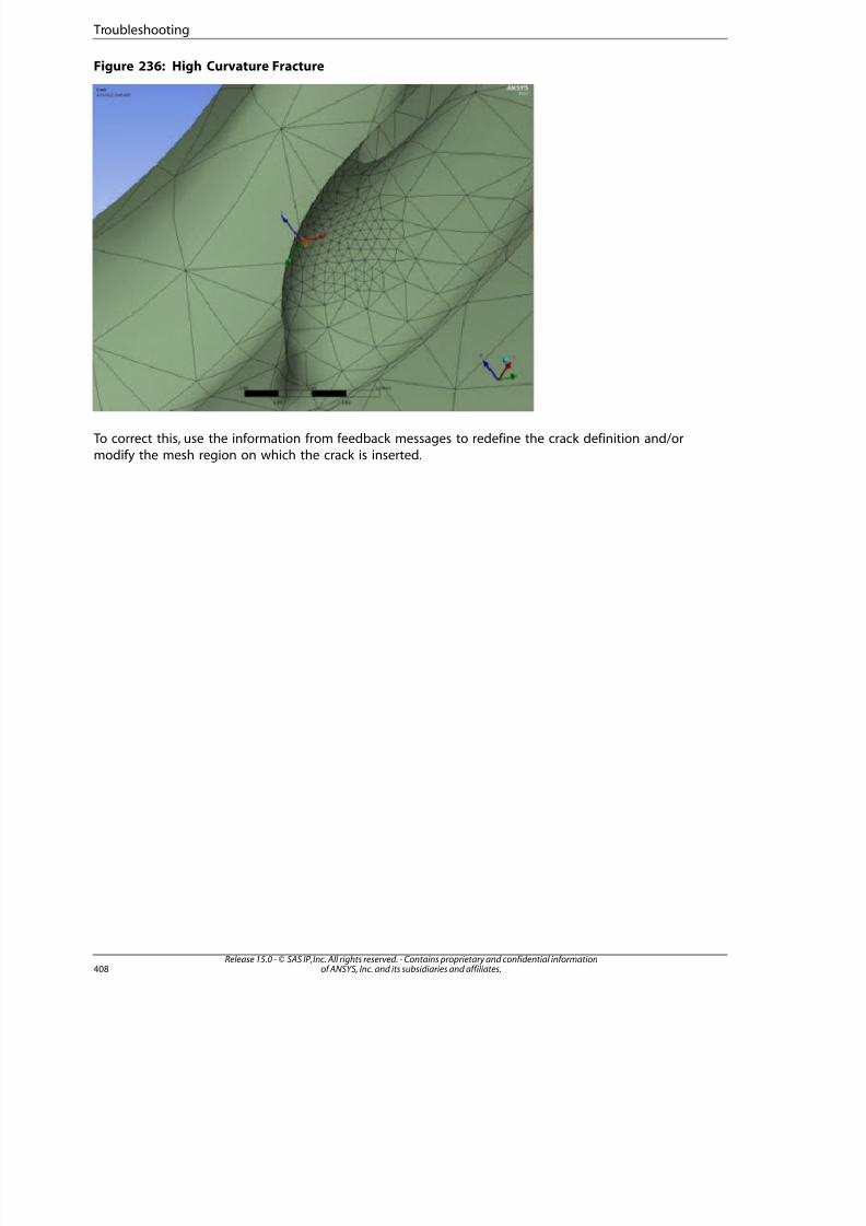
8/10/2019 ANSYS Meshing Users Guide
http://slidepdf.com/reader/full/ansys-meshing-users-guide 416/491
Figure 236: High Curvature Fracture
To correct this, use the information from feedback messages to redefine the crack definition and/ormodify the mesh region on which the crack is inserted.
Release 15.0 - © SAS IP, Inc. All rights reserved. - Contains proprietary and confidential informationof ANSYS, Inc. and its subsidiaries and affiliates.408
Troubleshooting
8/10/2019 ANSYS Meshing Users Guide
http://slidepdf.com/reader/full/ansys-meshing-users-guide 417/491
Meshing: Tutorials
There are various types of tutorials available for the Meshing application. Included within this help arethe following tutorials: Tutorial 1: Can Combustor
Tutorial 2: Single Body Inflation Tutorial 3: Mesh Controls and Methods Tutorial 4: Advanced Size Function
Tutorial 5:Thin Sweep Meshing of a Multibody Part
Tutorial 1: Can Combustor
This tutorial creates a mesh for a can combustor, which can be found in gas turbine engines. The geo-
metry is complex and consists of five separate solid bodies. It will be imported as a complete geometryfrom a Parasolid file.
The diagram below shows the geometry schematically with part of the outer wall cut away.
409Release 15.0 - © SAS IP, Inc. All rights reserved. - Contains proprietary and confidential informationof ANSYS, Inc. and its subsidiaries and affiliates.
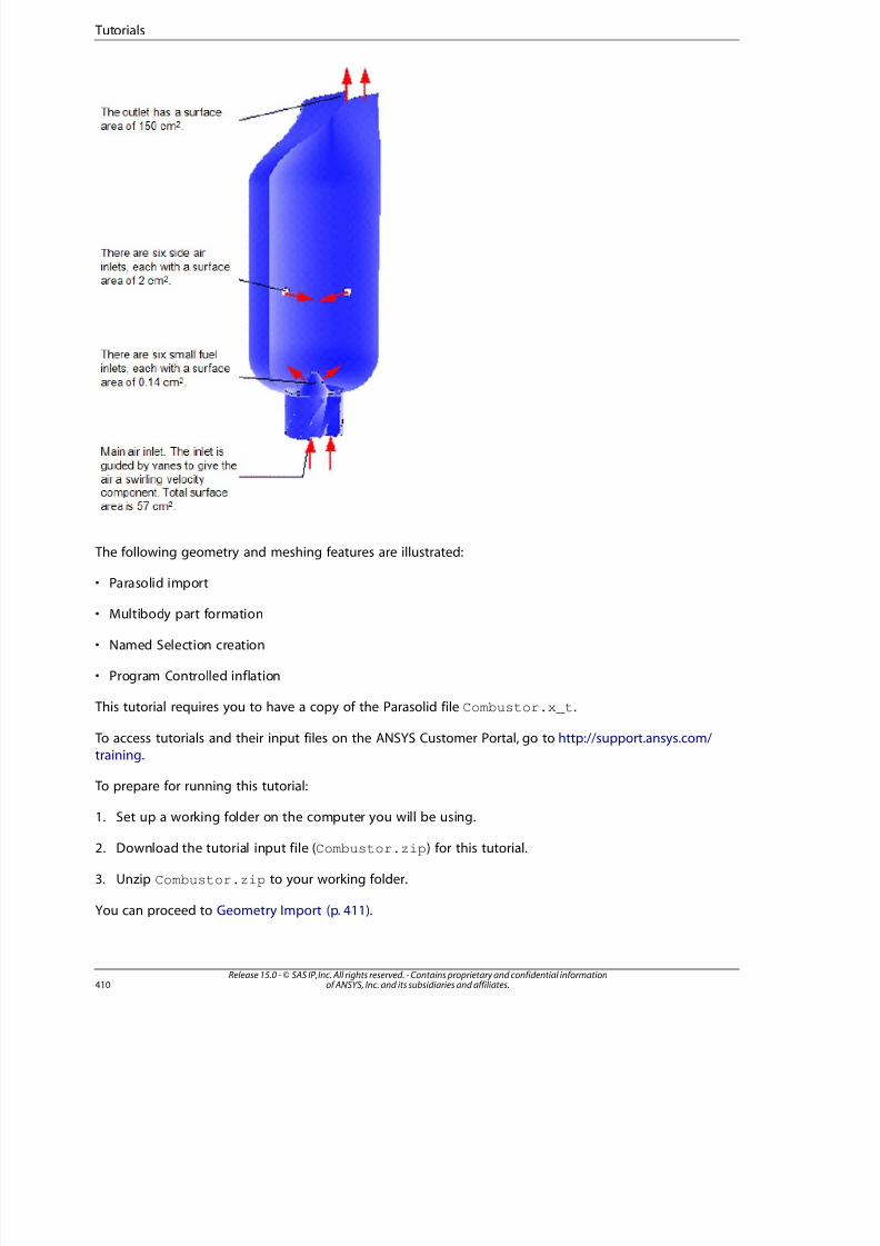
8/10/2019 ANSYS Meshing Users Guide
http://slidepdf.com/reader/full/ansys-meshing-users-guide 418/491
The following geometry and meshing features are illustrated:
• Parasolid import
• Multibody part formation
• Named Selection creation
• Program Controlled inflation
This tutorial requires you to have a copy of the Parasolid file Combustor.x_t.
To access tutorials and their input files on the ANSYS Customer Portal, go to http://support.ansys.com/
training.
To prepare for running this tutorial:
1. Set up a working folder on the computer you will be using.
2. Download the tutorial input file (Combustor.zip) for this tutorial.
3. Unzip Combustor.zip to your working folder.
You can proceed to Geometry Import (p. 411).
Release 15.0 - © SAS IP, Inc. All rights reserved. - Contains proprietary and confidential informationof ANSYS, Inc. and its subsidiaries and affiliates.410
Tutorials
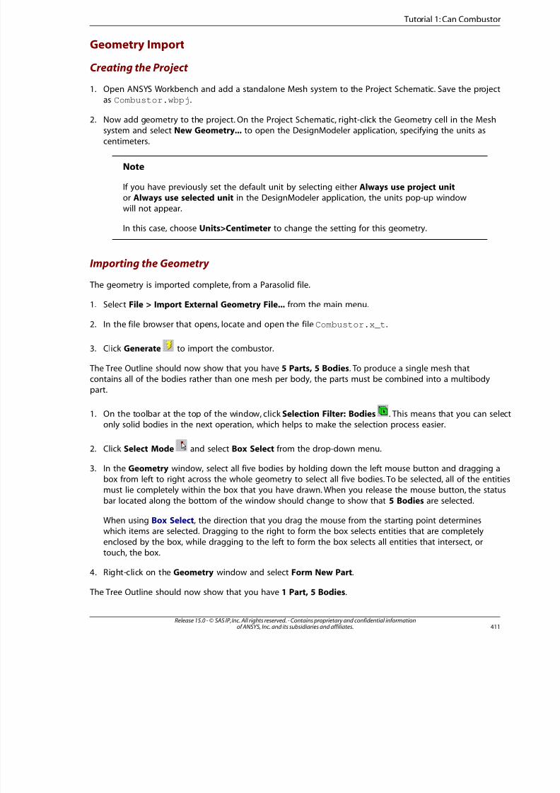
8/10/2019 ANSYS Meshing Users Guide
http://slidepdf.com/reader/full/ansys-meshing-users-guide 419/491
Geometry Import
Creating the Project
1. Open ANSYS Workbench and add a standalone Mesh system to the Project Schematic. Save the projectas Combustor.wbpj.
2. Now add geometry to the project. On the Project Schematic, right-click the Geometry cell in the Meshsystem and select New Geometry... to open the DesignModeler application, specifying the units as
centimeters.
Note
If you have previously set the default unit by selecting either Always use project unitor Always use selected unit in the DesignModeler application, the units pop-up windowwill not appear.
In this case, choose Units>Centimeter to change the setting for this geometry.
Importing the Geometry
The geometry is imported complete, from a Parasolid file.
1. Select File > Import External Geometry File... from the main menu.
2. In the file browser that opens, locate and open the file Combustor.x_t.
3. Click Generate to import the combustor.
The Tree Outline should now show that you have 5 Parts, 5 Bodies. To produce a single mesh thatcontains all of the bodies rather than one mesh per body, the parts must be combined into a multibodypart.
1. On the toolbar at the top of the window, click Selection Filter: Bodies . This means that you can seonly solid bodies in the next operation, which helps to make the selection process easier.
2. Click Select Mode and select Box Select from the drop-down menu.
3. In the Geometry window, select all five bodies by holding down the left mouse button and dragging abox from left to right across the whole geometry to select all five bodies. To be selected, all of the entitmust lie completely within the box that you have drawn. When you release the mouse button, the statu
bar located along the bottom of the window should change to show that 5 Bodies are selected.
When using Box Select, the direction that you drag the mouse from the starting point determineswhich items are selected. Dragging to the right to form the box selects entities that are completely
enclosed by the box, while dragging to the left to form the box selects all entities that intersect, ortouch, the box.
4. Right-click on the Geometry window and select Form New Part.
The Tree Outline should now show that you have 1 Part, 5 Bodies.
41Release 15.0 - © SAS IP, Inc. All rights reserved. - Contains proprietary and confidential informationof ANSYS, Inc. and its subsidiaries and affiliates.
Tutorial 1: Can Combusto

8/10/2019 ANSYS Meshing Users Guide
http://slidepdf.com/reader/full/ansys-meshing-users-guide 420/491
The geometry does not need further modifications. It is now complete. From the DesignModeler applic-ation's main menu, select File > Save Project to save the project and then File > Close DesignModeler
to return to the Project Schematic. Notice the Geometry cell appears in an up-to-date state .
Now that the geometry is complete, you can proceed to Mesh Generation (p. 412).
Mesh Generation
Launching the Meshing Application
On the Project Schematic, right-click the Mesh cell in the Mesh system and select Edit... to launch theMeshing application.
Creating Named Selections
You will create five Named Selections in this tutorial. Detailed instructions are provided for creating the
first Named Selection. Less detailed instructions are provided for creating the subsequent Named Selec-tions, but you should create them in a similar fashion, using additional zoom and/or rotation optionsfrom the toolbar as needed.
1. To create a Named Selection for the fuel inlet, select the six tiny faces on the cone near the bottom of the combustor. The easiest way to select them is as follows:
a. Click over the axes in the bottom right corner of the Geometry window in the position shown in the
figure below. As you move the cursor into this position, the black “-Z”-axis will appear (it is not shownby default). This will put the geometry into a good position for picking the required faces.
b. On the toolbar, click Box Zoom .
c. In the Geometry window, zoom the geometry by holding down the left mouse button and dragginga box across the area where the six tiny faces are located. Then release the mouse button.
d. On the toolbar, click Face .
e. Press and hold the CTRL key while picking the six faces, which are shown in green in the figure below
(the colors in your geometry may differ from those shown in this tutorial).
Release 15.0 - © SAS IP, Inc. All rights reserved. - Contains proprietary and confidential informationof ANSYS, Inc. and its subsidiaries and affiliates.412
Tutorials
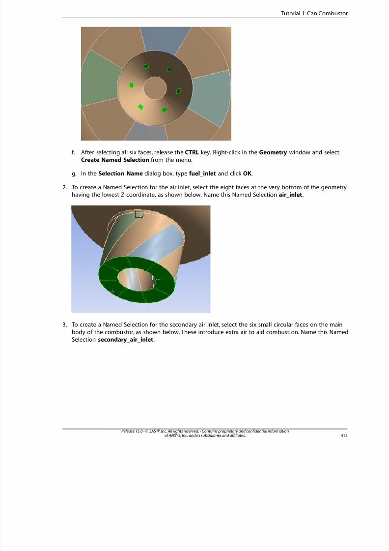
8/10/2019 ANSYS Meshing Users Guide
http://slidepdf.com/reader/full/ansys-meshing-users-guide 421/491
f. After selecting all six faces, release the CTRL key. Right-click in the Geometry window and selectCreate Named Selection from the menu.
g. In the Selection Name dialog box, type fuel_inlet and click OK.
2. To create a Named Selection for the air inlet, select the eight faces at the very bottom of the geometryhaving the lowest Z-coordinate, as shown below. Name this Named Selection air_inlet.
3. To create a Named Selection for the secondary air inlet, select the six small circular faces on the mainbody of the combustor, as shown below. These introduce extra air to aid combustion. Name this NamedSelection secondary_air_inlet.
413Release 15.0 - © SAS IP, Inc. All rights reserved. - Contains proprietary and confidential informationof ANSYS, Inc. and its subsidiaries and affiliates.
Tutorial 1: Can Combusto
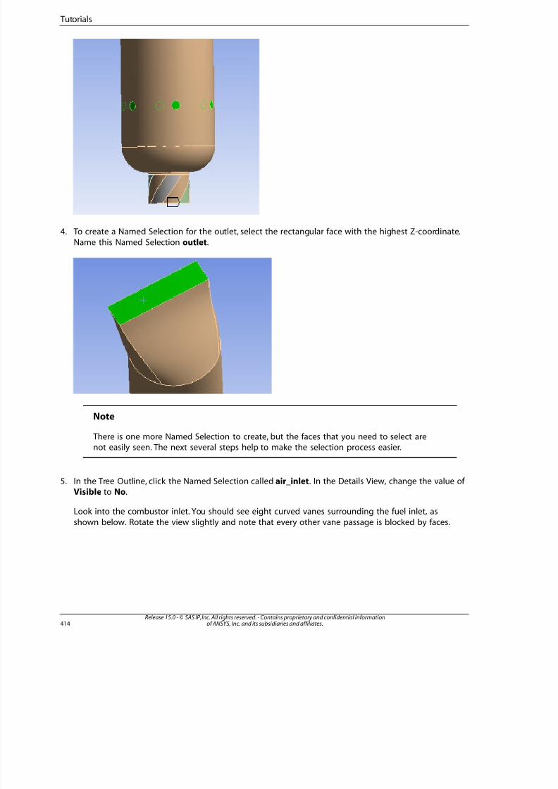
8/10/2019 ANSYS Meshing Users Guide
http://slidepdf.com/reader/full/ansys-meshing-users-guide 422/491
4. To create a Named Selection for the outlet, select the rectangular face with the highest Z-coordinate.
Name this Named Selection outlet.
Note
There is one more Named Selection to create, but the faces that you need to select arenot easily seen. The next several steps help to make the selection process easier.
5. In the Tree Outline, click the Named Selection called air_inlet. In the Details View, change the value of
Visible to No.
Look into the combustor inlet. You should see eight curved vanes surrounding the fuel inlet, as
shown below. Rotate the view slightly and note that every other vane passage is blocked by faces.
Release 15.0 - © SAS IP, Inc. All rights reserved. - Contains proprietary and confidential informationof ANSYS, Inc. and its subsidiaries and affiliates.414
Tutorials
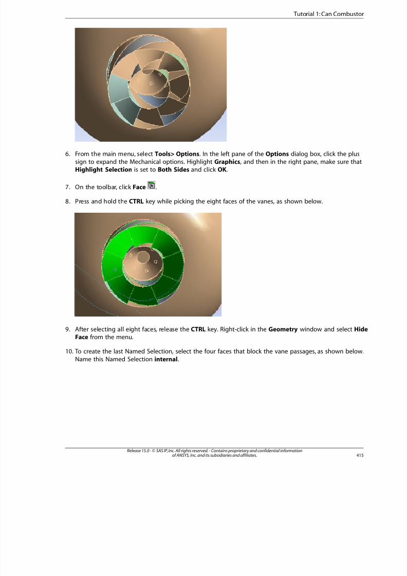
8/10/2019 ANSYS Meshing Users Guide
http://slidepdf.com/reader/full/ansys-meshing-users-guide 423/491

8/10/2019 ANSYS Meshing Users Guide
http://slidepdf.com/reader/full/ansys-meshing-users-guide 424/491
Note
You are done creating Named Selections. The next several steps toggle visibility of allfaces back on.
11. In the Tree Outline, click the Named Selection called air_inlet. In the Details View, change the value of Visible to Yes.
12. Right-click in the Geometry window and select Show Hidden Face(s) from the menu.
Setting Up the Mesh
This is a complex geometry which will be used to run a simulation with complex physics. To keep thecomputational time down for the purposes of the tutorial, the default sizing settings will be retained
and a very coarse mesh will be generated. If you wanted to get accurate results for the geometry, amuch finer mesh and a much longer solution time would be required.
1. In the Tree Outline, click the Mesh object.
2. In the Details View, set Physics Preference to CFD and Solver Preference to CFX.
3. In the Details View, click to expand the Sizing group of controls and notice the default sizing settings.
Setting Up Inflation
It is a good idea to put inflation on the walls.
1. In the Details View, click to expand the Inflation group of controls.
2. Set Use Automatic Inflation to Program Controlled.
As a result of this setting, all faces in the model are selected to be inflation boundaries, with a few ex-ceptions. For the purposes of this tutorial, the important exception is Named Selections—the faces in
Named Selections will not be selected to be inflation boundaries.
Generating the Mesh
Finally, you can generate the mesh by right-clicking Mesh in the Tree Outline and selecting GenerateMesh. After a few moments, the meshed model appears in the Geometry window, as shown below.
Release 15.0 - © SAS IP, Inc. All rights reserved. - Contains proprietary and confidential informationof ANSYS, Inc. and its subsidiaries and affiliates.416
Tutorials
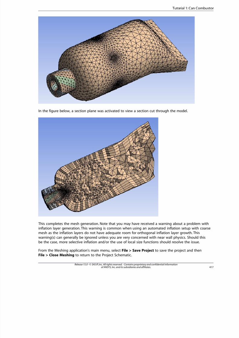
8/10/2019 ANSYS Meshing Users Guide
http://slidepdf.com/reader/full/ansys-meshing-users-guide 425/491
In the figure below, a section plane was activated to view a section cut through the model.
This completes the mesh generation. Note that you may have received a warning about a problem withinflation layer generation. This warning is common when using an automated inflation setup with coarsemesh as the inflation layers do not have adequate room for orthogonal inflation layer growth. This
warning(s) can generally be ignored unless you are very concerned with near wall physics. Should thisbe the case, more selective inflation and/or the use of local size functions should resolve the issue.
From the Meshing application's main menu, select File > Save Project to save the project and then
File > Close Meshing to return to the Project Schematic.
417Release 15.0 - © SAS IP, Inc. All rights reserved. - Contains proprietary and confidential informationof ANSYS, Inc. and its subsidiaries and affiliates.
Tutorial 1: Can Combusto
8/10/2019 ANSYS Meshing Users Guide
http://slidepdf.com/reader/full/ansys-meshing-users-guide 426/491
You can exit ANSYS Workbench by selecting File > Exit from the main menu.
Tutorial 2: Single Body Inflation
This tutorial demonstrates various ways to apply single body inflation. The 3D inflation capabilityprovided by the Meshing application is mainly used in CFD/Fluids meshing. It provides high quality
mesh generation close to wall boundaries to resolve changes in physical properties.
Essentially, there are two methods for applying inflation: globally, using Named Selections; and locally,by scoping an inflation method. This tutorial covers using these methods along with various other settings
for defining inflation on a single body.
The following topics are covered:
• Comparing two Collision Avoidance (p. 90) settings (Layer Compression and Stair Stepping), whichdetermine the approach that is to be taken in areas of proximity
• Previewing inflation, which can be used to examine proximity handling, determine the quality of inflationlayers, and detect potential quality issues
• Creating a new Named Selection, and automatically applying inflation to all the faces in it
• Scoping inflation to a body and selecting a Named Selection as the inflation boundary
• Comparing three Inflation Option (p. 83) settings (Smooth Transition, Total Thickness, and Last AspectRatio), which determine the heights of the inflation layers
• Changing Solver Preference (p. 67) and how its value affects default inflation behaviors
This tutorial requires you to have a copy of the ANSYS Workbench project file newquart.wbpj and
the project folder newquart_files and its contents.
To access tutorials and their input files on the ANSYS Customer Portal, go to http://support.ansys.com/training.
To prepare for running this tutorial:
1. Set up a working folder on the computer you will be using.
2. Download the tutorial input file (Newquart.zip) for this tutorial.
3. Unzip Newquart.zip to your working folder.
You can proceed to Tutorial Setup (p. 418).
Tutorial Setup
Opening the Project
1. Open ANSYS Workbench.
2. Select File > Open... from the main menu.
3. In the file browser that opens, locate and open the file newquart.wbpj.
Release 15.0 - © SAS IP, Inc. All rights reserved. - Contains proprietary and confidential informationof ANSYS, Inc. and its subsidiaries and affiliates.418
Tutorials

8/10/2019 ANSYS Meshing Users Guide
http://slidepdf.com/reader/full/ansys-meshing-users-guide 427/491
Now that the tutorial is set up, you can proceed to Mesh Generation (p. 419).
Mesh Generation
Launching the Meshing Application
On the Project Schematic, right-click the Mesh cell in the Mesh system and select Edit... to launch theMeshing application.
Setting the Unit System
On the main menu, click Units and select Metric (mm, kg, N, s, mV, mA).
Program Controlled Inflation Using the Fluent Solver
This part of the tutorial demonstrates the use of Program Controlled (p. 81) inflation with the Fluentsolver. Notice that three Named Selections are defined already: Symmetry, Inlet, and Outlet. You willcreate a fourth later in this tutorial.
1. In the Tree Outline, click the Mesh object.
In the Details View, notice that Solver Preference (p. 67) is set to Fluent.
2. Click to expand the Sizing group of controls and change Curvature Normal Angle (p. 72) to 12.
3. Click to expand the Inflation group of controls.
Notice that Program Controlled (p. 81) and Smooth Transition are selected and Transition Ra-tio (p. 85) is set to 0.272 by default.
With Program Controlled (p. 81) inflation, inflation will be added to all external faces for which aNamed Selection has not been defined.
When Solver Preference (p. 67) is Fluent, the default Transition Ratio (p. 85) is 0.272 because the
solver uses a cell-centered scheme. This is in contrast to the CFX Solver Preference (p. 67), whichis covered later in this tutorial.
4. Change Maximum Layers (p. 85) to 5.
5. In the Tree Outline, right-click Mesh and select Preview > Inflation. Previewing inflation helps to
identify possible problems with inflation before generating a full mesh.
After a few moments, a preview of the inflation layers appears in the Geometry window, as shownbelow.
419Release 15.0 - © SAS IP, Inc. All rights reserved. - Contains proprietary and confidential informationof ANSYS, Inc. and its subsidiaries and affiliates.
Tutorial 2: Single Body Inflation
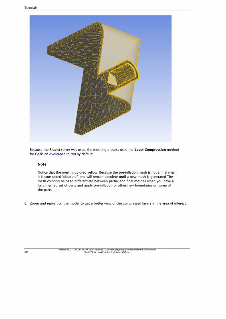
8/10/2019 ANSYS Meshing Users Guide
http://slidepdf.com/reader/full/ansys-meshing-users-guide 428/491
Because the Fluent solver was used, the meshing process used the Layer Compression methodfor Collision Avoidance (p. 90) by default.
Note
Notice that the mesh is colored yellow. Because the pre-inflation mesh is not a final mesh,it is considered “obsolete," and will remain obsolete until a new mesh is generated. The
mesh coloring helps to differentiate between partial and final meshes when you have afully meshed set of parts and apply pre-inflation or other new boundaries on some of the parts.
6. Zoom and reposition the model to get a better view of the compressed layers in the area of interest.
Release 15.0 - © SAS IP, Inc. All rights reserved. - Contains proprietary and confidential informationof ANSYS, Inc. and its subsidiaries and affiliates.420
Tutorials
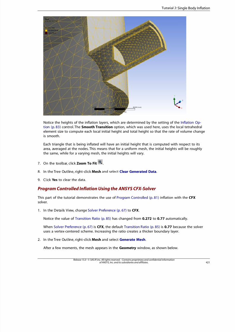
8/10/2019 ANSYS Meshing Users Guide
http://slidepdf.com/reader/full/ansys-meshing-users-guide 429/491
Notice the heights of the inflation layers, which are determined by the setting of the Inflation Op-tion (p. 83) control. The Smooth Transition option, which was used here, uses the local tetrahedralelement size to compute each local initial height and total height so that the rate of volume change
is smooth.
Each triangle that is being inflated will have an initial height that is computed with respect to itsarea, averaged at the nodes. This means that for a uniform mesh, the initial heights will be roughly
the same, while for a varying mesh, the initial heights will vary.
7. On the toolbar, click Zoom To Fit .
8. In the Tree Outline, right-click Mesh and select Clear Generated Data.
9. Click Yes to clear the data.
Program Controlled Inflation Using the ANSYS CFX-Solver
This part of the tutorial demonstrates the use of Program Controlled (p. 81) inflation with the CFXsolver.
1. In the Details View, change Solver Preference (p. 67) to CFX.
Notice the value of Transition Ratio (p. 85) has changed from 0.272 to 0.77 automatically.
When Solver Preference (p. 67) is CFX, the default Transition Ratio (p. 85) is 0.77 because the solveruses a vertex-centered scheme. Increasing the ratio creates a thicker boundary layer.
2. In the Tree Outline, right-click Mesh and select Generate Mesh.
After a few moments, the mesh appears in the Geometry window, as shown below.
42Release 15.0 - © SAS IP, Inc. All rights reserved. - Contains proprietary and confidential informationof ANSYS, Inc. and its subsidiaries and affiliates.
Tutorial 2: Single Body Inflation
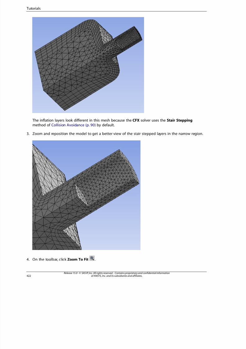
8/10/2019 ANSYS Meshing Users Guide
http://slidepdf.com/reader/full/ansys-meshing-users-guide 430/491
The inflation layers look different in this mesh because the CFX solver uses the Stair Steppingmethod of Collision Avoidance (p. 90) by default.
3. Zoom and reposition the model to get a better view of the stair stepped layers in the narrow region.
4. On the toolbar, click Zoom To Fit .
Release 15.0 - © SAS IP, Inc. All rights reserved. - Contains proprietary and confidential informationof ANSYS, Inc. and its subsidiaries and affiliates.422
Tutorials
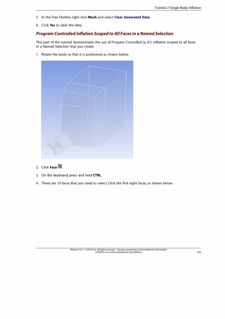
8/10/2019 ANSYS Meshing Users Guide
http://slidepdf.com/reader/full/ansys-meshing-users-guide 431/491
5. In the Tree Outline, right-click Mesh and select Clear Generated Data.
6. Click Yes to clear the data.
Program Controlled Inflation Scoped to All Faces in a Named Selection
This part of the tutorial demonstrates the use of Program Controlled (p. 81) inflation scoped to all facesin a Named Selection that you create.
1. Rotate the body so that it is positioned as shown below.
2. Click Face .
3. On the keyboard, press and hold CTRL.
4. There are 10 faces that you need to select. Click the first eight faces, as shown below.
423Release 15.0 - © SAS IP, Inc. All rights reserved. - Contains proprietary and confidential informationof ANSYS, Inc. and its subsidiaries and affiliates.
Tutorial 2: Single Body Inflation
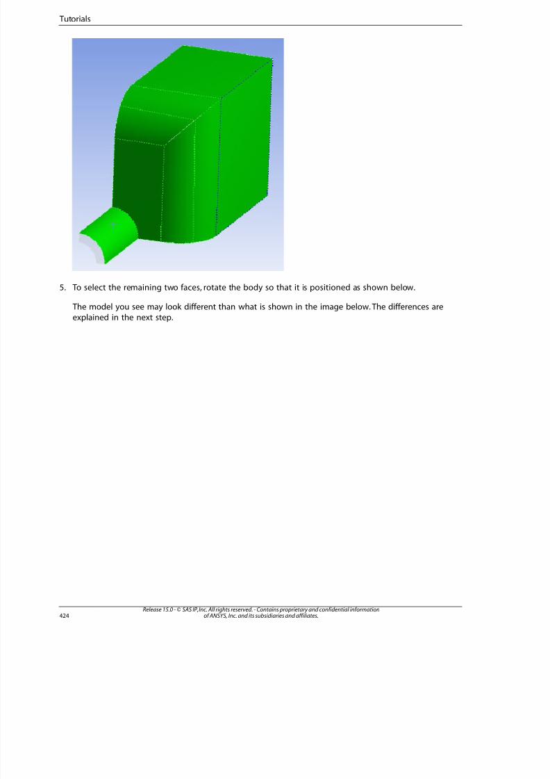
8/10/2019 ANSYS Meshing Users Guide
http://slidepdf.com/reader/full/ansys-meshing-users-guide 432/491
5. To select the remaining two faces, rotate the body so that it is positioned as shown below.
The model you see may look different than what is shown in the image below. The differences are
explained in the next step.
Release 15.0 - © SAS IP, Inc. All rights reserved. - Contains proprietary and confidential informationof ANSYS, Inc. and its subsidiaries and affiliates.424
Tutorials
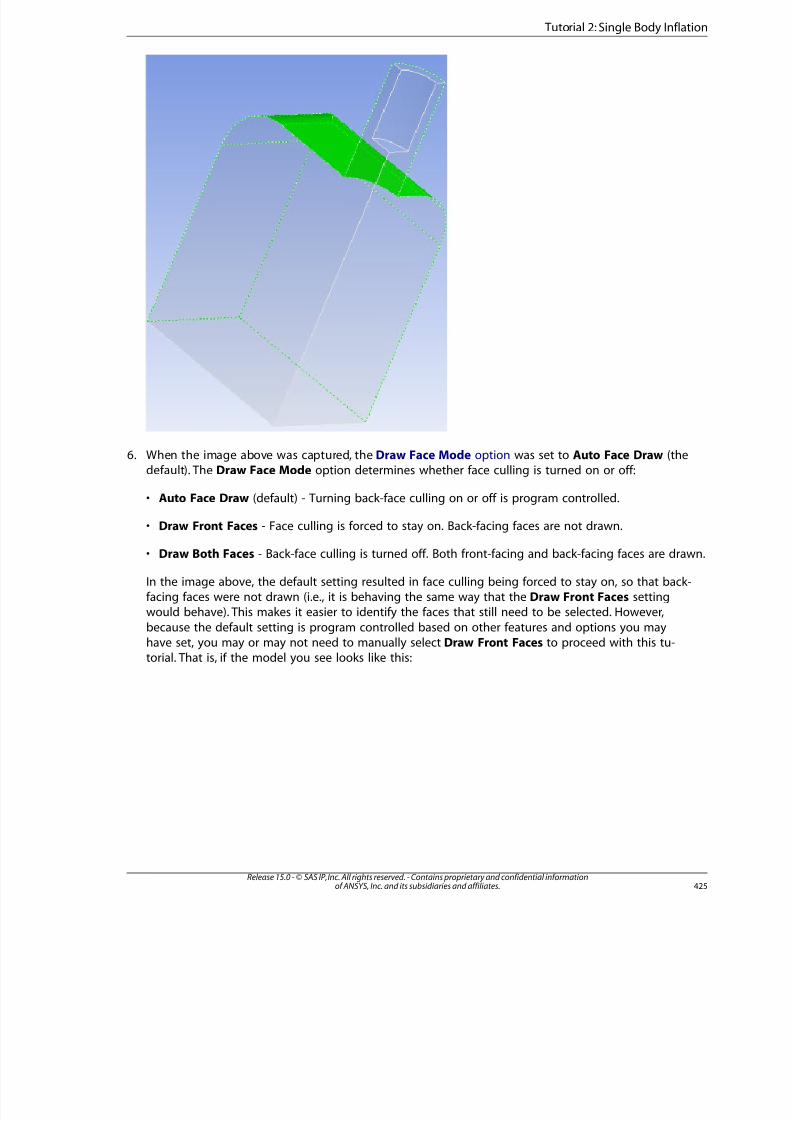
8/10/2019 ANSYS Meshing Users Guide
http://slidepdf.com/reader/full/ansys-meshing-users-guide 433/491
6. When the image above was captured, the Draw Face Mode option was set to Auto Face Draw (thedefault). The Draw Face Mode option determines whether face culling is turned on or off:
• Auto Face Draw (default) - Turning back-face culling on or off is program controlled.
• Draw Front Faces - Face culling is forced to stay on. Back-facing faces are not drawn.
• Draw Both Faces - Back-face culling is turned off. Both front-facing and back-facing faces are drawn.
In the image above, the default setting resulted in face culling being forced to stay on, so that back-facing faces were not drawn (i.e., it is behaving the same way that the Draw Front Faces settingwould behave). This makes it easier to identify the faces that still need to be selected. However,
because the default setting is program controlled based on other features and options you mayhave set, you may or may not need to manually select Draw Front Faces to proceed with this tu-torial. That is, if the model you see looks like this:
425Release 15.0 - © SAS IP, Inc. All rights reserved. - Contains proprietary and confidential informationof ANSYS, Inc. and its subsidiaries and affiliates.
Tutorial 2: Single Body Inflation
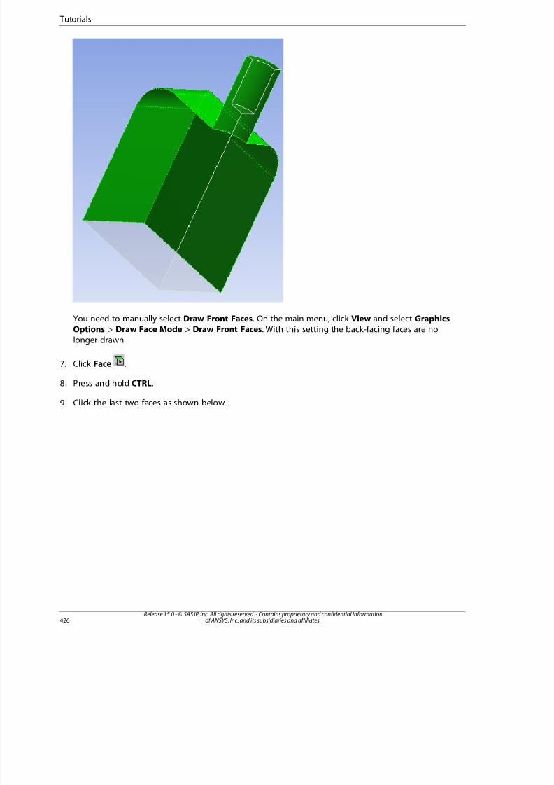
8/10/2019 ANSYS Meshing Users Guide
http://slidepdf.com/reader/full/ansys-meshing-users-guide 434/491
You need to manually select Draw Front Faces. On the main menu, click View and select GraphicsOptions > Draw Face Mode > Draw Front Faces. With this setting the back-facing faces are no
longer drawn.
7. Click Face .
8. Press and hold CTRL.
9. Click the last two faces as shown below.
Release 15.0 - © SAS IP, Inc. All rights reserved. - Contains proprietary and confidential informationof ANSYS, Inc. and its subsidiaries and affiliates.426
Tutorials
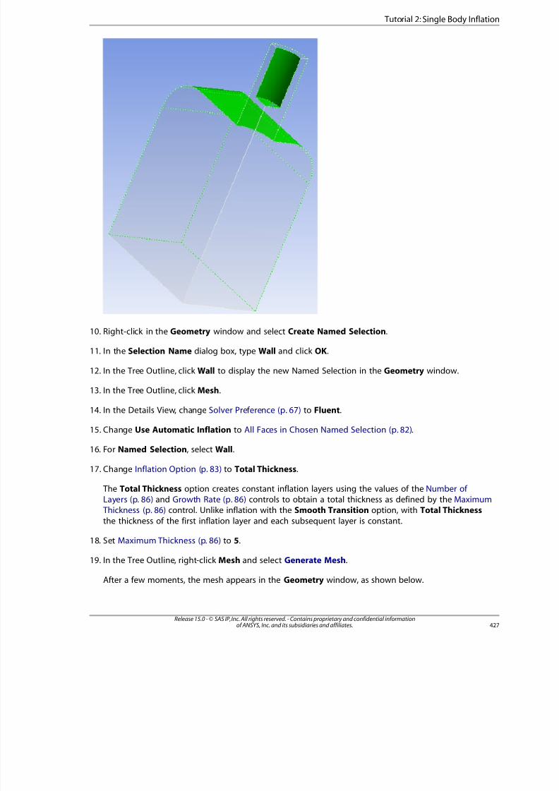
8/10/2019 ANSYS Meshing Users Guide
http://slidepdf.com/reader/full/ansys-meshing-users-guide 435/491
10. Right-click in the Geometry window and select Create Named Selection.
11. In the Selection Name dialog box, type Wall and click OK.
12. In the Tree Outline, click Wall to display the new Named Selection in the Geometry window.
13. In the Tree Outline, click Mesh.
14. In the Details View, change Solver Preference (p. 67) to Fluent.
15. Change Use Automatic Inflation to All Faces in Chosen Named Selection (p. 82).
16. For Named Selection, select Wall.
17. Change Inflation Option (p. 83) to Total Thickness.
The Total Thickness option creates constant inflation layers using the values of the Number of
Layers (p. 86) and Growth Rate (p. 86) controls to obtain a total thickness as defined by the Maximum Thickness (p. 86) control. Unlike inflation with the Smooth Transition option, with Total Thickness
the thickness of the first inflation layer and each subsequent layer is constant.
18. Set Maximum Thickness (p. 86) to 5.
19. In the Tree Outline, right-click Mesh and select Generate Mesh.
After a few moments, the mesh appears in the Geometry window, as shown below.
427Release 15.0 - © SAS IP, Inc. All rights reserved. - Contains proprietary and confidential informationof ANSYS, Inc. and its subsidiaries and affiliates.
Tutorial 2: Single Body Inflation
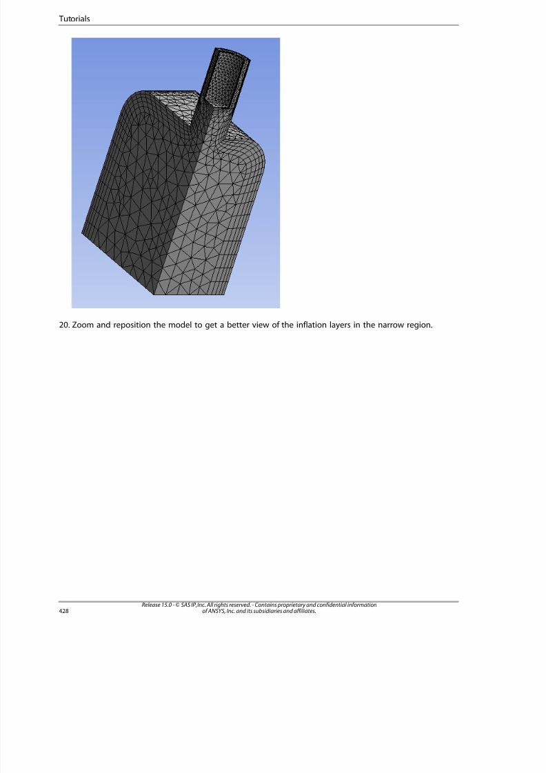
8/10/2019 ANSYS Meshing Users Guide
http://slidepdf.com/reader/full/ansys-meshing-users-guide 436/491
20. Zoom and reposition the model to get a better view of the inflation layers in the narrow region.
Release 15.0 - © SAS IP, Inc. All rights reserved. - Contains proprietary and confidential informationof ANSYS, Inc. and its subsidiaries and affiliates.428
Tutorials
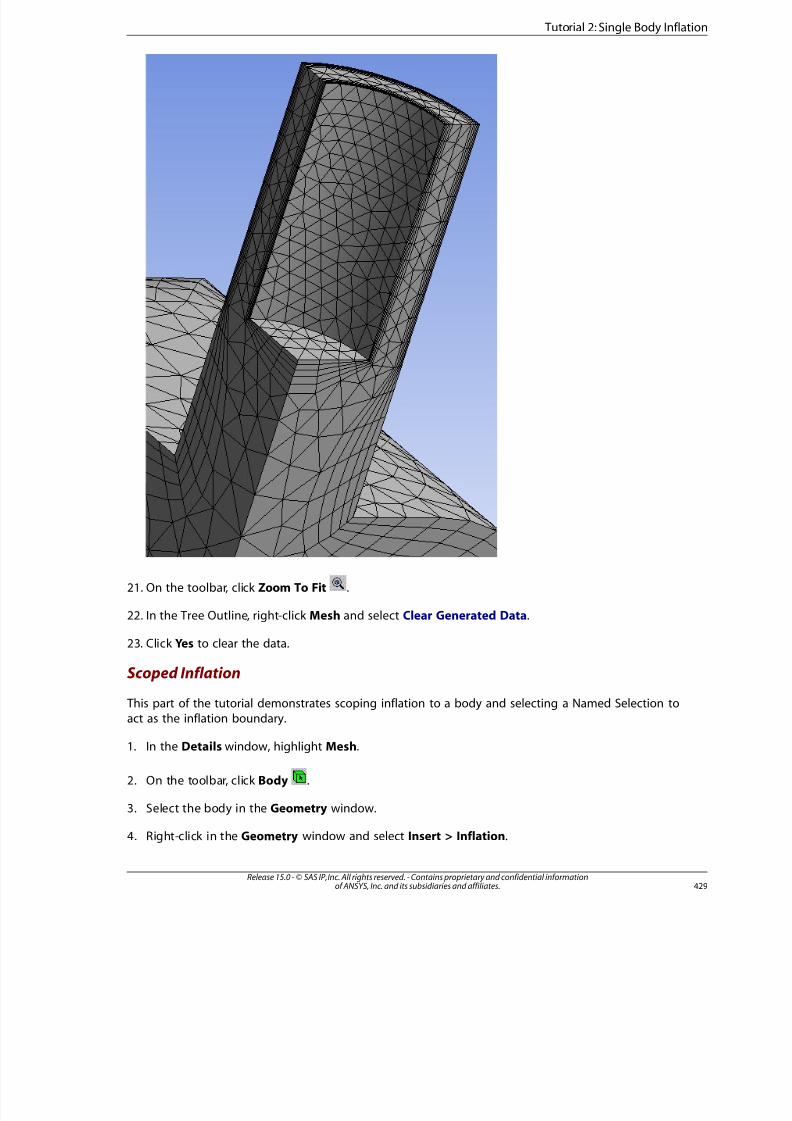
8/10/2019 ANSYS Meshing Users Guide
http://slidepdf.com/reader/full/ansys-meshing-users-guide 437/491

8/10/2019 ANSYS Meshing Users Guide
http://slidepdf.com/reader/full/ansys-meshing-users-guide 438/491
In the Details View, notice that inflation will be scoped to 1 Body.
5. In the Details View, set Boundary Scoping Method to Named Selections.
6. From the Boundary drop-down menu, select Wall by highlighting it in the drop-down menu and thenpressing Enter.
7. Change Inflation Option (p. 83) to Last Aspect Ratio.
The Last Aspect Ratio option creates inflation layers using the values of the First Layer Height (p. 86),Maximum Layers (p. 85), and Aspect Ratio (Base/Height) (p. 86) controls. With this option, the heightsof the inflation layers are determined by the aspect ratio of the inflations that are extruded from
the inflation base. The aspect ratio is defined as the ratio of the local inflation base size to the inflationlayer height.
8. Set First Layer Height (p. 86) to 0.5.
9. You are now finished setting the scoped (local) inflation controls. In the Tree Outline, click Mesh to returnto the global inflation controls.
10. In the Details View, change Solver Preference (p. 67) to CFX.
11. Change Use Automatic Inflation to None (p. 80).
12. In the Tree Outline, right-click Mesh and select Preview > Inflation.
After a few moments, the mesh appears in the Geometry window, as shown below.
Release 15.0 - © SAS IP, Inc. All rights reserved. - Contains proprietary and confidential informationof ANSYS, Inc. and its subsidiaries and affiliates.430
Tutorials
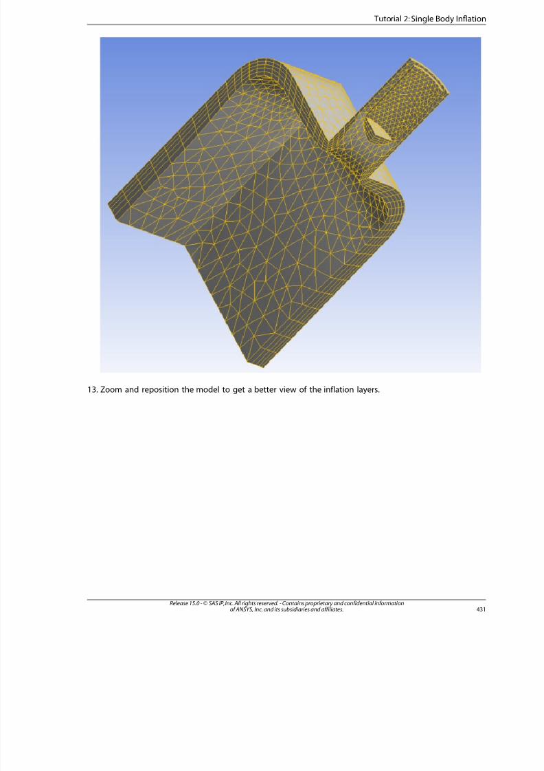
8/10/2019 ANSYS Meshing Users Guide
http://slidepdf.com/reader/full/ansys-meshing-users-guide 439/491
13. Zoom and reposition the model to get a better view of the inflation layers.
43Release 15.0 - © SAS IP, Inc. All rights reserved. - Contains proprietary and confidential informationof ANSYS, Inc. and its subsidiaries and affiliates.
Tutorial 2: Single Body Inflation
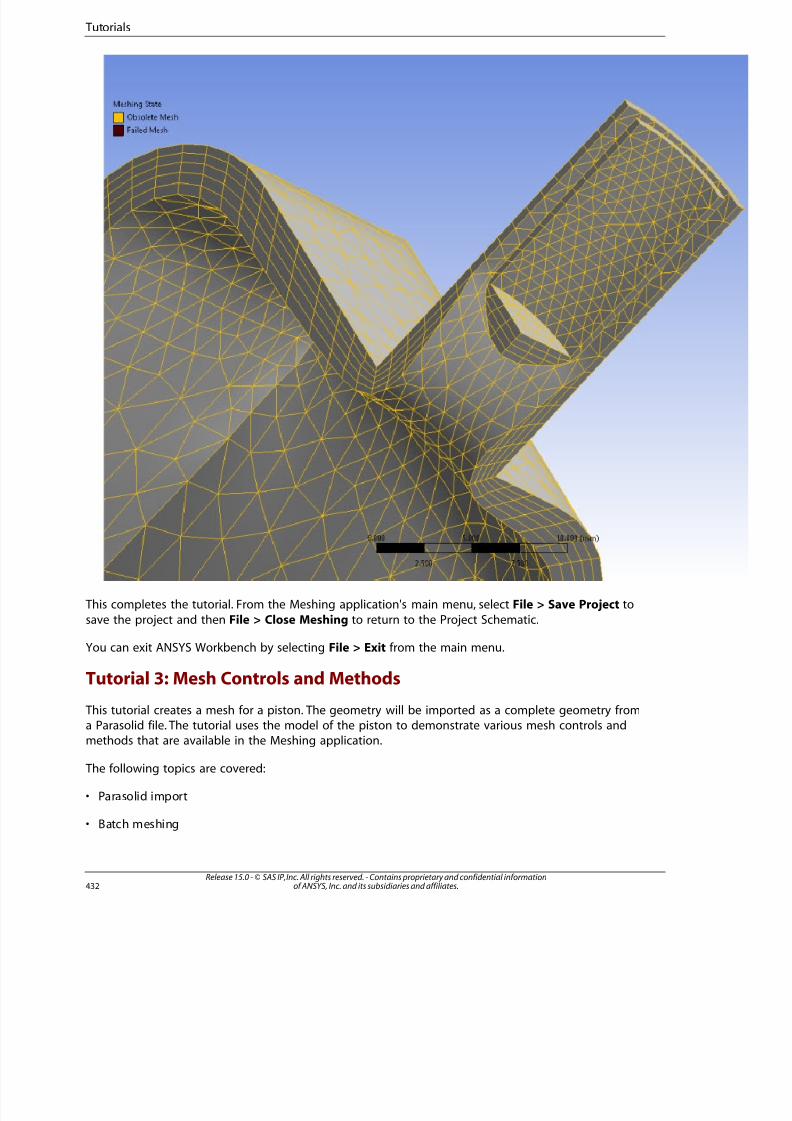
8/10/2019 ANSYS Meshing Users Guide
http://slidepdf.com/reader/full/ansys-meshing-users-guide 440/491
This completes the tutorial. From the Meshing application's main menu, select File > Save Project to
save the project and then File > Close Meshing to return to the Project Schematic.
You can exit ANSYS Workbench by selecting File > Exit from the main menu.
Tutorial 3: Mesh Controls and Methods
This tutorial creates a mesh for a piston. The geometry will be imported as a complete geometry froma Parasolid file. The tutorial uses the model of the piston to demonstrate various mesh controls andmethods that are available in the Meshing application.
The following topics are covered:
• Parasolid import
• Batch meshing
Release 15.0 - © SAS IP, Inc. All rights reserved. - Contains proprietary and confidential informationof ANSYS, Inc. and its subsidiaries and affiliates.432
Tutorials
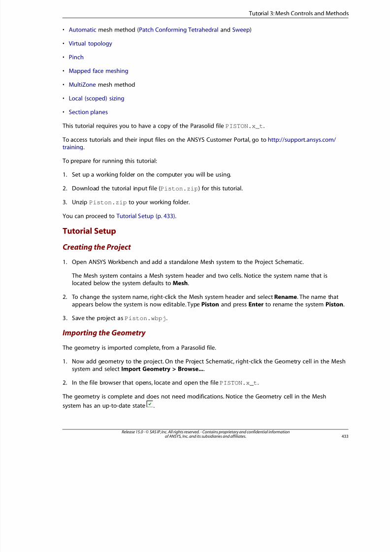
8/10/2019 ANSYS Meshing Users Guide
http://slidepdf.com/reader/full/ansys-meshing-users-guide 441/491
• Automatic mesh method (Patch Conforming Tetrahedral and Sweep)
• Virtual topology
• Pinch
• Mapped face meshing
• MultiZone mesh method
• Local (scoped) sizing
• Section planes
This tutorial requires you to have a copy of the Parasolid file PISTON.x_t.
To access tutorials and their input files on the ANSYS Customer Portal, go to http://support.ansys.com/training.
To prepare for running this tutorial:
1. Set up a working folder on the computer you will be using.
2. Download the tutorial input file (Piston.zip) for this tutorial.
3. Unzip Piston.zip to your working folder.
You can proceed to Tutorial Setup (p. 433).
Tutorial Setup
Creating the Project
1. Open ANSYS Workbench and add a standalone Mesh system to the Project Schematic.
The Mesh system contains a Mesh system header and two cells. Notice the system name that islocated below the system defaults to Mesh.
2. To change the system name, right-click the Mesh system header and select Rename. The name thatappears below the system is now editable. Type Piston and press Enter to rename the system Piston.
3. Save the project as Piston.wbpj.
Importing the Geometry
The geometry is imported complete, from a Parasolid file.
1. Now add geometry to the project. On the Project Schematic, right-click the Geometry cell in the Mesh
system and select Import Geometry > Browse....
2. In the file browser that opens, locate and open the file PISTON.x_t.
The geometry is complete and does not need modifications. Notice the Geometry cell in the Mesh
system has an up-to-date state .
433Release 15.0 - © SAS IP, Inc. All rights reserved. - Contains proprietary and confidential informationof ANSYS, Inc. and its subsidiaries and affiliates.
Tutorial 3: Mesh Controls and Methods

8/10/2019 ANSYS Meshing Users Guide
http://slidepdf.com/reader/full/ansys-meshing-users-guide 442/491
Now that the tutorial is set up, you can proceed to Mesh Generation (p. 434).
Mesh Generation
Running the Meshing Application in Batch Mode
Meshing in batch requires less RAM.
1. On the Project Schematic, right-click the Mesh cell in the Mesh system and select Update to mesh the
geometry in batch mode.
After a short wait, the meshing process is complete. Notice the Mesh cell in the Mesh system has
an up-to-date state .
Launching the Meshing Application
Launch the Meshing application to view the mesh and define mesh controls.
1. Right-click the Mesh cell in the Mesh system and select Edit....
2. When the Meshing application opens, click the Mesh object in the Tree Outline to view the meshed
model in the Geometry window as shown below.
Since no mesh controls have been set, the Automatic mesh method was used by default. When theAutomatic method is used, bodies are swept if possible, and the remaining bodies are meshed withthe Patch Conforming Tetrahedral mesh method.
Release 15.0 - © SAS IP, Inc. All rights reserved. - Contains proprietary and confidential informationof ANSYS, Inc. and its subsidiaries and affiliates.434
Tutorials

8/10/2019 ANSYS Meshing Users Guide
http://slidepdf.com/reader/full/ansys-meshing-users-guide 443/491
Setting the Unit System
On the main menu, click Units and select Metric (m, kg, N, s, V, A).
Showing Sweepable Bodies
This part of the tutorial demonstrates how to view the bodies that were swept. As an alternative, you
can view sweepable bodies prior to meshing.
1. In the Tree Outline, right-click Mesh and select Show > Sweepable Bodies.
The sweepable bodies are highlighted in the Geometry window.
2. To hide all non-sweepable bodies for a better view of the sweepable bodies, right-click on the Geometwindow and select Hide All Other Bodies.
Only the bodies that were meshed with the sweep method appear in the Geometry window, asshown below.
3. Right-click on the Geometry window and select Show All Bodies.
All bodies re-appear in the Geometry window.
4. In the Tree Outline, right-click Mesh and select Show > Sweepable Bodies again.
5. Right-click on the Geometry window and select Hide Body.
Now only the sweepable bodies are hidden. Those bodies that remain in the Geometry windowwere meshed with the Patch Conforming Tetrahedral method.
Creating Virtual Cells Manually
Each surface patch is respected when the Patch Conforming Tetrahedral mesh method is used. Thispart of the tutorial demonstrates how to define virtual topology to merge patches and thus not constrain
the mesh to conform to the patches.
1. Rotate and zoom the geometry so that the model is positioned as shown below. Notice how the meshconforms to the small patches.
435Release 15.0 - © SAS IP, Inc. All rights reserved. - Contains proprietary and confidential informationof ANSYS, Inc. and its subsidiaries and affiliates.
Tutorial 3: Mesh Controls and Methods
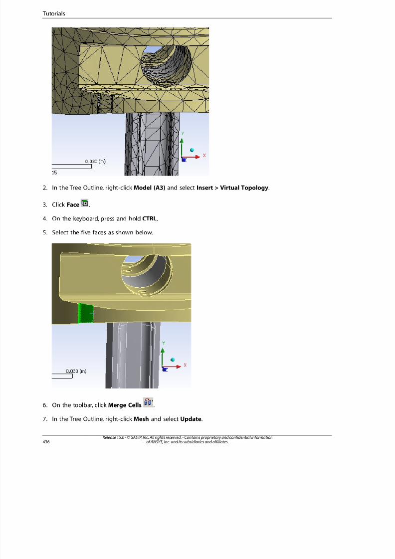
8/10/2019 ANSYS Meshing Users Guide
http://slidepdf.com/reader/full/ansys-meshing-users-guide 444/491
2. In the Tree Outline, right-click Model (A3) and select Insert > Virtual Topology.
3. Click Face .
4. On the keyboard, press and hold CTRL.
5. Select the five faces as shown below.
6. On the toolbar, click Merge Cells .
7. In the Tree Outline, right-click Mesh and select Update.
Release 15.0 - © SAS IP, Inc. All rights reserved. - Contains proprietary and confidential informationof ANSYS, Inc. and its subsidiaries and affiliates.436
Tutorials
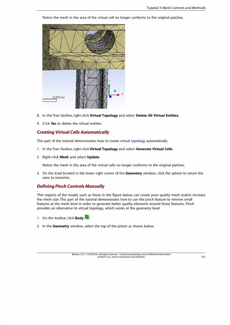
8/10/2019 ANSYS Meshing Users Guide
http://slidepdf.com/reader/full/ansys-meshing-users-guide 445/491
Notice the mesh in the area of the virtual cell no longer conforms to the original patches.
8. In the Tree Outline, right-click Virtual Topology and select Delete All Virtual Entities.
9. Click Yes to delete the virtual entities.
Creating Virtual Cells Automatically
This part of the tutorial demonstrates how to create virtual topology automatically.
1. In the Tree Outline, right-click Virtual Topology and select Generate Virtual Cells.
2. Right-click Mesh and select Update.
Notice the mesh in the area of the virtual cells no longer conforms to the original patches.
3. On the triad located in the lower right corner of the Geometry window, click the sphere to return theview to isometric.
Defining Pinch Controls Manually
Thin regions of the model, such as those in the figure below, can create poor quality mesh and/or increase
the mesh size. This part of the tutorial demonstrates how to use the pinch feature to remove small
features at the mesh level in order to generate better quality elements around those features. Pinchprovides an alternative to virtual topology, which works at the geometry level.
1. On the toolbar, click Body .
2. In the Geometry window, select the top of the piston as shown below.
437Release 15.0 - © SAS IP, Inc. All rights reserved. - Contains proprietary and confidential informationof ANSYS, Inc. and its subsidiaries and affiliates.
Tutorial 3: Mesh Controls and Methods
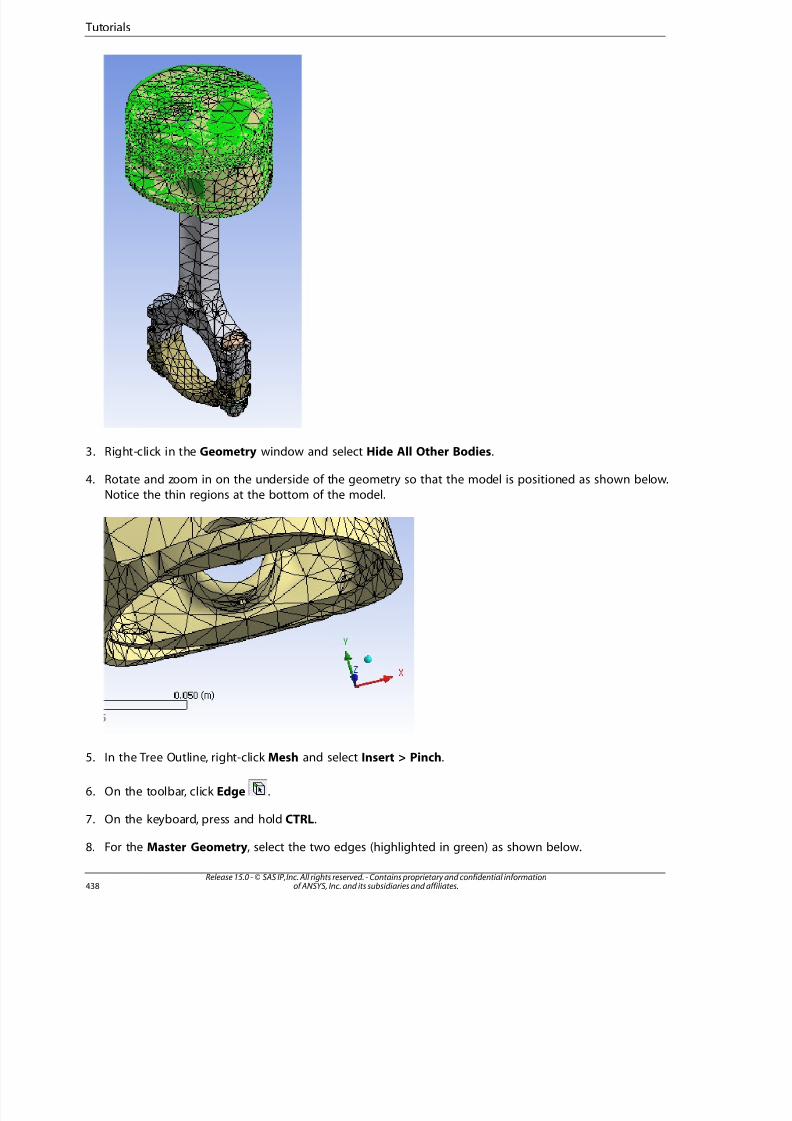
8/10/2019 ANSYS Meshing Users Guide
http://slidepdf.com/reader/full/ansys-meshing-users-guide 446/491
3. Right-click in the Geometry window and select Hide All Other Bodies.
4. Rotate and zoom in on the underside of the geometry so that the model is positioned as shown below.
Notice the thin regions at the bottom of the model.
5. In the Tree Outline, right-click Mesh and select Insert > Pinch.
6. On the toolbar, click Edge .
7. On the keyboard, press and hold CTRL.
8. For the Master Geometry, select the two edges (highlighted in green) as shown below.
Release 15.0 - © SAS IP, Inc. All rights reserved. - Contains proprietary and confidential informationof ANSYS, Inc. and its subsidiaries and affiliates.438
Tutorials
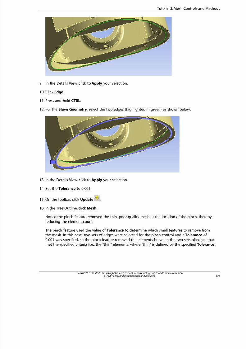
8/10/2019 ANSYS Meshing Users Guide
http://slidepdf.com/reader/full/ansys-meshing-users-guide 447/491
9. In the Details View, click to Apply your selection.
10. Click Edge.
11. Press and hold CTRL.
12. For the Slave Geometry, select the two edges (highlighted in green) as shown below.
13. In the Details View, click to Apply your selection.
14. Set the Tolerance to 0.001.
15. On the toolbar, click Update .
16. In the Tree Outline, click Mesh.
Notice the pinch feature removed the thin, poor quality mesh at the location of the pinch, thereby
reducing the element count.
The pinch feature used the value of Tolerance to determine which small features to remove fromthe mesh. In this case, two sets of edges were selected for the pinch control and a Tolerance of
0.001 was specified, so the pinch feature removed the elements between the two sets of edges thatmet the specified criteria (i.e., the “thin” elements, where "thin" is defined by the specified Tolerance).
439Release 15.0 - © SAS IP, Inc. All rights reserved. - Contains proprietary and confidential informationof ANSYS, Inc. and its subsidiaries and affiliates.
Tutorial 3: Mesh Controls and Methods

8/10/2019 ANSYS Meshing Users Guide
http://slidepdf.com/reader/full/ansys-meshing-users-guide 448/491
17. On the triad located in the lower right corner of the Geometry window, click the sphere to return the
view to isometric.
18. Right-click the Geometry window and select Show All Bodies.
Defining Mapped Face Meshing
This part of the tutorial demonstrates how to use mapped face meshing controls. Mapped face meshingcontrols attempt to generate a mapped mesh on selected faces. The Meshing application determines
a suitable number of divisions for the edges on the boundary face automatically. If you specify thenumber of divisions on the edge with a Sizing control, the Meshing application attempts to enforcethose divisions.
1. On the toolbar, click Body .
2. In the Geometry window, select the bottom of the piston as shown below.
Release 15.0 - © SAS IP, Inc. All rights reserved. - Contains proprietary and confidential informationof ANSYS, Inc. and its subsidiaries and affiliates.440
Tutorials
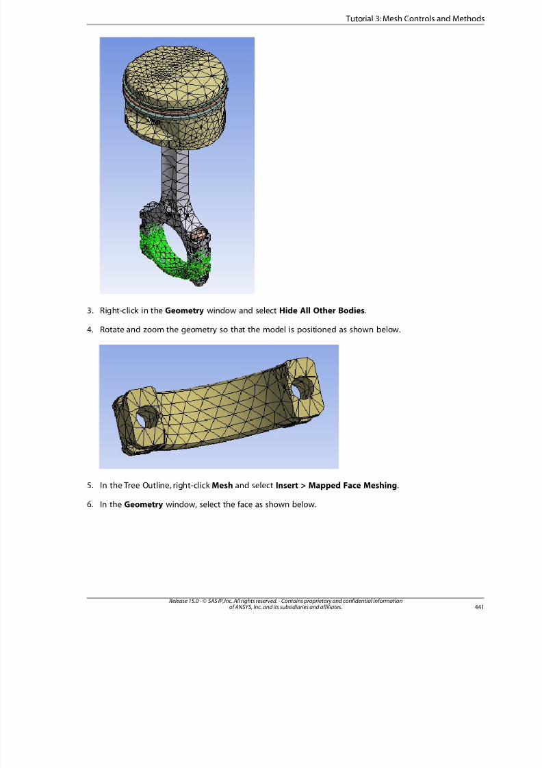
8/10/2019 ANSYS Meshing Users Guide
http://slidepdf.com/reader/full/ansys-meshing-users-guide 449/491
3. Right-click in the Geometry window and select Hide All Other Bodies.
4. Rotate and zoom the geometry so that the model is positioned as shown below.
5. In the Tree Outline, right-click Mesh and select Insert > Mapped Face Meshing.
6. In the Geometry window, select the face as shown below.
44Release 15.0 - © SAS IP, Inc. All rights reserved. - Contains proprietary and confidential informationof ANSYS, Inc. and its subsidiaries and affiliates.
Tutorial 3: Mesh Controls and Methods
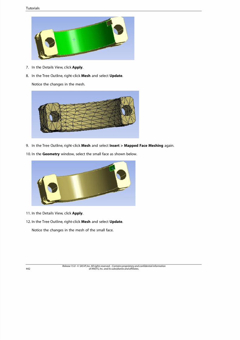
8/10/2019 ANSYS Meshing Users Guide
http://slidepdf.com/reader/full/ansys-meshing-users-guide 450/491
7. In the Details View, click Apply.
8. In the Tree Outline, right-click Mesh and select Update.
Notice the changes in the mesh.
9. In the Tree Outline, right-click Mesh and select Insert > Mapped Face Meshing again.
10. In the Geometry window, select the small face as shown below.
11. In the Details View, click Apply.
12. In the Tree Outline, right-click Mesh and select Update.
Notice the changes in the mesh of the small face.
Release 15.0 - © SAS IP, Inc. All rights reserved. - Contains proprietary and confidential informationof ANSYS, Inc. and its subsidiaries and affiliates.442
Tutorials

8/10/2019 ANSYS Meshing Users Guide
http://slidepdf.com/reader/full/ansys-meshing-users-guide 451/491
13. In the Geometry window, right-click and select Show All Bodies.
14. On the triad located in the lower right corner of the Geometry window, click the sphere to return theview to isometric.
Using the MultiZone Mesh Method
This part of the tutorial demonstrates how to obtain a MultiZone mesh for one of the bodies in thepiston.
1. In the Tree Outline, right-click Virtual Topology and select Delete All Virtual Entities.
2. Click Yes to delete the virtual entities.
3. On the toolbar, click Body .
4. In the Geometry window, select the bolt on the bottom left as shown below.
443Release 15.0 - © SAS IP, Inc. All rights reserved. - Contains proprietary and confidential informationof ANSYS, Inc. and its subsidiaries and affiliates.
Tutorial 3: Mesh Controls and Methods
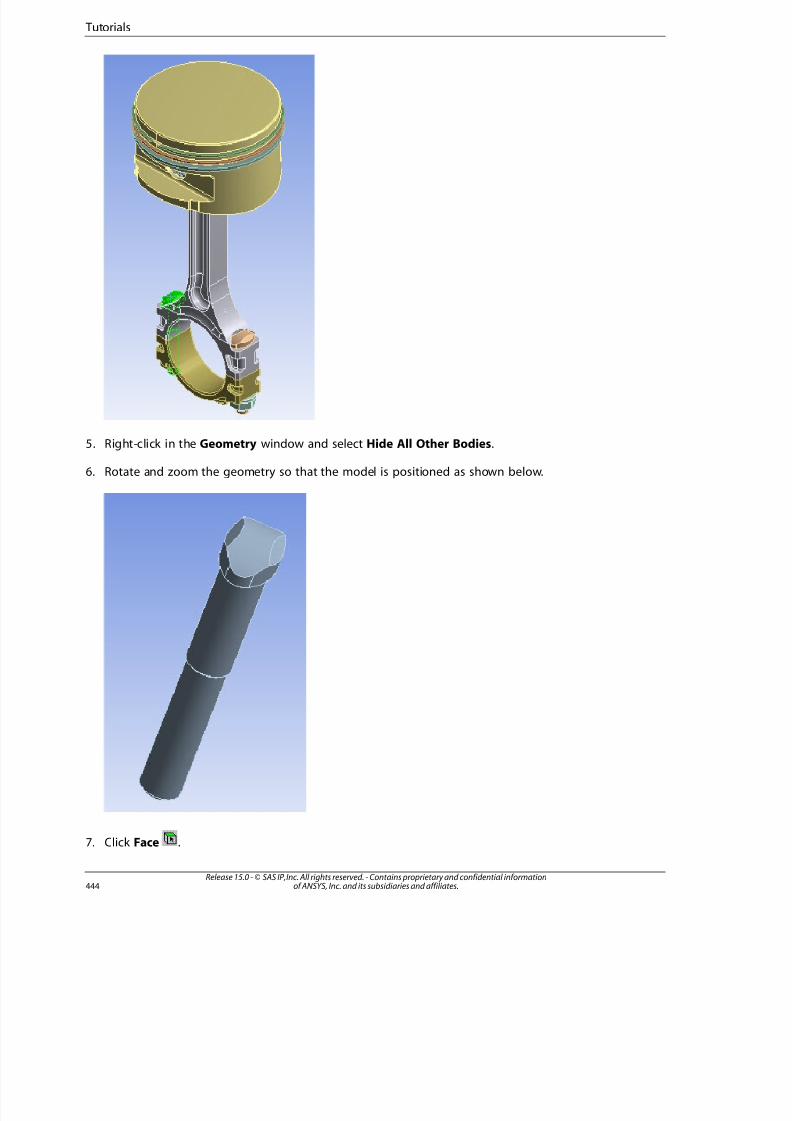
8/10/2019 ANSYS Meshing Users Guide
http://slidepdf.com/reader/full/ansys-meshing-users-guide 452/491
5. Right-click in the Geometry window and select Hide All Other Bodies.
6. Rotate and zoom the geometry so that the model is positioned as shown below.
7. Click Face .
Release 15.0 - © SAS IP, Inc. All rights reserved. - Contains proprietary and confidential informationof ANSYS, Inc. and its subsidiaries and affiliates.444
Tutorials
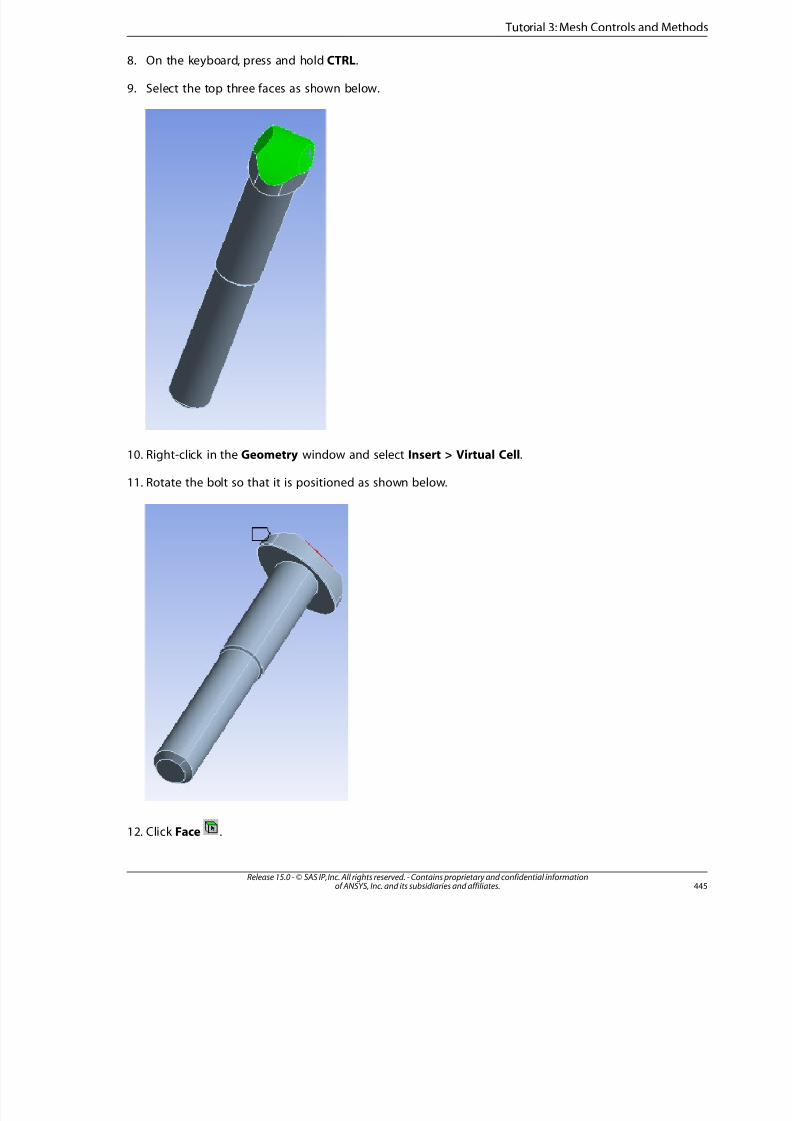
8/10/2019 ANSYS Meshing Users Guide
http://slidepdf.com/reader/full/ansys-meshing-users-guide 453/491
8. On the keyboard, press and hold CTRL.
9. Select the top three faces as shown below.
10. Right-click in the Geometry window and select Insert > Virtual Cell.
11. Rotate the bolt so that it is positioned as shown below.
12. Click Face .
445Release 15.0 - © SAS IP, Inc. All rights reserved. - Contains proprietary and confidential informationof ANSYS, Inc. and its subsidiaries and affiliates.
Tutorial 3: Mesh Controls and Methods
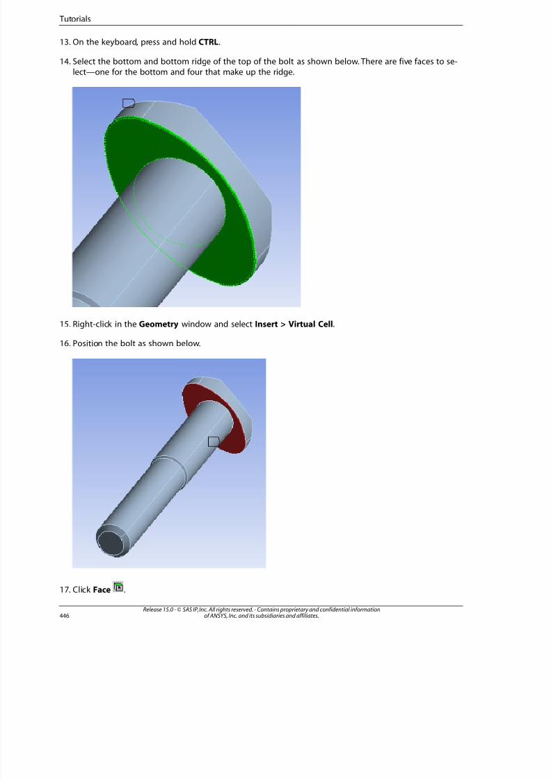
8/10/2019 ANSYS Meshing Users Guide
http://slidepdf.com/reader/full/ansys-meshing-users-guide 454/491
13. On the keyboard, press and hold CTRL.
14. Select the bottom and bottom ridge of the top of the bolt as shown below. There are five faces to se-lect—one for the bottom and four that make up the ridge.
15. Right-click in the Geometry window and select Insert > Virtual Cell.
16. Position the bolt as shown below.
17. Click Face .
Release 15.0 - © SAS IP, Inc. All rights reserved. - Contains proprietary and confidential informationof ANSYS, Inc. and its subsidiaries and affiliates.446
Tutorials

8/10/2019 ANSYS Meshing Users Guide
http://slidepdf.com/reader/full/ansys-meshing-users-guide 455/491
18. On the keyboard, press and hold CTRL.
19. Select the bottom three faces of the bolt as shown below.
20. Right-click in the Geometry window and select Insert > Virtual Cell.
21. In the Tree Outline, right-click Mesh and select Insert > Method.
22. In the Geometry window, select the bolt.
23. In the Details View, click Apply.
24. In the Details View, change Method to MultiZone.
25. Change Src/Trg Selection to Manual Source.
There are three source faces to select.
26. Click Face .
27. On the keyboard, press and hold CTRL.
28. Select the first two faces as shown below.
447Release 15.0 - © SAS IP, Inc. All rights reserved. - Contains proprietary and confidential informationof ANSYS, Inc. and its subsidiaries and affiliates.
Tutorial 3: Mesh Controls and Methods
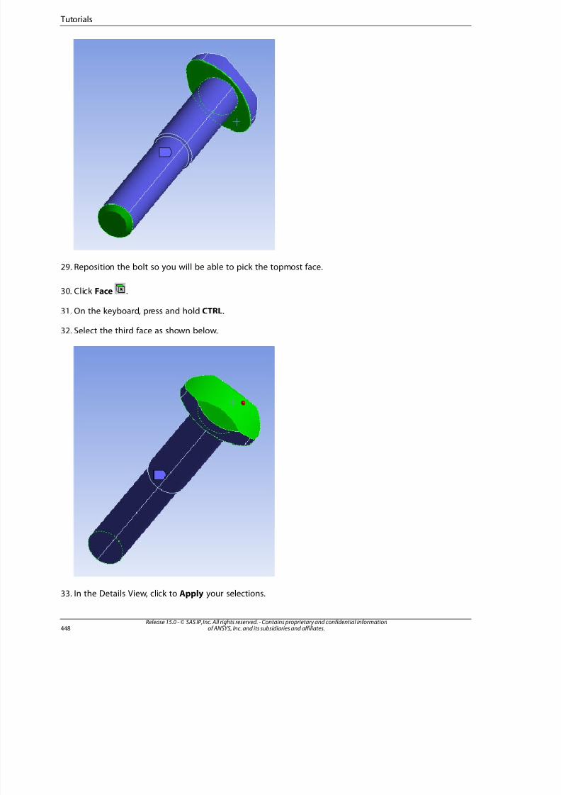
8/10/2019 ANSYS Meshing Users Guide
http://slidepdf.com/reader/full/ansys-meshing-users-guide 456/491
29. Reposition the bolt so you will be able to pick the topmost face.
30. Click Face .
31. On the keyboard, press and hold CTRL.
32. Select the third face as shown below.
33. In the Details View, click to Apply your selections.
Release 15.0 - © SAS IP, Inc. All rights reserved. - Contains proprietary and confidential informationof ANSYS, Inc. and its subsidiaries and affiliates.448
Tutorials
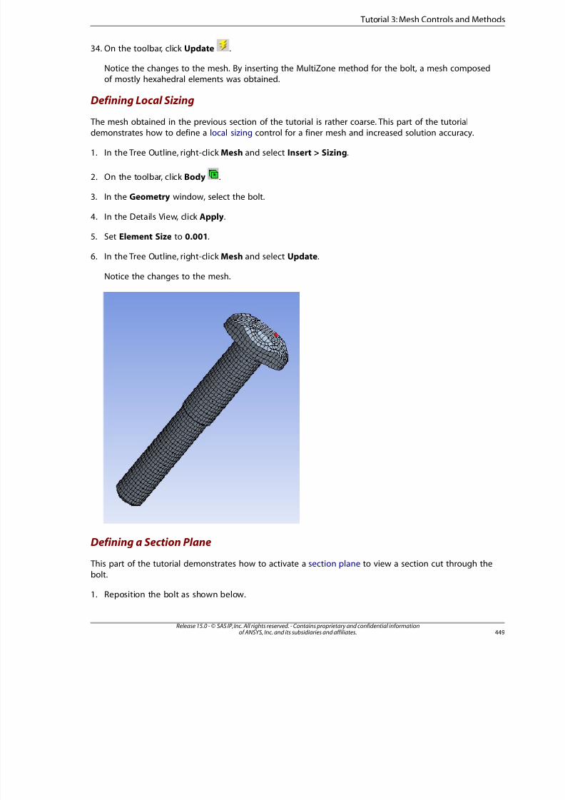
8/10/2019 ANSYS Meshing Users Guide
http://slidepdf.com/reader/full/ansys-meshing-users-guide 457/491
34. On the toolbar, click Update .
Notice the changes to the mesh. By inserting the MultiZone method for the bolt, a mesh composedof mostly hexahedral elements was obtained.
Defining Local Sizing
The mesh obtained in the previous section of the tutorial is rather coarse. This part of the tutorialdemonstrates how to define a local sizing control for a finer mesh and increased solution accuracy.
1. In the Tree Outline, right-click Mesh and select Insert > Sizing.
2. On the toolbar, click Body .
3. In the Geometry window, select the bolt.
4. In the Details View, click Apply.
5. Set Element Size to 0.001.
6. In the Tree Outline, right-click Mesh and select Update.
Notice the changes to the mesh.
Defining a Section Plane
This part of the tutorial demonstrates how to activate a section plane to view a section cut through the
bolt.
1. Reposition the bolt as shown below.
449Release 15.0 - © SAS IP, Inc. All rights reserved. - Contains proprietary and confidential informationof ANSYS, Inc. and its subsidiaries and affiliates.
Tutorial 3: Mesh Controls and Methods
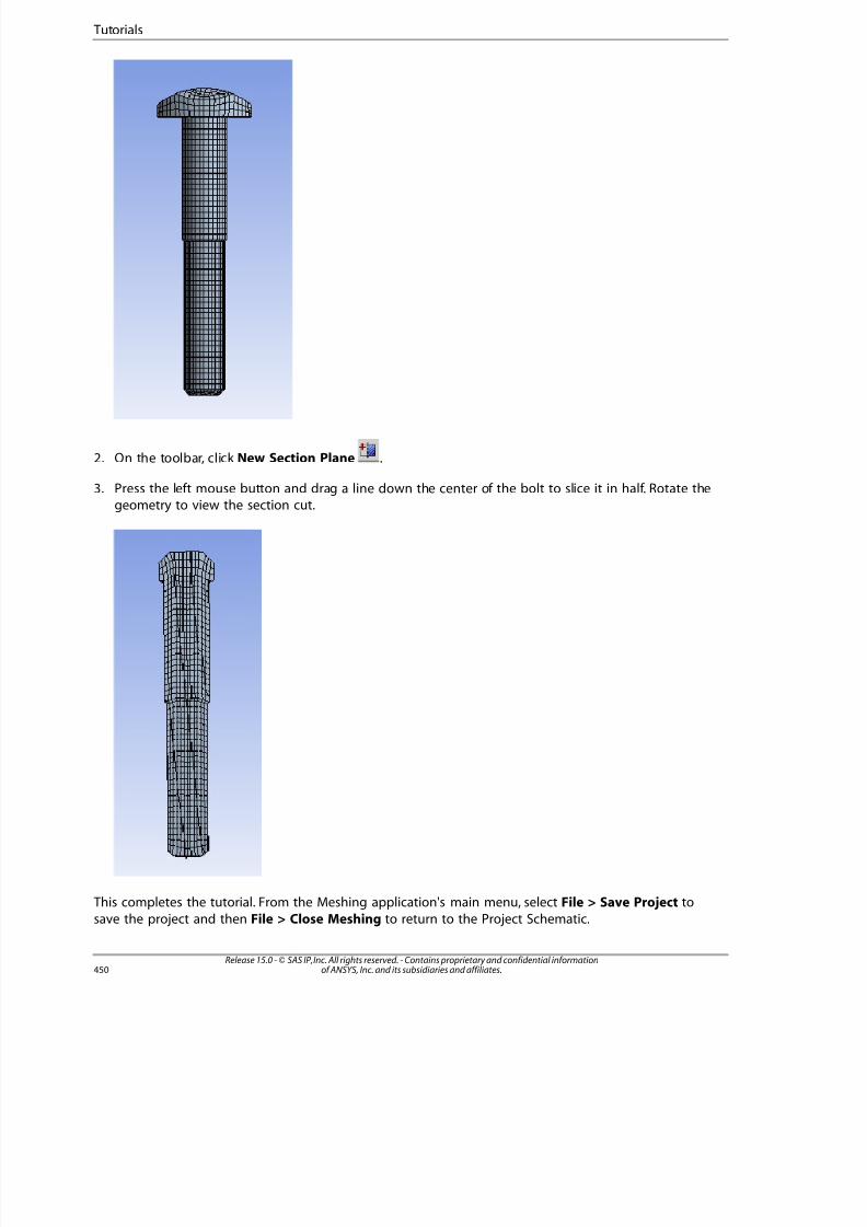
8/10/2019 ANSYS Meshing Users Guide
http://slidepdf.com/reader/full/ansys-meshing-users-guide 458/491
2. On the toolbar, click New Section Plane .
3. Press the left mouse button and drag a line down the center of the bolt to slice it in half. Rotate thegeometry to view the section cut.
This completes the tutorial. From the Meshing application's main menu, select File > Save Project to
save the project and then File > Close Meshing to return to the Project Schematic.
Release 15.0 - © SAS IP, Inc. All rights reserved. - Contains proprietary and confidential informationof ANSYS, Inc. and its subsidiaries and affiliates.450
Tutorials
8/10/2019 ANSYS Meshing Users Guide
http://slidepdf.com/reader/full/ansys-meshing-users-guide 459/491
You can exit ANSYS Workbench by selecting File > Exit from the main menu.
Tutorial 4: Advanced Size Function
This tutorial illustrates the use of the Meshing application's advanced size function feature. This featureallows for greater control over global sizing options, including the following properties:
• Angles between normals for adjacent mesh elements (Curvature-type size function)
• Number of mesh elements employed in the gaps between two geometric entities (Proximity-type sizefunction)
• Gradation between minimum and maximum sizes based on a specified growth rate (All size functions)
During the tutorial, the influence of each of the following advanced size function options on a meshwill be demonstrated:
• None (Off )
• Fixed
• Proximity
• Curvature
• Proximity and Curvature
This tutorial requires you to have a copy of the ANSYS Workbench project file nacelle.wbpj and
the project folder nacelle_files and its contents.
To access tutorials and their input files on the ANSYS Customer Portal, go to http://support.ansys.com/training.
To prepare for running this tutorial:
1. Set up a working folder on the computer you will be using.
2. Download the tutorial input file (Nacelle.zip) for this tutorial.
3. Unzip Nacelle.zip to your working folder.
You can proceed to Tutorial Setup (p. 451).
Tutorial Setup
Opening the Project
1. Open ANSYS Workbench.
2. Select File > Open... from the main menu.
3. In the file browser that opens, locate and open the file nacelle.wbpj.
Now that the tutorial is set up, you can proceed to Mesh Generation (p. 452).
45Release 15.0 - © SAS IP, Inc. All rights reserved. - Contains proprietary and confidential informationof ANSYS, Inc. and its subsidiaries and affiliates.
Tutorial 4: Advanced Size Function
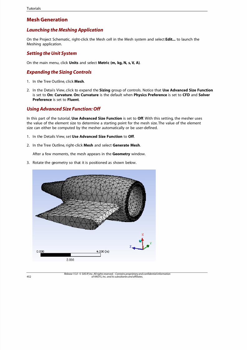
8/10/2019 ANSYS Meshing Users Guide
http://slidepdf.com/reader/full/ansys-meshing-users-guide 460/491
Mesh Generation
Launching the Meshing Application
On the Project Schematic, right-click the Mesh cell in the Mesh system and select Edit... to launch theMeshing application.
Setting the Unit SystemOn the main menu, click Units and select Metric (m, kg, N, s, V, A).
Expanding the Sizing Controls
1. In the Tree Outline, click Mesh.
2. In the Details View, click to expand the Sizing group of controls. Notice that Use Advanced Size Functionis set to On: Curvature. On: Curvature is the default when Physics Preference is set to CFD and SolverPreference is set to Fluent.
Using Advanced Size Function: Off
In this part of the tutorial, Use Advanced Size Function is set to Off . With this setting, the mesher usesthe value of the element size to determine a starting point for the mesh size. The value of the elementsize can either be computed by the mesher automatically or be user-defined.
1. In the Details View, set Use Advanced Size Function to Off .
2. In the Tree Outline, right-click Mesh and select Generate Mesh.
After a few moments, the mesh appears in the Geometry window.
3. Rotate the geometry so that it is positioned as shown below.
Release 15.0 - © SAS IP, Inc. All rights reserved. - Contains proprietary and confidential informationof ANSYS, Inc. and its subsidiaries and affiliates.452
Tutorials
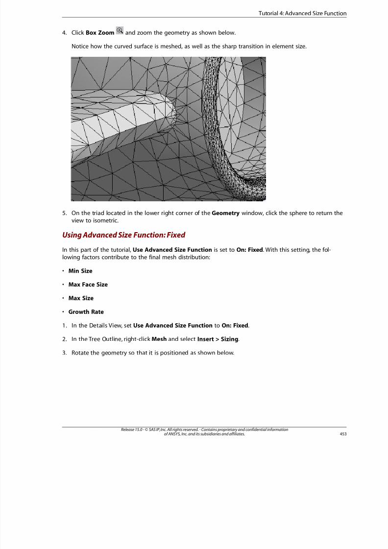
8/10/2019 ANSYS Meshing Users Guide
http://slidepdf.com/reader/full/ansys-meshing-users-guide 461/491
4. Click Box Zoom and zoom the geometry as shown below.
Notice how the curved surface is meshed, as well as the sharp transition in element size.
5. On the triad located in the lower right corner of the Geometry window, click the sphere to return theview to isometric.
Using Advanced Size Function: Fixed
In this part of the tutorial, Use Advanced Size Function is set to On: Fixed. With this setting, the fol-
lowing factors contribute to the final mesh distribution:
• Min Size
• Max Face Size
• Max Size
• Growth Rate
1. In the Details View, set Use Advanced Size Function to On: Fixed.
2. In the Tree Outline, right-click Mesh and select Insert > Sizing.
3. Rotate the geometry so that it is positioned as shown below.
453Release 15.0 - © SAS IP, Inc. All rights reserved. - Contains proprietary and confidential informationof ANSYS, Inc. and its subsidiaries and affiliates.
Tutorial 4: Advanced Size Function
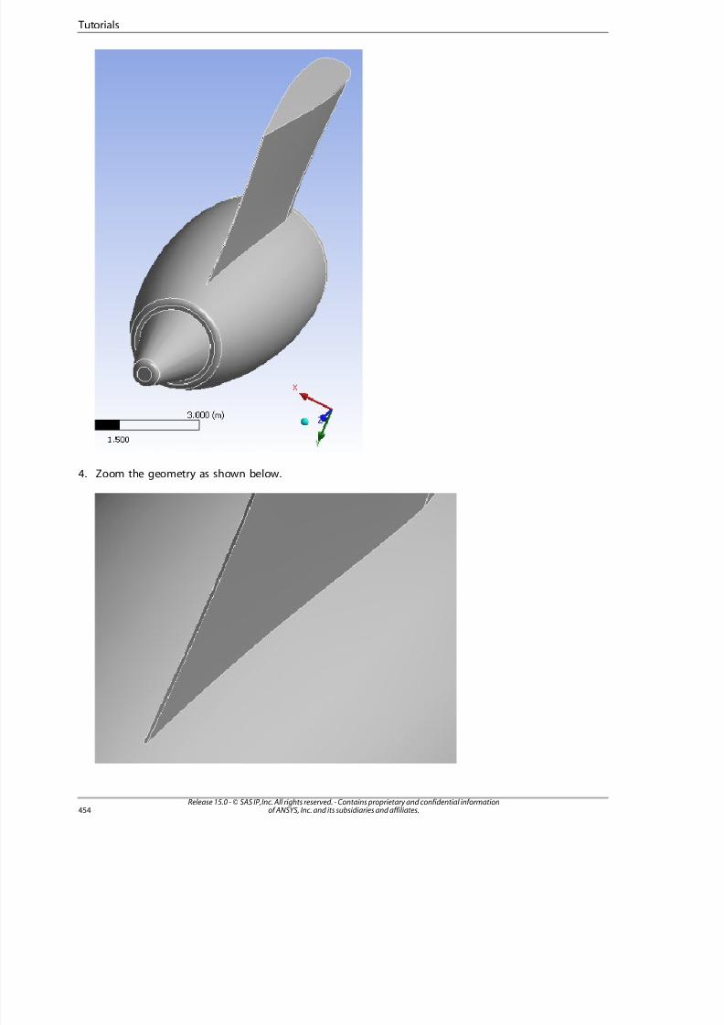
8/10/2019 ANSYS Meshing Users Guide
http://slidepdf.com/reader/full/ansys-meshing-users-guide 462/491
4. Zoom the geometry as shown below.
Release 15.0 - © SAS IP, Inc. All rights reserved. - Contains proprietary and confidential informationof ANSYS, Inc. and its subsidiaries and affiliates.454
Tutorials
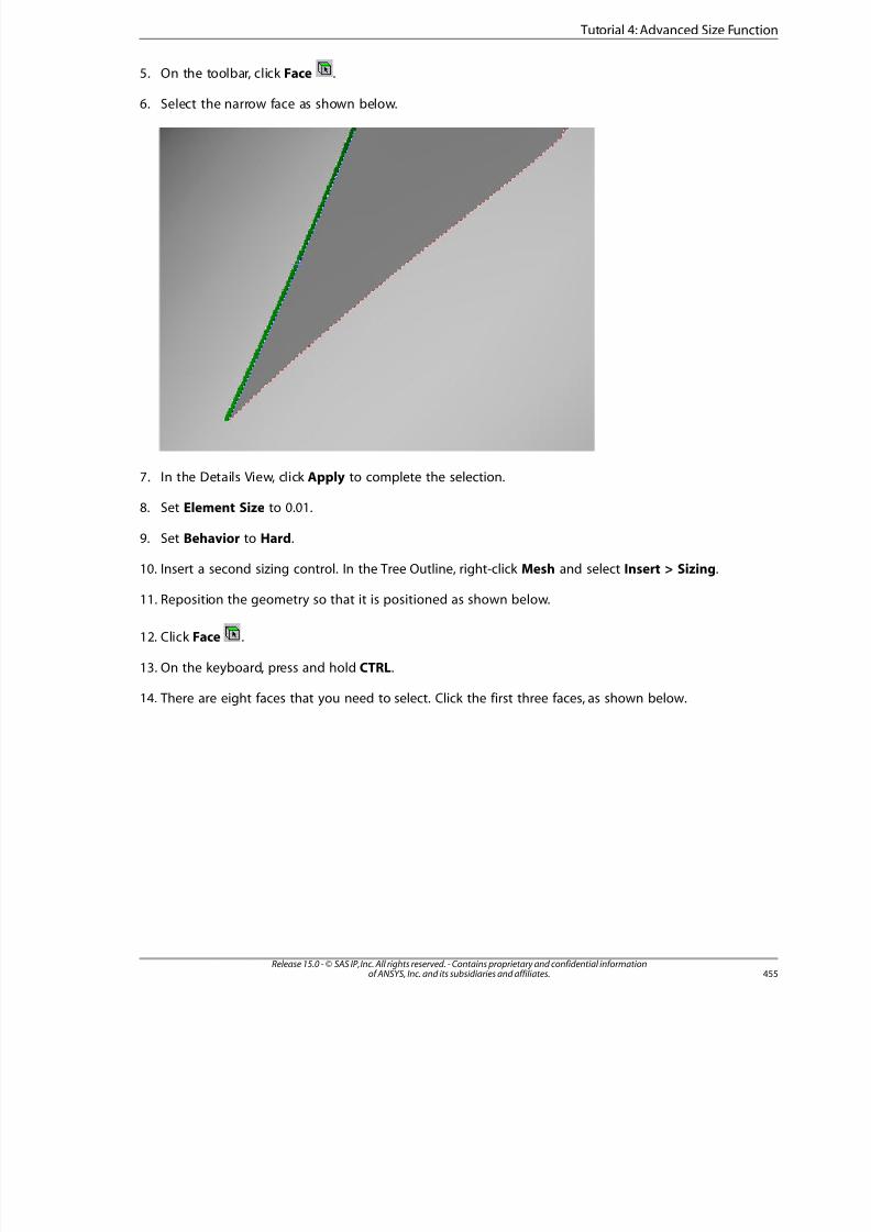
8/10/2019 ANSYS Meshing Users Guide
http://slidepdf.com/reader/full/ansys-meshing-users-guide 463/491
5. On the toolbar, click Face .
6. Select the narrow face as shown below.
7. In the Details View, click Apply to complete the selection.
8. Set Element Size to 0.01.
9. Set Behavior to Hard.
10. Insert a second sizing control. In the Tree Outline, right-click Mesh and select Insert > Sizing.
11. Reposition the geometry so that it is positioned as shown below.
12. Click Face .
13. On the keyboard, press and hold CTRL.
14. There are eight faces that you need to select. Click the first three faces, as shown below.
455Release 15.0 - © SAS IP, Inc. All rights reserved. - Contains proprietary and confidential informationof ANSYS, Inc. and its subsidiaries and affiliates.
Tutorial 4: Advanced Size Function
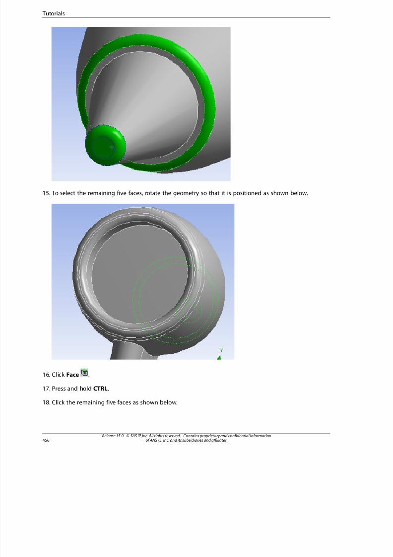
8/10/2019 ANSYS Meshing Users Guide
http://slidepdf.com/reader/full/ansys-meshing-users-guide 464/491
15. To select the remaining five faces, rotate the geometry so that it is positioned as shown below.
16. Click Face .
17. Press and hold CTRL.
18. Click the remaining five faces as shown below.
Release 15.0 - © SAS IP, Inc. All rights reserved. - Contains proprietary and confidential informationof ANSYS, Inc. and its subsidiaries and affiliates.456
Tutorials
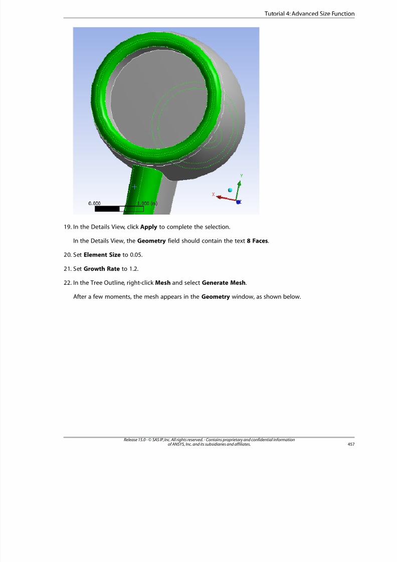
8/10/2019 ANSYS Meshing Users Guide
http://slidepdf.com/reader/full/ansys-meshing-users-guide 465/491
19. In the Details View, click Apply to complete the selection.
In the Details View, the Geometry field should contain the text 8 Faces.
20. Set Element Size to 0.05.
21. Set Growth Rate to 1.2.
22. In the Tree Outline, right-click Mesh and select Generate Mesh.
After a few moments, the mesh appears in the Geometry window, as shown below.
457Release 15.0 - © SAS IP, Inc. All rights reserved. - Contains proprietary and confidential informationof ANSYS, Inc. and its subsidiaries and affiliates.
Tutorial 4: Advanced Size Function
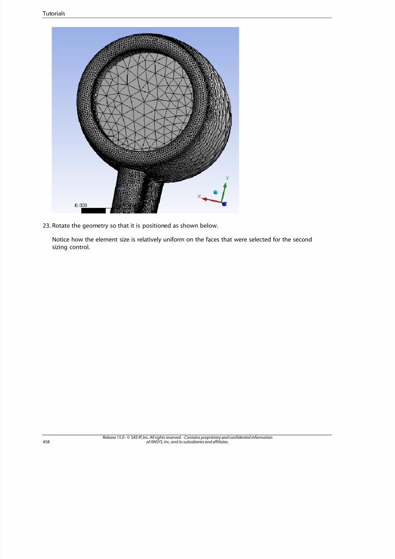
8/10/2019 ANSYS Meshing Users Guide
http://slidepdf.com/reader/full/ansys-meshing-users-guide 466/491
23. Rotate the geometry so that it is positioned as shown below.
Notice how the element size is relatively uniform on the faces that were selected for the secondsizing control.
Release 15.0 - © SAS IP, Inc. All rights reserved. - Contains proprietary and confidential informationof ANSYS, Inc. and its subsidiaries and affiliates.458
Tutorials
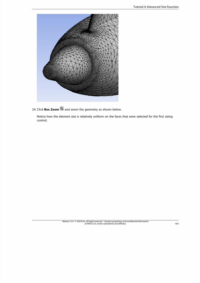
8/10/2019 ANSYS Meshing Users Guide
http://slidepdf.com/reader/full/ansys-meshing-users-guide 467/491
24. Click Box Zoom and zoom the geometry as shown below.
Notice how the element size is relatively uniform on the faces that were selected for the first sizing
control.
459Release 15.0 - © SAS IP, Inc. All rights reserved. - Contains proprietary and confidential informationof ANSYS, Inc. and its subsidiaries and affiliates.
Tutorial 4: Advanced Size Function
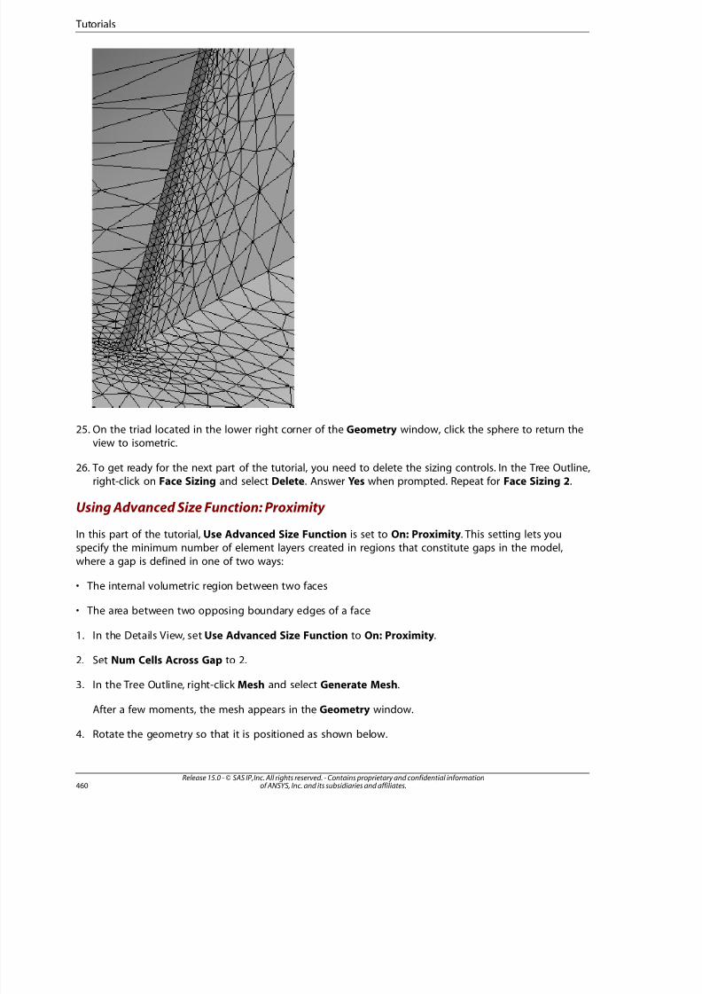
8/10/2019 ANSYS Meshing Users Guide
http://slidepdf.com/reader/full/ansys-meshing-users-guide 468/491
25. On the triad located in the lower right corner of the Geometry window, click the sphere to return theview to isometric.
26. To get ready for the next part of the tutorial, you need to delete the sizing controls. In the Tree Outline,right-click on Face Sizing and select Delete. Answer Yes when prompted. Repeat for Face Sizing 2.
Using Advanced Size Function: Proximity
In this part of the tutorial, Use Advanced Size Function is set to On: Proximity. This setting lets youspecify the minimum number of element layers created in regions that constitute gaps in the model,
where a gap is defined in one of two ways:
• The internal volumetric region between two faces
• The area between two opposing boundary edges of a face
1. In the Details View, set Use Advanced Size Function to On: Proximity.
2. Set Num Cells Across Gap to 2.
3. In the Tree Outline, right-click Mesh and select Generate Mesh.
After a few moments, the mesh appears in the Geometry window.
4. Rotate the geometry so that it is positioned as shown below.
Release 15.0 - © SAS IP, Inc. All rights reserved. - Contains proprietary and confidential informationof ANSYS, Inc. and its subsidiaries and affiliates.460
Tutorials
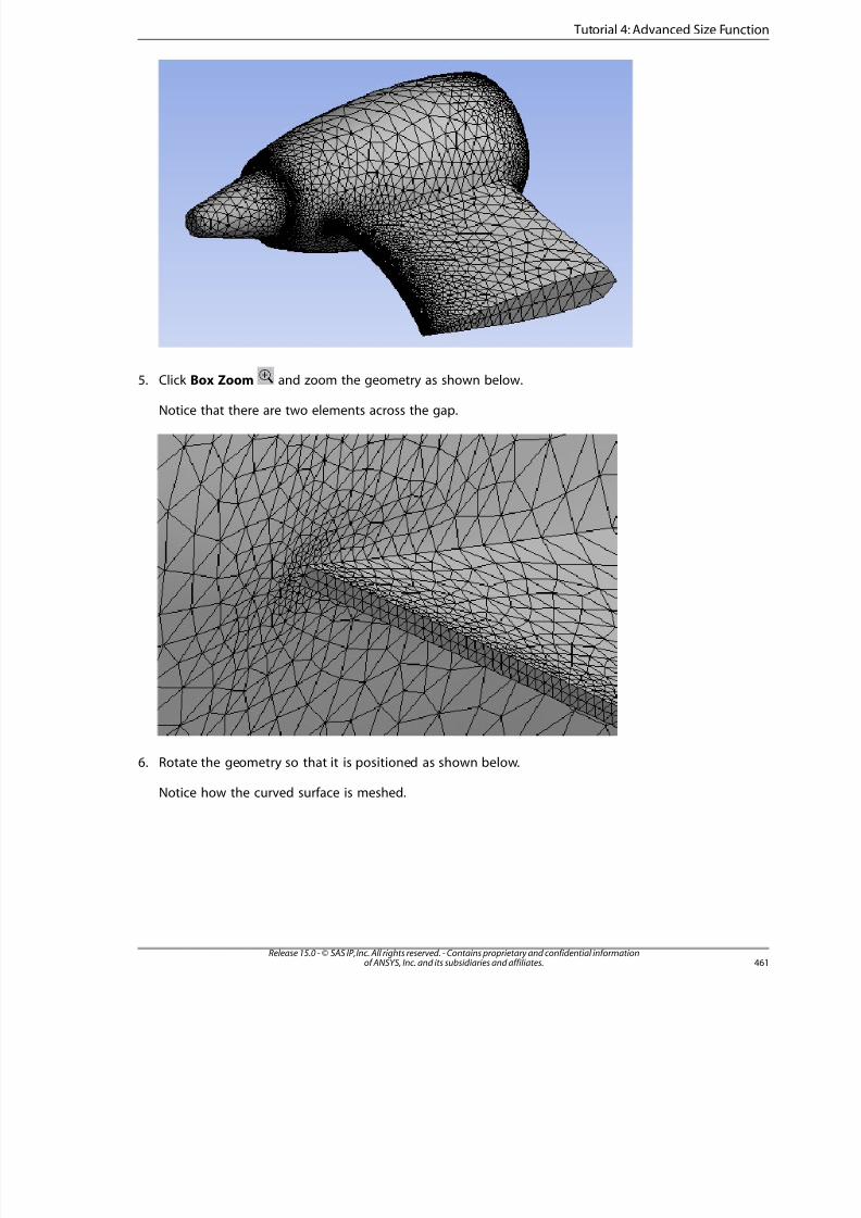
8/10/2019 ANSYS Meshing Users Guide
http://slidepdf.com/reader/full/ansys-meshing-users-guide 469/491
5. Click Box Zoom and zoom the geometry as shown below.
Notice that there are two elements across the gap.
6. Rotate the geometry so that it is positioned as shown below.
Notice how the curved surface is meshed.
46Release 15.0 - © SAS IP, Inc. All rights reserved. - Contains proprietary and confidential informationof ANSYS, Inc. and its subsidiaries and affiliates.
Tutorial 4: Advanced Size Function
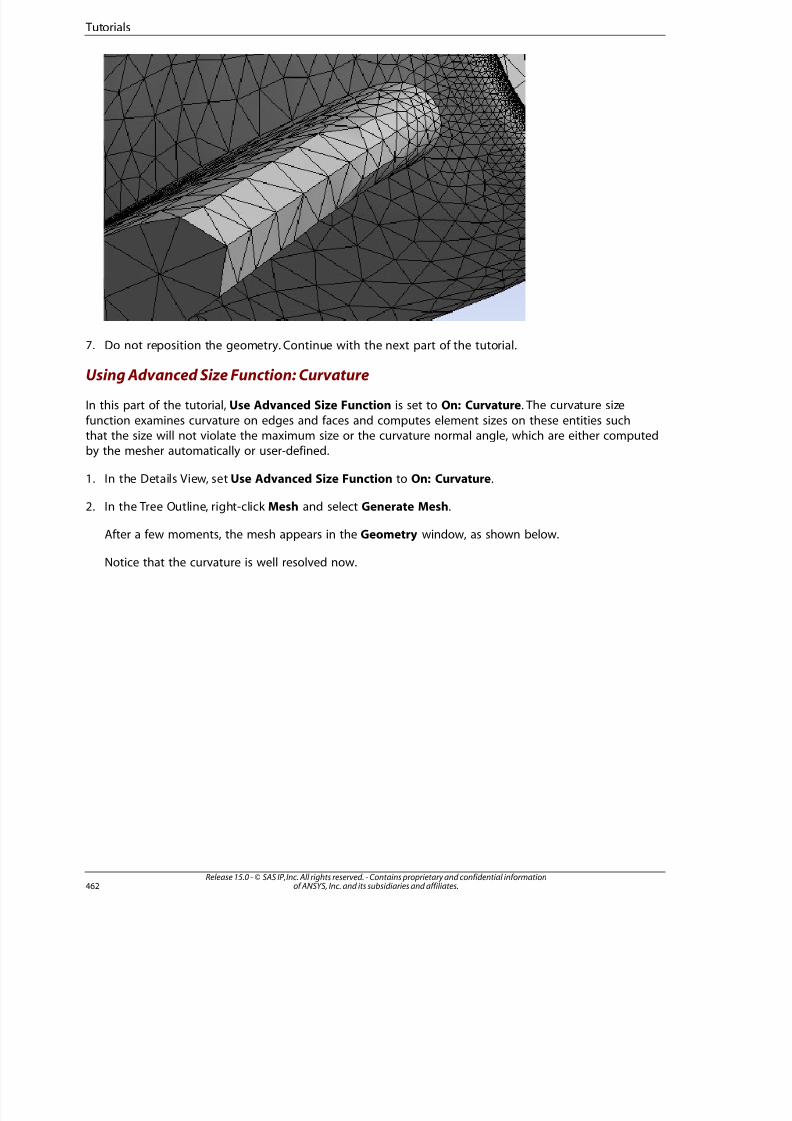
8/10/2019 ANSYS Meshing Users Guide
http://slidepdf.com/reader/full/ansys-meshing-users-guide 470/491
7. Do not reposition the geometry. Continue with the next part of the tutorial.
Using Advanced Size Function: Curvature
In this part of the tutorial, Use Advanced Size Function is set to On: Curvature. The curvature size
function examines curvature on edges and faces and computes element sizes on these entities suchthat the size will not violate the maximum size or the curvature normal angle, which are either computedby the mesher automatically or user-defined.
1. In the Details View, set Use Advanced Size Function to On: Curvature.
2. In the Tree Outline, right-click Mesh and select Generate Mesh.
After a few moments, the mesh appears in the Geometry window, as shown below.
Notice that the curvature is well resolved now.
Release 15.0 - © SAS IP, Inc. All rights reserved. - Contains proprietary and confidential informationof ANSYS, Inc. and its subsidiaries and affiliates.462
Tutorials
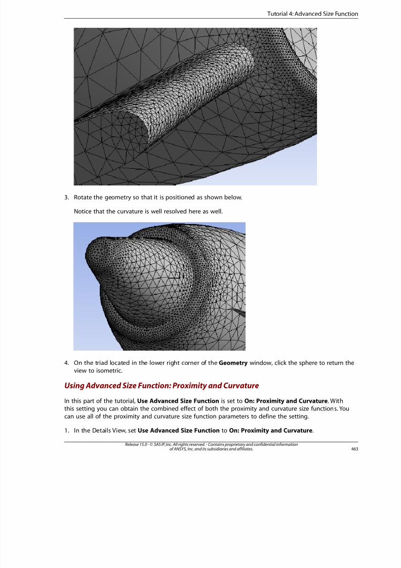
8/10/2019 ANSYS Meshing Users Guide
http://slidepdf.com/reader/full/ansys-meshing-users-guide 471/491
3. Rotate the geometry so that it is positioned as shown below.
Notice that the curvature is well resolved here as well.
4. On the triad located in the lower right corner of the Geometry window, click the sphere to return the
view to isometric.
Using Advanced Size Function: Proximity and Curvature
In this part of the tutorial, Use Advanced Size Function is set to On: Proximity and Curvature. Withthis setting you can obtain the combined effect of both the proximity and curvature size functions. You
can use all of the proximity and curvature size function parameters to define the setting.
1. In the Details View, set Use Advanced Size Function to On: Proximity and Curvature.
463Release 15.0 - © SAS IP, Inc. All rights reserved. - Contains proprietary and confidential informationof ANSYS, Inc. and its subsidiaries and affiliates.
Tutorial 4: Advanced Size Function
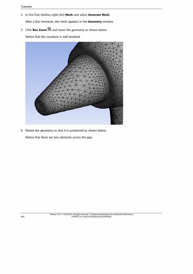
8/10/2019 ANSYS Meshing Users Guide
http://slidepdf.com/reader/full/ansys-meshing-users-guide 472/491
2. In the Tree Outline, right-click Mesh and select Generate Mesh.
After a few moments, the mesh appears in the Geometry window.
3. Click Box Zoom and zoom the geometry as shown below.
Notice that the curvature is well resolved.
4. Rotate the geometry so that it is positioned as shown below.
Notice that there are two elements across the gap.
Release 15.0 - © SAS IP, Inc. All rights reserved. - Contains proprietary and confidential informationof ANSYS, Inc. and its subsidiaries and affiliates.464
Tutorials
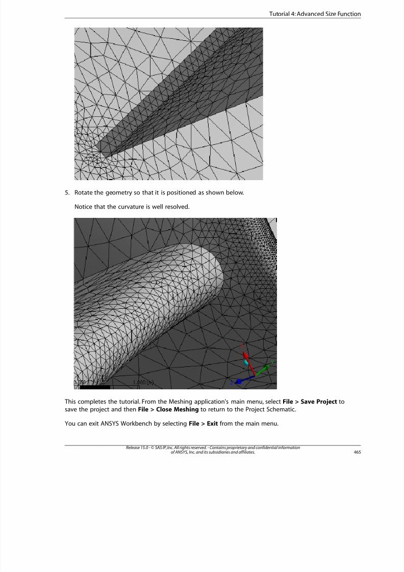
8/10/2019 ANSYS Meshing Users Guide
http://slidepdf.com/reader/full/ansys-meshing-users-guide 473/491
5. Rotate the geometry so that it is positioned as shown below.
Notice that the curvature is well resolved.
This completes the tutorial. From the Meshing application's main menu, select File > Save Project tosave the project and then File > Close Meshing to return to the Project Schematic.
You can exit ANSYS Workbench by selecting File > Exit from the main menu.
465Release 15.0 - © SAS IP, Inc. All rights reserved. - Contains proprietary and confidential informationof ANSYS, Inc. and its subsidiaries and affiliates.
Tutorial 4: Advanced Size Function

8/10/2019 ANSYS Meshing Users Guide
http://slidepdf.com/reader/full/ansys-meshing-users-guide 474/491
Tutorial 5: Thin Sweep Meshing of a Multibody Part
The Meshing application supports thin sweep meshing for both single body and multibody parts. Forsingle body parts, multiple elements through the thickness can be defined. For multibody parts, onlyone division through the thickness of the thin sweep is possible. A benefit of multibody part meshing
is its creation of conformal mesh between bodies. This tutorial illustrates the use of the Meshing applic-ation's thin sweep meshing feature to mesh a truck frame modeled as a multibody part. Topics covered
in this tutorial include:
• Inserting a Sweep mesh method for a part and for a single body
• Setting Automatic Thin and Manual Thin options for the Src/Trg Selection control
• Troubleshooting meshing failure and use of selective meshing to mesh individual bodies
• Suppressing and unsuppressing bodies in a multibody part and its effects on the mesh
• Manually selecting source faces for the sweep and using the Extend to Limits menu option to select alltangent faces
This tutorial requires you to have a copy of the geometry file TRUCK_FRAME_MODEL_NAMES.agdb.
To access tutorials and their input files on the ANSYS Customer Portal, go to http://support.ansys.com/
training.
To prepare for running this tutorial:
1. Set up a working folder on the computer you will be using.
2. Download the tutorial input file (Truck_Frame_Model_Names.zip) for this tutorial.
3. Unzip Truck_Frame_Model_Names.zip to your working folder.
You can proceed to Tutorial Setup (p. 466).
Tutorial Setup
Creating the Project
1. Open ANSYS Workbench.
2. Double-click on the Static Structural analysis system in the Toolbox to add a Static Structural system tothe Project Schematic.
3. Select File > Save from the main menu and save the project as THIN_SWEEP_MBPART.wbpj.
Importing the Geometry
1. Now add geometry to the project. On the Project Schematic, right-click the Geometry cell in the Static
Structural system and select Import Geometry > Browse....
2. In the file browser that opens, locate and open the file TRUCK_FRAME_MODEL_NAMES.agdb.
Release 15.0 - © SAS IP, Inc. All rights reserved. - Contains proprietary and confidential informationof ANSYS, Inc. and its subsidiaries and affiliates.466
Tutorials
8/10/2019 ANSYS Meshing Users Guide
http://slidepdf.com/reader/full/ansys-meshing-users-guide 475/491
The geometry is complete and does not require modifications. Notice the Geometry cell has an up-to-
date state .
Now that the tutorial is set up, you can proceed to Mesh Generation (p. 467).
Mesh Generation
Launching the Mechanical ApplicationOn the Project Schematic, right-click the Model cell in the Static Structural system and select Edit... tolaunch the Mechanical application.
Note
In this tutorial, Meshing application capabilities that are also available within the Mechanical
application are used.
Setting the Unit System
On the main menu, click Units and select Metric (mm, kg, N, s, mV, mA).
Expanding the Tree Outline
1. In the Tree Outline, click to expand the Geometry and Part (i.e., RAIL_ASSEM) objects.
2. Notice that the model consists of one multibody part that is made up of seven solid bodies.
Using the Automatic Thin Option
In this part of the tutorial, the Automatic Thin option for source/target selection will be used on the
part.
1. In the Tree Outline, right-click Mesh and select Insert > Method.
2. Right-click in the Geometry window and select Select All from the context menu.
3. In the Details View, click the Geometry field to apply your selection.
The value in the Geometry field confirms that all seven bodies are selected.
4. For Method, select Sweep.
5. For Src/Trg Selection, select Automatic Thin.
For multibody parts, remember that only one division through the thickness is possible. Notice thatSweep Num Divs is set to 1 by default, and cannot be changed.
6. In the Tree Outline, click the Mesh object.
7. In the Details View, click to expand the Sizing group of controls.
8. Set Element Size to 1.
9. In the Details View, click to expand the Advanced group of controls.
467Release 15.0 - © SAS IP, Inc. All rights reserved. - Contains proprietary and confidential informationof ANSYS, Inc. and its subsidiaries and affiliates.
Tutorial 5:Thin Sweep Meshing of a Multibody Part

8/10/2019 ANSYS Meshing Users Guide
http://slidepdf.com/reader/full/ansys-meshing-users-guide 476/491
10. Set Number of Retries to 0.
Not all bodies will be able to be meshed with the Automatic Thin option. When Number of Retriesis set to 0, the mesher does not try to re-mesh using smaller sizes. This means that it will fail tomesh sooner, thus allowing you to respond sooner by adding the necessary controls on the difficult(failed) bodies.
11. In the Tree Outline, right-click the Mesh object and select Generate Mesh.
After a short wait, the mesh generation fails.
Notice the small status icons to the left of the part/body listing in the Tree Outline. In a multibody
part all bodies are meshed at the same time to ensure a conformal mesh. When a multibody part
is meshed, the status icon to the left of the Part object changes from to to indicate the meshgeneration was successful. If one body fails, the entire mesh fails. Notice that the mesh is nowcolored maroon. Notice also that the status icon for the Part object (as well as for all seven bodies)
is still .
12. Examine the list of messages in the Messages window. To view the full text of a message you can eitherdouble-click on it, or right-click on it and select Show Message from the context menu.
In some cases, an error message may not provide enough information to identify the problem. Thisis why it is important to examine all of the messages, especially any warning messages, which maygive an indication of a subsequent related error.
In the case of this tutorial, the following warning message suggests an alternative course of action,which you will follow later in the tutorial:
Source Faces: For Thin Model Sweeping, the area of source faces should be
similar to that of the target faces. It has been detected that they are quite differ-ent. Please verify the source faces (highlighted faces) and try again. If the programgenerated source faces are not what you want, manually specify the source
faces.
To view the highlighted faces that are mentioned in the message, right-click on the message in themessage list and select Show Problematic Geometry from the context menu. Notice the faces thatare highlighted in green in the Geometry window, as shown below.
Release 15.0 - © SAS IP, Inc. All rights reserved. - Contains proprietary and confidential informationof ANSYS, Inc. and its subsidiaries and affiliates.468
Tutorials

8/10/2019 ANSYS Meshing Users Guide
http://slidepdf.com/reader/full/ansys-meshing-users-guide 477/491
You can visualize the bodies that are attached to these faces and thus failing to mesh by right-clicking in the Geometry window and selecting Go To > Corresponding Bodies in Tree.
Using the Manual Thin Option
In this part of the tutorial, the Manual Thin option for source/target selection will be used on two
bodies (i.e., the FRONT_RAIL and REAR_RAIL listed in the Tree Outline). This option requires you tomanually specify the source faces for these bodies.
In the Tree Outline, there should be three bodies selected:
1. FRONT_RAIL: We will be defining a manual thin sweep mesh method control on this body.
2. REAR_RAIL: We will be defining a manual thin sweep mesh method control on this body.
3. RAIL: This body is selected because it shares faces with the other two bodies. When problematic facesare identified after a meshing failure, and you use Go To > Corresponding Bodies in Tree, all bodies
connected to the faces are identified for you. This will often help diagnose problems in connectivity anmeshing complexity. In this case however, you can ignore this body. You can prove this to yourself byselecting only the RAIL body in the Tree Outline, right-clicking, and selecting Generate Mesh. After a
short wait, you will see the RAIL body is checked off, and if you click on either the Show Mesh icon or
the Mesh object, you can see the valid mesh.
469Release 15.0 - © SAS IP, Inc. All rights reserved. - Contains proprietary and confidential informationof ANSYS, Inc. and its subsidiaries and affiliates.
Tutorial 5:Thin Sweep Meshing of a Multibody Part
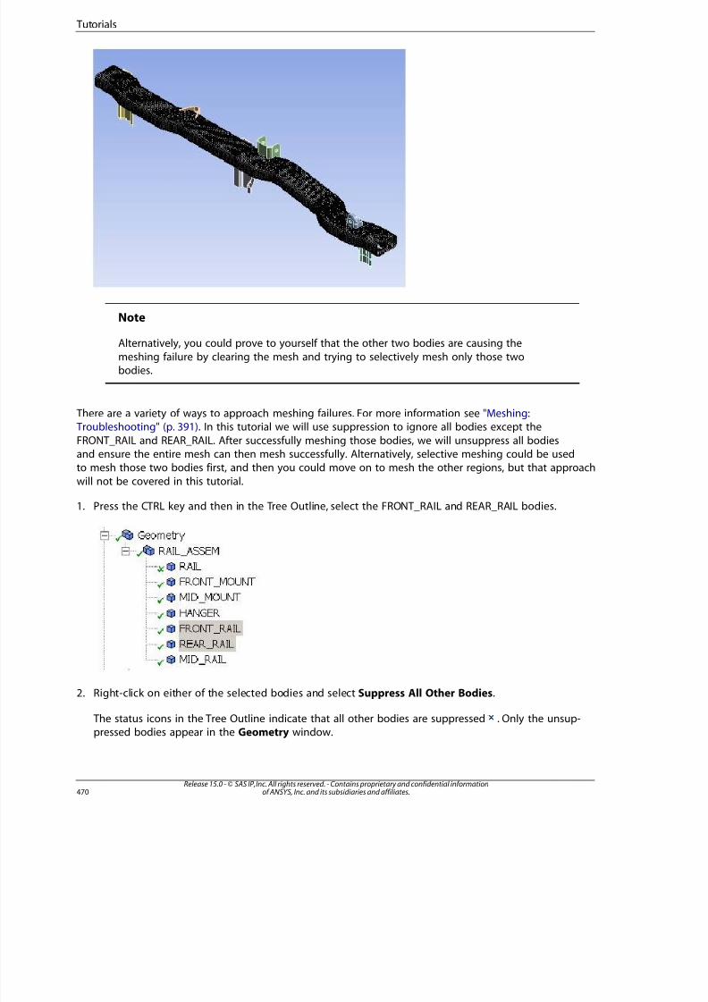
8/10/2019 ANSYS Meshing Users Guide
http://slidepdf.com/reader/full/ansys-meshing-users-guide 478/491
Note
Alternatively, you could prove to yourself that the other two bodies are causing the
meshing failure by clearing the mesh and trying to selectively mesh only those twobodies.
There are a variety of ways to approach meshing failures. For more information see "Meshing: Troubleshooting" (p. 391). In this tutorial we will use suppression to ignore all bodies except the
FRONT_RAIL and REAR_RAIL. After successfully meshing those bodies, we will unsuppress all bodiesand ensure the entire mesh can then mesh successfully. Alternatively, selective meshing could be used
to mesh those two bodies first, and then you could move on to mesh the other regions, but that approachwill not be covered in this tutorial.
1. Press the CTRL key and then in the Tree Outline, select the FRONT_RAIL and REAR_RAIL bodies.
2. Right-click on either of the selected bodies and select Suppress All Other Bodies.
The status icons in the Tree Outline indicate that all other bodies are suppressed . Only the unsup-pressed bodies appear in the Geometry window.
Release 15.0 - © SAS IP, Inc. All rights reserved. - Contains proprietary and confidential informationof ANSYS, Inc. and its subsidiaries and affiliates.470
Tutorials
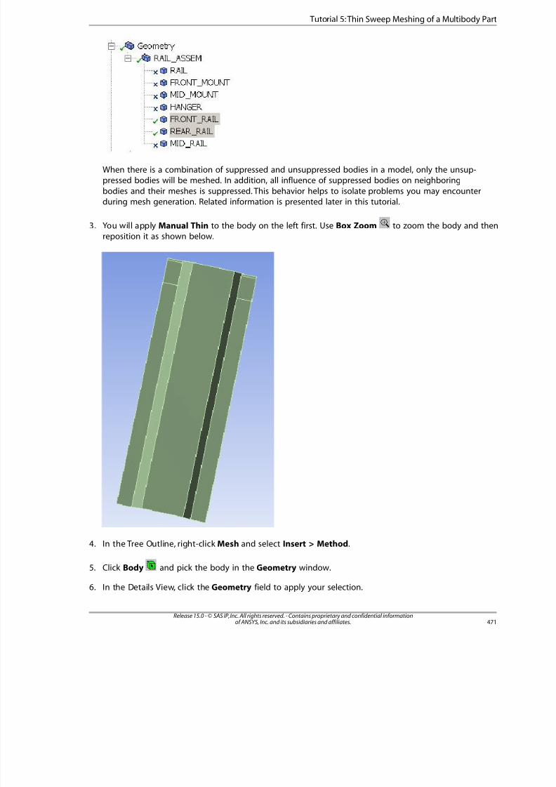
8/10/2019 ANSYS Meshing Users Guide
http://slidepdf.com/reader/full/ansys-meshing-users-guide 479/491
When there is a combination of suppressed and unsuppressed bodies in a model, only the unsup-pressed bodies will be meshed. In addition, all influence of suppressed bodies on neighboring
bodies and their meshes is suppressed. This behavior helps to isolate problems you may encounterduring mesh generation. Related information is presented later in this tutorial.
3. You will apply Manual Thin to the body on the left first. Use Box Zoom to zoom the body and thenreposition it as shown below.
4. In the Tree Outline, right-click Mesh and select Insert > Method.
5. Click Body and pick the body in the Geometry window.
6. In the Details View, click the Geometry field to apply your selection.
47Release 15.0 - © SAS IP, Inc. All rights reserved. - Contains proprietary and confidential informationof ANSYS, Inc. and its subsidiaries and affiliates.
Tutorial 5:Thin Sweep Meshing of a Multibody Part
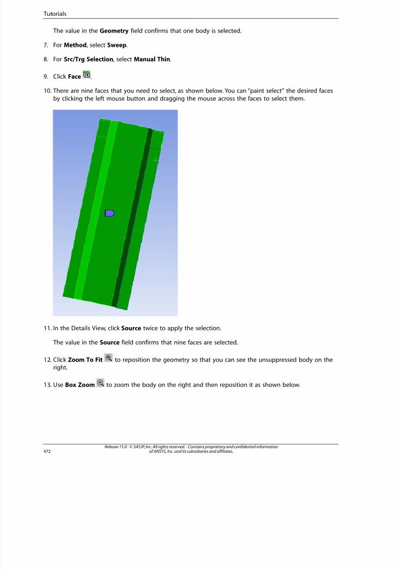
8/10/2019 ANSYS Meshing Users Guide
http://slidepdf.com/reader/full/ansys-meshing-users-guide 480/491
The value in the Geometry field confirms that one body is selected.
7. For Method, select Sweep.
8. For Src/Trg Selection, select Manual Thin.
9. Click Face .
10. There are nine faces that you need to select, as shown below. You can “paint select” the desired facesby clicking the left mouse button and dragging the mouse across the faces to select them.
11. In the Details View, click Source twice to apply the selection.
The value in the Source field confirms that nine faces are selected.
12. Click Zoom To Fit to reposition the geometry so that you can see the unsuppressed body on theright.
13. Use Box Zoom to zoom the body on the right and then reposition it as shown below.
Release 15.0 - © SAS IP, Inc. All rights reserved. - Contains proprietary and confidential informationof ANSYS, Inc. and its subsidiaries and affiliates.472
Tutorials
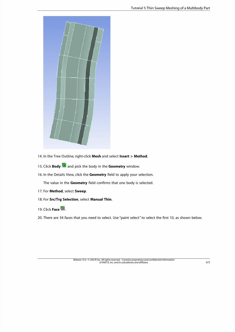
8/10/2019 ANSYS Meshing Users Guide
http://slidepdf.com/reader/full/ansys-meshing-users-guide 481/491
14. In the Tree Outline, right-click Mesh and select Insert > Method.
15. Click Body and pick the body in the Geometry window.
16. In the Details View, click the Geometry field to apply your selection.
The value in the Geometry field confirms that one body is selected.
17. For Method, select Sweep.
18. For Src/Trg Selection, select Manual Thin.
19. Click Face .
20. There are 34 faces that you need to select. Use “paint select” to select the first 10, as shown below.
473Release 15.0 - © SAS IP, Inc. All rights reserved. - Contains proprietary and confidential informationof ANSYS, Inc. and its subsidiaries and affiliates.
Tutorial 5:Thin Sweep Meshing of a Multibody Part
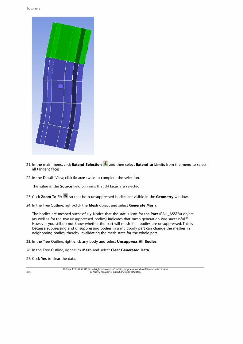
8/10/2019 ANSYS Meshing Users Guide
http://slidepdf.com/reader/full/ansys-meshing-users-guide 482/491
21. In the main menu, click Extend Selection and then select Extend to Limits from the menu to selectall tangent faces.
22. In the Details View, click Source twice to complete the selection.
The value in the Source field confirms that 34 faces are selected.
23. Click Zoom To Fit so that both unsuppressed bodies are visible in the Geometry window.
24. In the Tree Outline, right-click the Mesh object and select Generate Mesh.
The bodies are meshed successfully. Notice that the status icon for the Part (RAIL_ASSEM) object(as well as for the two unsuppressed bodies) indicates that mesh generation was successful .
However, you still do not know whether the part will mesh if all bodies are unsuppressed. This isbecause suppressing and unsuppressing bodies in a multibody part can change the meshes inneighboring bodies, thereby invalidating the mesh state for the whole part.
25. In the Tree Outline, right-click any body and select Unsuppress All Bodies.
26. In the Tree Outline, right-click Mesh and select Clear Generated Data.
27. Click Yes to clear the data.
Release 15.0 - © SAS IP, Inc. All rights reserved. - Contains proprietary and confidential informationof ANSYS, Inc. and its subsidiaries and affiliates.474
Tutorials
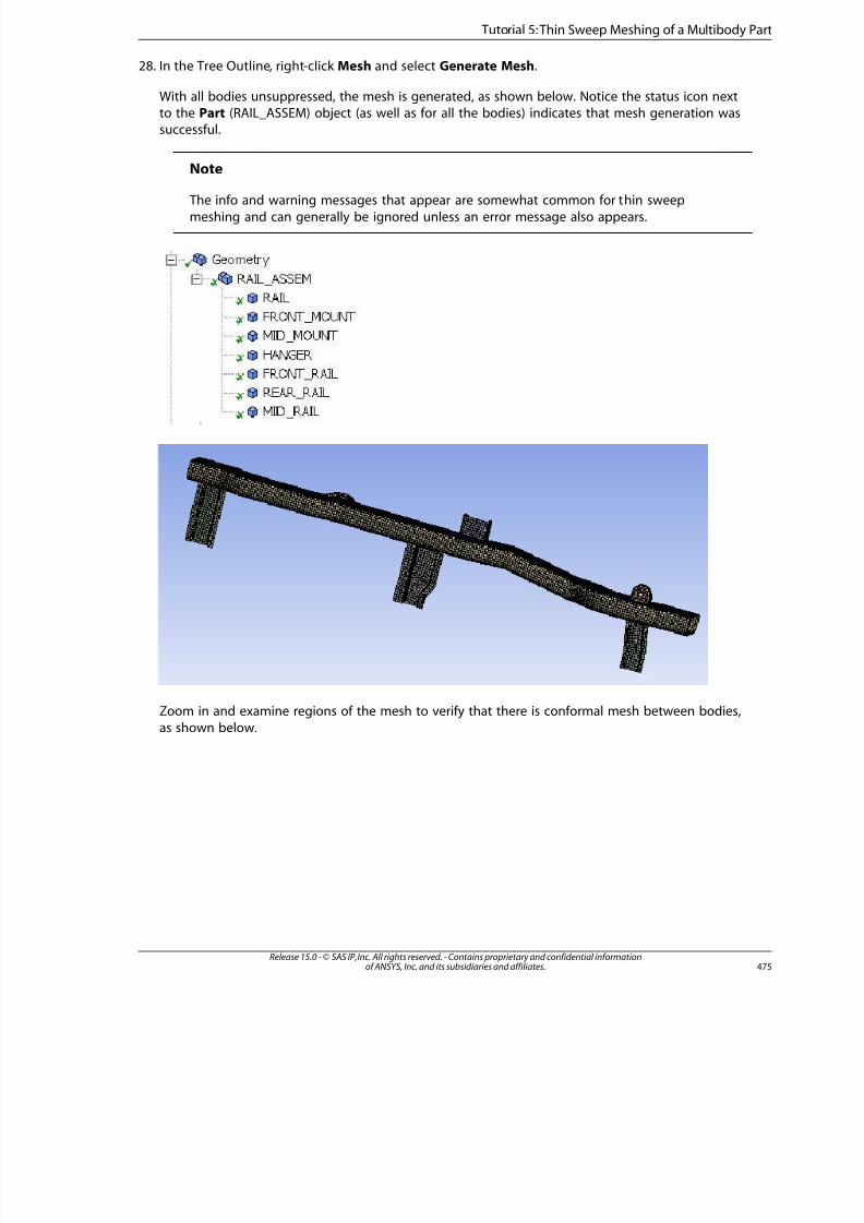
8/10/2019 ANSYS Meshing Users Guide
http://slidepdf.com/reader/full/ansys-meshing-users-guide 483/491
28. In the Tree Outline, right-click Mesh and select Generate Mesh.
With all bodies unsuppressed, the mesh is generated, as shown below. Notice the status icon nextto the Part (RAIL_ASSEM) object (as well as for all the bodies) indicates that mesh generation wassuccessful.
Note
The info and warning messages that appear are somewhat common for thin sweep
meshing and can generally be ignored unless an error message also appears.
Zoom in and examine regions of the mesh to verify that there is conformal mesh between bodies,
as shown below.
475Release 15.0 - © SAS IP, Inc. All rights reserved. - Contains proprietary and confidential informationof ANSYS, Inc. and its subsidiaries and affiliates.
Tutorial 5:Thin Sweep Meshing of a Multibody Part
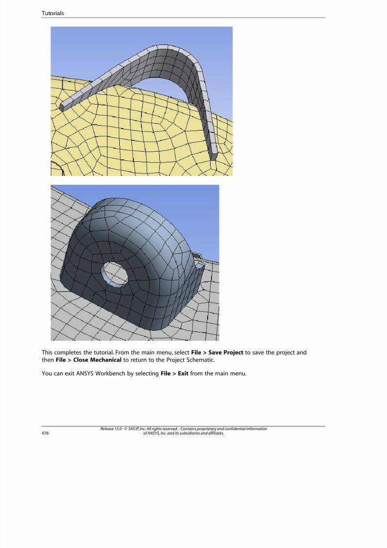
8/10/2019 ANSYS Meshing Users Guide
http://slidepdf.com/reader/full/ansys-meshing-users-guide 484/491
This completes the tutorial. From the main menu, select File > Save Project to save the project andthen File > Close Mechanical to return to the Project Schematic.
You can exit ANSYS Workbench by selecting File > Exit from the main menu.
Release 15.0 - © SAS IP, Inc. All rights reserved. - Contains proprietary and confidential informationof ANSYS, Inc. and its subsidiaries and affiliates.476
Tutorials
8/10/2019 ANSYS Meshing Users Guide
http://slidepdf.com/reader/full/ansys-meshing-users-guide 485/491
Index
Symbols0-thickness walls, 331
A
accessing Meshing functionality, 17activation of Mesh worksheet steps, 311active assembly - initial size seed meshing control op-tion, 77ADF file format, 225
advanced global meshing controls, 104advanced size function - sizing global meshing control,68
curvature,69
fixed, 71influence of, 61proximity, 70
specifying options, 71with specialized meshing, 64
advanced size function tutorial, 451advancing front surface mesher, 100
air gap meshing, 323algorithm
meshing according to, 2
algorithms - tetrahedral meshing algorithms , 147Allow Selective Meshing, 225ANSYS Fluent
input file format, 225
ANSYS Fluent Meshingexporting faceted geometry to, 23
arbitrary match controldescription, 209
ASCII file formatFluent input file format, 225
aspect ratio (base/height) - inflation global meshing
control, 86aspect ratio for quadrilaterals
mesh metric, 129aspect ratio for triangles
mesh metric, 128
assemblies of parts vs. multibody parts, 5assembly meshing, 273
capturing sharp angles, 221
contacts, finding, 298CutCell,97Extend to Connection, 283
Feature Capture, 97finding contacts, 298finding thin sections, 296Fluid Surface object, 283
global meshing controls, 97Intersection Feature Creation, 97
Keep Solid Mesh, 97leak path, 401mesh grouping, 181, 292
Method, 97Morphing Frequency, 97sharp angles, capturing, 221 Tessellation Refinement,97
Tetrahedrons,97thin sections, finding, 296virtual bodies, 283
automatic defeaturing, 120
automatic inflation - inflation global meshing control,80automatic meshing, 61
automatic method - in method control, 147automatic virtual topology, 368auxiliary meshing tools - listed and described, 351
axis sweeping, 169
Bbaffle meshing, 331batch mode, 56
bias (sweeping) - in method control , 169bias factor - in local sizing control, 184bias type - in local sizing control, 184binary file format
Fluent input file format, 225bodies
grouping for meshing, 181, 292
body of influence - local mesh sizing tool option, 184
CCAD instances, 327can combustor tutorial, 409
CFD/fluids meshing strategies,15CFD/fluids meshing with tetrahedrons,217CFX-Mesh method
replacing,21CGNS
file format, 225
version, 225CGNS format export, 23CGNS Version, 225clearing generated data, 363
collision avoidance - inflation global meshing controls90component system
Mesh, 17
conformal meshing, 5mesh method interoperability, 5
477Release 15.0 - © SAS IP, Inc. All rights reserved. - Contains proprietary and confidential informationof ANSYS, Inc. and its subsidiaries and affiliates.

8/10/2019 ANSYS Meshing Users Guide
http://slidepdf.com/reader/full/ansys-meshing-users-guide 486/491
contactsizing - mesh control tool, 193
contact meshing, 323contact sizing
description, 193
contactsfinding for assembly meshing, 298
coordinate systemcreating section planes, 352
crack meshing, 333cracks, 333Create Section Plane, 352curvature normal angle - local mesh sizing tool option,
184curvature normal angle - sizing global meshing control,72
CutCell Cartesian meshingassemblies, 97missing tessellations, 364
orthogonal quality, 138CutCell Cartesian meshing and assemblies, 273
Fluid/Solid material property, 283cyclic match control
description, 208
DDefault Method, 225Default Physics Preference, 225
defaults global meshing controls,65defeaturing
automatic mesh based, 120
defeaturing global meshing controls,109Defeaturing Tolerance, 178defining cracks, 333Delaunay surface mesher, 100
determination of physics, analysis, and solver settings,20dockable worksheet, 311
Eease of use meshing features - listed,353edge behavior - in local sizing control , 184
edge bias - in local sizing control, 184edge splits
using F4 to modify, 374virtual, 374
element midside nodes - advanced global meshingcontrol,106element option
in sweep method mesh control, 169
element qualityfinding worst quality elements, 122
mesh metric, 127element shape
meshing according to, 4element size - local mesh sizing tool option, 184element size - sizing global meshing control, 77
elements - statistics global meshing control, 121exporting - procedure
previewed inflation mesh, 360previewed surface mesh, 357
exporting faceted geometryto ANSYS Fluent Meshing, 23
exporting meshesANSYS Fluent mesh format, 23
ANSYS ICEM CFD format, 23CGNS format, 23Mesh Application File format, 23
overlapping contact regions, 361overlapping Named Selections, 361Polyflow format, 23
Pmeshes, 42Extend to Connection, 283extended ICEM CFD meshing, 55Extra Retries For Assembly, 225
extra retries for assembly - advanced global meshingcontrol , 108
FF4
modifying virtual topology splits, 374, 378face splits
using F4 to modify, 378
virtual, 378File Format, 225Fill Small Holes, 178fillet ratio - inflation global meshing controls , 95
Find Contactsdescription, 298
Find Thin Sectionsdescription, 296
first aspect ratio - inflation global meshing control, 86first layer height - inflation global meshing control, 86Fluent
input file format, 225Fluent mesh export, 23Fluid Surface object, 283Fluid/Solid material property
assembly meshing, 283fluids meshing strategies, 15fluids meshing with tetrahedrons, 217Format of Input File (*.msh), 225
fracture meshing, 333fractures, 333
Release 15.0 - © SAS IP, Inc. All rights reserved. - Contains proprietary and confidential informationof ANSYS, Inc. and its subsidiaries and affiliates.478
Index
8/10/2019 ANSYS Meshing Users Guide
http://slidepdf.com/reader/full/ansys-meshing-users-guide 487/491
Free Mesh Type, MultiZoneHexa Core, 172
Hexa Dominant, 172Not Allowed, 172 Tetra, 172
full assembly - initial size seed meshing control option,77
Ggap tool
description, 222generate pinch on refresh - pinch global meshing con-trol , 115
generating mesh - procedure, 354generating mesh controls from a template,143, 363generation of contact elements,351geometry
vs. topology, 367Geometry window, 18
global meshing settings - listed and defined, 65Graphics window, 18grouping
bodies for meshing, 181, 292growth rate - inflation global meshing control , 86
growth rate - local mesh sizing tool option, 184growth rate - sizing global meshing control, 76growth rate type - inflation global meshing controls ,94
Hhard divisions - in local sizing control, 184hard entities, 329
hard pointsusing in virtual face splits, 378, 381
HDF5 file format, 225hex dominant option - in method control, 168
histogram of mesh metrics, 122history
meshing steps, 311
IICEM CFD
batch mode, 56extended meshing, 55interactive meshing, 55interactive mode, 56writing ICEM CFD files, 56
ICEM CFD mesh export, 23importing meshes
ANSYS CFX, 21ANSYS Fluent, 21
ANSYS ICEM CFD, 21
ANSYS Polyflow, 21imprinting
classifications for MultiZone,258effects on meshing, 5matched vs. non-matched, 5
incremental meshing, 307incremental meshing of bodies, 354inflation advanced options - inflation global meshingcontrols,90
inflation algorithm - inflation global meshing control,87inflation controls
with all triangles mesher,316
with MultiZone, 316with patch conforming mesher, 316with patch independent mesher, 316
with quadrilateral dominant mesher, 316with sweeper, 316
inflation global meshing controls,78
inflation mesh control tool, 217inflation option - inflation global meshing control , 83Inflation options on the Options dialog box, 225initial size seed - sizing global meshing control , 77
inspecting large meshes, 363instances, 327interactions - mesh control, 345interactive ICEM CFD meshing, 55
interactive mode, 56interoperability
mesh method, 5
JJacobian ratio
mesh metric, 130
Llaunching the Meshing application, 17layer compression - inflation global meshing controls,90
leak path, 401legacy data, 21linear elements, 106
local meshing settings - listed and defined, 143loop removal global meshing controls,119loop removal tolerance - loop removal global meshingcontrol, 120
loopsremoving, 362showing removable loops, 362
Mmanual creation of virtual cells, 368
479Release 15.0 - © SAS IP, Inc. All rights reserved. - Contains proprietary and confidential informationof ANSYS, Inc. and its subsidiaries and affiliates.

8/10/2019 ANSYS Meshing Users Guide
http://slidepdf.com/reader/full/ansys-meshing-users-guide 488/491
mapped face meshingdescription, 195
Mapped Mesh Type, MultiZoneHexa, 172Hexa/Prism, 172
Prism, 172master body, 292match control
arbitrary,209
cyclic, 208description, 206
match meshing - and symmetry,324matched vs. non-matched imprinting, 5
max face size - sizing global meshing control , 75max size - sizing global meshing control, 76maximum angle - inflation global meshing controls ,
95maximum corner angle
mesh metric, 135
maximum layers - inflation global meshing control , 85maximum thickness - inflation global meshing control, 86Merge Edges Bounding Manually Created Faces, 225
merge face edges - automatic virtual topology, 368Mesh Application File format export, 23mesh based defeaturing global meshing controls, 120mesh connection, 352
mesh control interaction tables, 345mesh control tools
description, 143instances, 327
patterns, 327precedence,143renaming,352
mesh controls and methods tutorial, 432mesh data
clearing, 363mesh grouping control
description, 181, 292mesh method interoperability, 5mesh metric
histogram, 122
mesh metric - statistics global meshing control , 122aspect ratio for quadrilaterals,129aspect ratio for triangles, 128
element quality, 127Jacobian ratio, 130maximum corner angle, 135orthogonality quality, 138
parallel deviation, 135skewness, 136warping factor, 132
Mesh Metrics bar graph, 122mesh morphing - advanced global meshing control ,
108mesh numbering, 352mesh refinement, 323
mesh sweepinggeneral sweeping, 231thin model sweeping, 238
Mesh system, 17
meshingadvanced size function, 61algorithms - tetrahedral, 147assembly level vs. part/body level, 2
automatic,61auxiliary tools, 351by algorithm, 2
by element shape, 4capabilities in Workbench, 1CFD/fluids,217
clearing generated data, 363conformal meshing, 5control interactions, 345controls,61
determination of physics, analysis, and solver set-tings, 20ease of use features - listed, 353exporting - procedure
previewed inflation mesh, 360previewed surface mesh, 357
fluids, 217generating mesh - procedure, 354
generating mesh controls from a template, 143, 363global controls - listed and defined,65implementation in Workbench, 1
importing meshes, 21inspecting large meshes, 363local mesh controls, 143loop removal, 362
mesh sweepinggeneral sweeping, 231thin model sweeping, 238
Meshing application - basic workflow,11
Meshing application - basic workflow for CFD,12Meshing application - basic workflow for combiningCFD/fluids and structural meshing, 14
Meshing application - basic workflow for Fluids,12Meshing application - description, 11Meshing application - exporting meshes, 23Meshing application - launching, 17
Meshing application - working with legacy meshdata, 21Meshing application interface, 18
Release 15.0 - © SAS IP, Inc. All rights reserved. - Contains proprietary and confidential informationof ANSYS, Inc. and its subsidiaries and affiliates.480
Index
8/10/2019 ANSYS Meshing Users Guide
http://slidepdf.com/reader/full/ansys-meshing-users-guide 489/491
Named Selections, 389non-conformal meshing, 5
optionsexport, 225inflation, 225
meshing,225overview, 225sizing,225virtual topology, 225
overlapping contact regions, 361overlapping Named Selections, 361overview, 1parameters,58
previewing inflation - procedure, 358previewing source and target mesh - procedure,358previewing surface mesh - procedure, 356
replacing a Mesh system with a Mechanical Modelsystem, 18selective, 307, 354
showing geometry in overlapping contact regions -procedure, 361showing geometry in overlapping Named Selections- procedure, 361
showing inflation surfaces - procedure, 360showing mappable faces - procedure, 365showing missing tessellations, 364showing problematic geometry - procedure,361
showing removable loops, 362showing sweepable bodies - procedure,360specialized - 0-thickness walls, 331specialized - air gap meshing,323
specialized - assembly, 273specialized - baffle meshing, 331specialized - CAD instance, 327
specialized - contact meshing, 323specialized - cracks, 333specialized - fracture, 333specialized - hard entities, 329
specialized - inflation controls,316specialized - listed, 231specialized - match meshing and the symmetryfolder, 324
specialized - mesh refinement, 323specialized - mixed order meshing, 323specialized - MultiZone, 251
specialized - non-manifold faces, 331specialized - pyramid transitions, 324specialized - rigid body contact meshing,324specialized - rigid body meshing, 324
specialized - spot weld, 329specialized - sweeping, 231specialized - thin solid meshing,327
specialized - winding body meshing, 324specialized - wire body meshing, 324
troubleshooting,391tutorials,409
advanced size function, 451
can combustor, 409mesh controls and methods, 432single body inflation, 418thin sweep meshing of a multibody part, 466
types - listed, 2updating the Mesh cell state - procedure,353Workbench vs. Mechanical APDL, 59workflow, 1
workflow - basic meshing, 11workflow - CFD meshing, 12workflow - combining CFD/fluids and structural
meshing, 14workflow - Fluids meshing, 12
Meshing application
basic meshing workflow, 11basic workflow, 11basic workflow for CFD, 12basic workflow for fluids, 12
combining CFD/fluids meshing and structuralmeshing, 14description, 11determination of physics, analysis, and solver set-
tings, 20interface overview, 18strategies for CFD/fluids meshing, 15tutorials,409
advanced size function, 451can combustor, 409mesh controls and methods, 432
single body inflation, 418thin sweep meshing of a multibody part, 466
meshing support for hard entities, 329meshing support for pattern instances, 327
meshing support for spot welds,329method mesh control tool
description, 144interactions - MultiZone quad/tri, 345
midside nodesadvanced global control setting, 106method control setting, 144
mixed order meshing, 144min size - sizing global meshing control, 74minimum edge length - sizing global meshing contro, 78
mixed order meshing, 144, 323multibody parts vs. assemblies of parts, 5MultiZone,251
48Release 15.0 - © SAS IP, Inc. All rights reserved. - Contains proprietary and confidential informationof ANSYS, Inc. and its subsidiaries and affiliates.
8/10/2019 ANSYS Meshing Users Guide
http://slidepdf.com/reader/full/ansys-meshing-users-guide 490/491
Free Mesh TypeHexa Core, 172
Hexa Dominant, 172Not Allowed, 172 Tetra, 172
imprinting classifications, 258Mapped Mesh Type
Hexa, 172Hexa/Prism,172
Prism, 172MultiZone option - in method control, 172MultiZone quad/tri mesh control interactions, 345MultiZone quad/tri option - in method control, 178
NNamed Selections
and regions for CFX applications, 389
exporting faceted geometry to TGrid,23inspecting large meshes, 363
program controlled inflation and, 81sending to solver, 352
nodes - statistics global meshing control, 121non-conformal meshing, 5non-manifold faces, 331
num cells across gap - sizing global meshing control ,72Number of CPUs for Meshing Methods, 225Number of CPUs for Parallel Part Meshing, 225
number of layers - inflation global meshing control , 86Number of Retries, 225number of retries - advanced global meshing control ,
107
OObject Generator
using to generate mesh controls,143, 363
Options dialog boxexport, 225inflation, 225
meshing,225overview, 225sizing, 225
virtual topology, 225orthogonal quality
mesh metric, 138overriding of mesh control tools, 143
Pparallel deviation
mesh metric, 135Parameter Workspace
Meshing application and, 58
parametersMeshing application and, 58
part - initial size seed meshing control option, 77patch conforming options
advancing front surface mesher, 100
Delaunay surface mesher, 100global meshing controls, 100 Triangle Surface Mesher,100
patch conforming tetrahedral meshing algorithm , 147
patch independent controls, 101patch independent tetrahedral meshing algorithm ,148
missing tessellations, 364
patterns, 327persistence
meshing steps, 311
physics preference default global meshing control , 65pinch control
defining pinch control automation, 109
defining pinch controls locally,211defining pinch controls manually,211post, 109, 211pre, 109, 211
snap to boundary, 211pinch global meshing controls, 109pinch tolerance - pinch global meshing control , 114Pmeshes, 42
Polyflow format export, 23Pmeshes, 42
Polyflow import, 21post inflation - inflation global meshing control, 87
pre inflation - inflation global meshing control, 87precedence of mesh control tools,143previewing inflation - procedure, 358
previewing source and target mesh - procedure, 358previewing surface mesh - procedure,356problematic geometry, 361program controlled inflation, 81
projecting nodes to underlying geometry,368proximity min size - sizing global meshing control, 75proximity size function sources - sizing global meshingcontrol, 72
pyramid transitions, 324
Qquadratic elements, 106
quadrilateral dominant option - in method control , 178quality metrics, 122
Rrecording
selective meshing steps, 311
Release 15.0 - © SAS IP, Inc. All rights reserved. - Contains proprietary and confidential informationof ANSYS, Inc. and its subsidiaries and affiliates.482
Index
8/10/2019 ANSYS Meshing Users Guide
http://slidepdf.com/reader/full/ansys-meshing-users-guide 491/491
refinement,323description, 194
Relevance,225relevance center - sizing global meshing control , 76relevance default global meshing control, 67
removing loops, 362renaming mesh control tool, 352replacing a Mesh system with a Mechanical Model sys-tem, 18
replacing CFX-Mesh method, 21rigid body behavior - advanced global meshing control,108rigid body contact meshing, 324
rigid body meshing, 324
Ssection planes
creating, 352selective meshing, 307, 354
adding steps manually,311history, 311Mesh worksheet, 311recording steps, 311
Send to Solver, 352
shape checking - advanced global meshing control ,
Snap Type, 211soft divisions - in local sizing control , 184
solver preference default global meshing control , 67span angle center - sizing global meshing control , 78specialized meshing, 231
sphere of influence - local mesh sizing tool option, 184splitting
edges, 374faces, 378
spot welds, 329stair stepping - inflation global meshing controls, 90statistics
quality, 122
virtual topology, 388statistics global meshing controls, 121straight sided elements - advanced global meshing
control, 107strategies
assembly meshing, 273
strategies for CFD/fluids meshing,15sweep option - in method control, 169sweeping - mesh
general sweeping, 231
thin model sweeping, 238symmetry - and match meshing, 324