Anomaly detection and root cause diagnosis in cellular ...
173
HAL Id: tel-02304602 https://tel.archives-ouvertes.fr/tel-02304602 Submitted on 3 Oct 2019 HAL is a multi-disciplinary open access archive for the deposit and dissemination of sci- entific research documents, whether they are pub- lished or not. The documents may come from teaching and research institutions in France or abroad, or from public or private research centers. L’archive ouverte pluridisciplinaire HAL, est destinée au dépôt et à la diffusion de documents scientifiques de niveau recherche, publiés ou non, émanant des établissements d’enseignement et de recherche français ou étrangers, des laboratoires publics ou privés. Anomaly detection and root cause diagnosis in cellular networks Maha Mdini To cite this version: Maha Mdini. Anomaly detection and root cause diagnosis in cellular networks. Artificial Intelligence [cs.AI]. Ecole nationale supérieure Mines-Télécom Atlantique, 2019. English. NNT: 2019IMTA0144. tel-02304602
Transcript of Anomaly detection and root cause diagnosis in cellular ...
HAL Id: tel-02304602https://tel.archives-ouvertes.fr/tel-02304602
Submitted on 3 Oct 2019
HAL is a multi-disciplinary open accessarchive for the deposit and dissemination of sci-entific research documents, whether they are pub-lished or not. The documents may come fromteaching and research institutions in France orabroad, or from public or private research centers.
L’archive ouverte pluridisciplinaire HAL, estdestinée au dépôt et à la diffusion de documentsscientifiques de niveau recherche, publiés ou non,émanant des établissements d’enseignement et derecherche français ou étrangers, des laboratoirespublics ou privés.
Anomaly detection and root cause diagnosis in cellularnetworksMaha Mdini
To cite this version:Maha Mdini. Anomaly detection and root cause diagnosis in cellular networks. Artificial Intelligence[cs.AI]. Ecole nationale supérieure Mines-Télécom Atlantique, 2019. English. NNT : 2019IMTA0144.tel-02304602

THESE DE DOCTORAT DE
L’ÉCOLE NATIONALE SUPERIEURE MINES-TELECOM ATLANTIQUE
BRETAGNE PAYS DE LA LOIRE - IMT ATLANTIQUE
COMUE UNIVERSITE BRETAGNE LOIRE
ECOLE DOCTORALE N° 601 Mathématiques et Sciences et Technologies de l'Information et de la Communication Spécialité : Informatique
ANOMALY DETECTION AND ROOT CAUSE DIAGNOSIS IN CELLULAR NETWORKS Thèse présentée et soutenue à Rennes, le 20/09/2019 Unité de recherche : IRISA
Thèse N° : 2019IMTA0144
(8)
Par
Maha Mdini
Rapporteurs avant soutenance : M. Damien Magoni Professeur, Université de Bordeaux M. Pierre Parrend Professeur, ECAM Strasbourg
Composition du Jury : Président : M. Eric Fabre Directeur de recherche, INRIA Rennes Examinateurs : M. Damien Magoni Professeur, Université de Bordeaux M. Pierre Parrend Professeur, ECAM Strasbourg Mme. Lila Boukhatem Maitre de conférences, Université de Paris XI M. Alberto Blanc Maitre de conférences, IMT Atlantique Directeur de thèse : M. Gwendal Simon Professeur, IMT Atlantique

Maha Mdini: Anomaly Detection and Root Cause Diagnosisin Cellular Networks, PhD Thesis, © October 2, 2019
[ October 2, 2019 – Anomaly Detection and Root Cause Analysis v1.0 ]

To my beloved family,Mariem and Hedi,
Houda and Mohamed,Jawher,
and Ahlem.
[ October 2, 2019 – Anomaly Detection and Root Cause Analysis v1.0 ]

[ October 2, 2019 – Anomaly Detection and Root Cause Analysis v1.0 ]

A B S T R A C T
With the evolution of automation and artificial intelligence tools, mobile networks havebecome more and more machine reliant. Today, a large part of their management tasksruns in an autonomous way, without human intervention. The latest standards of theThird Generation Partnership Project (3GPP) aim at creating Self-Organizing Network(SON) where the processes of configuration, optimization and healing are fully auto-mated. This work is about the healing process. This question have been studied bymany researchers. They designed expert systems and applied Machine Learning (ML)algorithms in order to automate the healing process. However this question is still notfully addressed. A large part of the network troubleshooting still rely on human experts.For this reason, we have focused in this thesis on taking advantage of data analysis toolssuch as pattern recognition and statistical approaches to automate the troubleshootingtask and carry it to a deeper level. The troubleshooting task is made up of three pro-cesses: detecting anomalies, analyzing their root causes and triggering adequate recov-ery actions. In this document, we focus on the two first objectives: anomaly detectionand root cause diagnosis.
The first objective is about detecting issues in the network automatically without in-cluding expert knowledge. To meet this objective, we have created an Anomaly Detec-tion System (ADS) that learns autonomously from the network traffic and detects anoma-lies in real time in the flow of data. The algorithm we propose, Watchmen AnomalyDetection (WAD), is based on pattern recognition. It learns patterns from periodic timeseries and detect distortions in the flow of new data. We have assessed the performanceof our solution on different data sets and WAD has been proven to provide accurate re-sults. In addition, WAD has a low computational complexity and very limited memoryneeds. WAD has been industrialized and integrated in two commercialized products tofill the functions of supervising monitoring systems and managing service quality.
The second objective is automatic diagnosis of network issues. This project aimsat identifying the root cause of issues without any prior knowledge about the net-work topology and services. To address this question, we have designed an algorithm,Automatic Root Cause Diagnosis (ARCD) that identifies the roots of network issues. ARCD
is composed of two independent threads: Major Contributor identification and Incom-patibility detection. Major contributor identification is the process of determining theelements (devices, services and users) that are causing the overall efficiency of the net-work to drop significantly. These elements have inefficiency issues and contribute to anon-negligible amount of the traffic. By troubleshooting these issues, the network perfor-mance increases significantly. The second process, incompatibility detection, deals withmore fine and subtle type of issues. An incompatibility is an inefficient combination ofefficient elements. Incompatibilities cannot be diagnosed by human experts in a reason-able amount of time. We have tested the performance of ARCD and the obtained resultsare satisfactory. An integration of ARCD in a commercialized troubleshooting product isongoing and the first results are promising.
v
[ October 2, 2019 – Anomaly Detection and Root Cause Analysis v1.0 ]

WAD and ARCD have been proven to be effective. However, many improvements ofthese algorithms are possible. This thesis does not address fully the question of self-healing networks. Nevertheless, it contributes to the understanding and the implemen-tation of this concept in production cellular networks.
vi
[ October 2, 2019 – Anomaly Detection and Root Cause Analysis v1.0 ]
R É S U M É
Grâce à l'évolution des outils d'automatisation et d'intelligence artificielle, les réseauxmobiles sont devenus de plus en plus dépendants de la machine. De nos jours, unegrande partie des tâches de gestion de réseaux est exécutée d'une façon autonome,sans intervention humaine. Les dernières normes de la Third Generation PartnershipProject (3GPP) visent à créer des réseaux dont l'organisation est autonome (Self-OrganizingNetwork (SON)). Dans ces réseaux, les procédures de configuration, d'optimisation et derestauration (healing) sont entièrement automatisées. Ce document a pour objet l'étudedu processus de restauration. Dans cette thèse, nous avons focalisé sur l'utilisation destechniques d'analyse de données dans le but d'automatiser et de consolider le processusde résolution de défaillances dans les réseaux. Pour ce faire, nous avons défini deuxobjectifs principaux: la détection d'anomalies et le diagnostic des causes racines de cesanomalies (root cause diagnosis).
Le premier objectif consiste à détecter automatiquement les anomalies dans lesréseaux sans faire appel aux connaissances des experts. Pour atteindre cet objectif, nousavons créé un système autonome de détection d'anomalies qui extrait de l'informationdu trafic réseau et détecte les anomalies en temps réel dans le flux de données.L'algorithme qu'on propose, Watchmen Anomaly Detection (WAD), est basé sur le conceptde la reconnaissance de formes (pattern recognition). Cet algorithme apprend le modèledu trafic réseau à partir de séries temporelles périodiques et détecte des distorsions parrapport à ce modèle dans le flux de nouvelles données. Nous avons évalué les perfor-mances de notre solution sur des données venant de différents réseaux. Les résultatsfournis par WAD font preuve de précision. Outre cela, WAD est efficace en termes detemps d'exécution et d'utilisation d'espace mémoire. Nous avons intégré WAD dans deuxproduits commercialisés pour contrôler les systèmes de supervision (monitoring systems)ainsi que pour gérer la qualité de service.
Le second objectif de la thèse est le diagnostic des causes racines. Ce projet a pourbut la détermination des causes racines des problèmes réseau sans aucune connaissancepréalable sur l'architecture du réseau et des différents services. Pour ceci, nous avonsconçu un algorithme, Automatic Root Cause Diagnosis (ARCD), qui permet de localiser lessources d'inefficacité dans le réseau. ARCD est composé de deux processus indépendants:l'identification des contributeurs majeurs à l'inefficacité globale du réseau et la détectiondes incompatibilités. L'identification des contributeurs majeurs consiste à déterminerles éléments (équipements, services et utilisateurs) qui sont à l'origine d'une chute im-portante de l'efficacité globale du réseau. Ces éléments ont une faible performance etcontribuent à une quantité de trafic non négligeable. En résolvant ces défaillances, lesperformances du réseau augmentent considérablement. La détection des incompatibil-ités traite des problèmes plus fins. Une incompatibilité est un ensemble d'éléments fonc-tionnels dont la combinaison est non fonctionnelle. Les incompatibilités ne peuvent pasêtre identifiées par un expert en un délai raisonnable. Nous avons testé les performancesd'ARCD et les résultats qu'on a obtenus sont satisfaisants. L'intégration d'ARCD dans un
vii
[ October 2, 2019 – Anomaly Detection and Root Cause Analysis v1.0 ]

produit commercialisé de diagnostic de réseau est en cours et les premiers résultats detests sont prometteurs.
WAD et ARCD ont fait preuve d'efficacité. Cependant, il est possible d'améliorer cesalgorithmes sur plusieurs aspects. Cette thèse ne donne pas une réponse complète àla question de l'auto-restauration (self-healing) dans les réseaux. Néanmoins, elle con-tribue à la compréhension et l'implémentation de ce concept dans les réseaux mobilesopérationnels. Dans ce qui suit, nous décrivons le fonctionnement de WAD et d'ARCD.
la détection d 'anomalies
Nous avons créé une solution de détection d'anomalies qui permet d'identifier les prob-lèmes survenant dans un système de supervision en temps réel et d'une façon dy-namique. Le but du WAD est de détecter des changements brusques tels que les crêteset les creux dans des séries temporelles périodiques. Ces anomalies peuvent provenirde problèmes de configuration, de pannes d'équipements conduisant à une perte detrafic réseau, d'évènements de masse (tels que les évènements sportifs) à l'origine d'unesaturation d'équipements, etc.
Notre solution doit répondre à un ensemble d'exigences spécifiées par les utilisateursfinaux de la solution qui sont les administrateurs systèmes et les techniciens réseaux.En premier lieu, la solution doit être facile à mettre en place, à configurer et à piloter.Deuxièmement, contrairement aux méthodes basées sur des seuils fixes, cette solutiondoit s'appliquer à des données périodiques. De plus, le modèle généré par l'algorithmedoit être ajusté dynamiquement pour refléter l'évolution naturelle du trafic. La solutiondoit être aussi proactive pour détecter les anomalies en temps réel. En outre, la solutiondoit être non supervisée: Elle ne doit nécessiter aucun effort humain une fois déployée.La configuration doit être facile. En d'autres termes, la solution doit inclure un nombreréduit de paramètres pouvant facilement être compris et modifiés par les utilisateursfinaux. Outre cela, le but principal de la solution est d'avoir un taux de détection prochede 100% avec un faible taux de faux positifs. Enfin, et ce n'est pas le point le moinsimportant, il est primordial que l'algorithme ait une complexité faible pour que le tempsde calcul ainsi que les ressources requises soient raisonnables.
WAD répond aux exigences citées précédemment en analysant des métriques collectéespar le système de supervision. Ces métriques peuvent être le débit du trafic en entréedes sondes, le nombre de comptes rendus de communication (Call Data Record (CDR) etSession Data Record (SDR)) en entrée/sortie des équipements de supervisions, le taux dedéchiffrement, etc. Ces métriques forment des séries temporelles unidimensionnelles etsont fortement corrélées avec le comportement des abonnées. Ainsi, elles présentent unepériodicité journalière avec des pics autour de 12h et 18h.
Pour chaque métrique, WAD génère un modèle de référence (pattern) décrivantl'évolution normale du trafic. Ensuite, il mesure l'écart entre le modèle de référenceet les données temps réel. Si l'écart excède le seuil calculé, une alerte est déclenchée au-tomatiquement pour prévenir les administrateurs réseaux de l'apparition d'une anoma-lie. WAD comprend deux phases: une phase d'apprentissage et une phase de détection.La phase d'apprentissage est exécutée une seule fois par jour dans le cas d'une péri-odicité journalière. Dans cette phase, WAD crée un modèle de référence pour chaquemétrique et le stocke dans une base de données. Ce modèle sera utilisé durant la phase
viii
[ October 2, 2019 – Anomaly Detection and Root Cause Analysis v1.0 ]
de détection, qui s'exécute en continu. Avant de lancer l'algorithme, une étape de pré-traitement (preprocessing) est exécutée dans le but de compléter les valeurs manquanteset de normaliser l'intervalle de temps entre les échantillons consécutifs. Pour ce faire,nous appliquons simplement une interpolation linéaire.
Vu qu'on ne s'intéresse qu'aux données périodiques, la phase d'apprentissage com-mence par un test de la périodicité des donnés. Pour ce faire, nous appliquons laTransformée de Fourier dans le but d'identifier une fréquence dominante. Si une tellefréquence a été détectée, on peut affirmer que la métrique est périodique et que sa péri-ode est égale à l'inverse de la fréquence dominante. Dans ce cas, nous passons à l'étapesuivante du WAD qui est le calcul du modèle de référence. Ce calcul se fait en deuxtemps. Dans un premier temps, on segmente l'historique de la métrique en périodes eton calcule la moyenne point à point de toutes les périodes. Cette moyenne présente unmodèle de référence provisoire. On écarte ensuite toutes les valeurs extrêmes par rap-port à ce modèle et on recalcule la moyenne point à point. Cette moyenne représentele modèle de référence final de la métrique. Cette méthode nous permet d'obtenir unmodèle de référence non biaisé par les valeurs extrêmes. Nous appliquons, par la suite,une transformation que l'on appelle Difference over Minimum (DoM) caractérisant les vari-ations de la métrique durant une période. Cette transformée permet d'amplifier les vari-ations brusques et de réduire les variations de faible amplitude. Cette transformée estappliquée également à l'historique des données. En étudiant la distribution de la trans-formée DoM des données autour de la transformée du modèle de référence, on calculeun seuil de normalité au delà duquel un échantillon est considéré comme très différentdu modèle de référence et par la suite anormal. Le modèle de référence et le seuil calculésont stockés dans la base de données.
Durant la phase de détection, on compare les échantillons arrivant dans le flux dedonnées au modèle de référence construit durant la phase d'apprentissage. Si l'écart dé-passe le seuil calculé durant la phase d'apprentissage, les nouvelles données présententdes anomalies. Pour ce faire, on applique la transformée DoM aux échantillons arrivantdans le flux de données. Après, on calcule la distance euclidienne entre la transforméede l'échantillon et la transformée du modèle de référence qu'on extrait de la base dedonnées. Si cette distance est supérieure à la valeur du seuil calculé durant la phased'apprentissage, une alerte est déclenchée. Le modèle de référence et le seuil sont mis àjour en début de chaque période lors de l'exécution de la phase d'apprentissage.
Nous avons évalué les performances de WAD en utilisant des données provenant dedifférents réseaux d'opérateurs. Nous avons comparé les performances de WAD à deuxalgorithmes de référence qui sont Symbolic Aggregate Approximation (SAX) et PrincipalComponent Analysis (PCA). Pour appliqer la PCA qui exige des données multidimension-nelles, nous avons transformé les séries temporelles unidimensionnelles à des sériesmultidimensionnelles en introduisant des décalages temporels. Dans notre contexte oùon traite des séries temporelles collectées par un système de supervision, WAD est le seulparmi les algorithmes testés à offrir un bon compromis entre le taux de détection et laprécision.
WAD a été industrialisé et déployé dans des réseaux opérationnels en tant que pluginde détection d'anomalies dans deux produits commercialisés d'EXFO. Les techniciensréseaux ont confirmé que WAD leur a permis de gagner en temps et en productivité etleur a facilité la tâche de dépannage du réseau. En effet, WAD automatise l'analyse répéti-
ix
[ October 2, 2019 – Anomaly Detection and Root Cause Analysis v1.0 ]

tive des métriques de supervision, effectuée manuellement par les experts. La précisionet la réactivité de cet outil confirme l'avantage de l'utilisation du Machine Learning dansles réseaux mobiles.
le diagnostic des causes racines
La structure des réseaux mobiles est très complexe. Les opérateurs interfacent des tech-nologies différentes (3G, 4G et 5G). Les équipements utilisés viennent de différents con-structeurs. Les services proposés par les fournisseurs d'accès sont très variés. Les abon-nés utilisent des téléphones différents avec des systèmes d'exploitation variés. Ces faitscomplexifie le diagnostic des réseaux et la détermination des causes racines des prob-lèmes. Dans leur analyse, les opérateurs se basent sur les comptes rendus de commu-nication pour expliquer les problèmes réseaux. Un compte rendu trace les équipementsréseaux impliqués dans la communication, la nature et les caractéristiques du servicerequêté ainsi que des données liées à l'abonné tel que le type du téléphone utilisé dansla requête. Grâce à ces informations, les experts sont capables de déterminer l’originedes problèmes survenus. Cependant, cette analyse telle que faite aujourd'hui est trèsfastidieuse. Elle demande une grande expertise, du temps et un effort important de lapart des experts. Pour cette raison, des recherches ont été menées pour automatiser cettetâche. Cependant, ces propositions ne répondent pas complètement à cette question.
La solution qu'on propose doit répondre à plusieurs contraintes. En premier lieu,elle doit être applicable à différents types de communications tels que les appelsvoix et les connections Transmission Control Protocol (TCP). Deuxièmement, la solutiondoit s'appliquer à des données ayant un nombre de dimensions très élevé. Actuelle-ment, le nombre dimensions d'un CDR peut être supérieur à 100. Ces dimensionssont hétérogènes. On peut distinguer des dimensions de type réseau (les équipementsréseaux), des dimensions de types service tels que le type du service ou l'identifiantdu fournisseur et des dimensions de types abonné tels que le type du téléphone et laversion du système d'exploitation. La solution doit prendre en considération les dépen-dances entre différentes dimensions. Ces dépendances sont expliquées par l'architecturedu réseaux et des différents services. Outre cela, un problème réseaux n'est pas forcé-ment expliqué par un seul élément mais pourrait résulter d'une combinaison d'élémentscomme dans le cas des incompatibilités. Enfin, notre solution doit hiérarchiser les dif-férents problèmes selon leurs impacts et ne retourner que les plus pertinents.
On peut résumer les objectifs de notre solution, ARCD en trois points. Le premier pointconcerne l'identification des contributeurs majeurs. On appelle contributeur majeur toutélément à l'origine d'une baisse importante de l'efficacité globale du réseau. Par exem-ple, un Mobility Management Entity (MME) non fonctionnel peut bloquer la transmissiond'un grand nombre d'appels. Une fois identifiés, les contributeurs majeurs peuvent êtredépannés par des experts. Le deuxième point concerne la détection des incompatibil-ités. Une incompatibilité est un ensemble d'éléments fonctionnels lorsqu'ils sont prisséparément et non fonctionnels quand ils sont combinés. Citons à titre d'exemple uneversion d'un système d'exploitation incompatible avec un service à cause d'un bug dansl'implémentation de ce service. Le dernier objectif de notre solution est la création declasses d'équivalence. Une classe d'équivalence est un ensemble d'éléments liés au mêmeproblème. La corrélation des éléments d'une même classe d'équivalence peut provenir
x
[ October 2, 2019 – Anomaly Detection and Root Cause Analysis v1.0 ]

de l'architecture du réseau. Après avoir identifié les contributeurs majeurs et les incom-patibilités, une analyse statistique des dépendances nous permet de créer différentesclasses d'équivalence. L'étude de ces classes nous permet de réduire chaque problème àsa cause racine.
La détermination des contributeurs majeurs se fait en cinq étapes. On commence parla labellisation des comptes rendus de communication s'ils ne sont pas labellisés. Pourceci, on se base sur des critères liés à la qualité de service. Par exemple, si le tempsde réponse est supérieur à un seuil minimal, on considère que la connexion a échoué.Après, on identifie les éléments qui sont suffisamment présents dans les comptes ren-dus des communications échoués et le sont beaucoup moins dans les communicationscorrectement abouties. Pour ce faire, nous avons créé un système de classement (scor-ing system) qui permet d'identifier les éléments les plus importants. Par la suite, ceséléments sont groupés dans des classes d'équivalence. Une classe d'équivalence est unensemble d'éléments impliqués dans les mêmes communications. On explore, ensuite,les dépendances hiérarchiques entre différentes classes d'équivalence et on produit ungraphe de dépendances. Pour créer le graphe, on connecte les classes selon leurs dépen-dances hiérarchiques. Pour rendre le graphe lisible et exploitable, on supprime les lienssuperflus entre les nœuds (les liens qui portent une information redondante). Pour ceci,on utilise l'algorithme de parcours en profondeur pour déterminer tous les chemins pos-sibles entre nœuds et on ne garde que le chemin le plus long. En utilisant cette méthode,on supprime les redondances tout en gardant la totalité de l'information. On termine parl'élagage du graphe de façon à ne garder que les causes racines des problèmes réseaux.
Pour identifier les incompatibilités, on procède en six étapes. On commence par la la-bellisation des comptes rendus de communication s'ils ne sont pas labellisés. Après, onparcourt tous les comptes rendus de communication pour identifier les combinaisons dedeux éléments incompatibles. En d'autres termes, on cherche les éléments qui ont cha-cun un taux d'échec global faible, mais dont la combinaison a un taux d'échec important.L'étape suivante consiste à écarter les fausses incompatibilités. Une fausse incompatibil-ité est une combinaison ayant un taux d'échec important. Cependant, ce taux d'échecest expliqué par la présence d'un troisième élément non fonctionnel dans les comptesrendus contenant la combinaison. Par la suite, pour chaque élément présent les com-binaisons restantes, on identifie l'ensemble d'éléments qui sont incompatibles avec lui.Puis, on groupe ces éléments dans des classes d'équivalence. Comme pour les contribu-teurs majeurs, on crée un graphe de dépendance et on procède à l'élagage pour negarder que les racines des incompatibilités.
Nous avons évalué les performances d'ARCD dans la détermination des contributeursmajeurs et des incompatibilités. Les résultats sont prometteurs. Nous avons testé notresolution sur des données réelles venant de trois opérateurs différents. Avec les deuxprocessus de détection de contributeurs majeurs et d'incompatibilités, nous avons puexpliquer respectivement 95%, 96% et 72% des échecs d'appels et de connexions TCP
rencontrés par les abonnés des trois opérateurs. La précision dans le diagnostic des con-tributeurs majeurs est supérieure à 0.9 dans les trois cas et celle des incompatibilités estsupérieure à 0.86. Nous avons comparé ARCD avec l'algorithme Learning from ExamplesModule, version 2 (LEM2) et nous avons conclu qu'ARCD est plus performant en termesde précision et de couverture de problèmes. ARCD est en cours d'industrialisation pourêtre intégré dans une solution d'analyse de performance de réseaux. ARCD sera aussi
xi
[ October 2, 2019 – Anomaly Detection and Root Cause Analysis v1.0 ]

connecté à WAD pour que le processus de détection d'anomalies déclenche automatique-ment le diagnostic des causes racines.
xii
[ October 2, 2019 – Anomaly Detection and Root Cause Analysis v1.0 ]

P U B L I C AT I O N S
M.Mdini, G.Simon, A.Blanc, and J.Lecoeuvre. Automatic Root Cause Diagnosis in Telecommu-nication Networks. Patent Pending, 2018.
M.Mdini, G.Simon, A.Blanc, and J.Lecoeuvre, ARCD: a Solution for Root Cause Diagnosisin Mobile Networks, in CNSM, 2018.
M.Mdini, A.Blanc, G.Simon, J.Barotin, and J.Lecoeuvre, Monitoring the Network MonitoringSystem: Anomaly Detection using Pattern Recognition, in IM, 2017.
xiii
[ October 2, 2019 – Anomaly Detection and Root Cause Analysis v1.0 ]

[ October 2, 2019 – Anomaly Detection and Root Cause Analysis v1.0 ]

A C K N O W L E D G E M E N T S
I would like to thank, first and foremost, Professor Gwendal Simon and Professor Al-berto Blanc without whom this thesis could not be done. During three years, they wereguiding me through each step of the PhD and supporting me with every single task Ihad to accomplish. I am grateful to them for their help with the design and the valida-tion of technical solutions. I would also thank them for their patience while reviewingand correcting my documents. I have learned a lot from their technical knowledge andpersonal qualities and I feel honored for the great opportunity I had to work with them.I would like also to thank IMT Atlantique for opening its doors to me for both myengineering degree and my PhD.
I had also the privilege to conduct my PhD in EXFO, the company which offered theperfect environment for this work. I would like to thank the members of my team,especially, Mr. Sylvain Nadeau, Mr. Loïc Le Gal and Mr. Jérôme Thierry for their supportand help during these three years. I could not forget to thank Mr. Julien Lecoeuvre andMr. Jérôme Barôtin with whom I worked during the first part of my PhD. I am alsograteful to the Data Science team, namely, Mr. Nicolas Cornet, Mr. Fabrice Pelloin andMr. Thierry Boussac as well as the Support team for their help on validating the thesisresults. I would like to thank as well Ms. Isabelle Chabot for her help and assistanceon the documentation aspect. Finally, I would like to thank all EXFO staff for theircollaboration and for the great moments we have shared.
I would conclude with thanking my dear family members for their constant love andsupport. They are the best gift I have ever had.
xv
[ October 2, 2019 – Anomaly Detection and Root Cause Analysis v1.0 ]

[ October 2, 2019 – Anomaly Detection and Root Cause Analysis v1.0 ]
C O N T E N T S
i background 1
1 introduction 3
1.1 Motivation . . . . . . . . . . . . . . . . . . . . . . . . . . . . . . . . . . . . . 3
1.2 Context . . . . . . . . . . . . . . . . . . . . . . . . . . . . . . . . . . . . . . . 4
1.3 Objectives . . . . . . . . . . . . . . . . . . . . . . . . . . . . . . . . . . . . . 5
1.4 Challenges . . . . . . . . . . . . . . . . . . . . . . . . . . . . . . . . . . . . . 5
1.5 Contribution . . . . . . . . . . . . . . . . . . . . . . . . . . . . . . . . . . . . 6
1.6 Document structure . . . . . . . . . . . . . . . . . . . . . . . . . . . . . . . . 7
2 telecommunication background 9
2.1 Cellular networks . . . . . . . . . . . . . . . . . . . . . . . . . . . . . . . . . 9
2.1.1 Architecture . . . . . . . . . . . . . . . . . . . . . . . . . . . . . . . . 9
2.1.2 Procedures . . . . . . . . . . . . . . . . . . . . . . . . . . . . . . . . . 11
2.1.3 External networks . . . . . . . . . . . . . . . . . . . . . . . . . . . . 11
2.1.4 Cellular network requirements . . . . . . . . . . . . . . . . . . . . . 12
2.2 Monitoring systems . . . . . . . . . . . . . . . . . . . . . . . . . . . . . . . . 12
2.2.1 Main functions . . . . . . . . . . . . . . . . . . . . . . . . . . . . . . 12
2.2.2 Structure . . . . . . . . . . . . . . . . . . . . . . . . . . . . . . . . . . 13
2.2.3 Data types . . . . . . . . . . . . . . . . . . . . . . . . . . . . . . . . . 14
2.2.4 Requirements . . . . . . . . . . . . . . . . . . . . . . . . . . . . . . . 14
2.2.5 Limitations . . . . . . . . . . . . . . . . . . . . . . . . . . . . . . . . 14
3 data analysis background 17
3.1 Time series . . . . . . . . . . . . . . . . . . . . . . . . . . . . . . . . . . . . . 17
3.1.1 Definitions . . . . . . . . . . . . . . . . . . . . . . . . . . . . . . . . . 17
3.1.2 Seasonal time series . . . . . . . . . . . . . . . . . . . . . . . . . . . 17
3.1.3 Time analysis . . . . . . . . . . . . . . . . . . . . . . . . . . . . . . . 18
3.1.4 Frequency analysis . . . . . . . . . . . . . . . . . . . . . . . . . . . . 19
3.1.5 Forecasting in time Series . . . . . . . . . . . . . . . . . . . . . . . . 21
3.1.6 Patterns in time series . . . . . . . . . . . . . . . . . . . . . . . . . . 22
3.2 Multidimensional analysis . . . . . . . . . . . . . . . . . . . . . . . . . . . . 22
3.2.1 Numerical vs categorial data . . . . . . . . . . . . . . . . . . . . . . 22
3.2.2 Sampling . . . . . . . . . . . . . . . . . . . . . . . . . . . . . . . . . . 23
3.2.3 Dimensionality reduction . . . . . . . . . . . . . . . . . . . . . . . . 23
3.2.4 Statistical Inference . . . . . . . . . . . . . . . . . . . . . . . . . . . . 24
3.2.5 Machine Learning . . . . . . . . . . . . . . . . . . . . . . . . . . . . 24
3.2.6 Validation aspects . . . . . . . . . . . . . . . . . . . . . . . . . . . . 25
ii anomaly detection 27
4 state of the art 29
4.1 Problem statement . . . . . . . . . . . . . . . . . . . . . . . . . . . . . . . . 29
4.2 Techniques . . . . . . . . . . . . . . . . . . . . . . . . . . . . . . . . . . . . . 30
4.2.1 Knowledge based . . . . . . . . . . . . . . . . . . . . . . . . . . . . . 31
xvii
[ October 2, 2019 – Anomaly Detection and Root Cause Analysis v1.0 ]
xviii contents
4.2.2 Regression . . . . . . . . . . . . . . . . . . . . . . . . . . . . . . . . . 31
4.2.3 Classification . . . . . . . . . . . . . . . . . . . . . . . . . . . . . . . 32
4.2.4 Clustering . . . . . . . . . . . . . . . . . . . . . . . . . . . . . . . . . 33
4.2.5 Sequential analysis . . . . . . . . . . . . . . . . . . . . . . . . . . . . 34
4.2.6 Spectral Analysis . . . . . . . . . . . . . . . . . . . . . . . . . . . . . 35
4.2.7 Information Theory . . . . . . . . . . . . . . . . . . . . . . . . . . . 36
4.2.8 Rule Induction . . . . . . . . . . . . . . . . . . . . . . . . . . . . . . 36
4.2.9 Hybrid Solutions . . . . . . . . . . . . . . . . . . . . . . . . . . . . . 36
4.3 Evaluation Methods . . . . . . . . . . . . . . . . . . . . . . . . . . . . . . . 38
4.3.1 Confusion Matrix . . . . . . . . . . . . . . . . . . . . . . . . . . . . . 38
4.3.2 Evaluation Metrics . . . . . . . . . . . . . . . . . . . . . . . . . . . . 38
4.3.3 Evaluation Curves . . . . . . . . . . . . . . . . . . . . . . . . . . . . 39
4.3.4 Validation Techniques . . . . . . . . . . . . . . . . . . . . . . . . . . 41
4.4 Summary . . . . . . . . . . . . . . . . . . . . . . . . . . . . . . . . . . . . . . 41
5 proposed algorithm : wad 45
5.1 Introduction . . . . . . . . . . . . . . . . . . . . . . . . . . . . . . . . . . . . 45
5.1.1 Motivation . . . . . . . . . . . . . . . . . . . . . . . . . . . . . . . . . 45
5.1.2 Objective . . . . . . . . . . . . . . . . . . . . . . . . . . . . . . . . . . 45
5.1.3 Requirements . . . . . . . . . . . . . . . . . . . . . . . . . . . . . . . 46
5.1.4 Data types . . . . . . . . . . . . . . . . . . . . . . . . . . . . . . . . . 46
5.2 The WAD Algorithm . . . . . . . . . . . . . . . . . . . . . . . . . . . . . . . 47
5.2.1 Learning Phase . . . . . . . . . . . . . . . . . . . . . . . . . . . . . . 47
5.2.2 Detection Phase . . . . . . . . . . . . . . . . . . . . . . . . . . . . . . 52
5.3 Validation Tests . . . . . . . . . . . . . . . . . . . . . . . . . . . . . . . . . . 52
5.3.1 Parameters Setting . . . . . . . . . . . . . . . . . . . . . . . . . . . . 52
5.3.2 Accuracy . . . . . . . . . . . . . . . . . . . . . . . . . . . . . . . . . . 53
5.3.3 Memory and Computation Needs . . . . . . . . . . . . . . . . . . . 57
5.3.4 Discussion . . . . . . . . . . . . . . . . . . . . . . . . . . . . . . . . . 58
6 industrialization 59
6.1 Monitoring the monitoring system: Nova Cockpit™ . . . . . . . . . . . . . 59
6.1.1 The scoping phase . . . . . . . . . . . . . . . . . . . . . . . . . . . . 59
6.1.2 The deployment phase . . . . . . . . . . . . . . . . . . . . . . . . . . 61
6.1.3 Sample Use Case . . . . . . . . . . . . . . . . . . . . . . . . . . . . . 62
6.2 Service Quality Management: Nova Analytics™ . . . . . . . . . . . . . . . 65
6.2.1 The scoping phase . . . . . . . . . . . . . . . . . . . . . . . . . . . . 65
6.2.2 The deployment phase . . . . . . . . . . . . . . . . . . . . . . . . . . 66
6.3 Anomaly detection Timeline . . . . . . . . . . . . . . . . . . . . . . . . . . . 68
6.4 Conclusion . . . . . . . . . . . . . . . . . . . . . . . . . . . . . . . . . . . . . 69
iii root cause diagnosis 71
7 state of the art 73
7.1 Problem statement . . . . . . . . . . . . . . . . . . . . . . . . . . . . . . . . 73
7.2 Analysis scope . . . . . . . . . . . . . . . . . . . . . . . . . . . . . . . . . . . 74
7.3 Analysis approaches . . . . . . . . . . . . . . . . . . . . . . . . . . . . . . . 75
7.4 Feature dependency . . . . . . . . . . . . . . . . . . . . . . . . . . . . . . . 75
7.4.1 Diagnosis on Isolated Features . . . . . . . . . . . . . . . . . . . . . 75
[ October 2, 2019 – Anomaly Detection and Root Cause Analysis v1.0 ]
contents xix
7.4.2 Dependency-Based Diagnosis . . . . . . . . . . . . . . . . . . . . . . 76
7.5 Techniques . . . . . . . . . . . . . . . . . . . . . . . . . . . . . . . . . . . . . 77
7.5.1 Expert Systems . . . . . . . . . . . . . . . . . . . . . . . . . . . . . . 77
7.5.2 Machine Learning . . . . . . . . . . . . . . . . . . . . . . . . . . . . 77
7.6 Recapitulation . . . . . . . . . . . . . . . . . . . . . . . . . . . . . . . . . . . 78
8 proposed algorithm : arcd 81
8.1 Introduction . . . . . . . . . . . . . . . . . . . . . . . . . . . . . . . . . . . . 81
8.2 Data Model and Notation . . . . . . . . . . . . . . . . . . . . . . . . . . . . 83
8.2.1 Data Records . . . . . . . . . . . . . . . . . . . . . . . . . . . . . . . 83
8.2.2 Notation . . . . . . . . . . . . . . . . . . . . . . . . . . . . . . . . . . 84
8.3 Objectives of the Diagnostic System . . . . . . . . . . . . . . . . . . . . . . 85
8.3.1 Major Contributors . . . . . . . . . . . . . . . . . . . . . . . . . . . . 85
8.3.2 Incompatibilities . . . . . . . . . . . . . . . . . . . . . . . . . . . . . 86
8.3.3 Equivalence Classes . . . . . . . . . . . . . . . . . . . . . . . . . . . 86
8.4 Major Contributor Detection . . . . . . . . . . . . . . . . . . . . . . . . . . 87
8.4.1 Labeling . . . . . . . . . . . . . . . . . . . . . . . . . . . . . . . . . . 87
8.4.2 Top Signature Detection . . . . . . . . . . . . . . . . . . . . . . . . . 88
8.4.3 Equivalence Class Computation . . . . . . . . . . . . . . . . . . . . 88
8.4.4 Graph Computation . . . . . . . . . . . . . . . . . . . . . . . . . . . 89
8.4.5 Graph Pruning . . . . . . . . . . . . . . . . . . . . . . . . . . . . . . 90
8.5 Incompatibility Detection . . . . . . . . . . . . . . . . . . . . . . . . . . . . 92
8.5.1 Identifying incompatible signatures . . . . . . . . . . . . . . . . . . 93
8.5.2 Filtering False Incompatibilities . . . . . . . . . . . . . . . . . . . . 93
8.5.3 Equivalence Class Computation . . . . . . . . . . . . . . . . . . . . 94
8.5.4 Graph Computation . . . . . . . . . . . . . . . . . . . . . . . . . . . 94
8.5.5 Pruning . . . . . . . . . . . . . . . . . . . . . . . . . . . . . . . . . . 94
8.6 Evaluation . . . . . . . . . . . . . . . . . . . . . . . . . . . . . . . . . . . . . 95
8.6.1 Data Sets . . . . . . . . . . . . . . . . . . . . . . . . . . . . . . . . . . 95
8.6.2 Expert Validation . . . . . . . . . . . . . . . . . . . . . . . . . . . . . 96
8.6.3 Major Contributor Detection . . . . . . . . . . . . . . . . . . . . . . 96
8.6.4 Incompatibility Detection . . . . . . . . . . . . . . . . . . . . . . . . 100
8.6.5 Comparison with the LEM2 Algorithm . . . . . . . . . . . . . . . . 102
9 industrialization 107
9.1 Online root cause diagnosis: Nova Analytics™ . . . . . . . . . . . . . . . . 107
9.1.1 The scoping phase . . . . . . . . . . . . . . . . . . . . . . . . . . . . 107
9.1.2 Preliminary results . . . . . . . . . . . . . . . . . . . . . . . . . . . . 107
9.2 A complete Big Data troubleshooting solution: WAD-ARCD . . . . . . . . 110
9.3 Root cause diagnosis timeline . . . . . . . . . . . . . . . . . . . . . . . . . . 110
9.4 Conclusion . . . . . . . . . . . . . . . . . . . . . . . . . . . . . . . . . . . . . 110
iv conclusion 111
10 results 113
10.1 Contributions . . . . . . . . . . . . . . . . . . . . . . . . . . . . . . . . . . . 113
10.1.1 Anomaly detection . . . . . . . . . . . . . . . . . . . . . . . . . . . . 113
10.1.2 Root cause diagnosis . . . . . . . . . . . . . . . . . . . . . . . . . . . 113
10.2 Publications . . . . . . . . . . . . . . . . . . . . . . . . . . . . . . . . . . . . 114
[ October 2, 2019 – Anomaly Detection and Root Cause Analysis v1.0 ]

xx contents
10.3 Commercialized products . . . . . . . . . . . . . . . . . . . . . . . . . . . . 114
11 future work 117
11.1 Potential improvements . . . . . . . . . . . . . . . . . . . . . . . . . . . . . 117
11.2 Next steps . . . . . . . . . . . . . . . . . . . . . . . . . . . . . . . . . . . . . 117
11.3 Open research questions . . . . . . . . . . . . . . . . . . . . . . . . . . . . . 118
v appendix 119
a development environment 121
a.1 General description . . . . . . . . . . . . . . . . . . . . . . . . . . . . . . . . 121
a.2 Python libraries . . . . . . . . . . . . . . . . . . . . . . . . . . . . . . . . . . 121
a.3 Big Data environment . . . . . . . . . . . . . . . . . . . . . . . . . . . . . . 121
b sax algorithm 123
b.1 Piecewise Aggregate Approximation . . . . . . . . . . . . . . . . . . . . . . 123
b.2 Transformation into symbols . . . . . . . . . . . . . . . . . . . . . . . . . . 123
b.3 SAX applications . . . . . . . . . . . . . . . . . . . . . . . . . . . . . . . . . 123
c pca algorithm 125
c.1 Steps . . . . . . . . . . . . . . . . . . . . . . . . . . . . . . . . . . . . . . . . 125
c.2 Applications . . . . . . . . . . . . . . . . . . . . . . . . . . . . . . . . . . . . 125
d lem2 algorithm 127
d.1 Steps . . . . . . . . . . . . . . . . . . . . . . . . . . . . . . . . . . . . . . . . 127
d.2 Applications . . . . . . . . . . . . . . . . . . . . . . . . . . . . . . . . . . . . 127
bibliography 129
[ October 2, 2019 – Anomaly Detection and Root Cause Analysis v1.0 ]

L I S T O F F I G U R E S
Figure 1 SON framework: Main functions . . . . . . . . . . . . . . . . . . . . 4
Figure 2 Cellular network infrastructure showing RAN and core elements . 10
Figure 3 An example of time series: The CDR number in an interface of amonitoring probe over time . . . . . . . . . . . . . . . . . . . . . . 18
Figure 4 The decomposition of a time series into its trend, seasonal andresidual components. . . . . . . . . . . . . . . . . . . . . . . . . . . 18
Figure 5 Time series ACF . . . . . . . . . . . . . . . . . . . . . . . . . . . . . 19
Figure 6 Time series PACF . . . . . . . . . . . . . . . . . . . . . . . . . . . . . 20
Figure 7 Time series FFT . . . . . . . . . . . . . . . . . . . . . . . . . . . . . . 20
Figure 8 Examples of hybrid ADS with a serial topology . . . . . . . . . . . 37
Figure 9 Hybrid ADS: Parallel topology . . . . . . . . . . . . . . . . . . . . . 37
Figure 10 An example of a ROC curve . . . . . . . . . . . . . . . . . . . . . . 40
Figure 11 An example of a PR curve . . . . . . . . . . . . . . . . . . . . . . . 40
Figure 12 The different anomaly types . . . . . . . . . . . . . . . . . . . . . . 46
Figure 13 Overall Architecture: MME monitoring . . . . . . . . . . . . . . . . 47
Figure 14 The CDR number at an output interface of a hub . . . . . . . . . . 48
Figure 15 The learning phase for a metric RGRi . . . . . . . . . . . . . . . . . 48
Figure 16 The FFT of the metric in Figure 14 . . . . . . . . . . . . . . . . . . . 49
Figure 17 Daily pattern: Rough pattern and anomly free pattern after re-moving extreme values. . . . . . . . . . . . . . . . . . . . . . . . . 50
Figure 18 DoM transform applied to the metric in Figure 14 . . . . . . . . . . 51
Figure 19 The histogram of distances between the transformed training dataand the transformed pattern. . . . . . . . . . . . . . . . . . . . . . 51
Figure 20 Detection phase for the kth sample of the RGRi. . . . . . . . . . . 52
Figure 21 Detection of two anomalies in the 30th day of the metric in Fig-ure 14. . . . . . . . . . . . . . . . . . . . . . . . . . . . . . . . . . . . 53
Figure 22 PCA decomposition applied to the metric in Figure 14 . . . . . . . 54
Figure 23 SAX applied to the metric in Figure 14 . . . . . . . . . . . . . . . . 54
Figure 24 The PR curve of SAX results . . . . . . . . . . . . . . . . . . . . . . 56
Figure 25 The PR curve of PCA results . . . . . . . . . . . . . . . . . . . . . . 56
Figure 26 The PR curve of WAD results . . . . . . . . . . . . . . . . . . . . . . 56
Figure 27 Anomalies in the number of Tuples – probe output . . . . . . . . 57
Figure 28 EXFO monitoring system. Cockpit™ collects data from Neptune™probes, Nephub™, and Mediation™ interfaces. . . . . . . . . . . . 60
Figure 29 Cockpit™ capture of a Neptune™ probe Input Rate . . . . . . . . 63
Figure 30 Cockpit™ capture of Nephub™ CDR Input . . . . . . . . . . . . . 63
Figure 31 Cockpit™ graph of the deciphering rate of a Neptune™ probe.An abnormal value drop. . . . . . . . . . . . . . . . . . . . . . . . . 64
Figure 32 Cockpit™ capture of a Neptune™ probe input rate. A zoom on adetected anomaly. . . . . . . . . . . . . . . . . . . . . . . . . . . . . 64
Figure 33 Nova Analytics™ features overview . . . . . . . . . . . . . . . . . 65
xxi
[ October 2, 2019 – Anomaly Detection and Root Cause Analysis v1.0 ]

xxii List of Figures
Figure 34 Anomaly Logs in Nova Analytics™ detected by WAD . . . . . . . 66
Figure 35 HTTP monitoring . . . . . . . . . . . . . . . . . . . . . . . . . . . . . 67
Figure 36 Youtube monitoring . . . . . . . . . . . . . . . . . . . . . . . . . . . 68
Figure 37 The timeline of Watchmen Anomaly Detection (WAD) develop-ment and industrialization . . . . . . . . . . . . . . . . . . . . . . 68
Figure 38 System architecture of an LTE network with a subset of the moni-tored elements . . . . . . . . . . . . . . . . . . . . . . . . . . . . . . 81
Figure 39 Major contributor detection steps . . . . . . . . . . . . . . . . . . . 87
Figure 40 Examples of multiple paths between nodes containing signatures 90
Figure 41 Pruning Scenario . . . . . . . . . . . . . . . . . . . . . . . . . . . . 91
Figure 42 Incompatibility detection steps . . . . . . . . . . . . . . . . . . . . 92
Figure 43 System Architecture . . . . . . . . . . . . . . . . . . . . . . . . . . . 95
Figure 44 Box-plots of failure ratio and signature proportion as function ofscoring parameter for Sets 1 and 3 . . . . . . . . . . . . . . . . . . 97
Figure 45 Pruned Graph of Major Contributors for Set 2 . . . . . . . . . . . 99
Figure 46 Incompatibilities pruned graph of the 1-signature (content_category,795f) . . . . . . . . . . . . . . . . . . . . . . . . . . . . . . . . . . . . 101
Figure 47 ARCD vs LEM2: Output from Set 3 . . . . . . . . . . . . . . . . . . . 104
Figure 48 Overview of major contributors to KPI degradation on User Plane 108
Figure 49 Multi-level view of major contributors to KPI degradation on UserPlane . . . . . . . . . . . . . . . . . . . . . . . . . . . . . . . . . . . 109
Figure 50 Incompatibilities behind latency issues on User Plane . . . . . . . 109
Figure 51 A troubleshooting solution with WAD and ARCD . . . . . . . . . . 110
Figure 52 The timeline of Automatic Root Cause Diagnosis (ARCD) develop-ment and industrialization . . . . . . . . . . . . . . . . . . . . . . 110
[ October 2, 2019 – Anomaly Detection and Root Cause Analysis v1.0 ]

L I S T O F TA B L E S
Table 1 Feature selection techniques by input/output type. . . . . . . . . 24
Table 2 Confusion matrix. . . . . . . . . . . . . . . . . . . . . . . . . . . . . 38
Table 3 Comparison of anomaly detection approaches . . . . . . . . . . . 43
Table 4 Lab Evaluation Results . . . . . . . . . . . . . . . . . . . . . . . . . 55
Table 5 WAD CPU Usage . . . . . . . . . . . . . . . . . . . . . . . . . . . . . 57
Table 6 WAD Memory Usage . . . . . . . . . . . . . . . . . . . . . . . . . . 58
Table 7 Cockpit™ Metrics by monitoring component. . . . . . . . . . . . . 62
Table 8 Root cause diagnosis: main papers . . . . . . . . . . . . . . . . . . 80
Table 9 Example of a Data Record on a few features . . . . . . . . . . . . 83
Table 10 Validation Data Sets . . . . . . . . . . . . . . . . . . . . . . . . . . 96
Table 11 Major contributor results . . . . . . . . . . . . . . . . . . . . . . . . 98
Table 12 Incompatibility results . . . . . . . . . . . . . . . . . . . . . . . . . 100
Table 13 LEM2 example rules . . . . . . . . . . . . . . . . . . . . . . . . . . . 103
Table 14 LEM2 accuracy results . . . . . . . . . . . . . . . . . . . . . . . . . . 103
Table 15 Data Analysis Python Libraries . . . . . . . . . . . . . . . . . . . . 122
xxiii
[ October 2, 2019 – Anomaly Detection and Root Cause Analysis v1.0 ]

A C R O N Y M S
3GPP Third Generation Partnership Project
5G Fifth Generation of Cellular Network Technology
ACC Accuracy
ACF Autocorrelation Function
ADS Anomaly Detection System
AI Artificial Intelligence
AIC Akaike Information Criterion
ANOVA Analysis of Variance
AR Autoregressive
ARCD Automatic Root Cause Diagnosis
ARIMA Autoregressive Integrated Moving Average
ARMA Autoregressive Moving Average
ARP Address Resolution Protocol
AUC Area Under the Curve
BDR Bearer Data Record
BI Business Intelligence
BSC Base Station Controller
BSD Berkeley Software Distribution
BTS Base Transceiver Station
CDR Call Data Record
CP Control Plane
CPU Central Processing Unit
CS Circuit Switched
CSFB Circuit Switched Fallback
CSV Comma Separated Values
DBSCAN Density Based Spatial Clustering of Applications with Noise
xxiv
[ October 2, 2019 – Anomaly Detection and Root Cause Analysis v1.0 ]

acronyms xxv
DDoS Distributed Denial of Service
DET Detection Error Tradeoff
DoM Difference over Minimum
DPI Deep Packet Inspection
DSL Digital Subscriber Line
DWT Discrete Wavelet Transform
E2E End to End
EC Equivalence Class
EF Extra Features
EM Expectation Maximization
eNodeB Evolved Node B
EPC Evolved Packet Core
EUTRAN Evolved Universal Terrestrial Radio Access Network
EV Extra Values
FFT Fast Fourier Transform
FN False Negative
FNR False Negative Rate
FP False Positive
FPR False Positive Rate
FTP File Transfer Protocol
GERAN GSM EDGE Radio Access Network
G Gain
GGSN Gateway GPRS Support Node
GMM Gaussian Mixture Model
GUI Graphical User Interface
GUI Graphical User Interface
HDFS Hadoop Distributed File System
HLR Home Location Register
HMM Hidden Markov Model
[ October 2, 2019 – Anomaly Detection and Root Cause Analysis v1.0 ]

xxvi acronyms
HPC High Performance Computing
HSS Home Subscriber Server
HTTP Hypertext Transfer Protocol
IDE Integrated Development Environment
I Inefficiency
IMEI International Mobile Equipment Identity
IM Instant Messaging
IMSI International Mobile Subscriber Identity
IMS IP Multimedia Subsystem
IMT Institut Mines Telecom
IoT Internet of Things
IP Internet Protocol
IPTV Internet Protocol Television
IPython Interactive Python
ISP Internet Service Provider
IT Information Technology
KNN K Nearest Neighbors
KPI Key Performance Indicator
LDA Linear Discriminant Analysis
LEM2 Learning from Examples Module, version 2
LSTM Long Short-Term Memory
LTE Long Term Evolution
M2M Machine to Machine
MA Moving Average
MCC Mobile Country Code
MIT Massachusetts Institute of Technology
ML Machine Learning
MME Mobility Management Entity
MMS Multimedia Messaging Service
[ October 2, 2019 – Anomaly Detection and Root Cause Analysis v1.0 ]
acronyms xxvii
MNC Mobile Network Code
MRLS Multiscale Robust Local Subspace
MSC Mobile Services Switching Centre
MSISDN Mobile Station ISDN Number
OS Operating System
P2P Peer to Peer
PAA Piecewise Aggregate Approximation
PACF Partial Autocorrelation Function
PCA Principal Component Analysis
PGW Packet data network Gateway
PIP PIP Installs Packages
PLMN Public Land Mobile Network
PPV Positive Predictive Value
PR Precision-Recall
PS Packet Switched
QCI QoS Class Identifier
QoE Quality of Experience
QoS Quality of Service
RAN Radio Access Network
RAT Radio Access Technology
RDR Residual Data Rate
REST Representational State Transfer
RGR Record Generation Report
RI Residual Inefficiency
RL Reinforcement Learning
RNC Radio Network Controller
RNN Recurrent Neural Network
ROC Receiver Operating Characteristic
RPCA Robust Principal Component Analysis
[ October 2, 2019 – Anomaly Detection and Root Cause Analysis v1.0 ]
xxviii acronyms
SAX Symbolic Aggregate Approximation
SDR Session Data Record
SGSN Serving GPRS Support Node
SGW Serving Gateway
SIP Session Initiation Protocol
SMS Short Messaging Service
SMTP Simple Mail Transfer Protocol
SNMP Simple Network Management Protocol
SOM Self-Organizing Maps
SON Self-Organizing Network
SQM Service Quality Management
SSL Secure Sockets Layer
SVM Support Vector Machine
SVR Support Vector Regression
SV Software Version
TAC Type Allocation Code
TCPDR TCP Data Record
TCP Transmission Control Protocol
TLS Tranport Layer Security
TNR True Negative Rate
TN True Negative
TPR True Positive Rate
TP True Positive
UE User Equipment
UMTS Universal Mobile Telecommunications System
UP User Plane
USSD Unstructured Supplementary Service Data
UTRAN Universal Terrestrial Radio Access Network
VDR Video Data Record
[ October 2, 2019 – Anomaly Detection and Root Cause Analysis v1.0 ]

acronyms xxix
VLR Visitor Location Register
VoIP Voice over IP
VoLTE Voice over LTE
VoWIFI Voice over WIFI
WAD Watchmen Anomaly Detection
WiFi Wireless Fidelity
[ October 2, 2019 – Anomaly Detection and Root Cause Analysis v1.0 ]

[ October 2, 2019 – Anomaly Detection and Root Cause Analysis v1.0 ]

Part I
B A C K G R O U N D
In this part, we give an overview of the main topic of thesis. We presentits context, objectives along with the related challenges. Then, we go brieflythrough some basic notions in telecommunication and data analysis, whichare essential to the understanding of the technical content of the thesis.
[ October 2, 2019 – Anomaly Detection and Root Cause Analysis v1.0 ]

[ October 2, 2019 – Anomaly Detection and Root Cause Analysis v1.0 ]

1I N T R O D U C T I O N
1.1 motivation
The Long Term Evolution (LTE) mobile networks provide very diverse services includingclassical voice calls, video conferences, video gaming, social networking, route planning,email, and file transfer, to name a few. With the Fifth Generation of Cellular NetworkTechnology (5G), mobile operators aim to extend their activities to provide more ser-vices related to health care, public and private transport, and energy distribution. Theperformance of mobile networks has also significantly increased and mobile operatorsstill work towards attaining higher bandwidth, lower latency, denser connections, andhigher speed.
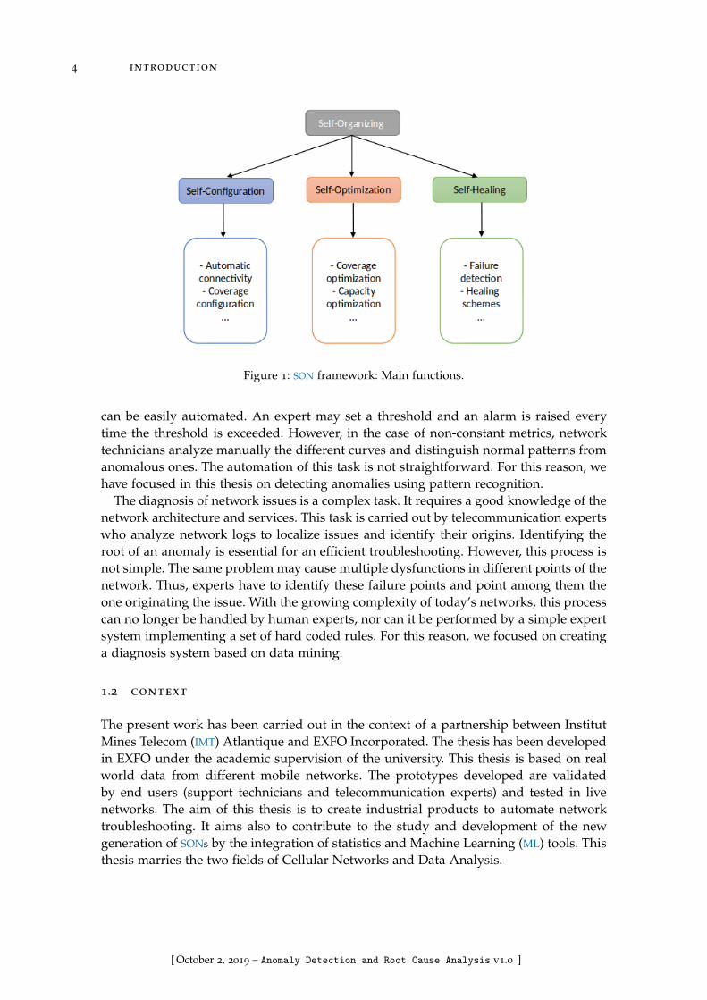
To provide various services with high Quality of Service (QoS), researchers in the areaof cellular networks introduced new paradigms to ease the management tasks and theimplementation of new functionalities. One of the key concepts introduced in LTE and 5Gis the concept of Self-Organizing Networks (SONs) [38], [64]. The idea of self-organizationrefers to the automation of the processes that are usually conducted by experts andtechnicians. We identify three main functionalities related to SONs: self-configuration,self-optimization, and self-healing. Figure 1 illustrates this analysis. Self-configurationaims at the automation of the installation procedures. For instance, a new deployedEvolved Node B (eNodeB) can be automatically configured based on its embedded soft-ware and the data downloaded from the network without any human intervention. Self-optimization is the process of the automatic tuning of the network based on performancemeasurements. Self-healing refers to detecting network issues and solving them in anautomatic and dynamic manner. In this thesis, we focus on this latter aspect. We conducta study of self-healing techniques and propose a potential solution [98], [99].
The healing process is made up of four main tasks [75]. It starts with the detection ofan issue in the network such as the degradation of a Key Performance Indicator (KPI).Once a problem is detected, one should carry out an in-depth analysis to diagnose theproblem and find its root causes. Depending on the nature of the problem, two cases arepossible. If the problem can be solved within a short time (few minutes), the recoveryprocess is triggered and there is no need for compensation. On the contrary, if the re-covery process is slow, compensation measures are taken to guarantee the availability ofthe network during the recovery process. The compensation and the recovery processesdepend on the accuracy of the detection and the diagnosis. The main topic of this thesisis related to the two first phases of the healing process: the detection and the diagnosis.We aim to create an autonomous system that detects anomalies in real time and iden-tifies their root causes in order to help experts to decide about the adequate recoveryactions.
The detection of network issues is a part of the daily tasks of network technicians andadministrators. To identify issues they check network metrics and KPIs to make sure theirvalues are within the normal range. Detecting anomalies on metrics with constant values
3
[ October 2, 2019 – Anomaly Detection and Root Cause Analysis v1.0 ]
4 introduction
Figure 1: SON framework: Main functions.
can be easily automated. An expert may set a threshold and an alarm is raised everytime the threshold is exceeded. However, in the case of non-constant metrics, networktechnicians analyze manually the different curves and distinguish normal patterns fromanomalous ones. The automation of this task is not straightforward. For this reason, wehave focused in this thesis on detecting anomalies using pattern recognition.
The diagnosis of network issues is a complex task. It requires a good knowledge of thenetwork architecture and services. This task is carried out by telecommunication expertswho analyze network logs to localize issues and identify their origins. Identifying theroot of an anomaly is essential for an efficient troubleshooting. However, this process isnot simple. The same problem may cause multiple dysfunctions in different points of thenetwork. Thus, experts have to identify these failure points and point among them theone originating the issue. With the growing complexity of today’s networks, this processcan no longer be handled by human experts, nor can it be performed by a simple expertsystem implementing a set of hard coded rules. For this reason, we focused on creatinga diagnosis system based on data mining.
1.2 context
The present work has been carried out in the context of a partnership between InstitutMines Telecom (IMT) Atlantique and EXFO Incorporated. The thesis has been developedin EXFO under the academic supervision of the university. This thesis is based on realworld data from different mobile networks. The prototypes developed are validatedby end users (support technicians and telecommunication experts) and tested in livenetworks. The aim of this thesis is to create industrial products to automate networktroubleshooting. It aims also to contribute to the study and development of the newgeneration of SONs by the integration of statistics and Machine Learning (ML) tools. Thisthesis marries the two fields of Cellular Networks and Data Analysis.
[ October 2, 2019 – Anomaly Detection and Root Cause Analysis v1.0 ]
1.3 objectives 5
1.3 objectives
Our goal is to study and propose techniques to design self-healing networks. The pro-posed techniques are based on data analysis concepts. In other terms, we work on al-gorithms allowing the extraction of information relevant to the troubleshooting processfrom the large amount of data produced by the cellular network. As stated earlier, wefocus here on the detection and diagnosis tasks of the self-healing process. So this thesishas two major objectives:
• Anomaly detection: Our goal is to detect anomalies in the network in real time. Thedetection should be automatic and unsupervised. The proposed solution shouldlearn from previous data without including any expert rules. It should also bedynamic and capable to adapt to the network evolution. Furthermore, the pro-posed solution should be efficient (having low error rate with few computationalresources). In practical terms, the solution should be implemented as a module ofa monitoring system and has to process the metrics it creates. To detect networkissues, the solution should detect the anomalous patterns in the curves represent-ing the network metrics. Once an anomaly is detected, an alarm is raised to notifythe network administrator about the details of the issue.
• Root cause diagnosis: Our objective is to create a solution that analyses the Endto End (E2E) cellular network and find the roots of the issues within the network.This solution should be unsupervised and automatic. It has to identify major high-impact causes at the first place. Localizing less important causes with lower impactis also part of the study. The solution should function without any prior knowledgeof the network topology and its computational complexity should be reasonable.The solution for root cause diagnosis should be part of the monitoring system.It should be connected to the anomaly detection module. Once an anomaly isdetected, the diagnosis could be automatically triggered. The result of the analysisshould contain all the information needed for the troubleshooting process. Theinformation should be presented in a way that is easily understandable by theexperts.
For each of the two objectives, we aim to create a prototype and validate it in both alab environment and a real network. Once the solution is validated, we aim to transformit into an industrial product that will go to the market as part of EXFO solutions.
1.4 challenges
Creating an automatic solution for network anomaly detection is challenging in two ma-jor aspects: data handling and integration within the monitoring system. The first aspectis related to data preparation and processing. The metrics of the monitoring system canbe either constant, periodic, or chaotic. As our objective here is to address the issue ofanomaly detection in periodic data, the solution has to automatically identify the typesof the metrics and process only periodic ones. Periodicity detection is not easy, especiallyin irregular metrics where the interval between different samples is not constant. This isalways the case in real monitoring systems where the data measurements are controlled
[ October 2, 2019 – Anomaly Detection and Root Cause Analysis v1.0 ]

6 introduction
by queuing systems. Moreover, the solution has to learn a short history of data as mon-itoring systems are designed to erase data regularly. The solution has also to adapt tothe natural growth of the traffic. This growth should be integrated into the model ofdata created by the solution in order to prevent it from being detected as an anomaly.Another challenging fact is the various patterns of anomalies. The solution has to detectnew anomaly patterns that were not predefined during the implementation. The secondaspect concerns the integration of the solution in the monitoring system. The solutionshould be transparent and not interfere with any other monitoring process. Thus, it hasto have few computational and memory needs. The solution should not require any postimplementation effort from experts. Consequently, all the detection steps should be fullyautomatic. Finally, the solution has to provide accurate results which is not easy withfew calculation resources.
The diagnosis task demands a deep analysis of the data logs to identify the root causeof issues. Automating this process is challenging as it requires both domain knowledgeand analysis capabilities from experts. The network architecture is needed to diagnosenetwork issues. However defining it manually requires a large effort prior to the in-stallation of the solution. Added to that, this information has to be updated each timethe architecture is modified. To overcome this difficulty, the architecture can be dis-covered automatically based on the data. However, the inference of such complicatedstructure may require a lot of calculations. The network architecture is not the onlyinformation needed for the analysis. The structure of services provided by Internet Ser-vice Providers (ISPs) and web content providers is also required. Besides, the analysisof communication logs to extract information about issues is challenging in multipleaspects. The number of communication logs is huge, each having a large number offeatures. The features may be related. There is no dependency chart defining explicitlythe relations between different features. Another challenging point is the large varietyof network issues. Some issues may be interrelated and thus more complicated to bediagnosed automatically. The network issues do not have the same importance and thusa prioritization task must be included within the diagnosis process.
1.5 contribution
This thesis contributes to the research and industry in the field of network monitoring.As stated, we address here two major questions related to the concept of self-healingnetworks. The first subject is the detection of anomalies in network metrics. In thisthesis, we propose a fully unsupervised solution, Watchmen Anomaly Detection (WAD)to this question. This solution has been industrialized and added to two monitoringtools to alleviate the load of network administrators. The second question is diagnosisof the root causes of network issues. Our solution, Automatic Root Cause Diagnosis(ARCD) is unsupervised and implements a large part of telecommunication experts tasks.ARCD analyses communication logs and creates an overview of issues at multiple levels.This fact reduces the expert role to validating the output of ARCD before triggering theadequate healing scheme. The industrialization of ARCD is ongoing and the first resultsare promising.
[ October 2, 2019 – Anomaly Detection and Root Cause Analysis v1.0 ]

1.6 document structure 7
1.6 document structure
This document is composed of three parts. The first part is an introductory part. It con-tains the introduction, a chapter about the telecommunication background and anotherone on the data analysis background. In the telecommunication background, we give anoverview of cellular networks and monitoring systems. In the data analysis chapter, weintroduce time series and multidimensional analysis as one needs some basic notionsin these topics to understand the remainder of the thesis. The second part is about thefirst objective of the thesis: anomaly detection. In this part, we start by a study of thestate of the art. Then, we present the theoretical and practical results of the solution wepropose. We finish by a brief description of the industrialization process of our solution.The third part is about the second objective of the thesis: root cause diagnosis. As for theprevious objective, we review the state of the art, introduce our solution and describethe industrialization process. In the conclusion, we recall the main results and give somepotential future works.
[ October 2, 2019 – Anomaly Detection and Root Cause Analysis v1.0 ]

[ October 2, 2019 – Anomaly Detection and Root Cause Analysis v1.0 ]
2T E L E C O M M U N I C AT I O N B A C K G R O U N D
In this chapter, we introduce some telecommunication concepts relevant to the remain-der of the thesis. As stated in the objective of the thesis, our aim is to create an anomalydetection and root cause diagnosis solution in cellular networks. We start by giving anoverview of today’s cellular networks architecture and services. Then, we highlight theircomplexity and list their requirements in terms of performance and reliability. There-after, we give a short overview of the state of the art of monitoring systems and we detailsome of their functions. We finish by highlighting the gap between the required capa-bilities of monitoring systems and their current performance. Our work is an attemptto close this gap by proposing algorithms filling two important monitoring functions:anomaly detection and root cause diagnosis.
2.1 cellular networks
Mobile operators offer different types of services ranging from basic services such as con-versational voice, Short Messaging Service (SMS), Multimedia Messaging Service (MMS),and Unstructured Supplementary Service Data (USSD) to more complex ones appearingwith the emergence of smart phones such as real time gaming, video chatting, videostreaming and other web based services like browsing, email, social networking, andPeer to Peer (P2P) file transfer. With the arrival of 5G, more services are expected to ap-pear based on Internet of Things (IoT) and Machine to Machine (M2M) related to smartcities and smart homes [9], [35]. The multitude and heterogeneity of services make thenetwork infrastructure more and more complex. In this section, we give a brief overviewof cellular networks architecture. Then, we explain briefly the complexity of networkmanagement and list cellular network requirements with regard to Third GenerationPartnership Project (3GPP) standards.
2.1.1 Architecture
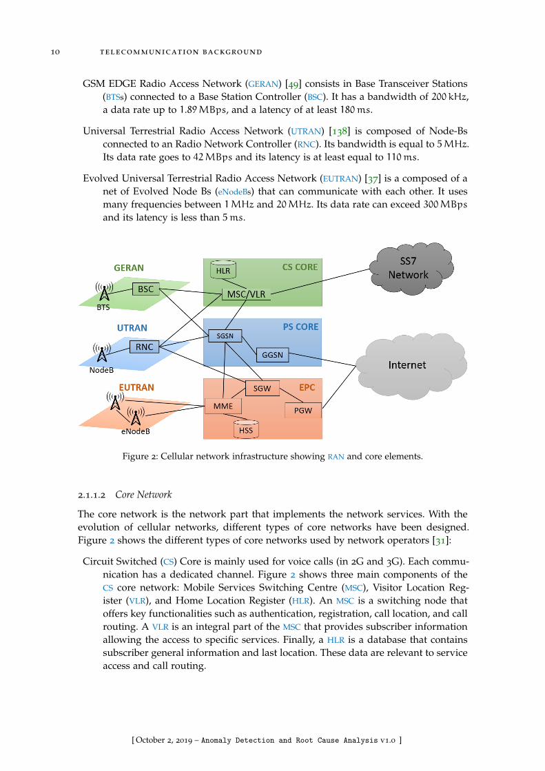
To reduce costs and ease the transition from one generation to another, 2G, 3G and4G coexist in today’s cellular network infrastructure. We will give now a brief view ofthe different technologies present in the Radio Access Network (RAN) and in the corenetwork.
2.1.1.1 RAN
The RAN is the wireless part of the network that connects subscriber devices to the corenetwork. It implements one or multiple Radio Access Technologies (RATs). As illustratedin Figure 2, in today’s RAN we find the following RATs:
9
[ October 2, 2019 – Anomaly Detection and Root Cause Analysis v1.0 ]
10 telecommunication background
GSM EDGE Radio Access Network (GERAN) [49] consists in Base Transceiver Stations(BTSs) connected to a Base Station Controller (BSC). It has a bandwidth of 200 kHz,a data rate up to 1.89MBps, and a latency of at least 180ms.
Universal Terrestrial Radio Access Network (UTRAN) [138] is composed of Node-Bsconnected to an Radio Network Controller (RNC). Its bandwidth is equal to 5MHz.Its data rate goes to 42MBps and its latency is at least equal to 110ms.
Evolved Universal Terrestrial Radio Access Network (EUTRAN) [37] is a composed of anet of Evolved Node Bs (eNodeBs) that can communicate with each other. It usesmany frequencies between 1MHz and 20MHz. Its data rate can exceed 300MBpsand its latency is less than 5ms.
Figure 2: Cellular network infrastructure showing RAN and core elements.
2.1.1.2 Core Network
The core network is the network part that implements the network services. With theevolution of cellular networks, different types of core networks have been designed.Figure 2 shows the different types of core networks used by network operators [31]:
Circuit Switched (CS) Core is mainly used for voice calls (in 2G and 3G). Each commu-nication has a dedicated channel. Figure 2 shows three main components of theCS core network: Mobile Services Switching Centre (MSC), Visitor Location Reg-ister (VLR), and Home Location Register (HLR). An MSC is a switching node thatoffers key functionalities such as authentication, registration, call location, and callrouting. A VLR is an integral part of the MSC that provides subscriber informationallowing the access to specific services. Finally, a HLR is a database that containssubscriber general information and last location. These data are relevant to serviceaccess and call routing.
[ October 2, 2019 – Anomaly Detection and Root Cause Analysis v1.0 ]
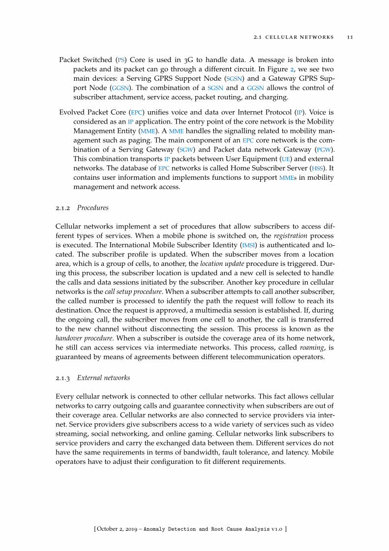
2.1 cellular networks 11
Packet Switched (PS) Core is used in 3G to handle data. A message is broken intopackets and its packet can go through a different circuit. In Figure 2, we see twomain devices: a Serving GPRS Support Node (SGSN) and a Gateway GPRS Sup-port Node (GGSN). The combination of a SGSN and a GGSN allows the control ofsubscriber attachment, service access, packet routing, and charging.
Evolved Packet Core (EPC) unifies voice and data over Internet Protocol (IP). Voice isconsidered as an IP application. The entry point of the core network is the MobilityManagement Entity (MME). A MME handles the signalling related to mobility man-agement such as paging. The main component of an EPC core network is the com-bination of a Serving Gateway (SGW) and Packet data network Gateway (PGW).This combination transports IP packets between User Equipment (UE) and externalnetworks. The database of EPC networks is called Home Subscriber Server (HSS). Itcontains user information and implements functions to support MMEs in mobilitymanagement and network access.
2.1.2 Procedures
Cellular networks implement a set of procedures that allow subscribers to access dif-ferent types of services. When a mobile phone is switched on, the registration processis executed. The International Mobile Subscriber Identity (IMSI) is authenticated and lo-cated. The subscriber profile is updated. When the subscriber moves from a locationarea, which is a group of cells, to another, the location update procedure is triggered. Dur-ing this process, the subscriber location is updated and a new cell is selected to handlethe calls and data sessions initiated by the subscriber. Another key procedure in cellularnetworks is the call setup procedure. When a subscriber attempts to call another subscriber,the called number is processed to identify the path the request will follow to reach itsdestination. Once the request is approved, a multimedia session is established. If, duringthe ongoing call, the subscriber moves from one cell to another, the call is transferredto the new channel without disconnecting the session. This process is known as thehandover procedure. When a subscriber is outside the coverage area of its home network,he still can access services via intermediate networks. This process, called roaming, isguaranteed by means of agreements between different telecommunication operators.
2.1.3 External networks
Every cellular network is connected to other cellular networks. This fact allows cellularnetworks to carry outgoing calls and guarantee connectivity when subscribers are out oftheir coverage area. Cellular networks are also connected to service providers via inter-net. Service providers give subscribers access to a wide variety of services such as videostreaming, social networking, and online gaming. Cellular networks link subscribers toservice providers and carry the exchanged data between them. Different services do nothave the same requirements in terms of bandwidth, fault tolerance, and latency. Mobileoperators have to adjust their configuration to fit different requirements.
[ October 2, 2019 – Anomaly Detection and Root Cause Analysis v1.0 ]
12 telecommunication background
2.1.4 Cellular network requirements
The telecommunication market standards define challenging criteria that should befilled [3], [45]. First, high performance is the most important targeted criterion. Opera-tors aim to deliver an elevated Quality of Service (QoS) and Quality of Experience (QoE).They have to assure high responsiveness by reducing the latency and increasing thethroughput. They also have to ensure high connectivity by densifying their networkand widening their coverage areas (indoor/outdoor). Second, operators work towardshaving a resilient and flexible network with an adaptive capacity to support disruptive aswell as natural traffic growth. Third, operators aim to have a fault tolerant network thatguarantees a constant availability of the services by implementing compensation andfast recovery mechanisms. Lastly, standards value security and privacy. Operators shouldsecure their networks from attacks against both integrity and privacy.
2.2 monitoring systems
As shown in the previous section, cellular networks are very complex to monitor. Atthe same time, the telecommunication market and the standardization entities pushoperators to deliver high quality services. These facts make the monitoring systems acritical component of today’s cellular networks. Many operators outsource a part of theirmonitoring tasks to specialized companies such as EXFO.
The goal of monitoring the cellular network is to have full visibility and control overthe network infrastructure and processes. This task is carried out by experts in differ-ent domains: network administrators, software technicians, Information Technology (IT)specialists, and telecommunication experts. The goal of integrating monitoring systemsis to increase the speed and efficiency of these experts by automating tasks and provid-ing useful information. In the following, we detail the main functions of a monitoringsystem.
2.2.1 Main functions
The monitoring functions can be grouped into three categories: troubleshooting, perfor-mance monitoring, and planning. Some operators use a centralized monitoring systemthat incorporates the three categories. Others use multiple systems, each implementinga subset of the monitoring functions. We detail now each category of functions.
Troubleshooting is the most important monitoring function as operators want theirservices to be continuously available. The troubleshooting process can be brokendown into four main functions [124]: data collection, issue detection, issue identi-fication, and recovery. Data collection consists in collecting data that is relevant tothe troubleshooting process by creating and/or collecting logs, recording events,mirroring the traffic, generating reports, and calculating metrics. The second step,issue detection, consists in analyzing logs and evaluating metrics to detect anoma-lies. If an abnormal event is found in the logs or a metric has an abnormal value,the operator is notified. The notification can take different forms such as raisingan alarm or creating a ticket. The third function, issue identification consists in
[ October 2, 2019 – Anomaly Detection and Root Cause Analysis v1.0 ]

2.2 monitoring systems 13
a deep analysis of the data to diagnose the network and identify the issue. Fi-nally, the recovery step consists in fixing the problem by triggering the adequatecompensation and recovery mechanisms. The mentioned functions can be manual,partially automated, or fully automated.
Performance monitoring consists in measuring Key Performance Indicators (KPIs) togain insights on network performance, benchmark network elements (e.g. cells)and services, and identify the low performing ones. Through performance moni-toring, operators may improve the QoS and therefore the QoE [88].
Prediction and planning are based on process/resource monitoring. By analyzing KPI
trends, operators can improve their services in different ways. As an example,they can anticipate events and prevent downtime [54]. Furthermore, they can pre-dict churn and propose more personalized subscriptions [125]. Moreover, they canallocate resources more efficiently [60].
2.2.2 Structure
Monitoring systems have different structures depending on many factors such as the sizeof the network, the load of the traffic, the main afforded services, and the preferences ofthe operator. The monitoring system can be centralized or distributed. In the following,we focus on the four main components that are present in almost every monitoringsystem.
Probes [83], [136] are mirroring components that can be built in the network monitor-ing tool or installed separately in the monitored devices. Probes pull data fromdevices passively in real time using protocols like Simple Network ManagementProtocol (SNMP), Transmission Control Protocol (TCP), and Hypertext Transfer Pro-tocol (HTTP).
A data processing entity is considered as the brain of the monitoring system. It imple-ments basic functionalities such as data filtering and aggregation. It also includesadvanced functionalities such as trend analysis, anomaly detection, network diag-nosis, capacity planning, and QoE estimation based on Business Intelligence (BI)and Machine Learning (ML) tools. This component creates KPIs, generates statusinformation, and summary reports.
An alerting system triggers real time alarms based on the information offered by thedata processing entity. For example, it notifies the administrators if a KPI is belowa predefined threshold.
A visualization system is a Graphical User Interface (GUI) that displays the summaryinformation in a human readable manner. It enables the administrator to navigatethe different components of the network and to visualize status and performancestatistics.
[ October 2, 2019 – Anomaly Detection and Root Cause Analysis v1.0 ]
14 telecommunication background
2.2.3 Data types
The monitoring systems produce two types of logs: communication logs and systemlogs [137]. Communication logs are the logs a monitoring system keeps from subscribersactivity such as call traces. Call traces are unstructured data including all the messagesexchanged by network devices during a mobile communication initialized by a sub-scriber. These traces are aggregated into Call Data Records (CDRs) and Session DataRecords (SDRs) which are structured logs containing the list of the network devices andthe service details involved in the mobile communication. CDRs are the records of voicecalls and SDRs are the records of TCP connections. CDRs and SDRs are aggregated intomultidimensional counters reporting the performance of the network (e.g. the mean re-sponse time by the 3-tuple (RAT, service, handset type)). System logs are the logs createdto keep track of the events, processes and messages of the system such as Address Res-olution Protocol (ARP) requests. Alerts are created based on these logs (whenever anabnormal event occurs). System logs and communication logs are aggregated into KPIs
which are time series presenting the temporal evolution of performance indicators suchas the Central Processing Unit (CPU) usage and the call drop rate.
2.2.4 Requirements
To guarantee network high performance, the monitoring system has to be effective. Theeffectiveness translates in terms of different requirements. First, the monitoring sys-tem should scale to handle the growth of the traffic and the expansion of cellular net-works [85]. Second, the monitoring system should be flexible to supervise multi-vendorand heterogeneous network equipments [69]. Third, the monitoring system should besufficiently reactive to detect issues and trigger mitigation operations in real time to limitdowntime. In addition, it should perform an in-depth analysis of the network and goto fine granularity levels to find hidden issues. Fourth, the monitoring system shouldbe autonomous to a certain degree to be reactive and reduce demanded human efforts.Repetitive tasks should be automated. More advanced tasks can be partially automatedby the use of ML [88], [124]. The settings of the monitoring system should be straight-forward [88]. Moreover, it has to be compliant with telecommunication standards and market.The monitoring system should respect the standards by insuring the demanded QoS. Ithas also to respond to the marked needs [2], [4], [87] (e.g. integrating new functions tomonitor new services). Furthermore, it should be fault tolerant and easy to troubleshoot.Lastly, the monitoring system has to be cost-effective. As the network traffic is huge, theanalysis implemented in the monitoring system should be optimized to reduce compu-tational needs. The monitoring system should also store only needed data and for alimited period of time.
2.2.5 Limitations
While the monitoring systems have evolved in terms of autonomy and efficiency, theyare still below the requirements mentioned in the previous paragraph in many aspects:First, the monitoring process still relies on the human presence. Many monitoring tasks
[ October 2, 2019 – Anomaly Detection and Root Cause Analysis v1.0 ]

2.2 monitoring systems 15
today are carried out manually. While monitoring systems generate KPIs and alarms,these latter are analyzed by experts when troubleshooting the network. This fact makesthe troubleshooting task very costly to operators. Second, the cellular networks still suf-fer from low efficiency occasionally (downtime) or continually in some specific casessuch as roaming and mobility. The monitoring systems are not sufficiently reactive andefficient to address unavailable services in real time nor to handle roaming and han-dovers in an optimal way. Last, the 5G standards have set high expectations in termsof QoS. The current monitoring systems are not capable of guaranteeing such perfor-mance [127].
[ October 2, 2019 – Anomaly Detection and Root Cause Analysis v1.0 ]

[ October 2, 2019 – Anomaly Detection and Root Cause Analysis v1.0 ]

3D ATA A N A LY S I S B A C K G R O U N D
In this chapter, we go through the data analysis background needed for the thesis. Westart by giving an overview of time series which is the main mathematical concept weneed to go through Part ii. Then, we will briefly introduce multidimensional analysiswhich is the mathematical basis of Part iii.
3.1 time series
3.1.1 Definitions
An univariate time series x(t) is a sequence of measurements of a single variable thatis time dependent [19]. It is often denoted X(t) = x(t)|t ∈ T where T is the time index.Figure 3 is an example of time series. It shows the evolution of the number of call logs inan interface between two monitoring devices: a Neptune™probe and a hub over time.
A multivariate time series, as its name suggests, is a sequence of measurements ofmultiple variables. The variables are co-dependent and depend also on time.
In the following, we denote the average and the standard deviation of a time seriesx(t) as:
µx(t) = E[x(t)] (1)
σx(t) =√E[(x(t) − µx(t))2] (2)
where the operator E[x] denotes the expectation of x.x(t) is said to be (weakly) stationary if µx and σx are not time dependent. This as-
sumption is crucial in many time series models.
3.1.2 Seasonal time series
A seasonal or periodic time series is a series that verifies x(t+m) = x(t) where m iscalled the period of the series. Seasonal time series exhibits a repetitive pattern at regulartime intervals. This seasonality comes from many factors depending on the domain. Forexample, in cellular networks, the seasonality is explained by the repetitive behaviourand the lifestyle of subscribers: few calls during the night, a peak in calls at 12 am and6 pm as shown in Figure 3.
Seasonal times can be decomposed into three components:
• The trend which is the long term variations of the series. It can be deduced usingfiltering or polynomial fitting techniques.
• The seasonal component which contains the repetitive pattern. It can be deducedfrom a harmonic analysis.
• The residual component which contains the random variation in the time series.
17
[ October 2, 2019 – Anomaly Detection and Root Cause Analysis v1.0 ]

18 data analysis background
Figure 3: An example of time series:The number of CDRs in an interface of a monitoring probe over time.
Figure 4 shows a time series of the number of CDR in a probe interface. The timeseries is decomposed into its trend, seasonal and residual components. The trend showsthat the traffic is increasing over time. The seasonal component shows a perfect dailyperiodicity in the number of calls. The residual component contains noise effects andabrupt changes in the traffic.
Figure 4: The decomposition of a time series into its trend, seasonal and residual components.
3.1.3 Time analysis
This type of analysis consists on analyzing the series in the time domain. One of the mostknown techniques is the Autocorrelation Function (ACF). It helps in identifying patternsand finding periodicity. The ACF analysis is a base of the auto-regressive models used in
[ October 2, 2019 – Anomaly Detection and Root Cause Analysis v1.0 ]
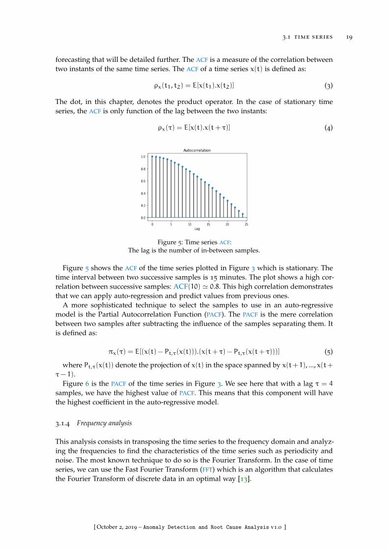
3.1 time series 19
forecasting that will be detailed further. The ACF is a measure of the correlation betweentwo instants of the same time series. The ACF of a time series x(t) is defined as:
ρx(t1, t2) = E[x(t1).x(t2)] (3)
The dot, in this chapter, denotes the product operator. In the case of stationary timeseries, the ACF is only function of the lag between the two instants:
ρx(τ) = E[x(t).x(t+ τ)] (4)
Figure 5: Time series ACF:The lag is the number of in-between samples.
Figure 5 shows the ACF of the time series plotted in Figure 3 which is stationary. Thetime interval between two successive samples is 15 minutes. The plot shows a high cor-relation between successive samples: ACF(10) ' 0.8. This high correlation demonstratesthat we can apply auto-regression and predict values from previous ones.
A more sophisticated technique to select the samples to use in an auto-regressivemodel is the Partial Autocorrelation Function (PACF). The PACF is the mere correlationbetween two samples after subtracting the influence of the samples separating them. Itis defined as:
πx(τ) = E[(x(t) − Pt,τ(x(t))).(x(t+ τ) − Pt,τ(x(t+ τ)))] (5)
where Pt,τ(x(t)) denote the projection of x(t) in the space spanned by x(t+ 1), ..., x(t+τ− 1).
Figure 6 is the PACF of the time series in Figure 3. We see here that with a lag τ = 4
samples, we have the highest value of PACF. This means that this component will havethe highest coefficient in the auto-regressive model.
3.1.4 Frequency analysis
This analysis consists in transposing the time series to the frequency domain and analyz-ing the frequencies to find the characteristics of the time series such as periodicity andnoise. The most known technique to do so is the Fourier Transform. In the case of timeseries, we can use the Fast Fourier Transform (FFT) which is an algorithm that calculatesthe Fourier Transform of discrete data in an optimal way [13].
[ October 2, 2019 – Anomaly Detection and Root Cause Analysis v1.0 ]

20 data analysis background
Figure 6: Time series PACF:The lag is the number of in-between samples.
Figure 7: Time series FFT.The two important symmetrical components correspond to daily periodicity.
[ October 2, 2019 – Anomaly Detection and Root Cause Analysis v1.0 ]

3.1 time series 21
Figure 7 is the FFT of the time series in Figure 3. The central component at freq=0
corresponds to the mean of the time series. The two high symmetrical components cor-respond to the daily seasonality of the time series. The plot shows also some otherperiodical variations. These is no high frequencies with important amplitudes, whichmeans that the noise in the time series is not significant. Other techniques to study timeseries in the frequency domain exists such as the Wavelet Transform. The details arein [5].
3.1.5 Forecasting in time Series
Time series are used in many areas to do forecasting. Forecasting is important notonly for planning and optimization but also in predicting issues in order to preventthem or limit their extent. The most widely used model for time series forecasting isAutoregressive Moving Average (ARMA), [19]. ARMA is the combination of two modelsapplicable to stationary time series: an Autoregressive (AR) model and a Moving Aver-age (MA) model. In the case of non stationarity, the time series is differentiated multipletimes until stationarity. Then the model is applied (Autoregressive Integrated MovingAverage (ARIMA)).
An AR model of order p, AR(p) is denoted as:
x(t) = c+
p∑i=1
ψi.x(t− i) + ε(t) (6)
where c is a constant, ψ1, ...,ψp are regression parameters and ε(t) is a variable thatmodels the noise of the time series. Equation (6) shows that AR models can handleseasonality if samples from previous periods are included in the model x(t− T).
A MA model of order q, MA(q) is denoted as:
x(t) = µ+ ε(t) +
q∑i=1
θi.ε(t− i) (7)
where µ is the expectation of x(t), θ1, ..., θq are the parameters of the model and ε(t)is a variable that models the noise. As in Equation (7), MA models are flexible as theyestimate the current value of a time series based on previous values of the noise variable.
An ARMA model of orders p and q, ARMA(p,q) is denoted as:
x(t) = c+
p∑i=1
ψi.x(t− i) + ε(t) +q∑i=1
θi.ε(t− i) (8)
The ARMA models are widely used thanks to their flexibility and precision. The coeffi-cients of the model are fitted using the least squares regression. The selection of p and qis generally based on the PACF and the ACF. The selection can be also made on the basisof Akaike Information Criterion (AIC) [15].
[ October 2, 2019 – Anomaly Detection and Root Cause Analysis v1.0 ]

22 data analysis background
3.1.6 Patterns in time series
Time series can display specific patterns that would be relevant to the use case of theanalysis. The idea of pattern recognition in time series is not new and has been ap-proached in different ways. The time series is split into segments [71] and the segmentscould be classified into classes of patterns [61]. The classification can be based on anyMachine Learning (ML) algorithm such as K-means, neural networks, Support VectorMachine (SVM), decision trees, etc. Seasonal time series, because of their periodicity, aregood candidates to be analyzed via pattern recognition tools.
3.2 multidimensional analysis
Multidimensional analysis presents many challenges. In the following, we give a brieftour of its main concepts.
3.2.1 Numerical vs categorial data
In a data set, the features may have different types: numerical, categorial [7] or mixed.In the case of numerical data, a large panel of analysis tools is available. The data canbe processed in different ways by applying mathematical functions. The precision of theanalysis can be measured and the error can be quantified. The visualization of data issimple and the distance between the samples is calculated in an intuitive way. However,for categorial data, the features are rather qualitative and we have less analysis tools.Values are not always comparable. The concept of distance depends on the use case andcannot be generalized, although some distance measures exist such as the Hammingdistance. The error and precision are context dependent.
In both cases, we have specific tools to deal with each type of data. The challengeis when we have mixed data (numerical and categorial features). In this case, very fewalgorithms are applicable. To overcome this barrier, two solutions are possible: either wetranspose numerical data into categorial data by discretization or we transform categor-ical data into numerical by encoding it. Discretization consists in mapping numericalvalues into qualitative levels by setting thresholds. For example, in the case of responsetime in Transmission Control Protocol (TCP) connections, we may consider a responsetime below 20ms as good, between 20ms and 100ms as acceptable and a response timehigher than 100ms as bad. Discretization is practical, however it induces an obvious lossof information. Encoding is the process of converting categorial values to numerical val-ues. Many encoders have been proposed [117]. We cite here, the ordinal and the OneHotencoders. The ordinal encoder converts a categorial feature with k different values to in-tegers from 1 to k. By the means of this encoder, we are capable of applying regressiontechniques to categorial data. However, the notions of distance and proportionality areirrelevant and the results are very likely to be biased. In the case of OneHot encoder,for each value of a categorial feature, we create a binary column. So a categorial featurewith k different values is replaced with k numerical (binary) features. This encoder maydrastically increase the dimensionality of data and therefore the execution time of theanalysis.
[ October 2, 2019 – Anomaly Detection and Root Cause Analysis v1.0 ]
3.2 multidimensional analysis 23
3.2.2 Sampling
In some cases of high volumes of data (Big Data), it is not advised to process the wholedata for both cost and practicality reasons. In these cases, sampling is a necessity ratherthan an option. Sampling [27] is defined as the selection of a subset of samples froma data set on which the analysis will be performed. By using sampling, the processingtime is reduced and the application of complex models is possible. There are many pos-sible approaches to perform sampling such as random selection, cluster sampling, andstratified sampling. The selection of the sample size is not straightforward. It dependson many factors such as the analysis techniques that will be applied, the available com-putational resources, and the required accuracy of the results. As the selected subsetis not perfectly representative of the original set, many types of errors are induced. Afirst type of errors is sample over-fitting. In this case, the inferred model fits perfectlythe sample. However, it does not fit the original data set. In our context of designingmonitoring systems for mobile operators, one may think of a solution perfectly fitting aspecific network but giving random results for other networks. Another type of errorsis the random sampling error, where the results display random variations originatedfrom the random selection in the sampling process. This can be the case of a tendencyartificially created by a random selection of points.
3.2.3 Dimensionality reduction
During the data collection process, administrators in the telecommunication domaintend to log every bit of information that could be useful for analysis. Today, we are ableto have an End to End (E2E) view of communications including details about the involveddevices, service information, and protocol messages. While being comprehensive, thedata analysis task becomes cumbersome. Analyzing data with a high number of featuresrequires both large computation resources and huge human efforts. That is why it isnecessary to reduce data dimensionality.
Dimensionality reduction is beneficial with regard to many aspects. First, it is costeffective: It reduces the computation time and resources. It also reduces the storageresources by compressing high dimensional data into low dimensional data and remov-ing redundant features. Second, it allows us to have simple data models that are easilyunderstood and interpreted. It also eases data visualization. Last, it allows us to ap-ply complex algorithms. Some algorithms perform very poorly when applied to highdimensional data compared to low dimensional data. This fact is known as the curseof dimensionality. By reducing the number of features, it is possible to remove noisefeatures and have more accurate results. To perform dimensionality reduction, two ap-proaches are possible [72]:
feature selection consists in the selection of a subset of features that are relevant tothe analysis. Multiple techniques exist depending in the model input (numerical orcategorial data) and the output of the analysis (classification or regression). Table 1
gives some examples of the used techniques.
feature extraction consists in combining multiple features in order to transforma high dimensional analysis space to a low dimensional analysis space. The most
[ October 2, 2019 – Anomaly Detection and Root Cause Analysis v1.0 ]

24 data analysis background
Input
OutputNumerical (Regression) Categorial (Classification)
Numerical Pearson correlation: measuresthe linear correlation betweenthe input and the output vari-able of the regression.
LDA: identifies a linear combi-nation of variables that sepa-rates the different classes of acategorial variable.
Categorial T-test/ANOVA: test if the meanof the output is the same ineach class of the input.
χ2-test: quantifies the correla-tion between two categorialvariables based on their distri-butions.
Table 1: Feature selection techniques by input/output type.
known technique is Principal Component Analysis (PCA). PCA creates a linear com-bination of numerical inputs that maximizes the variance. The concept behind PCA
is that variables with low variance (almost constant) are not useful in the datamodel. Feature extraction can also be performed using ML algorithms such as neu-ral networks and decision trees.
3.2.4 Statistical Inference
Statistical inference aims at creating a model that highlights specific characteristics ofdata [22]. The model could be for example the distribution of a random variable. Themodel selection can be subjective based on intuition or expertise in the domain or ob-jective based on statistical tests such normality tests. Models can be parametric or nonparametric. Most of the used models are parametric and the estimation of parametersis the core of data analysis process. To this aim, many estimators have been proposedsuch as Bayesian estimator and Maximum likelihood. Some estimators return an intervalrather than a value of the parameter with a confidence coefficient of the real parameterto be in that interval.
Hypothesis testing has been introduced to validate models or assumptions in general.Hypothesis testing is a formal procedure to accept or reject an assumption (e.g. a modelparameter value). It consists on formulating a null hypothesis (the proposed model) andan alternative hypothesis. The second step is then to identify a test statistical to evaluatethe truth of the null hypothesis. Depending on the type of the hypothesis many testshave been defined such as χ2-tests, t-tests, z-test, etc. These tests allow to accept orreject the null hypothesis with a confidence parameter (p-value). If the null hypothesisis rejected, the alternative hypothesis is considered to be true.
3.2.5 Machine Learning
Machine Learning (ML) [142] is an area of data analysis, where the algorithm learnscontinuously from data and improves its precision. ML aims at imitating human learning,reasoning and decision making. Unlike expert systems which are automated systems
[ October 2, 2019 – Anomaly Detection and Root Cause Analysis v1.0 ]

3.2 multidimensional analysis 25
based on human expertise, ML-based systems rely completely on the system to learnfrom data. The intelligence of ML algorithms comes from the iterative processing of datauntil convergence or attaining a high precision. ML allows to build autonomous systemswith an embedded artificial intelligence. There are two phases in an ML algorithm: atraining phase where the system learns from data and a test phase when the algorithmapplies the acquired knowledge to new samples. The system keeps learning from newdata to increase its performance.
There are two types of ML algorithms: supervised and unsupervised. Supervised ML iswhen the expected outcome of the algorithm is known for the data used in the trainingphase. In this case, the algorithm can be finely tuned to have a high precision. In thecase of unsupervised learning, the expected outcome of the training data is unknown.In most of the real world cases, we have to work with unsupervised ML as manuallyspecifying the expected outcome for training data can be either difficult or very timeconsuming. However, we can specify the expected outcome for only a portion of thetraining data. This is an uncommon type of ML known as semi-supervised ML. It can beattained by integrating user feedback into the system in the case of online learning [51].
ML algorithms can be classified into two main categories: regression and clusteringalgorithms. Regression is the process of estimating a variable based on other variables.There is a wide variety of regression tools such as Linear/Logistic regression, Decisiontree regression, Support Vector Regression (SVR), and neural networks. Clustering, as itsname suggests, is the process of grouping samples into classes. The main algorithms ofclustering are K-means, K-nearest neighbors, decision trees, random forests, SVM, andneural networks. Large neural networks, are commonly used for both regression andclassification. This process has taken the name of Deep Learning where the number ofhidden layers in the neural network is considerably high.
3.2.6 Validation aspects
To validate the relevance of a data analysis procedure, many aspects have to be con-sidered, a critical one being the statistical significance. The analysis should be appliedto fairly large data sets in order to draw general conclusions. The data set should berepresentative of real world data (in terms of probability distributions and variability)to prevent over-fitting issues. Moreover, the results should be consistent and precise.Decisions cannot be made based on contradictory and inaccurate results. Furthermore,the analysis should be easily reproducible. The use of heuristics may lead to differentresults at each execution which makes the solution difficult to validate. Another impor-tant aspect to consider is the complexity. The use of complex solutions makes the resultsdifficult to interpret and may lead to divergence bugs such as infinite loops and extremeparameter values. Finally, the solution should not be very demanding in terms of com-putation and storage resources. It has also to be scalable and applicable to larger data.The used algorithms have to be easily distributed.
[ October 2, 2019 – Anomaly Detection and Root Cause Analysis v1.0 ]

[ October 2, 2019 – Anomaly Detection and Root Cause Analysis v1.0 ]

Part II
A N O M A LY D E T E C T I O N
This part is about the first objective of the thesis: Anomaly detection. Inthis part, we start by a review of the state of the art. Then, we introduce atheoretical explanation and some practical results of the solution we propose.We finish with a brief description of the integration process of our solutionin industrial products.
[ October 2, 2019 – Anomaly Detection and Root Cause Analysis v1.0 ]

[ October 2, 2019 – Anomaly Detection and Root Cause Analysis v1.0 ]
4S TAT E O F T H E A RT
In this chapter, we present the state of the art on anomaly detection. We start by intro-ducing the problem itself. Then, we explore the techniques used to detect anomalies. Inthe third section, we give a brief overview of the evaluation methods used to validatethe introduced techniques.
4.1 problem statement
The question of anomaly detection has interested researchers in different domains formore than a century. The question has taken many names such as “anomaly detection”,“outlier detection”, “novelty detection” and “peak detection.” There is no universallyaccepted definition of anomaly or outlier. Nevertheless, many definitions depending onthe context have been proposed. In general, an anomaly is a data sample that is consider-ably different from the whole data set. In the cellular networking industry, the definitionof anomalies is tightly related to business considerations. An anomaly is a data samplepointing to an event or a to a dysfunctional (software/hardware) component resulting,either directly or indirectly, in a financial loss.
Although anomaly identification is subjective, many Anomaly Detection Systems (ADSs)have been developed. Some ADSs are very domain specific and can not be applied toother domains due to some constraints (input/output schemes, available resources, etc.).Other ADSs are very flexible and can be applied in many different domains. The newlyproposed solutions based on Artificial Intelligence (AI), are sufficiently generic to beintegrated in different environments.
In general, an ADS collects a large amount of data and identifies abnormal points basedon prior knowledge (expert systems) or on knowledge deduced from the data (such asMachine Learning (ML) solutions). Depending on the application field and the reliabilityof the ADS, the detected anomalies can either be reported to an expert to analyze themor fed to another system that runs mitigation actions automatically.
Depending on the analysis context, an ADS can have different input types [53]. Thetype of inputs dictates some of the constraints to consider in the selection of the anomalydetection technique [17]. We will give here some examples in our context of cellular net-works. ADS inputs can be system logs produced by different devices of the network. Itcan be also communication logs such as Call Data Records (CDRs). The logs are pre-sented generally as multidimensional data frames. An ADS may also take measurementtime series which are stamped counters, e.g. the number of subscribers accessing a ser-vice as a function of time. An ADS can take network graphs which can be be staticor dynamic. As an example, one may think of the cell topology in a cellular networkto detect interference issues. Last but not least, spatial data (such as user coordinates)can reveal anomalies. For example, an abnormal distribution of users around an accesspoint/antenna may result from a problem within the access point.
29
[ October 2, 2019 – Anomaly Detection and Root Cause Analysis v1.0 ]
30 state of the art
Depending on the types of the inputs, the anomalies may be of different types [146].For example, if the input data are graphs, the anomalies could be nodes or edges. If theinputs take the form of sequences like in the case of some network logs, an anomaly maybe a sequence of events. The anomalies can also be classified with regard to the theirscope into anomalous points, collective anomalies and contextual anomalies, as shownin [25]. Anomalous points are individual samples of data having an abnormal value. Forinstance, a server, overloaded for a short time span, may have an abnormally long av-erage response time. The second type of anomalies, collective anomalies, are collectionsof data samples that are abnormal as a whole. However, the individual samples are notnecessarily anomalous. This case may occur in sequential data and more precisely intime series. This could be the case of a wrongly configured probe having a persistenttraffic loss. The third type, contextual anomaly, is a sample of data that is anomalous insome specific context. However, it is considered to be normal otherwise. This is the caseof periodic data where a peak can be normal at some point of the period and anoma-lous in another. For instance, the drop of the cell traffic is normal during scheduledmaintenance operations and anomalous otherwise.
The output of an ADS could be a score or a label [25]. Flexible ADSs return an anomalyscore. The user has then two options: Either, he selects the top n samples with the highestscore, or he sets a cut-off threshold and considers the samples with a score higher thanthe threshold as anomalous. ADSs can also return a binary label (normal/anomalous) ormulti-class label (normal/anomaly-type A/anomaly-type B/etc).
Detecting anomalies in general presents many challenges [8], [24], [25] in many as-pects: First, the notion of normal data is very domain specific. There is no universal pro-cedure to model normal data. The concept of normality is still subjective and difficult tovalidate. In addition, data classes (normal/anomalous) are in general imbalanced. Andsince statistical tools are not applicable to few samples, modeling anomalies is not easybecause of their rarity. Second, the boundary between normal and anomalous data isfuzzy. There is no rule to decide for the points in this gray zone except subjective judge-ment. Added to that, the data may contain noise which makes the distinction betweennormal and anomalous data more difficult. Third, the concept of normality evolves withtime. What is normal in a time span can turn anomalous in the future. Novel anomalies,that are not contained in the model, can also appear. Last, it is not common to havelabeled data to train the model in many domains.
4.2 techniques
Given the extent of the literature on anomaly detection, we have grouped works in afew common threads: knowledge based, regression, classification, clustering, sequentialanalysis, spectral analysis, information theory and rule induction. These approaches dif-fer in many aspects such as the applicability scope, the execution mode (offline/online)and the requirement of domain knowledge. In the following, we give a brief explanationof the different techniques and enumerate their pros and cons.
[ October 2, 2019 – Anomaly Detection and Root Cause Analysis v1.0 ]

4.2 techniques 31
4.2.1 Knowledge based
This approach is based on the human knowledge of the domain. It assumes that thepatterns of anomalies are known and that it is possible to encode these patterns in a waythat can be understood by the machine. Based on these assumptions, the creation andfunctioning of a knowledge based system (also called an expert system) involves threesteps [44]. First, an expert has to analyze a large amount of data manually and to identifyanomaly patterns. Then, the anomaly patterns are implemented in an automated system.Lastly, the system runs automatically and detects anomalies in new data. The expertknowledge can be programmed in different ways [10]:
rule based systems : Contains a set of if-then rules related to different events. Itsupposes that the data are deterministic (the same conditions always lead to thesame consequence). It is simple to implement; however, the list of rules should beexhaustive.
statistics based systems : A slightly advanced version of the rule based systems.It creates decision rules based on simple statistical calculations. As an examplein mobile networks, if a service has a higher delay than the average delay of allservices, it is considered to be anomalous. This type of systems can also includehard coded thresholds.
finite state machine : A more formal way to encode expert knowledge. A statemachine encodes the succession of events in an efficient way. This method cancompact a large set of rules in a simple graph which eases expert tasks.
Regarding performance aspects [36], [122], knowledge based systems are known fortheir robustness to false positives as they detect only the patterns specified by the user.However, to have a fair detection rate, the programmed list of anomalies has to be ex-haustive which is very time consuming. Another difficulty is to translate human knowl-edge in a machine language which is not always easily feasible. The main flaw of knowl-edge based systems is their incapacity to detect novel types of anomalies. For theseconsiderations, researchers and industrial actors moved towards more autonomous anddynamic systems.
4.2.2 Regression
This approach is based on the principle of forecasting. An anomaly can be defined as agap between the reality and what was expected. An ADS based on regression operates inthe following mode: First, it makes an estimation of the coming data. Then, it quantifiesthe gap between the real value and the predicted one. If the gap is sufficiently large(higher than a predefined threshold), the new data point is considered as an anomaly.The predicted value is generally calculated on the basis of previous values. That is whythis approach applies well to time series. To forecast new values, we need an auto-regressive model such as Autoregressive Integrated Moving Average (ARIMA). Manyresearchers have applied ARIMA to detect anomalies in different contexts [101], [115],[150]. ARIMA models are known to be highly precise in forecasting values and extendable
[ October 2, 2019 – Anomaly Detection and Root Cause Analysis v1.0 ]
32 state of the art
to seasonal time series. However, this precision depends significantly on the selection ofthe order of the model (auto-regressive, differentiation and moving average orders). Themajor weakness of ARIMA is that it lacks an efficient model updating procedure and themodel parameters are recomputed using a non-linear method (Box–Jenkins). This factmakes ARIMA computationally expensive.
Neural networks can be used to perform regression by removing the activation func-tion from the output layer and using an objective function adapted to regression such asleast squares. To predict new values from previous ones, one may use Recurrent NeuralNetwork (RNN). In order to address the issue of RNN vanishing gradient, on may useLong Short-Term Memory (LSTM) to detect anomalies [96]. By using neural networks toperform regression, we escape the need of labeled data (normal/anomalous) to train themodel. While RNNs and neural networks in general seem to give promising results, theystill very unstable and poorly controllable (When neural networks perform poorly, it isdifficult to point the origin of the issue.). Another major disadvantage is the high timecomplexity of the training process. Since the complexity is linearly proportional to thenumber of nodes and layers in the neural network as shown in Table 3, having a deepneural network may result on a high time complexity.
4.2.3 Classification
This approach assumes that data points can be grouped into classes. There are two pos-sible ways to view anomalies [25]: either as scattered points far from a dense centralgroup of data points (two class classification) or as dense groups of data distinct fromthe groups of normal data (multi-class classification). The classification techniques sup-pose that we have a training data set with labeled data. In this approach, the anomalydetection process can be broken into the following steps [114]: First, we classify the train-ing data and identify classification attributes. Next, we learn a model using the trainingdata. Then, we can classify new data using the learning model. To detect anomalies,many classification algorithms have been used [25]. We focus here on the most relevantones.
Some researchers have used decision trees to detect anomalies [43], [105], [131]. In gen-eral, systems based on decisions trees are easily comprehensible as they show clearly thesuccession of tests leading to classifying a point as normal/anomalous. Their complex-ity depends on the algorithm used to build the tree (CART, ID3, C4.5, C5.0, etc). Themain issue of decision trees is that by reducing a complex classification problem withhighly multidimensional data, the risk of over-fitting is very high. To overcome this flaw,one may use random forests [148]. A random forest consists on creating multiple de-cision trees, each on a randomly selected subset from the input data set. The outputof a random forest is the mean/mode of all the decision trees. This way, the issue ofover-fitting is fixed. However, the enhancement of the classification performance comesat the expense of the computational complexity: The larger the number of the decisiontrees in the random forest, the more accurate the classification results and the heavierthe computation needs.
Likewise, Bayesian networks have been used to classify data into normal/anomalousinstances [59], [97]. Bayesian networks are known to be fast and easy to implement.However, they rely on the independence assumption between data features which is
[ October 2, 2019 – Anomaly Detection and Root Cause Analysis v1.0 ]

4.2 techniques 33
not always the case (especially in the case of high dimensional data where it is verylikely to have correlations). When the independence assumption is not verified, Bayesiannetworks have very low performance.
Support Vector Machine (SVM) is another classification algorithm widely used inanomaly detection systems, in the case of numerical data [62], [92], [104], [130]. SVM
creates a boundary between normal and anomalous data based on a kernel function.SVM allows high classification accuracy when non linear kernels (e.g., polynomial) areused. However, with non linear kernels, SVM is highly susceptible to over-fitting issues.
Neural networks classifiers have been used in the context of intrusion detection [65],[66], [134]. As stated for neural network regressors, the lack of interpretability and thetime complexity still hinders their widespread adoption.
To conclude, a wide variety of classification techniques have been used for the purposeof anomaly detection. This approach has two main issues: On one hand, it requireslabeled training data which is challenging especially in cellular networks where we dealwith huge volumes of data. On the other hand, it detects only known issues, so an extraeffort is needed to keep the model up-to-date.
4.2.4 Clustering
Clustering is an unsupervised technique to group similar data. This approach assumesthat anomalies are either points not belonging to any cluster or belonging to smallclusters compared to large and dense clusters of normal data [25]. Clustering algorithmshave two phases: a training phase and a test phase. During the training phase, the datapoints are grouped into clusters over a large number of iterations until convergence orattaining predefined criteria (maximum number of iterations, etc). In the test phase, anew data point is assigned to a the closest clusters based on the distance/similaritymeasure used in the training. There exists a large variety of distance types that dependon the data types and the use case. For example, the K-means algorithm generally usesthe euclidean distance for numerical data and the Hamming distance in the case ofcategorial data (K-modes).
Many clustering algorithms have been used to detect anomalies. One of the mostused is the K-means [43], [105], [106]. K-means starts by selecting centroids and creatingclusters around them by assigning each data point to its closest centroid. Then, thecentroids and the clusters are updated repeatedly until convergence. While k-means issimple to implement, easy to interpret and time efficient, it has few flaws: First, oneneeds to know the number of clusters before running the algorithm which is not alwayspossible especially in the case of anomaly detection, when anomalies may form multiplesmall clusters. Second, it is very sensitive to the scale of features. For instance, if onenormalizes data, the results can change completely. Last, it is very sensitive to noise andin the case of high dimensional data, it may have very poor performance.
Another clustering algorithm used in anomaly detection is hierarchical clustering [73].Hierarchical clustering creates a dendrogram by merging two clusters at each iterationin a greedy manner. This algorithm does not require knowing the number of clusters inadvance and returns a multilevel clustering. This is very practical as it allows the user toselect the adequate sensitivity based on the clustering results. It is also very sensitive tooutliers and very efficient in detecting them. However, it has a quadratic time complexity.
[ October 2, 2019 – Anomaly Detection and Root Cause Analysis v1.0 ]
34 state of the art
Added to that, as it operates in a greedy manner when merging clusters, it has no globalobjective function that is optimized during the process. As a consequence, controllingthe algorithm to improve the results is not possible.
Another option to cluster anomalies is the Expectation Maximization (EM) algorithm[129]. This algorithm alternates the steps of labeling data based on a Gaussian MixtureModel (GMM) and estimating the GMM parameters based on data labels. The main issueof this algorithm is that it assumes that the number of the components of the GMM isknown. Another flaw is its sensitivity to the starting point (the initialization of the GMM
parameters).Density Based Spatial Clustering of Applications with Noise (DBSCAN) is a clustering
algorithm allowing, by design, to detect outliers [23], [135]. DBSCAN does not requirea prior knowledge of the number of clusters, contrary to k-means. It also allows tohave non-clustered points (outliers). DBSCAN is flexible as it creates clusters of differentshapes (unlike k-means where the clusters are spherical) and does not prevent clustersfrom overlapping. However, in the case of data sets with varying densities, DBSCAN maylabel many normal points as outliers (if they are situated in a low density region). Thismay lead to a high false positives rate.
In summary, the clustering approach is very interesting in anomaly detection as it isunsupervised. It does not require labeled data and allows to discover novel anomalies.The testing phase for new data is generally fast as it is a simple comparison with clusterspredefined in the training phase. However, depending on the algorithm, the trainingstep maybe very long as some algorithms have slow convergence issues. In addition,the performance of clustering algorithms is completely based on the used distance (orsimilarity measure). In the case of high dimensional data, the distance significance maybe altered by noise which may lead to poor performance.
4.2.5 Sequential analysis
With clustering, classification and regression techniques, we can detect point anomalies.However, these techniques do not address the case of collective anomalies. As explainedearlier, a collective anomaly is a sequence of samples that is anomalous as a whole.To deal with these types of anomalies, there are some specific techniques based onsequential analysis [25].
Markov Models are one of the most widely used sequential models. In their work, Renet al. [118] segment a time series into sequences using a sliding window. Then, for eachsequence, they discretize the time series values into N states (by splitting the intervalbetween the min and the max of each sequence into N equal intervals). Based on thesestates, they create a finite state machine (a Markov model of order N) summarizingthe probabilities of the possible transitions. This way they train the model for normaldata. A new sequence of probability 0 is considered as an anomaly. To have a robustand dynamic model, they define a substitution mechanism to substitute new anomaliesbefore integrating them in the model. This method allows to detect novel sequences ina dynamic way. However, substituting anomalies may lead to a large number of falsepositives in the long run. For example, after a reconfiguration, the shape of the trafficmay change permanently. The substitution process will prevent the model from learningthe new shape of the traffic and all the new sequences will be tagged as anomalous.
[ October 2, 2019 – Anomaly Detection and Root Cause Analysis v1.0 ]
4.2 techniques 35
Li et al. [84] proceed in a different way dealing with multivariate time series. They startby transforming data into uni-variate time series by testing multiple techniques. Then,they create a Hidden Markov Model (HMM) model with two hidden states: normal andanomalous. For new data samples, they use the Viterbi algorithm to estimate the state(detect anomalies). The main issue with this method is that it is supervised: It requireslabeled data to calculate the HMM parameters.
Another way to deal with sequential time series is to transform them into sequences ofsymbols before detecting anomalous patterns [50]. As an example, Symbolic AggregateApproximation (SAX) creates symbolic representations of time series in an efficient man-ner [42], [70]. Keogh et al. [70] propose to map time series into words using SAX. Then,they create a tree of symbols representing all the possible words with their number ofoccurrences. A word that occurs rarely is considered as an anomaly. The tree structureof the model allows to label real time data in a very efficient way. Nevertheless, this so-lution has some limitations when applied to some specific time series, and especially toperiodic data where certain patterns considered as normal in a given part of the periodcan be considered as anomalies in another one. For example, if in a weekly periodicdata, there is a peak each Tuesday at 7pm but only one on a Friday at 3pm, we need todetect the peak on Friday as an anomaly. SAX, which “does not keep track of time”, doesnot detect this anomaly.
4.2.6 Spectral Analysis
In this approach, we assume that normal and anomalous points are easily separablein a lower dimensional space. Thus, we project the data in this space. Then, we ap-ply a distribution-based or an expertise-based threshold to identify anomalies. In thefollowing, we give few examples of spectral analysis techniques: Principal ComponentAnalysis (PCA), Fast Fourier Transform (FFT), The Wavelet transform and the Houghtransform.
PCA is a linear decomposition of multidimensional data into orthogonal componentsbased on variance maximization. Many researchers have used PCA to detect anoma-lies [58], [81], [119]. PCA helps detecting peaks and dips in noisy data and separatesrepetitive patterns from novel ones efficiently. However, it remains a linear decomposi-tion and requires the noise to be linearly separable from significant data. In most cases,this condition is not satisfied [151].
The FFT is a widely used technique in spectral analysis. It allows transforming datafrom the time domain to the frequency domain. FFT is efficient in detecting anomaliesas they can by defined as abrupt changes in time series. Such changes are reflectedas high frequencies in the spectrum while periodicity is transformed into low frequencycomponents. Han et al. [55] showed how to detect anomalies using clustering techniqueslike k-means on the FFT of the time series. The main difficulty of FFT-based anomalydetection is when one has to find the time at which each frequency occurs.
The Discrete Wavelet Transform (DWT) is a spectral technique that operates in bothtime an frequency domains. It combines and represents time and frequency informationat each point. The wavelet transform has been used in anomaly detection as it addressesthe flaws of FFT [11], [34], [89]. However, for fine analysis, this transformation requirescomplex computations and so is not applicable in real time use cases.
[ October 2, 2019 – Anomaly Detection and Root Cause Analysis v1.0 ]

36 state of the art
Fontugne et al. [39] have explored the Hough transform to detect anomalies. TheHough transform allows to identify lines in pictures. In [39], the network traffic ismapped into pictures. In the pictures, the data points are randomly distributed exceptfor anomalies where they shape lines. This approach can detect effectively some types ofanomalies such as Distributed Denial of Service (DDoS). However, some anomalies mayhave very irregular patterns and thus cannot be detected.
To conclude, spectral analysis is an interesting approach in detecting anomalies as itis does not require labeled data. It is also efficient as it reduces the dimensions of data.However, it is based on the assumption that anomalies and normal points are separablein a lower space which is not always the case. Furthermore, some of the spectral analysistools are very computationally demanding.
4.2.7 Information Theory
This approach is based on the assumption that anomalies in a data set alter its infor-mation content. This approach consists mainly on measuring information indicators ofthe flow of data and detecting the moments of abrupt changes. The most used infor-mation indicator in information theory is the entropy that quantifies the uncertaintyor randomness of the data. The entropy has been used by many researchers to detectanomalies [12], [109], [141] for two main reasons. On the one hand this approach isunsupervised and so we do not need any labeled data. On the other hand, there is noneed to make any assumptions about data distribution and thus this approach can beapplicable in different contexts. The issue with this technique is its high sensitivity tothe presence of noise.
4.2.8 Rule Induction
This approach assumes that there exists a set of rules that allows to identify anomaliesin a deterministic way. This approach requires labeled data. The training step consistsin learning the rules based on the data labels. In the test step, we apply the rules to newsamples to label them as normal/anomalous. Many techniques allow rule inductionsuch as decision trees (see Section 4.2.3) and association rules [18]. Association rulesallow to create rules based on two factors: the support and the confidence. This solutionis very simplistic. However, it is very computationally demanding. To have flexible andaccurate rules, Luo et al. [91] integrated fuzzy logic with association rules. In general, inBig Data and high dimensional data sets, association rules are not applicable for bothcomputation and accuracy issues.
4.2.9 Hybrid Solutions
We call hybrid solutions those using two or more techniques of anomaly detection.There are two possible ways for combining different solutions: serial and parallel topolo-gies [143]:
serial topology : As shown in Figure 8, the output of a technique is the input ofthe following one. This is basically used in the case of multilevel classification
[ October 2, 2019 – Anomaly Detection and Root Cause Analysis v1.0 ]
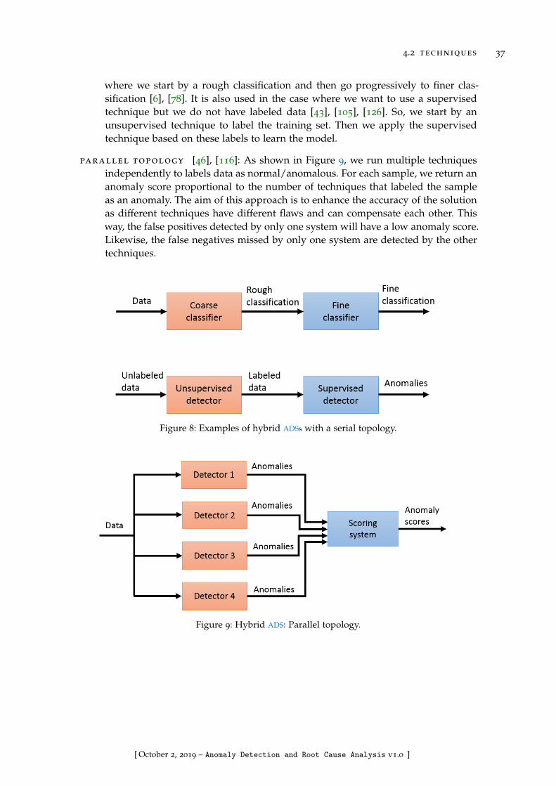
4.2 techniques 37
where we start by a rough classification and then go progressively to finer clas-sification [6], [78]. It is also used in the case where we want to use a supervisedtechnique but we do not have labeled data [43], [105], [126]. So, we start by anunsupervised technique to label the training set. Then we apply the supervisedtechnique based on these labels to learn the model.
parallel topology [46], [116]: As shown in Figure 9, we run multiple techniquesindependently to labels data as normal/anomalous. For each sample, we return ananomaly score proportional to the number of techniques that labeled the sampleas an anomaly. The aim of this approach is to enhance the accuracy of the solutionas different techniques have different flaws and can compensate each other. Thisway, the false positives detected by only one system will have a low anomaly score.Likewise, the false negatives missed by only one system are detected by the othertechniques.
Figure 8: Examples of hybrid ADSs with a serial topology.
Figure 9: Hybrid ADS: Parallel topology.
[ October 2, 2019 – Anomaly Detection and Root Cause Analysis v1.0 ]

38 state of the art
4.3 evaluation methods
In this section, we give an overview of the evaluation methods that can be used to assessthe performance of an ADS.
4.3.1 Confusion Matrix
A confusion matrix is a table that puts together the results of the application of an ML
algorithm. In the case of a anomaly detection (and any binary classification in general),we have four quantities in the confusion matrix:
• True Positives (TPs): A TP is an anomaly labeled correctly by the ADS.
• False Positives (FPs): A FP (called also Type I error) is a normal value labeled erro-neously by the ADS as an anomaly.
• True Negatives (TNs): A TN is a normal value labeled correctly by the ADS.
• False Negatives (FNs): A FN (called also Type II error) is an anomaly labeled erro-neously by the ADS as a normal value.
Predicted
Positive Negative
RealPositive TP FN
Negative FP TN
Table 2: Confusion matrix.
As Table 2 shows, the confusion matrix gives an overview of the performance ofan ADS. Many performance measures have been derived from the confusion matrix toevaluate the accuracy of the results.
4.3.2 Evaluation Metrics
The following measures allow to evaluate the accuracy of an ADS [128]:
specificity : Called also True Negative Rate (TNR), it measures the proportion of nor-mal points that are correctly labeled.
TNR =TN
TN + FP(9)
precision : Called also Positive Predictive Value (PPV), it measures the proportion ofanomalies correctly labeled among all the points predicted as anomalies.
PPV =TP
TP + FP(10)
This measure quantifies the relevance of the points detected as anomalies.
[ October 2, 2019 – Anomaly Detection and Root Cause Analysis v1.0 ]

4.3 evaluation methods 39
recall : Called also sensitivity or True Positive Rate (TPR), it measure the proportionof anomalies that are correctly labeled.
TPR =TP
TP + FN(11)
This measure quantifies the capability of an ADS to detect existing anomalies.
fallout : Called also False Positive Rate (FPR), it measures the proportion of falsepositives among all the normal points.
FPR =FP
FP + TN(12)
False Negative Rate (FNR): is the proportion of not detected anomalies.
FNR =FN
FN + TP(13)
accuracy (ACC): Is the proportion of the points correctly labeled by the ADS.
Accuracy(ACC) =TN + TP
TN + TP + FN + FP(14)
The specificity and the fallout are complementary. They measure the capacity of thesystem to recognize a normal point. Likewise, the recall and the FNR are complementary.They measure the capacity of the system to detect an anomalous point.
TNR + FPR = 1 (15)
TPR + FNR = 1 (16)
4.3.3 Evaluation Curves
4.3.3.1 The Receiver Operating Characteristic curve
Receiver Operating Characteristic (ROC) curve is a plot highlighting the discriminationcapacity of an ADS to distinguish between normal and anomalous points [29]. As shownin Figure 10, the ROC curve plots the TPR as a function of the FPR. The closer the curveto the horizontal asymptote, the better the ADS performance. To compare two ADSs, wemay use the Area Under the Curve (AUC) [16]. A perfect ADS has an AUC = 1. An ADS
with an AUC = 0.5 (orange line in Figure 10) is a random system with no discriminationcapacity.
4.3.3.2 The Precision-Recall curve
The Precision-Recall (PR) curve is another way to assess the quality of an ADS [29]. ThePR curve displays the TPR as a function of the PPV. Like the ROC curve, the PR curve aimsto show the trade-off between detecting all the anomalies and having few false positives.However, as the number of anomalies is in general very low compared to the number ofnormal instances, the FPR can be very close to 0 and its variations can be imperceptible.That is why the use of PPV instead is more judicious.
[ October 2, 2019 – Anomaly Detection and Root Cause Analysis v1.0 ]

40 state of the art
0.0 0.2 0.4 0.6 0.8 1.00.0
0.2
0.4
0.6
0.8
1.0
FPR
TPR
AUC=0.604
Figure 10: An example of a ROC curve.
0 0.2 0.4 0.6 0.8 10
0.2
0.4
0.6
0.8
1
PPV
TPR
Figure 11: An example of a PR curve.
[ October 2, 2019 – Anomaly Detection and Root Cause Analysis v1.0 ]

4.4 summary 41
4.3.4 Validation Techniques
Several techniques are available to validate the results of an ADS and compute the differ-ent performance measures. We present a few examples in the following.
holdout [80]: is the simplest approach to evaluate the performance of an ADS. Wesplit the data set into two non overlapping subsets: a training set and a test set.We learn the model based on the training set. Then, we apply the model to thetest set and compute the performance measures. This way, we make sure that themodel does not over-fit the training set. This approach however, can be biased if thetraining and test set have different distributions and thus are not representative ofthe overall data. For this reason, one should apply stratification, which is splittingdata sets into subsets with the same probability distribution.
cross validation [80]: is a well known technique to validate ML models. It consistsin splitting the data set into k folds. Then, each time, we use k− 1 folds for thetraining and the remaining fold for the test. For each iteration, we compute theperformance measures. The overall performance measures are the averages of theperformance measures of all the iterations. Cross validation reduces the bias of per-formance measures estimation. To have a more accurate evaluation, one may usestratified cross validation which allows to have k subsets with the same probabilitydistribution.
bootstrapping [80]: consists in randomly selecting training instances with replace-ment. The remaining instances that were not included in the training set form thetest set. In this technique, the size of the test set changes depending on the numberof duplicates, triplicates, etc in the training set. This process is repeated and eachtime, one computes the performance metrics. As for cross validation, the overallperformance metrics are the averages of the performance metrics of all iterations.
4.4 summary
In this chapter, we have discussed some of the different approaches the researchers haveapplied to address the question of anomaly detection. As shown in Table 3, many so-lutions with different characteristics have been proposed. Depending on the context,anomaly detection is applied to different data structures and returns different outputs.Learning may be supervised or unsupervised depending on the use case and the avail-ability of labeled training data. Some of the algorithms process data in a simple andintuitive way which makes the results easy to control and interpret. Others are morecomplex and less manageable. The time complexities of the learning phase and the de-tection phases vary drastically from one algorithm to another. In some fields, the train-ing phase is executed very often. Therefore, one should select an algorithm with lowtraining computation needs. In other cases, especially in the mobile networking field,the algorithm should detect anomalies in real time. So, the detection time should bebounded. The algorithms complexity depends not only on the data size and dimension-ality but also on the algorithm parameters. Some parameters, like the number of epochs(iterations) in the case of neural networks and EM algorithm may increase drastically
[ October 2, 2019 – Anomaly Detection and Root Cause Analysis v1.0 ]

42 state of the art
the complexity of the process. The accuracy aspect is not presented in Table 3 as theaccuracy of an algorithm depends tightly on the statistical characteristics of data. An al-gorithm may have a high accuracy in the case of a specific data distribution and performpoorly in another. The thresholding and the configuration aspect in general are to takeinto account when selecting an anomaly detection solution. Generally speaking, there isnot an optimal configuration that fits all data types types and use cases.
[ October 2, 2019 – Anomaly Detection and Root Cause Analysis v1.0 ]
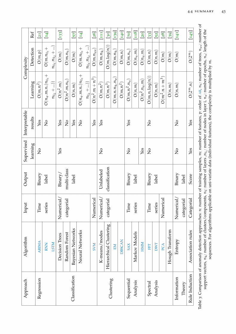
4.4 summary 43
App
roac
hA
lgor
ithm
Inpu
tO
utpu
tSu
perv
ised
Inte
rpre
tabl
eC
ompl
exit
y
lear
ning
resu
lts
Lear
ning
Det
ecti
onR
ef
Reg
ress
ion
AR
IMA
Tim
eBi
nary
No
Yes
O(m
.n2)
O(m
.p)
[21]
RN
Nse
ries
labe
lN
oO(ne
.m.n
.(nl 1+
O(m
.nl 1+
[14]
LSTM
nl 2+
...))
nl 1
.nl 2+
...)
Cla
ssifi
cati
on
Dec
isio
nTr
ees
Num
eric
al/
Bina
ry/
Yes
Yes
O(n2
.m)
O(m
)[1
33]
Ran
dom
Fore
stca
tego
rial
mul
ti-c
lass
No
O(n2
.m.nt)
O(m
.nt)
Baye
sian
Net
wor
ksla
bel
Yes
O(n
.m)
O(m
)[5
7]
Neu
ralN
etw
orks
No
O(ne
.m.n
.(nl 1+
O(m
.nl 1+
[14]
nl 2+
...))
nl 1
.nl 2+
...)
SVM
Num
eric
alYe
sO(n2
.m+n3)
O(m
.nsv)
[26]
Clu
ster
ing
K-m
eans
/mod
esN
umer
ical
/U
nlab
eled
No
Yes
O(m
.n2)
O(m
.nk)
[111]
Hie
rarc
hica
lClu
ster
ing
cate
gori
alcl
assi
ficat
ion
O(m
.n3)
O(m
.log(n
))[3
0]
EMO(m
.n.nk
.ne)
O(m
.nk)
[139]
DBS
CA
NO(m
.n2)
O(m
.n)
[140]
Sequ
enti
alSA
XTi
me
Bina
ryN
oYe
sO(m
.n2
.ns)
O(m
.ns)
[70]
Ana
lysi
sM
arko
vM
odel
sse
ries
labe
lO(n
.m)
O(ns.m
)[1
18]
HM
MYe
sO(n2
.ns.m
)O(ns.m
)[2
0]
Spec
tral
FFT
Tim
eBi
nary
No
No
O(m
.n.log(n
))O(m
.n)
[33]
Ana
lysi
sD
WT
seri
esla
bel
O(n
.m)
O(n
.m)
[52]
PCA
Num
eric
alO(m2
.n+m3)
O(m
)[2
8]
Hou
ghTr
ansf
orm
O(n
.m)
O(m
)[3
9]
Info
rmat
ion
Entr
opy
Num
eric
al/
Bina
ryN
oN
oO(n
.m)
O(m
)[1
41]
Theo
ryca
tego
rial
labe
l
Rul
eIn
duct
ion
Ass
ocia
tion
rule
sC
ateg
oria
lSc
ore
Yes
Yes
O(2m
.n)
O(2m)
[145]
Tabl
e3
:Com
pari
son
ofan
omal
yde
tect
ion
appr
oach
es:n
:num
ber
oftr
aini
ngsa
mpl
es,m
:num
ber
offe
atur
es,p
:ord
erof
AR
,nt:n
umbe
rof
tree
s,nsv
:num
ber
ofsu
ppor
tve
ctor
s,nk
:num
ber
ofcl
uste
rs/c
ompo
nent
s,nl:n
umbe
rof
laye
rs,nl i
:num
ber
ofno
des
inla
yer
i,ne
:num
ber
ofep
ochs
,ns:l
engt
hof
the
sequ
ence
s.Fo
ral
gori
thm
sap
plic
able
onun
i-va
riat
eda
ta(i
ndiv
idua
lfea
ture
s),t
heco
mpl
exit
yis
mul
tipl
ied
bym
.
[ October 2, 2019 – Anomaly Detection and Root Cause Analysis v1.0 ]

[ October 2, 2019 – Anomaly Detection and Root Cause Analysis v1.0 ]
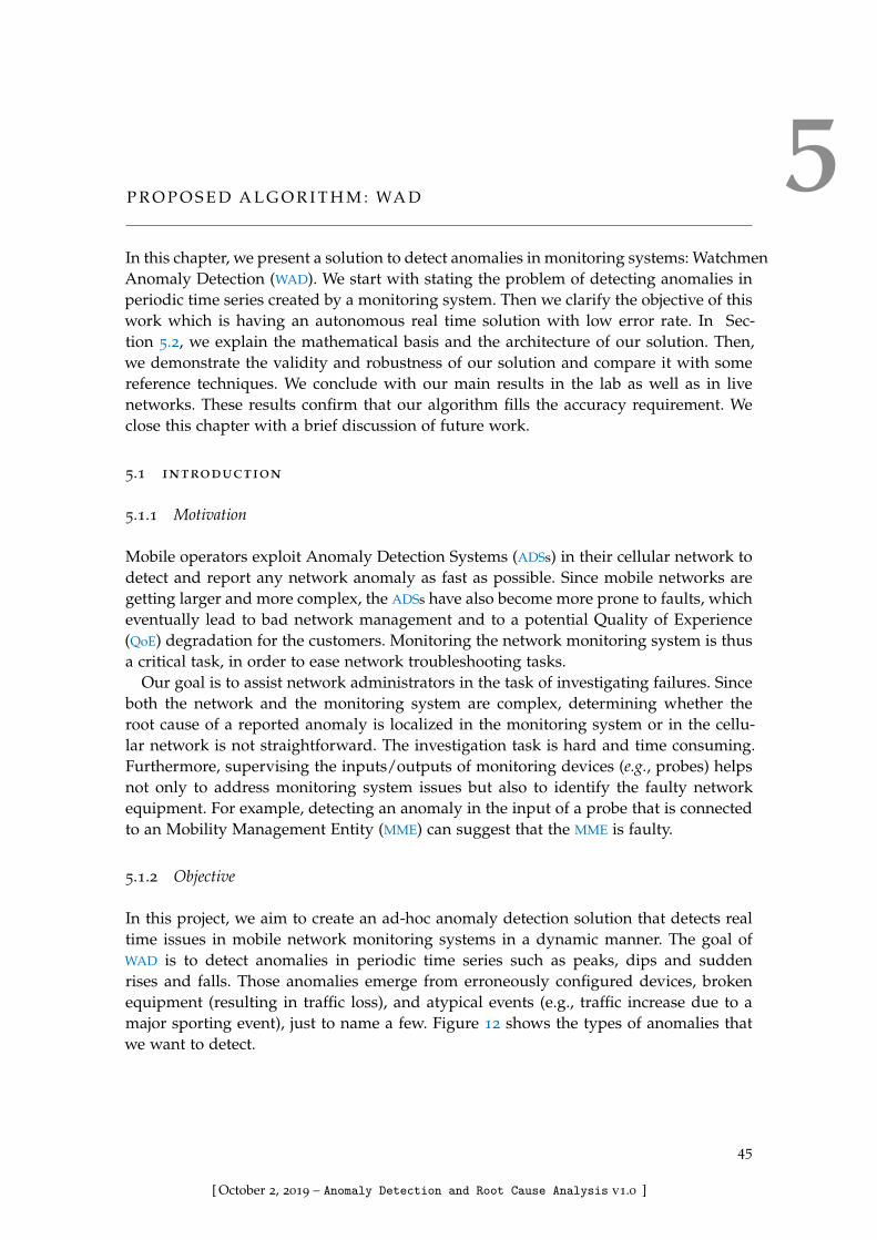
5P R O P O S E D A L G O R I T H M : WA D
In this chapter, we present a solution to detect anomalies in monitoring systems: WatchmenAnomaly Detection (WAD). We start with stating the problem of detecting anomalies inperiodic time series created by a monitoring system. Then we clarify the objective of thiswork which is having an autonomous real time solution with low error rate. In Sec-tion 5.2, we explain the mathematical basis and the architecture of our solution. Then,we demonstrate the validity and robustness of our solution and compare it with somereference techniques. We conclude with our main results in the lab as well as in livenetworks. These results confirm that our algorithm fills the accuracy requirement. Weclose this chapter with a brief discussion of future work.
5.1 introduction
5.1.1 Motivation
Mobile operators exploit Anomaly Detection Systems (ADSs) in their cellular network todetect and report any network anomaly as fast as possible. Since mobile networks aregetting larger and more complex, the ADSs have also become more prone to faults, whicheventually lead to bad network management and to a potential Quality of Experience(QoE) degradation for the customers. Monitoring the network monitoring system is thusa critical task, in order to ease network troubleshooting tasks.
Our goal is to assist network administrators in the task of investigating failures. Sinceboth the network and the monitoring system are complex, determining whether theroot cause of a reported anomaly is localized in the monitoring system or in the cellu-lar network is not straightforward. The investigation task is hard and time consuming.Furthermore, supervising the inputs/outputs of monitoring devices (e.g., probes) helpsnot only to address monitoring system issues but also to identify the faulty networkequipment. For example, detecting an anomaly in the input of a probe that is connectedto an Mobility Management Entity (MME) can suggest that the MME is faulty.
5.1.2 Objective
In this project, we aim to create an ad-hoc anomaly detection solution that detects realtime issues in mobile network monitoring systems in a dynamic manner. The goal ofWAD is to detect anomalies in periodic time series such as peaks, dips and suddenrises and falls. Those anomalies emerge from erroneously configured devices, brokenequipment (resulting in traffic loss), and atypical events (e.g., traffic increase due to amajor sporting event), just to name a few. Figure 12 shows the types of anomalies thatwe want to detect.
45
[ October 2, 2019 – Anomaly Detection and Root Cause Analysis v1.0 ]
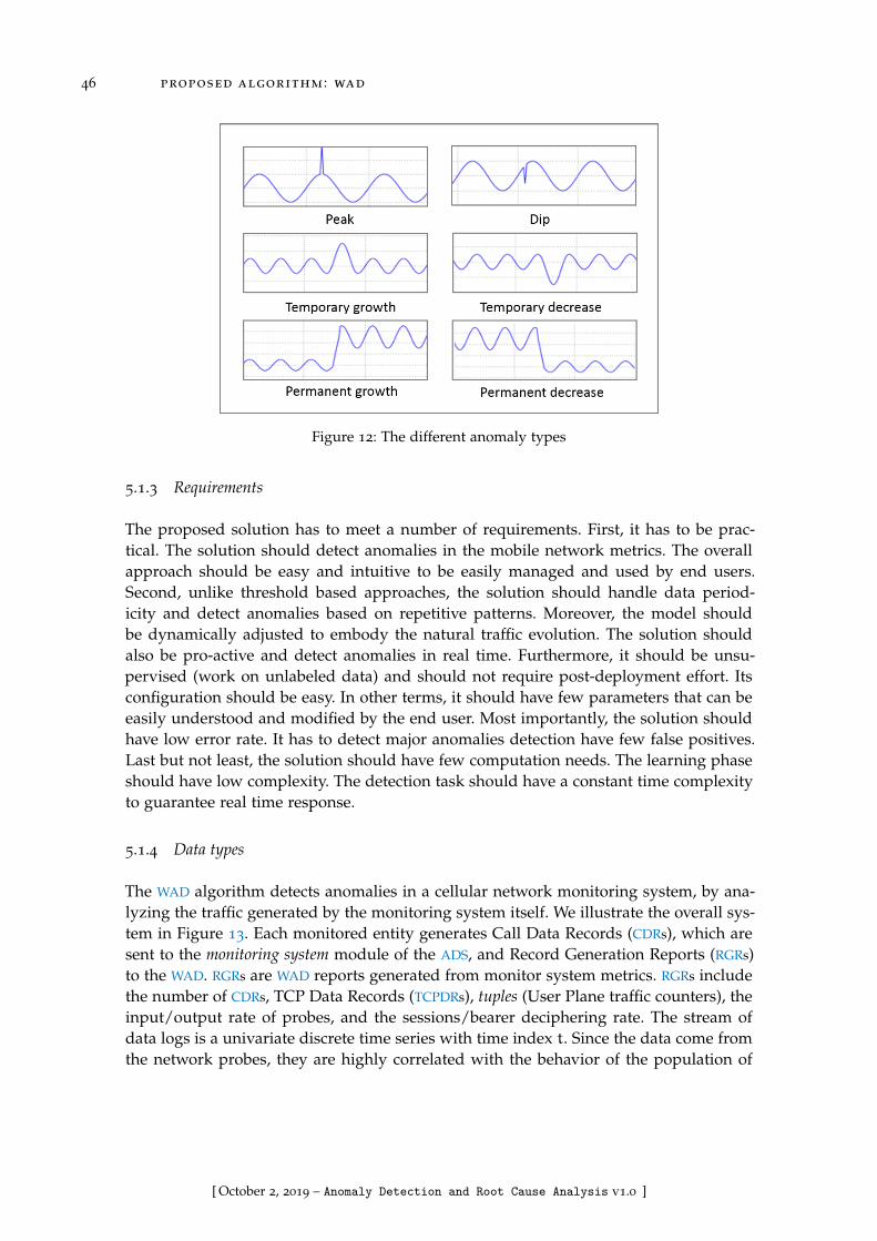
46 proposed algorithm : wad
Figure 12: The different anomaly types
5.1.3 Requirements
The proposed solution has to meet a number of requirements. First, it has to be prac-tical. The solution should detect anomalies in the mobile network metrics. The overallapproach should be easy and intuitive to be easily managed and used by end users.Second, unlike threshold based approaches, the solution should handle data period-icity and detect anomalies based on repetitive patterns. Moreover, the model shouldbe dynamically adjusted to embody the natural traffic evolution. The solution shouldalso be pro-active and detect anomalies in real time. Furthermore, it should be unsu-pervised (work on unlabeled data) and should not require post-deployment effort. Itsconfiguration should be easy. In other terms, it should have few parameters that can beeasily understood and modified by the end user. Most importantly, the solution shouldhave low error rate. It has to detect major anomalies detection have few false positives.Last but not least, the solution should have few computation needs. The learning phaseshould have low complexity. The detection task should have a constant time complexityto guarantee real time response.
5.1.4 Data types
The WAD algorithm detects anomalies in a cellular network monitoring system, by ana-lyzing the traffic generated by the monitoring system itself. We illustrate the overall sys-tem in Figure 13. Each monitored entity generates Call Data Records (CDRs), which aresent to the monitoring system module of the ADS, and Record Generation Reports (RGRs)to the WAD. RGRs are WAD reports generated from monitor system metrics. RGRs includethe number of CDRs, TCP Data Records (TCPDRs), tuples (User Plane traffic counters), theinput/output rate of probes, and the sessions/bearer deciphering rate. The stream ofdata logs is a univariate discrete time series with time index t. Since the data come fromthe network probes, they are highly correlated with the behavior of the population of
[ October 2, 2019 – Anomaly Detection and Root Cause Analysis v1.0 ]
5.2 the wad algorithm 47
subscribers (e.g., they show a daily pattern). In the remainder of the paper we use aperiod of one day but WAD works with any period length.
MME
MME
p1
p2Core Network
MonitoringSystem
WAD
ADS
CDR
RGR
Figure 13: Overall Architecture: two probes p1 and p2 monitor MMEs and send reports to the ADS
5.2 the Watchmen Anomaly Detection algorithm
Watchmen Anomaly Detection (WAD) is an ad-hoc solution to the network anomalydetection problem. It is dynamic and adapts to the natural traffic evolution. It runs inreal time on data coming from monitoring devices, such as network probes measuringtraffic throughput in network interfaces. Based on these measurements (time series), theADS creates reference patterns describing data in normal state. Then it measures thegap between the reference pattern and real time data. If the gap is large, the networkadministrator is notified about an anomaly occurring in the related equipment.
WAD consists of two phases: a learning phase and a detection phase. The learningpart of the algorithm is executed once a day (i.e., the period of the data). In this phase,we create a reference model, which is stored in a database. This reference model is thenused in the detection phase, which runs in real time. Before running the algorithm, thereis a pre-processing step to fill missing values and have the same time interval betweenconsecutive samples. To do so, we apply a simple linear interpolation.
In the following, we will use the metric in Figure 14 to explain the different steps ofWAD. As in the real world process, we will use the 29 first days to build the model andwill apply the detection procedure to the 30th day.
5.2.1 Learning Phase
Figure 15 shows the four main steps of the learning phase, whose input is one monthworth of data for each metric (time series). Note that WAD handles each metric indepen-dently of the others: if we use 40 metrics, we run the learning phase 40 times to produce40 reference models.
5.2.1.1 Periodicity Check
We compute the Fourier transform of the time series to check whether the data is pe-riodic, in which case there is dominant frequency (equal to the inverse of the period)
[ October 2, 2019 – Anomaly Detection and Root Cause Analysis v1.0 ]

48 proposed algorithm : wad
Figure 14: The CDR number at an output interface of a hub.
Daily patternDoM
transformThresholding
Periodicitycheck
Manualsupervision
Database
RGRi NO
YES
pattern
RGRi
patterntransform
RGRitransform
patterntransform
threshold
Figure 15: The learning phase for a metric RGRi
[ October 2, 2019 – Anomaly Detection and Root Cause Analysis v1.0 ]
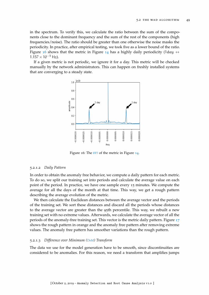
5.2 the wad algorithm 49
in the spectrum. To verify this, we calculate the ratio between the sum of the compo-nents close to the dominant frequency and the sum of the rest of the components (highfrequencies/noise). The ratio should be greater than one otherwise the noise masks theperiodicity. In practice, after empirical testing, we took five as a lower bound of the ratio.Figure 16 shows that the metric in Figure 14 has a highly daily periodicity (1day ↔1.157× 10⁻⁵Hz).
If a given metric is not periodic, we ignore it for a day. This metric will be checkedmanually by the network administrators. This can happen on freshly installed systemsthat are converging to a steady state.
Figure 16: The FFT of the metric in Figure 14.
5.2.1.2 Daily Pattern
In order to obtain the anomaly free behavior, we compute a daily pattern for each metric.To do so, we split our training set into periods and calculate the average value on eachpoint of the period. In practice, we have one sample every 15 minutes. We compute theaverage for all the days of the month at that time. This way, we get a rough patterndescribing the average evolution of the metric.
We then calculate the Euclidean distances between the average vector and the periodsof the training set. We sort these distances and discard all the periods whose distancesto the average vector are greater than the 95th percentile. This way, we rebuilt a newtraining set with no extreme values. Afterwards, we calculate the average vector of all theperiods of the anomaly-free training set. This vector is the metric daily pattern. Figure 17
shows the rough pattern in orange and the anomaly free pattern after removing extremevalues. The anomaly free pattern has smoother variations than the rough pattern.
5.2.1.3 Difference over Minimum (DoM) Transform
The data we use for the model generation have to be smooth, since discontinuities areconsidered to be anomalies. For this reason, we need a transform that amplifies jumps
[ October 2, 2019 – Anomaly Detection and Root Cause Analysis v1.0 ]

50 proposed algorithm : wad
Figure 17: Daily pattern:Rough pattern and anomly free pattern after removing extreme values.
and minimizes smooth variations. To this end, we define the DoM transform (T ) of afunction f as:
T(f,L) = d (f (t) , f (t− L)) (17)
where d is defined as:d(x,y) =
x− y
min(x,y)(18)
and L > 0 is the order of the transform (the lag between the two samples of f). Thistransform quantifies the jumps in f after L time steps, starting from a given time t. Inthe remainder of this paper, we focus on the transform of first order since it acts likea derivative and it features that it goes to infinity when there is a peak (or a dip) andit sticks to small values otherwise. Figure 18 shows the DoM transform applied to themetric in Figure 14.
In this phase, we calculate the DoM transform of the metric and the DoM transform ofits daily pattern.
5.2.1.4 Thresholding
At this point of the algorithm, we measure the distance between the transformed valueof each sample of the metric and the corresponding (with regard to the time of theday) transformed value of the pattern. The histogram of distances in Figure 19 showsthat most of the distances between the transformed training data and the transformedpattern are close to 0 as expected. We sort these distances and we set the threshold tothe 99th percentile.
We store the threshold and the DoM transform of the daily pattern in the database forreal time detection phase.
[ October 2, 2019 – Anomaly Detection and Root Cause Analysis v1.0 ]

5.2 the wad algorithm 51
Figure 18: DoM transform applied to the metric in Figure 14.
Figure 19: The histogram of distances between the transformed training data and the trans-formed pattern.
[ October 2, 2019 – Anomaly Detection and Root Cause Analysis v1.0 ]
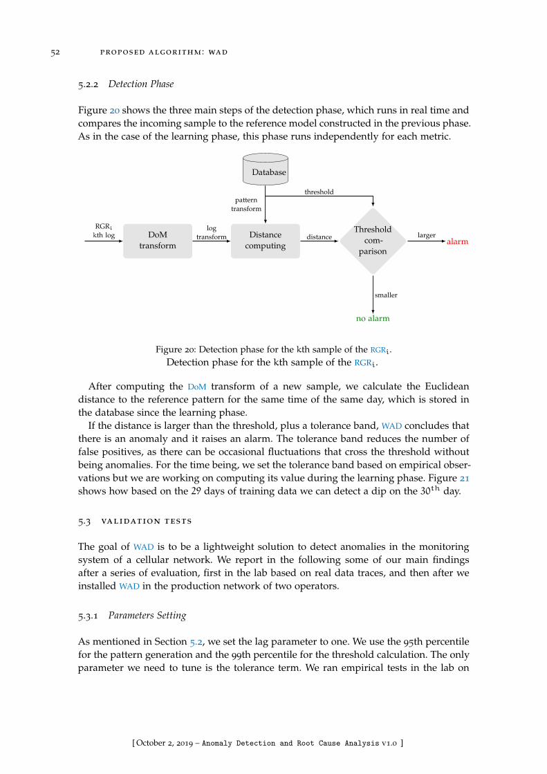
52 proposed algorithm : wad
5.2.2 Detection Phase
Figure 20 shows the three main steps of the detection phase, which runs in real time andcompares the incoming sample to the reference model constructed in the previous phase.As in the case of the learning phase, this phase runs independently for each metric.
DoMtransform
Distancecomputing
Database
Thresholdcom-
parisonalarm
no alarm
RGRikth log
logtransform
patterntransform
threshold
distance larger
smaller
Figure 20: Detection phase for the kth sample of the RGRi.Detection phase for the kth sample of the RGRi.
After computing the DoM transform of a new sample, we calculate the Euclideandistance to the reference pattern for the same time of the same day, which is stored inthe database since the learning phase.
If the distance is larger than the threshold, plus a tolerance band, WAD concludes thatthere is an anomaly and it raises an alarm. The tolerance band reduces the number offalse positives, as there can be occasional fluctuations that cross the threshold withoutbeing anomalies. For the time being, we set the tolerance band based on empirical obser-vations but we are working on computing its value during the learning phase. Figure 21
shows how based on the 29 days of training data we can detect a dip on the 30th day.
5.3 validation tests
The goal of WAD is to be a lightweight solution to detect anomalies in the monitoringsystem of a cellular network. We report in the following some of our main findingsafter a series of evaluation, first in the lab based on real data traces, and then after weinstalled WAD in the production network of two operators.
5.3.1 Parameters Setting
As mentioned in Section 5.2, we set the lag parameter to one. We use the 95th percentilefor the pattern generation and the 99th percentile for the threshold calculation. The onlyparameter we need to tune is the tolerance term. We ran empirical tests in the lab on
[ October 2, 2019 – Anomaly Detection and Root Cause Analysis v1.0 ]
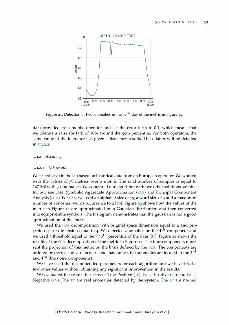
5.3 validation tests 53
Figure 21: Detection of two anomalies in the 30th day of the metric in Figure 14.
data provided by a mobile operator and set the error term to 0.1, which means thatwe tolerate a raise (or fall) of 10% around the 99th percentile. For both operators, thesame value of the tolerance has given satisfactory results. These latter will be detailedin 5.3.2.2.
5.3.2 Accuracy
5.3.2.1 Lab results
We tested WAD in the lab based on historical data from an European operator. We workedwith the values of 58 metrics over a month. The total number of samples is equal to167 040with 90 anomalies. We compared our algorithm with two other solutions suitablefor our use case: Symbolic Aggregate Approximation (SAX) and Principal ComponentAnalysis (PCA). For SAX, we used an alphabet size of 15, a word size of 4 and a maximumnumber of abnormal words occurrence to 2 [70]. Figure 23 shows how the values of themetric in Figure 14 are approximated by a Gaussian distribution and then convertedinto equiprobable symbols. The histogram demonstrates that the gaussian is not a goodapproximation of this metric.
We used the PCA decomposition with original space dimension equal to 4 and pro-jection space dimension equal to 4. We detected anomalies on the 4th component andwe used a threshold equal to the 99.5th percentile of the data [81]. Figure 22 shows theresults of the PCA decomposition of the metric in Figure 14. The four components repre-sent the projection of this metric on the basis defined by the PCA. The components areordered by decreasing variance. As one may notice, the anomalies are located in the 3rd
and 4th (the noise components).We have used the recommended parameters for each algorithm and we have tried a
few other values without obtaining any significant improvement in the results.We evaluated the results in terms of True Positive (TP), False Positive (FP) and False
Negative (FN). The TP are real anomalies detected by the system. The FP are normal
[ October 2, 2019 – Anomaly Detection and Root Cause Analysis v1.0 ]
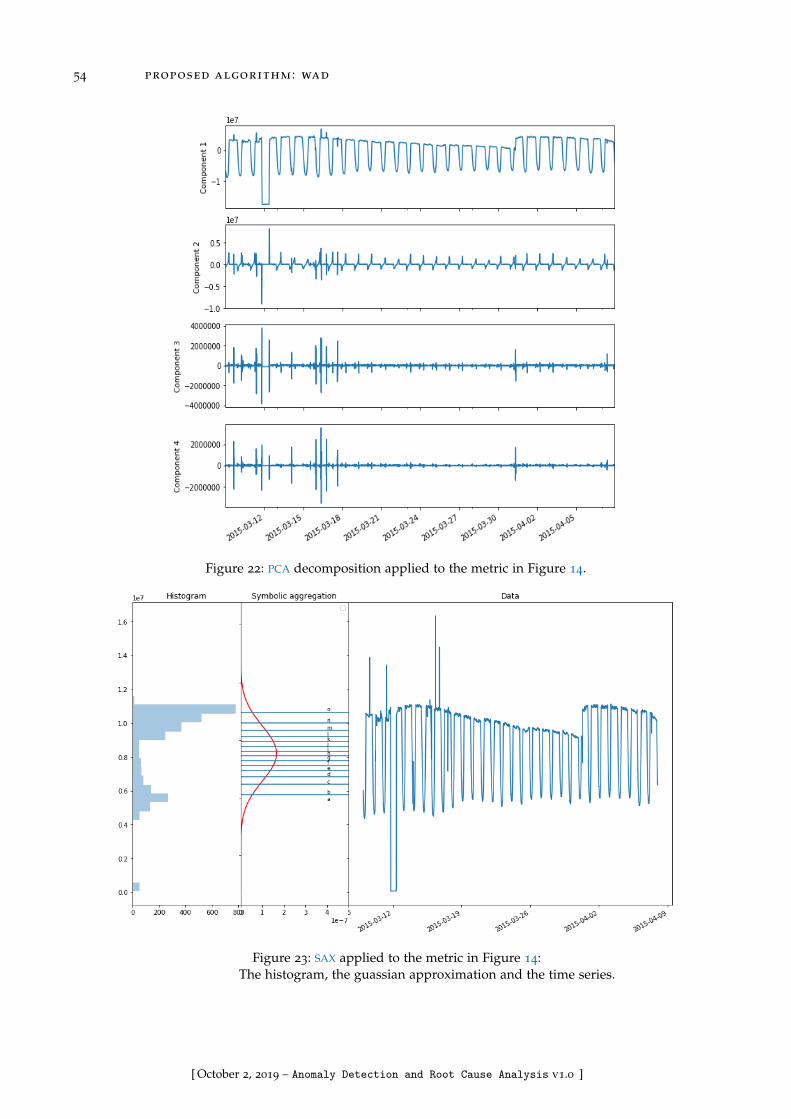
54 proposed algorithm : wad
Figure 22: PCA decomposition applied to the metric in Figure 14.
Figure 23: SAX applied to the metric in Figure 14:The histogram, the guassian approximation and the time series.
[ October 2, 2019 – Anomaly Detection and Root Cause Analysis v1.0 ]

5.3 validation tests 55
points erroneously labeled as anomalies. The FN are anomalies not detected by the sys-tem. We also measured the sensitivity, which is the ratio of correctly detected anomaliesto the total number of anomalies, and the specificity, which is the ratio of points correctlyidentified as normal to the total number of normal points. Table 4 shows the results ofthese tests.
Algorithm TP FP FN Sensitivity Specificity
SAX 59 6 31 0.65 0.99
PCA 85 85 5 0.94 0.99
WAD 81 9 9 0.90 0.99
Table 4: Lab Evaluation Results
The results show that the PCA decomposition is a good method to detect abruptchanges. However, it does not fit all types of data. For example, PCA supposes thatthe noise and anomalies are linearly separable from significant data, although it is notalways the case. Another problem with PCA-based anomaly detection is that includinganomalies in the noise component implies a high FPs rate. Another source of uncertaintylies in the fact that the number of noise components depends highly on the metric.When we run our tests, we have noticed that for different metrics in the same data set,anomalies are not in the same component. As previously said, we used a 4-dimensionalprojection space. For some metrics, we detected anomalies only in the third component,for some other metrics in the fourth component and for other different metrics in boththe third and the fourth components. This implies that, in order to have accurate results,one needs the intervention of an expert, who can analyze the data, for each metric, todetermine which component contains the anomalies. Such a solution is not feasible in aproduction environment.
The SAX algorithm obtains a high FN number since SAX does not keep track of time.Thus, it considers some behaviors as being normal although they abnormally took placeat an unusual time (e.g., a peak at 5am while usually there is not peak at that time). Ouralgorithm offers a good trade-off between FPs and FNs rates.
Figures 24,25 and 26 show the Precision-Recall (PR) curves of SAX, PCA and WAD cre-ated using different parameters applied to five metrics selected by experts: a metric withno anomalies, two metrics with few anomalies and two metrics with many anomalies.These curves confirm that SAX has a highest precision , PCA has a highest recall and WAD
give a fair trade off between the two.
5.3.2.2 Live network results
We install WAD during three months to supervise the network of two mobile operators(in Europe and Africa). The first operator gave a general positive feedback, withoutgiving specific numbers. The second one gave us access to a detailed feedback. In theremainder of this section, we will refer to these results. Figure 27 shows an example ofresults given by WAD on the number of tuples at the output of a probe. The dots here arethe anomalies detected by WAD.
[ October 2, 2019 – Anomaly Detection and Root Cause Analysis v1.0 ]

56 proposed algorithm : wad
Figure 24: The PR curve of SAX results.
Figure 25: The PR curve of PCA results.
Figure 26: The PR curve of WAD results.
[ October 2, 2019 – Anomaly Detection and Root Cause Analysis v1.0 ]

5.3 validation tests 57
Figure 27: Anomalies in the number of Tuples – probe output
The network administrator selected 18 metrics and provided feedback about the per-formance of our algorithm. During the three months, 83 anomalies occured (among155 520 samples). We detected 75 of them, which means we had eight false negatives.We also detected four false anomalies. The sensitivity of the system is equal to 0.90 andthe specificity is equal to 0.99. The accuracy of WAD meets the requirements of bothoperators.
5.3.3 Memory and Computation Needs
The step of periodicity check has a complexity of O(nlog(n)) since it is based on FFT [33].Each of the remaining steps of the training phase (pattern creation, DoM transform andthresholding) has a O(n) complexity. Thus, WAD has a O(nlog(n)) complexity, as theFFT is the term with the dominant time complexity. We have evaluated WAD hardwareperformance on a machine with the following features: 4 Cores, 4GB RAM, 30GB harddrive. We have noticed a peak once a day in the CPU utilization related to the learningphase. The training phase takes about 30 minutes to process 850MB of data (we monitor55 metrics, we have one month of data per metric with one sample every 15 minutes).Tables 5 and 6 show the results of these tests.
Median 95th percentile Max
Learning Phase 12% 14% 25%
Detection Phase 0.1% 1% 2%
Table 5: WAD CPU Usage
Based on these experiments and on the successful deployment in production networks,we conclude that WAD has modest requirements in terms of memory and computingpower, even during the learning phase.
[ October 2, 2019 – Anomaly Detection and Root Cause Analysis v1.0 ]

58 proposed algorithm : wad
Median 95th percentile Max
Learning Phase 1.2% 1.5% 1.6%
Detection Phase 0.5% 0.8% 0.9%
Table 6: WAD Memory Usage
5.3.4 Discussion
WAD gives promising results in terms of gain of productivity, time saving, and ease ofoutage troubleshooting. After using WAD for a few months, the network administratorsof two cellular operators have highlighted the following aspects. They have noticed thatthey do not have to check all the metrics manually, since they are alerted in real time.They also save a lot of time and effort in troubleshooting and understanding issues:our algorithm helps them localize the problem and therefore fix broken devices and/orconfigurations efficiently. The configuration of our solution is straightforward since itproduces dynamic models (updated automatically). It does not classify days into work-ing days and holidays, therefore there is no need for calendar integration. Finally, as anadded benefit, it does not require a large training set.
To sum up, automatic supervision of network monitoring systems and real time feed-backs processing is crucial to automatize mobile network troubleshooting. Thus, inte-grating an ADS based on Machine Learning techniques like WAD within a network mon-itor system seems to be an essential task for the creation of self healing networks. Ourresearch may contribute to the definition of basic functions for self-organizing and moreresilient networks.
[ October 2, 2019 – Anomaly Detection and Root Cause Analysis v1.0 ]
6I N D U S T R I A L I Z AT I O N
Watchmen Anomaly Detection (WAD) can be applied to different types of data in dif-ferent contexts. In this Chapter, we detail how we industrialized WAD to achieve twodifferent objectives. The first objective is to automatically monitor the monitoring sys-tem in order to ease the network administrators tasks. The second objective is to helptelecommunication experts to carry out service quality management.
6.1 monitoring the monitoring system : nova cockpit™
In the following, we go through the scoping phase and the deployment phase of inte-grating WAD in Nova Cockpit™.
6.1.1 The scoping phase
Our goal is to implement the WAD algorithm to monitor the monitoring system by in-tegrating it as a plugin of the monitoring tool: Nova Cockpit™. We present here thescope of the project starting by the development environment which is the Cockpit™framework. Then we detail the accessible data for WAD application. We finish by statingthe requirements and constraints of this project.
6.1.1.1 Environment
Cockpit™ is a software designed to monitor EXFO monitoring solution. Figure 28 showshow it collects monitoring metrics that are aggregated measurements of the input/out-put data of probes and other monitoring devices. Network administrators analyze thesemetrics during their daily checks to find issues within the monitoring solution.
Cockpit™ offers straightforward monitoring interfaces containing human readableinformation status. It processes data in real time, centralizes information and createsinteractive graphics. It provides alerting services for probes, applications, switches, etc.It also offers network service monitoring (e.g., for Simple Mail Transfer Protocol (SMTP),File Transfer Protocol (FTP)) and host monitoring (e.g., Central Processing Unit (CPU)load, disk usage).
In this project, we aim to add an anomaly detection plugin based on WAD as a featureof Cockpit™ to monitor the EXFO monitoring system. The plugin has to analyse Cock-pit™ data to detect issues in real time. The plugin will inter-operate with the differentcomponents of Cockpit™.
59
[ October 2, 2019 – Anomaly Detection and Root Cause Analysis v1.0 ]

60 industrialization
Figure 28: EXFO monitoring system.Cockpit™ collects data from Neptune™ probes, Nephub™, and Mediation™
interfaces.
[ October 2, 2019 – Anomaly Detection and Root Cause Analysis v1.0 ]

6.1 monitoring the monitoring system : nova cockpit™ 61
6.1.1.2 Accessible Data
The anomaly detection plugin has to analyze the data collected by Cockpit™ from EXFOmonitoring solution. As Figure 28 shows, the monitoring solution has three main com-ponents:
neptune™ is a passive high capacity probe that captures the traffic for multiple ap-plications such as network optimization, customer care and network managementand supervision. A Neptune™ probe captures and processes huge volumes ofControl Plane (CP) and User Plane (UP) traffic in real-time. It generates Call DataRecords (CDRs) and TCP Data Records (TCPDRs) for key interfaces of core net-work sites such as Mobility Management Entitys (MMEs), Serving GPRS SupportNodes (SGSNs) and Gateway GPRS Support Nodes (GGSNs).
nephub™ is a hub that centralizes configurations for up to 16 Neptune™ probes. Italso aggregates CDRs and TCPDRs.
mediation™ is a software component that processes, enriches and aggregates datainto cubes (aggregated counters). It also provides multidimensional Key Perfor-mance Indicators (KPIs). Nova Mediation™ is designed for Business Intelligenceand Big Data processing aims.
The Nagios scheduler runs services to pull data regularly from the different compo-nents. It queries the components to get the metrics needed to supervise the monitoringsystem. Table 7 details the list of metrics at each interface of the monitoring system. Ourgoal, in this project, is to apply anomaly detection to these metrics to find issues in themonitoring system.
6.1.1.3 Objectives
The main goal of this project is to detect anomalies in the devices monitored by EXFOsolution. The deployed plugin should process data and alert users in real time. It hasto have a low error rate. The plugin should not interfere with Cockpit™ functions andshould not impact Cockpit™ computational performance. The configuration tasks suchas adding new metrics should be straightforward. The plugin should also respect Cock-pit™ plugin architecture in order to ease maintenance operations.
6.1.2 The deployment phase
The anomaly detection plugin has been deployed in two Cockpit™ instances installedin two different networks for two years. The plugin has given promising results in termsof gain of productivity, time saving, and ease of outage troubleshooting. More than100 metrics were supervised on each network. The overall results are satisfactory. Thedetection of false positives and false negatives is relatively rare and no precision issuewas signaled by network administrators. The computational complexity and the CPU andmemory needs are low. The anomaly detection plugin did not have any visible impacton Cockpit™ computational performance. The initial parameters were well tuned. Theyhave been changed only once in one of the networks and not modified in the other.
[ October 2, 2019 – Anomaly Detection and Root Cause Analysis v1.0 ]

62 industrialization
Monitoring component Metrics
Neptune™ Input Rate: Average input rate (Mbps)
Output Rate (CDR+ TCPDR+ BDR):
Average output rate (Mbps)
Nephub™ CDR Input: Number of CDR received per Neptune™ (notcumulative)
CDR Output: Number of CDR sent to each Mediation™ (notcumulative)
TCPDR Input: Number of TCPDR received per Neptune™(not cumulative)
TCPDR Output: Number of TCPDR sent to each Mediation™(not cumulative)
Mediation™ UP CDR Input: Number of CDR received per interface
CDR Output: Number of CDR inserted in the counterdatabase (per interface)
Mediation™ CP TCPDR Input: Number of TCPDR received per interface
SDR Output: Number of SDR inserted in the counterdatabase (per interface)
Table 7: Cockpit™ Metrics by monitoring component.
Figures 29 and 30 are examples of graphs generated by Cockpit™ anomaly detectionplugin. The blue envelope is the pattern plus/minus the threshold (the maximum ac-ceptable distance to the pattern). In the two graphs, it is obvious that the envelope isadapted dynamically to the data which confirms that the algorithm is learning fromnew data.
Figure 29 is a plot of the input rate of a Neptune™ probe captured in September2016. It shows detected dips related to maintenance and configuration issues. The trafficgrowth is detected at end of the graph is due to a new network configuration. Figure 29
is a plot of the number of CDRs at the interface between the Nephub™ and its firstconnected Neptune™ probe captured in November 2017. The graph shows a detectedpeak caused by the change to the winter time in the corresponding country and a diprelated to a maintenance operation.
6.1.3 Sample Use Case
We now describe a specific incident to highlight the efficiency and usefulness of theCockpit™ anomaly detection plugin. The network administrators supervise only a fewmetrics as the number of metrics is large. They also focus on constant metrics as detect-ing problems on them is easier than in periodic metrics. In September 2016, during adaily check, a network administrator detected an important decrease in the decipheringrate which has to be constant around 100%. The graph of the deciphering rate is shownin Figure 31. The anomaly detection plugin had detected an anomaly in the input of
[ October 2, 2019 – Anomaly Detection and Root Cause Analysis v1.0 ]

6.1 monitoring the monitoring system : nova cockpit™ 63
Figure 29: Cockpit™ capture of a Neptune™ probe Input Rate.The envelope of acceptable values is in blue and the detected anomalies in red.
Figure 30: Cockpit™ capture of Nephub™ CDR
Input, at the interface between a Neptune™ probe and the Nephub™.
[ October 2, 2019 – Anomaly Detection and Root Cause Analysis v1.0 ]
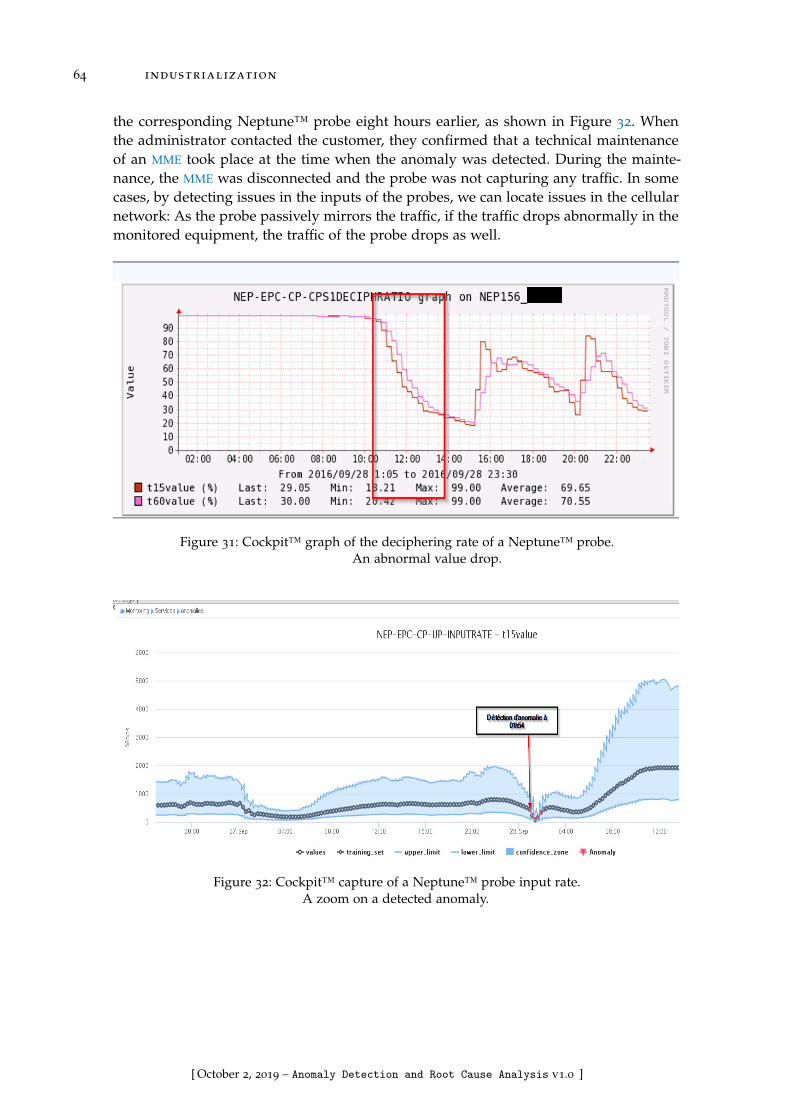
64 industrialization
the corresponding Neptune™ probe eight hours earlier, as shown in Figure 32. Whenthe administrator contacted the customer, they confirmed that a technical maintenanceof an MME took place at the time when the anomaly was detected. During the mainte-nance, the MME was disconnected and the probe was not capturing any traffic. In somecases, by detecting issues in the inputs of the probes, we can locate issues in the cellularnetwork: As the probe passively mirrors the traffic, if the traffic drops abnormally in themonitored equipment, the traffic of the probe drops as well.
Figure 31: Cockpit™ graph of the deciphering rate of a Neptune™ probe.An abnormal value drop.
Figure 32: Cockpit™ capture of a Neptune™ probe input rate.A zoom on a detected anomaly.
[ October 2, 2019 – Anomaly Detection and Root Cause Analysis v1.0 ]
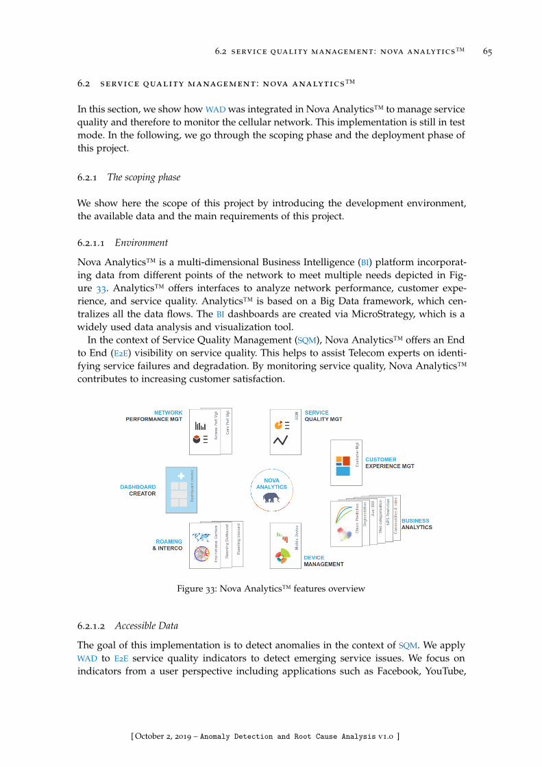
6.2 service quality management : nova analytics™ 65
6.2 service quality management : nova analytics™
In this section, we show how WAD was integrated in Nova Analytics™ to manage servicequality and therefore to monitor the cellular network. This implementation is still in testmode. In the following, we go through the scoping phase and the deployment phase ofthis project.
6.2.1 The scoping phase
We show here the scope of this project by introducing the development environment,the available data and the main requirements of this project.
6.2.1.1 Environment
Nova Analytics™ is a multi-dimensional Business Intelligence (BI) platform incorporat-ing data from different points of the network to meet multiple needs depicted in Fig-ure 33. Analytics™ offers interfaces to analyze network performance, customer expe-rience, and service quality. Analytics™ is based on a Big Data framework, which cen-tralizes all the data flows. The BI dashboards are created via MicroStrategy, which is awidely used data analysis and visualization tool.
In the context of Service Quality Management (SQM), Nova Analytics™ offers an Endto End (E2E) visibility on service quality. This helps to assist Telecom experts on identi-fying service failures and degradation. By monitoring service quality, Nova Analytics™contributes to increasing customer satisfaction.
Figure 33: Nova Analytics™ features overview
6.2.1.2 Accessible Data
The goal of this implementation is to detect anomalies in the context of SQM. We applyWAD to E2E service quality indicators to detect emerging service issues. We focus onindicators from a user perspective including applications such as Facebook, YouTube,
[ October 2, 2019 – Anomaly Detection and Root Cause Analysis v1.0 ]
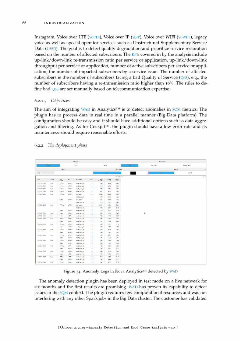
66 industrialization
Instagram, Voice over LTE (VoLTE), Voice over IP (VoIP), Voice over WIFI (VoWIFI), legacyvoice as well as special operator services such as Unstructured Supplementary ServiceData (USSD). The goal is to detect quality degradation and prioritize service restorationbased on the number of affected subscribers. The KPIs covered in by the analysis includeup-link/down-link re-transmission ratio per service or application, up-link/down-linkthroughput per service or application, number of active subscribers per service or appli-cation, the number of impacted subscribers by a service issue. The number of affectedsubscribers is the number of subscribers facing a bad Quality of Service (QoS), e.g., thenumber of subscribers having a re-transmission ratio higher than 10%. The rules to de-fine bad QoS are set manually based on telecommunication expertise.
6.2.1.3 Objectives
The aim of integrating WAD in Analytics™ is to detect anomalies in SQM metrics. Theplugin has to process data in real time in a parallel manner (Big Data platform). Theconfiguration should be easy and it should have additional options such as data aggre-gation and filtering. As for Cockpit™, the plugin should have a low error rate and itsmaintenance should require reasonable efforts.
6.2.2 The deployment phase
Figure 34: Anomaly Logs in Nova Analytics™ detected by WAD
The anomaly detection plugin has been deployed in test mode on a live network forsix months and the first results are promising. WAD has proven its capability to detectissues in the SQM context. The plugin requires few computational resources and was notinterfering with any other Spark jobs in the Big Data cluster. The customer has validated
[ October 2, 2019 – Anomaly Detection and Root Cause Analysis v1.0 ]

6.2 service quality management : nova analytics™ 67
its interest on having WAD as a part of the analysis solution. Another implementation inan additional customer network is planned in 2019.
Figure 34 shows an example of anomalies detected in the SQM context over 24 hoursin July 2018. WAD is applied to cubes from the S1-U interface. The data is aggregatedto a value per hour. We applied two filters: Radio Access Technology (RAT): 4G, ser-vice: Hypertext Transfer Protocol (HTTP) or Youtube. The monitored counters are thenumber of active subscribers and the number of impacted subscriber by bad QoS (highre-transmission ratio and low throughput).
Figure 35 explains four anomalies on the number of subscribers accessing HTTP service.The upper bar-plot contains the number of subscribers accessing HTTP. The black barspresent normal values and the red bars denote anomalies. In "KPIs trend" rectangle, theblue and the gray curves denote respectively the up-link throughput and the down-linkthroughput. The lower bar-plot in red denotes the up-link Transmission Control Protocol(TCP) re-transmission. In this graph, we see that the first three anomalies (detected on2018/07/15) coincide with peaks in the up-link re-transmission. This means that thenumber of subscribers accessing HTTP increased because of an up-link re-transmissionissue. The last anomaly (detected on 2018/07/16) coincides with a decrease in the up-link throughput as well as in the down-link throughput. Thus, this anomaly results froma traffic issue. In this figure, the re-transmission bar-plot and the throughput curvesconfirm that the detected anomalies on the number of impacted subscribers are truepositives.
Figure 35: HTTP monitoring.The number of impacted subscribers compared to the throughput and
re-transmission KPIs. Anomalies detected in the number of impacted subscribers.
Figure 36 presents the same KPIs for Youtube service. This figure shows two anomalieson the number of impacted subscribers accessing Youtube (detected on 2018/07/13 and
[ October 2, 2019 – Anomaly Detection and Root Cause Analysis v1.0 ]
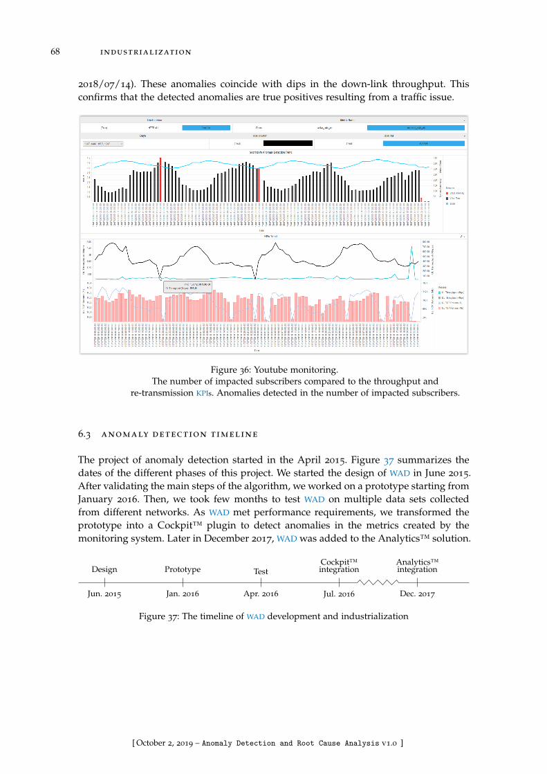
68 industrialization
2018/07/14). These anomalies coincide with dips in the down-link throughput. Thisconfirms that the detected anomalies are true positives resulting from a traffic issue.
Figure 36: Youtube monitoring.The number of impacted subscribers compared to the throughput and
re-transmission KPIs. Anomalies detected in the number of impacted subscribers.
6.3 anomaly detection timeline
The project of anomaly detection started in the April 2015. Figure 37 summarizes thedates of the different phases of this project. We started the design of WAD in June 2015.After validating the main steps of the algorithm, we worked on a prototype starting fromJanuary 2016. Then, we took few months to test WAD on multiple data sets collectedfrom different networks. As WAD met performance requirements, we transformed theprototype into a Cockpit™ plugin to detect anomalies in the metrics created by themonitoring system. Later in December 2017, WAD was added to the Analytics™ solution.
Jun. 2015
Design
Jan. 2016
Prototype
Apr. 2016
Test
Jul. 2016
Cockpit™integration
Dec. 2017
Analytics™integration
Figure 37: The timeline of WAD development and industrialization
[ October 2, 2019 – Anomaly Detection and Root Cause Analysis v1.0 ]

6.4 conclusion 69
6.4 conclusion
In this chapter, we have showed how WAD was integrated in commercialized products todetect anomalies for two different aims. The first objective is to monitor the monitoringsystem. The implementation and tests demonstrate that WAD is effective in supervisingboth hardware and software components of the monitoring system. WAD was also usedto monitor the cellular network by detecting anomalies in QoS indicators. The first resultsare promising. These implementations in industrial products has proved that WAD is avalid solution to detect anomalies in periodic time series in the context of monitoringcellular networks.
[ October 2, 2019 – Anomaly Detection and Root Cause Analysis v1.0 ]

[ October 2, 2019 – Anomaly Detection and Root Cause Analysis v1.0 ]

Part III
R O O T C A U S E D I A G N O S I S
This part is about the second objective of the thesis: Root cause diagnosis.In this part, we start by a study of the state of the art. Then, we propose asolution for this question and evaluate its performance. We finish by a shortdescription of the industrialization process.
[ October 2, 2019 – Anomaly Detection and Root Cause Analysis v1.0 ]

[ October 2, 2019 – Anomaly Detection and Root Cause Analysis v1.0 ]
7S TAT E O F T H E A RT
In this chapter, we present the state of the art of root cause diagnosis. We start bystating the problem. Then, we explore the different approaches proposed to deal withthis question. Finally, we give an overview of the proposed solutions to perform rootcause diagnosis.
7.1 problem statement
After detecting anomalies, the natural step towards healing the network is the diag-nosis of the anomaly. This step aims at accurately identifying the origin of the error,which allows operators to take the appropriate mitigation actions. In a cellular network,anomalies can be related to the network itself such as radio interference between cells.Anomalies can also be related to subscribers such as Operating System (OS) bugs orto service providers such as routing issues. In the literature, the diagnosis process hastaken various denominations in the research history such as "Root cause diagnosis","Fault diagnosis" and "Fault localization". These titles refer to the process of identifyingand delimiting the elements originating the anomaly. The question of root cause diag-nosis has been studied in different domains for at least three decades. However, morework need to be carried out as this process still rely on human expertise in a major part.As a matter of fact, identifying the root of an anomaly requires a good knowledge ofthe domain, the anomaly context and the historical data: In concrete terms, a humanexpert analyses the context and the historical data to infer the possible causes of an is-sue. Designing a system capable of carrying out this analysis is very challenging. Thesystem has to have the intelligence to perform a coherent analysis and the memory tolearn from past experiences in a dynamic way. The current state of the art shows thatmany researchers have tried to address this question from different perspective. Theyproposed a wide variety of approaches differing in may aspects: domain-dependence,level of automation, context-awareness, analysis depth, etc. In this chapter, we aim toexamine the main proposed approaches.
As stated in [121], the root cause diagnosis task can be based on different types ofinformation. The different types of data are used by both human experts and monitoringsystems to analyse issues and identify their root causes. To start with, network alarmsmay help in localizing the root cause of issues. The alarms indicate errors in networkelements. The element concerned with the alarm is not necessarily the root of the issueand the alarm could be a mere result of an underlying breakdown. Multiple alarms atdifferent point of the network may allow to diagnose the nature of the root problem.Moreover, status monitoring may produce data relevant to the diagnosis task. By ana-lyzing the historical status of each of the network elements, experts are able to delimitthe extent of an issue and understand its roots. These data can be found in the net-work logs/traces. Furthermore, one can use network counters such as Key PerformanceIndicators (KPIs). By studying the correlation of different counters, one may be able to lo-
73
[ October 2, 2019 – Anomaly Detection and Root Cause Analysis v1.0 ]
74 state of the art
calize failure origins. Another interesting information source is communication recordssuch as Call Data Records (CDRs). These records contain detailed information about allelements involved in a communication. These information are useful in identifying theorigins of call drops and bad Quality of Service (QoS) in general. In addition, experts usethe network topology to understand the propagation of errors throughout the network.By studying the connections between different network elements, one may identify theroot of a given issue. Lastly, user data can be useful in the troubleshooting task. Forexample, the subscription type may help to identify issues with specific services.
The nature of the output of a root cause diagnosis system depends on the approachand the data used as inputs. For instance, one can have a labeled database with classes ofissues such as radio interference, Central Processing Unit (CPU) overload, etc. In this case,if a new issue occur, it may be classified and the system returns the type of the issue [74],[121]. On the contrary, if no labeled database is available, one may use the events loggedby different network elements, study their causality and identify the root event [107].In the case where tracking the events through the network is not possible, one mayuse the performance counters at each elements to identify the root element behind thefailure [32]. To conclude, a root cause diagnosis system may return the specific type ofthe failure, its root event or its root element.
The question of root cause diagnosis is challenging at many levels [93], [132], [144].Regarding the data aspect [144], the data generated by different network elements maybe heterogeneous and stored in different points of the network. The task of collectingand formatting data may be cumbersome. In addition, real world systems may produceinconsistent and incomplete data that the root cause diagnosis system should be capableto handle. The large amount of data produced by mobile networks adds an extra levelof complexity to this task. Furthermore, the analysis process may be very difficult ina live systems [132]. Faults arising at different points of the network may be relatedand identifying causal effect in large complex systems is not straightforward. Added tothat, unrelated faults may occur simultaneously and isolating them is not an easy task.Finally, we would like to mention the challenge coming from the dynamic structureof the network. The fast evolution of mobile devices and services prevents networkoperators from having a knowledge database with all the expected fault types.
7.2 analysis scope
Since mobile networks and networks in general are very complex, researchers have lim-ited the scope of the diagnosis to specific part or aspects of network. A number ofpapers focus on diagnosing Radio Access Network (RAN) devices [48], [74], [90], [113].They work on reporting RAN issues such as congestion, interference, and fading. Someof them go further to diagnose very specific scenarios such as sleeping cells [120] and in-door issues [40], [121]. Other researchers carry out a service-focused diagnosis [56], [63].They work on issues related to availability such as server overload, to security such asintrusion detection, and to accessibility. Some researches focus on troubleshooting spe-cific services such as video streaming [32] and TV [94]. A few papers focus on the wholenetwork, proposing and End to End (E2E) network diagnosis [41], [68]. They considerboth RAN and service issues.
[ October 2, 2019 – Anomaly Detection and Root Cause Analysis v1.0 ]

7.3 analysis approaches 75
7.3 analysis approaches
Depending on the type of inputs researchers have, we can group proposed diagnosissolutions into three main approaches: an event based approach, a location based ap-proach, and an error type based approach. In the event based approach, one analysesthe sequence of events occurring in the network, studies their causality, and identifiesthe root event behind a network issues [100], [107]. In this case, the diagnosis is based onsets of event logs. In the location based approach, one studies the connections betweennetwork devices in order to identify the network element originating an issue [77], [94],[108]. In the case of error type based approach, the diagnosis systems return the type ofthe network issue [48], [120]. These systems can be either expert systems based on an ex-pert characterization of each type of error or supervised systems relying on a statisticalcharacterization of errors on the basis of a training database.
7.4 feature dependency
The literature on automatic root cause diagnosis is extensive [76]. We distinguish twomain approaches, whether the diagnosis is implemented by scrutinizing one feature inparticular, or by using dependency analysis.
7.4.1 Diagnosis on Isolated Features
Some researchers consider each feature in isolation (e.g., handset type, cell identifier, ser-vice), applying statistical inference, Machine Learning (ML) techniques, or expert rulesto identify the elements causing network inefficiency. As an example, Gómez-Andradeset al. [48] use an unsupervised technique based on Self Organizing Maps and Hierar-chical Clustering to identify the cells responsible for network inefficiency. In a morespecific use case (ultra dense networks), Rodriguez et al. [120] apply a Bayes Classifiercombined with expert rules to identify radio inefficiency root causes. For the same usecase of determining malfunctioning cells, Palacios et al. [113] combine different classi-fication algorithms to create a hybrid system that is more reliable but more complex.Khatib et al. [74] apply fuzzy Data Mining techniques to Long Term Evolution (LTE) KPIs
to generate association rules. Luengo et al. [90] propose a binary classification tree forcells to determine the root cause of poor throughput. This approach focuses mainly onradio issues related to cells. Being a supervised method, it aims to detect only prede-fined issues. Other studies, which are not limited to the radio context, have an E2E viewof the network considering only one feature at a time [41]. For example, Serrano Gar-cia et al. [123] propose a root cause diagnosis a dynamic framework based on weightedcorrelation. This framework is applicable at any level of the network (e.g. cells, coreequipment). Such an approach has also been explored in contexts other than mobilenetworks. For instance, Zheng et al. [149] perform rough root cause location on HighPerformance Computing (HPC) systems based on software logs to classify issues intothree classes of failures: hardware, software and application. In their work, Rodriguezet al. [121] proposed a context-aware analysis based on Naive Bayes method appliedto KPIs. The additional information of the context depends on the feature. This type of
[ October 2, 2019 – Anomaly Detection and Root Cause Analysis v1.0 ]

76 state of the art
analysis can be conducted throughout the whole network, feature by feature. Mi et al.[100] apply Robust Principal Component Analysis (RPCA) to Cloud Computing logs todetect performance anomalies. They identified anomalous methods and replicas basedon the execution time.
This approach, based on analyzing each feature in isolation, can be accurate and easyto understand by end users, but its main drawback is that it does not take into accountthe dependencies between the features. For instance the cells connected to a malfunc-tioning Base Station Controller (BSC) may appear as inefficient. The approaches basedon considering one feature at a time have also the obvious limitation of ignoring all theproblems caused by more than one feature, such as incompatibilities and causal effects.These induced effects cannot be detected unless one uses dependency analysis.
7.4.2 Dependency-Based Diagnosis
Some researchers have focused on hierarchical dependencies resulting from the topol-ogy of the network, e.g., the content providers of a mis-configured service having theircontent undelivered. To identify such dependencies, they rely on the topology of thenetwork which is not always straightforward to obtain in an automated way. Jin et al.[67] combine multiple classifiers to rank the locations of the issues. Then, they exploitthe topology of the wired access network to explain the dependencies between the prob-lems. Mahimkar et al. [95] monitor the KPIs to identify the most inefficient elements inthe network. Then, they explore the higher level elements in the topological graph ofthe network to identify the elements impacted by the same problem. Their previouswork [94], applied to the specific case of IPTV networks, relies on the same approachusing more advanced statistical calculations. By relying on the network topology toidentify dependencies, one may miss some relevant occasional dependencies resultingfrom co-occurrence or coincidence, e.g., a group of cell phone roaming users (tourists)accessing the same cell. These dependencies are not predictable by the experts. To ex-plore both hierarchical and occasional dependencies, different statistical methods havebeen proposed. Ong et al. [110] use Principal Component Analysis (PCA) (applied to cat-egorial data) to create weighted association rules. While this approach is ideal to findincompatibilities, it does not deal efficiently with induced effects related to hierarchicaldependencies: we may have multiple association rules pointing to the same problemwith no information about the causal effect. Dimopoulos et al. [32] use decision trees tocreate a graph of dependencies. This method requires a database with already solvedcases, which is not our case. Furthermore, creating decision trees is accurate and com-putationally efficient only when dealing with few features which is not our case either.In a similar context, Nagaraj et al. [107] propose an unsupervised approach to diagnosedistributed systems. They apply the T-test to event logs to identify major events relatedinefficiencies. Then, they troubleshoot the locations affected by these events. Since sev-eral of our features are categorial, we cannot apply the T-test.
These studies, while addressing some of the challenges related to root cause analysis,do not meet all the requirements of a complete and production-ready diagnostic system.First of all, it is nontrivial to automatically and reliably discover the network topology.Solutions that require this as an input are not practical, especially for networks as com-plex as cellular ones. Second, the aforementioned statistical tools are not well suited to
[ October 2, 2019 – Anomaly Detection and Root Cause Analysis v1.0 ]

7.5 techniques 77
handle logs with many features (more than one hundred in typical LTE networks), espe-cially when many of these features are categorical. Lastly, for a solution to be viable ina production environment, it must also be scalable and present results that are easy tointerpret by human operators.
7.5 techniques
In the following we distinguish two types of systems: expert systems and anomaly de-tection based systems.
7.5.1 Expert Systems
Some researchers used expert systems to perform root cause diagnosis [68], [76]. Start-ing from a set of known issues, they build rules based on KPIs that can determine thenature and location of each problem. As they are based on known issues, they needto be constantly updated as new classes of problems are discovered. This is the normin mobile networks, given the rapid growth of mobile networks and the multiplicityof actors (equipment vendors, handset manufacturers, software companies). If humanexperts need to implement these updates, the resulting costs can be prohibitive, giventhe large volumes of data generated by modern networks. This is why there have beenrecently some efforts to build more autonomous systems based on ML [76].
7.5.2 Machine Learning
There is a vast literature on classification and prediction, including applications to self-healing cellular networks [79]. Even though we are dealing with labeled data, our goalis not to predict the label, which is the goal of supervised ML techniques. Our goal isto identify the root causes of problems that can negatively affect the users of cellularnetworks. Classification, however, is a potential solution. Some researchers applied clus-tering techniques to cluster cells or another feature into faulty/non faulty one based onspecific KPIs [48], [86], [90], [120]. This approach as, explained in Section 7.4.1, has manylimitations. In order to have an E2E diagnosis system detecting different types of issuesand considering the dependencies between different features, we need a rule inductionalgorithm that infers a rule set pointing the different roots of the inefficiencies fromdata [110]. Decision trees are a good option to generate such rules in this context [32].However, besides the fact that it requires encoding categorial data (which is not an easytask at large scale), it necessitates a database of solved cases, which would be extremelyexpensive to generate and to keep up-to-date. On the one hand, human experts are notcapable of identifying manually all the major contributors and incompatibilities to traina supervised system. On the other hand, characterizing major contributors and incom-patibilities so they can be understood and imitated by the algorithm is complex given thedependencies between features. In general, ML algorithms can learn from labels but notfrom rules. To address these limitations, one may think of using Reinforcement Learn-ing (RL) to create a self-healing cellular network [103]. RL is a technique that allows tomake decisions sequentially. It consists on taking an action in each iteration in order to
[ October 2, 2019 – Anomaly Detection and Root Cause Analysis v1.0 ]
78 state of the art
maximize a reward function. These actions modify directly the state of the system. In ouruse case, RL has two major problems. First, we cannot deploy a solution that acts directlyon the mobile network without human intervention. Second, it is not straightforward toidentify a reward function for major contributors (and incompatibilities) that can be au-tomatically evaluated. Other rule induction solutions based on Rough Set theory suchas Learning from Examples Module, version 2 (LEM2) [47], do not require expert train-ing (supervised learning) or a loop back (RL). We will illustrate the limitations of thisalgorithm further. This is why we claim that we need an ad-hoc solution for root causediagnosis in mobile networks.
7.6 recapitulation
In this chapter, we have discussed the main approaches adopted by researchers to ad-dress the question of root cause diagnosis. As Table 8 shows, different solutions havebeen proposed in mobile network and other related fields. Some of the proposals dealwith a specific part of the network (RAN, core). Others consider the E2E network. Someof the proposed approaches focus on diagnosing specific issues such as indoor accessand sleeping cells while others are more generic. A large variety of techniques was usedranging from expert systems to supervised and unsupervised ML algorithms. In the caseof unsupervised leaning where there no knowledge base containing error types, diagno-sis systems may return the location of the error or its originating event. The data usedin the diagnosis varies from communication logs and system logs to KPIs and alarms.Despite these multiple propositions, the question of root cause diagnosis is still not fullyaddressed. Today, a major part of the diagnosis tasks is carried out by human experts.The complexity and heterogeneity of mobile networks make the diagnosis automationvery challenging.
[ October 2, 2019 – Anomaly Detection and Root Cause Analysis v1.0 ]

7.6 recapitulation 79
Domain Focus Technique Input Output Ref
E2E Mobilenetworks
E2E fault di-agnosis
Patternrecognition
Data records Fault type [68]
Expert sys-tem
Subscribertickets + KPIs
Fault type +location
[41]
Service diag-nosis
Clustering/statisticaltesting
Servicerecords
Fault loca-tion
[63]
Video stream-ing diagnosis
Decision tree QoE metrics Fault type [32]
RAN net-works
Faulty cellclassifi-cation/clustering
Genetic algo-rithms + SVM
KPIs Fault type [86]
Fuzzy LogicControllers
[74]
Binary treeclassification
[90]
Multipleclassifiers +Naïve Bayes
[113]
SOMs + hier-archical clus-tering
[48]
Faulty cell di-agnosis
Statisticalcorrelation +expert rules
Network logs+ KPIs
Fault type [123]
Sleeping celldiagnosis
Bayes classi-fier + expertrules
UE measure-ments
Fault type [120]
Indoor smallcell diagnosis
Naïve Bayesclassifier
UE measure-ments
Fault type [121]
Statisticalcorrelation
KPIs + UE re-ports
[40]
[ October 2, 2019 – Anomaly Detection and Root Cause Analysis v1.0 ]
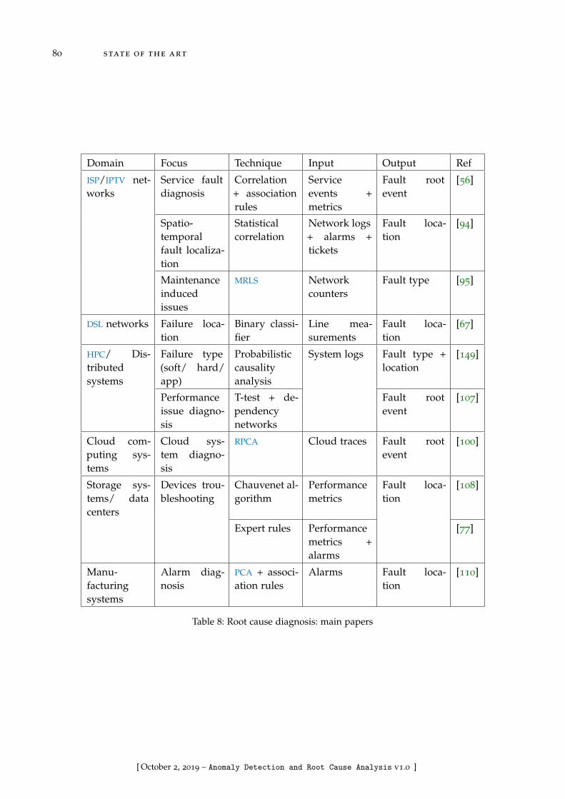
80 state of the art
Domain Focus Technique Input Output Ref
ISP/IPTV net-works
Service faultdiagnosis
Correlation+ associationrules
Serviceevents +metrics
Fault rootevent
[56]
Spatio-temporalfault localiza-tion
Statisticalcorrelation
Network logs+ alarms +tickets
Fault loca-tion
[94]
Maintenanceinducedissues
MRLS Networkcounters
Fault type [95]
DSL networks Failure loca-tion
Binary classi-fier
Line mea-surements
Fault loca-tion
[67]
HPC/ Dis-tributedsystems
Failure type(soft/ hard/app)
Probabilisticcausalityanalysis
System logs Fault type +location
[149]
Performanceissue diagno-sis
T-test + de-pendencynetworks
Fault rootevent
[107]
Cloud com-puting sys-tems
Cloud sys-tem diagno-sis
RPCA Cloud traces Fault rootevent
[100]
Storage sys-tems/ datacenters
Devices trou-bleshooting
Chauvenet al-gorithm
Performancemetrics
Fault loca-tion
[108]
Expert rules Performancemetrics +alarms
[77]
Manu-facturingsystems
Alarm diag-nosis
PCA + associ-ation rules
Alarms Fault loca-tion
[110]
Table 8: Root cause diagnosis: main papers
[ October 2, 2019 – Anomaly Detection and Root Cause Analysis v1.0 ]

8P R O P O S E D A L G O R I T H M : A R C D
8.1 introduction
Cellular networks have become more complex over the years, with multiple co-existingRadio Access Technologies (RATs) from 2G to 4G and now 5G, multiple core networkdevices from various vendors, multiple services that go beyond regular telephony, andmultiple handsets running various Operating Systems (OSs). This growing complexitymakes the task of monitoring the network and identifying the cause of performancedegradation more challenging for network operators [147]. Most devices in the networkgenerate log messages detailing their operations. Based on these messages it is possibleto reconstruct what happened in the network, at least to a certain extent. But, given thesheer number and variety of these messages, it is not feasible for human operators toanalyze all of them directly. This is why log messages are usually pre-processed beforebeing scrutinized by human experts who are in charge of identifying and mitigatingthe issues by appropriate actions. This analysis, while partly automated and aided byad-hoc tools [112], is often time consuming and inefficient. Network operators wouldlike to increase the automation of this analysis, in particular for cellular networks, inorder to reduce the time needed to detect, and fix, performance issues and to spot morecomplicated cases that are not always detected by human operators.
The data that are generated by the monitoring system are a large number of logentries (or simply logs), each of them being the report of what happened during a session.The term session depends on the specific service: Call Data Record (CDR) for a regularphone call or Session Data Record (SDR) for a service based on IP. The log takes usuallythe form of a series of 2-tuples (feature, value). The feature is a name indicating thenature of the corresponding value (for example cell identifier, content provider, handsetmanufacturer), while the value is what has been collected for this particular session (in
Cellular Network
Monitoring SystemCDR
SDR
MME
eNodeB SGW
eNodeB
PGW
PGWSGWInternet
TelephoneNetwork
ContentProvider
ContentProvider
Figure 38: System architecture of an LTE network with a subset of the monitored elements;eNodeB, PGW, SGW, and MME
81
[ October 2, 2019 – Anomaly Detection and Root Cause Analysis v1.0 ]

82 proposed algorithm : arcd
our example, a number that enables to uniquely identify the cell, the name of a provider,and the name of a manufacturer). The root cause of a network malfunction can be eithera certain 2-tuple, or a combination of k 2-tuples. Figure 38 shows a simplified view of anLTE cellular network, including some of its elements and the corresponding monitoringsystem, which collects data from the different devices to produce the CDRs and SDRs.
Despite an abundant literature related to network monitoring, identifying the rootcause of problems in modern cellular networks is still an open research question dueto specific requirements related to the nature of this type of networks [102]: First, adiagnosis system should work on various types of logs (voice calls, data sessions, multi-media sessions) because, nowadays, cellular networks carry significant amounts of datatraffic as well as voice. Second, a diagnosis solution has to deal with an increasing num-ber of features. Logs can now include features related to the service (e.g., the contentprovider, the quality and priority classes), to the network (e.g., the RAT and the gatewaysinvolved), and to the user (e.g., the handset type and the handset manufacturer). Fur-thermore, these features can depend on each other due to the architecture of networkand services. Third, a diagnosis solution has to address the complex interplay betweenfeatures, for example, an OS version not supporting a particular service. Both the serviceand the OS can behave normally in a majority of sessions when scrutinized indepen-dently; the issue can only be diagnosed in logs containing both. Finally, the diagnosissolution should focus on problems that have an actual impact on the network perfor-mance. A problem that happens sometimes in a device that is used by millions of userscan have a greater importance than a problem happening always in a device used by onlya few users. The balance between number of occurrences and inefficiency is a matter ofprioritizing mitigation actions.
Our goal is to design a diagnostic system, which addresses three key and challengingfeatures that network operator management teams are waiting for:
• Identifying Major Contributors: We call major contributors all the elements thatcause a significant decrease of the overall network efficiency. For example, a faultyMME results in the drop of a large number of calls. Our goal is to identify themajor contributors in the whole set of logs. Once these major contributors havebeen identified, it is possible for human experts to scrutinize them in order toresolve the underlying issues.
• Detecting Incompatibilities: A consequence of the great variety of devices in-volved is that incompatibilities between some of them can also result in poorQuality of Experience (QoE) for the users. An incompatibility is a failing combi-nation of two, otherwise properly working, elements. As previously stated, a newrelease of an OS can typically be incompatible with a service (e.g., voice calls, tollnumbers).
• Forming Equivalence Classes: Equivalence classes are sets of key-feature valuesthat correspond to the same underlying problem or that are strongly correlated.For instance, if a cell has only a few users and one of them is significantly moreactive than all the others (e.g., an automated bot making robocalls) and if thecorresponding International Mobile Subscriber Identity (IMSI) has an abnormallyhigh failure rate, the corresponding cell might have an abnormally high failure rate
[ October 2, 2019 – Anomaly Detection and Root Cause Analysis v1.0 ]
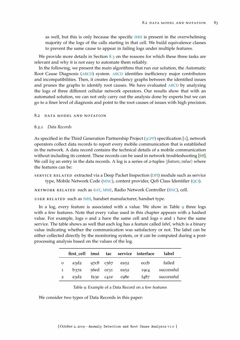
8.2 data model and notation 83
as well, but this is only because the specific IMSI is present in the overwhelmingmajority of the logs of the calls starting in that cell. We build equivalence classesto prevent the same cause to appear in failing logs under multiple features.
We provide more details in Section 8.3 on the reasons for which these three tasks arerelevant and why it is not easy to automate them reliably.
In the following, we present the main algorithms that run our solution, the AutomaticRoot Cause Diagnosis (ARCD) system. ARCD identifies inefficiency major contributorsand incompatibilities. Then, it creates dependency graphs between the identified issuesand prunes the graphs to identify root causes. We have evaluated ARCD by analyzingthe logs of three different cellular network operators. Our results show that with anautomated solution, we can not only carry out the analysis done by experts but we cango to a finer level of diagnosis and point to the root causes of issues with high precision.
8.2 data model and notation
8.2.1 Data Records
As specified in the Third Generation Partnership Project (3GPP) specification [1], networkoperators collect data records to report every mobile communication that is establishedin the network. A data record contains the technical details of a mobile communicationwithout including its content. These records can be used in network troubleshooting [68].We call log an entry in the data records. A log is a series of 2-tuples (feature, value) wherethe features can be:
service related extracted via a Deep Packet Inspection (DPI) module such as servicetype, Mobile Network Code (MNC), content provider, QoS Class Identifier (QCI).
network related such as RAT, MME, Radio Network Controller (RNC), cell.
user related such as IMSI, handset manufacturer, handset type.
In a log, every feature is associated with a value. We show in Table 9 three logswith a few features. Note that every value used in this chapter appears with a hashedvalue. For example, logs 0 and 2 have the same cell and logs 0 and 1 have the sameservice. The table shows as well that each log has a feature called label, which is a binaryvalue indicating whether the communication was satisfactory or not. The label can beeither collected directly by the monitoring system, or it can be computed during a post-processing analysis based on the values of the log.
first_cell imsi tac service interface label
0 a3d2 97c8 c567 ea52 eccb failed
1 b37a 56ed ce31 ea52 19c4 successful
2 a3d2 fa3e c41e c98e f487 successful
Table 9: Example of a Data Record on a few features
We consider two types of Data Records in this paper:
[ October 2, 2019 – Anomaly Detection and Root Cause Analysis v1.0 ]
84 proposed algorithm : arcd
CDR the records of voice calls. Each time a subscriber attempts to make a call, a CDR iscreated. If the call is dropped, the CDR is labeled as failed.
SDR the records created to track every Internet connection in cellular networks. AnSDR is created each time a subscriber attempts to use an online mobile applica-tion. SDRs are often the summary of multiple Transmission Control Protocol (TCP)connections initiated by the mobile application. Unlike CDRs, SDRs are not labeled.However, it is possible to estimate the QoE for the user and thus to attribute a label,based on the data rate, response time, and retransmission ratio.
Thanks to the success/fail label, it is possible to compute the network inefficiency, thatis the proportion of failed communications. This proportion can be computed over allthe logs, or it can be relative to a specific subset (e.g., all the logs that share a givenfeature-value pair).
8.2.2 Notation
Let E be a set of logs and f1, f2, ..fn be the features of the logs. A log x ∈ E can also berepresented as a vector x = (x1, x2, . . . , xn) where xi is the value of the feature fi. Sinceevery log has a label, we can partition E in two disjoint subsets: S containing the logslabelled as successful and F containing the logs labelled as unsatisfactory (i.e., failed).
We introduce the notion of signature to group the logs that have certain similarities.A k-signature s is the set of all logs, irrespective of their label, where k pre-determinedfeatures fp1 , fp2 , . . . , fpk (1 6 pi 6 n,∀i) have k specific values sp1 , sp2 , . . . , spk. Wecall the parameter k the order of the signature.
For instance, a 2-signature s that groups all logs from cell ab34 and a mobile phonerunning the OS b4e8 can be represented as:
((first cell, ab34) , (handset os, b4e8))
We denote by E(s) the set of all logs matching the signature s, regardless of their labels.Similarly, we denote by S(s) (respectively F(s)) the set of all successful (respectivelyfailed) logs matching signature s.
We define a few quantities that are useful to characterize signatures. (The operator |.|denotes the cardinality of a set.)
signature proportion (π): the proportion of logs matching s:
π(s) =|E(s)|
|E|
complementary signature proportion (π): the proportion of logs that do notmatch s:
π(s) = 1− π(s)
failure ratio (λ): the proportion of failed logs among those matching s:
λ(s) =|F(s)|
|E(s)|
[ October 2, 2019 – Anomaly Detection and Root Cause Analysis v1.0 ]
8.3 objectives of the diagnostic system 85
complementary failure ratio (λ): the proportion of failed logs in the data setwithout considering the logs matching s:
λ(s) =|F|− |F(s)|
|E|− |E(s)|
8.3 objectives of the diagnostic system
Modern cellular networks are complex systems, containing several devices of differenttypes. Network operators run extensive monitoring systems to keep a constant watchon all these devices, in order to detect misbehaving and faulty ones. Faulty devices arenot the only element to influence the QoE of the end-users. For instance, roaming userscould be prevented from accessing the network because a misconfiguration of an MME.Users often want to communicate with people (or services) hosted on networks otherthan the one of the cellular one they are connected to. Because of this, problems in othernetworks can result in a poor QoE for some of the users of a given cellular network.
8.3.1 Major Contributors
One of the consequences of the ever increasing usage of cellular networks is that, eventhough the overwhelming majority of users have an acceptable QoE, there is no shortageof failed logs in most production networks. Operators would like to be able to iden-tify as quickly as possible, and as efficiently as possible, the major contributors, that isthe feature-value pairs (or their combination) denoting elements causing a significantdecrease of the network efficiency.
Unfortunately one has to be careful when applying the definition of major contribu-tors, as it can lead to some undesirable results. First, because there is a inherent hierarchyin the cellular network, one can significantly increase the efficiency of the network by ex-cluding all the logs that share a very popular feature-value pair. For instance, we couldnotice a drastic increase of the efficiency after excluding the logs matching a device inthe core network. This does not necessarily mean that the core network element is de-ficient. If we have multiple user and cell issues, these issues combined may lead to ahigh failure ratio of the core network element. Thus, the core network element may bediagnosed as faulty whereas it functions correctly.
Second, some elements appear in a statistically significant number of logs, have a highfailure ratio, but their inefficiency is extrinsic, i.e., caused by other elements. For example,a Base Station Controller (BSC) connected to four cells can be involved in a large numberof calls. If two or three of its connected cells are faulty, excluding all the logs referencingthis BSC would result in a larger increase in the efficiency than excluding only the logscontaining one of the cells. But we are interested in identifying the faulty cells ratherthan the functioning BSC.
Third, some elements are highly inefficient (they fail often), however they do notappear in a large number of logs. For instance a subscriber can attempt to make a singlecall, which is dropped. The inefficiency of the IMSI of the subscriber is 1.0 however it iscalculated on only one log. This IMSI cannot be considered as a major contributor sinceits removal has no visible impact on the overall inefficiency. This example illustrates
[ October 2, 2019 – Anomaly Detection and Root Cause Analysis v1.0 ]
86 proposed algorithm : arcd
the tension between major contributors and weak signals, i.e., elements that have a highinefficiency but that are shared by a small number of logs.
8.3.2 Incompatibilities
While major contributors can potentially affect a non-negligible number of users, incom-patibilities often affect fewer users, making them a less urgent issue. For example, eventhough voice calls using a given technology (4G or 2G) have a very low failure rate,calls started with 4G and then switched to 2G may have an abnormally high failure rate.The reason behind this incompatibility may be an incorrect configuration of the CircuitSwitched Fallback (CSFB) procedure or the use of devices from different vendors. Simi-larly, a new release of a smart phone OS could not be compatible with the Tranport LayerSecurity (TLS) implementation used by a certain content provider, because of a bug inthe implementation of the TLS handshake in the new release.
ARCD detects as incompatibilities all the cases where a combination of two otherwiseworking elements results in a higher failure rate. Certain cases that fall within this cat-egory do not necessarily conform with the definition of the term “incompatibility.” Forexample, consider two neighboring cells that work correctly but such that there is apoorly covered area between the two, so that all the calls started in one cell and thenhanded over to the other experience a high drop rate. ARCD detects this as an incompat-ibility, even though, there are no two incompatible devices here. This is, nonetheless, anissue that must be detected and addressed in order to increase customer satisfaction.
It is extremely hard for human operators to detect incompatibilities simply by look-ing at the logs, unless these affect a significant number of logs. This is why networkoperators need automated solutions that can identify them with little or no human in-tervention. As we discuss in Section 8.6.5.3, detecting incompatibilities is more compu-tationally intensive than detecting major contributors, this is why ARCD addresses eachproblem separately, giving operators the freedom to decide how often to trigger eachoperation.
8.3.3 Equivalence Classes
ARCD detects both types of anomaly (major contributors and incompatibilities) as a setof one, or more, feature-value pair(s). Because logs are meant to accurately represent thewidest possible number of cases, they contain between 30 and 60 different features (seeTable 10 for the precise number of features present in each data set). It is common to seea strong correlation between one or more features for a set of logs. For example, all SDR
corresponding to a given service (feature service provider) can have the same value for theIP address of the service (feature host), whenever the service provider exposes a singleIP address as it does happen for smaller service providers. In this specific example, thereis a perfect correlation between the two features, making them completely equivalent fora subset of the logs.
The correlation can also reflect the hierarchy of the cellular network. In the examplementioned above, about a single failing IMSI in a cell with few users, the IMSI feature
[ October 2, 2019 – Anomaly Detection and Root Cause Analysis v1.0 ]

8.4 major contributor detection 87
is not exactly equivalent to the cell-id feature, but, for the purpose of identifying theunderlying problem, they are indeed equivalent.
It is important for ARCD to be able to detect these equivalence classes automatically,in order to present them to the human operators, who could otherwise be overwhelmedby a long unorganized list of feature-value pairs. This is why we build a directed graphwhere each node contains one or more feature value pair. Such a data structure has theadded advantage of being well suited to build interactive visualizations allowing usersto easily navigate between the different problems and to drill down into the details ofeach one when needed.
8.4 major contributor detection
We now explain how ARCD processes data records to detect major contributors and howit then filters the results to produce a graph of dependencies between issues occurringin the network. The first step is to label each log as successful or failed if the inputlogs are not already labeled. Then, it identifies the top signatures responsible for thenetwork inefficiency. These signatures are then classified into equivalence classes, whichare groups of signatures corresponding to the same problem. Then it generates a graphoutlining the dependencies between all the problems. It finishes by pruning the graph toremove unnecessary nodes denoting false problems (elements appearing as inefficientbecause they share a part of their logs with malfunctioning ones). Figure 39 gives agraphical representation of these steps, which are detailed below.
MonitoringSystem
LabelingSDRs Top Sig-natures
Detection
LabelledSDRs
CDRs
EquivalenceClass Com-
putation
Top
Signatures
GraphCompu-tation
IssueClasses
GraphPruning
IssueDependencies
PrunedGraph
Figure 39: Major contributor detection steps
8.4.1 Labeling
The first step consists in labeling the logs. If the data has no success/failure label, wecreate a binary feature based on standardized criteria specified by the 3GPP. In the caseof CDRs, we have a label success/failure based on the Session Initiation Protocol (SIP)messages exchanged between network devices. In the case of SDRs, we assess the Qualityof Service (QoS) of TCP connections based on metrics such as mobile response time, serverresponse time and re-transmission ratio. For each metric, we set a lower bound for anacceptable QoS. An SDR with one value below the threshold is labeled as failed.
[ October 2, 2019 – Anomaly Detection and Root Cause Analysis v1.0 ]

88 proposed algorithm : arcd
8.4.2 Top Signature Detection
The second step consists in identifying the top 1-signatures contributing to the overallinefficiency of the network. To do so, we start by generating the set of all 1-signatures,that is the set of all possible values taken by each one of the features. Then, for eachsignature we compute two values: the Complementary Signature Proportion π and theComplementary Failure Ratio λ. The 1-signatures with the smallest values of λ corre-spond to the major contributors: removing all the logs belonging to these signaturesresults in smallest overall failure ratio for the remaining logs. Some of these signaturesmatch a significant fraction of the logs in the system, for instance because the 1-signaturecorresponds to a device that handles a lot of traffic with a slightly higher failure ratiothan the rest of the network.
There is a trade-off between inefficiency and representativeness. The ComplementarySignature Proportion (π) indicates whether a 1-signature matters. The larger is π(s), theless common is the signature s. Our trade-off is thus as follows: on the one hand wewant signatures with the smallest values of λ but not if the corresponding π is too small.We achieve this goal by maximizing a linear combination of these two values:
ν(s) = π(s) −αλ(s)
where α is a parameter to weigh the two aspects mentioned above. For small valuesof α, the dominant term of the score ν is π. Thus, the signatures with the highest νwill be signatures with few matching logs and a relatively high failure ratio. This way,we highlight "weak signals". However, for large values of α, the dominant term of ν isαλ. In this case, the signatures with high ν will be signatures having large impact onthe overall failure ratio in the network. These signatures generally match a large set oflogs and are consequently called "major contributors". To have a robust solution, we useseveral values of α: ten values between 0 and 1 (0.1, 0.2, 0.3, . . . , 0.9) and then twentyvalues between 1 and 20 (1, 2, 3, . . . , 20). The first set of values (α < 1) corresponds to theweak signals while the second corresponds to the major contributors.
For each one of these values of α, we compute ν for each 1-signature and we take thetwenty signatures with the largest values of ν (“top twenty”). We then compute howmany times one of these signatures is in a top twenty. A signature that appears oftenin the top twenty corresponds to a potential problem. In all our data sets, it is indeedthe case that several signatures appear multiple times in the different top twenties. Wecomplete this step by taking the fifty signatures that appear more often in the top twenty.However, we cannot stop here because some of these 1-signatures could correspond tothe same underlying problem. That is what the following step addresses.
8.4.3 Equivalence Class Computation
This step consists in grouping signatures related to the same problem. As an example,consider a user connecting to a cell, where he is the only active user, with an uncommonhandset type. If, for some reason, the user experiences many consecutive bad sessions,the resulting logs are labeled as failed. In this case, the corresponding IMSI, handsettype, and the cell-id appear at the top of the signature list that we generated in theprevious step. The three signatures point to the same problem rather than three separate
[ October 2, 2019 – Anomaly Detection and Root Cause Analysis v1.0 ]
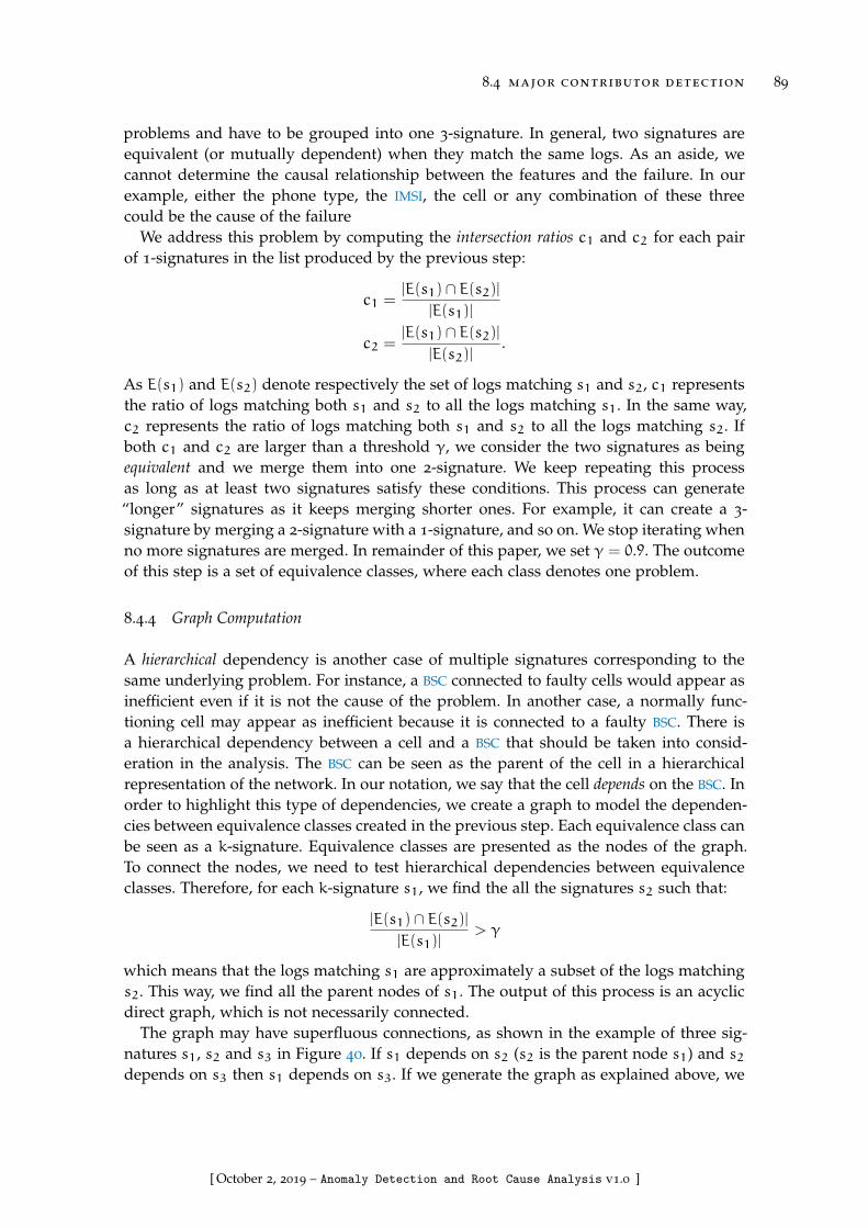
8.4 major contributor detection 89
problems and have to be grouped into one 3-signature. In general, two signatures areequivalent (or mutually dependent) when they match the same logs. As an aside, wecannot determine the causal relationship between the features and the failure. In ourexample, either the phone type, the IMSI, the cell or any combination of these threecould be the cause of the failure
We address this problem by computing the intersection ratios c1 and c2 for each pairof 1-signatures in the list produced by the previous step:
c1 =|E(s1)∩ E(s2)|
|E(s1)|
c2 =|E(s1)∩ E(s2)|
|E(s2)|.
As E(s1) and E(s2) denote respectively the set of logs matching s1 and s2, c1 representsthe ratio of logs matching both s1 and s2 to all the logs matching s1. In the same way,c2 represents the ratio of logs matching both s1 and s2 to all the logs matching s2. Ifboth c1 and c2 are larger than a threshold γ, we consider the two signatures as beingequivalent and we merge them into one 2-signature. We keep repeating this processas long as at least two signatures satisfy these conditions. This process can generate“longer” signatures as it keeps merging shorter ones. For example, it can create a 3-signature by merging a 2-signature with a 1-signature, and so on. We stop iterating whenno more signatures are merged. In remainder of this paper, we set γ = 0.9. The outcomeof this step is a set of equivalence classes, where each class denotes one problem.
8.4.4 Graph Computation
A hierarchical dependency is another case of multiple signatures corresponding to thesame underlying problem. For instance, a BSC connected to faulty cells would appear asinefficient even if it is not the cause of the problem. In another case, a normally func-tioning cell may appear as inefficient because it is connected to a faulty BSC. There isa hierarchical dependency between a cell and a BSC that should be taken into consid-eration in the analysis. The BSC can be seen as the parent of the cell in a hierarchicalrepresentation of the network. In our notation, we say that the cell depends on the BSC. Inorder to highlight this type of dependencies, we create a graph to model the dependen-cies between equivalence classes created in the previous step. Each equivalence class canbe seen as a k-signature. Equivalence classes are presented as the nodes of the graph.To connect the nodes, we need to test hierarchical dependencies between equivalenceclasses. Therefore, for each k-signature s1, we find the all the signatures s2 such that:
|E(s1)∩ E(s2)||E(s1)|
> γ
which means that the logs matching s1 are approximately a subset of the logs matchings2. This way, we find all the parent nodes of s1. The output of this process is an acyclicdirect graph, which is not necessarily connected.
The graph may have superfluous connections, as shown in the example of three sig-natures s1, s2 and s3 in Figure 40. If s1 depends on s2 (s2 is the parent node s1) and s2depends on s3 then s1 depends on s3. If we generate the graph as explained above, we
[ October 2, 2019 – Anomaly Detection and Root Cause Analysis v1.0 ]
90 proposed algorithm : arcd
S3
S2
S1
Case 1
S4
S5S6
S7
Case 2
Figure 40: Examples of multiple paths between nodes containing signatures
have two paths between s1 and s3: a direct connection and another connection via s2.In this case, the direct connection between s1 and s3 is irrelevant since it does not addany information compared to the connection via s2. To solve this problem, we use theDepth-first Search algorithm to find all the paths between every pair of connected nodesand then we keep only the longest path. Keeping only the longest path does not lead toany information loss.
Consider the second case in Figure 40. There are three paths from s4 to s7. Withoutloss of generality, assume that we have considered the path through s6 as the longestone. Then, we will keep only this path between s4 and s7. But, since s4 depends ons5 (and there is only one path between s4 and s5), this link is kept as the longest onebetween s4 and s5. The same argument applies to the link between s5 and s7. In thiscase we end up removing only the direct link between s4 and s7.
8.4.5 Graph Pruning
The structure of the graph allows the exploration of faulty devices and services in ahierarchical way: At the top, we find frequent signature (having a high π) such as corenetwork equipment, popular services and handset manufacturers. At the bottom of thegraph, we have less frequent signatures such as user IMSIs, host IP addresses, and theleast used cell-ids.
In a well-constructed graph, we need each child node to have extra information com-pared to its parent nodes. Otherwise, it is irrelevant and it should be removed. In ourcase, we know that the parent node is inefficient to some extent (all the nodes in thegraph are made up of the inefficient signatures selected in step 1). And, as the childnode matches a subset of logs of the parent, it is expected to be inefficient as well. There-fore, presenting the child node is meaningful only in the case where it is more inefficientthan at least one of its parent nodes. To remove superfluous nodes, we define a measurecalled Relative Failure Ratio λr. Suppose that we have two connected nodes (parent andchild). λr is defined as follows:
λr(sc, sp) =λ(sc) − λ(sp)
λ(sp)
where sp is the signature in the parent node and sc the one in the child node. Foreach node, we calculate its relative failure ratio with respect to all its parents. We keepthe node if at least one of the relative failure ratios is greater than 0.01. Otherwise, we
[ October 2, 2019 – Anomaly Detection and Root Cause Analysis v1.0 ]

8.4 major contributor detection 91
cell12cf
mncaf1e
imsib513
imsi9f56
imsi32ac
imsidaa3
imsi5e5a
Figure 41: Pruning Scenario
remove it. Every time we remove a node, we connect its ancestors with its successors.After this pruning operation, every child node in the graph is more inefficient than atleast one of its parent nodes. In such case, we have two possible scenarios:
• In the first one, the child node presents a separate problem. This could be the caseof a user trying continuously to call an unreachable number through a cell havingan interference problem. In the graph, we can find the node containing the userIMSI as a child of cell-id node with user IMSI failure ratio being higher than the cellfailure ratio. The user calling an unreachable number and the radio interferenceproblem are two separate issues. It is therefore important to keep the two nodes.
• In the second one, the child node is the root of the inefficiency of the parent node.Figure 41 illustrates an example of this scenario. Consider the case of a large groupof roaming users (tourists, for example) accessing the network through a small cell(with few resident users). In Figure 41, the id of the small cell is 12cf. The MNC ofthe home network of the roaming users is af1e. There is a resident user with anIMSI b513 and four roaming users whose IMSIs are 9f56, 32ac, daa3, and 5e5a. Theroaming users may experience a bad QoE because of a roaming issue between theirhome network and the host network. Since the roaming users are the main usersof the cell, the cell has a high failure ratio λ. In the graph, we find the MNC of theroaming users as a child node of the cell. The MNC may have a slightly higher λcompared to the cell. In this case, the node containing the cell-id has to be removedsince roaming is the real issue.
To deal with the second scenario, we proceed as follows. Consider two connectednodes: a parent node sp and a child node sc. Let λn be the overall failure ratio of thenetwork.
λn =|F|
|E|
Our goal is to know whether the high failure ratio of sp is due to sc. To do so, werestrict to the logs matching sp, E(sp) instead of using the whole data set. In this subsetwe calculate the complementary failure ratio λ(sc) which is the failure ratio of sp afterremoving the logs matching sc. If λ(sc) 6 λn, then sp is a non faulty signature andthe parent node is removed. Otherwise, we are in the first scenario and the two nodes
[ October 2, 2019 – Anomaly Detection and Root Cause Analysis v1.0 ]

92 proposed algorithm : arcd
present two different problems. As previously mentioned, each time we remove a node,we connect its ancestors to its successors. With these new connections, we may haveother nodes to remove. We repeat the pruning process as long as it has removed at leastone node in the previous iteration. This process is guaranteed to terminate as it onlyremoves nodes.
8.5 incompatibility detection
The procedure described in Section 8.4 allows us to detect major contributors that havea high impact on the network inefficiency. In this section, we explain how ARCD findsincompatibilities. By definition, these involve more than one feature-value pair makingtheir detection more computationally demanding than major contributors. For the latter,we only needed to compute all the 1-signatures, that is the set of all logs having thesame feature-value pair, for all the different feature-value pair present in the logs. Whenlooking for incompatibilities, we compute all the 2-signatures that is the set of all logshaving the same two feature-values for two features, for all the features and their valuesin the logs. Because of this, finding incompatibilities requires more memory and moreprocessing time. We decided to separate the two problems so that operators can decidewhen to trigger each detection separately, depending on their needs and the availabilityof computing resources.
MonitoringSystem
LabelingSDRs DetectingIncom-
patibilitySignatures
LabelledSDRs
CDRs
FilteringFalse Incom-patibilities
Incompatible
Signatures
1-signatures
EquivalenceClass Com-
putation
Incompatible
Signatures
GraphCompu-tation
Issue Classes
GraphPruning
IssueDependencies
PrunedGraph
Figure 42: Incompatibility detection steps
Figure 42 describes the main steps of incompatibility detection. We start by labelingdata as explained in Section 8.4.1. Then we identify the signatures pointing to incom-patibilities throughout the network. Next, we filter false incompatibilities, that is caseswhere the inefficiency in the logs sharing a given 2-signature is actually explained by athird faulty element that is also present in most of the logs of the 2-signature in question.Finally, similarly to Section 8.4, we compute the equivalence classes.
[ October 2, 2019 – Anomaly Detection and Root Cause Analysis v1.0 ]

8.5 incompatibility detection 93
8.5.1 Identifying incompatible signatures
The goal of this step is to find the signatures corresponding to incompatible elements.To do so, we start by generating the sets of all 1-signatures and 2-signatures. For eachsignature, we measure the failure ratio λ. To decide whether a 2-signature points anincompatibility, we proceed as follows.
Let us consider a 2-signature s = fi = vi, fj = vj where vi and vj are values taken bythe features fi and fj, corresponding to two 1-signatures (si = fi = vi and sj = fj = vj
respectively). For example, we could have:
si = (service, a587) sj = (handset os, c255)
s = ((service, a587), (handset os, c255)).
To determine whether two feature-value pairs are incompatible, we compute the gainof s, defined as:
g(s) = λ(s) − max(λ(si), λ(sj)).
The gain allows us to evaluate the impact of combining two 1-signatures on the failureratio. In other words, we check if the combination of two elements is more inefficientthan each one apart. If the gain is larger than a threshold, set to 0.2 in our implementa-tion, we consider that the 2-signature s corresponds to incompatible elements.
8.5.2 Filtering False Incompatibilities
A combination with a higher failure ratio than each of its components does not implyautomatically that we are dealing with an incompatibility. For example, consider theservice type Instant Messaging (IM) and a specific content provider, both having a lowfailure rate. However, the combination of these two elements has a high failure rate. Thiscombination could be identified in the previous step as an incompatibility. However, bystudying the logs matching this combination, we may find a single host delivering IM
service in the content provider network. The root of the issue, here, is not an incompati-bility between IM and the content provider but rather a malfunctioning host.
In order to filter such cases, we proceed as follows. For each 2-signature selected inthe previous step (s), we identify its matching set of logs E(s). In this subset, we find allthe 1-signatures t that represent a significant fraction of E(s):
τ(s) =
t||E(t)∩ E(s)|
|E(s)|> γ
where γ = 0.9. Then, we re-compute the gain:
g(s) = λ(s) − maxt∈τ
(λ(t)).
If the gain remains higher than the threshold (0.2), it means that the combination isa real incompatibility: There is no third element with a high failure ratio co-occurringwith the combination. Otherwise, if the gain drops below the threshold, there is a thirdelement that is at the origin of the high failure ratio rather than the combination of thetwo elements. In this case, the issue is not an incompatibility but a highly inefficientsingle element. We report this element separately with the appropriate 1-signature andwe discard the corresponding 2-signature from the incompatibility list.
[ October 2, 2019 – Anomaly Detection and Root Cause Analysis v1.0 ]

94 proposed algorithm : arcd
8.5.3 Equivalence Class Computation
At this point, we have a list of 2-signatures corresponding to incompatibilities. But someof the signatures might actually correspond to the same underlying issue. For instance,suppose that we detected an incompatibility between a handset type and an eNodeB
identifier. Suppose as well that this eNodeB has only one static IP address so that wecould have detected the same incompatibility twice. In this case we should group theeNodeB identifier and its IP address as an equivalence class that is incompatible with thehandset type. The goal of this step is to find for each feature-value pair present in oneof the 2-signatures, the classes of elements that are incompatible with it.
Let Ω be the set of all 2-signatures that have passed the filtering step, where each 2-signature (ωi) is composed of two 1-signatures βi, δi. For each one of these constituent1-signatures we build a list of all the other 1-signatures with which it is incompatible.In other words, for every 1-signature (ρ) in the union of all the βi and δi we computeI(ρ) = θ|(ρ, θ) ∈ Ω or (θ, ρ) ∈ Ω. As I(ρ) is a set of 1-signatures, we can proceed as inSection 8.4.3 to group I(ρ) into equivalence classes. Recall that this process can create“longer” signatures (2-signatures, 3-signatures, etc.) so that, at the end of this process,for each 1-signature ρ, which was in one of the original 2-signatures in Ω, we have a setof k-signatures that are incompatible with it.
8.5.4 Graph Computation
Some incompatibilities may result from other ones. For example, if a a service and an OS
are incompatible, all the OS versions will be incompatible with that same service. That iswhy, to identify the root incompatibility, we need to explore hierarchical dependencies.Therefore, for each signature ρ we use the equivalence classes computed in the previousstep to create a graph as we did in Section 8.4.4. Note that we have 2|Ω| graphs, that isa graph for each 1-signature ρ. This graph contains the signatures incompatible with ρgrouped into equivalence classes and connected based on their hierarchical dependen-cies.
8.5.5 Pruning
At this point of the analysis, for each 1-signature ρ, we have a graph of the elementsincompatible with ρ. For each pair of connected nodes in this graph, either the parent(θp) is the origin of the incompatibility with ρ or the child (θc) is the origin. We proceedas in Section 8.4.5 to distinguish between the two cases substituting the failure ratio λwith the gain g. In other words, we check if θp (the parent of θc) remains incompatiblewith ρ after removing the logs matching the child (θc): we remove the logs matching θc;then, we compute the gain of the incompatibility between θp and ρ. If the gain is higherthan the threshold, this means that the parent θp is incompatible with ρ independentlyof the child θc. The incompatibility of the child θc with ρ could be seen as a result(inheritance) of the incompatibility of the parent θp with ρ. In this case, we removeθc from the graph. If, on the contrary, the gain drops below the threshold, this meansthat the child θc is the origin of the incompatibility with ρ. As the logs of the child θc
[ October 2, 2019 – Anomaly Detection and Root Cause Analysis v1.0 ]

8.6 evaluation 95
Figure 43: System Architecture
are a subset of the logs of the parent θp, θp appeared as incompatible with ρ. In thiscase, we remove θp from the graph. Every time a node is removed, its ancestors areconnected to its successors. We iterate the pruning until we have only isolated nodes,which correspond to the signatures incompatible with ρ. Note that we execute the wholeprocess for each one of the constituent 1-signatures identified in the previous step.
8.6 evaluation
We have implemented ARCD in a Big Data cluster and ran major contributor detectionand incompatibility detection as Spark jobs scheduled by the task manager OAR asshown in Figure 43. The results are displayed in a Graphical User Interface (GUI). Weevaluate the effectiveness and performance of ARCD thanks to three different data sets,collected via Hadoop Distributed File System (HDFS) from three different live cellular net-works. After briefly presenting each data set, we analyze the major contributor detectionresults followed by the incompatibilities results. Finally, we compare the performance ofARCD with Learning from Examples Module, version 2 (LEM2), which is a well knownalgorithm for deducting decision rules from data.
8.6.1 Data Sets
We ran ARCD on three data sets from three different operators. The values of the featuresin the logs are anonymized by a hashing algorithm.
set 1 : SDRs recording TCP connections during one hour in a European country. A hu-man expert has cleaned and analyzed this data set so that we can use it as a refer-ence in the validation process. She removed samples with missing and inconsistentfields and truncated extreme values.
set 2 : SDRs recording TCP connections during one day from another European oper-ator. This set is a raw one (missing values, inconsistent values). This set was notexamined by an expert.
[ October 2, 2019 – Anomaly Detection and Root Cause Analysis v1.0 ]

96 proposed algorithm : arcd
set 3 : CDRs logging voice calls during one day from an Asian operator. This is also araw data set with no pre-specified root causes but where each entry is labeled assuccessful/failed.
Table 10 summarizes some of the attributes of the data sets. We used the re-transmissionratio to label each entry for Set 1 and the server response time for Set 2. These metricswere suggested by the experts working with the corresponding operators.
set number number of number of failure
of logs features 1-signatures ratio
1 25 000 48 64 143 0.05
2 10 000 000 31 924 836 0.18
3 1 000 000 35 162 603 0.08
Table 10: Validation Data Sets
8.6.2 Expert Validation
We worked with three experts having more than ten years of experience in the domain ofmobile network troubleshooting. These experts helped us by providing feedback on theresults of our solution. They confirmed that ARCD extracts from the logs actionable infor-mation for network troubleshooting. They also appreciated the output being presentedas graphs that are straightforward to understand, greatly simplifying and streamliningthe analysis of the underlying issues and the planning of the mitigation actions.
8.6.3 Major Contributor Detection
To validate our results on Set 1, we compared the outcome of our solution with thelist of issues identified by human experts. To validate our results on Sets 2 and 3, wehave created an expert emulator, which mimics the manual analysis done by humanexperts. The emulator analyses a limited number of features (less than ten). For Sets 2
and 3, the experts supervising the networks of the corresponding operators have kindlyindicated the features they are focusing on. For each feature, the emulator scans the topten frequent elements (e.g., top popular services). If one element is more inefficient thanthe global network, the elements is identified as a major contributor. To pinpoint inef-ficient elements, the expert emulator calculates the following metrics for each elementand compares them to the the values of the whole network: failure ratio for CDRs (Set 3);Retransmission ratio (Set1) and server response time (Set 2). These metrics are the samewe used in the data labeling phase of ARCD. The concept of hierarchical dependenciesis implicitly included in the expert analysis: Experts start with high level elements (e.g.,devices in the core network) and then move down to lower levels (e.g., users).
[ October 2, 2019 – Anomaly Detection and Root Cause Analysis v1.0 ]
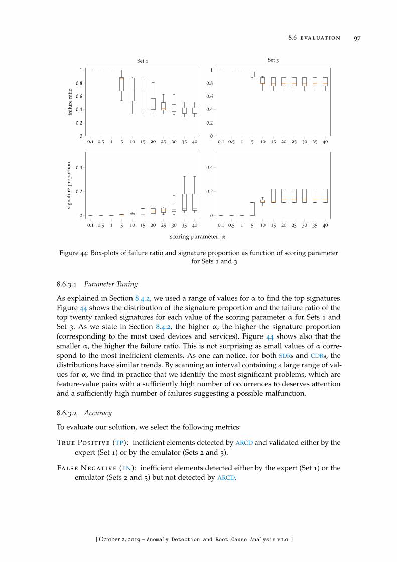
8.6 evaluation 97
0.1 0.5 1 5 10 15 20 25 30 35 40
0
0.2
0.4
0.6
0.8
1fa
ilure
rati
o
Set 1
0.1 0.5 1 5 10 15 20 25 30 35 40
0
0.2
0.4
0.6
0.8
1
Set 3
0.1 0.5 1 5 10 15 20 25 30 35 40
0
0.2
0.4
sign
atur
epr
opor
tion
0.1 0.5 1 5 10 15 20 25 30 35 40
0
0.2
0.4
scoring parameter: α
Figure 44: Box-plots of failure ratio and signature proportion as function of scoring parameterfor Sets 1 and 3
8.6.3.1 Parameter Tuning
As explained in Section 8.4.2, we used a range of values for α to find the top signatures.Figure 44 shows the distribution of the signature proportion and the failure ratio of thetop twenty ranked signatures for each value of the scoring parameter α for Sets 1 andSet 3. As we state in Section 8.4.2, the higher α, the higher the signature proportion(corresponding to the most used devices and services). Figure 44 shows also that thesmaller α, the higher the failure ratio. This is not surprising as small values of α corre-spond to the most inefficient elements. As one can notice, for both SDRs and CDRs, thedistributions have similar trends. By scanning an interval containing a large range of val-ues for α, we find in practice that we identify the most significant problems, which arefeature-value pairs with a sufficiently high number of occurrences to deserves attentionand a sufficiently high number of failures suggesting a possible malfunction.
8.6.3.2 Accuracy
To evaluate our solution, we select the following metrics:
True Positive (TP): inefficient elements detected by ARCD and validated either by theexpert (Set 1) or by the emulator (Sets 2 and 3).
False Negative (FN): inefficient elements detected either by the expert (Set 1) or theemulator (Sets 2 and 3) but not detected by ARCD.
[ October 2, 2019 – Anomaly Detection and Root Cause Analysis v1.0 ]
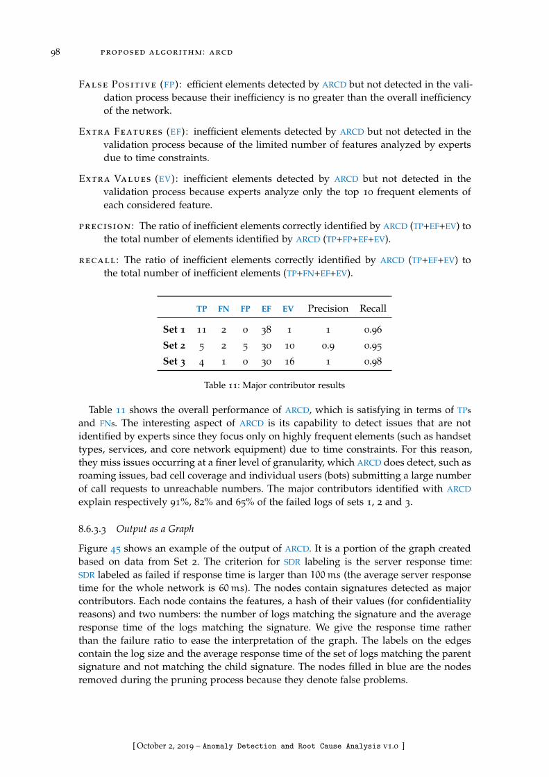
98 proposed algorithm : arcd
False Positive (FP): efficient elements detected by ARCD but not detected in the vali-dation process because their inefficiency is no greater than the overall inefficiencyof the network.
Extra Features (EF): inefficient elements detected by ARCD but not detected in thevalidation process because of the limited number of features analyzed by expertsdue to time constraints.
Extra Values (EV): inefficient elements detected by ARCD but not detected in thevalidation process because experts analyze only the top 10 frequent elements ofeach considered feature.
precision : The ratio of inefficient elements correctly identified by ARCD (TP+EF+EV) tothe total number of elements identified by ARCD (TP+FP+EF+EV).
recall : The ratio of inefficient elements correctly identified by ARCD (TP+EF+EV) tothe total number of inefficient elements (TP+FN+EF+EV).
TP FN FP EF EV Precision Recall
Set 1 11 2 0 38 1 1 0.96
Set 2 5 2 5 30 10 0.9 0.95
Set 3 4 1 0 30 16 1 0.98
Table 11: Major contributor results
Table 11 shows the overall performance of ARCD, which is satisfying in terms of TPs
and FNs. The interesting aspect of ARCD is its capability to detect issues that are notidentified by experts since they focus only on highly frequent elements (such as handsettypes, services, and core network equipment) due to time constraints. For this reason,they miss issues occurring at a finer level of granularity, which ARCD does detect, such asroaming issues, bad cell coverage and individual users (bots) submitting a large numberof call requests to unreachable numbers. The major contributors identified with ARCD
explain respectively 91%, 82% and 65% of the failed logs of sets 1, 2 and 3.
8.6.3.3 Output as a Graph
Figure 45 shows an example of the output of ARCD. It is a portion of the graph createdbased on data from Set 2. The criterion for SDR labeling is the server response time:SDR labeled as failed if response time is larger than 100ms (the average server responsetime for the whole network is 60ms). The nodes contain signatures detected as majorcontributors. Each node contains the features, a hash of their values (for confidentialityreasons) and two numbers: the number of logs matching the signature and the averageresponse time of the logs matching the signature. We give the response time ratherthan the failure ratio to ease the interpretation of the graph. The labels on the edgescontain the log size and the average response time of the set of logs matching the parentsignature and not matching the child signature. The nodes filled in blue are the nodesremoved during the pruning process because they denote false problems.
[ October 2, 2019 – Anomaly Detection and Root Cause Analysis v1.0 ]

8.6 evaluation 99
mnc:
c81e
8126762
.1mn
c:c4
ca324120.83
host:
2cc4
conte
nt_pr
ovide
r:7fe1
819119.76
conte
nt_ca
tegor
y:795f
servic
e:ea
52
3598972
.83diff:5189554
.17
host:
a3d2
3978069
.49
diff:4787455
.51
hand
set_m
anufa
cturer
:c291
225242.21
conte
nt_pr
ovide
r:d2ed
5819
80.71
diff:3103470
.23
host:
7cb
2
58308.66
diff:3593172
.45ser
vice:
627c
servic
e_typ
e:8818
4140
133.58
diff:3564062
.04
hand
set_ty
pe:3
352
tac:c
3a5
61645.7dif
f:164
92.13
diff:3972168
.6
host:
a59c
1916
129.26
diff:390356
.88
Figu
re4
5:P
rune
dG
raph
ofM
ajor
Con
trib
utor
sfo
rSe
t2
,nod
esin
blue
are
rem
oved
duri
ngth
epr
unin
gpr
oces
s
[ October 2, 2019 – Anomaly Detection and Root Cause Analysis v1.0 ]
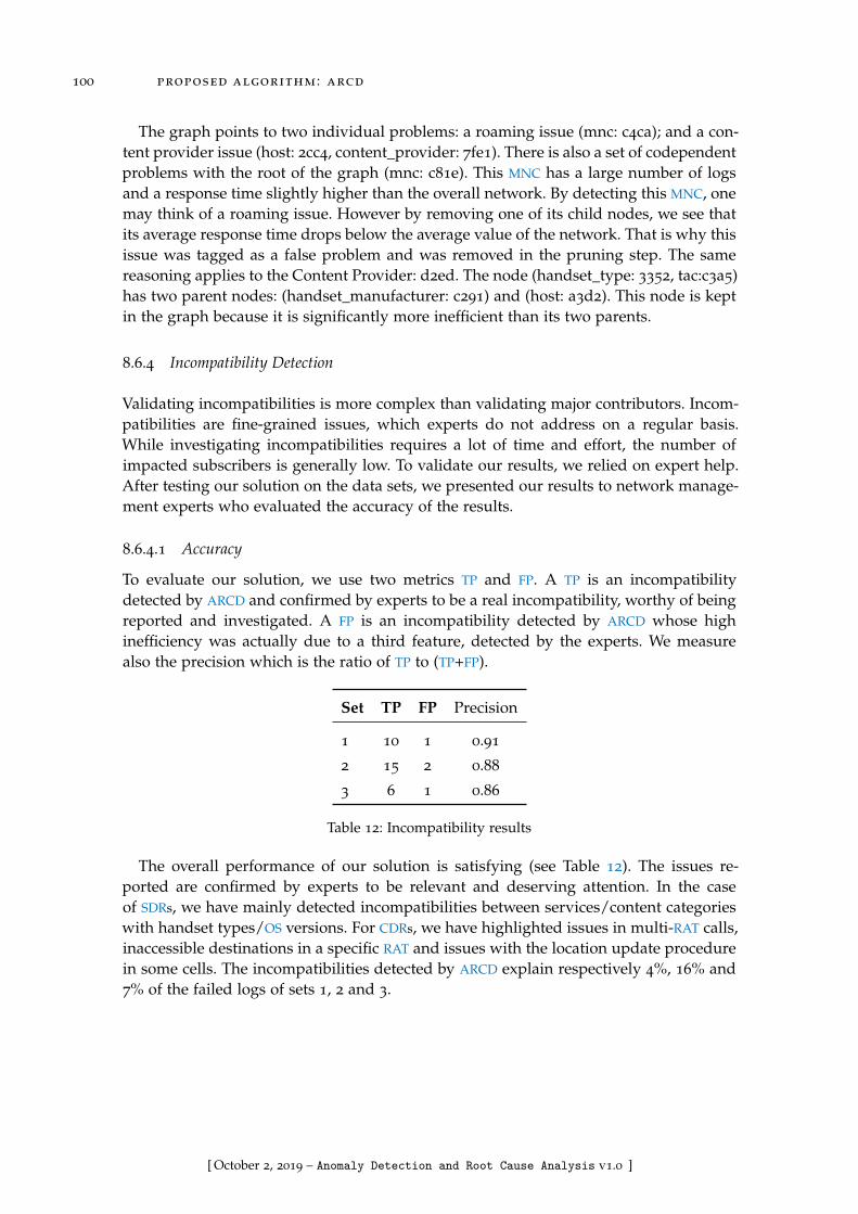
100 proposed algorithm : arcd
The graph points to two individual problems: a roaming issue (mnc: c4ca); and a con-tent provider issue (host: 2cc4, content_provider: 7fe1). There is also a set of codependentproblems with the root of the graph (mnc: c81e). This MNC has a large number of logsand a response time slightly higher than the overall network. By detecting this MNC, onemay think of a roaming issue. However by removing one of its child nodes, we see thatits average response time drops below the average value of the network. That is why thisissue was tagged as a false problem and was removed in the pruning step. The samereasoning applies to the Content Provider: d2ed. The node (handset_type: 3352, tac:c3a5)has two parent nodes: (handset_manufacturer: c291) and (host: a3d2). This node is keptin the graph because it is significantly more inefficient than its two parents.
8.6.4 Incompatibility Detection
Validating incompatibilities is more complex than validating major contributors. Incom-patibilities are fine-grained issues, which experts do not address on a regular basis.While investigating incompatibilities requires a lot of time and effort, the number ofimpacted subscribers is generally low. To validate our results, we relied on expert help.After testing our solution on the data sets, we presented our results to network manage-ment experts who evaluated the accuracy of the results.
8.6.4.1 Accuracy
To evaluate our solution, we use two metrics TP and FP. A TP is an incompatibilitydetected by ARCD and confirmed by experts to be a real incompatibility, worthy of beingreported and investigated. A FP is an incompatibility detected by ARCD whose highinefficiency was actually due to a third feature, detected by the experts. We measurealso the precision which is the ratio of TP to (TP+FP).
Set TP FP Precision
1 10 1 0.91
2 15 2 0.88
3 6 1 0.86
Table 12: Incompatibility results
The overall performance of our solution is satisfying (see Table 12). The issues re-ported are confirmed by experts to be relevant and deserving attention. In the caseof SDRs, we have mainly detected incompatibilities between services/content categorieswith handset types/OS versions. For CDRs, we have highlighted issues in multi-RAT calls,inaccessible destinations in a specific RAT and issues with the location update procedurein some cells. The incompatibilities detected by ARCD explain respectively 4%, 16% and7% of the failed logs of sets 1, 2 and 3.
[ October 2, 2019 – Anomaly Detection and Root Cause Analysis v1.0 ]

8.6 evaluation 101
hand
set_m
anufa
cturer
70d1
hand
set_ty
pe275a
tac 5941
tac918a
hand
set_ty
pe50ac
hand
set_ty
pe2f10 tac 6e26
hand
set_ty
pe3636
hand
set_ty
pe31aa
tac 831c
tac 11aa
hand
set_m
anufa
cturer
1fe4
tac3afb
hand
set_ty
pe27f4
hand
set_ty
pe15f7
taca8
93
Figu
re4
6:I
ncom
pati
bilit
ies
prun
edgr
aph
ofth
e1
-sig
natu
re(c
onte
nt_c
ateg
ory,
79
5f)
,blu
eno
des
are
rem
oved
duri
ngth
epr
unin
gst
ep
[ October 2, 2019 – Anomaly Detection and Root Cause Analysis v1.0 ]

102 proposed algorithm : arcd
8.6.4.2 Output as a Graph
Figure 46 is an example of part of the output of our solution for the incompatibilitiesin Set 2. Recall that, for each 1-signature ρ, we generate a graph of the elements incom-patible with ρ. Figure 46 is the graph of the elements incompatible with the 1-signature(content_category: 795f). The blue nodes are the nodes removed during the pruningstep. The issues highlighted here are incompatibilities between a content category and ahandset. The graph shows the three families of handsets (three connected componentsof the graph) that are incompatible with (content_category: 795f):
• The first connected component starting with (handset_manufacturer,70d1) as in-compatible with (content_category: 795f): Many handset types and Type Allo-cation Codes (TACs) of this same handset manufacturer are incompatible with(content_category: 795f) as well. These handset types and TACs are removed dur-ing the pruning process (colored in blue). The root of the incompatibility with(content_category: 795f) is (handset_manufacturer: 70d1). The incompatibilities be-tween the handset types and the TACs with (content_category: 795f) result fromthis root incompatibility.
• The two connected nodes (handset_manufacturer: 1fe4) and (tac: 3afb, handset_type:27f4): In this case (tac: 3afb, handset_type: 27f4) is the origin of the incompatibilitywith (content_category: 795f). The incompatibility between (handset_manufacturer:1fe4) and (content_category: 795f) results from it.
• The isolated node (handset_type: 15f7, tac: a893): This handset type is simply in-compatible with (content_category: 795f).
8.6.5 Comparison with the LEM2 Algorithm
To evaluate our solution, we compare it with the LEM2 algorithm [47], which is a rule de-duction algorithm. LEM2 creates decision rules from a multidimensional categorial dataset. It splits the data set into subsets with regard to the decision variable (the successful/-failed label in our case). For each subset, LEM2 identifies the most frequent signaturesthat do not match samples (logs in our case) in any other subset in an incremental way.More details are presented in Appendix D. LEM2 is well suited to our use case: First, ithandles inconsistent data, with the same feature-value pairs being sometimes successfuland sometimes unsuccessful as in our use case. We aim to detect not only breakdowns(λ = 1) but also inefficient elements (0 < λ < 1). Second, it generates a minimal and non-redundant rule set. LEM2 identifies the root of the issues and does not report additionalrules related to feature dependencies.
8.6.5.1 LEM2 Results
We ran the LEM2 algorithm on the same three data sets as ARCD. We have made thefollowing two changes1 to the LEM2 algorithm in order to obtain meaningful results in areasonable amount of time:
1 The modified algorithm is available at https://github.com/mdini/pycon_lem2/blob/master/lem2/lem2_naive.py
[ October 2, 2019 – Anomaly Detection and Root Cause Analysis v1.0 ]
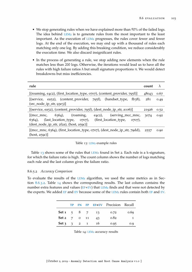
8.6 evaluation 103
• We stop generating rules when we have explained more than 90% of the failed logs.The idea behind LEM2 is to generate rules from the most important to the leastimportant. As the execution of LEM2 progresses, the rules cover fewer and fewerlogs. At the end of the execution, we may end up with a thousand of rules eachmatching only one log. By adding this breaking condition, we reduce considerablythe execution time. We also discard insignificant rules.
• In the process of generating a rule, we stop adding new elements when the rulematches less than 200 logs. Otherwise, the iterations would lead us to have all therules with high failure ratios λ but small signature proportions π. We would detectbreakdowns but miss inefficiencies.
rule count λ
[(roaming, e4c2), (first_location_type, 0707), (content_provider, 795f)] 48043 0.67
[(service, ea52), (content_provider, 795f), (handset_type, fb38),(src_node_ip_str, 93e3)]
281 0.49
[(service, ea52), (content_provider, 795f), (dest_node_ip_str, a106)] 21926 0.52
[(mcc_mnc, 6364), (roaming, e4c2), (serving_mcc_mnc,6364), (last_location_type, 0707), (first_location_type, 0707),(dest_node_ip_str, 2f2a), (host, a59c)]
3074 0.92
[(mcc_mnc, 6364), (first_location_type, 0707), (dest_node_ip_str, 79dd),(host, a59c)]
2557 0.90
Table 13: LEM2 example rules
Table 13 shows some of the rules that LEM2 found in Set 2. Each rule is a k-signature,for which the failure ratio is high. The count column shows the number of logs matchingeach rule and the last column gives the failure ratio.
8.6.5.2 Accuracy Comparison
To evaluate the results of the LEM2 algorithm, we used the same metrics as in Sec-tion 8.6.3.2. Table 14 shows the corresponding results. The last column contains thenumber extra features and values (EF+EV) that LEM2 finds and that were not detected bythe experts. We added EF and EV because some of the LEM2 rules contain both EF and EV.
TP FN FP EF+EV Precision Recall
Set 1 5 8 7 13 0.72 0.69
Set 2 7 0 11 43 0.82 1
Set 3 3 2 1 16 0.95 0.9
Table 14: LEM2 accuracy results
[ October 2, 2019 – Anomaly Detection and Root Cause Analysis v1.0 ]

104 proposed algorithm : arcd
The numbers of FP and FN are high due to two reasons: first, to deduct the rules, LEM2
conducts an analysis in the set of failed logs without comparing the set of failed logs andthe set of successful logs. For this reason, we have many false positives. Second, duringthe execution of LEM2, every time a rule is generated, its matching logs are excludedfrom the analysis. This may be the reason behind false negatives as the sets of logsrelated to two independent issues may overlap.
100 101 102 103 104 1050
0.2
0.4
0.6
0.8
1
count (logarithmic scale)
Fa
ilu
reR
ati
o
ARCD-MCARCD-INCOMPLEM2
Figure 47: Output from Set 3, signatures identified by ARCD-MC (major contributors), byARCD-INCOMP (incompatibilities), and LEM2. Each point corresponds to one
signature, with its failure ratio and the number of related logs.
Figure 47 shows the results obtained by ARCD and LEM2 on Set 3. Each point is ak-signature, the x value is the number of logs matching that signature and the y valueis its inefficiency. ARCD-MC refers to the signatures detected by the major contributordetection process. ARCD-INCOMP refers to the signatures detected in the process of in-compatibility detection. LEM2 refers to the signatures identified by LEM2. The horizontalline shows the inefficiency of the whole network. The figure shows that, in the specificuse case of root cause diagnosis in mobile networks, ARCD outperforms LEM2: Most ofthe signatures identified by ARCD have a higher failure ratio and a higher number oflogs compared to LEM2 signatures. We can also observe that the identified incompatibil-ity signatures are more inefficient but less frequent, in general, than the signatures ofmajor contributors.
8.6.5.3 Time Complexity
Let m be the number of features, k the maximum number of value per feature and n thenumber of logs. As the dependency analysis (equivalence classes, hierarchical depen-dencies and pruning) is only performed on a limited number of signatures (top fifty),its complexity is then O(1). Thus, the time complexity of major contributor detectionin our solution is equal to the complexity of top signature identification which is equal
[ October 2, 2019 – Anomaly Detection and Root Cause Analysis v1.0 ]

8.6 evaluation 105
to O(mkn). As m n, we can approximate the complexity to O(kn). So, in the worstcase, where a feature has a different value for each log, the complexity would be O(n2).Otherwise, in general, it is approximated to O(n). The same reasoning applies to incom-patibility detection. Its time complexity is equal to O(m2k2n). In the worst case, it isO(n3) and otherwise, O(n). As explained in [82], the complexity of the LEM2 algorithmis approximated to O(n3).
[ October 2, 2019 – Anomaly Detection and Root Cause Analysis v1.0 ]

[ October 2, 2019 – Anomaly Detection and Root Cause Analysis v1.0 ]
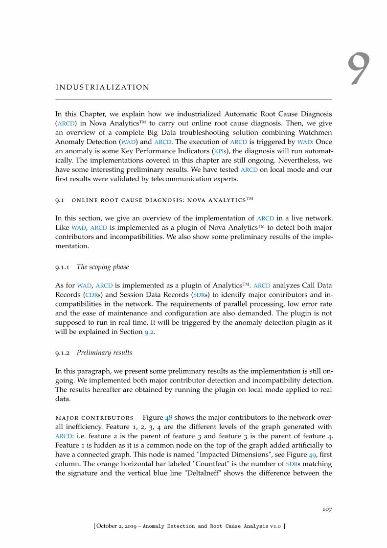
9I N D U S T R I A L I Z AT I O N
In this Chapter, we explain how we industrialized Automatic Root Cause Diagnosis(ARCD) in Nova Analytics™ to carry out online root cause diagnosis. Then, we givean overview of a complete Big Data troubleshooting solution combining WatchmenAnomaly Detection (WAD) and ARCD. The execution of ARCD is triggered by WAD: Oncean anomaly is some Key Performance Indicators (KPIs), the diagnosis will run automat-ically. The implementations covered in this chapter are still ongoing. Nevertheless, wehave some interesting preliminary results. We have tested ARCD on local mode and ourfirst results were validated by telecommunication experts.
9.1 online root cause diagnosis : nova analytics™
In this section, we give an overview of the implementation of ARCD in a live network.Like WAD, ARCD is implemented as a plugin of Nova Analytics™ to detect both majorcontributors and incompatibilities. We also show some preliminary results of the imple-mentation.
9.1.1 The scoping phase
As for WAD, ARCD is implemented as a plugin of Analytics™. ARCD analyzes Call DataRecords (CDRs) and Session Data Records (SDRs) to identify major contributors and in-compatibilities in the network. The requirements of parallel processing, low error rateand the ease of maintenance and configuration are also demanded. The plugin is notsupposed to run in real time. It will be triggered by the anomaly detection plugin as itwill be explained in Section 9.2.
9.1.2 Preliminary results
In this paragraph, we present some preliminary results as the implementation is still on-going. We implemented both major contributor detection and incompatibility detection.The results hereafter are obtained by running the plugin on local mode applied to realdata.
major contributors Figure 48 shows the major contributors to the network over-all inefficiency. Feature 1, 2, 3, 4 are the different levels of the graph generated withARCD: i.e. feature 2 is the parent of feature 3 and feature 3 is the parent of feature 4.Feature 1 is hidden as it is a common node on the top of the graph added artificially tohave a connected graph. This node is named "Impacted Dimensions", see Figure 49, firstcolumn. The orange horizontal bar labeled "Countfeat" is the number of SDRs matchingthe signature and the vertical blue line "DeltaIneff" shows the difference between the
107
[ October 2, 2019 – Anomaly Detection and Root Cause Analysis v1.0 ]
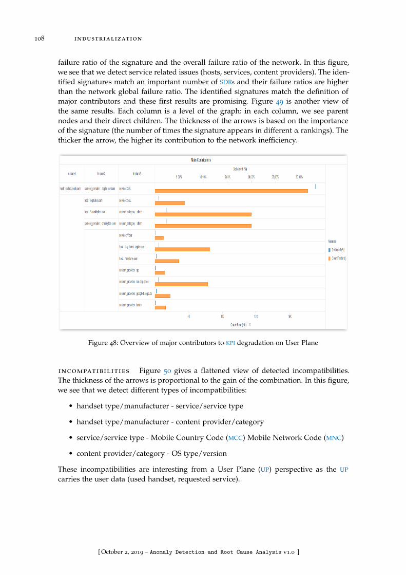
108 industrialization
failure ratio of the signature and the overall failure ratio of the network. In this figure,we see that we detect service related issues (hosts, services, content providers). The iden-tified signatures match an important number of SDRs and their failure ratios are higherthan the network global failure ratio. The identified signatures match the definition ofmajor contributors and these first results are promising. Figure 49 is another view ofthe same results. Each column is a level of the graph: in each column, we see parentnodes and their direct children. The thickness of the arrows is based on the importanceof the signature (the number of times the signature appears in different α rankings). Thethicker the arrow, the higher its contribution to the network inefficiency.
Figure 48: Overview of major contributors to KPI degradation on User Plane
incompatibilities Figure 50 gives a flattened view of detected incompatibilities.The thickness of the arrows is proportional to the gain of the combination. In this figure,we see that we detect different types of incompatibilities:
• handset type/manufacturer - service/service type
• handset type/manufacturer - content provider/category
• service/service type - Mobile Country Code (MCC) Mobile Network Code (MNC)
• content provider/category - OS type/version
These incompatibilities are interesting from a User Plane (UP) perspective as the UP
carries the user data (used handset, requested service).
[ October 2, 2019 – Anomaly Detection and Root Cause Analysis v1.0 ]
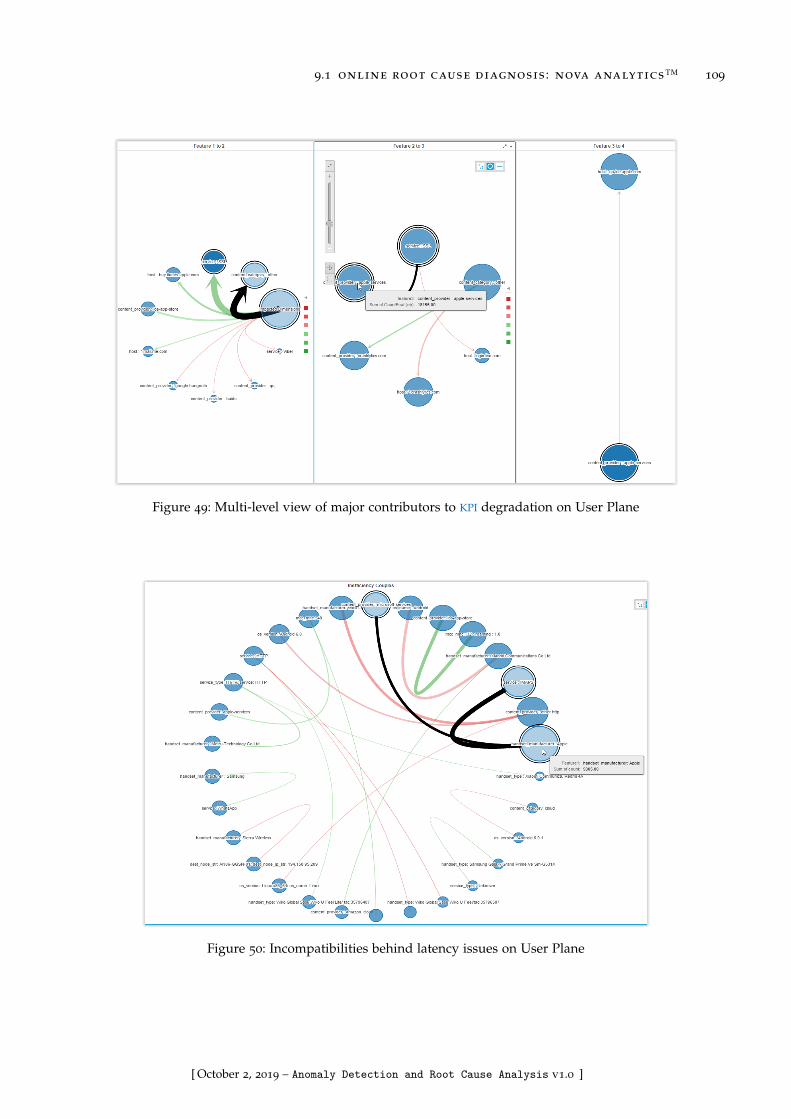
9.1 online root cause diagnosis : nova analytics™ 109
Figure 49: Multi-level view of major contributors to KPI degradation on User Plane
Figure 50: Incompatibilities behind latency issues on User Plane
[ October 2, 2019 – Anomaly Detection and Root Cause Analysis v1.0 ]
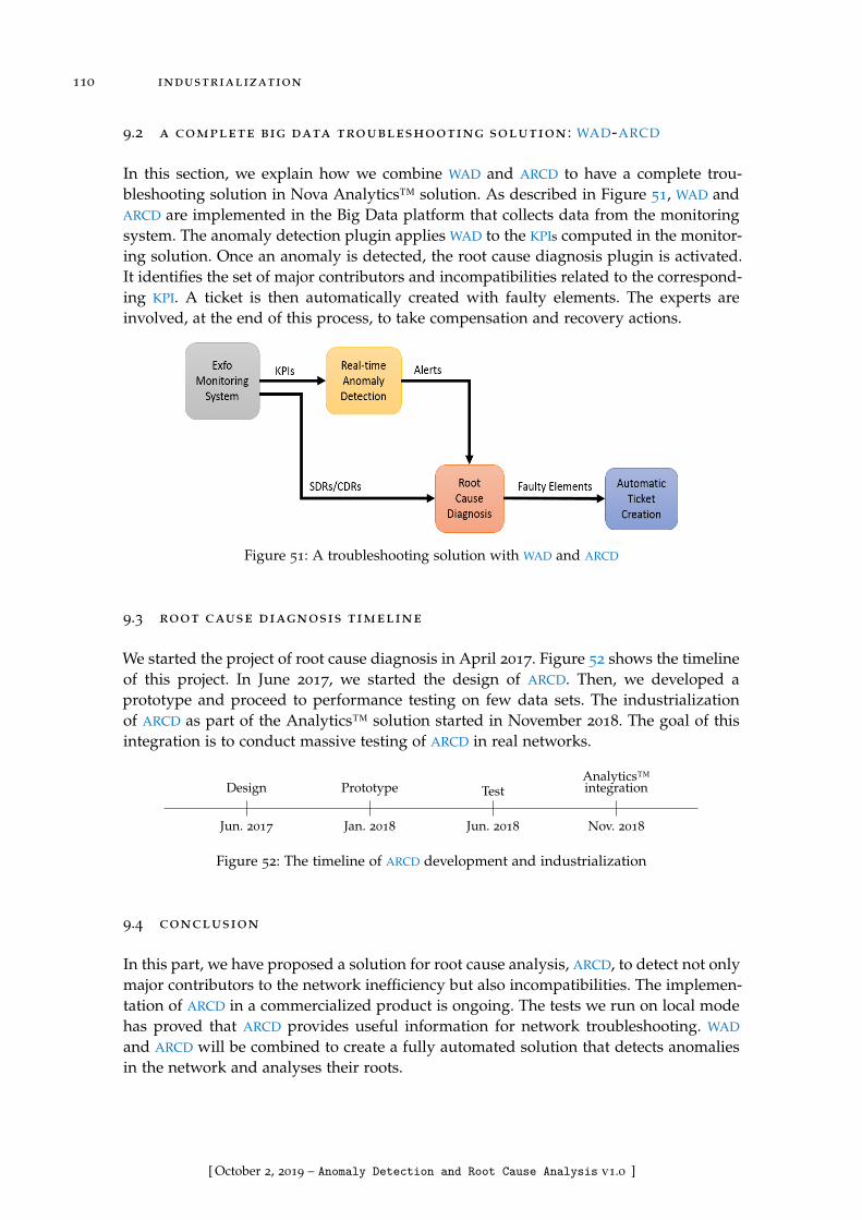
110 industrialization
9.2 a complete big data troubleshooting solution : WAD-ARCD
In this section, we explain how we combine WAD and ARCD to have a complete trou-bleshooting solution in Nova Analytics™ solution. As described in Figure 51, WAD andARCD are implemented in the Big Data platform that collects data from the monitoringsystem. The anomaly detection plugin applies WAD to the KPIs computed in the monitor-ing solution. Once an anomaly is detected, the root cause diagnosis plugin is activated.It identifies the set of major contributors and incompatibilities related to the correspond-ing KPI. A ticket is then automatically created with faulty elements. The experts areinvolved, at the end of this process, to take compensation and recovery actions.
Figure 51: A troubleshooting solution with WAD and ARCD
9.3 root cause diagnosis timeline
We started the project of root cause diagnosis in April 2017. Figure 52 shows the timelineof this project. In June 2017, we started the design of ARCD. Then, we developed aprototype and proceed to performance testing on few data sets. The industrializationof ARCD as part of the Analytics™ solution started in November 2018. The goal of thisintegration is to conduct massive testing of ARCD in real networks.
Jun. 2017
Design
Jan. 2018
Prototype
Jun. 2018
Test
Nov. 2018
Analytics™integration
Figure 52: The timeline of ARCD development and industrialization
9.4 conclusion
In this part, we have proposed a solution for root cause analysis, ARCD, to detect not onlymajor contributors to the network inefficiency but also incompatibilities. The implemen-tation of ARCD in a commercialized product is ongoing. The tests we run on local modehas proved that ARCD provides useful information for network troubleshooting. WAD
and ARCD will be combined to create a fully automated solution that detects anomaliesin the network and analyses their roots.
[ October 2, 2019 – Anomaly Detection and Root Cause Analysis v1.0 ]

Part IV
C O N C L U S I O N
[ October 2, 2019 – Anomaly Detection and Root Cause Analysis v1.0 ]

[ October 2, 2019 – Anomaly Detection and Root Cause Analysis v1.0 ]
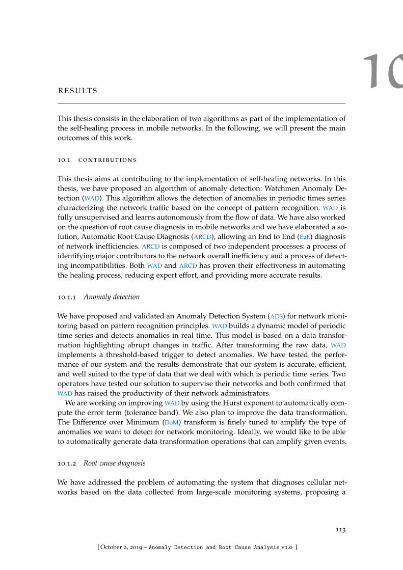
10R E S U LT S
This thesis consists in the elaboration of two algorithms as part of the implementation ofthe self-healing process in mobile networks. In the following, we will present the mainoutcomes of this work.
10.1 contributions
This thesis aims at contributing to the implementation of self-healing networks. In thisthesis, we have proposed an algorithm of anomaly detection: Watchmen Anomaly De-tection (WAD). This algorithm allows the detection of anomalies in periodic times seriescharacterizing the network traffic based on the concept of pattern recognition. WAD isfully unsupervised and learns autonomously from the flow of data. We have also workedon the question of root cause diagnosis in mobile networks and we have elaborated a so-lution, Automatic Root Cause Diagnosis (ARCD), allowing an End to End (E2E) diagnosisof network inefficiencies. ARCD is composed of two independent processes: a process ofidentifying major contributors to the network overall inefficiency and a process of detect-ing incompatibilities. Both WAD and ARCD has proven their effectiveness in automatingthe healing process, reducing expert effort, and providing more accurate results.
10.1.1 Anomaly detection
We have proposed and validated an Anomaly Detection System (ADS) for network moni-toring based on pattern recognition principles. WAD builds a dynamic model of periodictime series and detects anomalies in real time. This model is based on a data transfor-mation highlighting abrupt changes in traffic. After transforming the raw data, WAD
implements a threshold-based trigger to detect anomalies. We have tested the perfor-mance of our system and the results demonstrate that our system is accurate, efficient,and well suited to the type of data that we deal with which is periodic time series. Twooperators have tested our solution to supervise their networks and both confirmed thatWAD has raised the productivity of their network administrators.
We are working on improving WAD by using the Hurst exponent to automatically com-pute the error term (tolerance band). We also plan to improve the data transformation.The Difference over Minimum (DoM) transform is finely tuned to amplify the type ofanomalies we want to detect for network monitoring. Ideally, we would like to be ableto automatically generate data transformation operations that can amplify given events.
10.1.2 Root cause diagnosis
We have addressed the problem of automating the system that diagnoses cellular net-works based on the data collected from large-scale monitoring systems, proposing a
113
[ October 2, 2019 – Anomaly Detection and Root Cause Analysis v1.0 ]
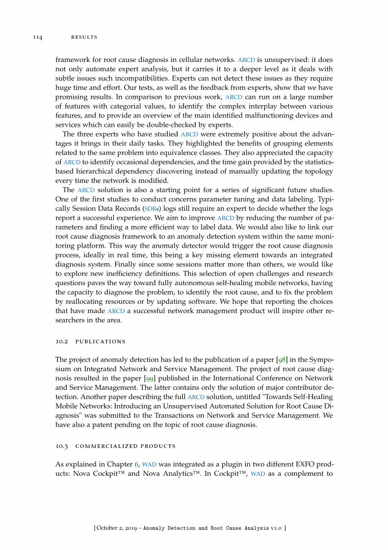
114 results
framework for root cause diagnosis in cellular networks. ARCD is unsupervised: it doesnot only automate expert analysis, but it carries it to a deeper level as it deals withsubtle issues such incompatibilities. Experts can not detect these issues as they requirehuge time and effort. Our tests, as well as the feedback from experts, show that we havepromising results. In comparison to previous work, ARCD can run on a large numberof features with categorial values, to identify the complex interplay between variousfeatures, and to provide an overview of the main identified malfunctioning devices andservices which can easily be double-checked by experts.
The three experts who have studied ARCD were extremely positive about the advan-tages it brings in their daily tasks. They highlighted the benefits of grouping elementsrelated to the same problem into equivalence classes. They also appreciated the capacityof ARCD to identify occasional dependencies, and the time gain provided by the statistics-based hierarchical dependency discovering instead of manually updating the topologyevery time the network is modified.
The ARCD solution is also a starting point for a series of significant future studies.One of the first studies to conduct concerns parameter tuning and data labeling. Typi-cally Session Data Records (SDRs) logs still require an expert to decide whether the logsreport a successful experience. We aim to improve ARCD by reducing the number of pa-rameters and finding a more efficient way to label data. We would also like to link ourroot cause diagnosis framework to an anomaly detection system within the same moni-toring platform. This way the anomaly detector would trigger the root cause diagnosisprocess, ideally in real time, this being a key missing element towards an integrateddiagnosis system. Finally since some sessions matter more than others, we would liketo explore new inefficiency definitions. This selection of open challenges and researchquestions paves the way toward fully autonomous self-healing mobile networks, havingthe capacity to diagnose the problem, to identify the root cause, and to fix the problemby reallocating resources or by updating software. We hope that reporting the choicesthat have made ARCD a successful network management product will inspire other re-searchers in the area.
10.2 publications
The project of anomaly detection has led to the publication of a paper [98] in the Sympo-sium on Integrated Network and Service Management. The project of root cause diag-nosis resulted in the paper [99] published in the International Conference on Networkand Service Management. The latter contains only the solution of major contributor de-tection. Another paper describing the full ARCD solution, untitled "Towards Self-HealingMobile Networks: Introducing an Unsupervised Automated Solution for Root Cause Di-agnosis" was submitted to the Transactions on Network and Service Management. Wehave also a patent pending on the topic of root cause diagnosis.
10.3 commercialized products
As explained in Chapter 6, WAD was integrated as a plugin in two different EXFO prod-ucts: Nova Cockpit™ and Nova Analytics™. In Cockpit™, WAD as a complement to
[ October 2, 2019 – Anomaly Detection and Root Cause Analysis v1.0 ]

10.3 commercialized products 115
the monitoring system. In concrete terms, it detects anomalies in the input/output ofnetwork probes and other monitoring tools. In Analytics™, WAD is used to manage ser-vice quality by detecting anomalies in service quality indicators. In Chapter 9, we haveshown briefly how ARCD was integrated in Analytics™ to diagnose issues at differentpoints of the network. This implementation is still ongoing.
[ October 2, 2019 – Anomaly Detection and Root Cause Analysis v1.0 ]

[ October 2, 2019 – Anomaly Detection and Root Cause Analysis v1.0 ]
11F U T U R E W O R K
In this thesis, we have presented two algorithms relevant to the question of self-healingnetworks. The first algorithm, Watchmen Anomaly Detection (WAD), allows to detectanomalies in periodic time series. The second algorithm, Automatic Root Cause Diag-nosis (ARCD), allows to diagnose the network and identify the root causes of issues.Despite the efficiency of our solutions, they still have shortcomings. In the following, wewill propose some potential improvements to our algorithms. Then, we will finish withresearch questions that we started studying in this thesis.
11.1 potential improvements
Regarding anomaly detection, our solution WAD has promising results. However, manyimprovements are possible. First, WAD has a few parameters to be tuned manually. Au-tomating the parameter setting would make the solution applicable to different use caseswithout any human intervention. Second, the Difference over Minimum (DoM) transformwe have adopted in WAD allows the detection of abrupt changes in time series. Ideally, acomplete anomaly detection solution should be able to detect different types of anoma-lies. Third, our solution works on periodic data and is applicable to constant time series.However, it does not fit chaotic time series. A general solution of anomaly detection intime series would cover both periodic and chaotic time series. An extra work may be toadapt WAD to detect patterns in chaotic time series.
Our solution of root cause diagnosis, ARCD, has proven its efficiency in identifyinginefficiency major contributors and incompatibilities. Nevertheless, it is still limited inmany aspects. First, ARCD has few parameters that needed to be set by experts and em-pirical tests. Second, in the case of features having a large number of possible valuessuch as International Mobile Subscriber Identitys (IMSIs), the execution time is polyno-mial. Some optimizations may be carried out to address this specific case. Third, ARCD
detect incompatibilities involving two elements. While the incompatibility detection pro-cess can be applicable to identify incompatibilities involving three or more elements, thetime complexity may grow exponentially. Last but not least, to identify the root of issues,ARCD explores equivalence classes (mutually dependent elements) and hierarchical de-pendencies. Other types of dependencies could be added to the process to have a morerobust and precise diagnosis.
11.2 next steps
As a future work, we will focus on automating the compensation and the recoveryprocesses to have a fully self-healing network. The compensation task consists in de-termining a quick and temporary operations to circumvent network issues and restoreservice access as fast as possible. For example, one may modify the route of the traffic
117
[ October 2, 2019 – Anomaly Detection and Root Cause Analysis v1.0 ]
118 future work
to bypass a non-functional device. The recovery process consists in finding a permanentsolution to network issues such as replacing broken equipment. We plan also to workin a more pro-active manner, which means that we would like to predict anomalies anddifferent network issues before they happen. This would be possible if we study thesequence of events preceding network issues. We would also like to extend the scopeof our analysis to cloud infrastructures and computer networks in general. We aim totest and validate our solutions on these types of networks. Regarding the data analysisaspect of our work, we plan to extend our work to manipulating unstructured data suchas system event logs. Another interesting point is the use of Data Assimilation whichcombines data analysis with theoretical modeling. It creates dynamic models that donot diverge from the real state of the system by combining a mathematical model withreal time observations.
11.3 open research questions
This thesis contributes to the understanding of some research questions, which are notfully addressed by the scientific community. The main question behind this work isthe concept of Self-healing networks. Despite the many specifications that describe thefunctioning of self healing network, current mobile networks still rely importantly onhuman experts in the troubleshooting tasks. Another question relevant to this work is theuniversality of anomaly detection. While the literature contains hundreds if not thousandsof anomaly detection solutions, each domain still has its specificity. Therefore, thereis no universal solution applicable independently of the context. The question of Endto End (E2E) network diagnosis is also tightly related to this work. This question is stillopen as devices and applications produce heterogeneous data structures that cannot beassimilated and processed by monitoring systems without the help of experts.
[ October 2, 2019 – Anomaly Detection and Root Cause Analysis v1.0 ]

Part V
A P P E N D I X
[ October 2, 2019 – Anomaly Detection and Root Cause Analysis v1.0 ]

[ October 2, 2019 – Anomaly Detection and Root Cause Analysis v1.0 ]
AD E V E L O P M E N T E N V I R O N M E N T
We describe, in the following, the development environment and the testing environ-ment used in the implementation of Watchmen Anomaly Detection (WAD) and AutomaticRoot Cause Diagnosis (ARCD).
a.1 general description
We created a development environment for the prototyping phase of anomaly detectionand root cause diagnosis. The choice of the tools is based on practical considerations.We started with the Linux based Operating System (OS) Ubuntu version 16.04, upgradedthen to 18.04. To process data, we used the programming language Python 2.7 and 3.5.We used the Integrated Development Environment (IDE) PyCharm version 2016.3.3. Fordata exploration, we used the Interactive Python (IPython) based application Jupyter 4.4.0.The data used in the prototyping are sample stored in Comma Separated Values (CSV)files and a MySQL database version 14.14 distribution 5.7.26.
a.2 python libraries
The high level programming language Python offers a large number of data analysislibraries. These libraries are open source mostly under an Massachusetts Institute ofTechnology (MIT) or a Berkeley Software Distribution (BSD) licenses. To install these li-braries, we used the package manager PIP Installs Packages (PIP). We created an isolatedPython environment via the tool Virtualenv containing all the needed packages and theirdependencies. Having a virtual environment allows multiple versions of the same pack-age to coexist in the same system without interfering. A Python virtual environmentis also easily replicated. Table 15 contains an overview of the libraries we used in ourimplementation along with the corresponding versions.
a.3 big data environment
To validate our algorithms, we used a Big Data cluster designed for large scale dataprocessing. The parallel processing by the different nodes of the cluster is coordinated bySpark running on the top of Hadoop. The spark jobs are scheduled by the task managerOAR. Spark distributes the multidimensional calculations on several nodes allowing asignificant decrease of the execution time. The spark jobs we ran on this platform arepython scripts. We ran them either as interactive jobs or passive jobs. In both cases, weuse a logging function to track the evolution of the process.
121
[ October 2, 2019 – Anomaly Detection and Root Cause Analysis v1.0 ]
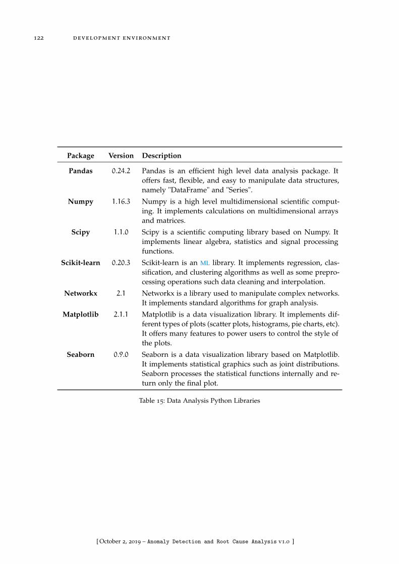
122 development environment
Package Version Description
Pandas 0.24.2 Pandas is an efficient high level data analysis package. Itoffers fast, flexible, and easy to manipulate data structures,namely "DataFrame" and "Series".
Numpy 1.16.3 Numpy is a high level multidimensional scientific comput-ing. It implements calculations on multidimensional arraysand matrices.
Scipy 1.1.0 Scipy is a scientific computing library based on Numpy. Itimplements linear algebra, statistics and signal processingfunctions.
Scikit-learn 0.20.3 Scikit-learn is an ML library. It implements regression, clas-sification, and clustering algorithms as well as some prepro-cessing operations such data cleaning and interpolation.
Networkx 2.1 Networkx is a library used to manipulate complex networks.It implements standard algorithms for graph analysis.
Matplotlib 2.1.1 Matplotlib is a data visualization library. It implements dif-ferent types of plots (scatter plots, histograms, pie charts, etc).It offers many features to power users to control the style ofthe plots.
Seaborn 0.9.0 Seaborn is a data visualization library based on Matplotlib.It implements statistical graphics such as joint distributions.Seaborn processes the statistical functions internally and re-turn only the final plot.
Table 15: Data Analysis Python Libraries
[ October 2, 2019 – Anomaly Detection and Root Cause Analysis v1.0 ]

BS y m b o l i c A g g r e g a t e A p p r o x i m a t i o n
Symbolic Aggregate Approximation (SAX) is an algorithm that transforms a numericaltime series to a sequence of strings. This transformation aims at reducing the size ofthe data set and removing noise. SAX offers an efficient data representation that can fitclassification and forecasting purposes. SAX is applicable on timestamped data in thecontext of sequential analysis. SAX has two main steps:
• Piecewise Aggregate Approximation (PAA)
• Transforming PAA output into sequences of symbols/letters.
b.1 Piecewise Aggregate Approximation
PAA takes as an input a time series of length n. Then, it splits the time series into wsequences of the same size. We compute afterwards, the mean of each sequence andcreate a new times series of length w containing the calculated averages. This step hastwo main advantages. First, it reduce the size of the time series from n to w whichalleviates the processing load. Second, it is robust to noise and outliers: The obtainedtime series is smoother than the original one. It has less significant peaks and dips.The moderation of extreme values at the early stages of the processing makes the datamodeling more accurate.
b.2 transformation into symbols
This step consists in converting numerical data into a sequence of symbols. The symbolsare equiprobable and their number k is predefined. k controls the sensitivity of thealgorithm. We start with the assumption that the values of the time series after the PAA
transformation have a continuous Gaussian distribution. We split the Gaussian curveinto k equiprobable intervals. Each interval is represented by a symbol: a,b, c.... Then,we map each time series value to the symbol representing its corresponding interval.This process transforms the time series into a sequence of symbols. This sequence couldinclude some repetitive patterns that are more visible with this discretization.
b.3 SAX applications
SAX is useful as a first processing step preceding another clustering/forecasting algo-rithm. As SAX reduces the size of data and limits the number of possible symbols, itallows the application of complex algorithms that take a large number of iterations be-fore convergence. Another important aspect of SAX is its ability to highlight patterns inthe data. These patterns can be clustered for classical classification aims or for anomalydetection. The patterns can also be used to build a tree that models the variations of the
123
[ October 2, 2019 – Anomaly Detection and Root Cause Analysis v1.0 ]

124 sax algorithm
time series. By navigating the tree structure, one may predict the next symbol which isequivalent to the interval of the next value.
[ October 2, 2019 – Anomaly Detection and Root Cause Analysis v1.0 ]

CP r i n c i p a l C o m p o n e n t A n a l y s i s
Principal Component Analysis (PCA) is a feature extraction technique. It allows to reducethe dimensionality of data with a minimal information loss. PCA transforms the originalfeatures into fewer features by the means of linear combinations. The coefficients of thelinear combinations are optimally adjusted to retain as much as possible of the originalvariance of data. Reducing dimensions eases data processing and makes the modelsmore controllable. In addition, the visualization of high dimensional data is a complextask. Reducing the number of features allows to visualize data easily and to exploredata patterns. PCA is applicable to numerical data. Depending on the context, PCA canbe either a preprocessing step or the core of the processing task.
c.1 steps
The first step of PCA is to standardize data. As features have different significance andthus different units and ranges, rescaling the data is essential. Otherwise, features withrelatively small values will have a negligible impact on the model. Thus, we normalizethe data so each feature has a zero mean and a unit variance. The next step is to createfew new features containing the maximum of the variance. To do so, we calculate thecovariance matrix of the original data. Then, we compute its eigenvectors and eigen-values. The eigenvectors are uncorrelated and thus there is no information redundancy.The eigenvalues represent the variance carried by each eigenvector. We rank the eigen-vectors by their corresponding eigenvalues and take only the k first ones to be the newfeatures. The data samples are then projected on the basis formed by the new features.This way, we reduce the dimensionality of data with a minimum information loss.
c.2 applications
The PCA can be used in different contexts. As a tool of dimensionality reduction, the PCA
allows to reduce the number of features and eliminate information redundancy. Conse-quently, it is used as a key step in the preprocessing before going to the core of the dataprocessing with complex algorithms such as Support Vector Machine (SVM) and neuralnetworks. Furthermore, PCA can be used as a standalone algorithm serving differentpurposes. For example, PCA can be used in the case of noise filtering. The eigenvectorswith low eigenvalues are the components with low variance. These components containmainly the noise of the data. As PCA keeps only the eigenvectors with high eigenval-ues to be the new features, the noise is removed. Another interesting application is thedetection of anomalies. The anomalies are situated in the components with lows vari-ance because of their rarity. Therefore, by studying these components, one may detectanomalies.
125
[ October 2, 2019 – Anomaly Detection and Root Cause Analysis v1.0 ]

[ October 2, 2019 – Anomaly Detection and Root Cause Analysis v1.0 ]
DL e a r n i n g f r o m E x a m p l e s M o d u l e , ve r s i o n 2
Learning from Examples Module, version 2 (LEM2) is an algorithm of rule inductionbased on rough set theory. It allows to explain a categorial dependent/decision variablewith a set of categorial independent variables. LEM2 transforms the samples of a multi-dimensional data set to a list of feature-value pairs. Then, it highlights the associationsof subsets of feature-value pairs with each value of the decision variable. The aim ofLEM2 is to create association rules that allow to infer the value of the dependent vari-able based on the the values of independent variables in a deterministic and accurateway. The extracted rules can be descriptive or predictive. They can be used either toexplain a non-trivial classification of data samples or to predict the following values ofthe decision variable.
d.1 steps
LEM2 operates in an incremental way until covering the complete data set. The data set issubdivided into subsets with regards to the decision variable. Then in each subset, LEM2
identifies the most frequent signature (a collection of feature-value pairs) that does notappear in any other subset. If the extracted signature covers all the samples of the subset,then this signature is sufficient to identify the subset. The resulting decision rule wouldbe signature → decision variable value. In the other case, LEM2 identifies the second mostfrequent signature. This process is iterated until covering all the samples of the subset.It is also replicated in all the subsets. This way, we have a set of association rules foreach value of the decision variable. At the end of this process, the rules are optimizedby removing uninformative feature-value pairs from the signatures. Superfluous rulesare also removed from the rule set.
d.2 applications
LEM2 is applicable to labeled categorial data. It can serve two different purposes: datadescription and prediction. In the first case, the data may have a label that is not straight-forward to understand. LEM2 creates association rules that explain how the label can beinferred from more meaningful variables. LEM2 can also point causalities between vari-ables. In the second case, LEM2 is used to predict the label. The algorithm learns the rulesduring the training phase. Then, it decides the label of the coming samples on the basisof the deduced rules. LEM2 operates in a greedy way. Thus it may converge to a local ora global optimum. In some contexts, a local optimum is acceptable. Depending on thesize and the dimensionality of the data set, the execution time may grow significantlywith the nested loops. It is possible to add breaking conditions to the loops of LEM2 toreduce the execution time at the expense of the accuracy.
127
[ October 2, 2019 – Anomaly Detection and Root Cause Analysis v1.0 ]

[ October 2, 2019 – Anomaly Detection and Root Cause Analysis v1.0 ]

B I B L I O G R A P H Y
[1] “3GPP; Technical Specification Group Services and System Aspects; Telecommu-nication management; Charging management; Charging Data Record (CDR) pa-rameter description, TS 32.298, v15.5.1,” Tech. Rep., 2018.
[2] “5G vision, white paper,” Samsung Electronics Co., Tech. Rep., 2015.
[3] “5G; Service requirements for next generation new services and markets, TS22.261, V15.5.0,” 3GPP, Tech. Rep., 2018.
[4] “5G: A technology vision, white paper,” Huawei Technologies Co., Tech. Rep.,2013.
[5] P. S. Addison, The illustrated wavelet transform handbook: introductory theory andapplications in science, engineering, medicine and finance. 2017.
[6] B. Agarwal and N. Mittal, “Hybrid approach for detection of anomaly networktraffic using data mining techniques,” Procedia Technology, 2012.
[7] A. Agresti, An introduction to categorical data analysis. 2018.
[8] M. Ahmed, A. N. Mahmood, and J. Hu, “A survey of network anomaly detectiontechniques,” Journal of Network and Computer Applications, 2016.
[9] G. A. Akpakwu, B. J. Silva, G. P. Hancke, and A. M. Abu-Mahfouz, “A surveyon 5G networks for the internet of things: Communication technologies and chal-lenges,” IEEE Access, 2018.
[10] S. Axelsson, “Intrusion detection systems: A survey and taxonomy,” Tech. Rep.,2000.
[11] P. Barford, J. Kline, D. Plonka, and A. Ron, “A signal analysis of network trafficanomalies,” in Proc. of ACM SIGCOMM Workshop IMW, 2002.
[12] P. Berezinski, B. Jasiul, and M. Szpyrka, “An entropy-based network anomalydetection method,” Entropy, 2015.
[13] G. Bergland, “A guided tour of the fast fourier transform,” IEEE spectrum, 1969.
[14] M. Bianchini and F. Scarselli, “On the complexity of neural network classifiers: Acomparison between shallow and deep architectures,” IEEE Transactions on NeuralNetworks and Learning Systems, 2014.
[15] H. Bozdogan, “Model selection and Akaike’s information criterion (AIC): Thegeneral theory and its analytical extensions,” Psychometrika, 1987.
[16] A. P. Bradley, “The use of the area under the ROC curve in the evaluation ofmachine learning algorithms,” Pattern recognition, 1997.
[17] S. Brady, D. Magoni, J. Murphy, H. Assem, and A. O. Portillo-Dominguez, “Anal-ysis of machine learning techniques for anomaly detection in the internet ofthings,” in Latin American Conference on Computational Intelligence (LA-CCI), 2018.
129
[ October 2, 2019 – Anomaly Detection and Root Cause Analysis v1.0 ]

130 bibliography
[18] D. Brauckhoff, X. Dimitropoulos, A. Wagner, and K. Salamatian, “Anomaly ex-traction in backbone networks using association rules,” in Proceedings of the ACMSIGCOMM conference on Internet measurement, 2009.
[19] P. J. Brockwell, R. A. Davis, and M. V. Calder, Introduction to time series and fore-casting. 2002.
[20] M. Cairo, G. Farina, and R. Rizzi, “Decoding hidden markov models faster thanviterbi via online matrix-vector (max, +)-multiplication,” in AAAI Conference onArtificial Intelligence, 2016.
[21] R. N. Calheiros, E. Masoumi, R. Ranjan, and R. Buyya, “Workload prediction us-ing ARIMA model and its impact on cloud applications’ QoS,” IEEE Transactionson Cloud Computing, 2015.
[22] G. Casella and R. L. Berger, Statistical inference. 2002.
[23] M. Çelik, F. Dadaser-Çelik, and A. S. Dokuz, “Anomaly detection in tempera-ture data using dbscan algorithm,” in International Symposium on Innovations inIntelligent Systems and Applications (INISTA), 2011.
[24] V. Chandola, A. Banerjee, and V. Kumar, “Outlier detection: A survey,” ACMComputing Surveys, 2007.
[25] V. Chandola, A. Banerjee, and V. Kumar, “Anomaly detection: A survey,” ACMcomputing surveys (CSUR), 2009.
[26] C. Chang and C. Lin, “LIBSVM: a library for support vector machines,” ACMTIST, 2011.
[27] W. G. Cochran, Sampling techniques. 2007.
[28] A. d’Aspremont, F. R. Bach, and L. E. Ghaoui, “Full regularization path for sparseprincipal component analysis,” in International Conference on Machine Learning,2007.
[29] J. Davis and M. Goadrich, “The relationship between Precision-Recall and ROCcurves,” in International conference on Machine learning, 2006.
[30] Day, William H. E. and Edelsbrunner, Herbert, “Efficient algorithms for agglom-erative hierarchical clustering methods,” Journal of Classification, 1984.
[31] “Digital cellular telecommunications system (Phase 2+); Universal Mobile Telecom-munications System (UMTS); LTE; Network architecture, TS 23.002, V12.5.0,”3GPP, Tech. Rep., 2015.
[32] G. Dimopoulos, I. Leontiadis, P. Barlet-Ros, K. Papagiannaki, and P. Steenkiste,“Identifying the root cause of video streaming issues on mobile devices,” inCoNEXT, 2015.
[33] J. J. Dongarra and F. Sullivan, “Guest editors introduction to the top 10 algo-rithms,” Computing in Science and Engineering, 2000.
[34] Z. Du, L. Ma, H. Li, Q. Li, G. Sun, and Z. Liu, “Network traffic anomaly detec-tion based on wavelet analysis,” in International Conference on Software EngineeringResearch, Management and Applications, SERA, 2018.
[ October 2, 2019 – Anomaly Detection and Root Cause Analysis v1.0 ]

bibliography 131
[35] O. Eluwole, N. Udoh, M. Ojo, C. Okoro, and A. Akinyoade, “From 1G to 5G,what next?” IAENG International Journal of Computer Science, 2018.
[36] J. M. Estevez-Tapiador, P. Garcia-Teodoro, and J. E. Diaz-Verdejo, “Anomaly de-tection methods in wired networks: A survey and taxonomy,” Computer Commu-nications, 2004.
[37] “Evolved Universal Terrestrial Radio Access (E-UTRA) and Evolved UniversalTerrestrial Radio Access Network (E-UTRAN); Overall description, TS 36.300,V9.4.0,” 3GPP, Tech. Rep., 2010.
[38] S. Feng and E. Seidel, “Self-organizing networks (son) in 3gpp long term evolu-tion,” Nomor Research GmbH, Munich, Germany, 2008.
[39] R. Fontugne and K. Fukuda, “A Hough-transform-based anomaly detector withan adaptive time interval,” in Proc. of ACM SAC, 2011.
[40] S. Fortes, A. Aguilar Garcia, J. A. Fernandez-Luque, A. Garrido, and R. Barco,“Context-aware self-healing: User equipment as the main source of informationfor small-cell indoor networks,” IEEE Vehicular Technology Magazine, 2016.
[41] R. Froehlich, Knowledge base radio and core network prescriptive root cause analysis,US Patent Application 14/621,101, 2016.
[42] M. M. M. Fuad and P. Marteau, “Towards a faster symbolic aggregate approxi-mation method,” CoRR, 2013.
[43] S. R. Gaddam, V. V. Phoha, and K. S. Balagani, “K-means+id3: A novel method forsupervised anomaly detection by cascading k-means clustering and ID3 decisiontree learning methods,” IEEE Trans. Knowl. Data Eng., 2007.
[44] P. Garcia-Teodoro, J. Diaz-Verdejo, G. Maciá-Fernández, and E. Vázquez, “Anomaly-based network intrusion detection: Techniques, systems and challenges,” comput-ers & security, 2009.
[45] A. Garg, “Digital society from 1G to 5G: A comparative study,” InternationalJournal of Application or Innovation in Engineering & Management, 2014.
[46] G. Giacinto, F. Roli, and L. Didaci, “Fusion of multiple classifiers for intrusiondetection in computer networks,” Pattern recognition letters, 2003.
[47] P. Gogoi, R. Das, B. Borah, and D. K. Bhattacharyya, “Efficient rule set generationusing rough set theory for classification of high dimensional data,” IJSSAN, 2011.
[48] A. Gómez-Andrades, P. M. Luengo, I. Serrano, and R. Barco, “Automatic rootcause analysis for LTE networks based on unsupervised techniques,” IEEE Trans.Vehicular Technology, 2016.
[49] “GSM/EDGE radio access network (GERAN); overall description, TS 43.051, v8.0.0,”3GPP, Tech. Rep., 2009.
[50] F. Guigou, P. Collet, and P. Parrend, “Anomaly detection and motif discovery insymbolic representations of time series,” CoRR, 2017.
[51] F. Guigou, P. Collet, and P. Parrend, “The artificial immune ecosystem: A bio-inspired meta-algorithm for boosting time series anomaly detection with expertinput,” in Applications of Evolutionary Computation, 2017.
[ October 2, 2019 – Anomaly Detection and Root Cause Analysis v1.0 ]

132 bibliography
[52] H. Guo and C. S. Burrus, “Wavelet transform based fast approximate Fouriertransform,” in IEEE International Conference on Acoustics, Speech, and Signal Pro-cessing, 1997.
[53] M. Gupta, J. Gao, C. C. Aggarwal, and J. Han, “Outlier detection for temporaldata: A survey,” IEEE Transactions on Knowledge and Data Engineering, 2014.
[54] B. Hamzeh, Network failure detection and prediction using signal measurements, PatentUS9100339B1, 2014.
[55] T. Han, Y. Lan, L. Xiao, B. Huang, and K. Zhang, “Event detection with vectorsimilarity based on fourier transformation,” in Proc. of IEEE ICCSSE, 2014.
[56] A. Hanemann, “A hybrid rule-based/case-based reasoning approach for servicefault diagnosis,” in International Conference on Advanced Information Networkingand Applications AINA, 2006.
[57] F. van Harmelen, V. Lifschitz, and B. W. Porter, Eds., Handbook of Knowledge Rep-resentation. 2008.
[58] F. Harrou, F. Kadri, S. Chaabane, C. Tahon, and Y. Sun, “Improved principalcomponent analysis for anomaly detection: Application to an emergency depart-ment,” Computers & Industrial Engineering, 2015.
[59] N. A. Heard, D. J. Weston, K. Platanioti, D. J. Hand, et al., “Bayesian anomalydetection methods for social networks,” The Annals of Applied Statistics, 2010.
[60] J. J. Hildebrand, System and method for allocating resources based on events in a net-work environment, Patent US8788654B2, 2010.
[61] B. Horst and K. Abraham, Data mining in time series databases. 2004.
[62] W. Hu, Y. Liao, and V. R. Vemuri, “Robust support vector machines for anomalydetection in computer security,” in Proc. of IEEE ICMLA, 2003.
[63] Y. Huang, Service problem diagnosis for mobile wireless networks, Patent WO2012113436A1,2016.
[64] M. A. Imran and A. Zoha, “Challenges in 5g: How to empower SON with bigdata for enabling 5g,” IEEE Network, 2014.
[65] Z. Jadidi, V. Muthukkumarasamy, E. Sithirasenan, and M. Sheikhan, “Flow-basedanomaly detection using neural network optimized with GSA algorithm,” in Proc.of IEEE ICDCS, 2013.
[66] A. Y. Javaid, Q. Niyaz, W. Sun, and M. Alam, “A deep learning approach fornetwork intrusion detection system,” ICST Trans. Security Safety, 2016.
[67] Y. Jin, N. G. Duffield, A. Gerber, P. Haffner, S. Sen, and Z. Zhang, “Nevermind,the problem is already fixed: Proactively detecting and troubleshooting customerDSL problems,” in CoNEXT, 2010.
[68] C. Kane, System and method for identifying problems on a network, Patent US20150019916A1,2015.
[69] W. Kellerer, A. Basta, P. Babarczi, A. Blenk, M. He, M. Klügel, and A. M. Alba,“How to measure network flexibility? a proposal for evaluating softwarized net-works,” IEEE Communications Magazine, 2018.
[ October 2, 2019 – Anomaly Detection and Root Cause Analysis v1.0 ]

bibliography 133
[70] E. J. Keogh, J. Lin, and A. W. Fu, “HOT SAX: efficiently finding the most unusualtime series subsequence,” in Proc. of IEEE ICDM, 2005.
[71] E. Keogh, S. Chu, D. Hart, and M. Pazzani, “Segmenting time series: A surveyand novel approach,” in Data mining in time series databases, 2004.
[72] S. Khalid, T. Khalil, and S. Nasreen, “A survey of feature selection and featureextraction techniques in machine learning,” in Science and Information Conference(SAI), 2014, 2014.
[73] L. Khan, M. Awad, and B. Thuraisingham, “A new intrusion detection systemusing support vector machines and hierarchical clustering,” The VLDB journal,2007.
[74] E. J. Khatib, R. Barco, A. Gómez-Andrades, P. M. Luengo, and I. Serrano, “Datamining for fuzzy diagnosis systems in LTE networks,” Expert Syst. Appl., 2015.
[75] E. J. Khatib, R. Barco, P. M. Luengo, I. de la Bandera, and I. Serrano, “Self-healingin mobile networks with Big Data,” IEEE Communications Magazine, 2016.
[76] E. J. Khatib, “Data analytics and knowledge discovery for root cause analysis inlte self-organizing networks,” PhD dissertation, University of Malaga, 2017.
[77] D. B. Kiesekamp, T. Pilon, and R. Bolder, System and method of visualizing mostunhealthy network elements within a network or data center, Patent US20160183109A1,2016.
[78] G. Kim, S. Lee, and S. Kim, “A novel hybrid intrusion detection method integrat-ing anomaly detection with misuse detection,” Expert Systems with Applications,2014.
[79] P. V. Klaine, M. A. Imran, O. Onireti, and R. D. Souza, “A survey of machinelearning techniques applied to self-organizing cellular networks,” IEEE Commu-nications Surveys and Tutorials, 2017.
[80] R. Kohavi, “A study of cross-validation and bootstrap for accuracy estimationand model selection,” in International Joint Conference on Artificial Intelligence, IJ-CAI, 1995.
[81] A. Lakhina, M. Crovella, and C. Diot, “Diagnosing network-wide traffic anoma-lies,” in Proc. of ACM SIGCOMM, 2004.
[82] O. Leifler, “Comparison of lem2 and a dynamic reduct classification algorithm,”Master’s thesis, 2002.
[83] F. Li and M. Thottan, “End-to-end service quality measurement using source-routed probes,” in IEEE International Conference on Computer Communications (IN-FOCOM), 2006.
[84] J. Li, W. Pedrycz, and I. Jamal, “Multivariate time series anomaly detection: Aframework of hidden markov models,” Appl. Soft Comput., 2017.
[85] J. Liu, F. Liu, and N. Ansari, “Monitoring and analyzing big traffic data of alarge-scale cellular network with Hadoop,” IEEE Network, 2014.
[86] X. Liu, G. Chuai, W. Gao, and K. Zhang, “GA-AdaBoostSVM classifier empow-ered wireless network diagnosis,” EURASIP Journal on Wireless Comm. and Net-working, 2018.
[ October 2, 2019 – Anomaly Detection and Root Cause Analysis v1.0 ]

134 bibliography
[87] “Looking ahead to 5G, white paper,” Nokia networks, Tech. Rep., 2014.
[88] “LTE; Evolved Universal Terrestrial Radio Access Network (E-UTRAN); Self-configuring and self-optimizing network (SON) use cases and solutions, TS 36.902,V9.2.0,” 3GPP, Tech. Rep., 2010.
[89] W. Lu and A. A. Ghorbani, “Network anomaly detection based on wavelet anal-ysis,” EURASIP J. Adv. Sig. Proc., 2009.
[90] P. M. Luengo, R. Barco, E. Cruz, A. Gómez-Andrades, E. J. Khatib, and N. Faour,“A method for identifying faulty cells using a classification tree-based UE diag-nosis in LTE,” EURASIP J. Wireless Comm. and Networking, 2017.
[91] J. Luo and S. M. Bridges, “Mining fuzzy association rules and fuzzy frequencyepisodes for intrusion detection,” International Journal of Intelligent Systems, 2000.
[92] J. Ma and S. Perkins, “Time-series novelty detection using one-class support vec-tor machines,” in Proc. of IEEE-INNS IJCNN, 2003.
[93] A. Mahapatro and P. M. Khilar, “Fault diagnosis in wireless sensor networks: Asurvey,” IEEE Communications Surveys and Tutorials, 2013.
[94] A. A. Mahimkar, Z. Ge, A. Shaikh, J. Wang, J. Yates, Y. Zhang, and Q. Zhao, “To-wards automated performance diagnosis in a large IPTV network,” in SIGCOMM,2009.
[95] A. Mahimkar, Z. Ge, J. Wang, J. Yates, Y. Zhang, J. Emmons, B. Huntley, andM. Stockert, “Rapid detection of maintenance induced changes in service perfor-mance,” in CoNEXT, 2011.
[96] P. Malhotra, L. Vig, G. Shroff, and P. Agarwal, “Long short term memory net-works for anomaly detection in time series,” in European Symposium on ArtificialNeural Networks, ESANN, 2015.
[97] S. Mascaro, A. E. Nicholson, and K. B. Korb, “Anomaly detection in vessel tracksusing Bayesian networks,” Int. J. Approx. Reasoning, 2014.
[98] M. Mdini, A. Blanc, G. Simon, J. Barotin, and J. Lecoeuvre, “Monitoring the net-work monitoring system: Anomaly detection using pattern recognition,” in IM,2017.
[99] M. Mdini, G. Simon, A. Blanc, and J. Lecoeuvre, “ARCD: A solution for rootcause diagnosis in mobile networks,” in CNSM, 2018.
[100] H. Mi, H. Wang, Y. Zhou, M. R. Lyu, and H. Cai, “Toward fine-grained, unsuper-vised, scalable performance diagnosis for production cloud computing systems,”IEEE Trans. Parallel Distrib. Syst., 2013.
[101] H. Z. Moayedi and M. A. Masnadi-Shirazi, “ARIMA model for network trafficprediction and anomaly detection,” in Proc. of IEEE ISCIT, 2008.
[102] M. A. S. Monge, J. M. Vidal, and L. J. Garcıa-Villalba, “Reasoning and knowledgeacquisition framework for 5g network analytics,” Sensors, 2017.
[103] J. Moysen and L. Giupponi, “A reinforcement learning based solution for self-healing in LTE networks,” in Vehicular Technology Conference, VTC, 2014.
[ October 2, 2019 – Anomaly Detection and Root Cause Analysis v1.0 ]

bibliography 135
[104] S. Mukkamala, G. Janoski, and A. Sung, “Intrusion detection using neural net-works and support vector machines,” in Proc. of IEEE-INNS IJCNN, 2002.
[105] A. P. Muniyandi, R. Rajeswari, and R. Rajaram, “Network Anomaly Detectionby Cascading k-Means Clustering and c4.5 Decision Tree algorithm,” ProcediaEngineering, 2012.
[106] G. Münz, S. Li, and G. Carle, “Traffic Anomaly Detection Using KMeans Cluster-ing,” in Proc. of In GI/ITG Workshop MMBnet, 2007.
[107] K. Nagaraj, C. E. Killian, and J. Neville, “Structured comparative analysis of sys-tems logs to diagnose performance problems,” in NSDI, 2012.
[108] D. Noll, Identification of storage system elements causing performance degradation,Patent US9418088B1, 2016.
[109] G. Nychis, V. Sekar, D. G. Andersen, H. Kim, and H. Zhang, “An empirical eval-uation of entropy-based traffic anomaly detection,” in Proceedings of the ACMSIGCOMM conference on Internet measurement, 2008.
[110] P.-L. Ong, Y.-H. Choo, and A. Muda, “A manufacturing failure root cause anal-ysis in imbalance data set using pca weighted association rule mining,” JurnalTeknologi, 2015.
[111] M. K. Pakhira, “A linear time-complexity k-means algorithm using cluster shift-ing,” in International Conference on Computational Intelligence and CommunicationNetworks, 2014.
[112] D. Palacios, I. de-la-Bandera, A. Gómez-Andrades, L. Flores, and R. Barco, “Auto-matic feature selection technique for next generation self-organizing networks,”IEEE Communications Letters, 2018.
[113] D. Palacios, E. J. Khatib, and R. Barco, “Combination of multiple diagnosis sys-tems in self-healing networks,” Expert Syst. Appl., 2016.
[114] A. Patcha and J.-M. Park, “An overview of anomaly detection techniques: Exist-ing solutions and latest technological trends,” Computer networks, 2007.
[115] E. H. M. Pena, M. V. O. de Assis, M. Lemes, and P. Jr, “Anomaly detection usingforecasting methods ARIMA and HWDS,” in Proc. of IEEE SCCC, 2013.
[116] R. Perdisci, D. Ariu, P. Fogla, G. Giacinto, and W. Lee, “Mcpad: A multiple clas-sifier system for accurate payload-based anomaly detection,” Computer networks,2009.
[117] K. Potdar, T. S. Pardawala, and C. D. Pai, “A comparative study of categoricalvariable encoding techniques for neural network classifiers,” International Journalof Computer Applications, 2017.
[118] H. Ren, Z. Ye, and Z. Li, “Anomaly detection based on a dynamic markovmodel,” Inf. Sci., 2017.
[119] H. Ringberg, A. Soule, J. Rexford, and C. Diot, “Sensitivity of PCA for trafficanomaly detection,” in Proc. of ACM SIGMETRICS, 2007.
[120] S. F. Rodriguez, R. Barco, and A. Aguilar-Garcıa, “Location-based distributedsleeping cell detection and root cause analysis for 5g ultra-dense networks,”EURASIP J. Wireless Comm. and Networking, 2016.
[ October 2, 2019 – Anomaly Detection and Root Cause Analysis v1.0 ]

136 bibliography
[121] S. F. Rodriguez, R. Barco, A. Aguilar-Garcıa, and P. M. Luengo, “Contextualizedindicators for online failure diagnosis in cellular networks,” Computer Networks,2015.
[122] R. Sekar, A. Gupta, J. Frullo, T. Shanbhag, A. Tiwari, H. Yang, and S. Zhou,“Specification-based anomaly detection: A new approach for detecting networkintrusions,” in ACM conference on Computer and communications security, 2002.
[123] I. Serrano Garcia, R. Barco Moreno, E. Jatib Khatiband, P. Munoz Luengo, and I.De La Bandera Cascales, Fault Diagnosis in Networks, Patent Application WO2016169616A1,2016.
[124] “Services and System Aspects; Telecommunication management; Self-OrganizingNetworks (SON); Self-healing concepts and requirements, TS 32.541, V11.0.0,”3GPP, Tech. Rep., 2012.
[125] A. Sharma and P. K. Panigrahi, “A neural network based approach for predictingcustomer churn in cellular network services,” CoRR, 2013.
[126] T. Shon and J. Moon, “A hybrid machine learning approach to network anomalydetection,” Information Sciences, 2007.
[127] S. Singh and P. Singh, “Key concepts and network architecture for 5G mobiletechnology,” International Journal of Scientific Research Engineering & Technology(IJSRET), 2012.
[128] M. Sokolova, N. Japkowicz, and S. Szpakowicz, “Beyond accuracy, F-score andROC: A family of discriminant measures for performance evaluation,” in Aus-tralasian joint conference on artificial intelligence, 2006.
[129] X. Song, M. Wu, C. Jermaine, and S. Ranka, “Conditional anomaly detection,”IEEE Transactions on Knowledge and Data Engineering, 2007.
[130] V. A. Sotiris, P. W. Tse, and M. G. Pecht, “Anomaly detection through a bayesiansupport vector machine,” IEEE Trans. Reliability, 2010.
[131] G. Stein, B. Chen, A. S. Wu, and K. A. Hua, “Decision tree classifier for networkintrusion detection with ga-based feature selection,” in Annual Southeast RegionalConference, 2005.
[132] M. Steinder and A. S. Sethi, “A survey of fault localization techniques in com-puter networks,” Sci. Comput. Program., 2004.
[133] J. Su and H. Zhang, “A fast decision tree learning algorithm,” in National Con-ference on Artificial Intelligence and Innovative Applications of Artificial IntelligenceConference, 2006.
[134] T. A. Tang, L. Mhamdi, D. C. McLernon, S. A. R. Zaidi, and M. Ghogho, “Deeplearning approach for network intrusion detection in software defined network-ing,” in International Conference on Wireless Networks and Mobile Communications,WINCOM, 2016.
[135] T. M. Thang and J. Kim, “The anomaly detection by using dbscan clusteringwith multiple parameters,” in International Conference on Information Science andApplications (ICISA), 2011.
[ October 2, 2019 – Anomaly Detection and Root Cause Analysis v1.0 ]
bibliography 137
[136] C. Tselios and G. Tsolis, “On QoE-awareness through virtualized probes in 5Gnetworks,” in IEEE International Workshop on Computer Aided Modelling and Designof Communication Links and Networks (CAMAD), 2016.
[137] “Universal Mobile Telecommunications System (UMTS); Telecommunication man-agement; Subscriber and equipment trace; Trace control and configuration man-agement, TS 32.422, V6.4.0,” 3GPP, Tech. Rep., 2005.
[138] “Universal mobile telecommunications system (UMTS); UTRAN overall descrip-tion, TS 25.401, v8.2.0,” 3GPP, Tech. Rep., 2009.
[139] J. J. Verbeek, N. A. Vlassis, and B. J. A. Kröse, “Efficient greedy learning of Gaus-sian mixture models,” Neural Computation, 2003.
[140] P. Viswanath and R. Pinkesh, “l-DBSCAN : A fast hybrid density based clusteringmethod,” in International Conference on Pattern Recognition ICPR, 2006.
[141] A. Wagner and B. Plattner, “Entropy based worm and anomaly detection in fastIP networks,” in International Workshops on Enabling Technologies: Infrastructure forCollaborative Enterprise, 2005.
[142] I. H. Witten, E. Frank, M. A. Hall, and C. J. Pal, Data Mining: Practical machinelearning tools and techniques. 2016.
[143] M. Wozniak, M. Graña, and E. Corchado, “A survey of multiple classifier systemsas hybrid systems,” Information Fusion, 2014.
[144] Y. Xu, Y. Sun, J. Wan, X. Liu, and Z. Song, “Industrial Big Data for fault diagnosis:Taxonomy, review, and applications,” IEEE Access, 2017.
[145] M. J. Zaki, “Generating non-redundant association rules,” in ACM SIGKDD In-ternational Conference on Knowledge Discovery and Data Mining, 2000.
[146] J. Zhang, “Advancements of outlier detection: A survey,” ICST Transactions onScalable Information Systems, 2013.
[147] J. Zhang and N. Ansari, “On assuring end-to-end QoE in next generation net-works: Challenges and a possible solution,” IEEE Communications Magazine, 2011.
[148] J. Zhang, M. Zulkernine, and A. Haque, “Random-forests-based network intru-sion detection systems,” IEEE Trans. Systems, Man, and Cybernetics, Part C, 2008.
[149] Z. Zheng, L. Yu, Z. Lan, and T. Jones, “3-dimensional root cause diagnosis viaco-analysis,” in ICAC, 2012.
[150] B. Zhu and S. Sastry, “Revisit dynamic ARIMA based anomaly detection,” inProc. of IEEE PASSAT/SocialCom, 2011.
[151] H. Zou, T. Hastie, and R. Tibshirani, “Sparse Principal Component Analysis,”Journal of Computational and Graphical Statistics, 2006.
[ October 2, 2019 – Anomaly Detection and Root Cause Analysis v1.0 ]

[ October 2, 2019 – Anomaly Detection and Root Cause Analysis v1.0 ]

D E C L A R AT I O N
I declare that this thesis has been composed solely by myself and that it has not beensubmitted, in whole or in part, in any previous application for a degree. Except wherestates otherwise by reference or acknowledgment, the work presented is entirely myown.
Rennes, October 2, 2019
Maha Mdini
[ October 2, 2019 – Anomaly Detection and Root Cause Analysis v1.0 ]

[ October 2, 2019 – Anomaly Detection and Root Cause Analysis v1.0 ]

colophon
This document is a PhD thesis for the completion of a PhD degree in computer sciencein the university of IMT Atlantique, France.
Final Version as of October 2, 2019 (Anomaly Detection and Root Cause Analysis v1.0).
[ October 2, 2019 – Anomaly Detection and Root Cause Analysis v1.0 ]
Titre : Détection d’anomalies et analyse des causes racines dans les réseaux cellulaires
Mots clés : Réseaux cellulaires, Analyse de données, Supervision des réseaux.
Résumé : Grâce à l'évolution des outils d'automatisation et d'intelligence artificielle, les réseaux mobiles sont devenus de plus en plus dépendants de la machine. De nos jours, une grande partie des tâches de gestion de réseaux est exécutée d'une façon autonome, sans intervention humaine. Dans cette thèse, nous avons focalisé sur l'utilisation des techniques d'analyse de données dans le but d'automatiser et de consolider le processus de résolution de défaillances dans les réseaux. Pour ce faire, nous avons défini deux objectifs principaux : la détection d'anomalies et le diagnostic des causes racines de ces anomalies. Le premier objectif consiste à détecter automatiquement les anomalies dans les réseaux sans faire appel aux connaissances des experts. Pour atteindre cet objectif, nous avons proposé un algorithme, Watchmen Anomaly Detection (WAD), basé sur le concept de la reconnaissance de formes (pattern recognition). Cetalgorithme apprend le modèle du trafic réseau à partir de séries temporelles périodiques et détecte des distorsions par rapport à ce modèle dans le flux de nouvelles données. Le second objectif a pour objet la détermination des causes racines des problèmes réseau sans aucune connaissance préalable sur l'architecture du réseau et des différents services. Pour ceci, nous avons conçu un algorithme, Automatic Root Cause Diagnosis (ARCD), qui permet de localiser les sources d'inefficacité dans le réseau. ARCD est composé de deux processus indépendants : l'identification des contributeurs majeurs à l'inefficacité globale du réseau et la détection des incompatibilités. WAD et ARCD ont fait preuve d'efficacité. Cependant, il est possible d'améliorer ces algorithmes sur plusieurs aspects.
Title: Anomaly detection and root cause diagnosis in cellular networks
Keywords: Cellular networks, Data analysis, Network monitoring.
Abstract: With the evolution of automation and artificial intelligence tools, mobile networks have become more and more machine reliant. Today, a large part of their management tasks runs in an autonomous way, without human intervention. In this thesis, we have focused on taking advantage of the data analysis tools to automate the troubleshooting task and carry it to a deeper level. To do so, we have defined two main objectives: anomaly detection and root cause diagnosis. The first objective is about detecting issues in the network automatically without including expert knowledge. To meet this objective, we have proposed an algorithm, Watchmen Anomaly Detection (WAD), based on pattern recognition. It learns patterns from periodic time series and detect distortions in the flow of new data. The second objective aims at identifying the root cause of issues without any prior knowledge about the network topology and services. To address this question, we have designed an algorithm, Automatic Root Cause Diagnosis (ARCD) that identifies the roots of network issues. ARCD is composed of two independent threads: Major Contributor identification and Incompatibility detection. WAD and ARCD have been proven to be effective. However, many improvements of these algorithms are possible.