Anomalous Transport from Holography:Review and Outlook

Karl LandsteinerInstituto de Física Teórica UAM-CSIC

Holography and Extreme Chromodynamics, Santiago de Compostela, 02-07-2018

Outline• Prehistory

• History

• 3 Examples

• Symmetry breaking

• Impurities (quenched disorder)

• Qenching

• Cond-Mat applications

• Outlook

[Maldacena] [Witten] [Gubser, Klebanov, Polyakov]

Holography: ds2 = r2(�f(r)dt2 + d⌥x2) +dr2

f(r)r2

AdS = spherical (hyperbolic) cow of sQGP

⌘

s=

1

4⇡[Policastro, Son, Starinets][Kovtun, Son, Starinets]

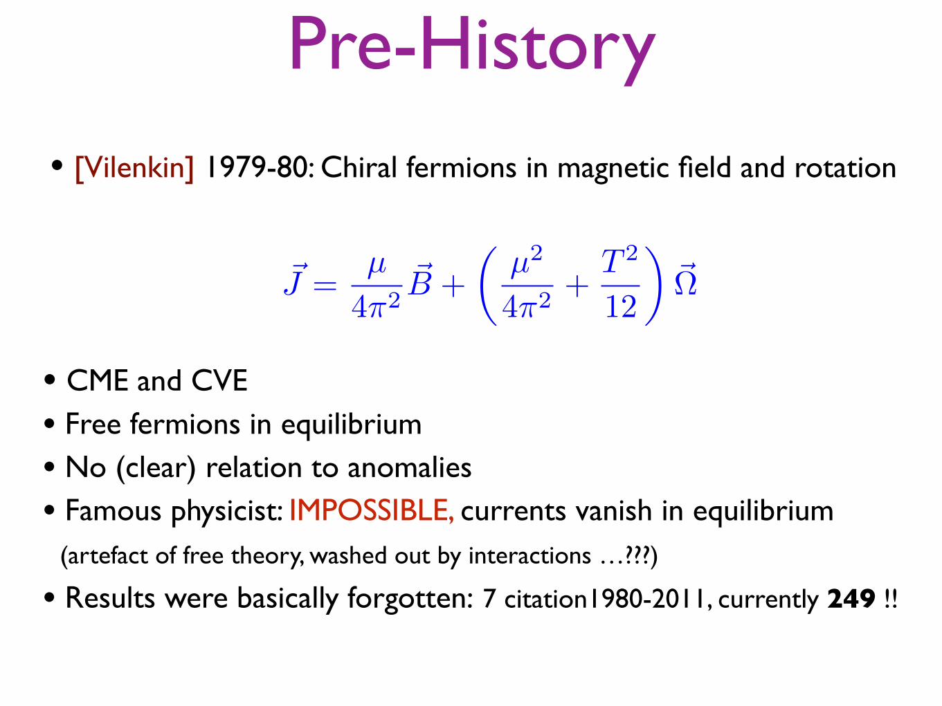
Pre-History• [Vilenkin] 1979-80: Chiral fermions in magnetic field and rotation

~J =µ

4⇡2~B +

✓µ2

4⇡2+

T 2

12

◆~⌦

• CME and CVE

• Free fermions in equilibrium

• No (clear) relation to anomalies

• Famous physicist: IMPOSSIBLE, currents vanish in equilibrium (artefact of free theory, washed out by interactions …???)

• Results were basically forgotten: 7 citation1980-2011, currently 249 !!

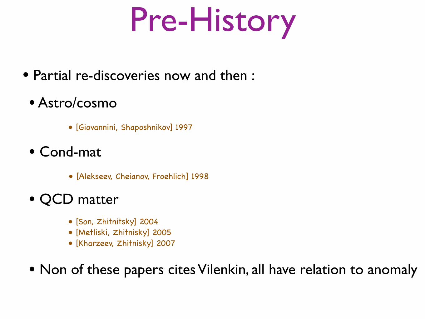
Pre-History• Partial re-discoveries now and then :

• [Giovannini, Shaposhnikov] 1997

• [Son, Zhitnitsky] 2004• [Metliski, Zhitnisky] 2005• [Kharzeev, Zhitnisky] 2007

• [Alekseev, Cheianov, Froehlich] 1998

• Astro/cosmo

• Cond-mat

• QCD matter

• Non of these papers cites Vilenkin, all have relation to anomaly

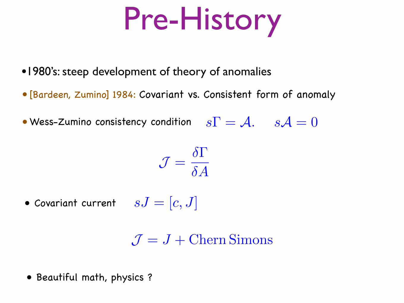
Pre-History•1980’s: steep development of theory of anomalies

• [Bardeen, Zumino] 1984: Covariant vs. Consistent form of anomaly

• Wess-Zumino consistency condition s� = A. sA = 0

J =��

�A

• Covariant current sJ = [c, J ]

• Beautiful math, physics ?

J = J +Chern Simons

History• Precurser 2006: [Newman] “Anomalous Hydrodynamics”

• Sep. 2008: enters Holography [Erdmenger, Haack, Kaminski, Yarom][Banerjee, Bhattacharya, Bhattacharyya, Dutta, Loganayagam, Surowka]

• Study hydrodynamics via fluid/gravity

• Find Chiral Vortical Effect is due to anomaly (Newman: CME due to anomaly)

• Strongly interacting system!

S5D =

3

ZA ^ F ^ F

~⌦ =1

2~r⇥ ~vFluid vorticity:

~J = 8µ2~⌦ =NfNc

4⇡2µ2~⌦

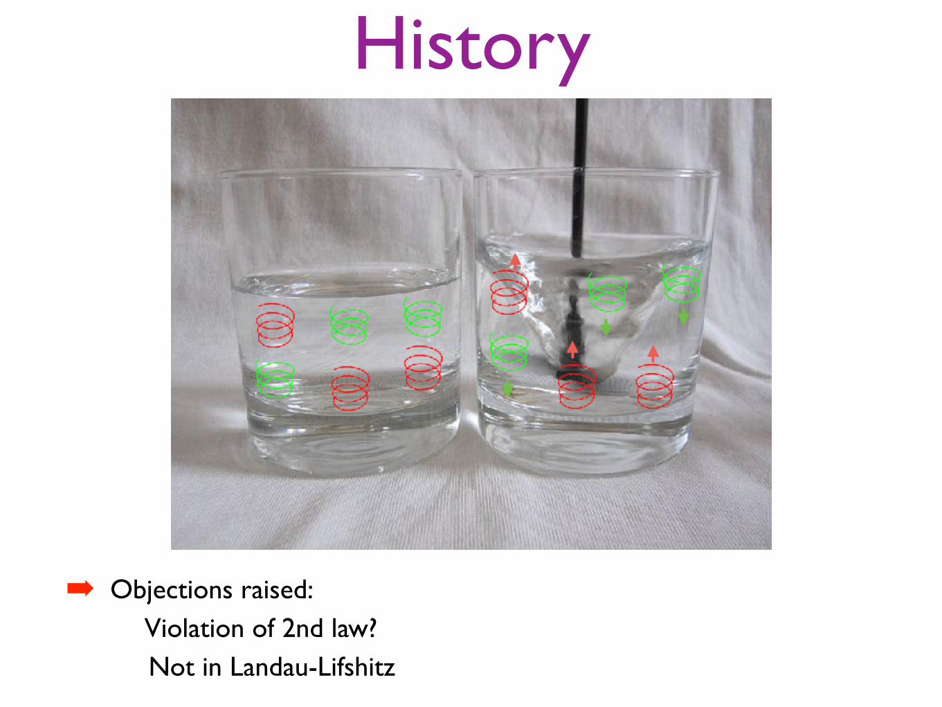
History

➡ Objections raised: Violation of 2nd law? Not in Landau-Lifshitz

History• [Son, Surowka] 2009 “Hydrodynamics with triangle anomalies”

• Combine 2nd law with anomalies

• [Neimann, Oz] 2010 generalisation to non-abelian

@µJµS � 0

⇠B = Cabcµc +

na

✏+ p

✓1

2Cabcµ

cµd + �bT2

◆

Jµ = ⇠BBµ + ⇠V !

µ

(DµJµ)a =

1

8Cabc✏

µ⌫⇢�F bµ⌫F

c⇢�

• Landau frame

• Covariant anomaly

• Undetermined integration constant T^2

History• Aug. 2008: "The Chiral Magnetic Effect” [Fukushima, Kharzeev, Warringa]

~J =µ5

2⇡2~B

B

JE

n- 0 1

• Topology of QCD fields

• CME induces charge separation

• First observable of anomalous transport

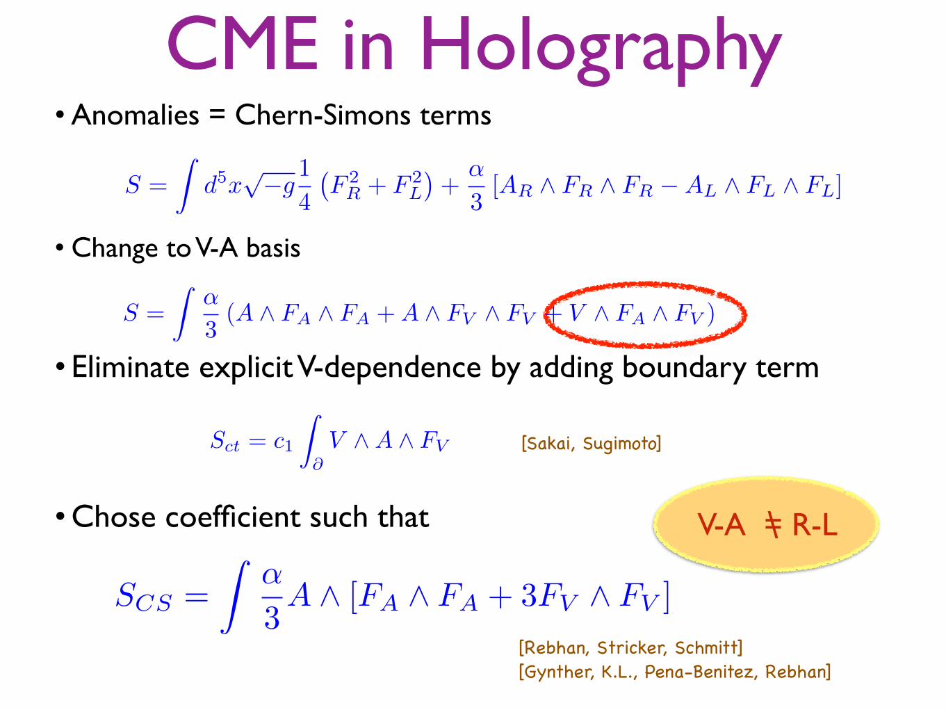
CME in Holography• Anomalies = Chern-Simons terms

• Change to V-A basis

• Eliminate explicit V-dependence by adding boundary term

Sct = c1

Z

@V ^A ^ FV

• Chose coefficient such that

S =

Z↵

3(A ^ FA ^ FA +A ^ FV ^ FV + V ^ FA ^ FV )

S =

Zd5x

p�g

1

4

�F 2R + F 2

L

�+

↵

3[AR ^ FR ^ FR �AL ^ FL ^ FL]

SCS =

Z↵

3A ^ [FA ^ FA + 3FV ^ FV ]

V-A = R-L\

[Rebhan, Stricker, Schmitt][Gynther, K.L., Pena-Benitez, Rebhan]

[Sakai, Sugimoto]

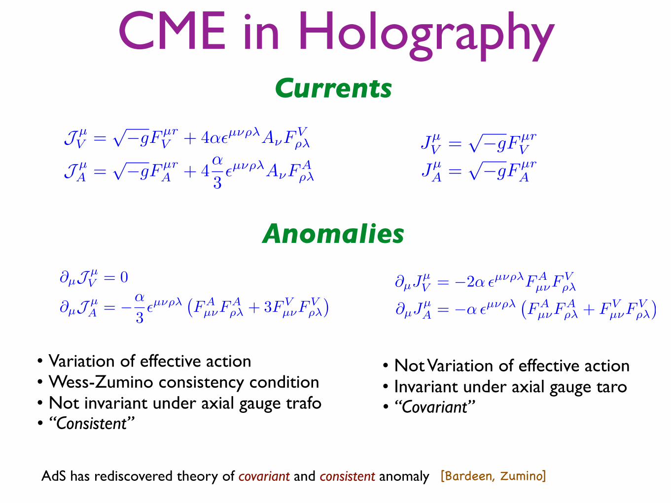
CME in HolographyCurrents

Anomalies

JµV =

p�gFµr

V

JµA =

p�gFµr

A

J µV =

p�gFµr

V + 4↵✏µ⌫⇢�A⌫FV⇢�

J µA =

p�gFµr

A + 4↵

3✏µ⌫⇢�A⌫F

A⇢�

@µJ µV = 0

@µJ µA = �↵

3✏µ⌫⇢�

�FAµ⌫F

A⇢� + 3FV

µ⌫FV⇢�

�@µJ

µV = �2↵ ✏µ⌫⇢�FA

µ⌫FV⇢�

@µJµA = �↵ ✏µ⌫⇢�

�FAµ⌫F

A⇢� + FV

µ⌫FV⇢�

�

• Variation of effective action• Wess-Zumino consistency condition• Not invariant under axial gauge trafo• “Consistent”

• Not Variation of effective action• Invariant under axial gauge taro• “Covariant”

[Bardeen, Zumino]AdS has rediscovered theory of covariant and consistent anomaly

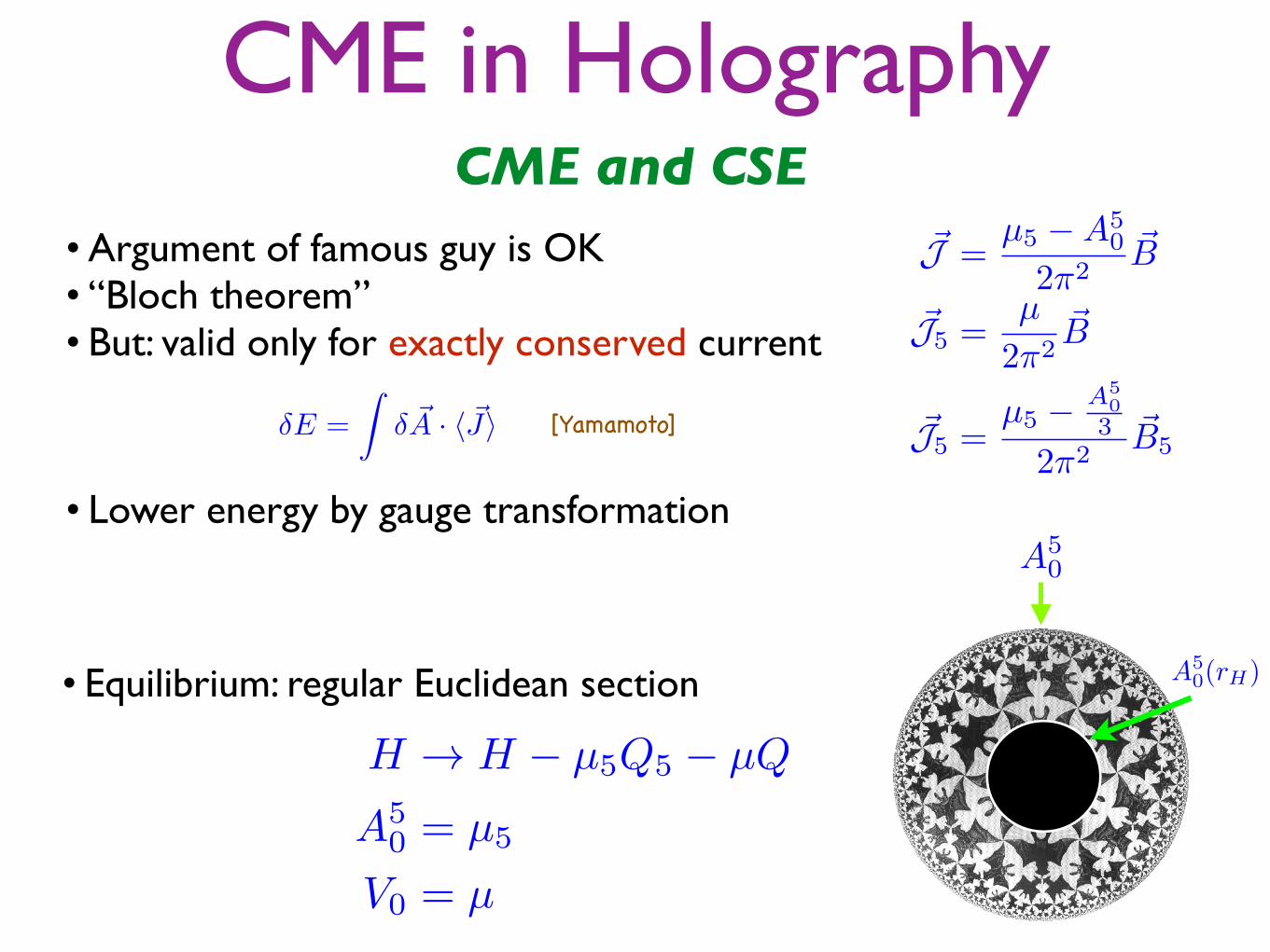
CME in HolographyCME and CSE

~J =µ5 �A5

0

2⇡2~B

~J5 =µ

2⇡2~B

~J5 =µ5 � A5

03

2⇡2~B5

• Equilibrium: regular Euclidean section

H ! H � µ5Q5 � µQ

A50 = µ5

V0 = µ

A50

A50(rH)

• Argument of famous guy is OK• “Bloch theorem”• But: valid only for exactly conserved current

�E =

Z� ~A · h ~Ji

• Lower energy by gauge transformation

[Yamamoto]

Gravitational anomaly• Objection: 4-th order in derivatives, too high

• BUT: AdS has 5-th dimension

DµJµ =

1

768⇡2✏µ⌫⇢�R↵

�µ⌫R�

↵⇢�

Zd5xA ^ tr (R ^R) =

Zd5xA ^ tr

⇣R(4) ^R(4) +A ^D(K ^DK)

⌘

• Is there even in flat space• Vanishes at the boundary• Picks up a contribution from the horizon• Suggest “low energy anomaly” • even in flat space, 2 space time derivatives

Kij ⇡@

@rgij

• BUT: K is covariant tensor w.r.t. to 4-dim spacetime

DµJµ = D(K ^DK)

Quantum Currents from 5D• BUT: at the black hole horizon

ds2 = r2f(r)(�dt2 + 2 �Ad�xdt) + r2d�x2 +dr2

r2f(r)

• Following Hawking

• Current

•NO! not anomaly but quantum current (Luttinger) T 2

12⌃Eg. ⌃Bg = ⌃� ⌃Jq

•The Chiral Vortical Effect (CVE) !!

Quantum Currents from 5D

⇧Jq =b

12T 2⇧�

�⇥⇥T

T⇥⇥� ⇥v

[Megias, Melgar, K.L.,Pena-Benitez][Azayanagi, Loganayagam, Ng, Rodriguez],[Chapman, Neiman, Oz],[Grozdanov, Poovuttikul]hydro+geometry: [Jensen,Loganayagam,Yarom], global anomaly: [Golkar, Sethi]

•Current Jµ =p�gFµr � �

2⇡G✏µ⌫⇢�K�

⌫D⇢K��

[Copetti, Fernandez-Pendas, K.L.]

• Luttinger ~Eg = �~rT

T~Bg = r⇥ ~v

D(K ^DK) / f 0(rh)2 @ ~A

@t(~r⇥ ~A)

D(K ^DK) / 64⇡2T 2 ~Eg · ~Bg

Chiral Vortical Effect~J = 64⇡2�T 2~!

[C. Copetti, J. Fernandez-Pendas]

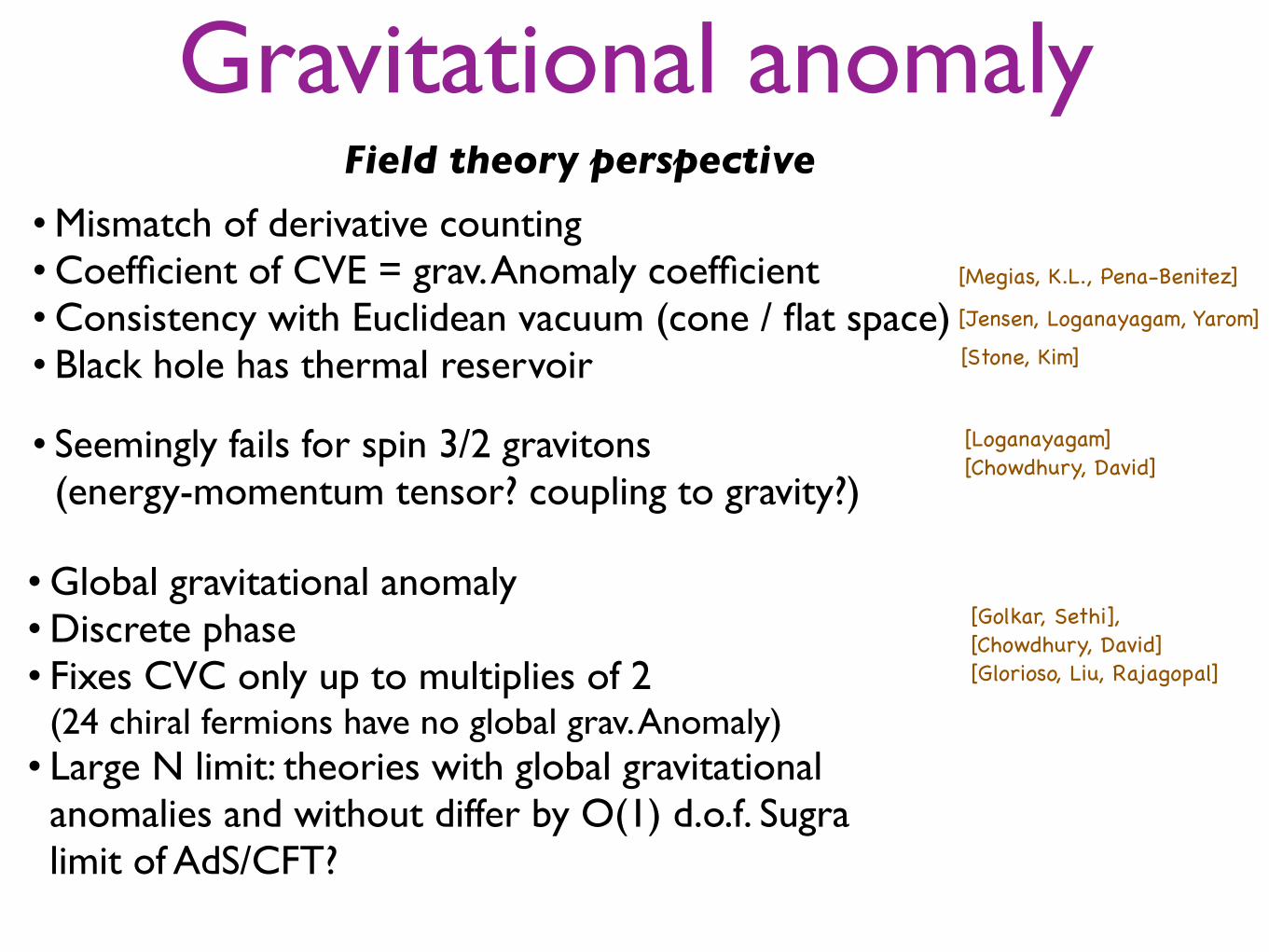
Gravitational anomalyField theory perspective

[Jensen, Loganayagam, Yarom]

• Mismatch of derivative counting• Coefficient of CVE = grav. Anomaly coefficient• Consistency with Euclidean vacuum (cone / flat space)• Black hole has thermal reservoir [Stone, Kim]

• Seemingly fails for spin 3/2 gravitons (energy-momentum tensor? coupling to gravity?)

• Global gravitational anomaly • Discrete phase• Fixes CVC only up to multiplies of 2

(24 chiral fermions have no global grav. Anomaly)• Large N limit: theories with global gravitational anomalies and without differ by O(1) d.o.f. Sugra limit of AdS/CFT?

[Golkar, Sethi], [Chowdhury, David][Glorioso, Liu, Rajagopal]

[Megias, K.L., Pena-Benitez]

[Loganayagam] [Chowdhury, David]

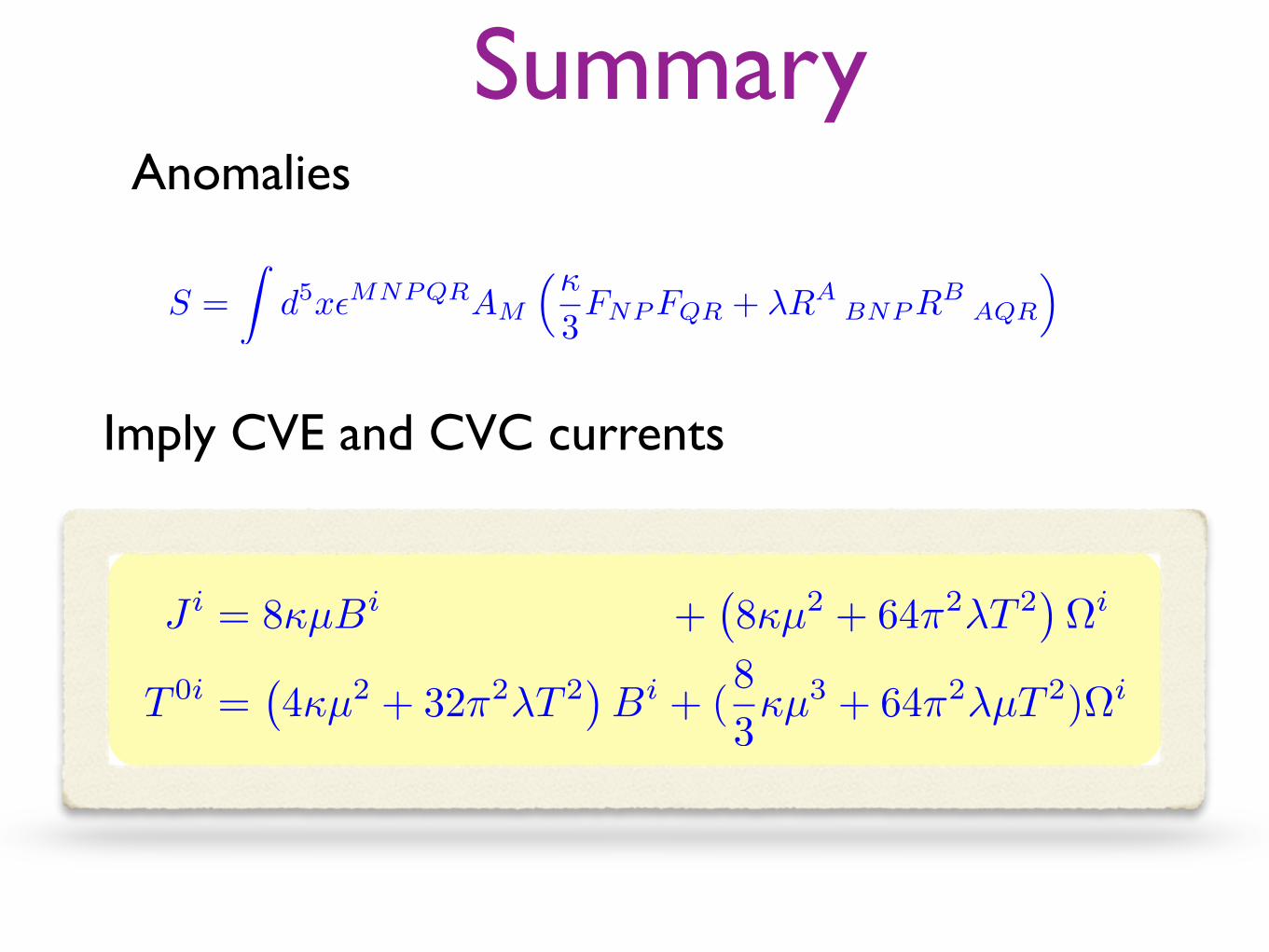
Summary

S =

Zd5x✏MNPQRAM

⇣3FNPFQR + �RA

BNPRB

AQR

⌘

J i = 8µBi +�8µ2 + 64⇡2�T 2

�⌦i

T 0i =�4µ2 + 32⇡2�T 2

�Bi + (

8

3µ3 + 64⇡2�µT 2)⌦i

Anomalies

Imply CVE and CVC currents

3 Examples

I. Breaking the axial symmetry (Mass)

II. Breaking translation symmetry (Impurities)

III. Quenching anomalous transport

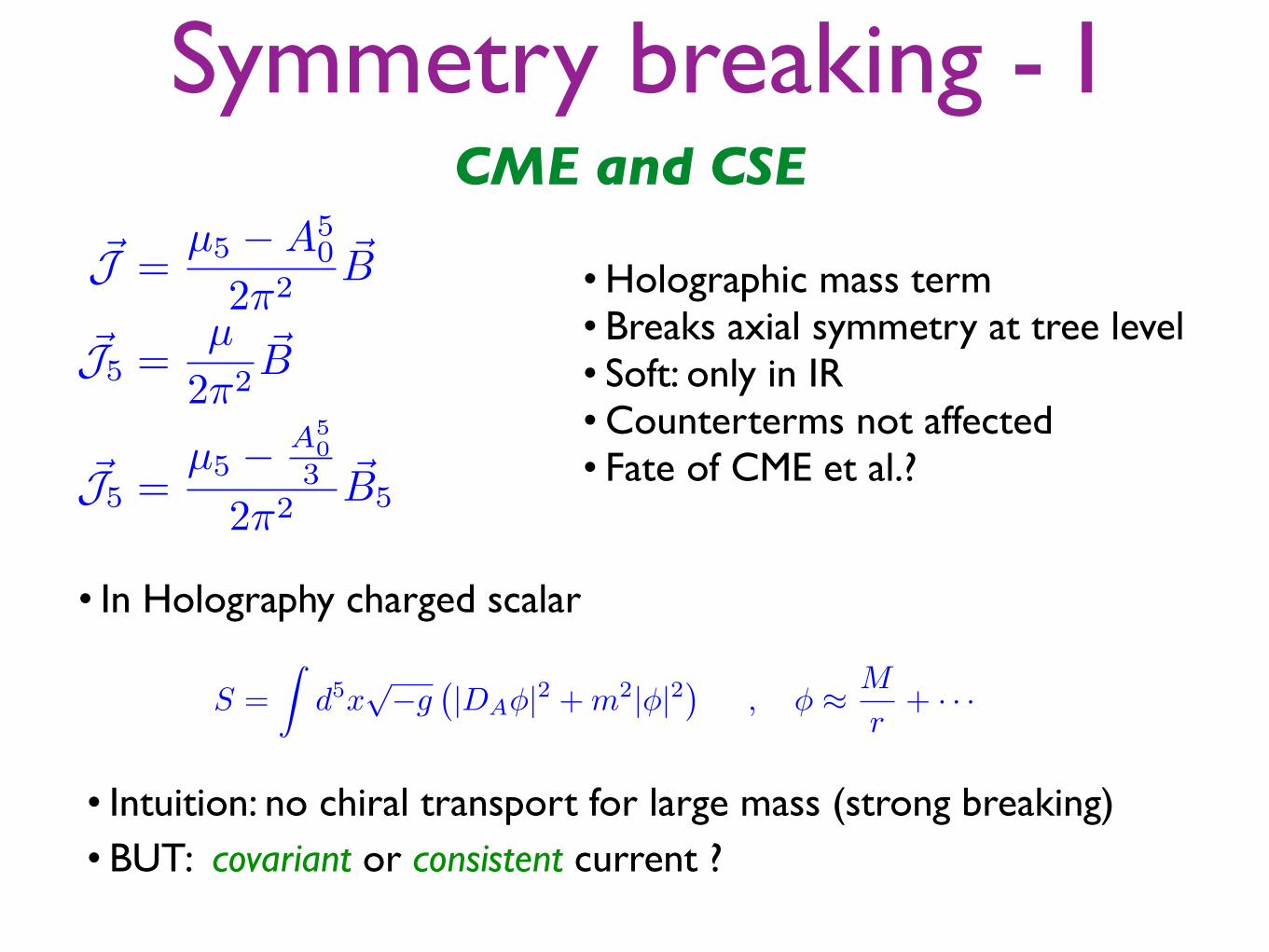
Symmetry breaking - ICME and CSE

~J =µ5 �A5

0

2⇡2~B

~J5 =µ

2⇡2~B

~J5 =µ5 � A5

03

2⇡2~B5

• Holographic mass term• Breaks axial symmetry at tree level• Soft: only in IR• Counterterms not affected• Fate of CME et al.?

• Intuition: no chiral transport for large mass (strong breaking)• BUT: covariant or consistent current ?

• In Holography charged scalar

S =

Zd5x

p�g

�|DA�|2 +m2|�|2

�, � ⇡ M

r+ · · ·

Symmetry breaking - ICME and CSE

in which the axial symmetry is maximally broken the total axial current vanishes! This

seems a very intuitive result.

Finally we consider the case µ5 = 0, µ 6= 0. For simplicity we will discuss the

chiral separation conductivity in the linear response approximation, i.e. with vanishing

background magnetic field. When B = 0, we have a simple solution with non vanishing

fields Vt = µ(1� r20r2 ) and � as the same as (2.18). In this case �B = �55 = 0 while nonzero

�CSE which can be found in the right plot of Fig. 8. Let us make a comment on the

behaviour of the chiral separation conductivity. In this case there is no contribution due

to the Chern-Simons term to the current since we only switch on a chemical potential

for the conserved vector like symmetry µ 6= 0. We find that also in this case the axial

current induced by a magnetic field vanishes in the limit of maximal axial symmetry

breaking. Since in this case there is no Chern-Simons current also the covariant current

vanishes.

0.0 0.2 0.4 0.6 0.8 1.00

2

4

6

8

qM

Μ5

Σ55

ΑΜ5

0 10 20 30 40

0

2

4

6

8

M

T

ΣCSE

ΑΜ

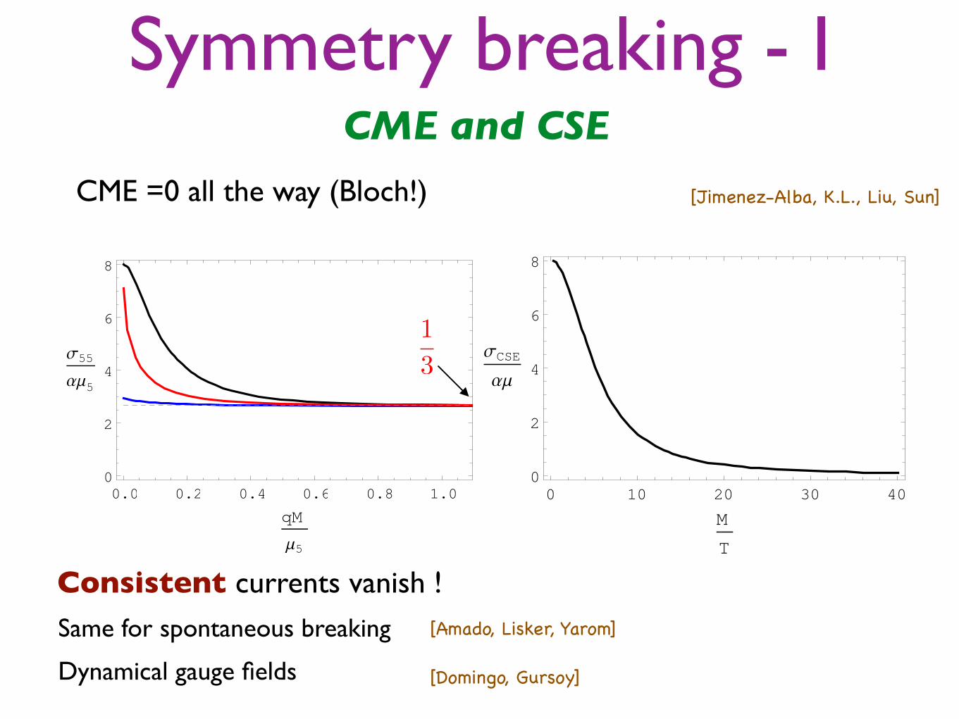
Figure 8: Left plot: �55 as a function of the source M for 8B↵/⇡2T 2 = 0.1,↵ = 1,

T/µ5 = 0.05 (blue), 0.075 (red), 0.1 (black). Note that Tc/µ5 ' 0.765 for this case.

Dashed line �55/(↵µ5) = 8/3. Right plot: �CSE as a function of M/T for B = 0 and

µ5 = 0 while µ 6= 0. When M ! 0, we have �CSE = 8↵µ. For large M , �CSE ! 0.

The important conclusion of this analysis is that in the limit of maximal axial

symmetry breaking via the mass parameterM the expectation value of the axial current

J5 vanishes for both the chiral separation e↵ect and the axial magnetic e↵ect, but only

if one uses the consistent definition of the currents. Since a vanishing axial current for

maximal axial symmetry breaking seems a physically plausible result we take this as

an argument in support of using the consistent definition of currents.

22

CME =0 all the way (Bloch!) [Jimenez-Alba, K.L., Liu, Sun]

Consistent currents vanish !Same for spontaneous breaking [Amado, Lisker, Yarom]

1

3

[Domingo, Gursoy]Dynamical gauge fields

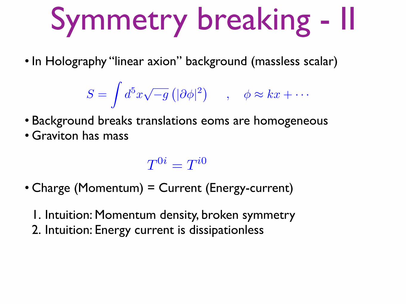
Symmetry breaking - II• In Holography “linear axion” background (massless scalar)

S =

Zd5x

p�g

�|@�|2

�, � ⇡ kx+ · · ·

• Background breaks translations eoms are homogeneous• Graviton has mass

1. Intuition: Momentum density, broken symmetry2. Intuition: Energy current is dissipationless

T 0i = T i0

• Charge (Momentum) = Current (Energy-current)

Symmetry breaking - II• Can extrinsic curvature term be seen in UV?

f = 1� k2

r2� (1� k2

4)r4H

r4ds2 = �fr2dt2 +

dr2

r2f+ r2d~x2

Unusual power!

• Extrinsic curvature as additional variable

�Son�shell =

Z

@

p�g(tµ⌫�gµ⌫ + uµ⌫�Kµ⌫)

• Energy momentum tensor (Ward identity)

⇥µ⌫ = tµ⌫ + uµ�K⌫�

• New term is due to gravitational Chern-Simons term

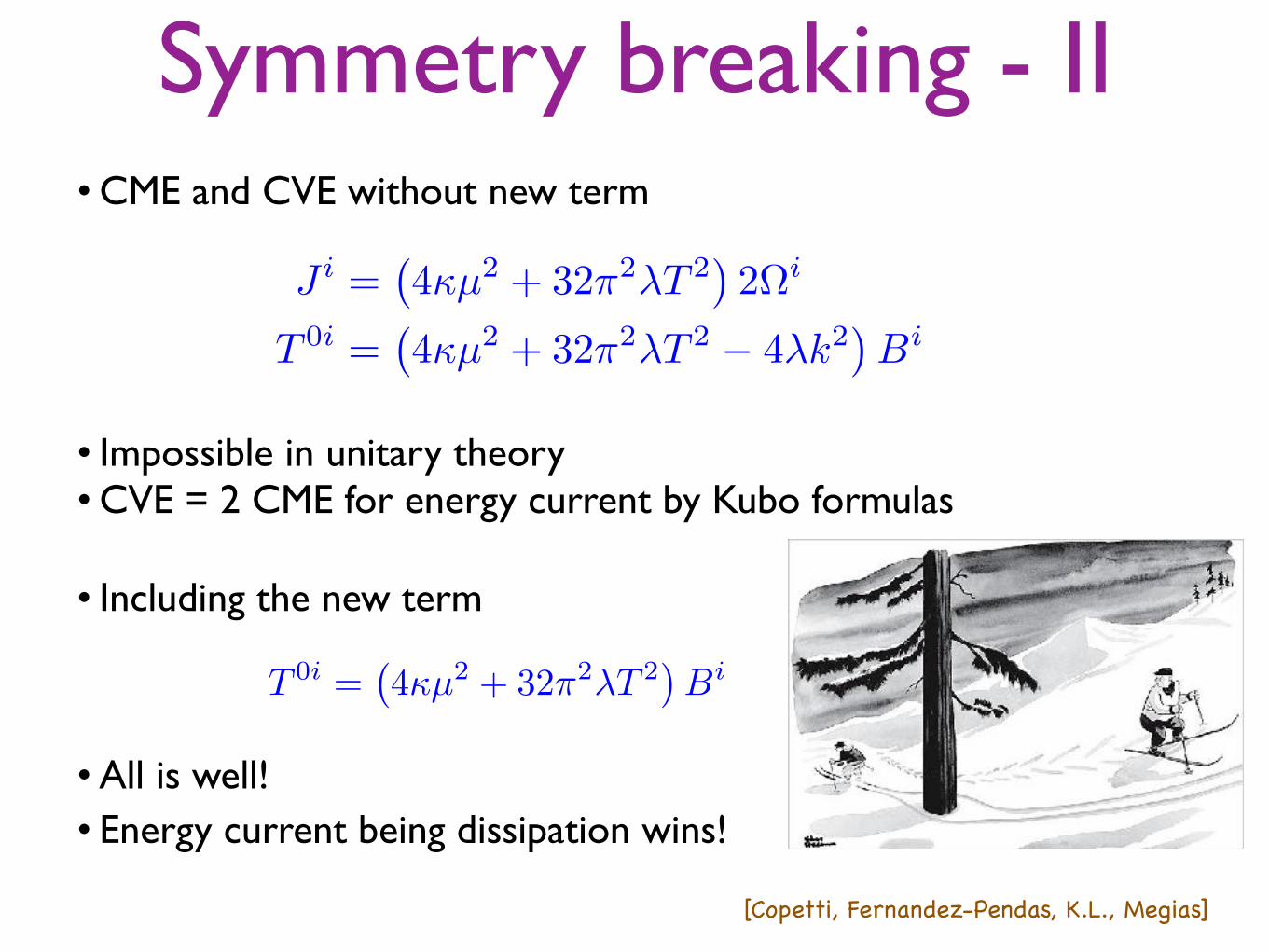
Symmetry breaking - II• CME and CVE without new term

• Impossible in unitary theory• CVE = 2 CME for energy current by Kubo formulas

• Including the new term

• All is well!• Energy current being dissipation wins!

[Copetti, Fernandez-Pendas, K.L., Megias]

J i =�4µ2 + 32⇡2�T 2

�2⌦i

T 0i =�4µ2 + 32⇡2�T 2 � 4�k2

�Bi

T 0i =�4µ2 + 32⇡2�T 2

�Bi

Quenching the CME•CME and CVE depend on equilibrium quantities

•Natural question: anomaly induced transport far from equilibrium physics

• Possible importance for Heavy Ion Collisions (magnetic field has already decayed in hydrodynamic regime)

• Holography allows both: study fast time evolution, quenches and anomalous transport

• Study CME via gravitational Chern-Simons term. ( )

T, µ

T

• “Minimal” setup: inject energy

• Equilibrium: energy — temperature T0 T• CME in energy-momentum tensor• First near equilibrium = hydro

What to look for

Tµ⌫ = (✏+ p)uµu⌫ + p⌘µ⌫ + �̂B(uµB⌫ + u⌫Bµ) ,

Jµ = ⇢uµ + �BBµ ,

JXµ = ⇢Xuµ + �B,XBµ

�̂B = 0

�B = 24↵µ� ⇢

✏+ p

�12↵µ2 + 32�⇡2T 2

�

�B,X = � ⇢X✏+ p

�12↵µ2 + 32�⇡2T 2

�

• Landau frame

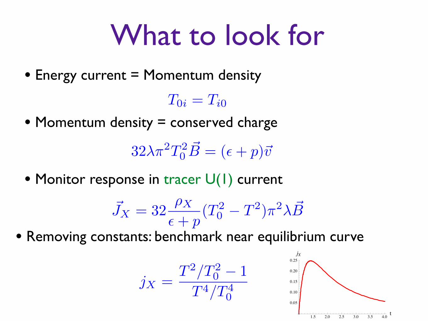
• Energy current = Momentum density

What to look for

T0i = Ti0

• Momentum density = conserved charge

32�⇡2T 20~B = (✏+ p)~v

• Monitor response in tracer U(1) current

~JX = 32⇢X✏+ p

(T 20 � T 2)⇡2�~B

• Removing constants: benchmark near equilibrium curve

jX =T 2/T 2

0 � 1

T 4/T 40

1.5 2.0 2.5 3.0 3.5 4.0t

0.05

0.10

0.15

0.20

0.25jX

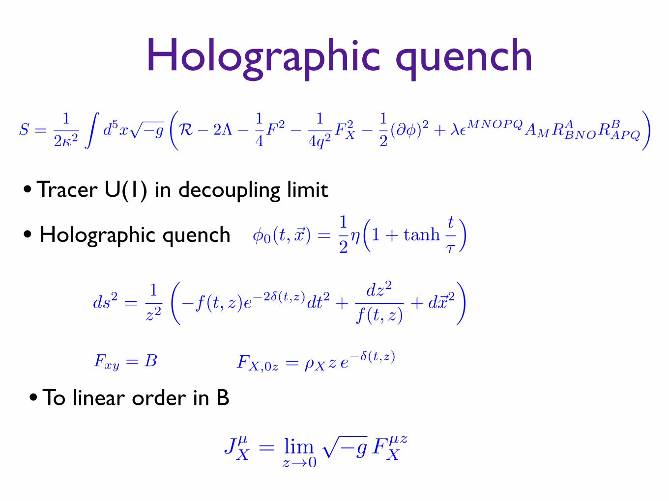
Holographic quenchS =

1

22

Zd5x

p�g

✓R� 2⇤� 1

4F 2 � 1

4q2F 2X� 1

2(@�)2 + �✏MNOPQAMRA

BNORB

APQ

◆

• Tracer U(1) in decoupling limit

• Holographic quench �0(t, ~x) =1

2⌘⇣1 + tanh

t

⌧

⌘

ds2 =1

z2

✓�f(t, z)e�2�(t,z)dt2 +

dz2

f(t, z)+ d~x2

◆

Fxy = B FX,0z = ⇢Xz e��(t,z)

• To linear order in B

JµX = lim

z!0

p�g Fµz

X

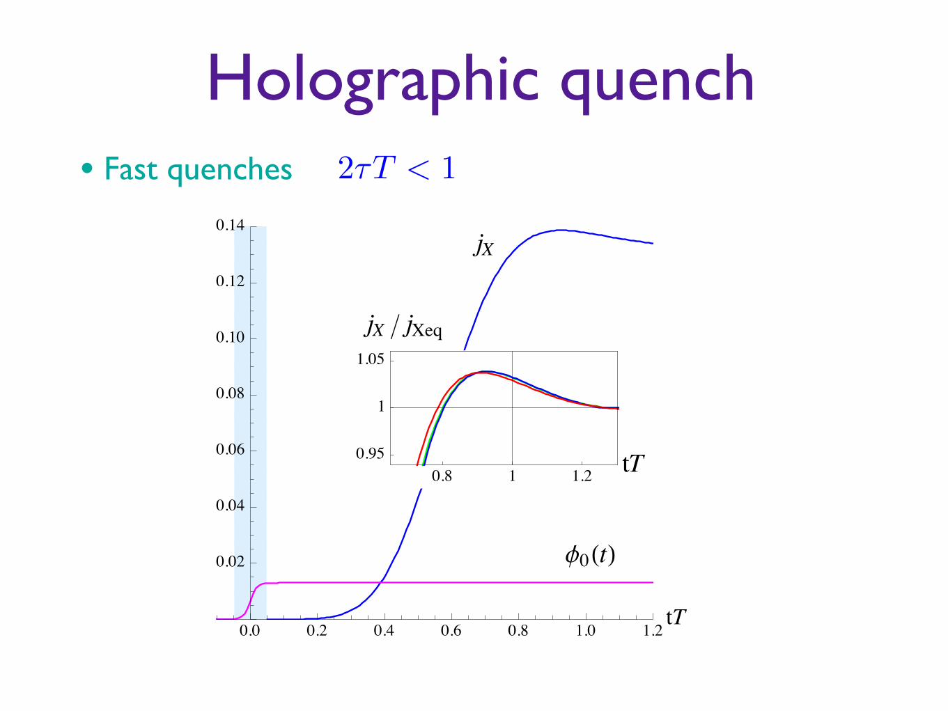
Holographic quench• Fast quenches

jX ë jXeq

0.8 1 1.20.95

1

1.05

tT

f0HtL

jX

0.0 0.2 0.4 0.6 0.8 1.0 1.2tT

0.02

0.04

0.06

0.08

0.10

0.12

0.14

2⌧T < 1

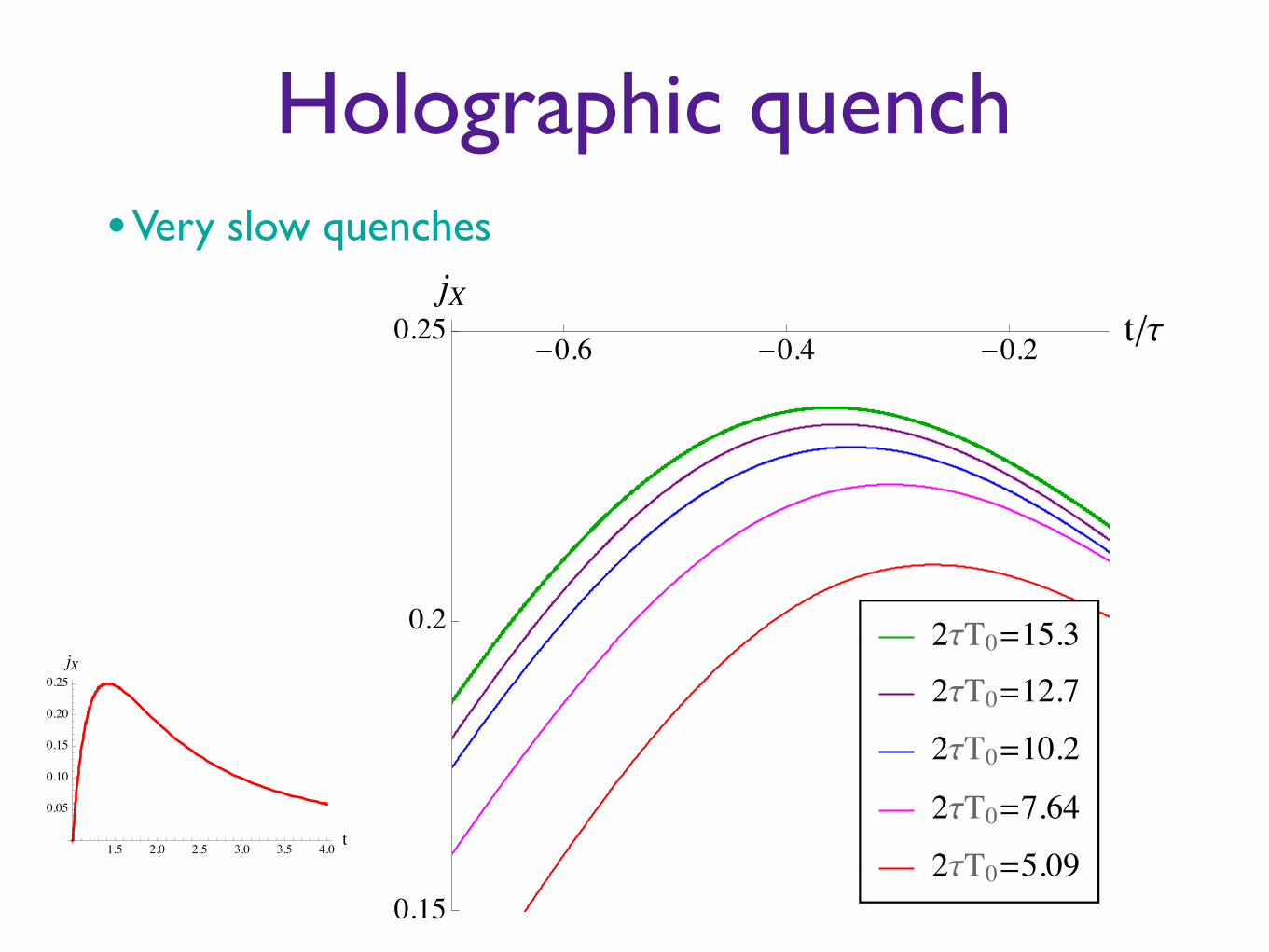
Holographic quench• Very slow quenches

2tT0=15.3

2tT0=12.7

2tT0=10.2

2tT0=7.64

2tT0=5.09

-0.6 -0.4 -0.2 têt

0.15

0.2

0.25jX

1.5 2.0 2.5 3.0 3.5 4.0t

0.05

0.10

0.15

0.20

0.25jX

Cond-Mat applications of anomalous transport theory

WSM

�µ�iDµ + �5A

5µ

� = 0

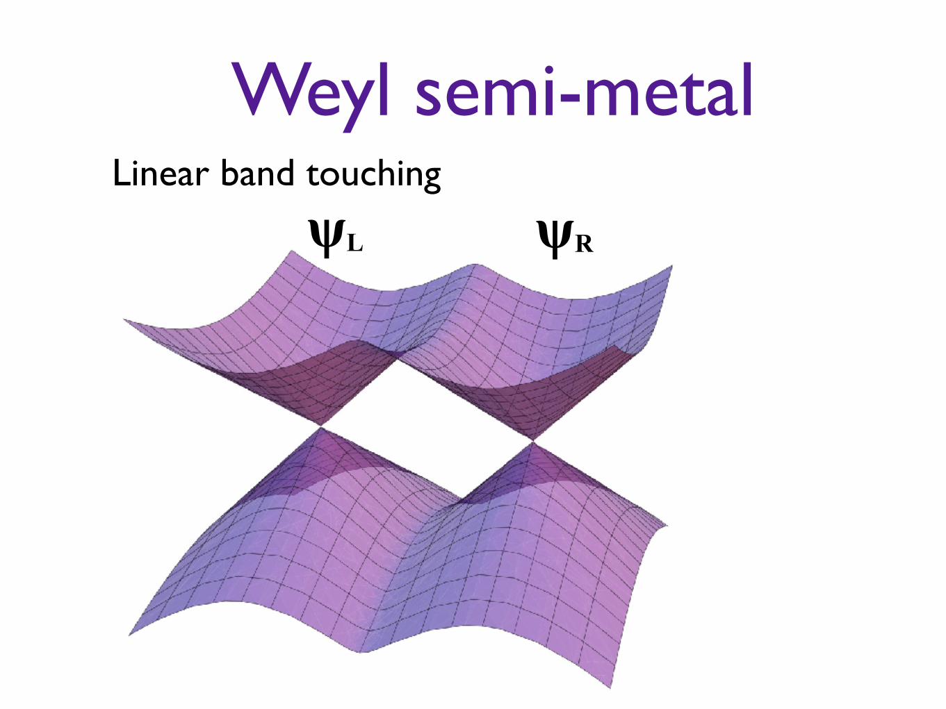
Weyl semi-metalLinear band touching

ψL ψR

Weyl semi-metalTopological constraint (Nielsen-Ninimiya)

Berry connection

Figure 7: B� is defined by removing a small open set U� around each bad point p� in the Brillouinzone.

S⌅n is just⌅n = ±⌅p. (1.22)

This is the identity map, of winding number 1, in the case of + chirality, and it is minusthe identity map, which winds around in reverse, with winding number �1, in the case of �chirality.

The Nielsen-Ninomiya theorem is the statement that the sum of the winding numbers atthe bad points is always 0. Generically (in the absence of lattice symmetries that would leadto a more special behavior) a bad point of winding number bigger than 1 in absolute value willsplit into several bad points of winding number ±1. (We give in section 1.5 an explicit exampleof how this occurs.) So generically, the bad points all have winding numbers ±1, correspondingto gapless Weyl fermions of one chirality or the other. In this case, the vanishing of the sum ofthe winding numbers means that there are equally many gapless modes of positive or negativechirality, as a relativistic field theorist would expect for anomaly cancellation.

How does one prove that the sum of the winding numbers is 0? One rather down-to-earthmethod is as follows. The winding number for a map from S to S⌅n can be expressed as anintegral formula:

w(S) =1

4⇥

⇤d2p �µ⇤⌅n · ⇤µ⌅n⇥ ⇤⇤⌅n. (1.23)

An equivalent way to write the same formula is

w(S) =1

4⇥

⇤

S

d2p �µ⇤ �abcna⇤nb

⇤pµ⇤nc

⇤p⇤. (1.24)

Now0 = ⇤⇥

��⇥µ⇤⌅n · ⇤µ⌅n⇥ ⇤⇤⌅n

⇥, (1.25)

since the right hand side is �⇥µ⇤⇤⇥⌅n · ⇤µ⌅n ⇥ ⇤⇤⌅n, which vanishes because it is the triple crossproduct of three vectors ⇤⇥⌅n, ⇤µ⌅n, and ⇤⇤⌅n that are all normal to the sphere |⌅n| = 1.

For each bad point p�, let U� be a small open ball around p� whose boundary is a sphereS�. Let B be the full Brillouin zone, and let B� be what we get by removing from B all of theU�. Thus the boundary of B� is ⇤B� = ⇤�S� (fig. 7). Then from Stokes’s theorem,

0 =1

4⇥

⇤

B�d3p ⇤⇥

��⇥µ⇤(n · ⇤µn⇥ ⇤⇤n)

⇥

10

BZ has no boundary ! (Torus)

[Witten]

A = ��(k)| ⇥

⇥ki|�(k)⇥dki

FB = dA

dFB = 0

ZdFB

2�=

X

i

I

Ui

FB

2�= 0

[Kiritsis]

(anti-)chiral fermion = (anti-)monopole

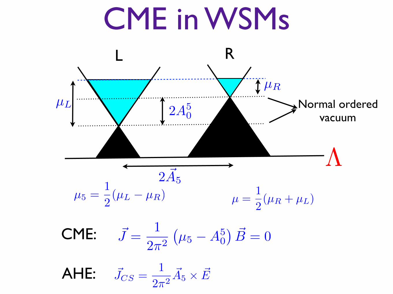
CME in WSMs

⇤

RL

Normal ordered vacuum

µL

µR

µ5 =1

2(µL � µR)

2 �A5

2A50

µ =1

2(µR + µL)

CME: ⇥J =1

2�2

�µ5 �A5

0

�⇥B = 0

AHE: ⇥JCS =1

2�2⇥A5 ⇥ ⇥E

NMR and NTMR in WSM

[J. Zaanen, “Electrons go with the flow in exotic materials”, Science Vol. 351, 6277]

In our holographic calculations, we have not included dissipation e↵ects. It would be

very interesting to test the dissipation e↵ects holographically. Recently there has been a lot of

work in including momentum dissipation in holography. These include the lattice construction

which breaks the translational symmetry explicitly (e.g. [46, 47, 48, 49, 50]) and massive

gravity which breaks the di↵eomorphism symmetry in the bulk (e.g. [51, 52, 53]). Besides

momentum dissipations, we also need to include energy and charge dissipations.

In [30], a bulk massive gauge theory was studied in the chiral anomalous fluid (see also

[54]). The massive gauge theory breaks the U(1) gauge symmetry in the bulk and leads

to charge dissipation for the boundary theory. In a follow up paper, we plan to study the

fluid/gravity analysis of this theory (similar to [8, 9]) to get the charge relaxation time from

the hydrodynamic modes [55].

The holographic energy dissipation e↵ects have not been considered so far. As we argued

in the paper, the holographic zero density system is automatically a system with energy not

conserved for the charge carriers. To encode energy dissipations at finite density, we can as

well mimic the way that momentum dissipations are introduced, such as the Q lattice [49]

or massive gravity constructions [51]. It is possible to combine all the momentum, energy

and charge dissipations holographically to test the formula in this work and we would like to

consider this in future work.

Figure 5: Schematic depiction of an inter valley scattering event. Such an event will lead to axial

charge relaxation. But if the two Weyl cones are at di↵erent chemical potentials (as they are in

parallel external electric and magnetic fields) inter valley scattering will also lead to energy relaxation

since �✏ ⇡ µ5�⇢5.

Finally we would like to point out that in the context of Weyl metals inter-valley scattering

does indeed lead to energy relaxation. A schematic picture of an intervalley scattering event

33

If WSM is not strongly coupled, hierarchy of scattering times

⌧inner < ⌧inter < ⌧ee

Kills Kills Is irrelevant ~P ⇢5, ✏5

NMR and NTMR in WSMNMR = Negative Magnetoresistivity

In equilibrium CME vanishes, Induce non-equilibrium steady state

⇥5 = ⇤5µ5 ⌥J = ⇤ ⌥E +µ5

2⇥2⌥B

⇢̇5 =1

2⇡2( ~E � ~rµ) ~B � 1

⌧5⇢5

~J =

✓� +

⌧5B2

(2⇡2)2�5

◆( ~E � ~rµ)

NTMR via CMECoupled charge and energy transport of chiral currents

GE = ⌧5a2�

det(⌅)

✓@✏

@T� µ

@⇢

@T

◆B2

GT = ⌧52aga�det(⌅)

@⇢

@TB2

Large B (ultraquantum limit):•GE linear in B•GT vanishes

⇢ =|B|4⇡2

µ

[Spivak, Andreev], [Lundgren, Laurell, Fiete] kinetic theory[Lucas, Davison, Sachdev] chiral fluids

~J✏ =⇣a�

2µ2 + agT

2⌘~B

~J = a�µ ~B

~J = GE( ~E � ~rµ) +GT~rT

NMR and NTMR in NbPJohannes Gooth, Anna Corinna Niemann, Tobias Meng, Adolfo G. Grushin, Karl Landsteiner, Bernd Gotsmann, Fabian Menges, Marcus Schmidt, Chandra Shekhar, Vicky Sueß, Ruben Huehne, Bernd Rellinghaus, Claudia Felser, Binghai Yan, Kornelius Nielsch

Experimental signatures of the mixed axial-gravitational anomaly in the Weyl semimetal NbP

arXiv:1703.10682 (Nature)

Angle dependence NMR and NTMR show B2 at small B NMR ~ linear for large B field NTMR vanishes for large B field

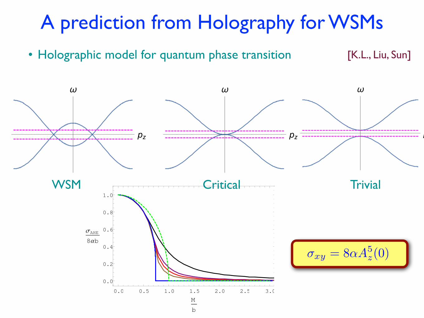
A prediction from Holography for WSMs[K.L., Liu, Sun]

WSM

pz

�

pz

�

pz

�

Critical Trivial

• Holographic model for quantum phase transition

0.0 0.5 1.0 1.5 2.0 2.5 3.0

0.0

0.2

0.4

0.6

0.8

1.0

M

b

ΣAHE

8Αb

⇥xy = 8�A5z(0)

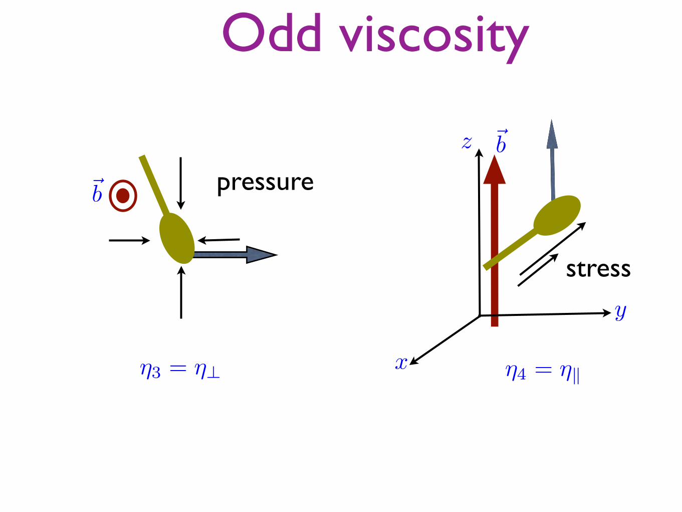
Odd viscosity• Hall viscosity in 2D Quantum Hall states• Time reversal breaking necessary• 2D : invariant e tensor• 3D: need some anisotropy

[Avron, Seiler, Zograf]

[Landau, Lifshytz Vol. 10]

Vij =1

2(@ivj + @jvi)

• In total: 3 shear, 2 “bulk” and 2 odd viscosities

⌧xy = ⌘?Vxy � ⌘H? (Vxx � Vyy)

⌧xz = ⌘kVxz + ⌘Hk Vyz

⌧yz = ⌘kVyz � ⌘Hk Vxz

Odd viscosity

⌘3 = ⌘?

~b

x

y

z

⌘4 = ⌘k

~b

pressure

stress

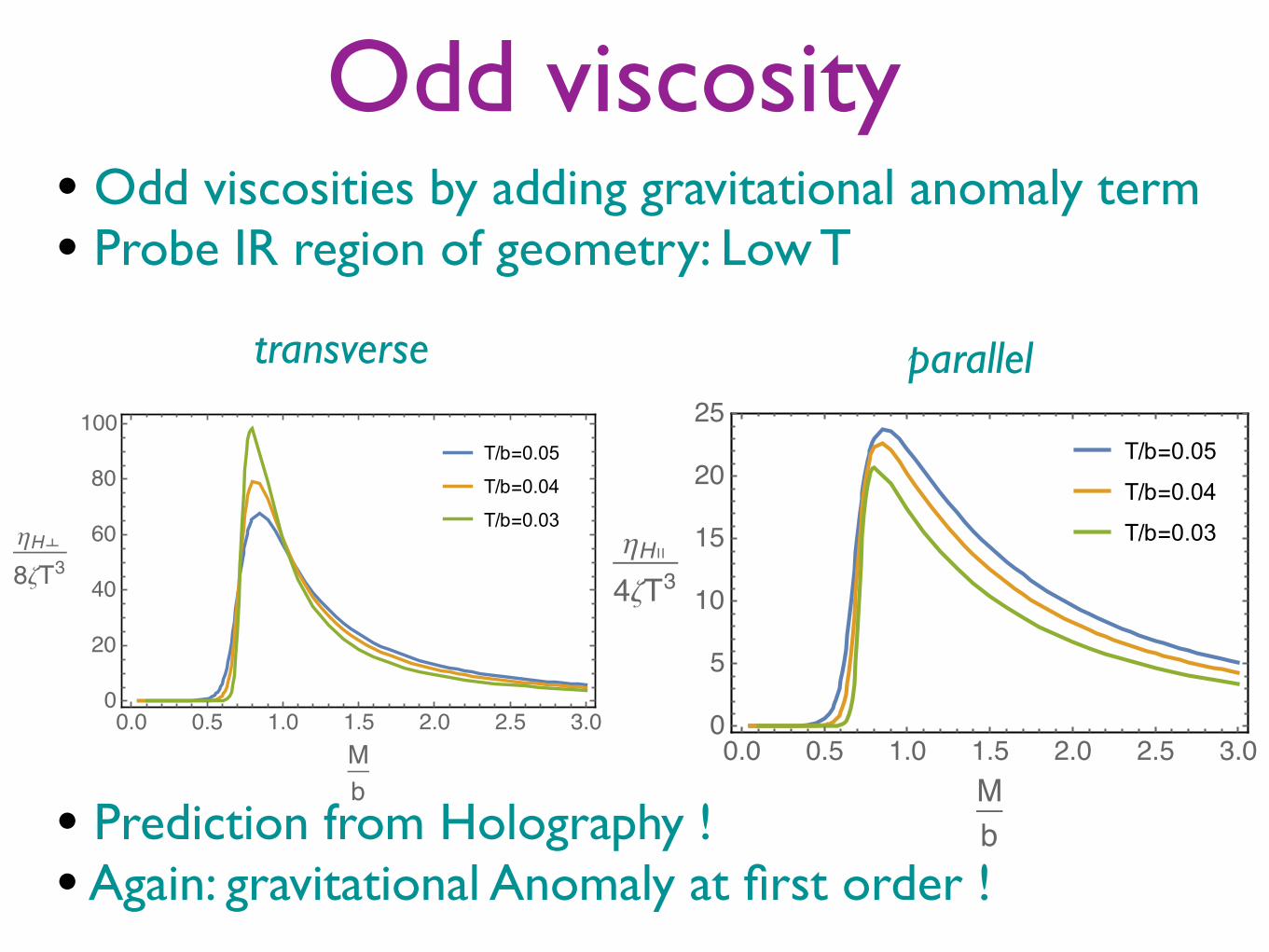
Odd viscosity• Odd viscosities by adding gravitational anomaly term• Probe IR region of geometry: Low T

T/b=0.05T/b=0.04T/b=0.03

��� ��� ��� ��� ��� ��� ����

�

��

��

��

��

��

η�∥

��

transverse

T/b=0.05T/b=0.04T/b=0.03

��� ��� ��� ��� ��� ��� ����

��

��

��

��

���

��

η�⊥�ζ��

parallel

• Prediction from Holography !• Again: gravitational Anomaly at first order !

Summary • Holography is efficient discovery tool for transport • Fate of anomalous transport under symmetry breaking

• New questions:

• Why do consistent currents vanish?

• What is the extrinsic curvature in field theory?

• Anomalous transport far from equilibrium (QGP)

•CME@RHIC vs. CME@LHC