Annulus with Circular Slit Map of Bounded Multiply Connected

BULLETIN of theMALAYSIAN MATHEMATICAL

SCIENCES SOCIETY

http://math.usm.my/bulletin

Bull. Malays. Math. Sci. Soc. (2) 35(4) (2012), 945–959

Annulus with Circular Slit Map of Bounded Multiply ConnectedRegions via Integral Equation Method

1ALI W. K. SANGAWI, 2ALI H. M. MURID AND 3M. M. S. NASSER1 ,2Ibnu Sina Institute for Fundamental Science Studies, Universiti Teknologi Malaysia,

81310 UTM Johor Bahru, Johor, Malaysia1 ,2Department of Mathematics, Faculty of Science, Universiti Teknologi Malaysia,

81310 UTM Johor Bahru, Johor, Malaysia1Department of Mathematics, College of Science, University of Sulaimani, 46001 UOS, Sulaimani, Kurdistan

3Department of Mathematics, Faculty of Science, Ibb University, P. O. Box 70270, Ibb, Yemen3Department of Mathematics, Faculty of Science, King Khalid University, P. O. Box 9004, Abha, Saudi Arabia

[email protected], [email protected], 3mms [email protected]

Abstract. This paper presents a boundary integral equation method for the numerical con-formal mapping of bounded multiply connected region onto an annulus with circular slits.The method is based on some uniquely solvable linear integral equations with classical, ad-joint and generalized Neumann kernels. These boundary integral equations are constructedfrom a boundary relationship that relates the mapping function f on a multiply connectedregion with f ′, θ ′, and | f |, where θ is the boundary correspondence function. Some numer-ical examples are presented to illustrate the efficiency of the presented method.

2010 Mathematics Subject Classification: 30C30, 65E05

Keywords and phrases: Numerical conformal mapping, boundary integral equations, Neu-mann kernel, generalized Neumann kernel, multiply connected regions.

1. Introduction

Conformal mapping is a useful and important tool in science and engineering. On the otherhand, exact mapping functions are unknown except for some special regions. By that fact,the practical use of conformal maps has always been limited. In general conformal mapscannot be obtained in closed form. Thus we have to resort to numerical approximations ofsuch maps. Nowadays, much research has been done to discuss an algorithm for the con-structions of conformal maps. Conformal mapping uses single valued functions of complexvariables to transform a complicated boundary to a simpler, more manageable configuration.Nehari [19, p. 334] described five types of slit regions as important canonical regions forwhich a multiply connected region can be mapped onto. They are the annulus with circularslits, the disk with circular slits, the circular slit region, the radial slit region, and the parallelslit region. Various numerical approximation methods have been proposed for computing

Communicated by V. Ravichandran.Received: September 12, 2011; Revised: December 29, 2011.

946 A. W. K. Sangawi, A. H. M. Murid and M. M. S. Nasser

the conformal map between the multiply connected regions and the five canonical regions;see [1, 3, 5, 6, 8–10, 12–16, 20, 21, 24]. Murid and Mohamed [12] and Mohamed [11, pp.51–88] have discussed a numerical conformal mapping of doubly connected regions ontoan annulus via the Kerzman-Stein and Neumann kernels. Later, Murid and Hu [14] extendthese works to multiply connected regions, which however, involves solving a nonlinearsystem of equation using optimization method. To overcome this nonlinear problem, San-gawi et al. [23] have developed linear integral equations for conformal mapping of boundedmultiply connected regions onto a disk with circular slits. Recently, reformulations of con-formal mappings from the bounded and unbounded multiply connected regions onto the fivecanonical slit regions as Riemann-Hilbert (RH) problems are discussed in Nasser [15–17].An integral equation with the generalized Neumann kernel is then used to solve the RHproblem as developed in [25]. The right-hand side of the integral equation however involvesa singular integral which is computed by Wittich’s method.

In this paper we describe an integral equation method for computing the conformal map-ping function f of multiply connected regions onto an annulus with circular slits. Theapproach presented improves significantly the results of [11–14]. We first derive a bound-ary relationship that relates the mapping function f on a multiply connected region with f ′,θ ′(t), and | f |, where θ is the boundary correspondence function. We then construct threelinear integral equations for f ′, θ ′(t), and | f |. This reduces the nonlinearity problem facedin [8, 14] to linear problem.

The plan of the paper is as follows: Section 2 presents some auxiliary materials andderivations of two integral equations related to f ′. We derive in Section 3 a boundary in-tegral equation satisfied by θ ′. Section 4 presents a method to calculate the modulus of f .Section 5 gives a numerical implementation for computing f based on the computations ofθ ′, modulus of f and f ′(z). In Section 6, we give some examples to illustrate our boundaryintegral equation method. Finally, Section 7 presents a short conclusion.

2. Notations and auxiliary material

Let Ω be a bounded multiply connected region of connectivity M + 1. The boundary Γ

consists of M + 1 smooth Jordan curves Γ0,Γ1, . . . ,ΓM such that Γ1, . . . ,ΓM lies in theinterior of Γ0 , where the outer curve Γ0 has counterclockwise orientation and the in-ner curves Γ1, . . . ,ΓM have clockwise orientation. The positive direction of the contourΓ = Γ0∪Γ1∪ ·· ·∪ΓM is usually that for which Ω is on the left as one traces the boundary(see Figure 1). The curve Γk is parametrized by 2π-periodic twice continuously differen-tiable complex function zk(t) with non-vanishing first derivative, i.e.,

z′k(t) =dzk(t)

dt6= 0, t ∈ Jk = [0,2π] , k = 0,1, . . . ,M.

The total parameter domain J is the disjoint union of M +1 intervals J0, . . . ,JM . We definea parametrization z of the whole boundary Γ on J by

z(t) =

z0(t), t ∈ J0 = [0,2π] ,

...zM(t), t ∈ JM = [0,2π] .

(2.1)

Annulus with Circular Slit Map of Bounded Multiply Connected Regions 947

Let H∗ be the space of all real Holder continuous 2π-periodic functions ω(t) of theparameter t on Jk for k = 0,1, . . . ,M, i.e.

ω(t) =

ω0(t), t ∈ J0,

...ωM(t), t ∈ JM.

Let θ(t) (the boundary corresponding function) be given for t ∈ J by

θ(t) =

θ0(t), t ∈ J0,

...θM(t), t ∈ JM.

Let µ (a picewise constant real function) be given for t ∈ J by

µ(t) = (µ0, . . . ,µM) =

µ0, t ∈ J0,...

µM, t ∈ JM.

The classical Neumann kernel is defined by

N(t,s) =1π

Im(

z′(s)z(s)− z(t)

),

and the adjoint kernel N∗(s, t) of the classical Neumann kernel is given by

N∗(t,s) = N(s, t) =1π

Im(

z′(t)z(t)− z(s)

).

We define the Fredholm integral operators N and N∗ by

Nυ(t) =∫

JN(t,s)υ(s)ds, t ∈ J,

N∗υ(t) =∫

JN∗(t,s)υ(s)ds, t ∈ J.

It is known that λ = 1 is an eigenvalue of the kernel N with multiplicity 1 and λ =−1 is an eigenvalue of the kernel N with multiplicity M [25]. The eigenfunctions of Ncorresponding to the eigenvalue λ =−1 are

χ [1],χ [2], . . . ,χ [M]

, where

χ[ j](ξ ) =

1, ξ ∈ Γ j,0, otherwise, j = 1,2, . . . ,M.

Lastly, we define an integral operator J by

(2.2) Jυ =∫

J

12π

M

∑j=1

χ[ j](s)χ

[ j](t)υ(s)ds,

which is required for uniqueness of solution in a later section.The unit tangent to Γ at z(t) is denoted by T (z(t)) = z′(t)/

∣∣z′(t)∣∣. Suppose that c(z)and Q(z) are complex-valued functions defined on Γ such that Q(z) 6= 0. Then the interiorrelationship is defined as follows:


Figure 1. Mapping of the bounded multiply connected region Ω of connectivity M+1 ontoan annulus with circular slits.

Let P(z) be an analytic function in Ω and satisfies the boundary relationship

P(z) = c(z)T (z)Q(z)

G(z)P(z), z ∈ Γ,(2.3)

where G(z) analytic in Ω, Holder continuous on Γ, and G(z) 6= 0 on Γ. The boundaryrelationship (2.3) also has the following equivalent form:

G(z) = c(z)T (z)Q(z)P(z)2

|P(z)|2, z ∈ Γ.(2.4)

The following theorem from [8] gives an integral equation for an analytic function satisfyingthe boundary relationship (2.3) or (2.4).

Theorem 2.1. Let U and V be any complex-valued functions that are defined on Γ. If thefunction P(z) satisfies the interior non-homogeneous boundary relationship (2.3) or (2.4),then

12

[V (z)+

U(z)T (z)Q(z)

]P(z)+PV

∫Γ

K(z,w)P(w)|dw|

(2.5) +c(z)U(z)

[∑

a j insideΓ

Resw=a j

P(w)(w− z)G(w)

]conj

= 0, z ∈ Γ,

where

(2.6) K(z,w) =1

2πi

[c(z)U(z)

c(w)(w− z)Q(w)− V (z)T (w)

w− z

].

The symbol “conj” in the superscript denotes complex conjugate. The sum in (2.5) is overall those zeros a1,a2, . . . ,aM of G that lie inside Ω. If G has no zeros in Ω, then the termcontaining the residue in (2.5) will not appear.

Let w = f (z) be the analytic function which maps Ω conformally onto an annulus withcircular slits. We assume that a ∈ Ω. The function is made uniquely determined by pre-scribing that f (a) > 0 (see [19, p. 336]). The boundary value of f can be represented in the


form

f (zp(t)) = µpeiθp(t), Γp : z = zp(t), 0≤ t ≤ βp, p = 0,1, . . . ,M,(2.7)

where θp is the boundary correspondence function of Γp. Thus it can be shown that [8]

(2.8) f (zp(t)) =µp

iT (zp(t))

θ′p(t)∣∣θ ′p(t)∣∣ f ′(zp(t))∣∣ f ′(zp(t))

∣∣ , zp ∈ Γp, p = 0,1,2, . . . ,M.

Note that θ′0 > 0, θ

′M < 0, but for p = 1,2, . . . ,M−1, θ

′p may be positive or negative since

each circular slit f (Γp) is traversed twice (see Figure 1). Thus θ′p(t)/

∣∣∣θ ′p(t)∣∣∣= sign(θ′p(t)).

Hence the boundary relationships (2.8) can be written as

(2.9) f (z) = sign(θ′p(t))

| f (z)|i

T (z)f ′(z)| f ′(z)|

, z ∈ Γ.

Comparison of (2.4) and (2.9) leads to a choice of G(z) = f (z), P(z) =√

f ′(z), c(z) =i sign(θ

′p(t)) | f (z)|, Q(z) = 1. Note that since f ′(z) 6= 0 in Ω, a single valued and analytic

branch of√

f ′(z) can be defined. Setting U(z) = T (z)Q(z) and V (z) = 1, Theorem 2.1yields

(2.10)√

f ′(z)+PV∫

Γ

K(z,w)√

f ′(w) |dw|=−c(z)T (z)

×

[∑

a j insideΓ

Resw=a j

√f ′(w)

(w− z) f (w)

]conj

, z ∈ Γ,

where

K(z,w) =1

2πi

[c(z)T (z)

c(w)(w− z)− T (w)

w− z

],

c(z) = i sign(θ′p(t)) | f (z)| , z = z(t),

c(w) = i sign(θ′p(s)) | f (w)| , w = z(s).

Note that f (z) does not have any zeros in Ω. Thus the right-hand side of (2.10) vanishesand the integral equation (2.10) becomes√

f ′(z)+PV∫

Γ

K(z,w)√

f ′(w) |dw|= 0, z ∈ Γ.(2.11)

Our approach here generalizes the results of Murid and Mohamed [12] and Hu [8]. In fact ifΩ is doubly connected then the kernel K(z,w) reduces to the following Kerzman-Stein-typekernel

A∗(z,w) =1

2πi

[| f (z)|T (z)| f (w)|(w− z)

− T (w)w− z

].

Relationship (2.9) is useful for computing the boundary values of the mapping functionf (z) provided θ

′p(t), | f (z)|, and f ′(z) are all known. Note that | f (z0)|= 1, while

∣∣ f (zq)∣∣=

µq, q = 1,2, . . . ,M−1 are the radii of the circular slits and | f (zM)|= µM where µ1, . . . ,µMare undetermined real constants. Another integral equation method for calculating f ′(z) has


been given in Hu [8] and Murid and Hu [14]. They first eliminate the sign(θ′p(t)) in (2.9)

by squaring both sides to get

(2.12) f (z)2 =−| f (z)|2T (z)2 f ′(z)2

| f ′(z)|2, z ∈ Γ.

By means of Theorem 2.1 and (2.12), Murid and Hu [14] formulated the followingboundary integral equation satisfied by f ′(z):

g1(z,a)+∫

Γ

N+(z,w)g1(w,a)|dw|= 0, z ∈ Γ,(2.13)

where

g1(z,a) = T (z) f ′(z),

N+(z,w) =1

2πi

[T (z)z−w

− | f (z)|2T (z)| f (w)|2(z−w)

].

The integral equation (2.13) is similar to the integral equation for finding f ′ in [23] but withdifferent right-hand side. By using single-valuedness of the mapping function f leads to thefollowing condition ∫

−Γq

g1(w,a)|dw|= 0, q = 1,2, . . . ,M.(2.14)

Note that the integral equation (2.13) with the condition (2.14) still are homogeneous. Toovercome this problem we need to find another condition to change the above homogeneousintegral equation to the non-homogeneous integral equation. To achieve this, we divide bothsides of integral equation (2.13) and condition (2.14) by f ′(a), and we obtain

g(z,a)+∫

Γ

N+(z,w)g(w,a)|dw|= 0, z ∈ Γ,(2.15a)

∫−Γq

g(w,a)|dw|= 0, q = 1,2, . . . ,M,(2.15b)

where

g(z,a) =T (z) f ′(z)

f ′(a).

By means of Cauchy’s integral formula we can get the following condition∫Γ

12π

g(w,a)w−a

|dw|= i.(2.15c)

Thus the integral equation (2.15a) with the conditions (2.15b) and (2.15c) should givea unique solution provided the parameters

∣∣ f (zq)∣∣ = µq, q = 1,2, . . . ,M that appear in

N+(z,w) are known.Integral equation methods for computing θ

′p and

∣∣ f (zq)∣∣ = µq are discussed in the next

two sections.


3. Integral equation method for computing θ′p(t)

This section gives another application of Theorem 2.1 for computing f ′/ f . Let f (z) be themapping function as described before. The function f can also be written as

f (z) = (z− z0)eg(z),(3.1)

where a∈Ω, z0 ∈ interior of ΓM, g is an analytic in Ω and α is real constant. It is clear from(2.7) that f ′(zp(t))z′p(t)/ f (zp(t)) = iθ

′p(t). An integral equation method for calculating

f ′(z)/ f (z), z ∈ Γ, is given next. Then the function D(z) defined by

D(z) =f ′(z)f (z)

= g′(z)+1

z− z0,(3.2)

is analytic in Ω.Combining (2.12) and (3.2), we obtain the following boundary relationship

D(z) =−T (z)2

D(z), z ∈ Γ.(3.3)

Comparison of (2.3) and (3.3) leads to a choice of P(z) = D(z), Q(z) = T (z), c(z) =−1,G(z) = 1. Setting U(z) = T (z)Q(z) and V (z) = 1, Theorem 2.1 yields

f ′(z)f (z)

T (z)+PV1

2πi

∫Γ

[T (z)z−w

− T (z)z−w

]f ′(w)f (w)

T (w) |dw|= 0, z ∈ Γ.(3.4)

In the above integral equation let z = z(t) and w = z(s). Then by multiplying both sides of(3.4) by |z′(t)| and using the fact that

f ′(z(t))f (z(t))

z′(t) = iθ ′(t),

the above integral equation can also be written as

θ′(t)+

∫J

N(s, t)θ ′(s)ds = 0.

This integral equation is similar to the integral equation for finding θ ′(t) in [23] but withdifferent right-hand side. Since N(s, t) = N∗(t,s), the integral equation can be written as anintegral equation in operator form

(I+N∗)θ ′ = 0,(3.5)

where λ =−1 is an eigenvalue of N∗ with multiplicity M by Theorem 12 in [25]. By usingthe fundamental theorem [22, p.164] and using the fact that T (w) |dw|= dw, gives∫

−Γp

12π

T (w)f ′(w)f (w)

|dw|=

i, p = M,0, p = 1,2, . . . ,M−1,

(3.6)

which implies that

Jθ′ = (0, . . . ,0,−1).(3.7)

By adding (3.7) to (3.6), we obtain the equation

(I+N∗+J)θ ′ = φ(t),(3.8)

where

φ(t) = (0, . . . ,0,−1).(3.9)

The integral equation (3.8) is uniquely solvable (see [23]).


4. Integral equation for computing | f (z)|

The boundary values of f satisfy on the boundary Γ,

f (z(t)) = µ(t)eiθ(t),(4.1)

where µ(t) = (1,µ1, . . . ,µM).By taking the logarithm on both sides of (3.1), we get

log f (z) = log(z− z0)+g(z).(4.2)

Then

g(z(t)) = lnµ(t)− ln |z(t)− z0|− iarg(z(t)− z0)+ iθ(t)

= γ(t)+h(t)+ iυ ,(4.3)

where γ(t) = −ln |z(t)− z0| and h(t) = lnµ(t) = (0, lnµ1, lnµ2, . . . , lnµM). This choice ofγ(t) is different from the one chosen in [23] which is related to disk with circular slits.

The following theorem gives a method for calculating h(t) and hence µ(t). This theoremcan be proved by using the approach used in proving Theorem 5 in [18].

Theorem 4.1. The function h is given by h = (0,h1,h2, . . . ,hM), where

(4.4) h j = (γ,φ [ j]) =1

2π

∫Jγ(t)φ [ j](t)dt ,

and where φ [ j] is the unique solution of the following integral equation

(4.5) (I+N∗+J)φ [ j] =−χ[ j] , j = 1,2, . . . ,M.

By obtaining h1,h2, . . . ,hM , we obtain

(4.6) µ j = eh j , j = 1,2, . . . ,M.

In summary, by solving the integral equation (3.4) with the condition (3.6) we get θ′p(t).

And solving the integral equation (4.5) we get φ [r], r = 1,2, . . . ,M, which gives hr through(4.4) which in turn gives µr through (4.6). By solving integral equation (2.15a) with the con-ditions (2.15b) and (2.15c) with the known values of µr we get g(z,a). From the definitionof g(z,a), we get

(4.7) f ′(z) =g(z,a) f ′(a)

T (z).

Note that, from the solution of (3.4) and (3.6) it is possible to compute

(4.8)f ′(a)f (a)

=1

2πi

∫Γ

f ′(w)f (w)(w−a)

dw.

Finally from (2.8), (4.7) and (4.8), the boundary value of f (z) is given by

(4.9) f (z) = sign(θ ′(t))| f (z)|

ig(z,a) f ′(a)/ f (a)|g(z,a) f ′(a)/ f (a)|

, z ∈ Γ.

The interior value of the function f (z) is calculated by the Cauchy integral formula

(4.10) f (z) =1

2πi

∫Γ

f (w)w− z

dw, z ∈Ω.


For points z which are not close to the boundary, the integral in (4.10) is approximatedby the trapezoidal rule. However for the points z closed to the boundary Γ, the numericalintegration in (4.10) is nearly singular. This difficulty is overcome by using the fact that(2πi)−1 ∫

Γdw/(w− z) = 1, and rewrite f (z) as

(4.11) f (z) =

∫Γ

f (w)w−z dw∫

Γ

1w−z dw

, z ∈Ω.

This idea has the advantage that the denomenator in this formula compensates for the errorin the numerator (see [7]). The integrals in (4.11) are approximated by the trapezoidal rule.

5. Numerical examples

Since the function zp(t) is 2π-periodic, a reliable procedure for solving the integral equa-tions (2.15), (3.8) and (4.5) numerically is by using the Nystrom’s method with the trape-zoidal rule [2]. The trapezoidal rule is the most accurate method for integrating periodicfunctions numerically [4, pp. 134–142]. Thus solving the integral equations numericallyreduces to solving linear systems of the form

AX = B.(5.1)

The above linear system (5.1) is uniquely solvable for sufficiently large number of colloca-tion points on each boundary component, since the integral equations (2.15), (3.8) and (4.5)are uniquely solvable [2]. The computational details are similar to [15, 23].

For numerical experiments, we have used some test regions of connectivity two, three,four and five based on the examples given in [1, 5, 9, 15, 16, 21, 22]. All the computationswere done using MATHEMATICA 7.1 (16 digit machine precision). The number of pointsused in the discretization of each boundary component Γ j is n. The test regions and theircorresponding images are shown in Figures 2-6.

5.1. Regions of connectivity two

In this section we have used one test region of connectivity two whose exact mapping func-tion is known. The test region is the circular frame. The results for sub norm error betweenthe exact values of f , µ1 and approximate values fn, µ1n are shown in Table 1.

Example 5.1. Circular Frame :Consider a pair of circles

Γ0 : z(t) = eit,Γ1 : z(t) = c+ρe−it, t : 0≤ t ≤ 2π, z0 = 0.3,

such that the domain bounded by Γ0 and Γ1 is the domain between a unit circle and a circlecentered at c with radius ρ [22]. The exact mapping function is given by

(5.2) f (z) =z−λ

λ z−1,

with

λ =2c

1+(c2−ρ2)+√

(1− (c−ρ)2)(1− (c+ρ)2),


which maps Γ0 onto the unit circle and Γ1 onto a circle of radius

µ1 =2ρ

1− (c2−ρ2)+√

(1− (c−ρ)2)(1− (c+ρ)2).

Figure 2 shows the region and its image based on our method. See Table 1 for results.

Out[157]=-1.0 -0.5 0.5 1.0

-1.0

-0.5

0.5

1.0

-1.0 -0.5 0.5 1.0

-1.0

-0.5

0.5

1.0

Figure 2. Conformal mapping of a circular frame onto an annulus.

Table 1. Error Norm (Circular Frame).

n ‖µ1−µ1n‖∞ ‖ f − fn(t)‖∞

4 2.2(−03) 6.5(−02)8 2.2(−05) 1.4(−03)

16 1.9(−09) 2.2(−07)32 8.3(−17) 1.2(−15)

5.2. Regions connectivity three

In this section we have used two test regions of connectivity three whose exact mappingfunctions are unknown. The first test region is bounded by an ellipse and two circles and thesecond test region is bounded by two ellipses and a circle. The results for sub norm errorbetween the our numerical values of µ1, µ2 and the computed values of µ1, µ2 obtainedfrom [5, 9, 15, 16, 21] are shown in Tables 2 and 3.

Example 5.2. Ellipse with Two Circles:Let Ω be the region bounded by

Γ0 : z(t) = 2cos t + i sin t,Γ1 : z(t) = 0.5(cos t− i sin t),Γ2 : z(t) = 1.2+0.3(cos t− i sin t), 0≤ t ≤ 2π.


This example is also discussed in Nasser [16] which allows for comparison of the radii µ1,µ2, where µ1 = 2.3741142722, µ2 = 1.2497448086. Since our condition of the problemis different from him so we should multiply our radii by 2.5 to compare with the result ofNasser [16]. We choose the symbols µ1R and µ2R for the radii in Nasser [16]. Figure 3shows the region and its image based on our method. See Tables 2 for comparison of ourcomputed values of µ1 and µ2 with those computed values of Nasser [16].

Out[119]=-4 -2 2 4

-1.0

-0.5

0.5

1.0

-1.0 -0.5 0.5 1.0

-1.0

-0.5

0.5

1.0

Figure 3. Mapping a region Ω bounded by an ellipse and two circles onto an annulus witha circular slit.

Table 2. Radii comparison for Example 5.2 with [16].

n ‖µ1×2.5−µ1R‖∞ ‖µ2×2.5−µ2R‖∞

32 5.0(−05) 8.9(−04)64 3.8(−07) 8.7(−07)

128 8.6(−13) 1.8(−11)

Example 5.3. Two Ellipses with One Circle:Let Ω be the region bounded by

Γ0 : z(t) = 2cos t + i sin t,Γ1 : z(t) = −0.7+0.25(cos t− i sin t),Γ2 : z(t) = 1+0.5cos t−0.25isin t, 0≤ t ≤ 2π, z0 = 1.

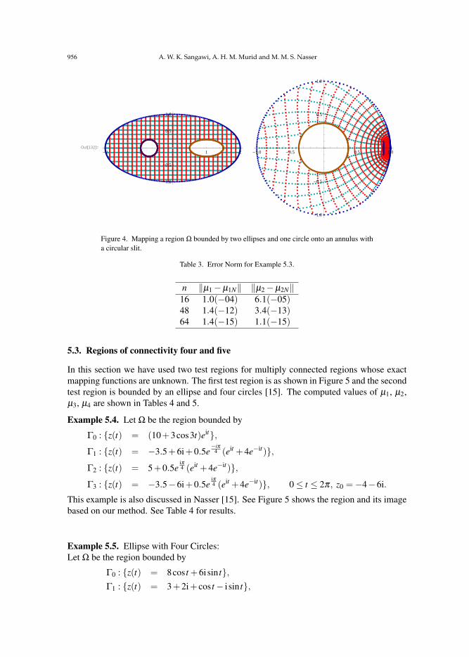
Figure 4 shows the region and its image based on our method. See Table 3 for comparisonbetween our computed values of µ1 and µ2 with those computed values of Nasser [15].


Out[132]=-2 -1 1 2

-1.0

-0.5

0.5

1.0

-1.0 -0.5 0.5 1.0

-1.0

-0.5

0.5

1.0

Figure 4. Mapping a region Ω bounded by two ellipses and one circle onto an annulus witha circular slit.

Table 3. Error Norm for Example 5.3.

n ‖µ1−µ1N‖ ‖µ2−µ2N‖16 1.0(−04) 6.1(−05)48 1.4(−12) 3.4(−13)64 1.4(−15) 1.1(−15)

5.3. Regions of connectivity four and five

In this section we have used two test regions for multiply connected regions whose exactmapping functions are unknown. The first test region is as shown in Figure 5 and the secondtest region is bounded by an ellipse and four circles [15]. The computed values of µ1, µ2,µ3, µ4 are shown in Tables 4 and 5.

Example 5.4. Let Ω be the region bounded by

Γ0 : z(t) = (10+3cos3t)eit,

Γ1 : z(t) = −3.5+6i+0.5e−iπ

4 (eit +4e−it),

Γ2 : z(t) = 5+0.5eiπ4 (eit +4e−it),

Γ3 : z(t) = −3.5−6i+0.5eiπ4 (eit +4e−it), 0≤ t ≤ 2π, z0 =−4−6i.

This example is also discussed in Nasser [15]. See Figure 5 shows the region and its imagebased on our method. See Table 4 for results.

Example 5.5. Ellipse with Four Circles:Let Ω be the region bounded by

Γ0 : z(t) = 8cos t +6isin t,Γ1 : z(t) = 3+2i+ cos t− i sin t,


Out[128]=-5 5 10

-10

-5

5

10

-1.0 -0.5 0.5 1.0

-1.0

-0.5

0.5

1.0

Figure 5. Mapping a region Ω onto an annulus with two circular slits.

Table 4. The numerical values of µ1, µ2 and µ3.

n µ1 µ2 µ332 0.9400798851906385 0.8899301609674942 0.315545695853630864 0.9400786116038745 0.8899315928064306 0.3155455847860195

128 0.940078611605828 0.8899315927710835 0.3155455847853972

Γ2 : z(t) = −3+2i+ cos t− i sin t,Γ3 : z(t) = −3−2i+ cos t− i sin t,Γ4 : z(t) = 3−2i+ cos t− i sin t, 0≤ t ≤ 2π, z0 =−3−2i.

This example is also discussed in Nasser [15]. Figure 6 shows the region and its imagebased on our method. See Table 5 for results.

Table 5. The numerical values of µ1, µ2, µ3 and µ4.

n µ1 µ2 µ3 µ432 0.84922711665091 0.63729798437032 0.210432179308122 0.8074212827774564 0.84922717271639 0.6372980012645 0.210432177445509 0.80742132924948

128 0.84922717271638 0.63729800126452 0.210432177445504 0.80742132924948


Out[135]=-5 5

-6

-4

-2

2

4

6

-1.0 -0.5 0.5 1.0

-1.0

-0.5

0.5

1.0

Figure 6. Mapping a region Ω bounded by an ellipse and four circles onto an annulus withthree circular slits.

6. Conclusion

In this paper, we have constructed new boundary integral equation method for conformalmapping of multiply connected regions onto an annulus with circular slits. We have alsoconstructed a new method to find the values of circular radii that reduces the nonlinearityproblem encountered in Murid and Hu [8] to linear problem. By solving the integral equa-tions, we obtains the values of θ ′, | f | and f ′ which in turn gives the approximate boundaryvalue of the mapping function. These integral equations are similar to the integral equationsin [23] for disk with circular slits but with different right-hand sides. Furthermore the right-hand sides of the integral equations do not involve any singularity. The interior mappingfunction are calculated by the means of the Cauchy integral formula. Several mappings ofthe test regions of connectivity two, three, four and five were computed numerically usingthe proposed method. The numerical examples presented have illustrated that our boundaryintegral equation method has high accuracy.

Acknowledgement. This work was supported in part by the Malaysian Ministry of HigherEducation (MOHE) through the Research Management Centre (RMC), Universiti TeknologiMalaysia (FRGS Votes 78346, 78479). This support is gratefully acknowledged. We wishto thank an anonymous referee for valuable comments and suggestions on the manuscriptwhich improve the presentation of the paper.

References[1] K. Amano, A charge simulation method for the numerical conformal mapping of interior, exterior and doubly-

connected domains, J. Comput. Appl. Math. 53 (1994), no. 3, 353–370.[2] K. E. Atkinson, The Numerical Solution of Integral Equations of the Second Kind, Cambridge Monographs

on Applied and Computational Mathematics, 4, Cambridge Univ. Press, Cambridge, 1997.[3] D. Crowdy and J. Marshall, Conformal mappings between canonical multiply connected domains, Comput.

Methods Funct. Theory 6 (2006), no. 1, 59–76.[4] P. J. Davis and P. Rabinowitz, Methods of Numerical Integration, second edition, Computer Science and

Applied Mathematics, Academic Press, Orlando, FL, 1984.


[5] S. W. Ellacott, On the approximate conformal mapping of multiply connected domains, Numer. Math. 33(1979), no. 4, 437–446.

[6] P. Henrici, Applied and Computational Complex Analysis, Wiley-Interscience, New York, 1974.[7] J. Helsing and R. Ojala, On the evaluation of layer potentials close to their sources, J. Comput. Phys. 227

(2008), no. 5, 2899–2921.[8] L. Hu, Boundary Integral Equations Approach for Numerical Conformal Mapping of Multiply Connected

Regions, PhD Thesis, Department of Mathematics, Universiti Teknologi Malaysia, 2009.[9] C. A. Kokkinos, N. Papamichael and A. B. Sideridis, An orthonormalization method for the approximate

conformal mapping of multiply-connected domains, IMA J. Numer. Anal. 10 (1990), no. 3, 343–359.[10] P. K. Kythe, Computational Conformal Mapping, Birkhauser Boston, Boston, MA, 1998.[11] N. A. Mohamed, An Integral Equation Method for Conformal Mapping of Doubly Connected Regions via the

Kerzman-Stein and the Neumann Kernels, Master Thesis, Department of Mathematics, Universiti TeknologiMalaysia, 2007.

[12] A. H. M. Murid and N. A. Mohamed, Numerical conformal mapping of doubly connected regions via theKerzman-Stein kernel, Int. J. Pure Appl. Math. 36 (2007), no. 2, 229–250.

[13] A. H. M. Murid and M. R .M. Razali, An integral equation method for conformal mapping of doubly con-nected regions, Matematika 15 (1999), no. 2, 79–93.

[14] A. H. M. Murid and L.-N. Hu, Numerical conformal mapping of bounded multiply connected regions by anintegral equation method, Int. J. Contemp. Math. Sci. 4 (2009), no. 21–24, 1121–1147.

[15] M. M. S. Nasser, A boundary integral equation for conformal mapping of bounded multiply connected re-gions, Comput. Methods Funct. Theory 9 (2009), no. 1, 127–143.

[16] M. M. S. Nasser, Numerical conformal mapping via a boundary integral equation with the generalized Neu-mann kernel, SIAM J. Sci. Comput. 31 (2009), no. 3, 1695–1715.

[17] M. M. S. Nasser, Numerical conformal mapping of multiply connected regions onto the second, third andfourth categories of Koebe’s canonical slit domains, J. Math. Anal. Appl. 382 (2011), no. 1, 47–56.

[18] M. M. S. Nasser, A. H. M. Murid, M. Ismail and E. M. A. Alejaily, Boundary integral equations with thegeneralized Neumann kernel for Laplace’s equation in multiply connected regions, Appl. Math. Comput. 217(2011), no. 9, 4710–4727.

[19] Z. Nehari, Conformal Mapping, McGraw-Hill, Inc., New York, Toronto, London, 1952.[20] D. Okano, H. Ogata, K. Amano and M. Sugihara, Numerical conformal mappings of bounded multiply

connected domains by the charge simulation method, J. Comput. Appl. Math. 159 (2003), no. 1, 109–117.[21] L. Reichel, A fast method for solving certain integral equations of the first kind with application to conformal

mapping, J. Comput. Appl. Math. 14 (1986), no. 1–2, 125–142.[22] E. B. Saff and A. D. Snider, Fundamentals of Complex Analysis, Pearson Education, Inc. New Jersey, 2003.[23] A. W. K. Sangawi, A. H. M. Murid and M. M. S. Nasser, Linear integral equations for conformal mapping of

bounded multiply connected regions onto a disk with circular slits, Appl. Math. Comput. 218 (2011), no. 5,2055–2068.

[24] G. T. Symm, Conformal mapping of doubly-connected domains, Numer. Math. 13 (1969), 448–457.[25] R. Wegmann and M. M. S. Nasser, The Riemann-Hilbert problem and the generalized Neumann kernel on

multiply connected regions, J. Comput. Appl. Math. 214 (2008), no. 1, 36–57.

Annulus with Circular Slit Map of Bounded Multiply Connected

Documents

Transcript of Annulus with Circular Slit Map of Bounded Multiply Connected