ANNOTATED OUTPUT--SPSS Descriptive Statistics · 2013-12-20 · SPSS considers these values...

ANNOTATED OUTPUT--SPSS

Center for Family and Demographic Research http://www.bgsu.edu/organizations/cfdr/index.html Updated 5/25/2006

Descriptive Statistics DESCRIPTIVES VARIABLES=age attend happy married racenew male sexfreq /STATISTICS=MEAN STDDEV MIN MAX .

Descriptive Statistics

2751 18 89 46.28 17.3702743 0 8 3.66 2.7021369 1 3 1.82 .6292765 0 1 .46 .4982762 0 1 .76 .4282765 0 1 .44 .497

2151 0 6 2.83 2.013

1052

AGECHURCH ATTENDANCEGENERAL HAPPINESSMARITAL (Married =1)RACE (White =1)GENDER (Male =1)FREQUENCY OF SEXDURING LAST YEARValid N (listwise)

N Minimum Maximum Mean Std. Deviation

“N” = The number of cases with valid responses for each variable. For general happiness there are 1369 valid responses. “Minimum” = The minimum possible value for each variable. Recall that values for general happiness are coded (1) very happy, (2) pretty happy, and (3) not too happy. “Maximum” = The maximum possible value for each variable.

“Valid N” = This value indicates the number of cases with valid responses for all variables listed above.

“Mean” = The mean value for all 2751 cases. Respondents have a mean age of 46.28 years. “Std. Deviation” = The standard deviation is a measure of dispersion around the mean. For example, the mean age for this sample is 46, with a standard deviation of 17. So, 95% of the cases in a normal distribution will be between 29 and 63.

Since we have coded race, gender, marital status as dummies, the means can be interpreted as the percent of respondents reporting the focus category (1=male, 1=white, 1=married). For gender, 44% of the respondents are male. For race, 76% of the respondents are white. For marital status, 46% of the respondents are



Frequencies FREQUENCIES VARIABLES=happy /ORDER= ANALYSIS .

GENERAL HAPPINESS

415 15.0 30.3 30.3784 28.4 57.3 87.6170 6.1 12.4 100.0

1369 49.5 100.01393 50.4

1 .02 .1

1396 50.52765 100.0

VERY HAPPY (1)PRETTY HAPPY (2)NOT TOO HAPPY (3)Total

Valid

NAP (0)DK (8)NA (9)Total

Missing

Total

Frequency Percent Valid PercentCumulative

Percent

The missing values for this variable include values 0, 8, and 9. SPSS considers these values “system missing” and therefore they are not included in analyses. For this example, 50.5% of the total cases are “system missing,” with a vast majority classified as “NAP” or not applicable. “NAP” typically refers to respondents who skipped out of the question.

The percent column indicates simply the percentage of cases in each of the groups. In this example, 15.0% of the cases have a value of (1) very happy. This column includes all possible values, including system missing values.

The valid percent column includes only cases that are not classified as “system missing.” For this example, of the valid responses, 30.3% of the cases have a value of (1) very happy. Notice the differences between the percent and valid percent columns.



Correlations The correlation tells you the magnitude and direction of the association between two variables. CORRELATIONS /VARIABLES=happy sexfreq age /PRINT=TWOTAIL NOSIG /MISSING=PAIRWISE .

Correlations

1 -.105** -.045. .001 .094

1369 1060 1362-.105** 1 -.437**.001 . .000

1060 2151 2143-.045 -.437** 1.094 .000 .

1362 2143 2751

Pearson CorrelationSig. (2-tailed)NPearson CorrelationSig. (2-tailed)NPearson CorrelationSig. (2-tailed)N

GENERAL HAPPINESS

FREQUENCY OF SEXDURING LAST YEAR

AGE OF RESPONDENT

GENERALHAPPINESS

FREQUENCYOF SEXDURING

LAST YEAR

AGE OFRESPON

DENT

Correlation is significant at the 0.01 level (2-tailed).**.

Note The following general categories indicate a quick way of interpreting correlations. 0.0 – 0.2 Very weak correlation 0.2 – 0.4 Weak correlation 0.4 – 0.7 Moderate correlation 0.7 – 0.9 Strong correlation 0.9 – 1.0 Very strong correlation

This cell represents the correlation (and significance and sample size) between age and general happiness. The top value (-.045) is the correlation coefficient. The middle value (.094) is the significance level. The bottom value (1362) is the number of cases. In this example, the correlation is not significant at the p < .05 level.

Here is the correlation between age of respondent and frequency of sex. The correlation coefficient is -.437 (and is significant). This suggests a negative correlation with moderate magnitude. As age increases, the frequency of sex decreases. The correlation between age and frequency of sex is -.437. If we square this value, we get .190969, or 19.1 out of 100, or 19.1 percent. From this we can claim that roughly 19.1% of the variation in frequency of sex is attributed to respondent’s age.



T-Tests The Independent Sample T-Test compares the mean scores of two groups on a given variable. In this example, we compare “frequency of sex” for males versus females. Null Hypothesis: The means of the two groups (males and females) are not significantly different. Alternate Hypothesis: The means of the two groups (males and females) are significantly different. T-TEST GROUPS = Male(0 1) /MISSING = ANALYSIS /VARIABLES = sexfreq /CRITERIA = CI(.95) .

Group Statistics

976 3.10 1.912 .0611175 2.60 2.067 .060

RESPONDENT'S SEXMALEFEMALE


N Mean Std. DeviationStd. Error

Mean

We can see here that males report higher frequencies of sex than females. However, we cannot tell from here whether or not this difference is significant.



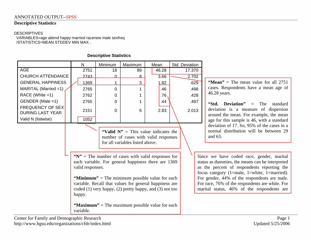
Independent Samples Test

31.470 .000 5.800 2149 .000 .50 .087 .332 .672

5.842 2124.146 .000 .50 .086 .333 .670

Equal variancesassumedEqual variancesnot assumed


F Sig.

Levene's Test forEquality of Variances

t df Sig. (2-tailed)Mean

DifferenceStd. ErrorDifference Lower Upper

95% ConfidenceInterval of the

Difference

t-test for Equality of Means

If Levene’s Test was significant (variances are different), then read the bottom line. If Levene’s Test is not significant (variances are equal), then read the top line. In this example, we read the bottom line. Our “t” value is 5.842, with 2124 degrees of freedom. There is a significant difference between the two groups. We can conclude, then, that males and females significantly differ in their reports of sexual frequency: males reported higher levels of sexual frequency than did females. The circled value indicates the difference in means (male score minus female score).

Levene’s Test tells us if we have met the assumption that the two groups have approximately equal variances on the dependent variable. If Levene’s Test is significant (“Sig.” is less than .05), the two variances are significantly different. If Levene’s Test is not significant, then the two variances are approximately equal, and the assumption is met. In this case, Levene’s Test is significant.



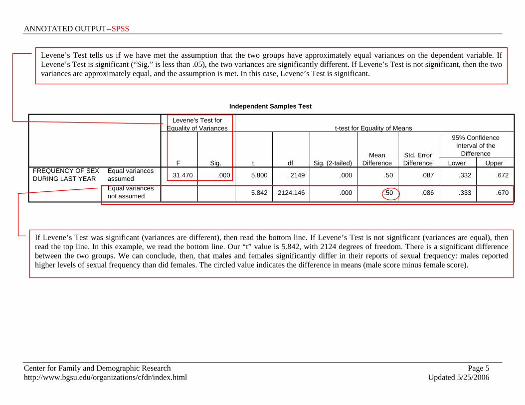
Crosstab (with Chi-Square) A crosstabulation displays the number of cases in each category defined by two or more grouping variables. CROSSTABS /TABLES=happy BY freqdum /FORMAT= AVALUE TABLES /STATISTIC=CHISQ /CELLS= COUNT EXPECTED /COUNT ROUND CELL .

Case Processing Summary

1060 38.3% 1705 61.7% 2765 100.0%GENERAL HAPPINESS *SEXFREQ (Monthly+ =1)

N Percent N Percent N PercentValid Missing Total

Cases

GENERAL HAPPINESS * SEXFREQ (Monthly+ =1) Crosstabulation

103 207 310132.2 177.8 310.0

286 333 619264.0 355.0 619.0

63 68 13155.9 75.1 131.0452 608 1060

452.0 608.0 1060.0

CountExpected CountCountExpected CountCountExpected CountCountExpected Count

VERY HAPPY (1)

PRETTY HAPPY (2)

NOT TOO HAPPY (3)

GENERALHAPPINESS

Total

Less thanof equal to1/month

More than1/month

SEXFREQ (Monthly+ =1)

Total

For example, we see that there are 207 cases reporting “very happy” for general happiness and “more than once per month” for frequency of sex.



Chi-Square Tests

16.039a 2 .00016.297 2 .000

13.123 1 .000

1060

Pearson Chi-SquareLikelihood RatioLinear-by-LinearAssociationN of Valid Cases

Value dfAsymp. Sig.

(2-sided)

0 cells (.0%) have expected count less than 5. Theminimum expected count is 55.86.

a.

The Chi-Square measure tests the hypothesis that the row and column variables in a crosstabulation are independent of one another. While the Chi-Square measure may indicate that there is a relationship between two variables, they do not indicate the strength or direction of the relationship.

The cell size note checks for a validation of one of the Chi Square assumptions: If one or more of the cells has less than 5, then use Fisher’s test.



Chi-Square The Chi-Square Goodness of Fit Test determines if the observed frequencies are different from what we would expect to find (we expect equal numbers in each group within a variable). Use a Chi-Square Test when you want to know if there is a significant relationship between two categorical variables. In this example, we use “frequency of sex” and “happiness.” Null Hypothesis: There are approximately equal numbers of cases in each group. Alternate Hypothesis: There are not equal numbers of cases in each group. NPAR TEST /CHISQUARE=happy /EXPECTED=EQUAL /MISSING ANALYSIS.

GENERAL HAPPINESS

415 456.3 -41.3784 456.3 327.7170 456.3 -286.3

1369

VERY HAPPYPRETTY HAPPYNOT TOO HAPPYTotal

Observed N Expected N Residual

Test Statistics

418.6872

.000

Chi-Squarea

dfAsymp. Sig.

GENERALHAPPINESS

0 cells (.0%) have expected frequencies less than5. The minimum expected cell frequency is 456.3.

a.

We have a Chi-Square value of 418.7, which is large. Our significance level is .000. We can conclude that there are not equal numbers of cases in each happiness category.

The cell size note checks for a validation of one of the Chi Square assumptions: If one or more of the cells has less than 5, then use Fisher’s test.



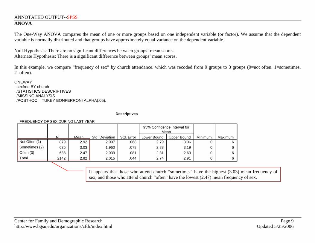
ANOVA The One-Way ANOVA compares the mean of one or more groups based on one independent variable (or factor). We assume that the dependent variable is normally distributed and that groups have approximately equal variance on the dependent variable. Null Hypothesis: There are no significant differences between groups’ mean scores. Alternate Hypothesis: There is a significant difference between groups’ mean scores. In this example, we compare “frequency of sex” by church attendance, which was recoded from 9 groups to 3 groups (0=not often, 1=sometimes, 2=often). ONEWAY sexfreq BY church /STATISTICS DESCRIPTIVES /MISSING ANALYSIS /POSTHOC = TUKEY BONFERRONI ALPHA(.05).

Descriptives

FREQUENCY OF SEX DURING LAST YEAR

879 2.92 2.007 .068 2.79 3.06 0 6625 3.03 1.960 .078 2.88 3.19 0 6638 2.47 2.039 .081 2.31 2.63 0 6

2142 2.82 2.015 .044 2.74 2.91 0 6

Not Often (1)Sometimes (2)Often (3)Total

N Mean Std. Deviation Std. Error Lower Bound Upper Bound

95% Confidence Interval forMean

Minimum Maximum

It appears that those who attend church “sometimes” have the highest (3.03) mean frequency of sex, and those who attend church “often” have the lowest (2.47) mean frequency of sex.



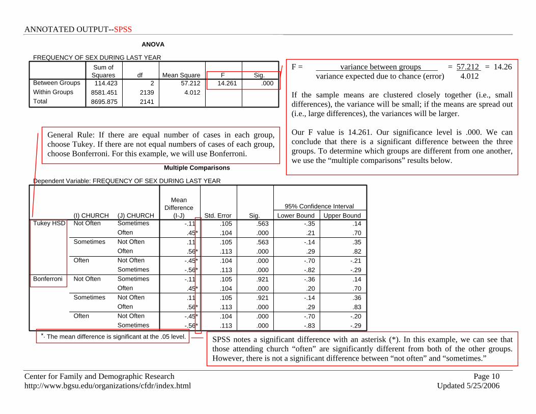
ANOVA

FREQUENCY OF SEX DURING LAST YEAR

114.423 2 57.212 14.261 .0008581.451 2139 4.0128695.875 2141

Between GroupsWithin GroupsTotal

Sum ofSquares df Mean Square F Sig.

Multiple Comparisons

Dependent Variable: FREQUENCY OF SEX DURING LAST YEAR

-.11 .105 .563 -.35 .14.45* .104 .000 .21 .70.11 .105 .563 -.14 .35.56* .113 .000 .29 .82

-.45* .104 .000 -.70 -.21-.56* .113 .000 -.82 -.29-.11 .105 .921 -.36 .14.45* .104 .000 .20 .70.11 .105 .921 -.14 .36.56* .113 .000 .29 .83

-.45* .104 .000 -.70 -.20-.56* .113 .000 -.83 -.29

(J) CHURCHSometimesOftenNot OftenOftenNot OftenSometimesSometimesOftenNot OftenOftenNot OftenSometimes

(I) CHURCHNot Often

Sometimes

Often

Not Often

Sometimes

Often

Tukey HSD

Bonferroni

MeanDifference

(I-J) Std. Error Sig. Lower Bound Upper Bound95% Confidence Interval

The mean difference is significant at the .05 level.*.

F = variance between groups = 57.212 = 14.26 variance expected due to chance (error) 4.012

If the sample means are clustered closely together (i.e., small differences), the variance will be small; if the means are spread out (i.e., large differences), the variances will be larger. Our F value is 14.261. Our significance level is .000. We can conclude that there is a significant difference between the three groups. To determine which groups are different from one another, we use the “multiple comparisons” results below.

General Rule: If there are equal number of cases in each group, choose Tukey. If there are not equal numbers of cases of each group, choose Bonferroni. For this example, we will use Bonferroni.

SPSS notes a significant difference with an asterisk (*). In this example, we can see that those attending church “often” are significantly different from both of the other groups. However, there is not a significant difference between “not often” and “sometimes.”



Simple Linear (OLS) Regression Regression is a method for studying the relationship of a dependent variable and one or more independent variables. Simple Linear Regression tells you the amount of variance accounted for by one variable in predicting another variable. In this example, we are interested in predicting the frequency of sex among a national sample of adults. The dependent variable is frequency of sex. The independent variables are: age, race, general happiness, church attendance, and marital status. REGRESSION /MISSING LISTWISE /STATISTICS COEFF OUTS R ANOVA /CRITERIA=PIN(.05) POUT(.10) /NOORIGIN /DEPENDENT sexfreq /METHOD=ENTER age Married White happy attend .

Variables Entered/Removedb

CHURCHATTENDANCE,RACE(White =1),GENERALHAPPINESS, AGE,MARITAL(Married=1)

a

. Enter

Model1

VariablesEntered

VariablesRemoved Method

All requested variables entered.a.

Dependent Variable: FREQUENCY OFSEX DURING LAST YEAR

b.



Model Summary

.572a .327 .323 1.651Model1

RR Square

-a-

AdjustedR Square

-b-

Std. Error ofthe Estimate

-c-

Predictors: (Constant), CHURCH ATTENDANCE,RACE (White =1), GENERAL HAPPINESS, AGE,MARITAL (Married =1)

a.

a. “R Square” = tells us how much of the variance of the dependent variable can be explained by the independent variable(s). Basically, it compares the model with the independent variables to a model without the independent variables. In this case, 33% of the variance is explained by differences in all included variables. b. “Adjusted R Square” = As predictors are added to the model, each predictor will explain some of the variance in the dependent variable simply due to chance. The Adjusted R Square attempts to produce a more honest value to estimate R Square for the population. In this example, the difference between R Square and Adjusted R Square is minimal. c. “Std. Error” = The standard error of the estimate (aka, the root mean square error), is the standard deviation of the error term, and is the square root of the Mean Square Residual (or Error).



ANOVAb

1382.662 5 276.532 101.490 .000a

2850.064 1046 2.7254232.726 1051

Regression -d-Residual -e-Total

Model1

Sum ofSquares

-f- df Mean Square F -g- Sig.

Predictors: (Constant), CHURCH ATTENDANCE, RACE (White =1), GENERALHAPPINESS, AGE, MARITAL (Married =1)

a.

Dependent Variable: FREQUENCY OF SEX DURING LAST YEARb.

d. The output for “Regression” displays information about the variation accounted for by the model. e. The output for “Residual” displays information about the variation that is not accounted for by your model. And the output for “Total” is the sum of the information for Regression and Residual. f. A model with a large regression sum of squares in comparison to the residual sum of squares indicates that the model accounts for most of variation in the dependent variable. Very high residual sum of squares indicate that the model fails to explain a lot of the variation in the dependent variable, and you may want to look for additional factors that help account for a higher proportion of the variation in the dependent variable. In this example, we see that 32.7% of the total sum of squares is made up from the regression sum of squares. You may notice that the R2 for this model is also .327 (this is not a coincidence!). g. If the significance value of the F statistic is small (smaller than say 0.05) then the independent variables do a good job explaining the variation in the dependent variable. If the significance value of F is larger than say 0.05 then the independent variables do not explain the variation in the dependent variable. For this example the model does a good job explaining the variation in the dependent variable.



Coefficientsa

5.553 .250 22.191 .000-.055 .003 -.475 -18.255 .0001.372 .107 .339 12.810 .000-.215 .125 -.045 -1.719 .086-.262 .085 -.081 -3.094 .002-.067 .020 -.089 -3.436 .001

(Constant) -h-AGEMARITAL (Married =1)RACE (White =1)GENERAL HAPPINESSCHURCH ATTENDANCE

Model1

B Std. Error

UnstandardizedCoefficients -i-

Beta

StandardizedCoefficients -j-

t -k- Sig. -l-

Dependent Variable: FREQUENCY OF SEX DURING LAST YEARa.

h. “Constant” represents the Y-intercept, the height of the regression line when it crosses the Y axis. In this example, it is the predicted value of the dependent variable, “frequency of sex,” when all other values are zero (0). In this example, the value is 5.553. i. These are the values for the regression equation for predicting the dependent variable from the independent variable(s). These are unstandardized (B) coefficients because they are measured in natural units, and therefore cannot be compared to one another to determine which is more influential. j. The standardized coefficients or betas are an attempt to make the regression coefficients more comparable. Here we can see that the Beta for age has the largest absolute value (-.475), which can be interpreted as having the greatest impact on frequency of sex compared to the other variables in the model. The race variable has the smallest absolute value (-.045) and can be interpreted as having the smallest impact of the dependent variable. k. The t statistics can help you determine the relative importance of each variable in the model. The t-statistic is calculated by divided the variable’s unstandardized coefficient by its standard error. As a guide regarding useful predictors, look for t values well below -1.96 or above +1.96. As you can see, the race variable is the only t-value not within this range (note also that this is the only variable that is not significant). l. The significance column indicates whether or not a variable is a significant predictor of the dependent variable. The p-value (significance) is the probability that your sample could have been drawn from the population(s) being tested (or that a more improbable sample could be drawn) given the assumption that the null hypothesis is true. A p-value of .05, for example, indicates that you would have only a 5% chance of drawing the sample being tested if the null hypothesis was actually true. As sociologists, we typically look for p-values below .05. For example, in this model the race variable is not significant (p = .086), while the other variables are significant.



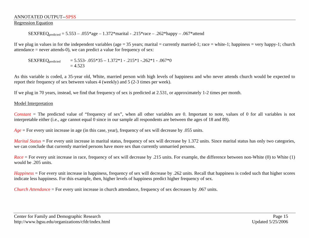
Regression Equation

SEXFREQpredicted = 5.553 – .055*age – 1.372*marital - .215*race – .262*happy – .067*attend If we plug in values in for the independent variables (age = 35 years; marital = currently married-1; race = white-1; happiness = very happy-1; church attendance = never attends-0), we can predict a value for frequency of sex:

SEXFREQpredicted = 5.553- .055*35 – 1.372*1 - .215*1 -.262*1 - .067*0 = 4.523

As this variable is coded, a 35-year old, White, married person with high levels of happiness and who never attends church would be expected to report their frequency of sex between values 4 (weekly) and 5 (2-3 times per week). If we plug in 70 years, instead, we find that frequency of sex is predicted at 2.531, or approximately 1-2 times per month. Model Interpretation Constant = The predicted value of “frequency of sex”, when all other variables are 0. Important to note, values of 0 for all variables is not interpretable either (i.e., age cannot equal 0 since in our sample all respondents are between the ages of 18 and 89). Age = For every unit increase in age (in this case, year), frequency of sex will decrease by .055 units. Marital Status = For every unit increase in marital status, frequency of sex will decrease by 1.372 units. Since marital status has only two categories, we can conclude that currently married persons have more sex than currently unmarried persons. Race = For every unit increase in race, frequency of sex will decrease by .215 units. For example, the difference between non-White (0) to White (1) would be .205 units. Happiness = For every unit increase in happiness, frequency of sex will decrease by .262 units. Recall that happiness is coded such that higher scores indicate less happiness. For this example, then, higher levels of happiness predict higher frequency of sex. Church Attendance = For every unit increase in church attendance, frequency of sex decreases by .067 units.



Simple Linear Regression (with nonlinear variables) It is known that some variables are often non-linear, or curvilinear. Such variables may be age or income. In this example, we include the original age variable and an age squared variable. REGRESSION /MISSING LISTWISE /STATISTICS COEFF OUTS R ANOVA /CRITERIA=PIN(.05) POUT(.10) /NOORIGIN /DEPENDENT sexfreq /METHOD=ENTER age Married White happy attend agesquare .

Coefficientsa

4.838 .427 11.329 .000-.020 .017 -.175 -1.190 .2341.314 .111 .325 11.883 .000-.218 .125 -.046 -1.745 .081-.271 .085 -.084 -3.207 .001-.067 .020 -.089 -3.423 .001.000 .000 -.303 -2.065 .039

(Constant)AGEMARITAL (Married =1)RACE (White =1)GENERAL HAPPINESSCHURCH ATTENDANCEAGE-SQUARED

Model1

B Std. Error

UnstandardizedCoefficients

Beta

StandardizedCoefficients

t Sig.


The age squared variable is significant, indicating that age is non-linear.



Simple Linear Regression (with interaction term) In a linear model, the effect of each independent variable is always the same. However, it could be that the effect of one variable depends on another. In this example, we might expect that the effect of marital status is dependent on gender. In the following example, we include an interaction term, male*married. To test for two-way interactions (often thought of as a relationship between an independent variable (IV) and dependent variable (DV), moderated by a third variable), first run a regression analysis, including both independent variables (IV and moderator) and their interaction (product) term. It is highly recommended that the independent variable and moderator are standardized before calculation of the product term, although this is not essential. For this example, two dummy variables were created, for ease of interpretation. Gender was coded such that 1=Male and 0=Female. Marital status was coded such that 1=Currently married and 0=Not currently married. The interaction term is a cross-product of these two dummy variables. Regression Model (without interactions) REGRESSION /MISSING LISTWISE /STATISTICS COEFF OUTS R ANOVA /CRITERIA=PIN(.05) POUT(.10) /NOORIGIN /DEPENDENT sexfreq /METHOD=ENTER age White happy attend Male Married .

Coefficientsa

5.295 .258 20.503 .000-.055 .003 -.469 -18.089 .000-.231 .125 -.048 -1.852 .064-.242 .084 -.075 -2.873 .004-.056 .020 -.074 -2.850 .004.385 .104 .096 3.709 .000

1.318 .107 .326 12.262 .000

(Constant)AGERACE (White =1)GENERAL HAPPINESSCHURCH ATTENDANCEGENDER (Male =1)MARITAL (Married =1)

Model1

B Std. Error


Beta


t Sig.




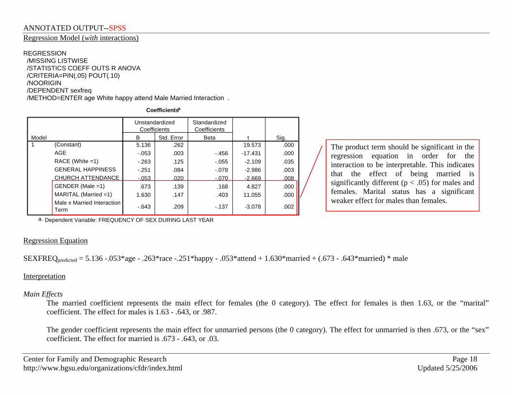
Regression Model (with interactions) REGRESSION /MISSING LISTWISE /STATISTICS COEFF OUTS R ANOVA /CRITERIA=PIN(.05) POUT(.10) /NOORIGIN /DEPENDENT sexfreq /METHOD=ENTER age White happy attend Male Married Interaction .

Coefficientsa

5.136 .262 19.573 .000-.053 .003 -.456 -17.431 .000-.263 .125 -.055 -2.109 .035-.251 .084 -.078 -2.986 .003-.053 .020 -.070 -2.669 .008.673 .139 .168 4.827 .000

1.630 .147 .403 11.055 .000

-.643 .209 -.137 -3.078 .002

(Constant)AGERACE (White =1)GENERAL HAPPINESSCHURCH ATTENDANCEGENDER (Male =1)MARITAL (Married =1)Male x Married InteractionTerm

Model1

B Std. Error


Beta


t Sig.


Regression Equation SEXFREQpredicted = 5.136 -.053*age - .263*race -.251*happy - .053*attend + 1.630*married + (.673 - .643*married) * male Interpretation Main Effects

The married coefficient represents the main effect for females (the 0 category). The effect for females is then 1.63, or the “marital” coefficient. The effect for males is 1.63 - .643, or .987. The gender coefficient represents the main effect for unmarried persons (the 0 category). The effect for unmarried is then .673, or the “sex” coefficient. The effect for married is .673 - .643, or .03.

The product term should be significant in the regression equation in order for the interaction to be interpretable. This indicates that the effect of being married is significantly different (p < .05) for males and females. Marital status has a significant weaker effect for males than females.



Interaction Effects For a simple interpretation of the interaction term, plug values into the regression equation above.

Married Men = SEXFREQpredicted = 5.136 -.053*35 - .263*1 -.251*1 - .053*0 + 1.630*1 + (.673 - . 643*1) * 1 = 5.455 Married Women = SEXFREQpredicted = 5.136 -.053*35 - .263*1 -.251*1 - .053*0 + 1.630*1 + (.673 - . 643*1) * 0 = 5.425 Unmarried Men = SEXFREQpredicted = 5.136 -.053*35 - .263*1 -.251*1 - .053*0 + 1.630*0 + (.673 - . 643*0) * 1 = 3.825 Unmarried Women = SEXFREQpredicted = 5.136 -.053*35 - .263*1 -.251*1 - .053*0 + 1.630*0 + (.673 - . 643*0) * 0 = 3.795

In this example (age = 35 years; race = white-1; happiness = very happy-1; church attendance = never attends-0), we can see that (1) for both married and unmarried persons, males are reporting higher frequency of sex than females, and (2) married persons report higher frequency of sex than unmarried persons. The interaction tells us that the gender difference is greater for married persons than for unmarried persons.



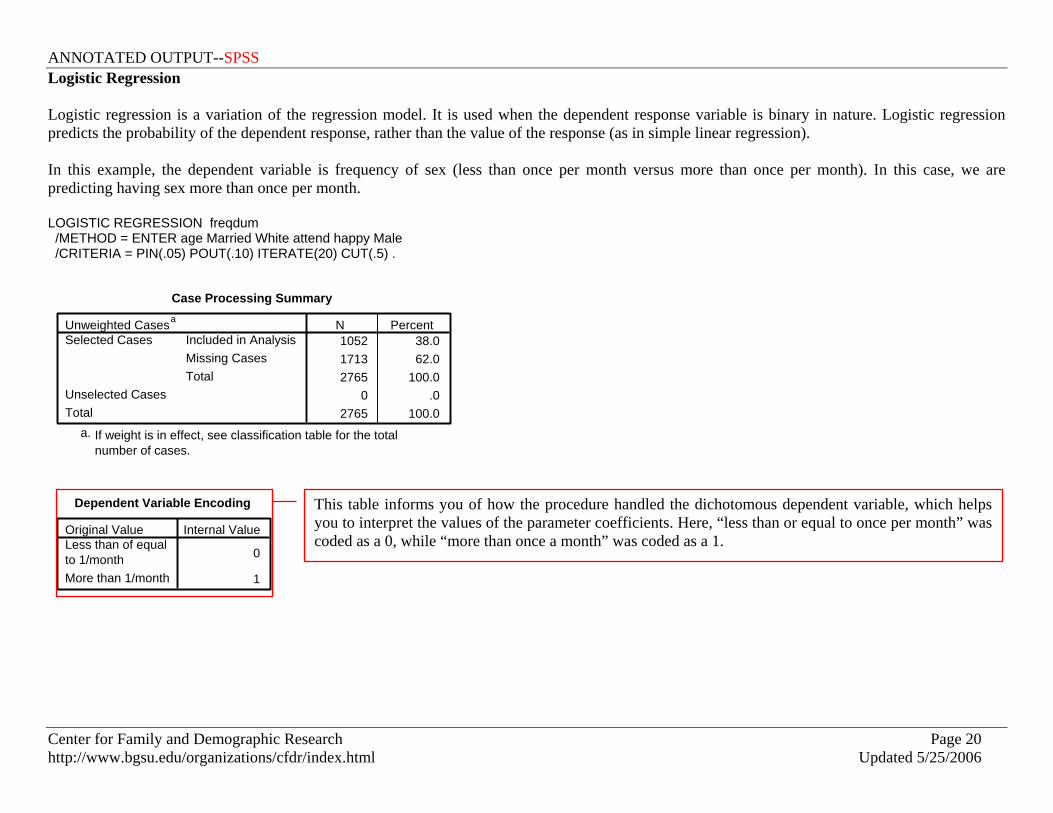
Logistic Regression Logistic regression is a variation of the regression model. It is used when the dependent response variable is binary in nature. Logistic regression predicts the probability of the dependent response, rather than the value of the response (as in simple linear regression). In this example, the dependent variable is frequency of sex (less than once per month versus more than once per month). In this case, we are predicting having sex more than once per month. LOGISTIC REGRESSION freqdum /METHOD = ENTER age Married White attend happy Male /CRITERIA = PIN(.05) POUT(.10) ITERATE(20) CUT(.5) .

Case Processing Summary

1052 38.01713 62.02765 100.0

0 .02765 100.0

Unweighted Casesa

Included in AnalysisMissing CasesTotal

Selected Cases

Unselected CasesTotal

N Percent

If weight is in effect, see classification table for the totalnumber of cases.

a.

Dependent Variable Encoding

0

1

Original ValueLess than of equalto 1/monthMore than 1/month

Internal Value

This table informs you of how the procedure handled the dichotomous dependent variable, which helps you to interpret the values of the parameter coefficients. Here, “less than or equal to once per month” was coded as a 0, while “more than once a month” was coded as a 1.



Block 1: Method = Enter

Omnibus Tests of Model Coefficients

311.100 6 .000311.100 6 .000311.100 6 .000

StepBlockModel

Step 1Chi-square df Sig.

Model Summary

1125.821a .256 .344Step1

-2 Loglikelihood

Cox & SnellR Square

NagelkerkeR Square

Estimation terminated at iteration number 5 becauseparameter estimates changed by less than .001.

a.

Classification Tablea

262 189 58.1

109 492 81.971.7

ObservedLess than of equalto 1/monthMore than 1/month

SEXFREQ(Monthly+ =1)

Overall Percentage

Step 1

Less thanof equal to1/month

More than1/month

SEXFREQ (Monthly+ =1)

PercentageCorrect

Predicted

The cut value is .500a.

The omnibus tests are measures of how well the model performs.

The chi-square statistic is the change in the -2 log-likelihood from the previous step, block, or model. If the step was to remove a variable, the exclusion makes sense if the significance of the change is large (i.e., greater than 0.10). If the step was to add a variable, the inclusion makes sense if the significance of the change is small (i.e., less than 0.05). In this example, the change is from Block 0, where no variables are entered.

The R-Square statistic cannot be exactly computed for logistic regression models, so these approximations are computed instead. Larger pseudo r-square statistics indicate that more of the variation is explained by the model, to a maximum of 1.

The classification table helps you to assess the performance of your model by crosstabulating the observed response categories with the predicted response categories. For each case, the predicted response is the category treated as 1, if that category's predicted probability is greater than the user-specified cutoff. Cells on the diagonal are correct predictions.



Variables in the Equation

-.061 .005 145.748 1 .000 .9411.698 .167 103.127 1 .000 5.465-.149 .178 .699 1 .403 .862-.059 .029 4.315 1 .038 .942-.318 .123 6.723 1 .010 .727.444 .148 8.951 1 .003 1.558

3.047 .382 63.773 1 .000 21.054

ageMarriedWhiteattendhappyMaleConstant

Step1

a

B -b- S.E. -b- Wald -c- df Sig. Exp(B) -d-

Variable(s) entered on step 1: age, Married, White, attend, happy, Male.a.

b. B is the estimated coefficient, with standard error, S.E. c. The ratio of B to S.E., squared, equals the Wald statistic. If the Wald statistic is significant (i.e., less than 0.05) then the parameter is useful to the model. d. “Exp(B),” or the odds ratio, is the predicted change in odds for a unit increase in the predictor. The “exp” refers to the exponential value of B. When Exp(B) is less than 1, increasing values of the variable correspond to decreasing odds of the event's occurrence. When Exp(B) is greater than 1, increasing values of the variable correspond to increasing odds of the event's occurrence. If you subtract 1 from the odds ratio and multiply by 100, you get the percent change in odds of the dependent variable having a value of 1. For example, for age:

= 1 - (.941) = .051 = .051 * 100 = 5.1%

The odds ratio for age indicates that every unit increase in age is associated with a 5.1% decrease in the odds of having sex more than once a month. Regression Equation FREQDUMPREDICTED = 3.047 - .061*age – 1.698*married - .149*white – .059*attend - .318*happiness + .444*male If we plug in values in for the independent variables (age = 35 years; married = currently married-1; race = white-1; happiness = very happy-1; church attendance = never attends-0; gender = male-1), we can predict a value for frequency of sex:

FREQDUMpredicted = 3.047 - .061*35 – 1.698*1 - .149*1 – .059*0 - .318*1 + .444*1 = 2.587



As this variable is coded, a 35-year old, White, married person with high levels of happiness and who never attends church would be expected to report their frequency of sex between values 4 (weekly) and 5 (2-3 times per week). If we plug in 70 years, instead, we find that frequency of sex is predicted at 2.455, or approximately 1-2 times per month. Interpretation Recall: When Exp(B) is less than 1, increasing values of the variable correspond to decreasing odds of the event's occurrence. When Exp(B) is greater than 1, increasing values of the variable correspond to increasing odds of the event's occurrence. Constant = Not interpretable in logistic regression. Age = Increasing values of age correspond with decreasing odds of having sex more than once a month. Marital = Married persons have a decreased odds of having sex more than once a month. Race = White persons have a decreased odds of having sex more than once a month. Notice that this variable, however, is not significant. Church Attendance = Increasing values of church attendance correspond with decreasing odds of having sex more than once a month. Happiness = Increasing values of general happiness correspond with decreasing odds of having sex more than once a month. Recall that happiness is coded such that higher values indicate less happiness.



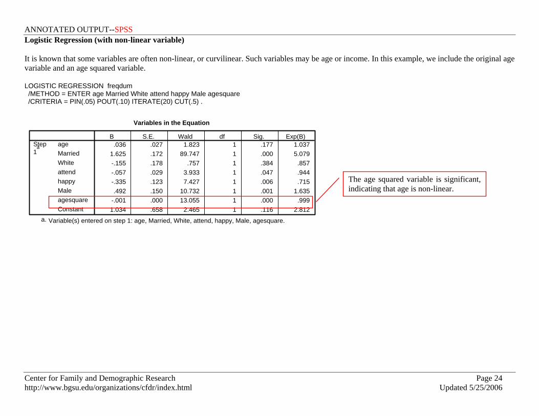
Logistic Regression (with non-linear variable) It is known that some variables are often non-linear, or curvilinear. Such variables may be age or income. In this example, we include the original age variable and an age squared variable. LOGISTIC REGRESSION freqdum /METHOD = ENTER age Married White attend happy Male agesquare /CRITERIA = PIN(.05) POUT(.10) ITERATE(20) CUT(.5) .


.036 .027 1.823 1 .177 1.0371.625 .172 89.747 1 .000 5.079-.155 .178 .757 1 .384 .857-.057 .029 3.933 1 .047 .944-.335 .123 7.427 1 .006 .715.492 .150 10.732 1 .001 1.635

-.001 .000 13.055 1 .000 .9991.034 .658 2.465 1 .116 2.812

ageMarriedWhiteattendhappyMaleagesquareConstant

Step1

a

B S.E. Wald df Sig. Exp(B)

Variable(s) entered on step 1: age, Married, White, attend, happy, Male, agesquare.a.

The age squared variable is significant, indicating that age is non-linear.



Logistic Regression (with interaction term) To test for two-way interactions (often thought of as a relationship between an independent variable (IV) and dependent variable (DV), moderated by a third variable), first run a regression analysis, including both independent variables (IV and moderator) and their interaction (product) term. It is highly recommended that the independent variable and moderator are standardized before calculation of the product term, although this is not essential. For this example, two dummy variables were created, for ease of interpretation. Sex was recoded such that 1=Male and 0=Female. Marital status was recoded such that 1=Currently married and 0=Not currently married. The interaction term is a product of these two dummy variables. Regression Model (without interactions) LOGISTIC REGRESSION freqdum /METHOD = ENTER age White attend happy Male Married /CRITERIA = PIN(.05) POUT(.10) ITERATE(20) CUT(.5) .


-.061 .005 145.748 1 .000 .941-.149 .178 .699 1 .403 .862-.059 .029 4.315 1 .038 .942-.318 .123 6.723 1 .010 .727.444 .148 8.951 1 .003 1.558

1.698 .167 103.127 1 .000 5.4653.047 .382 63.773 1 .000 21.054

ageWhiteattendhappyMaleMarriedConstant

Step1

a


Variable(s) entered on step 1: age, White, attend, happy, Male, Married.a.



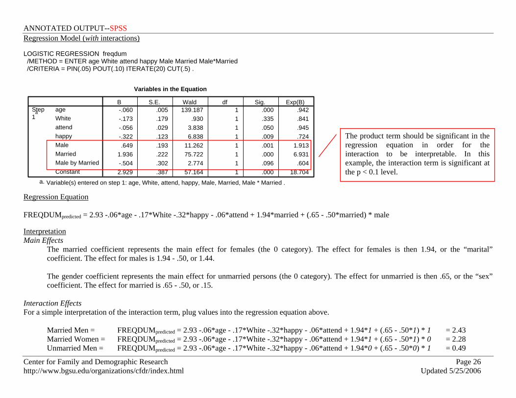
Regression Model (with interactions) LOGISTIC REGRESSION freqdum /METHOD = ENTER age White attend happy Male Married Male*Married /CRITERIA = PIN(.05) POUT(.10) ITERATE(20) CUT(.5) .


-.060 .005 139.187 1 .000 .942-.173 .179 .930 1 .335 .841-.056 .029 3.838 1 .050 .945-.322 .123 6.838 1 .009 .724.649 .193 11.262 1 .001 1.913

1.936 .222 75.722 1 .000 6.931-.504 .302 2.774 1 .096 .6042.929 .387 57.164 1 .000 18.704

ageWhiteattendhappyMaleMarriedMale by MarriedConstant

Step1

a


Variable(s) entered on step 1: age, White, attend, happy, Male, Married, Male * Married .a.

Regression Equation FREQDUMpredicted = 2.93 -.06*age - .17*White -.32*happy - .06*attend + 1.94*married + (.65 - .50*married) * male Interpretation Main Effects

The married coefficient represents the main effect for females (the 0 category). The effect for females is then 1.94, or the “marital” coefficient. The effect for males is 1.94 - .50, or 1.44. The gender coefficient represents the main effect for unmarried persons (the 0 category). The effect for unmarried is then .65, or the “sex” coefficient. The effect for married is .65 - .50, or .15.

Interaction Effects For a simple interpretation of the interaction term, plug values into the regression equation above.

Married Men = FREQDUMpredicted = 2.93 -.06*age - .17*White -.32*happy - .06*attend + 1.94*1 + (.65 - .50*1) * 1 = 2.43 Married Women = FREQDUMpredicted = 2.93 -.06*age - .17*White -.32*happy - .06*attend + 1.94*1 + (.65 - .50*1) * 0 = 2.28 Unmarried Men = FREQDUMpredicted = 2.93 -.06*age - .17*White -.32*happy - .06*attend + 1.94*0 + (.65 - .50*0) * 1 = 0.49

The product term should be significant in the regression equation in order for the interaction to be interpretable. In this example, the interaction term is significant at the p < 0.1 level.



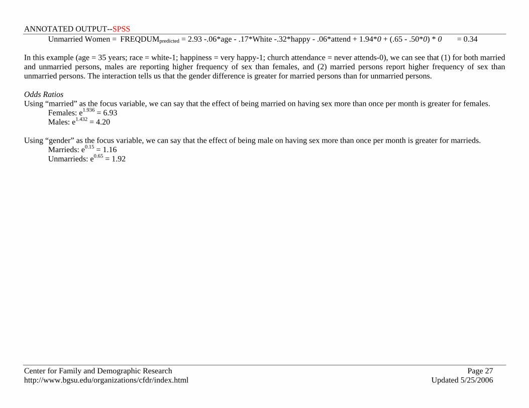
Unmarried Women = FREQDUMpredicted = 2.93 -.06*age - .17*White -.32*happy - .06*attend + 1.94*0 + (.65 - .50*0) * 0 = 0.34

In this example (age = 35 years; race = white-1; happiness = very happy-1; church attendance = never attends-0), we can see that (1) for both married and unmarried persons, males are reporting higher frequency of sex than females, and (2) married persons report higher frequency of sex than unmarried persons. The interaction tells us that the gender difference is greater for married persons than for unmarried persons. Odds Ratios Using “married” as the focus variable, we can say that the effect of being married on having sex more than once per month is greater for females.

Females: e1.936 = 6.93 Males: e1.432 = 4.20

Using “gender” as the focus variable, we can say that the effect of being male on having sex more than once per month is greater for marrieds. Marrieds: e0.15 = 1.16 Unmarrieds: e0.65 = 1.92

ANNOTATED OUTPUT--SPSS Descriptive Statistics · 2013-12-20 · SPSS considers these values...

Documents

Transcript of ANNOTATED OUTPUT--SPSS Descriptive Statistics · 2013-12-20 · SPSS considers these values...